Embed Size (px)
Citation preview

Wireless CommunicationElec 534
Set IVOctober 23, 2007
Behnaam Aazhang

Reading for Set 4
• Tse and Viswanath– Chapters 7,8– Appendices B.6,B.7
• Goldsmith– Chapters 10

Outline
• Channel model• Basics of multiuser systems• Basics of information theory• Information capacity of single antenna single
user channels– AWGN channels– Ergodic fast fading channels– Slow fading channels
• Outage probability• Outage capacity

Outline
• Communication with additional dimensions– Multiple input multiple output (MIMO)
• Achievable rates• Diversity multiplexing tradeoff• Transmission techniques
– User cooperation• Achievable rates• Transmission techniques
Dimension
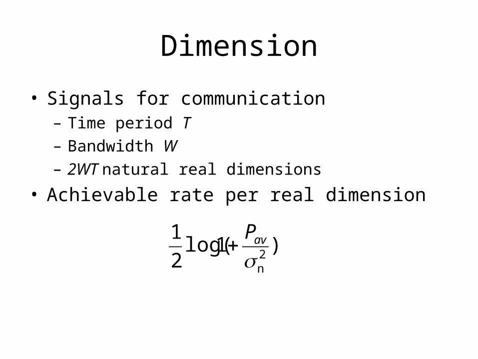
• Signals for communication– Time period T– Bandwidth W– 2WT natural real dimensions
• Achievable rate per real dimension
)1log(2
12navP

Communication with Additional Dimensions: An Example
• Adding the Q channel– BPSK to QPSK
• Modulated both real and
imaginary signal dimensions• Double the data rate• Same bit error probability
)2
(0N
EQP b
e

Communication with Additional Dimensions
• Larger signal dimension--larger capacity– Linear relation
• Other degrees of freedom (beyond signaling)– Spatial– Cooperation
• Metric to measure impact on– Rate (multiplexing)– Reliability (diversity)
• Same metric for– Feedback– Opportunistic access
Multiplexing Gain
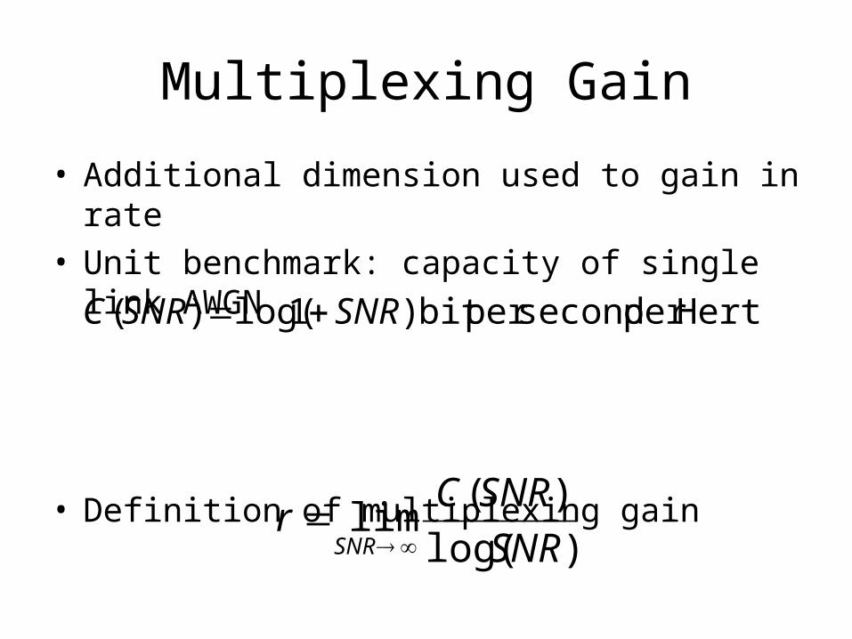
• Additional dimension used to gain in rate• Unit benchmark: capacity of single link AWGN
• Definition of multiplexing gain
Hertzper secondper bit )1log()( SNRSNRC
)log(
)(lim
SNR
SNRCr
SNR
Diversity Gain
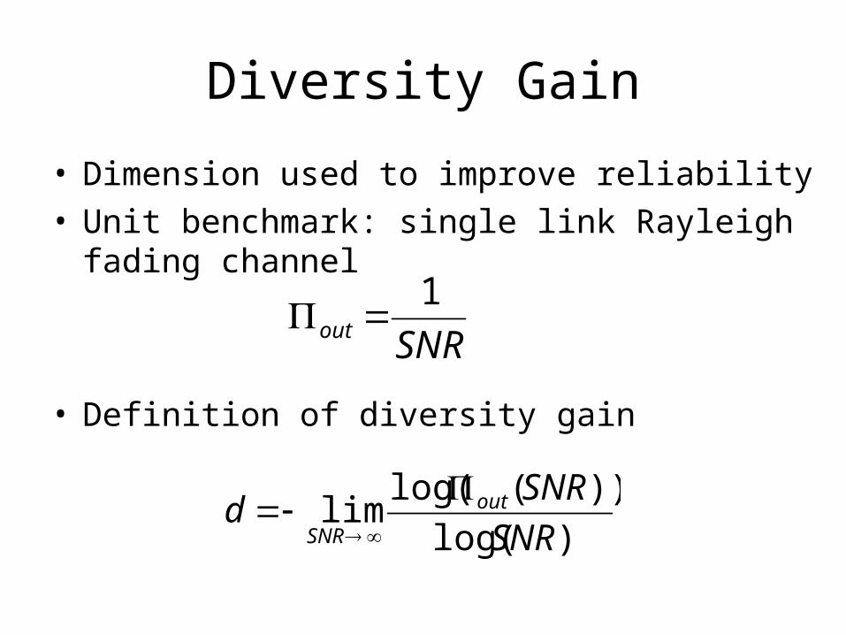
• Dimension used to improve reliability• Unit benchmark: single link Rayleigh fading
channel
• Definition of diversity gain
SNRout
1
)log(
))(log(lim
SNR
SNRd out
SNR

Multiple Antennas
• Improve fading and increase data rate• Additional degrees of freedom
– virtual/physical channels– tradeoff between diversity and multiplexing
Transmitter Receiver

Multiple Antennas
• The model
where Tc is the coherence time
cRcTTRcR TMTMMMTM nbHr
Transmitter Receiver
Basic Assumption
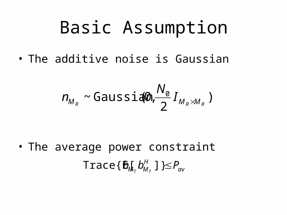
• The additive noise is Gaussian
• The average power constraint
)2
,0(Gaussian~ 0RRR MMM I
Nn
avHMM Pbb
TT]}Trace{E[

Matrices
• A channel matrix
• Trace of a square matrix
**
*1
*11
1
111
1
,
RMTMRM
T
RT
RTT
R
TR
hh
hh
H
hh
hh
HM
HMM
MMM
M
MM
M
iiiMM hH
1
]Trace[
Matrices
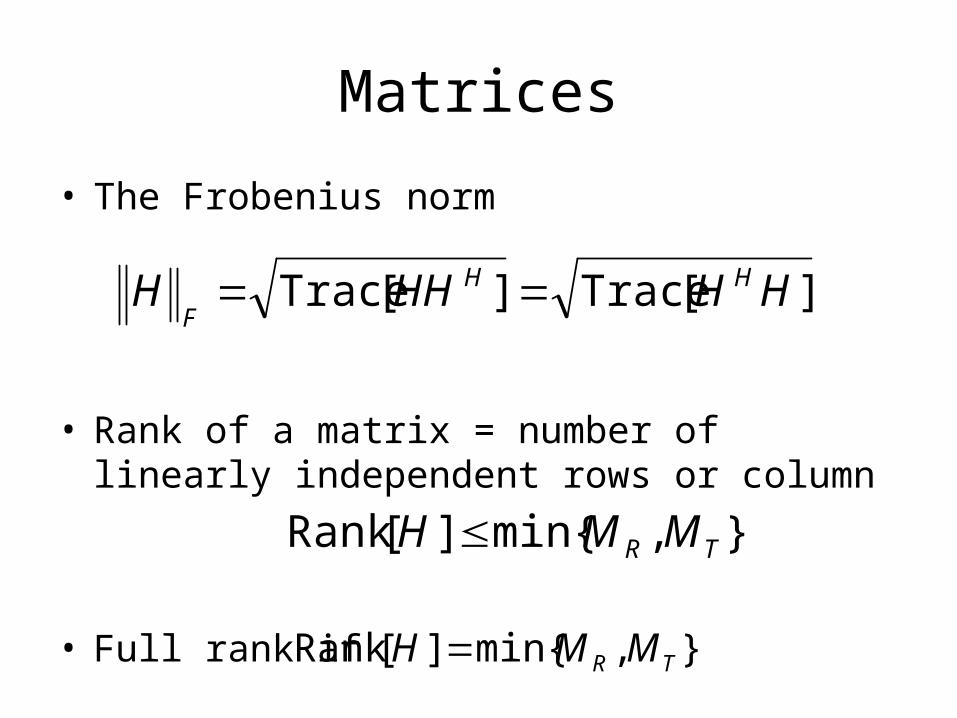
• The Frobenius norm
• Rank of a matrix = number of linearly independent rows or column
• Full rank if
][Trace][Trace HHHHH HH
F
},min{][Rank TR MMH
},min{][Rank TR MMH

Matrices
• A square matrix is invertible if there is a matrix
• The determinant—a measure of how noninvertible a matrix is!
• A square invertible matrix U is unitary if
IAA 1
IUU H

Matrices• Vector X is rotated and scaled by a matrix A
• A vector X is called the eigenvector of the matrix and lambda is the eigenvalue if
• Then
with unitary and diagonal matrices
Axy
xAx
HUUA

Matrices• The columns of unitary matrix U are
eigenvectors of A• Determinant is the product of all eigenvalues • The diagonal matrix
N
0
01

Matrices
• If H is a non square matrix then
• Unitary U with columns as the left singular vectors and unitary V matrix with columns as the right singular vectors
• The diagonal matrix
HMMMMMM TTTMRMRRTR
VUH
00
00
or
00
0
0
1
1
R
TTR
M
MMM

Matrices
• The singular values of H are square root of eigenvalues of square H
)(eigenvalue
)singular(
iH
MMMM
MMi
RTTR
TR
HH
H

MIMO Channels
• There are channels– Independent if
• Sufficient separation compared to carrier wavelength• Rich scattering
– At transmitter– At receiver
• The number of singular vectors of the channel
• The singular vectors are the additional (spatial) degrees of freedom
RT MM
},min{ RT MM

Channel State Information
• More critical than SISO– CSI at transmitter and received– CSI at receiver– No CSI
• Forward training
• Feedback or reverse training
Fixed MIMO Channel
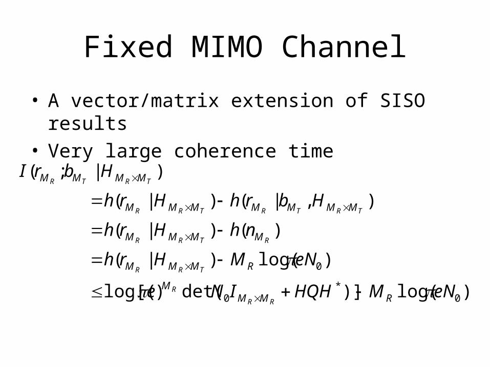
• A vector/matrix extension of SISO results• Very large coherence time
)log()]det()log[(
)log()|(
)()|(
),|()|(
)|;(
0*
0
0
eNMHQHINe
eNMHrh
nhHrh
HbrhHrh
HbrI
RMMM
RMMM
MMMM
MMMMMMM
MMMM
RR
R
TRR
RTRR
TRTRTRR
TRTR

Exercise
• Show that if X is a complex random vector with covariance matrix Q its differential entropy is largest if it was Gaussian

Solution
• Consider a vector Y with the covariance as X
0log
loglog
loglog)()(
dYf
ff
dYffdYff
dXffdYffXhYh
Y
GaussianY
GaussianYYY
GaussianGaussianYY

Solution
• Since X and Y have the same covariance Q then
dYff
dYQYYf
dXQXXfdXff
GaussianY
Y
GaussianGaussianGaussian
log
][
][log
*
*

Fixed Channel
• The achievable rate
with • Differential entropy maximizer is a complex
Gaussian random vector with some covariance matrix Q
)det(log
)log()]det()log[();(max
0
*
0*
0
N
HQHI
eNMHQHINerbI
RR
RR
R
b
MM
RMMM
p
avMM PbbEbbEQTT
][ and ][ *

Fixed Channel
• Finding optimum input covariance• Singular value decomposition of H
• The equivalent channel
},min{
1
**TR MM
mmmm vuVUH
bVbrUrnbrRTTRR MMMMM
** ~ and ~ with ~~~

Parallel Channels
• At most parallel channels
• Power distribution across parallel channels
},M{M,,,mnbr TRmmmm min21; ~~~
},min{ RT MM
avMM PVQVQbbEbbEQTT
)(tr)(tr][ and ][ **

Parallel Channels
• A few useful notes
)~
1(log
)~
det(log
)det(log
)det(log)det(log
2
0
*
0
**
0
*
0
*
mmmm
MM
MMMMMMMM
MMMMMMMMMM
Q
N
QI
N
QVVI
N
HHQI
N
HQHI
RR
RTTTTR
RR
TRRTTT
TTRR

Parallel Channels
• A note
diagonal is ~
hen equality wwith
)~
1()~
det( 2
0
*
Q
QN
QI mmm
mMM RR

Fixed Channel
• Diagonal entries found via water filling• Achievable rate
with power
)1log();(},min{
1 0
2*
TR MM
m
mm
N
PbrI
mavm
mm PP
NP *
20* with )(

Example
• Consider a 2x3 channel
• The mutual information is maximized at
2/12/16
3/1
3/1
3/1
11
11
11
23
H
2/][ with )6
1log();( *
0
PbbEN
PbrI ji

Example
• Consider a 3x3 channel
• Mutual information is maximized by
100
010
001
H
330 3
with )3
1log(3);( IP
QN
PbrI

Ergodic MIMO Channels
• A new realization on each channel use
• No CSI
• CSIR
• CSITR?

Fast Fading MIMO with CSIR
• Entries of H are independent and each complex Gaussian with zero mean
• If V and U are unitary then distribution of H is the same as UHV*
• The rate
]|;([)|;(
)|;();();,(
hHbrIEHbrI
HbrIbHIbrHITRTR MMMM

MIMO with CSIR
• The achievable rate
since the differential entropy maximizer is a complex Gaussian random vector with some covariance matrix Q
)log()]det()log[();(max 0*
0 eNMHQHINebrI RMMM
p RR
R
b
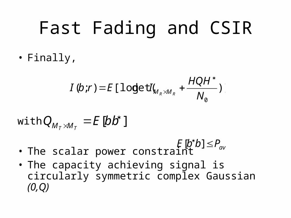
Fast Fading and CSIR
• Finally,
with
• The scalar power constraint• The capacity achieving signal is circularly
symmetric complex Gaussian (0,Q)
)]det([log);(0N
HQHIErbI
RR MM
][ bbEQ
TT MM
avPbbE ][
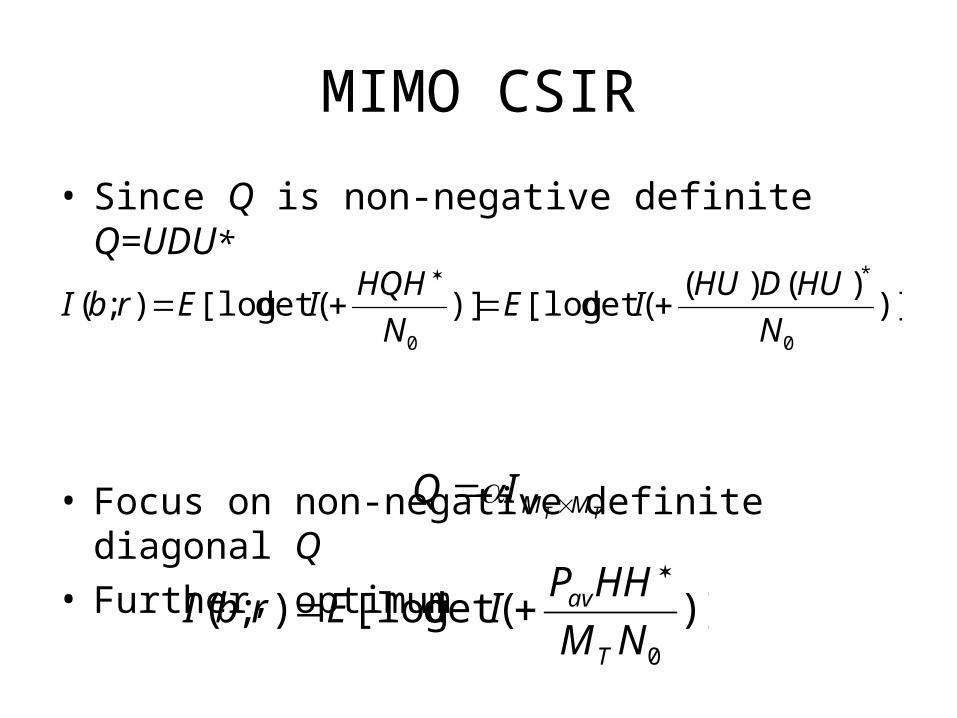
MIMO CSIR
• Since Q is non-negative definite Q=UDU*
• Focus on non-negative definite diagonal Q• Further, optimum
)])()(
det([log)]det([log);(0
*
0 N
HUDHUIE
N
HQHIErbI
TT MMIQ
)]det([log);(0NM
HHPIErbI
T
av

Rayleigh Fading MIMO
• CSIR achievable rate
• Complex Gaussian distribution on H• The square matrix W=HH*
– Wishart distribution– Non negative definite– Distribution of eigenvalues
)]det([log);(0NM
HHPIErbI
T
av
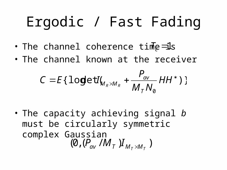
Ergodic / Fast Fading
• The channel coherence time is• The channel known at the receiver
• The capacity achieving signal b must be
circularly symmetric complex Gaussian
1cT
)}det({log0
HH
NM
PIEC
T
avMM RR
))/(,0(TT MMTav IMP

Slow Fading MIMO
• A channel realization is valid for the duration of the code (or transmission)
• There is a non zero probability that the channel can not sustain any rate
• Shannon capacity is zero

Slow Fading Channel
• If the coherence time Tc is the block length
• The outage probability with CSIR only
with and
)det(log);(0
*
N
QHHIbrI RTTR
RR
MMMMMM
])det(Pr[loginf),(0
RN
HQHIPR
RR MMQ
avout
avPbbE ][ ][ bbEQ

Slow Fading
• Since
• Diagonal Q is optimum• Conjecture: optimum Q is
])det(Pr[log])det(Pr[log0
*
0
RN
HHUQUIR
N
HQHI
RRRR MMMM
0
0
1
1
1
m
PQ av
opt

Example
• Slow fading SIMO, • Then and
• Scalar
avopt PQ
])1Pr[log(])det(Pr[log0
*
0
RN
HHPR
N
HQHI av
MM RR
1TM
ddistribute is 2* HH
)(),(
)1(
0
1
out
0
R
P
eN
uM
av M
dueu
PR
av
R
R

Example
• Slow fading MISO,• The optimum
• The outage
1RM
Tmmav
opt MmIm
PQ somefor
)(])1Pr[log(
)1(
0
1
0
*
0
m
dueu
RmN
HHP
av
R
P
emN
um
av

Diversity and Multiplexing for MIMO
• The capacity increase with SNR
• The multiplexing gain
)1log(k
SNRkC
)log(
)(lim
SNR
SNRCr
SNR

Diversity versus Multiplexing
• The error measure decreases with SNR increase
• The diversity gain
• Tradeoff between diversity and multiplexing– Simple in single link/antenna fading channels
dSNR
)log(
))(log(lim
SNR
SNRd out
SNR
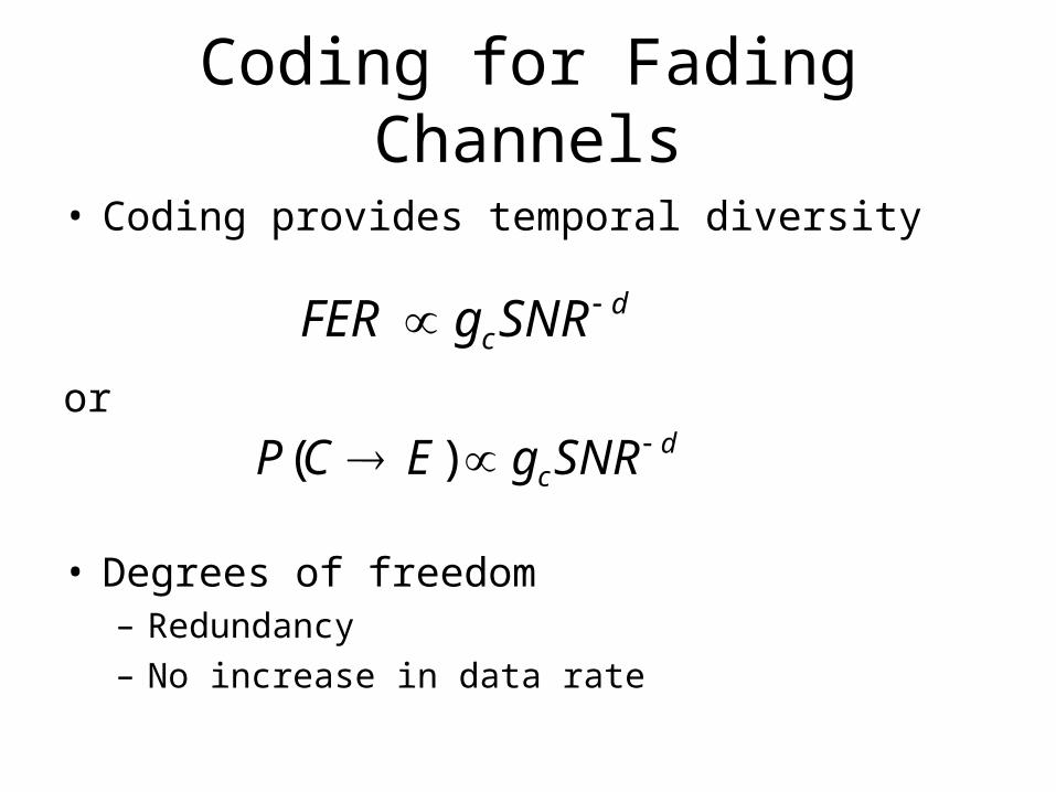
Coding for Fading Channels
• Coding provides temporal diversity
or
• Degrees of freedom – Redundancy– No increase in data rate
dcSNRgFER
dcSNRgECP )(

M versus D
(0,MRMT)
(min(MR,MT),0)
Multiplexing Gain
Div
ers
ity G
ain