Water Resources and - Academic Journals

International Journal of

Water Resources and

Environmental

Engineering

Volume 6 Number 3 March, 2014

www.academicjournals.org/ijwree

ISSN-2141-6613

ABOUT IJWREE

The International Journal of Water Resources and Environmental Engineering is published monthly (one volume per year) by Academic Journals.

International Journal of Water Resources and Environmental Engineering (IJWREE) is an open access journal that provides rapid publication (monthly) of articles in all areas of the subject such as waste management, ozone depletion, Kinetic Processes in Materials, strength of building materials, global warming etc. The Journal welcomes the submission of manuscripts that meet the general criteria of significance and scientific excellence. Papers will be published shortly after acceptance. All articles published in IJWREE are peer-reviewed.

Contact Us

Editorial Office: [email protected]

Help Desk: [email protected]

Website: http://www.academicjournals.org/journal/IJWREE

Submit manuscript online http://ms.academicjournals.me/

mailto:[email protected]

mailto:[email protected]

http://www.academicjournals.org/journal/IJWREE

http://ms.academicjournals.me/

http://ms.academicjournals.me/

Editors

Prof. T. Murugesan Universiti Teknologi PETRONAS, Malaysia Specialization: Chemical Engineering Malaysia.

Dr. Sadek Z Kassab Mechanical Engineering Department, Faculty of Engineering, Alexandria University, Alexandria, Egypt At Present: Visting Professor,Mechanical Engineering Department,Faculty of Engineering & Technology, Arab Academy for Science,Technology & Maritime Transport, Alexandria, Egypt Specialization: Experimental Fluid Mechanics Egypt.

Dr. Minghua Zhou College of Environmental Science and Engineering, Nankai University Specialization: Environmental Engineering (Water Pollution Control Technologies) China.

Dr. Hossam Hamdy Elewa National Authority for Remote Sensing and Space Sciences (NARSS), Cairo, Egypt. Specialization: Hydrogeological and Hydrological applications of Remote Sensing and GIS Egypt.

Dr. Mohamed Mokhtar Mohamed Abdalla Benha University Specialization: Surface & Catalysis Egypt.

Dr. Michael Horsfall Jnr University of Port Harcourt Specialization: (chemistry) chemical speciation and adsorption of heavy metals Nigeria.

Engr. Saheeb Ahmed Kayani Department of Mechanical Engineering, College of Electrical and Mechanical Engineering, National University of Sciences and Technology, Islamabad, Pakistan.

Editorial Board

Prof. Hyo Choi Dept. of Atmospheric Environmental Sciences College of Natural Sciences Gangneung-Wonju National University Gangneung city, Gangwondo 210-702 Specialization: Numerical forecasting of Rainfall and Flood, Daily hydrological forecasting , Regional & Urban climate modelling -wind, heat, moisture, water Republic of Korea

Dr. Adelekan, Babajide A. Department of Agricultural Engineering, College of Engineering and Technology, Olabisi Onabanjo Specialization: Agricultural and Environmental Engineering, Water Resources Engineering, Other Engineering based Water-related fields. Nigeria

Dr. Rais Ahmad Department of Applied Chemistry F/O Engineering & Technology Aligarh Muslim University specialization: Environmetal Chemistry India

Dr. Venkata Krishna K. Upadhyayula Air Force Research labs, Tyndall AFB, Panama City, FL, USA Specialization: Environmental Nanotechnology, Biomaterials, Pathogen Sensors, Nanomaterials for Water Treatment Country: USA

Dr. R. Parthiban Sri Venkateswara College of Engineering Specialization - Environmental Engineering India

Dr. Haolin Tang State Key Laboratory of Advanced Technology for Materials Synthesis and Processing, Wuhan University of Technology Specialization: Hydrogen energy, Fuel cell China

Dr. Ercument Genc Mustafa Kemal University (Aquaculture Department Chairman, Faculty of Fisheries, Department of Aquaculture, Branch of Fish Diseases, Mustafa Kemal University,31200,Iskenderun, Hatay, Turkey) Specialization: Environmental (heavy metal), nutritional and hormonal pathologies, Parasitic infections prevalences and their histopathologies in aquatic animals Turkey

Dr. Weizhe An KLH Engineers, Inc., Pittsburgh, PA, USA. Specialization: Stormwater management, urban hydrology, watershed modeling, hydrological engineering, GIS application in water resources engineering. USA

Dr. T.M.V. Suryanarayana Water Resources Engineering and Management Institute, Faculty of Tech. and Engg.,The Maharaja Sayajirao University of Baroda, Samiala - 391410, Ta. & Dist.:Baroda. Specialization: Water Resources Engineering & Management, Applications of Soft Computing Techniques India

Dr. Hedayat Omidvar National Iranian Gas Company Specialization: Gas Expert Iran

Dr. Ta Yeong Wu School of Engineering Monash University Jalan Lagoon Selatan, Bandar Sunway, 46150, Selangor Darul Ehsan Specialization: Biochemical Engineering; Bioprocess Technology; Cleaner Production; Environmental Engineering; Membrane Technology. Malaysia.

International Journal of Medicine and Medical Sciences

International Journal of Water Resources and Environmental Engineering

Table of Contents: Volume 6 Number 3 March 2014

ARTICLES

Research Articles Flood hazard assessment of River Dep floodplains in North-Central 99 Nigeria Rose E. Daffi, Johnson A. Otun and Abubakar Ismail Catchment dynamics and its impact on runoff generation: 105 Coupling watershed modelling and statistical analysis to detect catchment responses Negash Wagesho Heavy metals assessment of private drinking water supplies 112 in Ibadan, Nigeria and associated health risks B. A. Adelekan and Oguntoso N.

Vol. 6(3), pp. 98-105, March, 2014

DOI: 10.5897/IJWREE2013.0465

Article Number: 16BD64A4674

ISSN 2141-6613

Copyright © 2014

Author(s) retain the copyright of this article

http://www.academicjournals.org/IJWREE


Full Length Research Paper

Simulation of rainfall runoff process for Khartoum State (Sudan) using remote sensing and geographic

information systems (GIS)

A. Aldoma and M. Y. Mohamed*

Faculty of agriculture AlzaiemAlazhary University, Sudan

Received 5 December, 2013; Accepted 20 February, 2014

Using geographic information systems (GIS) and remote sensing integration to determine runoff caused due to rainfall from watershed has performed increasingly attention in recent years. This study was conducted in the Khartoum State. Curve Number (CN) method was applied for estimating the runoff depth in the watershed. Hydrologic soil group and land use maps were generated in GIS Environment. Hydrologic soil groups and land use maps were used to generate the CN map. Soil Conservation Services-Curve number (SCS-CN) method was followed to estimate runoff for the watershed. It was found that the model can predict runoff reasonably well. It could be concluded that the SCS-CN method can be applied to predict runoff volumes for planning of various conservation measures and for other water resources applications. Key words: Soil Conservation Services-Curve number (SCS-CN), geographic information systems (GIS), remote sensing, runoff estimation

INTRODUCTION Surface runoff is the water flow that occurs when soil is saturated to full capacity and excess water from rain over the land. This is a major component of the water cycle. Rainfall generates runoff, and its occurrence and quantity are dependent on the characteristics of the rainfall event, that is, the intensity, duration and distribution. Apart from these rainfall characteristics, there are numbers of catchment specific factors, which have a direct effect on the occurrence and volume of runoff.

Measured rainfall is one of the most significant input data in applying the hydrological models for runoff estimations. Unfortunately, the distribution of rainfall usually varies significantly in both space and time. Therefore, the limited number of rainfall stations in the

catchment can have a major impact on the accuracy of runoff estimations. The accurate estimation of the spatial distribution of rainfall therefore requires a very dense rainfall network, which involves high installation and operational costs.

Remote sensing can provide measurements of many of the hydrologic variables used in hydrologic applications, either as direct measurements comparable to traditional forms, or as entirely new data set. The pixel format of digital remote sensing data makes it suitable to merge it with geographic information system (GIS).

Most of the previous work on adapting remote sensing to hydrologic modeling has involved the Natural Resources Conservation Service runoff Curve Number

*Corresponding author. Email: [email protected]

Author(s) agree that this article remain permanently open access under the terms of the Creative Commons Attribution

License 4.0 International License

http://www.answers.com/topic/water

http://www.answers.com/topic/rain

http://www.answers.com/topic/hydrologic-cycle

http://creativecommons.org/licenses/by/4.0/deed.en_US


(CN) model. This involvement used remote sensing data as a substitute for land cover maps which had been obtained by conventional means.

The GIS technology provides suitable alternatives for efficient management of large and complex databases; it is used in hydrologic modeling to facilitate processing, management and interpretation of hydrologic data.

Several studies have been done to incorporate GIS in to hydrologic modeling of watersheds. The traditional method for establishing CN on small watersheds includes field surveys and interpretations of aerial photographs. For large drainage basins, field surveys are prohibitively expensive and an excessive number of aerial photographs may be required for complete coverage. A further disadvantage of conventional techniques may be the infrequency of the surveys and the consequent failure to account for changes in vegetative cover and land use.

Land use is an important characteristic of the runoff process that affects infiltration, erosion, and evapotranspiration. Hydrologic models, distributed models in particular, need specific data on land use and its location within the basin. Remote sensing can provide measurements of many of the hydrologic variables used in hydrologic and environmental model.

Rainfall-runoff modeling is a very important topic of research that can be utilized for management and control of water resources. Where there is lack of important elements such as digital land use map, digital curve number map, hydrological soil groups map and digital runoff map, these types of maps are very useful in hydrological investigations. In addition, future predictions with different scenarios can be undertaken by rainfall-runoff modeling.

The integration of remote sensing and GIS has been widely applied and has been recognized as a powerful and effective tool in estimating and evaluating rainfall; therefore the main aim of the present study is to apply a rainfall-runoff model using GIS and remote sensing techniques to simulate the rainfall-runoff process and create digital runoff map for the study area using SCS-CN method.

Nowadays, modeling has become a common practice in every field of endeavor, and runoff modeling is no exception (Donigian, 1995). The main reason behind the using of modeling in general is the limitations of the techniques used in measuring and observing the various components of hydrological systems (Beven, 2001). Also using hydrologic models will increase our understanding and explanation of the natural phenomena and its dynamic interactions with the surrounding systems (that is, climatic terrestrial, pedologic, lithologic and hydrologic systems) (Chiew, 1994). However, under some conditions, predictions can be made in deterministic or probabilistic sense.

Another use of modeling is to predict how the system will respond to the future alternative conditions and actions (Donigian et al., 1995; Linsley, 1982) summarized

Aldoma and Mohamed 99 the principal purposes for which hydrological model have or can be employed. In general they can be used for hydrologic research purposes, for forecasting and prediction of stream flow, and for engineering and statistical applications (record extension, operational simulation, data fill-in, and data revision).

Detailed analysis of flood hydrograph has special importance in flood mitigation, flood forecasting and/or establishing flows for many structures which must convey floodwaters (Linsley, 1982). Rainfall-Runoff modeling covers a wide range of applications and practices. This can be divided into two main groups, viz: flood studies (planning and designing new hydraulic structure, operating and/or evaluatingexisting hydraulic structures, preparing for and responding to flood, flood damage reduction, and regulating flood plain activities), and storage studies (catchment and reservoir yield analysis, and water resource potential) (Blandford and Meadows, 1990; Chiew, 1994; Connolly, 1995).

The Soil Conservation Service - curve number (SCS-CN) method has its origins in the unit hydrograph approach to rainfall-runoff modeling. The unit hydrograph approach always requires a method for predicting how much of the rainfall contributes to the storm runoff. The SCS-CN method arose out of the empirical analysis of runoff from small catchments and hill slope plots monitored by the USDA. The Curve Number method (SCS, 1972),also known as the Hydrologic Soil Cover Complex Method, is a versatile and widely used procedure for runoff estimation. In this method, runoff producing capability is expressed by a numerical value varying between 0 to 100.

METHODOLOGY

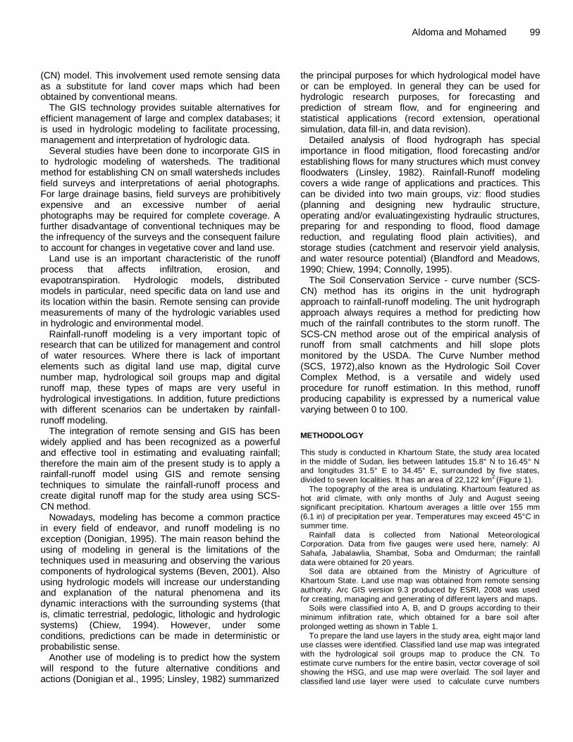
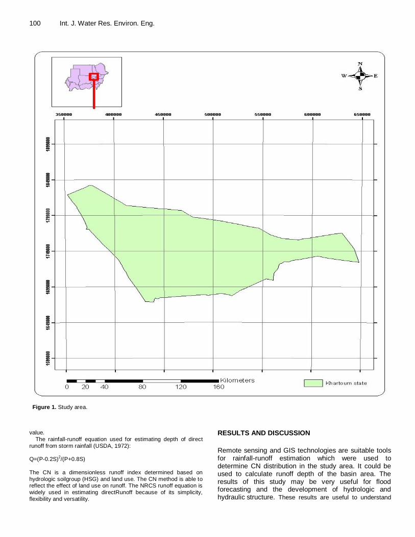
This study is conducted in Khartoum State, the study area located in the middle of Sudan, lies between latitudes 15.8° N to 16.45° N and longitudes 31.5° E to 34.45° E, surrounded by five states, divided to seven localities. It has an area of 22,122 km

2 (Figure 1).

The topography of the area is undulating. Khartoum featured as hot arid climate, with only months of July and August seeing significant precipitation. Khartoum averages a little over 155 mm (6.1 in) of precipitation per year. Temperatures may exceed 45°C in summer time.

Rainfall data is collected from National Meteorological Corporation. Data from five gauges were used here, namely: Al Sahafa, Jabalawlia, Shambat, Soba and Omdurman; the rainfall data were obtained for 20 years.

Soil data are obtained from the Ministry of Agriculture of Khartoum State. Land use map was obtained from remote sensing

authority. Arc GIS version 9.3 produced by ESRI, 2008 was used for creating, managing and generating of different layers and maps.

Soils were classified into A, B, and D groups according to their minimum infiltration rate, which obtained for a bare soil after prolonged wetting as shown in Table 1.

To prepare the land use layers in the study area, eight major land use classes were identified. Classified land use map was integrated with the hydrological soil groups map to produce the CN. To estimate curve numbers for the entire basin, vector coverage of soil showing the HSG, and use map were overlaid. The soil layer and classified land use layer were used to calculate curve numbers

http://en.wikipedia.org/wiki/Arid_climate

100 Int. J. Water Res. Environ. Eng.

Figure 1. Study area.

value. The rainfall-runoff equation used for estimating depth of direct

runoff from storm rainfall (USDA, 1972): Q=(P-0.2S)

2/(P+0.8S)

The CN is a dimensionless runoff index determined based on hydrologic soilgroup (HSG) and land use. The CN method is able to reflect the effect of land use on runoff. The NRCS runoff equation is widely used in estimating directRunoff because of its simplicity, flexibility and versatility.

RESULTS AND DISCUSSION

Remote sensing and GIS technologies are suitable tools for rainfall-runoff estimation which were used to determine CN distribution in the study area. It could be used to calculate runoff depth of the basin area. The results of this study may be very useful for flood forecasting and the development of hydrologic and hydraulic structure. These results are useful to understand

Aldoma and Mohamed 101

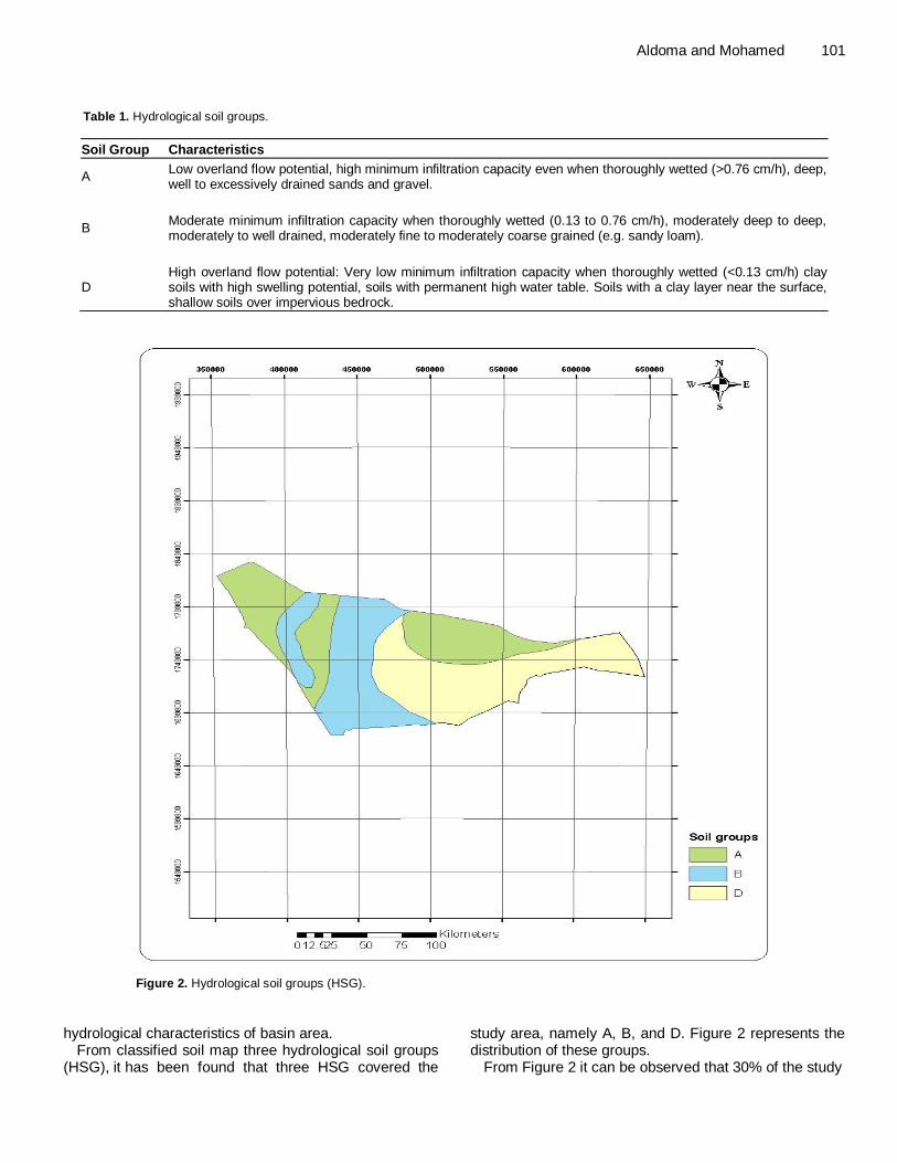
Table 1. Hydrological soil groups.

Soil Group Characteristics

A Low overland flow potential, high minimum infiltration capacity even when thoroughly wetted (>0.76 cm/h), deep, well to excessively drained sands and gravel.

B Moderate minimum infiltration capacity when thoroughly wetted (0.13 to 0.76 cm/h), moderately deep to deep, moderately to well drained, moderately fine to moderately coarse grained (e.g. sandy loam).

D High overland flow potential: Very low minimum infiltration capacity when thoroughly wetted (<0.13 cm/h) clay soils with high swelling potential, soils with permanent high water table. Soils with a clay layer near the surface, shallow soils over impervious bedrock.

Figure 2. Hydrological soil groups (HSG).

hydrological characteristics of basin area.

From classified soil map three hydrological soil groups (HSG), it has been found that three HSG covered the

study area, namely A, B, and D. Figure 2 represents the distribution of these groups.

From Figure 2 it can be observed that 30% of the study


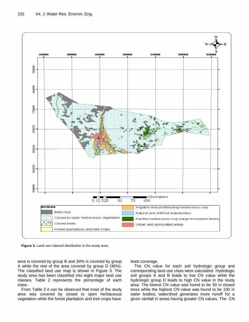
Figure 3. Land use classed distribution in the study area.

area is covered by group B and 34% is covered by group A while the rest of the area covered by group D (36%). The classified land use map is shown in Figure 3. The study area has been classified into eight major land use classes. Table 2 represents the percentage of each class.

From Table 2 it can be observed that most of the study area was covered by closed to open herbaceous vegetation while the forest plantation and tree crops have

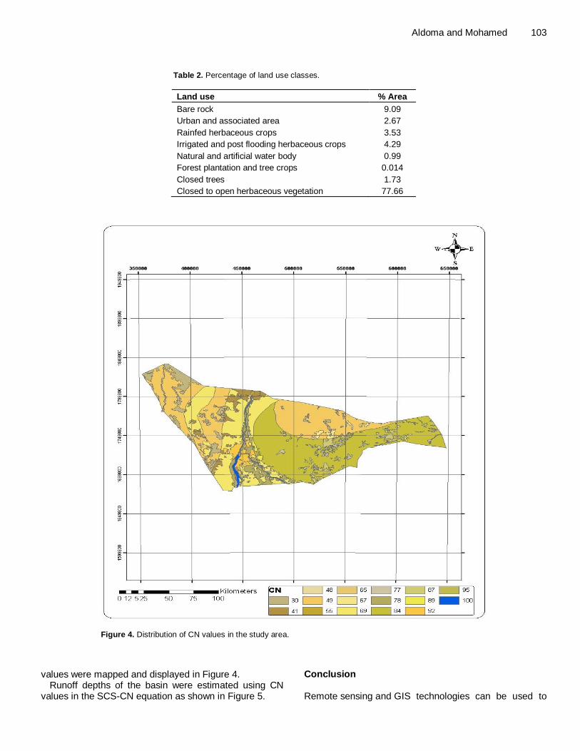
least coverage. The CN value for each soil hydrologic group and

corresponding land use class were calculated. Hydrologic soil groups A and B leads to low CN value while the hydrologic group D leads to high CN value in the study area. The lowest CN value was found to be 30 in closed trees while the highest CN value was found to be 100 in water bodies; watershed generates more runoff for a given rainfall in areas having greater CN values. The CN

Aldoma and Mohamed 103

Table 2. Percentage of land use classes.

Land use % Area

Bare rock 9.09

Urban and associated area 2.67

Rainfed herbaceous crops 3.53

Irrigated and post flooding herbaceous crops 4.29

Natural and artificial water body 0.99

Forest plantation and tree crops 0.014

Closed trees 1.73

Closed to open herbaceous vegetation 77.66

Figure 4. Distribution of CN values in the study area.

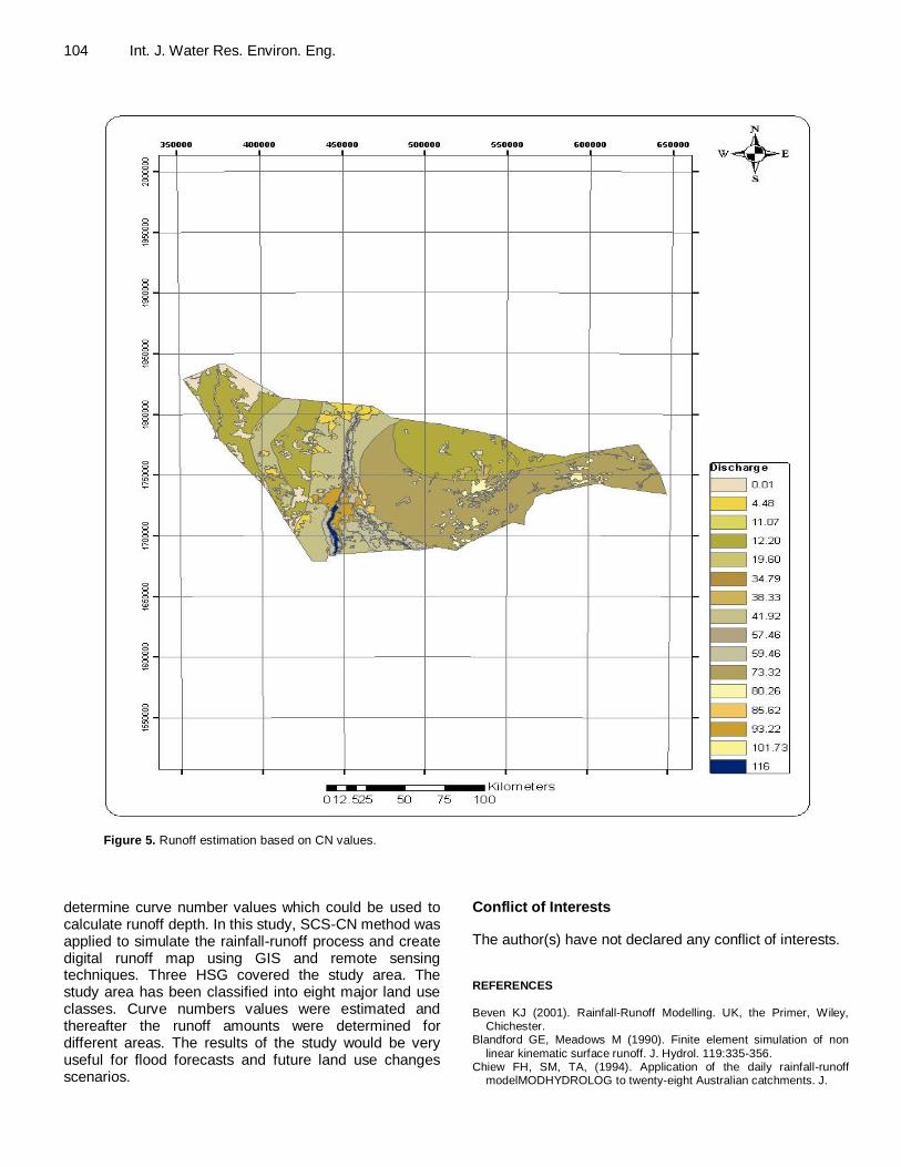
values were mapped and displayed in Figure 4. Runoff depths of the basin were estimated using CN

values in the SCS-CN equation as shown in Figure 5.

Conclusion Remote sensing and GIS technologies can be used to


Figure 5. Runoff estimation based on CN values.

determine curve number values which could be used to calculate runoff depth. In this study, SCS-CN method was applied to simulate the rainfall-runoff process and create digital runoff map using GIS and remote sensing techniques. Three HSG covered the study area. The study area has been classified into eight major land use classes. Curve numbers values were estimated and thereafter the runoff amounts were determined for different areas. The results of the study would be very useful for flood forecasts and future land use changes scenarios.

Conflict of Interests

The author(s) have not declared any conflict of interests. REFERENCES

Beven KJ (2001). Rainfall-Runoff Modelling. UK, the Primer, Wiley, Chichester.

Blandford GE, Meadows M (1990). Finite element simulation of non

linear kinematic surface runoff. J. Hydrol. 119:335-356. Chiew FH, SM, TA, (1994). Application of the daily rainfall-runoff

modelMODHYDROLOG to twenty-eight Australian catchments. J.

Hydrol. 153:383-416. Connolly RD, SDM (1995). Distributed parameter hydrology model

(ANSWERS) applied to a range of catchment scales using rainfall

simulator data I: Infiltration modelling and parameter measurement. Donigian AS, Bicknell BR, Imhof JC (1995). Hydrological Simulation

Program – Fortran (HSPF). Colorado, Water Resources Pubs

Aldoma and Mohamed 105 Linsley RK, Kohler MA, JL, Paulhus H (1982). Hydrology for Engineers

New York, McGraw-Hill Book Co. SCS (1972). National Engineering Handbook. Washington, D.C.,

Department of Agriculture, U.S.

Vol. 6(3), pp. 106-111, March, 2014

DOI: 10.5897/IJWREE2013.0374

Article Number: DAC15B846747

ISSN 2141-6613

Copyright © 2014





Classification of transmissivity magnitude and variation in calcarious soft rocks of Bhaskar Rao Kunta

Watershed, Nalgonda District, India

K. Srinivasa Reddy

ICAR-Central Research Institute for Dryland Agriculture, Hyderabd-59, India.

Received 5 December, 2012; Accepted 2 July, 2013

Pumping test was used for the appraisal and evaluation of groundwater potential and design of well. Pumping tests of the calcarious sedimentary rocks of Bhaskar Rao kunta watershed area were carried out for twenty five selected bore wells for quantitative understanding of the groundwater for crop water requirement and groundwater use efficiency. The tests were carried out independently for short duration under constant rate conditions. The acquisition of the drawdown data was interpreted by Jacob straight line method. The results of transmissivity vary from 2.67 to 236.9 m

2/day with mean of 37

m2/day, whereas the specific capacity varies from 5.47 to 451.63 m

3/d/m with a mean of 76 m

3/d/m.

Spatial variation of transmissivity values was further analyzed using statistical testing and Krasny’s classification systems; from the results of the statistical testing, 72% of the wells were under covered background transmissivity anomalies; 12% under positive anomalies; 8%, negative anomalies and remaining 8%, positive extreme anomalies. From the results of Krasny’s classification system, 12% of the wells was under high magnitude (withdrawals of lesser regional importance), 40% of wells was under intermediate magnitude (withdrawals for local water supply), 48% was under low magnitude (smaller withdrawals for local water supply) and 100% of the wells was under covered moderate variations (fairly heterogeneous hydrogeological environment). Spatial variation of transmissivity magnitude and variation was identified as best useful in management practices. Key words: Transmissivity, magnitude, variation, statistical testing, Krasny’s classification.

INTRODUCTION Quantitative understanding of most problems in hydrogeology (Ramakrishna, 1998), determination and evaluation of aquifer parameters of transmissivity and storage coefficient from aquifer test data is a continual field research (Birpinar, 2003); it is field–scale prediction (Illman and Tartakovsky, 2006) and integral part of assessment and management of groundwater study

(Sarwade et al., 2007; Mayooran et al., 2011; Sudher Kumar et al., 2012). Generally, there are two types of pumping tests evaluation methods for determining aquifer parameters: (i) drawdown and (ii) recovery. In the present study, only drawdown test was conducted.

The present study was done in a semi-arid region of Bhaskar Rao kunta watershed area (40 km

2), which is a

E-mail: [email protected], Tel: +91 9866673218. Author(s) agree that this article remain permanently open access under the terms of the Creative Commons Attribution




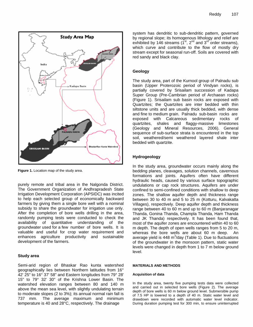
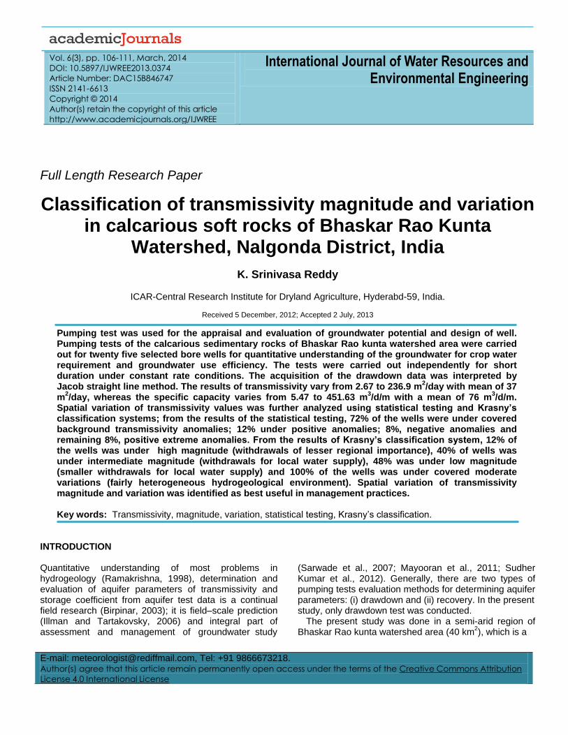
Figure 1. Location map of the study area. purely remote and tribal area in the Nalgonda District. The Government Organization of Andhrapradesh State Irrigation Development Corporation (APSIDC) was incited to help each selected group of economically backward farmers by giving them a single bore well with a nominal subsidy to share the groundwater for irrigation use only. After the completion of bore wells drilling in the area, randomly pumping tests were conducted to check the availability of quantitative understanding of the groundwater used for a few number of bore wells. It is valuable and useful for crop water requirement and enhances agriculture productivity and sustainable development of the farmers. Study area Semi-arid region of Bhaskar Rao kunta watershed geographically lies between Northern latitudes from 16° 42' 25" to 16° 37' 58" and Eastern longitudes from 79° 28' 15" to 79° 32' 30" of the Krishna Lower Basin. The watershed elevation ranges between 80 and 140 m above the mean sea level, with slightly undulating terrain to moderate slopes (2 to 3%); its annual normal rain fall is 737 mm. The average maximum and minimum temperature is 40 and 28°C, respectively. The drainage

Reddy 107 system has dendritic to sub-dendritic pattern, governed by regional slope; its homogenous lithology and relief are exhibited by 146 streams (1

st, 2

nd and 3

rd order streams),

which curve and contribute to the flow of mostly dry stream except for seasonal run-off. Soils are covered with red sandy and black clay. Geology The study area, part of the Kurnool group of Palnadu sub basin (Upper Proterozoic period of Vindyan rocks), is partially covered by Srisailam succession of Kadapa Super Group (Pre-Cambrian period of Archaean rocks) (Figure 1). Srisailam sub basin rocks are exposed with Quartzites; the Quartzites are inter bedded with thin siltstone units and are usually thick bedded, with dense and fine to medium grain. Palnadu sub-basin rocks are exposed with Calcareous sedimentary rocks of quartzites, shales and flaggy-massive limestones (Geology and Mineral Resources, 2006). General sequence of sub-surface strata is encountered in the top soil, weathered/semi weathered layered shale inter bedded with quartzite. Hydrogeology In the study area, groundwater occurs mainly along the bedding planes, cleavages, solution channels, cavernous formations and joints. Aquifers often have different hydraulic heads, caused by various surface topographic undulations or cap rock structures. Aquifers are under confined to semi-confined conditions with shallow to deep zones. The shallow aquifer depth and thickness range between 30 to 40 m and 5 to 25 m (Kotturu, Kalvakatta Villages), respectively. Deep aquifer depth and thickness range between 40 to 60 m and up to 60 m (Banjaranagar Thanda, Gonina Thanda, Champla Thanda, Ham Thanda and JK Thanda) respectively. It has been found that, most of the aquifer zones are encountered within 40 to 60 m depth. The depth of open wells ranges from 5 to 20 m, whereas the bore wells are about 60 m deep. An average yield is 448 m

3/day (Table 1). Due to fluctuations

of the groundwater in the monsoon pattern, static water levels were changed in depth from 1 to 7 m below ground level. MATERIALS AND METHODS

Acquisition of data

In the study area, twenty five pumping tests data were collected and carried out in selected bore wells (Figure 2). The average depth of bore wells is 60 m below ground level. Submersible pump of 7.5 HP is lowered to a depth of 40 m. Static water level and drawdown were recorded with automatic water level indicator. During duration pumping test for 300 min, to ensure uninterrupted


Table 1. Results of aquifer parameters of twenty five bore wells.

Well

No.

Pumping

duration (min)

Static water

levels (m)

Drawdown (m) Discharge

(m3/day )

Specific capacity

(m3/d/m)

Transmissivity

(m2/day) Min. Max.

1 300 5 16 29.8 130 4.36 3.65

2 300 1 2.9 4.9 726 148.16 69.98

3 300 5.8 13.3 26.95 473 17.55 16.98

4 300 6 4.25 11.4 453 39.81 16.59

5 300 1 2.5 29.6 162 5.47 2.67

6 300 1 2 13.9 466 33.53 12.91

7 300 0.2 2.6 14.55 602 41.37 16.22

8 300 6 1.15 2.85 971 451.63 236.9

9 300 7.15 1.35 6.75 773 114.52 54.17

10 300 1.5 7.65 15.76 456 29 9.73

11 300 1.3 1.4 2.3 869 377.83 186.15

12 300 6.8 9.45 22.58 359 15.9 7.07

13 300 0.2 18.6 35 272 7.77 5.41

14 300 6.2 12.3 28.3 188 6.76 6.53

15 300 2.1 1.6 4.55 727 199.18 102.39

16 300 4 16.2 31 250 8.06 4.82

17 300 6 0.15 13.5 227 16.81 5.21

18 300 1.2 2.3 5.4 512 94.81 52.13

19 300 0.2 2.5 6.6 455 68.94 26.01

20 300 3.5 0.2 12.7 557 43.86 8.43

21 300 7 8.2 25.2 235 9.36 10.26

22 300 7 0.8 12 173 14.42 6.14

23 300 6 14.1 24 225 9.38 5.87

24 300 6 0.6 7.6 413 54.34 20.43

25 300 6.2 1.7 13.3 216 17 5.31

Minimum 0.20 0.15 2.30 130.00 5.47 2.67

Maximum 7.15 18.60 29.6 971.00 451.63 236.90

Mean 3.89 5.33 15.45 448.33 76.06 37.01

Standard Deviation 2.67 5.66 9.93 233.54 115.76 59.55

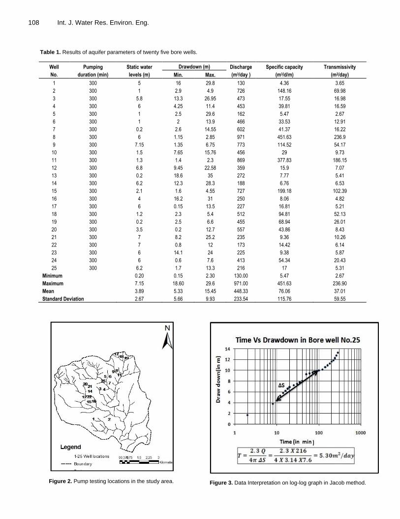
Figure 2. Pump testing locations in the study area.

Figure 3. Data Interpretation on log-log graph in Jacob method.

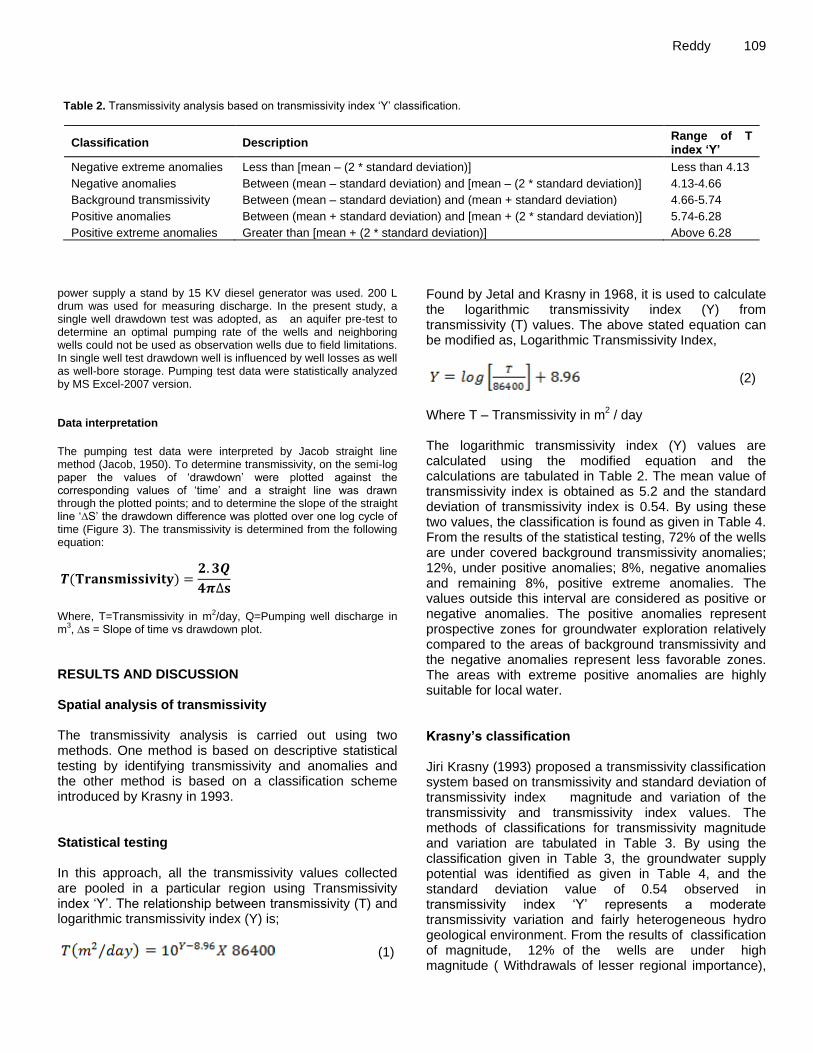
Reddy 109 Table 2. Transmissivity analysis based on transmissivity index ‘Y’ classification.

Classification Description Range of T index ‘Y’

Negative extreme anomalies Less than [mean – (2 * standard deviation)] Less than 4.13

Negative anomalies Between (mean – standard deviation) and [mean – (2 * standard deviation)] 4.13-4.66

Background transmissivity Between (mean – standard deviation) and (mean + standard deviation) 4.66-5.74

Positive anomalies Between (mean + standard deviation) and [mean + (2 * standard deviation)] 5.74-6.28

Positive extreme anomalies Greater than [mean + (2 * standard deviation)] Above 6.28

power supply a stand by 15 KV diesel generator was used. 200 L drum was used for measuring discharge. In the present study, a single well drawdown test was adopted, as an aquifer pre-test to determine an optimal pumping rate of the wells and neighboring wells could not be used as observation wells due to field limitations. In single well test drawdown well is influenced by well losses as well as well-bore storage. Pumping test data were statistically analyzed by MS Excel-2007 version. Data interpretation

The pumping test data were interpreted by Jacob straight line method (Jacob, 1950). To determine transmissivity, on the semi-log paper the values of ‘drawdown’ were plotted against the corresponding values of ‘time’ and a straight line was drawn through the plotted points; and to determine the slope of the straight line ‘∆S’ the drawdown difference was plotted over one log cycle of time (Figure 3). The transmissivity is determined from the following equation:

𝑻(𝐓𝐫𝐚𝐧𝐬𝐦𝐢𝐬𝐬𝐢𝐯𝐢𝐭𝐲) =𝟐.𝟑𝑸

𝟒𝝅∆𝐬

Where, T=Transmissivity in m

2/day, Q=Pumping well discharge in

m3, ∆s = Slope of time vs drawdown plot.

RESULTS AND DISCUSSION Spatial analysis of transmissivity The transmissivity analysis is carried out using two methods. One method is based on descriptive statistical testing by identifying transmissivity and anomalies and the other method is based on a classification scheme introduced by Krasny in 1993. Statistical testing In this approach, all the transmissivity values collected are pooled in a particular region using Transmissivity index ‘Y’. The relationship between transmissivity (T) and logarithmic transmissivity index (Y) is;

(1)

Found by Jetal and Krasny in 1968, it is used to calculate the logarithmic transmissivity index (Y) from transmissivity (T) values. The above stated equation can be modified as, Logarithmic Transmissivity Index,

(2)

Where T – Transmissivity in m

2 / day

The logarithmic transmissivity index (Y) values are calculated using the modified equation and the calculations are tabulated in Table 2. The mean value of transmissivity index is obtained as 5.2 and the standard deviation of transmissivity index is 0.54. By using these two values, the classification is found as given in Table 4. From the results of the statistical testing, 72% of the wells are under covered background transmissivity anomalies; 12%, under positive anomalies; 8%, negative anomalies and remaining 8%, positive extreme anomalies. The values outside this interval are considered as positive or negative anomalies. The positive anomalies represent prospective zones for groundwater exploration relatively compared to the areas of background transmissivity and the negative anomalies represent less favorable zones. The areas with extreme positive anomalies are highly suitable for local water. Krasny’s classification Jiri Krasny (1993) proposed a transmissivity classification system based on transmissivity and standard deviation of transmissivity index magnitude and variation of the transmissivity and transmissivity index values. The methods of classifications for transmissivity magnitude and variation are tabulated in Table 3. By using the classification given in Table 3, the groundwater supply potential was identified as given in Table 4, and the standard deviation value of 0.54 observed in transmissivity index ‘Y’ represents a moderate transmissivity variation and fairly heterogeneous hydro geological environment. From the results of classification of magnitude, 12% of the wells are under high magnitude ( Withdrawals of lesser regional importance),

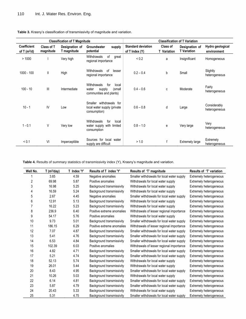
110 Int. J. Water Res. Environ. Eng. Table 3. Krasny’s classification of transmissivity of magnitude and variation.

Classification of T Magnitude Classification of T Variation

Coefficient

of T (m2/d)

Class of T magnitude

Designation of T magnitude

Groundwater supply potential

Standard deviation

of T Index (Y)

Class of

T Variation

Designation of T Variation

Hydro geological

environment

> 1000 I Very high Withdrawals of great regional importance

< 0.2 a Insignificant Homogeneous

1000 - 100 II High Withdrawals of lesser regional importance

0.2 – 0.4 b Small Slightly heterogeneous

100 - 10 III Intermediate Withdrawals for local water supply (small communities and plants)

0.4 – 0.6 c Moderate Fairly heterogeneous

10 - 1 IV Low Smaller withdrawals for local water supply (private consumption)

0.6 – 0.8 d Large Considerably heterogeneous

1 - 0.1 V Very low Withdrawals for local water supply with limited consumption

0.8 – 1.0 e Very large Very heterogeneous

< 0.1 VI Imperceptible Sources for local water supply are difficult

> 1.0 f Extremely large Extremely heterogeneous

Table 4. Results of summary statistics of transmissivity index (Y), Krasny’s magnitude and variation.

Well No. T (m2/day) T Index 'Y' Results of T index 'Y' Results of ‘T’ magnitude Results of ‘T’ variation

1 3.65 4.59 Negative anomalies Smaller withdrawals for local water supply Extremely heterogeneous

2 69.98 5.87 Positive anomalies Withdrawals for local water supply Extremely heterogeneous

3 16.98 5.25 Background transmissivity Withdrawals for local water supply Extremely heterogeneous


5 2.67 4.45 Negative anomalies Smaller withdrawals for local water supply Extremely heterogeneous



8 236.9 6.40 Positive extreme anomalies Withdrawals of lesser regional importance Extremely heterogeneous

9 54.17 5.76 Positive anomalies Withdrawals for local water supply Extremely heterogeneous

10 9.73 5.01 Background transmissivity Smaller withdrawals for local water supply Extremely heterogeneous

11 186.15 6.29 Positive extreme anomalies Withdrawals of lesser regional importance Extremely heterogeneous




15 102.39 6.03 Positive anomalies Withdrawals of lesser regional importance Extremely heterogeneous











40% of wells are under intermediate magnitude (withdrawals for local water supply), 48% are under low magnitude (smaller withdrawals for local water supply) and 100% of the wells are under covered moderate variations (fairly heterogeneous hydrogeological environment). CONCLUSION AND RECOMMANDATIONS The study has shown that the transmissivity varies from 2.67 to 236.9 m

2/day (with a mean of 37 m

2/day),

whereas the specific capacity varies from 5.47 to 451.63 m

3/dd/m (with a mean of 76 m

3/d/m). Spatial variation of

transmissivity values was further analyzed using statistical testing and Krasny’s classification systems. From the results of the statistical testing, 72% of the wells are under covered background transmissivity anomalies; the remaining 12, 8 and 8%, under positive, negative and positive extreme anomalies, respectively. From the results of Krasny’s classification system, 48, 40 and 12% of the wells aree under covered low magnitude (smaller withdrawals for local water supply), intermediate magnitude (withdrawals for local water supply) and high magnitude (withdrawals of lesser regional important) respectively. 100% of the wells are under covered moderate variations (fairly heterogeneous hydrogeological environment). Spatial variation of transmissivity magnitude and variation were identified as best useful in management practices and sustainable development of groundwater. A much more appropriate quantitative understanding of the groundwater for a long time pumping test and observation is well required. ACKNOWLEDGEMENT The author is thankful to Executive Engineer, Andhrapradesh State Irrigation Development Corporation (APSIDC), Miryalguda Division, Nalgonda Districts, for collection and utilization of the data. Conflict of Interests

The author(s) have not declared any conflict of interests. REFERENCES Birpinar ME (2003). Aquifer parameter identification and interpretation

with different analytical methods. Water SA, 29 (3):251-256. Geology and mineral resources of Andhra Pradesh (2006). Geological

survey of India, India. Illman WA, Tartakovsky DM (2006). Asymptotic analysis of cross-hole

hydraulic tests in fractured granite. Ground Water 44(4):555-563. Jacob CE (1950). Flow of groundwater in engineering hydraulics: New

York, John Wiley, pp. 321-386.

Reddy 111 Krasny J (1993). ‘Classification of Transmissivity Magnitude and

Variation”, Vol. 31, No. 2-GROUND WATER Mayooran S, Manarathna SP, Gogulan N, Rajapakse RLHL (2011). An

Aquifer Characteristic Analysis For Identifying Groundwater Resource Development Alternatives In The Wet Zone Of Sri Lanka. Civil Engineering Research for Industry, Department of Civil Engineering – University of Moratuwa.

Ramakrishna S (1998). Text book of groundwater. 1st

Edition, K.J.Graphars, Chennai.

Sarwade DV, Singh VS, Puranik SC, Mondal NC (2007). Comparative study of analytical and numerical methods for estimation of aquifers parameters: A case study in basaltic terrain. J. Geol. Soc. India 70(6):1039-1046.

Sudher Kumar M, Srinivas CR, Srinivasa RK, Mondal NC (2012). Evaluation of hydrogeological properties of fractured granitic aquifer in a micro watershed of Kandukuru -Southern India. Int. J. Water Res. Environ. Eng. 4(12):386-396.

Vol. 6(1), pp. 112-120, March, 2014

DOI 10.5897/IJWREE2013. 0464

Article Number: 57876A446748

ISSN 2141-6613

Copyright © 2014





Assessment of noise pollution of two vulnerable sites of Sylhet city, Bangladesh

Nurul Amin1*, Iqbal Sikder1, M. A. Zafor2 and M. A. I. Chowdhury1

1Civil and Environmental Engineering, Shahjalal University of Science and Technology, Sylhet-3100, Bangladesh.

2Civil Engineering, Leading University, Sylhet-3100, Bangladesh.

Received 20 November, 2013 Accepted 7 February, 2014

The study reports the analysis and measurement of the noise levels of CNG refueling Stations and Power Generators of Power Development Board (PDB) induced noise pollution in Sylhet City. For this purpose noise levels have been measured at ten major locations of the city for CNG refueling Stations and in PDB, Kumargaon. Sound levels are measured at different location at different time interval for the respective study locations with the help of a standard Sound meter. It was found that the noise levels for both study locations are much higher that exceed the allowable permissible noise limits. The study suggests that noise path must be controlled by using appropriate sound barriers that can reflect and diffuse noise appropriately and particularly use of sound enclosure can reduce noise level. Key words: Noise pollution, sound level, permissible exposure level.

INTRODUCTION Sylhet city is one of the largest cities of Bangladesh in the northeast portion of the country. Sylhet is the 4

th largest

city of Bangladesh by the population. It covers an area of 26.5 km

2. Day by day the unplanned Urbanization is

going on in this city in a threaten way. Infrastructure is not developing in the right places. As a result of unplanned urbanization, hospitals, schools, colleges and universities like sensitive institutions are building in the noisy area (Shilpy, 2007).

The noise pollution is one of the major problems for developing countries like Bangladesh. Sylhet city is one of the largest cities of Bangladesh in the northeast portion of the country (Shilpy, 2007). The noise originates from human activities, especially the urbanization and the

development of transport and industry. Measuring noise levels and workers' noise exposures is the most important part of a workplace hearing conservation and

noise control program. It helps identify work locations where there are noise problems, employees who may be affected, and where additional noise measurements need to be made (Asthana and Asthana, 2013). Noise is any sound-independent of loudness- that can produce an undesired physiological or psychological effect in an individual, and that may interfere with the social ends of an individual group (Mackenzie and David, 2006).

Noise level was measured at two points which were considered as silent zones and at every point the noise level exceeded the permissible value. In this study the highest noise level found at Biroti CNG refueling Station, Mira Bazaar. Also we analyze the noise level & exposure level of Power Generator of Power Development Board (PDB). The selected Power Development Board and some CNG refueling stations were located near the residence rather than a safe distance away from the

*Corresponding author. E-mail: [email protected]

Author(s) agree that this article remain permanently open access under the terms of the Creative Commons Attribution




Amin et al 113

Study Locations

Field Observation

Data Collection

Data study

Data Analysis

Results and Discussion

Power Generator of

PDB

CNG-Refueling Stations

Sampling Frequency

Sampling Locations

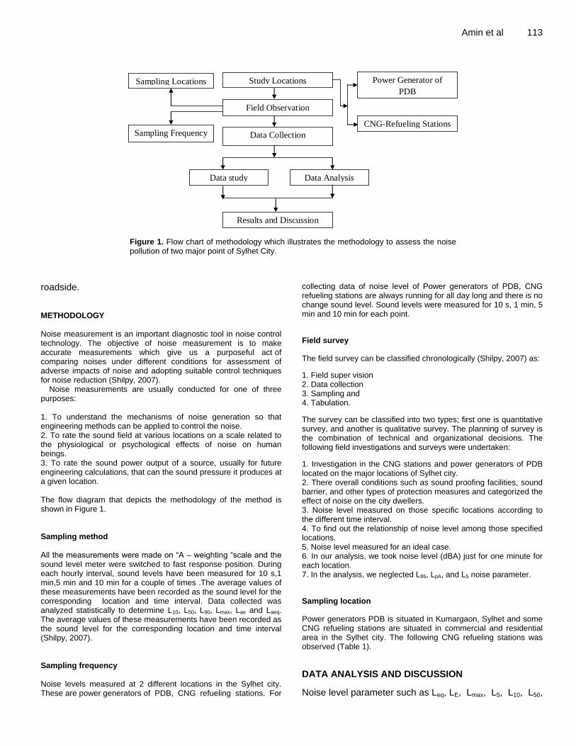
Figure 1. Flow chart of methodology which illustrates the methodology to assess the noise pollution of two major point of Sylhet City.

roadside. METHODOLOGY Noise measurement is an important diagnostic tool in noise control technology. The objective of noise measurement is to make accurate measurements which give us a purposeful act of comparing noises under different conditions for assessment of adverse impacts of noise and adopting suitable control techniques for noise reduction (Shilpy, 2007).

Noise measurements are usually conducted for one of three purposes: 1. To understand the mechanisms of noise generation so that engineering methods can be applied to control the noise. 2. To rate the sound field at various locations on a scale related to the physiological or psychological effects of noise on human beings. 3. To rate the sound power output of a source, usually for future engineering calculations, that can the sound pressure it produces at a given location. The flow diagram that depicts the methodology of the method is shown in Figure 1. Sampling method All the measurements were made on “A – weighting “scale and the sound level meter were switched to fast response position. During each hourly interval, sound levels have been measured for 10 s,1 min,5 min and 10 min for a couple of times .The average values of these measurements have been recorded as the sound level for the corresponding location and time interval. Data collected was analyzed statistically to determine L10, L50, L90, Lmax, Lae and Laeq. The average values of these measurements have been recorded as the sound level for the corresponding location and time interval (Shilpy, 2007). Sampling frequency Noise levels measured at 2 different locations in the Sylhet city. These are power generators of PDB, CNG refueling stations. For

collecting data of noise level of Power generators of PDB, CNG refueling stations are always running for all day long and there is no change sound level. Sound levels were measured for 10 s, 1 min, 5 min and 10 min for each point.

Field survey

The field survey can be classified chronologically (Shilpy, 2007) as:

1. Field super vision 2. Data collection 3. Sampling and 4. Tabulation.

The survey can be classified into two types; first one is quantitative survey, and another is qualitative survey. The planning of survey is the combination of technical and organizational decisions. The following field investigations and surveys were undertaken:

1. Investigation in the CNG stations and power generators of PDB located on the major locations of Sylhet city. 2. There overall conditions such as sound proofing facilities, sound barrier, and other types of protection measures and categorized the effect of noise on the city dwellers. 3. Noise level measured on those specific locations according to the different time interval. 4. To find out the relationship of noise level among those specified locations. 5. Noise level measured for an ideal case. 6. In our analysis, we took noise level (dBA) just for one minute for each location. 7. In the analysis, we neglected L95, LpA, and L5 noise parameter.

Sampling location

Power generators PDB is situated in Kumargaon, Sylhet and some CNG refueling stations are situated in commercial and residential area in the Sylhet city. The following CNG refueling stations was observed (Table 1).

DATA ANALYSIS AND DISCUSSION

Noise level parameter such as Leq, LE, Lmax, L5, L10, L50,


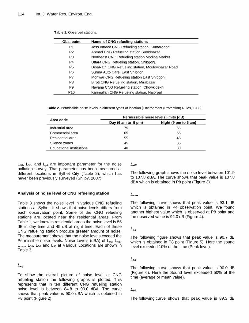
Table 1. Observed stations.

Obs. point Name of CNG-refueling stations

P1 Jess Intraco CNG Refueling station, Kumargaon

P2 Ahmad CNG Refueling station Subidbazar

P3 Northeast CNG Refueling station Modina Market

P4 Uttara CNG Refueling station, Shibgonj.

P5 DibaRatri CNG Refueling station, Moulovibazar Road

P6 Surma Auto Care, East Shibgonj

P7 Monwar CNG Refueling station East Shibgonj

P8 Biroti CNG Refueling station, Mirabazar

P9 Navana CNG Refueling station, Chowkidekhi

P10 Karimullah CNG Refueling station, Naiorpul

Table 2. Permissible noise levels in different types of location [Environment (Protection) Rules, 1986].

Area code Permissible noise levels limits (dB)

Day (6 am to 9 pm) Night (9 pm to 6 am)

Industrial area 75 65

Commercial area 65 55

Residential area 55 45

Silence zones 45 35

Educational institutions 40 30

L90, L95, and LpA are important parameter for the noise pollution survey. That parameter has been measured at different locations in Sylhet City (Table 2), which has never been previously surveyed (Shilpy, 2007).

Analysis of noise level of CNG refueling station

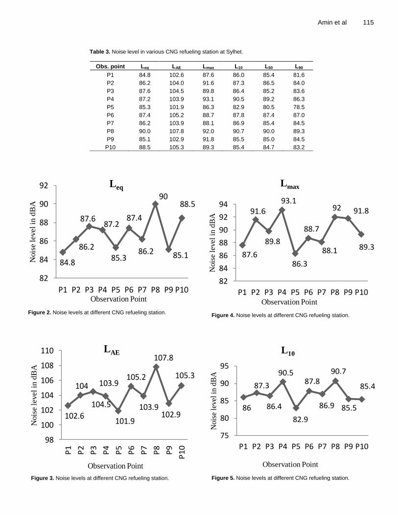
Table 3 shows the noise level in various CNG refueling stations at Sylhet. It shows that noise levels differs from each observation point. Some of the CNG refueling stations are located near the residential areas. From Table 1, we know in residential areas the noise level is 55 dB in day time and 45 dB at night time. Each of these CNG refueling station produce greater amount of noise. The measurement shows that the noise levels exceed the Permissible noise levels. Noise Levels (dBA) of Leq, LAE, Lmax, L10, L50 and L90 at Various Locations are shown in Table 3.

Leq

To show the overall picture of noise level at CNG refueling station the following graphs is plotted. This represents that in ten different CNG refueling station noise level is between 84.8 to 90.0 dBA. The curve shows that peak value is 90.0 dBA which is obtained in P8 point (Figure 2).

LAE

The following graph shows the noise level between 101.9 to 107.8 dBA. The curve shows that peak value is 107.8 dBA which is obtained in P8 point (Figure 3).

Lmax

The following curve shows that peak value is 93.1 dB which is obtained in P4 observation point. We found another highest value which is observed at P8 point and the observed value is 92.0 dB (Figure 4).

L10

The following figure shows that peak value is 90.7 dB which is obtained in P8 point (Figure 5). Here the sound level exceeded 10% of the time (Peak level).

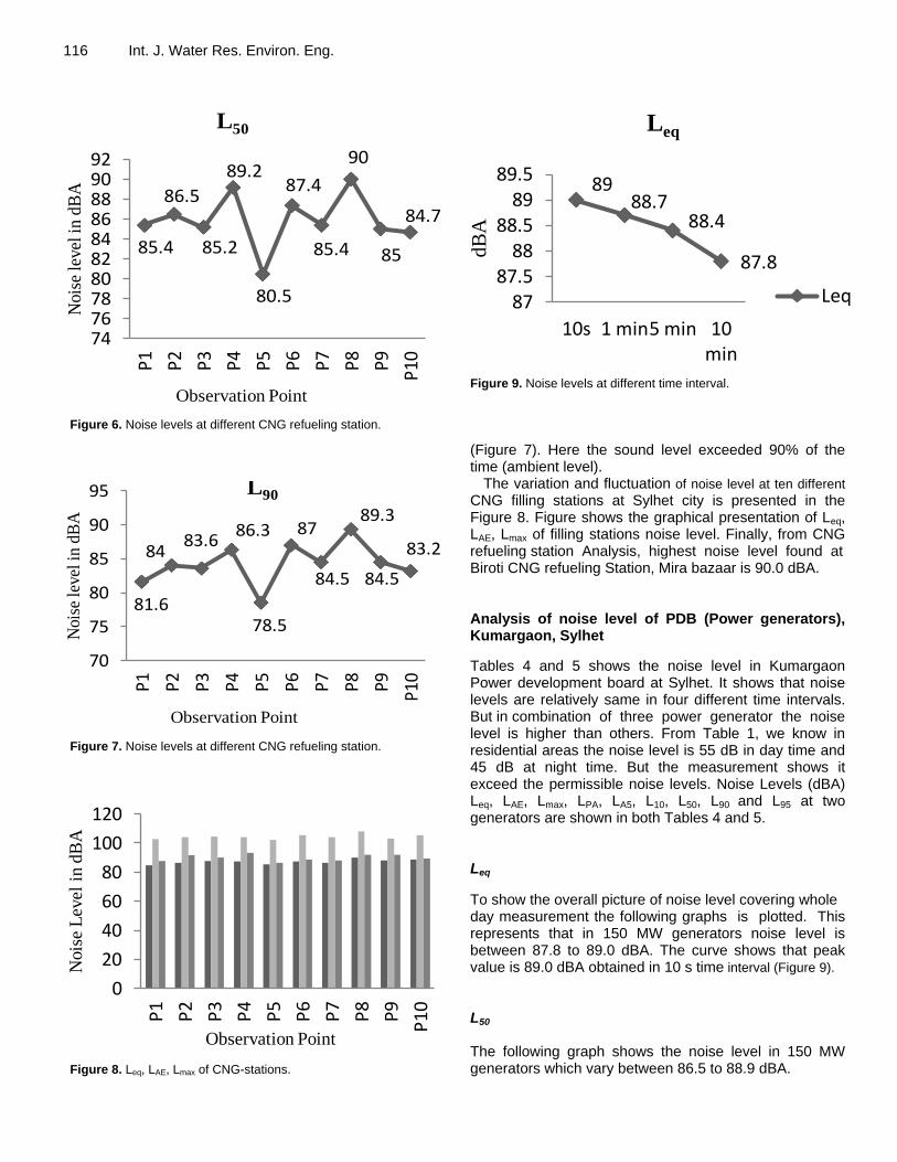
L50

The following curve shows that peak value is 90.0 dB (Figure 6). Here the Sound level exceeded 50% of the time (average or mean value).

L90

The following curve shows that peak value is 89.3 dB

Amin et al 115

Table 3. Noise level in various CNG refueling station at Sylhet.

Obs. point Leq LAE Lmax L10 L50 L90

P1 84.8 102.6 87.6 86.0 85.4 81.6

P2 86.2 104.0 91.6 87.3 86.5 84.0

P3 87.6 104.5 89.8 86.4 85.2 83.6

P4 87.2 103.9 93.1 90.5 89.2 86.3

P5 85.3 101.9 86.3 82.9 80.5 78.5

P6 87.4 105.2 88.7 87.8 87.4 87.0

P7 86.2 103.9 88.1 86.9 85.4 84.5

P8 90.0 107.8 92.0 90.7 90.0 89.3

P9 85.1 102.9 91.8 85.5 85.0 84.5

P10 88.5 105.3 89.3 85.4 84.7 83.2

84.8

86.2

87.687.2

85.3

87.4

86.2

90

85.1

88.5

82

84

86

88

90

92

P1 P2 P3 P4 P5 P6 P7 P8 P9 P10

Nois

e level in

dB

A

Observation PointFig-1.2: Noise levels at different CNG

refueling station.

Leq

Figure 2. Noise levels at different CNG refueling station.

102.6

104

104.5

103.9

101.9

105.2

103.9

107.8

102.9

105.3

98

100

102

104

106

108

110

P1

P2

P3

P4

P5

P6

P7

P8

P9

P1

0

Nois

e level in

dB

A


refueling station.

LAE


87.6

91.6

89.8

93.1

86.3

88.7

88.1

92 91.8

89.3

82

84

86

88

90

92

94

P1 P2 P3 P4 P5 P6 P7 P8 P9 P10

Nois

e le

vel

in

dB

A


refueling station.

Lmax


86

87.3

86.4

90.5

82.9

87.8

86.9

90.7

85.5

85.4

75

80

85

90

95

P1 P2 P3 P4 P5 P6 P7 P8 P9 P10

Nois

e le

vel

in

dB

A


refueling station.

L10



85.4

86.5

85.2

89.2

80.5

87.4

85.4

90

85

84.7

74767880828486889092

P1 P2 P3 P4 P5 P6 P7 P8 P9 P10

Noi

se lev

el in

dB

A

Observation PointFig-1.6:Noise levels at different CNG

refueling station.

L50


81.6

8483.6

86.3

78.5

87

84.5

89.3

84.5

83.2

70

75

80

85

90

95

P1 P2 P3 P4 P5 P6 P7 P8 P9 P10

Noi

se lev

el in d

BA

Observation PointFig-1.7:Noise levels at different CNG

refueling station.

L90


0

20

40

60

80

100

120

P1

P2

P3

P4

P5

P6

P7

P8

P9

P10

Nois

e L

evel

in

dB

A

Observation PointFig- 1.8:Leq, LAE, Lmax of CNG-stations.

Figure 8. Leq, LAE, Lmax of CNG-stations.

8988.7

88.4

87.8

8787.5

8888.5

8989.5

10s 1 min5 min 10 min

dB

A

Fig-1.9: Noise levels at different time

interval.

Leq

Leq

Figure 9. Noise levels at different time interval.

(Figure 7). Here the sound level exceeded 90% of the time (ambient level).

The variation and fluctuation of noise level at ten different

CNG filling stations at Sylhet city is presented in the Figure 8. Figure shows the graphical presentation of Leq, LAE, Lmax of filling stations noise level. Finally, from CNG refueling station Analysis, highest noise level found at Biroti CNG refueling Station, Mira bazaar is 90.0 dBA. Analysis of noise level of PDB (Power generators), Kumargaon, Sylhet

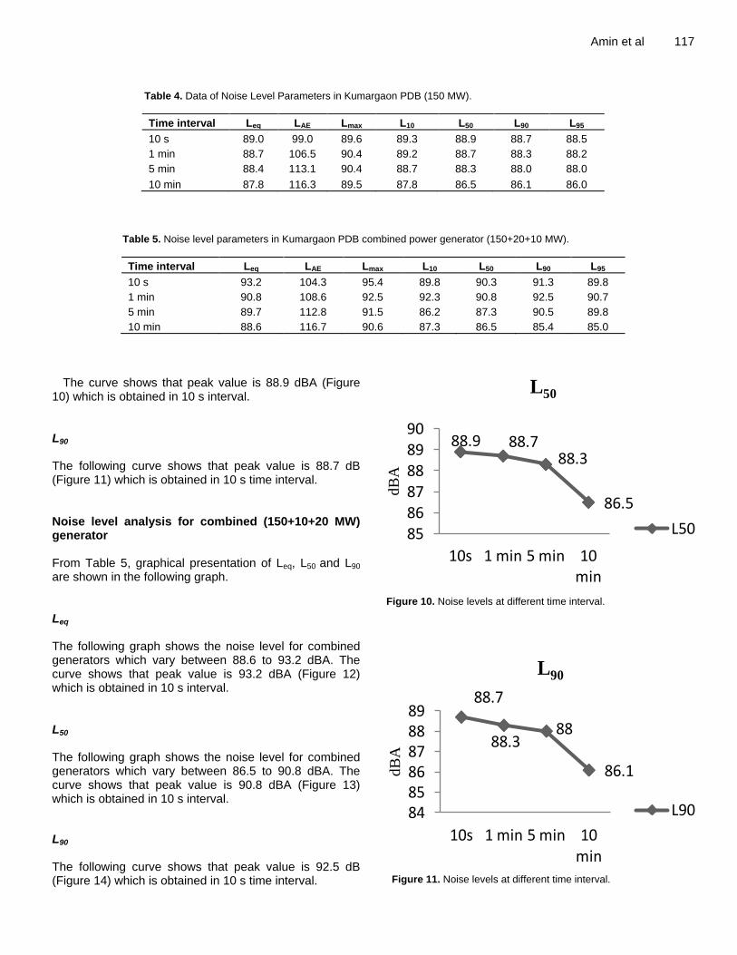
Tables 4 and 5 shows the noise level in Kumargaon Power development board at Sylhet. It shows that noise levels are relatively same in four different time intervals. But in combination of three power generator the noise level is higher than others. From Table 1, we know in residential areas the noise level is 55 dB in day time and 45 dB at night time. But the measurement shows it exceed the permissible noise levels. Noise Levels (dBA) Leq, LAE, Lmax, LPA, LA5, L10, L50, L90 and L95 at two generators are shown in both Tables 4 and 5. Leq

To show the overall picture of noise level covering whole day measurement the following graphs is plotted. This represents that in 150 MW generators noise level is between 87.8 to 89.0 dBA. The curve shows that peak value is 89.0 dBA obtained in 10 s time interval (Figure 9). L50 The following graph shows the noise level in 150 MW generators which vary between 86.5 to 88.9 dBA.

Amin et al 117

Table 4. Data of Noise Level Parameters in Kumargaon PDB (150 MW).

Time interval Leq LAE Lmax L10 L50 L90 L95

10 s 89.0 99.0 89.6 89.3 88.9 88.7 88.5

1 min 88.7 106.5 90.4 89.2 88.7 88.3 88.2

5 min 88.4 113.1 90.4 88.7 88.3 88.0 88.0

10 min 87.8 116.3 89.5 87.8 86.5 86.1 86.0

Table 5. Noise level parameters in Kumargaon PDB combined power generator (150+20+10 MW).

Time interval Leq LAE Lmax L10 L50 L90 L95

10 s 93.2 104.3 95.4 89.8 90.3 91.3 89.8

1 min 90.8 108.6 92.5 92.3 90.8 92.5 90.7

5 min 89.7 112.8 91.5 86.2 87.3 90.5 89.8

10 min 88.6 116.7 90.6 87.3 86.5 85.4 85.0

The curve shows that peak value is 88.9 dBA (Figure 10) which is obtained in 10 s interval. L90

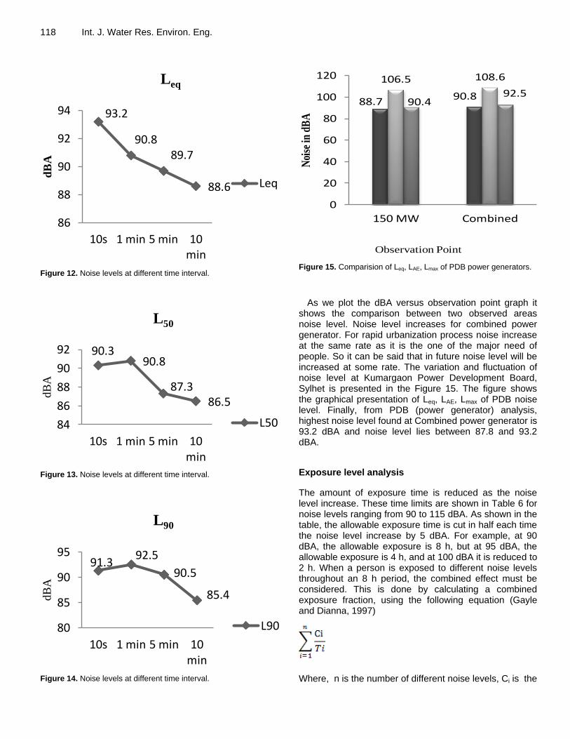
The following curve shows that peak value is 88.7 dB (Figure 11) which is obtained in 10 s time interval. Noise level analysis for combined (150+10+20 MW) generator From Table 5, graphical presentation of Leq, L50 and L90

are shown in the following graph. Leq The following graph shows the noise level for combined generators which vary between 88.6 to 93.2 dBA. The curve shows that peak value is 93.2 dBA (Figure 12) which is obtained in 10 s interval. L50 The following graph shows the noise level for combined generators which vary between 86.5 to 90.8 dBA. The curve shows that peak value is 90.8 dBA (Figure 13) which is obtained in 10 s interval.

L90 The following curve shows that peak value is 92.5 dB (Figure 14) which is obtained in 10 s time interval.

88.9 88.788.3

86.5

858687888990

10s 1 min 5 min 10 min

dB

A


interval.

L50

L50


88.7

88.388

86.1

848586878889


dB

A


interval.

L90

L90



93.2

90.889.7

88.6

86

88

90

92

94


dB

A

Leq

Leq


90.390.8

87.386.5

84

86

88

90

92


dB

A


interval.

L50

L50


91.392.5

90.5

85.4

80

85

90

95


dB

A


interval.

L90

L90


88.790.8

106.5 108.6

90.492.5

0

20

40

60

80

100

120

150 MW Combined

Noi

se in

dB

A

Observation PointFig-1.15: Comparision of Leq, LAE, Lmax of

PDB power generators.

Figure 15. Comparision of Leq, LAE, Lmax of PDB power generators.

As we plot the dBA versus observation point graph it shows the comparison between two observed areas noise level. Noise level increases for combined power generator. For rapid urbanization process noise increase at the same rate as it is the one of the major need of people. So it can be said that in future noise level will be increased at some rate. The variation and fluctuation of noise level at Kumargaon Power Development Board, Sylhet is presented in the Figure 15. The figure shows the graphical presentation of Leq, LAE, Lmax of PDB noise level. Finally, from PDB (power generator) analysis, highest noise level found at Combined power generator is 93.2 dBA and noise level lies between 87.8 and 93.2 dBA.

Exposure level analysis

The amount of exposure time is reduced as the noise level increase. These time limits are shown in Table 6 for noise levels ranging from 90 to 115 dBA. As shown in the table, the allowable exposure time is cut in half each time the noise level increase by 5 dBA. For example, at 90 dBA, the allowable exposure is 8 h, but at 95 dBA, the allowable exposure is 4 h, and at 100 dBA it is reduced to 2 h. When a person is exposed to different noise levels throughout an 8 h period, the combined effect must be considered. This is done by calculating a combined exposure fraction, using the following equation (Gayle and Dianna, 1997)

Where, n is the number of different noise levels, Ci is the

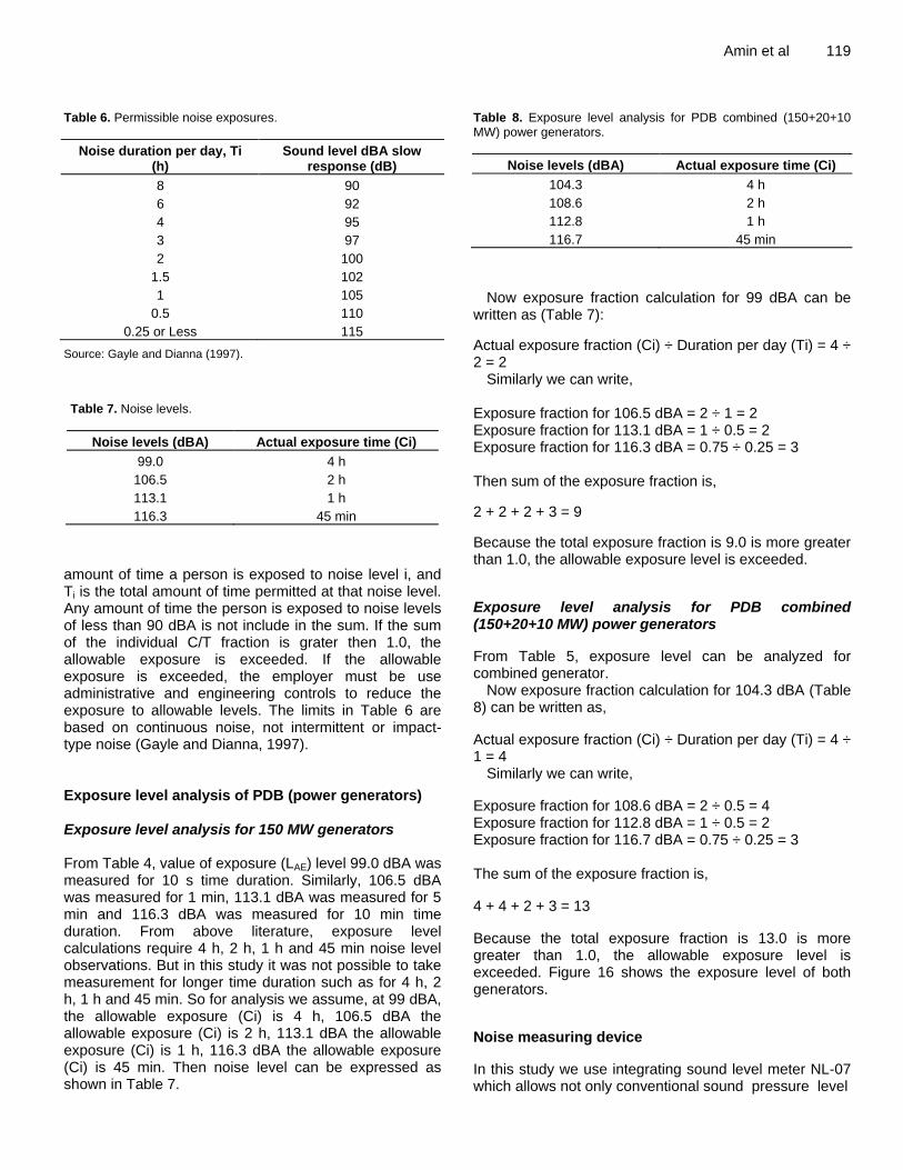
Table 6. Permissible noise exposures.

Noise duration per day, Ti (h)

Sound level dBA slow response (dB)

8 90

6 92

4 95

3 97

2 100

1.5 102

1 105

0.5 110

0.25 or Less 115

Source: Gayle and Dianna (1997).

Table 7. Noise levels.

Noise levels (dBA) Actual exposure time (Ci)

99.0 4 h

106.5 2 h

113.1 1 h

116.3 45 min

amount of time a person is exposed to noise level i, and Ti is the total amount of time permitted at that noise level. Any amount of time the person is exposed to noise levels of less than 90 dBA is not include in the sum. If the sum of the individual C/T fraction is grater then 1.0, the allowable exposure is exceeded. If the allowable exposure is exceeded, the employer must be use administrative and engineering controls to reduce the exposure to allowable levels. The limits in Table 6 are based on continuous noise, not intermittent or impact-type noise (Gayle and Dianna, 1997). Exposure level analysis of PDB (power generators) Exposure level analysis for 150 MW generators From Table 4, value of exposure (LAE) level 99.0 dBA was measured for 10 s time duration. Similarly, 106.5 dBA was measured for 1 min, 113.1 dBA was measured for 5 min and 116.3 dBA was measured for 10 min time duration. From above literature, exposure level calculations require 4 h, 2 h, 1 h and 45 min noise level observations. But in this study it was not possible to take measurement for longer time duration such as for 4 h, 2 h, 1 h and 45 min. So for analysis we assume, at 99 dBA, the allowable exposure (Ci) is 4 h, 106.5 dBA the allowable exposure (Ci) is 2 h, 113.1 dBA the allowable exposure (Ci) is 1 h, 116.3 dBA the allowable exposure (Ci) is 45 min. Then noise level can be expressed as shown in Table 7.

Amin et al 119 Table 8. Exposure level analysis for PDB combined (150+20+10 MW) power generators.

Noise levels (dBA) Actual exposure time (Ci)

104.3 4 h

108.6 2 h

112.8 1 h

116.7 45 min

Now exposure fraction calculation for 99 dBA can be written as (Table 7):

Actual exposure fraction (Ci) ÷ Duration per day (Ti) = 4 ÷ 2 = 2

Similarly we can write, Exposure fraction for 106.5 dBA = 2 ÷ 1 = 2 Exposure fraction for 113.1 dBA = 1 ÷ 0.5 = 2 Exposure fraction for 116.3 dBA = 0.75 ÷ 0.25 = 3 Then sum of the exposure fraction is,

2 + 2 + 2 + 3 = 9

Because the total exposure fraction is 9.0 is more greater than 1.0, the allowable exposure level is exceeded.

Exposure level analysis for PDB combined (150+20+10 MW) power generators

From Table 5, exposure level can be analyzed for combined generator.

Now exposure fraction calculation for 104.3 dBA (Table 8) can be written as,

Actual exposure fraction (Ci) ÷ Duration per day (Ti) = 4 ÷ 1 = 4

Similarly we can write,

Exposure fraction for 108.6 dBA = 2 ÷ 0.5 = 4 Exposure fraction for 112.8 dBA = 1 ÷ 0.5 = 2 Exposure fraction for 116.7 dBA = 0.75 ÷ 0.25 = 3 The sum of the exposure fraction is,

4 + 4 + 2 + 3 = 13

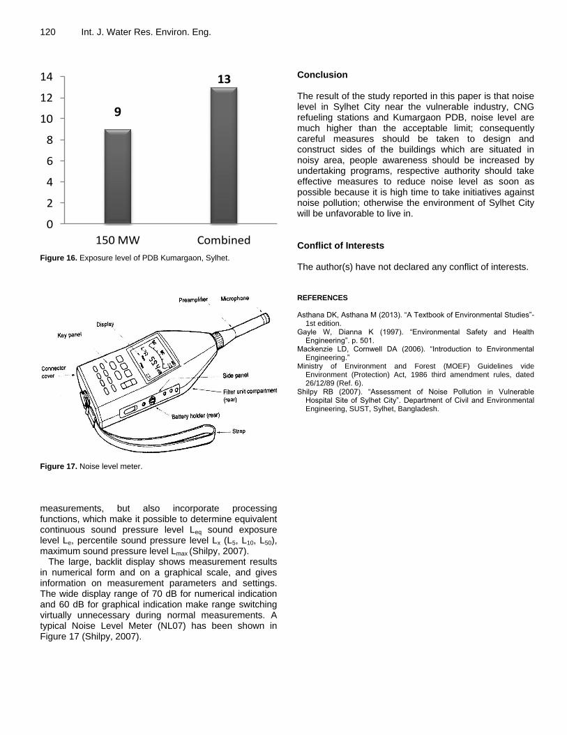
Because the total exposure fraction is 13.0 is more greater than 1.0, the allowable exposure level is exceeded. Figure 16 shows the exposure level of both generators.

Noise measuring device

In this study we use integrating sound level meter NL-07 which allows not only conventional sound pressure level


9

13

0

2

4

6

8

10

12

14

150 MW Combined

Figure 16. Exposure level of PDB Kumargaon, Sylhet.

Fig- 1.17: Noise Level Meter.

Figure 17. Noise level meter.

measurements, but also incorporate processing functions, which make it possible to determine equivalent continuous sound pressure level Leq sound exposure level Le, percentile sound pressure level Lx (L5, L10, L50), maximum sound pressure level Lmax (Shilpy, 2007).

The large, backlit display shows measurement results in numerical form and on a graphical scale, and gives information on measurement parameters and settings. The wide display range of 70 dB for numerical indication and 60 dB for graphical indication make range switching virtually unnecessary during normal measurements. A typical Noise Level Meter (NL07) has been shown in Figure 17 (Shilpy, 2007).

Conclusion The result of the study reported in this paper is that noise level in Sylhet City near the vulnerable industry, CNG refueling stations and Kumargaon PDB, noise level are much higher than the acceptable limit; consequently careful measures should be taken to design and construct sides of the buildings which are situated in noisy area, people awareness should be increased by undertaking programs, respective authority should take effective measures to reduce noise level as soon as possible because it is high time to take initiatives against noise pollution; otherwise the environment of Sylhet City will be unfavorable to live in. Conflict of Interests The author(s) have not declared any conflict of interests. REFERENCES Asthana DK, Asthana M (2013). “A Textbook of Environmental Studies”-

1st edition. Gayle W, Dianna K (1997). “Environmental Safety and Health

Engineering”. p. 501. Mackenzie LD, Cornwell DA (2006). “Introduction to Environmental

Engineering.” Ministry of Environment and Forest (MOEF) Guidelines vide

Environment (Protection) Act, 1986 third amendment rules, dated 26/12/89 (Ref. 6).

Shilpy RB (2007). “Assessment of Noise Pollution in Vulnerable Hospital Site of Sylhet City”. Department of Civil and Environmental Engineering, SUST, Sylhet, Bangladesh.

Documents

Water Resources and - Academic Journals