Wage Gaps and Occupational Segregation

An Analysis of Wage Gaps for Minority Races in the US across States and

Occupations

In this paper we use data from the American Community Survey in the US for 2014 to

analyze the presence of wage and occupational gap for minority races in the US economy.

We tested for wage differences across two dimensions: states and occupations, and attempted

to determine if the difference in wage levels arose due to occupational segregation or if they

could solely be explained by other factors such as education. We found that wage levels for

non-Hispanic whites were consistently higher than all minority races across most states.

However, these gaps are reduced when controlled for occupation. Although whites still have

higher wages, this are explained by the type of job they are doing. Our findings show

evidence of occupational segregation; there is a high proportion of minorities working in in

low paying jobs, and a low proportion in high paying jobs (compared to whites). This is true

for Hispanics and Blacks, but for Asians there is no strong evidence that supports it.

Aishath Zara Nizar

Jose Diaz Barriga Ocampo

Byungchul Yea

Special Project required for the completion of Masters of Arts in Economics

New York University

December 2016

2

I. Introduction

The United States (US) has had a decreasing trend of non-Hispanic whites in its population as

diverse races or ethnicity groups have immigrated into the country. The proportion of non-

Hispanic whites has decreased from 76% in 1990 to 65% in 2010 (U.S Census Bureau),

which has had a large impact on the labor dynamics in the US. As more people of color

immigrate into the country, there have been specific trends observed about the type of jobs a

particular ethnic or racial group are more inclined towards, determined by a considerable

number of factors such as geography, immigration status (legal or not), ability and fluency in

speaking English and education. Moreover, a large amount of research has recognized that

minority groups have faced consistent wage discrimination in the labor market even up until

today. Thus, we recognize the pivotal interplay between wage differences and occupational

segregation of minority races in the US.

Many studies have documented the relationship between wages, race, education, gender and

occupation. Some of them, such as Catanzarite (2000), show that occupational segregation

exists at local levels such as metropolitan areas or selected cities. Also, Farley (1989, 1990)

investigated economic performance based upon racial identification. He found that virtually

all of the racially self-declared white minorities have economic profiles at or above the

national mean and all of them had higher per capita incomes than black.

However, as far as we know, there has been no study that has analyzed wage differences in

the US at the state and occupation levels. We use data from the Integrated Public Use

Microdata Series (IPUMS), which includes raw data originally collected from the American

Community Survey, for 2014, with a final sample of more than one million observations. We

essentially build upon Becker’s (1957) framework as a theoretical model, which is given by:

3

where Y is an (n x 1) vector of observed wages, X is an (n x k) vector of exogenous

explanatory variables and Z is an (n x j) vector indicating membership in a minority group.

Our research aims to compare the interaction between wage and race in all racial groups

against non-Hispanic whites using recent data by considering state and occupations.

Furthermore, we want to see if there is evidence of wage discrimination across races, and

how much of that can be explained through state-specific and occupation-specific

characteristics. We also believe that there may exist occupational segregation within races,

which may help to explain these differences in wages. We further delve into possible wage

differences within occupations, which may give stronger evidence of wage discrimination

(after controlling for basic wage determinants as education, age and gender).

Our paper is structured as follows: Section 2 lays out the literature review which we based

our research on while Section 3 summarizes the data used in our analysis. Section 4 explains

in detail our basic model; and discusses the regression results in which we attempt to

compare wage gaps across states and occupations, determine factors which may explain the

magnitude of these gaps, and link these results to the extent of occupational segregation we

find in our data. We conclude with a brief look at the limitations in our analysis and avenues

for future research.

4

II. Literature Review

The primary paper we based our research on is a study by Carlos Gradin at el. (2011) titled

“Occupational Segregation by Race and Ethnicity in the US: Differences across States”. This

paper analyzed occupational segregation in the US, conditional and non-conditional at the

state level. The empirical model uses cross sectional data from 2005 to 2007 from the Public

Use Microdata Samples (PUMS) files of the American Community Survey.

The unconditional analysis showed that District of Columbia, New Jersey, Hawaii, and

Southwestern states have a high degree of segregation by race and ethnicity. It hypothesized

that the main reasons for this disparity are an uneven distribution of workers and a diversity

in industrial structures across states. The key result is that the wage segregation is

significantly reduced after conditioning by racial composition in the states (controlling for

races). Moreover, the states with the biggest negative gap were the ones located in the East

Central region such as Kentucky, Alabama, Tennessee, and Indiana.

The second paper is titled “Workplace Segregation in the United States: Race, Ethnicity, and

Skill” (Judith K. Hellerstein and David Neumark, 2008). This paper studies measurements of

workplace segregation by education, language, race, and ethnicity in the US and skill

differences based on race and ethnic segregation. It uses Decennial Employer-Employee

Database for 1990, using a Monte Carlo simulation for random occurring segregation.

The analysis was based on the percentage of workers in an individual’s establishment or

workplace in different demographic groups that average the percentages separately for each

group in the sample. The primary result is that the differences in wages can be explained by

education and skills for white workers (17%), but for Hispanic workers, language is more

significant in explaining the wage gap (29%). Additionally, the magnitude explained by each

5

race is almost the same size as the one explained by education (14%), Hispanic having the

biggest negative impact (20%). This paper gives a good insight into the idea that education,

skill, and race affects workplace segregation.

The third paper is entitled “Explaining Differences in Economic Performance Among Racial

and Ethnic Groups in the USA: The Data Examined” (William Darity Jr. et al, 1996). The

authors begin by measuring the effects of races in wages in both men and women. Later, they

introduce control variables such as English fluency, foreign or domestic site of birth, and

indicator of the extent to which a person is assimilated. The conclusion was that there is no

systemic evidence of discriminatory differentials affecting the income between ethnic groups

on women. Japanese, Chinese, and Korean men show strong evidence of a flip from negative

to positive gap on their behalf. This paper provides a basic guideline for thinking about the

necessary factors to control for race as well as gender.

III. Data

The data used in our study is from the IPUMS database. We used annual data for 2014

throughout the study, for our analysis to reflect the most recent data available. Table 1 below

summarizes the variables used.

In all our analyses, the dependent variable is the natural log of wage. Our main variable of

interest is race; in the original IPUMS dataset, only the following five races are explicitly

recorded as dummy variables for race: white, Black, Asian, Pacific Islander, and American

Indian or Alaska Native. We combined the last two variables (Pacific Islander, American

Indian or Alaska Native) due to the small number of observations in each.

6

Table 1: Data details

Variable Type Description Values

wage continuous Each individual’s total pre-tax wage and

salary income from an employer;

measured in current U.S. dollars

Ranges from 10,000 to

642,000

age Factor with

14 levels Individual’s age, grouped by 5-year

terms1

16-20 years, 21-25 years, ….

76-80 years, 81-100 years

education Factor with 4

levels Level of education, transformed to a

factor variable based on the years of

education of each individual

Less than high school, high

school, incomplete college,

college or more

sex Factor with 2

levels Gender of the individual Male, female

race Factor with 6

levels Race of the individual White, Black, Hispanic,

Asian, Pacific Islander and

Native American, Mixed

race

state Factor with

51 levels State where the individual lives All 50 states and District of

Columbia

minor_ occupation

Factor with

97 levels Occupation of each individual based on

the 2010 Standard Occupational

Classification (SOC)’s minor occupation

groups

major_ occupation

Factor with

23 levels Occupation of each individual based on

the 2010 SOC’s major occupation groups

Hispanic (as a variable), is recorded separately (since it is an ethnicity and not a race),

classing people according to their country of origin.2 We manipulated this variable to also

follow a dummy variable classification with 1 being Hispanic and 0 being not Hispanic.

Naturally, there was an overlap between people who identified themselves as Hispanic and of

a particular race. Hence, we further coded the new Hispanic variable such that, if a person is

Hispanic and of another single race, he will be coded as a Hispanic. If a person is Hispanic

and of two or more races, or any other two race combination, we created a new variable,

1 Due to a very small number of observations after 80 years, we made a 20-year term (81-100) as the last age

group. 2 In the IPUMS database, “Hispanics” identifies persons of Hispanic/Spanish/Latino origin where “origin” is

defined by the Census Bureau as ancestry, lineage, heritage, nationality group, or country of birth. This variable

has factors: not Hispanic; Mexican; Puerto Rican; Cuban; other; and not reported.

7

“mixed race”, to account for this. Finally, we combined all these variables to create the “race”

variable, with each race and Hispanic, being a level of this factor variable, where any single

person is only identified as one race or ethnicity..

The minor_occupation and major_occupation variables were created using the occupation

classification code for each individual in the dataset. This is a 6-digit code classifying the

person’s primary occupation, based on the 2010 Standard Occupation Classification system.

Of this 6-digit code, the first two digits represent the major occupation group while the third

digit (along with the first two) represents the minor occupation group.3 We used this

information to create each person’s minor and major occupation groups.

We cleaned the data by removing all individuals who were unemployed or did not specify

their jobs. We also removed individuals who reported less than $10,000 as their yearly

income, which can be attributed to being employed only for a short time during the year. Our

final dataset consisted of 1.2 million observations.

3 For instance, if a person’s 6-digit code was 29-1062 (“Family and General Practitioner”), his major occupation

code would be 29-000 (“Healthcare Practitioners and Technical Occupations”) and his minor occupation code

would be 29-1000 (“Health Diagnosing and Treating Practitioners”).

8

IV. Model and Estimation Method

We used the OLS model to run the regressions for this paper. Using log of wages as the

dependent variable, we controlled for sociodemographic factors in our dataset to determine

the effect of race on wages.

∑

(1)

where i refers to each individual and X is a matrix including the constant and basic

sociodemographic controls (age, gender and education). After this step, we test this equation

by controlling for the state that the individual resides in.

∑

∑

(2)

Alternatively, we added occupation controls to Equation 1. We did so by adding controls in

two variations: major and minor occupations.4 Major occupations consist of 23 levels of

occupation; these are further broadened into 97 levels to make up minor occupation levels.

∑

∑

(3)

∑

∑

(4)

We further enhanced the model by adding both state and occupation controls. This

strengthens our overall evaluation by enabling us to see wage gaps across two dimensions:

states and occupations. The results for all the equations are shown below in Table 2.

4 As explained in Section 3: Data, we followed the 2010 Standard Occupational Classification (SOC) published

and made available by the Bureau of Labor Statistics. Please refer to the appendix or to http://www.bls.gov/soc/

for more details on the occupation levels.

9

∑

∑

∑

(5)

∑

∑

∑

(6)

Table 2: Wage gap of each race relative to non-Hispanic whites, pooled

Hispanic

Black

Asian

Native American

/ Pacific Islander Mixed race

(1) Basic controls -0.1287 ***

-0.1539 ***

-0.0067 **

-0.1401 ***

-0.0543 ***

(2) State controls -0.1811 ***

-0.1711 ***

-0.0664 ***

-0.1422 ***

-0.0827 ***

(3) Major occupations -0.0864 ***

-0.1092 ***

-0.0203 ***

-0.0999 ***

-0.0421 ***

(4) Minor occupations -0.0679 ***

-0.0816 ***

-0.0043 .

-0.0844 ***

-0.0318 ***

(5) State and major

occupations -0.1329 ***

-0.1215 ***

-0.0773 ***

-0.1033 ***

-0.0691 ***

(6) State and minor

occupations -0.1117 ***

-0.0920 ***

-0.0611 ***

-0.0863 ***

-0.0581 ***

*** p-value <0.001, ** p-value <0.01, “.” p-value <0.1

10

Table 2 reports the wage gap estimates for the reference category (males of age 16-20 years

who have not completed high school). Each estimate represents the wage gap of that

particular race against non-Hispanic whites. The negative sign of all coefficients that hold

throughout imply that all minority groups receive lower wages than their non-Hispanic white

counterparts. It can be observed that as we add more stringent occupation controls, the

regression coefficients, with the exception of Asians, are all becoming smaller in absolute

terms, while still remaining significant (i.e. the wage gap is becoming smaller as we move

from Equation 1, to 3 and 4). This implies that specifying more details about the type of job

helps to explain the wage gaps between races.

After adjusting for the minor group of occupations (Equation 4), we see that Native

Americans and Pacific Islanders, and Blacks have the largest wage gap, receiving 8.4% and

8.2%, less than whites for the reference category, respectively. Asians have the smallest wage

gap, and further, shows the smallest reduction in the wage gap after adding the occupation

controls.

It is also interesting to note from the results above, that adding state controls cause the

regression coefficients to become larger (by moving in the opposite direction than what we

expected). The estimates from Equation (2), (5) and (6) indicate that specifying each

individual’s state causes the wage gap to become larger, possibly pointing to the fact that

there is a bigger concentration of minorities (particularly Hispanics and Blacks) in poorer

states.

Looking at the other control variables, we noted that the estimates for the gender variable (a

dummy which took 1 for female) was consistently negative throughout; the gender wage gap

11

as per our analysis ranged from -11% to -36% (after controlling for minor occupations)5 with

the smallest wage gap observed in D.C. As for education, the returns on schooling was

positive at all levels and for all states, as expected, with individuals having completed 4 years

of college or more recording the highest level of wages. After controlling for minor

occupations, the highest “college effect” was observed for California and New York.

How do wage gaps compare across states?

To further explore the details of the wage gaps, we then ran Equations (1) and (4) for each of

the 51 states (including D.C.) separately. This enabled us to find out which state had the

largest (and smallest) gaps for each race, and observe the significance for the wage gaps for

each race in specific states. By adding in the occupation controls,6 we were able to tease out

the “occupation” effects in each state. Figure 1 below shows us the wage differences across

states for each race group.

5 The values represent the reference category (a female of 16-20 years who did not complete high school).

6 In this section, all “occupation controls” refer to controlling for the minor level of occupations (and not the

major level of occupations) even though it is not explicitly mentioned.

12

Figure 1: Wage differences by state, without controlling for occupation

Figure 1 shows the results of Equation 1 run separately for each state, obtaining wage gaps for each race, across all states.

These wage gaps are graphed at the same scale across all five maps, where blue colors indicate a negative wage gap ( non-

Hispanic whites have a higher wage than the particular race in that state) and red colors indicate a positive wage gap (the

particular race receive higher wages than non-Hispanic whites in that state). White indicates zero i.e. the wage gap between

the reference group and the minority race is essentially zero. Alaska and Hawaii are only omitted in the graphical

representation. Estimates for all states can be found in the appendix.

In the figure above, the blue colors indicate that non-Hispanic whites have a higher wage than

the given race; red colors illustrate the opposite, that the specific race has an average wage

higher than non-Hispanic whites within the state. The way the scale is constructed makes

these maps comparable with each other. For instance, the biggest difference in wages across

all races is for Blacks in North Dakota. It is clear that non-Hispanic whites have better wages

across all states and across all races. When we control for occupations, the results are as

follows, shown in Figure 2.

13

Figure 2: Wage differences by state, including controls for occupation

Figure 2 shows the results of Equation 4 run separately for each state, obtaining wage gaps for each race

across all states, controlling for the minor level of occupations. These graphs have been constructed at the same

scale as in Figure 1, which means that the magnitude of the gaps (as per the shade of red and blue) in each state

can be compared with all the maps in Figure 2 as well as those in Figure 1. Similar to Figure 1, Alaska and

Hawaii are only omitted in the graphical representation. Estimates for all states can be found in the appendix.

After controlling for occupations we observe some interesting results. In general, the wage

differences are smaller or remain about the same, as we saw for the results in Table 2. States

that have big wage differences still have those differences after controlling for occupation,

although at a smaller scale. This can be seen with the lighter colors in the maps after

controlling for occupation.

There are few states that change color between the two sets of maps; the change in colors

mean that before controlling for occupation there was a positive or negative wage difference,

14

and that it changed when controlling for occupation. For instance, in Oregon, Kansas and

West Virginia, Blacks received lower wages than their non-Hispanic white counterparts

before controlling for occupation. After adding in these controls, theses states became

“red”— Blacks are shown to have a higher wage level than the reference group. This tells us

that the wage gap between whites and Blacks in these states is mainly because of the type of

job they are involved in.

An example of the opposite scenario is given by New Hampshire in the Hispanics graph.

Before controlling for occupation, it is seen that Hispanics receive a higher wage than whites.

After controlling for occupation however, the gap becomes negative, i.e. Hispanics receive a

lower wage than whites within the state. This may point to wage discrimination for Hispanics

in New Hampshire, although the population of Hispanics in New Hampshire may not be big

enough for the results to be interesting.

States that have a big mixture of races such as California, Florida and New York remain

about the same relative to other states, although after controlling for occupations the scale

(and therefore the wage differences) is smaller. Even when wage gaps are reduced after

controlling for occupation, relative to the gaps in other states, the difference remains about

the same. Hispanics, Blacks and Asians have almost the same wage difference in these states.

How do wage gaps compare across occupations?

To obtain a more in-depth picture on the wage gaps, we then proceeded to figure out how

these wage differences fared when compared by occupation. While forgoing the use of “state

controls” since it caused wage gaps to diverge rather than converge, we ran Equation (1) on

two sets of data: on each of the 23 major occupations separately, and on each of the 97 minor

occupations separately. Similar to the “state wage gap” analysis done previously, we were

15

then able to compare how the wage gaps persisted based on the type of the occupation. For

our analysis, we limited ourselves to the results for the major occupations set rather than the

minor occupations (although they provided more reliable estimates in the pooled equations)

due to reduced sample size.7

We show the wage gap by major occupations for Hispanics, Blacks and Asians, ordered by

average wage, below in Figure 3. One of the trends that stand out most in the graph is that

while the wage gap for Hispanics and Blacks are relatively equal, the wage gap for Asians

follows a markedly different course, particularly for higher-paid occupations. Moreover, we

see that Asians receive a higher wage than non-Hispanic whites for higher-paid occupations

(average wage greater than $58,000). Among these three races, the largest positive gap is for

Asians, who receive 15% more than the reference group, in “Healthcare Practitioners and

Technical Occupations”. The trend in where Asians are better paid than most other races can

be attributed to a higher concentration of Asians in these jobs, as well as a larger portion of

Asians being well-educated. The largest negative wage difference is for Hispanics in

“Farming, Fishing, and Forestry Occupations”, receiving almost 25% less on average than

non-Hispanic whites.

7 This was because once the equation was run for each 97 occupation separately, some races had a handful of

people in some occupations, leading to substantially biased estimates. For instance, only two Asians, five Native

American and Pacific Islanders and five persons of mixed race worked in the occupation “Helpers, construction

trades”.

16

Figure 3: Wage differences by occupation

What drives state and occupation gaps?

From the state-level and occupation-level wage differences we found in our earlier analyses,

we then proceeded to find out whether the level of the wage gaps across states could be

explained by certain characteristics of the state, and whether the level of the wage differences

by occupation could be explained by similar job-specific explanatory variables. To test the

state gaps, we used the coefficients obtained from Equation 4 (run separately for each state)

to be the dependent variables and tested for the following:

a. Do wage gaps across states differ based on geographic regions?

b. Do richer states have higher wage gaps between races?

c. Are wage gaps lower in states where minorities are a larger fraction of the population?

-0.30

-0.20

-0.10

0.00

0.10

0.20Fo

od

Pre

par

atio

n a

nd

Ser

vin

g R

elat

ed O

ccu

pat

ion

s

Per

son

al C

are

and

Ser

vice

Occ

up

atio

ns

Hea

lth

care

Su

pp

ort

Occ

up

atio

ns

Bu

ildin

g an

d G

rou

nd

s C

lean

ing

and

Mai

nte

nan

ce…

Farm

ing,

Fis

hin

g, a

nd

Fo

rest

ry O

ccu

pat

ion

s

Off

ice

and

Ad

min

istr

ativ

e Su

pp

ort

Occ

up

atio

ns

Tran

spo

rtat

ion

an

d M

ater

ial M

ovi

ng

Occ

up

atio

ns

Pro

du

ctio

n O

ccu

pat

ion

s

Co

mm

un

ity

and

So

cial

Ser

vice

Occ

up

atio

ns

Mili

tary

Sp

ecif

ic O

ccu

pat

ion

s

Co

nst

ruct

ion

an

d E

xtra

ctio

n O

ccu

pat

ion

s

Edu

cati

on

, Tra

inin

g, a

nd

Lib

rary

Occ

up

atio

ns

Inst

alla

tio

n, M

ain

ten

ance

, an

d R

epai

r O

ccu

pat

ion

s

Pro

tect

ive

Serv

ice

Occ

up

atio

ns

Sale

s an

d R

elat

ed O

ccu

pat

ion

s

Art

s, D

esig

n, E

nte

rtai

nm

ent,

Sp

ort

s, a

nd

Me

dia

…

Life

, Ph

ysic

al, a

nd

So

cial

Sci

ence

Occ

up

atio

ns

Bu

sin

ess

and

Fin

anci

al O

per

atio

ns

Occ

up

atio

ns

Hea

lth

care

Pra

ctit

ion

ers

an

d T

ech

nic

al O

ccu

pat

ion

s

Arc

hit

ectu

re a

nd

En

gin

eeri

ng

Occ

up

atio

ns

Co

mp

ute

r an

d M

ath

emat

ical

Occ

up

atio

ns

Man

agem

ent

Occ

up

atio

ns

Lega

l Occ

up

atio

ns

Hispanic

Black

Asian

In Figure 3, the x-axis shows all

the 23 major occupation

groups, arranged in ascending

order based on the average

way. The left-most occupation is

Food Preparation and Serving

Related Occupations, with an

average wage of about $22,500

and the highest-paid occupation

is Legal Occupations, with an

average wage of about

$117,000. It is important to note

that, although the occupations

on the x-axis are placed equally

apart, the average wage gap

between any two occupations is

not uniform. The curves show

the wage gap for each of the

three major races, for each

occupation separately

17

It is not obvious from the state maps, but we wanted to test whether the wage gaps were

statistically different in the different regions. For instance, do minority races receive higher or

lower wages compared to whites, based on which geographic region they live in? We

hypothesize that the wage gap may be more different in southern and midwestern and

northeastern states, perhaps due to the differences in work culture and industries.

We also hypothesize that for richer states, which potentially have more competitive job

markets, the wage differences between races may be smaller compared to poorer and more

rural states, where wage discrimination can be more ingrained. As for the third conjecture, we

believe that there could be a “diversity effect” — in states with a higher share of minorities,

there is a more level playing field in the job market due to a greater participation in the

workforce by non-white races, therefore leading to lower wage gaps between races. For

example, for Hispanic men in California the average share of co-workers who are Hispanic is

51.1%, whereas in Florida it is over 6 percent points higher, at 57.5% (Judith Hellerstein et.

al, 42). The results of these hypotheses are shown in Table 3, where each row represents a

tested hypothesis.

Table 3: Hypothesis testing for state gaps

Hispanic Black Asian Native American /

Pacific Islander Mixed race

(1) By geography - Northeast

- South

- West

-0.0089 -0.0306 * -0.0285 .

0.0619 0.0146 0.0484

-0.0236 -0.0080 -0.0199

0.1248 *** 0.0373 0.0058

-0.0186 0.0126 0.435 .

(2) By income

- log (GDP per

capita)

-0.0320

-0.0894 .

-0.0739 .

-0.0292

0.0482

(3) By minority

concentration

- 80% white

0.0297 **

0.0249

0.0404 .

0.0162

-0.0413 *

*** p-value <0.001, ** p-value <0.01, * p-value <0.05, “.” p-value <0.1

18

By geography: when testing for geographic regions, we followed the geographical

classification used by the US Census Bureau which adopts a system of four specific regions:

northeast, midwest, south and west. We ran the regression using each region as a dummy

variable and the midwest to be the reference category. It is interesting that the coefficient

estimates for Hispanics and Asian is negative (although for Asians, the values are not

significant). These imply that for Hispanics, the wage gap is significantly wider in the

southern and western states compared to the midwest. This could be due to a combination of

the concentration of Hispanics in these areas (or the lack of) and the types of jobs with a large

(or small) Hispanic population in these specific states. For Blacks, the estimates suggest the

highest wage gap to be in the midwest itself, with all other regions having lower wage gaps,

but these values are not significant.

By income: the explanatory variable is taken to be the log of the GDP per capita in each state

in 2014. For all races except for the mixed race category, it can be seen that the wage gap is

larger in richer states. This could possibly be due to more competitive labor markets in these

states, or the difference in concentration of minority races in richer states, specifically in

states such as North Dakota and Alaska, whose economy are dominated by few industries.

However, the wage gap is only significant for Blacks and Asians.

By minority concentration: to create a dichotomous variable indicating states of a high level

of minorities, we looked at the median percent of whites in each state (80% in the sample)

and created “low white” cities and “high white” cities (latter being equal to 1). It is

interesting that almost all the coefficients are positive, contrary to our expectation of a

“diversity effect”. Indeed, our results show that racial integration possibly has no effect or a

negative effect on the magnitude of state-level wage gaps. The coefficient estimates are

19

significant for Hispanics and Asians, indicating that the wage gap is smaller for these races in

states where 80% or more of the population is white.

The rationale for testing occupation gaps, was in effect, trying to find out how much of a

wage gap there exists within each occupation— and in what kind of occupations these are the

largest and the smallest. We attempted to find out whether these occupation gaps could be

explained by occupation characteristics. Naturally, there were fewer possible explanatory

variables that we could come up with to explain occupation gaps. We looked at the average

wage of each occupation, dividing the jobs into three categories based on its wage tercile, and

regressed the occupation gaps on these categorical variables.8

Table 4: Hypothesis testing for occupation gaps

Hispanic Black Asian Native American

/ Pacific Islander Mixed race

(1) By wage level of

occupation

- Quartile 2 - Quartile 3

-0.0226 -0.0568***

-0.0394 -0.1003***

-0.0264 -0.0612

-0.0243 -0.1375***

-0.0024 -0.0051

*** p-value <0.001, ** p-value <0.01, * p-value <0.05, “.” p-value <0.1

We find that for occupations that are paid higher, the wage gaps for minority races become

even bigger (as indicated by the negative signs on all the coefficients shown in Table 4).

Interestingly, these effects are significant only on the most highly paid jobs, and are not

observed for the occupations that are in the middle tercile. Further, our regressions show that

such wage gaps by income is not faced by Asians at all. Collectively, this could suggest that

minority races are not able to participate in higher paid jobs as much as whites, essentially,

8 Although earlier in Section 4, we used major occupations to graphically compare occupation gaps, we used the

coefficients obtained from running Equation (1) on each of the minor ooccupations separately in this hypothesis

testing stage. The reason for this was, using minor occupation gaps gave us 97 observations while using major

occupations gave us 23. This meant that the estimates from using only 23 observations would were likely to be

substantially biased due to the small sample size.

20

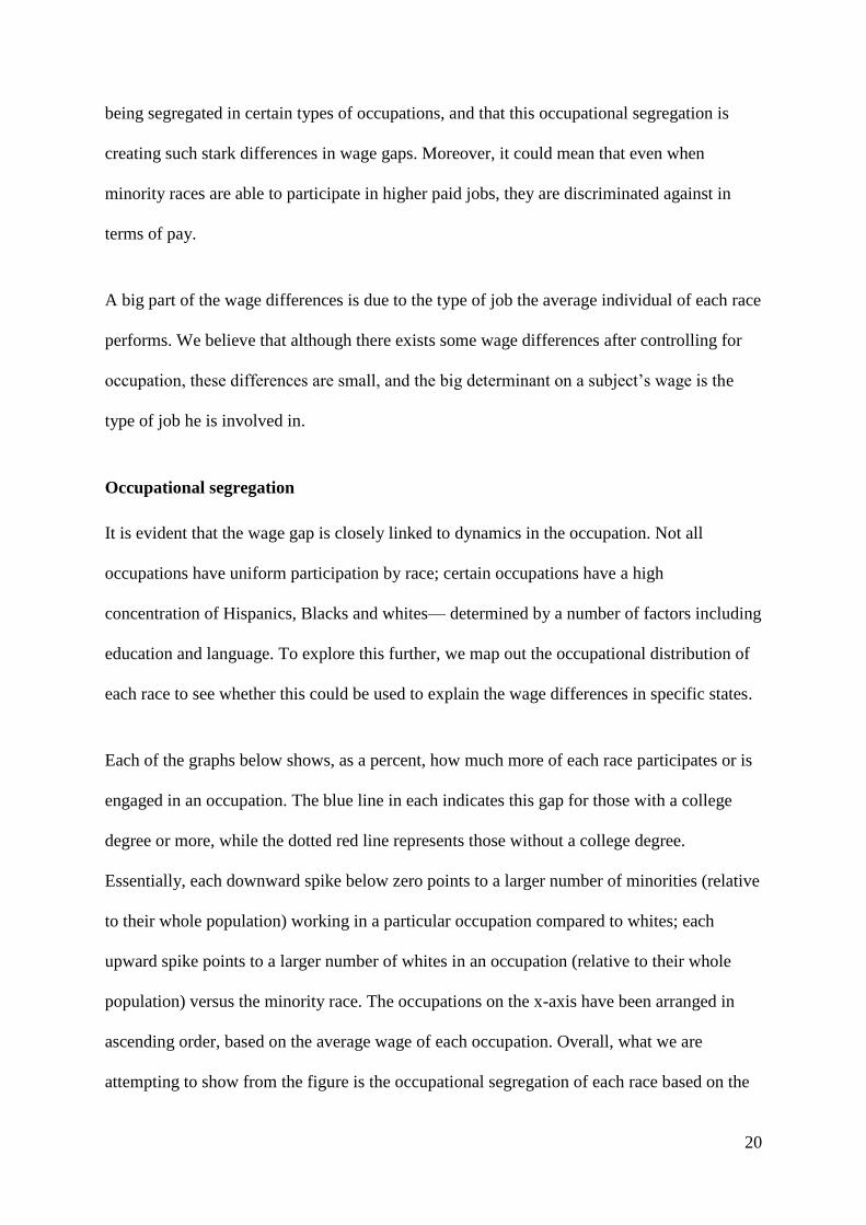
being segregated in certain types of occupations, and that this occupational segregation is

creating such stark differences in wage gaps. Moreover, it could mean that even when

minority races are able to participate in higher paid jobs, they are discriminated against in

terms of pay.

A big part of the wage differences is due to the type of job the average individual of each race

performs. We believe that although there exists some wage differences after controlling for

occupation, these differences are small, and the big determinant on a subject’s wage is the

type of job he is involved in.

Occupational segregation

It is evident that the wage gap is closely linked to dynamics in the occupation. Not all

occupations have uniform participation by race; certain occupations have a high

concentration of Hispanics, Blacks and whites— determined by a number of factors including

education and language. To explore this further, we map out the occupational distribution of

each race to see whether this could be used to explain the wage differences in specific states.

Each of the graphs below shows, as a percent, how much more of each race participates or is

engaged in an occupation. The blue line in each indicates this gap for those with a college

degree or more, while the dotted red line represents those without a college degree.

Essentially, each downward spike below zero points to a larger number of minorities (relative

to their whole population) working in a particular occupation compared to whites; each

upward spike points to a larger number of whites in an occupation (relative to their whole

population) versus the minority race. The occupations on the x-axis have been arranged in

ascending order, based on the average wage of each occupation. Overall, what we are

attempting to show from the figure is the occupational segregation of each race based on the

21

average wage of each. We did not include the graphs for Native American and Pacific

Islanders, and mixed races, as they did not reveal any significant findings.

Figure 3: Occupation segregation gap of each race

-4

-3

-2

-1

0

1

2

3

Oth

er F

oo

d P

rep

arat

ion

an

d S

ervi

ng…

Text

ile, A

pp

arel

, an

d F

urn

ish

ings

Wo

rker

s

Gro

un

ds

Mai

nte

nan

ce W

ork

ers

Foo

d P

roce

ssin

g W

ork

ers

Mat

eria

l Mo

vin

g W

ork

ers

Fore

st, C

on

serv

atio

n, a

nd

Lo

ggin

g W

ork

ers

Pri

nti

ng

Wo

rker

s

Mili

tary

En

liste

d T

acti

cal O

per

atio

ns

and

…

Rel

igio

us

Wo

rker

s

Co

un

selo

rs, S

oci

al W

ork

ers,

an

d O

ther

…

Pre

sch

oo

l, P

rim

ary,

Sec

on

dar

y, a

nd

…

Fun

eral

Ser

vice

Wo

rker

s

Art

an

d D

esig

n W

ork

ers

Firs

t-Li

ne

Enlis

ted

Mili

tary

Su

per

viso

rs

Po

stse

con

dar

y Te

ach

ers

Sup

ervi

sors

of

Co

nst

ruct

ion

an

d…

Soci

al S

cien

tist

s an

d R

elat

ed W

ork

ers

Oth

er M

anag

emen

t O

ccu

pat

ion

s

Mat

hem

atic

al S

cien

ce O

ccu

pat

ion

s

Top

Exe

cuti

ves

Hispanics

With BA Without BA

-4

-3

-2

-1

0

1

2

3

Oth

er F

oo

d P

rep

arat

ion

an

d S

ervi

ng…

Text

ile, A

pp

arel

, an

d F

urn

ish

ings

Wo

rker

s

Gro

un

ds

Mai

nte

nan

ce W

ork

ers

Foo

d P

roce

ssin

g W

ork

ers

Mat

eria

l Mo

vin

g W

ork

ers

Fore

st, C

on

serv

atio

n, a

nd

Lo

ggin

g W

ork

ers

Pri

nti

ng

Wo

rker

s

Mili

tary

En

liste

d T

acti

cal O

per

atio

ns

and

…

Rel

igio

us

Wo

rker

s

Co

un

selo

rs, S

oci

al W

ork

ers,

an

d O

ther

…

Pre

sch

oo

l, P

rim

ary,

Sec

on

dar

y, a

nd

…

Fun

eral

Ser

vice

Wo

rker

s

Art

an

d D

esig

n W

ork

ers

Firs

t-Li

ne

Enlis

ted

Mili

tary

Su

per

viso

rs

Po

stse

con

dar

y Te

ach

ers

Sup

ervi

sors

of

Co

nst

ruct

ion

an

d…

Soci

al S

cien

tist

s an

d R

elat

ed W

ork

ers

Oth

er M

anag

emen

t O

ccu

pat

ion

s

Mat

hem

atic

al S

cien

ce O

ccu

pat

ion

s

Top

Exe

cuti

ves

Blacks

With BA Without BA

-11-9-7-5-3-113579

Oth

er F

oo

d P

rep

arat

ion

an

d…

Text

ile, A

pp

arel

, an

d F

urn

ish

ings

…

Gro

un

ds

Mai

nte

nan

ce W

ork

ers

Foo

d P

roce

ssin

g W

ork

ers

Mat

eria

l Mo

vin

g W

ork

ers

Fore

st, C

on

serv

atio

n, a

nd

Lo

ggin

g…

Pri

nti

ng

Wo

rker

s

Mili

tary

En

liste

d T

acti

cal…

Rel

igio

us

Wo

rker

s

Co

un

selo

rs, S

oci

al W

ork

ers,

an

d…

Pre

sch

oo

l, P

rim

ary,

Sec

on

dar

y,…

Fun

eral

Ser

vice

Wo

rker

s

Art

an

d D

esig

n W

ork

ers

Firs

t-Li

ne

Enlis

ted

Mili

tary

…

Po

stse

con

dar

y Te

ach

ers

Sup

ervi

sors

of

Co

nst

ruct

ion

an

d…

Soci

al S

cien

tist

s an

d R

elat

ed…

Oth

er M

anag

emen

t O

ccu

pat

ion

s

Mat

hem

atic

al S

cien

ce O

ccu

pat

ion

s

Top

Exe

cuti

ves

Asians

With BA Without BA

This graph first identifies two

proportions: (1) from the total

proportion of whites, the proportion of

whites in a particular occupation, and

(2) from the total proportion of each

race (eg: Hispanics), the proportion of

that race (Hispanics) in a particular

occupation. The graph shows the first

proportion minus the second. This has

been classified for two groups: those

with a college degree (blue) and those

without (red)

22

In general, it can be seen that for both the Hispanics and Blacks graph, there are more red

downward spikes in the left half of each graph. This means that for a number of occupations

at the lower spectrum of wages, we see a higher participation of Hispanics and Blacks than

whites, even after controlling for education. For Hispanics, significant red downward spikes

are seen for cooks and food preparation workers, agricultural workers, building and pest

control workers, and construction workers. Anecdotally, these are occupations with a large

presence of Hispanic workers. For Blacks, we observe large red downward spikes for nursing

and home health aides, and building and pest control workers.

Upward red spikes indicate that for those without a college degree, a larger participation of

the minority race compared to whites (relative to each of their populations) within an

occupation. It is interesting that while construction workers had a large downward spike for

Hispanics (discussed in the previous paragraph), for Blacks, we observe an upward tick—

indicating that more whites than Blacks are engaged in that occupation. This could potentially

be due to cultural factors, or the concentration of more whites and Hispanics in construction-

centered states. Next, we also see that for secretaries and administrative assistants, financial

clerks, and other management occupations, even without a college degree, more whites than

Hispanics or Blacks are in these occupations. This could be an evidence for recruitment

biases, creating artificial segregation by occupations.

Looking at the population with a college degree (the blue lines), more noticeably there are

more downward spikes in the left half of the graph and more upward ones on the right half.

The biggest downward spikes on the blue lines are for the counselors, social workers and

other community specialists category, both for Hispanics and Blacks. These may be driven by

cultural biases of what is seen as acceptable or reputable occupations; on the other hand, it

could even be driven by less competition and less taxing barriers to entry within such

23

occupations. On the higher spectrum of wages, it can be seen that Blacks have a lower

presence in the field of engineers and top engineers. Again, this could possibly be due to

ingrained cultural biases against minority races being manifested in certain occupations being

more less desirable or even difficult to work in.

While interesting trends are seen for both Hispanics and Blacks, the findings for Asians in the

third graph, are less pronounced. Although there are red spikes in the left half of the graph

(for lower paid occupations), there are none in the second half, implying that for higher paid

jobs, Asians without a college degree have a relatively equal participation as whites. Looking

at red downward significant spikes, we observe a higher concentration of Asians in

occupations such as personal appearance workers, cooks and food preparation workers, and

retail sales workers. On the other hand, we also see a lower proportion of Asians as

construction trade workers.

For Asians who do have a college degree, there is a significantly large proportion of Asians

who work in computer occupations and in health and diagnosing practitioners, both on the

higher-paid half of the graph. This seems to evidence cultural factors that place great

emphasis on Asians on achieving in certain types of reputable occupations. Similarly, for the

same group, there is a substantially low proportion of Asians who work in the education field

as schoolteachers.

24

V. Results and Limitations

Our main finding is that all minority groups studied had negative wage gaps compared to

non-Hispanic whites. Using “state” as a control variable seemed to add more noise into our

estimates; hence we only used occupation as controls, in which adding more stringent levels

of occupation caused the wage differences to become smaller. Running our regression

separately for each state, we found that in a large number of states, whites received higher

wages than minority groups— although Asians received higher wages than their non-

Hispanic white counterparts in a number of states. Despite the wage gaps being small, as seen

in the appendix, there were significant, both at the overall level and for a large number of

states when tested separately.

We tried to explain the differences in the wage gap with three hypotheses including:

geographic areas, GDP per capita of states, and percentage of minority population in states.

Testing for geographic regions, Hispanics that live in the Midwest were found to have a

smaller gap compared to Southern and Western states. For most races, geography did not

produce significant results in explaining wage gaps across states. Testing for minority

concentration, we expected a “diversity effect” — that a higher concentration of minorities in

a state would be correlated with a lower wage gap. This proved to be untrue based on our

analysis; on the contrary, we found that a higher level of racial integration has a significant

and negative effect on state-level wage gaps for Hispanics and Asians. In testing if there is

higher wage gap in poorer states, it was observed that wage gap is actually larger in richer

states, which reversed our expectation that richer states have smaller gaps because of

competitive job markets. These results were only significant for Blacks and Asians, at a 10%

confidence level.

25

When testing for wage gaps by the level of occupation, we found that the wage gap for

Hispanics and Blacks were larger for higher-paid jobs, while Asians had a more pronounced

positive wage gap in higher-paid occupations. We analysed the occupational distribution of

each race to link to our previous analyses, and found that most of the wage gaps are

consistent with the patterns found in the occupational distribution of each race. This is

especially true for the data on Hispanics and Blacks, which suggests that they are highly

concentrated in low-paying jobs. We also studied the difference in the occupational

distribution based on education, and discovered different trends, confirming that education is

a very important determinant, too, as expected, to help balance out occupation gaps compared

to whites.

We also found strong wage discrimination against females. While we did explore some of the

factors that may explain the wage differences, a natural next step in research would be to link

our findings to gender segregation, and see if there are common factors (mainly cultural) that

help explain occupational and gender segregation.

In terms of our dataset, one possible limitation of our study is that we only use data for 2014

(cross sectional). We do not believe that results may be significantly different using panel

data, but it is a consideration. We also intended to use other control variables to figure out

patterns in the wage gaps. We considered citizenship status and English language ability;

however, we were unable to do so because we did not have consistent data. We think that

having a variable such as English proficiency would be very significant. As our analysis

points out to an occupational segregation rather than wage discrimination, the ability to

speak, read and understand English may be important, especially for high paying jobs. We

expect US citizenship to be a significant factor as well, due to legal barriers.

26

Occupational segregation may occur due to a range of factors, which we did not study in this

paper. A natural continuing research topic may be to explain these gaps, and the factors that

cause them. We hypothesize that some factors may be cultural factors, barriers to entry for

some occupations (such as language and legal barriers), and the tradeoff that immigrants face

of getting quickly a job or wait for a better job (search costs).

VI. Conclusion

The primary result of our study is that while there is a negative association when controlling

for age, education and gender between wage level and race, this gap in wages is reduced

significantly when controlling for occupation. This may be an indicator that while non-

Hispanic white people have lower wages, this difference is explained more by the type of job

they are involved in, rather than the wage discrimination across occupations.

Generally, across all states, non-Hispanic whites have better wages against other races even

after controlling for occupations. When we control for occupation, the wage gaps were

reduced significantly, although the relative differences within states remained about the same.

Finally, we observed that in high paying jobs, there exists occupational segregation. This

segregation is reduced when controlling for education. The opposite happens for low paying

jobs, where the proportion of minorities that are engaged in this jobs is higher than the

proportion of whites.

27

References

Becker, G.S. (1957). The Economics of Discrimination, Chicago: University of Chicago Press 1971,

original edition 1957.

Catanzarite, L. (2000). Brown-Collar Jobs: Occupational Segregation and Earnings of Recent-

Immigrant Latinos, Sociological Perspectives, 43(1), 45-75. Cotter, D. A., Hermsen, J. M. & Vanneman, R. (2003). The Effects of Occupational Gender

Segregation across Race. The Sociological Quarterly, 44(1), 17-36.

Darity, W., Guilkey, D. K. & Winfrey, W. (1996). Explaining differences in economics performance

among racial and ethnic group in the USA. The American Journal of Economics and Sociology,

55(4), 411-425.

de Walque, D. (2008). Race, Immigration and the US Labor Market: Contrasting the Outcome of

Foreign Born and Native Blacks. Policy Research Working Paper, No 4737, World Bank.

Farley, R. (1990). Black, Hispanics and White Ethnic Groups: Are Blacks Uniquely Disadvantaged?,

American Economic Review, 80(2), 237-241. Farley, R. (1989). Race and Ethnicity in the U.S. Census: An Evaluation of the 1980 Ancestry

Question, Population Studies Center, University of Michigan at Ann Arbor.

Gradin, C., del Rio, C. & Alonso-Villar, O. (2011). Occupational Segregation by Race and Ethnicity

in the US: Differences across States. Universidade de Vigo, Campus Lagoas-Marcosende; 36310

Vigo. 1-27.

Hellerstein, J. K. & Neumark, D. (2007). Workplace segregation in the United States: Race, Ethnicity

and Skill. The Review of Economics and Statistics, 90(3), 459-477.

Hellerstein, J. K. & Neumark, D. (2002). Ethnicity, Language, and Workspace Segregation: Evidence

from a New Matched Employer-Employee Data Set. NBER Working Paper No. 9037, 1-66. Kamara, J. (2015). Decomposing the Wage Gap: Analysis of the Wage Gap Between Racial and

Ethnic Minorities and Whites. Pepperdine Policy Review, 8(1)

Appendix

Figure 1: Plots of basic variables

Table 1: Descriptive statistics

N Mean Median St. Dev Min Max

Age 1,211,781 45.36 46 13.50 17 97

Income 1,211,781 54,743.36 40,000 58,126.51 10,000 642,000

Log (income) 1,211,781 10.60 10.60 0.75 9.21 13.37

Table 2: Descriptive statistics for education

Original education levels Frequency Modified levels

N/A or no schooling 9,606

Less than High

School

Nursery school to grade 4 4,091

Grade 5, 6, 7, or 8 18,881

Grade 9 9,989

Grade 10 11,474

Grade 11 15,343

Grade 12 389,552 High School

1 year of college 183,697 Incomplete

College 2 years of college 117,515

3 years of college 0

4 years of college 276,209 College or more

5+ years of college 175,424

Figure 2a: Distribution of regression coefficients for Female, by state (Equation 4 run for each state separately)

Figure 2b: Distribution of regression coefficients, by occupation (Equation 1 run for each occupation

separately)

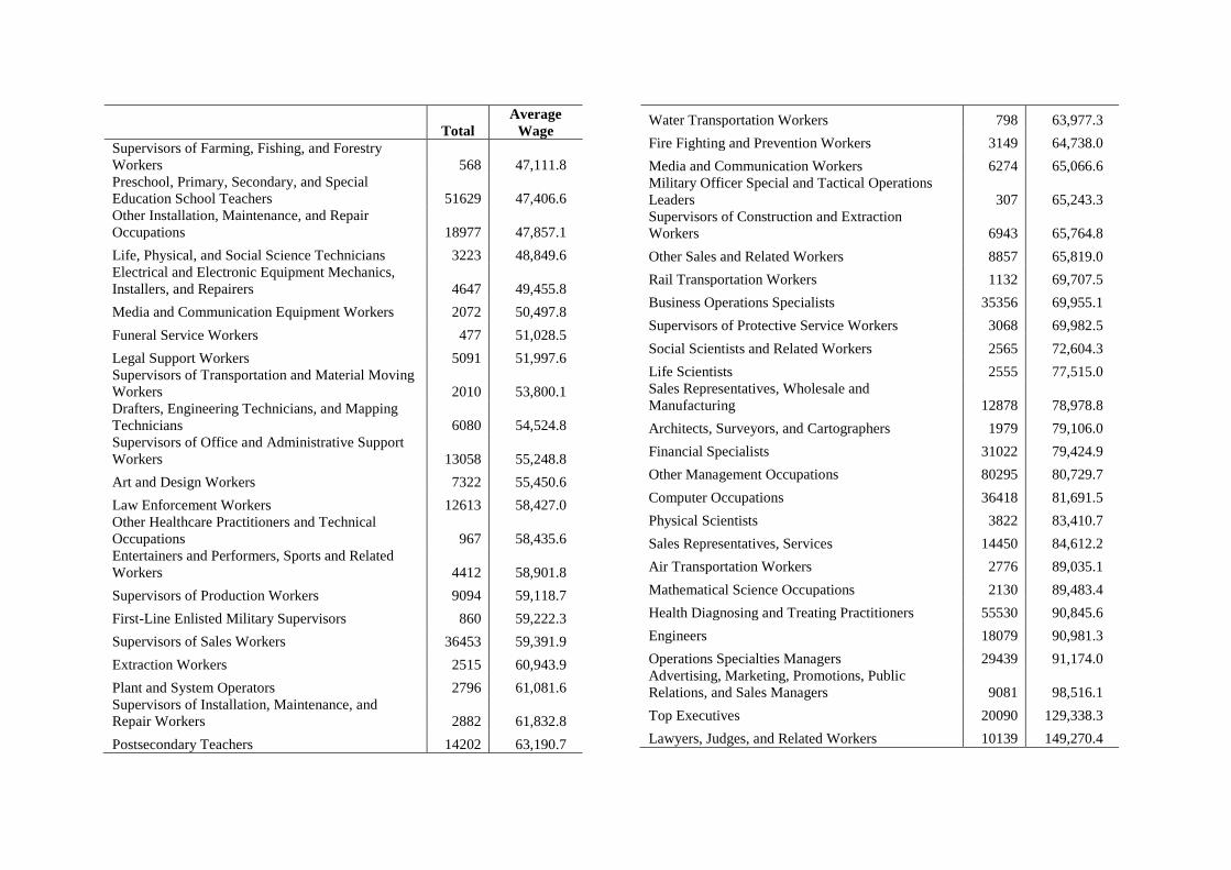
Table 3: Tabulation of Minor Occupations (Ordered by Average Wage) and Race

Total

Average

Wage

Other Food Preparation and Serving Related

Workers 3663 19,432.7

Cooks and Food Preparation Workers 17886 20,598.2

Food and Beverage Serving Workers 17433 21,854.4

Other Personal Care and Service Workers 16153 23,838.9

Other Education, Training, and Library Occupations 9926 25,886.9

Textile, Apparel, and Furnishings Workers 4343 25,898.8

Personal Appearance Workers 5886 26,041.6

Tour and Travel Guides 308 26,106.2

Nursing, Psychiatric, and Home Health Aides 14971 26,315.8

Agricultural Workers 7251 26,373.3

Grounds Maintenance Workers 7257 26,915.3

Building Cleaning and Pest Control Workers 25914 27,735.1

Animal Care and Service Workers 1358 28,155.2

Helpers, Construction Trades 365 29,673.7

Baggage Porters, Bellhops, and Concierges 688 29,769.0

Food Processing Workers 5416 29,860.0

Other Healthcare Support Occupations 10458 29,939.9

Retail Sales Workers 38779 30,690.8

Supervisors of Food Preparation and Serving

Workers 6939 30,949.4

Entertainment Attendants and Related Workers 1894 31,299.3

Material Moving Workers 28989 31,786.2

Woodworkers 1216 32,902.5

Assemblers and Fabricators 10300 33,499.4

Information and Record Clerks 39683 34,024.4

Other Transportation Workers 1980 34,543.0

Forest, Conservation, and Logging Workers 627 34,741.8

Communications Equipment Operators 644 34,853.0

Other Protective Service Workers 9707 35,564.3

Secretaries and Administrative Assistants 31855 35,721.4

Other Office and Administrative Support Workers 26881 36,375.9

Printing Workers 2045 36,429.0

Financial Clerks 23355 36,652.2

Material Recording, Scheduling, Dispatching, and

Distributing Workers 29096 36,732.1

Other Production Occupations 25972 38,780.3

Motor Vehicle Operators 36245 39,211.9

Military Enlisted Tactical Operations and

Air/Weapons Specialists and Crew Members 3695 39,632.7

Occupational Therapy and Physical Therapist

Assistants and Aides 922 40,125.9

Fishing and Hunting Workers 253 40,466.8

Construction Trades Workers 43972 40,649.6

Supervisors of Building and Grounds Cleaning and

Maintenance Workers 2720 41,769.4

Religious Workers 5932 41,867.4

Metal Workers and Plastic Workers 17126 41,912.9

Supervisors of Personal Care and Service Workers 729 42,889.8

Vehicle and Mobile Equipment Mechanics,

Installers, and Repairers 15090 43,224.4

Other Teachers and Instructors 5428 43,841.5

Counselors, Social Workers, and Other Community

and Social Service Specialists 17508 44,091.6

Health Technologists and Technicians 26264 44,153.5

Librarians, Curators, and Archivists 2551 44,950.8

Other Construction and Related Workers 3028 46,545.0

Total

Average

Wage

Supervisors of Farming, Fishing, and Forestry

Workers 568 47,111.8

Preschool, Primary, Secondary, and Special

Education School Teachers 51629 47,406.6

Other Installation, Maintenance, and Repair

Occupations 18977 47,857.1

Life, Physical, and Social Science Technicians 3223 48,849.6

Electrical and Electronic Equipment Mechanics,

Installers, and Repairers 4647 49,455.8

Media and Communication Equipment Workers 2072 50,497.8

Funeral Service Workers 477 51,028.5

Legal Support Workers 5091 51,997.6

Supervisors of Transportation and Material Moving

Workers 2010 53,800.1

Drafters, Engineering Technicians, and Mapping

Technicians 6080 54,524.8

Supervisors of Office and Administrative Support

Workers 13058 55,248.8

Art and Design Workers 7322 55,450.6

Law Enforcement Workers 12613 58,427.0

Other Healthcare Practitioners and Technical

Occupations 967 58,435.6

Entertainers and Performers, Sports and Related

Workers 4412 58,901.8

Supervisors of Production Workers 9094 59,118.7

First-Line Enlisted Military Supervisors 860 59,222.3

Supervisors of Sales Workers 36453 59,391.9

Extraction Workers 2515 60,943.9

Plant and System Operators 2796 61,081.6

Supervisors of Installation, Maintenance, and

Repair Workers 2882 61,832.8

Postsecondary Teachers 14202 63,190.7

Water Transportation Workers 798 63,977.3

Fire Fighting and Prevention Workers 3149 64,738.0

Media and Communication Workers 6274 65,066.6

Military Officer Special and Tactical Operations

Leaders 307 65,243.3

Supervisors of Construction and Extraction

Workers 6943 65,764.8

Other Sales and Related Workers 8857 65,819.0

Rail Transportation Workers 1132 69,707.5

Business Operations Specialists 35356 69,955.1

Supervisors of Protective Service Workers 3068 69,982.5

Social Scientists and Related Workers 2565 72,604.3

Life Scientists 2555 77,515.0

Sales Representatives, Wholesale and

Manufacturing 12878 78,978.8

Architects, Surveyors, and Cartographers 1979 79,106.0

Financial Specialists 31022 79,424.9

Other Management Occupations 80295 80,729.7

Computer Occupations 36418 81,691.5

Physical Scientists 3822 83,410.7

Sales Representatives, Services 14450 84,612.2

Air Transportation Workers 2776 89,035.1

Mathematical Science Occupations 2130 89,483.4

Health Diagnosing and Treating Practitioners 55530 90,845.6

Engineers 18079 90,981.3

Operations Specialties Managers 29439 91,174.0

Advertising, Marketing, Promotions, Public

Relations, and Sales Managers 9081 98,516.1

Top Executives 20090 129,338.3

Lawyers, Judges, and Related Workers 10139 149,270.4

Table 4: Tabulation of major occupations and race

Total

Average

Wage

Food Preparation and Serving Related Occupations 45921 22546.3

Personal Care and Service Occupations 27493 26188.3

Healthcare Support Occupations 26351 28237.3

Building and Grounds Cleaning and Maintenance Occupations 35891 28632.9

Farming, Fishing, and Forestry Occupations 8699 28740.5

Office and Administrative Support Occupations 164572 37275.9

Transportation and Material Moving Occupations 73930 39176.8

Production Occupations 78308 40444.9

Community and Social Service Occupations 23440 43528.7

Military Specific Occupations 4862 44714.9

Construction and Extraction Occupations 56823 44860.2

Education, Training, and Library Occupations 83736 47226.8

Installation, Maintenance, and Repair Occupations 41596 47323.4

Protective Service Occupations 28537 52588.9

Sales and Related Occupations 111417 55448.1

Arts, Design, Entertainment, Sports, and Media Occupations 20080 58702.4

Life, Physical, and Social Science Occupations 12165 70737.3

Business and Financial Operations Occupations 66378 74380.8

Healthcare Practitioners and Technical Occupations 82761 75649.3

Architecture and Engineering Occupations 26138 81602.0

Computer and Mathematical Occupations 38548 82122.1

Management Occupations 138905 91136.4

Legal Occupations 15230 116754.6

Table 5: Tabulation of States and Race

White Hispanic Black Asian

Native

American/

Pacific

Islander

Mixed

Race

Total

Alabama 12452 434 3444 183 71 160 16744

Alaska 1668 95 47 163 614 129 2716

Arizona 15014 5220 824 815 1152 423 23448

Arkansas 8045 484 1172 116 64 119 10000

California 62353 43876 6014 23047 1045 3593 139928

Colorado 17495 3090 649 565 147 409 22355

Connecticut 11818 1345 1147 676 23 199 15208

Delaware 2658 223 556 137 16 45 3635

District of Columbia 1649 268 1065 131 3 78 3194

Florida 44699 14750 8821 2096 164 911 71441

Georgia 23329 2407 8607 1371 76 395 36185

Hawaii 1449 326 116 2291 582 1159 5923

Idaho 4690 498 25 57 86 73 5429

Illinois 38299 5868 4224 2562 52 500 51505

Indiana 22738 1009 1430 403 46 223 25849

Iowa 11916 385 159 158 29 60 12707

Kansas 9683 727 383 233 87 217 11330

Kentucky 14568 384 935 195 28 154 16264

Louisiana 11053 675 3993 291 86 156 16254

Maine 4601 46 32 39 28 69 4815

Maryland 15832 1732 6169 1673 53 455 25914

Massachusetts 23618 1777 1448 1736 35 446 29060

Michigan 30493 1100 2659 830 221 446 35749

Minnesota 20821 527 488 564 218 230 22848

Mississippi 6113 222 2993 88 45 54 9515

Missouri 20163 567 1706 343 94 301 23174

Montana 3293 70 13 19 184 38 3617

Nebraska 7089 412 196 116 68 77 7958

Nevada 6140 2362 677 942 249 291 10661

New Hampshire 5543 104 60 120 9 59 5895

New Jersey 24214 5296 3768 3687 50 428 37443

New Mexico 2880 2512 101 98 932 83 6606

New York 52192 9234 8579 6280 196 1060 77541

North Carolina 26841 2260 6190 949 435 418 37093

North Dakota 2852 50 21 20 133 26 3102

Ohio 39407 1094 3511 811 60 550 45433

Oklahoma 9747 919 665 209 1215 836 13591

Oregon 12084 1216 173 598 199 365 14635

Pennsylvania 44496 1563 2741 1135 51 438 50424

Rhode Island 3673 391 185 125 11 56 4441

South Carolina 12601 654 3565 234 76 189 17319

South Dakota 3077 60 26 23 207 54 3447

Tennessee 19174 807 3093 397 53 278 23802

Texas 53533 29111 9188 4466 342 1368 98008

Utah 9127 998 76 260 162 129 10752

Vermont 2528 26 17 22 3 22 2618

Virginia 24846 2099 5246 2314 115 656 35276

Washington 21525 2262 739 2214 607 879 28226

West Virginia 5870 61 176 45 4 51 6207

Wisconsin 22040 680 604 370 174 190 24058

Wyoming 2153 152 14 16 71 32 2438

Table 6: Coefficients without Occupation Control

Female Hispanic Black Asian

Native

American/

Pacific

Islander

Mixed

Race

Alabama -0.378 -0.151 -0.185 -0.097 -0.182 -0.027

Alaska -0.284 -0.124 -0.307 -0.341 -0.302 -0.099

Arizona -0.270 -0.157 -0.180 -0.007 -0.189 -0.104

Arkansas -0.354 -0.082 -0.170 0.001 -0.114 -0.167

California -0.275 -0.223 -0.165 -0.119 -0.179 -0.119

Colorado -0.320 -0.126 -0.192 -0.050 -0.175 -0.042

Connecticut -0.354 -0.176 -0.202 -0.068 0.210 -0.066

Delaware -0.231 -0.092 -0.172 0.021 -0.207 -0.084

District of Columbia -0.125 -0.149 -0.310 -0.156 -0.259 -0.092

Florida -0.281 -0.165 -0.200 -0.103 -0.162 -0.106

Georgia -0.312 -0.179 -0.194 -0.083 -0.210 -0.059

Hawaii -0.248 -0.091 -0.036 -0.160 -0.208 -0.105

Idaho -0.376 -0.070 -0.147 -0.035 -0.181 -0.182

Illinois -0.338 -0.131 -0.125 -0.066 -0.127 -0.032

Indiana -0.358 -0.076 -0.150 -0.062 -0.089 -0.116

Iowa -0.342 -0.030 -0.259 0.028 -0.230 -0.150

Kansas -0.393 -0.064 -0.040 0.021 -0.104 -0.110

Kentucky -0.348 -0.128 -0.171 0.098 -0.191 -0.146

Louisiana -0.442 -0.165 -0.262 -0.030 -0.043 -0.169

Maine -0.318 0.012 0.020 -0.030 -0.061 -0.131

Maryland -0.272 -0.149 -0.101 -0.110 -0.033 -0.067

Massachusetts -0.343 -0.182 -0.169 -0.028 -0.042 -0.193

Michigan -0.353 -0.088 -0.111 0.063 -0.178 -0.146

Minnesota -0.333 -0.153 -0.198 0.013 -0.128 -0.090

Mississippi -0.353 -0.151 -0.254 0.026 -0.130 -0.131

Missouri -0.334 -0.048 -0.092 0.000 -0.129 -0.030

Montana -0.372 -0.115 -0.103 -0.128 -0.056 0.080

Nebraska -0.336 -0.093 -0.156 0.094 -0.261 -0.223

Nevada -0.234 -0.172 -0.193 -0.181 -0.141 -0.055

New Hampshire -0.394 -0.049 -0.190 -0.024 -0.030 -0.064

New Jersey -0.347 -0.250 -0.162 -0.062 -0.254 -0.111

New Mexico -0.295 -0.111 -0.133 -0.020 -0.172 0.009

New York -0.280 -0.125 -0.099 -0.096 -0.107 -0.081

North Carolina -0.316 -0.188 -0.189 0.020 -0.161 -0.095

North Dakota -0.447 -0.088 -0.566 -0.243 -0.112 -0.110

Ohio -0.327 -0.126 -0.151 0.046 -0.213 -0.040

Oklahoma -0.390 -0.102 -0.157 -0.038 -0.088 -0.037

Oregon -0.314 -0.181 -0.066 0.044 -0.152 -0.102

Pennsylvania -0.340 -0.082 -0.108 0.008 -0.005 -0.034

Rhode Island -0.338 -0.191 -0.235 -0.014 -0.020 -0.083

South Carolina -0.318 -0.222 -0.222 -0.126 -0.014 -0.136

South Dakota -0.334 -0.129 -0.264 -0.269 -0.248 -0.071

Tennessee -0.330 -0.121 -0.177 0.030 -0.040 -0.106

Texas -0.367 -0.210 -0.228 -0.074 -0.163 -0.105

Utah -0.428 -0.143 -0.225 -0.087 -0.086 0.005

Vermont -0.287 0.015 -0.104 -0.224 -0.098 -0.415

Virginia -0.342 -0.097 -0.158 -0.053 -0.083 -0.014

Washington -0.345 -0.166 -0.131 -0.016 -0.119 -0.047

West Virginia -0.365 -0.060 -0.057 0.007 0.070 -0.157

Wisconsin -0.339 -0.126 -0.223 0.017 -0.124 -0.073

Wyoming -0.458 -0.231 0.151 0.031 -0.285 -0.091

Table 7: Coefficients with Occupation Control

Female Hispanic Black Asian

Native

American/

Pacific

Islander

Mixed

Race

Alabama -0.326 -0.097 -0.110 -0.069 -0.150 -0.026

Alaska -0.206 -0.069 -0.219 -0.228 -0.254 -0.057

Arizona -0.218 -0.078 -0.095 -0.023 -0.067 -0.068

Arkansas -0.299 -0.028 -0.109 -0.042 -0.078 -0.119

California -0.207 -0.134 -0.091 -0.101 -0.124 -0.092

Colorado -0.252 -0.073 -0.107 -0.051 -0.116 -0.034

Connecticut -0.285 -0.098 -0.110 -0.035 0.202 -0.042

Delaware -0.241 -0.071 -0.106 0.012 -0.098 0.010

District of Columbia -0.114 -0.085 -0.229 -0.149 -0.090 -0.007

Florida -0.254 -0.107 -0.108 -0.093 -0.136 -0.072

Georgia -0.272 -0.103 -0.114 -0.097 -0.164 -0.043

Hawaii -0.184 -0.047 -0.063 -0.069 -0.095 -0.030

Idaho -0.295 -0.034 -0.051 0.000 -0.104 -0.124

Illinois -0.271 -0.070 -0.049 -0.063 -0.074 0.002

Indiana -0.293 -0.032 -0.074 -0.053 -0.021 -0.071

Iowa -0.271 -0.002 -0.165 0.023 -0.221 -0.190

Kansas -0.326 -0.018 0.016 0.006 -0.061 -0.092

Kentucky -0.277 -0.093 -0.088 0.034 -0.165 -0.115

Louisiana -0.364 -0.095 -0.156 0.039 -0.010 -0.133

Maine -0.254 0.058 0.097 -0.032 0.000 -0.093

Maryland -0.220 -0.067 -0.045 -0.090 -0.019 -0.049

Massachusetts -0.287 -0.096 -0.075 -0.040 0.017 -0.134

Michigan -0.281 -0.027 -0.054 0.015 -0.112 -0.108

Minnesota -0.269 -0.075 -0.112 0.007 -0.059 -0.054

Mississippi -0.295 -0.071 -0.154 0.053 -0.077 -0.139

Missouri -0.273 -0.004 -0.038 -0.002 -0.094 -0.027

Montana -0.312 -0.070 -0.119 -0.203 0.008 0.028

Nebraska -0.260 -0.074 -0.081 0.062 -0.205 -0.210

Nevada -0.198 -0.084 -0.121 -0.119 -0.110 -0.036

New Hampshire -0.333 -0.026 -0.027 -0.058 -0.011 -0.070

New Jersey -0.276 -0.150 -0.093 -0.072 -0.150 -0.108

New Mexico -0.194 -0.059 -0.088 -0.031 -0.089 0.044

New York -0.225 -0.047 -0.022 -0.065 -0.074 -0.048

North Carolina -0.278 -0.110 -0.102 0.001 -0.101 -0.090

North Dakota -0.295 -0.087 -0.449 -0.227 -0.076 -0.136

Ohio -0.275 -0.091 -0.078 0.016 -0.105 -0.016

Oklahoma -0.310 -0.031 -0.075 -0.035 -0.053 -0.012

Oregon -0.250 -0.094 0.023 0.049 -0.096 -0.088

Pennsylvania -0.286 -0.028 -0.030 -0.014 0.005 -0.015

Rhode Island -0.307 -0.123 -0.158 -0.003 0.006 -0.066

South Carolina -0.284 -0.144 -0.133 -0.105 0.044 -0.106

South Dakota -0.284 -0.061 -0.241 -0.152 -0.166 -0.018

Tennessee -0.293 -0.065 -0.093 0.036 -0.023 -0.096

Texas -0.288 -0.134 -0.139 -0.086 -0.093 -0.057

Utah -0.352 -0.082 -0.169 -0.060 -0.047 -0.010

Vermont -0.242 -0.030 -0.123 -0.155 0.154 -0.327

Virginia -0.257 -0.032 -0.085 -0.057 -0.052 -0.001

Washington -0.256 -0.072 -0.051 -0.006 -0.065 -0.019

West Virginia -0.252 -0.052 0.022 0.018 0.060 -0.117

Wisconsin -0.272 -0.071 -0.139 0.019 -0.105 -0.059

Wyoming -0.339 -0.137 0.194 0.204 -0.173 -0.010