Gender and occupational wage gaps in Romania - DiVA …oru.diva-portal.org/smash/get/diva2:174727/FULLTEXT01.pdf · Gender and occupational wage gaps in Romania: ... the Communist

Gender and occupational wage gaps in Romania:

from planned equality to market inequality?∗

Daniela Andrén

School of Business, Economics and Law at Göteborg University Department of Economics

Box 640, SE 405 30 Göteborg Sweden

Email: [email protected]

Thomas Andrén School of Business, Economics and Law at Göteborg University

Department of Economics Box 640, SE 405 30 Göteborg

Sweden and

IZA, Bonn [email protected]

Abstract In Romania, the communist regime promoted an official policy of gender equality for more than 40 years, providing equal access to education and employment, and restricting pay differentiation based on gender. After its fall in December 1989, the promotion of equal opportunities and treatment for women and men did not constitute a priority for any of the governments of the 1990s. This paper analyzes both gender and occupational wage gaps before and during the first years of transition to a market economy, and finds that the communist institutions did succeed in eliminating the gender wage differences in female- and male-dominated occupations, but not in gender-integrated occupations.

∗ We thank seminar participants at Göteborg University and Växjö University for useful comments, and the Swedish

Research Council for financial support.

1 Introduction

In Romania, the communist regime proclaimed from its establishment in the middle of the

1940s that liberty, gender equality and the emancipation of women were some of the main

targets in the development of the new socialist society. A nationwide campaign was

launched in order to eliminate female illiteracy, to increase the enrollment of women in

secondary schools and universities, and to increase female employment outside of the

household. Although all “able-bodied” citizens of working-age had the right and duty to

work and were guaranteed a job, labor markets in particular were subject to a number of

constraints, including a strict regulation of mobility, central allocation of university

graduates to jobs, and a centralized wage-setting process. Additionally, from 1966, women

were required to have more children. Hence, it does not seem likely that the communist

regime could have reached its targets. However, the statistics show that by its fall in

December 1989, at least some of the communist regime’s targets regarding in particular the

emancipation of women and gender equality in general had indeed been achieved.1

Before December 1989, the institutional support for women rights was strong.

Romania ratified the United Nations Convention on the Elimination of All Forms of

Discrimination Against Women on January 7, 1982. The Constitution of the Socialist

Republic of Romania, adopted in 1965, states that “women and men have equal rights”,2

and the new constitution, adopted in 1991 and modified in 2003, reinforces “equal pay for

equal work” (or mot à mot, “on equal work with men, women shall get equal wages”).3

However, under central planning, wages were set according to industry-specific wage grids

varying only with the difficulty of the job and with worker education and experience, and

not with gender. Given that the promotion of equal opportunities and treatment did not

1 The most impressive achievement was that of the literacy rates. While in 1945, only 27% of the population were unable to read or write, in 1989, the literacy rates were 95.6% for women, and 98.6% for men (UNESCO, 2002; 2005). Another impressive achievement is the relatively high and gender neutral proportion of young people who were enrolled in high schools or universities in 1988/89: a) about 70% of males aged 15-19 years, and about 72% of females in the same age interval were enrolled in high school education; b) about 6% of both males and females aged 19-25 years were enrolled in some form of higher education (National Commission for Statistics, 1995). Nevertheless, the workforce participation rates were unusually high relative to Western standards for both women (about 90-95% during the 1970s and 1980s), and men, approached 100 percent (Central Statistical Direction). 2 “In Republica Socialista Romania, femeia are drepturi egale cu barbatul.” (Art. 26). 3 “La munca egala, femeile au salariu egal cu barbatii.” (Art. 38, §4 from 1991, and Art. 41, § 4 from 2004).

3

constitute a priority for any of the governments of the 1990s (United Nations, 2003),4 the

question is how much the communist setting of gender equality was affected by the

economic and social downturns of the transition years.

Previous research on other transition economies found that the gender wage gap

generally decreases in the transition process. Given the similarities between the Romanian

economy and the other transition economies from Central and Eastern Europe, especially

in terms of issues related to gender equality, it was not unexpected that the gender wage gap

in Romania reached similar levels in the first years of transition (Paternostro and Sahn,

1999; Skoufias, 2003). The contribution of this study is not only the analysis of the wage

gap during the communist regime and during the first ten years of transition, but also the

use of a structural approach that controls for occupational attainment and institutional

settings. The main hypothesis is that the process of labor reallocation caused by the

economic transition had an impact not only on the occupational distribution of women

and men, but also on the gender wage gap and the occupational wage gap. Therefore, we

analyze not only the gender wage gap, as previous studies on Romanian data, but also the

wage gap between occupations in general, but also separately for men and women. The

results from different regimes characterized by different settings and interventions suggest

that public policies aimed to decrease the gender wage gap should focus more on

redistributing labor or redirecting potential labor market entrants across occupations.

The study is organized in the following way. Section 2 presents some aspects related

to gender equality in Romania during the communist regime and the transition period, and

Section 3 describes the empirical specification. The data and the samples used in this study

are presented in Section 4, while the results are presented in Section 5. Section 6 contains a

summary of the paper with some policy implications.

2 The gender issues and the institutions

The gender equality actions in Romania were developed during the communism era when

“liberty”, gender equality, and the emancipation of women were emphasized in the

4 In 2000, the last year of the available data, a special Commission for Equal Opportunities was established. The new Romanian Constitution, modified in 2003, states that “everyone has the free choice of profession and workplace”, and reinforces the guarantee for equal opportunities for women and men in gaining access to a public office or dignity, civil or military. However, in 2003, there was a major gap between policy and practice, with women earning less, being concentrated in low-paid sectors and under-represented in management (Vasile, 2004).

4

constitution as well as in other official documents (e.g., the Communist Party’s decisions,

laws and decrees). During the second half of the 1940s when communism was imposed in

Romania, the society was predominantly rural with a strong mentality towards the woman

as the crucial “factor” of the family. Therefore, it was impossible to imagine that Romanian

women could engage in work outside the household in general, and especially in work

considered to be suitable for men only. However, in the 1950s, this aspect of gender

equality in the economy was evoked in party speeches by the presence of “women heroes”

working in areas which had typically been male-dominated: from working in mines

underground, or in industrial, chemical and metallurgical operations, to professions in areas

such as surgery and experimental sciences (Vese, 2001). Furthermore, the state launched a

nationwide campaign to virtually eliminate female illiteracy and to increase the enrollment

of women in secondary schools and universities. At the same time that these changes were

being put into place, the state was demanding that women have more children. This was

done through different regulations, such as a fertility policy that banned abortion and

limited contraception; the introduction of a tax on adults older than twenty-five years,

single or married, who were childless; and the offering of a number of positive incentives to

increase births, e.g., parents of large families were given additional subsidies for each new

birth, families with children were given preference in housing assignments, the number of

child care facilities were increased, and maternal leave policies were put into place (Keil and

Andreescu, 1999).

Beginning in 1951, Romania set into practice the Soviet system of central planning

based on five-year development cycles. The development program assigned top priority to

the industrial sector (the machinery, metallurgical, petroleum refining, electric power, and

chemical industries), necessitating a major movement of labor from the agriculture

occupations in the countryside to industrial jobs in newly created urban centers. The labor

market was characterized by a centralized wage-setting process with a standard set of rules

based on industry, occupation, and length of service (Earle and Sapatoru 1993). Wages

were set according to industry-specific wage grids varying only with the difficulty of the job

and with the worker’s education and experience, not with gender. After the fall of

communism, in December 1989, the new wage law of February 1991 formally

decentralized wage determination in Romania. All state and privately owned commercial

5

companies were granted the right to determine their wage structure autonomously through

collective or individual negotiations between employees and employer. Pay was no longer

tied to performance as it has been during the years of socialism, and all restrictions on

eligibility for promotion, bonuses, and internal and external migration were lifted. Also,

hours of work per week were reduced from 46 to 40 without any decrease in monthly

wages (Skoufias, 2003).

The structural starting point of the economic transformation was an oversized state-

owned industry characterized by low competition and weak interaction with the world

market. Despite still being the majority owner, the state did not intervene with any policy

regarding wage differentials. Instead, its interventions have been limited to periodic

indexations. Nevertheless, the state allowed sometime specific indexations only for the state

institutions in order to diminish an increasing gap caused by the more rapid wage increases

in the some industries because of negotiations of the collective and individual contracts.

This system was supplemented by price liberalization and privatization, financial crises and

a lack of (rule of) laws. All these factors have an effect on the labor market participation,

occupational attainment and, nonetheless, on people’s opinion about their opportunities

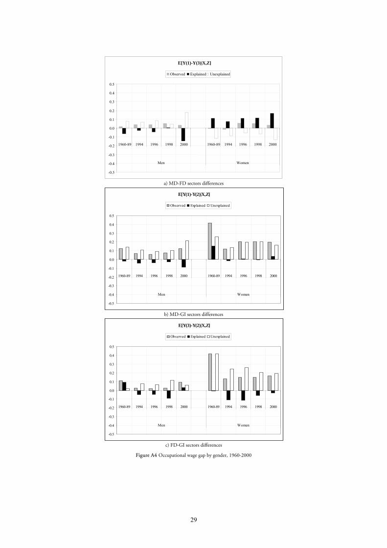
and their place on the labor market. The 2000 Gender Barometer indicates that about half

of those interviewed answered that it does not exist real equality of rights between women

and men.5 A majority (about 75-88%) considered gender not to be important in some

occupations with respect to who should be employed (e.g., media, nongovernmental

organizations, public administration, health, agriculture and banking), but that men should

be employed in mining and metallurgy and construction, and women should be employed

in the textile industry. See Table A1 in the Appendix.

3 Empirical framework

The earlier literature on wage differentials suggests that the fact that occupations differ in

average wage rate enhances and distorts the overall wage differentials between groups of

people. Controlling for individual characteristics and observed occupational choice is not

enough to hedge this distortion, and therefore we formulate a selection model with an

5 The Gender Barometer of the Open Society Foundation covers a representative sample of 1,839 persons aged 18 and over, and it is the first documented attempt to examine the Romanian society in terms of the roles of women and men, their relationships, and their everyday life.

6

endogenous switch among three broad types of occupational groups.6 Within this

framework, a given individual could be in any of the three sectors, and each sector has its

own wage-generating function that will depend on the observed and unobserved

characteristics of the individual, everything else equal. To analyze the wage differences

among the sectors for a given individual requires formulating an wage equation for each

sector:

111 UXY += β male-dominated (MD) occupations, (1)

222 UXY += β gender-integrated (GI) occupations, (2)

333 UXY += β female-dominated (FD) occupations, (3)

where Yj is the market wage for sector j, ;3or2,1=j sector 1 represents the male-

dominated (MD) occupations, sector 2 the gender-integrated (GI) occupations, and sector

3 the female-dominated (FD) occupations X is a matrix of explanatory factors for the

market wage, and βj is the associated parameter vector, which is unique for each sector.

The occupational choice is based on the taste or the propensity for a specific

occupation: male dominated (i.e., occupation with a high density of men), gender

integrated, and female-dominated (i.e., occupation with a low density of men). The choice

mechanism is specified as a linear latent variable model:

εγ += ZD * , (4)

where Z is a matrix containing observed factors that determine the size of the occupational

propensity score, and γ is the associated parameters vector of these factors. The dependent

latent variable D* represents the propensity to choose a male-dominated occupation. A low

value of D* represents a low propensity to choose a male dominated occupation, which

should be seen as equivalent to a high propensity to choose a female-dominated

6 Several papers analyze the occupational segregation and wages by estimating the effect of women’s density in different occupations on individual wages. A potential problem in these studies is the endogeneity of occupational choice. Except for a few studies that do take this problem into account, e.g., Hansen and Wahlberg (2007), Macpherson and Hirsch (1995), Sorensen (1989; 1990), and England et al. (1988), most of the literature is based on the assumption that occupational attainment is exogenous.

7

occupation. If the latent variable takes a value between a high and a low value, the

individual will choose an occupation from the gender-integrated sector. The observed

counterpart of the latent variable is defined as:

(FD)

(GI)

(MD)

c if3

ccif2

c if1

2*

2*

1

1*

⎪⎩

⎪⎨

⎧

>≤≤<

=D

D

D

D <=> ⎪⎩

⎪⎨

⎧

−>−≤≤−

−<=

γεγεγ

γε

Zc

ZcZc

Zc

D

2

21

1

if3

if2

if1

, (5)

with 1c and 2c being two unknown break points that will be estimated, and may be

interpreted as intercepts, since Z does not include any constant.

The model, as defined by equations (1)-(5), contains four stochastic components

that presumably are related to each other if the occupational choice is endogenous. We

assume that these components are i.i.d. drawings from a multivariate normal distribution,

i.e., ( ) ( )Σ,~N,,U,UU 0321 ε . In principle, one can allow for any potential correlation

among the stochastic components. However, for a given individual, we only observe the

actual wage and the indicated occupational choice in pairs, and not simultaneously with

wages in other sectors. Therefore, the observability is partial, and we have to make inference

on the population based on marginal distributions that correspond to the observed data. In

particular, )1,εCov(U , ),( 2 εUCov and ),( 3 εUCov are identified by the data and are

therefore allowed to be non-zero, while the covariances among the residuals from the

output equations, )21,UCov(U , )31,UCov(U and )32,UCov(U , are left unspecified. The

variances of the output equations equations, )( 1UVar , )( 2UVar and )( 3UVar , are

identified, and we choose to normalize the variance of the residual of the selection equation

to 1.

In order to form the likelihood function, we make use of the marginal bivariate

normal density functions for ),,( 1 εU ),,( 2 εU and ),( 3 εU , and define the following

indicator variables

⎩⎨⎧ =

=elsewhere0

1 if11

Dδ ,

⎩⎨⎧ =

=elsewhere0

2 if12

Dδ ,

⎩⎨⎧ =

=elsewhere0

3 if13

Dδ .

8

Using this information, we construct the following likelihood function

∏ ∫∫∫=

∞

−

−

−

−

∞− ⎥⎥⎦

⎤

⎢⎢⎣

⎡

⎥⎥⎦

⎤

⎢⎢⎣

⎡⎥⎦

⎤⎢⎣

⎡=

N

i Zciii

Zc

Zciiii

Zc

ii

i

i

i

i

dUfdUfdUfL1

321

3

2

22

1

11

),(),(),(

δ

γ

δγ

γ

δγ

εεεεεε .

The conditional expectation of the wage residuals from each of the three sectors tells

us whether there is a positive or a negative selection into the analyzed sector, and they are

given by the following expressions

[ ] [ ]44 344 21

Negative

ZcEUCovDXUE γεεε −<×== 111 |),(1,| , (6)

[ ] [ ]4444 34444 21

negativePositive

ZcZcEUCovDXUE/

2122 |),(2,| γεγεε −≤≤−×== , (7)

[ ] [ ]444 3444 21

Positive

ZcEUCovDXUE γεεε −>×== 233 |),(3,| . (8)

Given that the sign of the second term of the product in Equations (6) and (8) does

not change, it is the sign of the covariance that determines the sign of the conditional

expectations. This means that if 0),( 1 >εUCov and 0),( 3 <εUCov , then we will find a

positive selection effect of the occupational sector on wage. In equation (7), on the other

hand, the covariance is just one of several factors determining the direction of the selection.

The estimates are used to compute the components of the gender wage gap for the whole

sample (i.e., all occupations together) and by occupational sector (i.e., MD, GI and FD

occupations), as well as the occupational wage gap for women and men separately.7

4 Data

The data used in the empirical analysis is drawn from the Romanian Integrated Household

Survey (RIHS). For the socialist years, 1960-1989, we use retrospective information in the

1994 survey, and for the analyzed transition years, we use the annual household survey

7 See Andrén and Andrén (2007) for a detailed description of the decomposition and each of its components.

9

(1994, 1996, 1998, and 2000).8 The number of observations that include information

about the wages and explanatory variables relevant for analysis vary across the cross-

sections, starting at 25,565 in 1994, increasing to 21,518 in 1998, and decreasing to

17,480 in 2000. The labor force history’s data contains about 12,000 individuals.

The net monthly wage is computed as earnings on the primary job in the previous

month minus taxes and other mandatory contributions. The wage variable refers to the

previous month from 1994 to 2000 and to the starting wage from 1950 to 1989. Our

concern are gender and occupational wage gaps rather than the overall level of real wages,

so that our approach of estimating repeated cross-sections involves no deflation of the

dependent variable. Nevertheless, the significant inflation during the 1990s requires some

within survey period adjustments, for which we use monthly dummies. The evolution of

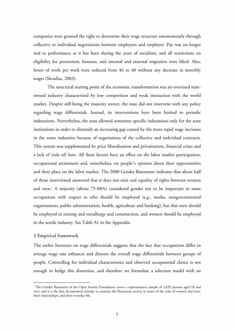
women’s net monthly wages relative to men’s varies between 84% in 1971-75 and 91%

during 1986-89 (Figure A1 in the Appendix). Compared to the female-male wage ratio

reported by Brainerd (2000), the Romanian values are near to those in Columbia (85% in

1988) and Sweden (84% in 1992), but much higher than those in USA (70% in 1987) and

the Russian republic (69% in 1989).

The next important variable in our analysis is occupation. Using a conventional

approach that splits occupations into three groups based on the proportion of female

workers in the occupation,9 we define occupations with less than 33% women as being

male-dominated occupations and occupations with more than 67% women as being

female-dominated category. The remaining occupations form the gender-integrated

occupations category.10 The highest difference between women and men wages was in the

gender-integrated sector, the women’s net monthly wages being about 80% of the men’s

during transition years. The smallest difference was in female-dominated sector, where

women earn on average about 90-95% of men’s monthly wages during 1981-1996 (Figure

A1 in the Appendix).

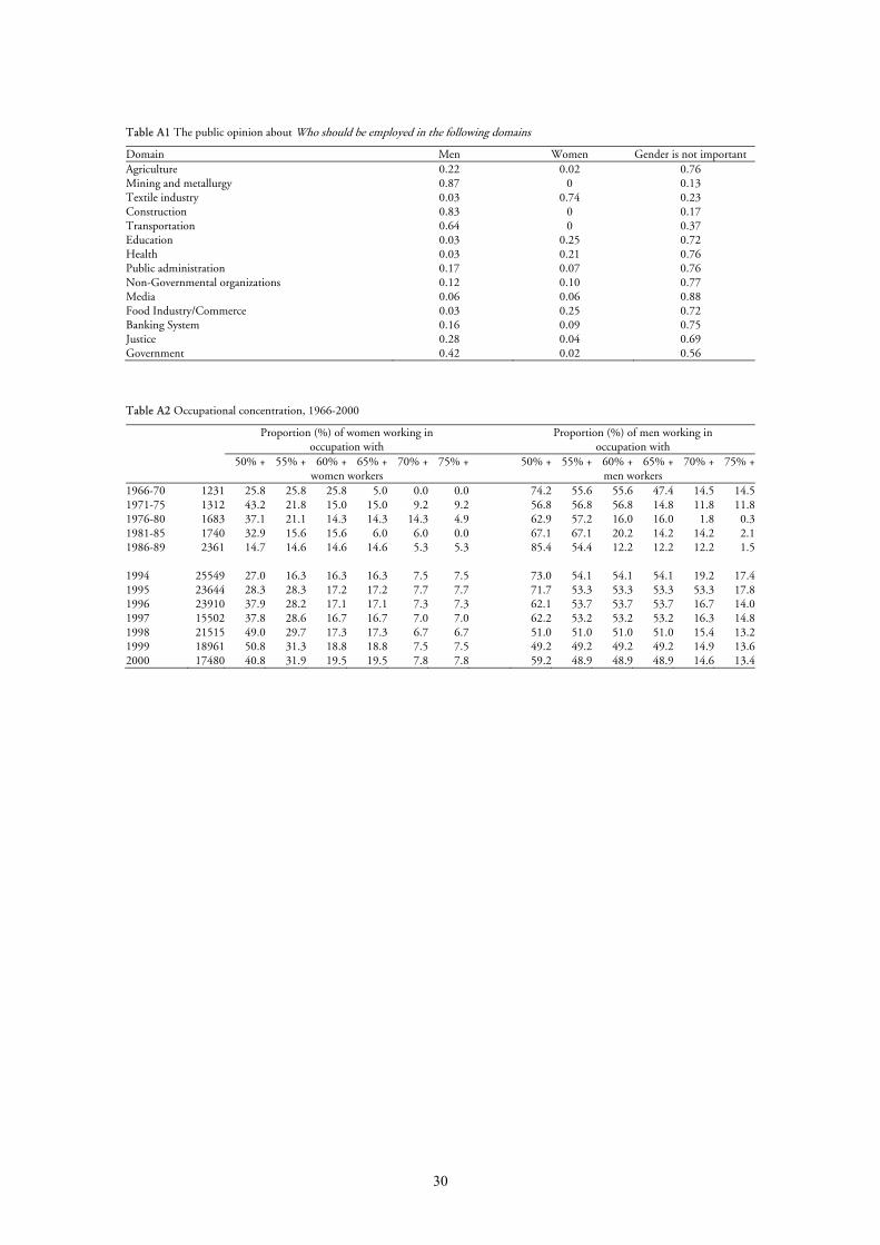
8 We analyzed all cross-sections (1994-2000), but we report results for every second year. Unfortunately, although originally designed as a panel, the data do not permit linking of individual observations across all years. 9 See Jacobs (1995) for details about occupational groups. 10 The distribution of individuals across these three groups was almost the same when we chose another cutting point (e.g., 25%, 30%, 35%). Figure A3 shows the evolution of these groups during 1951-2000. We divide the period before 1990’s into 5-year periods that overlap five-year development plans. Table A2 shows the proportion of women working in occupations with more than 50%, 60%, 70%, 80% and 90% women, and the same figures for men. Tables A3-A5 in the Appendix present basic descriptive statistics (by gender) for some variables used in the empirical analysis.

10

During the period before 1989, the relative differences between net monthly wages

between the three occupational sectors suggest that there was a moving trend towards

equalization of occupational wage differences for both women and men (Figure A2 in the

Appendix). Regardless their gender, those working in male-dominated occupations earned

more than those working in gender-integrated occupations, but this relationship switched

direction after 1994, and increased again during 1996 and 1997. Furthermore, the

evolution of the relative differences in the occupational wage gap during transition years

was different for women and men, suggesting that the market mechanisms can

occupational wage differences. The occupational differences were larger for women than for

men after 1994. For men, there is basically no difference between gender-integrated and

female-dominated occupations, while women working in the sector of female-dominated

occupations earn less than women working in the sector of gender-integrated occupations.

Another group of variables, important in analyzing the effect of occupational

selection on the domain-specific wages were the instruments for occupational choices.

Concerning this, it is generally difficult to obtain observable characteristics that influence

occupational choice but not wages. Analyzing data for several years characterized by

different structural changes in the economy makes it even harder to find instruments that

work well for both women and men for all years. Nevertheless, the institutional settings

during the analyzed period suggest that the wage differentiation based on gender was

restricted under central planning, and even in the beginning of the transition period. Wages

were set according to industry-specific wage grids varying only with the difficulty of the job

and with worker education and experience, and not with gender. Additionally, under the

central plan, given their last completed level of schooling and their ranking (based on

academic grades and political, cultural and even sportive involvement), people could choose

from a given and very limited list of jobs, sometimes restricted only to the municipality or

county area. Therefore, we argue that last completed level of schooling is an exogenous

source of variation in occupational attainment that allows us to identify the causal effect of

occupation. More exactly, after finishing compulsory education (i.e., 8 years of schooling),

people had to pass a test in order to continue their education at the high school level. A

majority of those who did not pass the test instead continued into vocational schools (most

of the time, being vocational programs of 1-2 years at the working place). Those who

11

passed the test were admitted to high school (lyceums), which could be general (e.g.,

mathematics-physics, natural sciences, and philosophy-history), specialized (e.g., economic,

pedagogical, health care, and art), industrial or agro-industrial. After two years of high

school, students had to pass a new test in order to continue the last two years of high

school. When finishing these two additional years, students had to pass another set of tests

in order to receive high school diploma. Only those who had high school diploma could

then take the university admission test (the university education was 3-6 years). High

school graduates who were not admitted at university usually did not have many

occupational choices; only few (usually those who graduated from a specialized high school)

had a certain situation regarding their occupation (e.g., nurses, teachers in the pre-school

and primary education). From those who were not admitted at university, graduates from

general high schools had on average better academic merits and their human capital were

better off on average than their peers who had graduated from other high schools, but there

were no clear rules for who would get the most attractive job. Sometimes they had to

compete even with their peers who graduated a shorter vocational program (from

vocational schools) and worked for a while. These are some of the institutional settings that

suggest that wages were related to the occupation, as a combination of factors such as

education, job, and task-specific requirements during the analyzed years (both before 1989,

and the first years of the transition). Due to this combination, it happened that people in

different occupations with different level of education had almost the same salary. Hence,

in order to control for the effect of the education on wages and occupational attainment,

respectively, we use two different groups of educational dummies. The first group, used in

the wage equations, includes three variables: lower, medium and higher, while the second

group, used in the selection equation, includes five variables: compulsory, vocational, high

school, post-high school, and university. The “lower” category in the wage equation covers

the “compulsory” (which can be 4 or 8 years) and “vocational” in the selection equation,

while “medium” covers “high school” and “post-high school”; and “higher” is the same as

“university”. Due to these differences, we use the “vocational”, “2 or 4 years high school”,

and “post high school” as instruments. In addition to these instruments, we use three

dummies that should control for occupational “specialization” within ethnic groups

[(Borjas (1992; 1995), Lehrer (2004)]. We control for this effect through geographical

12

regions. Following the same strategy as for education, the regions are aggregated in different

groups of dummies: (i) four dummies for the richest geographical regions (R4-R8), in the

wage equations; and (ii) five dummies for regions with a big majority of ethnic Romanians

(R1-R4 and R8) in comparisons with the regions with a relatively higher proportion of

other ethnicities, mainly ethnic Hungarians,11 in the selection equation.

5 Results

We estimate a selection model with an endogenous switch among three broad types of

occupational groups defined by their gender composition: male-dominated, gender-

integrated, and female-dominated occupations. The parameters for the occupational

selection equation and the domain-specific wage equations were estimated simultaneously.

5.1 Selection into occupational groups

The parameters for the occupational selection equation and the domain-specific wage

equations were estimated simultaneously. Table 1 presents the estimates of the selection

equations for women and men, respectively.12 Additionally, we present the variances and

some covariances of error terms of the wage and selection equations, which provide useful

information regarding the sorting behavior of individuals across sectors.

The estimated coefficients of the occupational selection (or attainment) equation

indicate that the probability to work in a given occupational group (i.e., MD, GI or FD)

differs between women and men. Even though it is not possible to pinpoint a clear trend, it

seems that men’s preferences for a given occupation were more stable than women’s.

Women’s correlations between observables and occupational choice are less stable over

time. However, when these correlations are statistically significant, they suggest that women

changed preferences during transition years. The differences between women and men

during the communist era might be due to the big changes in the economy during that

time (such as industrialization, mass privatization of the agriculture, prohibition of

abortion, etc.), while the differences during the transition years might indicate the collapse

11 See Andrén (2007) for a detailed description and analysis of wage differences between ethnic Romanians and ethnic Hungarians. 12 Tables A6 and A7 in the Appendix present the estimates of domain-specific (i.e., MD, GI and FD) wage equations for women and men respectively.

13

of the socialist support for women but also the changes in the economy and society, which

might have changed women’s work preferences and/or opportunities.

Table 1 Selection equation estimates, by gender, 1960-2000

Women Men

1960- 89 1994 1996 1998 2000 1960- 89 1994 1996 1998 2000c1 -0.894 *** -0.510 ** -1.072 *** -1.345 *** -0.682 ** -1.285 *** -0.938 *** -0.544 *** -0.610 *** -0.754 *** c2 2.138 *** 2.112 *** 1.658 *** 1.547 *** 2.149 *** 1.595 *** 1.698 *** 2.174 *** 2.214 *** 1.931 *** Age 0.425 *** 0.365 *** 0.004 0.000 0.274 * -0.119 -0.303 *** -0.008 0.029 -0.009 Age2/10 -0.049 ** -0.034 ** 0.014 0.005 -0.024 0.026 0.048 *** 0.007 0.003 0.012 Educational Level1)

Vocational 0.113 * 0.222 *** 0.219 *** 0.253 *** 0.182 *** -0.128 ** 0.155 *** 0.105 *** 0.097 *** -0.255 *** High school 2 years# 0.766 *** 0.802 *** 0.173 *** 0.226 *** 0.273 *** 0.208 *** 0.372 *** 0.034 0.139 *** -0.172 *** High school 4 years 0.934 *** 0.975 *** 0.932 *** 0.403 *** 0.421 *** -0.017 After high school 0.922 *** 0.718 *** 0.805 *** 1.066 *** 1.033 *** 0.719 *** 0.689 *** 0.634 *** 0.652 *** -0.546 *** University 0.163 0.159 *** 0.296 *** 0.347 *** 0.343 *** 0.076 0.470 *** 0.381 *** 0.466 *** 0.065

Region R1: North-East -0.101 * -0.174 *** -0.185 *** -0.240 *** -0.173 *** -0.010 -0.107 *** -0.182 *** -0.151 *** 0.033 R2: South-East -0.067 -0.008 -0.087 ** -0.151 *** -0.101 ** -0.277 *** 0.047 -0.047 -0.110 *** -0.183 *** R3:South 0.057 -0.114 *** -0.072 * -0.122 *** -0.094 ** -0.145 ** -0.064 ** -0.140 *** -0.128 *** -0.089 ** R4: South-West -0.017 -0.075 * -0.162 *** -0.200 *** -0.215 *** 0.007 -0.050 -0.086 ** -0.076 * 0.019 R8: Bucharest 0.154 * -0.090 ** -0.050 -0.055 -0.089 * -0.023 0.096 ** 0.043 -0.025 -0.099 **

Hungarians*Center -0.225 -0.403 -0.150 0.242 -0.434 -0.761 -0.287 -0.185 0.101 -0.428 Married -0.046 -0.013 0.031 -0.030 0.004 -0.046 -0.127 *** -0.105 *** -0.225 *** -0.071 * Urban -0.109 ** 0.072 ** -0.020 -0.056 -0.014 0.034 0.032 -0.009 0.026 0.082 *** Ethnicity2)

Romanian -0.234 * -0.083 -0.025 -0.003 -0.015 -0.212 * -0.042 -0.053 -0.154 * -0.009 Hungarian 0.048 0.330 0.067 -0.201 0.404 0.635 0.255 0.060 -0.196 0.575

Sector 3) Agriculture -0.538 *** -0.563 *** -0.327 *** -0.208 ** -0.523 *** -0.457 *** -0.352 *** -0.437 *** Industry -0.565 *** -0.477 *** -0.428 *** -0.433 *** 0.127 *** 0.217 *** 0.227 *** 0.116 ***

Private ownership 0.406 *** 0.046 0.034 -0.040 -0.135 *** -0.179 ** 0.138 *** 0.099 *** 0.065 ** 0.107 *** Children aged< 18 -0.072 *** -0.048 *** -0.042 *** -0.041 *** -0.006 -0.020 0.010 0.010 0.020 -0.022 * Multi-generation household -0.086 0.058 0.014 -0.097 ** 0.062 0.034 0.010 0.065 * 0.033 0.109 *** Variance-covariances

Var(U1) 0.158 ** 0.230 *** 0.231 *** 0.276 *** 0.274 *** 0.143 *** 0.233 *** 0.266 *** 0.259 *** 0.363 *** Var(U2) 0.362 *** 0.196 *** 0.196 *** 0.180 *** 0.201 *** 0.246 *** 0.203 *** 0.203 *** 0.186 *** 0.210 *** Var(U3) 0.275 *** 0.236 *** 0.209 *** 0.159 *** 0.188 *** 0.148 *** 0.177 *** 0.129 *** 0.156 ** 0.464 *** Cov(U1, ε) -0.241 -0.284 *** -0.332 *** -0.380 *** -0.381 *** 0.010 -0.329 *** -0.402 *** -0.391 *** 0.516 *** Cov(U2, ε) -0.300 *** -0.245 *** -0.279 *** -0.292 *** -0.319 *** 0.142 *** -0.264 *** -0.293 *** -0.271 *** 0.292 *** Cov(U3, ε) -0.461 *** -0.374 *** -0.271 *** -0.162 ** -0.243 *** -0.103 -0.255 ** -0.085 0.139 0.619 ***

Likelihood -6266.7 -12476.5 -11197.5 -9426.8 -8267.2 -6923.4 -17877.1 -15364.5 -13023.9 -10944 Notes: The estimate is significant at the 10% level (*), at the 5% level (**), and at the 1% level (***). These notes hold for all tables of estimates. (1) the comparison group is compulsory; (2) the comparison group is all other ethnicities; (3) the comparison group is services. Dummies for 5-year plan periods and three dummies for ownership were also included.

We use age as a proxy for the different regulation and structural changes that people born

in different cohorts were facing. We use the continuous variable instead of age intervals in

order to avoid the multicoliniarity with the educational dummies. The estimated

parameters are significant for women during the communist period and in 1994 and 2000,

while for men only in 1994, and they show that the probability of choosing a female-

dominated occupation increased with age during these years.

14

The highest educational level attained is strongly correlated with the occupational

choice for both women and men. However, women’s parameters are much higher than

men’s, and are always positive, which suggest that women are more oriented towards

female-dominated occupations when they have more schooling than what is compulsory.

During all analyzed years of transition, the higher education parameter is statistically

significant only for men, which may indicate the collapse of the socialist support for

women in male-dominated occupations, but also the freedom of the market economy,

which may restructure jobs and occupations.

The geographical region where people live is also correlated with the occupational

choice for both women and men; people living in some regions with a big majority of

ethnic Romanians (R1 and R2, which are also relatively poorer regions) have a lower

probability to choose to work in a female-dominated occupation than those living in a

region with an ethnic overrepresentation (R5-R7). However, being an ethnic Hungarian

living in a region with a relatively high concentration of ethnic Hungarians does not have a

statistically significant impact on occupational choice. This might suggest that the policy of

territorial development during the communist years makes this region more heterogeneous

than the others. Almost the same explanation might be used for the relationship between

people living in urban areas and occupational choices. This is statistically significant for

men in 2000 and for women during the communist regime and in 1994. Women who

lived in an urban area had a lower probability to choose a female-dominated occupation

during the communist regime, but a higher probability in 1994. Men who lived in an

urban area had a higher probability to work in a female-dominated occupation in 2000.

These findings might be explained by the structural changes that made it more attractive

for men to work in occupations within banking and insurance industries, or as estate

agents, accountants, etc. The results for the communist period might be explained by the

concentration of big industries in the urban area, while the results for the transition might

indicate that the changes in that era (such as restructuring of the big industrial firms and of

the whole agricultural system, as well as the private initiative, or start-ups, oriented mainly

towards commerce and services) re-allocated male labor towards female-dominated

occupations.

15

The effect of the number of children younger than 18 in the household on

occupational choice is significant (and negative) for women in all years except in 2000,

while for men only in 2000. The reason for including this variable is the assumption that

occupational segregation may be more pronounced among those who have a higher

preference for children and/or a family structure that implies more support (child and/or

adult) within the family. The significant parameters indicate that those with more children

are more likely to work in male-dominated or gender-integrated occupations, which

suggests that family structure might influence the occupational choice.

For women, the estimated correlations are negative for all the analyzed samples,

suggesting the existence of hierarchical sorting. This means that women performed

similarly in all sectors during both the communist regimes and the transition years.

However, this was not the case for men. The covariances have different signs for the

communist period, which suggests that men’s sorting into occupational sectors during this

regime was consistent with the theory of comparative advantage (Roy, 1951), suggesting

that those who perform relatively well in one sector will perform relatively less well in

another sector. More exactly, a given man selected the sector that paid him better than the

average worker with the same characteristics and under the same working circumstances.

Except 2000, when all were positive, the correlations were negative for all the other

transition years, suggesting hierarchical sorting. This sorting structure implies that there is a

positive selection into one sector and a negative selection into the other sector. In 2000,

when both covariances were positive, there was a negative selection effect for those that

chose to work in male dominated occupations and a positive selection effect for those that

work in female dominated occupations, and vice versa for all other years, when both

covariances were negative.

16

5.2 Decomposing the gender wage gap

5.2.1 The overall gender wage gap

Table 2 presents the evolution of the observed gender wage gap and its components for the

whole sample (i.e., all occupational sectors together). The first component of the

decomposition is related to endowments and comes from differences in observables such as

age, education, and other socioeconomic factors important for the wage generation. The

second component (addressed as the occupational effect) is related to differences between

men and women in both the structure of occupational attainment and their qualifications

for the chosen occupation. The third effect (addressed as the selectivity effect) is related to

self selection into occupations that is driven by the unobservables. Since the occupational

choice is made on the basis of the individuals preferences, skills, or abilities related to

different work tasks, this self selected choice could potentially affect the wages positively

under the assumption that strong preferences and productivity have a positive association.

If the mean selection effect for men is stronger than for women, the total effect will be

positive (as was the case in all analyzed years, except 2000). However, if the sorting into

different sectors is random, the corresponding effect will be zero. The last component

(addressed as discrimination) comes from differences in return to observables between men

and women. Under the case of no discrimination, this component would be zero,13 which

was not the case in our analysis. Except 2000, when the magnitude of this component was

very low, all other transition years have values higher than before 1989.

Table 2 Overall gender wage gap decomposition, all occupations 1960-2000

1960-1989 1994 1996 1998 2000 Observed 0.280 0.205 0.221 0.189 0.214 Endowments* 0.048 -0.016 -0.009 -0.016 -0.015 Occupational 0.001 -0.125 -0.091 -0.041 0.252 Selectivity 0.050 0.040 0.035 0.022 -0.061 Discrimination 0.172 0.302 0.286 0.223 0.036 Note: *we refer often to endowments as the component of the wage gap explained by the observables, or the explained part of the wage gap.

The observed overall gender wage gap, measured as the difference between mean log

wages of male and female workers, stands at 0.28 during the communist era. In other 13 However, a non-zero effect could also be due to lack of controlling for relevant variables.

17

words, the average female worker earned about 72% of the mean male wage. While the

observed gender wage gap has remained almost constant over time, the relative importance

of the individual components of the decomposition varies across years, with much higher

variations in both female-dominated and male-dominated sectors during the transition

period. These results support our earlier hypotheses and explanations about the effects of

the structural changes in the economy during the transition period on both labor

reallocation and the wage setting across occupations. The communist direction of gender

equality spotlighted examples of “women heroes” working in typically masculine areas:

from working in mines underground, or in industrial, chemical, and metallurgical

operations, to areas such as surgery and experimental sciences. Our results show that on

average, women were better off during the transition. However, this holds only for the

formal market. Given that the informal market was growing substantially during the

analyzed years of transition, it might be that on average women are much more

discriminated now.

Our results suggest that some of the traditional motivations for the existence of the

gender wage gap as in Becker’s (1957) model are not supported by the institutional settings

of a planned economy (education, experience, the discriminatory tastes of employers, co-

workers, or customers). Even though women were expected to deliver more and more

children (due to the 1966 abortion ban and almost no information about or supply of birth

control), and the Romanian society is characterized by strong cultural traditions that hold

women responsible for the well-functioning of the household, women (from our samples)

invested in education and worked almost in the same way as men did. The fact that women

tend to work the same amount of work hours as men (in the same occupation), but due to

the cultural norms, women continued to spend longer hours doing housework, which

might decreased labor productivity in the workplace. However, they received their fixed

monthly wages, instead of decreased wages, as Becker (1985) suggested (for a market

economy). This was the case even during the first years of transition.

5.2.2 The gender wage gap by occupational sector

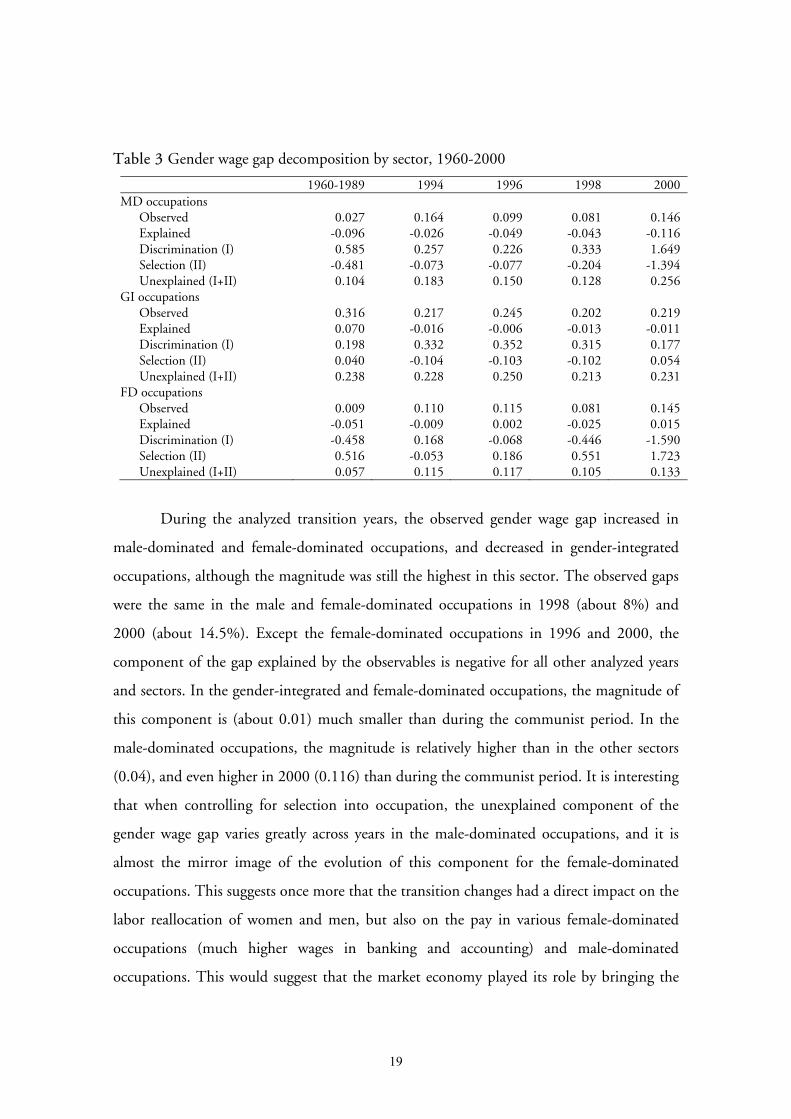
Table 3 presents the decomposition within each occupational sector, which for obvious

reasons does not include any occupational effect other then the effect that comes from self

18

selection. The wage differential between male and female was different across sectors, with

the highest observed differences in the gender-integrated occupations during all analyzed

years. In this sector, the observed gender wage gap was highest during the communist

regime, while the observed wage gaps for the other two sectors were almost zero: 2.7% in

the male-dominated occupations, and 0.1% in the female-dominated occupations. These

numbers are in accordance with the official policy of gender equality during the communist

regime, when wages were set according to industry-specific wage grids varying only with the

difficulty of the job and with worker education and experience, and not with gender.

Compared to other sectors, the female-dominated occupations were characterized by less

difficulty of the job tasks and less risk for accidents, which implies less “bonus”. These

occupations were also more homogenous with respect to requirements for education (for

example, the nurses and the teachers for the first four grades had graduated from specialized

high schools), which also implies relatively lower wages. On the contrary, almost all male-

dominated occupations were characterized by some degree of difficulty, which increased the

average wages. Moreover, it may have happened that women who worked in that sector

chose occupations with lower degree of difficulty, and therefore their average wages were

lower. The gender-integrated occupations may have included a diversity of occupations that

could be rewarded differently because of the different degrees of difficulty and various levels

of education. The selection into these occupations may explain the gender wage gap.

However, the endowments, or the part of the gender wage gap explained by the

observables, offer another picture of the gender gap. The explained part is negative and

much higher in magnitude than the observed gender wage gap in both male-dominated and

female-dominated occupations. This indicates women’s returns to endowments were

higher than those of their male peers. This was not the case for the gender-integrated

occupations, where the observables explain about 26% of the gender wage gap.

19

Table 3 Gender wage gap decomposition by sector, 1960-2000

1960-1989 1994 1996 1998 2000 MD occupations

Observed 0.027 0.164 0.099 0.081 0.146 Explained -0.096 -0.026 -0.049 -0.043 -0.116 Discrimination (I) 0.585 0.257 0.226 0.333 1.649 Selection (II) -0.481 -0.073 -0.077 -0.204 -1.394 Unexplained (I+II) 0.104 0.183 0.150 0.128 0.256

GI occupations Observed 0.316 0.217 0.245 0.202 0.219 Explained 0.070 -0.016 -0.006 -0.013 -0.011 Discrimination (I) 0.198 0.332 0.352 0.315 0.177 Selection (II) 0.040 -0.104 -0.103 -0.102 0.054 Unexplained (I+II) 0.238 0.228 0.250 0.213 0.231

FD occupations Observed 0.009 0.110 0.115 0.081 0.145 Explained -0.051 -0.009 0.002 -0.025 0.015 Discrimination (I) -0.458 0.168 -0.068 -0.446 -1.590 Selection (II) 0.516 -0.053 0.186 0.551 1.723 Unexplained (I+II) 0.057 0.115 0.117 0.105 0.133

During the analyzed transition years, the observed gender wage gap increased in

male-dominated and female-dominated occupations, and decreased in gender-integrated

occupations, although the magnitude was still the highest in this sector. The observed gaps

were the same in the male and female-dominated occupations in 1998 (about 8%) and

2000 (about 14.5%). Except the female-dominated occupations in 1996 and 2000, the

component of the gap explained by the observables is negative for all other analyzed years

and sectors. In the gender-integrated and female-dominated occupations, the magnitude of

this component is (about 0.01) much smaller than during the communist period. In the

male-dominated occupations, the magnitude is relatively higher than in the other sectors

(0.04), and even higher in 2000 (0.116) than during the communist period. It is interesting

that when controlling for selection into occupation, the unexplained component of the

gender wage gap varies greatly across years in the male-dominated occupations, and it is

almost the mirror image of the evolution of this component for the female-dominated

occupations. This suggests once more that the transition changes had a direct impact on the

labor reallocation of women and men, but also on the pay in various female-dominated

occupations (much higher wages in banking and accounting) and male-dominated

occupations. This would suggest that the market economy played its role by bringing the

20

wages to different levels, and policies such as affirmative action would have only limited

effect on the level of the unexplained wage gap. Nevertheless, the discrimination

component of the wage gap is negative for female-dominated occupations during

communist era and the last transition years (1996, 1998, and 2000), while positive and

relatively high in all other sectors during all analyzed years. This might suggest that women

working in female-dominated occupations were rewarded better than their peers men in

1996, 1998 and 2000, everything else being the same.

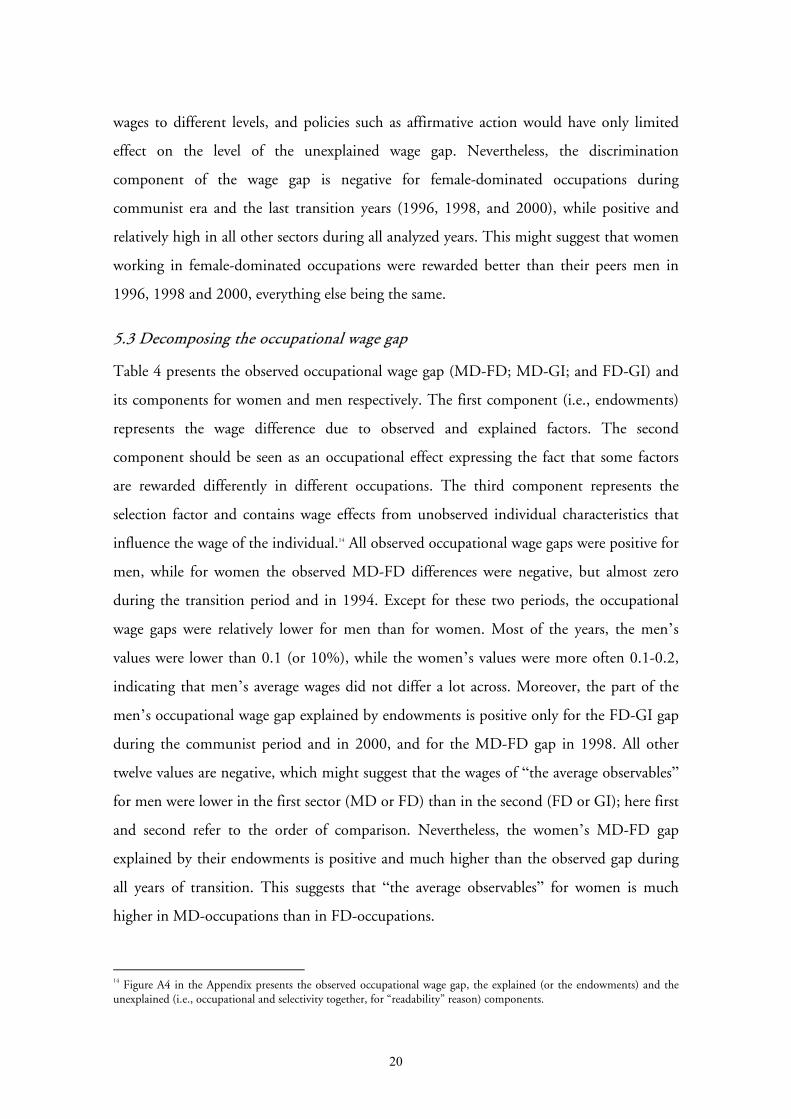
5.3 Decomposing the occupational wage gap

Table 4 presents the observed occupational wage gap (MD-FD; MD-GI; and FD-GI) and

its components for women and men respectively. The first component (i.e., endowments)

represents the wage difference due to observed and explained factors. The second

component should be seen as an occupational effect expressing the fact that some factors

are rewarded differently in different occupations. The third component represents the

selection factor and contains wage effects from unobserved individual characteristics that

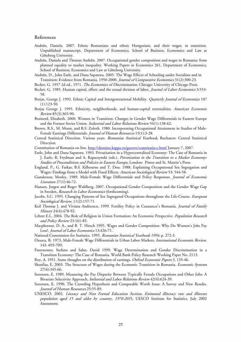
influence the wage of the individual.14 All observed occupational wage gaps were positive for

men, while for women the observed MD-FD differences were negative, but almost zero

during the transition period and in 1994. Except for these two periods, the occupational

wage gaps were relatively lower for men than for women. Most of the years, the men’s

values were lower than 0.1 (or 10%), while the women’s values were more often 0.1-0.2,

indicating that men’s average wages did not differ a lot across. Moreover, the part of the

men’s occupational wage gap explained by endowments is positive only for the FD-GI gap

during the communist period and in 2000, and for the MD-FD gap in 1998. All other

twelve values are negative, which might suggest that the wages of “the average observables”

for men were lower in the first sector (MD or FD) than in the second (FD or GI); here first

and second refer to the order of comparison. Nevertheless, the women’s MD-FD gap

explained by their endowments is positive and much higher than the observed gap during

all years of transition. This suggests that “the average observables” for women is much

higher in MD-occupations than in FD-occupations.

14 Figure A4 in the Appendix presents the observed occupational wage gap, the explained (or the endowments) and the unexplained (i.e., occupational and selectivity together, for “readability” reason) components.

21

Table 4 Occupational wage gap (owg) decomposition by gender

1960-89 1994 1996 1998 2000Women MD-FD owg Observed -0.003 -0.013 0.055 0.052 0.034E | , Endowments 0.113 0.077 0.112 0.116 0.168 Occupational (I) -1.302 -1.075 -1.018 -1.005 -1.185 Selectivity (II) 1.186 0.985 0.961 0.941 1.051 Unexplained (I+II) -0.116 -0.091 -0.057 -0.064 -0.134MD-GI owg Observed 0.415 0.120 0.203 0.200 0.199E | , Endowments 0.154 -0.015 0.006 -0.002 0.036 Occupational (I) -0.199 -0.316 -0.378 -0.490 -0.523 Selectivity (II) 0.460 0.451 0.575 0.692 0.687 Unexplained (I+II) 0.261 0.135 0.197 0.202 0.164FD-GI owg Observed 0.417 0.133 0.148 0.148 0.165E | , Endowments -0.004 -0.110 -0.112 -0.057 -0.029 Occupational (I) 1.147 0.778 0.646 0.453 0.560 Selectivity (II) -0.726 -0.534 -0.385 -0.248 -0.365 Unexplained (I+II) 0.421 0.244 0.260 0.205 0.195Men MD-FD owg Observed 0.015 0.040 0.039 0.053 0.034E | , Endowments -0.064 -0.026 -0.045 0.006 -0.085 Occupational (I) -0.128 -0.901 -0.617 -0.134 0.789 Selectivity (II) 0.207 0.967 0.700 0.181 -0.669 Unexplained (I+II) 0.079 0.067 0.083 0.046 0.180MD-GI owg Observed 0.126 0.067 0.057 0.079 0.126E | , Endowments -0.018 -0.040 -0.036 -0.025 -0.045 Occupational (I) 0.194 -0.377 -0.505 -0.481 0.163 Selectivity (II) -0.050 0.483 0.598 0.584 0.007 Unexplained (I+II) 0.144 0.106 0.093 0.104 0.214FD-GI owg Observed 0.110 0.026 0.019 0.026 0.091E | , Endowments 0.094 -0.050 -0.045 -0.089 -0.005 Occupational (I) 0.273 0.560 0.166 -0.288 -0.580 Selectivity (II) -0.257 -0.484 -0.102 0.404 0.676 Unexplained (I+II) 0.017 0.076 0.064 0.115 0.059

The unexplained portion of the wage gap is often interpreted as a result of

discrimination. Under this view, once differences among women in the relevant

determinants of wages are taken into account, any remaining difference in pay must be due

to discrimination. This cannot be gender discrimination, but something else that we cannot

observe. However, except for women’s MD-FD samples, for all other samples, the

unexplained part of the gap was positive and with a few exceptions, higher in magnitude

than the observed gaps. During the communist era, this might be a direct reflection of the

institutional settings of the labor market and the social security system, which gave

privileges (such as access to day care, health care subsidized lunches, etc.) only to workers

from given companies, while the variation in the unexplained part of the occupational wage

gap during the transition period could be due to a relative improvement in unmeasured

22

labor market skills. Nevertheless, the choice of occupation is related to the institutional and

democratic settings, and therefore the results are a reflection of the multitude of changes

accrued during the transition years. An individual who prefers characteristics associated

with a typical female occupation will be more likely to enter an FD occupation than

someone who prefers characteristics associated with a typical male occupation.

6 Summary and conclusions

After the communist regime’s fall in December 1989, Romania has experienced profound

political, democratic, and economic transformation. The labor market is one arena that

experienced most of the market economy shocks: the official birth of unemployment and

its social implications, the restructuring process of almost all big industrial companies and

the whole agricultural sector, the expansion of the private sector, the growth of a

decentralized system of wage setting, and the effect of these factors on the composition of

employment (who works and where). Ignoring the relatively large percentage of those who

did not work (many of them retired very early), our results show that the gender wage

differentials remained stable during the period, which may suggest that the structural

changes that occurred in 1994-2000 played a limited role in determining the gender wage

gap for those who worked. However, the reallocation of labor from the public to the private

sector (due mainly to the mass privatization of the state enterprises) was expected to

increase wage inequality and to result in a wider gender wage gap.

The very low values of the gender wage gap in female- and male-dominated

occupations support the hypothesis that if solidarity wage bargaining were effective in

promoting equal pay for equal job types, then controlling for job characteristics should

generate an adjusted pay gap of zero. In other words, this suggests some effects of the wage

bargaining in securing equal treatment of men and women in the Romanian labor market

during the communist regime.

The decomposition of the gender wage gap shows that the endowments (or the

observables) have a negative contribution to the overall difference. Moreover, during the

last analyzed transition years, the discrimination and the selection components of the wage

gap developed in opposite directions for male-dominated and female dominate

occupations. The discrimination component was negative only for the female-dominated

23

occupations, which might suggest that women working in the female-dominated

occupations were getting a “gender bonus”. Never the less, the “unadjusted” gender gap

might be explained (largely) by nondiscriminatory factors, such as family responsibilities

and especially the involvement of women and men in housework. However, given that the

economy and society in general and the labor market in particular experienced a multitude

of complex changes during the analyzed period, it is possible that much of the wage gap is

due to institutional norms, employer practices, and labor market policies. These three

elements changed continuously, and reflect the structural conditions of the labor market

and the societal restrictions, which may not only create different labor market opportunities

for different groups of people, but also relative values of different occupations in society.

The fact that women were less aggressive than men in the new free market economy created

an advantage for men, who become over-represented as managers and politicians at all

levels. There is also some anecdotal evidence that men use sexual harassment as a way to

reduce female competition in some segments of the labor market. Therefore, it is not

surprising that occupational differences explain a big part of the overall gender wage gap.

However, the macro statistics show that in the first years of the transition men were more

affected than women by the restructuring and closing of the big factories, and therefore it

could be that those who did not find job contributed to reducing the weight of the men

situated at the low end of the distribution of the offered wages. Even though the labor

participation of women and men was high during the communist era (exceeding 90%) and

even in the first years of transition (about 75%), the selection biases due to the fact that we

observe only the wages of persons who work might be a relatively high source of errors in

the assessment of wage differentials between groups and in the evaluation of the

components of these differentials.

Nevertheless, our results indicate that the wage differences were in general much

higher among workers of the same gender working in different occupations than between

women and men working in the same occupational group, and women experienced a larger

variation of occupational wage differentials than men during both regimes. These results

seem to be in line with earlier literature that support the belief that gender differences in

preferences play some role in gender differences in occupations (Gunderson, 1989).The

role of occupational upgrading in narrowing the gender pay gap raises the question of why

24

occupational differences between men and women have declined. The rise in women’s

acquisition of career-oriented formal education may reflect not only changes in women’s

preferences and their response to greater market opportunities, but also changes in the

admission practices of educational institutions and responses of other institutions that

support the promotion of women in a male-dominated world. In Romania, these factors

were strong during the communist period, but light, almost absent (in a broad perspective)

during the first years of transition, and this might contributed to the fact that the gender

wage gap was low during the communist regime, and higher during the transition years.

This implies that if policy makers are concerned with these issues, they should help women

more in gaining a career-oriented formal education. Additionally, women should be giving

assistance in motivating them to participate in the labor market in general, but also to

choose occupations that match their education.

Romania has no sustained debate about “making work pay”, instead in the

preparation for a European Union (EU) membership the focus has been on preparing the

legal and institutional processes and developing economic and social policy in line with EU

guidelines and requirements. However, the EU has an explicit commitment to raising the

employment rate for women and to advance gender mainstreaming and gender equality in

both employment and social inclusion policies. Moreover, even the measure of the gender

pay gap is part of the EU list of “structural indicators” (designed, after the Lisbon Special

European Council in March 2000, to follow up on progress regarding employment and

other issues). It seems that Romania would once more benefit from written and spoken

policies about women’s rights and their involvement in the labor market. We hope that

more would be invested in motivating Romanian women to get involved in well-paid

occupations, and girls and young women to acquire career-oriented formal education.

Additionally, more support should be given to all organizations that support women’s

promotion in the Romanian male-dominated society.

25

References

Andrén, Daniela. 2007. Ethnic Romanians and ethnic Hungarians, and their wages, in transition. Unpublished manuscript. Department of Economics, School of Business, Economics and Law at Göteborg University.

Andrén, Daniela and Thomas Andrén. 2007. Occupational gender composition and wages in Romania: from planned equality to market inequality. Working Papers in Economics 261, Department of Economics, School of Business, Economics and Law at Göteborg University.

Andrén, D., John Earle, and Dana Sapatoru. 2005. The Wage Effects of Schooling under Socialism and in Transition: Evidence from Romania, 1950-2000. Journal of Comparative Economics 31(2):300-23.

Becker, G. 1957 2d ed., 1971. The Economics of Discrimination. Chicago: University of Chicago Press. Becker, G. 1985. Human capital, effort, and the sexual division of labor, Journal of Labor Economics 3:553-

58. Borjas, George J. 1992. Ethnic Capital and Intergenerational Mobility. Quarterly Journal of Economics 107

(1):123-50. Borjas George J. 1995. Ethnicity, neighborhoods, and human-capital externalities. American Economic

Review 85(3):365-90. Brainerd, Elizabeth. 2000. Women in Transition: Changes in Gender Wage Differentials in Eastern Europe

and the Former Soviet Union. Industrial and Labor Relations Review 54(1):138-62. Brown, R.S., M. Moon, and B.S. Zoloth. 1980. Incorporating Occupational Attainment in Studies of Male-

Female Earnings Differentials. Journal of Human Resources 15(1):3-28. Central Statistical Direction. Various years. Romanian Statistical Yearbook, Bucharest: Central Statistical

Direction. Constitution of Romania on line. http://domino.kappa.ro/guvern/constitutia-e.html January 7, 2007. Earle, John and Dana Sapatoru. 1993. Privatization in a Hypercentralized Economy: The Case of Romania in

J. Earle, R. Frydman and A. Rapaczynski (eds.). Privatization in the Transition to a Market Economy: Studies of Preconditions and Policies in Eastern Europe, London: Pinter and St. Martin’s Press.

England, P., G. Farkas, B.S. Kilbourne and T. Dou. 1988. Explaining Occupational Sex Segregation and Wages: Findings from a Model with Fixed Effects. American Sociological Review 53: 544-58.

Gunderson, Morley. 1989. Male-Female Wage Differentials and Policy Responses. Journal of Economic Literature 27(1):46-72.

Hansen, Jorgen and Roger Wahlberg. 2007. Occupational Gender Composition and the Gender Wage Gap in Sweden, Research in Labor Economics (forthcoming).

Jacobs, S.C. 1995. Changing Patterns of Sex Segregated Occupations throughout the Life-Course. European Sociological Review, 11(2):157-71.

Keil Thomas J. and Viviana Andreescu. 1999. Fertility Policy in Ceausescu’s Romania. Journal of Family History 24(4):478-92.

Lehrer E.L. 2004. The Role of Religion in Union Formation: An Economic Perspective. Population Research and Policy Review 23:161-85.

Macpherson, D. A., and B. T. Hirsch 1995. Wages and Gender Composition: Why Do Women's Jobs Pay Less?. Journal of Labor Economics 13:426-71.

National Commission for Statistics. 1995. Romanian Statistical Yearbook 1994, p. 272-3. Oaxaca, R. 1973. Male-Female Wage Differentials in Urban Labor Markets, International Economic Review,

143. 693-709. Paternostro, Stefano and Sahn, David 1999. Wage Determination and Gender Discrimination in a

Transition Economy: The Case of Romania. World Bank Policy Research Working Paper No. 2113. Roy, A. 1951. Some thoughts on the distribution of earnings. Oxford Economic Papers 3, 135-46. Skoufias, E. 2003. The Structure of Wages during the Economic Transition in Romania. Economic Systems

27(4):345-66. Sorensen, E. 1989. Measuring the Pay Disparity Between Typically Female Occupations and Other Jobs: A

Bivariate Selectivity Approach, Industrial and Labor Relations Review 42(4):624-39. Sorensen, E. 1990. The Crowding Hypothesis and Comparable Worth Issue: A Survey and New Results.

Journal of Human Resources 25:55-89. UNESCO. 2002. Literacy and Non Formal Education Section, Estimated illiteracy rate and illiterate

population aged 15 and older by country, 1970-2015, UESCO Institute for Statistics, July 2002 Assessment.

26

UNESCO. 2005. Statistics in brief, Romania. UESCO Institute for Statistics. United Nations. 2003. Consideration of reports submitted by States parties under article 18 of the

Convention on the Elimination of All Forms of Discrimination against Women. Sixth periodic report of States parties. Romania, Committee on the Elimination of Discrimination against Women, CEDAW/C/ROM/6.

Vasile, Valentina. 2004. Gender equality issues examined. European industrial relations observatory on-line, http://www.eurofound.europa.eu/eiro/2003/12/feature/ro0312102f.html.

Vese, Vasile 2001. The condition of women in Romania during the communist period, in Ann Katherine Isaacs, ed., Political Systems and Definitions of Gender Roles, Edizioni Plus, Università di Pisa, 268.

27

Appendix

Figure A1 The women’s monthly net wages relative to men’s (in %)

a) Men

b) Women

Figure A2 The relative monthly net wages between occupations ( in %) by gender

70

100

130

1966-79 1971-75 1976-80 1981-85 1986-89 1990-93 1994 1995 1996 1997 1998 1999 2000

Male dominated Gender integrated Female dominated All occupations

60

100

140

1966-79 1971-75 1976-80 1981-85 1986-89 1990-93 1994 1995 1996 1997 1998 1999 2000

MD vs. FD MD vs. GI FD vs. GI

60

100

140

1966-79 1971-75 1976-80 1981-85 1986-89 1990-93 1994 1995 1996 1997 1998 1999 2000

MD vs. FD MD vs. GI FD vs. GI

28

Figure A3 The distribution of the occupational groups, 1960-2000, selected years

7.219.1

9.7

26.0

8.4

22.8

6.8

22.2

6.6

21.2

84.9

78.2

76.2

71.3

78.2

74.3

81.0

75.4

80.0

75.6

7.9 2.714.1

2.813.3

2.812.2

2.313.4

3.2

0

20

40

60

80

100

women men women men women men women men women men

1960-1989 1994 1996 1998 2000

(% ) Male dominated Integrated Female-dominated

29

a) MD-FD sectors differences

b) MD-GI sectors differences

c) FD-GI sectors differences

Figure A4 Occupational wage gap by gender, 1960-2000

E[Y(1)-Y(2)|X,Z]

-0.5

-0.4

-0.3

-0.2

-0.1

0.0

0.1

0.2

0.3

0.4

0.5

1960-89 1994 1996 1998 2000 1960-89 1994 1996 1998 2000

Men Women

Observed Explained Unexplained

E[Y(3)-Y(2)|X,Z]

-0.5

-0.4

-0.3

-0.2

-0.1

0.0

0.1

0.2

0.3

0.4

0.5

1960-89 1994 1996 1998 2000 1960-89 1994 1996 1998 2000

Men Women


E[Y(1)-Y(3)|X,Z]

-0.5

-0.4

-0.3

-0.2

-0.1

0.0

0.1

0.2

0.3

0.4

0.5

1960-89 1994 1996 1998 2000 1960-89 1994 1996 1998 2000

Men Women


30

Table A1 The public opinion about Who should be employed in the following domains

Domain Men Women Gender is not important Agriculture 0.22 0.02 0.76 Mining and metallurgy 0.87 0 0.13 Textile industry 0.03 0.74 0.23 Construction 0.83 0 0.17 Transportation 0.64 0 0.37 Education 0.03 0.25 0.72 Health 0.03 0.21 0.76 Public administration 0.17 0.07 0.76 Non-Governmental organizations 0.12 0.10 0.77 Media 0.06 0.06 0.88 Food Industry/Commerce 0.03 0.25 0.72 Banking System 0.16 0.09 0.75 Justice 0.28 0.04 0.69 Government 0.42 0.02 0.56

Table A2 Occupational concentration, 1966-2000

Proportion (%) of women working in

occupation with Proportion (%) of men working in

occupation with 50% + 55% + 60% + 65% + 70% + 75% + 50% + 55% + 60% + 65% + 70% + 75% + women workers men workers 1966-70 1231 25.8 25.8 25.8 5.0 0.0 0.0 74.2 55.6 55.6 47.4 14.5 14.51971-75 1312 43.2 21.8 15.0 15.0 9.2 9.2 56.8 56.8 56.8 14.8 11.8 11.81976-80 1683 37.1 21.1 14.3 14.3 14.3 4.9 62.9 57.2 16.0 16.0 1.8 0.31981-85 1740 32.9 15.6 15.6 6.0 6.0 0.0 67.1 67.1 20.2 14.2 14.2 2.11986-89 2361 14.7 14.6 14.6 14.6 5.3 5.3 85.4 54.4 12.2 12.2 12.2 1.5 1994 25549 27.0 16.3 16.3 16.3 7.5 7.5 73.0 54.1 54.1 54.1 19.2 17.41995 23644 28.3 28.3 17.2 17.2 7.7 7.7 71.7 53.3 53.3 53.3 53.3 17.81996 23910 37.9 28.2 17.1 17.1 7.3 7.3 62.1 53.7 53.7 53.7 16.7 14.01997 15502 37.8 28.6 16.7 16.7 7.0 7.0 62.2 53.2 53.2 53.2 16.3 14.81998 21515 49.0 29.7 17.3 17.3 6.7 6.7 51.0 51.0 51.0 51.0 15.4 13.21999 18961 50.8 31.3 18.8 18.8 7.5 7.5 49.2 49.2 49.2 49.2 14.9 13.62000 17480 40.8 31.9 19.5 19.5 7.8 7.8 59.2 48.9 48.9 48.9 14.6 13.4

31

Table A3 Descriptive statistics, male-dominated occupations,

1960-89 1994 1996 1998 2000

Men Women Men Women Men Women Men Women Men WomenWage# 1.472 1463.18 151.78 128.89 328.86 297.55 992.60 907.56 2348.77 2073.2Age 27.69 25.0 39.27 37.60 39.11 37.97 39.68 38.80 39.60 39.06Education

Lower education 0.76 0.66 0.67 0.56 0.66 0.53 0.65 0.49 0.61 0.48Medium education 0.17 0.29 0.26 0.38 0.26 0.39 0.26 0.42 0.30 0.43Higher education 0.06 0.04 0.07 0.06 0.08 0.08 0.08 0.08 0.09 0.09

Region R1: North-East 0.20 0.18 0.14 0.14 0.14 0.13 0.13 0.13 0.13 0.16R2: South-East 0.17 0.15 0.15 0.13 0.16 0.14 0.16 0.16 0.15 0.15R3: South 0.18 0.16 0.18 0.20 0.17 0.16 0.18 0.20 0.17 0.15R4: South-West 0.09 0.09 0.12 0.10 0.11 0.10 0.11 0.11 0.11 0.10R5: West 0.09 0.12 0.11 0.08 0.11 0.08 0.10 0.07 0.10 0.09R6: North-West 0.12 0.13 0.12 0.12 0.13 0.15 0.11 0.10 0.14 0.12R7: Center 0.09 0.10 0.11 0.11 0.10 0.11 0.12 0.12 0.11 0.10R9: Bucharest 0.06 0.08 0.08 0.12 0.08 0.12 0.09 0.12 0.10 0.13

Married 0.84 0.78 0.83 0.80 0.82 0.79 0.84 0.80 0.82 0.79Urban 0.51 0.72 0.55 0.74 0.54 0.74 0.57 0.78 0.63 0.82Ethnicity

Romanian 0.92 0.93 0.94 0.95 0.94 0.94 0.94 0.95 0.94 0.94Hungarian 0.06 0.06 0.05 0.04 0.05 0.05 0.05 0.04 0.05 0.05Other 0.02 0.01 0.01 0.01 0.01 0.01 0.01 0.00 0.01 0.01

Sector Agriculture 0.21 0.12 0.19 0.11 0.15 0.10 0.12 0.06Industry 0.36 0.74 0.32 0.67 0.32 0.68 0.32 0.69Services 0.42 0.14 0.49 0.22 0.53 0.22 0.55 0.25

Ownership State 0.83 0.88 0.89 0.92 0.80 0.80 0.67 0.65 0.48 0.36Private 0.09 0.05 0.08 0.05 0.14 0.13 0.23 0.20 0.37 0.47Other 0.06 0.04 0.01 0.02 0.00 0.02 0.00 0.01 0.00 0.01

Household members 3.56 3.57 3.95 3.74 3.84 3.68 3.76 3.62 3.64 3.42Multi-generation household 0.12 0.12 0.21 0.14 0.21 0.15 0.21 0.15 0.20 0.13Children <18 0.88 1.04 1.20 1.14 1.10 1.07 0.99 0.99 0.95 0.88n 1190 351 3887 1025 3137 860 2680 643 2025 521 Note: # monthly wage in thousands of Romanian lei, and it is the starting wage for 1951-1989. This holds for all tables.

32

Table A4 Descriptive statistics, gender-integrated occupations

1960-89 1994 1996 1998 2000








Household members 3.49 3.35 3.81 3.62 3.78 3.60 3.71 3.53 3.63 3.48Multi-generation household 0.13 0.08 0.22 0.16 0.24 0.19 0.24 0.19 0.24 0.20Children <18 0.84 0.87 1.13 1.06 1.05 0.98 0.96 0.87 0.87 0.81n 4934 4371 10671 8057 10202 7963 9097 7655 7224 6338

33

Table A5 Descriptive statistics, female-dominated occupations

1960-89 1994 1996 1998 2000








Household members 3.25 3.13 3.56 3.37 3.46 3.35 3.35 3.33 3.46 3.31Multi-generation household 0.12 0.12 0.20 0.16 0.20 0.18 0.20 0.17 0.20 0.16Children <18 0.63 0.67 0.90 0.83 0.87 0.78 0.75 0.75 0.78 0.72n 162 439 418 1491 391 1357 283 1157 309 1063

34

Table A6 Wage equation estimates by occupation, women, 1960-2000

1960-89 1994 1996 1998 2000Male-dominated Intercept 5.783 *** 3.685 *** 3.925 *** 4.541 *** 5.102 *** Age 0.034 0.114 0.593 *** 0.480 *** 0.419 * Age2/10 -0.009 -0.013 -0.080 *** -0.054 ** -0.044 Medium education -0.144 -0.068 -0.114 ** -0.133 ** -0.093 Higher education 0.318 *** 0.522 *** 0.527 *** 0.511 *** 0.762 *** Married 0.049 0.015 -0.014 -0.027 -0.131 ** Urban 0.095 ** 0.069 ** 0.155 *** 0.048 0.036 Agriculture 0.265 *** -0.049 -0.024 -0.112 -0.142 Industry -0.032 0.085 0.146 *** 0.070 0.219 *** State ownership -0.032 0.046 0.064 * -0.007 -0.029 Long-term contract -0.001 0.275 *** 0.038 0.175 0.447 *** Multi-generation household 0.040 -0.107 ** -0.121 ** -0.121 ** -0.198 *** Household members 0.008 -0.017 -0.003 0.006 Integrated Intercept 5.213 *** 3.946 *** 4.451 *** 5.118 *** 6.134 *** Age 0.090 0.189 *** 0.255 *** 0.268 *** 0.179 *** Age2/10 -0.022 * -0.019 *** -0.026 *** -0.024 *** -0.012 * Medium education 0.001 0.024 * 0.029 ** 0.045 *** 0.021 Higher education 0.363 *** 0.479 *** 0.522 *** 0.522 *** 0.532 *** Married 0.019 0.001 0.010 0.007 -0.007Urban 0.267 *** 0.107 *** 0.130 *** 0.117 *** 0.095 ***

Agriculture -0.056 0.103 ** 0.088 ** 0.078 ** 0.106 **

Industry -0.116 * 0.067 0.036 0.100 *** 0.084 *

State ownership 0.000 0.043 -0.057 * -0.024Long-term contract 0.064 ** 0.221 *** 0.169 *** 0.164 ***

Multi-generation household

Household members -0.005 -0.015 *** -0.018 *** -0.016 *** -0.032 ***

Female-dominated

Intercept 6.911 *** 4.947 *** 5.359 *** 6.038 *** 6.577 *** Age 0.211 0.151 0.285 *** 0.285 ** 0.300 ** Age2/10 -0.026 -0.016 -0.030 ** -0.029 * -0.029 * Medium education -0.216 *** -0.135 *** -0.145 *** -0.070 * -0.020 Higher education 0.319 *** 0.207 *** 0.278 *** 0.212 *** 0.255 *** Married -0.069 -0.033 -0.069 ** -0.038 0.000 Urban 0.054 0.119 *** 0.114 *** 0.062 ** 0.076 ** Agriculture 0.121 ** 0.191 *** 0.262 *** 0.055 0.020 Industry 0.113 *** 0.246 *** 0.198 *** 0.127 *** 0.119 *** State ownership 0.001 0.005 -0.052 ** -0.008 -0.008 Long-term contract 0.025 0.082 0.092 -0.013 0.234 ** Multi-generation household 0.081 -0.089 ** -0.124 *** -0.074 * -0.044 Household members 0.013 0.003 -0.024 ** -0.015 Note: we also control for region (5 dummies), ownership (3 dummies), and “time” (5 dummies controlling for the five-year periods for the communist period, and 11 monthly dummies for the transition years). This note holds also for the next table.

35

Table A7 Wage equation estimates by occupation, men, 1960-2000 1960-89 1994 1996 1998 2000Male-dominated Intercept 6.264 *** 3.887 *** 4.126 *** 5.560 *** 7.054 *** Age 0.146 0.283 *** 0.404 *** 0.068 0.315 *** Age2/10 -0.016 -0.035 *** -0.049 *** -0.006 -0.033 *** Medium education 0.026 0.001 0.008 0.006 0.198 *** Higher education 0.357 *** 0.409 *** 0.409 *** 0.438 *** 0.829 *** Married -0.031 0.076 *** 0.116 *** 0.166 *** 0.048 Urban 0.072 *** 0.094 *** 0.141 *** 0.091 *** 0.127 *** Agriculture 0.060 * -0.118 *** -0.100 *** -0.104 *** -0.428 *** Industry 0.054 0.003 0.036 ** 0.050 *** 0.138 *** State ownership -0.058 0.028 0.078 *** 0.127 *** 0.107 *** Long-term contract 0.002 0.144 *** 0.128 *** 0.074 0.082 Multi-generation household -0.011 -0.073 *** -0.073 *** -0.091 *** -0.029 Household members -0.003 -0.010 * -0.015 ** -0.008 Integrated Intercept 5.702 *** 4.231 *** 4.762 *** 5.451 *** 5.993 *** Age 0.038 0.281 *** 0.310 *** 0.326 *** 0.314 *** Age2/10 -0.003 -0.034 *** -0.036 *** -0.037 *** -0.031 *** Medium education 0.059 *** -0.002 -0.004 0.025 ** 0.116 *** Higher education 0.285 *** 0.309 *** 0.347 *** 0.373 *** 0.466 *** Married 0.020 0.079 *** 0.083 *** 0.122 *** 0.088 *** Urban 0.165 *** 0.099 *** 0.120 *** 0.123 *** 0.117 *** Agriculture 0.376 *** -0.005 -0.007 -0.088 *** -0.199 *** Industry 0.081 *** 0.081 *** 0.130 *** 0.124 *** 0.134 *** State ownership -0.014 0.050 *** 0.069 *** 0.076 *** 0.062 *** Long-term contract 0.006 0.070 *** 0.159 *** 0.154 *** 0.157 *** Multi-generation household 0.002 -0.085 *** -0.096 *** -0.077 *** -0.109 *** Household members -0.011 *** -0.006 * -0.010 *** -0.002 Female-dominated

Intercept 5.417 *** 4.374 *** 4.731 *** 5.501 *** 5.909 *** Age 0.596 ** 0.462 *** 0.553 *** 0.387 -0.166 Age2/10 -0.068 * -0.055 *** -0.060 *** -0.044 0.027 Medium education 0.131 * -0.114 *** -0.119 ** -0.102 0.111 * Higher education 0.269 ** 0.121 0.087 0.282 ** 0.337 *** Married -0.111 0.080 0.156 ** 0.014 0.161 ** Urban 0.256 *** 0.187 *** 0.176 *** 0.043 0.083 Agriculture 0.043 0.184 ** -0.001 -0.096 -0.280 *** Industry -0.120 0.072 0.104 0.046 0.073 State ownership -0.159 0.050 -0.030 -0.026 0.099 ** Long-term contract 0.065 ** 0.170 -0.022 -0.013 -0.094 Multi-generation household -0.254 * -0.070 0.028 -0.170 ** 0.004 Household members -0.020 -0.039 ** -0.016 0.009

Documents

Gender and occupational wage gaps in Romania - DiVA …oru.diva-portal.org/smash/get/diva2:174727/FULLTEXT01.pdf · Gender and occupational wage gaps in Romania: ... the Communist