Embed Size (px)
Citation preview
Inter-Industry Gender Wage Gaps by Knowledge Intensity: Discrimination and Technology in Korea Beyza P. Ural Department of Economics, Syracuse University, Syracuse NY, 13244, USA. William C. Horrace * Center of Policy Research, 426 Eggers Hall, Syracuse University, Syracuse NY, 13244, USA. [email protected] Jin Hwa Jung Department of Agricultural Economics and Rural Development, Seoul National University, San 56-1 Sillimdong Kwanakgu, Seoul 151-742, Korea.
ABSTRACT
A new gender wage gap decomposition methodology is introduced that does not suffer from
identification problems caused by unobserved non-discriminatory wage structure. The
methodology is used to measure the relative size of Korean gender wage gaps from 1994 to
2000 across industries, differentiated by industrial knowledge intensity, where knowledge
intensity is the extent to which industries produce or employ high-technology products. Korea
represents an important case study, since it possesses one of the fastest growing knowledge-
intensive economies, among industrialized countries. Empirical results indicate that over this
period, discrimination (the unexplained portion of the gender wage gaps) in Korea was
statistically smaller in knowledge-intensive industries than in industries with low knowledge
intensity. Also, discrimination was declining on average over the period. This suggests that
continued growth in knowledge-intensive industries in Korea may lead to further declines in
the overall gender gap.
JEL Codes: C12, J31, J71 Keywords: discrimination, labor markets, wage differential, compensation.
Running Title: Inter-Industry Gender Wage Gaps by Knowledge Intensity
* Corresponding Author

2
I. INTRODUCTION
Although there is an extensive body of literature on the decomposition of gender wage
differentials, based on a single cross-section of data, there have been relatively few studies that
analyze how these components evolve over time. For example, see Blau and Kahn (1999),
Kidd and Shannon (2001), or Finnie and Wannell (2004). In the last few years, many
developing countries have undergone substantial changes in their industrial compositions and
market structures, due to development strategies, shifting trade policies, and sectoral shifts in
the global economy (Freeman, 2004). Therefore, a dynamic analysis of the evolution of the
gender wage gap in a developing country seems particularly relevant. In particular, developing
countries in Asia experienced a substantial shift towards knowledge-intensive industries at the
end of the last decade (OECD, 2000), where knowledge intensity is measured as the extent to
which industries utilize a skilled or educated workforce or the extent to which technologically
advanced processes are used in the production of output.
An interesting question is then, "are these 'knowledge-based' industries more or less
prone to gender discrimination than "non-knowledge-based" industries?" A second interesting
question is, "to what extent has this shift towards knowledge-based industries been
accompanied with a change in the prevalence of gender discrimination in Asian economies?"
In this study, we analyze inter-industry gender wage gaps by knowledge intensity in Korea,
using a cross sectional occupational wage survey between the years 1994 and 2000. The
Korean economy provides a good test case, as the transition towards knowledge-based
industries in this country was substantial (OECD, 2000). Also, Korea experienced a steady
decrease in the overall female-male wage differentials.1 We find that in each year considered,
Korean knowledge-based industries were less discriminatory than non-knowledge-based
1 For non-agricultural industries, the average female-to-male earnings ratio was 44.2% in 1980 but was 63.2% in 2000 (Korean Labor Institute, Labor Statistics, 2004).

3
industries in terms of pay differentials. We also find that the decrease in the overall wage gap
was accompanied by a decrease in the discriminatory (unexplained) portion of the gap.
To analyze inter-industry wage differentials by knowledge intensity, we identify a new
decomposition methodology that allows us to make relative comparisons across industries and
across time. Conventional decomposition techniques (Oaxaca 1972, and Blinder, 1973) are not
identified in the sense that the investigator must decide a priori on an appropriate measure of
the unobserved non-discriminatory wage structure (Neumark, 1988). Our method identifies
relative inter-industry gender wage gaps and does not require an ad hoc proxy for the non-
discriminatory wage structure, because the estimation is designed to eliminate this structure,
when it can be assumed to be fixed across industries and across time. Our estimates reveal that
gender discrimination in knowledge-based industries was significantly lower than in non-
knowledge-based industries in Korea in all years considered. The results hold for knowledge-
based industries within both the manufacturing and service sectors of the Korean economy, as
well as for the economy as a whole. Our analysis reveals that dynamic fluctuations of
discrimination in the manufacturing sector at the end of the millennium were consistent with
the timing of the Asian financial crisis, and it may be possible that gender discrimination
improved during a period of intense industrial competition. While this is not formally
investigated or tested, it is consistent with the arguments of Becker (1971).
The paper is organized as follows. The next section summarizes theories that link
industrial composition and knowledge intensity to the magnitude of the unexplained gender
wage gap. In Section III, we develop a relative estimation strategy to estimate inter-industry
"non-discriminatory percentages", our normalized measure of gender discrimination. Our
strategy does not suffer from the lack of identification described by Neumark (1988). Section
IV describes the survey data used in this study, as well as the classification of industries into
"knowledge-based" and "non-knowledge-based" categories. Section V presents the empirical

4
results and compares the components of inter-industry wage differentials in knowledge-based
industries with non-knowledge-based industries. We repeat the analysis at a more
disaggregated level and compare the manufacturing sector and service sector by their
knowledge intensity. The final section summarizes and concludes.
II. INDUSTRIAL COMPOSITION AND GENDER WAGE GAPS
Krueger and Summers (1988) refueled an empirical and theoretical debate about the causes of
gender wage differentials. They found that the structure of the wage in the United States was
not compatible with a neoclassical model (Edin and Zetteberg, 1992), showing that inter-
industry gender wage disparities persisted between workers with identical individual
characteristics and working conditions. Several other studies, using standard wage regressions,
also support the existence of inter-industry gender wage differentials for apparently equally
skilled workers; many of these studies conclude that gender discrimination cannot be refuted.
See Gibbons and Katz (1992), Helwege (1992), Fields and Wolff (1995), and Abowd,
Karamarz, Margolis (1999).2 In the last decade, many developing countries experienced
changes in industrial composition due to development strategies, trade liberalization, and
global economic shifts (OECD, 2000). If the level of gender discrimination is different (lower)
in industries that are experiencing higher growth rates relative to other industries, then a
change (decrease) in the economies overall gender gap may accompany these changes in the
industrial composition (ceteris paribus).
There are several reasons why we might expect different levels of gender
discrimination in different industries. First, productivity of labor in some industries is an
increasing function of physical power for which the female labor force has comparative and
2 It is not our intent to argue the validity of wage regression for decomposing wage differentials, because they clearly have their drawbacks. However, they have been and continue to be a fairly standard tool in the literature.

5
absolute disadvantage. Other things being equal, it is natural to expect higher gender wage
disparities in these industries relative to the industries that do not require physical strength.
Clearly, this is an argument for a marginal product differential, but these differences may push
employers in these industries towards discriminatory tastes. Second, there are substantial
differences in the degree of competition in different industries due to differences in product
and labor markets, government regulations, and trade policies. Becker (1971) claims that
increasing competition results in lower levels of discrimination, which would cause inter-
industry differences in the wage gaps. Finally, given today's globalization of markets,
industries that are export-oriented (and not global monopolies) may be less likely to
discriminate in their long-run labor practices, as competition in international market precludes
survival of firms with inefficient (discriminatory) labor market practices.
Melitz (2003) develops a dynamic model to analyze the intra-industry effects of
international trade. In this model, exposure to trade causes only the most productive firms to
survive within an industry. There is also a large empirical literature showing that exposure to
trade increases the overall level of productivity in an industry through the mechanism
described above. In the classic Becker (1971) model, a firm (employer) that has tastes for
discrimination will employ fewer than the profit maximizing number of female employees, and
consequently will achieve suboptimal profits. We expect that market mechanism would force
firms with tastes for discrimination to exit the market, causing the overall level of
discrimination to be lower in export-oriented industries relative to industries that trade
domestically. Hellerstein, Neumark, and Troske (2002) test whether competitive market forces
reduce or eliminate discrimination using plant level longitudinal data. They find a positive
relationship between firm-level profitability and the proportion of female labor force. They
also find evidence that among plants with high market power, those that employ a relatively
large female labor force are more profitable, whereas no such relationship exist for plants with

6
low market power. The results are consistent with the short-run implications of Becker’s
model of employer discrimination.
There is also a class of models that posit differential employment search costs as
support for the existence of employer discrimination. Black (1995) constructs a model that
supports employer discrimination when sequential search costs are considered. In this model,
prejudiced employers only hire majority workers, whereas unprejudiced employers hire both
majority and minority workers. Since job search costs are higher for minority workers, they
lower their reservation wage, creating a wage differential between majority and minority
workers. Black's model also predicts that as the fraction of unprejudiced firms increases, the
wage differential vanishes, because search cost are effectively reduced for minority workers.
Therefore, if discrimination is different (lower) on average in developed counties than in
developing countries (for a variety of reasons that will not be discussed here), then a shift
towards trade liberalization and a global economy would (change) decrease wage differentials
in developing economies on average (ceteris paribus).
If there are differences between industries in terms of discriminatory practices, then the
evolution of gender wage gaps may be partially correlated with the changes in the industrial
structure of the countries, holding worker characteristics constant. Insofar as knowledge-based
industries are less capital intensive and more human capital intensive, they may exhibit smaller
(physical) capital barriers to entry and higher potential long-run competition than non-
knowledge-based industries. Assuming the existence of discrimination, as an economy shifts
towards more knowledge-based and (potentially) more competitive industries, the overall level
of gender wage gaps should decrease even when male-female characteristics are unchanged.
In this study, we identify and estimate a decomposition of inter-industry gender wage gaps by
knowledge intensity in Korea, a country that experienced a large transition to knowledge-based

7
industries in the last three decades.3 Korea is also an extreme example of rapid improvement
in the overall gender wage gaps, although gender wage gaps in Korea are still larger than most
OECD countries. Figure 1 shows the evolution of female-to-male ratio of earnings between
1980 and 2000. For non-agricultural industries, the female-to-male earnings ratio in Korea had
increased monotonically and quickly, from 44.2% in 1980 and 63.7% in 1998, and leveled off
between 1998 and 2000. This continuous improvement in the earnings ratio is associated with
an improvement in discrimination (or the unexplained portion of the usual average wage gap).
Our results indicate that there appears to be a strong correlation between a transition towards
knowledge-based industries and a decrease in gender discrimination in Korea at the end of the
millennium.
III. DECOMPOSITION FRAMEWORK
The classic Oaxaca-Blinder wage decomposition attempts to quantify gender discrimination in
a highly stylized Becker (1971) model (See Oaxaca, 1973 or Blinder, 1973). This
decomposition hinges on perfectly competitive labor markets where workers with the same
skills earn the same wage everywhere. That is, there exists some non-discriminatory wage
structure vector, θ , that maps the demographic attributes (including education, age, and
experience) of a worker into a wage, regardless of industry, occupation, or human capital
investment.4 Empirical implementations posit that if worker i possess demographic
characteristic vector, ix , then the worker should be paid a non-discriminatory wage, θii xy = ,
where the wage is typically in logarithmic form. Then, gender discrimination can be
quantified, in part, as deviations of observed male and female wage structures from the
unobserved or hypothetical standard, θ .
3 For years from 1990 to 2000, for instance, the growth of real value-added of the Korean economy was mainly led by knowledge-based manufacturing, while employment growth mainly led by knowledge-based services. For details, see Jung and Choi (2006). 4 In what follows, we effectively assume that this non-discriminatory structure is constant over time, as well.

8
While much has been written on the estimation of the male and female wage structures
using regression, little has been written on the estimation of θ to which the estimated
structures are to be compared, in order to quantify discrimination. The Oaxaca-Blinder
procedure proceeds by substituting either the estimated male wage structure or the estimated
female wage structure for θ to calculate discrimination. According to Neumark (1988),
substituting the estimated male wage structure implies the additional assumption that males are
paid their marginal product, while substituting the estimated female wage structure implies that
females are paid their marginal product. The choice of which estimate to use for the
unobserved non-discriminatory structure, θ , has implications for the measurement of
discrimination. An extreme example of this range is Ferber and Greene (1982), where wage
discrimination for a sample of university professors was 2 percent, based on the male non-
discriminatory wage structure, and was 70 percent, based on the female non-discriminatory
wage structure. It is in this sense that these estimates are "not identified." Neumark suggests
an alternative estimator for θ based on a regression that pools male and female observations in
the sample. The technique presented here use differences in counterfactual wage estimates to
produce measures of relative discrimination that are no longer a function of θ , so the arbitrary
decision on which structure to choose is eliminated. It is in this sense that our estimates are
"identified." 5
The goals here are: a) to partition a Korean labor market data set by year and industry,
where industries can be categorized as either "knowledge-based" or "non-knowledge-based"
and b) to estimate gender wage gaps over time and industry type to determine if gender wage
gaps have been statistically declining over time, and if their decline is in anyway related to
5 In the context of a 'data descriptive' wage model, 'identification' is not identification is the strictest sense of the word. However, the arbitrary selection of non-discriminator wage structure suggests a lack of identification, albeit an unconventional one. It is also admitted that a single non-discriminatory wage structure across all varieties of industries may be somewhat farfetched, even in perfectly competitive labor markets. However, this assumption is implicit in the wage decomposition literature, when decompositions are based on wage regressions that pool workers across industries.

9
knowledge intensity. These estimates are calculated at various levels of aggregation in the
data. The next subsection details estimation strategies at each level of aggregation considered.
A. Estimation of wage gaps
Let Kk ,...,1= index industries at different levels of aggregation (e.g., knowledge-based and
non-knowledge-based, or hi-tech, medium hi-tech, medium lo-tech, and lo-tech
manufacturing). Let Tt ,...,1= index time in years. Consider the T×2 log-wage regressions.
ft
K
kftkftkftftft dxy εβθ ++= ∑
=2 (1)
mt
K
kmtkmtkmtmtmt dxy εβθ ++= ∑
=2
(2)
where fty and mty are tF - and tM -dimensional column vectors, respectively, representing the
log wage for female and males, respectively; ftx and mtx are )( gFt × and )( gM t × dimensional
matrices, respectively, of observable explanatory variables; ftθ and mtθ are g-dimensional
parameter vectors; ftkβ and mtkβ are scalar parameters; ftkd and mtkd are tF - and tM -
dimensional vectors (respectively) of observable dummy variables for industry; and ftε and
mtε are tF - and tM -dimensional error vectors, respectively, satisfying the usual set of
regression assumptions. Define the following averages:
ftFt
ft xF
xt
ι′=1 )1( g× and mtM
tmt x
Mx
tι′=
1 )1( g×
where tFι and
tMι are tF - and tM -dimensional column vectors of ones, respectively. These
are average demographic characteristics in each year for females and males, respectively.
Ordinary least squares yields KT ××2 predicted counterfactuals in each industry:
ftkftftftk xy βθ ˆˆˆ += , (3)
10
mtkmtmtmtk xy βθ ˆˆˆ += , (4)
where 0ˆˆ11 == mtft ββ .
These are counterfactuals in the sense that we use ftx average female characteristics in
year t for all industries (instead of average female characteristics in year t in industry k) to
calculate ftky . This produces the predicted wage that an average female in year t would make
if they were randomly placed in industry k. The procedure is similar for calculating mtky .
This difference is essentially how identification is achieved. Then, KT × decompositions of
counterfactual male-female wage differences are:
θθθθθββ )()}ˆ()ˆ()ˆˆ{(ˆˆ mtftmtmtftftmtkftkmtkftk xxxxyy −+−−−+−=− (5)
where θ is some unobserved, non-discriminatory wage structure; it is the marginal product of
labor of a labor market that does not have tastes for discrimination. This is similar to the
Oaxaca-Blinder decomposition with one minor difference: the counterfactual male-female
differential is decomposed and not the average male-female differential (say, mtft yy − ).
Using the counterfactual seems reasonable, because the Oaxaca-Blinder decomposition
implicitly assumes that labor markets are competitive, and in this highly stylized world, labor
should be readily substitutable across industries, particularly when it is the average laborer
being substituted. In what follows, we cannot solve or account for this particular shortcoming
of the model.6
A particularly appealing feature of this formulation of the decomposition is that
equation (5) highlights the fact that the explained portion of the gap, θ)( mtft xx − , is not
identified. Therefore, the extent to which changes in the overall gap over t due to changes in
average male-female characteristic differential, )( mtft xx − , is not estimable without knowing
6 That is, we still must assume that θ is constant over industries, and also over time.

11
θ . Therefore, even gender wage differences based on worker productivity differences are not
measurable in the context of the Oaxaca-Blinder decomposition. This is important, because the
decomposition is usually dichotomized into an "explained" and an "unexplained" portion, but
without knowledge of θ , nothing is truly "explained."
This may seem like a somewhat grim view of the Oaxaca-Blinder decomposition, but
the decomposition is salvageable (in some sense). The problem is that the decomposition seeks
to identify a dichotomy based on some "gold standard", θ , which assigns weights (or
importance) to average worker characteristics. However, if the gold standard is the same
across industries (as these models typically assume), then we can use the variability over k to
identify a relative measure of discrimination that is based on some male and female worker of
average characteristics working in any industry k and being paid some economy-wide gold
standard, θ . (This is the essence of the identifying assumption.) Based on equation (5),
discrimination (the bracketed potion of the counterfactual wage decomposition in the equation)
is:
)}ˆ()ˆ()ˆˆ{(),,(ˆ θθθθββθδ −−−+−= mtmtftftmtkftkmtfttk xxxx (6)
which is also not identified, since θ is not identified. Let ),,(ˆmax),,(ˆ][ mtfttkkmtftkt xxxx θδθδ = .
Notice that because of the linearity (monotonicity) of the decomposition, it doesn't matter what
we use for θ to find the index of the maximum, ][k . The magnitude of ),,(ˆ][ mtftkt xxθδ is a
function if θ , but the index of the maximum, ][k , is the same regardless of what is selected
forθ , because it is mapping into a set of characteristics, ftx or mx that doesn't vary over k.
Therefore, selecting 0=θ is fine for finding ][k , but mtθθ ˆ= is what is normally used (men
are paid the non-discriminatory standard, and women are paid below it). Then differencing
across k:
),,(ˆ),,(ˆ),(ˆ ][ mtfttkmtftktmtfttk xxxxxx θδθδγ −= (7)

12
)ˆˆ()ˆˆ(),(ˆ ][][ mtkftkkmtkftmtfttk xx ββββγ −−−= (8)
These are comparisons within years but between industries, and they sweep out the non-
discriminatory wage structure, θ , and are therefore identified. Relative estimators of this type
were first considered by Horrace and Oaxaca (2001). Horrace (2005) explains that these
measures are "relative to a within sample standard," and argues that the differencing may
reduce estimation biases associated with non-zero means for ftε and mtε .
The measure in (8) identifies relative comparisons between industries while sweeping
out θ but (unfortunately) not between years, because the averages ftx and mtx are a function
of t. To make comparisons between years and occupations, define the averages male and
female characteristics across industries and years as fx and mx . Let
∑=
=T
ttFF
1 and ∑
=
=T
ttMM
1
then grand means over all years and industries are
∑=
=T
tfttf xF
Fx
1
1 )1( g× and ∑=
=T
tmttm xM
Mx
1
1 )1( g×
Plugging these values in for ftx and mtx in the previous analysis, we can difference across k
and t. Let
)}ˆ()ˆ()ˆˆ{(),,(ˆ θθθθββθδ −−−+−= mtmftfmtkftkmftk xxxx (9)
Let ),,(ˆmax),,(ˆ,][ mftkktmftk xxxx θδθδ = , so that
),,(ˆ),,(ˆ),(ˆ ][ mftkmftkmftk xxxxxx θδθδγ −= (10)
and,
)ˆˆ()ˆˆ()ˆˆ()ˆˆ(),(ˆ ][][][][ mttmmfttffmtkftktkmtkfmftk xxxx θθθθββββγ −−−+−−−= , (11)

13
where ][tk corresponds to the index of the maximal tkδ for 0=θ over both k and t , and
where ][t corresponds to index of the same year associated with ][tk . These are comparisons
between years and industries, that sweep out θ , because the averages fx and mx are no longer
a function of t .
There is some industry in some year, ][tk , that possesses that maximal value of the
unexplained counterfactual wage gap (discrimination): ][tkδ . Then the difference, 0ˆ ≥tkγ ,
captures the (relative) extent to which industry k in year t is discriminatory. A convenient
normalization is the "non-discriminatory percentage" ]1,0(}~exp{ ∈− tkγ , Kk ,...,1= , Tt ,...,1= .
The normalization can be interpreted as follows: "in a labor market where skill and the non-
discriminatory wage structure are constant over industry and time (save for the differentials
ftkβ and mtkβ ), industry-year ][tk is 100 percent non-discriminatory relative to all industry-
years in the sample tk , and all other industry-years are some fraction (of 100 percent) non-
discriminatory." Clearly, certain problems inherent in the classical Oaxaca-Blinder
decomposition remain here. For example, actual labor markets are marked with some level of
heterogeneity across industries in terms of worker characteristics and (presumably) in terms of
their non-discriminatory wage structures. However, our measure does not suffer from the lack
of identification embodied in an arbitrary selection of, say mtθθ ˆ= . Also, there is truly no
sense in which we have identified the "unexplained portion" of some observed wage gap,
mtft yy − . In fact we are decomposing the estimate mtkftk yy ˆˆ − , which is technically "not
observed," so there is no way to relate our measure back to the overall gap, mtft yy − .
However, this is the cost of the identification: everything is relative to the unidentified
difference ),,(ˆ][ mftk xxθδ , not the "identified" difference mtft yy − .

14
The estimates in equation (11) are used in the empirical analyses that follow. First, we
partition the data into "knowledge-based industries" and "other industries", so that K = 2 (one
dummy variable in each regression). This produces two estimate of ),(ˆ mfkt xxγ in each of
seven years, 2000,...,1994=t . Then, we partition the data into four industries: knowledge-
based manufacturing, knowledge-based services, other manufacturing, and other services, so
that K = 4 (three dummy variables in each regression). This produces four estimates of
),(ˆ mfkt xxγ in each of seven years, 2000,...,1994=t . We now discuss variance estimation for
the estimates in equation (11).
B. Variance-covariance estimation
Since θ will ultimately be eliminated by differencing, we set 0=θ in what follows. Hence,
the estimator of interest is:
)ˆˆ()ˆˆ(),,0(ˆmtkmtmftkftfmftk xxxx βθβθδ +−+= (12)
Let ]ˆ,...,ˆ,ˆ[ˆ2
* ′= ftKftftft ββθθ and ]ˆ,...,ˆ,ˆ[ˆ2
* ′= mtKmtmtmt ββθθ be )1( −+ Kg column vectors, so
that ]ˆ,...,ˆ[ˆ **1
* ′= fTff θθθ and ]ˆ,...,ˆ[ˆ **1
* ′= mTmm θθθ are )1( −+ KgT column vectors. Let Q be a
1−K identity matrix bordered above by a 1−K row vector of zeros. Therefore Q is a
)1( −× KK matrix. Therefore, ],[ QxIC fKTf ⊗⊗= ι and ],[ QxIC mKTm ⊗⊗= ι are
)1( −+× KgTTK matrices. Then,
**
)1(
ˆˆ),,0(ˆmmff
TKmf CCxx θθ −=Δ
×
(13)
is a TK column vector, and is the vector representation of the estimates in equation (12), with
typical element tkδ . Let D be constructed from a ( 1)TK − negative identity matrix with a
column vector of ones inserted in ][tk column position from the left and then a column of

15
zeroes inserted in the ][tk row position from the top. For example if ][tk is the second element
of Δ , then
⎥⎥⎥⎥⎥⎥⎥⎥
⎦
⎤
⎢⎢⎢⎢⎢⎢⎢⎢
⎣
⎡
−
−−
−
=×
10010001010001100000000011
)(
L
OMMMM
L
L
L
L
TXTKD
Then,
),,0(ˆ)]',(ˆ)...,(ˆ[),(ˆ11
1mfmfTKmf
TKmf xxDxxxxxx Δ==Γ
×
γγ (14)
is the vector representation of the ),(ˆ mftk xxγ in equation (10). Since the male and female
samples are independent,
DCVarCCVarCDxxVar mmmfffTKTK
mf ′′+′=Γ×
])ˆ()ˆ([)},(ˆ{ ** θθ
(15)
Treating the samples in each of the T regressions as independent,
⎥⎥⎥⎥⎥
⎦
⎤
⎢⎢⎢⎢⎢
⎣
⎡
=
)ˆ(
)ˆ()ˆ(
)ˆ(
*
*2
*1
*
fT
f
f
f
Var
VarVar
Var
θ
θθ
θ
K
MOMM
K
K
00
0000
,
a )1( −+ KgT square matrix, where )ˆ( *ftVar θ is a )1( −+ Kg square matrix returned by any
regression software package. It follows similarly for )ˆ( *mtVar θ . Also notice that θ is a
constant, so it is true that
)},,0(ˆ{)},,(ˆ{)(
mfTKTK
mf xxVarxxVar Δ=Δ×
θ (16)
Therefore,

16
mmmfffmf CVarCCVarCxxVar ′+′=Δ )ˆ()ˆ()},,(ˆ{ ** θθθ (17)
IV. DATA
The data used for the empirical analysis are from the 1994 to 2000 Wage Structure Survey of
the Ministry of Labor of Korea, and were previously analyzed by Jung and Choi (2004, 2006).
The survey provides information on personal characteristics and earnings data for workers
employed in firms with 10 or more employees in all industries, except the public
administration sector.7 For the empirical analysis, the agricultural and mining industries, as
well as agricultural occupations, were excluded. The final data set includes about 0.4 million
workers for years 1994-1998, and about 0.5 million workers for 1999 and 2000.
The industrial classification for the empirical analysis is presented in Table 1.
Knowledge-based manufacturing sectors are classified based on their R&D intensity and
knowledge-based service sectors are classified based on the ratio of college graduates.
Knowledge-based manufacturing refers to high-technology manufacturing in areas such as
electronics and communication equipment, and also to medium-high-technology
manufacturing in areas such as computers and motor vehicles. Other manufacturing includes
medium-low-technology manufacturing covering chemicals, rubber and plastic products,
metals, and also low-technology manufacturing ranging from food and textiles to paper
products. Knowledge-based services include communications, finance, business services,
health, education, and cultural services. Non-knowledge-based services or "other services"
include the industries like utilities, construction, wholesale and retail trade, hotels and
restaurants, and transport and storage. These industrial groupings were made based upon the
two-digit Korean Standard Industrial Classification (KSIC). 7 The Survey was extended to include small firms with 5-9 employees starting in 1999, but workers employed in firms with 5-9 employees were excluded from the final data set for consistency.

17
V. RESULTS
In order to estimate non-discriminatory percentages for industry groups, wage regressions for
male and female groups were estimated for years 1994 to 2000. The first set of regressions
included dummy variables for whether an individual was employed in a knowledge-based
industry or not. Estimation results of these regressions are presented in Table 3. As an
estimator of equation (11), we report two values ( 2,1=k ; knowledge- and non-knowledge-
based) of the "non-discriminatory percentages," }ˆexp{ tkγ− , for seven years 7,...,1=t . The top
section of Table 5 contains these values and the standard errors of the estimators.8 Here, the
largest value of 4445.0ˆ][ −=tkδ corresponds to the knowledge-based industries in 1999.9
Thus, for knowledge-based industries in 1999, 0ˆ =tkγ and 1}ˆexp{ =− tkγ , so in 1999
knowledge-based industries were "100 percent non-discriminatory," meaning that, relatively
speaking, knowledge-based industries in 1999 were the least discriminatory industry-year in
the sample. All other industry-years are evaluated relative to this standard.
Table 5 shows that, in 1994 knowledge-based industries were 93.8 percent non-
discriminatory and non-knowledge-based industries were 90.7 percent non-discriminatory. In
2000, knowledge-based industries were 98.4 percent nondiscriminatory and non-knowledge-
based industries were 96.2 percent non-discriminatory. Figure 2 shows the values of non-
discriminatory percentages as well as 95 percent confidence intervals based on the standard
errors in equation (17). According to our estimation, knowledge-based industries had
significantly higher non-discriminatory percentages in all years considered. Although in 1996
8 Note that the standard errors are for tkγ not the normalization }ˆexp{ tkγ− , but they can be used to calculate
confidence intervals on the }ˆexp{ tkγ− , since it is a monotonic transformation of tkγ . We do this in the sequel. 9 Note that 4445.0ˆ
][ −=tkδ is not readily interpretable as a measure of discrimination, because it is evaluated at
0=θ .

18
the two estimates were relatively close, the difference was still significant based on the 95
percent confidence intervals. The non-discriminatory percentages in the two groups of
industries follow a different trend between 1994 and 2000. Non-knowledge-based industries or
"other industries" (the solid line) show a relatively fast improvement between 1994 and 1996,
followed by a relatively steady three years and a significant improvement in 2000. Knowledge-
based industries (the dashed line), however, follow a different pattern. Between 1994 and 1996
non-discrimination improved very slightly, followed by a large improvement in 1997 and an
insignificant decline in 1998. In 1999, knowledge-based industries have the largest non-
discriminatory percentage (100 percent), but it decreased to 98.4 percent in 2000.
There is a strong possibility that we are picking up the effects of the Asian Financial
Crisis that occurred between 1997 and 1998. This may be particularly true for knowledge-
based manufacturing industries in Korea, which experienced very strong growth immediately
before the financial crisis. The OECD (2000) report characterizes Asian economies before the
financial crisis as “industrial over-capacity due to excessive investment in manufacturing”.
The rapid increase in the non-discriminatory percentages for knowledge-based industries
between 1996 and 1997 may be correlated with this over-capitalization in Asian manufacturing
and the subsequent steep decline in Asian currencies after the crisis. It is not clear what
mechanism produced this apparent correlation, nor are we willing to speculate on it, since it is
beyond the scope of this research. However, the coincidence of the decrease in the
unexplained portion in the gender wage in Korean knowledge-based industries and the Asian
financial crisis is too pronounced in Figure 2 to be ignored. In the next analysis, we will show
that the changes in discrimination for knowledge-based industries were, in fact, substantial in
the manufacturing sector, but weak or non-existent in the service sector.
To disaggregate the industry effects, we re-estimated the regressions with three industry
dummies representing the knowledge-based manufacturing, knowledge-based services, non-

19
knowledge-based manufacturing (other manufacturing), and the non-knowledge-based services
(other services) as the omitted category. The regression results are tabulated in Table 4.
Normalized estimates of equation (11) can be found in Table 5. Figures 3 and 4 show the
evolution of non-discriminatory percentages for these four industry classifications. Lower and
upper limits of confidence intervals (based on standard errors reported in Table 5) show that
the non-discriminatory percentages were significantly higher in knowledge-based industries for
both manufacturing and services.
The empirical finding that non-discriminatory percentages are significantly higher in
knowledge-based industries is consistent with the hypothesis that non-productivity related
discrimination in knowledge-based industries is more costly than in non-knowledge-based
industries. That is, non-productivity related discrimination is perhaps more detrimental to the
competitiveness of knowledge-based industries than non-knowledge-based industries, where
the former is heavily dependent upon knowledge inputs, and perhaps subject to a higher degree
of competition. Notice, also, that non-discriminatory percentages are higher in services than in
manufacturing. Non-discriminatory percentages in non-knowledge-based services are lower
than those in knowledge-based services and are higher than those in both knowledge-based and
non-knowledge-based manufacturing. Also, the difference in non-discriminatory percentages
between knowledge-based sectors and non-knowledge-based sectors is smaller for
manufacturing than for services.
Again, there seems to be some (unexplained) correlation between the steep increases in
the non-discriminatory percentages in the manufacturing sector (Figure 4) and the Asian
Financial Crisis that occurred between 1997 and 1998. In Figure 4, we see a significant drop in
1999 knowledge-based manufacturing industries, as well as in non-knowledge-based
industries. Although it is beyond the scope of this paper to analyze effects of the Asian crisis
on Korean labor markets, it is interesting to see that the improvements in non-discriminatory

20
percentages between 1994 and 1998 were partially reversed in knowledge-based
manufacturing industries and completely reversed in non-knowledge-based manufacturing
industries as the financial crisis was mitigated. In 2000, there was a significant improvement in
non-knowledge-based industries and a slight decrease in knowledge-based industries. Figure 3
shows that, in the service sector, the correlation between the financial crisis and gender
discrimination was not as clear as in the manufacturing sector. In 1998, there was a slight
decrease in non-discriminatory percentages in non-knowledge-based services, followed by a
significant improvement. In knowledge-based service industries, however, there was a slight
decrease in the trend, followed by a significant improvement. In 2000, both knowledge- and
non-knowledge-based service industries experienced a decline in non-discriminatory
percentages.
VI. CONCLUSIONS
If one accepts the validity of Oaxaca-Blinder decompositions from linear wage regressions
then the counterfactual decomposition presented herein is identified, while the usual
decomposition is not. Our technique also readily lends itself to comparisons across separate
regression periods and to a convenient normalization of discrimination to percentages on the
unit interval. We have also provided an explanation of how to calculate standard errors for our
estimates. Our technique could be applied to any partition of the data (not just a partition
based on knowledge intensity) and to other forms of discrimination (e.g., discrimination by
race), as well.
Our application suggests that discrimination was smaller in knowledge-intensive
industries in Korea than in non-knowledge-intensive industries at the end of the last decade,
and this difference seems to have been most pronounced in the manufacturing sector. In
absolute terms we do not know the difference and by how much it changed over time; this is

21
the cost of the relative estimation procedure. There was some volatility in the level of
discrimination around the time of the Asian Financial Crisis, particularly in the manufacturing
sector. Despite this volatility, discrimination declined on average over the seven-year period.
It would be interesting to explore the nature of the causality (if any) between the overall
decline in discrimination and the events surrounding the Asian Financial crisis, but this is left
for future research.
ACKNOWLEDGEMENTS
We would like to thank to Dan Black, Tom Kniesner, Devashish Mitra, Joseph Marchand, and
participants in American Economic Association 2005 Meetings in Philadelphia for their helpful
comments. The authors are responsible for all remaining errors.

22
REFERENCES Abowd, J.M., Karamarz F., and Margolis D.N. (1999) High wage workers and high wage firms. Econometrica, 67, 251-333. Altonji J.J. and Blank, R.M. (1999) Race and gender in the labor market, in: O. Ashenfelter & D. Card (ed.), Handbook of Labor Economics, edition 1, volume 3, chapter 48, pages 3143-3259, Netherlands: Elsevier. Becker, G.S. (1971) The Economics of Discrimination, Chicago: University of Chicago Press. Black, D. (1995). Discrimination in an equilibrium search model. Journal of Labor Economics, 13, 308-33. Blau, F.D. and Kahn, L.M. (1999). Analyzing the gender pay gap. Quarterly Review of Economics and Finance, 39, 625-646. Blinder, A.S. (1973). Wage discrimination: reduced form and structural estimates. The Journal of Human Resources, 8, 436-455. Edin, P and Zetteberg, J. (1992) Interindustry wage differentials: evidence from Sweden and a comparison with United States. The American Economic Review, 82, 1341-1349. Ferber, M.A., and Green, C.A. (1982) Traditional or reverse sex discrimination? A case study of a large public university. Industrial and Labor Relations Review, 35, 550-64. Fields, J. and Wolff E. (1995) Interindustry wage differentials and gender wage gap. Industrial and Labor Relations Review, 49, 105-120. Finnie, R and Wannell T. (2004) Evolution of the gender earnings gap among canadian university graduates, Applied Economics 36, 1967-78. Freeman, R. (2004). The great doubling: the real effect of globalization on labor. Unpublished Manuscript, Department of Economics, Harvard University. Gibbons F. and Katz L. (1992) Does unmeasured explain inter-industry wage differentials? Review of Economic Studies, 59, 515-535. Hellerstein J.., Neumark, D. and Troske, K.R. (2002) Market forces and sex discrimination. Journal of Human Resources, 37, 353-380. Helwege, J. (1992) Sectoral shifts and inter-industry wage differentials, Journal of Labor Economics, 10, 55-84. Horrace, W.C. (2005) On the ranking uncertainty of labor market wage gaps. Journal of Population Economics, 18, 181-187. Horrace, W.C. and Oaxaca, R.L. (2001) Inter-Industry Wage differentials and the gender wage gap: an identification problem Industrial and Labor Relations Review, 54, 611-618.

23
Jung, J.H. and Choi K. (2004) Gender wage differentials and discrimination in Korea: comparison by knowledge intensity of industries, International Economic Journal, 18, 561-579. Jung, J. H. and Choi K. (2006) The labor market structure of knowledge-based industries: a Korean case. Journal of Asia Pacific Economy, 11, 59-78. Kidd, M.P. and Shannon M. (2001) Convergence in the gender wage gap in Australia over the 1980s: identifying the role of counteracting forces via the Juhn, Murphy and Pierce decomposition, Applied Economics 33, 929-36. Krueger B.A. and Summers L.H. (1988) Efficiency wages and inter-industry wage structure, Econometrica, 56, 259-293. Melitz, M.J. (2003) The impact of trade on intra-industry reallocations and aggregate industry productivity, Econometrica, 71, 1695-1725. Neumark, D. (1988) Employers’ discriminatory behavior and the estimation of wage discrimination. The Journal of Human Resources, 23, 279-295. Oaxaca, R., (1973) Male-female wage differentials in urban labor markets. International Economic Review, 14, 693-709. Oaxaca, R.L. and Ransom M. (1999) Identification in detailed wage decompositions., Review of Economics and Statistics, 81, 154-157. OECD (2000) Knowledge-based Industries in Asia. OECD. Paris.

24
FIGURES
Figure 1: Female-to-Male Ratio of Average Earnings
0.40
0.45
0.50
0.55
0.60
0.65
1980 1985 1990 1995 2000
Source: Korean Labor Institute, Labor Statistics (2004). Figure 2: Non-Discriminatory Percentages, Knowledge-based Industries and Other Industries
0.900
0.925
0.950
0.975
1.000
1994 1995 1996 1997 1998 1999 2000
Knowledge Based Industries Other Industries
Figure plots }ˆexp{ tkγ− where tkγ is based on equation (11). [tk] = [Knowledge-based Industries, 1999]. 95% confidence bounds. Other Industries = Non-Knowledge-based Industries.

25
Figure 3: Non-Discriminatory Percentages, Knowledge-based Services and Other Service
0.8000
0.8500
0.9000
0.9500
1.0000
1994 1995 1996 1997 1998 1999 2000
Know ledge Based Services Other Services
Figure plots }ˆexp{ tkγ− where tkγ is based on equation (11). [tk] = [Knowledge-based Services, 1999]. 95% confidence bounds. Other Services = Non-Knowledge-based Services.
Figure 4: Non-Discriminatory Percentages, Knowledge-based Manufacturing and Other Manufacturing
0.7500
0.7750
0.8000
0.8250
0.8500
1994 1995 1996 1997 1998 1999 2000
Know ledge Based Manufacturing Other Manufacturing
Figure plots }ˆexp{ tkγ− where tkγ is based on equation (11). [tk] = [Knowledge-based Services, 1999]. 95% confidence bounds. Other Manufacturing = Non-Knowledge-based Manufacturing.

26
Table 1: Classification of Knowledge-based Industries
R&D Intensity1
(1999)
College Graduates2
(2001) Knowledge- High-tech Electronical machinery 10.6 16.8 based Communication equipment 17.9 19.8 Manufacturing (KBM) Medium-high-tech Office/accounting/computing machinery 7.0 17.0
Motor vehicles 8.9 11.8 Other Medium-low- Chemicals 3.6 29.6 Manufacturing tech Rubber/plastic products 3.5 12.1 (OM) Non-metallic mineral products 1.9 11.5 Metals 1.0 13.6 Fabricated metal products 1.0 8.9 Non-electrical machinery 3.6 11.5 Precision instruments 4.1 8.9 Other transport equipment 1.1 26.5 Furniture, and Manufacturing n.e.c. 1.6 10.2 Low-tech Food, beverages, tobacco 0.7 10.0 Textiles, apparel, leather 0.9 6.7 Wood and paper products 0.5 3 14.1 Printing - 29.0 Petroleum refineries/products 0.5 44.7 Recycling - 3.8 Knowledge- Communications 5.0 29.2 based Financial services - 31.0 Services Business services - 35.2 (KBS) Education services - 59.5 Health services/social work - 31.2 Culture/recreation - 23.3 Other Electricity, gas, water supply 0.9 30.7 Services Construction 0.7 13.2 (OS) Wholesale/retail trade - 15.4 Hotels and restaurants - 4.7 Transport and storage - 10.9 Real estate activities - 15.0 Other services - 18.7
All Industries 1.8 19.0 Notes: 1) R&D expenditures as a percentage of value added in each industry. 2) The ratio of 4-year college graduates to the total employed(%). 3) Includes printing industry. Sources: OECD(2002), Science, Technology and Industry Outlook, NSO, Korea(2002), The Economically Active Population Survey.

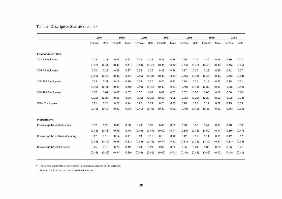
Table 2: Descriptive Statistics*
1994 1995 1996 1997 1998 1999 2000
Female Male Female Male Female Male Female Male Female Male Female Male Female Male
Logarithm of Hourly Wage (Won) * 8.00 8.55 8.16 8.68 8.34 8.84 8.44 8.92 8.45 8.93 8.46 8.90 8.59 9.02
(0.44) (0.49) (0.45) (0.49) (0.46) (0.52) (0.47) (0.51) (0.48) (0.52) (0.52) (0.54) (0.52) (0.55)
Age 30.72 36.39 30.92 36.67 31.39 36.69 31.96 37.21 32.12 37.61 32.14 37.48 32.68 37.82
(11.57) (9.95) (11.67) (10.06) (11.69) (10.27) (11.70) (10.33) (11.46) (10.03) (11.09) (9.87) (11.06) (10.00)
Married 0.43 0.76 0.43 0.76 0.44 0.74 0.47 0.76 0.47 0.78 0.49 0.76 0.49 0.75
(0.49) (0.43) (0.50) (0.43) (0.50) (0.44) (0.50) (0.43) (0.50) (0.42) (0.50) (0.43) (0.50) (0.43)
Tenure 3.48 5.94 3.79 6.33 3.66 5.99 3.92 6.25 4.27 6.74 4.33 6.64 4.22 6.68
(3.67) (5.73) (3.89) (6.02) (4.03) (6.06) (4.21) (6.13) (4.35) (6.29) (4.34) (6.24) (4.47) (6.45)
Education:
Less Than High School 0.32 0.21 0.30 0.19 0.28 0.17 0.26 0.16 0.23 0.14 0.21 0.14 0.20 0.14
(0.47) (0.41) (0.46) (0.39) (0.45) (0.37) (0.44) (0.37) (0.42) (0.35) (0.41) (0.35) (0.40) (0.35)
High School 0.54 0.48 0.54 0.48 0.53 0.48 0.52 0.48 0.51 0.46 0.51 0.45 0.48 0.45
(0.50) (0.50) (0.50) (0.50) (0.50) (0.50) (0.50) (0.50) (0.50) (0.50) (0.50) (0.50) (0.50) (0.50)
Two-Year College 0.07 0.08 0.09 0.09 0.10 0.09 0.12 0.10 0.14 0.11 0.14 0.11 0.16 0.12
(0.26) (0.28) (0.28) (0.28) (0.30) (0.29) (0.32) (0.30) (0.35) (0.31) (0.35) (0.32) (0.37) (0.32)
Four-Year College or above 0.06 0.23 0.07 0.24 0.09 0.26 0.10 0.26 0.12 0.28 0.14 0.30 0.15 0.29
(0.24) (0.42) (0.26) (0.43) (0.29) (0.44) (0.30) (0.44) (0.32) (0.45) (0.35) (0.46) (0.36) (0.45)
* Hourly wage = [regular monthly pay + yearly bonus pay/12] /regular monthly work hours
28
Table 2: Descriptive Statistics, con’t *
1994 1995 1996 1997 1998 1999 2000
Female Male Female Male Female Male Female Male Female Male Female Male Female Male
Establishment Size:
10-29 Employees 0.22 0.21 0.23 0.22 0.24 0.22 0.25 0.24 0.26 0.24 0.30 0.25 0.30 0.27
(0.42) (0.41) (0.42) (0.41) (0.43) (0.42) (0.44) (0.42) (0.44) (0.42) (0.46) (0.43) (0.46) (0.45)
30-99 Employees 0.30 0.28 0.28 0.27 0.28 0.26 0.28 0.26 0.27 0.26 0.29 0.25 0.31 0.27
(0.46) (0.45) (0.45) (0.44) (0.45) (0.44) (0.45) (0.44) (0.45) (0.44) (0.45) (0.43) (0.46) (0.44)
100-299 Employees 0.19 0.21 0.19 0.20 0.19 0.20 0.20 0.21 0.20 0.21 0.19 0.22 0.18 0.21
(0.40) (0.41) (0.39) (0.40) (0.40) (0.40) (0.40) (0.41) (0.40) (0.41) (0.39) (0.41) (0.38) (0.40)
300-499 Employees 0.07 0.07 0.07 0.07 0.07 0.07 0.07 0.07 0.07 0.07 0.05 0.06 0.06 0.06
(0.25) (0.26) (0.25) (0.26) (0.25) (0.26) (0.26) (0.25) (0.25) (0.25) (0.22) (0.23) (0.23) (0.24)
500+ Employees 0.21 0.23 0.23 0.24 0.22 0.24 0.20 0.22 0.20 0.23 0.17 0.22 0.15 0.19
(0.41) (0.42) (0.42) (0.43) (0.41) (0.43) (0.40) (0.42) (0.40) (0.42) (0.38) (0.42) (0.36) (0.39)
Industries**:
Knowledge-based Industries 0.37 0.28 0.40 0.30 0.43 0.32 0.45 0.33 0.48 0.36 0.47 0.34 0.48 0.33
(0.48) (0.45) (0.49) (0.46) (0.49) (0.47) (0.50) (0.47) (0.50) (0.48) (0.50) (0.47) (0.50) (0.47)
Knowledge-based Manufacturing 0.12 0.10 0.14 0.11 0.13 0.12 0.13 0.12 0.12 0.11 0.11 0.11 0.12 0.12
(0.33) (0.30) (0.35) (0.31) (0.34) (0.32) (0.34) (0.32) (0.33) (0.32) (0.32) (0.32) (0.33) (0.32)
Knowledge-based Services 0.25 0.18 0.26 0.19 0.29 0.21 0.32 0.22 0.36 0.24 0.36 0.23 0.36 0.21
(0.43) (0.39) (0.44) (0.39) (0.46) (0.41) (0.46) (0.41) (0.48) (0.43) (0.48) (0.42) (0.48) (0.41)
* The values in parenthesis correspond to standard deviations of the variables.
** Refer to Table 1 for classification of the industries.

29
Table 3: Regression Results – Two Industry Dummies, Dependent Variable: Logarithm of hourly wage in Korean Won. *
1994 1995 1996 1997 1998 1999 2000 Female Male Female Male Female Male Female Male Female Male Female Male Female Male
(Constant) 7.14 6.92 7.34 6.98 7.39 7.12 7.51 7.23 7.53 7.13 7.51 6.74 7.65 6.80
[2337.02] [2476.09] [2412.69] [2583.62] [2348.87] [2571.38] [2335.75] [2603.06] [2138.41] [2364.39] [1935.69] [2086.14] [2033.06] [2120.42]
Age 0.02 0.05 0.02 0.05 0.02 0.05 0.02 0.05 0.02 0.05 0.02 0.07 0.02 0.07
[121.12] [347.97] [99.56] [367.00] [132.90] [353.28] [116.15] [348.16] [103.75] [336.23] [69.86] [434.96] [75.26] [432.26]
Age-squared -0.03 -0.06 -0.03 -0.06 -0.03 -0.06 -0.03 -0.05 -0.03 -0.06 -0.02 -0.08 -0.02 -0.08
[-135.54] [-334.08] [-117.69] [-347.82] [-153.49] [-337.90] [-137.62] [-329.02] [-130.46] [-314.91] [-83.03] [-421.37] [-94.49] [-405.52]
High School 0.24 0.17 0.26 0.19 0.26 0.21 0.27 0.21 0.24 0.20 0.32 0.19 0.28 0.21
[320.95] [334.23] [342.83] [378.20] [322.84] [379.19] [324.32] [367.50] [249.69] [320.51] [303.29] [280.44] [280.49] [308.73]
2-year college 0.39 0.29 0.41 0.32 0.40 0.35 0.42 0.36 0.37 0.35 0.44 0.32 0.42 0.35
[339.77] [374.53] [384.21] [437.54] [367.68] [450.72] [380.86] [468.73] [318.14] [428.95] [340.62] [363.31] [345.92] [404.66]
4-year college + 0.66 0.53 0.66 0.56 0.69 0.59 0.70 0.60 0.65 0.57 0.71 0.58 0.70 0.61
[554.29] [908.09] [604.69] [992.26] [633.73] [963.95] [632.70] [960.08] [553.95] [865.10] [567.89] [797.49] [583.15] [846.72]
30-99 employees -0.02 -0.04 -0.04 -0.05 0.00 -0.04 0.00 -0.06 -0.03 -0.05 0.01 0.00 0.00 -0.01
[-26.63] [-86.35] [-54.55] [-92.55] [-5.97] [-82.03] [-3.27] [-108.32] [-38.33] [-96.54] [14.02] [-5.71] [-6.38] [-16.12]
100-299 employees -0.01 -0.06 0.00 -0.05 0.00 -0.06 0.02 -0.07 0.01 -0.05 0.03 0.04 0.03 0.04
[-6.65] [-104.14] [3.06] [-99.46] [5.18] [-116.19] [27.98] [-127.19] [12.08] [-85.59] [30.09] [62.81] [39.15] [58.90]
300-499 employees 0.03 -0.04 0.06 0.01 0.05 0.02 0.06 -0.01 0.06 0.03 0.05 0.08 0.10 0.14
[28.49] [-46.74] [53.67] [11.02] [46.73] [21.18] [53.95] [-7.37] [49.82] [34.29] [31.73] [83.25] [70.45] [146.73]
500+ employees 0.08 0.04 0.07 0.06 0.12 0.08 0.14 0.10 0.13 0.13 0.13 0.19 0.12 0.13
[100.26] [78.66] [100.51] [106.18] [161.89] [147.85] [180.53] [179.74] [154.85] [226.08] [135.32] [294.45] [122.82] [200.32]
30
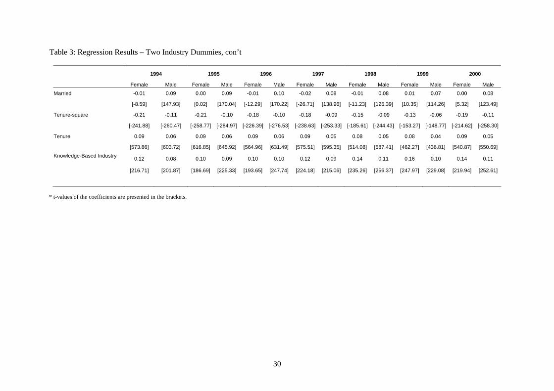
Table 3: Regression Results – Two Industry Dummies, con’t
1994 1995 1996 1997 1998 1999 2000 Female Male Female Male Female Male Female Male Female Male Female Male Female Male Married -0.01 0.09 0.00 0.09 -0.01 0.10 -0.02 0.08 -0.01 0.08 0.01 0.07 0.00 0.08
[-8.59] [147.93] [0.02] [170.04] [-12.29] [170.22] [-26.71] [138.96] [-11.23] [125.39] [10.35] [114.26] [5.32] [123.49]
Tenure-square -0.21 -0.11 -0.21 -0.10 -0.18 -0.10 -0.18 -0.09 -0.15 -0.09 -0.13 -0.06 -0.19 -0.11
[-241.88] [-260.47] [-258.77] [-284.97] [-226.39] [-276.53] [-238.63] [-253.33] [-185.61] [-244.43] [-153.27] [-148.77] [-214.62] [-258.30]
Tenure 0.09 0.06 0.09 0.06 0.09 0.06 0.09 0.05 0.08 0.05 0.08 0.04 0.09 0.05
[573.86] [603.72] [616.85] [645.92] [564.96] [631.49] [575.51] [595.35] [514.08] [587.41] [462.27] [436.81] [540.87] [550.69] Knowledge-Based Industry 0.12 0.08 0.10 0.09 0.10 0.10 0.12 0.09 0.14 0.11 0.16 0.10 0.14 0.11
[216.71] [201.87] [186.69] [225.33] [193.65] [247.74] [224.18] [215.06] [235.26] [256.37] [247.97] [229.08] [219.94] [252.61]
* t-values of the coefficients are presented in the brackets.

31
Table 4: Regression Results – Four Industry Dummies, Dependent Variable: Logarithm of hourly wage in Korean Won.* 1994 1995 1996 1997 1998 1999 2000 Female Male Female Male Female Male Female Male Female Male Female Male Female Male
(Constant) 7.18 6.98 7.39 7.04 7.44 7.15 7.55 7.27 7.56 7.20 7.57 6.83 7.68 6.92 [2359.04] [2472.80] [2428.99] [2592.81] [2366.75] [2558.74] [2363.52] [2597.50] [2151.97] [2369.76] [1985.76] [2103.02] [2068.51] [2160.12] Age 0.02 0.05 0.02 0.05 0.03 0.05 0.02 0.05 0.02 0.05 0.02 0.07 0.02 0.07 [130.75] [336.08] [110.38] [352.87] [144.59] [345.43] [129.82] [337.59] [115.09] [319.83] [85.32] [420.34] [92.70] [413.64] Age-squared -0.03 -0.06 -0.03 -0.06 -0.04 -0.06 -0.03 -0.05 -0.03 -0.05 -0.03 -0.08 -0.03 -0.07 [-147.29] [-324.80] [-130.76] [-336.52] [-167.90] [-331.95] [-153.95] [-321.26] [-143.48] [-302.21] [-99.80] [-411.73] [-112.51] [-392.97] High School 0.21 0.17 0.23 0.19 0.23 0.21 0.25 0.21 0.22 0.20 0.28 0.19 0.25 0.21 [286.39] [332.96] [303.14] [375.70] [288.32] [380.05] [294.25] [369.88] [230.90] [324.30] [271.33] [284.03] [256.16] [310.73] 2-year college 0.32 0.28 0.35 0.31 0.34 0.35 0.35 0.36 0.33 0.34 0.36 0.31 0.36 0.34 [275.43] [367.87] [312.48] [430.88] [302.13] [444.88] [315.22] [460.95] [271.85] [421.19] [276.77] [355.63] [287.07] [389.20] 4-year college + 0.60 0.52 0.60 0.54 0.63 0.58 0.63 0.58 0.60 0.56 0.62 0.56 0.62 0.58 [490.39] [881.14] [530.88] [960.91] [560.28] [938.41] [560.71] [931.09] [498.86] [838.14] [490.95] [767.28] [510.69] [804.39] 30-99 employees -0.01 -0.04 -0.03 -0.04 0.01 -0.04 0.01 -0.05 -0.02 -0.05 0.03 0.00 0.01 0.00 [-17.66] [-85.18] [-42.55] [-90.08] [7.38] [-79.98] [10.65] [-104.05] [-25.25] [-90.12] [35.53] [6.93] [14.15] [5.27] 100-299 employees 0.01 -0.06 0.02 -0.05 0.02 -0.06 0.03 -0.07 0.02 -0.04 0.06 0.05 0.06 0.05 [14.54] [-99.19] [22.37] [-91.52] [24.62] [-110.97] [45.26] [-119.94] [25.97] [-76.92] [62.77] [74.67] [69.58] [79.59] 300-499 employees 0.05 -0.03 0.07 0.02 0.07 0.02 0.08 0.00 0.08 0.04 0.08 0.09 0.13 0.16 [41.67] [-42.21] [69.48] [20.30] [59.94] [26.24] [68.65] [0.07] [63.33] [47.27] [53.82] [99.20] [98.10] [173.67] 500+ employees 0.11 0.06 0.11 0.08 0.16 0.10 0.18 0.12 0.16 0.16 0.19 0.22 0.16 0.17 [146.02] [107.57] [147.25] [148.92] [204.34] [167.07] [220.27] [209.81] [186.34] [266.18] [192.80] [332.29] [170.72] [266.82]

32
Table 4: Regression Results – Four Industry Dummies, con’t *
1994 1995 1996 1997 1998 1999 2000 Female Male Female Male Female Male Female Male Female Male Female Male Female Male Married 0.00 0.09 0.00 0.09 -0.01 0.10 -0.02 0.08 -0.01 0.08 0.02 0.07 0.01 0.07 [-3.97] [147.67] [-2.46] [169.13] [-8.01] [170.98] [-21.75] [139.94] [-14.23] [125.74] [16.60] [114.44] [10.10] [121.34] Tenure-square -0.20 -0.11 -0.21 -0.11 -0.18 -0.11 -0.18 -0.10 -0.15 -0.10 -0.13 -0.07 -0.19 -0.11 [-242.42] [-270.47] [-264.70] [-297.14] [-227.00] [-282.28] [-242.73] [-263.69] [-188.02] [-259.72] [-151.54] [-161.47] [-212.36] [-271.52] Tenure 0.09 0.06 0.09 0.06 0.08 0.06 0.08 0.05 0.08 0.05 0.07 0.05 0.09 0.06 [560.45] [611.48] [613.28] [655.48] [556.93] [634.35] [574.00] [603.66] [511.48] [600.96] [451.92] [452.57] [528.48] [568.12] Knowledge-based Manufacturing -0.05 0.00 -0.06 -0.01 -0.05 0.05 -0.04 0.01 0.00 0.00 -0.08 -0.01 -0.08 -0.05 [-51.60] [3.16] [-66.49] [-13.33] [-50.66] [70.60] [-37.89] [13.77] [-1.77] [-3.45] [-69.14] [-16.05] [-68.41] [-65.19] Knowledge-based Services 0.14 0.10 0.10 0.12 0.10 0.12 0.12 0.11 0.13 0.13 0.14 0.11 0.13 0.14 [179.05] [189.50] [130.31] [225.26] [135.48] [229.55] [155.10] [217.10] [168.98] [255.96] [165.78] [190.42] [156.28] [234.62] Other Manufacturing -0.07 -0.03 -0.09 -0.03 -0.08 -0.01 -0.09 -0.02 -0.07 -0.03 -0.14 -0.06 -0.12 -0.08 [-92.74] [-64.86] [-124.97] [-73.34] [-114.49] [-21.20] [-121.97] [-39.65] [-89.84] [-59.68] [-160.91] [-122.59] [-137.01] [-161.57]
* t-values of the coefficients are presented in the brackets.

33
Table 5: Non-Discriminatory Percentages
1994 1995 1996 1997 1998 1999 2000
Two Industry Dummies:
Knowledge-based Industries 0.938 0.939 0.945 0.974 0.973 1.000 0.984
(0.00081) (0.00079) (0.00079) (0.00079) (0.00080) (0.00000) (0.00084)
Non – Knowledge-based Industries 0.907 0.930 0.941 0.940 0.942 0.944 0.962
(0.00073) (0.00072) (0.00073) (0.00074) (0.00076) (0.00080) (0.00078)
Four Industry Dummies:
Knowledge-based Manufacturing 0.771 0.793 0.820 0.828 0.844 0.801 0.800
(0.00119) (0.00113) (0.00116) (0.00117) (0.00123) (0.00136) (0.00127)
Non-Knowledge-based Manufacturing 0.757 0.771 0.790 0.783 0.786 0.752 0.766
(0.00088) (0.00087) (0.00090) (0.00091) (0.00095) (0.00100) (0.00097)
Knowledge-based Services 0.933 0.928 0.952 0.964 0.966 1.000 0.982
(0.00098) (0.00095) (0.00096) (0.00096) (0.00096) (0.00000) (0.00102)
Non-Knowledge-based Services 0.811 0.842 0.860 0.859 0.847 0.869 0.863
(0.00100) (0.00097) (0.00098) (0.00098) (0.00101) (0.00104) (0.00105)
Values are }ˆexp{ tkγ− , where tkγ is based on equation (11). Values in parentheses are standard errors for tkγ , used to construct confidence intervals in Figures 3 – 5.