Embed Size (px)
Citation preview

USING A 3D FINITE ELEMENT FORWARD MODELING CODE TO ANALYZE
RESISTIVE STRUCTURES WITH CONTROLLED-SOURCE
ELECTROMAGNETICS IN A MARINE ENVIRONMENT
A Thesis
by
JOSHUA DAVID KING
Submitted to the Office of Graduate Studies of Texas A&M University in partial fulfillment of the requirements for the
degree of
MASTERS OF SCIENCE
December 2004
Major Subject: Geophysics
USING A 3D FINITE ELEMENT FORWARD MODELING CODE TO ANALYZE
RESISTIVE STRUCTURES WITH CONTROLLED-SOURCE
ELECTROMAGNETICS IN A MARINE ENVIRONMENT
A Thesis
by
JOSHUA DAVID KING
Submitted to Texas A&M University in partial fulfillment of the requirements for the
degree of
MASTER OF SCIENCE
Approved as to style and content by: Mark E. Everett William Bryant (Chair of Committee) (Member) David Sparks Roger Sassen (Member) (Member) Richard Carlson (Head of Department) December 2004 Major Subject: Geophysics

iii
ABSTRACT
Using a 3D Finite Element Forward Modeling Code to Analyze Resistive Structures with
Controlled-Source Electromagnetics in a Marine Environment. (December 2004)
Joshua D. King, B.S., Keene State College
Chair of Advisory Committee: Dr. Mark E. Everett
Controlled-Source Electromagnetics (CSEM) is a method that has been used since
the 1980’s in the marine environment for determining electrical properties of the
subsurface. The marine method involves towing a transmitter that is routed through
power circuits onboard a sea going vessel. Receivers on the seafloor collect total electric
and magnetic fields which are produced as a result of interaction of the transmitter
generated primary fields with the seawater and subsurface.
Badea et al. (2001) coded an existing algorithm for solving Maxwell’s equations.
This finite element (FE) 3D forward modeling algorithm is used to simulate CSEM
experiments. As CSEM surveys can be very expensive, forward modeling can be highly
valuable as a tool to learn about the effects of certain geological parameters on the
electric and magnetic fields.
The objective of the present study is to model the changes in electromagnetic
response for a resistive disk and a more geometrically complex structure, which are rough
approximations of hydrocarbon reservoirs. The parameters that are varied in studying
these subsurface structures are the disk radius, disk depth, the transmitter frequency, the
transmitter location, and the structure orientation. The goal of the study is to determine
how these parameters affected the total electric field collected by the receivers and if the

iv
shallowest portion of the complex structure could be located. Locating the shallowest
portion of the structure is important in that it tests the ability of the marine CSEM method
to determine the “sweet spot” which is the best drilling site.
The resistive disk responses are analyzed as changes are made in the disk radius,
disk depth, transmitter frequency, and transmitter location. The results showed that a
disk of finite radius behaves similar to an infinite disk at short range and grades into
double half-space behavior at longer ranges. The frequency of the transmitter must be
tuned to the disk depth as certain frequencies will penetrate too shallow or too deep to
probe the disk. For the purpose of this study only one frequency is used to avoid re-
meshing of the forward modeling code; this is the basic frequency of commercial marine
CSEM systems. The disk depth plays an important role in determining whether its
response can be separated from that of the double half-space. A disk that is too shallow
has negligible response due to the fields traveling preferentially through the sediments
under the disk. Similarly a disk that is too deep will not be viewed by the receiver
because the fields attenuate above that depth. Moving the transmitter away from the
receivers causes a decrease in signal strength, but exhibits a greater capacity to
distinguish between the double half-space and infinite disk scenarios.
Once these parameters had been modeled and their relation to the electric field
responses understood, the disk was replaced by a more complex structure. To determine
if the shallowest portion of the structure may be located a study was undertaken to probe
the structure from different perspectives using different transmitter locations and
azimuths. It is determined that the geometry changes of the structure could not be
observed until the structure’s thickness is sufficiently large. Small changes in structure
v
responses for the three different orientations exhibited CSEM’s ability to observe the 3D
nature of the structure.
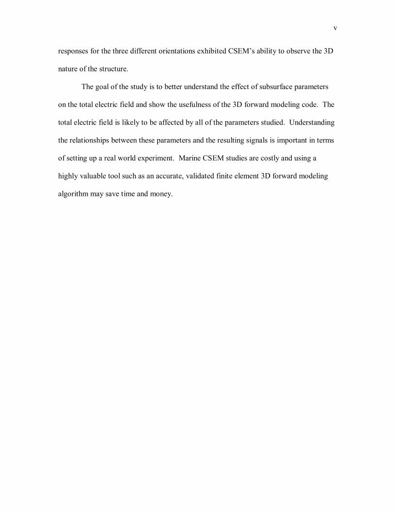
The goal of the study is to better understand the effect of subsurface parameters
on the total electric field and show the usefulness of the 3D forward modeling code. The
total electric field is likely to be affected by all of the parameters studied. Understanding
the relationships between these parameters and the resulting signals is important in terms
of setting up a real world experiment. Marine CSEM studies are costly and using a
highly valuable tool such as an accurate, validated finite element 3D forward modeling
algorithm may save time and money.

vi
ACKNOWLEDGEMENTS
I would like to thank Mark Everett for taking the time to answer all of my questions and for guidance on many subjects. I would like to thank Alfonso Benavides for helping me understand electromagnetics in all of its glory. I would like to thank Jamie Collins and Zach Long for help with this project. I would like to thank Katherine Kilday for being there through the whole process with support. I would like to thank my parents Beverly and David King for support given to me while working on this project.
vii
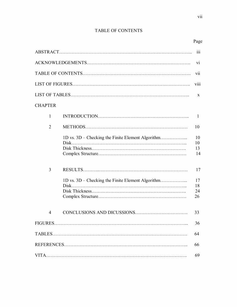
TABLE OF CONTENTS
Page
ABSTRACT………………………………………………………………………….. iii ACKNOWLEDGEMENTS…………………………………………………………. vi TABLE OF CONTENTS……………………………………………………………. vii LIST OF FIGURES…………………………………………………………………. viii LIST OF TABLES………………………………………………………………….. x CHAPTER 1 INTRODUCTION………………………………………………….. 1 2 METHODS………………………………………………………… 10 1D vs. 3D – Checking the Finite Element Algorithm……………... 10 Disk………………………………………………………………... 10 Disk Thickness……………………………………………………. 13 Complex Structure………………………………………………… 14 3 RESULTS………..………………………………………………… 17 1D vs. 3D – Checking the Finite Element Algorithm……………... 17 Disk………………………………………………………………... 18 Disk Thickness……………………………………………………. 24 Complex Structure………………………………………………… 26 4 CONCLUSIONS AND DICUSSIONS……………………………. 33 FIGURES…………………………………………………………………………... 36 TABLES…………………………………………………………………………… 64 REFERENCES…………………………………………………………………….. 66 VITA………………………………………………………………………………. 69
viii
LIST OF FIGURES
FIGURE Page
1 Cartoon view of Controlled-Source Electromagnetics…………………….. 36
2 Cartoon view of Double Half-Space w/Disk………………………………. 37
3 Cartoon view of Double Half-Space w/Complex Structure……………….. 38
4 1D vs. 3D at 1.0 Hz for short TX-RX offset...…………………………….. 39
5 1D vs. 3D at 1.0 Hz for long TX-RX offset...…………………………….. 40
6 1D vs. 3D at 0.1 Hz for short TX-RX offset...…………………………….. 41
7 1D vs. 3D at 0.1 Hz for long TX-RX offset...…………………………….. 42
8 Three lowest frequencies for the single-layered disk……………………... 43
9 Three middle frequencies for the single-layered disk……………………... 44
10 Three highest frequencies for the single-layered disk……………………... 45
11 0.1 Hz vs. 1.0 Hz for a single-layered disk………………………………… 46
12 0.1 Hz response for a single-layered disk…………………………………. 47
13 Disk burial depth plots for a single-layered disk…..……………………… 48
14 Transmitter locations for a single-layered disk……………………………. 49
15 Three lowest frequencies for the triple-layered disk……………………... 50
16 Three middle frequencies for the triple-layered disk……………………... 51
17 Three highest frequencies for the triple-layered disk……………………... 52
18 Single-layered disk vs. triple layered disk for 0.1 Hz…………………….. 53
19 Frequency range for complex structure at a 525 m burial depth…............. 54
20 Frequency range for complex structure at a 225 m burial depth…............. 55
ix
LIST OF FIGURES
FIGURE Page
21 Structure burial depth plots for a complex structure………….…………… 56
22 Transmitter locations for a complex structure at a 525 m burial depth…… 57
23 Transmitter locations for a complex structure at a 225 m burial depth…… 58
24 Transmitter locations for a ~336 m thick complex structure………………. 59
25 Transmitter locations for a ~675 m thick complex structure………………. 60
26 Transmitter locations for a ~675 m thick complex structure………………. 61
27 Complex structure orientated facing x-negative vs. facing x-positive...…... 62
28 Complex structure orientated facing x-negative vs. facing x-positive……... 63
x
LIST OF TABLES
TABLE Page
1 Local refinement parameters……………………………………………….. 64
2 Skin-depths for seawater and sediments………………………………….... 65
1
1. INTRODUCTION
1.1 - Previous Studies
The use of electromagnetics in the marine environment has been studied for about
two decades. The two methods used have been the passive magnetotellurics (MT)
method and the active controlled-source method. Studies have used MT to look at mid-
ocean ridge environments and as a tool for petroleum exploration. CSEM has also been
used for the study of ridge environments and more recently for petroleum exploration.
Marine electromagnetics has several advantages in areas where seismic has
difficulty in obtaining good quality data. In environments including salt bodies,
carbonates, or volcanics, seismic has been shown to produce poor results because of
scattering of the signal. Even the most advanced 3-D seismic methods may fail in these
settings (Hoversten et al, 1998). Such environments bode well for electromagnetics
because these bodies have resistivities which vary greatly from those of the surrounding
sediments. However electromagnetics is sensitive to bulk properties such as porosity and
not to sharp boundaries, which are more of a seismic target. Therefore, these two
methods (electromagnetic and seismic) should produce best results when used together
because they provide complementary information (Hoversten et al., 1998)
MT takes advantage of naturally occurring electromagnetic fields to estimate the
electrical properties of subsurface structure. In the marine environment, high frequency
signal components (roughly above 0.01 Hz) are attenuated as they propagate through the
seawater, leaving only the long frequency components with an appreciable amplitude.
This natural selection of frequencies allows for deep, albeit low-resolution studies. For
this reason, MT has been mostly used for deep crustal studies in the past. It was not until
2
Constable et al. (1998) designed a MT receiver (RX) which amplified the weak higher
frequencies, in the period range 3s to 1000s, that a new research area opened for the
method. MT may now be used for shallow crustal studies and as an additional tool for
petroleum studies.
The use of MT as a shallow marine investigative tool was emphasized by
Hoversten et al. (1998). Forward modeling results of a salt body were inverted to show
that the base of salt could be defined. This was done most successfully when pre-defined
boundaries from the seismic results were used in conjunction with the MT (Hoversten et
al., 1998). The next step was to field test the equipment.
A study was done by Hoversten et al. (2000) at the Gemini site in the Gulf of
Mexico. This site was chosen because the location of base of salt was considered to be
well-determined and an accurate comparison to previous seismic imaging was possible.
It was shown that MT may be used to accurately model the base of the salt body;
suggesting its usefulness to offshore petroleum exploration, because seismic had
difficulty imaging base of salt.
CSEM differs from MT in that the signal used is generated by a controlled
transmitter (TX) located on or near the seafloor. The proximity of the source to the
seafloor allows for the use of shorter frequencies which in MT would otherwise have
been attenuated by the depth of the water column. These introduced frequencies result in
higher resolution of the shallow geology (up to several kilometers in depth). This
method, like MT, is useful in mapping porosity. A system was developed and used
successfully to map near-surface porosity in coastal areas (Cheesman et al. 1990;
Cheesman et al. 1993). CSEM also has been used to study mid-ocean ridges and other

3
marine environments. Hydrothermal mounds have been studied with CSEM methods
(Nobes et al. 1992; Evans and Everett 1994; Cairns et al. 1996). Several surveys
gathered data from these environments and used inverse modeling to study the structure
of the ridge (Young and Cox 1981; Cox et al. 1986; Evans et al. 1991; Evans et al. 1994;
Constable and Cox 1996; MacGregor et al. 1998; Sinha et al. 1998; and MacGregor et al.
2001). Some of these studies, as well as others, used forward modeling to provide
understanding of the EM responses from typical geology (Evans et al. 1991; Evans and
Everett 1994; Flosadottir and Constable 1996, MacGregor et al. 2001; Unsworth 1994).
Flosadottir and Constable (1996) also used forward modeling for experiment design. The
problem of 2.5D forward modeling has been solved and used to aid in interpretation and
improve experimental design (Unsworth et al. 1993; Everett and Edwards 1992). The
2.5D forward modeling code models the use of a 3D source over a 2D structure. None of
these studies however, have employed a fully 3D forward modeling code which entails a
3D source used over a 3D structure.
Until now there have been no papers written on the subject of 3D controlled-
source electromagnetic forward modeling for its use in marine petroleum exploration.
The intent of this study is to analyze CSEM frequency domain responses of resistive
disks and a more complex structure which are rough representations of offshore
hydrocarbon reservoirs. This is done to simulate a marine CSEM experiment and also to
assess the utility of the 3D forward code.
4
1.2 - Controlled-Source Electromagnetics
The marine controlled-source electromagnetic method involves setting out
receivers on the seafloor which read signals from a transmitter towed behind and
powered from a ship (Figure 1). The power source onboard the ship generates an
alternating current which is sent down the cable to the transmitter. The current is
dropped down in voltage and runs through the transmitter, which in this case is a
horizontal dipole of ~ 100 m in length. A magnetic field is generated by the time-
dependent current. This magnetic field diffuses outwards through both the seawater and
seafloor. As the magnetic field passes through materials of various resistivities it will
generate secondary electric currents which in turn generate magnetic fields that are read
by the seafloor receivers previously placed on the seafloor. These data are analyzed to
interpret the resistive structure of the seafloor between the transmitter and the receivers.
The desired information is encoded in the fields propagating through the seafloor.
The seawater will also generate these secondary electric currents and magnetic fields but
these are typically used only to calibrate the apparatus since they encode known
information about seawater. The spatial decay of the fields can be characterized by the
skin depth equation:
500sd
fσ= ;
whereσ represents the conductivity of the medium in S/m, f is the transmitter frequency
in Hz, and sd is measured in m. Fortunately the seawater has a smaller skin depth than
the seafloor, so signals attenuate more rapidly in seawater and are read only by receivers
in close proximity to the transmitter. Further receivers read only the interesting seafloor
signals. The data from the received signals contains a vast and complicated amount of
5
resistivity information about the intervening material between transmitter and receiver,
thus making interpretation difficult at best. This is where forward modeling can enter the
picture, i.e. to help understand the experimental data. In forward modeling,
computational limitations dictate that only highly idealized models of actual geological
resistivity distributions can be evaluated. The idealizations should however contain
sufficient detail to model first-order response variations of actual structures.
1.3 - 3D Finite Element Code
1.3.1 - General Overview of the Code
The 3D forward modeling code used in this study is a finite element algorithm
developed by Mark Everett of Texas A&M University and Eugene Badea formerly of
Haliburton, Inc. The code has been used in the past for modeling electromagnetic well
logging in petroleum exploration (Badea et al, 2001). This code has been validated for
1D, 2D and 3D structures and solves the governing Maxwells equations as formulated in
terms of Coulomb gauged potentials. The forward problem is formulated in cylindrical
coordinates.
The finite element algorithm generates a cylindrical mesh formed from about
1000s of interconnected nodes. A wide range of geological structures may be modeled
since many mesh parameters (such as the node distribution) can be altered. A desired
structure or environment may be created by assigning elements various conductivities
based on the cylindrical coordinates of their constituent nodes. Once this is done, the
next step is usually to define the location of the transmitter with an external file which
6
controls parameters of the mesh. The code can then be run as a double half-space with a
uniform or a heterogeneous lower half-space representing the seafloor conductivity
(Figure 1). The code also permits the introduction of seafloor bathymetry, if required.
As the final result, after the finite element matrix system has been solved, each
node has its own value for the electric field and magnetic field. Every node can therefore
be visualized as a point receiver. The desired nodes must then be selected which would
represent experimental receiver locations. In this particular study some of the nodes on
the seafloor are representative of receivers. In localized areas where rapid changes occur
in the response, the mesh can be refined to better capture the true signature of the
response.
Local mesh refinement may be a very useful tool, especially for small TX-RX
offsets. The user refines a region by defining its boundaries, i.e. selecting the desired
radius, depth range, and azimuth desired. The tetrahedra in the refinement region are
subdivided dependent upon the level of refinement selected. New nodes are created,
which can be considered to be adding additional receivers to obtain a higher resolution.
A more complete description of the refinement process can be found in Badea et al.
(2001).
1.3.2 - General Description of the Math
Until recently finite difference (FD) methods were used to solve Maxwell’s
diffusion equations for heterogeneous media. A limiting factor of FD methods is that a
structured mesh is required. A second method, finite element (FE), allows for
unstructured mesh designs which are more flexible in terms of geometry and hence more
7
useful for modeling complicated geological variability. It is conventionally thought that
FE solvers demand overwhelming computational power; however a rapid increase in
computational technology has allowed for the desktop use of FE modeling. Badea et al.
(2001) used FE methods with Coulomb gauged electromagnetic (EM) potentials to solve
Maxwell’s diffusion equations.
Badea et al. (2001) formulated their FE solutions in terms of coupled vector-
scalar potentials (A, Ψ ) where A is the magnetic vector potential and Ψ is the electric
scalar potential. Accordingly the formulation has to satisfy two requirements: the normal
electric field is allowed to jump at interfaces while the tangential component must be
continuous and there must be no divergent or spurious modes in the EM fields. Badea et
al. (2001) used the vector/scalar approach because the vector magnetic potential, A, and
the electric scalar potential, Ψ , are continuous at the interfaces ensuring the first
requirement. The Coulomb gauge condition of A = 0∇ ⋅ ensures the second requirement,
that there are no divergent modes in the calculated EM fields.
The following is a simplified version of the mathematical development found in
Badea et al. (2001). Maxwell’s diffusion equations are valid only for the low frequencies
(such thatσ εω<< , where σ represents electrical conductivity, ε represents electric
permittivity, and ω represents angular frequency) used in CSEM. The basic equations
are
0 = iωµ∇× E H ; (1)
s = = σ∇ × +H J J E . (2)
The symbol 0µ is the magnetic permeability, sJ is the electric current density of the
source, and σ equals the electrical conductivity. Badea et al. (2001) apply the equation

8
0 = µB H to relate the magnetic induction and magnetic field vectors and the divergence
free conditions = 0∇ ⋅ J and = 0∇ ⋅ B to ensure there are no sources or sinks of current
and magnetic field, respectively, in the solution.
To increase ease of solving Badea et al. (2001) write E and H in terms of A and
Ψ , as follows:
≡ ∇ ×B A ; (3)
+ iω≡ ∇ΨE A . (4)
Equation (2) becomes:
0 0= ( + s iµ ωµ σ∇ × ∇ × + ∇Ψ)A J A . (5)
Badea et al. (2001) then use a method proposed by Biro and Preis (1989) incorporating
the term - ( )∇ ∇ ⋅ A to the left side of equation (5) to avoid asymmetric FE matrices.
These matrices could result in numerically unstable modes. The result is
0 0- ( ) - ( + = siωµ σ µ∇ × ∇ × ∇ ∇ ⋅ ∇Ψ) A A A J . (6)
The added term - ( )∇ ∇ ⋅ A disappears leaving the equation unchanged if
= 0∇ ⋅ A is satisfied. A vector identity 2- ( ) = -∇ × ∇ × ∇ ∇ ⋅ ∇A A A is applied by the
authors, showing that equation (6) is equivalent to a Helmholtz equation.
20 0 ( + = - siωµ σ µ∇ + ∇Ψ) A A J (7)
The authors then take the divergence of equation (5) to show that the divergence-free
condition = 0∇ ⋅ J is automatically enforced. Since equation (5) was altered (7) by itself
cannot be used to guarantee divergence free current density. To enforce = 0∇ ⋅ J , Badea
et al. (2001) augment (7) with the following equation
0[ ( + )] = 0iωµ σ∇ ⋅ ∇ΨA . (8)
9
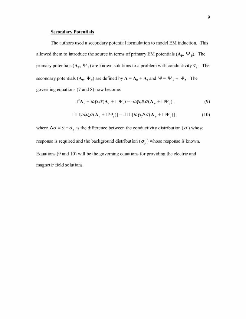
Secondary Potentials
The authors used a secondary potential formulation to model EM induction. This
allowed them to introduce the source in terms of primary EM potentials (Ap, Ψ p). The
primary potentials (Ap, Ψ p) are known solutions to a problem with conductivity pσ . The
secondary potentials (As, Ψ s) are defined by A = Ap + As and Ψ = Ψ p + Ψ s. The
governing equations (7 and 8) now become:
20 s 0 p + ( + ) = - ( + )s s pi iωµ σ ωµ σ∇ ∇Ψ ∆ ∇ΨA A A ; (9)
0 s 0 p [ ( + )] = - [ ( + )]s pi iωµ σ ωµ σ∇ ⋅ ∇Ψ ∇ ⋅ ∆ ∇ΨA A , (10)
where pσ σ σ∆ = − is the difference between the conductivity distribution (σ ) whose
response is required and the background distribution ( pσ ) whose response is known.
Equations (9 and 10) will be the governing equations for providing the electric and
magnetic field solutions.
10
2. Methods
This study consists of forward modeling the EM response from a marine
geological formation with embedded resistive structures. The transmitter location is
varied as well as the conductivities and geometries of the subsurface resistivity structure.
A primary goal is to understand how the signals received relate to the embedded
subsurface structures. Another goal is to produce simulated responses which can be used
to better understand experimental data and possibly to improve survey and equipment
design.
2.1 - 3D vs. 1D – Validating the 3D finite element algorithm
The first step is to validate the 3D finite element algorithm with an analytic code.
A double half-space model is used for the comparison. The 1D code solves for a
transmitter 100 m above the homogeneous seafloor. This is compared to the results of
the 3D finite element algorithm with a transmitter located 100 m above the seafloor
(z = 0) at the zero location (x = 0, y = 0). Both codes are run for short and long
transmitter-receiver offsets relative to the skin depth. The mesh boundary for the short
TX-RX offset is 1000 m and the mesh boundary for the long TX-RX offset is 10 km.
The top and bottom of the mesh are located at -1500 m and 1500 m respectively.
2.2 - Resistive Disk
The basic design of the mesh conforms to a double half-space with the upper
homogeneous half representing the seawater and the lower heterogeneous half-space
representing the sub-seafloor sediments. A finite water column thickness (e g air wave)

11
is neglected by assuming infinite water depth. The mesh top and bottom are still located
at -1500 m and 1500 m respectively, but the maximum radius is now 20 km. These
parameters will not be changed again. The first embedded seafloor structure to be
examined is a simple disk (Figure 2). The parameters that are varied include the
transmitter frequency, the disk radius, thickness, and burial depth in the subsurface
sediments. The structure (disk) is located in the lower half of a homogeneous double
half-space. The disk is intended to idealize the complicated geometry of a hydrocarbon
reservoir. The conductivities selected are chosen to represent those of actual seafloor
sediments containing hydrocarbons and were suggested by Steve Constable of Scripps
Institute of Oceanography. The conductivities of these bodies may be varied to represent
various sediment or rock types, as required.
An important fact to keep in mind throughout all modeling is that the same
receiver locations will be used. These are the nodes from 0 m to 20 km along the x-axis
(y = 0, z = 0). Each of the next sections will focus on one of the various parameters that
were studied.
2.2.1 - Disk Frequency and Radii
The first parameters studied are the disk radius and transmitter frequency. The
disk is placed at a burial depth of 525 m with its center at x = 0 and y = 0. The disk has
radial symmetry and is ~38 m in thickness. The transmitter location is on the x-axis at
-1000 m. This location is chosen because the seawater signals, which are undesired
noise, should have attenuated significantly by this distance. The transmitter is located at
100 m (z = -100 m) above the seafloor. The transmitter frequency range used is from

12
0.005 to 1.0 Hz. The models run consisted of a double half-space containing no disk
(double half-space); a 1250 m disk; 2500 m disk; 5000 m disk; and an essentially infinite
disk (20 km disk). The disk radii are chosen to represent the size of actual hydrocarbon
reservoirs of interest to marine CSEM explorationists.
The double half-space scenario and the infinite disk scenario represent the two
end-member responses while the finite-disk responses should fall in between. At short
TX-RX range the finite disks should behave like an infinite disk, but grade into double
half-space behavior at long range. Once the effects of this parameter on the total electric
field are satisfactorily understood the next step is to move the location of the transmitter.
2.2.2 - Transmitter Location
A series of transmitter locations are run from 0 m to -5000 m along the x-axis.
All of the other parameters listed in the previous section are used including the various
disk radii scenarios. The purpose of this experiment is to recreate, very roughly, the
towing of the transmitter along the seafloor. The idea is that each transmitter location is a
snapshot along the towline. This is done to see if the total electric field results will
behave in a predictable manner. The fields read by the receivers (which are always at 0
m to 20 km along the x-axis) should decrease in signal strength as the transmitter position
moves away. Insight into the separation of the response curves for the different modeled
disk radii in this way can be gained. Once these predictions are confirmed and the
separation of the disk curves understood, the disk depth is the next parameter altered.
13
2.2.3 - Disk Depth
Three disk depths: 225 m; 525 m; and 1012.5 m are selected which are
sufficiently separated from each other and conform to the pre-designed mesh boundaries.
The double half-space, finite disk, and infinite disk scenarios are used, a frequency of 0.1
Hz is also used, and a transmitter location of -1000 m on the x-axis is chosen. The main
objective of this set of numerical simulations is to determine how the TX-RX separation
affects the response for various disk depths. This parameter concludes the experiments
done on the disk; the next numerical experiments involve a change in the geometry of the
disk.
2.3 – Disk Thickness
Before the complex structure is introduced a three-layered disk is studied as a
intermediate case between the single-layered disk and the complex structure. The 3-
layered disk is three times the thickness of the single-layered disk, or ~ 112 m thick. The
top of the three-layered disk is located at the same 525 m burial depth as that of the
single-layered disk. The disk radii scenarios included the double half-space, 1250 m
disk, 2500 m disk, 5000 m disk, and an infinite three-layered disk. The parameter that is
altered in this model is the frequency. The main objective here is to analyze which
frequency is the most appropriate for detailed imaging of the three-layered disk. This is
decided by determining which frequency resulted in the greatest separation between the
double-half-space response curve and the infinite disk response curve. No further work is
done with this particular disk geometry and the complex geometric structure is studied
next.
14
2.4 - Structure
The next step is to introduce a more complex structure. The structure used is
suggested by Steve Constable of Scripps Institute of Oceanography and is based on
experience using marine EM for offshore exploration (Fig. 3). This structure is designed
to be a more geometrically accurate representation of a hydrocarbon reservoir than the
disk yet it still conforms to the underlying cylindrical geometry of the mesh. The
structure is three-tiered with the bottom layer being a full disk with the largest diameter
(3750 m), the second layer above is a 32πφ∆ = radian (¾ of a full 2π radians circle)
circle with a smaller radius, and finally an annulus segment, with an azimuthal radius of
2πφ∆ = radians (¼ of a full 2π radian circle), located on top (Figure 3). The parameters
varied are the transmitter location, transmitter frequency, the structure orientation, and
the thickness of the structure. The geometry of the structure is not varied as this is a
specific design.
The main objective of studying this structure is to understand the effect of
structure geometry on CSEM responses. A second objective is to examine the CSEM
responses to try to locate the thickest part of the structure where a well would be drilled.
Locating this “sweet spot” is done by using several transmitter locations around the
structure and comparing responses of receivers in a profile across the structure. Subtle
changes in the horizontal total electric field are related to the known location of the sweet
spot to determine whether and how these changes are indicative of this location
15
2.4.1 – Transmitter Frequency
The first objective is to determine which frequency is best to study the structure.
This is done by selecting the frequency which produces the greatest and most consistent
separation between the double half-space response curves and those of the structure. It is
of interest to determine whether a different frequency is more useful in imaging this
structure as compared to the best frequency for the single or triple-layered disk. The
structure is buried at 225 m and 525 m.
2.4.2 Structure Depth
The final experimental trial is to alter the depth of the structure. The same burial
depths of 225 m, 525 m, and 1012.5 m from the previous experiments are used. These
models are run to look for differences in the strength of the curves between those of the
structure and those of the single and triple layered disks.
2.4.3 – Structure Orientation
The geometry of this structure is not altered; however the transmitter is moved to
locations around the structure to view it from different perspectives. One problem with
this is that the 3D code was temporarily designed to use receivers in a line along the x-
axis. Instead of moving the TX, the structure is turned so that the open circle is facing
towards the negative x-axis and also the positive side of the x-axis. Although the code
could have been modified, an easier solution is to rotate the structure and leave the
transmitter in the same location of -1000 m on the x-axis. This simulates a perpendicular
tow across the broad-side of the structure. The last measure is to imitate the transmitter

16
on the y-axis by rotating the structure so that its open face is aligned with the y-axis.
This modeling experiment is done for burial depths of 225 m and 525 m. This
concludes transmitter location scenarios.
The objective of this section of experiments is to find if there is a difference in
response between the three different orientations that may indicate the location of the
shallow portion of the structure. In an actual experiment, for example, it is useful to
know how to best combine endfire and broadside TX tow responses in order to isolate the
sweet spot.
2.4.4 Structure Thickness
The final modeling is done to explore the changes in EM response caused by
thickening the structure. The structure has already been tested for a thickness of ~112 m
in all orientations (facing the negative x-axis, positive x-axis, and the positive y-axis).
The same models are run again at all transmitter positions and structure orientations for
structure thicknesses of ~ 336 m and 675 m. The model runs are done at a depth of 525
m, with a TX frequency of 0.1 Hz and a TX location of -1000 m on the x-axis. This
section concludes the methods.

17
3. Results:
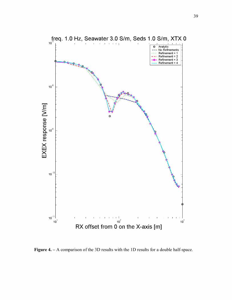
3.1 – 3D vs. 1D - Validating the 3D finite element algorithm The 3D finite element code is compared to the 1D analytic code. The first trials
for a frequency of 1.0 Hz, seawater conductivity 3.0 S/m and seafloor conductivity 1.0
S/m are run for short TX-RX offsets (from 0-1000 m). Four levels of refinement are
necessary to obtain an accurate match in the response (Table 1). The results show an
increasingly accurate match with the 1D analytic response as the mesh is refined (Fig. 4).
The figure indicates that local refinement is required to match the short offset receiver
analytic response. The next step is to model a much longer TX-RX offset (from 0-10
km).
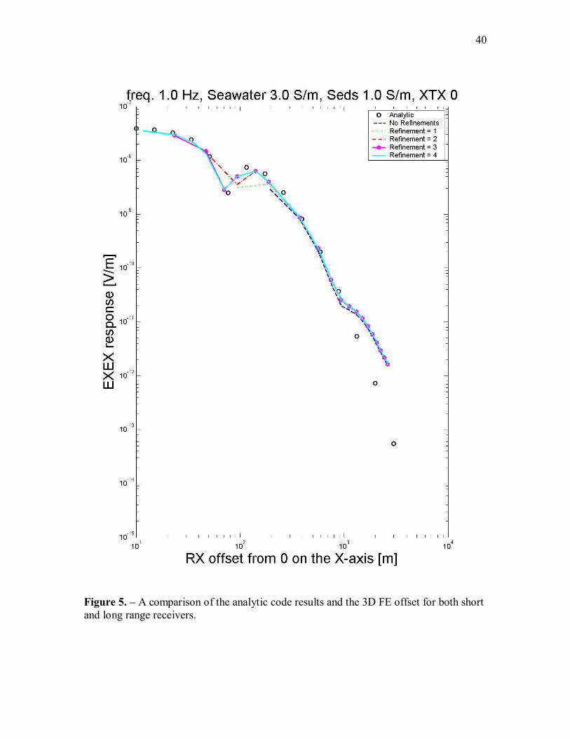
Long offsets are common in actual experiments where the ranges can be in excess
of 10 km. The long offset results proved to be less accurate even when including the four
local refinements (Fig. 5). Long offset total electric fields fell off more quickly with the
1D algorithm than with the 3D algorithm. As the analytic code has been well-tested to
provide accurate responses, changes had to be made to the 3D code. Through trial and
error it is found that the finite-element algorithm is very sensitive to the location of the
top and bottom of the mesh. However, a better match with the 1D algorithm is not
obtained for these models no matter how the geometry of the mesh was altered.
The original parameters used for the frequency and the conductivities are
changed. It is found again through running the code many times and comparing the
results to the 1D results that a product of the seafloor conductivity and frequency of order

18
one or greater ( S rad1 m s
σω > ) results in an inaccurate match. The decision is made to
keep the conductivities as close to the original value of σ =1.0 S/m while lowering the
frequency to obtain more accurate results. The reason for this is that real world
experiments would alter the frequency as the geologic conductivities cannot be altered.
Reasonable results are obtained for short TX-RX offset (Fig. 6) and long TX-RX
offset (Fig. 7) when the frequency was lowered to 0.1 Hz from 1.0 Hz while the mesh
size is shortened and widened. The ratio of height (z) to width (x and y) of the mesh is
about 1:3.3 respectively. The results for these runs of the 3D finite element results are
now reasonable; however they are still not as accurate as those of the short TX-RX offset.
Now that a mesh had been found that produced reasonable matches with the 1D analytic
algorithm for long TX-RX offsets the resistive disk can be introduced.
3.2 - Resistive Disk
3.2.1 - Transmitter Frequency and Radius
The resistive disk is inserted into the double half-space with the following
parameters; a range of frequencies (0.005 Hz to 1.0 Hz), seawater conductivity of 3.0
S/m, and a seafloor conductivity of 1.0 S/m. The newly introduced disk has a
conductivity of 0.01 S/m. The first results are for a transmitter location of z = -100 m,
and x = -1000 m with a variable radius of the disk (Fig. 8-11). This TX location is
chosen in order for the receivers (0-20 km) to be at least one seawater skin depth (912 m)
away from the transmitter when using the 0.1 Hz frequency. The seawater signals can be
19
considered noise in this case and are unwanted. This noise attenuates rapidly and a much
better subsurface signal to noise ratio is found at 1000 m from the transmitter location.
A study of the responses at varying transmitter frequencies is made to observe the
offset between the double half-space and the infinite disk curves, as well as the behavior
of the finite disks (1250 m, 2500 m, and 5000 m). When the disk is in the subsurface it is
buried at 525 m. A suite of frequencies is run from 0.005 Hz to 1.0 Hz including 0.01
Hz, 0.02 Hz, 0.05 Hz, 0.1 Hz, 0.2 Hz, 0.5 Hz, and 0.8 Hz. The skin depths of these
frequencies in both seawater and seafloor sediments can be found in Table 2.
The results show that for the group of lowest frequencies the curve separation is
not significantly decisive (Fig. 8). The lower frequencies show the greatest offset
between the double half-space curve and the infinite disk curve. However, the offset
occurs during the short range set of the receivers, from 625 m to about 4000 m. This
occurs for the three lowest frequencies: 0.005 Hz, 0.01 Hz, and 0.02 Hz. These low
frequencies show little to no curve separation at distances greater than 4000 m. This is
likely due to the receivers at these locations collecting signals from currents which have
preferentially been induced in the host medium beneath the disk. The next group of
frequencies better visualizes the disk.
The middle frequencies of 0.05 Hz, 0.1 Hz, and 0.2 Hz (Fig. 9) show a small
amount of curve separation at all receiver positions from 625 m to over 10 km. The
offset is mostly consistent along the x-axis receivers with little variation. These
frequencies appear to be probing the disk more consistently than the previous frequencies
because the curves of the double half-space results and the infinite disk results do not
overlap. A trend can also be noticed in the finite disks, where they grade from the
20
infinite disk behavior at short TX-RX offsets to double half-space behavior at long TX-
RX offset. As the frequency increases the gradation of the finite disks occurs at shorter
TX-RX offsets. This is seen by comparing long TX-RX offset finite curves for the
middle frequencies and high frequencies (Fig.11).
The highest frequencies include 0.5 Hz, 0.8 Hz, and 1.0 Hz (Fig. 10). The results
are similar to the previous group in that they show a consistent offset between the two
end-member curves along the receiver profile. Significant electromagnetic energy
appears to be propagating through the disk and not entirely under or above the disk. The
curve separation is slightly decreased from that of the previous group which may indicate
that not as much energy is getting through the disk. The pattern is tending towards an
overlap of the results of double half-space curve and the infinite disk curve. This may be
due to the decrease in depth of penetration as the higher frequencies are considered. The
finite disk response curves continue to show a decrease in the TX-RX offset at which the
curves follow the behavior of the double half-space. The depths to the disk are about one
skin depth (for these high frequencies) which means that less energy than in the case of
the middle frequencies propagates through the region of sediments containing the disk.
It is hypothesized that even higher frequencies would result in a complete overlap in the
double half-space scenario and the infinite disk scenario as the frequencies would not be
probing to the depth of the disk. However, at this time higher frequency scenarios cannot
be run as the finite element calculations become unstable. The ideal frequency for the
model we have been running is ~0.1 Hz (Fig. 12). This frequency provides the best
separation between the double half-space and infinite disk curves.
21
The finite disk responses are important in that they test the cylindrical 3D
capability of the FE algorithm. The responses show a gradation from infinite disk
behavior at short TX-RX offset and double half-space (no disk) behavior at long TX-RX
offsets. This gradation occurs at receivers which are located on the x-axis past the edge
of the buried disk. The lag occurs as the signals containing information about the edge of
the disk do not travel to the receivers directly above the disk, but to receivers further
down the x-axis. Therefore the edge of the finite disks can be roughly located with these
techniques.
The conclusions that can be made from this section are simple, yet very important
for experimental design. The frequency should be carefully chosen based on the depth of
the structure that is trying to be observed. A high frequency that yields an excessive
attenuation does not penetrate to the depth of the object. Low frequencies probe much
deeper and may only be observing the subsurface below the desired target. The other
important conclusion is that finite disks begin to behave similar to the double half-space
rather than the infinite disk at shorter TX-RX offsets as the frequency increases. This
model may be a useful in deciding which frequency to use in experiments.
3.2.2 - Disk Depth
The disk is buried at three different depths (Fig. 13). The original burial depth
used had been 525 m. The disk is raised to 225 m and lowered to 1012.5 m. These
depths are chosen somewhat arbitrarily mainly to observe the change in behavior of the
total electromagnetic fields. The two changes that are observed in Fig. 13 are the
22
strength of the total electric field and the separation between the different responses of
the different disk radii.
Each disk depth shows a significant difference in the behavior of its total electric
field response. The shallowest burial depth of 225 m below the seafloor shows little
separation between the double half-space scenario and the infinite disk scenario as signals
are probing mainly the sediments beneath the disk. The responses from the finite disks
grade from the infinite disk response to that of the double half-space response at large
TX-RX offset. The largest disk, 5000 m, as expected changes over at the greatest TX-RX
offset.
The next disk depth is the standard depth used in the other scenarios which is 525
m. The separation of the double half-space and infinite scenario curves has increased at
large offset, while decreasing slightly at short offset from the 225 m burial depth case.
The decrease could be due to the receivers sampling only shallow penetrating
electromagnetic fields which do not penetrate deep enough to sense the disk. The
opposite is true in the cases of large TX-RX offset as these receivers contain a significant
amount of data probing the depth ranges containing the disk. As in the case of the 225 m
burial, the finite disk responses grade from the infinite disk case to the double half-space
curve, but do so at slightly larger TX-RX offsets. This again is due to the fact that the
disk is buried deeper, so the seafloor signals from fields diffusing through the disk are not
read by the closer receivers. The slight lag between the location of the edge of the disk
and the location of receivers which apparently contain that information (in the form of the
beginning of the crossover from infinite-disk and no-disk) are seen once again.

23
The last depth chosen and the deepest is 1012.5 m. The offset in this case
between the double half-space and infinite disk scenarios is slightly increased from that
of the 525 m burial. Once again the short TX-RX offset data shows a decrease in
separation due to the deep burial of the disk. The finite disk curves behave in a
predictable manner in that they grade from the infinite disk curve to the double half-space
curve, but due so at receivers slightly further from zero than in the 525 m case. This is
also due to the increased depth of burial.
The depth of burial of the resistive body has a significant impact on the
differences between responses for models with various disk radii. The ability to
distinguish the curves increases significantly from a burial of 225 m to 525 m, but not
from 525 m to 1012.5 m. This is suggesting that another factor is controlling the curve
separation with depth. This factor may possible be related to the frequency of the
transmitter, since changing frequency effectively changes the depth of penetration.
3.2.3 - Transmitter Location
The transmitter is then moved away from zero along the x-axis in steps of 1000
m. The receiver results from offsets ranging from 0 to 20 km are predictable in that they
decrease in strength as the transmitter moves outward (Fig. 14). The TX location of XTX
= -1000 m is an exception in that it produces weaker responses than the next TX position
further away from zero (XTX = -2000 m). One reason for this may be that the receivers
close to the TX contain an increased amount of information from fields diffusing through
the seawater. The fields traveling through the seawater attenuate over shorter distances
and may be producing the weakened results at XTX = -1000 m.
24
The large TX-RX response of the infinite disk scenario for XTX = -1000 m
produces results varied from other TX locations. One explanation for the unusually
strong infinite disk response may be that the EM fields become trapped in the resistive
layer and diffuse along its length. This may be analogous to the wave guide phenomena
in seismic methods. The EM fields attenuate much less as they travel through the low
conductivity layer which results in anomalously strong responses at great distances.
The more distant transmitter locations exhibit weaker receiver signals, but provide
greater distinction between the various disk responses. At transmitter locations of -3000
m to -5000 m the curves for the double half-space and infinite disk scenarios are
separated at short TX-RX offset which was not the case for transmitter locations nearer to
zero. These scenarios show that information can be gained from certain locations which
more clearly display the subsurface geometry.
3.3 – Disk Thickness
Now that the one layered disk has been studied the next step is to increase the disk
thickness to observe the effects on the total electric fields. The top of this 3-layered disk
is again at 525 m depth beneath the seafloor. The models include the extremes of no-disk
and infinite-disk as well as the three finite disks (1250 m, 2500 m, and 5000 m). The
same range of transmitter frequencies, 0.005 Hz to 1.0 Hz is used. The transmitter is
located at -1000 m on the x-axis.
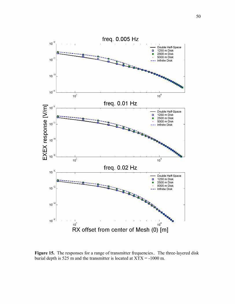
The results (Fig. 15-17) are very similar to those of a 1-layered disk. The lowest
three frequencies of 0.005 Hz, 0.01 Hz, and 0.02 Hz (Fig. 15) show a large separation

25
between the double half-space curve and the infinite disk curve at short offset. As in the
case of a one-layered disk, the long offset receivers show little separation in the readings
for the total electric fields. This is most likely due to the low frequency electromagnetic
fields preferentially propagating underneath the disk and probing the properties of the
sediments below. The main difference between these results and those of the 1-layered
disk is that the disk curves show a total electric field which is slightly stronger in the 3-
layered disk scenario. This is due to the thicker structure and results in a greater
separation from the double half-space scenario.
The 3-layered disk responses at the middle frequencies (Fig. 16) show very
similar properties to those of the 1-layered disk. They show constant curve separation
from receivers at 625 m to over 10 km. This again shows that the total fields contain
information about the disk at short and long TX-RX offset, unlike the low frequency
results. Once again the disk curves show slightly stronger total electric fields due to the
thickened disk, which results in a larger separation than in the 1-layer disk scenario. The
finite disks behave in a similar manner as the models with the single-layered disk.
However the crossover in behavior occurs at larger TX-RX offsets due to the increased
disk thicknesses.
The responses of the three highest frequencies (Fig. 17) are predictable. The
separation between the double half-space and infinite disk curves has decreased from that
of the lower frequencies due to a decrease in the depth of penetration so that induced
currents flow largely above the disk. The disk curves also show slightly increased
strengths in the total electric field from responses in the 1-layered disk scenario. Once

26
again the finite disks show crossover at greater TX-RX offsets than the single-layered
models (Fig. 18).
The thickened disk results reveal important information despite the slight
changes. An easily predictable result is that the strength of the total electric field
increases as the thickness of the structure increases. The finite disks crossover from the
response of an infinite disk to that of the double half-space at larger TX-RX offsets as the
thickness of the disk increases. The relative separation between the double half-space
and infinite disk curves remain about the same for each of the different transmitter
frequencies, as in the single-layered disk. Therefore the same frequency that is best for
the 1-layered disk is probably also best for the 3-layered disk. This may not be true for
drastically increased thicknesses which have not been examined here. Now that the
thickness parameter has been altered and its effects understood the geometrically
complex structure will be studied.
3.4 – Complex Structure
Evaluating the EM response of the structure which represents a rough design of a
hydrocarbon reservoir is the final step in this research. The description of the structure is
found in the experimental design section 2.4 and drawn in Fig. 3. The first objective is to
determine which frequency is best at locating this specific structure. The second and last
objective is to determine if locating the shallowest portion of the reservoir, and hence the
most productive part, is feasible.

27
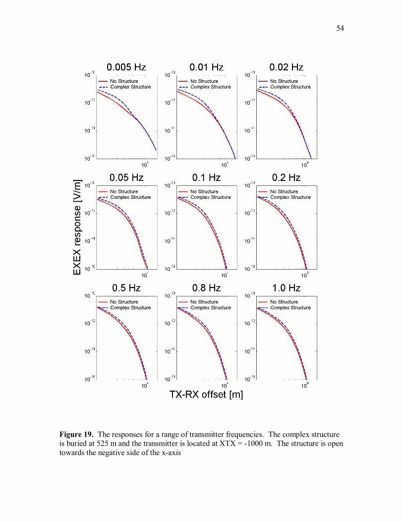
3.4.1 – Transmitter Frequencies
The range of frequencies is the same as used in the 3-layered disk. The first
results (Fig. 19) are for all 9 frequencies running from 0.005 to 1.0 Hz at a burial depth of
525 m and with the structure facing towards the negative side of the x-axis. The TX
location is at XTX = -1000 m and the structure is ~112 m thick. The results are very
similar to those of the 1-layered disk and the 3-layered disk. The lowest frequencies of
0.005 Hz, 0.01 Hz, and 0.02 Hz show a large difference between the double half-space
curve and the structure curve at short TX-RX offset. Once again this seems to indicate
that these frequencies, being the lowest, are propagating preferentially underneath the
structure which is buried at the same depth as the previous structures. This makes the
same sense as before and also suggests that the FE code generates consistent results.
The middle frequencies, consisting of 0.05 Hz, 0.1 Hz, and 0.2 Hz, show results
consistent with previous structures. The offset at small range has decreased from the
lowest frequencies, but the long range receivers are beginning to show a difference
between the double half-space response and that of the structure. An important note is
that the structure is finite yet is still being observed by the receivers over 10 km (several
skin depths) distant. The infinite curves of the single and three-layered disk show an
offset from the double half-space larger than that of the structure. This predictable fact
ensures that the FE code is working in accordance with expectations.
The three highest frequencies also begin to show a predictable decrease in offset
between the double half-space response and the structure response from that of the
middle three frequencies. The short range receivers show a separation between the two
curves which shows a slight decrease as the frequency increases. The long range

28
receivers show a convergence of the two curves indicating that the long range receivers
are not imaging the structure. This could be the result of the finite nature of the structure.
Looking back at the frequency range plots of the single and triple-layered disks it is seen
that even the highest frequencies still image their respective buried structures. This is
due to the fact that the disk plots include results of infinite radii. This seems to be
indicating further evidence that the solver is properly modeling the natural world as the
finite structure is producing weaker signals at long range than the infinite disks.
A parameter that is being tested simultaneously with the transmitter frequency is
the effect of the structures orientation. The code would be viewing the 3D nature of the
structure if the responses from the three different orientations facing the negative x-axis,
positive x-axis and positive y-axis displayed differences. The reason that the latter two
plots are not shown is because they exhibit the same responses as Figure 18 where the
structure is facing the negative side of the x-axis. The 3D nature of the structure is not
being imaged. The burial depth is then decreased to attempt to display differences in the
three orientations.
The next set of models in the frequency experiment included the same range of
frequencies and three orientations, but the burial depth is now 225 m. The responses
(Fig. 20) are very much the same in terms of the curve patterns. The one difference
which would be expected is that the 225 m burial produced stronger responses from the
structure model. This in turn caused a greater offset between the structure response
curves and the double half-space curves. The reason for the stronger structure responses
could be attributed to the structure being probed by higher powered signals as they have
traveled even less of a skin depth than those signals probing the deeper (525 m) structure.

29
The three different orientations once again produced the same exact responses for a burial
depth of 225 m; indicating that the 3D nature of the structure is not being imaged..
The main purpose of this frequency range experiment is to decide which
frequency was ideal for looking at this structure and to show the 3D nature of the
structure. The frequency that is chosen in this case was 0.1 Hz. This is the same
frequency that was chosen for the single and triple-layered disk. The reason that this
frequency is chosen is because it exhibited the most consistent offset over the range of
receivers from about 600 m to over 10 km. This frequency will now be used in the
second determination for locating the shallowest part of the structure. The 3D nature of
the structure is not displayed in the responses as all three orientations at both burial
depths of 225 m and 525 m produced the exact same curves.
3.4.2 – Structure Depth
The structure is buried at the same three depths as that of the single-layered disk
(225 m, 525 m, and 1012.5 m). The responses (Fig. 21) are similar to those of the single-
layered disk. At a burial depth of 225 m the structure is imaged well at short to middle
ranges, but at ranges approaching 5000 m the structure responses are weaker as the
receivers at these distances contain more information about the sediment below the
structure than the structure itself. The opposite is true for the second two burial depths.
A burial depth of 525 m produces the strongest offsets of double half-space responses and
structure responses past about 1000 m on the x-axis. The receivers located before 1000
m are reading signals more dominated by the sediments above the structure then the
receivers located after 1000 m. This pattern is exhibited even more so in the 1012.5 m

30
burial depth. The receivers located 2000 m from zero and beyond show the strongest
differences between the double half-space curves and the structure curves.
This information contained in Fig. 21 is important in much the same way as that
of the single-layered disk depth results (Fig. 13). The burial depth of the desired object is
an important piece of information to know when choosing the most appropriate
frequency.
3.4.3 - Structure Orientation
The second objective to locate the shallowest point of the structure is done by
looking at the structure from different perspectives and by using various transmitter
locations. The three different orientations are with the structure open face directed
towards the negative side of the x-axis, the positive side of the x-axis and the positive
side of the y-axis. The structure is observed from six transmitter locations moving away
from XTX = 0 m and from two burial depths (225 m and 525 m). The TX frequency
used is 0.1 Hz and the thickness of the structure is ~112 m. The strengths of the signals
decrease as the transmitter is moved away from the structure. The double half-space
curves and the structure curves show a separation which decreases as transmitter position
moves further from the center of the mesh. Now that the general characteristics of these
curves have been covered, the difference between the orientations will follow.
The three different orientations listed above are chosen to look at the structure
from different sides to look for slight variations which may indicate certain aspects of the
structure’s geometry. The responses for the three orientations are identical for the burial
depth of 525 m (Fig. 22). The same is true for the burial depth of 225 m (Fig. 23). This
indicates that the signal is not changing despite changes in the geometry of the

31
subsurface. This is not to say that any structure would not result in a signal change, only
perhaps structures of this scale. The fact that there is no difference in these six plots
seems to indicate that the small changes in the geometry of the structure cannot be seen
with this particular experimental design. This further indicates that locating the
shallowest portion of the structure where a well might be located cannot be found with
this design. The next and last parameter to alter in this study is the thickness of the
structure.
3.4.4 – Structure Thickness
The structure is thickened from its original (~112 m) to ~336 m and ~675 m. The
depth of burial remains at 525 m and the frequency stays at 0.1 Hz. The transmitter
locations move out from 0 m to -5000 m on the x-axis in steps of 1000 m.
The first increase in thickness from ~112 m to ~336 m shows no significant
difference in the responses (Fig. 24). The thickness increase does cause the total field
strength to increase as the amount of travel distance through the structure has increased
relative to the distance traveled through the sediments. Despite tripling the thickness the
three different orientations show no difference in their responses indicating that the
geometric changes in the structure are still not observed in the responses.
The last thickness increase is from ~336 m to ~ 675 m and exhibits responses
(Fig. 25, 26) which show that the structure is not radially symmetrical. The offset
between the structure curves and the double half-space curves again increased due to the
thickness of the structure increasing. An additional plot (Fig. 27) has been created to
better exhibit the differences between the two orientations. The plot compares the

32
response curves from the structure’s open side facing the negative side of the x-axis and
facing the positive side of the x-axis. The differences between the two orientations
responses can be seen in the receivers at short offset from the zero location at TX
locations of -3000 m, -4000 m, and -5000 m.
When the structure is facing the negative side of the x-axis it produces a stronger
response than when it is facing the positive side of the x-axis (Fig. 28). Since the
receivers are on the positive side of the x-axis this response is predictable as the signals
are traveling through a greater portion of the structure when it is facing open towards the
negative side of the x-axis. When the structure is open towards the positive side of the
axis more of the sediments are being probed, the main difference being the sediments in
the open segment of the structure. These responses do not seem to directly indicate
where the shallowest portion of the structure is located. However it has been shown that
the 3D nature of this structure can be seen in the response curves.
The conclusion of these trials is that the shallowest portion of the resistive body
cannot be imaged with these parameters, but the 3D nature of structures can be observed.
The 3D nature of the structure may not be well defined from these experiments, but they
have been observed. It may be that higher frequencies may better display the 3D
structure.
33
4. Conclusion and Discussion
The use of a finite-element 3D forward modeling algorithm can be useful to
obtain information that will increase understanding of controlled-source EM responses.
It was shown that various size finite disks will behave as an infinite disk at short range
while grading into the behavior of a homogeneous double half-space at larger TX-RX
receiver offset. The larger the radius of the disk means that crossover occurs further from
the transmitter. Changing the disk depth from 225 m to 525 m resulted in significant
changes in the responses indicating that disk depth played an important role. However
the lack of significant change from 525 m to 1012.5 m indicated that there was another
parameter with significant effect involving the transmitter.
The two parameters that were shown to have a significant impact on the total
electric field were the transmitter location and the transmitted frequency. When multiple
transmitter positions were modeled the results showed a decrease in signal strength as the
transmitter moved further away, but showed greater separation between the infinite disk
and double half-space curves. Thus multiple transmitter locations can provide different
useful information. The transmitted frequency is important in that it determines the depth
to which the field will penetrate. A frequency of 0.1 Hz was chosen for these
experiments because it showed a constant separation in the double half-space curves and
the infinite disk curves, as TX-RX offset was varied, indicating that this frequency
imaged the disk well in the models that were run. Changes in the design of the
subsurface feature played an important part of the understanding of CSEM methods as
well.

34
The results for the geometrically complex structure showed that changes on the
scale of 100s of m could be seen in this experimental design. The first step in tripling the
thickness of the disk gave important information in that it confirmed an increase in signal
strength due to an increase in structure size. Although the lack of change in the complex
structure results at thicknesses of ~112 m and ~375 m, valued information was gained.
Once the structure was thickened six times the original it was learned that the 3D
geometric changes in structure is better resolved with these designs. However the model
suggests that the differences were small. It is hypothesized that higher frequencies and
additional electrical information (Ey) may better image the structure. These experiments
have been shown to result in useful information for real world experimental design with
CSEM as well as show the usefulness of this finite element 3D forward-modeling
algorithm.
The results for the experiments run may be simple, but are intuitive in terms of
EM methods, and validate the accuracy and precision of this 3D forward modeling code.
The code has shown results which validate the ideas of how EM works in a marine
environment, but at the same time reveals the limits in terms of knowledge of CSEM
methods. The problem of understanding the responses of CSEM methods is complex, but
through the use of this code it has been shown that CSEM can be used to locate certain
structures in the marine environment which may prove useful to the petroleum industry.
The numerical algorithm is extremely complex at best, but flexible and useful. Future
studies may be done with this code to create more stable results by determining which
mesh designs fit with which conductivities and transmitter frequencies. This study is

35
barely tapping a huge reservoir of information that can be gained in the use of this 3D
forward modeling algorithm.

36
FIGURES
Figure 1 – A cartoon of an experimental setup over a double half-space.
~100 m in length - z
- x + x
+ z y-axis coming out of sheet
Sediments – 1.0 S/m
TX-RX range – 1-26 km
Seawater – 3.0 S/m
RX separation – 625 m

37
Figure 2 – A simplified drawing of the experimental setup over a disk.
1250 m -20 km in radius
y-axis coming out of sheet
- z
+ x - x
+ z
~38 m thick
Disk – 0.01 S/m Disk Depth – 525 m
Seawater –3.0 S/m
Sediments – 1.0 S/m

38
Figure 3 - A simplified drawing of the experimental setup over a disk.
Maximum radius of 3750 m
Complex Structure Depth - 525 m+ z
- z
+ x - x
y-axis coming out of sheet
~112 m thick
Seawater – 3.0 S/m
Structure – 0.01 S/m
“Sweet spot” Sediments – 1.0 S/m
39
Figure 4. – A comparison of the 3D results with the 1D results for a double half-space.
40
Figure 5. – A comparison of the analytic code results and the 3D FE offset for both short and long range receivers.

41
Figure 6. – A comparison of the 3D results with the 1D results for a double half-space.

42
Figure 7. – A comparison of the analytic code and the 3D FE results for both short and long range receivers.

43
Figure 8. The responses for the lowest transmitter frequencies. The transmitter is located at XTX = -1000 m and the single-layered disk is buried at a depth of 525 m.

44
Figure 9. The responses for the middle transmitter frequencies. The transmitter is located at XTX = -1000 m and the single-layered disk is buried at a depth of 525 m.

45
Figure 10. The responses for the highest transmitter frequencies. The transmitter is located at XTX = -1000 m and the single-layered disk is buried at a depth of 525 m.

46
Figure 11. Results from a model with a transmitter position of XTX = -1000 m, and a disk depth of 525 m.

Figure 12. Results from a model with a 0.1 Hz transmitter frequency, transmitter position of XTX = -1000 m, and a disk burial depth of 525 m.

48
Figure 13. Plots of responses for three disk burial depths. The transmitter frequency is 0.1 Hz and the transmitter location is at XTX = -1000.

49
Figure 14. Plots of various transmitter positions for a single-layered disk. The transmitter frequency is 0.1 Hz. The disk burial depth is 525 m.
50
Figure 15. The responses for a range of transmitter frequencies.. The three-layered disk burial depth is 525 m and the transmitter is located at XTX = -1000 m.

51
Figure 16. The responses for a range of transmitter frequencies.. The three-layered disk burial depth is 525 m and the transmitter is located at XTX = -1000 m.

52
Figure 17. The responses for a range of transmitter frequencies.. The three-layered disk burial depth is 525 m and the transmitter is located at XTX = -1000 m.

53
Figure 18. The responses for a transmitter frequency of 0.1 Hz. The disk burial depths are 525 m and the transmitter is located at XTX = -1000 m.
54
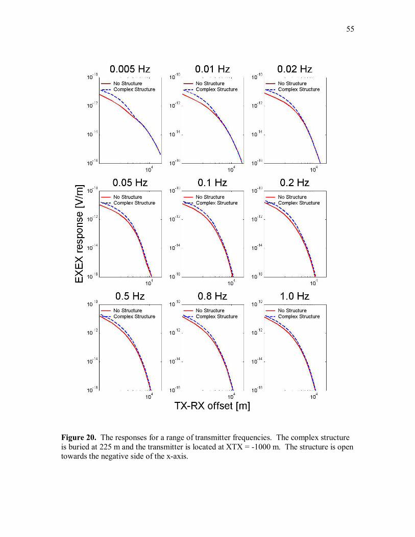
Figure 19. The responses for a range of transmitter frequencies. The complex structure is buried at 525 m and the transmitter is located at XTX = -1000 m. The structure is open towards the negative side of the x-axis
55
Figure 20. The responses for a range of transmitter frequencies. The complex structure is buried at 225 m and the transmitter is located at XTX = -1000 m. The structure is open towards the negative side of the x-axis.

56
Figure 21. A comparison of different burial depths for the complex geometric structure. The frequency is 0.1 Hz and the TX location is -1000 m.
57
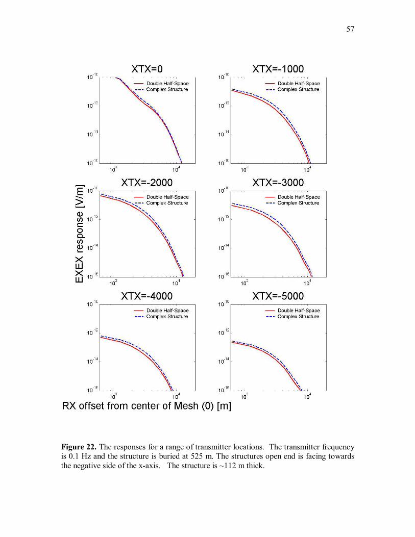
Figure 22. The responses for a range of transmitter locations. The transmitter frequency is 0.1 Hz and the structure is buried at 525 m. The structures open end is facing towards the negative side of the x-axis. The structure is ~112 m thick.
58
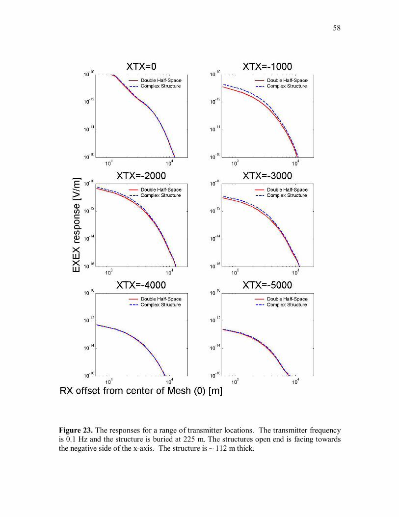
Figure 23. The responses for a range of transmitter locations. The transmitter frequency is 0.1 Hz and the structure is buried at 225 m. The structures open end is facing towards the negative side of the x-axis. The structure is ~ 112 m thick.

59
Figure 24. The responses for a range of transmitter locations. The transmitter frequency is 0.1 Hz and the structure is buried at 525 m. The structures open end is facing towards the negative side of the x-axis. The structure is ~ 336 m in thickness.
60
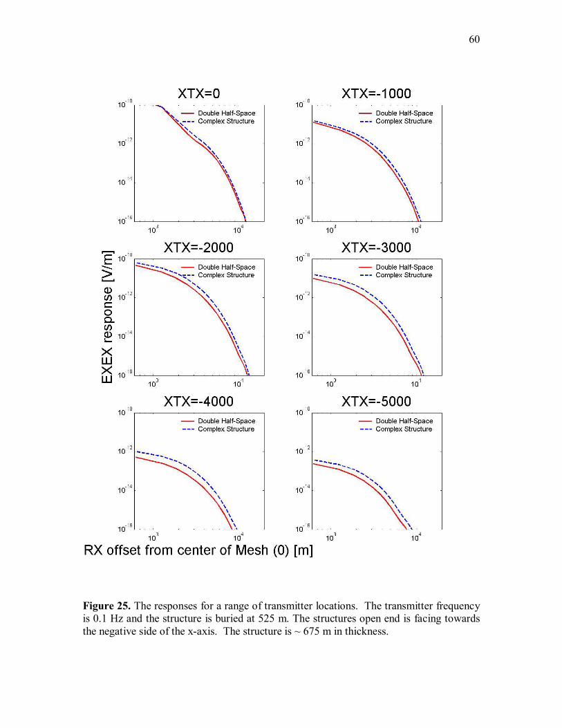
Figure 25. The responses for a range of transmitter locations. The transmitter frequency is 0.1 Hz and the structure is buried at 525 m. The structures open end is facing towards the negative side of the x-axis. The structure is ~ 675 m in thickness.
61
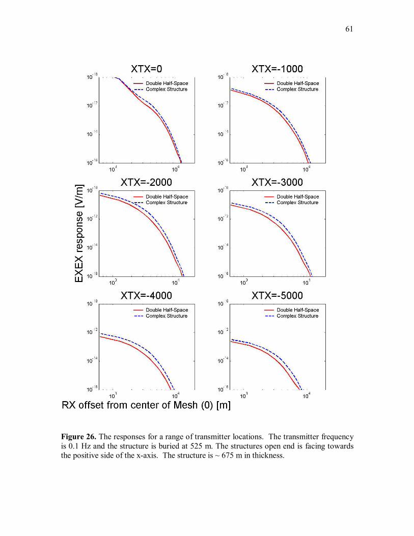
Figure 26. The responses for a range of transmitter locations. The transmitter frequency is 0.1 Hz and the structure is buried at 525 m. The structures open end is facing towards the positive side of the x-axis. The structure is ~ 675 m in thickness.

62
Figure 27. Structure responses for two of the three orientations. The frequency is 0.1 Hz, depth of burial 525 m, and the thickness of the structure is about 675 m.

63
Figure 28. Structure responses for two of the three orientations. The frequency is 0.1 Hz, depth of burial 525 m, and the thickness of the structure is about 675 m.
64
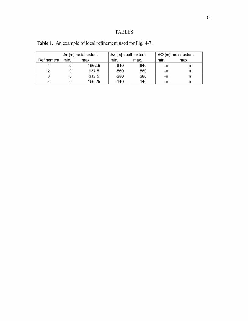
TABLES
Table 1. An example of local refinement used for Fig. 4-7. ∆r [m] radial extent ∆z [m] depth extent ∆Φ [m] radial extent Refinement min. max. min. max. min. max.
1 0 1562.5 -840 840 -π π 2 0 937.5 -560 560 -π π 3 0 312.5 -280 280 -π π 4 0 156.25 -140 140 -π π

65
Table 2. Shown are the skin depths for seawater and sediments Frequency
(Hz) Seawater (0.333 Ohm-m) skin depth
(m) Sediments (1.0 Ohm-m) skin depth (m)
1.0 289 500 0.8 323 559 0.5 408 707 0.2 645 1118 0.1 912 1581 0.05 1290 2236 0.02 2040 3536 0.01 2885 5000
0.005 4080 7071
.

66
REFERENCES
Badea, E.A., Everett, M.E., Newman, G.A., & Biro, O., 2001. Finite-element analysis
of controlled-source electromagnetic induction using Coulomb-gauged potentials, Geophysics, 66, 786-799.
Biro, O., & Preis, K., 1989. On the use of the magnetic vector potential in the finite element analysis of the three-dimensional eddy-currents, IEEE Trans. Magn., 25, 3145-3159. Cairns, G.W., Evans, R.L., & Edwards, R.N., 1996. A time domain electromagnetic
survey of the TAG hydrothermal mound, Geophysical Research Letters, 23, 3455-3458.
Cheesman, S.J., Edwards, R.N., & Law, L.K., 1990. A test of a short-baseline sea-floor transient electromagnetic system, Geophysics Journal International, 103, 431- 437. Cheesman, S.J., Law, L.K., & St. Louis, B., 1993. A porosity mapping survey in Hectate Strait using a seafloor electro-magnetic profiling system, Marine Geology, 110, 245-256. Constable, S., & Cox, C.S., 1996. Marine controlled-source electromagnetic sounding 2. The PEGASUS experiment, Journal of Geophysical Research, 101, 5519-5530. Constable, S.C., Orange, A.S., Hoversten, G.M., & Morrison, H.F, 1998. Marine Magnetotellurics for petroleum exploration Part I: A sea-floor equipment system, Geophysics, 63, 816-825. Cox, C.S., Constable, S.C., Chave, A.D., & Webb, S.C., 1986. Controlled-source electromagnetic sounding of the oceanic lithosphere, Nature, 320, 52-54. Evans, R.L., Constable, S.C., Sinha, M.C., Cox, C.S., & Unsworth, M.J., 1991. Upper crustal resistivity structure of the East Pacific Rise near 13° N, Geophysical Research Letters, 18, 1917-1920. Evans, R.L., & Everett, M.E., 1994. Discrimination of hydrothermal mound structures using transient electromagnetic methods, Geophysical Research Letters, 21, 501- 504. Evans, R.L., Sinha, M.C., Constable, S.C., & Unsworth, M.J, 1994. On the electrical nature of the axial melt zone at 13° N on the East Pacific Rise, Journal of Geophysical Research, 99, 577-588. Everett, M.E., & Edwards, R.N., 1992. Transient marine electromagnetics: the 2.5-D forward problem, Geophysical Journal International, 113, 545-561.
67
Flosadóttir, Á.H., & Constable, S., 1996. Marine controlled-source electromagnetic sounding 1. Modeling and experimental design, Journal of Geophysical Research, 101, 5507-5517. Hoversten, G.M., Morrison, H.F., & Constable, S.C., 1998. Marine Magnetotellurics for petroleum exploration, Part II: Numerical analysis of subsalt resolution, Geophysics, 63, 826-840. Hoversten, G.M., Constable, S.C., & Morrison, H.F., 2000. Marine Magnetotellurics for base of salt mapping: Gulf of Mexico field test at the Gemini structure, Geophysics, 65, 1476-1488. MacGregor, L.M., Constable, S., & Sinha, M.C., 1998. The RAMESSES experiment— III. Controlled-source electromagnetic sounding of the Reykjanes Ridge at 57° 45′ N., Geophysical Journal International, 135, 773-789. MacGregor, L.M., Sinha, M., & Constable, S., 2001. Electrical resistivity structure of the Valu Fa Ridge, Lau Basin, from marine controlled-source electromagnetic sounding, Geophysical Journal International, 146, 217-236. Nobes, D.C., Law, L.K., & Edwards, R.N., 1992. Results of a sea-floor electromagnetic
survey over a sedimented hydrothermal area on the Juan de Fuca Ridge, Geophysical Journal International, 110, 333-346.
Sinha, M.C., Constable, S.C., Peirce, C., White, A., Heinson, G., MacGregor, L.M., & Navin, D.A., 1998. Magmatic processes at slow spreading ridges: implications of the RAMESSES experiment at 57° 45′ N on the Mid-Atlantic Ridge, Geophysical Journal International, 135, 731-745. Unsworth, M.J., Travis, B.J., & Chave, A.D., 1993. Electromagnetic induction by a finite electric dipole source over a 2-D earth, Geophysics, 58, 198-214. Unsworth, M., 1994. Exploration of mid-ocean ridges with a frequency-domain
electromagnetic system, Geophysical Journal International, 116, 447-467. Young, P.D., & Cox, C.S., 1981. Electromagnetic active sounding near the East Pacific Rise, Geophysical Research Letter, 8, 1043-1046.
SUPPLEMENTAL SOURCES
Badea, E.A., Everett, M.E., Shen, L.C., & Weis, C.J., 2001. Effect of background fields on three-dimensional finite element analysis of induction logging, Radio Science, 36, 721-729.

68
Chave, A.D., & Cox, C.S., 1982. Controlled Electromagnetic Sources for Measuring Electrical Conductivity Beneath the Oceans, Journal of Geophysical Research, 87, 5327-5328.
Evans, R.L., Tarits, P., Chave, A.D., White, A., Heinson, G., Filloux, J.H., Toh, H.,
Seama, N., Utada, H., Booker, & J.R., Unsworth, M.J., 1999. Asymmetric Electrical Structure in the Mantle Beneath the East Pacific Rise at 17° S, Science, 286, 752-756.
Everett, M.E., & Constable, S., 1999. Electric dipole fields over anisotropic seafloor: Theory & application to the structure of 40 Ma Pacific Ocean lithosphere, Geophysical Journal International, 136, 41-56. MacGregor, L.M., & Sinha, M., 2000. Use of marine controlled-source electromagnetic sounding for sub-basalt exploration, Geophysical Prospecting, 48, 1091-1106. Sinha, M.C., Patel, P.D., Unsworth, M.J., Owen, T.R.E., & MacCormack, M.R.G., 1990.
An active source electromagnetic sounding system for marine use, Marine Geophysical Researches, 12, 59-68.
Warren, S., 2004. Sea Change: Exxon Mobil bets on new technology in the hunt for oil, Wall Street Journal, Vol. CCXLIV No. 33 (August 17, 2004), p. A1, A6. Webb, S.C., Constable, S.C., Cox, C.S., & Deaton, T.K, 1985. A Seafloor Electric Field
Instrument, Journal of Geomagnetism and Geoelectricity, 37, 1115-1129.
69
VITA
Joshua David King 459 Bakerville Road
Dartmouth, MA 02748
EDUCATION Texas A&M University, College Station, TX M.S. in Geophysics, December 2004 Thesis: Using a 3D finite element forward modeling code to analyze resistive structures with controlled-source electromagnetics in a marine environment Summer of Applied Geophysics Experience, Santa Fe, NM Geophysics Field Camp, July 2002 Indiana University, Cardwell, MT Geology Field Camp, July 2001 Keene State College, Keene, New Hampshire B.S. in Geology, May 2001 EXPERIENCE Summer 2003 GRADUATE RESEARCH ASSISTANT for Mark Everett at Texas A&M University, College Station, TX 09/02-05/04 GRADUATE TEACHING ASSISTANT for Dept. of Geology and Geophysics, Texas A&M University, College Station, TX 2000-2002 GEOLOGICAL TECHNICIAN for Steven Brackett of Brackett Geosciences, Keene, NH 2000 GEOLOGICAL TECHNICIAN for SVE Associates, Keene, NH 1997-2001 STUDENT WORKER/STUDENT SUPERVISOR for Mason Library, Keene State College, Keene, NH