Embed Size (px)
Citation preview

FINITE ELEMENT METHOD BASED
SIMULATIONS OF LOW FREQUENCY
MAGNETIC FIELD IN SEAWATER
A THESIS
SUBMITTED TO THE DEPARTMENT OF ELECTRICAL AND
ELECTRONICS ENGINEERING
AND THE GRADUATE SCHOOL OF ENGINEERING AND SCIENCE
OF BILKENT UNIVERSITY
IN PARTIAL FULFILLMENT OF THE REQUIREMENTS
FOR THE DEGREE OF
MASTER OF SCIENCE
By
Fatih Emre Şimşek
August, 2013

ii
I certify that I have read this thesis and that in my opinion it is fully adequate, in
scope and in quality, as a thesis for the degree of Master of Science.
_____________________________
Prof. Dr. Yusuf Ziya İder (Advisor)
I certify that I have read this thesis and that in my opinion it is fully adequate, in
scope and in quality, as a thesis for the degree of Master of Science.
____________________________
Prof. Dr. Hayrettin Köymen
I certify that I have read this thesis and that in my opinion it is fully adequate, in
scope and in quality, as a thesis for the degree of Master of Science.
____________________________
Assist. Prof. Dr. Satılmış Topçu
Approved for the Graduate School of Engineering and Science:
____________________________
Prof. Dr. Levent Onural
Director of the Graduate School
iii
ABSTRACT
FINITE ELEMENT METHOD BASED SIMULATIONS
OF LOW FREQUENCY MAGNETIC FIELD IN
SEAWATER
Fatih Emre Şimşek
M.S in Electrical and Electronics Engineering
Supervisor: Prof. Dr. Yusuf Ziya İder
August, 2013
Propagation properties of the electromagnetic waves in seawater are different
than in air (vacuum) due to electrical conductivity (σ) and high relative
permittivity (εr) of the seawater. Numerically it is hard to solve the
electromagnetic waves in seawater for the complex geometries. With the help of
the advances in the Finite Element Method (FEM) tools as well as the personal
computers, we have chance to analyze magnetic field of the complicated and
complex geometries of physical systems in seawater. In this thesis; an air-cored
multilayer transmitting coil is designed. Then the low frequency magnetic flux
density of this coil in different studies in seawater in COMSOL Multiphysics is
solved. In the first study; the magnetic flux density of the coil in air and in
seawater for different frequencies on different observation points is solved. In
the second study; the shielding effect of the material of the case of the coil as
well as the thickness of the case is analyzed. Specific materials as well as
thickness for the case are proposed. In the third study; the perturbation of the
magnetic flux density of the coil due to a metal plate is analyzed. The material
of the metal plate is taken iron and copper. Iron has high relative permeability (
r) and high electrical conductivity (σ). Copper has unity permeability ( 0) and
high electrical conductivity (σ). Effect of the high electrical conductivity on the
perturbation of the magnetic flux density on the observation point is analyzed.

iv
Effect of high relative permeability on the phase shift of the field on the
observation point is observed. A detection region for the plate and coil
geometries according to the attenuation of the secondary fields caused by the
eddy currents on the metal plate is proposed. In the last study; perturbation of
ambient Earth magnetic field due to a submarine is solved and how this
perturbation can be imitated by an underwater system, which tows a DC current
carrying wire is analyzed. These underwater systems are used to test detection
performance of magnetic anomaly detector (MAD) equipped aircrafts.
Keywords: Finite Element Method, COMSOL Multiphysics, Air-cored
multilayer coil, Metal detection in seawater, Magnetic anomaly detection.

v
ÖZET
DÜŞÜK FREKANSTA MANYETİK ALANIN DENİZ
SUYUNDA SONLU ELEMANLAR YÖNTEMİNE
DAYALI BENZETİMLERİ
Fatih Emre Şimşek
Elektrik ve Elektronik Mühendisliği, Yüksek Lisans
Tez Yöneticisi: Prof. Dr. Yusuf Ziya İder
Ağustos, 2013
Elektromanyetik dalgaların su içindeki yayılma özellikleri havadakinden
(vakum) suyun elektrik iletkenliği (σ) ve yüksek bağıl yalıtkanlık sabiti (εr)
yüzünden farklıdır. Karmaşık geometriler için elektromanyetik dalgaları deniz
suyu içinde nümerik olarak çözmek zordur. Sonlu Elemanlar Yöntemi (SEY)
araçlarındaki ve kişisel bilgiayarlardaki gelişmeler sayesinde deniz suyu içinde
karmaşık fiziksel sistemleri analiz etme şansımız vardır. Tezde; hava çekirdekli
çok katmanlı bir göndermeç sarımı tasarlanmıştır. Daha sonra bu sarımın
manyetik akı yoğunluğu deniz suyunda farklı durumlarda COMSOL
Çoklufizik'de incelenmiştir. İlk çalışmada; sarımın manyetik akı yoğunluğu
havada ve suda farklı frekanslarda ve farklı gözlem noktalarında çözülmüştür.
İkinci çalışmada; bobinin içinde bulunduğu gövdenin malzemesinin ve gövde
kalınlığının ekranlama analizi yapılmıştır. Gövde için belirli malzeme ve
kalınlık önerisinde bulunulmuştur. Üçüncü çalışmada; sarımın manyetik akı
yoğunluğunun metal bir plaka yüzünden bozulmasının analizi yapılmıştır. Metal
plakanın malzemesi demir ve bakır alınmıştır. Demir yüksek bir bağıl manyetik
geçirgenlik ( r) ve elektriksel iletkenliğe (σ) sahip olup; bakır ise birim
manyetik geçirgenlik ( 0) ve yüksek elektriksel iletkenliğe (σ) sahiptir. Yüksek
elektriksel iletkenliğin gözlem noktasındaki manyetik akı yoğunlunda yaptığı
etki analiz edilmiştir. Yüksek bağıl manyetik geçirgenliğin gözlem noktasındaki

vi
manyetik alanın fazındaki kaymaya etkisi analiz edilmiştir. Plaka ve sarım
geometleri için metal plaka üzerinde oluşan eddy akımlar tarafından yaratılmış
ikincil alanların sönümlenmesine göre bir saptama bölgesi önerilmiştir. Son
çalışmada ise; dünyanın manyetik alanının bir deniz altı tarafından bozulması
çözülmüş ve bu bozulma nasıl DC akım taşıyan bir teli çeken sualtı sistemi
tarafından taklit edilebilir analiz edilmiştir. Bu sualtı sistemleri manyetik
anomali detektörü (MAD) ile donatılmış hava taşıtlarının saptama
performanslarını test etmek için kullanılır.
Anahtar sözcükler: Sonlu Elemanlar Yöntemi, COMSOL Çoklufizik, Hava
çekirdekli çok katmanlı bobin, suda metal saptaması, Manyetik anomali
saptaması.

vii
To My Family

viii
Acknowledgements
I would like to express my gratitude to my supervisor Prof. Dr. Yusuf
Ziya İder for his instructive comments, invaluable guidance and continuing
support in the supervision of the thesis.
I would like to express my special thanks and gratitude to Prof. Dr.
Hayrettin Köymen and Dr. Satılmış Topçu for showing keen interest to the
subject matter and accepting to read and review the thesis.
My parents Cihan and Birgül Şimşek, and my brother Oğuz Şimşek
deserve special mention for their support and encouragement. I also would like
to thank my friends Taha Ufuk Taşcı, Ali Alp Akyol, Güneş Bayır, Durmuş Ali
Taşdemir, Fatih Süleyman Hafalır, Necip Gürler and especially Merve Nur
Çenesiz for their support and friendship.

ix
Contents
1 INTRODUCTION 1
1.1 Metal Detectors..............................................................................2
1.1.1 Metal Detector Technologies............................................4
1.1.2 Coil Orientations of Metal Detectors................................5
1.2 Fluxgate Magnetometer...................................................................7
1.3 DC Magnetic Anomaly Detector.....................................................8
1.4 Scope of the Thesis..........................................................................9
1.5 Outline of the Thesis......................................................................10
2 THEORY AND NUMERICAL METHODS FOR LOW
FREQUENCY MAGNETIC FIELD IN SEAWATER 12
2.1 Introduction..................................................................................12
2.2 Formulation..................................................................................12
3 DESIGN OF AN AIR-CORED MULTILAYER COIL 16
4 CASE STUDIES 19
4.1 Magnetic Field of a Coil..............................................................19
4.2 Magnetic Field of a Shielded Coil...............................................32
4.3 Perturbation of the Magnetic Field Due to a Metal Plate............43
4.3.1 Iron Plate..........................................................................55
4.3.2 Copper Plate.....................................................................62
4.4 Magnetic Field Due to Current in Straight Wire.........................73
5 DISCUSSION & CONCLUSION 88

x
List of Figures
Figure 1.1: Coil configuration no. 1. .................................................................... 6
Figure 1.2: Coil configuration no. 2. .................................................................... 6
Figure 1.3: Coil configuration no. 3. .................................................................... 7
Figure 1.4: Coil configuration no. 4. .................................................................... 7
Figure 3.1: Geometry of an air- cored multilayer coil. ...................................... 16
Figure 4.1: The coil in the solution medium. ..................................................... 20
Figure 4.2: Coil, case and the solution domain in 2D view. .............................. 21
Figure 4.3: Generated mesh of the coil, case and the medium. .......................... 22
Figure 4.4: Observation arch: one meter from the center of the coil from 00 to
900. ...................................................................................................................... 23
Figure 4.5: All three frequencies on the same plot (in air). ................................ 24
Figure 4.6: All three frequencies on the same plot (in seawater). ...................... 24
Figure 4.7: Frequency 500 Hz in air and seawater. ............................................ 25
Figure 4.8: Frequency 1 kHz in air and seawater. .............................................. 25
Figure 4.9: Frequency 10 kHz in air (green) and seawater (blue). ..................... 26
Figure 4.10: Observation line: Red line from the origin of the coil to 80m @ 00
(r=0, z=0 to r=0, z=80m). ................................................................................... 27
Figure 4.11: All three frequencies (500 Hz, 1 kHz and 10 kHz) in air and
seawater. ............................................................................................................. 28
Figure 4.12: Frequency 500 Hz in air (blue) and seawater (green). ................... 29
Figure 4.13: Frequency 1 kHz in air (blue) and seawater (green). ..................... 30
Figure 4.14: Frequency 10 kHz in air (blue) and seawater (green). ................... 31
Figure 4.15: Coil, case and the solution medium. .............................................. 33
Figure 4.16: Generated mesh of the coil, case and the solution medium. .......... 34
Figure 4.17: Observations points (r=0, z=1 and r=1, z=0). ................................ 35
Figure 4.18: Magnetic Flux Density norm (T) vs Conductivity(S/m), f = 500Hz.
............................................................................................................................ 37

xi
Figure 4.19 : Magnetic Flux Density norm (T) vs Conductivity(S/m), f =
10000Hz. ............................................................................................................ 38
Figure 4.20: Magnetic Flux Density Norm (T) vs Conductivity(S/m), f = 500Hz.
............................................................................................................................ 40
Figure 4.21: Magnetic Flux Density Norm (T) vs Conductivity(S/m), f =
10000Hz. ............................................................................................................ 41
Figure 4.22: Effect of thickness @ 00
(r=0, z=1)................................................ 41
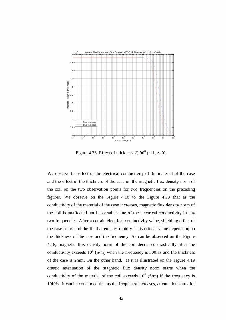
Figure 4.23: Effect of thickness @ 900 (r=1, z=0). ............................................ 42
Figure 4.24: Solution medium. ........................................................................... 44
Figure 4.25: Coil and the metal plate. ................................................................ 45
Figure 4.26: Generated mesh of the plate coil and the solution medium. .......... 46
Figure 4.27: Generated mesh of the plate. .......................................................... 47
Figure 4.28: Generated mesh of the coil. ........................................................... 47
Figure 4.29: Plate, coil and observation point. ................................................... 48
Figure 4.30: X component on the observation line (x=[4.95:5.05],y=0,z=0). ... 50
Figure 4.31: Y component on the observation line (x=[4.95:5.05],y=0,z=0). ... 50
Figure 4.32: Z component on the observation line (x=[4.95:5.05],y=0,z=0). .... 50
Figure 4.33: X component on the observation line (x=0,y=[-0.05:0.05],z=0). .. 51
Figure 4.34: Y component on the observation line (x=0,y=[-0.05:0.05],z=0). .. 51
Figure 4.35: Z component on the observation line (x=0,y=[-0.05:0.05],z=0). .. 51
Figure 4.36: X component on the observation line (x=0,y=0,z=[-0.05:0.05]). .. 52
Figure 4.37: Y component on the observation line (x=0,y=0,z=[-0.05:0.05]). .. 52
Figure 4.38: Z component on the observation line (x=0,y=0,z=[-0.05:0.05]). .. 52
Figure 4.39: Plate detection range. ..................................................................... 54
Figure 4.40: Element size 32cm (green) and 16cm (blue). ................................ 56
Figure 4.41: Eddy currents and surface current density on the bottom surface of
the iron plate when phase angle: 00. ................................................................... 58
Figure 4.42: Eddy currents and surface current density on the bottom surface of
the iron plate when phase angle: 750. ................................................................. 58
Figure 4.43: Perturbation of the field on the observation point due to iron plate
through the path (x, y=0, z=0). ........................................................................... 60

xii
Figure 4.44: Perturbation of the field on the observation point due to iron plate
through the path(x, y=0, z=-3.5). ........................................................................ 61
Figure 4.45: Element size 10cm (green) and 8cm (blue). .................................. 63
Figure 4.46: Generated mesh of the copper plate. .............................................. 63
Figure 4.47: Eddy currents and surface current density on the bottom surface of
the copper plate when phase angle of the current: 00. ........................................ 65
Figure 4.48: Eddy currents and surface current density on the bottom surface of
the copper plate when phase angle of the current: 750. ...................................... 65
Figure 4.49: Perturbation of the field on the observation point due to copper
plate, path(x, y=0, z=0). ..................................................................................... 67
Figure 4.50: Perturbation of the field on the observation point due to copper
plate, path(x, y=0, z=-3.5). ................................................................................. 68
Figure 4.51: Perturbation of the field on the observation point (x component),
iron vs. copper through the path(x, y=0, z=0). ................................................... 69
Figure 4.52: Perturbation of the field on the observation point (z component),
iron vs. copper through the path(x, y=0, z=0). ................................................... 70
Figure 4.53: Perturbation of the field on the observation point (x component),
iron vs. copper through the path(x, y=0, z=-3.5). ............................................... 71
Figure 4.54: Perturbation of the field on the observation point (z component),
iron vs. copper through the path(x, y=0, z=-3.5). ............................................... 71
Figure 4.55: Model of submarine. ...................................................................... 74
Figure 4.56: Submarine in the solution medium. ............................................... 74
Figure 4.57: Generated meshes of the submarine and the solution medium. ..... 76
Figure 4.58: Generated mesh of the submarine. ................................................. 76
Figure 4.59: Observation line (x=0, y=0, z=-40 to z=40). ................................. 78
Figure 4.60: Perturbation on the line of (x=0, y=0, z=-40 to z=40). .................. 78
Figure 4.61: Observation line (x=0, y=-25 to y=25, z=13). ............................... 79
Figure 4.62: Perturbation on the line of (x=0, y=-25 to y=25, z=13 ). 10m above
the submarine. .................................................................................................... 79
Figure 4.63: Perturbation on the line of (x=0, y=-25 to y=25, z=18 ). 15m above
the submarine. .................................................................................................... 80

xiii
Figure 4.64: Perturbation on the line of (x=0, y=-25 to y=25, z=28 ). 25m above
the submarine. .................................................................................................... 80
Figure 4.65: Current carrying wire system. ........................................................ 81
Figure 4.66: Wire and solution domain. ............................................................. 82
Figure 4.67: Generated meshes of the wire and the solution domain. ............... 83
Figure 4.68: Observation line (x=0, y=0, z=-40 to z=40). ................................. 84
Figure 4.69: Magnetic Flux Density norm on the line of (x=0, y=0, z=-40 to
z=40). .................................................................................................................. 84
Figure 4.70: Observation line (x=0, y=-25 to y=25, z=10). ............................... 85
Figure 4.71: Magnetic Flux Density norm on the line of (x=0, y=-25 to y=25,
z=10). .................................................................................................................. 85
Figure 4.72: Magnetic Flux Density norm on the line of (x=0, y=-25 to y=25,
z=15). .................................................................................................................. 86
Figure 4.73: Magnetic Flux Density norm on the line of (x=0, y=-25 to y=25,
z=25). .................................................................................................................. 86

xiv
List of Tables
Table 2.1: Electromagnetic properties of air and seawater for the frequency 1
kHz. .................................................................................................................... 15
Table 3.1: Dimensions of the coil. ..................................................................... 17
Table 3.2: New dimensions of the coil. .............................................................. 18
Table 3.3: Number of winding and impedance values of the coil. ..................... 18
Table 4.1: Properties of the computer used for the simulations. ........................ 19
Table 4.2: Magnetic Flux Density norm of the coil for 2mm thickness for
different materials. .............................................................................................. 35
Table 4.3: Magnetic Flux Density norm of the coil for 2mm thickness for
different conductivities of the material of the case. ........................................... 37
Table 4.4: Magnetic Flux Density norm for 1mm thickness for different
materials. ............................................................................................................ 38
Table 4.5: Magnetic Flux Density norm of the coil for 1mm thickness for
different conductivities of the material of the case. ........................................... 40
Table 4.6: Magnetic Flux Density of the coil on the observation point in
seawater. ............................................................................................................. 53
Table 4.7: Perturbation of the field on the observation point due to iron plate. . 60
Table 4.8: Perturbation of the field on the observation point due to copper plate.
............................................................................................................................ 67
Table 4.9: Effect of relative permeability and electrical conductivity on the
phase angle. ........................................................................................................ 72
Table 4.10: Perturbation of ambient Earth magnetic field due to submarine. .... 81
Table 4.11: Magnetic field of current carrying wire. ......................................... 87

1
Chapter 1
INTRODUCTION
Due to the recent developments in electronics as well as increase of the human
activity on the sea, underwater systems have become popular. With the ease of
new technological developments, many new applications have been designed;
old fashioned methods have been re-evaluated. Underwater telemetry and
control systems have been used for different applications. These applications are
related to communication, monitoring of wildlife, sensing, navigation, control
and monitoring of Autonomous Underwater Vehicles (AUV).
There are three different techniques that have been used in underwater
environment. These techniques are based upon acoustic [1,2,3,4,5], optic
[6,7,8,9] and electromagnetic [10,11,12] principles. As listed in [1], these
techniques have advantages and disadvantages compared to each other. Acoustic
based technology has these advantages; long range up to 20km, energy
efficient, precision navigation, low size and cost; in the meantime acoustic based
technology has these disadvantages; unable to transit water air boundary, poor
in shallow water, adversely affected by water aeration, ambient noise and
unpredictable propagation, latency, limited bandwidth detectable and impact on
marine life [1,2,3,4,5]. Optical based technology has advantages which are ultra-
high bandwidth and low cost; but also has disadvantages as well. These are
susceptible to turbidity and particles, marine fouling on lens faces, needs tight
alignment, very short range and difficult to cross water/air boundary [6,7,8,9].
Lastly; electromagnetic based technology has both advantages and
disadvantages; signal passes through ice, water/air and water/seabed boundary,
unaffected by water depth, unaffected by turbidity and bubbles, good non-line-
of-sight performance, immune to acoustic noise, immune to marine fouling, up

2
to 100 Mbps data rates, frequency agile capability, unaffected by multi-path, no
known effects on marine animals are the advantages, being sensitive to
electromagnetic interferences and limited range through water are the
disadvantages [10,11,12].
Electromagnetic based technology has many applications that exploit the
advantages of electromagnetic waves in seawater. The followings are some
applications of the electromagnetic based technology: real-time control of
Unmanned Underwater Vehicles (UUV) from shore, submarines and surface
vessels, wireless through-hull transfer of power and data, high-speed transfer of
data between UUVs and surface vessels, real-time transfer of sensor data from
UUVs when submerged, communications between UUVs and subsea sensors,
UUV distributed navigation systems for shallow harbors and ports, UUV
docking systems, subsea navigation beacons; asset location, asset protection,
subsea networks, data transmission from underwater sensors to surface or shore
without surface repeaters, harvest data from submerged sensors via Unmanned
Airborne Vehicles, communications; UUV to UUV, submarine to UUV, UUV
to Unmanned Surface Vehicle, UUV to Unmanned Airborne Vehicles, diver
communications (speech and texting), underwater navigation, underwater
sensing [13].
1.1 Metal Detectors
One of the most popular applications of electromagnetic based technology is
metal detectors in seawater [14,15,16,17,18]. One of the motivations of metal
detectors is to search treasures located deep below the oceans. Ships have been
transporting the riches of the world from port to port in their travels around the
world. Some ships ran into dangerous situations and sink with valuable items
under seawater during their journey. Trying to detect the location of such
shipwrecks is interest of some adventurers. They try to find caches of gold,
silver or anything else rumored to have been hidden somewhere in the

3
shipwreck [15]. When searching such shipwrecks, boat towed metal detectors or
magnetometers are used [16]. Metal detectors can be used to detect all types of
metals for reasonable depth [17]. Magnetometers can be used to locate iron and
steel at greater depth. If the adventurer can narrow the searching zone, a hand
held metal detector can be used. Hand held metal detectors feature either Pulse
or Broad Band Spectrum circuit to eliminate the effect of the minerals in the
seawater [18]. One another motivation of the metal detectors is to detect
underwater cables. Such cables are power and communication cables of
submarines. These cables which are installed in shallow waters have been buried
under the seabed. If these cables need to be repaired or relocated, they need to
be detected and tracked via metal detectors [19].
Magnetic field strength is measured via various different technologies. Each
technique has its own unique properties that make it more suitable for particular
applications. Devices which measure low fields (< 1 mT) are called
magnetometers and high fields (> 1 mT) are called gaussmeters [20].
Magnetometers are separated into vector component and scalar magnitude types.
Vector component type magnetometers are search coil, fluxgate, SQUID
(superconducting quantum interference device), magnetoresistive and fiber-
optic. Scalar type magnetometers are proton precession and optically pumped.
Sorts of gaussmeters are Hall Effect, magnetoresistive, magnetodiode and
magnetotransistor [21].
Metal detectors can be sorted according to the technology they use or according
to transmitting and receiving coil orientations. Each technology can have its
transmitting and receiving coil orientations and each orientation can have its
own technology [22,23]. Metal detectors use one of three technologies: very low
frequency (VLF), pulse induction (PI ) and beat-frequency oscillation (BFO).

4
1.1.1 Metal Detector Technologies
In very low frequency (VLF) technology there are two distinct coils. The outer
coil loop is the transmitter coil. It is a coil of wire. Electricity is sent along this
wire. The current moving through the transmitter coil creates an electromagnetic
field. The polarity of the magnetic field is perpendicular to the coil of wire. As
the current changes direction, the polarity of the magnetic field changes. If the
coil of wire is parallel to the ground, the magnetic field is constantly pushing
down into the ground and then pulling back out of it. As the magnetic field goes
back and forth into the ground, it interacts with any conductive objects it
encounters, causing them to generate weak magnetic fields of their own. The
polarity of the object’s magnetic field is directly opposite the transmitter coil’s
magnetic field. If the transmitter coil’s field is pulsing downward, the object’s
field is pulsing upward. The inner coil loop is the receiver coil which is another
coil of wire. It acts as an antenna to collect and amplify frequencies coming
from the target objects in the ground. When the receiver coil passes over an
object giving off a magnetic field, a small electric current goes through the coil.
This current oscillates at the same frequency as the object’s magnetic field. The
coil amplifies the signal and sends it to the control box of the metal detector
[24,25].
PI systems may use a single coil. This coil can be both transmitter and receiver.
The system also may have two or even three coils working together. This
technology sends powerful, short bursts (pulses) of current through a coil of
wire. Each pulse generates a brief magnetic field. When the pulse ends, the
magnetic field reverses polarity and collapses very suddenly, causing a very
sharp electrical spike. This spike lasts a few microseconds and results in another
current to run through the coil. This current is named the reflected pulse and is
extremely short, lasting only about 30 microseconds. Another pulse is then sent
and the process repeats. In a PI metal detector, the magnetic fields from target
objects add their “echo” to the reflected pulse, making it last a fraction longer

5
than it would without them. A sampling circuit in the metal detector is set to
monitor the length of the reflected pulse. By comparing it to the expected length,
the circuit can determine if another magnetic field has caused the reflected pulse
to take longer to decay. If the decay of the reflected pulse takes more than a few
microseconds longer than normal, there is probably a metal object interfering
with it [26,27].
In a beat-frequency oscillator (BFO) system there are two coils of wire. One
large coil is in the search head and a small coil is located inside the control box.
Each coil is connected to an oscillator that generates thousands of pulses of
current per second. The frequency of these pulses is slightly offset between the
two coils. When the pulses travel through each coil, the coil generates radio
waves. A small receiver within the control box collects the radio waves and
creates an audible series of tones (beats) based on the difference between the
frequencies. If the coil in the search head passes over a metal object, the
magnetic field caused by the current flowing through the coil creates a magnetic
field around an object. The object’s magnetic field interferes with the frequency
of the radio waves generated by the search-head coil. As the frequency deviates
from the frequency of the coil in the control box, the audible beats change in
duration and tone [22,28].
1.1.2 Coil Orientations of Metal Detectors
In the view of the orientation of the transmitting and receiving coil there are
different types of coil configurations in the metal detectors. Each of them has its
own advantages with respect to the techniques they are driven. The followings
are some common configurations of the transmitting and receiving coils.

6
Coil configuration no. 1 is called the GEM-3 configuration. There are three
concentric coils; two are transmitting and one is receiving (US Patent No.
5,557,206) in this configuration. Transmitter coil 1 is connected in an opposite
polarity to a small inner transmitter coil which creates a magnetic cavity at the
center where the receiver coil is placed. The two transmitting coils work
together to cancel (or buck) the source field at the receiver coil. This source
cancellation (or bucking) method provides a great increase in sensor dynamic
range and gives a resolution of parts-per-million level [29].
Coil configuration no. 2 is called GEM-5 configuration (US Patent No.
6,204,667). There are three concentric coils; one is transmitter at the center and
two are receiver on either side of and at equal distance from the transmitter. The
outputs from the two receiver coils are subtracted to cancel the primary signal
from the transmitter, providing a dynamic range and resolution similar to the
GEM-3 configuration [30].
Transmitter coil
1
Transmitter coil
2
Receiver coil
Figure 1.1: Coil configuration no. 1.
Receiver coil
2
Receiver coil
1
Transmitter
coil
Figure 1.2: Coil configuration no. 2.

7
There are two coils in the coil configuration no 3. One is the transmitter coil at
the origin (0, 0, 0). The other is the receiver coil perpendicular to the plane of
the transmitter coil. The receiver coil is at the point (0, y0, 0). Due to the
reciprocity, transmitter and receiver coils can be interchangeable, that is
transmitter coil can be receiver coil and receiver coil can be transmitter coil [19].
There are three coils in the configuration no. 4. One is the transmitter coil at the
origin and other two receiver coils are symmetrically away from the transmitter
coil. The plane of the transmitter coil is perpendicular to the receiving coils’.
The advantage of this configuration compared to the configuration 3 is that the
position of the detected material can be discriminated according to the detector
carrying device [31].
1.2 Fluxgate Magnetometer
The fluxgate magnetometer is a magnetic field sensor for vector magnetic field.
It can measure earth's field and resolve below one 10,000th
of that. It has been
used for navigation, compass work, metal detection and prospecting. It is easy to
z
X
y 0
y0
Figure 1.3: Coil configuration no. 3.
Figure 1.4: Coil configuration no. 4.
x
z
y 0
-y0 y0

8
construct. There are two style of design of it: designed with rod cores and
designed with ring cores. These cores are highly permeable cores which serve to
concentrate the magnetic field to be measured. The core is magnetically
saturated alternatively in opposing directions along any suitable axis, normally
by means of an excitation coil driven by a sine or cosine signal. Prior to
saturation the ambient field is guided through the core producing a high flux due
to its high permeability. When the core saturates, the core permeability falls
away to that of vacuum causing the flux to collapse. In the next half cycle of the
excitation waveform the core recovers from saturation and the flux because of
the ambient field is once again at a high level until the core saturates in the
reverse direction; the cycle then repeats. Although the magnetisation reversals
due to excitation, the flux from the ambient field operates in the same direction
throughout. A sense coil placed around the core will collect these flux changes,
the sign of the induced voltage indicating flux collapse or recovery [32].
1.3 DC Magnetic Anomaly Detector
Conventional detection of submarines has involved both acoustic and non-
acoustic techniques. Acoustic technique is the utilization of active and passive
hydrophones. These sound methods promise great range in the detection of the
submarines, [33]. Alternative techniques to detect submarines by hydrophones
were being studied in years 1917. One alternative was the use of magnetism.
Magnetic anomaly detection (MAD) is a passive method used to detect visually
obscured ferromagnetic objects by revealing the anomalies in the ambient Earth
magnetic field, [34]. The U.S experimentally tried a ship towed magnetic
detection device in 1918. This device had too limited a detection range and also
suffered from the presence of the magnetic signature of the towing ship. With
the outbreak of WW II, renewed interest occured in alternative detection
systems for anti-submarine warfare. There was a pressing need to devise a
means for them to be able to detect a submerged submarine for aircraft. One of

9
the devices that received renewed attention was the use of magnetic anomaly
detection. As early as 1941 magnetic detection devices (which measure changes
in the Earth's magnetic field) were developed in both Britain and the U.S. The
first use of these devices was in U.S K type blimps. This was followed by much
wider installation of MAD devices in ASW patrol aircraft. Most ASW aircraft
were equipped with MAD by 1943. Initially, the U.S. thought that MAD would
be a primary means of detecting submerged submarines. In use MAD was found
to be a system of limited usefulness. This was due to its very limited range and,
its inability to distinguish between sources of magnetic variance. Frequently,
wrecks or local magnetic disturbances were classified as submarines. This was
particulary true earlier in the war before experience with the system had
discovered its limitations. MAD in combination with sonobuoys proved more
useful by late war. In combination, MAD let an aircraft to localize a contact
made with sonobuoys and, the sonobuoys provided confirmation that the contact
was, indeed, a submarine. In this combination MAD became the secondary
system to the sonobuoy, the reverse of what was originally expected [35].
In order to test the detection performance of a magnetic anomaly detector
equipped aircraft, a submerged submarine is needed and practicaly it is hard to
have a submerged submarine any time it is necessary. Instead of having a
submerged submarine, a submerged system can be used to test the detection of a
magnetic anomaly detector equipped aircraft. In order to imitate the anomalies
on the ambient Earth magnetic field caused by the submarine, the submersed
system which tows DC current carrying wire can be utilized. Anomaly created
by this system can be tried to be detected by MAD equipped aircrafts.
Utilization of such systems cost less money and time than floating a submarine.
1.4 Scope of the Thesis
The Finite Element Method (FEM) has been developed and many commercial
FEM tools has been started to be utilized. One of the FEM tools is COMSOL

10
Multiphysics software. This is a general purpose-software platform, based on
advanced numerical methods, for modeling and simulating physics-based
problems [36]. In the thesis, we make use of this software. Not only FEM tools
have been developed but also physical memory and computation power of the
personal computers have been increased. With the help of the advances in the
FEM tools as well as the personal computers, we can analyze the complicated
and complex geometries of physical systems. In the thesis; we solve the low
frequency magnetic flux density of an air-cored multilayer coil in different cases
in seawater. In the first study the magnetic flux density of the coil in air and in
seawater for different frequencies on different observation points is solved. In
the second study; the shielding effect of the material of the case of the coil as
well as the thickness of the case is analyzed. Specific materials for the case as
well as thickness for the case are proposed. In the third study; the perturbation of
the magnetic flux density of the coil due to a metal plate which is firstly iron
then copper are analyzed. Iron has high relative permeability ( r) and high
electrical conductivity (σ). Copper has unity permeability ( 0) and high
electrical conductivity (σ). Effect of the high relative permeability and electrical
conductivity on the perturbation of the magnetic flux density of the coil is
observed. A detection region for the plate and coil geometries according to the
strength of the perturbation of the magnetic field is proposed. In the last study;
perturbation of ambient Earth magnetic field due to a submarine is solved and
how this perturbation can be imitated by a current carrying wire system so as to
test magnetic anomaly detector (MAD) equipped aircrafts is analyzed.
1.5 Outline of the Thesis
The outline of the thesis as follows. The second chapter discusses the theory and
numerical methods for low frequency magnetic field in seawater. In the third
chapter design of an air-cored multilayer coil is presented. Case studies of low
frequency magnetic field of the air-cored multilayer coil in seawater are

11
illustrated in the forth chapter. In addition, the perturbation of ambient Earth
magnetic field due to a submarine and how this perturbation can be imitated by
current carrying wire system is studied in the forth chapter. Finally, discussions
and conclusions are in the fifth chapter.
12
Chapter 2
Theory and Numerical Methods for
Low Frequency Magnetic Field in
Seawater
2.1 Introduction
Electromagnetic properties of seawater and air as well as governing equations of
propagation of electromagnetic waves in seawater are presented in this chapter.
Propagation properties of the electromagnetic waves in seawater are different
than in air (vacuum). The reason of this difference is that seawater has electrical
conductivity (σ) and high relative permittivity (εr). Electrical conductivity of
seawater varies from 1 to 8 (S/m). If the salinity of the sea is low the
conductivity is close to 1and if it is high, the conductivity is close to 8.
2.1 Formulation
In order to understand the behavior of the electromagnetic waves in seawater,
the governing equations must be known. Maxwell's equations predict the
propagation of electromagnetic (EM) waves travelling in seawater. To derive the
partial differential equation (PDE) system to be solved in the Magnetic Fields
interface under the branch of AC/DC for the physics section of the model in the
COMSOL Multiphysics, we start with Ampere's law:
e
D DH J E v B J
t t
. (2.1)

13
Now assume time-harmonic fields and use the definitions of the potentials:
B A , (2.2)
AE V
t
, (2.3)
Constitutive relationships between electrical and magnetic fields are the
followings:
0rB H , (2.4)
0rD E , (2.5)
where 0 0, are the permittivity and permeability of vacuum, with numerical
values:
7
0 4 10 (henry/m), (2.6)
12
0 8.854 10 (farad/m). (2.7)
In frequency domain, Ampere's law and electrical field are the followings:
eH E J j D , (2.8)
E j A . (2.9)
Electric displacement field (D) can be re-written according to the equations (2.5)
and (2.9) as following:
0rD j A . (2.10)
Magnetic field strength (H) can be re-written according to the equation (2.4) as
the following:
1 1
0rH B . (2.11)
14
Finally, when we put the equations (2.10) and (2.11) into the equation (2.8) and
re-arrange it, we find the PDA solved in COMSOL Multiphysics:
2 1 1
o r o rj A JeB . (2.12)
A linearly polarized plane EM wave propagating in the z direction can be
described in terms of the electric field strength Ex and magnetic field strength Hy
with [37],
0 exp( ),E E j t zx (2.13)
0H H exp( ).j t zy (2.14)
The propagation constant ( ) can be written in terms of permittivity ( ),
permeability ( ), and electrical conductivity ( ) by
j ,j j
(2.15)
where is the attenuation factor, is the phase factor, and 2 f is the
angular frequency. For a fixed frequency and conductivity, absorption
coefficient and wavelength in seawater can be written as the followings:
1/23 17.3 10 f dB / m , (2.16)
1/23 3.16 10 / f m . (2.17)
When α and λ are multiplied, how much electromagnetic energy in one
wavelength to be absorbed is found:

15
54.6(dB) (2.18)
The attenuation of 54.6 dB in one wavelength is a high value. This absorption
prevents the magnetic waves to penetrate long distances in seawater.
The speed of the electromagnetic wave in seawater is dependent upon the
frequency and electrical conductivity:
1/23c 3.12 x 10 f / (m/s). (2.19)
For example, the speed of the electromagnetic wave is 50x103 m/s and the
wavelength is 50m if the frequency is 1 kHz and the conductance of the
seawater is 4 (S/m). The speed of the electromagnetic wave in air is 3x10⁸ m/s
and the wavelength is 300x103 m if the frequency is 1 kHz. The following table
summarizes this example.
Medium Air (vacuum) Seawater
Speed of electromagnetic
wave (c) (m/s) 3x10
8 50x10
3
Wavelength (λ) (m) 300x103
50
Conductivity (σ) (S/m) 0 4 Permeability (µ) (H.m
-1) 1 1
Permittivity ( r) (F/m) 1 80
Table 2.1: Electromagnetic properties of air and seawater for the frequency 1
kHz.

16
Chapter 3
DESIGN OF AN AIR-CORED
MULTILAYER COIL
In this chapter; we design an air-cored multilayer coil in order to solve the
magnetic field of it in different case studies in seawater. We need the an air-
cored solenoid coil which is able to be steered with plausible current and power.
Since power consumption is an important criterion for an underwater system.
We steer the coil with 1 Ampere current through the studies. In order to be able
to steer the coil with 1 Ampere current, the coil has to have plausible impedance
value at low frequencies. We need to calculate the inductance of the coil so as to
calculate the impedance of it. The geometry and dimensions of an air-cored
multilayer coil is illustrated on the Figure 3.1.
Figure 3.1: Geometry of an air- cored multilayer coil.
O M I
C
B
W

17
We designate the coil with the dimensions on Table 3.1. We calculate the
inductance of an air-cored multilayer coil via Wheeler's formula, [38].
Dimensions Value (mm)
C (radial thickness) 125 mm
B(width or length) 100
W (diameter of the copper wire) To be determined
I (inner diameter) 250
M (mean diameter) 375
O (outer diameter) 500
Table 3.1: Dimensions of the coil.
According to Wheeler's formula, the design starts with the determination of the
inductance of the coil. Then the number of the windings is calculated and the
American Wire Gauge (AWG) number of the copper wire is decided. DC
resistance (R) of the wire is calculated either. P is linear packing density (the
wire diameter divided with the centre-to-centre wire spacing). P is taken as 0.8.
We decide 50 milliHenry for the inductance value of the coil. The necessary
design values are calculated by using the following equations:
2 27.87
3 9 10
N ML
M B C
(3.1)
2W
N B CP
(3.2)
214250
N MR
W
(3.3)
When we solve the equation (3.1) for N, we have 384 numbers of windings.
When we solve the equation (3.2) with this N for W, we have 4.56mm diameter
of the wire. We choose AWG 5 wire whose diameter is 4.621mm which is close
to the calculated one. We re-calculate C (radial thickness) with this new W via
the equation (3.2). We re-calculate the inductance of the coil with this new C
(radial thickness), and M (mean diameter) and we find 50.034 millihenry which
is closely 50 millihenry. We calculate the DC resistance (R) of the copper wire

18
via the equation (3.3) and find 0.47Ω. Then, we calculate the impedance of the
coil at 600 Hz as 2 2 600 0.05 188Z w L f L . The power
required to drive the coil is2 21 188 188P V I I R W . This power
consumption is plausible for an underwater system. In the thesis we make use of
this coil through the simulations.
Dimensions Value (mm)
C (radial thickness) 128
B (width or length) 100
W (diameter of the copper wire, AWG5) 4.621
I (inner diameter) 250
M (mean diameter) 378
O (outer diameter) 506
Table 3.2: New dimensions of the coil.
N (number of winding) 384 turns
L (inductance) 50 mH
Z (impedance @ 600Hz) 188 Ω
R (DC resistance ) 0.47Ω
Table 3.3: Number of winding and impedance values of the coil.

19
Chapter 4
CASE STUDIES
In this chapter, detailed analyses of magnetic field of the air cored multilayer
coil using 2D axial symmetric and 3D simulation of FEM models developed in
COMSOL Multiphysics are presented. In addition, analyses of perturbation of
ambient Earth magnetic field due to a submarine as well as analysis of magnetic
field of DC current carrying wire are presented. In each section these models are
described with respect to all aspects of FEM: geometry, physics, boundary
condition and mesh. The computer used for the FEM simulations needs to be
powerful in terms of central processing unit (CPU) and needs to have big
random access memory (RAM) to be able generate finer meshes and solve larger
matrices. The properties of the computer we used is illustrated on the Table 4.1.
Manufacturer: Hewlett-Packard Company
Model: HP Z800 Workstation
Processor:
Intel(R) Xeon(R) CPU X5675
@3.07GHZ 3.06GHZ (2 processors)
Installed memory (RAM): 64GB
System type: 64-bit Operating System
Table 4.1: Properties of the computer used for the simulations.
4.1 Magnetic Field of a Coil
In this section, low frequency magnetic field of the air-cored multilayer coil in
seawater and in air for three different frequencies of 500Hz, 1 kHz and 10 kHz
are studied in COMSOL Multiphysics. We observe the variations of the
magnetic flux density of the coil with respect to the three different frequencies

20
and seawater. The applied current to the coil is 1 Ampere. We take a cylinder as
a solution domain as illustrated on the Figure 4.1. The diameter and the height of
the cylinder is 50m. We put the coil in the solution domain as seen on the Figure
4.1 to have 2D axial symmetry. The coil is z-directed and at the origin of the
cylinder. The symmetry provides the problem to be solved with less physical
memory and processing power of the personal computer. This is an advantage
over 3D asymmetric geometries. In the model we put the coil into a case
(cylinder). This cylinder has 30cm radius and 15cm height and inside of it is air.
The case has no thickness. The coil, case and the medium can be seen in 2D
axial symmetry on the Figure 4.2.
Figure 4.1: The coil in the solution medium.
160m
160m x
y z

21
Figure 4.2: Coil, case and the solution domain in 2D view.
After modeling the geometry of the coil, Magnetic Fields interface is added
under the AC/DC branch for the physics selection of the model. This interface
solves the equation (2.12).
After adding physics for the model, we assign boundary conditions to the coil,
case and outer boundary of the solution domain enclosing the coil geometry.
Ampere’s Law is assigned to the coil and the case. In this condition, r is taken
1; σ is taken zero and εr is taken 1 since these domains are air. For the solution
domain enclosing the coil geometry we assign Ampere’s Law, too. If the
solution medium is air, r is taken 1; σ is taken zero and εr is taken 1. If the
solution medium is seawater, r is taken 1, σ is taken 4 (S/m) and εr is taken 80.
Boundary condition assigned to the edges of the solution medium is magnetic
insulation. The equation solved on this boundary is 0n A . We set the
tangential component of vector magnetic potential of these boundaries to zero.
In order to excite the coil, external current density is assigned to the coil domain.
The coil is excited in phi direction with respect to 2D axial symmetry.

22
After adding physics and boundary condition, we generate a mesh for the model
in order to discretize the complex geometry of the coil into triangular elements.
In order to get accurate results, in any wave problems, it is vital that wavelength
must be taken into account while generating meshes. According to [39],
maximum element size of the mesh elements must be at least one fifth of the
wavelength at the operating frequency. The meshing of coil, case and the
medium is on the Figure 4.3.
Figure 4.3: Generated mesh of the coil, case and the medium.
As the last step, we add frequency domain as study step and solver sequence for
the model so as to compute the solution.
We start post-processing of the magnetic flux density of the coil. Firstly we
observe the magnetic flux density of the coil on an arch. As can be seen on the
Figure 4.4, the observation arch is 1 meter away from the center of the coil from
00 to 90
0. The following plots show the change of the magnetic flux density
norm of the coil on the arc when the frequencies are 500 Hz, 1 kHz, 10 kHz and
the medium is air and seawater.

23
Figure 4.4: Observation arch: one meter from the center of the coil from 00 to
900.

24
Figure 4.5: All three frequencies on the same plot (in air).
Figure 4.6: All three frequencies on the same plot (in seawater).

25
Figure 4.7: Frequency 500 Hz in air and seawater.
Figure 4.8: Frequency 1 kHz in air and seawater.

26
Figure 4.9: Frequency 10 kHz in air (green) and seawater (blue).
Comparisons of the magnetic flux density of the coil for three frequencies in air
and in seawater are illustrated on the preceding plots. We observe on the plots
that the magnetic flux density norm is maximum at 00 (r =0, z= 1) and minimum
at 900 (r =1, z= 0) in one meter distance. Magnetic flux density norm at 0
0 (r =0,
z= 1) is almost two fold of magnetic flux density norm at 900 (r =1, z= 0). As
seen on the Figure 4.5, in air for three frequency (500 Hz, 1 kHz and 10 kHz)
curves coincide, on the other hand as seen on the Figure 4.6, in seawater 500 Hz
and 1 kHz are close to each other and 10 kHz differs from them. Blue curve is
500Hz, the frequency of green curve is 1 kHz and the frequency of red curve is
10 kHz. As the frequency increases, ratio of the magnetic flux density at 00 to
900 decreases. As seen on the Figure 4.7 and Figure 4.8, in air and seawater for
500 Hz and 1 kHz respectively, magnetic flux densities of the coil on the arc
coincide. As illustrated on the Figure 4.9, in air and seawater magnetic flux
density of the coil differ from each other.

27
Secondly; we observe the magnetic flux density of the coil on an observation
line which is from the center of the coil to 80m at 00 (r=0, z=0 to r=0, z=80m).
This observation line is illustrated on the Figure 4.10. Wavelength ( ) of
electromagnetic wave in seawater is 70m when the frequency is 500 Hz, 50m
when the frequency is 1 kHz and 16m when the frequency is 10 kHz. In the
following plots, we observe the attenuation of magnetic flux density of the coil
in air and seawater for each frequency.
Figure 4.10: Observation line: Red line from the origin of the coil to 80m @ 00
(r=0, z=0 to r=0, z=80m).

28
When we plot the magnetic flux density of the coil through this observation line
for three frequencies (500 Hz, 1 kHz and 10 kHz) in air and seawater, we see
that all of the plots coincide; it is not possible to discriminate them from each
other. This plot is illustrated on the Figure 4.11. In order to be able to
discriminate the plots, we plot them for three different frequencies and two
mediums in the following figures.
Figure 4.11: All three frequencies (500 Hz, 1 kHz and 10 kHz) in air and
seawater.

29
When the frequency is 500 Hz, wavelength ( ) of electromagnetic wave in
seawater is 70m. Comparison of the magnetic flux density of the coil in air and
seawater through the line (r=0, z=[69:71]) is illustrated on the Figure 4.12.
Magnetic flux density in seawater is 135.0639 10 (T) and in air is
111.1729 10 (T) at the point (r=0, z=70m). In one wavelength, the magnetic
flux density of the coil attenuates 62.8dB in seawater with respect to in air.
Figure 4.12: Frequency 500 Hz in air (blue) and seawater (green).

30
When the frequency is 1 kHz, wavelength ( ) of electromagnetic wave in
seawater is 50m. Comparison of the magnetic flux density of the coil in air and
seawater through the line (r=0, z=[49:51]) is illustrated on the Figure 4.13.
Magnetic flux density in seawater is 121.2856 10 (T) and in air is
115.8812 10 (T) at the point (r=0, z=50m). In one wavelength, the magnetic
flux density of the coil attenuates 76.4dB in seawater with respect to in air.
Figure 4.13: Frequency 1 kHz in air (blue) and seawater (green).

31
When the frequency is 10 kHz, wavelength ( ) of electromagnetic wave in
seawater is 16m. Comparison of the magnetic flux density of the coil in air and
seawater through the line (r=0, z=[15:17]) is illustrated on the Figure 4.14.
Magnetic flux density in seawater is 113.6698 10 (T) and in air is
92.1699 10 (T) at the point (r=0, z=16m). In one wavelength, the magnetic
flux density of the coil attenuates 81.5dB in seawater with respect to in air.
Figure 4.14: Frequency 10 kHz in air (blue) and seawater (green).

32
4.2 Magnetic Field of a Shielded Coil
Detectors, sensors and electronic circuitries of underwater systems are isolated
from seawater via water proof cases due to the fact that submerging the system
into seawater without isolating it from seawater damages the components of the
electronic systems. There are different decision criterions in the selection of the
material of the case of the underwater systems. The material of case has to be
water proof, hard, durable and rustproof. Selection of the material of the case is
also a vital decision step when the concerns of electromagnetic interference are
taken into account. The material of the case can affect the magnetic field of the
coil according to its electrical properties. Due to the electrical properties of the
case that are electrical conductivity ( ) and relative permeability ( r ), the
strength of the magnetic field can be attenuated. The attenuation of the magnetic
field of the coil is not only due to the permeability of the material of the case but
also eddy currents that are created on the surface of case. This effect is called the
shielding effect of the case on the magnetic field strength of the coil. In this
section, the effect of the electrical conductivity of the material of the case and
different thicknesses of the case on the magnetic flux density of the coil is
studied. We disregard permeability of the material of the case and other
electromagnetic interference sources. The studied materials are copper (Cu),
aluminum (Al), stainless steel and carbon mixed composite. These materials
have relative permeability ( r ) 1 and relative permittivity ( r ) 1 but they have
different electrical conductivity values.
We begin the analysis with the designation of the geometry of the models in
COMSOL Multiphysics. We take a solution domain as a cylinder whose height
is 50m, radius is 25m. We take the case whose inner length is 50cm and inner
radius is 25.5cm. We take a gap distance of 2mm between the outer radius of the
coil and the inner radius of the case. Two dimensional axial symmetric views of
the case, coil and the solution medium are on the Figure 4.15.

33
Figure 4.15: Coil, case and the solution medium.
After modeling the geometry of the coil and the case, Magnetic Fields interface
is added under the AC/DC branch for the physics selection of the model. The
equation solved in this interface is the equation (2.12).
After adding physics for the model, we have to assign boundary conditions to
the coil, the case and the solution domain enclosing the coil and the case
geometries. For the solution domain enclosing the coil and the case geometries
we assign Ampere’s Law. The solution medium is seawater, r is taken 1, σ is
taken 4 (S/m) and εr is taken 80 in this domain. The coil domain and inner of the
case domain are taken air, r is taken 1, σ is taken zero and εr is taken 1 in these
domains. Thickness domain of the case is the interested material. We assign
Ampere’s Law in this domain too. In this domain, r is taken 1, and εr is taken
1. Electrical conductance (σ) varies according to the material chosen. Boundary
condition of the edges of the solution medium is magnetic insulation. The
equation solved on these edges is 0n A . We set the tangential component of
vector magnetic potential of these boundaries to zero. In order to excite the coil,

34
external current density is assigned to the coil domain. The coil is excited in phi
direction with respect to 2D axial symmetry.
After adding physics and boundary condition, we generate a mesh for the model
in order to discretize the complex geometry of the coil into triangular elements.
Figure 4.16: Generated mesh of the coil, case and the solution medium.
As the last step, we add frequency domain as study step and solver sequence for
the model so as to compute the solution.
We study the shielding effect of thicknesses for 2mm and 1mm of the case for
three frequencies of 500Hz, 1 kHz and 10 kHz. Observation points of shielding
effect are on the Figure 4.17. Firstly, we observe the effect of the 2mm thickness
of the case for different materials, different electrical conductance values and
frequencies on the magnetic flux density norm at two points: (r=0, z=1) and
(r=1, z=0). Secondly, we observe the magnetic flux density of the coil for 1mm
thickness of the case.

35
Figure 4.17: Observations points (r=0, z=1 and r=1, z=0).
Case material Conductivity(
S/m) @ 200C
Frequency
(Hz)
Magnetic Flux Density norm
(T)
r=0, z=1m
r=1m, z=0
Copper(Cu)
5.96 x 10⁷
500 1.3699e-7 1.0351e-7
1000 6.7401e-8 5.1074e-8
10000 4.5253e-9 3.6928e-9
Aluminum(Al)
3.50 x 10⁷
500 2.3432e-7 1.768e-7
1000 1.163e-7 8.8082e-8
10000 7.2914e-9 5.9265e-9
Stainless Steel
1.45 x 10⁶
500 5.3457e-6 3.1649e-6
1000 2.9805e-6 1.9503e-6
10000 2.7577e-7 2.2317e-7
Carbon
(perpendicular
to base plane)
2 to 3x 10⁵
500 8.4687e-6 4.7129e-6
1000 7.9626e-6 4.4718e-6
10000 1.6638e-6 1.2611e-6
Carbon
(parallel to base
plane)
3.3x 10²
500 8.6554e-6 4.8054e-6
1000 8.649e-6 4.8125e-6
10000 8.4446e-6 5.05e-6
Table 4.2: Magnetic Flux Density norm of the coil for 2mm thickness for
different materials.

36
Conductivity(S/m) Frequency (Hz) Magnetic Flux Density norm (T)
r=0, z=1m
r=1m, z=0
0.01
500 8.6554e-6 4.8054e-6
1000 8.649e-6 4.8125e-6
10000 8.4449e-6 5.0502e-6
0.1
500 8.6554e-6 4.8054e-6
1000 8.649e-6 4.8125e-6
10000 8.4449e-6 5.0502e-6
1
500 8.6554e-6 4.8054e-6
1000 8.649e-6 4.8125e-6
10000 8.4449e-6 5.0502e-6
10
500 8.6554e-6 4.8054e-6
1000 8.649e-6 4.8125e-6
10000 8.4448e-6 5.0502e-6
1e2
500 8.6554e-6 4.8054e-6
1000 8.649e-6 4.8125e-6
10000 8.4448e-6 5.0501e-6
1e3
500 8.6554e-6 4.8054e-6
1000 8.649e-6 4.8125e-6
10000 8.4433e-6 5.0493e-6
1e4
500 8.6551e-6 4.8053e-6
1000 8.6477e-6 4.8119e-6
10000 8.3244e-6 4.9853e-6
1e5
500 8.6247e-6 4.7903e-6
1000 8.5282e-6 4.7525e-6
10000 4.1056e-6 2.7165e-6
5e5
500 7.9686e-6 4.4652e-6
1000 6.5538e-6 3.773e-6
10000 8.1019e-7 6.4479e-7
1e6
500 6.5582e-6 3.7673e-6
1000 4.1944e-6 2.5897e-6
10000 4.0108e-7 3.2365e-7
2e6
500 4.1966e-6 2.5854e-6
1000 2.1473e-6 1.4779e-6
10000 1.9945e-7 1.6164e-7
3.5e6
500 2.4668e-6 1.6604e-6
1000 1.1967e-6 8.7419e-7
10000 1.133e-7 9.1938e-8
5e6
500 1.7007e-6 1.2025e-6
1000 8.297e-7 6.1685e-7
10000 7.8715e-8 6.3905e-8
8e6
500 1.0433e-6 7.6666e-7
1000 5.1516e-7 3.8711e-7
10000 4.8156e-8 3.911e-8
1e7
500 8.3024e-7 6.1596e-7
1000 4.1132e-7 3.099e-7
10000 3.7798e-8 3.0702e-8
1.5e7
500 5.5026e-7 4.1221e-7
1000 2.7344e-7 2.0661e-7
10000 2.367e-8 1.923e-8
2e7
500 4.1162e-7 3.0947e-7
1000 2.0468e-7 1.5483e-7
37
10000 1.6399e-8 1.3324e-8
3e7
500 2.7365e-7 2.0633e-7
1000 1.3596e-7 1.0295e-7
10000 9.1676e-9 7.4497e-9
5e7
500 1.6359e-7 1.2356e-7
1000 8.0814e-8 6.1229e-8
10000 4.8622e-9 3.9607e-9
1e8
500 8.088e-8 6.1149e-8
1000 3.8811e-8 2.9419e-8
10000 4.6366e-9 3.7941e-9
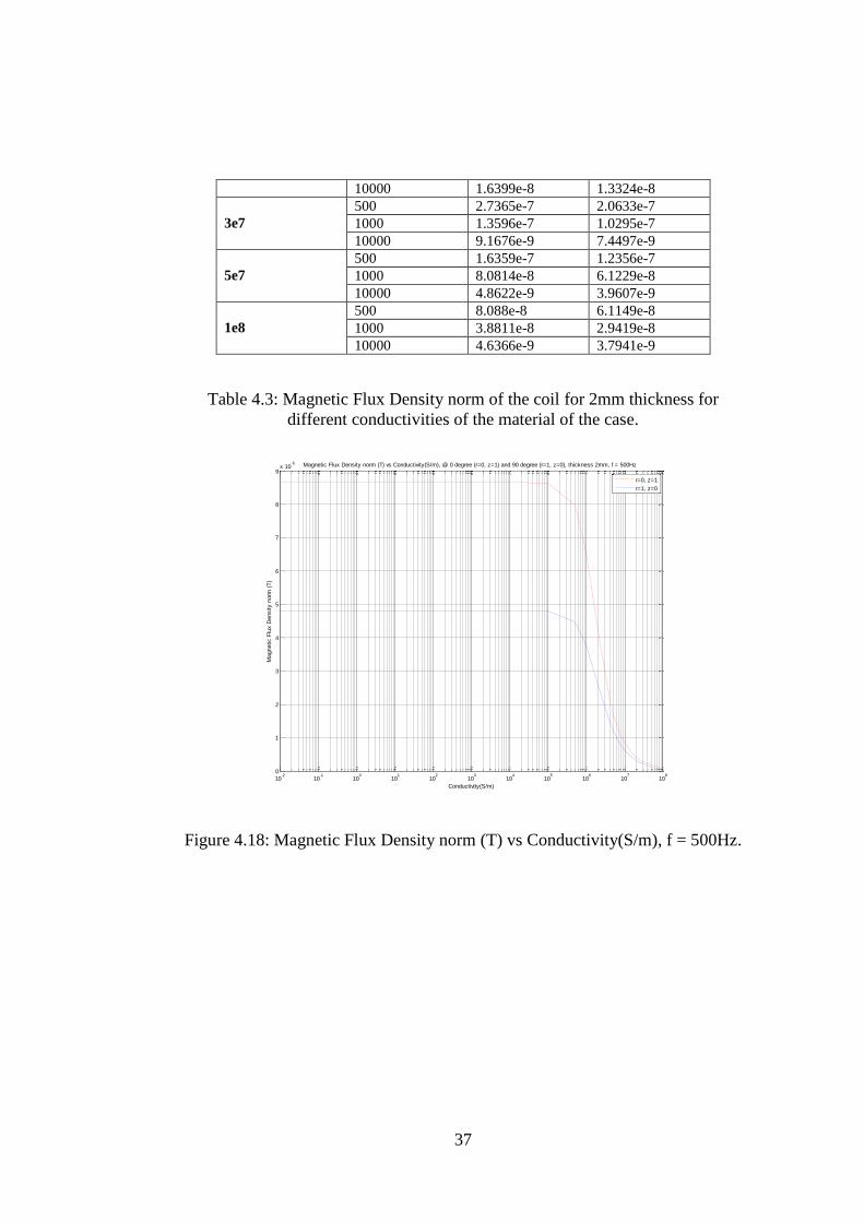
Table 4.3: Magnetic Flux Density norm of the coil for 2mm thickness for
different conductivities of the material of the case.
Figure 4.18: Magnetic Flux Density norm (T) vs Conductivity(S/m), f = 500Hz.
10-2
10-1
100
101
102
103
104
105
106
107
108
0
1
2
3
4
5
6
7
8
9x 10
-6 Magnetic Flux Density norm (T) vs Conductivity(S/m), @ 0 degree (r=0, z=1) and 90 degree (r=1, z=0), thickness 2mm, f = 500Hz
Conductivity(S/m)
Magnetic F
lux D
ensity n
orm
(T
)
r=0, z=1
r=1, z=0

38
Figure 4.19 : Magnetic Flux Density norm (T) vs Conductivity(S/m), f =
10000Hz.
Secondly, we repeat the calculations for 1mm thickness of the case.
Case material Conductivity(
S/m) @ 200C
Frequency
(Hz)
Magnetic Flux Density norm
(T)
r=0, z=1m r=1m, z=0
Copper(Cu)
5.96 x 10⁷
500 2.7633e-7 2.0751e-7
1000 1.3768e-7 1.0383e-7
10000 1.1955e-8 9.6731e-9
Aluminum
(Al)
3.50 x 10⁷
500 4.7204e-7 3.5299e-7
1000 2.3493e-7 1.7692e-7
10000 2.1909e-8 1.7725e-8
Stainless Steel
1.45 x 10⁶
500 7.3653e-6 4.1575e-6
1000 5.3462e-6 3.1647e-6
10000 5.564e-7 4.4532e-7
Carbon
(perpendicular
to base plane)
2 to 3x 10⁵
500 8.6117e-6 4.7734e-6
1000 8.4663e-6 4.7116e-6
10000 3.3707e-6 2.2997e-6
Carbon (parallel
to base plane)
3.3x 10²
500 8.6594e-6 4.797e-6
1000 8.653e-6 4.8041e-6
10000 8.4488e-6 5.0417e-6
Table 4.4: Magnetic Flux Density norm for 1mm thickness for different
materials.
10-2
10-1
100
101
102
103
104
105
106
107
108
0
1
2
3
4
5
6
7
8
9x 10
-6
Conductivity(S/m)
Magnetic F
lux D
ensity n
orm
(T
)
Magnetic Flux Density norm (T) vs Conductivity(S/m), @ 0 degree (r=0, z=1) and 90 degree (r=1, z=0), thickness 2mm, f = 10000Hz
r=0, z=1
r=1, z=0

39
Conductivity(S/m) Frequency (Hz) Magnetic Flux Density norm (T)
r=0, z=1m
r=1m, z=0
0.01
500 8.6594e-6 4.797e-6
1000 8.653e-6 4.8041e-6
10000 8.4488e-6 5.0418e-6
0.1
500 8.6594e-6 4.797e-6
1000 8.653e-6 4.8041e-6
10000 8.4488e-6 5.0418e-6
1
500 8.6594e-6 4.797e-6
1000 8.653e-6 4.8041e-6
10000 8.4488e-6 5.0418e-6
10
500 8.6594e-6 4.797e-6
1000 8.653e-6 4.8041e-6
10000 8.4488e-6 5.0418e-6
1e2
500 8.6594e-6 4.797e-6
1000 8.653e-6 4.8041e-6
10000 8.4488e-6 5.0418e-6
1e3
500 8.6594e-6 4.797e-6
1000 8.653e-6 4.8041e-6
10000 8.4484e-6 5.0415e-6
1e4
500 8.6593e-6 4.797e-6
1000 8.6527e-6 4.8039e-6
10000 8.4175e-6 5.0248e-6
1e5
500 8.6517e-6 4.7932e-6
1000 8.6223e-6 4.7889e-6
10000 6.405e-6 3.95e-6
5e5
500 8.4727e-6 4.7047e-6
1000 7.9667e-6 4.4641e-6
10000 1.6664e-6 1.2588e-6
1e6
500 7.9727e-6 4.4575e-6
1000 6.5578e-6 3.7667e-6
10000 8.1181e-7 6.4367e-7
2e6
500 6.5622e-6 3.7609e-6
1000 4.1979e-6 2.5852e-6
10000 4.0207e-7 3.2319e-7
3.5e6
500 4.6763e-6 2.8225e-6
1000 2.4687e-6 1.6601e-6
10000 2.2895e-7 1.8472e-7
5e6
500 3.4433e-6 2.1888e-6
1000 1.7025e-6 1.2022e-6
10000 1.6001e-7 1.2925e-7
8e6
500 2.1512e-6 1.4727e-6
1000 1.0446e-6 7.6636e-7
10000 9.9781e-8 8.0663e-8
1e7
500 1.7034e-6 1.2003e-6
1000 8.3136e-7 6.1573e-7
10000 7.9703e-8 6.4447e-8
1.5e7
500 1.1171e-6 8.1485e-7
1000 5.5109e-7 4.1209e-7
10000 5.2889e-8 4.2777e-8
2e7
500 8.319e-7 6.1483e-7
1000 4.1232e-7 3.0943e-7

40
10000 3.9423e-8 3.189e-8
3e7
500 5.5148e-7 4.1151e-7
1000 2.7426e-7 2.064e-7
10000 2.5839e-8 2.0904e-8
5e7
500 3.2966e-7 2.4731e-7
1000 1.6423e-7 1.238e-7
10000 1.4719e-8 1.1909e-8
1e8
500 1.6436e-7 1.2364e-7
1000 8.1828e-8 6.1742e-8
10000 6.0143e-9 4.8667e-9
Table 4.5: Magnetic Flux Density norm of the coil for 1mm thickness for
different conductivities of the material of the case.
Figure 4.20: Magnetic Flux Density Norm (T) vs Conductivity(S/m), f = 500Hz.
10-2
10-1
100
101
102
103
104
105
106
107
108
0
1
2
3
4
5
6
7
8
9x 10
-6 Magnetic Flux Density norm (T) vs Conductivity(S/m), @ 0 degree (r=0, z=1) and 90 degree (r=1, z=0), thickness 1mm, f = 500Hz
Conductivity(S/m)
Magnetic F
lux D
ensity n
orm
(T
)
r=0, z=1
r=1, z=0

41
Figure 4.21: Magnetic Flux Density Norm (T) vs Conductivity(S/m), f =
10000Hz.
Figure 4.22: Effect of thickness @ 0
0 (r=0, z=1).
10-2
10-1
100
101
102
103
104
105
106
107
108
0
1
2
3
4
5
6
7
8
9x 10
-6
Conductivity(S/m)
Magnetic F
lux D
ensity n
orm
(T
)
Magnetic Flux Density norm (T) vs Conductivity(S/m), @ 0 degree (r=0, z=1) and 90 degree (r=1, z=0), thickness 1mm, f = 10000Hz
r=0, z=1
r=1, z=0
10-2
10-1
100
101
102
103
104
105
106
107
108
0
1
2
3
4
5
6
7
8
9x 10
-6 Magnetic Flux Density norm (T) vs Conductivity(S/m), @ 0 degree (r=0, z=1), f = 500Hz
Conductivity(S/m)
Magnetic F
lux D
ensity n
orm
(T
)
2mm thickness
1mm thickness
42
Figure 4.23: Effect of thickness @ 900 (r=1, z=0).
We observe the effect of the electrical conductivity of the material of the case
and the effect of the thickness of the case on the magnetic flux density norm of
the coil on the two observation points for two frequencies on the preceding
figures. We observe on the Figure 4.18 to the Figure 4.23 that as the
conductivity of the material of the case increases, magnetic flux density norm of
the coil is unaffected until a certain value of the electrical conductivity in any
two frequencies. After a certain electrical conductivity value, shielding effect of
the case starts and the field attenuates rapidly. This critical value depends upon
the thickness of the case and the frequency. As can be observed on the Figure
4.18, magnetic flux density norm of the coil decreases drastically after the
conductivity exceeds 106 (S/m) when the frequency is 500Hz and the thickness
of the case is 2mm. On the other hand, as it is illustrated on the Figure 4.19
drastic attenuation of the magnetic flux density norm starts when the
conductivity of the material of the coil exceeds 104 (S/m) if the frequency is
10kHz. It can be concluded that as the frequency increases, attenuation starts for
10-2
10-1
100
101
102
103
104
105
106
107
108
0
0.5
1
1.5
2
2.5
3
3.5
4
4.5
5x 10
-6 Magnetic Flux Density norm (T) vs Conductivity(S/m), @ 90 degree (r=1, z=0), f = 500Hz
Conductivity(S/m)
Magnetic F
lux D
ensity n
orm
(T
)
2mm thickness
1mm thickness

43
lower conductivity values of the material of the case. Final observation is that as
can be seen on the Figure 4.22 and Figure 4.23 as the thickness of the case
increases, shielding effect of the case increases, magnetic flux density norm of
the coil decreases. To sum up, in order to avoid shielding effect of the material
of the case, thin and low electric conducting material must be chosen. GRP and
CRP have conductivity below 106 (S/m) and they would be good choice for the
body of an underwater system. If the body would be metal, stainless steel whose
conductivity is 1.45 x 10⁶
(S/m) would have been an ideal case.
4.3 Perturbation of the Magnetic Field Due to a
Metal Plate
In this section; we present the perturbation of the magnetic field of the coil due
to a metal plate in seawater in COMSOL Multiphysics. We study how to detect
the metal plate by measuring perturbation it creates on the magnetic flux density
of the transmitting coil. The metal plate is the target. We study the metal plate in
two cases: the material of the plate is iron and copper. We use the coil which is
presented in chapter 3 as the transmitting coil in the model. The current applied
to the coil is 1 Ampere 600Hz signal. Instead of using a receiving coil in the
model, we solve x, y and z components of the magnetic flux density of the coil
on an observation point. We investigate if the perturbations of the magnetic flux
density of the coil on the observation point are able to be measured via a
fluxgate magnetometer. We try to determine what kind of detection; in phase or
quadrature, can be done for different metals.
We take a solution medium. The solution medium is illustrated on the Figure
4.24. This is an x-directed cylinder whose radius is 100m and height is 200m.
Then, we take a target plate whose dimensions are 4cm thickness, 6m width and
12m length (0.04m x 6m x 12m).

44
Figure 4.24: Solution medium.
We put the center of the plate on the domain to the point (x=0, y=0, z=3.52m).
The plate is put parallel to x-y plane. The distance between the bottom surface
of the plate and the origin is 3.5m. The coil is at the origin (0, 0, 0). The plate
and the coil are illustrated on the Figure 4.25.

45
Figure 4.25: Coil and the metal plate.
After modeling the geometry of the coil, plate and solution domain, Magnetic
Fields interface is added under the AC/DC branch for the physics section of the
model in COMSOL Multiphysics. The equation solved in this interface is the
equation (2.12).
After adding physics for the model, we have to assign boundary conditions to
the coil, plate and outer boundary of the solution domain enclosing the coil and
plate geometries. For the coil and the solution domain enclosing the coil we
assign Ampere’s Law. The solution medium is seawater, where relative
permeability ( r) is 1, electrical conductivity (σ) is 4 (S/m) and relative
permittivity (εr) is 80. The coil domain is air, where relative permeability ( r) is
1, electrical conductivity (σ) is 0.001 (zero is not allowed by COMSOL
Multiphysics) and relative permittivity (εr) is 1. In order to validate the
accuracies of the solutions we assign electrical properties of seawater (relative
permeability ( r) 1, electrical conductivity (σ) 4 (S/m) and relative permittivity

46
(εr) 80) to the plate. Firstly we solve the magnetic flux density of the coil as if
everywhere, except coil, is seawater. Boundary condition of the surfaces of the
solution medium is magnetic insulation. The equation solved on these surfaces is
0n A . We set the tangential component of vector magnetic potential of these
boundaries to zero. In order to excite the coil, external current density is
assigned to the coil domain.
After adding physics and boundary conditions, we generate a mesh for the
model in order to discretize the geometry of the coil, plate and the solution
medium into triangular and tetrahedral elements. From Figure 4.26 to Figure
4.28 illustrate the generated meshes for the coil, plate and the solution domain.
Figure 4.26: Generated mesh of the plate coil and the solution medium.

47
Figure 4.27: Generated mesh of the plate.
Figure 4.28: Generated mesh of the coil.

48
We take an observation point with respect to the coil. The observation point is
5m away from the center of the coil in positive x direction. This point is
illustrated on the Figure 4.29.
Figure 4.29: Plate, coil and observation point.
As the last step, we add frequency domain as study step and solver sequence for
the model so as to compute the solution.
We observe the magnetic flux density of the coil through a 10cm observation
line which is centered at the observation point (x=5m, y=0, z=0). When this
observation line is x-directed (x=[4.95:5.05], y=0, z=0), y-directed (x=0, y=[-
0.05:0.05], z=0) and z-directed (x=0, y=0, z=[-0.05:0.05]), we plot x, y and z
components of the magnetic flux density of the coil through this line. We see
that the curve of x component of the field is same when the line is y and z-
directed. The slope of the y component of the field through y-directed line
equals to the slope of the z component of the field through z-directed line. We
repeat these calculations by changing the positions of the coil and the
observation point in the solution domain and have the same magnetic flux
density curves on the mentioned observation lines. These observations let us

49
validate that the coil is excited in true directions and solutions are not affected
by the position of the coil and the observation point as well as mesh of the plate.
The solution medium is big enough.

50
Figure 4.30: X component on the observation line (x=[4.95:5.05],y=0,z=0).
Figure 4.31: Y component on the observation line (x=[4.95:5.05],y=0,z=0).
Figure 4.32: Z component on the observation line (x=[4.95:5.05],y=0,z=0).

51
Figure 4.33: X component on the observation line (x=0,y=[-0.05:0.05],z=0).
Figure 4.34: Y component on the observation line (x=0,y=[-0.05:0.05],z=0).
Figure 4.35: Z component on the observation line (x=0,y=[-0.05:0.05],z=0).

52
Figure 4.36: X component on the observation line (x=0,y=0,z=[-0.05:0.05]).
Figure 4.37: Y component on the observation line (x=0,y=0,z=[-0.05:0.05]).
Figure 4.38: Z component on the observation line (x=0,y=0,z=[-0.05:0.05]).

53
Magnetic flux density of the coil at the observation point when the coil is
anywhere in the solution domain and the plate domain has electrical properties
of seawater is illustrated on the Table 4.6. We study the perturbation of these
magnetic flux density values due to eddy currents created on the metal plate.
Magnetic Flux Density (T)
x y z
6.76748e-8
-1.16503e-8i
-7.91263e-13
+4.28861e-14i
1.19563e-12
-8.4814e-14i
Table 4.6: Magnetic Flux Density of the coil on the observation point in
seawater.
The real part of the x component of the magnetic flux density of the coil is
67nT, and imaginary part is -11.6nT. We expect the y and z components of it to
be zero but there are numerical errors in the solution so they are not.
Now we start designating a detection region for the plate. Then, we study how
much the magnetic field of the coil is perturbed due to the metal plate in this
region. For a good detection performance we can restrict the amount of the
attenuation loss of the secondary fields due to eddy currents as 8.7 dB
(penetration depth) which is e-1
of magnetic flux density. Therefore, the target
has to be at most 1
0.182 e
away from the receiving sensors according to
this restriction. Wavelength (λ) of the electromagnetic wave in seawater at 600
Hz is 64m so we have to set maximum detection distance as
0.18 0.18 64 11.5m . With this assumption we take a detection region for
the plate. This region is illustrated on the Figure 4.39. According to this region;
we observe that if the transmitting coil is close to the plate with respect to z axis,
measurable perturbation of the magnetic flux density of the coil starts when the
observation point is near to the edges of the plate. However, if the coil is away
from the plate with respect to z axis, measurable perturbation of the magnetic
flux density of the coil starts when the coil comes to middle of the plate.

54
Described region is a rectangular pyramid. We designate that transmitting coil
travels from minus x to plus x. We study 22m range of the coil from x=-15m to
x=7m. We choose two paths for the coil to move; (x, y=0, z=0) and (x, y=0, z= -
3.5). We solve the perturbation as the coil moves on these paths. These paths are
3.5m and 7m away from the plate respectively with respect to z axis. As the coil
travels from x=-15m to x=7m, observation point travels from x=-10m to x=12m.
After determining the detection region, we solve the problem for the iron and
copper plate.
Figure 4.39: Plate detection range.
(0, 0, 0)
z
6m
y
12m
0.04
m
x
3.5m
3.5m

55
4.3.1 Iron Plate
Eddy currents are electric currents induced within conductors by a changing
field in the conductor, [40]. If either the conductor moves through a steady field,
or the magnetic field changes around a stationary conductor, eddy currents occur
in the conductor. The circulating eddy currents have inductance and thus induce
magnetic fields. Lenz's law governs this phenomenon. This law states that an
induced electromotive force (emf) always gives rise to a current whose magnetic
field opposes the original change in magnetic flux, [40]. Lenz's law is illustrated
with the negative sign in Faraday's law of induction. Induced emf ( ) and the
change in magnetic flux ( B ) have opposite signs, [41].
B
t
(4.1)
In our analysis, the transmitting coil which is driven by alternating current (AC)
passes under the metal plate. AC current of the coil creates changing magnetic
field and this changing field creates eddy currents on the metal plate as governed
by Lenz's law. These eddy currents oppose the original change in magnetic flux
and perturb this field. Our aim is to detect this metal plate in a certain region by
measuring the perturbation of the magnetic flux density of the coil.
We study perturbation of the magnetic flux density of the coil due to iron plate
in this section. We put the coil to the origin (0, 0, 0). Electrical properties of iron
are unit relative permittivity (ε0), 4000 relative permeability ( r) and 1.12 x 10⁷
(S/m) electrical conductivity (σ). Due to the fact that the relative permeability of
the copper is 4000, magnetic field cannot completely penetrate into the interior
of the plate. The formula of skin depth is1
( )mf
. Skin depth is about
0.1mm at 600 Hz for the iron plate. Therefore, we do not need to solve the
interior domain of the iron plate in the physics. We can solve the fields only on

56
the surfaces of the plate. Boundary condition of the six surfaces of the iron plate
is impedance boundary condition. The equation solved on the surfaces of the
plate is the following:
0
0
. .rs s
r
n H E n E n n E n E
j
. (4.2)
After adding physics and boundary conditions, we generate a mesh for the
model in order to discretize the geometry of the coil, plate and the solution
medium into triangular and tetrahedral elements. In order to see the accuracy of
the mesh of the iron plate firstly we set maximum element size of it as 32cm and
solve the problem. Then we set maximum element size of it as 16cm and solve
the problem. We take an observation line as (x=[-6:6], y=0, z=3.5) which is on
the bottom surface of the plate and plot current density norm on this line for two
mesh sizes. Thus we can compare the effect of the mesh size. As seen on the
Figure 4.40, we get more accurate solution when the maximum element size is
16cm for the iron plate.
Figure 4.40: Element size 32cm (green) and 16cm (blue).

57
Now we plot the currents on the iron plate. We vary the phase angle of the eddy
currents on the bottom surface of the iron plate from 00 to 360
0 to see how their
magnitudes change while circulating on the surface of the plate. Figure 4.41 and
Figure 4.42 are two plots of the eddy currents on the bottom surface of the plate
for 00 and 75
0 phase angles respectively. The problem on these plots is that it is
not possible to compare the magnitude of arrows of the surface current densities
for varying phase angle. Plots compare the arrows with respect to the biggest
magnitude arrow on its own angle instead of a globally referenced magnitude
arrow for all varying angles.
We want to know how much real and imaginary part of the components of the
magnetic flux density on the observation point changes as the coil moves under
the iron plate. We solve the magnetic flux density of the coil when the
observation point is at 23 locations; from x =-10m to x=12m when z=0 and z=-
3.5m. The solutions of the fields are listed on the Table 4.7. When the maximum
element size of the plate is 16cm, at each location of the coil, solution takes 6
minutes 49 seconds. There are 46 locations through the x axis on the two planes,
so total solution time for the iron plate is about 5.2 hours.
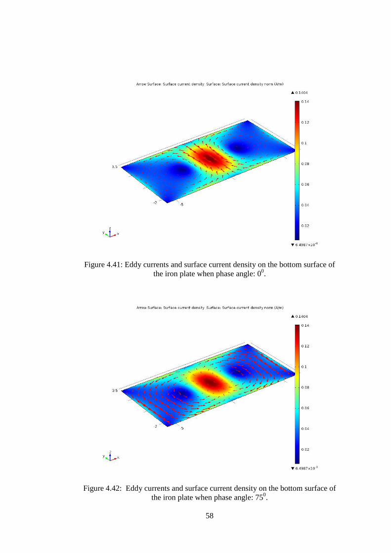
58
Figure 4.41: Eddy currents and surface current density on the bottom surface of
the iron plate when phase angle: 00.
Figure 4.42: Eddy currents and surface current density on the bottom surface of
the iron plate when phase angle: 750.

59
Iron
plate
Magnetic Flux Density (T)
Positi
on of
obser
vation
point
(x)
Path (x, y=0, z=0)
(3.5m away from the plate)
Path (x, y=0, z=-3.5)
(7m away from the plate)
x y z x y z
-10 6.76128e-8
-1.16581e-8i
1.62802e-12
-8.73932e-14i
4.50543e-11
+1.16284e-
12i
6.76349e-8-
1.16398e-8i
1.16938e-12-
6.80395e-14i
1.88278e-
11+4.79746e-
12i
-9 6.75511e-8 -1.167e-8i
9.3294e-13 -9.481e-14i
6.34747e-11 +8.69048e-
12i
6.76105e-8-1.16397e-8i
1.15034e-12-7.97215e-14i
1.53766e-11+1.30804e-
11i
-8 6.7423e-8 -1.16944e-8i
-1.58989e-13 +5.18215e-
14i
5.9582e-11 +2.16427e-
11i
6.75831e-8-1.16427e-8i
-1.19956e-12+6.62933e-
14i
6.36096e-12+2.56483e-
11i
-7 6.71864e-8 -1.17397e-8i
-6.69395e-13 -2.74946e-14i
-5.04964e-11 +4.21391e-
11i
6.75489e-8 -1.16507e-8i
-2.40652e-13 +2.26679e-
15i
-1.36744e-11 +4.31244e-
11i
-6 6.68572e-8
-1.18151e-8i
-7.96855e-13
-1.9348e-15i
-4.29991e-10
+7.29598e-11i
6.75111e-8
-1.16661e-8i
9.65619e-14
-1.8796e-14i
-5.2335e-11
+6.47391e-11i
-5 6.66239e-8
-1.19346e-8i
-6.63058e-13
-1.71031e-14i
-1.25863e-9
+1.19106e-10i
6.7483e-8
-1.16907e-8i
1.92036e-13
+4.25972e-14i
-1.05958e-10
+8.77571e-11i
-4 6.67662e-8
-1.21165e-8i
1.35265e-12
+9.22473e-
15i
-2.47446e-9
+1.73462e-10
6.74602e-8
-1.17237e-8i
2.26564e-16
+3.09046e-
15i
-1.70635e-10
+1.0815e-10i
-3 6.73703e-8
-1.23643e-8i
1.09569e-12
-9.23484e-14i
-3.76469e-9
+2.06179e-
10i
6.74529e-8
-1.17618e-8i
-1.14932e-14
+2.12841e-
14i
-2.32454e-10
+1.21529e-
10i
-2 6.81947e-8 -1.26405e-8i
-1.08316e-12 +5.14974e-
14i
-4.75523e-9 +1.80566e-
10i
6.74561e-8 -1.18002e-8i
2.35016e-13 -1.9e-14i
-2.84517e-10 +1.24751e-
10i
-1 6.88041e-8
-1.28685e-8i
-6.9344e-13
+8.77918e-
14i
-5.25071e-9
+8.52892e-
11i
6.74564e-8
-1.1833e-8i
-1.19429e-12
+6.43292e-
15i
-3.1581e-10
+1.16982e-
10i
0 6.89569e-8
-1.29842e-8i
4.85641e-13
-2.73673e-14i
-5.35762e-9
-4.80127e-11i
6.74556e-8
-1.18569e-8i
9.182e-13
+1.83699e-
14i
-3.33433e-10
+1.00172e-
10i
1 6.8823e-8 -1.30007e-8i
1.24376e-12 -3.90678e-15i
-5.3209e-9 -1.73983e-10i
6.74581e-8 -1.18717e-8i
1.06235e-13 +2.31642e-
14i
-3.36755e-10 +7.67143e-
11i
2 6.8687e-8 -1.29849e-8i
-7.18857e-13 -9.53529e-14i
-5.24905e-9 -2.81972e-10i
6.74519e-8 -1.18782e-8i
-1.10275e-12 +3.60455e-
14i
-3.29146e-10 +4.88827e-
11i
3 6.86875e-8
-1.29848e-8i
-8.61177e-14
-1.33719e-13i
-5.09603e-9
-4.00311e-10i
6.74527e-8
-1.18782e-8i
3.77186e-13
-5.46926e-14i
-3.14192e-10
+1.74793e-11i
4 6.88239e-8
-1.30006e-8i
4.51721e-13
-5.05925e-14i
-4.7236e-9
-5.7282e-10i
6.74554e-8
-1.18716e-8i
5.68954e-13
-7.52903e-14i
-2.87537e-10
-1.70575e-11i
5 6.89573e-8 -1.29838e-8i
1.15401e-13 +1.54007e-
14i
-3.9822e-9 -8.23627e-10i
6.7459e-8 -1.1857e-8i
-3.0367e-13 -2.99855e-14i
-2.50521e-10 -5.28344e-11i
6 6.88012e-8 -1.28683e-8i
-7.78538e-13 +6.62836e-
14i
-2.87833e-9 -1.11175e-9i
6.74575e-8 -1.18331e-8i
3.38665e-13 +3.91175e-
14i
-2.08279e-10 -8.57351e-11i
7 6.81959e-8
-1.26407e-8i
-2.26217e-13
-3.90064e-14i
-1.76547e-9
-1.33236e-9i
6.74543e-8
-1.18002e-8i
-1.38764e-12
-3.4301e-14i
-1.68226e-10
-1.10093e-10i
8 6.73698e-8
-1.23647e-8i
1.91772e-13
+6.45656e-
14i
-1.04197e-9
-1.39636e-9i
6.74547e-8
-1.1762e-8i
-4.46014e-13
+3.37821e-
14i
-1.38012e-10
-1.20801e-10i
9 6.67626e-8 -1.2117e-8i
-4.17305e-13 +4.51303e-
14i
-7.77081e-10 -1.27732e-9i
6.74604e-8 -1.17237e-8i
5.14914e-14 -2.72915e-14i
-1.2078e-10 -1.16173e-10i
10 6.66201e-8 -3.12154e-13 -7.40084e-10 6.74814e-8 -6.21796e-14 -1.08904e-10
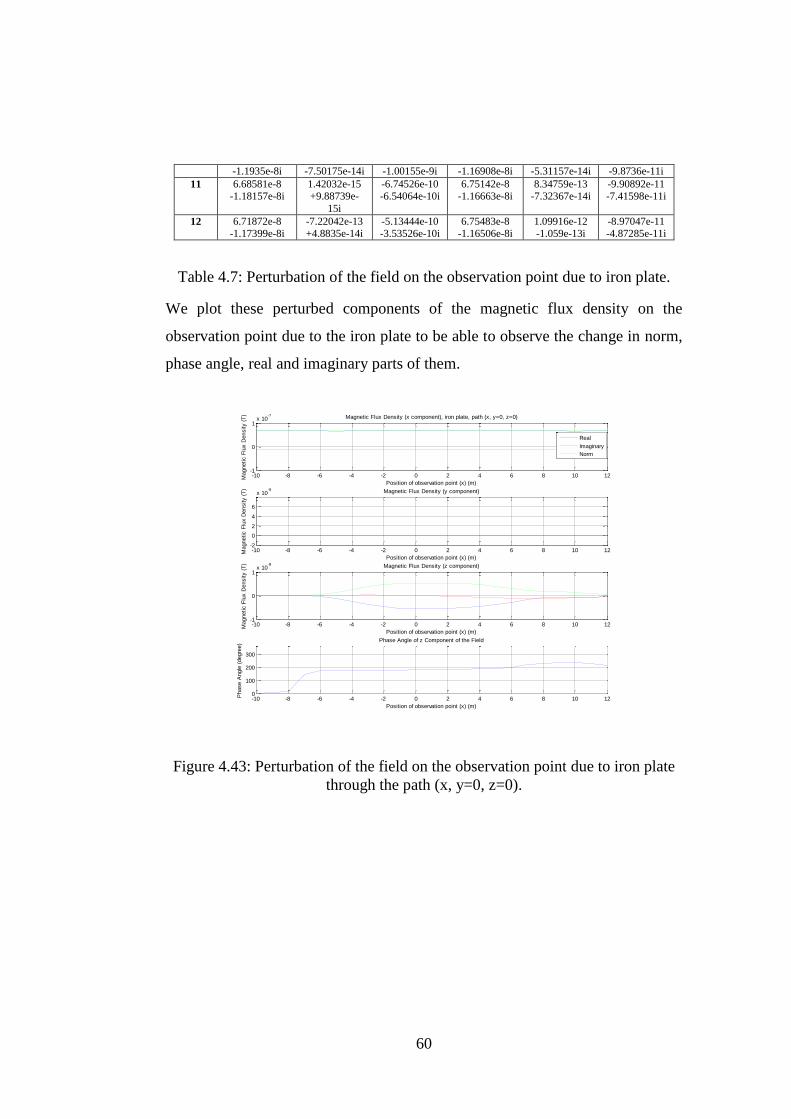
60
-1.1935e-8i -7.50175e-14i -1.00155e-9i -1.16908e-8i -5.31157e-14i -9.8736e-11i
11 6.68581e-8 -1.18157e-8i
1.42032e-15 +9.88739e-
15i
-6.74526e-10 -6.54064e-10i
6.75142e-8 -1.16663e-8i
8.34759e-13 -7.32367e-14i
-9.90892e-11 -7.41598e-11i
12 6.71872e-8 -1.17399e-8i
-7.22042e-13 +4.8835e-14i
-5.13444e-10 -3.53526e-10i
6.75483e-8 -1.16506e-8i
1.09916e-12 -1.059e-13i
-8.97047e-11 -4.87285e-11i
Table 4.7: Perturbation of the field on the observation point due to iron plate.
We plot these perturbed components of the magnetic flux density on the
observation point due to the iron plate to be able to observe the change in norm,
phase angle, real and imaginary parts of them.
Figure 4.43: Perturbation of the field on the observation point due to iron plate
through the path (x, y=0, z=0).
-10 -8 -6 -4 -2 0 2 4 6 8 10 12-1
0
1x 10
-7
Position of observation point (x) (m)
Magnetic F
lux D
ensity (
T) Magnetic Flux Density (x component), iron plate, path (x, y=0, z=0)
-10 -8 -6 -4 -2 0 2 4 6 8 10 12-2
0
2
4
6
x 10-9
Position of observation point (x) (m)
Magnetic F
lux D
ensity (
T) Magnetic Flux Density (y component)
-10 -8 -6 -4 -2 0 2 4 6 8 10 12-1
0
1x 10
-8
Position of observation point (x) (m)
Magnetic F
lux D
ensity (
T) Magnetic Flux Density (z component)
-10 -8 -6 -4 -2 0 2 4 6 8 10 120
100
200
300
Position of observation point (x) (m)
Phase A
ngle
(degre
e)
Phase Angle of z Component of the Field
Real
Imaginary
Norm

61
Figure 4.44: Perturbation of the field on the observation point due to iron plate
through the path(x, y=0, z=-3.5).
Our first observation about the preceding two plots is that change in the z
component of the magnetic flux density on the observation point is measurable
via a fluxgate magnetometer. The strength of the field is levels of nanotesla. As
the coil goes away from the iron plate with respect to z axis (from z=0 to z=-
3.5m), norm of the z component of the field decreases due to the conductivity (4
S/m) of seawater. When the observation point travels on the z=0 plane which is
3.5m away from the plate with respect to z axis, real part of the z component on
the observation point changes greater than the imaginary part of the z
component of the field. However, when the observation point travels on the z=-
3.5m plane which is 7m away from the plate with respect to z axis, imaginary
part of the z component on the observation point changes comparable amount
with respect to real part of the z component of the field. The edges of the plate
are from x=-6m to x=6m. We can observe the perturbation of the field under the
plate between these edges when we have a look at the norm of the z component
of the field. As the coil starts leaving the plate, phase angle of the z component
of the field increases. This effect can be seen around x=9m. There is symmetry
-10 -8 -6 -4 -2 0 2 4 6 8 10 12-5
0
5
10x 10
-8
Position of observation point (x) (m)
Mag
netic
Flu
x D
ensi
ty (
T) Magnetic Flux Density (x component), iron plate, path (x, y=0, z=-3.5m)
-8 -6 -4 -2 0 2 4 6 8 10 12-2
0
2
4
6
8x 10
-10
Position of observation point (x) (m)
Mag
netic
Flu
x D
ensi
ty (
T) Magnetic Flux Density (y component)
-10 -8 -6 -4 -2 0 2 4 6 8 10 12-5
0
5x 10
-10
Position of observation point (x) (m)
Mag
netic
Flu
x D
ensi
ty (
T) Magnetic Flux Density (z component)
-10 -8 -6 -4 -2 0 2 4 6 8 10 120
100
200
300
Position of observation point (x) (m)
Pha
se A
ngle
(de
gree
)
Phase Angle of z Component of the Field
Real
Imaginary
Norm

62
around y=0 plane on the geometry so y component of the magnetic flux density
on the observation point is zero.
4.3.2 Copper Plate
We solve the fields when the material of the metal plate is copper in this section.
We put the coil to the origin (0, 0, 0) again. Electrical properties of copper are
unit relative permittivity (ε0), unit relative permeability ( 0) and 5.998 x 10⁷
(S/m) electrical conductivity (σ). Due to the fact that the relative permeability of
the copper is one, magnetic field can penetrate into the interior of the plate. Skin
depth is 2.663mm at 600 Hz for copper plate. Therefore, we also need to solve
the interior domain of the copper plate. Ampere's Law is assigned to the domain
of the copper plate and material properties of the copper are assigned to this
domain.
After adding physics and boundary conditions for the copper plate like iron plate
case, we generate a mesh for the model in order to discretize the geometry of the
coil, plate and the solution medium into triangular and tetrahedral elements. We
re-generate the mesh of the plate.
In order to see the accuracy of the mesh of the copper plate firstly we set
maximum element size of it as 10cm and solve the problem. Then we set
maximum element size of it as 8cm and solve the problem. We take an
observation line as (x=[-6:6], y=0, z=3.5) which is on the bottom surface of the
plate and plot current density norm on this line for two mesh sizes. Thus we can
compare the effect of the mesh size. Comparison can be seen on the Figure 4.45.
For these two mesh sizes, solution does not change distinguishably. Increasing
mesh size gets calculations to last much longer time and causes to get warning
of "out of memory".

63
Figure 4.45: Element size 10cm (green) and 8cm (blue).
Figure 4.46: Generated mesh of the copper plate.

64
As done for the iron plate, we plot the currents on the copper plate. We vary the
phase angle of the eddy currents on the bottom surface of the copper plate from
00 to 360
0 to see how their strength changes. Figure 4.47 and Figure 4.48 are two
plots of the eddy currents on the bottom surface of the plate for 00 and 75
0
respectively. The same problem is valid also in this situation; we cannot
compare the magnitude of arrows of the surface current densities.
We want to know how much real and imaginary part of the components of the
magnetic flux density on the observation point changes as the coil moves under
the copper plate. We solve the magnetic flux density of the coil when the
observation point is at 23 locations; from x =-10m to x=12m when z=0 and z=-
3.5m. The solutions of the fields are listed on the Table 4.8. When the maximum
element size of the plate is 10cm, at each location of the coil, solution takes 10
minutes 45 seconds. There are 46 locations through the x axis on the two planes,
so total solution time for the copper plate is about 8.2 hours.

65
Figure 4.47: Eddy currents and surface current density on the bottom surface of
the copper plate when phase angle of the current: 00.
Figure 4.48: Eddy currents and surface current density on the bottom surface of
the copper plate when phase angle of the current: 750.

66
Copper
plate
Magnetic Flux Density (T)
Position of
observation
point (x)
Plane (x, y=0, z=0)
(3.5m away from the plate)
Plane (x, y=0, z=-3.5)
(7m away from the plate)
x y z x y z
-10 6.76021e-8-
1.16322e-8i
1.30773e-12-
1.54356e-13i
5.05768e-
11+1.67586e-
11i
6.7632e-8-
1.16325e-8i
1.16976e-12-
6.84117e-14i
2.15357e-
11+1.03137e-
11i
-9 6.75241e-8-1.16254e-8i
-1.74032e-12+3.17197e-
14i
6.06198e-11+2.5876e-
11i
6.7605e-8-1.16296e-8i
1.15108e-12-8.03045e-14i
1.73838e-11+2.33168e-
11i
-8 6.73668e-8-1.16232e-8i
7.06063e-13-6.13521e-15i
3.09168e-11+1.0678e-
10i
6.75741e-8-1.16298e-8i
-1.1988e-12+6.64149e-
14i
2.96942e-12+4.32058e-
11i
-7 6.7089e-8 -1.16445e-
8i
-6.97547e-13 -2.28288e-
14i
-1.56106e-10 +2.23712e-
10i
6.7536e-8 -1.16355e-
8i
-2.37657e-13 -2.99699e-
16i
-1.90357e-11 +7.10966e-
11i
-6 6.67413e-8
-1.17299e-8i
-8.0106e-13
+3.19199e-16i
-7.03368e-10
+4.14804e-10i
6.74946e-8
-1.16499e-8i
9.56329e-14
-1.69802e-14i
-6.571e-11
+1.06189e-10i
-5 6.65784e-8
-1.19292e-8i
-5.41132e-13
-3.05555e-14i
-1.78131e-9
+6.67404e-10i
6.74646e-8
-1.16756e-8i
1.91119e-13
+4.12696e-14i
-1.29818e-10
+1.44838e-10i
-4 6.69003e-8
-1.22617e-
8i
1.3657e-12
-4.58275e-
15i
-3.26005e-9
+9.35476e-
10i
6.74418e-8
-1.17116e-
8i
-3.3988e-15
+1.70945e-
15i
-2.05782e-10
+1.81334e-
10i
-3 6.77381e-8
-1.26966e-
8i
1.04811e-12
-1.15489e-
13i
-4.76727e-9
+1.16591e-9i
6.7436e-8
-1.17539e-
8i
-1.19112e-14
+1.53791e-
14i
-2.77599e-10
+2.09276e-
10i
-2 6.8758e-8 -1.31458e-
8i
-1.00877e-12 +2.0502e-14i
-5.89834e-9 +1.30721e-9i
6.74407e-8 -1.17964e-
8i
2.34914e-13 -1.36654e-
14i
-3.36913e-10 +2.23831e-
10i
-1 6.94473e-8 -1.34761e-
8i
-6.85724e-13 +1.05407e-
13i
-6.45406e-9 +1.32504e-9i
6.74415e-8 -1.18321e-
8i
-1.19155e-12 +8.91322e-
15i
-3.72461e-10 +2.23245e-
10i
0 6.95763e-8
-1.36076e-8i
6.15971e-13
-1.225e-13i
-6.57161e-9
+1.24183e-9i
6.74399e-8
-1.18573e-8i
9.19415e-13
+1.10932e-14i
-3.92126e-10
+2.095e-10i
1 6.93941e-8
-1.35995e-
8i
1.17615e-12
+2.78003e-
14i
-6.53129e-9
+1.12223e-9i
6.7441e-8
-1.18722e-
8i
1.08426e-13
+1.57367e-
14i
-3.96221e-10
+1.85564e-
10i
2 6.92309e-8
-1.35639e-8i
-5.54567e-13
-2.07555e-13i
-6.45461e-9
+9.98635e-10i
6.74339e-8
-1.18785e-8i
-1.10094e-12
+3.13612e-14i
-3.88643e-10
+1.54295e-10i
3 6.92314e-8
-1.35638e-
8i
-2.61935e-14
-1.6946e-13i
-6.29269e-9
+8.48589e-
10i
6.74347e-8
-1.18785e-
8i
3.77231e-13
-5.05491e-
14i
-3.72763e-10
+1.16697e-
10i
4 6.93949e-8
-1.35992e-
8i
4.8391e-13
-5.69511e-
14i
-5.89426e-9
+6.16906e-
10i
6.74384e-8
-1.18722e-
8i
5.68152e-13
-7.22284e-
14i
-3.43748e-10
+7.31648e-
11i
5 6.95764e-8 -1.36068e-
8i
9.00792e-14 +2.53748e-
14i
-5.07758e-9 +2.522e-10i
6.74433e-8 -1.18574e-
8i
-3.03961e-13 -3.19678e-
14i
-3.02384e-10 +2.558e-11i
6 6.94438e-8 -1.34754e-
8i
-8.52326e-13 +1.016e-13i
-3.80906e-9 -2.23197e-
10i
6.74425e-8 -1.18322e-
8i
3.37114e-13 +4.00411e-
14i
-2.5377e-10 -2.14335e-
11i
7 6.87591e-8
-1.31459e-8i
-2.63213e-13
-2.82149e-14i
-2.46356e-9
-6.69722e-10i
6.74389e-8
-1.17964e-8i
-1.38607e-12
-3.79011e-14i
-2.06139e-10
-6.09273e-11i
8 6.77378e-8
-1.26972e-8i
1.77639e-13
+6.08121e-14i
-1.52818e-9
-9.39817e-10i
6.74377e-8
-1.17541e-8i
-4.47295e-13
+3.24354e-14i
-1.68547e-10
-8.60077e-11i
9 6.68968e-8
-1.22624e-8i
-4.50082e-13
+4.8409e-14i
-1.1241e-9
-9.87624e-10i
6.7442e-8
-1.17116e-8i
5.14774e-14
-2.54015e-14i
-1.45302e-10
-9.33937e-11i
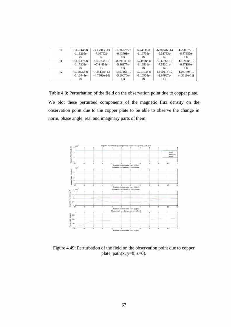
67
10 6.65744e-8 -1.19295e-
8i
-3.13809e-13 -7.05752e-
14i
-1.00269e-9 -8.43701e-
10i
6.7463e-8 -1.16756e-
8i
-6.28841e-14 -5.51783e-
14i
-1.29057e-10 -8.47356e-
11i
11 6.67417e-8
-1.17302e-8i
3.86733e-15
+7.44658e-15i
-8.6951e-10
-5.86377e-10i
6.74978e-8
-1.16501e-8i
8.34726e-13
-7.55301e-14i
-1.15998e-10
-6.57153e-11i
12 6.70895e-8
-1.16444e-8i
-7.24434e-13
+4.7568e-14i
-6.42716e-10
-3.30076e-10i
6.75353e-8
-1.16354e-8i
1.10011e-12
-1.04887e-13i
-1.03789e-10
-4.3319e-11i
Table 4.8: Perturbation of the field on the observation point due to copper plate.
We plot these perturbed components of the magnetic flux density on the
observation point due to the copper plate to be able to observe the change in
norm, phase angle, real and imaginary parts of them.
Figure 4.49: Perturbation of the field on the observation point due to copper
plate, path(x, y=0, z=0).
-10 -8 -6 -4 -2 0 2 4 6 8 10 12-5
0
5
10x 10
-8
Position of observation point (x) (m)
Magnetic F
lux D
ensity (
T) Magnetic Flux Density (x component), copper plate, path (x, y=0, z=0)
-10 -8 -6 -4 -2 0 2 4 6 8 10 12-2
0
2
4
6
x 10-9
Position of observation point (x) (m)
Magnetic F
lux D
ensity (
T) Magnetic Flux Density (y component)
-10 -8 -6 -4 -2 0 2 4 6 8 10 12-1
-0.5
0
0.5
1x 10
-8
Position of observation point (x) (m)
Magnetic F
lux D
ensity (
T) Magnetic Flux Density (z component)
-10 -8 -6 -4 -2 0 2 4 6 8 10 120
100
200
300
Position of observation point (x) (m)
Phase A
ngle
(degre
e)
Phase Angle of z Component of the Field
Real
Imaginary
Norm

68
Figure 4.50: Perturbation of the field on the observation point due to copper
plate, path(x, y=0, z=-3.5).
Our observation about the preceding two plots is that change in the z component
of the magnetic flux density on the observation point is measurable via a
fluxgate magnetometer. The strength of the field is levels of nanotesla. As the
coil goes away from the copper plate with respect to z axis (from z=0 to z=-
3.5m), norm of the z component of the field decreases due to the conductivity (4
S/m) of seawater as in the iron case. When the observation point travels on the
z=0 plane which is 3.5m away from the plate with respect to z axis, real part of
the z component of the magnetic flux density on the observation point changes
greater than the imaginary part of the z component of the field. However, when
the observation point travels on the z=-3.5m plane which is 7m away from the
plate with respect to z axis, imaginary part of the z component of the magnetic
flux density changes comparable amount with respect to real part of the z
component of the field. The edges of the plate are from x=-6m to x=6m. We can
observe the perturbation of the field under the plate between these edges when
we have a look at the norm of the z component of the field. As the coil starts
leaving the plate, phase angle of the z component of the field increases. This
-10 -8 -6 -4 -2 0 2 4 6 8 10 12-5
0
5
10x 10
-8
Position of observation point (x) (m)
Mag
netic
Flu
x D
ensi
ty (
T) Magnetic Flux Density (x component), copper plate, path (x, y=0, z=-3.5m)
-10 -8 -6 -4 -2 0 2 4 6 8 10 12-2
0
2
4
6
8x 10
-10
Position of observation point (x) (m)
Mag
netic
Flu
x D
ensi
ty (
T) Magnetic Flux Density (y component)
-10 -8 -6 -4 -2 0 2 4 6 8 10 12-5
0
5x 10
-10
Position of observation point (x) (m)
Mag
netic
Flu
x D
ensi
ty (
T) Magnetic Flux Density (z component)
-10 -8 -6 -4 -2 0 2 4 6 8 10 120
100
200
300
Position of observation point (x) (m)
Pha
se A
ngle
(de
gree
)
Phase Angle of z Component of the Field
Real
Imaginary
Norm

69
effect can be seen around x=9m. There is symmetry around y=0 plane on the
geometry so y component of the magnetic flux density on the observation point
is zero again.
We observe the perturbation of the magnetic flux density on the observation
point due to iron and copper plates on the preceding plots. In the followings we
compare and contrast the perturbation of the magnetic flux density due to iron
and copper plates on the observation points on the same plots. Electrical
properties of iron are unit relative permittivity (ε0), 4000 relative permeability (
r) and 1.12 x 10⁷ (S/m) electrical conductivity (σ). Electrical properties of
copper are unit relative permittivity (ε0), unit relative permeability ( 0) and
5.998 x 10⁷ (S/m) electrical conductivity (σ). We try to investigate the effect of
electrical conductivity and relative permeability of the plate on the perturbation
of the field on the observation point.
Figure 4.51: Perturbation of the field on the observation point (x component),
iron vs. copper through the path(x, y=0, z=0).
-10 -8 -6 -4 -2 0 2 4 6 8 10 126.6
6.8
7x 10
-8
Position of observation point (x) (m)
Mag
netic
Flu
x D
ensi
ty (
T) Magnetic Flux Density (x component), Real part, path (x, y=0, z=0)
-10 -8 -6 -4 -2 0 2 4 6 8 10 12
-1.3
-1.2
-1.1x 10
-8
Position of observation point (x) (m)
Mag
netic
Flu
x D
ensi
ty (
T) Magnetic Flux Density (x component), Imaginary part
-10 -8 -6 -4 -2 0 2 4 6 8 10 12
6.8
7
7.2x 10
-8
Position of observation point (x) (m)
Mag
netic
Flu
x D
ensi
ty (
T) Magnetic Flux Density (x component), Norm
-10 -8 -6 -4 -2 0 2 4 6 8 10 12348
349
350
351
Position of observation point (x) (m)
Pha
se A
ngle
(de
gree
)
Phase Angle (x component)
Iron plate
Copper plate

70
Figure 4.52: Perturbation of the field on the observation point (z component),
iron vs. copper through the path(x, y=0, z=0).
We observe on the preceding two plots that as the observation point moves from
the x=-10m to x=12m on z=0 plane, norm of x component of the field on the
observation point increases due to the fact that x components of the secondary
fields created by the eddy currents on the metal plate superpose onto the x
component of the magnetic flux density of the coil. Norm of z component of the
field increases more when plate is copper than when the plate is iron due to the
fact that electrical conductivity of copper (5.998 x 10⁷ (S/m)) is higher than
electrical conductivity of iron (5.998 x 10⁷ (S/m)). Difference on the phase
angles of the z components of the iron and copper plates is 14.50 when the
observation point is at x=5m and the coil is at the origin, at the middle of the
plate.
-10 -8 -6 -4 -2 0 2 4 6 8 10 12-1
0
1x 10
-8
Position of observation point (x) (m)
Magnetic
Flu
x D
ensi
ty (
T)
Magnetic Flux Density (z component), Real part, path (x, y=0, z=0)
-10 -8 -6 -4 -2 0 2 4 6 8 10 12-2
0
2x 10
-9
Position of observation point (x) (m)
Magnetic
Flu
x D
ensi
ty (
T)
Magnetic Flux Density (z component), Imaginary part
-10 -8 -6 -4 -2 0 2 4 6 8 10 120
0.5
1x 10
-8
Position of observation point (x) (m)
Magnetic
Flu
x D
ensi
ty (
T)
Magnetic Flux Density (z component), Norm
-10 -8 -6 -4 -2 0 2 4 6 8 10 120
100
200
300
Position of observation point (x) (m)
Phase
Angle
(degre
e) Phase Angle (z component)
Iron plate
Copper plate

71
Figure 4.53: Perturbation of the field on the observation point (x component),
iron vs. copper through the path(x, y=0, z=-3.5).
Figure 4.54: Perturbation of the field on the observation point (z component),
iron vs. copper through the path(x, y=0, z=-3.5).
-10 -8 -6 -4 -2 0 2 4 6 8 10 126.74
6.75
6.76
6.77x 10
-8
Position of observation point (x) (m)
Magnetic F
lux D
ensity (
T) Magnetic Flux Density (x component), Real part, path (x, y=0, z=-3.5)
-10 -8 -6 -4 -2 0 2 4 6 8 10 12-1.19
-1.18
-1.17
-1.16x 10
-8
Position of observation point (x) (m)
Magnetic F
lux D
ensity (
T) Magnetic Flux Density (x component), Imaginary part
-10 -8 -6 -4 -2 0 2 4 6 8 10 126.84
6.85
6.86
6.87x 10
-8
Position of observation point (x) (m)
Magnetic F
lux D
ensity (
T) Magnetic Flux Density (x component), Norm
-10 -8 -6 -4 -2 0 2 4 6 8 10 12350
350.1
350.2
350.3
350.4
Position of observation point (x) (m)
Phase A
ngle
(degre
e)
Phase Angle (x component)
Iron plate
Copper plate
-10 -8 -6 -4 -2 0 2 4 6 8 10 12-4
-2
0
2x 10
-10
Position of observation point (x) (m)
Mag
netic
Flu
x D
ensi
ty (
T) Magnetic Flux Density (z component), Real part, path (x, y=0, z=-3.5)
-10 -8 -6 -4 -2 0 2 4 6 8 10 12-2
0
2
4x 10
-10
Position of observation point (x) (m)
Mag
netic
Flu
x D
ensi
ty (
T) Magnetic Flux Density (z component), Imaginary part
-10 -8 -6 -4 -2 0 2 4 6 8 10 120
2
4
6x 10
-10
Position of observation point (x) (m)
Mag
netic
Flu
x D
ensi
ty (
T) Magnetic Flux Density (z component), Norm
-10 -8 -6 -4 -2 0 2 4 6 8 10 120
100
200
300
Position of observation point (x) (m)
Pha
se A
ngle
(de
gree
)
Phase Angle (z component)
Iron plate
Copper plate

72
We observe on the preceding two plots that as the observation point moves from
the x=-10m to x=12m on z=-3.5m plane, norm of x component of the field on
the observation point decreases due to the fact that x components of the
secondary fields created by the eddy currents on the metal plate superpose onto
the x component of the magnetic flux density of the coil. Norm of z component
of the field increases more when plate is copper than when the plate is iron due
to the fact that electrical conductivity of copper (5.998 x 10⁷ (S/m)) is higher
than electrical conductivity of iron (5.998 x 10⁷ (S/m)). Difference on the phase
angles of the z components of the iron and copper plates is 16.70 when the
observation point is at x=5m and the coil is at the origin, at the middle of the
plate.
We cannot barely observe the effect of relative permeability on the perturbation
of the magnetic flux density of the coil on the preceding solutions. Now we
solve the fields on the observation point (5, 0, 0) for two electrical conductivity
and relative permeability when the coil is at the origin. We solve this case like in
the copper plate; we assign ampere's law to the plate, set relative permittivity (εr)
as 1 and solve inside of it as well. The solutions are illustrated on the Table 4.9.
We cannot observe the effect of relative permeability on the phase angle of the z
component of the field. However, as the electrical conductivity changes, phase
angle of the z component of the field changes as well.
Magnetic Flux Density (T) Phase angle of z
(degree) x y z
= 5.998e7
r = 1
6.95745e-8-
1.36122e-8i
1.09891e-12-
1.08741e-14i
-5.09055e-
9+2.55984e-10i
177.12124
= 5.998e7
r = 4000
6.95746e-8-
1.36122e-8i
1.09959e-12-
1.19506e-14i
-5.09062e-
9+2.55991e-10i
177.12121
= 1.12e7
r = 4000
6.95752e-8-
1.36047e-8i
1.14818e-
12+3.37358e-
14i
-5.09342e-
9+2.41446e-10i
177.28601
= 1.12e7
r = 1
6.9574e-8-
1.36049e-8i
1.11725e-
12+5.56952e-
14i
-5.09154e-
9+2.41747e-10i
177.28163
Table 4.9: Effect of relative permeability and electrical conductivity on the
phase angle.

73
4.4 Magnetic Field Due to Current in Straight
Wire
Submarines create perturbation on the ambient Earth magnetic field due to their
ferromagnetic bodies. Magnetic anomaly detector equipped aircrafts fly over the
oceans and seas so as to detect submerged submarines. Detection performances
of MAD equipped aircrafts are tested in the development processes of these
systems. However, it is not possible to have a submerged submarine any time
tests are wanted to be done. So in order to test the performance of the MAD
equipped aircrafts, DC current carrying wire systems which create same amount
of perturbation on the ambient Earth magnetic field are developed.
In this section we designate a submarine model in a magnetic field and try to
observe how much perturbation on the field created by the submarine. Then we
designate a current carrying wire and try to observe how much magnetic field
this wire can create. We compare the perturbation on ambient Earth magnetic
field due to the submarine and magnetic field of the current carrying wire on
observation lines.
Firstly we study the perturbation of ambient Earth magnetic field due to a
submarine in COMSOL Multiphysics. As illustrated on the Figure 4.55, we take
a submarine model. Dimensions of the submarine are 60m length, 6m diameter
and 2.54cm thickness. We put this submarine into the solution medium. Solution
medium is an x-directed square prism. Dimensions of the square prism are 80m
by 80m by 200m. Solution medium and the submarine are on the Figure 4.56.

74
Figure 4.55: Model of submarine.
Figure 4.56: Submarine in the solution medium.

75
After modeling the geometry of the submarine, Magnetic Fields, No Currents
interface is added under the AC/DC branch for the physics selection of the
model. This interface solves the following equations:
. 0B , (4.3)
mH v , (4.4)
where B is the magnetic flux density vector, H is the magnetic field strength, vm
is the magnetic scalar potential.
After adding physics for the model, we assign boundary conditions to the
submarine and outer boundary of the solution domain enclosing the submarine
geometry. Boundary condition on the surfaces of the medium is magnetic
insulation. The equation solved on these surfaces is . 0n B . Boundary condition
on the surfaces of the submarine is magnetic shielding. The equation solved on
these surfaces is 1 2 0. .t r s t mn B B d V . Relative permeability of the
material of the submarine is 700. Magnetic flux density applied onto the
submarine is 50 x 10-6
(T).
After adding physics and boundary condition, we generate a mesh for the model
in order to discretize the complex geometry of the coil into triangular elements.
Generated meshes of the submarine and the solution domain can be seen on the
Figure 4.57 and Figure 4.58.

76
Figure 4.57: Generated meshes of the submarine and the solution medium.
Figure 4.58: Generated mesh of the submarine.

77
As the last step, we add stationary domain as study step and solver sequence for
the model so as to compute the solution.
We begin post-processing of the solution. We take observation lines on the
medium and observe how the magnetic field around the submarine is perturbed.
First observation line is (x=0, y=0, z=-40 to z=40). The observation line is
illustrated on the Figure 4.59. Perturbation of the magnetic field through the line
due to existence of the submarine can be seen on the Figure 4.60. Second
observation line is (x=0, y=-25 to y=25, 13). The observation line is illustrated
on the Figure 4.61. This line is 10m away from the surface of the submarine.
Perturbation of the magnetic field through the line due to existence of the
submarine can be seen on the Figure 4.62. Third observation line is (x=0, y=-25
to y=25, 18). This line is 15m away from the surface of the submarine.
Perturbation of the magnetic field through the line due to existence of the
submarine can be seen on the Figure 4.63. Forth observation line is (x=0, y=-25
to y=25, 28). This line is 25m away from the surface of the submarine.
Perturbation of the magnetic field through the line due to existence of the
submarine can be seen on the Figure 4.64.

78
Figure 4.59: Observation line (x=0, y=0, z=-40 to z=40).
Figure 4.60: Perturbation on the line of (x=0, y=0, z=-40 to z=40).

79
Figure 4.61: Observation line (x=0, y=-25 to y=25, z=13).
Figure 4.62: Perturbation on the line of (x=0, y=-25 to y=25, z=13 ). 10m above
the submarine.

80
Figure 4.63: Perturbation on the line of (x=0, y=-25 to y=25, z=18 ). 15m above
the submarine.
Figure 4.64: Perturbation on the line of (x=0, y=-25 to y=25, z=28 ). 25m above
the submarine.

81
Observation
line
(x=0, y=0, z=-
40m to 40m)
(x=0, y=-25m to
25m, z=13), 10
above surface
of submarine
(x=0, y=-25m to
25m, z=18), 15
above surface
of submarine
(x=0, y=-25m to
25m, z=28), 25
above surface
of submarine
Maximum
perturbation
(nT)
35000 2800 1400 420
Table 4.10: Perturbation of ambient Earth magnetic field due to submarine.
Secondly we study field of a current carrying wire towing system. Such current
carrying wire systems are thrown by ships or submersed submarines. They are
stand alone systems that tow the wire. The aim of these systems is to perturb
ambient Earth magnetic field like a submarine in order to test the performance
of magnetic anomaly detector equipped aircrafts.
We designate a system which tows 30m wire. The system can be seen on the
Figure 4.65. Length of 29m portion of it is insulated from the seawater and last 1
meter portion is contacting with seawater. Thus, the applied current turns back
to the tube (wire towing vehicle) 29m away from it on conducting seawater
instead of just after leaving the tube.
Figure 4.65: Current carrying wire system.
We take an x-directed cylinder as the simulation medium. The dimensions of the
cylinder are 50m radius and 100 length. We take a 30m wire. The wire and the
solution medium is shown on the Figure 4.66.

82
Figure 4.66: Wire and solution domain.
After modeling the geometry of the wire, Magnetic Fields interface is added
under the AC/DC branch for the physics selection of the model. The equation
solved in this interface is the equation (2.12).
After adding physics for the model, we need to assign boundary conditions to
the outer boundary of the solution domain enclosing the wire geometry.
Boundary conditon on the surfaces of the solution domain is magnetic
insulation. The equation solved on these surfaces is 0n A . Edge current of
8.25 Ampere is applied to the wire.
After adding physics and boundary conditions, we generate a mesh for the
model in order to discretize the complex geometry into triangular and
tetrahedral elements. In order to be able to mesh the wire well, we take a
cylinder whose radius is 0.02m. The meshing of the solution domain and the
wire are shown on the Figure 4.67.

83
Figure 4.67: Generated meshes of the wire and the solution domain.
For the final step, we have to add study and solver sequence for the model in
order to compute the solution. We add stationary domain as study step and
solver sequence for the model so as to compute the solution.
We begin post-processing of the solution. We observe fields of the wire on
different observation lines as in the submarine case. First observation line of the
magnetic flux density norm is (x=0, y=0, z=-40 to z=40). This line can be seen
on the Figure 4.68. Magnetic flux density norm along this observation line can
be seen on the Figure 4.69. Second observation line of the magnetic flux density
norm is (x=0, y=-25 to y=25, z=10). This line is illustrated on the Figure 4.70.
Magnetic flux density norm along this observation line can be seen on the
Figure 4.71. Third observation line of the magnetic flux density norm is (x=0,
y=-25 to y=25, z=15). Magnetic flux density norm along this observation line
can be seen on the Figure 4.72. Forth observation line of the magnetic flux
density norm is (x=0, y=-25 to y=25, z=25). Magnetic flux density norm along
this observation line can be seen on the Figure 4.73.
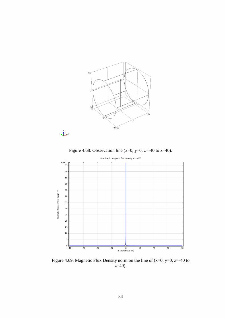
84
Figure 4.68: Observation line (x=0, y=0, z=-40 to z=40).
Figure 4.69: Magnetic Flux Density norm on the line of (x=0, y=0, z=-40 to
z=40).

85
Figure 4.70: Observation line (x=0, y=-25 to y=25, z=10).
Figure 4.71: Magnetic Flux Density norm on the line of (x=0, y=-25 to y=25,
z=10).

86
Figure 4.72: Magnetic Flux Density norm on the line of (x=0, y=-25 to y=25,
z=15).
Figure 4.73: Magnetic Flux Density norm on the line of (x=0, y=-25 to y=25,
z=25).

87
Observation
line
(x=0, y=0, z=-
40m to 40m)
(x=0, y=-25m to
25m, z=10)
(x=0, y=-25m to
25m, z=15)
(x=0, y=-25m to
25m, z=25)
Maximum
magnetic
field (nT)
650000 38 21 10
Table 4.11: Magnetic field of current carrying wire.
When we compare the perturbation of ambient Earth magnetic field due to the
submarine as well as magnetic field of the current carrying wire, we see that the
wire cannot create as much magnetic field values as on the equal distances away
from them. For instance, submarine perturbs 420nT on the observation point
(x=0, y=0, z=28m) which is 25m away from on the z-direction, but the current
of the wire creates 10nT field on the observaion point (x=0, y=0, z=25m). After
this observation, we can say that for this geometry of the wire (30m) and the
current value (8.25A), this wire cannot create as much field as the submarine
perturbs on the ambient Earth magnetic field on the same observation points.
One possible solution to this problem is that the wire can be driven by higher
current values and the observation lines of it can be closer compared to the
observation lines of the submarine. As an example, if the current on the wire is
82.5A which is ten times designated and the observation point is (x=0, y=0,
z=10m), magnetic flux density on this point is 380nT. This much perturbation
values for the submarine (420nT) can be observed when the observation point of
the submarine is (x=0, y=0, z=25) which is 25m away from it. This means that
detection performance of the magnetic anomaly detector equipped aircrafts can
be evaluated via current carrying wire systems.

88
Chapter 5
DISCUSSION & CONCLUSION
In this thesis, we focused on low frequency magnetic field in seawater. We
stated the governing equations of electromagnetic waves. We compared
electrical properties (electrical conductivity, relative permeability and relative
permittivity) of air (vacuum) and seawater. Then we compared the speed and
wavelength of electromagnetic wave in air and seawater. In order to solve
magnetic field of a coil in seawater with the help of COMSOL Multiphysics
packet software, we designed an air-cored multilayer coil which can be realized
and driven by plausible power values. After the design of the coil, we studied
low frequency magnetic field of this coil in seawater in different cases. In each
simulation, geometry of the model is taken, appropriate physics for the analysis
is chosen, boundary conditions for the geometry and enclosing solution domain
are assigned and mesh of the geometries and the medium are generated. In the
first study we solved magnetic field of the coil for three frequencies in air and in
seawater on different observation arcs, lines and points. We observed the
attenuation of magnetic field due to the electrical conductivity (4 S/m) of
seawater and due to the increase of the frequency. In the second study, we
observed the shielding effect of the electrical conductivity of the material and
thickness of the case which holds the coil. We observed that as the electrical
conductivity of the material and the thickness of the case increases, shielding of
the case on the magnetic field of the coil increases, magnetic field of the coil
attenuates more. We suggested GRP or CRP whose electrical conductivities are
under 106(S/m) for the material of the case. However, if the case has to be metal,
we suggested stainless steel whose electrical conductivity is 1.45x10⁶ (S/m). The
case has to be as thin as possible to avoid the attenuation of the field. In the third

89
study, we solved the magnetic flux density of the coil on observation points
when there is a metal plate in the medium. We designated a detection region for
the metal plate. We moved the coil and the observation point according to this
region to observe the fields on the observation point. We took the material of the
plate as iron and copper. Both of these materials have high electrical
conductivity but copper has higher electrical conductivity (5.998 x 10⁷
(S/m))
than iron (1.12 x 10⁷
(S/m)). Iron has 4000 relative permeability and copper has
unit relative permeability. Skin depth on the iron plate is 0.1mm so it was not
necessary to solve inside of it. On the other hand, skin depth on the copper plate
is 2.665mm, so it was necessary to solve inside of it. However, thickness of the
plate is so small (0.04m) compared to other edges of it (6m x 12m) and this
makes harder to generate mesh inside of the copper plate. When we wanted to
have finer meshes inside of the copper plate, we get the warning of "out of
memory". Real and imaginary parts of x and z components of the field change
due to eddy currents on the metal plate. Norm of x and z components of the
fields increases more when the plate is copper than the plate is iron. As the
electrical conductivity of the material of the plate increases, more eddy currents
are created on the metal plate, perturbation of the magnetic field on the
observation point increases as well. Change in the real part of x component of
the field occurs on 67nT, so the sensing circuit can be saturated. Change in the
imaginary part of x component of the field occurs on 1nT, so this value must be
subtracted from the measured field on the observation point to find the change in
the field. Change in the real and imaginary part of z component of the field
occurs on zero nT, so the sensing circuit cannot be saturated easily. Levels of the
perturbation of the magnetic field on the observation point due to metal plate are
between 0.3 to 10nT. Fluxgate magnetometers can measure fields of
approximately 0.1nT. This means that we can place a fluxgate magnetometer
onto the observation point to measure perturbation of the field and detect the
metal plate in the defined detection region in 7m. Difference of the phase angle
of z component of field due to iron and copper plate is around 150. This angle
can be valuable to discriminate the sort of the metal to be detected. Therefore,

90
quadrature sensing can still be useful. In the forth study, we solved the
perturbation of ambient Earth magnetic field due to a submarine as well as
solved the magnetic field of a DC current carrying wire. We investigated how
the perturbation on ambient Earth magnetic field due to the submarine can be
imitated by an underwater system which tows a DC current carrying wire. We
concluded that by applying higher DC current than 8.25A to the straight wire
and flying the magnetic anomaly detector (MAD) equipped aircraft closer to the
wire system, same levels of perturbation can be measured as levels of
perturbation due to the submerged submarine.
As a future work, a theoretical way to solve fields and currents inside of the
copper plate without meshing and solving inside of it can be studied. This can be
a boundary condition like impedance boundary condition. By just assigning this
boundary condition onto the surfaces of the copper plate and setting the
thickness of it, fields and currents can be solved inside of it with less generation
of mesh; which means that less computation power and physical memory of the
computer are required.

91
Bibliography
[1] A. Palmeiro, M. Martin, I. Crowther, and M. Rhodes, "Underwater
radio frequency communications," in OCEANS, 2011 IEEE-Spain, pp.
1-8, IEEE, 2011.
[2] M. Stojanovic, "Recent advances in high-speed underwater acoustic
communications," IEEE Journal of Oceanic Engineering, vol. 21, no.
2, pp. 125-136, 1996.
[3] R. Coates and P. Willison, "Underwater Acoustic Communications: A
Review and Bibliography," The Institute of Acoustics, 1987.
[4] R. Coates, R. Owen, and M. Zheng, "Underwater Acoustic
Communica-tions: A Review and Bibliography (ii)," PROCEEDINGS-
INSTITUTE OF ACOUSTICS, vol. 15, pp. 1-1, 1993.
[5] J. A. Catipovic, "Performance limitations in underwater acoustic
telemetry," IEEE Journal of Oceanic Engineering, vol. 15, no. 3, pp.
205-216, 1990.
[6] J. Smart, "Underwater optical communications systems Part 1:
variability of water optical parameters," in Military Communications
Conference, 2005. MILCOM 2005. IEEE, pp. 1140-1146, 2005.
[7] J. W. Giles and I. N. Bankman, "Underwater optical communications
systems. Part 2: basic design considerations," in Military
Communications Conference, 2005. MILCOM 2005. IEEE, pp. 1700-
1705, 2005.

92
[8] F. Hanson and S. Radic, "High bandwidth underwater optical
communication," Applied optics, vol. 47, no. 2, pp. 277-283, 2008.
[9] N.Farr, A. Bowen, J. Ware, C. Pontbriand, and M. Tivey, "An
integrated, underwater optical/acoustic communications system," in
OCEANS 2010 IEEE-Sydney, pp. 1-6, 2010.
[10] M. R. Frater, M. J. Ryan, and R. M. Dunbar, "Electromagnetic
communications within swarms of autonomous underwater vehicles,"
in Proceedings of the 1st ACM international workshop on Underwater
networks, pp. 64-70, ACM, 2006.
[11] X.Che, I. Wells, G. Dickers, P. Kear, and X. Gong, "Re-evaluation of
RF electromagnetic communication in underwater sensor networks,"
Communications Magazine, IEEE, vol. 48, no. 12, pp. 143-151, 2010.
[12] X.Che, I. Wells, P. Kear, G. Dickers, X. Gong, and M. Rhodes, "A
static multi-hop underwater wireless sensor network using RF
electromagnetic communications," in 29th IEEE International
Conference on Distributed Computing Systems Workshops, 2009.
ICDCS Workshops' 09., pp. 460-463, 2009.
[13] M. Rhodes, "Underwater electromagnetic propagation: re-evaluating
wireless capabilities," Hydro International, vol. 10, no. 10, pp. 28-31,
2006
[14] E. Foster, "A Diver-Operated Underwater Metal Detector,"
Archaeometry, vol. 12, no. 2, pp. 161-166, 1970.
[15] J. N. Green, E. Hall, and M. Katzev, "Survey of a Greek shipwreck o
Kyrenia, Cyprus," Archaeometry, vol. 10, no. 1, pp. 47-56, 1967.
[16] P. Czipott and W. Podney, "Use of a superconductive gradiometer in an
ultrasensitive electromagnetic metal detector," IEEE Transactions on
Magnetics, vol. 25, no. 2, pp. 1204-1207, 1989.

93
[17] C. J. Clausen and J. B. Arnold, "The magnetometer and underwater
archaeology," International Journal of Nautical Archaeology, vol. 5,
no. 2, pp. 159- 169, 1976.
[18] J. N. Heine, "Scientific diving techniques," Marine Technology Society
Journal, vol. 34, no. 4, pp. 23-37, 2001.
[19] K. Asakawa, Y. Shirasaki, and Y. Iwamoto, "Metal detector for tracing
submarine telecommunication cables," IEEE Transactions on
Instrumentation and Measurement, vol. 32, no. 4, pp. 477-483, 1983.
[20] J.-G. Webster, The Measurement, Instrumentation, and Sensors:
Handbook. Springer, 1999.
[21] D. Guelle, Metal Detector Handbook for Humanitarian Demining: A
Book about Metal Detectors, Covering Detection Procedures in the
Field, and the Testing and Evaluation of Metal Detectors for
Humanitarian Demining. Office for Offcial Publications of the
European Communities, 2003.
[22] J. Tyson, "How metal detectors work," How Stuff Works, 2003.
[23] M. Rowan and W. Lahr, "How Metal Detectors Work," 2002.
[24] V. Aravinthan and T. Nanyakkara, "Intellligent signal classification in
VLF metal detectors to distinguish landmines from harmless metal
debris," proceedings of the annual sessions of the IEE Sri Lunka
section, 2004.
[25] M. S. Sharawi and M. Sharawi, "Design and implementation of a low
cost VLF metal detector with metal-type discrimination capabilities," in
IEEE International Conference on Signal Processing and
Communications, 2007. ICSPC 2007., pp. 480-483, 2007.
[26] J. Corbyn, "Pulse induction metal detector," Wireless World, vol. 86,
no. 1531, pp. 40-44, 1980.

94
[27] W. E. Lahr, "Pulse induction metal detector," May 9 1995. US Patent
5,414,411.
[28] W.-S. Hua, J. R. Hooks, W.-J. Wu, and W.-C. Wang, "Development of
a novel polymeric fiber-optic magnetostrictive metal detector," in SPIE
Smart Structures and Materials+ Nondestructive Evaluation and
Health Monitoring, pp. 76501P-76501P, International Society for
Optics and Photonics, 2010.
[29] H. Huang and I. Won, "Characterization of UXO-like targets using
broadband electromagnetic induction sensors," IEEE Transactions on
Geoscience and Remote Sensing, vol. 41, no. 3, pp. 652-663, 2003.
[30] I. Won, S. Norton, B. SanFilipo, and F. Kunak, "Active broadband
electromagnetic detection and classification of buried naval mines," in
OCEANS'02 MTS/IEEE, vol. 2, pp. 966-973, 2002.
[31] Y. Iwamoto, Y. Shirasaki, and K. Asakawa, "Fiber-optic-tethered
unmanned submersible for searching submarine cables," in OCEANS
82, pp. 65-72, 1982.
[32] F. Primdahl, "The fluxgate magnetometer," Journal of Physics E:
Scientific Instruments, vol. 12, no. 4, p. 241, 1979.
[33] H. C. Hayes, "Detection of submarines," Proceedings of the American
Philosophical Society, vol. 59, no. 1, pp. 1-47, 1920.
[34] A. Sheinker, B. Ginzburg, N. Salomonski, P. A. Dickstein, L. Frumkis,
and B. Kaplan, "Magnetic Anomaly Detection Using High-Order
Crossing Method," IEEE Transactions on Geoscience and Remote
Sensing, vol. 50, no. 4, pp. 1095-1103, 2012.
[35] T. A. Gardner, "Magnetic Anomaly Detection." http://www.uboat.net.,
Accessed: 2013-09-02.
[36] C. Multiphysics, "4.2 User’s Guide," 2011.

95
[37] A. I. Al-Shamma'a, A. Shaw, and S. Saman, "Propagation of
electromagnetic waves at MHZ frequencies through seawater," IEEE
Transactions on Antennas and Propagation, vol. 52, no. 11, pp. 2843-
2849, 2004.
[38] H. A. Wheeler, "Simple inductance formulas for radio coils,"
Proceedings of the Institute of Radio Engineers, vol. 16, no. 10, pp.
1398-1400, 1928.
[39] C. Multiphysics, "Rf module user's guide," 2008.
[40] R. L. Stoll, The analysis of eddy currents. Clarendon Press Oxford,
1974.
[41] D. C. Giancoli and J. J. Boyle, Physics: principles with applications.
Pearson Education, 2005.

96
Appendix A
Detailed Description of Simulation:
Iron Plate
We presented solutions of perturbation of magnetic flux density of the coil
due to iron plate in the section 4.3.1. Now we present how we setup models,
boundary conditions and meshes in Comsol Multiphysics. We used Comsol
4.3a for the simulations. We solve the problem when the coil is at the origin
(0, 0, 0) and the observation point is at the point (5, 0, 0). We present this
solution as an .mph file. The name of the file is iron_35m.mph.
Firstly we selected 3D space dimension. We added physics, interface of
Magnetic Fields (mf) under AC/DC branch. We selected Frequency Domain
as the study type and started creating the models.
Under the Global Definitions branch we defined four parameters: shift_x,
shift_y, shift_z and ang to be able to parametrize the solutions. First three
parameters let us change the position of the coil and ang lets us change the
phase angle of the solution.
Under the Geometry1 branch we created solution domain which is Cylinder1
(cyl1), coil which is under the branch of Work Plane1 (wp1), plate which is
Block1 (blk1). In order to be able to solve the field more accurately on the
observation point which is 5m away from the center of the coil we created a
cylinder which Cylinder2 (cyl2) and a point which is Point1 (pt1). This
cylinder lets finer meshes be generated around the observation point. The
point lets a node of the mesh be on the observation point. Domain 1 refers to
solution domain, Domain 2 refers to plate domain, Domain 3 refers to coil

97
domain and Domain 4 refers to the cylinder which includes the observation
point.
Under the Magnetic Fields (mf) branch we assigned Ampere's Law and
boundary conditions to the model. We excluded Domain 2 from Magnetic
Fields (mf), thus we do not solve inside of it. We assigned Ampere's Law 1
to Domain 1 and Domain 4. Domain 2 is not applicable to this solution. We
set electrical conductivity ( ) to 4, relative permittivity ( r ) to 80 and
relative permeability ( r ) to 1. We created Ampere's Law 2 and assigned
Domain 3 in it. We set electrical conductivity ( ) to 0.001 (Comsol does
not let it be zero), relative permittivity ( r ) to 1 and relative permeability (
r ) to 1. Finally we assigned Impedance Boundary Condition 1 to six
surfaces of the plate. We set electrical conductivity ( ) to 1.12e7, relative
permittivity ( r ) to 1 and relative permeability ( r ) to 4000. These
electrical properties belong to iron (Fe). We assigned External Current
Density 1 to Domain 3.
Under the Mesh1 branch we set mesh parameters of the domains. We created
four Free Tetrahedral. Free Tetrahedral 2 is assigned to Domain 3 and
maximum element size is set to 4cm. Free Tetrahedral 3 is assigned to
Domain 4 and maximum element size is set to 1cm. Free Tetrahedral 4 is
assigned to Domain 2 and maximum element size is set to 16cm. Free
Tetrahedral 4 is assigned to entire geometry and predefined configuration of
Extra Fine is set.
Finally, under the Study1 branch we set the frequency and solvers. We set
600 Hz in Step1: Frequency Domain and compute.
We solved magnetic flux density on the observation point for 46 different
positions of the coil. We sweep the coil from x=-15m to x=7m on two
planes; z=0 and z=-3.5m. We added Parametric Sweep under Study 1 and
made shift_x increase from -15 to 7 when shift_z is 0 to have 23 solutions.
We repeat this process when shift_z is -3.5m and thus we have 46 solutions
for different positions of the coil under the iron plate.

98
Appendix B
Detailed Description of Simulation:
Copper Plate
We presented solutions of perturbation of magnetic flux density of the coil
due to copper plate in the section 4.3.2. Now we present how we setup
models, boundary conditions and meshes in Comsol Multiphysics. We used
Comsol 4.3a for the simulations. We solve the problem when the coil is at
the origin (0, 0, 0) and the observation point is at the point (5, 0, 0). We
present this solution as an .mph file. The name of the file is
copper_35m.mph.
Firstly we selected 3D space dimension. We added physics, interface of
Magnetic Fields (mf) under AC/DC branch. We selected Frequency Domain
as the study type and started creating the models.
Under the Global Definitions branch we defined four parameters: shift_x,
shift_y, shift_z and ang to be able to parametrize the solutions. First three
parameters let us change the position of the coil and ang lets us change the
phase angle of the solution.
Under the Geometry1 branch we created solution domain which is Cylinder1
(cyl1), coil which is under the branch of Work Plane1 (wp1), plate which is
Block1 (blk1). In order to be able to solve the field more accurately on the
observation point which is 5m away from the center of the coil we created a
cylinder which Cylinder2 (cyl2) and a point which is Point1 (pt1). This
cylinder lets finer meshes be generated around the observation point. The
point lets a node of the mesh be on the observation point. Domain 1 refers to
solution domain, Domain 2 refers to plate domain, Domain 3 refers to coil

99
domain and Domain 4 refers to the cylinder which includes the observation
point.
Under the Materials branch, we added Copper (mat1) and assigned Domain
2 in it. Thus we set the properties of the plate as Copper (Cu).
Under the Magnetic Fields (mf) branch we assigned Ampere's Law and
boundary conditions to the model. We assigned Ampere's Law 1 to Domain
1 and Domain 4. We set electrical conductivity ( ) to 4, relative
permittivity ( r ) to 80 and relative permeability ( r ) to 1. We created
Ampere's Law 2 and assigned Domain 3 in it. We set electrical conductivity (
) to 0.001 (Comsol does not let it be zero), relative permittivity ( r ) to 1
and relative permeability ( r ) to 1. We created Ampere's Law3 and
assigned Domain 2 in it. This plate domain gets electrical properties From
material. We assigned External Current Density 1 to Domain 3.
Under the Mesh1 branch we set mesh parameters of the domains. We created
four Free Tetrahedral. Free Tetrahedral 2 is assigned to Domain 3 and
maximum element size is set to 4cm. Free Tetrahedral 3 is assigned to
Domain 4 and maximum element size is set to 1cm. Free Tetrahedral 4 is
assigned to Domain 2 and maximum element size is set to 10cm. Free
Tetrahedral 4 is assigned to entire geometry and predefined configuration of
Extra Fine is set.
Finally, under the Study1 branch we set the frequency and solvers. We set
600 Hz in Step1: Frequency Domain and compute.
We solved magnetic flux density on the observation point for 46 different
positions of the coil. We sweep the coil from x=-15m to x=7m on two
planes; z=0 and z=-3.5m. We added Parametric Sweep under Study 1 and
made shift_x increase from -15 to 7 when shift_z is 0 to have 23 solutions.
We repeat this process when shift_z is -3.5m and thus we have 46 solutions
for different positions of the coil under the copper plate.