Embed Size (px)
Citation preview
UP AND DOWN CREDIT RISK
Tomasz R. Bielecki ∗
Department of Applied MathematicsIllinois Institute of Technology
Chicago, IL 60616, USA
Stephane Crepey∗
Departement de MathematiquesUniversite d’Evry Val d’Essonne
91025 Evry Cedex, France
Monique Jeanblanc†
Departement de MathematiquesUniversite d’Evry Val d’Essonne
91025 Evry Cedex, Franceand
Europlace Institute of Finance
November 7, 2008
Abstract
This paper discusses the main modeling approaches that have been developed so far for handling port-folio credit derivatives. In particular the so called top, top down and bottom up approaches are considered.We first provide an overview of these approaches. We give some mathematical insights to the fact that in-formation, namely, the choice of a relevant model filtration, is the major modeling issue. In this regard, weexamine the notion of thinning that was recently advocated for the purpose of hedging a multi-name deriva-tive by single-name derivatives. We then give a further analysis of the various approaches using simplemodels, discussing in each case the issue of hedging. Finally we explain by means of numerical simula-tions (semi-static hedging experiments) why and when the portfolio loss process may not be a sufficientstatistics for the purpose of valuation and hedging of portfolio credit risk.
∗The research of T.R. Bielecki was supported by NSF Grant 0604789.†The research of S. Crepey and M. Jeanblanc benefited from the support of the ‘Chaire Risque de credit’, Federation Bancaire
Francaise, and of the Europlace Institute of Finance.
Contents
1 Introduction 3
1.1 Outline of the paper . . . . . . . . . . . . . . . . . . . . . . . . . . . . . . . . . . . . . . . 3
2 Set-up 3
2.1 Ordered versus Unordered Defaults . . . . . . . . . . . . . . . . . . . . . . . . . . . . . . 4
2.2 Information is it! . . . . . . . . . . . . . . . . . . . . . . . . . . . . . . . . . . . . . . . . 5
3 Top, Top-Down and Bottom-Up Approaches: an Overview 5
3.1 Top and Top-Down Approaches . . . . . . . . . . . . . . . . . . . . . . . . . . . . . . . . 5
3.2 Bottom-Up Approaches . . . . . . . . . . . . . . . . . . . . . . . . . . . . . . . . . . . . . 6
3.2.1 Interacting Particles Approaches . . . . . . . . . . . . . . . . . . . . . . . . . . . . 6
3.3 Discussion . . . . . . . . . . . . . . . . . . . . . . . . . . . . . . . . . . . . . . . . . . . . 6
4 Thinning 7
4.1 Motivation . . . . . . . . . . . . . . . . . . . . . . . . . . . . . . . . . . . . . . . . . . . 7
4.1.1 Pricing . . . . . . . . . . . . . . . . . . . . . . . . . . . . . . . . . . . . . . . . . 7
4.1.2 Hedging . . . . . . . . . . . . . . . . . . . . . . . . . . . . . . . . . . . . . . . . . 8
4.1.3 Multi-Name versus Single-Name Credit . . . . . . . . . . . . . . . . . . . . . . . . 8
4.2 Ordered Thinning of Λ . . . . . . . . . . . . . . . . . . . . . . . . . . . . . . . . . . . . . 9
4.3 F-Thinning of Λ . . . . . . . . . . . . . . . . . . . . . . . . . . . . . . . . . . . . . . . . . 9
4.4 Fi-Thinning of Λ . . . . . . . . . . . . . . . . . . . . . . . . . . . . . . . . . . . . . . . . 10
4.4.1 Calibration Issues . . . . . . . . . . . . . . . . . . . . . . . . . . . . . . . . . . . . 10
4.5 The case when τi’s are not F-stopping times . . . . . . . . . . . . . . . . . . . . . . . . . . 11
5 Toy Models 11
5.1 Bottom-Up Approaches . . . . . . . . . . . . . . . . . . . . . . . . . . . . . . . . . . . . . 12
5.1.1 Pure Bottom-Up Approaches . . . . . . . . . . . . . . . . . . . . . . . . . . . . . . 12
5.1.2 Adding a Reference Filtration . . . . . . . . . . . . . . . . . . . . . . . . . . . . . 16
5.2 Top Approaches . . . . . . . . . . . . . . . . . . . . . . . . . . . . . . . . . . . . . . . . . 18
5.2.1 Pure Top Approaches . . . . . . . . . . . . . . . . . . . . . . . . . . . . . . . . . . 19
5.2.2 Adding a Reference Filtration . . . . . . . . . . . . . . . . . . . . . . . . . . . . . 20
6 Sufficient Statistics 21
6.1 Homogeneous Groups Model . . . . . . . . . . . . . . . . . . . . . . . . . . . . . . . . . 22
6.1.1 Pricing in the Homogeneous Groups Model . . . . . . . . . . . . . . . . . . . . . . 23
6.1.2 Hedging in the Homogeneous Groups Model . . . . . . . . . . . . . . . . . . . . . 23
6.2 Numerical Results . . . . . . . . . . . . . . . . . . . . . . . . . . . . . . . . . . . . . . . . 24
6.2.1 Model Simulation . . . . . . . . . . . . . . . . . . . . . . . . . . . . . . . . . . . 24
6.2.2 Pricing Results . . . . . . . . . . . . . . . . . . . . . . . . . . . . . . . . . . . . . 24
2
T.R. BIELECKI, S. CREPEY AND M. JEANBLANC 3
6.2.3 Hedging Results . . . . . . . . . . . . . . . . . . . . . . . . . . . . . . . . . . . . 25
6.2.4 Fully Homogeneous Case . . . . . . . . . . . . . . . . . . . . . . . . . . . . . . . 29
7 Conclusions 32
A A glimpse of General Theory 32
A.1 Optional Projections . . . . . . . . . . . . . . . . . . . . . . . . . . . . . . . . . . . . . . 32
A.2 Dual Predictable Projections and Compensators . . . . . . . . . . . . . . . . . . . . . . . . 32
A.3 Proof of Proposition 2.1 . . . . . . . . . . . . . . . . . . . . . . . . . . . . . . . . . . . . 33
1 Introduction
Presently, most if not all credit portfolio derivatives have cash flows that are determined solely by the evolu-tion of the cumulative loss process generated by the underlying portfolio. Thus, as of today, credit portfolioderivatives can be considered as derivatives of the cumulative loss process L. The consequence of this isthat, as of today, most of the models of portfolio credit risk, and related derivatives, focus on eventual mod-eling of the dynamics of the process L, or, directly on modeling of the dynamics of the related conditionalprobabilities, such as
Prob(L takes some values at future time(s) given present information).
In this paper we shall study various methodologies that have been developed for this purpose, particularlythe so called top, tow down and bottom up approaches. In addition, we shall discuss the issue of hedging ofloss process derivatives, and we shall argue that loss process may not provide a sufficient basis for this, in thesense described later in the paper. In fact, we engage in some in depth study of the role of information withregard to valuation and hedging of derivatives written on the loss process.
1.1 Outline of the paper
The paper is organized as follows. Section 2 introduces the set-up and emphasizes the role of information.In Section 3 we provide an overview of the main modeling approaches that have been developed so far forhandling portfolio credit derivatives. In Section 4 we revisit the notion of thinning that was recently advocatedfor the purpose of hedging a multi-name derivative by single-name derivatives. In Section 5 we give a furtheranalysis of the various approaches using simple models, discussing in each case the issue of hedging. InSection 6 we explain by means of numerical simulations (semi-static hedging experiments) why and whenthe portfolio loss process may not be a sufficient statistics for the purpose of valuation and hedging of portfoliocredit risk. Conclusions are drawn in Section 7. Finally we gathered in an Appendix definitions and resultsfrom the theory of processes that we use repeatedly in this paper, such as, for instance, the definition of thecompensator (see section A.2) of a non-decreasing adapted process.
2 Set-up
Let us first introduce some standing notation:• If X is a given process, we denote by FX its natural filtration satisfying usual conditions (perhaps aftercompletion and augmentation);• By the (F-)compensator of an F-stopping time τ , we mean the (F-)compensator of the (non-decreasing)one point process 1τ≤t;• For every d, k ∈ N, we denote Nk = 0, · · · , k, N∗
k = 1, · · · , k and Ndk = 0, · · · , kd.
4 UP AND DOWN CREDIT RISK
From now on, t will denote the present time, and T > t will denote some future time. Suppose that ξrepresents a future payment at time T , which will be derived from the evolution of the loss process L on acredit portfolio, and representing a specific (stylized1) credit portfolio derivative claim. We may have at leasttwo tasks at hand:• to compute the time-t price of the claim, given the information that we may have available and we arewilling to use at time t;• to hedge the claim at time t. By this, we mean computing hedging sensitivities of the claim with respect tohedging instruments that are available and that we may want to use.
For simplicity we shall assume that we use spot martingale measure, say P, for pricing, and that theinterest rate is zero. Thus, denoting by F = (Ft)t∈[0,T ] a filtration that represents flow of information we usefor pricing, and by E the expectation relative to P, the pricing task amounts to computation of the conditionalexpectation E(ξ | Ft) (ξ being assumed FT -measurable and P-integrable).
More specifically, on a standard stochastic basis (Ω,F ,F,P), we consider a (strictly) increasing sequenceof stopping times (representing the ordered default times of the names of the credit pool) ti’s, for i ∈ N∗
n,and we define the (F-adapted) portfolio loss process L by, for t ≥ 0 :
Lt =n∑
i=1
1ti≤t (1)
(assuming for simplicity zero recoveries). So L is a non-decreasing cadlag process stopped at time tn, takingits values in Nn, with jumps of size one (L is in particular a point process, see, e.g., Bremaud [9], Last andBrandt [35]).
We shall then consider (stylized) portfolio loss derivatives with payoff ξ = π(LT ).
In all the paper we work under the standing assumption that the ti’s are totally inaccessible F-stoppingtimes, which is tantamount to assuming that their compensators Λi’s are continuous processes (and are there-fore stopped at the ti’s, cf. Appendix A.2). The compensator Λ =
∑ni=1 Λi of L is therefore in turn
continuous and stopped at tn.
2.1 Ordered versus Unordered Defaults
Let τi, i ∈ N∗n, denote an arbitrary collection of (mutually avoiding) random (not necessarily stopping) times
on (Ω,F ,P), and let τ(i), i ∈ N∗n, denote the corresponding ordered sequence, that is τ(1) < τ(2) < · · · <
τ(n). We denote Hit = 1τi≤t. Accordingly, we set H(i)
t = 1τ(i)≤t. So, obviously,∑n
i=1 Hi =
∑ni=1 H
(i).
The following Remark is, of course, elementary,
Remark 2.1 One has
L =n∑
i=1
Hi (2)
if and only ifti = τ(i), i ∈ N∗
n (3)
(in which case the τ(i)’s are of course F-stopping times).
It is clear that for a given process L there may be multiple families of random times (τi)1≤i≤n for whichequation (2) is satisfied. For example, in the case where n = 2 and t1 and t2 are constants with t1 < t2, theparticular choice
τ1 = t11ω∈Ω1 + t21ω∈Ω2 , τ2 = t21ω∈Ω1 + t11ω∈Ω2 ,
1Of course most credit products are swapped and involve therefore coupon streams, so in general we need to consider a cumulativeex-dividend cash flow ξt on the time interval (t, T ].

T.R. BIELECKI, S. CREPEY AND M. JEANBLANC 5
where Ω1,Ω2 is any measurable partition of Ω, gives a family of times τi, i = 1, 2, such that
τ(1) = τ1 ∧ τ2 = t1, τ(2) = τ1 ∨ τ2 = t2.
From now on we assume (2). The random times τi can thus be interpreted as the default times of the poolnames, and Hi
t = 1τi≤t and J it = 1 − Hi
t = 1t<τi as the default and non-default indicator processes ofname i (F-raw processes, not necessarily F-adapted; we stress that any of the random times τi may or maynot be an F-stopping time, even assuming (2), though all the τ(i)’s are F-stopping times in this case).
2.2 Information is it!
Various approaches to valuation of derivatives written on credit portfolios differ between themselves depend-ing on what is the content of filtration F. Thus, loosely speaking, these approaches differ between themselvesdepending on what they take (presume) to be sufficient information so to price, and consequently to hedge,credit portfolio derivatives.
The choice of a filtration is of course a crucial modeling issue. In particular the compensator Λ of an(adapted) non-decreasing (and bounded, say) process K, defined as the predictable non-decreasing Doob-Meyer component of K (see section A.2), is an information- (filtration-) dependent quantity. So is thereforethe intensity process (time-derivative of Λ, assumed to exist) of K (see, for instance, Proposition 5.7 andFigure 1 in section 5.1 of the paper).
Let thus K denote an F-adapted non-decreasing process where F ⊆ F. Let Λ and Λ denote the F-compensator and the F-compensator of K, respectively. The following general result, which is proved insection A.3, establishes the relation between Λ and Λ (and the related F- and F- intensity processes λ and λ,whenever they exist).
Proposition 2.1 Λ is the dual predictable projection of Λ on F, so
Λ = Λp . (4)
Moreover, in case Λ and Λ are time-differentiable with related F- and F- intensity processes λ and λ, then λis the optional projection of λ on F, so
λ = oλ . (5)
3 Top, Top-Down and Bottom-Up Approaches: an Overview
This section provides an overview and a discussion about the so called top, top-down and bottom-up ap-proaches in portfolio credit risk modeling. Some related discussion can also be found in Inglis et al. [31].
3.1 Top and Top-Down Approaches
The approach, that we dub the pure top approach takes as F the filtration generated by the loss process alone.Thus, in the pure top approach we have that F = FL. Examples are Laurent, Cousin and Fermanian [36],Cont and Minca [11], or (most of) Herbertsson [30].
The approach that we dub the top approach takes as F the filtration generated by the loss process andby some additional relevant (preferably low dimensional) auxiliary factor process, say Y . Thus, in this case,F = FL∨FY . Examples are Bennani [2], Schonbucher [41], Sidenius, Piterbarg and Andersen [42], Arnsdorfand Halperin [1] or Ehlers and Schonbucher [17].
The so-called top-down approach starts from top, that is, it starts with modeling of evolution of theportfolio loss process subject to information structure F. Then, it attempts to ‘decompose’ the dynamics
6 UP AND DOWN CREDIT RISK
of the portfolio loss process down on the individual constituent names of the portfolio, so to deduce thedynamics of processes Hi (for the purpose typically of hedging of credit portfolio derivatives by vanillaindividual contracts such as default swaps). This decomposition is done by a method of random thinningformalized in Giesecke and Goldberg [24] (see also Halperin and Tomecek [27]).
3.2 Bottom-Up Approaches
The approach that we dub the pure bottom-up approach takes as F the filtration generated by the state of thepool process H = (H1, . . . ,Hn), i.e., F = FH (see, for instance, Herbertsson [29]).
The approach that we dub the bottom-up approach takes as F the filtration generated by process H and byan auxiliary factor process Z. Thus, in this case, F = FH ∨FZ . Examples are Duffie and Garleanu [16], Freyand Backhaus [20, 21], Bielecki, Crepey, Jeanblanc and Rutkowski [3], or Bielecki, Vidozzi and Vidozzi [8].
Remark 3.1 A bottom-up model may be such that
FH ⊆ FZ . (6)
For example, take n = 2, and take three positive random variables: θj , j = 1, 2, 3. Next, define Zjt =
1θj≤t, j = 1, 2, 3. Finally, let τ1 = θ1 ∧ θ3 and τ2 = θ2 ∧ θ3 (so in this case there may be common jumpsof H1 and H2). We can interpret θ1 and θ2 as ‘idiosyncratic default times,’ and we can interpret θ3 as a‘systemic default time.’ Letting Z = (Zj)1≤j≤3, we see that (6) holds.
3.2.1 Interacting Particles Approaches
As an aside to bottom-up approaches, let us mention the interacting particles approaches (see Liggett [37]and [38] for a general reference, and Giesecke and Weber [25] or Frey and Backhaus [22] for applicationsto portfolio credit derivatives). Experience seems to show however that interacting particle models are notappropriate for risk management of portfolio credit derivatives. We can see two reasons for this:• Firstly, interacting particle models ultimately rely on homogeneity assumptions which are obviously notsatisfied in the case of credit portfolios, in general. Attempts to turn round this shortcoming by consider-ing sub-group of homogeneous obligors face the difficulty that there is no way to determine such groupsin a manner which would be consistent across time; for instance, economic sectors do not define groups ofobligors which would be homogeneous in terms of credit risk, whereas homogeneous groups which wouldbe defined by tranching the range of CDS spreads would vary over time (note however that a homogeneousgroups set-up will be fruitfully used for numerical illustration purposes in Section 6);• Secondly, the kind of contagion typically embedded in interacting particle systems (nearest neighbor in-teraction as of Liggett [37]) is not appropriate, neither quantitatively (not enough contagion and frailty) norqualitatively, for portfolio credit derivatives management.It is possible that interacting particle approaches might be of interest for large portfolio credit value at risk as-sessment (rather than credit derivatives management), however (see Dai Pra, Runggaldier, Sartori and Tolotti[13]).
Remark 3.2 On a different note, interacting particles approaches also lead to generic importance samplingtechniques that can fruitfully be applied to simulation in the context of dynamic Markovian models of port-folio credit risk (see Crepey and Carmona [12]).
3.3 Discussion
To discuss the previous approaches a prerequisite is to provide analysis criteria as for what a good creditbasket model (or credit portfolio model) should be:• Firstly, a good model should of course contain the right inputs, namely the inputs with respect to whichthe trader wishes to compute sensitivities or Greeks (typically sensitivities with respect to index and/or CDS
T.R. BIELECKI, S. CREPEY AND M. JEANBLANC 7
spreads in the case of CDO tranches);• Secondly, a good model should be calibrable to the market consistently over time, since consistency orrobustness of calibrated parameters over time effectively means that a model produces the right Greeks (thiscan be considered as a heuristic principle largely valid in practice: in any class of models achieving consistentcalibration to the market, one gets essentially the same Greeks);• Thirdly, pricing and calibration (the latter is of course the most demanding) should be doable in real time.
The pure top approach is undoubtedly the best suited for fast calibration and fast valuation, as it onlyrefers to a single driver – the loss process itself.However, it probably produces incorrect pricing results, as it is rather unlikely that financial market evaluatesderivatives of the loss process based only on the history of evolution of the loss process alone. Note inparticular that loss process is not a traded instrument.
Thus, it seems to be necessary to work with a larger amount of information than the one carried by filtra-tion FL alone. This is quite likely the reason why several versions of the top approach have been developed.Enlarging filtration from FL to FL ∨ FY may lead to increased computational complexity, but at the sametime it is rather sure to increase accuracy in calculation of important quantities, such as CDO tranche spreadsand/or CDO prices.
From the hedging perspective both the pure top approach and the top approach appear to be inadequate.Since the loss process is not a traded security, a user of the top approaches is forced to hedge one derivativeof the loss process, say ξ, with another loss process derivative, say χ, which is available for (liquid) trading.This may not always be such a good idea since, for one, it is only possible to compute sensitivities of ξwith respect to χ indirectly, via sensitivities of ξ and χ with respect to L (factor or correlation hedging), sothat hedging may not be quite precise, or even not possible. Moreover, this kind of hedging may be quiteexpensive (e.g., hedging a CDO tranche using iTraxx).Secondly, operating on the top level definitely prohibits computing sensitivities of a loss process derivativewith respect to constituents of the portfolio of credits generating the loss process in question. So, for example,when operating just on top level one can’t compute sensitivities of CDO tranche prices with respect to pricesof the CDS contracts underlying the portfolio. This is of course the problem that led to the idea of thetop-down approach, that is the idea of thinning.
4 Thinning
Note that processesHi andH(i) are sub-martingales with respect to any filtration for which they are adapted,as non-decreasing processes, and therefore they can be compensated with respect to any filtration for whichthey are adapted (see section A.2). Thinning refers to the recovery of individual compensators of H(i) and(in case τi is an F-stopping time, see section 4.5) Hi, starting from the loss compensator Λ as input data.Since the compensator is an information- (filtration-) dependent quantity, thinning of course depends on thefiltration under consideration.
4.1 Motivation
A preliminary question regarding thinning is why would one wish to know the individual compensators. Theanswer depends on one’s objectives.
4.1.1 Pricing
Suppose that all one wants to do is to compute the expectation E(ξ | Ft) for 0 ≤ t < T, where the integrablerandom variable ξ = π(LT ) represents the stylized payoff of a portfolio loss derivative. In general, this isnot an easy task. Sometimes, exact formulas may be available for E(ξ | Ft). But in general, computation ofsuch expectations will need to be done by simulation. Since the value of ξ does not depend on identities ofdefaulting names, computing of the expectation E(ξ | Ft) by simulation will only require simulation of the
8 UP AND DOWN CREDIT RISK
process L, which is the same as simulation of the sequence of the τ(i)’s. If one additionally makes Markovianassumptions, or conditionally Markovian assumptions (assuming further factors Y ), about process L withrespect to the filtration F, then, in principle, the expectation E(ξ | Ft) can be computed (at least numerically).The point is that for computation of E(ξ | Ft), one does not really need to know the individual compensatorsof the τi’s (which do not even need to be assumed to be F-stopping times in this regard). So, with regard tothe problem of pricing of derivatives of the loss process, a top model may be fairly adequate. In particular,the filtration F may not necessarily contain the pool filtration H. Also, the representation L =
∑ni=1 H
i (cf.(2)) need not be considered at all in this context.
4.1.2 Hedging
But there is a fundamental reason why one may need to know the individual F-compensators Λi’s of theτi’s (assuming here the τi’s are F stopping times). Computing the price E(ξ | Ft) is just one task of interest,which of course is important in the context of valuation of derivatives written on credit portfolio. Yet thekey task is hedging. From the mathematical point of view hedging relies on the derivation of a martingalerepresentation of E(ξ | Ft), which is useful in the context of computing sensitivities of the price of ξ withrespect to changes in prices of (liquid) instruments, such as CDS contracts, corresponding to the credit namescomposing the credit pool underlying the loss process L. Sensitivities computed in this way account for bothspread risk and jump-to-default risk.
Typically, one will seek a martingale representation in the form
E (ξ | Ft) = Eξ +n∑
i=1
∫ t
0
ζisdM
is +
m∑j=1
∫ t
0
ηjsdN
js , (7)
where the M i’s are some fundamental martingales associated with the non-decreasing processes Hi’s, andthe N j’s are some fundamental martingales associated with all relevant auxiliary factors included in themodel. The coefficients ζi’s and ηj’s can, in principle, be computed given a particular model specification;now, for the practical computation of the ζi’s and ηj’s, but also for the very definition of the Mi’s and Nj’s,one will typically need to know the compensators Λi’s (see Section 5 for illustrative examples).
4.1.3 Multi-Name versus Single-Name Credit
Assume that F can be decomposed as F ∨ H, where H = (Ht)t≥0 is the filtration generated by the defaultindicator process Ht = 1t≥τ of an F-stopping time τ (which will be taken below as one of the τi’s, as-sumed to be an F-stopping time), and F is a reference filtration. Let further ξ stand for an FT measurable,integrable random variable. In problems of single-name credit risk, namely, when τ is the only default timeinvolved in the problem at hand, the knowledge of the compensator is very helpful in computing quantitieslike E(JT ξ | Ft) (where J = 1−H ).
To understand why (see, e.g., [6]), let us first denote Gt = P(τ > t | Ft). Assuming (with little loss ofgenerality) that G is (strictly) positive, we define the corresponding F-hazard process
Γt = − lnGt . (8)
The importance of the hazard process comes, among other reasons, from the fact that using this process wecan provide the following convenient representation:
E(JT ξ | Ft) = JtE(eΓt−ΓT ξ | Ft). (9)
Moreover, under our positivity assumption on G, there exists a uniquely defined F-adapted process Λ, calledthe F-martingale hazard process, such that Λ = Λ·∧τ , and additional assumptions discussed below implythat
Γ = Λ . (10)

T.R. BIELECKI, S. CREPEY AND M. JEANBLANC 9
So one of the reasons why sometimes one may want to compute the process Λ (or, more precisely, Λ = Γ) isto use it in (9).
Sufficient conditions ensuring (10) are that Γ is a continuous and non-decreasing process, where theserequirements are typically met by postulating that τ is an F-pseudo-stopping time avoiding F-stopping times(see, e.g., Coculescu and Nikeghbali [10]).Recall that the F-random time τ being an F-pseudo-stopping means that F-martingales stopped at τ are F-martingales (see Nikeghbali and Yor [39]). This is of course satisfied when F-martingales are F-martingales,namely, when immersion (also referred to as the (H) Hypothesis) holds between F and F.
Now, in the case of multi-name credit risk with τ given by one of the τi’s (assumed to be an F-stoppingtime) and F = Fi, the typical situation is that Hj ⊂ Fi for j 6= i. In this case immersion typically does nothold between Fi and F (unless we are in degenerate situations like the τi’s being either ordered or independent,cf. Ehlers and Schonbucher [17]; see also Proposition 5.2 and the comments following it for a concreteillustration of this). Moreover, τi is typically not an Fi-pseudo-stopping time either. So the identity Γi = Λi
may not hold and identity (9) (applied to τi) may not be exploited, fault of knowing Γi (even knowing Λi andΛi).
4.2 Ordered Thinning of Λ
Let Λ(i) denote the F-compensator of τ(i) (recall that the τ(i) are F-stopping times).
Proposition 4.1 We have, for t ≥ 0,
Λ(i)t = Λt∧τ(i) − Λt∧τ(i−1) . (11)
So in particular Λ(i) = 0 on the set t ≤ τ(i−1).
Proof. Note first thatLt∧τ(i) − Λt∧τ(i) (12)
is an F-martingale, as it is equal to the F-martingale L − Λ (cf. (62)) stopped at the F-stopping time τ(i).Taking the difference between expression in (12) for i and i− 1 yields that H(i)
t − Λ(i)t , with Λ(i)
t defined asthe RHS of (11), is an F-martingale (stopped at τ(i)). Hence (11) follows, due to uniqueness of compensators(recall Λ is continuous, so Λ(i) is continuous, hence predictable). 2
Formula (11) represents the ‘ordered thinning’ of Λ. Note that Proposition 4.1 is true regardless ofwhether the τi’s are F-stopping times or not. This reflects the simple truth that modeling the loss process Lis the same as modeling the ordered sequence of the τ(i)’s, no matter what is the informational context of themodel otherwise.
In sections 4.3 and 4.4 we only consider the case that each random time τi is an F-stopping time, andwe are interested in unordered thinning, that is computing the compensators of τi relative to various sub-filtrations of F, which respect to which τi is a stopping time, starting from the process Λ.
4.3 F-Thinning of Λ
Let us first denote by Λi the F-compensator of τi. We of course have that
Λ =n∑
i=1
Λi. (13)
Moreover, the following is true (see also Giesecke and Goldberg [24]).

10 UP AND DOWN CREDIT RISK
Proposition 4.2 There exists F-predictable non-negative processes Zi, i ∈ N∗n, such that Z1 + Z2 + · · · +
Zn = 1 and
Λi =∫ ·
0
ZitdΛt, i ∈ N∗
n. (14)
Proof. In view of (13), existence of Zi(= d Λi
d Λ ) follows from Theorem VI 68, page 130, in Dellacherie andMeyer [15]. 2
In the special case where the random times τi’s constitute an ordered sequence (so τi = τ(i)), then theordered thinnning formula (11) yields that Zi
t = 1τi−1<t≤τi.
Proposition 4.2 tells us that, if one starts building a model from top, that is, if one starts building themodel by first modeling the F-compensator Λ of the loss process L, then the only way to go down relativeto the information carried by F, i.e., to obtain F-compensators Λi, is to do thinning in the sense of equation(14). We shall refer to this as to F-thinning of Λ.
Remark 4.1 : When Top-Down becomes to Bottom-Up? Given that all τi’s are F-stopping times, thisthinning is of course equivalent to building the model from the bottom up. That is, modeling processes Λand Zi’s is equivalent to modeling the processes Λi’s. The interest of constructing top-down by thinning amodel in a filtration containing all the Hi’s (so, a bottom-up model, ultimately), might seem questionable. Ajustification might be that it gives a direct (thus better) control on the loss portfolio dynamics (which comefirst in the definition of the model, whereas the definition of the marginals’ dynamics only come second). Itis thus easier to impose realistic dynamics on the loss portfolio by this reverse-engineering construction (seeHalperin and Tomecek [27]).
4.4 Fi-Thinning of Λ
Now, suppose that Fi is some sub-filtration of F and that τi is an Fi-stopping time. We want to compute theFi-compensator Λi of τi, starting with Λ.
The first step is to do the F-thinning of Λ, that is, to obtain the F-compensator Λi of τi (cf. Section 4.3,formula (14)). The second step is to obtain the Fi-compensator Λi of τi from Λi. The following results followby application of Proposition 2.1.
Proposition 4.3 Λi is the dual predictable projection of Λi on Fi, so
Λi =(Λi)pi
. (15)
Moreover, in case Λi and Λi are time-differentiable with related Fi- and F- intensity processes λi and λi,then λi is the optional projection of λi on Fi, so
λi = oi(λi). (16)
Note that Λi is also the dual predictable projection of Hi on Fi, so Λi =(Hi)pi (see section A.2).
4.4.1 Calibration Issues
The above relations are important regarding the issue of calibration of a model to marginal data, one of thekey issues in financial modeling.
For example, one may want to calibrate the credit portfolio model to spreads on individual CDS con-tracts. If the spread on the ith CDS contract is computed using conditioning with respect to Fi, then theFi-compensator Λi of τi will typically be used in calibration, which is tantamount to solving (16) in λi withλi observed on the market. We refer the reader to the comments following Proposition 5.2 for an illustrationin a pure bottom-up situation where the individual CDS spreads reflect only information relevant to the givenobligor, so in this case Fi = Hi.
T.R. BIELECKI, S. CREPEY AND M. JEANBLANC 11
4.5 The case when τi’s are not F-stopping times
In case τi is not an F-stopping time, Giesecke and Goldberg [24] introduce a notion of (we call it top-down)intensity of τi, defined as the time-derivative, assumed to exist, of the dual predictable projection (Hi)p ofHi
on F (which is but the F-predictable non-decreasing Doob–Meyer component of the optional projection o(Hi)of Hi on F, see, e.g., Bremaud and Yor [7]). However, our opinion is that such a top-down intensity does notmake much sense. Indeed the market intensity of name i (intensity of name i as extracted from the marginalmarket data on name i, typically the CDS curve on i) corresponds to an intensity in a filtration adapted to τi,which in particular vanishes after τi (contrarily to a top-down intensity, unless τi is an F-stopping time). Atop-down intensity is thus not represented in the market, and it can therefore not be calibrated (unless, again,τi is an F-stopping time).
5 Toy Models
There are two major (and rather natural) messages in the previous section:• The concept of thinning of the compensator of the loss process so to obtain compensators of the individualdefault times makes sense only if there is enough information to do so. However, the ‘enough information’requirement renders the thinning really irrelevant;• Insufficient information about the pool of credit names does not allow for hedging with respect to individualnames.
It is also crucial to emphasize the following observations:— Representation (7) is key to computing hedging ratios for E(π(LT ) | Ft) with respect to instruments de-rived from the sub-pools of the pool of given n credits (in particular, with respect to individual instruments,such as CDS contracts);— Such a representation can’t be obtained if the model is not a bottom-up type model (model with a filtra-tion including the full default filtration H), since in this case the fundamental martingales M i are no moreavailable, so they cannot be used in (7).
We shall now illustrate these points in simple set-ups of the pure bottom-up, bottom-up, pure top and topmodels, generally involving only two random times τ1 and τ2, for simplicity of presentation. We shall alsodiscuss the extension of the results to n random times.In particular, we are going to provide various ways of shedding a dynamic perspective on two random times τ1and τ2, introducing in each case related F-adapted point processes assumed to admit (F-predictable, withoutloss of generality [9, 40]) F-intensity processes. The dynamic perspective is important if one is interestedin hedging credit portfolio derivatives (e.g. CDOs), as well as if one is interested in pricing and hedgingderivatives on credit portfolio derivatives (e.g. an option on a CDO tranche).
In every set-up (pure bottom-up, bottom-up, pure top and top) there will be basically two practical waysof ‘dynamizing’ τ1 and τ2: the Markovian approach, mainly, but also, under certain circumstances, a distri-butional approach (also exploited for various purposes in Jiao [34], El Karoui et al. [18] or Jeanblanc and LeCam [33]).The Markovian approach relies on the possibility to perform suitable Markovian change of measure, startingfrom models in which all the ingredients (default related point processes, auxiliary factor process if any) areindependent. The model primitives are the generator of the related Markovian factor process, or equivalently(at least in pure top or bottom approaches), the F-intensities of the point processes at hand.In the distributional approach the model primitives are related marginal and/or joint distributions (in puretop or bottom approaches) or conditional distributions (when there are auxiliary factor processes involved),under suitable regularity assumptions on these distributions.Incidentally, the connection between the two approaches is a delicate issue only partially addressed in thispaper (we can only conclude from our examples that the two approaches are non-inclusive).
In order to discuss hedging, we introduce (Borel-measurable and bounded, say) loss payoff functionalsπ, φ and ψ (the exact nature of which will be made precise later). The basic idea is to hedge a claim withpayoff π(LT ) at T by a claim with payoff φ(LT ) at T, and, possibly also, a claim with payoff ψ(LT ) at T.
12 UP AND DOWN CREDIT RISK
We denote the price process Πt = E(π(LT ) | Ft), and we introduce likewise Φ and Ψ. The tracking errorprocess e = e(ζ) of the (self-financing) dynamic hedging strategy ζ = (ζ1, ζ2) based on Φ and Ψ (and theriskless, constant asset) satisfies, for t ∈ [0, T ]
det = dΠt − ζtd
(Φt
Ψt
)(17)
(and e0 = 0). In particular, restricting oneself to single-instrument hedges, one can min-variance hedge theπ-claim by the φ-claim and the riskless asset (so ζ2 = 0, here) by using the strategy ζ1 in Φ defined by, fort ∈ [0, T ]:
ζ1t =
d〈Π,Φ〉td〈Φ〉t
. (18)
Here by min-variance hedging strategy we mean the strategy which minimizes the (risk-neutral) variance ofthe tracking error eT among all the self-financing strategies in the φ-claim (strategies ζ with ζ2 = 0, in theabove formalism). Under mild integrability assumptions this strategy corresponds to ζ1 given by (17) (see,e.g., [5] page 85), which can often be given a more explicit form in specific set-ups, as we shall see at lengthin section 5.
Of course, the analysis of the tracking error will depend, in particular, on the information (filtration F)which is used.
5.1 Bottom-Up Approaches
In the bottom-up approaches, τ1 and τ2 are F-stopping times, and H = (H1,H2) is therefore an F-adaptedprocess. We denote by M1 and M2 the F – compensated martingales of H1 and H2, so
M1 = H1 −∫ ·
0
J1t λ
1tdt , M
2 = H2 −∫ ·
0
J2t λ
2tdt (19)
where λ1 and λ2 are the pre-default F-intensities of τ1 and τ2.
We denote by ı = (i1, i2) a generic pair in N21. Moreover for every ı = (i1, i2) ∈ N2
1 we denote =(j1, j2) = (1− i1, 1− i2).
5.1.1 Pure Bottom-Up Approaches
Here we assume that available information is carried by the filtration H = H1 ∨ H2. So in this case F =FH = H.
3 MARKOVIAN APPROACH To cast the model in a Markovian framework, in the sense that the pair H =(H1,H2) is an H – Markov process, one starts with the generator of H , given in the form of the followingmatrix,
At =
−(λ1
0,0(t) + λ20,0(t)) λ1
0,0(t) λ20,0(t) 0
0 −λ21,0(t) 0 λ2
1,0(t)0 0 −λ1
0,1(t) λ10,1(t)
0 0 0 0
. (20)
In λlı(t) the superscript l refers to ‘which obligors defaults’ and the subscript ı = (i1, i2) to ‘from which
(bivariate) state’. The F-intensity functions λ1ı (t) and λ2
ı (t), sometimes also denoted λ1(t, ı) and λ2(t, ı), areof the form, with (j1, j2) = (1− i1, 1− i2) :
λ1ı (t) = j1λ
1i2(t) , λ
2ı (t) = j2λ
2i1(t) (21)
T.R. BIELECKI, S. CREPEY AND M. JEANBLANC 13
for (non-negative) pre-default intensity functions λ1i (t) and λ2
i (t), or λ1(t, i) and λ2(t, i), such that (cf. (19))
λ1t = λ1(t,H2
t ) , λ2t = λ2(t,H1
t ) .
In other words, the H-intensity process λlt of τl is given by, for l = 1, 2 :
λlt = J l
t λl(t,H1−l
t ) = J ltJ
1−lt λl(t, 0) + J l
tH1−lt λl(t, 1) .
Note that, since there are no common jumps between processes H l’s, the individual pre-default intensityfunctions λl’s are in one-to-one correspondence with the generator A. The λl’s can thus be considered as themodel primitives in this context.
In this paragraph we shall consider hedging of claims that are of the form π(HT ) by means of tradingof the claims of the form ψ(HT ) and φ(HT ). Taking π(ι) = π(i1 + i2), and likewise for ψ and φ, we canspecialize these hedging results to claim depending solely on the loss process.
Since H is here a Markov process, we have that
Πt = u(t,Ht) , (22)
where u(t, ı) (or uı(t)), for t ∈ [0, T ] and ı ∈ N21 is the pricing function (system of time-functionals uı).
Using the Ito formula in conjunction with the martingale property of Π, the pricing function can then becharacterized as the solution to the following pricing equation (system of ODEs):
(∂t +At)u = 0 on [0, T ) , uı(T ) = π(ι) . (23)
Moreover we also get the following martingale representation, for t ∈ [0, T ]:
Πt = u(t,Ht) = E(π(HT )) +∫ t
0
δ1u(s,Hs−) dM1s +
∫ t
0
δ2u(s,Hs−) dM2s , (24)
where the delta functions δ1u and δ2u are defined by
δ1uı(t) = u1,i2(t)− u0,i2(t) , δ2uı(t) = ui1,1(t)− ui1,0(t) ,
or in a short-hand notation immediately extendable to the case of n obligors, for every l = 1 or 2 :
δluı(t) = uıl(t)− uıl(t)
where ıl and ıl denote the vector ı with the lth component replaced by 0 and 1, respectively.
Introducing likewise the pricing functions v and w of the φ and ψ-claims, and plugging all this in (17)–(18), the following hedging results follow.
Proposition 5.1 (i) One can replicate π(HT ) at T by using the strategy ζ = (ζ1, ζ2) based on φ and ψ (andthe riskless, constant asset) defined by, for t ∈ [0, T ] (under the related matrix-invertibility assumption):
ζt = (δ1u, δ2u)(
δ1v δ2vδ1w δ2w
)−1
(t,Ht−) .
(ii) Alternatively, it is possible to min-variance hedge the π-claim by the φ-claim and the riskless asset usingthe strategy ζ such that ζ2 = 0 and, for t ∈ [0, T ]:
ζ1t =
λ1(δ1u)(δ1v) + λ2(δ2u)(δ2v)λ1(δ1v)2 + λ2(δ2v)2
(t,Ht−) . (25)
14 UP AND DOWN CREDIT RISK
3 DISTRIBUTIONAL APPROACH Let Gi (for i = 1, 2) and G denote the marginal and joint survivalfunctions of τ1, τ2, so for every u, v ∈ R+,
Gi(u) = P(τi > u) , G(u, v) = P(τ1 > u, τ2 > v).
We assume the Gi’s of class C1 and G of class C2. In particular there is therefore no common jump in thedistributional model, consistently with our standing assumptions in this paper.
Let here and henceforth ∂ji f (or simply ∂if in case j = 1) denote the partial derivative of order j of a
function f with respect to its ith argument.
Remark 5.1 Since G is continuous, there exists a unique (survival) copula function C(·, ·) such that
G(u, v) = C(G1(u), G2(v)) .
So in particular, since G, G1 and G2 are differentiable:
∂1G(u, v) = ∂1G1(u)∂1C(G1(u), G2(v))
and likewise for ∂2G.
The following proposition can be established by using standard conditioning techniques. Note that in thepresent approach, the model primitive is G, which determines the joint distribution of τ1 and τ2 under P. TheH-intensities of τ1 and τ2 are then deduced as follows.
Proposition 5.2 (i) Let
λ1t = −∂1G
1(t)G1(t)
.
Then the process N1t = H1
t − Λ1t , with Λ1 =
∫ ·0J1
t λ1t dt , is an H1-martingale.
(ii) Let
λ1t = −J2
t
∂1G(t, t)G(t, t)
−H2t
∂1∂2G(t, τ2)∂2G(t, τ2)
= −∂1∂H2
t2 G(t, t ∧ τ2)
∂H2
t2 G(t, t ∧ τ2)
. (26)
Then the processM1
t = H1t − Λ1
t , (27)
with Λ1 =∫ ·0J1
t λ1t dt , is an H-martingale.
The (predictable versions of the) H1- and H- intensities of τ1 are thus given as, respectively,
λ1t = J1
t−λ1t− , λ
1t = J1
t−λ1t− . (28)
For comparison with the Markovian case discussed in the previous paragraph, observe that the processH = (H1,H2) is not a Markov process here, unless ∂1∂2G(t,τ2)
∂2G(t,τ2)does not depend on τ2 in (26).
Proposition 5.2 shows explicitly how the pre-default intensity of τ1 depends on the underlying filtration.In particular, since λ1 and λ1 obviously differ in (28), thus the H1-martingale N1 of Proposition 5.2(i) istherefore not an H-martingale, and we recover the fact that immersion (of H1 into H = H1 ∨ H2, here)typically does not hold in multi-name credit (cf. the discussion at the end of section 4.1.3).
Proposition 5.2 is also interesting with respect to the calibration issue risen in Section 4.4.1. We know byapplication of Proposition 4.3 that (
Λ1)p1 = Λ1 , o1
(λ1)
= λ1 . (29)
This can indeed be verified directly using the forms of λ1 and λ1 derived in Proposition 5.2 and the definitionsof the optional and dual predictable projections (see Appendix A).

T.R. BIELECKI, S. CREPEY AND M. JEANBLANC 15
Remark 5.2 In a practical situation, relation (29) would be used in the reverse-engineering fashion. By thiswe mean that (29) would provide a calibration constraint for the model, so that
(Λ1)p1 computed from the
model, meets Λ1, which is extracted from the CDS market on name one (cf. section 4.4.1).
In this paragraph we shall consider hedging of claims that are of the form π(τ1, τ2) by means of tradingof the claims of the form φ(τ1, τ2) and ψ(τ1, τ2). Taking
π(τ1, τ2) = π(1τ1≤T + 1τ2≤T ) = π(H1T +H2
T ) = π(LT ) , (30)
and likewise for ψ and φ, we can specialize these hedging results to claim depending solely on the lossprocess.
Let us introduce the following notation:
Π1,1(s, t) = π(s, t) , Π1,0(s, t) = −∫∞
tπ(s, v)∂1∂2G(s, v)dv
∂1G(s, t)
Π0,1(t, s) = −∫∞
tπ(u, s)∂1∂2G(u, s)du
∂2G(t, s), Π0,0(t, t) =
∫∞t
∫∞tπ(u, v)∂1∂2G(u, v)dudv
G(t, t),
so in a symbolic short-hand notation immediately extendable to the case of n default times, for every θ =(θ1, θ2) ∈ R2
+ and ı = (i1, i2) ∈ N21, with = (j1, j2) = (1− i1, 1− i2) :
Πı(θ) =
(∫∞θ1
)j1 (∫∞θ2
)j2π ∂1∂2G (uj1
1 θi11 , u
j22 θ
i22 ) (du1)j1(du2)j2(∫∞
θ1
)j1 (∫∞θ2
)j2∂1∂2G (uj1
1 θi11 , u
j22 θ
i22 ) (du1)j1(du2)j2
. (31)
Lemma 5.3 The following decomposition holds true, for every t ≥ 0 :
Πt = Π1,1(τ1, τ2)H1t H
2t + Π1,0(τ1, t)H1
t J2t
+Π0,1(t, τ2)J1t H
2t + Π0,0(t, t)J1
t J2t
= ΠHt(t ∧ τ1, t ∧ τ2).
We are now ready to derive the following martingale representation.
Proposition 5.4 One has,
Πt = E(π(τ1, τ2)) +∫ t
0
δ1Πs dM1s +
∫ t
0
δ2Πs dM2s , (32)
whereδ1Πt = Π1,H2
t(t, t ∧ τ2)−Π0,H2
t(t, t ∧ τ2)
δ2Πt = ΠH1t ,1(t ∧ τ1, t)−ΠH1
t ,0(t ∧ τ1, t) ,or in short-hand notation, for every l = 1, 2 :
δlΠt = ΠH
lt(θl
t)−ΠHlt(θl
t)
where H l and Hl
denote the vector H with the lth component replaced by 0 and 1, respectively, and whereθl
t denotes the vector with entries t ∧ τk for k 6= l and t for k = l.
Remark 5.3 A direct proof of this result may be derived by using Proposition 5.2 in combination withLemma 5.3. Note that the existence of a martingale representation of the general form (32) for Π is wellknown by standard results (see, e.g., Bremaud [9] or Last and Brandt [35]). Under conditions on G statedabove, the expression for the coefficient δ1Π (and likewise for δ2Π) is natural in view of Lemma 5.3, notingthat:• in case τ1 < τ2, the process Π has a jump at time τ1 equal to Π1,0(τ1, t)−Π0,0(t, t) at time t = τ1;• in case τ1 > τ2, the process Π has a jump at time τ1 equal to Π1,1(τ1, τ2)−Π0,1(t, τ2) at time t = τ1.

16 UP AND DOWN CREDIT RISK
Using similar decompositions for processes Φ and Ψ, the following analog to Proposition 5.1 may thenbe formulated, by application in the present set-up of (17)–(18).
Proposition 5.5 (i) One can replicate π(τ1, τ2) at T by using the hedging strategy ζ in the φ- and ψ- claims(and the riskless asset) defined by, for t ∈ [0, T ] (under the related matrix-invertibility assumption):
ζt = (δ1Πt, δ2Πt)
(δ1Φt δ2Φt
δ1Ψt δ2Ψt
)−1
.
(ii) Alternatively, it is possible to min-variance hedge the π-claim by the φ-claim and the riskless asset usingthe strategy ζ such that ζ2 = 0 and, for t ∈ [0, T ]:
ζ1t =
λ1t (δ
1Πt)(δ1Φt) + λ2t (δ
2Πt)(δ2Φt)λ1
t (δ1Φt)2 + λ2t (δ2Φt)2
. (33)
It is worth stressing that the explicit formulas of this paragraph are derived in a dynamic non-Markovianmodel of credit risk.
5.1.2 Adding a Reference Filtration
Let us now assume, more generally, that F = FH ∨ FZ , where Z is a suitable factor process (to be specifiedlater). We call the filtration FZ the reference filtration.
3 MARKOVIAN APPROACH To cast the model in a Markovian framework, in the sense that the pair (H,Z)is an F – Markov process, one starts with a generator, which we take of the following form:
A = AH +AZ ,
where AH corresponds to H and AZ corresponds to Z. Since we assume that there are no common jumpsbetween processes Hi, so individual pre-default intensities are in one-to-one correspondence with AH (cf.(20)–(21)). To determine AH it thus suffices to specify pre-default individual intensities, say
λ1t = λ1(t,H2
t , Zt) , λ2t = λ2(t,H1
t , Zt) , (34)
so for l = 1 or 2:
λlt = J l
t λlt =: λl(t,Ht, Zt) . (35)
The construction of a Markovian model (H,Z) of stopping times τ1 and τ2 with F-intensity processes λ1t and
λ2t satisfying (35) can for example be realized by Markovian change of probability measure, starting from a
model with independent default times and factor process (see [3]).
SettingZt = (t,Ht, Zt), one may then define the pricing functions u, v, w = u, v, w ı(t, z) for any claimsπ, φ, ψ(ZT ) (in particular, π, φ, ψ(LT )), characterized as the solutions to the related pricing equations withgenerator A. The delta functions δ1u and δ2u are defined as in Section 5.1.1, except for the fact that theyinvolve an additional argument z.
Moreover we have the following hedging results, by application in the present set-up of (17)–(18) (werefer to [4], Section 3.3, and [32], page 109, for mathematical details behind these results),
Proposition 5.6 (i) Assume Z satifies the following d-dimensional SDE
dZt = b(Zt)dt+ σ(Zt)dBt ,

T.R. BIELECKI, S. CREPEY AND M. JEANBLANC 17
for suitable coefficients b and σ and a d-dimensional standard F – Brownian motion B. Then, denoting by ∂the row-gradient of a function with respect to the argument z, we have:
det =(δ1u− ζt
(δ1vδ1w
))(Zt−)dM1
t +(δ2u− ζt
(δ2vδ2w
))(Zt−)dM2
t
+
((∂u− ζt
(∂v∂w
))σ
)(Zt)dBt.
In particular one can min-variance hedge the π-claim by the φ-claim and the riskless asset using the strategyζ such that ζ2 = 0 and, for t ∈ [0, T ]:
ζ1t =
λ1(δ1u)(δ1v) + λ2(δ2u)(δ2v) + (∂u)σσT(∂v)λ1(δ1v)2 + λ2(δ2v)2 + (∂v)σσT(∂v)
(Zt−). (36)
(ii) Assume Z is given as a pure jump process with finite state space E of cardinality d, jump times dis-joint from τ1 and τ2, jump intensity vector-process λ(Zt−, z)z∈E and compensated jump vector-martingale(Mt(z), z ∈ E). Then, denoting by ∆uı(t, z) the d-dimensional row-vector (uı(t, z′) − uı(t, z))z′∈E andlikewise for ∆v and ∆w, we have:
det =(δ1u− ζt
(δ1vδ1w
))(Zt−)dM1
t +(δ2u− ζt
(δ2vδ2w
))(Zt−)dM2
t
+(∆u− ζt
(∆v∆w
))(Zt−)dMt
In particular one can min-variance hedge the π-claim by the φ-claim and the riskless asset using the strategyζ such that ζ2 = 0 and, for t ∈ [0, T ]:
ζ1t =
λ1(δ1u)(δ1v)(Zt−) + λ2(δ2u)(δ2v)(Zt−) +∑
z∈E λ(Zt−, z)∆u(Zt−, z)∆v(Zt−, z)λ1(δ1v)2(Zt−) + λ2(δ2v)2(Zt−) +
∑z∈E λ(Zt−, z)∆v(Zt−, z)∆v(Zt−, z)
. (37)
Remark 5.4 Of course the auxiliary factor process Z introduces potentially several additional sources ofrandomness that need to be hedged. This can be dealt with by taking as a hedging instrument (on top ofthe bank account) a possibly multidimensional claim φ. The results of Proposition 5.6 can then be easilyextended to the case of multidimensional claim φ by formulating appropriate systems of linear equations.
3 DISTRIBUTIONAL APPROACH Let Git (for i = 1, 2) and Gt denote the marginal and joint conditional
survival survival functions of τ1 and τ2, so for every t, u, v ≥ 0,
Git(u) = P(τi > u | FZ
t ) , Gt(u, v) = P(τ1 > u, τ2 > v | FZt ) .
In particular Gi0 and G0 reduces to the (unconditional) marginal and joint survival function G, for FZ
0 trivial(case of a pure bottom-up distributional approach). Assuming the Gi
t’s of class C1 and Gt of class C2 withrespect to u and v, we may then easily derive formal extensions of the initial times approach of the purebottom case of Section 5.1.1. Then, we have (see, for instance, Zargari [43]),
Proposition 5.7 The pre-default H1 ∨ FZ- and H ∨ FZ- intensities of τ1 are given by, respectively:
λ1t = −∂1G
1t (t)
G1t (t)
, λ1t = −∂1∂
H2t
2 Gt(t, t ∧ τ2)∂
H2t
2 Gt(t, t ∧ τ2). (38)
Moreover (see [43]) formulas (38) admit the following straightforward generalization to the case of ndefault times, λ1
t in (39) denoting the pre-default H ∨ F intensity of τ1 (in which H stands as usual for thedefaults filtration):
λ1t = −∂1∂
H2t
2 · · · ∂Hnt
n Gt(t, t ∧ τ2, · · · , t ∧ τn)
∂H2
t2 · · · ∂Hn
tn Gt(t, t ∧ τ2, · · · , t ∧ τn)
. (39)

18 UP AND DOWN CREDIT RISK
0.0 0.5 1.0 1.5 2.0 2.5 3.0 3.5 4.0 4.5 5.0
0.25
0.30
0.35
0.40
0.45
0.50
0.55
0.60
0.65
0.70
lambda1
lambda2
lambda3
0.0 0.5 1.0 1.5 2.0 2.5 3.0 3.5 4.0 4.5 5.0
0.1
0.2
0.3
0.4
0.5
0.6
0.7
0.8
lambda1
lambda2
lambda3
Figure 1: Simulated sample path of the pre-default intensity of τ1 with respect to H1 ∨ FZ , H1 ∨H2 ∨ FZ orH1 ∨H2 ∨H3 ∨ FZ , with Z trivial (constant) in the left pane versus Z = W in the right pane.
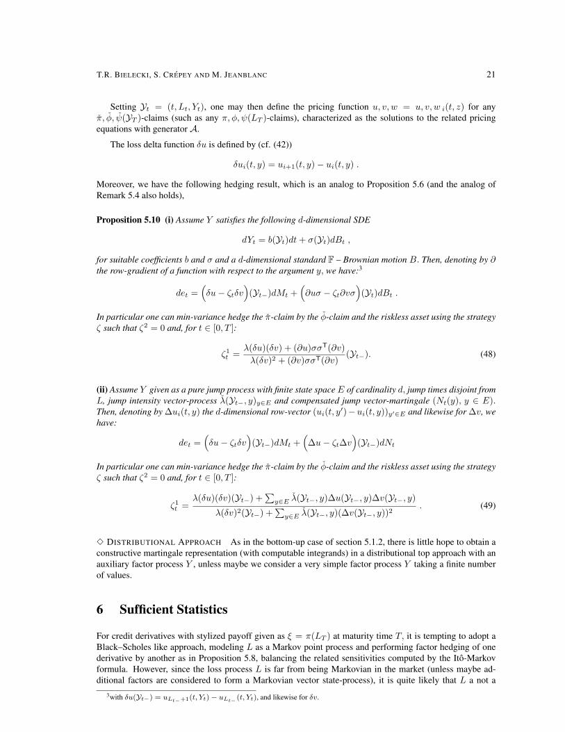
Figure 1 provides an illustration of formula (39) in a simple model with n = 3 stopping times2. Thefigure shows a trajectory over the time interval (0, 5yr) of the (pre-default) intensity of τ1 with respect toH1 ∨FZ ,H1 ∨H2 ∨FZ and H1 ∨H2 ∨H3 ∨FZ (respectively labelled lambda1, lambda2 and lambda3in the Figure), where the Hi’s correspond to the filtrations generated by the Hi’s, and:• the reference filtration FZ is trivial in the left pane,• it is given as a (scalar) Brownian filtration FZ = FW in the right pane.We refer the reader to Zargari [43] for every detail about these simulations. On this example we have τ2 =1.354, τ3 = 0.669 in the case where FZ is trivial and τ2 = 1.3305, τ3 = 0.676 in the case where FZ = FW
(the same random numbers were used in the two experiments). Observe that:• lambda2 and lambda3 jump at τ2(= 1.354 in the left pane and 1.3305 in the right pane),• only lambda3 jumps at τ3(= 0.669 in the left pane and 0.676 in the right pane), and• lambda1 does not jump at all.Also note the effect of adding a reference filtration (noisy pre-default intensities in the right-pane, versuspre-default intensities ‘deterministic between default times’ in the left pane).
As for hedging, it seems difficult to derive explicit and constructive martingale representations in theset-up of this paragraph (so hedging cannot be implemented either), unless we are in the case of an aux-iliary factor process Z given as a pure jump process with finite state space. In this case it is possible toderive an elementary martingale representation and a suitable analog to Proposition 5.6(ii), valid for payoffsπ, φ, ψ (τ1, τ2). The detail is left to the reader.
5.2 Top Approaches
We now work with a top filtration F.We directly consider n default times. Since we work with a top filtrationF, the τi’s are not F-stopping times, as opposed to the ordered default times ti’s. The loss process is therefore
2We thank Behnaz Zargari from the Mathematics Departments at University of Evry, France, and University of Sharif, Iran, for thesesimulations.

T.R. BIELECKI, S. CREPEY AND M. JEANBLANC 19
an F-adapted, non-decreasing process. We denote by M its F – compensated martingale, so
M = L−∫ ·
0
λtdt
where λ is the (predictable version of the) F-intensity, assumed to exist, of L.
5.2.1 Pure Top Approaches
Here F = FL.
3 MARKOVIAN APPROACH In the Markovian case L is a pure birth-and-death process (local intensityprocess as of Laurent, Cousin and Fermanian [36] or Cont and Minca [11]), with F-intensity λt = λ(t, Lt),for a suitable F-intensity function λ(t, i) (vanishing for i ≥ n, consistently with the fact that the loss processL is stopped at level n).
In this set-up, we obtain that, for t ∈ [0, T ]
Πt = E(π(LT ) | Ft) = u(t, Lt) , (40)
where u(t, i) or ui(t) for (t, i) ∈ [0, T ] × Nn, is the pricing function (system of time-functionals ui), solu-tion to the related system of backward Kolmogorov differential equations. Moreover we have the followingmartingale representation, for t ∈ [0, T ]:
Πt = u(t, Lt) = E(π(LT )) +∫ t
0
δu(s, Ls−) dMs (41)
where the delta function δu is defined by, for t ∈ [0, T ] and i ∈ Nn−1 :
δui(t) = ui+1(t)− ui(t) . (42)
It is rather clear that in this present case it is enough to use just one claim, say φ (and the riskless account) soto replicate claim π. So, using the analogous martingale representation for the φ claim, the following resultfollows (in view of (17)),
Proposition 5.8 One can replicate π(LT ) at T by using the strategy ζ based on the φ-claim (and on theriskless asset) defined by, for t ∈ [0, T ] (assuming δv 6= 0):
ζt =δu
δv(t, Lt−) .
3 DISTRIBUTIONAL APPROACH We denote Git(u) = P(Lu = i | Ft), for i ∈ Nn.
As an FL-martingale, the process Git(u) admits a representation of the form
Git(u) = Gi
0(u) +∫ t
0
δGis(u) dMs
for some integrand δGis(u). We are now ready to write the representation for Π in terms of δG. We thus
have, for t ∈ [0, T ] :
Πt =∑
0≤i≤n
π(i)Git(T ) = E(π(LT )) +
∫ t
0
δΠs dMs , (43)
where we setδΠt =
∑0≤i≤n π(i)δGi
t(T ) .
Using the analogous representation regarding the φ claim, and plugging all these expressions in (17), one getsthe following,
20 UP AND DOWN CREDIT RISK
Proposition 5.9 One can replicate π at T by using the strategy ζ based on the φ-claim (and on the risklessasset) defined by, for t ∈ [0, T ] (assuming δΦt 6= 0):
ζt =δΠt
δΦt. (44)
To illustrate the feasibility (and the limits) of the approach of this paragraph we need to provide specificexamples in which Gi
t(u) and δGit(u) are computable. For this it is enough that the joint cumulative dis-
tribution of the consecutive default times tk’s of L be computable and continuous. Indeed we have, sinceF = FL :
Git(u) = P(Lu = i | Ft) = P(Lu = i | Ft ∨ σ(Lt)) , (45)
which on the random time interval t ∈ [tl, tl+1) (or, equivalently, on the event Lt = l), is easily seen tocoincide with P(ti ≤ u < ti+1 | t1, · · · , tl ;, tl ≤ t < tl+1). Now, by the Bayes rule, the latter quantity isdetermined by the joint law of the tk’s. Moreover, if the cumulative distribution of (tk)1≤k≤n is continuous,then Gi
t(u) is thus continuous on every interval [tl, tl+1), and the only possible jumps of Git(u) occur at the
tl’s, where they are given by
Gitl(u)−Gi
tl−(u) = P(ti ≤ u < ti+1 | t1, · · · , tl)− P(ti ≤ u < ti+1 | t1, · · · , tl−1) , (46)
which can also be evaluated by the Bayes rule given the joint cumulative distribution of the tk’s. So δGit(u)
is computable too.
Example 5.5 We consider two ordered times t1 and t2 defined by, given IID unit exponential random vari-ables E1 and E2 :
t1 = inft > 0 |∫ t
0
µ1(s)ds > E1 , t2 = inft > t1 |∫ t
t1
µ2(s, t1)ds > E2
with µ1(t) = 1 , µ2(t, t1) = t1. So
t1 = E1 , t2 = t1 +E2
t1.
One can show that the related loss process L is a non-Markovian Hawkes process (see Errais, Giesecke andGoldberg [19], Hawkes [28]). Moreover, we have in this case
P(t1 > u1, t2 > u2) = P(u1 < E1, u2 < E1 +E2
E1) ,
which is explicitly given by∫
x>u1
∫y>x(u2−x)+
e−(x+y)dxdy . Git(u) and δGi
t(u) can thus be computed, andso can in turn be δΠ, δΦ and ζ in (44).
5.2.2 Adding a Reference Filtration
We now assume F = FL ∨ FY , for a suitable factor process Y .
3 MARKOVIAN APPROACH We suppose that the pair (L, Y ) is an F – Markov process with generator A,assuming more specifically that the F-intensity of L satisfies
λt = λ(t, Lt, Yt) (47)
for a given intensity function λi(t, y) (vanishing for i ≥ n). The construction of such a model (L, Y ) can berealized by a Markovian change of probability measure, starting from an auxiliary model with independentloss and factor processes.
T.R. BIELECKI, S. CREPEY AND M. JEANBLANC 21
Setting Yt = (t, Lt, Yt), one may then define the pricing function u, v, w = u, v, w i(t, z) for anyπ, φ, ψ(YT )-claims (such as any π, φ, ψ(LT )-claims), characterized as the solutions to the related pricingequations with generator A.
The loss delta function δu is defined by (cf. (42))
δui(t, y) = ui+1(t, y)− ui(t, y) .
Moreover, we have the following hedging result, which is an analog to Proposition 5.6 (and the analog ofRemark 5.4 also holds),
Proposition 5.10 (i) Assume Y satisfies the following d-dimensional SDE
dYt = b(Yt)dt+ σ(Yt)dBt ,
for suitable coefficients b and σ and a d-dimensional standard F – Brownian motion B. Then, denoting by ∂the row-gradient of a function with respect to the argument y, we have:3
det =(δu− ζtδv
)(Yt−)dMt +
(∂uσ − ζt∂vσ
)(Yt)dBt .
In particular one can min-variance hedge the π-claim by the φ-claim and the riskless asset using the strategyζ such that ζ2 = 0 and, for t ∈ [0, T ]:
ζ1t =
λ(δu)(δv) + (∂u)σσT(∂v)λ(δv)2 + (∂v)σσT(∂v)
(Yt−). (48)
(ii) Assume Y given as a pure jump process with finite state spaceE of cardinality d, jump times disjoint fromL, jump intensity vector-process λ(Yt−, y)y∈E and compensated jump vector-martingale (Nt(y), y ∈ E).Then, denoting by ∆ui(t, y) the d-dimensional row-vector (ui(t, y′)−ui(t, y))y′∈E and likewise for ∆v, wehave:
det =(δu− ζtδv
)(Yt−)dMt +
(∆u− ζt∆v
)(Yt−)dNt
In particular one can min-variance hedge the π-claim by the φ-claim and the riskless asset using the strategyζ such that ζ2 = 0 and, for t ∈ [0, T ]:
ζ1t =
λ(δu)(δv)(Yt−) +∑
y∈E λ(Yt−, y)∆u(Yt−, y)∆v(Yt−, y)
λ(δv)2(Yt−) +∑
y∈E λ(Yt−, y)(∆v(Yt−, y))2. (49)
3 DISTRIBUTIONAL APPROACH As in the bottom-up case of section 5.1.2, there is little hope to obtain aconstructive martingale representation (with computable integrands) in a distributional top approach with anauxiliary factor process Y , unless maybe we consider a very simple factor process Y taking a finite numberof values.
6 Sufficient Statistics
For credit derivatives with stylized payoff given as ξ = π(LT ) at maturity time T, it is tempting to adopt aBlack–Scholes like approach, modeling L as a Markov point process and performing factor hedging of onederivative by another as in Proposition 5.8, balancing the related sensitivities computed by the Ito-Markovformula. However, since the loss process L is far from being Markovian in the market (unless maybe ad-ditional factors are considered to form a Markovian vector state-process), it is quite likely that L a not a
3with δu(Yt−) = uLt−+1(t, Yt)− uLt− (t, Yt), and likewise for δv.

22 UP AND DOWN CREDIT RISK
sufficient statistics for the purpose of valuation and hedging of portfolio credit risk. In other words, ignoringthe potentially non-Markovian dynamics of L for pricing and/or hedging may cause significant model risk,even though the payoffs of the products at hand are given as functions of LT .
In this section we want to illustrate this point by means of numerical hedging simulations. For morerealism in these numerical experiments we introduce a non-zero recovery R, taken as a constant R = 40%.We thus need to distinguish the cumulative default process Nt =
∑ni=1 H
it and the cumulative loss process
Lt = (1−R)Nt.
We shall consider the benchmark problem of pricing and hedging a stylized loss derivative. Specifically,for simplicity, we only consider protection legs of of equity tranches , resp. super-senior tranches (i.e.detachment of 100%), with stylized payoffs
π(NT ) =LT
n∧ k , resp. (
LT
n− k)+
at a maturity time T . The ‘strike’ (detachment, resp. attachment point) k belongs to [0, 1]. In this formalismthe (stylized) credit index corresponds to the equity tranche with k = 100% (or senior tranche with k = 0).With a slight abuse of terminology, we shall refer to our stylized loss derivatives as to tranches and index,respectively.
We shall now consider the problem of hedging the tranches with the index, using a simplified marketmodel of credit risk.
6.1 Homogeneous Groups Model
We consider a Markov chain model of credit risk as of Frey and Backhaus [21] (see also Bielecki et al. [3]).Namely, the n names of a pool are grouped in d classes of ν − 1 = n
d homogeneous obligors (assuming nd
integer), and the cumulative default processes N l, l ∈ N∗d, of the different groups (so N =
∑N l) are jointly
modeled as a d-variate Markov point process N , with FN -intensity of N l given as
λlt = (ν − 1−N l
t)λl(t,Nt) , (50)
for some pre-default individual intensity functions λl = λl(t, ı), where ı = (i1, · · · , id) ∈ Ndν−1. The related
generator (spatial generator at time t) may then be written in the form of a νd-dimensional (very sparse)matrix At.
For d = 1, we recover the well-known local intensity model already considered in the first paragraph ofSection 5.2.1 (pure top approach with N modeled as a Markov birth point process stopped at level n; see, forinstance, Laurent, Cousin and Fermanian [36] or Cont and Minca [11]. At the other extreme, for d = n, weare in effect modeling the vector of the default indicator processes of the pool names. As d varies between1 and n, we thus get a variety of models of credit risk, ranging from pure top models for d = 1 to purebottom-up models for d = n.
Remark 6.1 Observe that in the homogeneous case where λl(t, ı) = λ(t,∑
j ij) for some function λ =λ(t, i) (independent of l), the model (whatever the nominal value of d / structure of the matrix generator usedfor encoding the model) effectively reduces to a local intensity model (with d = 1 and pre-default individualintensity λ(t, i) therein).Further specifying the model to λ independent of i corresponds to the situation of homogeneous and inde-pendent obligors.In general, introducing parsimonious parameterizations of the intensities allows one to account for inhomo-geneity between groups and/or defaults contagion. It is also possible to extend this set-up to more generalcredit migrations models, or to generic bottom-up models of credit migrations influenced by macro-economicfactors (see Bielecki et al. [3, 8] or Frey and Backhaus [22]).
Note that we only use this model for its flexibility and ease of implementation in view of illustrativepurposes. We are not claiming here that this would be a good model for dealing with credit derivatives inactual practice (cf. in particular the reservation made in Section 3.2.1).
T.R. BIELECKI, S. CREPEY AND M. JEANBLANC 23
6.1.1 Pricing in the Homogeneous Groups Model
Since N is a Markov process andN is a function of N , the related tranche price process writes, for t ∈ [0, T ](assuming π(NT ) integrable):
Πt = E(π(NT ) | FNt ) = u(t,Nt) , (51)
where u(t, ı) or uı(t) for t ∈ [0, T ] and ı ∈ Ndν−1, is the pricing function (system of time-functions uı).
Using the Ito formula in conjunction with the martingale property of Π, the pricing function can then becharacterized as the solution to the following pricing equation (system of ODEs):
(∂t +At)u = 0 on [0, T ) (52)
with terminal condition uı(T ) = π(ı), for ı ∈ Ndν−1. In particular, in the case of a time-homogeneous
generator A (independent of t), one has the semi-closed formula,
u(t) = exp[(T − t)A]π . (53)
Pricing in this model can be achieved by various means, like numerical resolution of the ODE system (52),numerical matrix exponentiation based on (53) (in the time-homogeneous case) or Monte Carlo simulation.However resolution of (52) or computation of (53) by deterministic numerical schemes is typically precludedby the curse of dimensionality for d greater than a few units (depending on ν). So for high d simulationmethods appear to be the only viable computational alternative. Appropriate variance reduction methodsmay help in this regard (see, for instance, Carmona and Crepey [12]).
The distribution of the vector of time-t losses (for each group), that is, qı(t) = P(Nt = ı) for t ∈ [0, T ]and ı ∈ Nd
ν−1, and the portfolio cumulative loss distribution, p = pi(t) = P(Nt = i) for t ∈ [0, T ] andi ∈ Nn, can be computed likewise by numerical solution of the associated forward Kolmogorov equations(for more detail, see, e.g., [12]).
6.1.2 Hedging in the Homogeneous Groups Model
In general, in the Markovian model described above, it is possible to replicate dynamically in continuoustime any payoff provided d non-redundant hedging instruments are available (see Frey and Backhaus [20]or Bielecki, Vidozzi and Vidozzi [8]; see also Laurent, Cousin and Fermanian [36] for results in the specialcase where d = 1). From the mathematical side this corresponds to the fact that the model is of multiplicityd (see, e.g., Davis and Varaiya[14]), in general. So, in general, it is not possible to replicate a payoff, such astranche, by the index alone in this model, unless the model dimension d is equal to one (or reducible to one,cf. Remark 6.1). Now our point is that this potential lack of replicability is not purely speculative, but can bevery significant in practice.
Since delta-hedging in continuous time is expensive in terms of transaction costs, and because mainchanges occur at default times in this model (in fact, default times are the only events in this model, if not fortime flow and the induced time-decay effects), we shall focus on semi-static hedging in what follows, onlyupdating at default times the composition of the hedging portfolio. More specifically, denoting by t1 the firstdefault time of a reference obligor, we shall examine the result at t1 of a static hedging strategy on the randomtime interval [0, t1].Let Π and P denote the tranche and index model price processes, respectively. Using a constant hedge ratioδ0 over the time interval [0, t1], the tracking error or profit-and-loss of a delta-hedged tranche at t1 writes:
et1 = (Πt1 −Π0)− δ0(Pt1 − P0) . (54)
The question we want to consider is whether it is possible to make this quantity ‘small’, in terms, say, of(risk-neutral) variance, relative to the variance of Πt1 −Π0 (which corresponds to the risk without hedging),by a suitable choice of δ0. It is expected that this should depend:• First, on the characteristics of the tranche, and in particular on the value of the strike k: A high strike equity
24 UP AND DOWN CREDIT RISK
tranche or low strike senior tranche (in-the-money tranche) is quite close to the index in terms of cashflows,and should therefore exhibit a higher degree of correlation and be easier to hedge with the index, than a lowstrike equity tranche or high strike senior tranche (out-of-the money tranche);• Second, on the ‘degree of Markovianity’ of the loss process L, which in the case of the homogeneousgroups model depends both on the model nominal dimension d and on the specification of the intensities(see, e.g., Remark 6.1).
Moreover, it is intuitively clear that for too large values of t1 time-decay effects matter and the hedgeshould be rebalanced at some intermediate points of the time interval [0, t1] (even though no default occurredyet). To keep it as simple as possible we shall merely apply a cutoff and restrict our attention to the randomset ω : t1(ω) < T1 for some fixed T1 ∈ [0, T ].
6.2 Numerical Results
We work with the above model for d = 2 and ν = 5. We thus consider a two-dimensional model of a stylizedcredit portfolio of n = 8 obligors. The model generator is a νd ⊗ νd – (sparse) matrix with ν2d = 54 = 625.Recall that the computation time for exact pricing (using matrix exponentiation based on (53)) in such modelgrows as ν2d, which motivated the previous modest choices for d and ν.
Moreover we take the λl’s given by, (cf. (50)):
λ1(t, ı) =2(1 + il)
9n, λ2(t, ı) =
16(1 + il)9n
. (55)
So in this case (which is an admittedly extreme case of inhomogeneity between two independent groups ofobligors), the individual intensities of the obligors of group 1 and 2 are given as 1+i1
36 and 8(1+i2)36 , where i1
and i2 represent the number of currently defaulted obligors in groups 1 and 2, respectively.For instance, at time 0 with N0 = (0, 0), the individual intensities of obligors of group 1 and 2 are equal to1/36 and 8/36, respectively; the average individual intensity at time 0 is thus equal to 1/8 = 0.125 = 1/n.
We set the maturity T equal to 5 years and the cutoff T1 equal to 1 year. We thus make a focus on therandom set of trajectories for which t1 < 1, meaning that a default occurred during the first year of hedging.
6.2.1 Model Simulation
In this toy model the simulation takes the following very simple form (see also [20] or [3] for more details inmore general set-ups):Compute Π0 (for the tranche) and P0 (for the index) by numerical matrix exponentiation based on (53), andthen for every j = 1, · · · ,m:• Draw a pair (tj1, t
j1) of independent exponential random variables with parameter (cf. (50)–(55))
(λ10, λ
20) = 4× (
136,
836
) = (19,89) ; (56)
• Set tj1 = min(tj1, tj1) and Nt1 = (1, 0) or (0, 1) depending on whether tj1 = tj1 or tj1;
• Compute Πtj1
(for the tranche) and Ptj1
(for the index) by (53).
Doing this for m = 104, we got 9930 draws with t1 < T = 5yr, among which 6299 ones with t1 <T1 = 1yr, subdividing themselves into 699 defaults in the first group of obligors and 5600 defaults in thesecond one.
6.2.2 Pricing Results
We consider two T = 5yr-tranches in the above model: an ‘equity tranche’ with k = 30%, corresponding toa payoff (1−R)NT
n ∧ k = (60NT
8 ∧ 30)% (of a unit nominal amount), and a ‘senior tranche’ defined simply asthe complement of the equity tranche to the index, thus with payoff ( (1−R)NT
n − k)+ = (60NT
8 − 30)+%.

T.R. BIELECKI, S. CREPEY AND M. JEANBLANC 25
We also computed the portfolio loss distribution at maturity by numerical matrix exponentiation corre-sponding to explicit solution of the associated forward Kolmogorov equations (see, e.g., [12]).
Note that there is virtually no error involved in the previous computations, in the sense that our simulationis exact (without simulation bias), and the prices and loss probabilities are computed by (quasi-exact) matrixexponentiation.
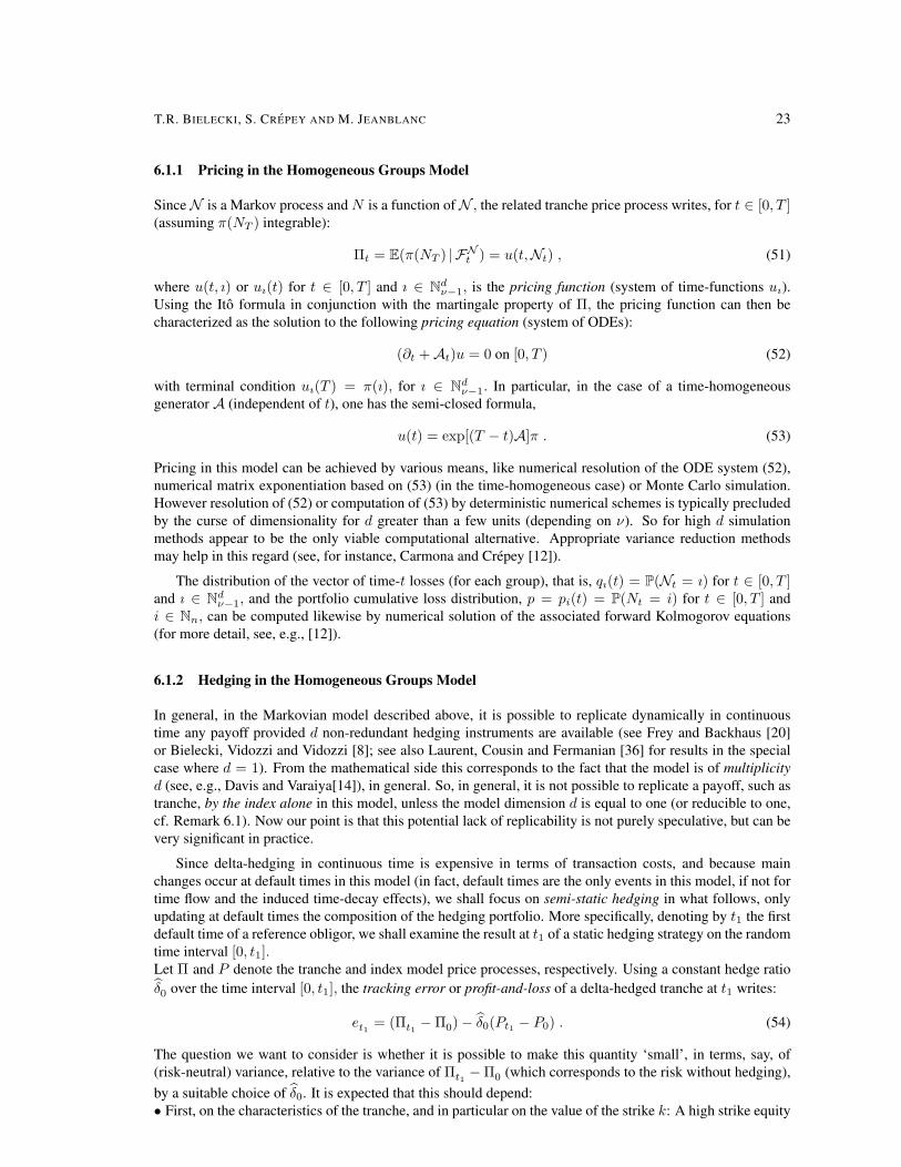
The left pane of Figure 2 represents the histogram of the loss distribution at the time horizon T ; weindicate by a vertical line the loss level x beyond which the equity tranche is wiped out, and the seniortranche starts being hit (so (1−R)x
n = k, e.g. x = 4).The right pane of Figure 2 displays the equity (labeled by +), senior (×) and index () tranche prices at t1(in ordinate) versus t1 (in abscissa), for all the points in the simulated data with t1 < 5 (9930 points). Blueand red points correspond to defaults in the first (Nt1 = (1, 0)) and in the second (Nt1 = (0, 1)) group ofobligors, respectively. We also represented in black the points (0,Π0) (for the tranches) and (0, P0) (for theindex).
Note that in the case of the senior tranche and of the index, there is a clear difference between prices at t1depending on whether t1 corresponds to a default in the first or in the second group of obligors, whereas inthe case of the equity tranche there seems to be little difference in this regard.In view of the portfolio loss distribution in the left pane, this can be explained by the fact that in the case ofthe equity tranche, the probability conditional on t1 that the tranche will be wiped out at maturity is importantunless t1 is rather large. Therefore the equity tranche price at t1 is close to k = 30% for t1 close to 0.Moreover for t1 close to T the intrinsic value of the tranche at t1 constitutes the major part of the equitytranche price at t1 (since the tranche has low time-value close to maturity). In conclusion the state of N at t1has a low impact on Πt1 , unless t1 is in the middle of the time-domain.On the other hand, in the case of the senior tranche or in case of the index, the state of N at t1 has a highimpact on the corresponding price, unless t1 is close to T (in which case intrinsic value effects are dominant).This explains the ‘two-track’ pictures seen for the senior tranche and for the index on the right pane of Figure2, except close to T (whereas the two-tracks are superimposed close to 0 and T in the case of the equitytranche).
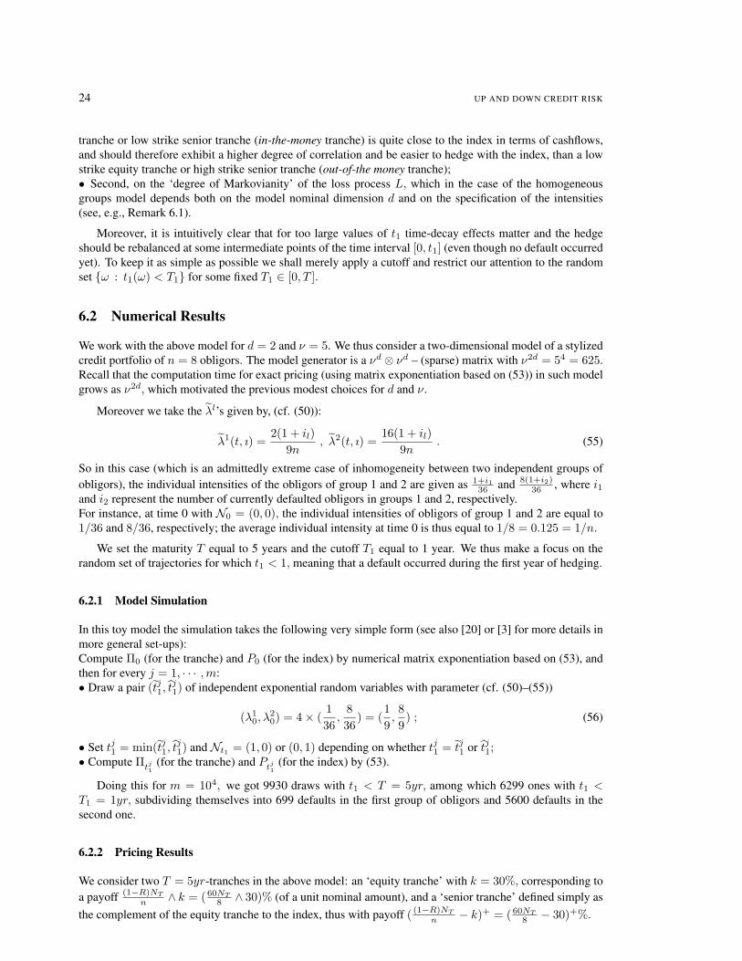
Looking at these results in terms of price changes Π0 − Πt1 of a tranche versus the corresponding indexprice changes P0 − Pt1 , we obtain the graphs of Figure 3 for the equity tranche and 4 for the senior tranche.We consider all points with t1 < T on the left panes and focus on the points with t1 < T1 on the right ones.We use the same blue/red color code as above, and we further highlight in green on the left panes the pointswith t1 < 1, which are focused upon on the right panes.Figure 3 gives a further graphical illustration of the low level of correlation between price changes of theequity tranche and of the index. Indeed the cloud of points on the right pane is obviously “far from a straightline”, due to the partitioning of points between blue points / defaults in group one on one segment versus redpoints / defaults in group two on a different segment.On the opposite (Figure 4), at least for t1 not too far from 0 (right pane), there is an evidence of linearcorrelation between price changes of the senior tranche and of the index, since in this case the blue and thered segments are not far from being on a common line.
6.2.3 Hedging Results
We then computed the (empirical, risk-neutral) variance of Πt1 − Π0 and of the profit-and-loss et1 in (54)(restricting attention to the subset t1 < T1 = 1), using for δ0 the empirical regression delta of the tranchewith respect to the index at time 0, so
δ0 =Cov(Πt1 −Π0, Pt1 − P0)
Var(Pt1 − P0). (57)
Moreover, we also did these computations restricting further attention to the subsets of t1 < 1 correspondingto defaults in the first and in the second group of obligors (blue and red points on the figures), respectively. The
26 UP AND DOWN CREDIT RISK
Figure 2: (Left) Portfolio loss distribution at maturity T = 5yr; (Right) Tranche Prices at t1 for t1 < T = 5(equity tranche (+), senior tranche (×) and index ()).). On this and the following figures, blue and redpoints correspond to defaults in the first and in the second group of obligors, respectively.
Figure 3: Equity tranche vs Index Price Changes between 0 and t1 (t1 < T = 5, left pane; zoom ont1 < T1 = 1, right pane).
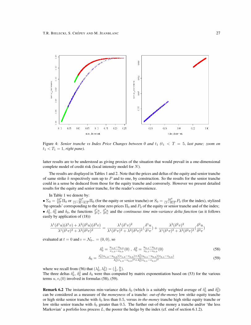
T.R. BIELECKI, S. CREPEY AND M. JEANBLANC 27
Figure 4: Senior tranche vs Index Price Changes between 0 and t1 (t1 < T = 5, last pane; zoom ont1 < T1 = 1, right pane).
latter results are to be understood as giving proxies of the situation that would prevail in a one-dimensionalcomplete model of credit risk (local intensity model for N ).
The results are displayed in Tables 1 and 2. Note that the prices and deltas of the equity and senior trancheof same strike k respectively sum up to P and to one, by construction. So the results for the senior tranchecould in a sense be deduced from those for the equity tranche and conversely. However we present detailedresults for the equity and senior tranche, for the reader’s convenience.
In Table 1 we denote by:• Σ0 = 104
kT Π0 or 104
(1−R−k)T Π0 (for the equity or senior tranche) or S0 = 104
(1−R)T P0 (for the index), stylized‘bp spreads’ corresponding to the time zero prices Π0 and P0 of the equity or senior tranche and of the index;• δ10 , δ20 and δ0, the functions δ1u
δ1v , δ2uδ2v and the continuous time min-variance delta function (as it follows
easily by application of (18))
λ1(δ1u)(δ1v) + λ2(δ2u)(δ2v)λ1(δ1v)2 + λ2(δ2v)2
=λ1(δ1v)2
λ1(δ1v)2 + λ2(δ2v)2(δ1u
δ1v) +
λ2(δ2v)2
λ1(δ1v)2 + λ2(δ2v)2(δ2u
δ2v)
evaluated at t = 0 and ı = N0− = (0, 0), so
δ10 = u1,0−u0,0v1,0−v0,0
(0) , δ20 = u0,1−u0,0v0,1−v0,0
(0) (58)
δ0 = λ10(u1,0−u0,0)(v1,0−v0,0)+λ2
0(u0,1−u0,0)(v0,1−v0,0)
λ10(v1,0−v0,0)
2+λ20(v0,1−v0,0)
2 (59)
where we recall from (56) that (λ10, λ
20) = ( 1
9 ,89 ).
The three deltas δ10 , δ20 and δ0 were thus computed by matrix exponentiation based on (53) for the various
terms u, vı(0) involved in formulas (58), (59).
Remark 6.2 The instantaneous min-variance delta δ0 (which is a suitably weighted average of δ10 and δ20)can be considered as a measure of the moneyness of a tranche: out-of-the-money low strike equity trancheor high strike senior tranche with δ0 less than 0.5, versus in-the-money tranche high strike equity tranche orlow strike senior tranche with δ0 greater than 0.5. The further out-of-the money a tranche and/or ‘the lessMarkovian’ a porfolio loss process L, the poorer the hedge by the index (cf. end of section 6.1.2).

28 UP AND DOWN CREDIT RISK
Π0 or P0 Σ0 or S0 δ10 δ20 δ0Eq 0.2821814 1881.209 0.1396623 0.7157741 0.2951399Sen 0.03817907 254.5271 0.8603377 0.2842259 0.7048601
Table 1: Time t = 0 – Prices, Spreads and Instantaneous Deltas in the Semi-Homogeneous Model.
In Table 2 (cf. also (57)):• ρ in column two is the empirical correlation of the tranche price increments Πt1−Π0 versus the index priceincrements Pt1 − P0,• R2 = ρ2 in column three is the coefficient of determination of the regression,• Dev in column 4 stands for Stdev(Πt1 −Π0)/Π0,
• The hedging variance reduction factor RedVar = Var(Πt1−Π0)
Var(et1 )in the last column is equal to 1
1−ρ2 .
Remark 6.3 It is expected that δ0 should converge to δ0 in the limit where the cutoff T1 would tend to zero,provided the number of simulations m jointly goes to infinity. For T1 = 1yr and m = 104 simulationshowever, we shall see below that there is a clear discrepancy between δ0 and δ0, and all the more so that weare in a non-homogeneous model with low correlation between the tranche and index price changes betweentimes 0 and t1. The reason is that the coefficient of determination (R2) of the linear regression with slope δ0is given by R2 = ρ2. In case ρ is small, R2 is even smaller, and the significance of the estimator (for lowT1’s) δ0 of δ0 is low too. In other words, in case ρ is small, we recover mainly noise through δ0; this howeverdoes not weaken our statements below regarding the ability or not to hedge the tranche by the index, since
the variance reduction factor RedVar = Var(Πt1−Π0)
Var(et1 )is equal to 1
1−ρ2 , which only depends on ρ and not on
δ0.
δ0 ρ R2 Dev RedVarEq -0.00275974 -0.03099014 0.0009603885 0.006612626 1.000961
Eq1 0.2269367 0.9980242 0.9960522 0.007576104 253.306Eq2 0.3391563 0.997375 0.994757 0.006134385 190.7276Sen 1.002760 0.9960836 0.9921825 0.07475331 127.9176
Sen1 0.7730633 0.9998293 0.9996586 0.02576152 2928.847Sen2 0.6608437 0.9993066 0.9986137 0.01192970 721.3244
Table 2: Hedging Tranches by the Index in the Semi-Homogeneous Model.
Recall that qualitatively the senior tranche’s dynamics is rather close to that of the index (at least for t1close to 0, see Section 6.2.2, right pane of Figure 4). Accordingly, we find that hedging the senior tranchewith the index is possible (variance reduction factor of about 128 in bold blue in the last column). Thiscase thus seems to be supportive of the claim according to which one could use the index for hedging a lossderivative, even in a non Markovian model of portfolio loss process L.
But in the case of the equity tranche we get the opposite message: the index is useless for hedgingthe equity tranche (variance reduction factor essentially equal to 1 in bold red in the table, so no variancereduction in this case).Moreover, the equity tranche variance reduction factors conditional on defaults in the first and in the secondgroup of obligors (in purple in the table) amount to 253 and 190, respectively. This supports the interpretationthat the unhedgeability of the equity tranche by the index really comes from the fact that the full modeldynamics is not represented in the loss process.
Incidentally this also means that hedging the senior tranche by the equity tranche, or vice versa, is notpossible either.

T.R. BIELECKI, S. CREPEY AND M. JEANBLANC 29
We conclude that in general, at least for certain ranges of the model parameters and tranche characteristics(strong to strong non-Markovianity of L and out-of-the money to far out-of-the money tranche), hedgingtranches with the index may not be possible in a non Markovian model of portfolio loss process L.
Since the equity and the senior tranche sum-up to the index, therefore a perfect static replication of theequity tranche (say) is provided by a long position in the index and a short position in the senior tranche. Asa reality-check of this statement, we performed a bilinear regression of the equity price increments versusthe index and the senior tranche price increments, in order to minimize over (δind
0 , δsen0 ) the (risk-neutral)
variance of
et1 = (Πeqt1 −Πeq
0 )− δind0 (Pt1 − P0)− δsen
0 (Πsent1 −Πsen
0 ) . (60)
The results are displayed in Tables 3. We recover numerically the perfect two-instruments replication strategymentioned above, whereas a single-instrument hedge using only the index was essentially useless in this case(cf. bold red entry in Table 2).
δind0 δsen
0 RedVar1 -1 2.566254e+29
Table 3: Replicating the equity tranche by the index and the senior tranche in the Semi-Homogeneous Model.
6.2.4 Fully Homogeneous Case
For confirmation of the previous analysis and interpretation of the results, we redid the computations usingthe same values as before for all the model, products and simulation parameters, except for the fact that thefollowing pre-default individual intensities were used, for l = 1, 2 :
λl(ı) =1n
+
∑1≤`≤d i`
nd=: λ(
∑1≤`≤d
i`) . (61)
For instance, at time 0 with N0 = 0, the individual intensities of the obligors are all equal to 1/8 = 0.125 =1/n.
We are thus in a case of homogeneous obligors, reducible to a local intensity model (with d = 1 andpre-default individual intensity λ(i) therein, see Remark 6.1). So in this case we expect that hedging tranchesby the index should work, including in the case of the out-of-the-money equity tranche.
This is what happens numerically, as it is evident from the following Figures and Tables (which are theanalogs of those in previous sections, using the same notation everywhere). Note that all red and blue curvesare superimposed, which is consistent with the fact that the group of a defaulted name has no bearing in thiscase, given the present specification of the identities.
Out of new 104 draws using the intensities given in (61), we got 9922 draws with t1 < 5, among which6267 ones with t1 < 1, subdividing themselves into 3186 defaults in the first group of obligors and 3081defaults in the second one.
Looking at Table 5, we find as in the semi-homogeneous case that hedging the senior tranche with theindex works very well (still better than before, variance reduction factor of 11645 in bold blue in the lastcolumn; yet this may be partly due to a moneyness effect: the senior tranche is further in-the-money thanbefore, with an senior tranche δ0 of about 0.7 in Table 1 versus 0.8 in Table 4).But as opposed to the situation in the semi-homogeneous case, hedging the equity tranche with the index alsoworks very well (variance reduction factor of about 123 in bold purple in the last column), and this holdseven though the equity tranche is further out-of-the-money now than it was before, with an equity tranche δ0of about 0.3 in Table 1 versus 0.2 in Table 4 (cf. Remark 6.2). So the degradation of the hedge when we passfrom the homogeneous model to the semi-homogeneous model is really due to the non-Markovianity of L,
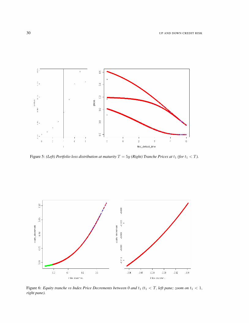
30 UP AND DOWN CREDIT RISK
Figure 5: (Left) Portfolio loss distribution at maturity T = 5y (Right) Tranche Prices at t1 (for t1 < T ).
Figure 6: Equity tranche vs Index Price Decrements between 0 and t1 (t1 < T, left pane; zoom on t1 < 1,right pane).

T.R. BIELECKI, S. CREPEY AND M. JEANBLANC 31
Figure 7: Senior tranche vs Index Price Decrements between 0 and t1 (t1 < T, left pane; zoom on t1 < 1,right pane).
and not to an effect of moneyness (cf. end of section 6.1.2).Moreover the unconditional variance reduction factor and variance reduction factor conditional on defaultsin the first and in the second group of obligors are now essentially the same (for the equity tranche as for thesenior tranche).
This also means that hedging the equity tranche by the senior tranche, or vice versa, is quite effective inthis case.
These results support our previous analysis that the impossibility of hedging the equity tranche by theindex in the semi-hompogeneous model was due to the non-Markovianity of the loss process L.
Note incidentally that δ0 and δ0 are closer now (in Tables 4–5) than they were previously (in Tables 1–2).This is consistent with the fact that R2 is now larger than before (δ0 and δ0 would be even closer if the cutoffT1 was less than 1yr, provided of course the number of simulations m is large enough; see Remark 6.3).
Π0 or P0 Σ0 or S0 δ10 δ20 δ0Eq 0.2850154 1900.103 0.2011043 0.2011043 0.2011043Sen 0.1587075 1058.050 0.7988957 0.7988957 0.7988957
Table 4: Time t = 0 – Prices, Spreads and Instantaneous Deltas in the Fully-Homogeneous Model.
δ0 ρ R2 Dev RedVarEq 0.0929529 0.9959361 0.9918887 0.004754811 123.2852Eq1 0.09307564 0.995929 0.9918745 0.004794916 123.0695Eq2 0.09282067 0.995946 0.9919084 0.004713333 123.5853Sen 0.9070471 0.999957 0.9999141 0.04621152 11645.15
Sen1 0.9069244 0.9999569 0.9999137 0.04653322 11590.83Sen2 0.9071793 0.9999573 0.9999146 0.0458808 11710.42
Table 5: Hedging Tranches by the Index in the Fully-Homogeneous Model.

32 UP AND DOWN CREDIT RISK
7 Conclusions
In case of a non (FL-)Markovian portfolio process L, factor hedging of a loss derivative by another one maynot work, and hedging by individuals is necessary.
Bottom-up models are the only ones suited for this purpose (possibly constructed top-down by thinning,admittedly).
This effectively means that the prices of credit derivatives depend on factors others than L, like theidentity (and not only the number) of the defaulted names, ratings or implied ratings (and not only identities)of survivors, etc. This makes of course perfect sense since it is rather clear that the default of a major namein the index does not bear the same informational content as that of an arbitrary firm, and, moreover, pricingis done by agents with regard to the quality of the remaining names in the portfolio rather than with regard tothe defaulted names.
At this point one may raise the issue of the so called curse of dimensionality that is commonly associatedwith the bottom-up approaches. However, recent developments in the bottom up modeling enable one toefficiently cope with this curse of dimensionality. It is thus possible to specify high-dimensional (‘bottom-up’) dynamic Markovian models of portfolio credit risk with automatically calibrated model marginals (tothe individual CDS curves, say), see Bielecki, Vidozzi and Vidozzi [8].Much like in the standard static copula framework, this effectively reduces the main computational cost issue,that relative to model calibration, to calibration of the few dependence parameters in the model at hand. Thiscalibration can thus be achieved in a very reasonable time, including by pure simulation procedures if need be(without using any closed pricing formulae, if there aren’t any in the model under consideration). Appropriatevariance reduction methods (see, e.g., [12]) may help in this regard.
A A glimpse of General Theory
In this Appendix we recall definitions and (essentially well known) results from the theory of processes usedin this paper (see, e.g., Dellacherie and Meyer [15]).
A.1 Optional Projections
Let X be an integrable process (not necessarily adapted). Then there exists a unique adapted process(oXt)t≥0, called the optional projection of X , such that, for any stopping time τ,
E(Xτ1τ<+∞ | Fτ
)= oXτ1τ<+∞ .
In case X is non-decreasing, then oX a submartingale.
A.2 Dual Predictable Projections and Compensators
Let K be a non-decreasing and bounded process (not necessarily adapted; typically in the context of thispaper, K corresponds to marginal or portfolio loss processesHi or L). Then there exists a unique predictablenon-decreasing process (Kp
t )t≥0, called the dual predictable projection of K, such that, for any positivepredictable process H:
E(∫ ∞
0
HsdKs
)= E
(∫ ∞
0
HsdKps
).
In case K is adapted, it is a sub-martingale, and it admits as such a unique Doob-Meyer decomposition
Kt = Mt + Λt (62)

T.R. BIELECKI, S. CREPEY AND M. JEANBLANC 33
where M is a uniformly integrable martingale (since K is bounded) and the compensator Λ of K is a pre-dictable finite variation process. So Kp = Λ , by identification in the Doob-Meyer decomposition.If, moreover, K is stopped at some stopping time τ, and if Kp = Λ is continuous, then Kp = Λ is alsostopped at τ , by uniqueness of the Doob-Meyer decomposition ofK = K·∧τ . In case Λ is time-differentiable,so Λ =
∫ ·0λtdt for some intensity process λ of K (also called intensity of τ, when K = 1τ≥t for some stop-
ping time τ ), the intensity process λ vanishes after τ.
Remark A.1 If K is a point-process (like a marginal or cumulative default process Hi or L in this paper),the continuity of Λ is equivalent to the ordered jump times of K being totally inaccessible stopping times(see, e.g., Dellacherie and Meyer [15]).
Moreover (see Dellacherie and Meyer [15] or Last and Brandt [35], Bremaud [9]), these definitions andresults admit straightforward extensions to integer-valued random measures (rather than non-decreasing pro-cesses) K, viewing a random measure K as a family, parameterized by κ, of non-decreasing processesKt(ω, κ), counting the jumps with mark κ in the mark space K of an underlying marked point process.
A.3 Proof of Proposition 2.1
Let Λ denote the F-predictable non-decreasing component of the F-submartingale oΛ (see section A.1). Thetower property of iterated conditional expectations yields,
E(∫ T
t
dKu − dΛu | Ft
)= E
(∫ T
t
dKu − d(oΛ)u | Ft
)= E
(∫ T
t
dKu − dΛu | Ft
)= E
(E(∫ T
t
dKu − dΛu | Ft
)| Ft
)= 0 ,
since K − Λ is an F-martingale. This proves that
Λ = Λ . (63)
Moreover, one has Λ = Λp, (see, e.g., Proposition 3 of Bremaud and Yor [7]), hence (4) follows.
Now, in case Λ and Λ are time-differentiable with related intensity processes λ and λ, (63) means that∫ t
0
λsds− E(∫ t
0
λsds | Ft) (64)
is an F-martingale. Moreover it is immediate to check, using the tower property of iterated conditionalexpectations, that
E(∫ t
0
λsds | Ft)−∫ t
0
E(λs | Fs
)ds (65)
is an F-martingale as well. By addition between (64) and (65),∫ t
0
λsds−∫ t
0
E(λs | Fs)ds
is in turn an F-martingale. Since it is also a predictable (as continuous) finite variation process, it is thus infact identically equal to 0, so for t ≥ 0,
λt = E(λt | Ft) ,
which proves (5).

34 UP AND DOWN CREDIT RISK
References
[1] ARNSDORF, M. AND HALPERIN, I. BSLP: Markovian Bivariate Spread-Loss Model for PortfolioCredit. Working Paper, 2007.
[2] BENNANI, N.: The Forward Loss Model: A Dynamic Term Structure Pricing of Portfolio CreditDerivatives. Working Paper, 2006.
[3] BIELECKI, T.R., CREPEY, S., JEANBLANC, M. AND RUTKOWSKI, M.: Valuation of basket creditderivatives in the credit migrations environment. Handbook of Financial Engineering, J. Birge and V.Linetsky eds., Elsevier, 2007.
[4] BIELECKI, T.R., CREPEY, S., JEANBLANC, M. AND RUTKOWSKI, M.: Defaultable options in aMarkovian intensity model of credit risk. Mathematical Finance, vol. 18, pp. 493-518, 2008 (updatedversion available online at www.defaultrisk.com).
[5] BIELECKI, T.R., JEANBLANC, M. AND RUTKOWSKI, M.: Hedging of Defaultable Claims, in Paris-Princeton Lectures on Mathematical Finance 2003, eds. R.A. Carmona, E. Cinlar, I. Ekeland, E. Jouini,J.A. Scheinkman, N. Touzi, Springer 2004.
[6] BIELECKI, T.R. AND RUTKOWSKI, M.: Credit Risk: Modeling, Valuation and Hedging. Springer-Verlag, Berlin, 2002.
[7] BREMAUD, P. AND YOR, M.: Changes of filtrations and of probability measures. Z. Wahrschein-lichkeitstheorie verw. Gebiete, 45, 269–295, 1978.
[8] BIELECKI, T.R., VIDOZZI, A. AND VIDOZZI, L.: A Markov Copulae Approach to Pricing andHedging of Credit Index Derivatives and Ratings Triggered Step–Up Bonds, J. of Credit Risk, 2008.
[9] BREMAUD, P.: Point processes and queues, martingale dynamics, Springer, 1981.
[10] COCULESCU, D. NIKEGHBALI, A.: Hazard Process and Martingale Hazard Process, Working Paper,2008.
[11] CONT, R., MINCA, A.: Recovering Portfolio Default Intensities Implied by CDO Quotes, WorkingPaper, 2008.
[12] CREPEY, S. AND CARMONA, R. : Importance Sampling and Interacting Particle Systems for theEstimation of Markovian Credit Portfolios Loss Distribution, Submitted, 2008.
[13] DAI PRA, P., RUNGGALDIER, W., SARTORI, E., TOLOTTI, M.: Large portfolio losses; A dynamiccontagion model. Working Paper, 2007.
[14] DAVIS, M.H. AND VARAIYA, P.: The multiplicity of an increasing family of σ-fields, Annals ofProbab., 2(1974), 958–963.
[15] DELLACHERIE, C. AND MEYER, P.-A.: Probabilities and Potential, North-Holland, 1982.
[16] DUFFIE, D. AND GARLEANU: Risk and valuation of collateralized debt olbligations. Financial Ana-lysts Journal, 7 (1), 4159, 2001.
[17] EHLERS, P., SCHONBUCHER, P.: Background Filtrations and Canonical Loss Processes for Top-Down Models of Portfolio Credit Risk. Working Paper, 2006.
[18] EL KAROUI, N., JEANBLANC, M. AND JIAO, Y.: Modelling of Successive Defaults Events withdensity. Working Paper.
[19] ERRAIS, E., GIESECKE, K., GOLDBERG, L.: Pricing Credit from the Top Down with Affine PointProcesses. Working Paper, 2007.
[20] FREY, R., BACKHAUS, J.: Dynamic Hedging of Synthetic CDO Tranches with Spread Risk andDefault Contagion. Working Paper, 2007.

T.R. BIELECKI, S. CREPEY AND M. JEANBLANC 35
[21] FREY, R., BACKHAUS, J.: Pricing and Hedging of Portfolio Credit Derivatives with Interacting De-fault Intensities. Working Paper, 2007.
[22] FREY, R., BACKHAUS, J.: Portfolio credit risk models with interacting default intensities: a Marko-vian approach. Working Paper, 2004.
[23] GASPAR, R., SCHMIDT, T.,: Quadratic Models for Portfolio Credit Risk with Shot-Noise Effects.Working Paper, 2008.
[24] GIESECKE, K., GOLDBERG, L.: A Top Down Approach to Multi-Name Credit. Working Paper, 2007.
[25] GIESECKE, K., WEBER, S.: Credit Contagion and Aggregate Losses. Journal of Economic Dynamicsand Control, 30, Issue 5, pp. 741-767, 2006 .
[26] HALPERIN, I.: The “Top” and the “Down” in Credit Top Down Models. Slides of Presentation atCredit Risk Summit, New York, November 2, 2007.
[27] HALPERIN, I. AND TOMECEK, P.: Climbing Down from the Top: Single Name Dynamics in CreditTop Down Models. Working paper, Quantitative Research JP Morgan, September 2008.
[28] HAWKES, A.: Spectra of some self-exciting and mutually exciting point processes. Biometrika, 58(1971), pp. 8390.
[29] HERBERTSSON, A.: Pricing kth-to-default swaps under default contagion: the matrix-analytic ap-proach. The Journal of Computational Finance, (1-30) Volume 12/Number 1, Fall 2008.
[30] HERBERTSSON, A.: Pricing portfolio credit derivatives. PhD Thesis, Goteborg University, 2007.
[31] INGLIS, S., LIPTON, A., SAVESCU, I., SEPP, A.: Dynamic credit models Statistics and Its Interface,Forthcoming.
[32] JACOD, J.: Calcul Stochastique et Problemes de Martingales. Lecture Notes in Mathematics, vol. 714,Srpinger-Verlag, 1979.
[33] JEANBLANC, M. AND LE CAM, Y.: Progressive enlargement of filtrations with initial times. Workingpaper.
[34] JIAO, Y.: Le risque de credit: modelisation et simulation numerique. PhD Thesis (in English), Ecolepolytechnique.
[35] LAST, G., BRANDT, A.: Marked Point Processes on the Real Line: The Dynamical Approach,Springer, 1995.
[36] LAURENT, J.-P., COUSIN, A. , FERMANIAN, J-D.: Hedging default risks of CDOs in Markoviancontagion models. Working Paper, 2007.
[37] LIGGET, T.: Interacting particle systems. Springer, 1995.
[38] LIGGET, T.: Stochastic Interacting Systems: Contact, Voter, and Exclusion Processes. Springer-Verlag, 1999.
[39] NIKEGHBALI, A. AND YOR, M.: A definition and some characteristic properties of pseudo-stoppingtimes. Annals of Probability 33 (2005), 1804–1824.
[40] PROTTER, P.E.: Stochastic Integration and Differential Equations, Second Edition, Version 2.1Springer, Berlin Heidelberg New York, 2005.
[41] SCHONBUCHER, P.: Portfolio Losses And The Term Structure Of Loss Transition Rates: A NewMethodology For The Pricing Of Portfolio Credit Derivatives. Working Paper, 2006.
[42] SIDENIUS, J., PITERBARG, V. , ANDERSEN, L.: A New Framework For Dynamic Credit PortfolioLoss Modelling. Working Paper, 2006.

36 UP AND DOWN CREDIT RISK
[43] ZARGARI, B.: Dependence Modelling in Multi-Name Credit Risk, PhD Thesis University of Evry–University of Sharif, In preparation.