CAN CHEAP CREDIT EXPLAIN THE HOUSING BOOM?

by

Edward L. Glaeser, Joshua D. Gottlieb

Harvard University

and

Joseph Gyourko

The Wharton School, University of Pennsylvania

July 28, 2010

Abstract

Between 1996 and 2006, real housing prices rose by 53 percent according to the Federal Housing Finance Agency price index. One explanation of this boom is that it was caused by easy credit in the form of low real interest rates, high loan-to-value levels and permissive mortgage approvals. We revisit the standard user cost model of housing prices and conclude that the predicted impact of interest rates on prices is much lower once the model is generalized to include mean-reverting interest rates, mobility, prepayment, elastic housing supply, and credit-constrained home buyers. The modest predicted impact of interest rates on prices is in line with empirical estimates, and it suggests that lower real rates can explain only one-fifth of the rise in prices from 1996 to 2006. We also find no convincing evidence that changes in approval rates or loan-to-value levels can explain the bulk of the changes in house prices, but definitive judgments on those mechanisms cannot be made without better corrections for the endogeneity of borrowers’ decisions to apply for mortgages.

The authors are grateful to Thomas Barrios, Owen Lamont, Carolin Pflueger, Jeremy Stein, Paul Willen and seminar participants at Harvard University, the University of Pennsylvania, and the AREUEA Mid-Year Meetings for valuable discussions, and to Karen Pence and Fernando Ferreira for providing data. Jiashou Feng and Charlie Nathanson provided excellent research assistance. Glaeser and Gottlieb thank the Taubman Center for State and Local Government for financial support. Gottlieb also thanks the Harvard Real Estate Academic Initiative and the Institute for Humane Studies. Gyourko thanks the Research Sponsors Program of the Zell/Lurie Real Estate Center at Wharton.

1

I. Introduction

Between 2001 and the end of 2005, the Standard and Poor’s/Case-Shiller 20 City

Composite Index rose by 46% in real terms and then fell by about one-third before reaching a

plateau in the first quarter of 2009. The volatility of the Federal Housing Finance Agency

(FHFA) repeat-sales price index was less extreme but still severe. That index rose by 53% in

real terms between 1996 and 2006 and then fell by 10 percent between 2006 and 2008. As many

financial institutions had invested in or financed housing-related assets, the price decline helped

precipitate enormous financial turmoil.

Much academic and policy work has focused on the role of interest rates and other credit

market conditions in this great boom-bust cycle. One common explanation for the boom is that

easily available credit, perhaps caused by a “global savings glut,” led to low real interest rates

that substantially boosted housing demand and prices (e.g., Himmelberg, Mayer and Sinai

(hereafter HMS), 2005, Mayer and Sinai, 2009; Taylor, 2009). Others have suggested that easy

credit market terms, including low down payments and high mortgage approval rates, allowed

many people to act at once and helped generate large, coordinated swings in housing markets

(Khandani, Lo and Merton, 2009). Favilukis, Ludvigson and Van Nieuwerburgh (2010) have

argued that the relaxation of credit constraints combined with a decline in housing transactions

costs can account for much of the recent boom. These easy credit terms may themselves have

been a reflection of agency problems associated with mortgage securitization (Keys et al., 2009,

2010; Mian and Sufi, 2009, 2010; Mian, Sufi and Trebbi, 2008).

If correct, these theories provide economists with the comfortable sense that we

understand one of the great asset market gyrations of our time; they would also have potentially

important implications for monetary and regulatory policy. However, economists are far from

reaching a consensus about the causes of the great housing market fluctuation. Shiller (2005,

2006) long has argued that mass psychology is more important than any of the mechanisms

suggested by the research cited above. Skeptics of an especially strong role for interest rates

include Glaeser and Gyourko (2008) and Greenspan (2010). Bubb and Kaufman (2009) provide

a counter view to the argument that agency conflicts within mortgage securitization programs

contributed to the issuance of significantly riskier loans.

2

This leads us to reevaluate the link between housing markets and credit market

conditions, to determine if there are compelling conceptual or empirical reasons to believe that

changes in credit conditions can explain the past decade’s housing market experience. For credit

markets to be able to explain the large recent price movements, the impact of credit markets must

be large and there must have been a substantial change in credit market conditions during the

periods when housing prices were booming and busting. Certainly, the real long rate dropped

substantially during the housing boom, and the implied impact of interest rates on house prices is

quite large according to the static version of Poterba’s (1984) asset market approach to house

valuation.

Between 1996 and 2006, the real ten-year Treasury yield fell by 120 basis points, and

declined by an even larger 190 basis points from 2000 to 2005, when housing prices boomed the

most. Recent research implies a semi-elasticity of housing prices with respect to real rates of

over 20 (HMS, 2005), meaning that a 100 basis point change in rate rates should be associated

with roughly a 20 percent increase in price.1 The combination of a nearly 200 basis point decline

in real interest rates and semi-elasticity of 20 suggests that the change in real rates could account

for the bulk of the 50%-plus boom in prices experienced in the aggregate U.S. data.

But there are two reasons to question this conclusion. First, a more comprehensive

dynamic model, which we present in Section II of this paper, predicts much lower price impacts

than suggested by those using Poterba’s (1984) framework (e.g., HMS (2005)). Second, the

actual empirical relationship between house prices and interest rates is much weaker than that

implied by the standard pricing model used in housing market analysis.

The model analyzed in Section II illustrates various reasons why the impact of interest

rates in particular may be much less strong than has been traditionally suggested by the asset

market approach to house prices. In a setting where interest rates are volatile and mean revert, as

in Cox, Ingersoll and Ross (1985), we show that expected mobility and the ability to refinance

can reduce the predicted interest rate elasticity of house prices by three-quarters. If buyers in low

interest rate environments anticipate having to sell their homes in periods with higher rates, the

1 The semi-elasticity is defined as the derivative of the logarithm of housing prices with respect to the real interest rate.

3

link between current rates and house prices is weakened. Another mechanism muting the impact

of higher rates is that buyers may anticipate the ability to access lower rates in the future via

refinancing. As long as buyers also anticipate that current rates will not remain low (or high) in

perpetuity, the interest rate elasticity of house prices will be lower.

We also show that the link between house prices and interest rates can be reduced

substantially by weakening the connection between private discount rates and market interest

rates. The standard asset market approach presumes that private discount rates and market rates

always move together. This relationship means that lower current rates raise the present value of

future appreciation, and hence increase current willingness to pay. The sizeable impact of

current discount rates on the value of future gains leads standard models to predict a large impact

of interest rates on prices, especially in high price growth environments. But if private discount

rates do not move with market rates, because buyers are credit constrained, then this channel is

eliminated, and the connection between interest rates and prices is substantially muted.

The nature of housing supply provides yet another reason why interest rate effects need

not be large, at least in some markets. If supply is highly elastic in the relatively short run, then

house prices should be pinned down by fundamental production costs, as suggested by Glaeser,

Gyourko and Saiz (2008). In that case, any demand shifter, whether interest rate-related or not,

simply engenders sufficient new production to keep prices from rising above the level where

developers can cover all production costs and earn a normal entrepreneurial profit.

While it certainly is possible that buyers are not as forward-looking as our extensions of

the Poterba model presume, the essence of any asset market approach to house valuation is that

buyers form expectations about future price changes. More generally, we are quite open to the

possibility that buyers are far less rational than these models suggest, but there is no consensus

yet on the right alternative to rational expectations. Certainly, it is a mistake to think that

standard economic reasoning necessarily predicts an extremely strong relationship between

interest rates and housing prices.

As we document below in Section III, the data largely are consistent with the modest

implied semi-elasticity of house prices with respect to interest rates implied by our expanded

model. For example, the simple bivariate relationship between log house prices and the real long

4

rate, as measured by the 10-year Treasury rate corrected for inflation expectations, implies that a

100 basis point fall in rates is associated with barely a 7% increase in house prices, as measured

by the FHFA index between 1980 and 2008. Larger price effects are found by restricting the

sample to years after 1984, but they do not survive inclusion of a simple national time trend. As

theory suggests, we find that real rates have their strongest impact when rates are low and in

markets where housing supply is relatively inelastic. Our results support HMS’s (2005) insight

that price impacts should be stronger at lower initial rates of interest, but even when rates change

from a low base, a 100 basis point fall in real rates is associated with only an 8% rise in real

house prices, independent of trend.

While there are good reasons to question the empirical authority of less than 30 years of

time series data, these results are quite in line with the predictions of our model. Thus, both

theory and data suggest that lower real rates cannot account for more than one-fifth of the boom

in house prices.

Our results should not, however, be interpreted as suggesting that monetary policy was

either wise or appropriate. Housing is only part of the economy, and monetary policy should be

evaluated in a broader context. Even within the housing sector, it is possible that a sharp rise in

the Federal Funds rate could have substantially limited price increases by interacting with

buyers’ expectations during the boom. But this speculation only highlights the need for more

research on the broader issue of buyers’ expectations.

In Section IV, we investigate two other changes in mortgage credit markets: mortgage

approval rates and down payment requirements. One difficulty with assigning much credit, or

blame, for the boom to these factors is that neither appears to have changed substantially over the

housing cycle. For example, Home Mortgage Disclosure Act (HMDA) data show that approval

rates were 78% in 2000 and in 2005. The median loan-to-value ratio among buyers in our data

was no higher in 2005 than in 1999. And, our data indicate that there is nothing new about

having at least 10 percent of purchasers buying with little or no equity.2

2 The loan-to-value data are from DataQuick, a private data vender to the real estate industry, and are discussed more fully later in the paper.

5

That said, there is good reason to be skeptical of the quality of both data series. For

example, if the quality of loan applicants declined substantially during the boom, then relatively

constant approval rates or loan-to-value ratios could, in fact, reflect much easier credit

conditions. The number of applications did trend up sharply during the boom, and characteristics

of that pool also changed (e.g., the number of single applicants as opposed to two-person

applications spiked, minority applicants increased more than white applicants, etc.). We try to

control for potential selection biases in creating an adjusted approval rate series which corrects

for the changing characteristics of the applicant pool. This series looks very similar to the

unadjusted approval rates, with no apparent increase during the peak of the housing market.

However, our quality controls are imperfect at best and may not capture important changes in

unobservables.

If one were to take our adjusted approval rates and loan-to-value ratios at face value, the

fact that they change only modestly implies that extremely large marginal effects on prices

would be needed for these variable to account for much of the housing boom. Our model

predicts only modest impacts for each. Down payments should matter when private discount

rates and market rates are not identical. After all, if you can borrow and lend at the same rate,

you are indifferent between paying all cash or leveraging your home purchase. Even if

borrowers are credit constrained and private discount rates are very high (i.e., well above 10%),

the implied semi-elasticity of lowering down payments never exceeds two, according to our

model. Hence, even very large changes of 10 percentage points in loan-to-value ratios would

lead to no more than a 20% change in house prices.

The most natural interpretation of a higher approval rate is that it boosts the demand for

housing. Thus, if lenders change from approving 50 percent of would-be buyers to approving 60

percent of would-be buyers, that essentially reflects a 20 percent increase in the market demand

for housing. Given standard housing demand elasticity estimates of less than one, this would be

associated with less than a 20 percent increase in prices in perfectly inelastically supplied

markets. In more typical markets, the semi-elasticity of prices with respect to approval rates is

predicted to be around one-third times one over the approval rate.

The model’s predictions of modest marginal effects on prices are largely confirmed in the

data. However, important endogeneity concerns make robust analysis of these variables

6

difficult. Empirically, we do not have strong instruments to deal with the likelihood that bank

behavior regarding lending conditions not only could influence the housing market, but could be

influenced by it. This combination of standard econometric concerns about the robustness of

estimated marginal effects on prices with worries about the measurement of these two credit

market variables themselves means that no firm conclusions can be reached about the role of

these particular aspects of the credit market. We find no evidence that these factors did account

for the boom and bust in house prices, but that is very different from convincingly concluding

they did not play a more prominent role. More research with different and better data will be

needed to pin down their effects empirically.

In Section V, we use our estimated coefficients to assess the portion of the price increase

that can be explained by credit market conditions over different time periods: (a) the full boom

period of 1996-2006; (b) the period of largest change in the relevant credit market variable,

which typically is in the early- to middle part of the previous decade; and (c) the housing bust of

2006-2008. Assuming that the semi-elasticity of prices with respect to the interest rate is 6.8, the

120 basis point drop in the real long rate between 1996 and 2006 predicts a price increase of

about 8 percent, which is less than one-fifth of the actual increase in prices over this period. If

we cherry-pick the time period and focus on the years from 2000-2005 during which real rates

changed most, we find that declining rates can explain almost 45 percent of the 29 percent real

price increase that actually occurred. But, this truly is cherry picking, as real rates also fell

during the bust since 2006, and obviously cannot account for the fall in prices in that period.

Since approval rates don’t trend up between 1996 and 2006 even in our adjusted series,

we could not possibly find that they explain the boom over that period. When we examine

shorter periods such as that from 2000-2003, when approval rates did increase by 5.4 percentage

points, the largest estimated marginal price impact from our regression analysis suggests that this

factor can account for almost half of the price rise over this shorter time period. But the same

earlier caveat about cherry picking the time period applies. It is during the bust from 2006-2008

that this factor is best able to account for house price changes—in this case, a rapid decline.

Similar conclusions hold for loan-to-value ratios. Since they did not increase by much

over the boom, they could not explain it, even if we had estimated large marginal effects on

7

house prices. Unlike interest rates and like approval rates, loan-to-value ratios move in the right

direction to help account for the 2006-2008 bust.

We doubt that any single or simple story can explain the movement in house prices,

especially over the past decade. While our analysis indicates that one plausible explanation of

that boom, easy credit conditions—and low interest rates especially—cannot account for most of

what happened to prices, we are not able to offer a compelling alternative hypothesis. We

suspect that Case and Shiller (2003) are correct and the over-optimism illustrated by their

surveys of recent home-buyers was critical, but this just pushes the puzzle back a step. Why

were buyers so overly optimistic about prices? Why did that optimism show up during the early

and middle years of the last decade, and why did it show up in some markets but not others?

Irrational expectations are surely not exogenous, so what explains them?

II. The Theoretical Link Between Interest Rates and Housing Prices

In this section, we follow the path laid out by Poterba (1984) and re-evaluate the

theoretical predictions about the connection between interest rates and housing prices. In the

first sub-section, we assume that the housing stock is fixed, rents are constant and prices are

determined so that buyers will be financially indifferent between owning and renting. Within

that framework, we provide a closed form solution when interest rates are time-invariant and

simulated results when interest rates follow a stochastic process. In the second sub-section, we

endogenize housing supply in the location in question. In that case, home buyers are not only

indifferent between buying and renting, but also between living in the impacted community and

a reservation locale.

Fixed Housing Supply and Fixed Interest Rates

We focus on the choice of a consumer moving to a particular area in year t, who is

deciding whether to buy or rent a home. Equilibrium requires the marginal consumer to be

indifferent between the two choices, and if consumers are homogeneous, then everyone will be

indifferent between buying and renting.

8

In this sub-section, we treat housing supply and rent as exogenous. We further assume

that the homeowners and renters are homogenous, risk-neutral, and face random mobility shocks.

With probability δ each period, a shock will force the consumer to vacate her new home or rental

property. This shock might be a taste shock (e.g., a divorce or a marriage) or an economic shock

(e.g., a new job opportunity elsewhere).

If the consumer chooses to rent, she pays the rental rate in each period as

long as she remains in this unit. If she chooses to buy, she is required to make a down payment

of times the price, which is denoted . Homeowners finance the rest of the mortgage, rolling

over the debt each period at an interest rate from period 1 to period . Thus the

nominal debt is kept constant at 1 until they move out. We deflate the interest rate cost

by 1 , where should be thought of as the relevant tax rate, to reflect the deductibility of

mortgage payments (all costs should be thought of as being paid in after-tax dollars). Owners

must also pay property taxes (also corrected for federal tax deductibility) and maintenance costs

in period equal to 1 , where g is the growth rate of maintenance expenditures.

Our first approach to valuing the home follows the usual method of treating the rental

flow as exogenous, and derives a standard pricing formula. We assume that there are no cash

constraints, and that renting and owning must have equal expected costs spread over the

(uncertain) duration of the individual in the locale.

We consider the discounted flow of costs as of time t. That is, expenditures at time

are discounted with a term-specific discount rate , so that a dollar spent at time is

valued at at time t. We assume that rental and interest payments come at the end of

each period. The expected outlays from renting over the duration of the lease are therefore:

(1) ∑ .

If the discount rate is constant, so that , and rents grow at a constant rate equal to the

growth of maintenance costs, so that 1 , then the net present value of expected

rental payments equals .

9

In the case of buying with a down payment of , the expected costs of ownership are

the expected value of:

(2) ∑1 1 1

1.

The first term, , represents the required down payment. To this is added the sum of future

expected interest rate payments (equal to 1 1 in each period) and future

maintenance and property tax payments (equal to 1 in each period). Finally, we

subtract capital appreciation (equal to 1 when the sale finally occurs).

To build intuition, we assume constant interest rates and discount rates, so that

and . In that case, prices will rise at the same rate as rents and maintenance costs, and

the net present value of housing costs to an owner equals:

(2’) .

If the net present values of renting and owning costs are equal, then the rent-to-price ratio will

satisfy:

(2”) 1 1 1 1 .

This purely static formula is analogous to the one used by Poterba (1984) and HMS (2005). This

formula does not allow us to consider three of the issues that we will highlight later— mean

reversion of interest rates and refinancing, mean reversion of interest rates and mobility, and

elastic housing supply—but it does allow us to explore a fourth critical issue: the connection

between the private discount rate and market interest rates.

The asset market approach to housing prices typically assumes that future costs are

discounted at the market rate of interest net of taxes. This is natural if individuals are investing

funds at this market rate. In that case, an investment of one dollar at time t yields a return of

1 1 at time , and the rent-to-price formula simplifies to 1 .

This formula can also be understood in real terms. If the inflation rate is denoted , the real

10

growth of the rental rate (and housing prices) is denoted and the real interest rate is denoted ,

then 1 . As Poterba (1984) taught us, higher rates of inflation will

increase the tax subsidy to housing and raise the level of prices relative to rents. These standard

formulae also suggest that down payment requirements have no impact since the market and

private rates of interest are identical.

But individuals need not discount the future at the market interest rate. Some

homebuyers, especially young ones, are likely to have little or no other assets and be credit-

constrained in their spending on other goods (Mayer and Engelhardt, 1996; Haurin, Wachter, and

Hendershott, 1995). If so, they may discount future gains at a rate that is both higher than the

market rate and potentially varies independently of the market rate. To explore the implications

of this, we let 1 , so that the real private discount rate, , can respond to

the market interest, , but need not move one-for-one. The rent-to-price ratio is then:

1 1 1 1

.

If rents ( ), inflation ( ) and the growth rate of rents and maintenance ( ) are held constant, the

derivative of the log price with respect to the real market rate of interest ( is:

(3)

.

This quantity is decreasing with , so a higher sensitivity of private discount rates to public

interest rates makes those interest rates more powerful in determining prices.

Two natural benchmarks for this relationship are when 1 , which is the

case assumed by the asset market approach (i.e., private home buyers discount at the market

rate), and when 0, where discounting depends purely on private preferences and is

independent of real market rates.

To calibrate benchmark semi-elasticities, we assume that 0.01, which corresponds to

an average real growth rate of housing prices of one percent. We let 0.032, which

corresponds to the average inflation rate over the past quarter century. The real interest rate is

11

assumed to be four percent ( 0.04), which corresponds to a nominal rate of 7.2 percent. The

marginal tax rate is assumed to be 25 percent ( 0.25). We assume a 20 percent down

payment requirement ( 0.2). In line with previous work in this area, we assume that non-

interest costs of homeownership equal to 3.5 percent per year (i.e., τ=0.035; Poterba and Sinai,

2008). Individuals have a six percent chance of moving each year ( 0.06 , which is

substantially lower than the typical U.S. rate of changing residences (which is 15.5 percent) to

reflect the lower mobility of homeowners.3 Perhaps most importantly for this calculation, we

assume that 1 0.03, which implies that the private discount rate equals the

marginal rate at the point where we are taking a derivative. This assumption, which we drop

when we investigate time-varying interest rates, allows us to focus on the fact that the private

rate may not move with the market rate, rather than the possibility that the private rate is

substantially different from the market rate.4

With these parameter values and assumptions,

8.3 10.2 . When

0, the semi-elasticity equals 8.3; when 1 , the semi-elasticity rises to 16.

The connection between and increases the predicted relationship between prices and interest

rates by 90 percent. Lower levels of or higher levels of will raise the predicted relationship,

but the sensitivity to remains. For example, if 0.02, then

9.3

14.7 , in which case the semi-elasticity ranges from 9.3 to 20.3.

There are two reasons why the connection between market and private discount rates can

matter so much. First, when private discount rates and market interest rates move together as in

the standard asset market approach, higher market rates make future appreciation less valuable to

a buyer, dampening housing demand. Similarly, lower rates increase the value of future price

growth, raising demand and increasing the sensitivity of house prices to interest rates. However,

if private discount rates do not move with market rates, then future price gains do not become

more (less) valuable as market rates fall (rise). The second reason for the difference comes from

the opportunity cost of the down payment. In the asset market approach, higher interest rates

3 Ferreira, Gyourko and Tracy (2010) report a two-year mobility rate for homeowners of twelve percent. 4 Technically, we are assuming that the private rate is epsilon larger than the market rate, so that market rate remains slightly below the private discount rate when the derivative is taken.

12

increase the opportunity cost of the down payment, but with a private discount rate, that no

longer need be the case.

Fixed Housing Supply and Volatile Interest Rates

While we have so far assumed a constant interest rate, time-varying interest rates can

have an important impact on the housing market. Unfortunately, the model becomes intractable

with volatile interest rates, so we turn to simulations in order to compute housing prices and their

elasticity with respect to interest rates. We predict housing price-to-rent ratios in six cases,

assuming that equilibrium requires the expected payments to be the same for renting and owning.

We present all of our results separately for two different assumptions about the private

discount rate. In Table 1, we assume that the market rate and the private discount rate are the

same, so that 1 ; and then in Table 2, we assume that these variables are

decoupled. All of the other parameter values are the same across the tables. Results are reported

for a range of interest rates. In addition, we consider four separate assumptions about

prepayment and mobility in each table. The first presumes that there is no mobility or

prepayment. These results are identical to those discussed above arising from a setting in which

interest rates are fixed and there is no mobility. After all, if the individual never moves and

never refinances, then the interest rate at the time of the purchase determines payments in

perpetuity. Our second case assumes prepayments exist, but mobility does not. We model

prepayment by assuming that the individual always immediately refinances when the interest rate

falls, and locks in that rate until a better refinancing opportunity appears. Our third case allows

for mobility, but not prepayment. Our fourth case looks at prices and elasticities when there is

both prepayment and mobility.

We assume a fixed inflation rate of 0.032. The nominal interest rate is presumed to

follow a discrete version of a standard Cox-Ingersoll Ross dynamic model,

, where is a Weiner process. In the discrete version of the process,

1 1 ; we assume that 0.25, 0.067 and 0.082,

13

which adapts parameter values from Cairns (2004). Appendix A discusses the details of the

simulation process.

Table 1 provides estimates of semi-elasticities for values of that range from 0.03 to

0.07, assuming that the private discount rate equals 1 . The first column gives results for

the case with no mobility and no prepayment, which is identical to the permanent interest rate

case discussed above. When the real interest rate is 0.03 (and hence the real private discount rate

is 0.0225), the semi-elasticity is -26, as reported in column 1. This represents a very high degree

of price response that is comparable to that discussed by HMS (2005). The elasticity drops to 16

if the real interest rate is 0.04, which is reported in the next row of column 1. As the real rate

rises to 0.07, the elasticity drops down to about 11, but these results suggest a large impact of

interest rates on prices unless real rates themselves are quite high.

The second column continues to assume that there is no mobility, i.e., 0, but we now

allow prepayment. This mutes the interest rate sensitivity of prices because buyers know that

when rates later drop, they will be able to refinance. Our results presume no refinancing costs,

so they should be seen as an extreme example of what the refinancing option does to the implied

interest rate elasticity. At a real rate of three percent, the interest rate semi-elasticity remains

well above 20, so it still is quite high. This reflects the fact that when rates are low, the

possibility of future refinancing is fairly remote. Yet, as soon as the real interest rate rises to

0.04, the semi-elasticity drops to 12 and falls even lower if rates are higher. In other words, the

ability to refinance lowers the interest rate elasticity of house prices by at least 25% at moderate

interest rate levels, but the sensitivity of prices to rates remains fairly high when interest rates are

quite low.

The third column allows mobility but no prepayment. In this case, the interest rate

sensitivity is much lower at all rate levels. The semi-elasticity is -8 at a real rate of 0.03,

and it equals -6.6 when 0.07. The fact that buyers anticipate selling their house at some

future time period severely mutes the interest rate effect because they anticipate selling when

interest rates have returned back towards an average level.

In the fourth column, we include both mobility and prepayment effects. In this case, the

semi-elasticities range from about -6 to -5. The range is quite tight and is about one-quarter

14

below the previous case with mobility without prepayment. This leads us to conclude that

mobility, even more than prepayment opportunities, reduces the predicted sensitivity of home

prices to interest rates when interest rates mean revert. While it certainly is possible that buyers

are not so forward-looking, the essence of the asset market approach to home valuation is that

buyers are anticipating future price growth. Since they should also anticipate that low interest

rates will not remain low in perpetuity, this severely reduces interest rate effects on house prices.

Columns five and six show the impact of changing two parameter values on predicted

semi-elasticities when there is both prepayment and mobility. In column five, we decrease the

down payment requirement from twenty to two percent. The semi-elasticities fall slightly and

are always in a narrow range from -5.4 (when 0.03) to -4.4 (when 0.07). In column six,

we increase the real growth rate to 0.02, while returning the required down payment to its

baseline 20% value. The semi-elasticities increase, but the impact is small and they now range

from -6.7 to just under -5.5.

The second table reports results when interest rates and discount rates are no longer tied

together. In this case, we assume that the discount rate equals 0.055. We chose this value so that

1 for all of our values of . It is easy for us to imagine that individuals are more

impatient than the market, but considerably harder to believe that they are more patient, since

this would presumably lead them to invest up to the point where their marginal rate of

substitutions between periods equals the market interest rate.

In this case, even with no mobility and no prepayments, we find relatively low semi-

elasticities, ranging from -3.8 to -4.5 (column 1 of Table 2). Allowing mobility and prepayment

further mutes the relationship. When both forces operate, the predicted semi-elasticities range

from -1.9 to -1.5 (column 4 of Table 2). In columns 5 and 6, we allow different growth and

down payment parameter values but even when banks only require a two percent down payment,

the highest interest rate semi-elasticity is -2.5. When we assume a two percent real price growth

rate, the highest interest rate semi-elasticity is only -1.8.

The Impact of Down-Payment Requirements on Prices

15

Those who argue that easy credit caused the housing boom don’t limit themselves to

discussing low interest rates. They also focus on high loan-to-value ratios, easy approval rates

and a whole range of phenomenon often associated with, but not limited to, subprime lending

(Coleman et al., 2008). We now turn to the effect of down-payment requirements and approval

rates.

In our core model, there is a fixed supply of housing and essentially an infinite supply of

homogenous buyers, which implies that there is no way to generate sensible predictions about

approval rates. Under these model assumptions, rejecting 10 or 50 percent of prospective buyers

will make no difference to price. Hence, we will consider the impact of approval rates only in

the next section when we allow heterogeneity of buyers and an elastic housing supply.

The basic model can, however, generate implications about the impact of changes in

down payment effects. In the case of a constant interest rate, differentiating the log of house

price with respect to , the downpayment level, yields:

(4)

.

This equals zero when individuals discount at the market rate, i.e. 1 . In other

words, in the classic asset market approach to housing prices, down payment levels shouldn’t

matter since home buyers discount at the market rate and are indifferent between paying cash

and borrowing. An easier ability to borrow won’t matter if people aren’t credit constrained.

Downpayment levels do, however, start to matter if 1 , meaning that the

buyer would like to borrow more at the market rate (this requires 1

, which we assume). In a sense, the connection between down payment requirements and

prices therefore becomes something of a test of whether individuals are credit constrained.

For example, Table 3 shows the implied semi-elasticity if 0.01, 0.032,

0.04, 0.06, 0.25, and 0.035, and we vary the value of both and . If the private

real discount rate is 0.09 or less (columns 1 and 2), the implied elasticity is less than 0.77 even at

very low down payments of one percent. If we choose very high real private discount rates of

0.15 or above (columns 3 and 4), the implied semi-elasticity can climb to 2 if down payment

16

requirements are very low. If the private discount rate is around 0.2, a 5 percentage point change

in the down payment requirement could create a price increase of as much as 10 percent. Given

standard economists’ belief about discount rates, we would expect to find a semi-elasticity

between 0.4 and 0.8. These effects don’t change significantly when we allow for time-varying

interest rates, and are not particularly sensitive to our other parameter values.

Our model assumes that buyers are homogenous, so that the characteristics of the

marginal buyers are unchanged when the down payment rate varies. If lower down payments

allow less patient, or more overly optimistic, people to borrow, the impact on prices could be

larger.

Endogenous Housing Supply and the Price Impact of Approval Rates

We now expand the model to incorporate worker heterogeneity and housing supply. In

order for this expanded model to be tractable, we make it non-stochastic. Interest rates are fixed

and mobility is eliminated, so individuals live in their new homes permanently. We assume that

there is a distribution of potential buyers, some of whom value the city more than others. In this

case, we focus on overall housing demand instead of the own-rent arbitrage relationship.

Ensuring that workers are on the margin between owning and renting would not pin down the

number of people in the area, which is needed to determine the housing demand. Thus we focus

on the decision of whether to buy in the community or not, and don’t focus on the unit’s capital

structure. In this framework, the net discounted cost of buying a house equals

, which reduces to 1 if 1 .

Each year, potential buyer i receives a nominal dollar-denominated flow of utility from

living in the house of 1 , where is the person-specific taste for the area.

has a Pareto distribution with parameter 1/γ, so there are / buyers at time t with

valuations that are greater than . We also assume that only an independently distributed

fraction of buyers get approved for mortgages. As a result, if there are buyers at time t,

then there will be approved buyers with values of greater than . Since the

17

marginal buyer at time t compares the discounted future value of housing flow utility to the

present-value cost of buying, housing demand satisfies:

(5) .

Our second key assumption is that new homes are built each period and that the price

of supplying new homes is 1 (for 1 . At each point in time, the number of

homes being sold must equal , so the housing supply equation is: 1 .

Together housing supply and demand yield:

(6) , and

(7)

.

The semi-elasticity of prices with respect to the interest rate equals

(8)

.

If 0.01, 0.032, 0.04, 0.2, 0.035, 0.25, and 0.03, then

this expression becomes 17.5 2.8 , which ranges from 2.8 when 0

to 16 when 1 . Personal discounting reduces interest rate sensitivity, but so

does increasing supply elasticity. If goes to infinity when housing supply is perfectly inelastic,

then the semi-elasticity goes to 17.5 2.8, while the semi-elasticity goes to zero when

housing supply is perfectly elastic.

What is a reasonable value of ? The supply elasticity equals 1/ . Saiz (2008)

reports supply elasticities ranging from as low as 0.6 to as high as 5 across different markets;

Topel and Rosen (1988) found a national supply elasticity of 2, which would imply a value of

0.5. The value of reflects the demand elasticity, but this demand is somewhat non-

18

standard, as it refers to demand on the extensive margin (the number of buyers in an area) rather

than on the intensive margin (the individual demand for an amount of housing services). The

literature suggests the latter elasticities are around 0.7 (Polinsky and Ellwood, 1979). If, for lack

of a better alternative, we can take 0.7 as a measure of and 0.5 as a measure of , then supply

elasticity leads the interest rate-price relationship to fall by more than one-half. Supply elasticity

provides us with yet another reason why the impact of interest rates on prices will be lower than

in the canonical model.

This framework also enables us to consider more seriously the impact of approval rates

and down-payment requirements on prices. If lower down payment requirements operate by

enabling credit constrained people to borrow more, their impact on prices will be the formula

given in equation (4) times . Incorporating supply will also weaken the effect on down-

payments prices because of the elastic supply response to heightened demand. The impact of

changing down payments becomes stronger if lower down payment requirements effectively

increase the pool of people who are able to bid for a house (as seems likely). In that case,

increased approval rates act similarly to lower down payment requirements, and we can focus on

the price impact of the approval rate parameter, α:

(9) .

In a perfectly elastic market where 0, the effect of approvals on price is, of course,

zero. In a perfectly inelastic market, where is infinite, then the effect of approvals on price

equals , which is the demand elasticity over the approval rate. The Polinsky and Ellwood

(1979) estimates provide one means of capturing , which is approximately 0.7–0.8. Saiz (2003)

provides an alternative estimate. He found that a nine percent increase in population, due to the

plausibly exogenous Mariel boatlift, is associated with an 8-11 percent increase in rents in the

19

short run.5 This shock would seem to be equivalent to an increase in the baseline population in

our model with fixed supply, so his estimates seem to imply that is approximately one.6

Using the formula from equation (9), and a value of 0.5, leads us to think that

is a reasonable estimate for the impact of changing approval rates. Hence, if approval rates

increase from 0.5 to 0.6 (i.e., 10 percentage points), then we should expect prices to rise by

approximately 6.7 percent. In a perfectly inelastically supplied market, the same approval rate

shift would increase prices by more than 15 percent.

A key assumption needed for these results is that increasing the approval rates essentially

just shifts out the demand curve. It is certainly conceivable that higher approval rates

particularly impact buyers with disproportionately high or low levels of demand. For example, if

the poor are particularly likely to be on the approval margin, and if the poor have relatively less

willingness to pay for housing, then the impact of higher approval rates would be lower than the

effects discussed here. If the poor had high private discount rates and, hence, a lower

willingness to pay for a house, then this would also make approval rates matter less than a

standard shift out in the demand curve. Conversely, if higher approval rates disproportionately

impact buyers with high demand, then the effect of approval rates can indeed be higher. As

such, this becomes an empirical matter, but we do believe that theory suggests an approval rate

price impact that is close to

.

III. Empirical Analysis of Interest Rates and Housing Prices

We begin the empirical section by examining the macro-economic connection between

interest rates and housing prices. We supplement this by looking at the connection between

interest rates and construction activity. We also examine whether interest rate shocks have a

5 Saiz (2007) finds similar effects looking at increases in immigration throughout the country. 6 Saiz’s experiment looks at a shock to the entire rental population, not to the flow of new buyers. We think that this suggests that his estimate is likely to be higher relative to a shock to the flow created by an increase in the approval rate, but he is looking at renters who may be somewhat more flexible in their preferences.

20

larger impact in areas where housing supply is less elastic or where exogenous variables such as

January temperature have long predicted positive housing price trends.

National Time Series Data

Real house prices are measured using the Federal Housing Finance Agency (FHFA) price

index, deflated using the full Consumer Price Index (CPI-U, for all urban workers). Like the

S&P/Case-Shiller price indices, the FHFA series attempts to correct for the changing quality of

houses being sold at any point in time by estimating price changes with repeat sales.7 The FHFA

series begins in 1975, but we use data beginning in 1980 because the vast majority of

metropolitan areas are covered on a consistent basis from that year onward. We use the FHFA

instead of the S&P/Case-Shiller series (which includes home sales financed using non-

conventional loans), because the Case-Shiller data begin in 1987 and include only 20

metropolitan areas. Table 4 presents the summary statistics from this data, with Table 5

providing the analogous information on all other variables used in this section.

We use annual price data, even though higher frequency FHFA data is available, because

the problems of inter-temporal correlation of the error terms are reduced by using annual, rather

than higher frequency data. Given the slow movement of housing prices, we believe that little is

lost by focusing on year-to-year changes.

Real interest rates are constructed following the strategy outlined in HMS (2005). That

is, we start with the 10-year Treasury bond rate and then correct for inflation with the Livingston

Survey of inflation expectations. A long rate is used to approximate the duration of most

mortgages. The Treasury rate rather than the actual mortgage rate is employed to reduce the

feedback between events in the housing market and market rates. However, we have used

alternative interest rates measures and found quite similar results.8

7 The FHFA index supplements the repeat sales data with appraisal data, but there is also a purchase-only index (available for a shorter time window beginning in 1991 and a smaller number of areas). We have duplicated our results with that shorter time series and there is little change in the findings. 8 For example, Shiller (2005, 2006) uses a different and simpler real rate that is created by subtracting the actual inflation rate from the nominal Treasury yield. His methodology results in somewhat weaker correlations of house

21

Figure 1 plots real interest rates and real housing prices over our full sample period from

1980-2008. The strong negative trend in real interest rates is clear, as real rates fall sharply from

a peak of 7.5% in 1982 to 3.7% in 1989, before continuing downward at a more moderate pace.

Ultimately, real ten year rates hit a low of 1.6% in 2005 before rising slightly and then declining

to 1.1% in 2008 as the Great Recession ensued. It is noteworthy that real house prices are flat

over a significant part of this sample period, and the real FHFA index has virtually identical

values in 1980 and 1997. Real house prices then appreciated by 49% from 1997 to the FHFA

index peak in 2006, a period over which long real rates continued to fall.

Looking solely at this later time period, housing prices and interest rates seem to move in

strongly opposite directions. This has lent support to some authors’ claims of a strong

connection between interest rates and housing prices (HMS, 2005; Taylor, 2009). However,

over our nearly three decade sample period, the negative connection between interest rates and

housing prices is much weaker. While real rates fell by fifty percent between 1982 and 1989,

real house prices increased by only fifteen percent. In some years, such as 1993, real rates

dropped drastically and real house price growth was flat. Real house prices actually fell the

following year, so this is not an issue of a lagged effect. Prior to the most recent housing boom,

even extreme changes in real rates had only a modest impact on prices.

Table 6 more formally documents this relationship by reporting the results of a series of

regressions of the log FHFA price index on real 10-year interest rates and other covariates. To

correct for serial correlation and heteroskedasticity, we employ the standard Newey and West

(1987) correction. The simplest bivariate regression of log real prices on real rates suggests that

a 100 basis point fall in real rates is associated with a 0.0683 log point increase in house values

(column 1).9 This coefficient is closely in line with the relatively low semi-elasticities reported

for simulations with mobility allowed. This finding suggests that a one-standard deviation fall in

prices with interest rates than we report below. Hence, our method (really HMS’s (2005) method) certainly is not biasing the results downward. Experimentation with other interest measures (e.g., based on longer or shorter rates and fixed inflation expectations) do not change the results in an economically meaningful way. In addition, experimentation with different lag structures on rates found that the contemporaneous relationship between rates and prices is the strongest. 9 The model suggests that inflation will also impact prices, and we have also estimated specifications including the inflation rate, which did little but increase our standard errors. Given that actual inflation includes housing-related variables, this endogeneity led us to prefer the specifications without inflation.

22

real interest rates (1.57 percentage points in our time period, as reported in Table 4) is unlikely to

increase housing prices by much more than 10 percent.

Of course, one should be suspicious that this univariate relationship is biased because of

reverse causality (e.g., lower housing prices causing a reduction in real rates) or because other

variables may be correlated, or even cause, movements in both variables. For example, higher

levels of economic productivity might push interest rates up and increase the demand for

housing. If we include a simple time trend to correct for any bias from omitted variables that are

trending in one direction and that are correlated with both interest rates and prices, we find that a

100 basis point decline in long real rates now is associated with only a 1.82 percent increase in

real house prices (Table 6, column 2). This effect is not significantly different from zero at

standard confidence levels, but the standard error of the estimate is sufficiently tight to rule out

anything more than a four percent impact on real prices from a 100 basis point decline in real

rates, controlling for trend.10

These results are not materially affected even if the sample period is restricted to more

recent years. That could be appropriate if one thought, for instance, that the early 1980s were

sufficiently unusual, perhaps because of the volatility and possible mismeasurement of inflation

expectations during those years.11 Column 3 of Table 6 reports the bivariate relationship

between house prices and interest rates when the sample period is restricted to 1985-2008. The

estimated impact of a 100 basis point fall in real rates increases to 0.105 log points. However,

this effect also is very sensitive to inclusion of a simple time trend. Column 4 shows that the

estimated coefficient drops to -1.16 when the trend in real prices is controlled for.

These regressions effectively have presumed that house prices are stationary. If house

prices have a unit root, our previous estimates would be invalid. To address this possibility, in

column (5) we regress changes in the logarithm of real housing prices on changes in the real

interest rate. In this case, the estimated coefficient is -1.44, which is both small and fairly

10 Experimentation with other time varying controls such as real per capita GDP found they generally lowered the estimated interest rate elasticity. Of course, there is the fear that these variables also are endogenous with respect to housing prices. Because adding these controls only reinforces the empirical point that the measured relationship between housing prices and interest rates is slight, we report only univariate and detrended results. 11 The median Livingston Survey inflation forecasts drop sharply from 9.9% to 5.8% between 1980 and 1984, which is the largest change (by far) over any five year period in our sample.

23

precisely estimated (standard error equal to 0.53). Hence, this specification also provides no

support for a large impact of interest rates on house prices.

Poterba (1984), HMS (2005), and our model all suggest that changes in rates should have

a larger impact on prices when rates themselves are lower. To test for this possibility, we

estimate a piece-wise linear spline function, with a break at the sample real interest rate median

of 3.45 percent. Column 6’s result shows that a 100 basis point decline in real interest rates is

associated with a significantly higher 13.3 percent increase in real house prices when that change

occurs within a low rate environment. However, this effect also is sensitive to including a time

trend, as our seventh regression shows: detrended prices rise by only 8% when rates fall by 100

basis points from an already low level (i.e., from somewhere between 1.1% and 3.45%). Again,

this estimate is well in line with our simulations that at least allow for mobility. The coefficient

when rates are high is positive and undistinguishable from zero. An 8 percent price impact of a

100 basis point change in real rates certainly is not negligible, but as we shall see, it is far too

small to explain much of the recent boom.

One problem throughout all of these estimates is that interest rates may themselves be

endogenous to house prices. For example, heavy demand for housing itself could push interest

rates up. A crash in housing prices, like that experienced after 2006, might cause the Federal

Reserve to lower nominal rates. To address this issue, we tried to use the Romer and Romer

(2004) measure of monetary policy shocks to instrument for interest rates. This variable captures

the component of monetary policy decisions that cannot be explained by variables such as

macroeconomic conditions and prior rates which are known before the Board meeting.

Unfortunately, this measure is only weakly correlated with interest rates over the 1980-2008 time

period (F-statistic of 1). As such, we don’t use it as an instrument for rates, but simply include it

an alternative measure of credit availability. The final regression in column 8 of Table 6 shows

that this variable essentially is uncorrelated with housing prices. We interpret this result as

supporting the view that that the weak connection between interest rates and housing prices

observed in the data is unlikely to reflect reverse causality.

Interest Rates and House Prices in Areas with Elastically and Inelastic Supply

24

Table 7 reproduces key regressions from Table 6 for different sets of cities in which

housing is more or less elastically supplied. Following Glaeser, Gyourko and Saiz (2008), we

split the sample of metropolitan areas into three groups based on Saiz’s (2008) measure of

constraints on supply elasticity, which itself is based on area topography. Summary statistics for

this measure, and other MSA-specific data are presented in Table 5. We compute a house price

index for each tercile of supply elasticity, weighting MSAs by their population in 2000.

The results in the first three columns, which are for the markets with most elastic supplies

of housing, indicate only a very modest housing price-interest rate relationship, as predicted by

the model. The bivariate relationship reported in column one implies that a 100 basis point

decline in real rates is associated with only 1.35% higher house prices (and the effect is not

significantly different from zero). In column (2), we control for a trend in price and find an even

smaller estimated impact of interest rates on prices in elastic markets. In column (3), we find

that there is a significant effect when the rate occurs amidst a relatively low interest rate

environments. When we include a trend, a 100 basis point fall in real rates at these low levels is

associated with an 8 percent increase in prices. In this specification, the coefficient for changes

in high interest rate environments is inexplicably positive.

Columns (4)-(6) report analogous results for the most inelastic markets. As basic price

theory suggests should be the case in such markets, house prices are more sensitive to interest

rates as the simple bivariate relationship reports. Column (4) shows that a 100 basis point

decline in real rates is associated with 10.9% higher house prices in these markets, but in column

(5) we find that this coefficient drops by 75 percent when we control for a trend. Column (6)

shows that most of this impact arises from rate changes in low interest rate environments. Still,

the coefficient of -7.82 is modest compared to the volatility of price changes realized in

inelastically supplied markets. Real prices more than doubled during the 1996-2006 boom in

some of the coastal markets that have the most inelastic supplies of housing, so even large

declines in interest rates cannot account for much of their price growth.12

12 Results using the Wharton Residential Land Use Regulatory Index (WRLURI) reported in Gyourko, Saiz and Summers (2008) yielded qualitatively and quantitatively similar results.

25

Summary and Conclusions

It is hard to be overly confident about results drawn from 30 years of national data, but

the data gives little support to the view that there is a large robust relationship between interest

rates and prices. The strength of the empirical correlation between house prices and interest rates

is much more consistent with the weaker relationship implied by our model when dynamic

features are introduced and private discount rates need not equal market ones. Interest rates have

very little ability to predict house prices independent of trend. A 100 basis point change in real

rates is associated with no more than an 8% change (in the opposite direction) in detrended house

prices, and that is only when the rate change is from a relatively low level.

In addition, there is no evidence that interest rates have a dramatic effect on quantities in

the housing market. In Appendix D, we report the regression analogues to Table 6, using

construction, rather than housing prices, as the dependent variable. Those findings increase our

confidence in the robustness of the price impacts. Construction statistics are thought to be better

measured than house prices because a permit is required for each house. Hence, one well might

be worried about measurement error being responsible for the weak estimated relationship

between house prices and interest rates if one found a very strong link between interest rates and

construction. As Appendix D shows, that is not the case across a variety of specifications.

IV. Approval Rates and Loan-to-Value Ratios

Interest rates were not the only thing about credit markets that was changing, especially

during the boom, so perhaps other factors were more important and can more fully account for

what went on in housing markets. To investigate those possibilities, we now turn to our other

credit market variables: approval rates and loan-to-value averages. In doing so, we can use

variation across metropolitan areas by year, but we still face two principal problems. First, there

is a major endogeneity concern because housing market conditions seem likely to influence bank

policies. Second, empirical measures of credit availability are likely to be confounded by the

changing characteristics of mortgage applicants. While we try to deal with each concern, they

remain so considerable that we conclude that our results must be treated as being suggestive

rather than definitive.

26

Adjusting Approval Rates

In order to measure the availability of mortgages during the past two decades, we use

data released by the Federal Financial Institutions Examination Council under the Home

Mortgage Disclosure Act (HMDA). These data provide a relatively complete universe

(203,511,952 observations) of all U.S. mortgage applications between 1990 and 2008. 13

Figure 2 shows the number of applications in our HMDA sample in each year along with

the raw approval rate. The number of applications skyrockets over the period from 1995 to

2005, nearly tripling over the decade. The approval rate, on the other hand, is reasonably

constant, though declining slightly, over this period. It falls from 78% in 1995 to 66% in 2000,

and then rapidly jumps back to 78% by 2002. It increases another percentage point in 2003

before falling back to 70% by 2005 and then declining to 65% in 2007 and 2008.14

The lack of an overall trend in approval rates as the housing boom intensified is

somewhat surprising given that other work finds a substantial easing of credit for marginal

borrowers during this period (Keys et al., 2010). On the other hand, Greenspan (2010) reports

that issuances of adjustable rate mortgages also peaked in 2004, and Bubb and Kaufman (2009)

question whether increased mortgage securitization actually led underwriting standards to

deteriorate.

Nevertheless, the large expansion in the number of applications raises the possibility that

there was a substantial shift in the composition of mortgage applicants. A number of the

individual characteristics included in the HMDA data do change during the sample period. For

example, Figure 3 shows the increasing share of applications made by single male and single

female applicants, typically seen as riskier lending prospects than families. One important

13 We use the 298 metropolitan areas included in these files in our subsequent empirical analysis. Applicants are dropped if they have an explicit federal guarantee from the FHA, VA, FSA, or RHS, if they withdrew the application (following Munnell et al., 1996), or if they have invalid geographic coding. In addition, we use data on all applications, whether for purchase or refinance. Restricting the analysis to purchases does not change our conclusions reported below in any material way. More specifically, there is no permutation of the data we could find that suggested this variable could account for the bulk of the boom in house prices. 14 This time pattern of approval rates is consistent with that previously reported by Garriga (2009) using recent years’ HMDA files.

27

question is whether the rise in the number of applicants is itself a reflection of easier lending

standards or whether it reflects a more general enthusiasm for the market on the part of potential

buyers (or both). Figure 4 shows the changing approval rates for the three types of applications.

The three series mirror each other, showing a decline until the year 2000, a rise between 2000

and 2004 and a decline after that period. This suggests that the 2000-2004 increase in applicants

could be driven by increasing approval rates, but there is less evidence to support such a

connection outside of those years.

In order to accurately measure credit availability, we aim to estimate the changing

approval rate for a marginal buyer of constant attributes. We attempt to correct for differential

selection of mortgage applicants by controlling for observable individual characteristics. In

order to estimate the ease of a given person getting a loan in each metropolitan area in each year,

we run the following regression for each year for which we have data:

(9) Approvali,j = ζ1Personal Characteristicsi,j + ζ2Metro Area-Year Fixed Effectsi + ui,j.

The dependent variable here, Approvali,j, is a dummy indicating whether the application of

individual i in metropolitan area j was approved (a value of 1 indicates approval; 0 indicates

rejection). Appendix B reports the coefficients on applicant characteristics from one year’s data,

which include race, sex, and a nonparametric specification of income. We also control for

interactions between sex and income in this vector. We include metropolitan area fixed effects

in each regression. They are the focus of this particular effort, as the year-by-metropolitan area-

specific approval rates (controlling for applicant differences as best we can) are used to estimate

the impact of changing approval rates over time on house prices. We estimate such rates for the

19 years of HMDA data that are available, and for 298 metropolitan areas.

Our second approach is more nonparametric. We estimate an approval rate in each year

and each metropolitan area for each population subgroup, denoted Approvalgroup,j,t, and then form

a predicted approval rate using the population weights of applications as of 1999. This

procedure is meant to hold the characteristics of potential borrowers fixed and let metropolitan

area level approval rates change only because of changing approval rates within groups.

Figure 5 shows the time series pattern of raw approval rates for the country as a whole,

along with these two methods of correcting the approval rate. There appears to be little upward

28

trend in the demographics-corrected approval rates, however we try to measure them. While we

cannot control for changes in unobservables, and they may have been considerable, that there is

no strong trend in either measure of credit availability suggest this factor will not be able to

explain the housing boom even if we find strong marginal effects on prices. It is to the

estimation of those empirical effects that we now turn.

Impact of Approval Rates

Using metropolitan area-level data pooled across years, we can now examine the impact

of approval rates on the FHFA local house price index. In regression (10) below, we regress the

log price index on our measures of adjusted approval rates taken from the ζ2 vector above and,

hence, holding borrower characteristics constant.

(10) Log(FHFA Indexj,t) = Ω1Approval Ratej,t + Ω2MSAj + Ω3Yeart + Ω4Other Controlsj,t + εj,t.

Approval Ratej,t is the estimated rate for metropolitan area j in year t, controlling for

metropolitan area and year fixed effects. The other controls are interactions between a time trend

and (a) mean January temperature and (b) the Wharton Residential Land Use Regulatory Index

(WRLURI). The latter measures the degree of supply restrictiveness in the area (Gyourko, Saiz

and Summers, 2008).15

Results for different specifications of equation (10) are reported in Table 8. The first

regression finds that as raw approval rates increase by one percent, prices rise by 0.0018 log

points, holding metropolitan area and year fixed. This coefficient is statistically significant and

shows that prices and approval rates moved together positively. The second regression shows

the regression-corrected approval rate, with standard errors corrected for estimation error in the

approval rate by bootstrapping.16 In this case, the impact of a one percent approval rate increase

15 There are few variables that are available on an annual basis at the metropolitan level, and those that are, such as employment rates, seem likely to be endogenous with respect to the housing market. 16 We use the estimated MSA fixed effects and their covariance matrix from the annual implementations of regression (9) to draw 100 realizations of the approval rates used in regression (10). Note that this ignores the covariance between annual fixed effects for a given MSA, but since we have 298 metropolitan areas and 19 years of data, incorporating the cross-MSA covariances is more conservative. Furthermore, we cluster our standard errors in

29

is to increase prices by 0.0021 log points. Our third regression uses approval rates based on

1999 applicant weights, as explained above. In this case, the coefficient falls to 0.14. In both

cases, correcting for these group changes causes the estimated effect on prices to fall rather than

rise. In regression (4), we control for state-year fixed effects so that all our identifying variation

comes from differences across metropolitan areas within a given state for a given year. The

estimated coefficient is stable at 0.20.

These estimated effects are roughly in line with our theoretical predictions. The model

predicted a semi-elasticity of 1/(3×Approval Rate). If the approval rate is 0.8, then this predicts

a semi-elasticity of 0.42, which is somewhat higher than the effect estimated here, but still

reasonably similar in magnitude. Certainly, neither the theory nor evidence suggests elasticities

of one or more.

While these estimated price impacts are modest, the observed positive relationship in

these regressions could reflect reverse causality or omitted variables that drive both prices and

approval rates. For example, if banks associate high prices today with even higher price

appreciation in the future, that could lead them to approve riskier borrowers, which would cause

the ordinary least squares relationship to be biased upwards. A second possibility is that higher

prices lead to lower approval rates, because lenders recognize the longer-term mean reversion in

housing markets (Glaeser and Gyourko, 2006), which would cause the ordinary least squares

coefficient to be biased downward.

This suggests that we should try to sign the direction of bias arising from possible reverse

causality. We do so by using the January temperature and Wharton supply constraint index

variables used above, which influence the demand and supply of local housing, respectively.

Specifically, we interact these variables with year dummies to create instruments for housing

prices. Using these instruments, we estimate the following regression of approval rates on

prices, with both variables orthogonalized with respect to MSA and year fixed effects:

(11) Approval Ratej,t = 0.097 × Log(Price)j,t, (0.018)

regression (10) by MSA. Following Mas and Moretti (2009, Appendix), we add the estimated variance of Ω to the cross-equation variance of Ω to determine our composite bootstrap standard error.

30

where the estimated coefficient’s standard error is in parentheses.17 Over these years, it seems

that higher housing prices are associated with higher approval rates, suggesting that our OLS

estimates from columns 1 and 3 of Table 8 overestimate the causal impact of approval rates on

prices. Appendix C.1 provides a statistical model indicating that if this coefficient from equation

(11) is accurately measured, the actual causal effect of approvals on prices is negative. While we

do not believe that, the reverse linkage does raise serious doubt about whether approval rates are

driving prices in a material way.

Our second approach is to use as instrumental variables the interaction between year

dummies and fixed state-level regulatory characteristics towards branch banking and foreclosure.

These interactions are motivated by the calculations in Appendix C.2, which suggest that

approval rates will change more with global interest rates in places that have easier collection

rules.

Our first state-level variable, taken from Pence (2006), is the average time it takes to

obtain a foreclosure in a state. That variable certainly relates to the difficulties involved in

collecting on a defaulting debtor, and—if the discussion and modeling in Appendix C.2 are

correct—a higher value should dampen the interest rate sensitivity. Our second state-level

variable is a measure of the restrictions on branch banking obtained from Rice and Strahan

(2010). When branch banking was deregulated, some states kept restrictions on branch banking

while others were more open. Presumably, places with fewer branch banks should have lower

operating costs, and thus would have a stronger relationship between interest rates and approval

rates.

These instruments have two potential problems. The first is that they may be correlated

with other non-credit related variables that could impact housing prices. The second is that they

could be correlated with other banking policies such as lower down payment requirements that

also affect housing demand. We are more troubled by the first problem than the second. While

it is certainly true that the approval rate estimates using these instruments may be biased upwards

17 A higher coefficient results if we use only the interaction between January temperature and year dummies as instruments.

31

because of correlation with other bank actions, our goal is not so much to estimate a pure

approval rate effect as to gauge a total effect of credit market policies.

The fifth regression of Table 8 reports the results when using these instruments. This

regression is the IV analogue to the baseline OLS specification from column 1 discussed above.

The coefficient on the metropolitan area-specific mortgage approval rate rises to 1.32. Even

though this estimated price impact is not large enough to explain much of the housing boom, as

we discuss below, the larger coefficient is surprising given that our calculations above suggested

that the OLS estimates probably are biased up, not down. Moreover, this coefficient is larger

than published estimates of the price elasticity of the demand for housing, which we have argued

should set the upper bound for the impact of approval rates. However, the instruments

themselves are weak, and if they are correlated with other banking-related actions that foster

home purchases, then they will overstate the impact of approval rates. To the extent this is the

case, this coefficient still has value since our ultimate interest is in the overall impact of credit

factors on housing prices. We use it below in that spirit.

Impact of Leverage: Initial Loan-to-Value Ratios

We now turn to down payment requirements. To investigate the possible role of this

factor, we must turn to another data source because the HMDA files do not report the purchase

price, making it impossible to construct an initial loan-to-value ratio. One source that does

collect both purchase price and initial mortgage amount is DataQuick, a well-known data

provider in the housing industry.18 This source purports to collect the universe of sales in the

areas it tracks, but it does not cover the entire nation. DataQuick expanded its survey coverage

in 1998, so that is the first year we can begin to put together a consistent data set across

metropolitan areas.

18 We are grateful to Fernando Ferreira and Joe Gyourko for providing these data.

32

We were able to construct initial LTVs at purchase for 89 metropolitan areas across 18

states and the District of Columbia from 1998-2008.19 The number of transactions used to

compute LTVs each year is listed in the first column of Table 9. In any given year, our 89

metropolitan areas represent between 35%-40% of all home purchases in the nation.20 The time

series pattern of transactions closely parallels that for that nation, with the number of purchases

in 2005 being 95% greater than that in 1998, and the number in 2008 being less than half (46%)

that in 2005.

The remaining columns of Table 9 detail the distribution of loan-to-value ratios based on

all observations in our 89 metropolitan area sample. Because there still are outliers after

cleaning the sample, we focus on the distribution of leverage between the 10th and 90th

percentiles of data.21 DataQuick provides information on up to three loans, and we report

calculations based on the first or primary mortgage, as well as all loans. The leftmost panel of

Table 9 reports on the 10th, 25th, 50th, 75th, and 90th percentiles of the loan-to-value ratio, as well

as the mean, for our full sample using only the first mortgage in the numerator. The right-most

panel reports the analogous data using the sum of up to three mortgages in the numerator of the

loan-to-value ratio.

There are a number of interesting features about these data. First, the results suggest that

having a data source that includes junior liens could be important. Except for two years (2004

and 2008), there is a 5-10 percentage point difference in median LTVs, which implies that using

only first mortgages will underestimate the typical home purchaser’s degree of leverage. In our

19 The metropolitan areas are from across the United States, but it is not a random sample. For example, in the Northeast Census region, we have consistent data for areas in New Jersey and Pennsylvania only. New York state and the rest of New England either are not surveyed by DataQuick or do not have such data over the full 1998-2008 time period we are studying in this section. The Midwest and West regions of the country are better represented. States in the Midwest region with metropolitan areas consistently surveyed include Illinois, Michigan, Minnesota, Nebraska, Ohio, and Wisconsin. In the West, the states of Arizona, California, Colorado, Nevada, Oregon, and Washington are well covered. In the South region, metropolitan areas from Florida, Maryland, Oklahoma, and Tennessee are represented. A complete list is available upon request. 20 For example, we have 3.039 million sales observations in the peak year of 2005. This is about 37% of the combined 8.3 million sales of existing plus new home sales according to the National Association of Realtors and U.S. Census. 21 For example, we only include observations that are coded as arms-length transactions by DataQuick. We also restrict the sample to homes with sales prices between $4,000 and $7,500,000. This largely eliminates a number of $0 trades, as well as a very few extremely expensive homes. We also winsorize the data so that the bottom and top 1% of observations are coded at the 1st and 99th percentile values in the distribution. Even after this cleaning, some very high loan-to-value ratios above one remain.

33

statistical analysis below, we use the LTV data based on all mortgage debt. Second, there has

long been a large fraction of home buyers who purchase with little or no equity. At least 10% of

purchasers in virtually every year are able to buy with no equity.22 At least one-quarter have

been able to buy their homes with no more than 5% equity (when one counts all the mortgages,

not just the first lien). There has been remarkably little change in this fraction over time, too.

Similarly, the median first mortgage has been for 80% of home value throughout the past 12

years, and the median LTV using all mortgage debt was no higher in 2005 than it was in 1999. It

did peak in 2006 and 2007, before falling sharply in 2008, so there is some interesting variation

right around the housing market peak. Third, at least 10% of purchasers each year buy with all

cash. And, there is relatively more variation in the fraction of buyers using substantial equity to

purchase in their homes. In particular, there has been a sharp increase in the fraction putting

down at least 60% equity between 2007 and 2008, as shown in the columns reporting LTVs for

the 25th percentile of our sample distribution.

The simulation results from our model already suggested that down payment changes are

unlikely to have a major impact on house prices. The relative paucity of variation in LTVs over

time suggests that home buyer leverage will not have much explanatory power empirically,

either. While that is indeed the case, as we shall document just below, one needs to be cautious

about making sweeping judgments about the role of changing down payment ratios with these

data alone.

The distribution of loan-to-value ratios themselves is not changing very much over time,

but we cannot control for changes in the sample of borrowers, including potentially important

intertemporal differences in their credit quality, private discount rates, etc. because the

DataQuick files contain no such information on the purchasers.23 This could be important

22 A closer look at the data showed that some borrowers clearly are able to finance more than 100% of their purchase price. In the San Francisco market for example, lenders record a purchase price and an internal appraisal value. Our LTVs are based on the purchase price. However, internal bank appraisals tend to be higher whenever the LTV is greater than one. 23 DataQuick is one of the few sources that reports both purchase price and mortgage amount. Unfortunately, it does not report any demographic or income data on the buyers. Further progress on this issue will require the merging of data sources such as DataQuick and HMDA. It also would be useful to include some credit bureau information so that one could control for other borrowing, if one were going to use microdata.

34

because we do know that the number of buyers changed substantially over time: it nearly

doubled from 1998-2005, before falling by over half between 2005 and 2008.

Our regression analysis uses data at the metropolitan area-level, where the changes in

LTVs are no more variable over time than shown in Table 9.24 The final column of Table 8

reports the results of adding the mean metropolitan area-specific LTV to the MSA-adjusted

approval rate. The sample size is smaller than for the approval rate regressions, as we only have

LTV data beginning in 1998 and we can only cleanly match price, approval, and LTV data for 84

metropolitan areas. The 0.36 coefficient taken from the specification reported in column 4 of

Table 8 implies that as loan-to-value levels rise by 10 percent, prices rise by 3.6 percent. Note

that the approval rate coefficient still is higher (0.76) in this OLS estimation, which uses a more

restricted sample of metropolitan areas and years than the other regressions.

We also replicated Table 8 using a measure of construction intensity, rather than prices,

as the dependent variable. Those specifications are reported in Table D.2 of Appendix D. Once

again we find that these credit market controls do not explain the bulk of the variation in single-

family home construction, nor do they provide evidence that would invalidate the price impact

results reported in this section.

V. Decomposing Changes in Prices

How much of the total increase in prices can be explained by lower interest rates, higher

approval rates and lower down payments? Our approach is to answering this question is to

compare the actual price change over a particular time period, with the change in price implied

by the coefficients suggested by the regressions reported above and by the simulations. In the

24 For example, every statement made about the aggregate data in Table 9 applies to both Chicago (which did not experience a particularly large price boom) and Las Vegas (which did). Buyers in Las Vegas have long used higher leverage on average, with the median home buyer putting down no more than 11% equity in any year from 1998-2007 (and the equity share was 13% in 2008). Median LTVs are slightly lower in Chicago, but they are not appreciably more variable. And, at least 10% of buyers in both markets use all debt, and at least 25% use no more than 5% equity. The biggest difference is in the number of buyers over time. Between 1998 and 2005, the number of Chicago metropolitan area buyers expanded by 71%, versus 158% in Las Vegas (benchmarked against a 95% increase across all our 90 metropolitan areas). This raises the possibility that the nature of buyers changed more in potentially important ways in Las Vegas. As noted above, we simply cannot control for this in our analysis.

35

latter case, the simulated impact is determined by multiplying by the changes in the potential

explanatory variables over the same time period. We consider three separate time periods: 1996-

2006 (the total boom), 2006-2008 (the bust) and a variable-specific subset of the boom that

corresponds to the period of the largest change in the credit market variable.

The first panel of Table 10 shows our results using real interest rates and prices in the

entire United States. We use -6.8 as our predicted semi-elasticity of prices on interest rates (from

column 1 of Table 6). This figure is the raw ordinary least squares coefficient and it sits

comfortably within the estimates from the simulations as well. Between 1996 and 2006, real

prices using the FHFA index rose by 0.42 log points.25 Over the same time period, real interest

rates fell by 1.2 percentage points (or 120 basis points). As row three of the first panel indicates,

this drop in real rates predicts a price increase of 8.2 percent, which is less than one-fifth of the

total change over this period.

In order to compare these numbers with our model’s ability to explain the boom, rows 1

and 2 show elasticities taken from our simulations. These elasticities come from simulations

where housing supply is somewhat elastic, the real rate equals 0.04, and we allow for mean-

reverting interest rates with perfect refinancing, mobility, and a 20% down payment

requirement.26 The simulated elasticities are half to one-sixth the empirical elasticity, and thus

have even less ability to explain the boom than the OLS coefficient. We find larger elasticities if

we eliminate mobility, down payments, or prepayment, or assume a lower starting interest rate,

but even so we would be hard-pressed to find plausible parameters that generate an elasticity

large enough to explain a substantial fraction of the price appreciation over this period.

The period in which interest rates predict the largest rise in prices is between 2000 and

2005, when real rates fell by 190 basis points (middle panel of Table 10). Using our semi-

elasticity estimate of -6.8, this change predicts a price rise of about 0.13 log points. Yet over this

period, real prices actually rose by 0.29 log points, so even cherry-picking the time span, interest

25 This is equivalent to the 53% change noted in the Introduction. We work with log points here because that is the metric by which our simulation results are reported. 26 Except for allowing for a positive supply elasticity, the assumptions are the same as those in column 4 of Tables 1 and 2.

36

rate declines explain no more than 45 percent of the appreciation. Again, the simulation results

predict an even smaller price increase than the OLS coefficient.

During the 2006-2008 bust, real interest rates continued to fall—by 110 basis points. Of

course, that implies that prices should have risen—by 7.5%, given our elasticity estimate—as

reported in the bottom panel of Table 10. During this period prices actually fell by about 11%,

so it is quite clear that interest rates cannot explain the bust. Because our simulations also

predict a negative relationship between house prices and interest rates, they also get the direction

of price change wrong, but now the prediction error is smaller in magnitude.

Table 11 then reports analogous results focusing on inelastically supplied metropolitan

areas, again defined as the lowest tercile according to Saiz’s (2008) measure of supply elasticity.

In this case, we again use the raw ordinary least squares estimated coefficient of -10.7 (from

column 4 of Table 7) as our semi-elasticity. As the top panel shows, the 1.2 percentage point

drop in interest rates between 1996 and 2006 predicts about a 0.13 log point increase in housing

prices, while actual house prices for this group of markets rose by a much larger 0.63 log points.

Our model can account for even less of the very high price appreciation experienced in

inelastically supplied markets. Here we assume fixed supply and use the same parameter values

as those for the simulations reported in column 4 of Tables 1 and 2. In both cases, we use

column 4, where we have included both individual mobility and down payment requirements. In

addition, interest rates mean-revert and borrowers refinance continually if they choose to do so.

We take the elasticities computed at a real rate of 4%, both in the case of linked discount rates

and a fixed, separate discount rate. In the former case the elasticity is -5.6, which predicts a 0.7

log point price increase, and in the latter case the elasticity of -1.7 predicts appreciation of only

0.02 log points (see the top panel of Table 11).

The 190 basis interest rate drop between 2000 and 2005 predicts nearly a 0.21 log point

price bump for this group, which again falls considerably short of the actual 0.42 log point

increase in housing prices that was experienced by these inelastically supplied markets over

these years (middle panel of Table 11). During this specially chosen period, the predicted impact

of interest rates on prices was considerable, but it still is not enough to explain more than half of

the true price gain in these markets. As the bottom panel shows once again for the bust in prices

37

between 2006 and 2008, interest rates have no ability to explain the price drop because their

predicted impact is to raise prices in this period.

In Table 12, we turn to the impact of approval rates. We present results for both the

ordinary least squares coefficient of 0.26 (from the first column of Table 8) and the instrumental

variables coefficient of 1.32 (from the fifth column of Table 8). These two estimates bound most

reasonable predictions about the impact of approval rates. While the coefficients estimated off

of the panel of metropolitan areas look plausible, the overall time series of national approval

rates certainly does show any trend increase in approval rates, as Figure 2’s plot of the raw

approval rate and the number of applications confirms. Indeed, the rate went up sharply early

last decade and then fell sharply in the middle part of the decade, well before the boom ended.

The number of applications, however, shows a strong upward trend over our full sample period,

before declining sharply during the bust. This visually depicts the potential sample selection

issues discussed with the empirical results above.

After correcting for individual characteristics, the national approval rate actually fell by

just over 9% between 1996 and 2006. As the top panel of Table 12 reports, multiplying the 9.2

percent decline by a coefficient of 0.3 predicts a 2.8 percent price fall. When multiplied by a

coefficient of 1.3, the change in approval rates predicts a 12 percent decline. Of course, prices

actually grew by 0.42 log points over this period.

Approval rates increased most, by 5.4 percentage points, from 2000 to 2003. The second

panel of Table 12 shows that this change predicts a price gain of 1.6 percent using the 0.3 OLS

coefficient and a 7 percent gain using the 1.3 IV coefficient. Using this larger coefficient, it is

possible that approval rates can explain half of the price growth over the narrow 2000 to 2003

period, but using the same coefficient, the decline in approval rates from 1996 to 2006 only

makes the overall boom more puzzling. As discussed above, on both theoretical and empirical

grounds, we remain somewhat skeptical of this larger coefficient.

During the bust, approval rates fell by six percent. Using the smaller coefficient, this

predicts a drop of 1.8 percent. With the larger instrumental variables estimate, this drop predicts

a fall of 8%. If the larger coefficient is correct, then it appears that the fall in the FHFA data can

be explained by declining approval rates.

38

The final table (13) looks at the impact of changing loan-to-value levels. Our estimated

coefficient is 0.36 (from column 6 of Table 8). Because the mean LTV did not change between

1998 and 2006 (when counting all loans, not just the first mortgage, as debt), it cannot explain

the house price boom over this time span. Median LTVs are more volatile, rising from 86% in

1998 to 90% in 2006. The impact of this four percentage point change is depicted in the top

panel of Table 13. Given our estimated coefficient, this predicts about a 2% rise in prices. The

actual increase in prices during this period was 0.37 log points, so changes in leverage seem to

have a very small ability to explain price growth over the full extent of the boom.

There is a 10 percentage point rise in median LTVs between 2004 and 2006, followed by

a 10 point decline from 2006-2008. Given our model and regression results, this change would

be associated with a 3-6 point change in house prices. Actual house values fell by about 0.1 log

points during the 2006-2008 bust, so this variable could be responsible for an economically

meaningful amount of the drop in prices. However, it cannot account for much of the boom.

VI. Conclusion: So What Did Cause the Housing Bubble?

Interest rates do influence house prices, but they cannot provide anything close to a

complete explanation of the great housing market gyrations between 1996 and 2010. Over the

long 1996-2006 boom, they cannot account for more than one-fifth of the rise in house prices.

Their biggest predictive influence is during the 2000-2005 period, when long rates fell by almost

200 basis points. That can account for about 45% of the run-up in home values nationally during

that half-decade span. However, if one is going to cherry-pick time periods, it also must be

noted that falling real rates during the 2006-2008 price bust simply cannot account for the 10%

decline in FHFA indexes those years.

There is no convincing evidence from the data that approval rates or down payment

requirements can explain most or all of the movement in house prices either. The aggregate data

on these variables show no trend increase in approval rates or trend decrease in down payment

requirements during the long boom in prices from 1996-2006. However, the number of

applications and actual borrowers did trend up over this period (and fall sharply during the bust),

which raises the possibility that the nature of the marginal buyer was changing over time.

39

Carefully controlling for that requires better and different data, so our results need not be the

final word on these two credit market traits.

This leaves us in the uncomfortable position of claiming that one plausible explanation

for the house price boom and bust, the rise and fall of easy credit, cannot account for the majority

of the price changes, without being able to offer a compelling alternative hypothesis. The work

of Case and Shiller (2003) suggests that home buyers had wildly unrealistic expectations about

future price appreciation during the boom. They report that 83 to 95 percent of purchasers in

2003 thought that prices would rise by an average of around 9 percent per year over the next

decade. It is easy to imagine that such exuberance played a significant role in fueling the boom.

Yet, even if Case and Shiller are correct, and over-optimism was critical, this merely

pushes the puzzle back a step. Why were buyers so overly optimistic about prices? Why did

that optimism show up during the early years of the past decade and why did it show up in some

markets but not others? Irrational expectations are clearly not exogenous, so what explains

them? This seems like a pressing topic for future research.

Moreover, since we do not understand the process that creates and sustains irrational

beliefs, we cannot be confident that a different interest rate policy wouldn’t have stopped the

bubble at some earlier stage. It is certainly conceivable that a sharp rise in interest rates in 2004

would have let the air out of the bubble. But this is mere speculation that only highlights the

need for further research focusing on the interplay between bubbles, beliefs and credit market

conditions.

40

References

Bubb, Ryan and Alex Kaufman (2009), “Securitization and Moral Hazard: Evidence from a Lender Cutoff Rule.” Federal Reserve Bank of Boston Public Policy Discussion Paper No. 09-5, September. Cairns, Andrew (2004), Interest Rate Models: An Introduction. Princeton: Princeton University Press. Case, Karl E. and Robert J. Shiller (2003), “Is There a Bubble in the Housing Market?” Brookings Papers on Economic Activity, 2:299-342, Fall. Coleman, Major D., Michael LaCour-Little, and Kerry D. Vandell (2008), “Subprime Lending and the Housing Bubble: Tail Wags Dog?” University of California, Irvine, mimeo. Available online at http://papers.ssrn.com/sol3/papers.cfm?abstract_id=1262365. Cox, John C., Jonathan E. Ingersoll, Jr., and Stephen A. Ross (1985), “A Theory of the Term Structure of Interest Rates.” Econometrica, 53(2):385-407, March. Favilukis, Jack, Sydney Ludvigson, and Stijn Van Nieuwerburgh (2010), “Macroeconomic Implications of Housing Wealth, Housing Finance, and Limited Risk-Sharing in General Equilibrium”, May 7, 2010, SSRN Working paper. Available online at: http://ssrn.com/abstract=1602163. Ferreira, Fernando, Gyourko, Joseph and Joseph Tracy (2010), “Housing Busts and Household Mobility.” Journal of Urban Economics, 68(1): 34-45. Garriga, Carlos (2009), “Lending Standards in Mortgage Markets.” Economic Synopses, No. 23, Federal Reserve Bank of St. Louis (posted May. 6, 2009). Glaeser, Edward L. and Joseph Gyourko (2006), “Housing Dynamics” NBER Working Paper, 12787, December 2006. _________________________________ (2008). “The Case against Housing Price Supports”, The Economists’ Voice, Vol. 5, Issue 6, Article 3. Glaeser, Edward L., Joseph Gyourko, and Albert Saiz (2008), “Housing Supply and Housing Bubbles.” Journal of Urban Economics, 64(2):198-217, September. Greenspan, Alan (2010), “The Crisis.” Brookings Papers on Economic Activity, Spring. Forthcoming. Haurin, Donald R., Susan M. Wachter, and Patric H. Hendershott (1995), “Wealth Accumulation and Housing Choices of Young Households: An Exploratory Investigation.” National Bureau of Economic Research Working Paper No. 5070, March.

41

Himmelberg, Charles, Christopher Mayer, and Todd Sinai (2005), “Assessing High House Prices: Bubbles, Fundamentals and Misperceptions.” Journal of Economic Perspectives, 19(4):67-92, Fall. Keys, Benjamin J., Tanmoy Mukherjee, Amit Seru, and Vikrant Vig (2009), “Financial Regulation and Securitization: Evidence from Subprime Mortgage Loans.” Journal of Monetary Economics, 56(5):700-720, July. _______________________________________________________ (2010), “Did Securitization Lead to Lax Screening? Evidence from Subprime Loans.” Quarterly Journal of Economics, 125(1):307-362, February.

Khandani, Amir, Andrew W. Lo, and Robert C. Merton (2009), “Systemic Risk and the Refinancing Ratchet Effect.” National Bureau of Economic Research Working Paper No. 15362, September. Mas, Alexandre and Enrico Moretti (2009), “Peers at Work.” American Economic Review, 99(1):112-45, March. Mayer, Christopher J. and Gary V. Engelhardt (1996), “Gifts, Down Payments, and Housing Affordability.” Journal of Housing Research, 7(1):59-77, Spring. Mayer, Christopher and Todd Sinai (2005). “Bubble Trouble? Not Likely”, Wall Street Journal editorial, September 19, 2005. ____________________________ (2009), “U.S. House Price Dynamics and Behavioral Finance.” In Christopher L. Foote, Lorenz Goette and Stephan Meier, eds., Policy Making Insights from Behavioral Economics. Boston, Mass: Federal Reserve Bank of Boston, ch. 5. Mian, Atif and Amir Sufi (2009), “The Consequences of Mortgage Credit Expansion: Evidence from the U.S. Mortgage Default Crisis.” Quarterly Journal of Economics, 122(4):1449-1496, November. ____________________ (2010), “Household Leverage and the Recession of 2007 to 2009.” National Bureau of Economic Research Working Paper No. 15892, April. ____________________ and Francisco Trebbi (2008), “The Political Economy of the US Mortgage Default Crisis.” National Bureau of Economic Research Working Paper No. 14468, November. Minnesota Population Center (2004). National Historical Geographic Information System: Version 0.1. Minneapolis, MN: University of Minnesota. Available online at http://www.nhgis.org/. Munnell, Alicia H., Geoffrey M. B. Tootell, Lynn E. Browne and James McEneaney, “Mortgage Lending in Boston: Interpreting HMDA Data.” American Economic Review, 86(1):25-53, March.

42

Newey, Whitney K. and Kenneth D. West (1987), “A Simple, Positive Semi-Definite, Heteroskedasticity and Autocorrelation Consistent Covariance Matrix.” Econometrica 55(3):703-708, May. Pence, Karen M. (2006), “Foreclosing on Opportunity: State Laws and Mortgage Credit.” Review of Economics and Statistics, 88(1):177-182, February. Polinsky, A. Mitchell and David T. Ellwood (1979), “An Empirical Reconciliation of Micro and Grouped Estimates of the Demand for Housing.” Review of Economics and Statistics, 61(2):199-205, May. Poterba, James (1984), “Tax Subsidies to Owner-Occupied Housing: An Asset-Market Approach.” Quarterly Journal of Economics, 99(4):729-752, November. Rice, Tara and Philip E. Strahan (2010), “Does Credit Competition Affect Small-Firm Finance?” Journal of Finance, 65(3):861-889, June. Saiz, Albert (2003), “Room in the Kitchen for the Melting Pot: Immigration and Rental Prices.” Review of Economics and Statistics 85(3):502-521, March. __________ (2007), “Immigration and Housing Rents in American Cities.” Journal of Urban Economics 61(2):345-371, March. __________ (2008), “On Local Housing Supply Elasticity.” The Wharton School, mimeo. Available online at http://papers.ssrn.com/sol3/papers.cfm?abstract_id=1193422. Shiller, Robert J. (2005), Irrational Exuberance, 2nd Edition, Princeton: Princeton University Press. ______________ (2006), “Long-Term Perspectives on the Current Boom in Home Prices.” The Economists’ Voice, 3(4):4. Taylor, John B. (2009), Getting Off Track: How Government Actions and Interventions Caused, Prolonged, and Worsened the Financial Crisis. Stanford: Hoover Institution Press. Topel, Robert and Sherwin Rosen (1988), “Housing Investment in the United States.” Journal of Political Economy, 96(4):718-740, August.

43

Appendix A: Simulation Methodology

This appendix presents our procedure for computing the price-rent ratio with stochastic interest rates.

As in the analytical model, the marginal consumer must be indifferent between renting and buying. If she rents, she pays an amount taken directly from equation 1 in the text:

11

11 .

We assume that the discount rate is determined at time t, and is constant over all j. Thus we set . Whether we are in the 1 case or the 0 case, the discounting is determined at time t and unchanged thereafter.

We further assume that grows at rate g. Thus the rental cost can be solved analytically, and, as in the deterministic case, is

.

We define so that .

To compute the expected cost of homeownership (labeled ), we begin by taking the time-t expectation of equation 2 from the text:

11

11 1 1 1

1 We next split this up into two parts as follows: where

11

11 1 1 1 1

and

11 1 .

44

Note that is time-varying, but depends only on the current interest rate. This is because the time-varying components, and , are known for all future periods as soon as the current interest rate is known. (This is true whether is fixed or depends on the current value of .)

But the expected discounted sale price, , is more complicated. It depends on the expectation of future prices, and these are not yet known. Simulations with inelastic housing supply

When housing supply is inelastic, the equilibrium condition equates expected rent payments with expected ownership costs. So we set , or . Thus

.

In order to solve out the price-rent ratio, we make one further assumption that guarantees a consistent relationship between / and the interest rate . We assume that future prices relate to the interest rate in the same way that current prices do; i.e., there is a constant price-rent relationship given by

.

That is, the price-rent ratio can only depend on the current interest rate. This assumption seems reasonable, since a solution for the price-rent ratio would not make much sense if it varied with the interest rate in a different manner from the future price-rent ratio.

This assumption implies that , but since grows at rate g, 1 . Thus we can rewrite as a function only of r:

11 1 1 .

Given this definition of , the price-rent function can be written as:

The challenge is now very explicit: the unknown function appears on both sides of this equation. We solve for using numerical simulations.

For each simulation, we begin with two straightforward calculations. First, we compute for the appropriate parameters and , and using the appropriate assumption about discount

rates. Second, we calculate using its explicit definition, given above. We approximate the infinite sum by calculating the series going 1,000 years forward from t. We simulate 1,500 paths

45

for the interest rate. For each path, we compute the discounted sum. Finally, we average over these simulations.27

In order to solve for , we guess a solution and iterate. At each iteration, we calculate using the previous guess of the price-rent function · , and 1,500 simulated interest

rate paths. We also approximate this infinite sum by calculating the series going 1,000 years forward from t. The discounted sum of these expectations yields a value for each on the interest rate grid. Combining this with the appropriate and yields our next guess for the function, denoted . We repeat this iterative process until the function converges; convergence is defined as max / 0.001. Simulations with elastic housing supply

When we consider elastic housing supply, the equilibrium condition relates house prices to their flow value rather than to rental prices. We normalize the construction costs to 1, and scale prices by the growth factor; i.e., / 1 and / 1 . Thus instead of

, our equilibrium condition becomes:

.

Using the housing supply equation, , we then have:

/

Similar to the assumption of a constant function for the price-rent ratio in the case with inelastic supply, we now assume that prices have a constant relationship to interest rates in all periods, so

1 for all j. We can therefore write

11 1 1

and hence /

27 Note that we discretize the Cox-Ingersoll-Ross process by using interest rates ranging from 0.05% to 14%, with grid size of 0.05%. We run 1,500 simulations for each starting value of on the grid. We calculate for each on this grid, and also use this grid to capture the distribution of future interest rates at each future year t+j.

46

where · denotes the previous guess of the function · . We then solve for in a similar manner to our solution for previously.

47

Appendix B: Mortgage approval coefficients

Applicant sex: Ethnicity:

Joint application 0.021 Asian ‐0.024 Female applicant 0.031 Black ‐0.151 Unknown 0.009 Hispanic ‐0.084

Native American ‐0.132Note: Male applicant is omitted. Pacific Islander ‐0.099

Unknown ‐0.172

Quantile of income: 1 ‐0.224 Note: White is omitted. 2 ‐0.136 3 ‐0.098 4 ‐0.085 5 ‐0.054 6 ‐0.027 7 ‐0.039 8 ‐0.040 9 ‐0.008 10 ‐0.032 11 0.022 12 0.007 14 0.023 15 0.020 16 0.026 17 0.036 18 0.019 19 0.031 20 0.035 21 0.010 22 0.021 23 0.019 24 0.004 25 ‐0.018 Unknown 0.021

Note: Median quantile (13) is omitted.

Notes: Coefficients are reported from a linear probability model in which mortgage approval is regressed on the covariates reported above, a full set of Metropolitan Statistical Area dummies, and a full set of interactions between the income quantiles and applicant sex. The regression includes 13,920,695 mortgage applicants from the 2006 Home Mortgage Disclosure Act data. Applicants are dropped if they have an explicit federal guarantee from the FHA, VA, FSA, or RHS, if they withdrew the application (following Munnell et al., 1996), or if they have invalid geographic coding.

48

Appendix C: Empirical Methods

Appendix C.1: One Instrument Estimation

We let and reflect the price and approval rates in area j at time t that have already been orthogonalized with respect to other variables such as the metropolitan area and year fixed effects. We then assume that and or and

. The OLS estimate, denoted , found by regressing price on approval yields:

1,

which is greater than (for positive ) whenever 1 . If we let

1,

or , it follows that solves 1 0. Thus

. We have estimated to be 0.26, and the estimated value

of γ is 0.058. The ratio of the variance of prices (orthogonalized with respect to year and metropolitan area fixed effects) to the variance of approval rates (orthogonalized with respect to the same variables) is 6.7. These suggest that must either equal -0.13 or 17.2, and 17.2 is inadmissible since it would imply a negative value of .

Appendix C.2: The Use of Regulations-Year Interactions as Instruments

The net present value of an infinite horizon loan of one dollar at interest rate R, which has

a probability of defaulting equal to in each period, equals ∑ , where

is the bank’s discount rate, and is the recovery rate for defaulted loans (beyond paying the last period’s interest). The zero profit condition then implies that , where

reflects the maximum default risk that the bank will take on, assuming that there is a maximum value of R (otherwise there would never be a maximum default risk).

Differentiating this expression with respect to the “global” interest rate tells us that

, which is negative as long as , which we assume to

49

be the case. Moreover, if the derivatives of R and are independent of , the recovery rate,

then 0, so this effect will be stronger in places where the

recovery rate is higher. If we think that larger banks are more globally connected, then

will be higher for those larger banks and so will be larger in magnitude as well.

50

Appendix D: Interest Rates and Housing Construction

Table D.1 repeats the regressions of Table 6 using construction, rather than housing, as the dependent variable. We use building permits as reported by the U.S. Census Bureau in its Manufacturing, Mining and Construction Statistics data, with the log of the national number being the dependent variable in Table D.1’s specifications.28 Not only is construction intrinsically interesting due to its impact on the larger economy, it also helps provide a check on our price results. Because construction statistics typically are better measured than house prices due a permit being required for each home, finding an economically and statistically strong link between interest rates and building activity would at least raise the possibility that the relatively weak relationship between prices and rates is due to measurement in the former.29

Regressions (1) and (2) show the time series relationship between the ten year rate and the logarithm of the number of single family permits in the country as a whole.30 The univariate coefficient is -8.27, with a standard error or 4.26. As with prices, the interest rate elasticity falls dramatically when a time trend is included, as shown in column (2). Construction levels, as well as housing prices, have been trending upwards over the past three decades. The results in columns (3) and (4) show no significant interest elasticities when we limit the sample to the period after 1985.

Regression (5) presents a changes-on-changes specification, yielding a coefficient of -

4.82 that is not precisely estimated. Regression (6) reports results when we estimate interest rate effects for low and high rate periods. Note that the results are the reverse of those for prices—there is a large effect of lowering interest rates from high levels, but not from low levels. Perhaps this has something to do with builders’ capacity to fund themselves changing discretely when rates fall from high levels, but not from low ones. In any event, building activity goes up much more when rates fall a given amount from a high level rather than a low one.31 Finally, in regression (8), we find that the Romer and Romer variable has a modest, but imprecisely estimated, correlation with new supply.

We have also estimated the analogues to Appendix Table D.1 for high versus low supply

elasticity markets, using our quantity measure as the dependent variable. We never find a statistically or economically significant relationship in any specification. Thus, there is no evidence that interest rate sensitivity of quantities in the housing markets differs appreciably across markets by their supply side fundamentals.

28 The data are available electronically at http://censtats.census.gov/bldg/bldgprmt.shtml. 29 An independent impact is certainly possible, since builders may rely on financing for duration of their projects. 30 Not only is the interest rate impact on building activity interesting in its own right, but if one were willing to make a very specific assumption about the magnitude of the elasticity of housing supply (including that the elasticity is constant across areas), then the estimated elasticities reported in Appendix Table D.1 provide an alternative means of evaluating the house price-interest rate relationship. For example, if we were to accept Topel and Rosen’s (1986) national supply elasticity of two, we would expect the interest rate elasticity of construction to be approximately two times the price elasticities (under that admittedly strong assumption).

Appendix Table D.1: Semi Elasticity of National Construction Dependent variable: Log national single family permits

(1)

Log Permits

(2) Log

Permits

(3) Log

Permits

(4) Log

Permits

(5) Log

Permits

(6) Log

Permits

(7) Log

Permits

(8) Log

Permits Real 10‐year rate ‐8.27+

(4.26) ‐0.91 (2.74)

‐6.94 (7.73)

0.11 (6.51)

Change in real 10‐year rate ‐4.82 (2.85)

Real 10‐year rate, <3.45% ‐1.04 (12.7)

7.35 (10.2)

Real 10‐year rate, >3.45% ‐12.5* (4.51)

‐5.33 (5.05)

Linear time trend 0.018* (0.0080)

0.012+ (0.0062)

0.019** (0.0063)

Romer and Romer shock 6.30 (6.03)

Constant 14.1** (0.19)

13.5** 14.1** (0.29)

13.6** (0.26)

‐0.0088 (0.042)

13.9** (0.40)

13.3** (0.22)

‐0.018 (0.047)

Observations 29 29 24 24 28 29 29 28 R² 0.21 0.35 0.100 0.13 0.085 0.25 0.39 0.066 Years 1980‐

2008 1980‐2008

1985‐2008

1985‐2008

1981‐2008

1980‐2008

1980‐2008

1981‐2008

Standard errors, in parenthesis, are adjusted for heteroskedasticity and autocorrelation using the Newey-West method with 2 lags. **p<0.01, p<0.05, +p<0.1

Appendix Table D.2 reports the analogue to Table 8, using the log of single family permits, rather than the FHFA price index, as the dependent variable. The first regression shows that a 10 percent increase in the approval rate is associated with a 0.10 log point increase in the construction rate.32 As before, if we thought the price elasticity of housing supply was two, then we would divide these particular permit coefficients in half to obtain the implied price effects. The ratio of the elasticity of construction with respect to the approval rate divided by the price elasticity of housing with respect to the approval rate should equal the elasticity of housing supply. Comparing the relevant numbers from Table 8 and Appendix Table D.2 finds a ratio of 5.6, which is substantially higher than the elasticity of 2 reported in Topel and Rosen (1988).

When state-year fixed effects are controlled for (column 4), the coefficient on approval rates becomes only marginally significant. The IV regression using the interest rate interactions (column 2) yields a much higher coefficient of 2.37, which is relatively close to two times the 1.32 coefficient found in Table 8. Regression (6) includes both the approval rate and the loan-to-value measure. The approval rate coefficient is substantially higher for this set of metropolitan areas, while the loan-to-value coefficient is positive but insignificant.

Appendix Table D.2: Effect of Credit Availability on Construction Dependent variable: Log single-family permits by MSA

(1)

OLS (2) OLS

(3) OLS

(4) OLS

(5) IV

(6) OLS

Raw approval rate 1.00** (0.16)

0.84+ (0.47)

2.37** (0.75)

4.75** (0.52)

Regression‐adjusted approval rate

0.97* (0.17)

Approval rate corrected using 1996 weights

0.78** (0.16)

Mean LTV 0.25 (0.17)

Linear trend X January temperature/10

0.0053** (0.0015)

0.0050** (0.0016)

0.0053** (0.0016)

0.0047** (0.0016)

Linear trend X Wharton regulation index

‐0.012** (0.0016)

‐0.012** (0.0016)

‐0.012** (0.0017)

‐0.013** (0.0018)

Observations 5,645 5,645 5,644 5,607 5,644 924 Adjusted R² 0.950 0.949 0.950 0.397 0.958 Fixed Effects MSA MSA MSA State‐Year MSA MSA MSAs 298 298 298 296 298 84 Years 1990‐2008 1990‐2008 1990‐2008 1990‐2008 1990‐2008 1998‐2008 First‐stage F statistic 8.71 Standard errors, in parenthesis, are clustered by MSA. All regressions include year fixed effects. Year dummies interacted with branch banking regulations and foreclosure speed instrument for approval rates. **p<0.01, *p<0.05, +p<0.1

54

Table 1: Semi-elasticities with Linked Discount Rates and Interest Rates

(1) (2) (3) (4) (5) (6) Mobility: 0% 0% 6% 6% 6% 6% Prepayment: None Perfect None Perfect Perfect Perfect Down: 20% 20% 20% 20% 2% 20% Growth: 1% 1% 1% 1% 1% 2% Real interest rate:

0.03: -26.30 -24.00 -8.03 -5.90 -5.36 -6.72 0.04: -15.90 -12.03 -7.61 -5.57 -5.04 -6.30 0.05: -13.71 -9.55 -7.28 -5.39 -4.88 -6.05 0.06: -12.06 -8.00 -6.90 -5.10 -4.60 -5.70 0.07: -10.76 -7.01 -6.61 -4.90 -4.42 -5.46

Semi-elasticities reported are the results of simulations described in the text.

Table 2: Semi-elasticities with Discount Rates Delinked from Interest Rates

(1) (2) (3) (4) (5) (6) Mobility: 0% 0% 6% 6% 6% 6% Prepayment: None Perfect None Perfect Perfect Perfect Down: 20% 20% 20% 20% 2% 20% Growth: 1% 1% 1% 1% 1% 2% Real interest rate:

0.03: -4.51 -0.91 -4.13 -1.88 -2.45 -1.81 0.04: -4.31 -0.90 -3.98 -1.74 -2.26 -1.68 0.05: -4.14 -0.91 -3.86 -1.70 -2.19 -1.64 0.06: -3.97 -0.88 -3.71 -1.56 -2.01 -1.51 0.07: -3.82 -0.85 -3.59 -1.47 -1.89 -1.42

Semi-elasticities reported are the results of simulations described in the text.

55

Table 3: Semi-Elasticities for Varying Private Discount Rates and Down Payment Requirements

.06 .09 .15 .20

.2 0.37 0.67 1.15 1.47

.1 0.38 0.72 1.3 1.73

.05 0.39 0.75 1.40 1.90

.01 0.40 0.77 1.48 2.05

Semi-elasticities reported are the results of simulations described in the text.

56

Table 4: Time-Series Summary Statistics

Variable Years Minimum 25th percentile

Median 75th percentile

Maximum Mean Standard deviation

Log single family permits 29 13.2 13.7 13.8 14.01 14.3 13.8 0.28 Log real FHFA house prices 29 5.29 5.37 5.39 5.53 5.79 5.46 0.15 Real 10‐year rate 29 0.011 0.024 0.035 0.0398 0.075 0.035 0.016 First difference of real 10‐year rate 29 ‐0.017 ‐0.0052 ‐0.00074 0.0038 0.036 ‐0.000038 0.011 Romer and Romer shock 29 ‐0.015 ‐0.0026 0.0031 0.00603 0.019 0.00196 0.0075

Table 5: MSA Summary Statistics

Variable Observations Minimum 25th

percentile Median 75th

percentileMaximum Mean Standard

deviation Log MSA house prices 5,646 4.36 4.75 4.81 4.92 5.73 4.86 0.19 Raw MSA approval rates 5,646 0.0015 0.042 0.058 0.092 0.49 0.069 0.037 Log MSA personal income 5,646 9.4 10.1 10.2 10.3 11.1 10.2 0.2 Mean LTV 924 0.17 0.69 0.74 0.79 0.95 0.73 0.096 Mean January temperature 298 5.9 24.7 32.1 44.6 71.4 34.7 12.9 Branching restrictiveness 298 0 1 3 3 4 2.2 1.4 Foreclosure procedure length 298 53 101 142 207 342 158.8 78.3 Land‐use regulation 298 ‐1.89 ‐0.75 ‐0.13 0.68 5.01 0.051 0.99 Saiz housing supply elasticity 103 0.57 0.92 1.31 2.01 5.16 1.55 0.85

57

Table 6: Semi-Elasticity of National House Prices

Dependent variable: log national house prices

(1) Log Price

(2) Log Price

(3) Log Price

(4) Log Price

(5) Log Price

(6) Log Price

(7) Log Price

(8) Log Price

Real 10‐year rate ‐6.82** (1.85)

‐1.82 (1.16)

‐10.5** (2.58)

‐1.16 (3.17)

Change in real 10‐year rate ‐1.44* (0.53)

Real 10‐year rate, <3.45% ‐13.3** (3.73)

‐8.00** (1.98)

Real 10‐year rate, >3.45%

‐3.05** (0.85)

1.48 (1.56)

Linear time trend 0.012** (0.0036)

0.016 (0.0068)

0.012** (0.0027)

Romer and Romer shock 0.36 (1.37)

Constant 5.70** (0.088)

5.47** (0.055)

5.82** (0.096)

5.42** (0.14)

0.0081 (0.0090)

5.86** (0.13)

5.63** (0.052)

0.0075 (0.011)

Observations 29 29 24 24 29 29 29 29 R² 0.50 0.72 0.57 0.71 0.16 0.61 0.81 0.0048 Years 1980‐

2008 1980‐2008

1985‐2008

1985‐2008

1980‐2008

1980‐2008

1980‐2008

1980‐2008

Standard errors, in parenthesis, are adjusted for heteroskedasticity and autocorrelation using the Newey-West method with 2 lags. **p<0.01 *p<0.05 +p<0.1

58

Table 7: Differential Elasticities by Saiz’s Supply Elasticity Dependant variables: log average price index for elastic or inelastic cities.

(1)

Elastic (2)

Elastic (3)

Elastic (4)

Inelastic (5)

Inelastic (6)

Inelastic Real 10‐year rate ‐1.29

(1.19) ‐0.39 (1.66)

‐10.7** (2.59)

‐2.40* (0.91)

Real 10‐year rate, <3.45% ‐7.71** (1.39)

‐7.65* (3.52)

Real 10‐year rate, >3.45% 3.52** (1.11)

0.41 (2.39)

Linear time trend 0.0022 (0.0038)

0.0017 (0.0021)

0.021** (0.0045)

0.020** (0.0042)

Constant 4.89** (0.050)

4.85** (0.077)

5.04** (0.047)

5.25** (0.13)

4.87** (0.046)

5.01** (0.083)

Observations 29 29 29 29 29 29 R² 0.075 0.10 0.60 0.52 0.78 0.80 Standard errors, in parenthesis, are adjusted for heteroskedasticity and autocorrelation using the Newey-West method with 2 lags. Data are from 1980-2008. **p<0.01, *p<0.05, + p<0.1

59

Table 8: Effect of Credit Availability on Prices Dependent variable: Log MSA house prices

(1)

OLS (2) OLS

(3) OLS

(4) OLS

(5) IV

(6) OLS

Raw approval rate 0.18** (0.037)

0.20** (0.040)

1.32** (0.25)

0.73** (0.25)

Regression‐adjusted approval rate

0.21** (0.044)

Approval rate corrected using 1996 weights

0.14* (0.040)

Mean LTV 0.36** (0.14)

Linear trend X January temperature/10

0.0022** (0.00052)

0.0022** (0.00052)

0.0022** (0.00052)

0.0017** (0.00053)

Linear trend X Wharton regulation index

0.0058** (0.00059)

0.0058** (0.00059)

0.0058** (0.00060)

0.0047** (0.00063)

Observations 5,646 5,646 5,645 5,608 5,646 924 Adjusted R² 0.729 0.729 0.728 0.693 0.781 Fixed Effects MSA MSA MSA State‐Year MSA MSA MSAs 298 298 298 296 298 84 Years 1990‐2008 1990‐2008 1990‐2008 1990‐2008 1990‐2008 1998‐2008 First‐stage F statistic 8.71 Standard errors, in parenthesis, are clustered by MSA. All regressions include year fixed effects. Year dummies interacted with branch banking regulations and foreclosure speed instrument for approval rate. **p<0.01, *p<0.05, +p<0.1

60

Table 9: Distribution of Loan-to-Value Ratios Over Time 89 Metropolitan Area Sample, 1998-2008

Year # of Obs.

Distribution of LTVs Using First Mortgage Only Distribution of LTVs Using Up to Three Mortgages 10th 25th 50th 75th 90th Mean 10th 25th 50th 75th 90th Mean

1998 1,558,354 0% 67% 80% 97% 100% 73% 0% 68% 86% 97% 100% 74%1999 1,749,790 0% 68% 80% 97% 100% 74% 0% 69% 87% 98% 100% 75%2000 1,685,717 0% 65% 80% 95% 100% 72% 0% 66% 85% 97% 100% 73%2001 1,794,506 0% 68% 80% 95% 99% 73% 0% 69% 88% 97% 100% 75%2002 1,967,336 0% 63% 80% 95% 99% 70% 0% 65% 85% 96% 100% 73%2003 2,127,516 0% 60% 80% 94% 99% 69% 0% 63% 82% 96% 100% 72%2004 2,751,095 0% 52% 80% 85% 98% 65% 0% 56% 80% 95% 100% 69%2005 3,039,726 0% 60% 80% 80% 95% 65% 0% 64% 86% 99% 100% 71%2006 2,421,704 0% 68% 80% 80% 98% 68% 0% 70% 90% 100% 100% 74%2007 1,777,035 0% 63% 80% 95% 100% 69% 0% 66% 90% 100% 100% 73%2008 1,410,082 0% 38% 80% 98% 99% 65% 0% 40% 80% 98% 99% 67%

Source: Authors’ calculations using DataQuick microdata. See the text for more detail on the sample and variable construction.

61

Table 10: Predicted interest rate impacts on price growth from data and model

dInP/dr x Δr = Implied ΔP Panel A: Overall, 1996‐2006

From simulation with r = ρ + π: ‐3.7 x ‐1.2% = 4.4% From simulation with r ≠ ρ + π: ‐1.1 x ‐1.2% = 1.3%

From data: ‐6.8 x ‐1.2% = 8.2% Actual price growth: 42%

Panel B: Biggest Change, 2000‐2005 From simulation with r = ρ + π: ‐3.7 x ‐1.9% = 7.0% From simulation with r ≠ ρ + π: ‐1.1 x ‐1.9% = 2.1%

From data: ‐6.8 x ‐1.9% = 12.9% Actual price growth: 29%

Panel C: Crash, 2006‐2008 From simulation with r = ρ + π: ‐3.7 x ‐1.1% = 4.1% From simulation with r ≠ ρ + π: ‐1.1 x ‐1.1% = 1.2%

From data: ‐6.8 x ‐1.1% = 7.5% Actual price growth: ‐10%

This table reports back-of-the-envelope calculations in which we attempt to explain observed house price growth using various estimates of the semi-elasticity of prices with respect to interest rates. Following Himmelberg, Mayer, and Sinai (2005) we examine a model where the interest rate is linked mechanically to the discount rate, by r = ρ + π. This generates the price semi-elasticity shown in row 1. Our more general model that allows r to vary without changing ρ is shown in row 2. Finally, row 3 takes the semi-elasticity estimated empirically on data from 1980-2008. Reported actual price growth is in log points.

62

Table 11: Predicted Interest Rate Impact on Price Growth in Supply-Constrained MSAs

dInP/dr x Δr = Implied ΔP Panel A: Overall, 1996‐2006

From simulation with r = ρ + π: ‐5.6 x ‐1.2% = 6.7% From simulation with r ≠ ρ + π: ‐1.7 x ‐1.2% = 2.0%

From data: ‐10.7 x ‐1.2% = 12.8% Actual price growth: 63%

Panel B: Biggest Change, 2000‐2005 From simulation with r = ρ + π: ‐5.6 x ‐1.9% = 10.6% From simulation with r ≠ ρ + π: ‐1.7 x ‐1.9% = 3.2%

From data: ‐10.7 x ‐1.9% = 20.3% Actual price growth: 42%

Panel C: Crash, 2006‐2008 From simulation with r = ρ + π: ‐5.6 x ‐1.1% = 6.2% From simulation with r ≠ ρ + π: ‐1.7 x ‐1.1% = 1.9%

From data: ‐10.7 x ‐1.1% = 11.8% Actual price growth: ‐16%

This table reports back-of-the-envelope calculations in which we attempt to explain observed house price growth using various estimates of the semi-elasticity of prices with respect to interest rates. Following Himmelberg, Mayer, and Sinai (2005) we examine a model where the interest rate is linked mechanically to the discount rate, by r = ρ + π. This generates the price semi-elasticity shown in row 1. Our more general model that allows r to vary without changing ρ is shown in row 2. Finally, row 3 takes the semi-elasticity estimated empirically on data from 1980-2008. Reported actual price growth is in log points.

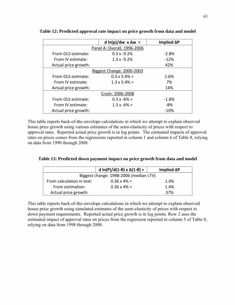
63

Table 12: Predicted approval rate impact on price growth from data and model

d ln(p)/dw x Δw = Implied ΔP Panel A: Overall, 1996‐2006

From OLS estimate: 0.3 x ‐9.2% ‐2.8% From IV estimate: 1.3 x ‐9.2% ‐12% Actual price growth: 42%

Biggest Change: 2000‐2003 From OLS estimate: 0.3 x 5.4% = 1.6% From IV estimate: 1.3 x 5.4% = 7% Actual price growth: 14%

Crash: 2006‐2008 From OLS estimate: 0.3 x ‐6% = ‐1.8% From IV estimate: 1.3 x ‐6% = ‐8% Actual price growth: ‐10%

This table reports back-of-the-envelope calculations in which we attempt to explain observed house price growth using various estimates of the semi-elasticity of prices with respect to approval rates. Reported actual price growth is in log points. The estimated impacts of approval rates on prices comes from the regressions reported in column 1 and column 6 of Table 8, relying on data from 1990 through 2008.

Table 13: Predicted down payment impact on price growth from data and model

d ln(P)/d(1‐θ) x Δ(1‐θ) = Implied ΔP Biggest change: 1998‐2006 (median LTV)

From calculation in text: 0.36 x 4% = 1.4% From estimation: 0.36 x 4% = 1.4%

Actual price growth: 37%

This table reports back-of-the-envelope calculations in which we attempt to explain observed house price growth using simulated estimates of the semi-elasticity of prices with respect to down payment requirements. Reported actual price growth is in log points. Row 2 uses the estimated impact of approval rates on prices from the regression reported in column 5 of Table 8, relying on data from 1998 through 2008.

64

Figure 1: Prices and Interest Rates

Figure 2: Applications and Approval Rate

65

Figure 3: Distribution of Applications

Figure 4: Approval Rates by Demographic Group

66

Figure 5: Measures of Mortgage Approval Rates