Risk Theory and Related TopicsBedlewo, Poland. 28 september- 8 october 2008

1

Credit Default Swaps

Tomasz R. Bielecki, IIT, ChicagoMonique Jeanblanc, University of EvryMarek Rutkowski, University of New South Wales, Sydney

2

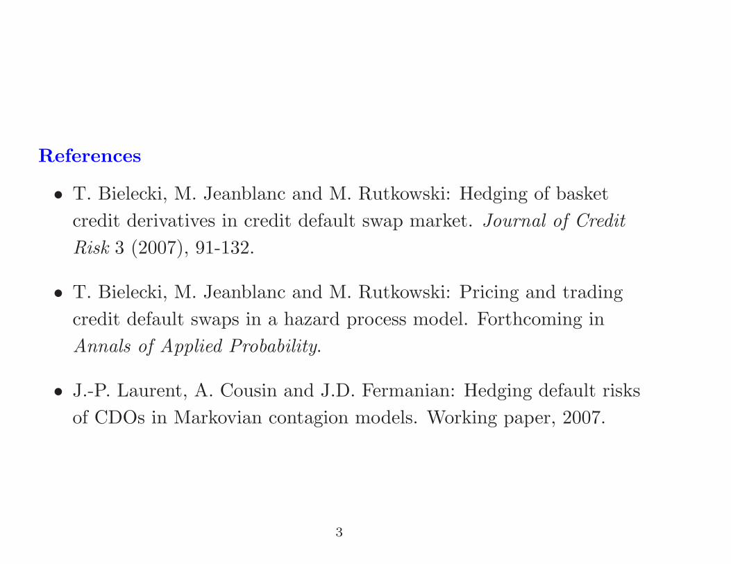
References

• T. Bielecki, M. Jeanblanc and M. Rutkowski: Hedging of basketcredit derivatives in credit default swap market. Journal of CreditRisk 3 (2007), 91-132.

• T. Bielecki, M. Jeanblanc and M. Rutkowski: Pricing and tradingcredit default swaps in a hazard process model. Forthcoming inAnnals of Applied Probability.

• J.-P. Laurent, A. Cousin and J.D. Fermanian: Hedging default risksof CDOs in Markovian contagion models. Working paper, 2007.

3

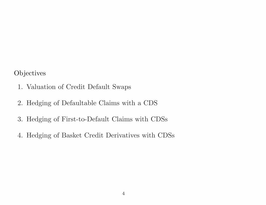
Objectives

1. Valuation of Credit Default Swaps

2. Hedging of Defaultable Claims with a CDS

3. Hedging of First-to-Default Claims with CDSs

4. Hedging of Basket Credit Derivatives with CDSs

4

Credit Default Swaps

Defaultable Claims

A generic defaultable claim (X, A, Z, τ) consists of:

1. A promised contingent claim X representing the payoffreceived by the owner of the claim at time T, if there was no defaultprior to or at maturity date T .

2. A process A representing the dividends stream prior to default.

3. A recovery process Z representing the recovery payoff at time ofdefault, if default occurs prior to or at maturity date T .

4. A default time τ , where the use of the term default is merely aconvention.

5

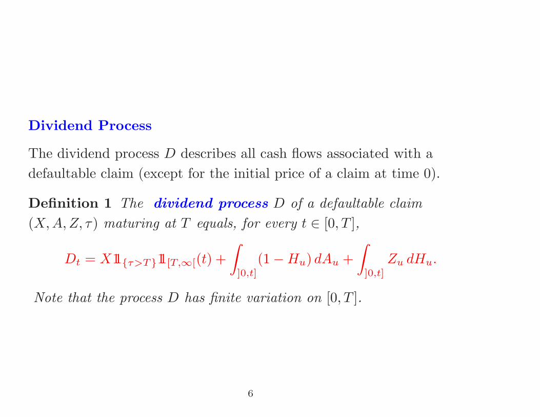
Dividend Process

The dividend process D describes all cash flows associated with adefaultable claim (except for the initial price of a claim at time 0).

Definition 1 The dividend process D of a defaultable claim(X, A, Z, τ) maturing at T equals, for every t ∈ [0, T ],

Dt = X11{τ>T}11[T,∞[(t) +∫

]0,t]

(1 − Hu) dAu +∫

]0,t]

Zu dHu.

Note that the process D has finite variation on [0, T ].

6

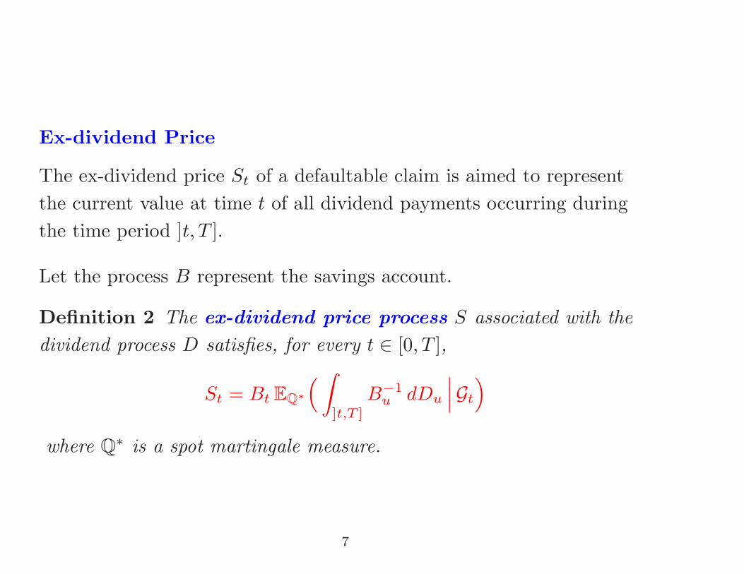
Ex-dividend Price

The ex-dividend price St of a defaultable claim is aimed to representthe current value at time t of all dividend payments occurring duringthe time period ]t, T ].

Let the process B represent the savings account.

Definition 2 The ex-dividend price process S associated with thedividend process D satisfies, for every t ∈ [0, T ],

St = Bt EQ∗(∫

]t,T ]

B−1u dDu

∣∣∣Gt

)where Q∗ is a spot martingale measure.

7

Cumulative Price

The cumulative price St is aimed to represent the current value at timet of all dividend payments occurring during the period ]t, T ] under theconvention that they were immediately reinvested in the savingsaccount.

Definition 3 The cumulative price process S associated with thedividend process D satisfies, for every t ∈ [0, T ],

St = Bt EQ∗(∫

]0,T ]

B−1u dDu

∣∣∣Gt

)= St + Dt

where Dt equals

Dt = Bt

∫]0,t]

B−1u dDu, ∀ t ∈ [0, T ].

8

Credit Default Swap

Definition 4 A (stylized) credit default swap with a constant rate κ

and recovery at default is a claim (0, A, Z, τ), where Z = δ andAt = −κt.

• An F-predictable process δ : [0, T ] → R represents the defaultprotection stream.

• A constant κ represents the CDS spread. It defines the fee leg,also known as the survival annuity stream.

Lemma 1 The ex-dividend price of a CDS maturing at T equals

St(κ) = EQ∗(11{t<τ≤T}δτ

∣∣∣Gt

)− EQ∗

(11{t<τ}κ

((τ ∧ T ) − t

) ∣∣∣Gt

)where Q∗ is a spot martingale measure and B = 1.

9

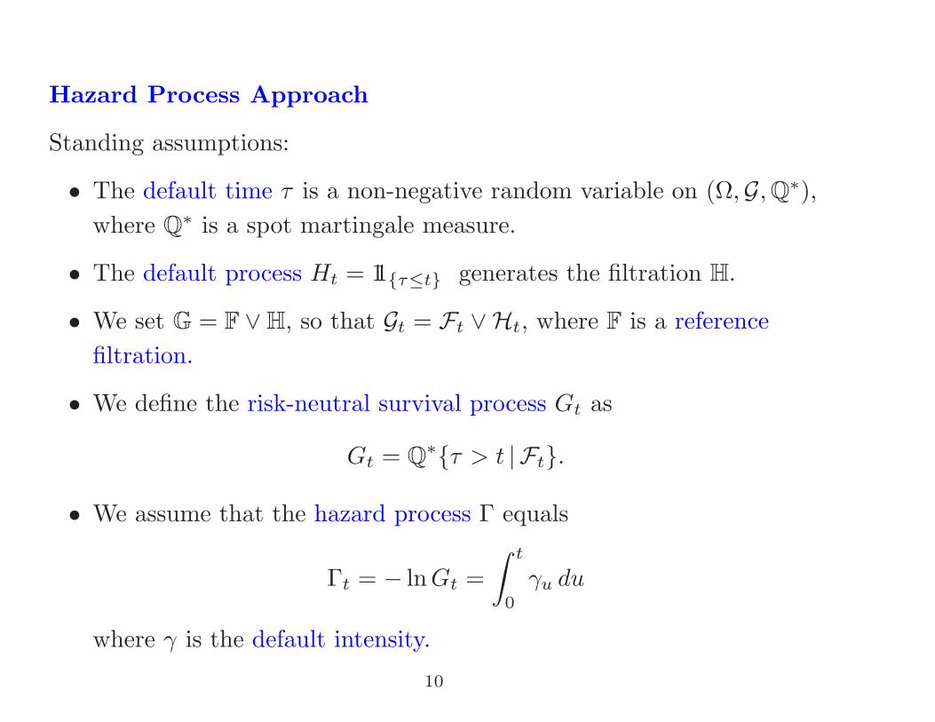
Hazard Process Approach

Standing assumptions:

• The default time τ is a non-negative random variable on (Ω,G, Q∗),where Q∗ is a spot martingale measure.

• The default process Ht = 11{τ≤t} generates the filtration H.

• We set G = F ∨ H, so that Gt = Ft ∨Ht, where F is a referencefiltration.

• We define the risk-neutral survival process Gt as

Gt = Q∗{τ > t | Ft}.

• We assume that the hazard process Γ equals

Γt = − lnGt =∫ t

0

γu du

where γ is the default intensity.

10

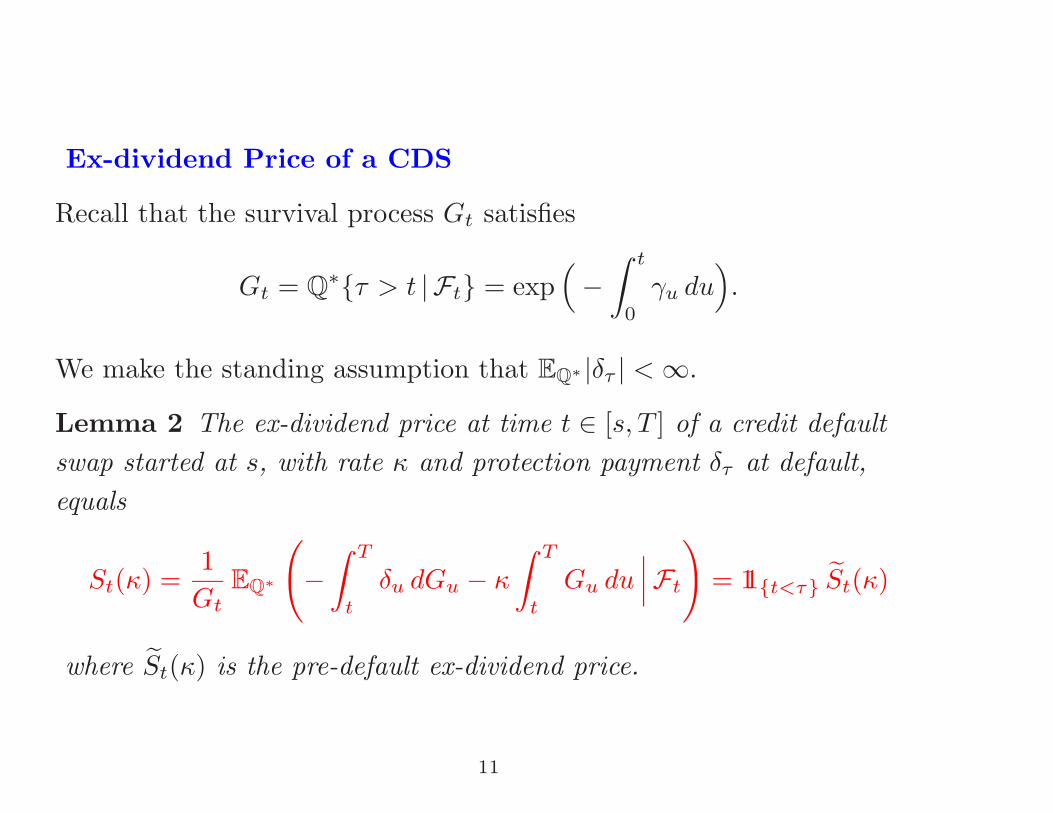
Ex-dividend Price of a CDS

Recall that the survival process Gt satisfies

Gt = Q∗{τ > t | Ft} = exp(−∫ t

0

γu du).

We make the standing assumption that EQ∗ |δτ | < ∞.

Lemma 2 The ex-dividend price at time t ∈ [s, T ] of a credit defaultswap started at s, with rate κ and protection payment δτ at default,equals

St(κ) =1Gt

EQ∗

(−∫ T

t

δu dGu − κ

∫ T

t

Gu du∣∣∣Ft

)= 11{t<τ} St(κ)

where St(κ) is the pre-default ex-dividend price.

11

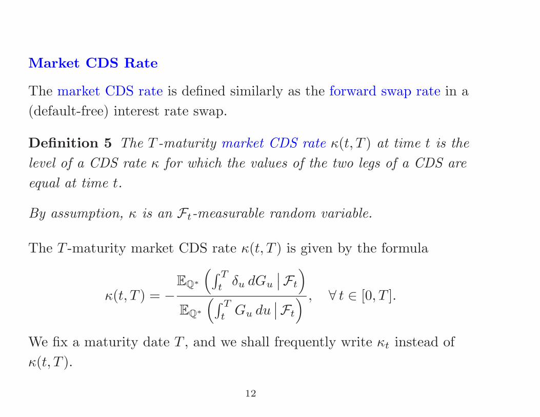
Market CDS Rate

The market CDS rate is defined similarly as the forward swap rate in a(default-free) interest rate swap.

Definition 5 The T -maturity market CDS rate κ(t, T ) at time t is thelevel of a CDS rate κ for which the values of the two legs of a CDS areequal at time t.

By assumption, κ is an Ft-measurable random variable.

The T -maturity market CDS rate κ(t, T ) is given by the formula

κ(t, T ) = −EQ∗

(∫ T

tδu dGu

∣∣Ft

)EQ∗

(∫ T

tGu du

∣∣Ft

) , ∀ t ∈ [0, T ].

We fix a maturity date T , and we shall frequently write κt instead ofκ(t, T ).

12

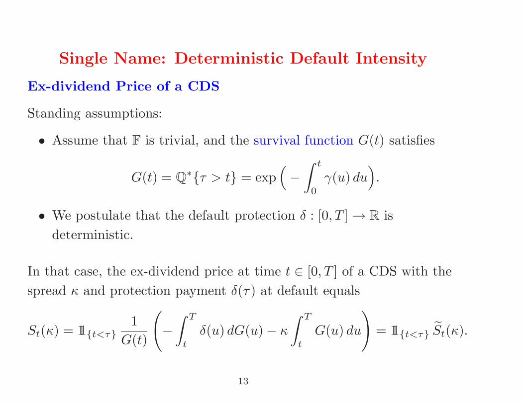
Single Name: Deterministic Default Intensity

Ex-dividend Price of a CDS

Standing assumptions:

• Assume that F is trivial, and the survival function G(t) satisfies

G(t) = Q∗{τ > t} = exp(−∫ t

0

γ(u) du).

• We postulate that the default protection δ : [0, T ] → R isdeterministic.

In that case, the ex-dividend price at time t ∈ [0, T ] of a CDS with thespread κ and protection payment δ(τ) at default equals

St(κ) = 11{t<τ}1

G(t)

(−∫ T

t

δ(u) dG(u) − κ

∫ T

t

G(u) du

)= 11{t<τ} St(κ).

13

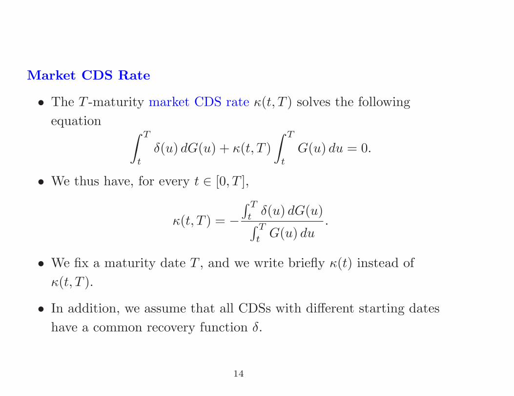
Market CDS Rate

• The T -maturity market CDS rate κ(t, T ) solves the followingequation ∫ T

t

δ(u) dG(u) + κ(t, T )∫ T

t

G(u) du = 0.

• We thus have, for every t ∈ [0, T ],

κ(t, T ) = −∫ T

tδ(u) dG(u)∫ T

tG(u) du

.

• We fix a maturity date T , and we write briefly κ(t) instead ofκ(t, T ).

• In addition, we assume that all CDSs with different starting dateshave a common recovery function δ.

14

Market CDS Rate: Special Case

• Assume that δ(t) = δ is constant, and F (t) = 1 − e−γt for someconstant default intensity γ > 0 under Q∗.

• The ex-dividend price of a (spot) CDS with rate κ equals, for everyt ∈ [0, T ],

St(κ) = 11{t<τ}(δγ − κ)γ−1(1 − e−γ(T−t)

).

• The last formula yields κ(s, T ) = δγ for every s < T , so that themarket rate κ(s, T ) is here independent of s.

• As a consequence, the ex-dividend price of a market CDS started ats equals zero not only at the inception date s, but indeed at anytime t ∈ [s, T ], both prior to and after default).

• Hence, this process follows a trivial martingale under Q∗.

15

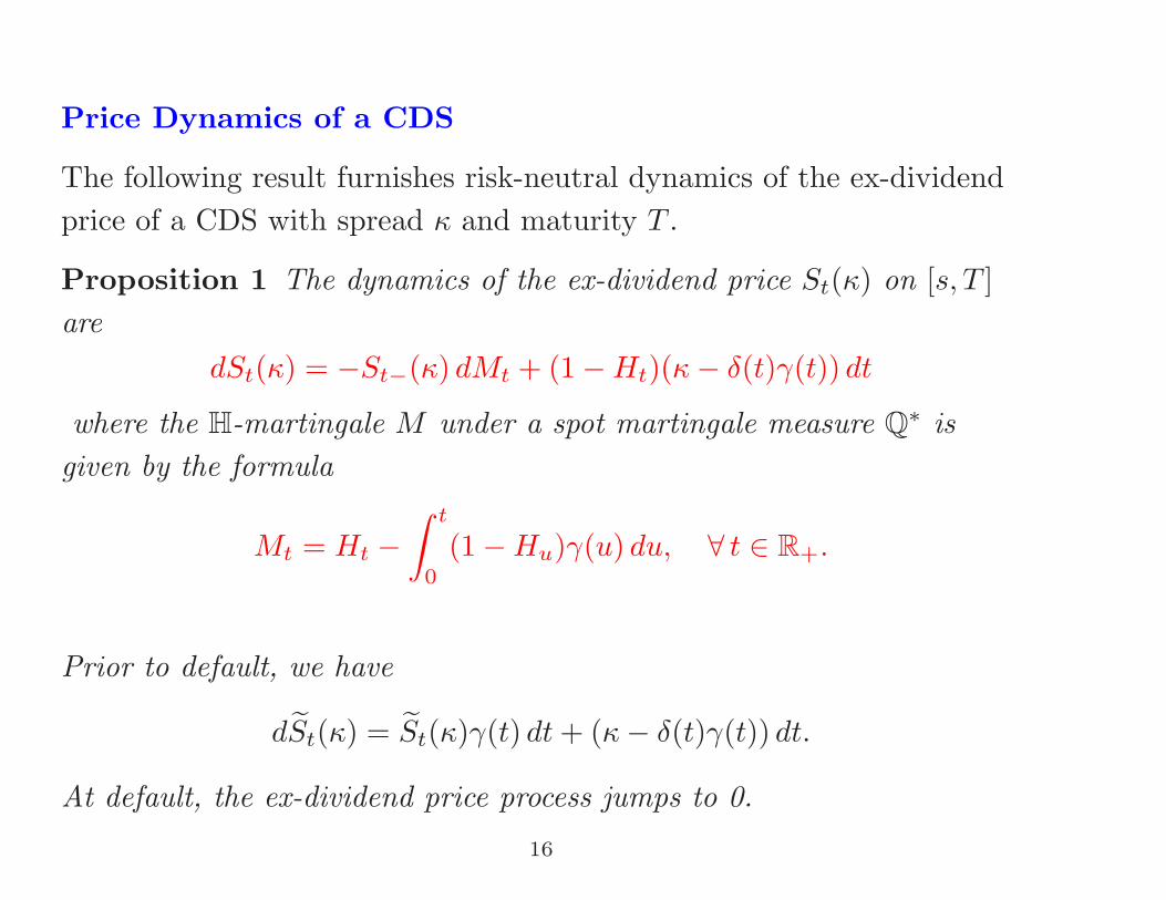
Price Dynamics of a CDS

The following result furnishes risk-neutral dynamics of the ex-dividendprice of a CDS with spread κ and maturity T .

Proposition 1 The dynamics of the ex-dividend price St(κ) on [s, T ]are

dSt(κ) = −St−(κ) dMt + (1 − Ht)(κ − δ(t)γ(t)) dt

where the H-martingale M under a spot martingale measure Q∗ isgiven by the formula

Mt = Ht −∫ t

0

(1 − Hu)γ(u) du, ∀ t ∈ R+.

Prior to default, we have

dSt(κ) = St(κ)γ(t) dt + (κ − δ(t)γ(t)) dt.

At default, the ex-dividend price process jumps to 0.

16

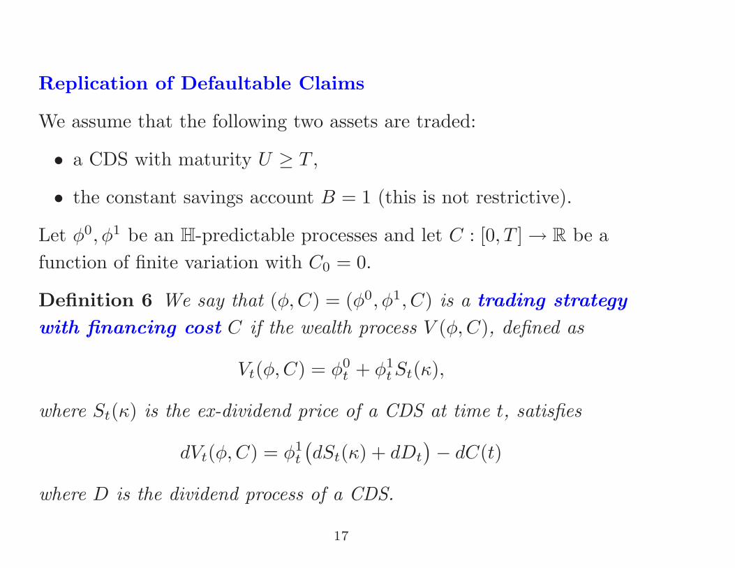
Replication of Defaultable Claims

We assume that the following two assets are traded:

• a CDS with maturity U ≥ T ,

• the constant savings account B = 1 (this is not restrictive).

Let φ0, φ1 be an H-predictable processes and let C : [0, T ] → R be afunction of finite variation with C0 = 0.

Definition 6 We say that (φ, C) = (φ0, φ1, C) is a trading strategy

with financing cost C if the wealth process V (φ, C), defined as

Vt(φ, C) = φ0t + φ1

t St(κ),

where St(κ) is the ex-dividend price of a CDS at time t, satisfies

dVt(φ, C) = φ1t

(dSt(κ) + dDt

)− dC(t)

where D is the dividend process of a CDS.

17

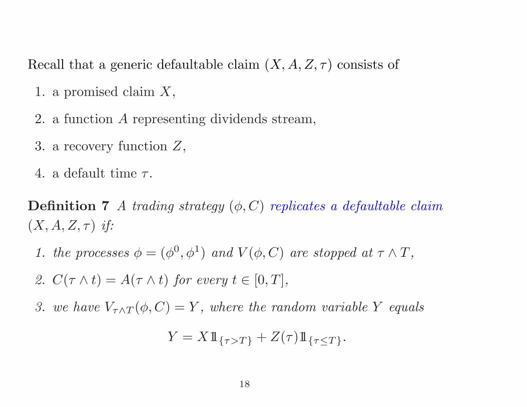
Recall that a generic defaultable claim (X, A, Z, τ) consists of

1. a promised claim X,

2. a function A representing dividends stream,

3. a recovery function Z,

4. a default time τ .

Definition 7 A trading strategy (φ, C) replicates a defaultable claim(X, A, Z, τ) if:

1. the processes φ = (φ0, φ1) and V (φ, C) are stopped at τ ∧ T ,

2. C(τ ∧ t) = A(τ ∧ t) for every t ∈ [0, T ],

3. we have Vτ∧T (φ, C) = Y , where the random variable Y equals

Y = X11{τ>T} + Z(τ)11{τ≤T}.

18

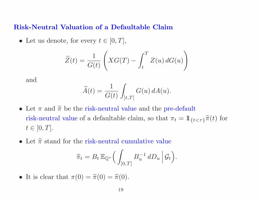
Risk-Neutral Valuation of a Defaultable Claim

• Let us denote, for every t ∈ [0, T ],

Z(t) =1

G(t)

(XG(T ) −

∫ T

t

Z(u) dG(u)

)and

A(t) =1

G(t)

∫]t,T ]

G(u) dA(u).

• Let π and π be the risk-neutral value and the pre-defaultrisk-neutral value of a defaultable claim, so that πt = 11{t<τ}π(t) fort ∈ [0, T ].

• Let π stand for the risk-neutral cumulative value

πt = Bt EQ∗(∫

]0,T ]

B−1u dDu

∣∣∣Gt

).

• It is clear that π(0) = π(0) = π(0).

19

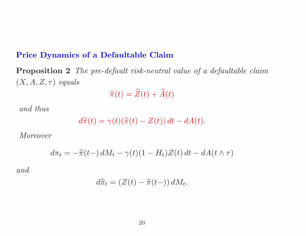
Price Dynamics of a Defaultable Claim

Proposition 2 The pre-default risk-neutral value of a defaultable claim(X, A, Z, τ) equals

π(t) = Z(t) + A(t)

and thusdπ(t) = γ(t)(π(t) − Z(t)) dt − dA(t).

Moreover

dπt = −π(t−) dMt − γ(t)(1 − Ht)Z(t) dt − dA(t ∧ τ)

anddπt = (Z(t) − π(t−)) dMt.

20

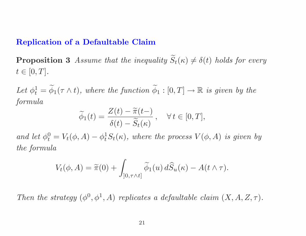
Replication of a Defaultable Claim

Proposition 3 Assume that the inequality St(κ) = δ(t) holds for everyt ∈ [0, T ].

Let φ1t = φ1(τ ∧ t), where the function φ1 : [0, T ] → R is given by the

formula

φ1(t) =Z(t) − π(t−)

δ(t) − St(κ), ∀ t ∈ [0, T ],

and let φ0t = Vt(φ, A) − φ1

t St(κ), where the process V (φ, A) is given bythe formula

Vt(φ, A) = π(0) +∫

]0,τ∧t]

φ1(u) dSu(κ) − A(t ∧ τ).

Then the strategy (φ0, φ1, A) replicates a defaultable claim (X, A, Z, τ).

21

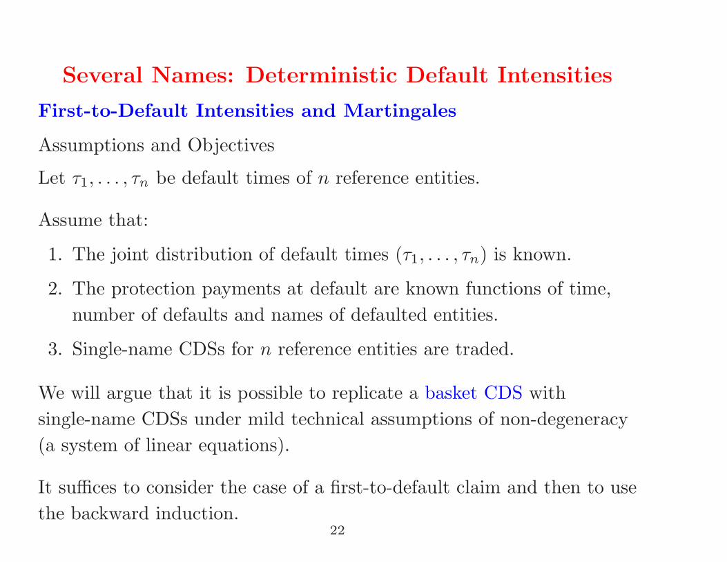
Several Names: Deterministic Default Intensities

First-to-Default Intensities and Martingales

Assumptions and Objectives

Let τ1, . . . , τn be default times of n reference entities.

Assume that:

1. The joint distribution of default times (τ1, . . . , τn) is known.

2. The protection payments at default are known functions of time,number of defaults and names of defaulted entities.

3. Single-name CDSs for n reference entities are traded.

We will argue that it is possible to replicate a basket CDS withsingle-name CDSs under mild technical assumptions of non-degeneracy(a system of linear equations).

It suffices to consider the case of a first-to-default claim and then to usethe backward induction.

22

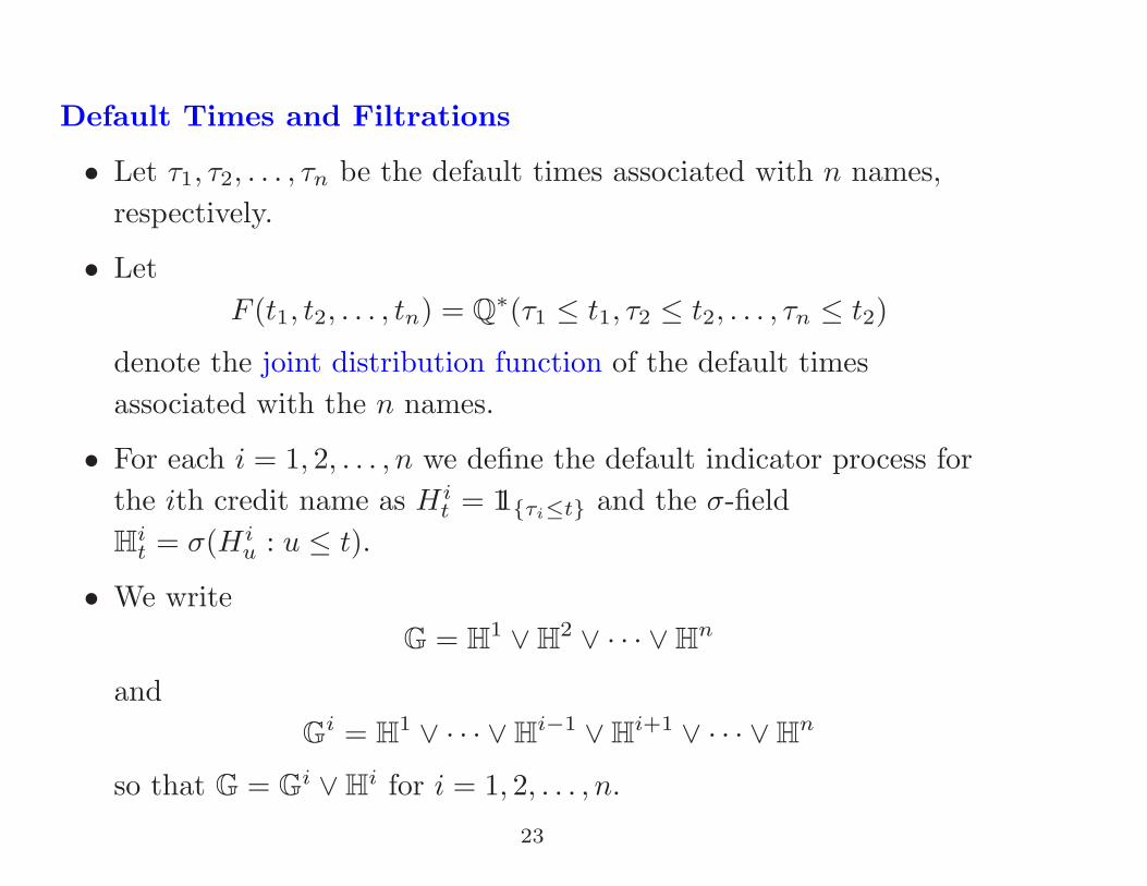
Default Times and Filtrations

• Let τ1, τ2, . . . , τn be the default times associated with n names,respectively.

• LetF (t1, t2, . . . , tn) = Q∗(τ1 ≤ t1, τ2 ≤ t2, . . . , τn ≤ t2)

denote the joint distribution function of the default timesassociated with the n names.

• For each i = 1, 2, . . . , n we define the default indicator process forthe ith credit name as Hi

t = 11{τi≤t} and the σ-fieldHi

t = σ(Hiu : u ≤ t).

• We writeG = H1 ∨ H2 ∨ · · · ∨ Hn

andGi = H1 ∨ · · · ∨ Hi−1 ∨ Hi+1 ∨ · · · ∨ Hn

so that G = Gi ∨ Hi for i = 1, 2, . . . , n.

23

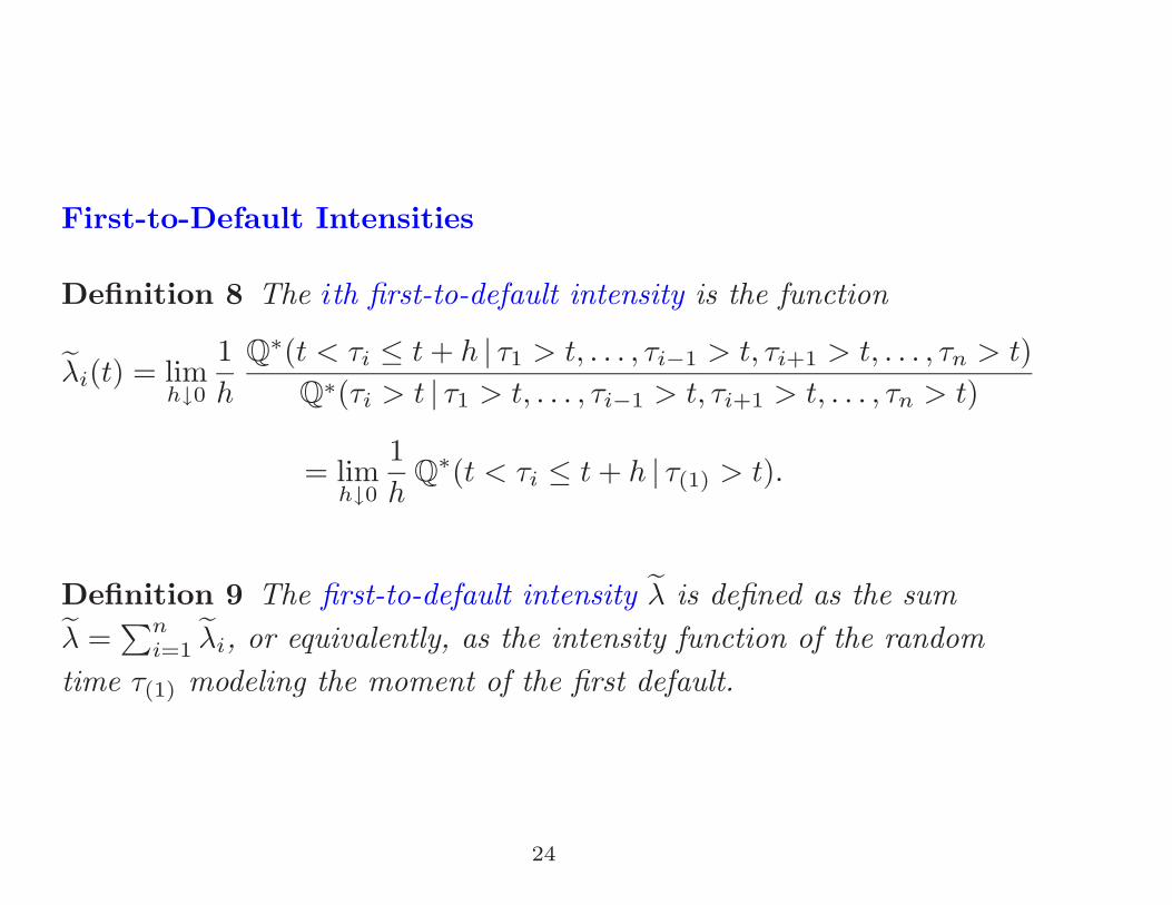
First-to-Default Intensities

Definition 8 The ith first-to-default intensity is the function

λi(t) = limh↓0

1h

Q∗(t < τi ≤ t + h | τ1 > t, . . . , τi−1 > t, τi+1 > t, . . . , τn > t)Q∗(τi > t | τ1 > t, . . . , τi−1 > t, τi+1 > t, . . . , τn > t)

= limh↓0

1h

Q∗(t < τi ≤ t + h | τ(1) > t).

Definition 9 The first-to-default intensity λ is defined as the sumλ =

∑ni=1 λi, or equivalently, as the intensity function of the random

time τ(1) modeling the moment of the first default.

24

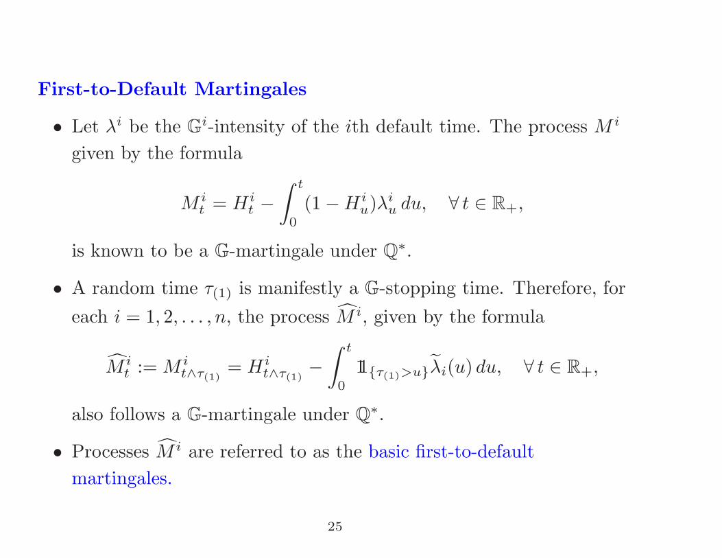
First-to-Default Martingales

• Let λi be the Gi-intensity of the ith default time. The process M i

given by the formula

M it = Hi

t −∫ t

0

(1 − Hiu)λi

u du, ∀ t ∈ R+,

is known to be a G-martingale under Q∗.

• A random time τ(1) is manifestly a G-stopping time. Therefore, foreach i = 1, 2, . . . , n, the process M i, given by the formula

M it := M i

t∧τ(1)= Hi

t∧τ(1)−∫ t

0

11{τ(1)>u}λi(u) du, ∀ t ∈ R+,

also follows a G-martingale under Q∗.

• Processes M i are referred to as the basic first-to-defaultmartingales.

25

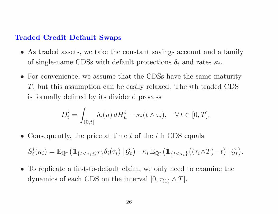
Traded Credit Default Swaps

• As traded assets, we take the constant savings account and a familyof single-name CDSs with default protections δi and rates κi.

• For convenience, we assume that the CDSs have the same maturityT , but this assumption can be easily relaxed. The ith traded CDSis formally defined by its dividend process

Dit =

∫(0,t]

δi(u) dHiu − κi(t ∧ τi), ∀ t ∈ [0, T ].

• Consequently, the price at time t of the ith CDS equals

Sit(κi) = EQ∗

(11{t<τi≤T}δi(τi)

∣∣Gt

)−κi EQ∗(11{t<τi}

((τi∧T )−t

) ∣∣Gt

).

• To replicate a first-to-default claim, we only need to examine thedynamics of each CDS on the interval [0, τ(1) ∧ T ].

26

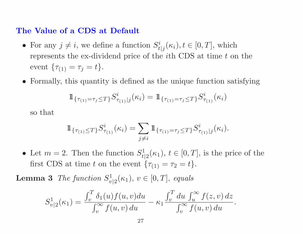
The Value of a CDS at Default

• For any j = i, we define a function Sit|j(κi), t ∈ [0, T ], which

represents the ex-dividend price of the ith CDS at time t on theevent {τ(1) = τj = t}.

• Formally, this quantity is defined as the unique function satisfying

11{τ(1)=τj≤T}Siτ(1)|j(κi) = 11{τ(1)=τj≤T}Si

τ(1)(κi)

so that

11{τ(1)≤T}Siτ(1)

(κi) =∑j �=i

11{τ(1)=τj≤T}Siτ(1)|j(κi).

• Let m = 2. Then the function S1t|2(κ1), t ∈ [0, T ], is the price of the

first CDS at time t on the event {τ(1) = τ2 = t}.Lemma 3 The function S1

v|2(κ1), v ∈ [0, T ], equals

S1v|2(κ1) =

∫ T

vδ1(u)f(u, v)du∫∞v

f(u, v) du− κ1

∫ T

vdu∫∞

uf(z, v) dz∫∞

vf(u, v) du

.

27

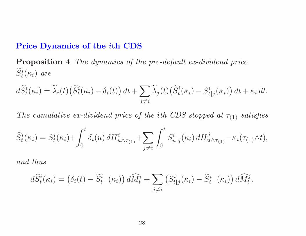
Price Dynamics of the ith CDS

Proposition 4 The dynamics of the pre-default ex-dividend priceSi

t(κi) are

dSit(κi) = λi(t)

(Si

t(κi)− δi(t))dt +

∑j �=i

λj(t)(Si

t(κi)−Sit|j(κi)

)dt + κi dt.

The cumulative ex-dividend price of the ith CDS stopped at τ(1) satisfies

Sit(κi) = Si

t(κi)+∫ t

0

δi(u) dHiu∧τ(1)

+∑j �=i

∫ t

0

Siu|j(κi) dHj

u∧τ(1)−κi(τ(1)∧t),

and thus

dSit(κi) =

(δi(t) − Si

t−(κi))dM i

t +∑j �=i

(Si

t|j(κi) − Sit−(κi)

)dM j

t .

28

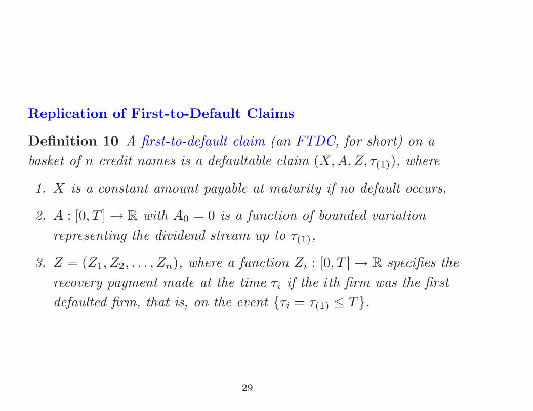
Replication of First-to-Default Claims

Definition 10 A first-to-default claim (an FTDC, for short) on abasket of n credit names is a defaultable claim (X, A, Z, τ(1)), where

1. X is a constant amount payable at maturity if no default occurs,

2. A : [0, T ] → R with A0 = 0 is a function of bounded variationrepresenting the dividend stream up to τ(1),

3. Z = (Z1, Z2, . . . , Zn), where a function Zi : [0, T ] → R specifies therecovery payment made at the time τi if the ith firm was the firstdefaulted firm, that is, on the event {τi = τ(1) ≤ T}.

29

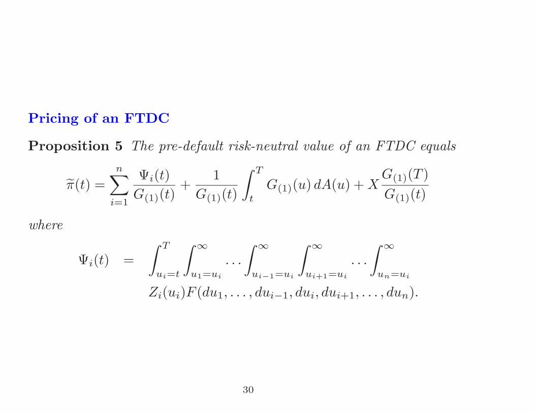
Pricing of an FTDC

Proposition 5 The pre-default risk-neutral value of an FTDC equals

π(t) =n∑

i=1

Ψi(t)G(1)(t)

+1

G(1)(t)

∫ T

t

G(1)(u) dA(u) + XG(1)(T )G(1)(t)

where

Ψi(t) =∫ T

ui=t

∫ ∞

u1=ui

. . .

∫ ∞

ui−1=ui

∫ ∞

ui+1=ui

. . .

∫ ∞

un=ui

Zi(ui)F (du1, . . . , dui−1, dui, dui+1, . . . , dun).

30

Price Dynamics of an FTDC

Proposition 6 The pre-default risk-neutral value of an FTDC satisfies

dπ(t) =∑i=1

λi(t)(π(t) − Zi(t)

)dt − dA(t).

Moreover, the risk-neutral value of an FTDC satisfies

dπt =n∑

i=1

(Zi(t) − π(t−)) dM iu − dA(τ(1) ∧ t),

and the risk-neutral cumulative value π of an FTDC satisfies

dπt =n∑

i=1

(Zi(t) − π(t−)) dM iu.

31

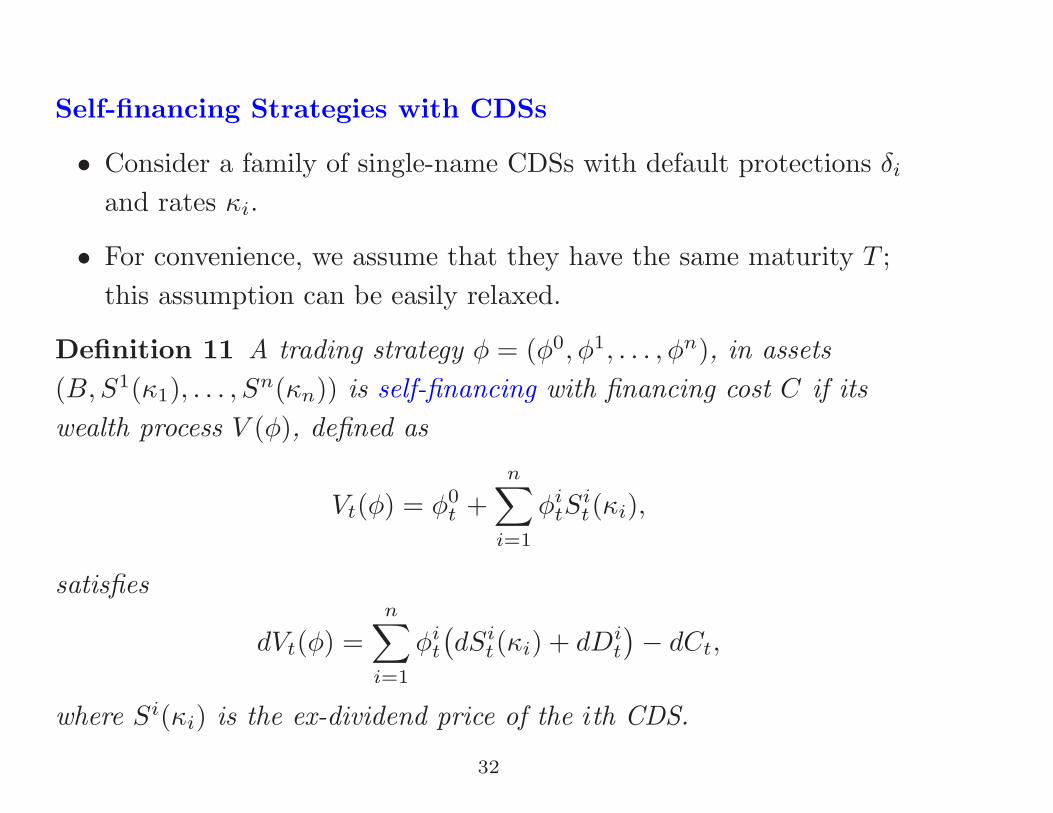
Self-financing Strategies with CDSs

• Consider a family of single-name CDSs with default protections δi

and rates κi.

• For convenience, we assume that they have the same maturity T ;this assumption can be easily relaxed.

Definition 11 A trading strategy φ = (φ0, φ1, . . . , φn), in assets(B, S1(κ1), . . . , Sn(κn)) is self-financing with financing cost C if itswealth process V (φ), defined as

Vt(φ) = φ0t +

n∑i=1

φitS

it(κi),

satisfies

dVt(φ) =n∑

i=1

φit

(dSi

t(κi) + dDit

)− dCt,

where Si(κi) is the ex-dividend price of the ith CDS.

32

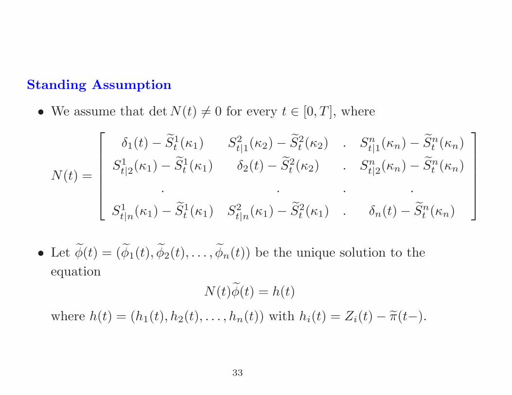
Standing Assumption

• We assume that det N(t) = 0 for every t ∈ [0, T ], where

N(t) =

⎡⎢⎢⎢⎢⎢⎣δ1(t) − S1

t (κ1) S2t|1(κ2) − S2

t (κ2) . Snt|1(κn) − Sn

t (κn)

S1t|2(κ1) − S1

t (κ1) δ2(t) − S2t (κ2) . Sn

t|2(κn) − Snt (κn)

. . . .

S1t|n(κ1) − S1

t (κ1) S2t|n(κ1) − S2

t (κ1) . δn(t) − Snt (κn)

⎤⎥⎥⎥⎥⎥⎦• Let φ(t) = (φ1(t), φ2(t), . . . , φn(t)) be the unique solution to the

equationN(t)φ(t) = h(t)

where h(t) = (h1(t), h2(t), . . . , hn(t)) with hi(t) = Zi(t) − π(t−).

33

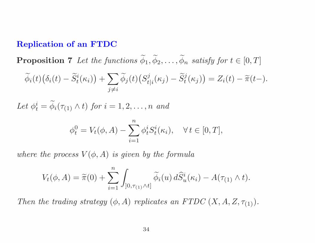
Replication of an FTDC

Proposition 7 Let the functions φ1, φ2, . . . , φn satisfy for t ∈ [0, T ]

φi(t)(δi(t) − Si

t(κi))

+∑j �=i

φj(t)(Sj

t|i(κj) − Sjt (κj)

)= Zi(t) − π(t−).

Let φit = φi(τ(1) ∧ t) for i = 1, 2, . . . , n and

φ0t = Vt(φ, A) −

n∑i=1

φitS

it(κi), ∀ t ∈ [0, T ],

where the process V (φ, A) is given by the formula

Vt(φ, A) = π(0) +n∑

i=1

∫]0,τ(1)∧t]

φi(u) dSiu(κi) − A(τ(1) ∧ t).

Then the trading strategy (φ, A) replicates an FTDC (X, A, Z, τ(1)).

34

Final Remarks

In a single-name case:

• we first considered the case of a default time with a deterministicintensity,

• we have shown that a generic defaultable claim can be replicated bydynamic trading in a CDS and the savings account,

• the extension to the case of non-trivial reference filtration was notpresented.

35

In a multi-name case:

• we first considered the case of a finite family of default times withknown joint distribution,

• the replicating strategy for a first-to-default claim was examined;the method can be extended to kth-to-default claims,

• in the next step, the approach was extended to the case of areference filtration generated by a multi-dimensional Brownianmotion.

36