Unobservable Selection and Coefficient Stability:

Theory and Evidence∗

Emily Oster

Brown University and NBER

November 24, 2014

Abstract

A common heuristic for evaluating robustness of results to omitted variable bias is to observe coefficientmovements after inclusion of controls. This heuristic is informative only if selection on observables isinformative about selection on unobservables. I formalize this link through a proportional selectionassumption. I show that it is necessary to take into account coefficient movements and movements inR-squared values in identifying omitted variable bias. I further demonstrate that in the empiricallycommon case with multiple observed controls it is also necessary to account for the share of the variation intreatment accounted for by control variables. I describe a formal bounding argument for omitted variablebias under the proportional selection assumption. I show two validation exercises suggesting that thisperforms well empirically. I discuss application of this procedure to a large set of publications in economics,and use evidence from randomized studies to draw guidelines for bounding values.

∗Ling Zhong, Unika Shrestha, Damian Kozbur, Guillaume Pouliot, David Birke and Angela Li provided excellent researchassistance. I thank David Cesarini, Raj Chetty, Todd Elder, Amy Finkelstein, Guido Imbens, Larry Katz, Matt Gentzkow,Matt Notowidigdo, Chad Syverson, Manisha Shah, Azeem Shaikh, Jesse Shapiro, Bryce Steinberg, Matt Taddy, Heidi Williamsand participants in seminar at Brown University, University of Chicago Booth School of Business, Wharton and Yale for helpfulcomments. I am grateful to a number of authors for providing replication files or re-running analysis by request. I gratefullyacknowledge financial support from the Neubauer Family. Stata code to preform the calculations described in this paper is availablefrom the authors website or through ssc under the name psacalc.

1

1 Introduction

Concerns about omitted variable bias are common to most or all non-experimental work in economics.1 The

most straightforward approach to such concerns is to include controls which can be observed. Angrist and

Pischke (2010) argue that among the major advances in empirical economics in the past two decades is greater

effort to identify the most important threats to validity, and to address them with appropriate selection of

controls. Even with careful selection of controls, however, the possibility of bias from unobserved controls

remains.

A common heuristic for evaluating the robustness of a result to omitted variable bias concerns is to look

at the sensitivity of the treatment effect to inclusion of observed controls. In three top general interest

economics journals in 2012, 75% of non-experimental empirical papers included such sensitivity analysis.2 The

intuitive appeal of this approach lies in the idea that the bias arising from the observed controls is informative

about the bias that arises from the unobserved ones. This is not, however, implied by the baseline assumptions

underlying the linear model.

Formally, using the observables to identify the bias from the unobservables requires making further

assumptions about the covariance properties of the two sets. One one extreme, if the unobservables are

completely unlike the observables, nothing about the remaining bias is learned from the inclusion of the

observables. The case in which the bias is fully identified is the other extreme: where one assumes all of the

unobservables share the same covariance properties as the observables (Murphy and Topel, 1990; Altonji,

Elder and Taber, 2005; Altonji et al, 2011).

Even under this most optimistic assumption, however, coefficient movements alone are not a sufficient

statistic to calculate bias. To illustrate why, consider the case of a researcher estimating wage returns to

education with individual ability as the only confound (this example is motivated by independent work by

Pischke and Schwandt (2013)). Assume wages would be fully explained if an exact measure of ability could be

observed but, in practice, the researcher sees only an imprecise ability proxy. As the precision of the ability

control declines, the coefficient will become more stable. This is not because the bias is smaller, but simply

because much of the added control is noise.

This example is described in more detail in Section 2. The key observation is that the quality of the

control will be diagnosed by the movement in R-squared when the control is included. This observation

generalizes to all cases in which the observed controls share covariance properties with the unobserved

1Despite recent trends, this still makes up the vast majority of results within economics: in 2012 the combination of theAmerican Economic Review, the Quarterly Journal of Economics and the Journal of Political Economy published 69 empirical,non-structural papers, only 11 of which were randomized.

2The sample includes non-structural papers in the American Economic Review, Journal of Political Economy and QuarterlyJournal of Economics. The link between coefficient stability and omitted variable bias is often quite direct. For example, Chiapporiet al (2012) state: “It is reassuring that the estimates are very similar in the standard and the augmented specifications, indicatingthat our results are unlikely to be driven by omitted variables bias.” Similarly, Lacetera et al (2012) state: “These controls do notchange the coefficient estimates meaningfully, and the stability of the estimates from columns 4 through 7 suggests that controllingfor the model and age of the car accounts for most of the relevant selection.”

2

controls. Omitted variable bias is proportional to coefficient movements, but only if such movements are scaled

by movements in R-squared. This point is closely related to the partial R-squared logic in Imbens (2003).

The importance of R-squared movements is rarely acknowledged in discussions of coefficient stability. In

Section 2 I demonstrate this using a sample of 57 top journal papers in economics which present coefficient

stability evidence. Only 5 mention anything about R-squared movements and 30% do not even report

R-squared values. Moreover, there is little relationship between the change in coefficient and the change in

R-squared, suggesting that coefficient movements alone are not diagnosing bias. As a further point, the basic

underlying assumption of proportional selection, which is required for coefficient movements to have any

relation with bias, is typically neither acknowledged or tested.

This paper develops a formal approach to robustness based on coefficient stability. I make explicit the

link between coefficient movements, R-squared movements and omitted variable bias through the assumption

of related covariance. I suggest a structured notion of robustness. I perform two validation examples - one

based on constructed data and one linking possibly biased observational relationships to external causal

estimates - which suggest this procedure performs well. Finally, I apply this adjustment to a set of papers in

economics and use insights from randomized data to suggest standards for robustness.

I begin in Section 3 with the theory. To facilitate intuition, I first develop the estimator under the

assumption that there is a single observable control and equal selection on observed and unobserved variables.

Formally, I consider the following model Y = βX + γ1wo1 +W2 + ε, where W2 is unobserved and therefore

cannot be included in the estimation. I impose the equal selection assumption:Cov(γ1w

o1 ,X)

V ar(γ1wo1) = Cov(W2,X)V ar(W2) . This

echoes the setup from Altonji, Elder and Taber (2005). Under this assumption, the omitted variable bias on

the treatment effect estimated with controls can be expressed as an intuitive function of the coefficient and

R-squared values. In particular, the residual omitted variable bias after inclusion of controls is proportional to

the coefficient movements and the ratio of the movement in R-squared with inclusion of the observable control

to the expected movement in R-squared with the inclusion of the unobservable controls.

I then develop a general estimator for the bias when there are multiple observed controls. In most

empirical settings researchers include multiple observed controls in their regressions, so this generalization is a

crucial one for empirical applications. I also relax the assumption of equal selection and replace it with a

proportional selection assumption in which the covariance relationship above is proportional, not necessarily

equal, and relies on a coefficient of proportionality, δ. The estimator in this case can be expressed as a function

of δ, the coefficient and R-squared movements, as well as information on the variance of the treatment and the

share of that variance that is explained by the observed controls. In many cases, the simple estimator

developed first will provide a close approximation to the general estimator, suggesting intuition about the bias

can be easily developed from coefficient and R-squared movements. However, this is not always true.

Importantly, it is possible in the case with multiple controls that the coefficient will appear stable - may even

3

be completely unchanged - and there may still be large bias on the estimated treatment effect.

A key input into either estimator is the R-squared from a hypothetical regression of the outcome on

treatment and both observed and unobserved controls; I denote this Rmax. If the outcome can be fully

explained by the treatment and full controls set, then Rmax = 1. This is the assumption that Altonji, Elder

and Taber (2005) adopt. In many empirical settings it seems likely (due, for example, to measurement error)

that the outcome cannot be fully explained even if the full control set were included. Knowledge about

measurement error or expected idiosyncratic variation in the outcome can be used to develop intuition about

this value.

Following the theory I discuss implementation, with the goal of suggesting a formal expression of

robustness that might replace heuristic statements about small coefficient movements. As in Altonji, Elder

and Taber (2005) I suggest that equal selection (i.e. δ = 1) may be an appropriate upper bound on δ.

Essentially, this argues that the unobservables should not be more important than the observables in

explaining the treatment. I then suggest that researchers adopt a bounding value for Rmax - ideally a

conservative upper bound, denoted Rmax - and report either the value of δ for which the estimator would

produce a treatment effect of zero or the value of β which is produced by δ = 1 and Rmax. In the former case,

a value of δ > 1 would be seen as suggesting a robust results; in the latter, showing that the adjusted β leads

to the same conclusion would be a natural standard. The latter essentially argues for the construction of an

“identified set”, akin to the logic in Tamer (2010) and Manski (2003), bounded on one side by the controlled

treatment effect and on the other by the bias-adjusted effect with δ = 1 and Rmax = Rmax.

I then turn to testing the performance of the estimator in data and, by extension, testing the underlying

proportional selection assumption.

Section 5 first uses NLSY data to construct a dataset relating education and wages; the data is

constructed such that we know the true treatment effect. I evaluate the performance of this adjustment by

excluding combinations of controls from the “observed” set. I estimate the value of δ which would be produced

by each excluded set and calculated the bias-adjusted treatment effect. I show in 89% of cases using the

bounding logic described in above would produce a set which includes the true effect; in only 62% of cases

does the confidence interval of the naive controlled coefficient include this effect. This may actually undervalue

this performance as the control set is selected here at random rather than based on using the most important

controls first, as would be common in practice. I show in this case that approximating the general estimator

with the simple estimator would make little difference to the conclusions.

In a second test I estimate several relationships between maternal behavior and child outcomes;

socioeconomic status confounds are a major concern. I match possibly biased observational estimates with

external evidence on causal effects from randomized data or comprehensive meta-analyses (this is close in

spirit to Lalonde (1986)). I then ask whether the robustness tests described above would separate true from

4

false associations. I find that the adjustment performs well: the approach identifies as robust only the two

relationships for which external evidence confirms a link. I find that in this case the simple approximation

would perform less well and substantially understates the bias in some relationships.

Both of the validation exercises suggest empirical support for this assumption.

In the final section of the paper I turn to the application of this procedure to the economics literature. I

focus on two questions: (1) How do stability statements in published papers in economics hold up to a version

of this adjustment?; (2) Is it possible to make a general statement about bounds on Rmax?

I begin with a sample of papers in the American Economic Review, Journal of Political Economy,

Quarterly Journal of Economics and Econometrica, published between 2008 and 2013 and satisfying a set of

citation cutoffs. I extract all relationships for which a coefficient stability heuristic is reported (57 papers; 131

results). I limit to cases where it is possible to access replication files, which is necessary for calculating some

of the inputs; this limits the sample to 89 results. I calculate the bias-adjusted treatment effect with δ = 1 and

varying bounding values for Rmax. My primary definition of robustness is whether this exercise rejects zero; I

also explore an auxiliary definition related to coefficient size.

Only about 20% of results are robust to a value of Rmax = 1. I show other bounds on Rmax which are a

function of the fully controlled R-squared. These capture the idea that there is variation in how predictable

outcomes are, and this variation can be roughly inferred from how much is predicted by the observables.

Denoting the fully controlled R-squared as R, I explore robustness to Rmax = ΠR, with varying values of Π.

About 37% of results are robust to a value of Π = 2, and 66% to a value of Π = 1.25.

I compare the conclusions from the general estimator to the simple approximation. Eighty percent of

the time the simple approximation would lead to the same conclusions, although the error is sometimes

sizable. In 90% of cases the simple approximation understates the bias, on average by around 30%. This

points to the importance of performing the full bias calculation.

There is considerable variation across papers in the robustness of these stability claims, but this does

not suggest an appropriate general value for the bound on Rmax. For that, I turn to randomized results. The

claim that the coefficient is unchanged by inclusion of controls implicitly suggests that the treatment is

assigned as if randomly. If that is the case, then the coefficient movement should be within the bounds we

would see if treatment were randomized. It is common in randomized papers to show coefficients with and

without controls, either as a balancing test or to increase precision.

I draw a sample of all randomized papers from the American Economic Review, Journal of Political

Economy, Quarterly Journal of Economics, Econometrica and American Economic Journal: Applied

Economics between 2008 and 2013 which report coefficients with and without controls and for which I can

access replication files (65 results). I derive cutoffs based on values of Π which would allow 90% of randomized

results to survive: this value is Π = 1.3.

5

This provides a full robustness reporting standard. I suggest that researchers either (1) report the value

of δ for which β = 0 with Rmax = 1.3R and show it exceeds 1 or; (2) calculate the bias-adjusted β with δ = 1

and Rmax = 1.3R and show it leads to the same conclusion.

In the full sample of non-randomized results considered, about 54% would survive this bounding

robustness argument. I conclude this section by discussing some examples which illustrate the importance of

both taking into account the movement in R-squared and consider the full estimator rather than just the

sample approximation.

This paper adds to a large literature on causal inference in the face of unobserved confounds

(Rosenbaum and Rubin, 1983). Imbens (2003) presents an analysis of sensitivity using a partial R-squared

logic which is conceptually similar to the insights here. A number of methodological papers consider the

approach of varying the covaraite set as a sensitivity analysis (Heckman and Holz, 1989; Dehejia and Wahba,

1999). In the formal use of the proportional selection assumption I follow several recent papers (Murphy and

Topel, 1990; Altonji, Elder and Taber, 2005; Altonji et al, 2011). I add to this literature first by connecting

more explicitly with the intuitive methodologies used by many empirical researchers in evaluating bias, and by

connecting the theory directly to empirical work. From a theoretical standpoint the most significant

contribution is to provide a formal estimator for the bias in a general case. To my knowledge this has not been

done before.3

The rest of the paper is organized as follows. Section 2 provides an illustrative example of the issues

raised above and describes the use of coefficient stability heuristic in economies. Section 3 describes the theory

and Section 4 briefly discusses implementation. Section 5 performs the validation tests and Section 6 turns to

the applications within economics. Section 7 concludes.

2 Coefficient Stability Heuristic: Illustrative Example and Use in

Economics

I motivate the analysis in the paper with a simple illustration of the issues here, and with some data on

coefficient stability within economics.

Illustrative Example

A central point of this paper is to make clear that coefficient movements alone are not sufficient to discuss

bias, even under the strong assumption of related observed and unobserved variables. As an illustration,

consider the case of a researcher estimating wage returns to education with individual ability as the only

3Altonji, Elder and Taber (2005) provide a system for calculating δ under the null that β = 0. Under this assumption the issueof multiple versus single controls is moot becaue it is possible to observe the true index of controls in a regression of treatment onobserved controls.

6

confound (this example is motivated by independent work by Pischke and Schwandt (2013)). Assume wages

would be fully explained if an exact measure of ability could be observed but, in practice, the researcher sees

only an imprecise ability proxy. As the precision of the ability control declines, the coefficient will become

more stable. This is not because the bias is smaller, but simply because much of the added control is noise.

To see this precisely, consider Panel A of Table 1. This panel uses constructed data in which the true

treatment effect is zero and there is a single confound. The first row shows controlled and uncontrolled

coefficients when the observed control is a precise measure of the true confound; the second shows the

coefficients when the observed control is very imprecise. The coefficient in the second row appears much more

stable, even though the true effect is zero in both.

The key difference in the two rows is the change in R-squared, which diagnoses the poor quality of the

proxy in the second row compared to the first. The uninformative control leaves the coefficient largely

unchanged but also adds little to the R-squared. This observation generalizes to all cases in which the

observed controls share covariance properties with the unobserved controls. Omitted variable bias is

proportional to coefficient movements, but only if such movements are scaled by movements in R-squared.

The converse of this point in made in Panel B. Here, I consider two constructed examples in which the

coefficient movement is identical but the movements in R-squared vary widely. In the first row, the small

coefficient movement is accompanied by a large move in R-squared; in the second row, the move in R-squared

is very small. To the extent that we would like to draw conclusions about the true treatment effect from the

controlled coefficient, our intuition suggests that we will come closer in the first case than the second. The fact

that so much of the outcome is explained in the controlled regression suggests that there is simply very little

variation left to bias the coefficient.

Indeed, if we assume that in both cases the observed and unobserved variables would together explain all

of the variation in Y and these two sets relate to the treatment X in the same way (this is the equal selection

assumption discussed much more below) the final column of Panel B shows the implied true treatment effect.

Clearly it is only in the first row that reasonable conclusions could be drawn based on the controlled coefficient.

Coefficient Stability in Economics

The discussion above makes clear the importance of incorporating movements in R-squared in coefficient

stability discussions. In empirical work in economics, however, the importance of the R-squared movements

are rarely acknowledged in these discussions.

To elaborate on this claim, I extract all papers in the American Economic Review, Quarterly Journal of

Economics, The Journal of Political Economy and Econometrica from 2008-2010 with at least 20 citations in

the ISI Web of Science, and those from 2011-2013 in the same journals with at least 10 citations. From these

papers I extract all results where the researcher explores the sensitivity of the result to a control set. This

7

sample (full citation list in Appendix D) includes 57 papers with 131 total results. Only 5 of these papers

mention anything about R-squared movements, and 29% of them do not report the R-squared values in the

paper.

In principle, if coefficients and R-squared values typically move together, it is possible this omission

would not meaningfully affect conclusions. That is, if large coefficient movements are always accompanied by

large R-squared movements, then the coefficient stability is effectively a sufficient statistic. Similarly, if the

controlled R-squared values are always very large - say, always close to 1 - then the coefficient movements

would be enough. In practice, neither of these is the case.

Figure 1 uses the results extracted from the 57 papers described above.4 I limit the sample to results

where the controlled effect is significant. The figures graph the relationship between the percent movement in

effect size and the absolute movement in R-squared values. Figure 1a uses all results, and Figure 1b limits to

cases where the inclusion of controls moves the coefficient toward zero.

It is not the case that the controlled regressions uniformly have a high R-squared. The range of values

for the controlled R-squared are 0.0005 to 0.9894, with an average of 0.42. Moreover, there at best a very weak

relationship between coefficient movements and R-squared movements. If we limit to results where the percent

change in coefficient values is between -12% and -8%, the range of changes in R-squared values is from 0.008 to

0.29.

To develop one concrete comparison, we can consider points (A) and (B) in Figure 1b. In the result in

point (A), the coefficient decreases from 0.49 to 0.43 with inclusion of controls, and the R-squared increases

from 0.44 to 0.93. In the result in point (B), the coefficient change is in a similar range - from 0.21 to 0.19 -

but the increase in R-squared is only 0.36 to 0.37. These sets of figures could have very different implications

for the true treatment effect. If we assume that in both cases the observed and unobserved variables would

together explain all of the variation in Y and these two sets relate to the treatment X in the same way, the

true treatment effect for point (A) is 0.42, whereas the true effect for point (B) is -1.23.

The remainder of this paper develops an estimator for bias under the proportional selection assumption.

This will provide a formal way to relate coefficient and R-squared movements to omitted variable bias. This

formal development will also lay bare a second issue. When there are multiple controls included (as is common

in most applications) coefficient stability may be misleading even in the presence of sizable R-squared

movements. This provides a stronger argument for presenting formal results on bias adjustment rather than

relying on heuristic statements.

In the final section of the paper I will return to the economics literature and revisit these data and

results in light of the estimator developed.

4In the 29% of cases where R-squared was not reported I use replication files to estimate or request these from the researcher.In 2 cases it was not possible to obtain R-squared values.

8

3 Theory

I begin in this section by developing the simple case of a single observable variable and equal selection on

observed and unobserved variables. The solution in this case is intuitive. The second subsection derives and

discusses the general estimator, including a brief discussion of inference. The third subsection discusses the

relation between the two estimators.

3.1 Single Observable, Equal Selection

Consider the regression model

Y = βX + γ1wo1 +W2 + ε (1)

X represents the treatment and the coefficient of interest is β; wo1 and W2 represent confounders. Specifically,

wo1 is an observed control variable with true coefficient γ1. W2 is a vector which is a linear combination of

unobserved control variables wuj , multiplied by their true coefficients: W2 =∑Juj=1 w

uj γ

uj . Define W1 = γ1w

o1.

W1 is therefore an index of the observed control multiplied by its true coefficient. I assume that ε is orthogonal

to X, wo1 and W2.

I assume that Cov(W1,W2) = 0 and that V ar(X) = σXX . The assumption of orthogonality between W1

and W2 is discussed in more detail below. The covariance matrix associated with the vector [X,W1,W2]′ is

positive definite. Note that without further assumptions on the relationship between X, wo1 and W2 there is no

information provided about the bias associated with W2 by seeing the bias from wo1.

Define the equal selection relationship as σ1X

σ11= σ2X

σ22, where σiX = Cov(Wi, X), σii = V ar(Wi). Note

this relationship is defined on the index W1, not directly on the variable wo1.

Define the coefficient resulting from the short regression of Y on X as β and the R-squared from that

regression as R. Define the coefficient from the intermediate regression of Y on X and wo1 as β and the

R-squared as R. Finally, define Rmax as the R-squared from a hypothetical regression of Y on X, wo1 and W2.

Note these are in-sample values.

The omitted variable bias on β and β is controlled by the auxiliary regressions of (1) wo1 on X; (2) W2

on X; and (3) W2 on X and wo1. Denote the in-sample coefficient on X from regressions of wo1 and W2 on X as

λwo1 |X and λW2|X , respectively and the coefficient on X from a regression of W2 on X and wo1 as λW2|X,wo1 .

Denote the population analogs of these values λwo1 |X , λW2|X and λW2|X,wo1 .

All estimates are implicitly indexed by n. Probability limits are taken as n approaches infinity. All

observations are independent and identically distributed according to model (1). By standard omitted variable

bias formulas, I can express the probability limits of the short and intermediate regression coefficients in terms

9

of these values:

βp→ β + γ1λwo1 |X + λW2|X

βp→ β + λW2|X,wo1

The asymptotic bias on β (the coefficient on X with controls included) is λW2|X,wo1 which, given the definitions

above, is equal to σ22σ1X

σ11(σXX−σ21Xσ11

). Denote this bias as Π.

Define the following.

β∗ = β −[β − β

] Rmax − RR− R

Proposition 1 summarizes the result.

Proposition 1. β∗p→ β.

Proof. I outline the proof here, with details in Appendix A.1. Using the definition of coefficient and R-squared

values and recalling the bias is denoted Π we have the following relationships.

(β − β)p→

(σ1X

σXX

)(1− σ1X

σ11Π

)(R− R

)σyy

p→ σ11 + Π2(σXX −σ2

1X

σ11)− 1

σXX

(σ1X + Π(σXX −

σ21X

σ11)

)2

(Rmax − R)σyyp→ Π

σ11

(σXX − σ2

1X

σ11

)σ1X

−Π

(σXX −

σ21X

σ11

)These define a system of three equations in three unknowns (σ11,σ1X and Π). The system is identified and the

solution is Π =[β − β

]Rmax−RR−R .

Some intuition for this result may be developed by observing that Π = β − β so this result implies that

β−ββ−β

= Rmax−RR−R . That is, under the equal selection assumption the ratio of the movement in coefficients is

equal to the ratio of the movement in R-squared. The objects W1 and W2 enter the equation for Y

symmetrically in terms of coefficients, and equal selection implies they also are symmetric in their impact on

X. The only way in which their impact may differ is if they have different variances. This possible difference

will be captured in the differential contributions to R-squared. In the special case where the variances are

equal, then Rmax−RR−R = 1 and the coefficient movement with inclusion of observed controls is equal to the

expected coefficient movement with unobserved controls.5

It is important to note that the setup and result here is exactly what we would derive if we were able to

observe W1 directly, rather than wo1. This is because the coefficient and R-squared values from the short and

intermediate regressions are the same in either case.

5This is the special case dealt with in Bellows and Miguel (2009).

10

Proportional Selection

Define the proportional selection relationship as δ σ1X

σ11= σ2X

σ22, where δ is the coefficient of proportionality.

Equal selection corresponds to the case of δ = 1. With δ 6= 1 the estimator β∗ = β − δ[β − β

]Rmax−RR−R will be

a close approximation for the bias as long as δ is relatively close to 1. This observation leads to the possibility

of calculating an approximate value for δ which is the degree of selection for which β is equal to some target

value β; when β = 0 this tells us the degree of selection on unobservables relative to observables which would

be sufficient to explain away the result. Specifically, δ ≈ (β−β)(R−R)(β−β)(Rmax−R)

.

For the case where β = 0 this is equivalent to the estimator developed in Altonji, Elder and Taber

(2005) and is consistent under the null that β = 0.

3.2 General Estimator

I consider now the general case where selection is proportional and there are possibly multiple variables in the

set of observable controls. I retain much of the notation from above and the proof method proceeds similarly.

Consider the regression model

Y = βX + Ψωo +W2 + ε (2)

where ωo is a vector of the observed controls, ωo1...ωoj . The index W2 is not observed. Define W1 = Ψωo and

assume that all elements of ωo are orthogonal to W2, so W1 and W2 are orthogonal. Without loss of generality,

assume the elements of ωoare also orthogonal to each other.6 Define the proportional selection relationship as

δ σ1X

σ11= σ2X

σ22, where σiX = Cov(Wi, X), σii = V ar(Wi) and δ is the coefficient of proportionality. Note that at

this point we do not make any assumptions about δ so this relationship will always hold for some δ.

The orthogonality of W1 and W2 is central to deriving the results here and maybe some what at odds

with the intuition that the observables and the unobservables are “related”. In practice, the weight of this

assumption is in how we think about the proportionality condition. To see that, consider the case where the

elements of ωo are correlated with W2. The coefficient of proportionality is some δ1. Now define W2 as the

residual from a regression of W2 on ωo. By definition W2 is orthogonal to ωo and all the coefficients and

R-squared values defined below will be identical to the original setup. The coefficients on the elements of wo

will differ, but these do not factor into the calculations below. The only difference will be the use of a new

degree of proportionality, δ2 6= δ1.

Denote the coefficient resulting from the short regression of Y on X as β and the R-squared from that

regression as R. Define the coefficient from the intermediate regression of Y on X and ωo as β and the

R-squared as R. Finally, define Rmax as the R-squared from a hypothetical regression of Y on X, ωo and W2.

Note these are in-sample values.

6All results go through identically if these elements are correlated.

11

The omitted variable bias on β and β is controlled by the auxiliary regressions of (1) each value ωo1..ωoj

on X; (2) W2 on X; and (3) W2 on X and ωo. Denote the in-sample coefficient on X from regressions of each

ωoi on X as λωoi |X and the in-sample coefficient on X from a regression of and W2 on X as λW2|X . Finally,

denote the coefficient on X from a regression of W2 on X and ωo as λW2|X,ωo . Denote the population analogs

of these values λωoi |X , λW2|X and λW2|X,ωo.

Define V ar(X) = σXX . Define X as the residual from a regression of X on ωo. Define the variance of

this residual in sample as τx and the population analog as τx. Denote the sample variance of Y as σyy and

note that σyyp→ σyy.

All estimates are implicitly indexed by n. Probability limits are taken as n approaches infinity. All

observations are independent and identically distributed. As above, I can express the probability limits of the

short and intermediate regression coefficients in terms of these values:

βp→ β +

j∑i=1

ψoi λωoi |X + λW2|X

βp→ β + λW2|X,ωo.

Under the proportional selection assumption, the asymptotic bias on β is δσ1Xσ22

σ11τx. Denote this bias Π.

Define the cubic function f(ν) as:

f(ν) = δ(

(Rmax − R)σyy)(

β − β)σXX

+ ν

(δ(

(Rmax − R)σyy)

(σXX − τx)−((R− R

)σyy

)τx − σXXτx

(β − β

)2)

+ ν2(τxA

(β − β

)σXX(δ − 2)

)+ ν

3(δ − 1)(τxσXX − τ2

x)

Proposition 2. The proposition has two cases depending on the roots of f(ν).

Case 1: f(ν) has a single real root, define this root as ν1. Define β∗ = β − ν1. β∗ p→ β.

Case 2: f(ν) has three real roots, define them as ν1, ν2 and ν3.Define a set

β∗ = {β − ν1, β − ν2, β − ν3}. One element of the set β∗ converges in probability to β.

Proof. I outline the proof here, with details in Appendix A.2. Using the definition of coefficient and R-squared

values and recalling the bias is denoted Π we have the following relationships.

(β − β)p→ σ1X

σXX−Π

(σXX − τxσXX

)(R− R

)σyy

p→ σ11 + Π2(τx)− 1

σXX(σ1X + Π(τx))

2

(Rmax − R)σyyp→ Π

(σ11τxσ1X

−Πτx

)

12

These define a system of three equations in three unknowns (σ11,σ1X and Π). Solving recursively leaves us

with Π as the root of the equation f(ν) given above. This is a cubic with all real coefficients so it has either

one or three real roots. If it has a single real root, that is the solution. If it has multiple real roots, one of the

three will be the solution.

The corollary below develops the case of δ = 1.

Corollary 1. Define

ν1 =− (Θ) −

√(Θ)2 + 4

((Rmax − R)σyy

)(β − β

)2σ2XXτx

−2τX(β − β

)σXX

ν2 =− (Θ) +

√(Θ)2 + 4

((Rmax − R)σyy

)(β − β

)2σ2XXτx

−2τX(β − β

)σXX

where Θ =

(((Rmax − R)σyy

)(σXX − τx) −

((R− R

)σyy

)τx − σXXτx

(β − β

)2). Define a set

β∗ = {β − ν1, β − ν2}. One element of the set β∗ converges in probability to β.

Proof. This follows immediately from Proposition 2, with δ = 1. See Appendix A.2.

In either case - regardless of whether δ = 1 - this problem may have multiple solutions. Only one

element of the set will converge in probability to the true β. I discuss solution selection below.

Proposition 3 shows a result related to δ. In particular, I solve for the value of δ to match a particular

treatment effect. This will be central to implementation since it allows us to ask how large the relative

selection on observables and unobservables would need to be to produce a treatment effect of zero.

Proposition 3. Define some value β. Define δ as the coefficient of proportionality for which β = β. Define:

δ∗

=

(β − β

)(R− R

)σyy τx +

(β − β

)σXX τx(β − β)2 + 2

((β − β

))2 (τx(β − β)σXX

)+((β − β

))3 ((τxσXX − τ2

x))(

(Rmax − R)σyy(β − β)σXX +(β − β

)(Rmax − R)σyy(σXX − τx) +

((β − β

))2 (τx(β − β)σXX

)+((β − β

))3((τxσXX − τ2

x))

)

Under this definition, δ∗p→ δ.

Proof. The proof follows from setting Π = β − β, substituting into the f(ν) function and solving for δ.

Proposition 3 shows there is a single value of δ to match any targeted treatment effect - for example, a

single value of δ will match a treatment effect of zero.

3.2.1 Solution Selection

This estimator may deliver multiple solutions for β. One of these will be the true β under the proportional

selection assumption. With an added a assumption we can typically eliminate at least one solution and, in the

13

case where δ = 1 always produce a single solution.

Define W1 as the predicted index of controls from a regression of Y on X and the observed controls.

This index uses the coefficients on controls estimated in the regression, which are not the true coefficients.

Define the index using the true coefficients as W1.

Assumption 1: Sign(Cov(X, W1)) = Sign(Cov(X,W1)).

Effectively, this assumes that the bias from the unobservables is not so large that it biases the direction of the

covariance between the observable index and the treatment. Under assumption 1, if δ = 1 there is a unique

solution.

In the case where δ 6= 1 there may be multiple solutions, one closer to the controlled treatment effect

and one further. The natural heuristic procedure - to select the treatment effect closest to the controlled

coefficient, will be appropriate if one is willing to assume the bias is fairly small.

I argue below that in empirical settings a value of δ = 1 is a good bounding value; this is consistent with

arguments in Altonji, Elder and Taber (2005). For the purposes of implementation, therefore, it may be

appropriate to consider either (a) calculating the bias-adjusted effect under the assumption of δ = 1, with

Assumption 1 active or (b) calculating the value of δ such that β = 0. Either of these will provide a unique

solution.

3.2.2 Additional Controls

A common empirical scenario is one in which there is an additional set of observed controls which may not be

related to the unobservables. For example, consider the case of the relationship between education and wages,

where the concern is with confounding from ability or family background. In this case, the additional set of

observables might be something like sex: we would not think of sex as an important socioeconomic confound,

but failing to control for it would bias X.

Formally, consider the case where the full model is

Y = βX + Γwo +W2 +m+ ε (3)

where m is orthogonal to W1, W2 and ε and the assumptions about orthogonality with ε are as above. It is

straightforward to observe in this case that if we simply residualize all other variables with respect to m we

return to the setup above and the results go through as stated there. In practice, this means that the controls

m are included in both controlled and “uncontrolled” regressions, and X is residualized with respect to m

when generating σXX and τx.

14

3.2.3 Inference

Standard errors around β∗ could be generated using a bootstrap approach. Such an approach depends on the

estimator displaying asymptotic normality. Here, I show evidence for this using simulation. I simulate data

from two populations with varying data generating processes.7 The populations are of size 1,000,000 and I run

1,000 Monte Carlo simulations of the estimator, drawing 10,000 observations each time.

The distributions of estimated β∗ in the two cases are shown in Figure 2. A normal distribution is

overlaid. The distributions appear normal and a Shapiro-Wilk test does not reject normality in either case.

This suggests that a bootstrap may be an acceptable way to generate standard errors if that is of interest.

3.3 Relation between Simple and General Estimator

In many cases the simple estimator derived in Section 3.1 may provide an approximation to the general

estimator in Section 3.2. Recognizing this - when it is the case - is of value because the simple estimator is

intuitive and straightforward to estimate. Conversely, recognizing when this is not the case is useful for

identifying scenarios in which coefficient stability may be misleading even in the presence of sizable R-squared

movements. I discuss the relation between the estimator, including some simulation evidence, below.

Conditions for Simple Estimator to Provide an Approximation

Differences exist between the simpler estimator derived in Section 3.1 and the general estimator even if we

consider both under the assumption of equal selection. The reason for this is straightforward. As I note at the

end of Section 3.1, in the case of the model with the single observable the intermediate regression recovers the

same coefficient and R-squared that one would observe if we could observe and control directly for the index

W1. In the case with multiple observables, the intermediate regression does not produce the same values.

Therefore, the result is not exact. Consider the two regressions below:

Y = βX + ΓW1 + ε (4)

Y = βX + Ψωo + ε (5)

where W1 is an index of the elements of ωomultiplied by their true coefficients. The simple estimator recovers

the bias from (4). In order for it to also recover the bias in (5) it must be the case that β = β, which will not

generically be true.

In cases where β ≈ β, the simple estimator developed in Section 3.1 will provide an approximation to

the general estimator.

7The inputs are described in the figure notes.

15

Consider a regression of X on ωo and denote the coefficients from this regression µi. Recall the

coefficients on these controls in the regression of Y on X and ωo are ψi.

Proposition 4. If ψiψj

= µiµj∀i, j then the simple estimator is a consistent estimator in the general case given

equal selection.

Proof. Referring to equations (5) and (6) above, Note that βp→ β + δσ22σ1X

σ11(V ar(X))where X is the residual from a

regression of X on W1 and βp→ β + δσ22σ1X

σ11(V ar(X))where X is the residual from a regression of X on wo. Using

the definitions of plim(β) and plim(β) it is straightforward to observe that the result requires

V ar(X) = V ar(X). By the definition of variance, V ar(X) = 1− Cov(Ψωo,X)2

V ar(Ψωo) and

V ar(X) = 1−∑ji=1 µiCov(ωoi , X). Algebraic manipulation yields the result that V ar(X) = V ar(X) if and

only if ψiψj

= µiµj∀i, j.

The intuition behind this condition is straightforward: the relative contributions of each variable to X

must be the same as their contribution to Y . This will virtually never be absolutely true except in very

pathological cases, but in many practical cases the deviation in the estimators is fairly minor. If the effect of

the treatment is fairly small, the simple approximation will work well even if this condition is not satisfied. I

demonstrate this more concretely in simulation evidence below.

Estimator Deviation: Coefficient Stability in Presence of Large Bias

In cases where the simple estimator does not provide a good approximation, it is key to realize that it is

possible for coefficients to appear stable in the presence of large bias even if there is some substantial change in

R-squared.

To see this, assume δ = 1 and consider the conditions under which the uncontrolled coefficient β is

exactly equal to the controlled coefficient β. Using the notation above, this occurs if and only if

σ1X

σXX+ σ1Xσ22

σ11τxτxσXX

= σ1Xσ22

σ11τxOne condition which will cause this to hold is if σ1X = 0. The formula for the bias

is σ1Xσ22

σ11τxso if σ1X = 0, then there is no bias and β = β.

However, this condition will also hold if σ11 = σXX−τxτx

σ22. Under this assumption, the movement in

R-squared is (σXX − τx)

(σ22

τx−(

σ1X

(σXX−τx)

)2)

which will be non-zero as long as σXX > τx and σ22 > 0. In

this way, the coefficient movement is zero and the R-squared movement is positive, which would appear to

suggest limited (or zero) bias. However, the bias in this case is actually σ1X

σXX−τx which is non-zero.

Simulated Data

To give a sense of the underlying parameters which would produce these patterns, I present some simulation

evidence.

16

I simulate data from the following model

Y = 1 + 200X + γ1wo1 + γ2w

o2 +W2

under varying assumptions about (1) the γ1 and γ2 values; (2) the covariance between wo1 and wo2 and X; and

(3) the variance of W2. In all cases, I assume δ = 1, β = 200, V ar(X) = V ar(wo1) = V ar(wo2) = 1 and

Rmax = 1. In the results I show first the treatment effects estimated with and without controls. I then show

the value of β∗ produced by the general estimator using the assumption described above for root selection. In

addition, I report the β∗ outputted by the simple estimator. I run these deterministically by defining Y within

the sample. This means that any differences observed reflect asymptotic bias from the simple approximation.

The results are shown in Table 2. There are five columns, corresponding to five sets of assumptions

about the free parameters.

Column (1) adopts the proportionality assumption which is developed above and under which the

simple estimator and the general estimator both give the same response. Both estimators produce β∗ = 200,

which is the true treatment effect. Column (2) moves slightly away from proportionality, and shows that in

doing so the simple estimator is no longer exact. It is extremely close. Column (3) considers a case where the

proportionately assumption is seriously violated, and shows that while that change increases the asymptotic

bias from the simple estimator, it remains small. In Column (4) I return to the case in Column (2) but

increase the variance of W2 dramatically. This corresponds to a case where the importance of the

unobservables in explaining variation in Y is much more important than the observables but the various

observables relate to X and Y in a similar way. This assumption increases the asymptotic bias in the simple

estimator, but the error is still very small.

Finally, in Column (5) I take the assumptions about covariances from Column (3) but assume the

variance of W2 is much larger. This corresponds to a case where the unobservables explain a lot of Y relative

to the observables and the relationship between wo1, X and Y is very different than the relationship between

wo2, X and Y. In this case, the general estimator estimates the correct β but the simple estimator deviates

significantly and, in fact, is the wrong sign. Column (6) demonstrates that the deviation between estimators is

erased if the covariance between the controls and X is smaller, even if the proportionality is violated in the

same way and the unobservables are important.

The data in Column (5) gives a sense of the assumptions which underlie large deviations between the

simple and the general estimator. This will occur in cases where (1) the covariance between the observed

controls and treatment is high; (2) the proportionality assumption outlined above is seriously violated and (3)

the unobservables are important relative to the observables. A key thing to note is that in the example in

Column (5) the coefficient looks fairly stable and there is a sizable move in R-squared. It is only when the full

17

bias adjustment is performed that the bias is revealed.

The theory and simulation evidence make clear the theoretical need to take into account the formal bias

calculation. When I turn to empirical work in Sections 5 and 6 I will discuss to what extent these conditions

operate in data. I will find that although the simple estimator is generally a good fit there are settings in

which the deviation is large.

4 Implementation: Bounding and Robustness Statements

In empirical work in economics, discussions of coefficient stability are typically used in establishing robustness.

The estimator above suggest two related ways that such robustness statements might be made. I detail these

below.

Statements about δ

One approach to robustness is to assume a value for Rmax and calculate the value of δ for which β = 0. This

can be interpreted as the degree of selection on unobservables relative to observables which would be necessary

to explain away the result. A value of δ = 2, for example, would suggest that the unobservables would need to

be twice as important as the observables to produce a treatment effect of zero.

This approach is akin to the robustness statements suggested by Altonji, Elder and Taber (2005).8

They suggest that a value of δ = 1 may be a heuristic cutoff. A value of δ = 1 suggests the observables are at

least as important as the unobservables. One reason to favor this is that researchers typically focus their data

collection efforts (or their choice of regression controls) on the controls they believe ex ante are the most

important (Angrist and Pischke, 2010). A second is that W2 is residualized with respect to ωo so, conceptually,

we want to think of the omitted variables having been stripped of the portion related to the included ones.

Preforming the robustness check in this form requires that researchers make an assumption about Rmax.

In the Altonji, Elder and Taber (2005) case they assume Rmax = 1, but in many cases this may overstate the

total explanatory power of the possible variables. In general, this will be application-specific.

Bounding Statements about β

A second approach to robustness is to use some bounding assumptions on Rmax and δ to develop a set of

bounds for β. Such bounds could then be compared to, for example, a value of zero or some other boundary of

interest.

I consider this with language similar to partial identification (Tamer, 2010; Manski, 2003). Consider the

estimator β∗(Rmax, δ) which is defined above. Without any additional assumptions, I note that Rmax is

8The calculation will be different since their test produces a value of δ under the null that β = 0, whereas the calculation hereis correct for the true β.

18

bounded between R (the controlled regression R-squared) and 1. I assume that the proportional selection is

positive: that is, that the covariance between X and the observables is the same direction as the correlation

between X and the unobservables. This bounds the value of δ below at 0 and it is bounded above at some

arbitrary upper bound δ.

We can then define some bounds for β. On side of the bound is β which is the value of β delivered when

Rmax = R or δ = 0 (or both). The other bound is β∗(1, δ). Without more assumptions, this is either positive

or negative infinity, since δ is unbounded. The insight of partial identification is that it may be possible to use

additional intuition from the problem to further bound both Rmax and δ values.

Consider first the issue of bounding δ. I argue that for many problems, δ = 1 is an appropriate bound,

for the reasons discussed above. Ultimately, this is an empirical issue, and I will discuss at least some evidence

for this bound in Section 5.

In the case of Rmax it may be possible to generate a bound smaller than 1 by, for example, considering

measurement error in Y or evaluating variation in Y which cannot be related to X because it results from

choices made after X is determined. Define an assumed upper bound on Rmax as Rmax, with Rmax ≤ 1.

With these two bounding assumptions I can define a bounding “set” as: ∆s = [β, β∗(Rmax, 1)].

Empirically, the question of interest in considering ∆s is whether the conclusions based on the full set

are similar to what we would draw based on observing the controlled coefficient β. If inclusion of controls

moves the coefficient toward zero, one natural question is whether the set includes zero. Regardless of the

direction of movement one could ask whether the bounds of the set are outside the confidence interval on β –

this effectively asks whether the magnitude conclusions based on the controlled coefficient are robust.

This suggested robustness leaves open the question of what is a reasonable Rmax to assume in

describing the identified set. I discuss this in two specific empirical contexts in Section 5 and in more detail in

the context of the economics literature in Section 6.

Stata Code

Either of these calculations can be preformed using STATA code which accompanies this paper. The

command is psacalc.

5 Empirical Validation

The results above provide a way to recover an estimate of causal treatment effects under the assumption that

selection on observables and unobservables is proportional. However, the theoretical discussion does not

provide any insight as to how this is likely to perform in empirical settings.

In this section I explore this issue using two approaches. In the first subsection, I approach estimator

19

validation by asking how this adjustment preforms in constructed data where, by definition, we know the

treatment effect. I construct the data with a full set of controls and then explore coefficient bias when various

sets of controls are excluded. This allows for a test of whether the proportional selection assumption would

lead to better inference in this setting, and allows for direct estimation of values of δ. The latter is helpful in

evaluating the empirical validity of the bounding assumption suggested above. I perform this exercise the

familiar setting of wage returns to education.

In the second subsection I use observational data on the relationship between maternal pregnancy and

early life behaviors and child outcomes. I compute possibly biased treatment effects, perform the adjustment,

and compare the resulting conclusions to external evidence on causal impacts. I ask whether the adjusted

coefficients generate more accurate conclusions than the simple controlled estimates.

5.1 Constructed Data: Returns to Education

In this section I consider validation of the estimator in real data which is constructed such that we know the

treatment effect. I use the canonical example of estimating wage returns to education.

Estimation of this relationship starts with standard Mincer regressions of wages on education,

experience and experience-squared. One central confound is family background: people whose mothers have

more education, for example, are more likely to be highly educated but also have higher wages for other

reasons.9 Using data from the NLSY I construct a dataset in which I define the “true” return to education as

the impact of education controlling for a full set of family background characteristics. I then consider the bias

- both in simple controlled regressions and after this adjustment is performed - in hypothetical cases in which I

do not observe the full set of controls. This exercise will allow me to see how the adjustment performs, to

compare the performance of the simple and the general estimator and to estimate values of δ and ask how they

compare to the bounds suggested in Section 4.

5.1.1 Data and Empirical Strategy

I use data from the NLSY-79 cohort. I am concerned with the impact of years of education on log wages, and

I begin by considering the standard Mincer regression of log wages on educational attainment. I use the higher

of the two educational levels recorded in 1981 and 1986 and the higher of the two wage values recorded in 1996

and 1998. Experience and experience-squared are calculated in the typical way (experience = age - education

years - 6). I also control for individual sex.

My concern is with confounding by demographics and family background. I capture this with eight

variables: region of residence, race, marital status, mother’s education, father’s education, mother’s

9A second obvious issue is the confound with ability. It would be possible to do an exercise similar to this one with that confound.Since the exercise here is not about finding the causal effect of education on wages, but is simply about exploring this adjustment,there is no loss to ignoring the issue of ability.

20

occupation, father’s occupation and number of siblings. All variables are controlled for fully flexibly, with

dummies. Summary statistics for these data appear in Appendix B.

I construct a dataset by regressing log wages on education, experience, sex and the full set of family

background data. I generate fitted values, and then take these as the “true” effects in the model - that is, the

effect on education we see in this regression is the unbiased treatment effect in the constructed data.10

The regression of this fitted value on the full set of controls has an R-squared of 1 by construction. In

practice, however, wages are not fully predicted by family background or individual characteristics. I therefore

add an orthogonal error term to this fitted value. To generate a magnitude for this term I regress the log wage

measure used here on log wages in 1992 or 1994 (again, I take the higher of the two). This regression has an

R-squared of 0.45. I argue that family background, education, etc, should not explain more of the outcome

than the previous year’s wages, since these variables all contribute to that wage. I therefore add an orthogonal

error term to the fitted value such that the ultimate regression R-squared is about 0.45.

It is important to note that the addition of this error term is done largely for realism; it will be

instructive to explore errors that may be introduced by incorrectly assuming that Rmax = 1. However, the

calculations of δ is not sensitive to this addition.

Given this constructed dataset, the empirical exercise is straightforward. I iterate through excluding all

sets of controls (up to 6 of the 8). In each case I: (1) calculate the δ implied by the included and excluded

control set; (2) calculate β∗ with this δ and the true Rmax; (3) calculate whether the set bounded by β and

β∗(Rmax, 1) contains the true effect; and (4) calculate β∗ with the simple estimator to evaluate the

approximation.

5.1.2 Results

Figure 3a shows the distributions of the true β and the estimated β and the values of β∗. The true effect in the

constructed data is 0.087, with a standard error of 0.003. The β∗ values cluster at the true effect value. This is

a simple numerical check of the procedure in realistic data: if we know the true Rmax and the true δ the

adjustment works as it should. Not surprisingly, the estimates of β are shifted substantially to the right from

the true β. Controlled estimates are systematically biased to estimate excess returns to education.

Figure 3b shows the values of δ calculated in this exercise. This value is not mechanical: nothing in the

setup constrains any particular value of δ. In the figure, I show the full distribution of δ and the [0,1] bounds

that I suggest would be appropriate in many settings.

The average δ is 0.545 and 86% of values fall within the [0,1] range. Only 2 (of 211) values are negative.

The cases with values of δ > 1 are instructive. These are combinations of controls where the index of the

10Clearly, this is not to suggest that this is the causal impact of education on wages. I mean only to assume that this is the trueeffect in the constructed data, against which I will evaluate estimates which exclude some of the controls used in constructing theeffect.

21

omitted variables are more important in explaining education than the included ones. Of the 28 cases with

δ > 1, 92% of them excluded either maternal or paternal education. This makes clear that these variables are

among the most important confounds; this should not be surprising and, indeed, it seems likely that

researchers would think to include these first, before considering data on (for example) parental occupation or

number of siblings. Put differently, if we consider control set selection not at random as I do here but with the

idea that the most important controls are selected first, it is likely that the [0, 1] bound would fit in an even

larger share of cases. The fact that the average δ is less than 1 supports the idea of 1 as a bound on δ, rather

than as an average value.

I can comment on the bounding logic described in Section 4. Given the δ values, it is straightforward to

observe that if we calculate the set [β,β∗′(Rmax, 1)], in 89% of cases this will include the true value. This is an

improvement over the simple controlled regression. The naive estimate with controls captures the true value of

β only 62% of the time.

As discussed above, it is useful to evaluate how much worse the performance of the adjustment would

be if we used the simple approximation to the rather than the general estimator. Figure 3c replicates 3a but

using the simple estimator rather than the general estimator. The figure is extremely similar, suggesting that

in this setting the error from using the simple estimator in this case would be small.

As a final point, it is worth saying that if we used a value of Rmax = 1 to do these calculations the

adjustment would be too large and the effects therefore biased downward. The errors in this case be extremely

large.

5.2 Observational Data: Maternal Behavior and Child Outcomes

A second approach to validation is to take a setting in which we have some possibly biased observational

relationships and we think we have a sense of the causal effect from external sources. Given this, the question

is whether this approach can separate causal from non-causal associations.11

In this section I undertake this type of validation exercise in the context of the link between maternal

behaviors, infant birth weight and child IQ. These relationships are of some interest in economics, and of wider

interest in public health and public policy circles. A literature in economics demonstrates that health shocks

while children are in the womb can influence early outcomes and later cognitive skills (e.g. Almond and Currie,

2011; Almond and Mazumder, 2011). A second literature, largely in epidemiology and public health, suggests

that even much smaller variations in behavior – occasional drinking during pregnancy, not breastfeeding –

could impact child IQ and birth weight. These latter studies, in particular, are subject to significant omitted

variable concerns, largely associated with omitted socioeconomic status. I consider five relationships in all: the

relationship between child IQ and breastfeeding, drinking during pregnancy, low birth weight/prematurity and

11Altonji, Elder and Taber (2008) do a version of this for the relationship between survival and catheterization.

22

the relationship between birth weight (as the outcome) and maternal drinking and smoking in pregnancy.

5.2.1 Data

I use NLSY data, this time from the Children and Young Adult sample, which has information on the children

of NLSY participants. I measure IQ with PIAT test scores for children 4 to 8 and birth weight with birth

weight in grams as reported by the mother. In the latter analysis I include all children. In all cases I control

for child sex and, with IQ, for their age. These are not considered as part of the confounding set.

The IQ treatments are: months of breastfeeding, any drinking of alcohol in pregnancy and an indicator

for being low birth weight and premature (<2500 grams and <37 weeks of gestation). The birth weight

treatments are maternal smoking and drinking intensity during pregnancy. I measure socioeconomic status,

the confounding category, with child race, maternal age, maternal education, maternal income and maternal

marital status. Summary statistics for these data appear in Appendix B.

5.2.2 Empirical Strategy

I run regressions with and without the socioeconomic controls to extract β, R, β and R. I adopt a bounding

value for Rmax drawn from within sibling correlations (Mazumder, 2011). In theory, Rmax should reflect how

much of the variation in child IQ and birth weight could be explained if we had full controls for family

background; I argue this is the thought experiment approximated by the sibling fixed effect R-squared. The

figures are 0.61 for IQ and 0.53 for birth weight.

Given this Rmax bound, I first calculate the set [β,β∗(Rmax, 1)]. I also find the value of δ which would

produce β = 0 under the assumed Rmax and compare this to δ = 1. These two analyses effectively contain the

same information.

The conclusions from these robustness calculations are compared to the conclusions we expect to get if

we were able to estimate the full model. To ask whether the adjusted coefficient gets it right, we need to know

what the correct answer is.

I use two types of evidence. First, I consider external evidence from randomized trials (where available)

and meta-analyses. Randomized evidence suggests that breastfeeding is not linked with full-scale IQ (Kramer

et al, 2008) and most evidence does not suggest an impact of occasional maternal drinking on child IQ (see, for

example: Falgreen-Eriksen et al, 2012; O’Callaghan et al, 2007).12 In contrast, low birth weight and

prematurity do seem to be consistently linked to low IQ (Salt and Redshaw, 2006), a link which also has a

biological underpinning (de Kieviet et al, 2012). Occasional maternal drinking is typically not thought to

12Although the question of whether occasional maternal drinking lowers IQ is an issue with some controversy, as I show belowthe observational data here actually estimates positive impacts of maternal drinking on IQ, and the fact that those effects are notcausal is not a subject of much debate.

23

impact birth weight (Henderson, Gray and Brocklehurst, 2007), but there is better evidence that smoking does

(e.g. from trials of smoking cessation programs as in Lumley et al, 2009).

Second, I consider the conclusions one would draw from sibling fixed effects regressions in the NLSY

data described above, which provides a more “within sample” test of fully controlling for family background.

Of course, sibling fixed effects estimates may be subject to their own concerns about causality, so it is perhaps

comforting that the conclusions are the same from either source.

5.2.3 Results

Table 3 reports the results: Panel A shows results on IQ, Panel B on birth weight.

The first column shows treatment effects, standard errors and R-squared values without the

socioeconomic status controls. Column 2 shows similar values with the full control set. More breastfeeding is

associated with higher IQ in these regressions, and low birth weight is associated with lower child IQ. More

maternal drinking appears in these data to be associated with higher child IQ later, a finding which has no

biological support and is extremely likely to be due to selection. Both samples show smoking and drinking are

associated with lower birth weight. All analyses reported here show significant effects with the full set of

controls. Interpreting these results in a naive way, one would conclude that each has a significant link with

child outcomes.

Column 3 reports whether external evidence, summarized above, suggests a causal impact. As noted,

low birth weight does seem to be linked to IQ and smoking is linked to low birth weight, but the other

relationships do not have broad support. Column 4 shows sibling fixed effects regressions, which show similar

conclusions. The only difference is in the impact of low birth weight on child IQ, where the NLSY regression

coefficient is significant only at the 11% level.

Column 5 shows the bounding set, using the Rmax estimates in the top row of each panel and δ = 1.

This procedure performs well. The two cases in which the identified set does not include zero are those where

the external evidence suggest significant results. Put differently, if one were to use the rule of accepting the

effect as causal only if the identified set excluded zero, this would lead to the same conclusions as the external

evidence. In all cases the identified set includes the sibling fixed effect estimates. In Column 6 I calculate the

values of δ such that β = 0. I show the the effects confirmed in external data are those which have values of

δ > 1 required to produce β = 0.

Finally, Column 7 computes the bounding set using the simple approximation. The conclusions are

similar, although in Panel B we do see more divergence in the estimators. Considering the values in Columns 1

and 2, and the Rmax value used, it is clear why this is: the contribution of the observables to the R-squared is

quite small relative to the the hypothesized contribution of the unobservables. As is clear in the simulation,

this increases the error in the simple estimator.

24

There are two final points to make about this analysis. First, similar to the wage analysis above, the

average value of δ which matches the adjusted effects to the sibling fixed effect values is less than 1 - it is 0.47

- pointing to the value of 1 as a bound. Second, doing these calculations with a value of Rmax = 1 as the

bound would lead us to reject all the associations - including the two which are confirmed in outside data.

The results in this section suggest the robustness framework performs well. It also makes clear the

importance of doing formal bias calculations. In this latter example, if we based our analysis only on the size

(say, in percent terms) of the coefficient movements we would conclude the link between drinking and low

birth weight is much more robust than the link between low birth weight and IQ since the former moves only

10% and the latter 30%. In fact, the low birth weight and IQ link has more external support. This is

confirmed by the identified set conclusions, and mechanically it is reflective of the much larger change in

R-squared in the low birth weight - IQ relationship.

6 Application to Economics Literature

I turn now to the application of this approach within the economics literature. I undertake two exercises.

First, I ask how stability statements in published papers in economics hold up to a version of this adjustment.

I illustrate the robustness of results to this adjustment with varying Rmax values, assuming δ = 1. In addition,

I compare the general estimator to the simple approximation and illustrate cases in which the simple

approximation is misleading.

In the second sub-section I use evidence from randomized data within economics to develop a bound for

Rmax. This provides one approach to completing a robustness argument.

6.1 Coefficients Stability in Non-Randomized Data

The data for this section comes from the published literature in economics. I extract all papers in the

American Economic Review, Quarterly Journal of Economics, The Journal of Political Economy and

Econometrica from 2008-2010 with at least 20 citations in the ISI Web of Science, and those from 2011-2013 in

the same journals with at least 10 citations. From these papers I extract all results where the researcher

explores the sensitivity of the result to a control set. The full sample includes 131 results. Computing the

estimator requires observing the coefficients and R-squared values from controlled and uncontrolled

regressions, along with the variance of the outcomes and treatment, and the residual variance of the treatment

after adjusting for controls. The latter value in particular is not accessible from typically published results. I

use replication files or researcher inquiries to obtain these values; not surprisingly, this was not possible for all

the results identified. The final sample includes 89 results.

The full set of citations used appears in Appendix D.

25

The empirical exercise here is as follows. I extract the relevant inputs from replication files. Note that

in cases where controls are included sequentially, I compare the fewest-controls to the most-controls set. For

each result, I calculate the bias-adjusted treatment effect with δ = 1 and varying values of Rmax.

I consider Rmax = 1 as one bound. I also consider a parametrization of Rmax as a function of R :

Rmax = min{ΠR, 1} with varying values of Π. This function allows for that some outcomes have more

measurement error or noise than others, and suggests that the degree of variation accounted for by the

observables (including the treatment) may be informative as to the degree accounted for by the unobservables.

An alternative would be to use Rmax = R+ Π(R− R), which captures a similar assumption. I work through

this version in Appendix C, and show the conclusions are extremely similar.

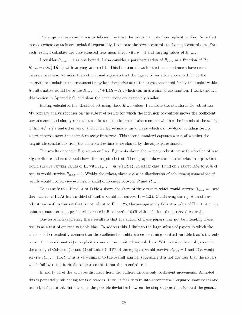
Having calculated the identified set using these Rmax values, I consider two standards for robustness.

My primary analysis focuses on the subset of results for which the inclusion of controls moves the coefficient

towards zero, and simply asks whether the set includes zero. I also consider whether the bounds of the set fall

within +/- 2.8 standard errors of the controlled estimate, an analysis which can be done including results

where controls move the coefficient away from zero. This second standard captures a test of whether the

magnitude conclusions from the controlled estimate are shared by the adjusted estimate.

The results appear in Figures 4a and 4b. Figure 4a shows the primary robustness with rejection of zero;

Figure 4b uses all results and shows the magnitude test. These graphs show the share of relationships which

would survive varying values of Π, with Rmax = min{ΠR, 1}. In either case, I find only about 15% to 20% of

results would survive Rmax = 1. Within the others, there is a wide distribution of robustness; some share of

results would not survive even quite small differences between R and Rmax.

To quantify this, Panel A of Table 4 shows the share of these results which would survive Rmax = 1 and

three values of Π. At least a third of studies would not survive Π = 1.25. Considering the rejection-of-zero

robustness, within this set that is not robust to Π = 1.25, the average study fails at a value of Π = 1.14 or, in

point estimate terms, a predicted increase in R-squared of 0.05 with inclusion of unobserved controls.

One issue in interpreting these results is that the author of these papers may not be intending these

results as a test of omitted variable bias. To address this, I limit to the large subset of papers in which the

authors either explicitly comment on the coefficient stability (since remaining omitted variable bias is the only

reason that would matter) or explicitly comment on omitted variable bias. Within this subsample, consider

the analog of Columns (1) and (3) of Table 4: 21% of these papers would survive Rmax = 1 and 41% would

survive Rmax = 1.5R. This is very similar to the overall sample, suggesting it is not the case that the papers

which fail by this criteria do so because this is not the intended test.

In nearly all of the analyses discussed here, the authors discuss only coefficient movements. As noted,

this is potentially misleading for two reasons. First, it fails to take into account the R-squared movements and,

second, it fails to take into account the possible deviation between the simple approximation and the general

26

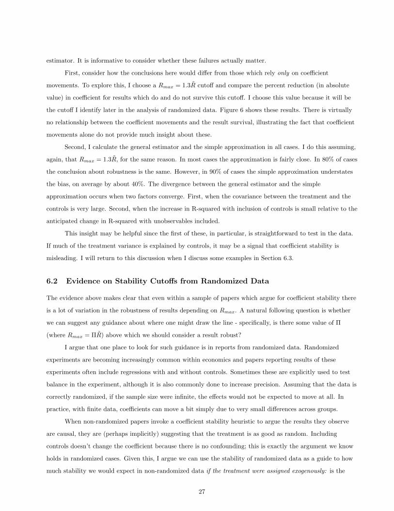
estimator. It is informative to consider whether these failures actually matter.

First, consider how the conclusions here would differ from those which rely only on coefficient

movements. To explore this, I choose a Rmax = 1.3R cutoff and compare the percent reduction (in absolute

value) in coefficient for results which do and do not survive this cutoff. I choose this value because it will be

the cutoff I identify later in the analysis of randomized data. Figure 6 shows these results. There is virtually

no relationship between the coefficient movements and the result survival, illustrating the fact that coefficient

movements alone do not provide much insight about these.

Second, I calculate the general estimator and the simple approximation in all cases. I do this assuming,

again, that Rmax = 1.3R, for the same reason. In most cases the approximation is fairly close. In 80% of cases

the conclusion about robustness is the same. However, in 90% of cases the simple approximation understates

the bias, on average by about 40%. The divergence between the general estimator and the simple

approximation occurs when two factors converge. First, when the covariance between the treatment and the

controls is very large. Second, when the increase in R-squared with inclusion of controls is small relative to the

anticipated change in R-squared with unobservables included.

This insight may be helpful since the first of these, in particular, is straightforward to test in the data.

If much of the treatment variance is explained by controls, it may be a signal that coefficient stability is

misleading. I will return to this discussion when I discuss some examples in Section 6.3.

6.2 Evidence on Stability Cutoffs from Randomized Data

The evidence above makes clear that even within a sample of papers which argue for coefficient stability there

is a lot of variation in the robustness of results depending on Rmax. A natural following question is whether

we can suggest any guidance about where one might draw the line - specifically, is there some value of Π

(where Rmax = ΠR) above which we should consider a result robust?

I argue that one place to look for such guidance is in reports from randomized data. Randomized

experiments are becoming increasingly common within economics and papers reporting results of these

experiments often include regressions with and without controls. Sometimes these are explicitly used to test

balance in the experiment, although it is also commonly done to increase precision. Assuming that the data is

correctly randomized, if the sample size were infinite, the effects would not be expected to move at all. In

practice, with finite data, coefficients can move a bit simply due to very small differences across groups.

When non-randomized papers invoke a coefficient stability heuristic to argue the results they observe

are causal, they are (perhaps implicitly) suggesting that the treatment is as good as random. Including

controls doesn’t change the coefficient because there is no confounding; this is exactly the argument we know

holds in randomized cases. Given this, I argue we can use the stability of randomized data as a guide to how

much stability we would expect in non-randomized data if the treatment were assigned exogenously: is the

27

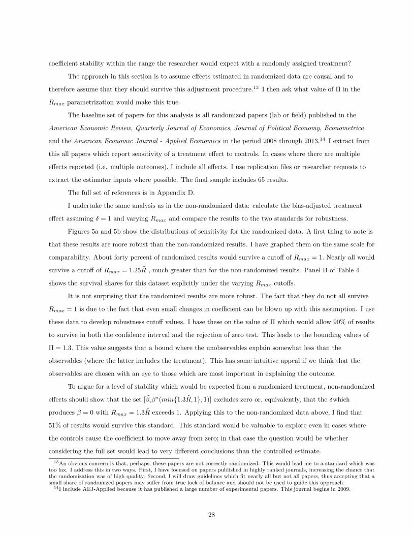
coefficient stability within the range the researcher would expect with a randomly assigned treatment?

The approach in this section is to assume effects estimated in randomized data are causal and to

therefore assume that they should survive this adjustment procedure.13 I then ask what value of Π in the

Rmax parametrization would make this true.

The baseline set of papers for this analysis is all randomized papers (lab or field) published in the

American Economic Review, Quarterly Journal of Economics, Journal of Political Economy, Econometrica

and the American Economic Journal - Applied Economics in the period 2008 through 2013.14 I extract from

this all papers which report sensitivity of a treatment effect to controls. In cases where there are multiple

effects reported (i.e. multiple outcomes), I include all effects. I use replication files or researcher requests to

extract the estimator inputs where possible. The final sample includes 65 results.

The full set of references is in Appendix D.

I undertake the same analysis as in the non-randomized data: calculate the bias-adjusted treatment

effect assuming δ = 1 and varying Rmax and compare the results to the two standards for robustness.

Figures 5a and 5b show the distributions of sensitivity for the randomized data. A first thing to note is

that these results are more robust than the non-randomized results. I have graphed them on the same scale for

comparability. About forty percent of randomized results would survive a cutoff of Rmax = 1. Nearly all would

survive a cutoff of Rmax = 1.25R , much greater than for the non-randomized results. Panel B of Table 4

shows the survival shares for this dataset explicitly under the varying Rmax cutoffs.

It is not surprising that the randomized results are more robust. The fact that they do not all survive

Rmax = 1 is due to the fact that even small changes in coefficient can be blown up with this assumption. I use

these data to develop robustness cutoff values. I base these on the value of Π which would allow 90% of results

to survive in both the confidence interval and the rejection of zero test. This leads to the bounding values of

Π = 1.3. This value suggests that a bound where the unobservables explain somewhat less than the

observables (where the latter includes the treatment). This has some intuitive appeal if we think that the

observables are chosen with an eye to those which are most important in explaining the outcome.

To argue for a level of stability which would be expected from a randomized treatment, non-randomized

effects should show that the set [β,β∗(min{1.3R, 1}, 1)] excludes zero or, equivalently, that the δwhich

produces β = 0 with Rmax = 1.3R exceeds 1. Applying this to the non-randomized data above, I find that

51% of results would survive this standard. This standard would be valuable to explore even in cases where

the controls cause the coefficient to move away from zero; in that case the question would be whether

considering the full set would lead to very different conclusions than the controlled estimate.

13An obvious concern is that, perhaps, these papers are not correctly randomized. This would lead me to a standard which wastoo lax. I address this in two ways. First, I have focused on papers published in highly ranked journals, increasing the chance thatthe randomization was of high quality. Second, I will draw guidelines which fit nearly all but not all papers, thus accepting that asmall share of randomized papers may suffer from true lack of balance and should not be used to guide this approach.

14I include AEJ-Applied because it has published a large number of experimental papers. This journal begins in 2009.

28

6.3 Examples

Before concluding it is informative to consider some examples of when performing this adjustment would

impact conclusions. In the first example below I compare several results with similar coefficient movements

but very different R-squared movements. In the second I discuss a case in which the simple approximation is

far from the general estimator. In all cases I consider these examples using δ = 1 and the bounding value for

Rmax developed based on the randomized data described above.

Importance of R-Squared Movements

To illustrate the dual role of coefficient stability and R-squared movements, I identify three results from the

set of papers above which have similar percent coefficient movements with inclusion of controls but vary in

their R-squared changes. The three cases are chosen not for their topical similarity but simply for the similar

coefficient changes.

The first result is drawn from Lavy (2009), who consider the impact of teacher performance pay on test

scores. The result used is the effect on average math scores. The second result is drawn from Brunnermeier

and Nagel (2008), who consider whether wealth fluctuations generate changes in portfolio allocations. The

result used is the relationship between the change in financial wealth and the share of wealth invested in risky

assets. The third result is drawn from Olken and Barron (2009) who explore the relationship between

checkpoints on Indonesian roads and bribes paid. The result used is the relationship between the total

payments and number of checkpoints.

Table 5 shows in the first columns the coefficient and R-squared values with and without controls. I

then report the percentage change in coefficients when controls are added. The three cases all have quite

stable coefficients, with coefficient changes in the range of 3% to 5.5%. The final column shows the

bias-adjusted β under the proportional selection assumption with δ = 1 and Rmax = 1.3R. The cases differ

significantly in the impact of this adjustment on their conclusions. For both Lavy (2009) and Olken and

Barron (2009) the bias adjustment makes a fairly small difference. However, for the Brunnermeier and Nagel

(2008) result the difference in coefficients is very large.

This distinction arises due to the varying movements in R-squared values across the three cases. The

two cases with small bias adjustments are those where the percentage change in R-squared with inclusion of

controls is very big.

Simple Approximation Error

In many cases the simple approximation is close to the general estimator and taking into account both

coefficient movements and R-squared movements in a simple way will provide a good bias estimate. However,

29

this is not always the case and it is informative to consider an example where these deviate significantly and

the simple adjustment would be misleading.

Nunn and Wantchekon (2011) analyze the impact of the slave trade on mistrust in Africa. This is a

salient example because the authors worry explicitly about unobserved differences across areas, and present a

number of arguments to support the interpretation of their results as causal. In contrast to most papers in this

literature, they undertake direct calculations based on the theory in Altonji, Elder and Taber (2005). They use

coefficient movements in their regressions to calculate the value of δ which would be required to produce

β = 0. They argue the results are robust because all the calculated values of δ are greater than 1. Equivalently,

the adjusted treatment effects have the same sign as their controlled effects if δ = 1.

Although it is not made explicit, the calculations they undertake in the paper implicitly assume that

Rmax = R+ (R− R).15 In words, they assumes the unobservables explain as much of the outcome as the

observables (ignoring that the treatment is part of the observables). In practice, the R-squared values in their

regressions do not move much; as an example, in the first row of their Table 4, considering the “Trust

Relatives” measure, adding controls increases R-squared from 0.115 to 0.133. Their adjustment assumes that

the fully controlled R-squared would be 0.151. The cutoff generated based on the randomized data above

would suggest a value of 0.173.

A set of results from their Table 4 are reported in Table 6. The first columns show their estimated

effects, and the third column generates the simple approximation to β using their implicit assumption on

Rmax and δ = 1. As stated in their paper, the effects here are of very similar magnitude to the main controlled

effects. The fourth column shows the simple approximation of β using the assumption that Rmax = 1.3R and

δ = 1. The adjutsmetns are larger here, but the conclusions are quite similar.

The final column shows the β estimated using the full estimator rather than the approximation (along

with the assumptions that Rmax = 1.3R and δ = 1). The results are very different. In four of five cases the

bias-adjusted β is of a different sign than their controlled effects and typically quite large in magnitude. It is

worth noting that even if I adopt their conservative assumption on Rmax two of the five results would show

bias-adjusted values above zero (results available from the author).

In looking at the raw data it is clear why this is the case. The controls used explain a large share of the

variation in the treatment. This suggests a high covariance between treatment and controls which, in

combination with the relatively small R-squared movements, generates a large error in the simple

approximation.

15They draw this from Bellows and Miguel (2009).

30

7 Conclusion

This paper develops a formal language for discussing robustness of treatment effects, related to the popular

heuristic of exploring coefficient sensitivity to controls. I connect this heuristic to the assumption of

proportional selection on observed and unobserved variables. I describe an implementation strategy for

generating bounds on treatment effects and show validation in two empirical contexts. Applying this to the

economics literature, and drawing guidelines for expected coefficient sensitivity from randomized results, I

develop a full bounding argument.

I suggest a standard for robustness relying on this estimator which could be easily implemented by

researchers. A key issue is the need to make an assumption about the share of the outcome variance would

could be explained by observed and unobserved variables together. I suggest a standard based on the

performance of this estimator in randomized data. It may be possible to develop a better intuition about this

in a given context.

The core insight here is to recognize that coefficient stability on its own is at best uninformative and at

worst very misleading. It must be combined with information about R-squared movements to develop an

argument. In addition, in the common empirical case in which the researcher is including multiple observed

controls, it is possible to observe very stable coefficients and sizable R-squared movements even in the presence

of large bias. This strongly argues for approaching these robustness arguments formally.

31

References

Almond, Douglas and Bhashkar Mazumder, “Health Capital and the Prenatal Environment:The Effect of Ramadan Observance during Pregnancy,” American Economic Journal: AppliedEconomics, October 2011, 3 (4), 56–85.

and Janet Currie, “Killing Me Softly: The Fetal Origins Hypothesis,” Journal of EconomicPerspectives, Summer 2011, 25 (3), 153–72.

Altonji, Joeseph, Timothy Conley, Todd Elder, and Christopher Taber, “Methods forUsing Selection on Observed Variables to Address Selection on Unobserved Variables,” 2011.Mimeo, Yale University.

Altonji, Joseph G., Todd Elder, and Christopher R. Taber, “Using Selection on ObservedVariables to Assess Bias from Unobservables When Evaluating Swan-Ganz Catheterization,”American Economic Review, 2008, 98 (2), 345–50.

Angrist, Joshua D. and Jorn-Steffen Pischke, “The Credibility Revolution in EmpiricalEconomics: How Better Research Design Is Taking the Con out of Econometrics,” Journal ofEconomic Perspectives, Spring 2010, 24 (2), 3–30.

Chiappori, Pierre-Andrei, Sonia Oreffice, and Climent Quintana-Domeque, “FatterAttraction: Anthropometric and Socioeconomic Matching on the Marriage Market,” Journalof Political Economy, 2012, 120 (4), 659 – 695.

de Kieviet, J. F., L. Zoetebier, R. M. van Elburg, R. J. Vermeulen, and J. Oosterlaan,“Brain development of very preterm and very low-birthweight children in childhood andadolescence: a meta-analysis,” Dev Med Child Neurol, Apr 2012, 54 (4), 313–323.

Dehejia, Rajev and Sadek Wahba, “Causal Effects in Nonexperimental Studies: Reevaluatingthe Evaluation of Training Programs,” Journal of the American Statistical Association, 1999,94 (448), 1053–1062.

Falgreen-Eriksen, H. L., E. L. Mortensen, T. Kilburn, M. Underbjerg, J. Bertrand,H. Stavring, T. Wimberley, J. Grove, and U. S. Kesmodel, “The effects of low tomoderate prenatal alcohol exposure in early pregnancy on IQ in 5-year-old children,” BJOG,Sep 2012, 119 (10), 1191–1200.

Heckman, James and Joseph Hotz, “Choosing Among Alternative Nonexperimental Methodsfor Estimating the Impact of Social Programs: The Case of Manpower Training,” Journal ofthe American Statistical Association, 1989, 84 (408), 862–874.

Henderson, J., R. Gray, and P. Brocklehurst, “Systematic review of effects of low-moderateprenatal alcohol exposure on pregnancy outcome,” BJOG, Mar 2007, 114 (3), 243–252.

Imbens, Guido, “Sensitivity to Exogeneity Assumptions in Program Evaluation,” AmericanEconomic Review, 2003, 93 (2), 126–132.

Kramer, M. S., F. Aboud, E. Mironova et al., “Breastfeeding and child cognitivedevelopment: new evidence from a large randomized trial,” Arch. Gen. Psychiatry, May 2008,65 (5), 578–584.

Lacetera, Nicola, Devin G. Pope, and Justin R. Sydnor, “Heuristic Thinking and LimitedAttention in the Car Market,” American Economic Review, August 2012, 102 (5), 2206–36.

LaLonde, Robert J, “Evaluating the Econometric Evaluations of Training Programs withExperimental Data,” American Economic Review, September 1986, 76 (4), 604–20.

Lumley, J., C. Chamberlain, T. Dowswell, S. Oliver, L. Oakley, and L. Watson,“Interventions for promoting smoking cessation during pregnancy,” Cochrane Database SystRev, 2009, (3), CD001055.

32

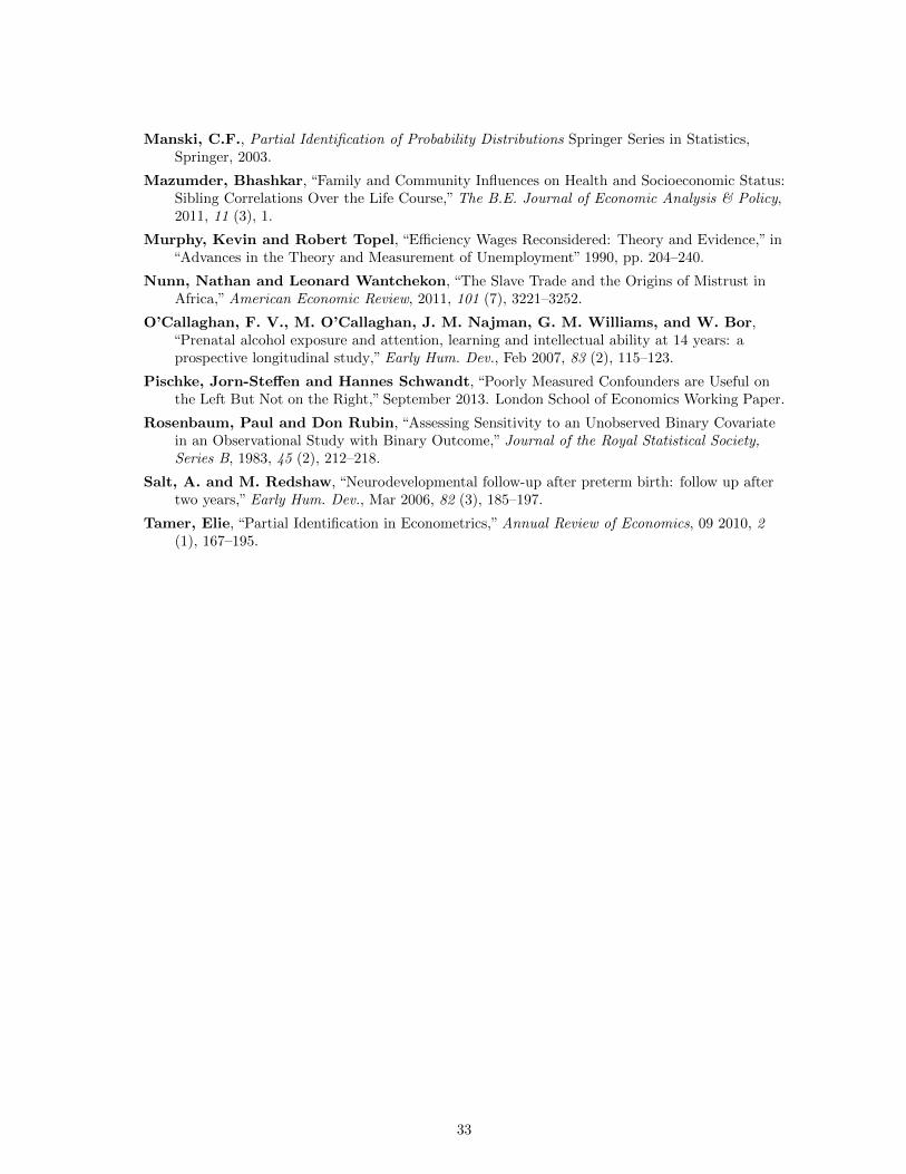
Manski, C.F., Partial Identification of Probability Distributions Springer Series in Statistics,Springer, 2003.

Mazumder, Bhashkar, “Family and Community Influences on Health and Socioeconomic Status:Sibling Correlations Over the Life Course,” The B.E. Journal of Economic Analysis & Policy,2011, 11 (3), 1.

Murphy, Kevin and Robert Topel, “Efficiency Wages Reconsidered: Theory and Evidence,” in“Advances in the Theory and Measurement of Unemployment” 1990, pp. 204–240.

Nunn, Nathan and Leonard Wantchekon, “The Slave Trade and the Origins of Mistrust inAfrica,” American Economic Review, 2011, 101 (7), 3221–3252.

O’Callaghan, F. V., M. O’Callaghan, J. M. Najman, G. M. Williams, and W. Bor,“Prenatal alcohol exposure and attention, learning and intellectual ability at 14 years: aprospective longitudinal study,” Early Hum. Dev., Feb 2007, 83 (2), 115–123.

Pischke, Jorn-Steffen and Hannes Schwandt, “Poorly Measured Confounders are Useful onthe Left But Not on the Right,” September 2013. London School of Economics Working Paper.

Rosenbaum, Paul and Don Rubin, “Assessing Sensitivity to an Unobserved Binary Covariatein an Observational Study with Binary Outcome,” Journal of the Royal Statistical Society,Series B, 1983, 45 (2), 212–218.

Salt, A. and M. Redshaw, “Neurodevelopmental follow-up after preterm birth: follow up aftertwo years,” Early Hum. Dev., Mar 2006, 82 (3), 185–197.

Tamer, Elie, “Partial Identification in Econometrics,” Annual Review of Economics, 09 2010, 2(1), 167–195.

33

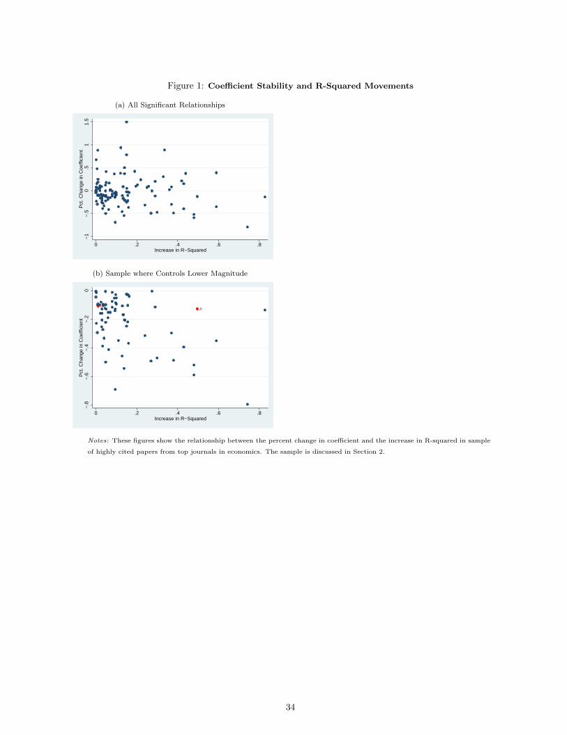
Figure 1: Coefficient Stability and R-Squared Movements

(a) All Significant Relationships

−1

−.5

0.5

11.

5P

ct. C

hang

e in

Coe

ffici

ent

0 .2 .4 .6 .8Increase in R−Squared

(b) Sample where Controls Lower Magnitude

AB

−.8

−.6

−.4

−.2

0P

ct. C

hang

e in

Coe

ffici

ent

0 .2 .4 .6 .8Increase in R−Squared

Notes: These figures show the relationship between the percent change in coefficient and the increase in R-squared in sample

of highly cited papers from top journals in economics. The sample is discussed in Section 2.

34

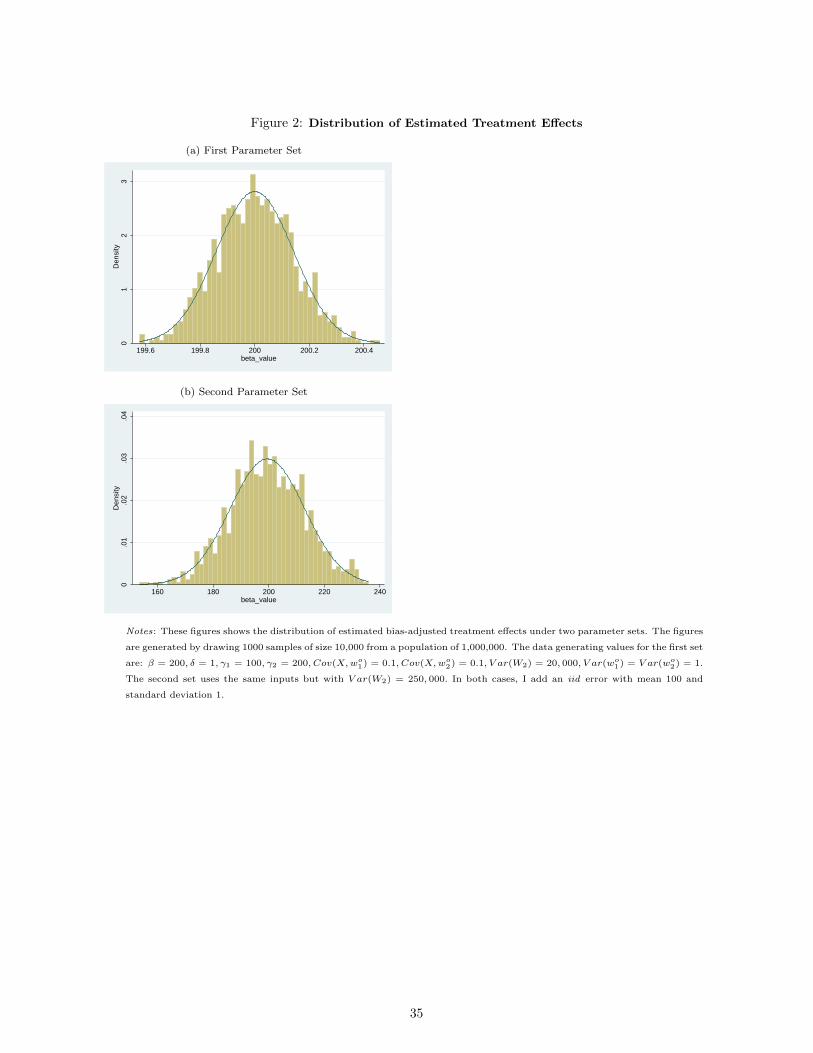
Figure 2: Distribution of Estimated Treatment Effects

(a) First Parameter Set

01

23

Den

sity

199.6 199.8 200 200.2 200.4beta_value

(b) Second Parameter Set

0.0

1.0

2.0

3.0

4D

ensi

ty

160 180 200 220 240beta_value

Notes: These figures shows the distribution of estimated bias-adjusted treatment effects under two parameter sets. The figures

are generated by drawing 1000 samples of size 10,000 from a population of 1,000,000. The data generating values for the first set

are: β = 200, δ = 1, γ1 = 100, γ2 = 200, Cov(X,wo1) = 0.1, Cov(X,wo2) = 0.1, V ar(W2) = 20, 000, V ar(wo1) = V ar(wo2) = 1.

The second set uses the same inputs but with V ar(W2) = 250, 000. In both cases, I add an iid error with mean 100 and

standard deviation 1.

35

Figure 3: NLSY Wage Data Simulation

(a) “True”, Controlled and Adjusted Beta

010

020

030

040

0A

djus

ted

Den

sity

050

100

150

Tru

e, C

ontr

olle

d E

ffect

Den

sity

.07 .08 .09 .1 .11Estimate

True Treatment Effect Controlled BetaAdjusted Beta

(b) Distribution of Estimated Delta

0.5

11.

5

−1 0 1 2 3Calculated Delta

(c) “True”, Controlled and Simple Approximation AdjustedBeta

010

020

030

040

0A

djus

ted

Den

sity

050

100

150

Tru

e, C

ontr

olle

d E

ffect

Den

sity

.07 .08 .09 .1 .11Estimate

True Treatment Effect Controlled BetaAdjusted Beta, Simple Estimator

Notes: These figures show results from the validation using the constructed NLSY wage dataset. The analysis is described in

Section 5.

36

Figure 4: Robustness of Stability Results in Economics Literature

(a) Rejection of Zero, Rmax = ΠR.

Survive Rmax=1: 0.195

.3.4

.5.6

.7.8

.91

Sha

re o

f Res

ults

With

sig

n(β)

=si

gn(β

tilde

)

1 2 3 4 5 6 7 8 9 10Multiplier Π : Rmax = Π *Rtilde

(b) Results within +/- 2.8 SE, Rmax = ΠR.

Survive Rmax=1: 0.135

.3.4

.5.6

.7.8

.91

Sha

re o

f Res

ults

with

β +

/− 1

.64

SE

from

β til

de

1 2 3 4 5 6 7 8 9 10Multiplier Π : Rmax = Π *Rtilde

Notes: These graphs show the performance of non-randomized results under the proportional selection adjustment. Each

figure graphs the share of results which would survive varying parametrizations of Rmax, in all cases assuming δ = 1. Sub-

Figure a indicates the share of results which would survive Rmax = ΠR for varying values of Π, with the survival in this case

meaning the identified set does not include zero. This figure contains only relationships where the effect is significant with

controls and adding the controls moves the coefficient toward zero. Sub-Figure b indicates the share of results for which the

full identified set would be within 2.8 standard errors of the controlled coefficient. This sub-figure includes all relationships.

37

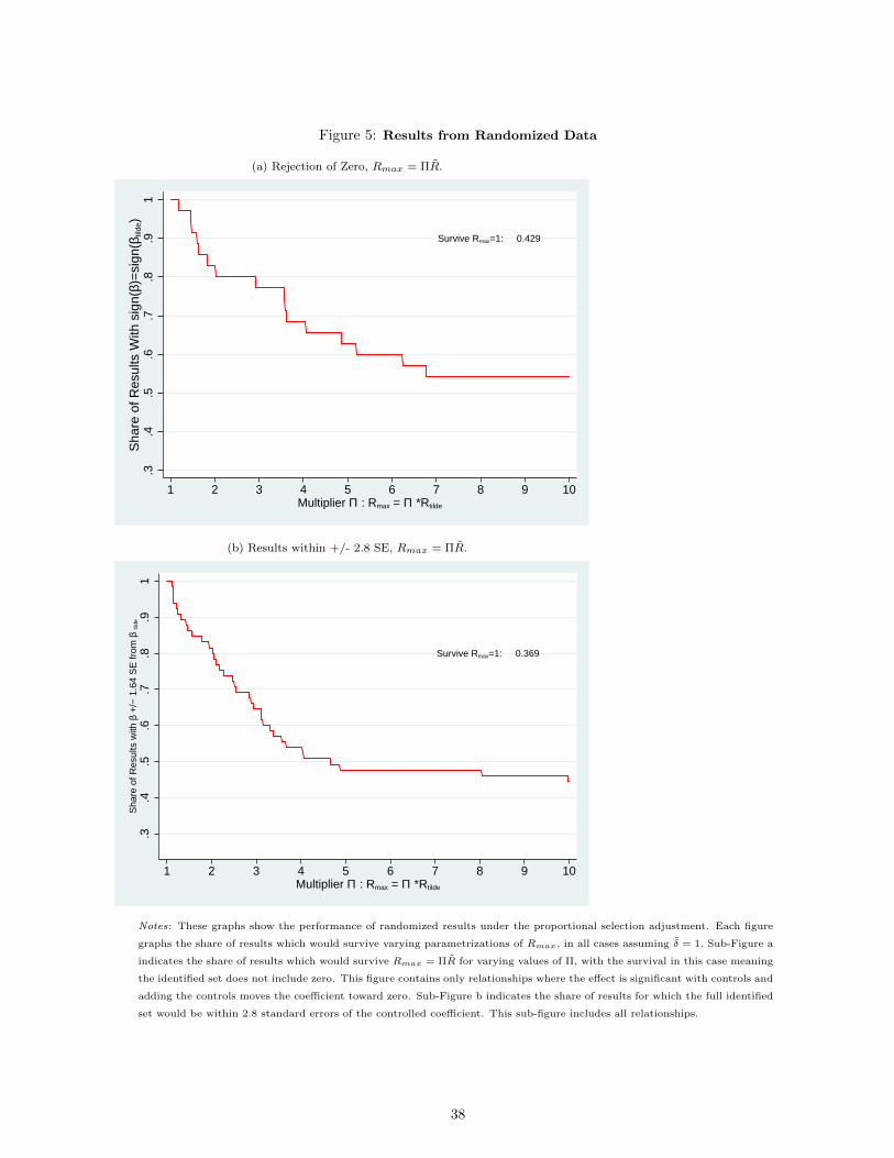
Figure 5: Results from Randomized Data

(a) Rejection of Zero, Rmax = ΠR.

Survive Rmax=1: 0.429

.3.4

.5.6

.7.8

.91

Sha

re o

f Res

ults

With

sig

n(β)

=si

gn(β

tilde

)

1 2 3 4 5 6 7 8 9 10Multiplier Π : Rmax = Π *Rtilde

(b) Results within +/- 2.8 SE, Rmax = ΠR.

Survive Rmax=1: 0.369

.3.4

.5.6

.7.8

.91

Sha

re o

f Res

ults

with

β +

/− 1

.64

SE

from

β til

de

1 2 3 4 5 6 7 8 9 10Multiplier Π : Rmax = Π *Rtilde

Notes: These graphs show the performance of randomized results under the proportional selection adjustment. Each figure

graphs the share of results which would survive varying parametrizations of Rmax, in all cases assuming δ = 1. Sub-Figure a

indicates the share of results which would survive Rmax = ΠR for varying values of Π, with the survival in this case meaning

the identified set does not include zero. This figure contains only relationships where the effect is significant with controls and

adding the controls moves the coefficient toward zero. Sub-Figure b indicates the share of results for which the full identified

set would be within 2.8 standard errors of the controlled coefficient. This sub-figure includes all relationships.

38

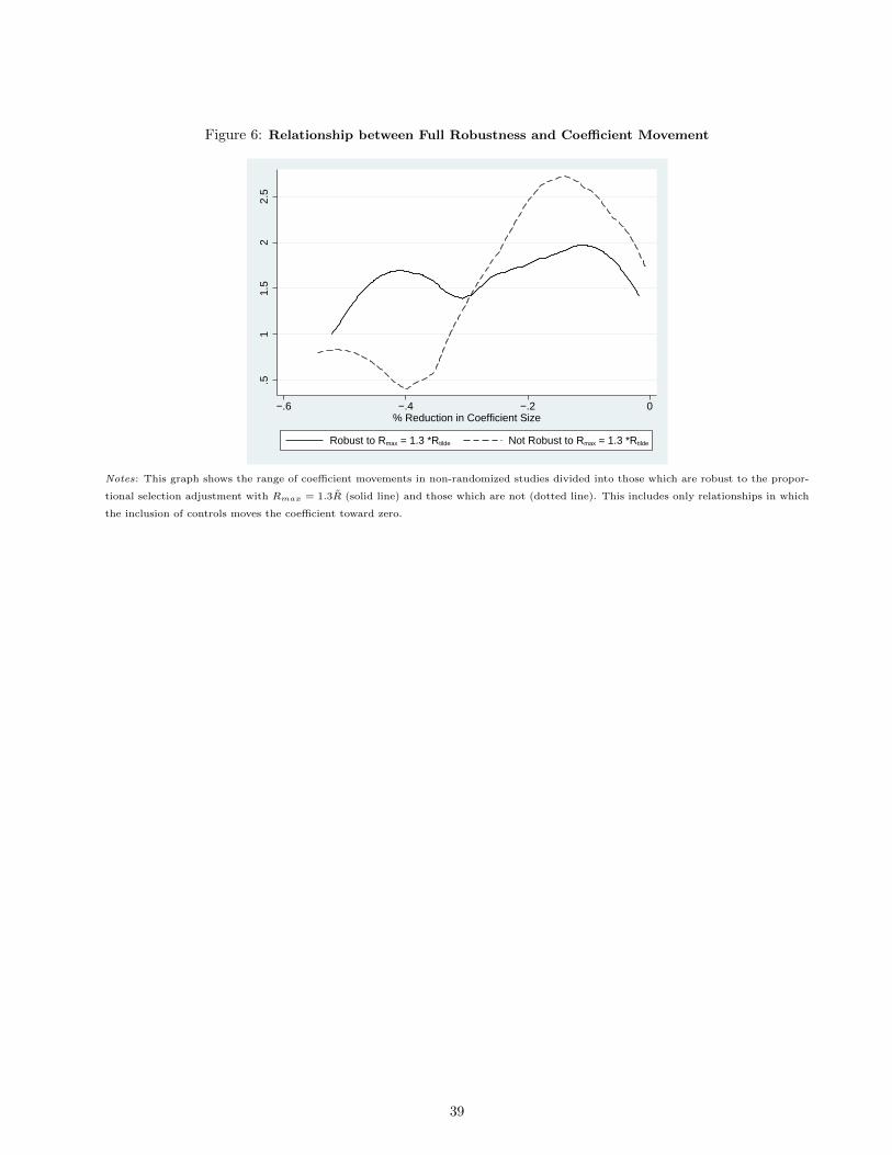
Figure 6: Relationship between Full Robustness and Coefficient Movement

.51

1.5

22.

5

−.6 −.4 −.2 0% Reduction in Coefficient Size

Robust to Rmax = 1.3 *Rtilde Not Robust to Rmax = 1.3 *Rtilde

Notes: This graph shows the range of coefficient movements in non-randomized studies divided into those which are robust to the propor-

tional selection adjustment with Rmax = 1.3R (solid line) and those which are not (dotted line). This includes only relationships in which

the inclusion of controls moves the coefficient toward zero.

39

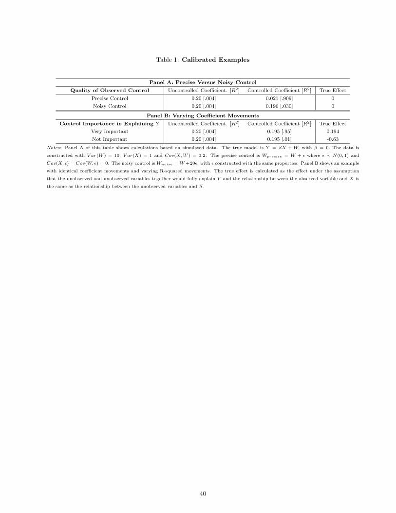
Table 1: Calibrated Examples

Panel A: Precise Versus Noisy Control

Quality of Observed Control Uncontrolled Coefficient. [R2] Controlled Coefficient [R2] True Effect

Precise Control 0.20 [.004] 0.021 [.909] 0

Noisy Control 0.20 [.004] 0.196 [.030] 0

Panel B: Varying Coefficient Movements

Control Importance in Explaining Y Uncontrolled Coefficient. [R2] Controlled Coefficient [R2] True Effect

Very Important 0.20 [.004] 0.195 [.95] 0.194

Not Important 0.20 [.004] 0.195 [.01] -0.63

Notes: Panel A of this table shows calculations based on simulated data. The true model is Y = βX + W, with β = 0. The data is

constructed with V ar(W ) = 10, V ar(X) = 1 and Cov(X,W ) = 0.2. The precise control is Wprecise = W + ε where ε ∼ N(0, 1) and

Cov(X, ε) = Cov(W, ε) = 0. The noisy control is Wnoise = W+20ε, with ε constructed with the same properties. Panel B shows an example

with identical coefficient movements and varying R-squared movements. The true effect is calculated as the effect under the assumption

that the unobserved and unobserved variables together would fully explain Y and the relationship between the observed variable and X is

the same as the relationship between the unobserved variables and X.

40

41

Table

2:

Sim

ula

ted

Data

(1)

(2)

(3)

(4)

(5)

(6)

Ass

um

pti

on

s:

β=

200

β=

200

β=

200

β=

200

β=

200

β=

200

γ1

=100

γ1

=100

γ1

=−

100

γ1

=100

γ1

=−

100

γ1

=−

100

γ2

=200

γ2

=200

γ2

=200

γ2

=200

γ2

=200

γ2

=200

Cov(X,wo 1)

=0.0

5Cov(X,wo 1)

=0.1

Cov(X,wo 1)

=−

0.1

Cov(X,wo 1)

=0.1

Cov(X,wo 1)

=−

0.1

Cov(X,wo 1)

=−

0.0

1

Cov(X,wo 2)

=0.1

Cov(X,wo 2)

=0.1

Cov(X,wo 2)

=−

0.3

5Cov(X,wo 2)

=0.1

Cov(X,wo 2)

=−

0.3

5Cov(X,wo 2)

=−

0.0

35

Var(W

2)

=200

Var(W

2)

=200

Var(W

2)

=200

Var(W

2)

=250,000

Var(W

2)

=250,000

Var(W

2)

=250,000

β[R

]225.1

[0.5

0]

230.1

[0.5

1]

139.7

[0.3

0]

380.0

[0.3

5]

-160.0

[0.1

3]

164.0

[0.0

8]

β[R

]200.1

[0.9

9]

200.1

[0.9

9]

199.7

[0.9

9]

353.1

[0.4

4]

-145.8

2[0

.25]

169.9

[0.2

4]

Genera

lE

stim

ato

rβ

β∗

=200

β∗

=200

β∗

=200

β∗

=200

β∗

=200

β∗

=200

[Alt

ern

ati

ve

Roots

][2

200]

[1866.6

][−

633.3

][1

866.6

][−

633.3

][−

8133.3

Sim

ple

Est

imato

rβ

β∗

=200

β∗

=200.0

0025

β∗

=199.9

8β∗

=202.2

6β∗

=−

59.9

β=

199.8

9

Note

s:

This

table

use

sth

evari

ous

est

imato

rspro

pose

din

Monte

Carl

osi

mula

tions.

Resu

lts

rep

ort

the

asy

mpto

tic

valu

eof

the

est

imate

s.A

llsi

mula

tions

ass

um

eδ=

1,Rmax

=1

and

the

vari

ance

ofwo 1

andwo 2

are

both

equal

to1.

*For

the

sim

ula

tion

incolu

mn

(5)

inP

anel

Cth

evari

ance

ofW

2is

set

at

250,0

00

because

itw

as

oth

erw

ise

imp

oss

ible

togenera

tedata

wit

h

this

covari

ance

stru

ctu

re.

42

Tab

le3:

Mate

rnal

Behavio

r,C

hild

IQand

Bir

thW

eig

ht

(1)

(2)

(3)

(4)

(5)

(6)

(7)

PanelA:Child

IQ,Standardized

(N

LSY)(Rmax

=.6

1)

Tre

atm

en

tV

aria

ble

Base

lin

eE

ffec

tC

on

troll

edE

ffec

tN

ull

Reje

ct?

Sib

lin

gF

EId

en

tifi

edδ

forβ

=0

Iden

tifi

edS

et(S

td.

Err

or)

,[R

2]

(Std

.E

rror),

[R2]

(extr

nl.

evid

.)E

stim

ate

Set

Giv

enRmax

(Sim

ple

Appro

x.)

Bre

ast

feed

(Month

s)0.0

45∗∗∗

(.003)

[.045]

0.0

17∗∗∗(.

002)

[.256]

No

-0.0

07

(.005)

[-0.0

33,0

.017]

0.3

7[-

0.0

28,0

.017]

Dri

nk

inP

reg.

(Any)

0.1

76∗∗∗(.

026)

[.008]

0.0

50∗∗(.

023)

[.249]

No

0.0

26

(.036)

[-0.1

46,0

.050]

0.2

6[-

0.1

38,0

.050]

LB

W+

Pre

term

-0.1

88∗∗∗(.

057)

[.004]

-0.1

25∗∗∗(.

050)

[.251]

Yes

-0.1

11

(.070)

[-0.1

24,-

0.0

33]†

1.3

7[-

0.1

24,-

0.0

33]†

PanelB:Birth

Weig

htin

Gram

s(N

LSY)(Rmax

=.5

3)

Tre

atm

en

tV

aria

ble

Base

lin

eE

ffec

tC

on

troll

edE

ffec

tN

ull

Reje

ct?

Sib

lin

gF

EId

en

tifi

edδ

forβ

=0

Iden

tifi

edS

et(S

td.

Err

or)

,[R

2]

(Std

.E

rror),

[R2]

(extr

nl.

evid

.)E

stim

ate

Set

Giv

enRmax

(Sim

ple

Appro

x.)

Sm

okin

gin

Pre

g-1

83.1∗∗∗

(12.9

)[.31]

-172.5∗∗∗(1

3.3

)[.35]

Yes

-94.3∗∗∗(2

7.6

)[-

172.5

,-30.3

]†1.0

8[-

172.5

,-115.7

]†

Dri

nk

inP

reg.

(Am

t)-1

6.7∗∗∗(5

.15)

[.30]

-14.1∗∗∗

(5.0

6)

[.34]

No

-1.5

3(7

.48)

[-14.1

,0.4

9]

0.9

6[-

14.1

,-1.0

5]†

Note

s:

This

table

show

sth

evalidati

on

resu

lts

for

the

analy

sis

of

the

impact

of

mate

rnal

behavio

ron

child

bir

thw

eig

ht

and

IQ.

Base

line

eff

ects

inclu

de

only

contr

ols

for

child

sex

and

(1)

age

dum

mie

sin

the

case

of

IQand

(2)

gest

ati

on

week

inth

ecase

of

bir

thw

eig

ht.

Full

contr

ols

:ra

ce,

age,

educati

on,

incom

e,

mari

tal

statu

s.Sib

ling

fixed

eff

ects

est

imate

scom

efr

om

NL

SY

inall

panels

.T

he

identi

fied

set

inC

olu

mn

(5)

isb

ounded

belo

wbyβ

and

ab

ove

byβ∗

calc

ula

ted

base

donRmax

giv

en

inth

eto

pro

wof

each

panel

andδ

=1.†

identi

fied

set

exclu

des

zero

.T

heRmax

calc

ula

tion

inC

olu

mn

(6)

isdone

under

the

ass

um

pti

on

thatδ

=1∗

signifi

cant

at

10%

level,∗∗

signifi

cant

at

5%

level,∗∗∗

signifi

cant

at

1%

level.

43

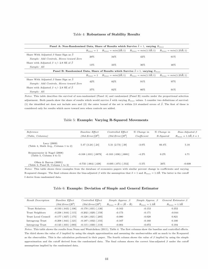
Table 4: Robustness of Stability Results

Panel A: Non-Randomized Data, Share of Results which Survive δ = 1, varying Rmax

Rmax = 1 Rmax = min(2R; 1) Rmax = min(1.5R; 1) Rmax = min(1.25R; 1)

Share With Adjusted β Same Sign as β20% 34% 42% 61%

Sample: Add Controls, Moves toward Zero

Share with Adjusted β +/- 2.8 SE of β13% 33% 36% 46%

Sample: All

Panel B: Randomized Data, Share of Results which Survive δ = 1, varying Rmax

Rmax = 1 Rmax = min(2R; 1) Rmax = min(1.5R; 1) Rmax = min(1.25R; 1)

Share With Adjusted β Same Sign as β42% 82% 91% 97%

Sample: Add Controls, Moves toward Zero

Share with Adjusted β +/- 2.8 SE of β37% 82% 86% 91%

Sample: All

Notes: This table describes the survival of non-randomized (Panel A) and randomized (Panel B) results under the proportional selection

adjustment. Both panels show the share of results which would survive δ with varying Rmax values. I consider two definitions of survival:

(1) the identified set does not include zero and (2) the outer bound of the set is within 2.8 standard errors of β. The first of these is

considered only for results which move toward zero when controls are added.

Table 5: Example: Varying R-Squared Movements

Reference Baseline Effect Controlled Effect % Change in % Change in Bias-Adjusted β

(Table, Columns) (Std.Error)[R2] (Std.Error)[R2] Coefficient R-Squared Rmax = 1.3R, δ = 1

Lavy (2009)(Table 4, Math Avg., Column 1 to 2)

5.47 (3.24) [.24] 5.31 (2.73) [.39] -3.0% 66.4% 5.18

Brunnermeier & Nagel (2008)(Table 5, Column 4 to 5)

-0.108 (.031) [.0879] -0.103 (.036) [.0881] -4.2% 0.2% 4.71

Olken & Barron (2009))(Table 2, Panel B, Column 1 to 2)

-0.735 (.064) [.438] -0.695 (.071) [.552] -5.5% 26% -0.608

Notes: This table shows three examples from the database of economics papers with similar percent change in coefficients and varying

R-squared changes. The final column shows the bias-adjusted β with the assumption that δ = 1 and Rmax = 1.3R. The latter is the cutoff

I derive from randomized data.

Table 6: Example: Deviation of Simple and General Estimator

Result Description Baseline Effect Controlled Effect Simple Approx. β Simple Approx. β General Estimator β

(Std.Error)[R2] (Std.Error)[R2] Rmax = R + (R− R) Rmax = 1.3R Rmax = 1.3R

Trust Relatives -0.193 (.043) [.106] -0.178 (.031) [.130] -0.162 -0.153 0.352

Trust Neighbors -0.238 (.044) [.115] -0.202 (.029) [.159] -0.173 -0.171 -0.044

Trust Local Council -0.177 (.027) [.175] -0.128 (.021) [.205] -0.080 -0.028 0.821

Intragroup Trust -0.208 (.041) [.121] -0.187 (.032) [.155] -0.167 -0.160 0.100

Intergroup Trust -0.145 (.031) [.093] -0.115 (.030) [.119] -0.084 -0.072 0.194

Notes: This table shows the results from Nunn and Wantchekon (2011), Table 4. The first columns show the baseline and controlled effects.

The third shows the value of β implied by using the simple approximation and assuming the unobservables add as much to the R-squared

as the observables. This is the calculation performed in their paper. The fourth column shows the value of β implied by using the simple

approximation and the cutoff derived from the randomized data. The final column shows the correct bias-adjusted β under the cutoff

assumptions implied by the randomized data.

44

Appendix for Online Publication Only

45

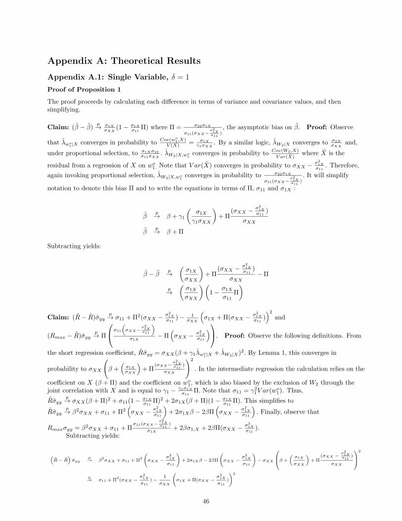
Appendix A: Theoretical Results

Appendix A.1: Single Variable, δ = 1

Proof of Proposition 1

The proof proceeds by calculating each difference in terms of variance and covariance values, and thensimplifying.

Claim: (β − β)p→ σ1X

σXX(1− σ1X

σ11Π) where Π = σ22σ1X

σ11(σXX−σ21Xσ11

), the asymptotic bias on β. Proof: Observe

that λwo1 |X converges in probability toCov(wo1 ,X)V (X) = σ1X

γ1σXX. By a similar logic, λW2|X converges to σ2X

σXXand,

under proportional selection, to σ1Xσ22

σ11σXX. λW2|X,wo1 converges in probability to Cov(W2,X)

V ar(X)where X is the

residual from a regression of X on wo1. Note that V ar(X) converges in probability to σXX − σ21X

σ11. Therefore,

again invoking proportional selection, λW2|X,wo1 converges in probability to σ22σ1X

σ11(σXX−σ21Xσ11

). It will simplify

notation to denote this bias Π and to write the equations in terms of Π, σ11 and σ1X :

βp→ β + γ1

(σ1X

γ1σXX

)+ Π

(σXX − σ21X

σ11)

σXX

βp→ β + Π

Subtracting yields:

β − β p→(σ1X

σXX

)+ Π

(σXX − σ21X

σ11)

σXX−Π

p→(σ1X

σXX

)(1− σ1X

σ11Π

)

Claim: (R− R)σyyp→ σ11 + Π2(σXX − σ2

1X

σ11)− 1

σXX

(σ1X + Π(σXX − σ2

1X

σ11))2

and

(Rmax − R)σyyp→ Π

σ11

(σXX−

σ21Xσ11

)σ1X

−Π(σXX − σ2

1X

σ11

). Proof: Observe the following definitions. From

the short regression coefficient, Rσyy = σXX(β + γ1λwo1 |X + λW2|X)2. By Lemma 1, this converges in

probability to σXX

(β +

(σ1X

σXX

)+ Π

(σXX−σ21Xσ11

)

σXX

)2

. In the intermediate regression the calculation relies on the

coefficient on X (β + Π) and the coefficient on wo1, which is also biased by the exclusion of W2 through thejoint correlation with X and is equal to γ1 − γ1σ1X

σ11Π. Note that σ11 = γ2

1V ar(wo1). Thus,

Rσyyp→ σXX(β + Π)2 + σ11(1− σ1X

σ11Π)2 + 2σ1X(β + Π)(1− σ1X

σ11Π). This simplifies to

Rσyyp→ β2σXX + σ11 + Π2

(σXX − σ2

1X

σ11

)+ 2σ1Xβ − 2βΠ

(σXX − σ2

1X

σ11

). Finally, observe that

Rmaxσyy = β2σXX + σ11 + Πσ11(σXX−

σ21Xσ11

)

σ1X+ 2βσ1,X + 2βΠ(σXX − σ2

1X

σ11).

Subtracting yields:

(R− R

)σyy

p→ β2σXX + σ11 + Π

2

(σXX −

σ21X

σ11

)+ 2σ1Xβ − 2βΠ

(σXX −

σ21X

σ11

)− σXX

β +

(σ1X

σXX

)+ Π

(σXX −σ21Xσ11

)

σXX

2

p→ σ11 + Π2(σXX −

σ21X

σ11

)−1

σXX

(σ1X + Π(σXX −

σ21X

σ11

)

)2

46

(Rmax − R)σyyp→ β

2σXX + σ11 + Π

σ11(σXX −σ21Xσ11

)

δσ1X

+ 2βσ1,X + 2βΠ(σXX −σ21X

σ11

)

−(β2σXX + σ11 + Π

2

(σXX −

σ21X

σ11

)+ 2σ1Xβ − 2βΠ

(σXX −

σ21X

σ11

))

p→ Π

σ11

(σXX −

σ21Xσ11

)σ1X

− Π

(σXX −

σ21X

σ11

)

Claim: Define β∗ = β −[β − β

]Rmax−RR−R . Then, β∗

p→ β.

Proof: The claims above define a system of three equations in three unknowns:

(β − β)p→

(σ1X

σXX

)(1− σ1X

σ11Π

)(R− R

)σyy

p→ σ11 + Π2(σXX −σ2

1X

σ11)− 1

σXX

(σ1X + Π(σXX −

σ21X

σ11)

)2

(Rmax − R)σyyp→ Π

σ11

(σXX − σ2

1X

σ11

)σ1X

−Π

(σXX −

σ21X

σ11

)The unknowns are σ11, σ1X and Π. The system is identified and the solution is Π =

[β − β

]Rmax−RR−R . This

gives the result.

Appendix A.2: General Estimator

The approach for the general estimator is virtually identical to the simple estimator case. It will be helpful toobserve that β and R are defined exactly as above, as is Rmax.These are not impacted by the way we definethe W1index since the controls are either (1) not included or (b) fully included.

Claim: (β − β)p→ σ1X

σXX−Π

(σXX−τxσXX

)where Π = δσ1Xσ22

σ11τx, the asymptotic bias on β.

Proof: As above, βp→ β + σ1X

σXX+ σ2X

σXX. Given the proportional selection assumption and the definition of Π

above, we therefore have: βp→ β + σ1X

σXX+ Π τx

σXX. And by definition β

p→ β + Π. Differencing yields:

β − β p→ σ1X

σXX−Π

(σXX − τxσXX

)Claim: (R− R)σyy

p→ σ11 + Π2τx − 1σXX

(σ1X + Πτx)2

and (Rmax − R)σyyp→ Π

(σ11τxδσ1X

−Πτx

).

Proof: By the simple definition of R we have Rσyyp→ (β + σ1X

σXX+ Π τx

σXX)2σXX . Define the variance of

element ωoi as σωoii and the covariance of element ωoi with X as σωoix . By definition, we have:

Rσyyp→ (β + Π)2 σXX +

j∑i=1

((ψi −

σωoix

σωoii

(Π)

)2

σωoii

)+ 2(β + Π)

j∑i=1

(σωoix

(ψi −

σωoix

σωoii

(Π)

))

Note the following: σ11 =∑ji=1 ψ

2i σ

ωoii , σ1X =

[∑ji=1 ψiσ

ωoix

]and τx =

[σXX −

∑ji=1

(σωoix )2

σωoii

]. This therefore

simplifies to: Rσyyp→ β2σxx + σ11 + Π2τx + 2βΠ(τx) + 2βσ1X .

Finally, Rmaxσyyp→ β2σXX + σ11 + σ22 + 2βσ1,X + 2βΠτx . Subtracting yields both results.

Completion of Proof: The above claims provide a system of three equations in three unknowns (σ11,σ1X ,

47

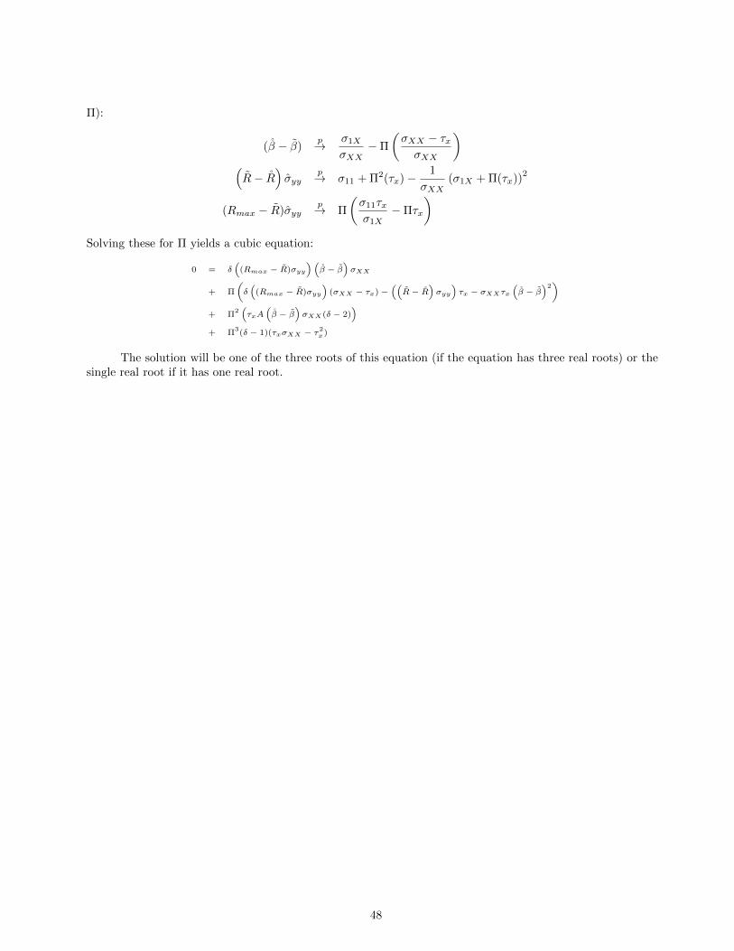
Π):

(β − β)p→ σ1X

σXX−Π

(σXX − τxσXX

)(R− R

)σyy

p→ σ11 + Π2(τx)− 1

σXX(σ1X + Π(τx))

2

(Rmax − R)σyyp→ Π

(σ11τxσ1X

−Πτx

)Solving these for Π yields a cubic equation:

0 = δ(

(Rmax − R)σyy)(

β − β)σXX

+ Π

(δ(

(Rmax − R)σyy)

(σXX − τx)−((R− R

)σyy

)τx − σXXτx

(β − β

)2)

+ Π2(τxA

(β − β

)σXX(δ − 2)

)+ Π

3(δ − 1)(τxσXX − τ2

x)

The solution will be one of the three roots of this equation (if the equation has three real roots) or thesingle real root if it has one real root.

48

Appendix B: Appendix Tables

Table 1: Summary Statistics: NLSY Wage Data

Mean Standard Deviation Range Sample Size

Log Wages (1996-1998) 2.67 0.63 0-6.21 7496

Years of educ. 12.5 2.24 0-20 7496

Years of exper. 16.3 3.02 8-31 7496

Female 0.49 0.50 0-1 7496

Region of Residence N/A N/A 1-4 7496

White 0.64 0.47 0-1 7496

Married Codes N/A N/A 0-6 7496

Mother Educ (yrs) 11.0 3.00 1-20 7496

Father Educ (yrs) 11.2 5.27 1-20 7496

Mother Occup (codes) N/A N/A 0-984 7496

Father Occup (codes) N/A N/A 0-984 7496

Siblings (#) 3.8 2.6 0-22 7496

Notes: This table shows summary statistics for the data used in the NSLY wage analysis in Section 4. Data comes from the NLSY-79

cohort. Means are not reported for region, marital codes or occupation because they are not meaningful. All variables are controlled in the

regressions as dummies. Wages are the max of 1996 and 1998 wages.

49

Table 2: Summary Statistics: Early Life and Child IQ

Panel A: IQ Analysis

Mean Standard Deviation Sample Size

IQ (PIAT Score, Standardized) 0.025 0.991 6962

Breastfeeding Months 2.40 4.63 6514

LBW + Preterm 0.049 0.217 6174

Mom Drink at all in Pregnancy 0.322 0.467 6537

Age 5.57 1.37 6962

Child Female 0.495 0.500 6962

Mother Black 0.282 0.450 6962

Mother Age 25.3 5.61 6962

Mother Education (years) 12.2 2.7 6962

Mother Income $41,294 $80,735 6962

Mother Married 0.654 0.476 6962

Panel B: Birth Weight Analysis

Birth Weight (grams) 3290.4 647.69 7686

Mom Smoke in Pregnancy 0.291 0.454 7686

Drinking Intensity (0-7) 0.638 1.16 7442

Child Female 0.486 0.499 7686

Mother Black 0.273 0.445 7686

Mother Age 24.4 5.49 7686

Mother Education (years) 12.0 2.7 7686

Mother Income $30,813 $65,374 7686

Mother Married 0.667 0.471 7686

Notes: This table shows summary statistics for the data used in the analysis in Section 4. Drinking intensity is coded from 0 (never) to 7

(every day). Natality detail files are from 2001 and 2002. Data is from the NLSY Children and Young Adults panel.

50

Appendix C: Alternative Parametrization of Rmax

This appendix considers how the results in Section 5 would change if I used an alternative parametrization ofRmax. The primary analysis in the paper uses Rmax = ΠR with varying Π. Here, I use Rmax = R+ Π(R− R).I consider the same questions: the level of robustness of non-randomized results, the Π cutoff implied by therandomized data and what share of non-randomized results would survive the cutoff. For simplicity, I considerhere only the primary robustness criteria of whether the identified set excludes zero, and therefore limit toresults where inclusion of controls moves the effect size toward zero.

Figure 1a shows the robustness of non-randomized data under this parametrization, and Figure 1bshows the randomized robustness. The multiplier values in both cases are larger here, reflecting the fact thatthe increase in R-squared from R to R is smaller in value than the level, R. The observation that therandomized data is more robust than the non-randomized is even more true. Table 1 replicates the form ofTable 4 in the paper. I consider larger values of Π as cutoffs but, again, the conclusion of varying stability andhigher stability of randomized results.

The robustness cutoff value implied by the randomized data is 1.9. With this value 47% ofnon-randomized results would survive, similar to the share in the main analysis.

Table 1: Robustness of Stability Results, Alternative Rmax

Share of Results which Survive δ = 1, varying Rmax: Robustness is Identified Set Excludes Zero

Rmax = 1 Rmax = min{R+ 3(R− R), 1} Rmax = min{R+ 2(R− R), 1} Rmax = min{R+ (R− R), 1}Non-Randomized 20% 37% 44% 66%

Randomized 42% 91% 91% 97%

Notes: This table describes the survival of non-randomized and randomized results under the proportional selection adjustment with varying

Rmax using the alternative Rmax parametrization. Both rows show the share of results which would survive δ = 1 with varying Rmax

values with survival defined as the identified set does not include zero. The analysis includes only results which move toward zero when

controls are added.

51

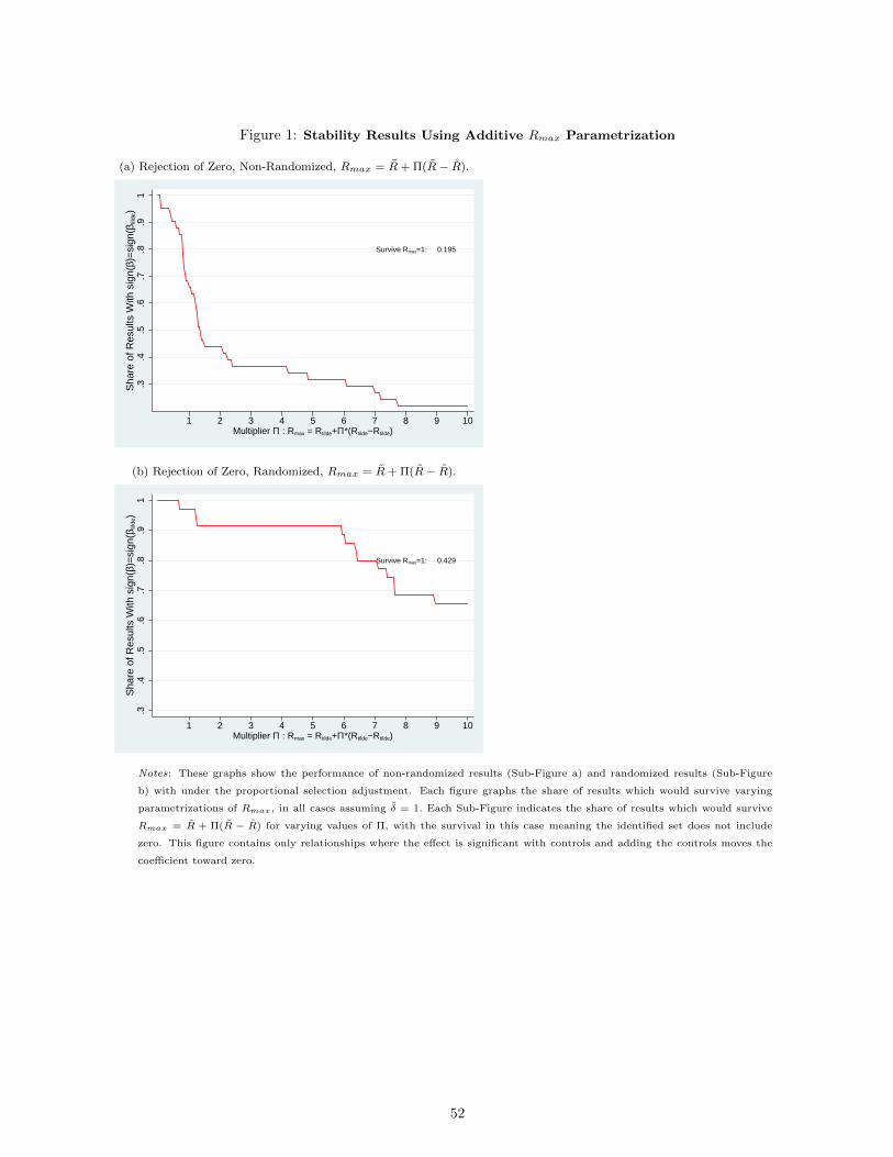
Figure 1: Stability Results Using Additive Rmax Parametrization

(a) Rejection of Zero, Non-Randomized, Rmax = R+ Π(R− R).

Survive Rmax=1: 0.195

.3.4

.5.6

.7.8

.91

Sha

re o

f Res

ults

With

sig

n(β)

=si

gn(β

tilde

)

1 2 3 4 5 6 7 8 9 10Multiplier Π : Rmax = Rtilde+Π*(Rtilde−Rtilde)

(b) Rejection of Zero, Randomized, Rmax = R+ Π(R− R).

Survive Rmax=1: 0.429

.3.4

.5.6

.7.8

.91

Sha

re o

f Res

ults

With

sig

n(β)

=si

gn(β

tilde

)

1 2 3 4 5 6 7 8 9 10Multiplier Π : Rmax = Rtilde+Π*(Rtilde−Rtilde)

Notes: These graphs show the performance of non-randomized results (Sub-Figure a) and randomized results (Sub-Figure

b) with under the proportional selection adjustment. Each figure graphs the share of results which would survive varying

parametrizations of Rmax, in all cases assuming δ = 1. Each Sub-Figure indicates the share of results which would survive

Rmax = R + Π(R − R) for varying values of Π, with the survival in this case meaning the identified set does not include

zero. This figure contains only relationships where the effect is significant with controls and adding the controls moves the

coefficient toward zero.

52