Spectral Coefficient Analysis on GeometericalDeformation using Laplace-Beltrami Operator

An Undergraduate ThesisSubmitted to the Department of Mechanical Engineering

The Ohio State UniversityIn Partial Fulfillment of the Requirements for Graduation with Distinction in Mechanical

Engineering

Skylar Sible

Defense Committe:

Dr. Shawn Midlam-Mohler, Advisor

Dr. Sheng Dong

April 16, 2020

Contents

1 Introduction 1

1.1 Background and motivation . . . . . . . . . . . . . . . . . . . . . . . . . . . 1

1.2 Related Research . . . . . . . . . . . . . . . . . . . . . . . . . . . . . . . . . 3

2 Mathematical Concepts 5

2.1 Laplace-Beltrami Operator . . . . . . . . . . . . . . . . . . . . . . . . . . . . 5

2.2 Spectral Coefficients . . . . . . . . . . . . . . . . . . . . . . . . . . . . . . . 9

3 Workflow 11

3.1 Pre-processsing . . . . . . . . . . . . . . . . . . . . . . . . . . . . . . . . . . 13

3.2 Simulation . . . . . . . . . . . . . . . . . . . . . . . . . . . . . . . . . . . . . 13

3.3 Post-processing . . . . . . . . . . . . . . . . . . . . . . . . . . . . . . . . . . 14

3.3.1 Method for determining representative eigenvectors based on targetdeformation . . . . . . . . . . . . . . . . . . . . . . . . . . . . . . . . 15

3.3.2 Database filtration using cosine similarity . . . . . . . . . . . . . . . 17

3.4 Evaluation . . . . . . . . . . . . . . . . . . . . . . . . . . . . . . . . . . . . . 17

4 Results 18

5 Conclusion 24

5.1 Contributions . . . . . . . . . . . . . . . . . . . . . . . . . . . . . . . . . . . 24

5.2 Additional applications . . . . . . . . . . . . . . . . . . . . . . . . . . . . . . 25

ii

5.3 Future work . . . . . . . . . . . . . . . . . . . . . . . . . . . . . . . . . . . . 25

5.4 Summary . . . . . . . . . . . . . . . . . . . . . . . . . . . . . . . . . . . . . 25

A START.m 27

A.1 read dataviewer.m . . . . . . . . . . . . . . . . . . . . . . . . . . . . . . . . 31

A.2 mesh geometry.m . . . . . . . . . . . . . . . . . . . . . . . . . . . . . . . . . 32

A.3 Laplace Beltrami Operator.m . . . . . . . . . . . . . . . . . . . . . . . . . . 34

A.4 d3plot read.m . . . . . . . . . . . . . . . . . . . . . . . . . . . . . . . . . . . 36

A.5 Spec coeff.m . . . . . . . . . . . . . . . . . . . . . . . . . . . . . . . . . . . . 38

A.6 deformation modes.m . . . . . . . . . . . . . . . . . . . . . . . . . . . . . . . 39

A.7 time frequency cluster.m . . . . . . . . . . . . . . . . . . . . . . . . . . . . . 49

A.8 important eigenvectors.m . . . . . . . . . . . . . . . . . . . . . . . . . . . . . 57

A.8.1 scale evecs.m . . . . . . . . . . . . . . . . . . . . . . . . . . . . . . . 60

A.9 similarity.m . . . . . . . . . . . . . . . . . . . . . . . . . . . . . . . . . . . . 61

A.10 reconstruction comparison all.m . . . . . . . . . . . . . . . . . . . . . . . . . 63

A.11 plot final timestep.m . . . . . . . . . . . . . . . . . . . . . . . . . . . . . . . 66

iii

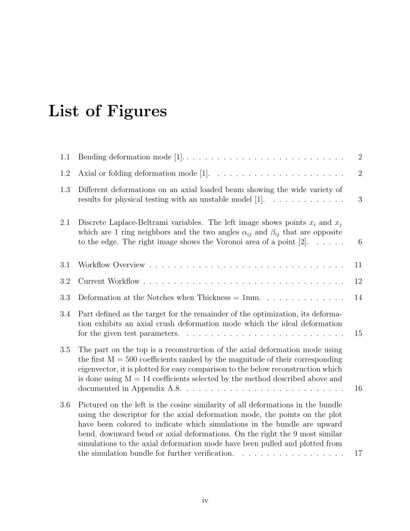
List of Figures

1.1 Bending deformation mode [1]. . . . . . . . . . . . . . . . . . . . . . . . . . . 2

1.2 Axial or folding deformation mode [1]. . . . . . . . . . . . . . . . . . . . . . 2

1.3 Different deformations on an axial loaded beam showing the wide variety ofresults for physical testing with an unstable model [1]. . . . . . . . . . . . . 3

2.1 Discrete Laplace-Beltrami variables. The left image shows points xi and xjwhich are 1 ring neighbors and the two angles αij and βij that are oppositeto the edge. The right image shows the Voronoi area of a point [2]. . . . . . 6

3.1 Workflow Overview . . . . . . . . . . . . . . . . . . . . . . . . . . . . . . . . 11

3.2 Current Workflow . . . . . . . . . . . . . . . . . . . . . . . . . . . . . . . . . 12

3.3 Deformation at the Notches when Thickness = 1mm. . . . . . . . . . . . . . 14

3.4 Part defined as the target for the remainder of the optimization, its deforma-tion exhibits an axial crush deformation mode which the ideal deformationfor the given test parameters. . . . . . . . . . . . . . . . . . . . . . . . . . . 15

3.5 The part on the top is a reconstruction of the axial deformation mode usingthe first M = 500 coefficients ranked by the magnitude of their correspondingeigenvector, it is plotted for easy comparison to the below reconstruction whichis done using M = 14 coefficients selected by the method described above anddocumented in Appendix A.8. . . . . . . . . . . . . . . . . . . . . . . . . . . 16

3.6 Pictured on the left is the cosine similarity of all deformations in the bundleusing the descriptor for the axial deformation mode, the points on the plothave been colored to indicate which simulations in the bundle are upwardbend, downward bend or axial deformations. On the right the 9 most similarsimulations to the axial deformation mode have been pulled and plotted fromthe simulation bundle for further verification. . . . . . . . . . . . . . . . . . 17

iv

4.1 The top shows a reconstruction using M = 500 eigenvectors based on themagnitude of their corresponding eigenvalue. The middle row represents re-construction from the proposed descriptor with sizes M = 14 for axial crush,M = 17 for upward bend, M = 16 for downward bend. The bottom row showsa reconstruction using M = 14 for axial crush, M = 17 for upward bend,M = 16 for downward bend however these eigenvectors are sorted using thetraditional method rather than the proposed descriptor. . . . . . . . . . . . 19

4.2 Normalized cosine similarity plot for upward bend deformation mode. X axisis the simulation, and y axis is similarity where 1 is equal to 100 percentsimilarity. Points closest to the X axis represent simulations with highestsimilarity to the deformation mode. . . . . . . . . . . . . . . . . . . . . . . 20

4.3 Normalized cosine similarity plot for downward bend deformation mode. Xaxis is the simulation, and y axis is similarity where 1 is equal to 100 percentsimilarity. Points closest to the X axis represent simulations with highestsimilarity to the deformation mode. . . . . . . . . . . . . . . . . . . . . . . 20

4.4 Normalized cosine similarity plot for axial deformation mode. X axis is thesimulation, and y axis is similarity where 1 is equal to 100 percent similarity.Points closest to the X axis represent simulations with highest similarity tothe deformation mode. . . . . . . . . . . . . . . . . . . . . . . . . . . . . . . 21

4.5 The y-axis is the spectral coefficients ordered by the magnitude of their cor-responding eigenvalue, the x-axis is the time-steps 1-20 of the model part forthe upwards bending deformation mode. All coefficients above the mean areplotted in white and all others in black. The coefficients above the mean areconsidered the driving coefficients for this specific deformation mode, howeverin this research only coefficients 2 standard deviations above the mean arepart of the descriptor. . . . . . . . . . . . . . . . . . . . . . . . . . . . . . . 22

4.6 The y-axis is the spectral coefficients ordered by the magnitude of their corre-sponding eigenvalue, the x-axis is the time-steps 1-20 of the model part for thedownwards bending deformation mode. All coefficients above the mean areplotted in white and all others in black. The coefficients above the mean areconsidered the driving coefficients for this specific deformation mode, howeverin this research only coefficients 2 standard deviations above the mean arepart of the descriptor. . . . . . . . . . . . . . . . . . . . . . . . . . . . . . . 22

4.7 The y-axis is the spectral coefficients ordered by the magnitude of their cor-responding eigenvalue, the x-axis is the time-steps 1-20 of the model part forthe axial deformation mode. All coefficients above the mean are plotted inwhite and all others in black. The coefficients above the mean are consideredthe driving coefficients for this specific deformation mode, however in this re-search only coefficients 2 standard deviations above the mean are part of thedescriptor. . . . . . . . . . . . . . . . . . . . . . . . . . . . . . . . . . . . . . 23

v

Abstract

Automotive part design consists of crash simulation and design optimization done by

finite-element computing software. In order to make these processes possible, the part

geometry must be efficiently represented. Different parameters can be defined in an

optimization in order to determine appropriate material models and part thickness,

however there are still computational limitations on optimizing based on specific part

deformation. This paper proposes a method that goes beyond tracking individual node

displacements in order to use deformation as a parameter for optimized part design. Using

a dimension reduction method, deformations of the part can be classified using a spectral

descriptor corresponding to that deformation. This spectral descriptor is taken a step

further and is used to efficiently filter a simulation bundle based on the defined desired

geometric deformation. In addition, this spectral descriptor is used for part reconstruction

with a higher visual accuracy compared to traditional reconstruction methods. Finally, this

paper proposes application of this method into design optimization using a machine

learning approach.

Keywords: design optimization, dimension reduction, part deformation, spectral

descriptor

Acknowledgments

I would like to thank Shawn Midlam-Mohler for advising this research project. I would also

like to thank Patricia Wollstadt and Nicola Aulig for their mentorship during my

internship at HRI-EU, where this research began. I would like to thank Rodrigo Iza-Teran

for allowing me to use the Dataviewer software at the onset of this research project. Lastly

i would like to thank Emily Nutwell for allowing me to use part of her LS-Dyna hat section

model for the simulations run in this thesis.

i

Chapter 1

Introduction

1.1 Background and motivation

Advancements of computational analysis have replaced physical crash testing. This has

made a huge impact on the automotive industry, and will continue to improve the

automotive design process, by reducing cost and time, and improving efficiency and safety.

Finite element analysis is utilized in order to achieve all of these goals. When an engineer

is designing a part, they must consider all the different solutions to accomplish their given

goal. A central goal is achieving specific deformations under different crash scenarios, i.e.

crashworthiness. This paper explores the need for engineers to design parts with very

specific physical deformations in different crash scenarios.

In his book, Hesham Kamel Ibrahim defines crashworthiness as the process of improving

the crash performance of a structure by sacrificing it under impact for the purpose of

protecting occupants from injuries [3]. Crashworthiness can be improved by increasing the

energy absorption and influencing the deformation mode of the part. This results in

reducing the impact on the occupants and protects the other parts in the assembly.

1

Because the energy absorption is greatly effected by the deformation, influencing certain

deformation modes can be a powerful design tool. The areas in the vehicle designed to

absorb the energy, or load, of the impact can be defined as crumple zones. The crumple

zones protect the crashworthiness of a vehicle by deforming in a way that optimizes the

amount of energy absorbed and the severity of the damage to the rest of the vehicle and

occupants. The two types of deformation focused on in this paper are axial deformation,

also known as folding deformation, and bending deformation as shown in Figures 1.1 and

1.2.

Figure 1.1: Bending deformation mode [1].

Figure 1.2: Axial or folding deformation mode [1].

When it comes to energy absorption in a crumple zone, a part undergoing an axial

deformation is most effective. Due to instabilities it is difficult to achieve axial deformation,

and often bending is the result of a failed axial deformation mode [1]. In other scenarios

bending at a local hinge is desired to protect passengers, or other parts of the vehicle.

Often this bending mode fails by a bending deformation occurring at an undesired local

hinge. When structural parts are put under a compressive load, deformations can easily

become irregular, or unstable, this causes a loss in energy absorption. A loss in energy

absorption, may completely alter the crash behavior of the entire system. Examples of

2

these instabilities are shown in Figure 1.3, certain conditions must be met prior to a crash

in order to achieve the desired deformation, slight differences in these conditions result in a

high variance in crash results, in a complex system this will cause an undesired chain

reaction effecting the entire model. Paul Du Bois stresses in his paper, ’Vehicle

Crashworthiness and Occupant Protection’, that the need to understand the triggers

causing instabilities is critical in order to design countermeasures to prevent them [1].

Figure 1.3: Different deformations on an axial loaded beam showing the wide variety of resultsfor physical testing with an unstable model [1].

1.2 Related Research

Advancements in computational analysis has improved the design process of crumple zones

however there are still limitations. The finite element method (FE method) does not

replace the need for physical testing entirely, but it is an extremely useful tool to narrow

down the different design options, leaving just a few for prototyping and physical

verification. The FE method, in most cases, will have infeasible computational costs

without the help of a design of experiments (DOE) technique. With the use of a

meta-model and DOE technique, the number of samples can be dramatically decreased to

only simulate parameters achieving certain results. For example, a DOE could be utilized

3

to only test material parameters that achieve the minimum energy absorption for the

model. There is a lot of research covering this topic, and these techniques are widely used

in industry today.

This technique has its limitations, it happens often that the parameters providing the

optimal numerical results do not provide the desired deformation mode. In other cases,

even with the desired deformation of the part in question, this may result in an undesired

chain reaction to the rest of the assembly, causing other parts to fail. When this occurs it

can be extremely time consuming to open the result files for each simulation result to

inspect the geometrical deformations to verify success.

Rodrigo Iza Teran has developed a very useful solution to this problem. In his research he

uses dimension reduction methods and spectral decomposition to provide a new way to

post-process simulation bundle results [6]. The dataviewer tool, programmed by the

Fraunhofer institute SCAI, implements his research into a tool for engineers. This tool

loads the resulting geometries of the complete simulation bundle so one could quickly see if

the desired deformation was achieved. In addition it uses spectral decomposition to classify

different results by certain spectral coefficients. This can be used for clustering results and

can help one conclude what parameters could be triggering different deformation modes.

Use of spectral decomposition for geometric classification isn’t a widely researched topic.

Spectral classification is used in image processing and is used on meshes for feature

detection and database retrieval as discussed in []. The related research for use of spectral

decomposition for engineering applications is even more limited. Although limited, the

small amount of research in this area is extremely promising and could greatly impact the

efficiency of engineering techniques used in industry today.

The research in this paper explores the use of a spectral decomposition in order to optimize

the FE method with respect to specific deformation modes.

4

Chapter 2

Mathematical Concepts

The following section will propose the mathematical concepts used as the foundation for

the following research. In order to do a spectral decomposition of a geometry one must first

preform dimension reduction. The eigen-decomposition must be preformed on a square

matrix where the size is equal to [n× n] where n is equal to the number of points on the

surface (nodes). This matrix is a ’database’ containing all the information about the

relationships between two points. Dimension reduction methods are used to create the

’database’ considered for spectral decomposition. There are many different dimension

reduction methods however, the method for dimension reduction used in the following

research is the Laplace-Beltrami method, or Laplician for short.

2.1 Laplace-Beltrami Operator

The Laplace-Beltrami operator is the divergence of the gradient [2],

∆f = div grad f, (2.1)

5

The Laplace-Beltrami method depends on distances measured between points on a surface.

This applies nicely to surface meshes because they are constructed by a set of points

(nodes) that when connected represent a shape. By using this method effectively the

shape, also known as a differential geometry, will be represented as a 2D manifold in R3

space. There are a number of different schemes for the discrete Laplacian, the following

section will introduce two of them. The first being the cotangent scheme and the second

being the Belkin scheme.

The cotangent scheme is widely used in computer graphics, it is a discrete

Laplace-Beltrami operator that focuses on the 1-ring neighborhood of a point. This means

that the following equation is used to computed the discrete Laplacian for each set of

adjacent nodes on a mesh. This discrete operator K is defined by [4]

K(xi) =1

2Ai

∑xjεN(xi)

(cotαij + cotβij)(xi − xj), (2.2)

Where Ai is the Voronoi region area of xi, Ni is the single 1 ring neighborhood around

point xi. The line connecting points xi and xj is defined as an edge and αij and βij are

angles opposite to the edge as seen in Figure 2.1.

Figure 2.1: Discrete Laplace-Beltrami variables. The left image shows points xi and xj whichare 1 ring neighbors and the two angles αij and βij that are opposite to the edge. The right imageshows the Voronoi area of a point [2].

The Voronoi region is calculated by,

6

Ai =1

8

∑jεN(xi)

(cotαij + cotβij)‖ xi − xj ‖2, (2.3)

The cotangent scheme has shown to produce non-symmetric matrices resulting in complex

eigenvectors, meaning it can’t be used in applications depending on the eigenstructure for

geometrical operations [5]. By using angles the cotangent scheme is in return heavily

influenced by the geometry of the triangles, or the geometry of the mesh. Another

limitation of the method is there isn’t a clear method to extend point-point calculations

beyond one neighborhood around the point.

The Belkin scheme proposes a mesh Laplacian operator LhM , where M is a mesh and h

corresponds to the size of the neighborhood at a point. This means the operator is not

constrained by only adjacent node pairs and is not influenced by the geometry of the

elements. This means it works with faces made up of any number of vertices, and

theoretically would also work with meshes containing mixed element types (i.e. tri, quad,

or mixed elements).

LhMf(x) =1

4πh2

∑tεM

Area(t)

#t

∑yεV (t)

e−‖x−y‖2

4h (f(y)− f(x)), (2.4)

where t is defined as a face on the mesh M and #t refers to the number of vertices on t.

This scheme is independent of the geometry of the mesh, and considers all node pairs in

the mesh. Node pairs with distances exceeding the size of the defined neighborhood are not

considered in the approximation for this method. The method for approximation is defined

in algorithm 1 and in appendix A.3.

7

Algorithm 1: Belkin Scheme

input : Vertices, V , with size n× 3, where n = number of vertices.

Faces, F , with size f × p, where f = number of faces and p = vertices per face.

output: Eigenvectors, Evecs

begin

1 foreach F do

2 foreach V εF do

3 AV = Area(F )p

4 foreach Vi do

5 foreach Vj do

6 dij = dist(Vi, Vj) ;

7 if dij > (ρ√h) then

8 L(i, j) = ( 14πh2

)(Ai)(Aj)(e−

d2ij4h )

else

9 L(i, j) = 0

10 L(i, i) = −∑L(i, :) ;

11 Evecs = Eigs(L)

The result of the Laplace-Beltrami operator is a square matrix that’s size is equivalent to

the number of nodes on the mesh. From the square matrix eigenvectors, λ, and

eigenvalues, ψ, are calculated, which must satisfy the following equation,

∆Mψ = −λψ, (2.5)

where ∆M is the Laplace-Beltrami operator on manifold M .

Due to the high nodal count in typical Finite Element Analysis (FEA) calculations, only a

8

subset of eigenvectors will be considered. This is justified due to related research showing

that only a subset of eigenvectors are needed for reconstruction, Rodrigo Iza Teran

proposes that accuracy of the reconstruction increases as the number of eigenvectors used

for reconstruction increases. He also proposes that after a certain amount of eigenvectors,

the increased accuracy for each additional eigenvector is not worth the added

computational cost. He suggests 100 eigenfunctions for reconstruction as the optimal

amount for the application studied in his thesis []. Due to the similarity of his application

to the one in this paper, 100 eigenvectors will be considered, as well as 500 for comparison.

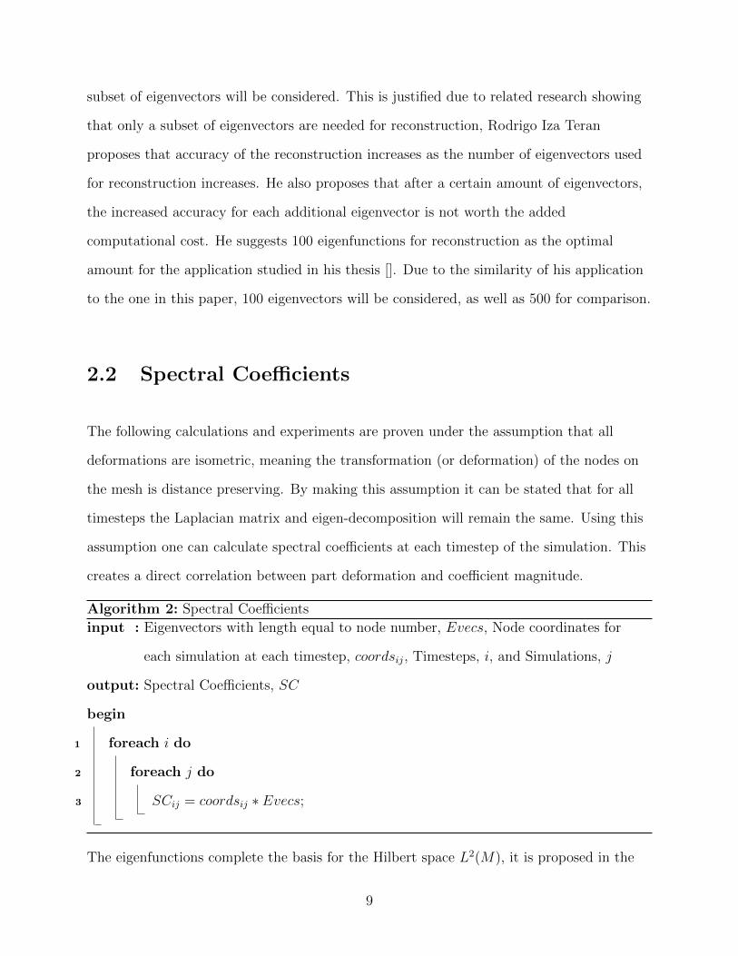
2.2 Spectral Coefficients

The following calculations and experiments are proven under the assumption that all

deformations are isometric, meaning the transformation (or deformation) of the nodes on

the mesh is distance preserving. By making this assumption it can be stated that for all

timesteps the Laplacian matrix and eigen-decomposition will remain the same. Using this

assumption one can calculate spectral coefficients at each timestep of the simulation. This

creates a direct correlation between part deformation and coefficient magnitude.

Algorithm 2: Spectral Coefficients

input : Eigenvectors with length equal to node number, Evecs, Node coordinates for

each simulation at each timestep, coordsij, Timesteps, i, and Simulations, j

output: Spectral Coefficients, SC

begin

1 foreach i do

2 foreach j do

3 SCij = coordsij ∗ Evecs;

The eigenfunctions complete the basis for the Hilbert space L2(M), it is proposed in the

9

book ’Diffusion-Driven Wavelet Design for Shape Analysis’ that for manifolds without

boundaries and for manifolds with Neumann-conditioned boundaries, that the first

eigenvalue is equal to zero, λ0 = 0 and that the first eigenfunction is constant everywhere

on the manifold,

ψ0(x) =1√µ(M)

. (2.6)

This eliminates the need to set fixed values for eigenfunctions at the boundary [3].

10

Chapter 3

Workflow

The workflow consists of three main stages, pre-processing, simulation, and

post-processing. The pre-processing stage consists of calculations from the undeformed

mesh, then in the second stage, an optimization is preformed to obtain a simulation

bundle. The majority of steps are in the final stage, post-processing.

Aside from the te simulation bundles calculated using LS-Opt, the other calculations are

done using the MATLAB code documented in Appendix A.

pre-processing

running simulation/optimization

post-processing

Figure 3.1: Workflow Overview

11

Laplace-beltrami operator on undeformed mesh

solve the eigenvalue problem to obtain eigen-

vectors from the laplace-beltrami matrix

compute a simulation bundle that con-

sists of many different deformation modes

select the desired deformation

mode from the simulation bundle

calculate the spectral coefficients of all the sim-

ulations in the bundle at their final timestep

choose important coefficients using the spectral

coeffients from the desired deformation mode

verify selection with reconstruction

change

selection

parameters

does the

reconstruction

represent the

desired

deformation?

cosine similarity of selected coef-

ficients to the simulation bundle

no

yes

Figure 3.2: Current Workflow

12

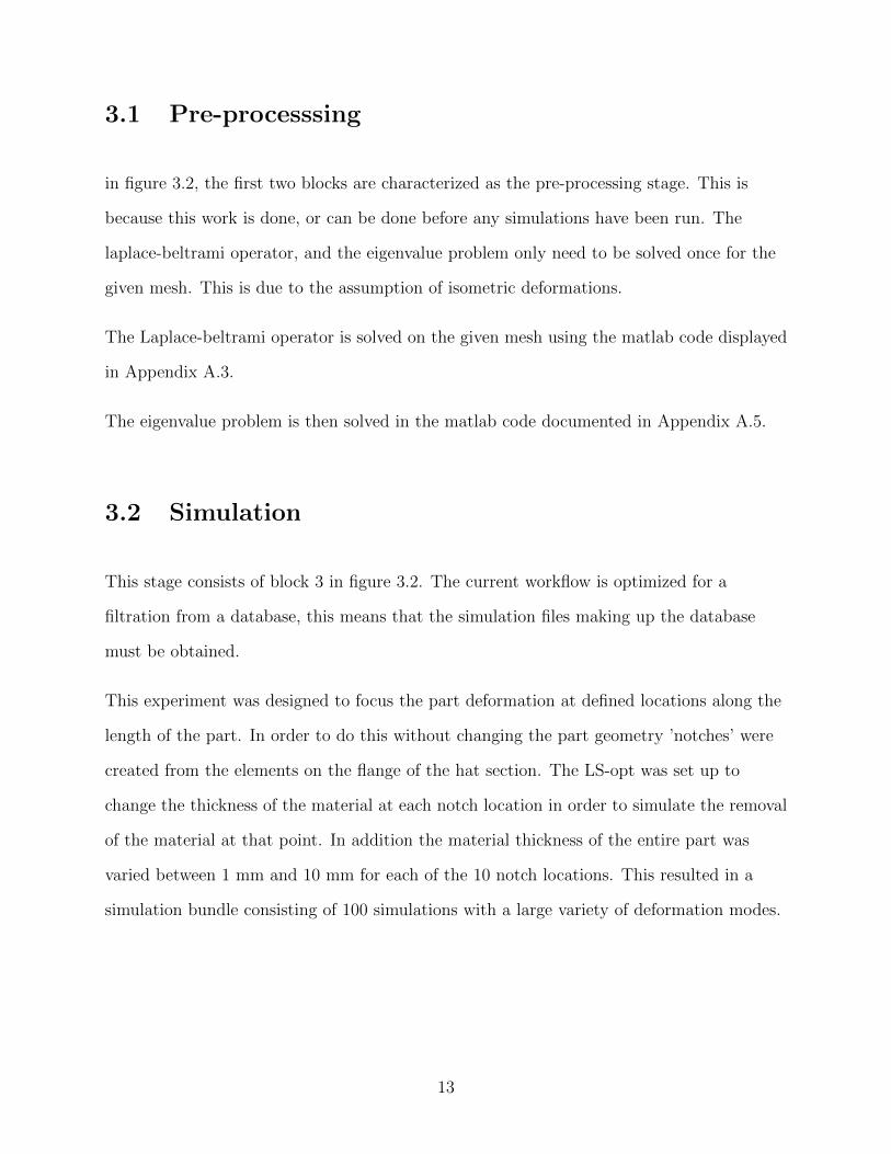
3.1 Pre-processsing

in figure 3.2, the first two blocks are characterized as the pre-processing stage. This is

because this work is done, or can be done before any simulations have been run. The

laplace-beltrami operator, and the eigenvalue problem only need to be solved once for the

given mesh. This is due to the assumption of isometric deformations.

The Laplace-beltrami operator is solved on the given mesh using the matlab code displayed

in Appendix A.3.

The eigenvalue problem is then solved in the matlab code documented in Appendix A.5.

3.2 Simulation

This stage consists of block 3 in figure 3.2. The current workflow is optimized for a

filtration from a database, this means that the simulation files making up the database

must be obtained.

This experiment was designed to focus the part deformation at defined locations along the

length of the part. In order to do this without changing the part geometry ’notches’ were

created from the elements on the flange of the hat section. The LS-opt was set up to

change the thickness of the material at each notch location in order to simulate the removal

of the material at that point. In addition the material thickness of the entire part was

varied between 1 mm and 10 mm for each of the 10 notch locations. This resulted in a

simulation bundle consisting of 100 simulations with a large variety of deformation modes.

13

Figure 3.3: Deformation at the Notches when Thickness = 1mm.

3.3 Post-processing

The first step in the post-processing stage is to manually set a deformation target. This

target corresponds to the ideal geometric deformation that the code will in turn use to

return additional simulations with similar deformations. For this research application this

step is done by visual inspection, this is done under the assumption that the engineer

preforming the optimization knows how the part should be deforming with the giving test

parameters defined in the simulation stage of this workflow.

14

The target deformation defined for this research is a part exhibiting an axial crush in the

center of the beam, this ideal deformation is pictured below in figure 3.4

Figure 3.4: Part defined as the target for the remainder of the optimization, its deformationexhibits an axial crush deformation mode which the ideal deformation for the given test parameters.

The Cartesian coordinates for the nodes at each timestep of the simulations in the bundle

are read from the d3plot files using the MATLAB code documented in Appendix A.4.

These node locations are then used to calculate the spectral coefficients for all simulations

in the bundle at each timestep. This spectral data is used to calculate the representative

eigenvectors in the desired deformation mode.

3.3.1 Method for determining representative eigenvectors based

on target deformation

The representative eigenvectors are determined by calculating which eigenvectors deviate

from the mean in the X, Y and Z directions. This is done by first taking the mean and

standard deviation of the X, Y, and Z coefficients respectively. The important coefficients

are then defined as the coefficients that are 2 standard deviations above the mean

coefficient value.

The eigenvectors are then scaled by the by the important coefficients, the sum of these

scaled eigenvectors is used for reconstruction.

15

Figure 3.5: The part on the top is a reconstruction of the axial deformation mode using the firstM = 500 coefficients ranked by the magnitude of their corresponding eigenvector, it is plotted foreasy comparison to the below reconstruction which is done using M = 14 coefficients selected bythe method described above and documented in Appendix A.8.

Based on the reconstruction pictured in Figure 3.5 the selected M = 14 important

coefficients are determined effective for a low dimensional representation of the target

deformation mode.

If this was not determined an effective representative this is were the iteration step

pictured in Figure 3.2 would occur. The coefficients could be adjusted by selecting

everything 1 standard deviation above the mean, or all values above the mean. If the

number of coefficients, M, are too high than the value could be adjusted to be 3 standard

deviations above the mean or higher. For the purpose of this research, 2 standard

deviations have been determined sufficient for representation of this deformation.

16

3.3.2 Database filtration using cosine similarity

After visual verification, the same important coefficients will be filtered out of all

simulations in the bundle and the same reconstructive eigenvector is calculated. Using the

reconstruction vector for the target deformation mode, cosine similarity is calculated

between it an every other simulation in the bundle. This step is documented in Appendix

A.9.

Figure 3.6: Pictured on the left is the cosine similarity of all deformations in the bundle usingthe descriptor for the axial deformation mode, the points on the plot have been colored to indicatewhich simulations in the bundle are upward bend, downward bend or axial deformations. On theright the 9 most similar simulations to the axial deformation mode have been pulled and plottedfrom the simulation bundle for further verification.

3.4 Evaluation

Based on the verification above the workflow defined is effective in determining important

spectral coefficients as they pertain to a specific deformation mode. These coefficients are

then used to do a low dimensional reconstruction of the part. Further analysis allows one

to use these coefficients as a target for a database filtration.

17

Chapter 4

Results

Using the spectral coefficients for a low dimensional reconstruction isn’t novel, however

traditionally the reconstruction is done using the first M eigenvectors based on the

magnitude of their corresponding eigenvalue. This is effective in construction high

frequency geometric features however details are compromised in this method. The fine

details are important when considering specific deformation modes. In order to evaluate

the results of the workflow outlined in Chapter 3, reconstruction method for all 3

deformation modes are used for comparison.

18

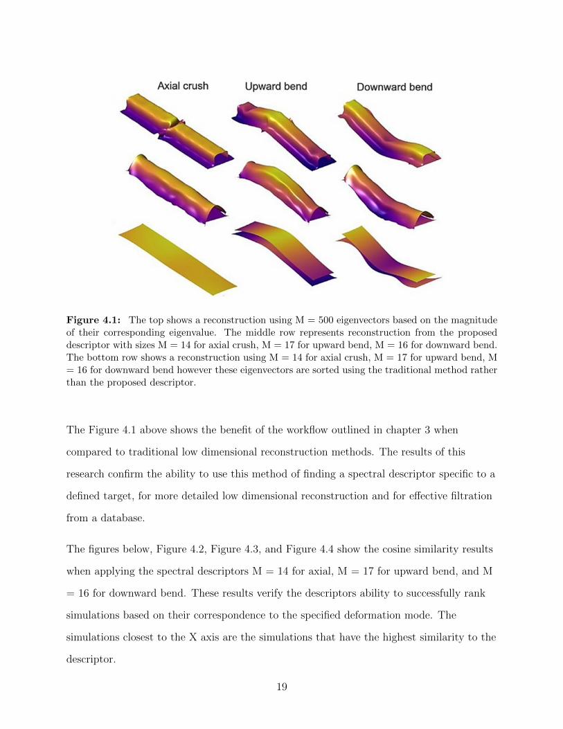
Figure 4.1: The top shows a reconstruction using M = 500 eigenvectors based on the magnitudeof their corresponding eigenvalue. The middle row represents reconstruction from the proposeddescriptor with sizes M = 14 for axial crush, M = 17 for upward bend, M = 16 for downward bend.The bottom row shows a reconstruction using M = 14 for axial crush, M = 17 for upward bend, M= 16 for downward bend however these eigenvectors are sorted using the traditional method ratherthan the proposed descriptor.

The Figure 4.1 above shows the benefit of the workflow outlined in chapter 3 when

compared to traditional low dimensional reconstruction methods. The results of this

research confirm the ability to use this method of finding a spectral descriptor specific to a

defined target, for more detailed low dimensional reconstruction and for effective filtration

from a database.

The figures below, Figure 4.2, Figure 4.3, and Figure 4.4 show the cosine similarity results

when applying the spectral descriptors M = 14 for axial, M = 17 for upward bend, and M

= 16 for downward bend. These results verify the descriptors ability to successfully rank

simulations based on their correspondence to the specified deformation mode. The

simulations closest to the X axis are the simulations that have the highest similarity to the

descriptor.

19

Figure 4.2: Normalized cosine similarity plot for upward bend deformation mode. X axis is thesimulation, and y axis is similarity where 1 is equal to 100 percent similarity. Points closest to theX axis represent simulations with highest similarity to the deformation mode.

Figure 4.3: Normalized cosine similarity plot for downward bend deformation mode. X axis isthe simulation, and y axis is similarity where 1 is equal to 100 percent similarity. Points closest tothe X axis represent simulations with highest similarity to the deformation mode.

20

Figure 4.4: Normalized cosine similarity plot for axial deformation mode. X axis is the simulation,and y axis is similarity where 1 is equal to 100 percent similarity. Points closest to the X axisrepresent simulations with highest similarity to the deformation mode.

In Figure 4.2 the blue dots, or upward simulations, show curvature withing the different

notch increments. For example, simulations 1-10 correspond to a specific notch with

thicknesses increasing by 1mm in each simulation. These curves indicate that for most of

the notch locations, part thickness equal to 4mm results in an upward bend. This

information would then be valuable to an engineer wishing to obtain an upward bend

deformation mode.

The next set of figures plotted below are binary plots of the coefficients for the

representative deformation modes. The Y axis is the coefficients 1-500 and they are ordered

by the magnitude of their corresponding eigenvalue. The X axis is time-steps of the

simulation 0-20. The purpose of these plots is to see if coefficients in the higher frequency

range are above the mean for specific deformation modes. Also the time-step was plotted

to see if certain coefficients passed the mean threshold as the part continued to deform, in

addition to coefficients dropping below the threshold as the part deformation progresses.

21

Figure 4.5: The y-axis is the spectral coefficients ordered by the magnitude of their correspondingeigenvalue, the x-axis is the time-steps 1-20 of the model part for the upwards bending deformationmode. All coefficients above the mean are plotted in white and all others in black. The coefficientsabove the mean are considered the driving coefficients for this specific deformation mode, howeverin this research only coefficients 2 standard deviations above the mean are part of the descriptor.

Figure 4.6: The y-axis is the spectral coefficients ordered by the magnitude of their correspond-ing eigenvalue, the x-axis is the time-steps 1-20 of the model part for the downwards bendingdeformation mode. All coefficients above the mean are plotted in white and all others in black.The coefficients above the mean are considered the driving coefficients for this specific deformationmode, however in this research only coefficients 2 standard deviations above the mean are part ofthe descriptor.

22

Figure 4.7: The y-axis is the spectral coefficients ordered by the magnitude of their correspondingeigenvalue, the x-axis is the time-steps 1-20 of the model part for the axial deformation mode. Allcoefficients above the mean are plotted in white and all others in black. The coefficients abovethe mean are considered the driving coefficients for this specific deformation mode, however in thisresearch only coefficients 2 standard deviations above the mean are part of the descriptor.

The binary plots confirm the assumption that certain coefficients become either more

prominent as deformation progresses or less prominent. In addition the figures above,

Figure 4.5, Figure 4.6, and Figure 4.7 show that certain high frequency coefficients are

prominent on specific modes. This verifies that the coefficients to best represent the

deformation mode are not necessarily correlated to the magnitude of the eigenvalue, rather

than their magnitude in comparison to the other coefficients. The coefficients deviating the

furthest from the mean indicate high importance in the geometry of the designated

deformation mode.

23

Chapter 5

Conclusion

Advancements in computational simulation have reduced costly and time consuming

physical crash testing. Currently simulation is still limited by certain things. There is

currently no way to define a complex deformation mode in a FEA analysis. There are

methods engineers use to track individual node displacements however complicated

deformation modes such as folding or twisting cannot be easily tracked by individual nodes.

The purpose of this research is to develop a method that can be used to sort through

simulation files to find all simulation results with the desired deformation mode. This is

important for automotive engineering applications because in addition to other parameters

in crash testing, physical deformation should be preserved in order to optimize the

crashworthiness of the vehicle.

5.1 Contributions

The research in this paper has contributed to te scientific community by presenting a novel

way to use spectral descriptors to define a deformation mode in order to do low

24

dimensional reconstructions and database filtration.

5.2 Additional applications

This method could also be applied in computer graphics in order to make visually accurate

low dimensional reconstructions. In the engineering domain there are endless applications

in finite element simulation and part optimization. Another interesting application of this

research would be to preserve different deformation modes when calculating a topology

optimization.

5.3 Future work

The future work on the research project would be to incorporate this method into a

simulation optimization. This descriptor would be used as parameter in a machine learning

optimization approach. Another study that would further validate this method would

include a robustness study with different part geometries and deformation modes.

5.4 Summary

To summarize the research above, a method was developed to used spectral analysis of part

deformations in order to come up with a spectral descriptor that represents a complex

deformation mode. The importance of this spectral descriptor is to be able to define a

deformation mode during a design optimization, or filter through a simulation bundle to

find results matching the target deformation mode.

25

Bibliography

[1] Paul Du Bois, Clifford C. Chou, Bahig B. Fileta, Tawfik B. Khalil, Albert I. King,

Hikmat F. Mahmood, Harold J. Mertz, Jac Wismans, Priya Prasad, and Jamel E.

Belwafa. Vehicle crashworthiness and occupant protection.

[2] Tingbo Hou and Hong Qin. Diffusion-driven Wavelet Design for Shape Analysis. AK

Peters/CRC Press, 2014.

[3] Hesham Kamel Ibrahim. Design optimization of vehicle structures for crashworthiness

improvement. Citeseer, 2009.

[4] Mark Meyer, Mathieu Desbrun, Peter Schroder, and Alan H Barr. Discrete

differential-geometry operators for triangulated 2-manifolds. 2001.

[5] Fabiano Petronetto, Afonso Paiva, Elias S Helou, DE Stewart, and Luis Gustavo

Nonato. Mesh-free discrete laplace–beltrami operator. In Computer Graphics Forum,

volume 32, pages 214–226. Wiley Online Library, 2013.

[6] Rodrigo Iza Teran and Jochen Garcke. Geometrical methods for the analysis of

simulation bundles. Doktorarbeit, Universitat Bonn, eingereicht, 2016.

26

Appendix A

START.m

1 % Skylar S i b l e HRI−EU 14 .12 .2018

2

3 c l c

4 c l e a r

5

6 %START HERE Update appropr ia te va lues

7

8 % Fuct ions writen by Skylar S i b l e at HRI−EU

9 addpath ( ’ f unc t i on s ’ )

10

11 addpath ( ’ f unc t i on s / functionsRough ’ )

12

13 % Fuction wr i t t en by other s copied from open source webs i t e s

14 addpath ( ’ f unc t i on s /Borrowed Functions ’ )

15

16

17 load ( ’C:\ Users\Skylar\SkyDrive\Documents\Research\mesh data .mat ’ )

18 %% In s e r t appropr ia te va lues below : Al l these va lues should be updated p r i o r to running the code

19 %

20 % % Path to dataviewer f i l e s , s ee examples below

21 %

22 % % Hat s e c t i on and Bottom p la t e with notches inc luded

23 % path = ’/ h r i / l o c a l d i s k / s s i b l e / da tav i ewe rp ro j e c t s /BeamCrush .100 samples . withnotch / f i l e / ’ ;

24 %

25 % % Hat s e c t i on alone , with notches inc luded ( t h i s would r e s u l t in IP =

26 % % 1 , see below f o r d e t a i l s

27 % % path = ’/ h r i / l o c a l d i s k / s s i b l e / da tav i ewe rp ro j e c t s /BeamCrush .100 samples . withnotch / f i l e 2 / ’ ;

28 % % notches only hat s e c t i on

29 %

30 % % Hat s e c t i on and Bottom p la t e without the notches

31 % % path = ’/ h r i / l o c a l d i s k / s s i b l e / da tav i ewe rp ro j e c t s /BeamCrush . Test6 . Test6/ f i l e / ’ ;

32 % % without notches

33 %

34 %

27

35 %

36 % % Path to the keyword f i l e , s ee example below

37 %

38 % % This f i l e determines the geometry o f the part / parts , i t can be

39 % % found in the f o l d e r f o r the s imu lat i on bundle .

40 %

41 % % This l o c a t i on only needs to be updated i f the part chages , however

42 % % i f you want to analyze a d i f f e r e n t s imu la t i on bundle o f the same

43 % % geometry i t i s not ne s s e sa ry to update . However f o r con s i s t ency i t

44 % % i s recomended .

45 %

46 % keyword path = ’/ h r i / l o c a l d i s k / s s i b l e / LS f i l e s /BeamCrush/Test7/Test7 . k ’ ;

47 %

48 % % Path to the s imu la t ion bundle , s ee example below

49 %

50 % % s im bund l e f i l e p a t h =

51 % % ’/ h r i / l o c a l d i s k / s s i b l e / LS f i l e s /BeamCrush/Test6/Test6/Stage1 / ’;%

52 % % without notches

53 % s im bund l e f i l e p a t h = . . .

54 % ’/ h r i / l o c a l d i s k / s s i b l e / LS f i l e s /BeamCrush/Test7/Stage2 / ’ ;

55 % % with notches

56

57 %%

58

59 % Number o f t imesteps and s imu la t i on s in the bundle

60

61 % Timesteps go from 1 to the s p e c i f i e d number below , t h i s number can be

62 % l e s s than the t o t a l number o f t imesteps but not g r ea t e r .

63 t imesteps = 20 ;

64

65 % This corresponds to the number o f s imu la t i on s in the bundle . I t w i l l

66 % eva luate s imu lat i on 1 to the number s p e c i f i e d . I f you choose to

67 % eva luate only s p e c i f i c s imu la t i on s t h i s can be determined below .

68 s imu la t i on s = 100 ;

69

70 % IP stands f o r independent parts , t h i s means the number o f d i s conec ted

71 % part s in your ana l y s i s This value i s used l a t e r to f i l t e r out the f i r s t

72 % e i g enve c t o r s from the ana ly s i s , i f the re ate 2 par t s then the program

73 % would f i l t e r out the f i r s t 4 e i g enve c t o r s

74 IP = 0 ;

75

76 % 2 e i g enve c t o r s f o r each d i s conec ted mesh

77 IP = 2∗ IP ;

78

79 % There i s a po t en t i a l that t h i s number could be g r ea t e r or l e s s that

80 % 2 e i g enve c t o r s per independent part , the re i s a po t en t i a l that t h i s

81 % value could i n c r e a s e or dec rease depending on how symmetric the

82 % part i s . This value could a l s o be f i x ed at 2 i f i t remains t rue

83 % that the f i r s t value corresponds to cente r o f mass and the second

84 % corresponds to the d i s t r i b u t i o n o f mass , from the cente r along the

85 % ax i s with the h ighe s t d r ibut i on o f mass .

86

87

88 %% Function reads dataviewer f i l e s in s p e c i f i e d path

89 % I t r e tu rns e igenva lues , e i g envec to r s , and a l l s p e c t r a l c o e f f i c i e n t s I t

90 % only r e tu rns the h ighe s t 100 e i g enva lue s and t h e i r corresponding

28

91 % e i g enve c t o r s I t a l s o r e tu rns the nodeids , these ar important in order

92 % to reo rde r the e i g enve c t o r s and to only inc lude the par t s s p e c i f i e d in

93 % the dataviewer c a l c u l a t i o n .

94

95 % I f you choose to sk ip the dataviewer completely , make sure to import an

96 % vector o f the node id s corresponding to the s p e c i f i c par t s you would

97 % l i k e to inc lude .

98

99 % [ Evals , Evecs , nodeids ] = read datav iewer ( path ) ;

100 %

101 % % Sort node id s in to c o r r e c t order

102 % [ nodeids node id s o rde r ] = so r t ( nodeids , ’ ascend ’ ) ;

103 %

104 % % Sort e i g enve c t o r s so that the value in the vector matches the order o f

105 % % the nodes

106 % Evecs1 = Evecs ( node ids order , ( IP+1) : end ) ;

107 %

108 % % Sets the proper v a r i a b l e s f o r the Eigen vec to r s to be used throughout

109 % % the r e s t o f the code

110 % Evec sa l l = Evecs ( node ids order , : ) ;

111 % Evecs = Evecs1 ;

112

113 %% Calcu la te the mesh geometry

114 % This reads out the node coo rd ina t e s o f nodes s p e c i f i e d in nodeids I t

115 % a l s o c a l c u l a t e s a t r i a n gu l a t i o n o f the nodes to determine the nodes

116 % belong ing to each f a c e

117

118 % [ mesh ] = mesh geometry ( keyword path , nodeids ) ;

119

120

121 %% My own lap lace−be l t rami c a l c u l a t i o n

122 % Input i s the mesh va r i ab l e c a l cu l a t ed above Second Input i s the number

123 % of e i g enve c t o r s you would l i k e to c a l c u l a t e

124

125 [LB] = Laplace Be l t rami Operator (mesh , 500) ;

126

127 % Sets the proper v a r i a b l e s f o r the Eigen vec to r s to be used throughout

128 % the r e s t o f the code

129

130 Evecs = LB. evecs ( : , ( IP+1) : end ) ;

131 Evec sa l l = LB. evecs ;

132

133 %% Read node disp lacement coo rd ina t e s f o r each s imula t i on at each t imestep

134

135 % [ node disp lacement ] = d3p lo t r ead ( s im bund l e f i l e pa th , t imesteps , . . .

136 % s imulat ions , nodeids ) ;

137

138 [ S p e c t r a l C o e f f i c i e n t s Ca l c ] = Spe c c o e f f ( node displacement , Evecs ) ;

139

140 %% Create c l u s t e r s o f d i f f e r e n t deformation modes and c a l c u l a t e a new

141 % arb i tu ra ry mesh r ep r e s en t i ng one c l u s t e r

142

143 % Def ine the number o f c l u s t e r s you want to c r ea t e

144 % modenum = 3 ;

145 %

146 % %sp e c t r a l c l u s t e r i n g = ’S ’

29

147 % [ Deformation modesS , mode simsS ] = deformation modes ( ’ S ’ , . . .

148 % node displacement , modenum , mesh , S p e c t r a l C o e f f i c i e n t s Ca l c ) ;

149 %

150 % %geometr ic c l u s t e r i n g = ’G’

151 % [ Deformation modesG , mode simsG ] = deformation modes ( ’G’ , . . .

152 % node displacement , modenum , mesh , S p e c t r a l C o e f f i c i e n t s Ca l c ) ;

153

154 %% Choose the best c l u s t e r d i r e c t i o n and method f o r your i nd i v i dua l part

155

156 % Deformation modes = Deformation modesS . Z ;

157 % mode sims = mode simsS . Z ;

158 %

159 %% Set r ep r e s en t a t i v e de format ions as the ’modes ’

160

161 % 5− ax ia l , 24− upward , 60− downward

162

163 Deformation modes = node disp lacement ( [ 5 , 2 4 , 6 0 ] , : ) ;

164 mode sims = {5 ,24 ,60} ;

165

166 %% Calcu la t e s the s p e c t r a l c o e f f i c i e n t s based on the new geomery o f

167 % the ” deformation modes”

168

169 [ Spe c t r a l Coe f f i c i e n t s New ] = Spe c c o e f f ( Deformation modes , Evecs ) ;

170 [ S p e c t r a l C o e f f i c i e n t s A l l ] = Spe c c o e f f ( Deformation modes , Evec sa l l ) ;

171

172 %% Sca le e i g enve c t o r s based on s p e c t r a l c o e f f i c i e n t s o f the f i n a l

173 % timestep o f s p e c i f i e d s imu lat i on then p lo t . . . .

174

175 des i red de format ion mode = 1 ;

176

177 [ c o e f f ] = t im e f r e q u e n c y c l u s t e r d i f f ( S p e c t r a l Co e f f i c i e n t s Ca l c , . . .

178 Spec t r a l Coe f f i c i en t s New , des i red deformat ion mode , mode sims , . . .

179 ’C ’ ) ;

180

181 % important e i g enve c t o r s

182 [ Evecmode , Evecs sca led , Eval important ] = . . .

183 impor tant e i g envec to r s ( c o e f f , Evecs , Spec t r a l Coe f f i c i en t s New , . . .

184 des i red deformat ion mode , 2) ;

185

186 % plo t

187 new eigenvector on mesh (Evecmode , mesh , des i red de format ion mode ) ;

188

189 % Calcu la t ing the s im i l a r i t y

190

191 A = Spec t r a l Coe f f i c i e n t s New {des i red deformat ion mode , t imesteps } ;

192

193 [ s im i l a r ] = s im i l a r i t y ( node displacement , A, Eval important , Evecs ) ;

194

195 % Reconstruct ion Comparison with Important e i g enve c t o r s

196 [ t o t a l un i qu e e i g env e c t o r s , un ique e i genvec to r s , AB2, AC2] = . . .

197 recons t ruc t i on compar i son ( S p e c t r a l C o e f f i c i e n t s A l l , . . .

198 des i red deformat ion mode , IP , mesh , Evecsa l l , Eval important ) ;

199

200 % Save Eval important as Eval important#, # = mode number

201 Eval important1 = Eval important ;

202

30

203 %%

204

205 deformation mode numbers = [1 2 3 ] ;

206 Eval importantm = [ Eval important1 , Eval important2 , Eval important3 ] ;

207

208 r e c on s t r u c t i on c ompa r i s on a l l ( S p e c t r a l C o e f f i c i e n t s A l l , . . .

209 deformation mode numbers , IP , mesh , Evecsa l l , Eval importantm ) ;

210

211 %% Plots a l l s imu la t i on s s p e c i f i e d , in t h i s case a l l s imu la t i on s

212 % ache iv ing the de s i r ed deformation mode

213

214

215 [ p l o t ] = p l o t f i n a l t im e s t e p ( s im i l a r ( 1 : 1 0 ) , mesh , node disp lacement ) ;

216

217

218 %% Saving Parameters above to be used to f i l t e r fu tu r e s imu la t i on s

219

220 % command = [ ’ mkdir ’ , ’ ’ , s im bund l e f i l e pa th , ’ Des ired Deformation ’ ] ;

221 % sta tu s = system (command) ;

222 %

223 %

224 %

225 %

226 % Desired Deformat ion . Evecs = Evecs ; Des i red Deformat ion .A = A;

227 % Desired Deformat ion . nodeids = nodeids ;

228 % Desired Deformat ion . Eval importantX = Eval importantX ;

229 % Desired Deformat ion . Eval importantY = Eval importantY ;

230 % Desired Deformat ion . Eval importantZ = Eval importantZ ;

231 %

232 %

233 % save ( [ s im bund l e f i l e pa th , ’ Des i red Deformat ion / ’ , . . .

234 % ’ Des ired Deformat ion .mat ’ ] , ’ Des ired Deformation ’ ) ;

235

236 %%

237

238 time = (1 : 2 0 ) ;

239

240 E = (1 : 6 ) ;

241

242 view = 2 ;

243

244 e i g e nv e c t o r s a s n od e s p l o t (E, S p e c t r a l C o e f f i c i e n t s A l l , . . .

245 des i red deformat ion mode , Evecsa l l , mesh , time , view ) ;

246

247 %%

A.1 read dataviewer.m

1 func t i on [ Evals , Evecs , nodeids ] = read datav iewer ( path )

2

3 % read dataviewer , Reads the f i l e in the path s p e c i f i e d and imports the

4 % e i g enve c t o r s and e i g enva lue s so they can be used in c a l c u l a t i o n s

5

31

6 % INPUT: path : i s the path that l ead s to a l l the dataviewer f i l e s

7 % Example :

8 % / hr i / l o c a l d i s k / s s i b l e /matlab/ read datav iewer /Datav iewerAnalys i sPrat i ce2 /

9

10 % OUTPUT: Evals : Eigen va lues c a l cu l a t ed by the dataviewer so f tware

11 % Evecs : E igenvector s c a l cu l a t ed by the dataviewer so f tware

12

13 %% Gets e i g enva lue s and e i g enve c t o r s

14

15 % Read e igen va lues

16

17 Evalpath = [ path , ’ r e s u l t s e i g e n v e c t o r s / e i g enva lue s . txt ’ ] ;

18 Evals = load ( Evalpath ) ;

19

20 % Read e i g enve c t o r s

21

22 Evecpath = [ path , ’ / r e s u l t s e i g e n v e c t o r s / e i g enve c t o r s . txt ’ ] ;

23 Evecs = load ( Evecpath ) ;

24

25 % Reads node id s

26

27 nodeIDpath = [ path , ’ r e s u l t s e i g e n v e c t o r s / nodeids . txt ’ ] ;

28 nodeids = load ( nodeIDpath ) ;

29

30

31 end

A.2 mesh geometry.m

1 func t i on [ mesh ] = mesh geometry ( keyword path , nodeids )

2 % mesh geometry : f i nd s geometry o f keyword f i l e by s p e c i f i e d path

3 % INPUT: keyword path : Path to the keyword f i l e o f the s imu lat i on

4 % example : ’ / h r i / l o c a l d i s k / s s i b l e / LS f i l e s /BeamTest3/BeamTest3 . k ’

5 % nodeids : vec tor o f the nodes inc luded in the ana ly s i s , a l l

6 % nodes be long ing to the par t s being analyzed

7 % OUTPUT: mesh : s t r u c t o f the geometry va lues conta in ing ,

8 % mesh . geometry .TRIV: Faces

9 % mesh . geometry .X: X coo rd ina t e s

10 % mesh . geometry .Y: Y coo rd ina t e s

11 % mesh . geometry . Z : Z coo rd ina t e s

12 % mesh . geometry . nodenum : number o f nodes

13

14

15 %% Read node coo rd ina t e s f o r mesh keyword f i l e

16

17 meshk = f i l e r e a d ( keyword path ) ;

18 meshk = textscan (meshk , ’%s ’ , ’ De l imi te r ’ , ’\n ’ ) ’ ;

19 meshk = meshk{1} ;

20

21

22 nodename = s t r f i n d (meshk , ’∗NODE’ ) ;

23 l i n e = f ind ( not ( c e l l f u n ( ’ isempty ’ , nodename ) ) ) ;

24 docend = s t r f i n d (meshk , ’∗END’ ) ;

32

25 end l ine = f ind ( not ( c e l l f u n ( ’ isempty ’ , docend ) ) ) ;

26

27 nodecoords = meshk ( l i n e +2: endl ine −1) ;

28

29 nodecoords = ce l l2mat ( c e l l f u n (@str2num , nodecoords , ’ UniformOutput ’ , f a l s e ) ) ;

30

31

32 elementname = s t r f i n d (meshk , ’∗ELEMENT SHELL ’ ) ;

33 e l ement l i n e = f ind ( not ( c e l l f u n ( ’ isempty ’ , elementname ) ) ) ;

34 elementend = s t r f i n d (meshk , ’∗NODE’ ) ;

35 e l ementend l ine = f ind ( not ( c e l l f u n ( ’ isempty ’ , elementend ) ) ) ;

36

37 e l ement ids = meshk ( e l ement l i n e +2: e lementendl ine −1) ;

38

39 e l ement ids = ce l l2mat ( c e l l f u n (@str2num , e lement ids , ’ UniformOutput ’ , f a l s e ) ) ;

40

41

42 e l ement id s = e lement ids ( : , 3 : 6 ) ;

43

44 nodecoord inates = nodecoords ( nodeids , 2 : 4 ) ’ ;

45 nodecoo rd ina t e s w i th id s = nodecoords ( nodeids , 1 : 4 ) ;

46

47

48 elms = ismember ( e l ement ids , nodecoo rd ina t e s w i th id s ( : , 1 ) ) ;

49

50 f o r i = 1 : l ength ( elms ( : , 4 ) ) ;

51

52 i f elms ( i , 1 ) == 0

53 e l ement id s ( i , : ) = 0 ;

54 end

55 end

56

57 e l ement id s ( a l l ( e l ement id s == 0 ,2) , : ) = [ ] ;

58

59

60 %% Making the mesh t r i a n gu l a r by s p l i t t i n g the quad r a l a t t e r a l e lements

61

62

63 f a c e s = [ e l ement id s ( : , 1 : 3 ) ; e l ement id s ( : , [ 1 , 3 , 4 ] ) ] ;

64

65

66 f o r i = 1 : l ength ( nodecoo rd ina t e s w i th id s ( : , 1 ) ) ;

67 f o r k = 1 : 3 ;

68

69 f a c e s sw i t ch = f ind ( f a c e s ( : , k ) == nodecoo rd ina t e s w i th id s ( i , 1 ) ) ;

70 f a c e s ( f ace s sw i t ch , k ) = i ;

71

72 end

73 end

74

75 %%

76

77 v e r t i c e s = nodecoordinates ’ ;

78

79 f a c e s 2 = t r i a n gu l a t i o n ( face s , v e r t i c e s ( : , 1 ) , v e r t i c e s ( : , 2 ) , v e r t i c e s ( : , 3 ) ) ;

80

33

81 f a c e s = fa c e s 2 . Connec t i v i tyL i s t ;

82

83 v e r t i c e s = fa c e s 2 . Points ;

84

85

86 mesh . geometry .TRIV = ( f a c e s ) ;

87 mesh . geometry .X = v e r t i c e s ( : , 1 ) ;

88 mesh . geometry .Y = v e r t i c e s ( : , 2 ) ;

89 mesh . geometry . Z = v e r t i c e s ( : , 3 ) ;

90 mesh . geometry . nodenum = length ( v e r t i c e s ) ;

91

92 end

A.3 Laplace Beltrami Operator.m

1 func t i on [LB] = Laplace Be l t rami Operator (mesh , n)

2

3 % Laplace Be l t rami Operator : does a l ap l a c e be l t rami dimension reduct ion

4 % ca l c u l a t i o n on a t r i a ngu l a r mesh

5 % INPUT: mesh : s t r u c t conta ing the geometry in format ion i f the form

6 % s p e c i f i e d below

7 % mesh . geometry .TRIV: Faces mesh . geometry .X: X coo rd ina t e s

8 % mesh . geometry .Y: Y coo rd ina t e s mesh . geometry . Z : Z coo rd ina t e s

9 % mesh . geometry . nodenum : number o f nodes n : number o f requested

10 % e i g enve c t o r s and e i g enva lue s to be output

11 % OUTPUT: LB: s t r u c t conta in ing o f the fo lowing data

12 % LB. eva l s : e i g enva lue s LB. evecs : e i g enve c t o r s

13

14 %% Import mesh

15

16 nodenum = mesh . geometry . nodenum ;

17 f a c e s = mesh . geometry .TRIV;

18 NC = [mesh . geometry .X mesh . geometry .Y mesh . geometry . Z ] ;

19

20

21 %%

22 nodepa i r s = [ f a c e s ( : , [ 1 , 2 ] ) ; f a c e s ( : , [ 2 , 3 ] ) ; f a c e s ( : , [ 3 , 1 ] ) ] ;

23 nodepa i r s ( nodepa i r s ( : , 1 )>= nodepa i r s ( : , 2 ) , : ) = [ ] ;

24

25

26 node1 = nodepa i r s ( : , 1 ) ;

27 node2 = nodepa i r s ( : , 2 ) ;

28

29 %% Calcu la t ing the weights

30

31 % Distance between a l l po in t s

32 d i s t = pd i s t (NC) ;

33 d i s t = squareform ( d i s t ) ;

34

35 % The weight matrix

36 weight = ze ro s ( l ength ( node1 ) ,1) ;

37 f o r i = 1 : l ength ( node1 )

38 weight ( i ) = d i s t ( node1 ( i ) , node2 ( i ) ) ;

34

39 end

40

41

42 %% Geodesic d i s t an c e s con s i d e r i ng weights

43

44 G = graph ( node1 , node2 , weight ) ;

45 g eod i s t = d i s t anc e s (G) ;

46

47 %% Determing the s i z e o f the neighborhood o f a po int

48

49 % s t i l l not e n t i r e l y sure on how to determing p and h , however these

50 % va lues seem to work

51 h = 5 ;

52 p = 6 ;

53

54 % These equat ions are from , D i s c r e t e Laplace operator on meshed

55 % sur f a c e s , by M. Belkin , J . Sun , and Y. Wang

56 ph = p∗ sq r t (h) ;

57 g eod i s t ( g eod i s t ( : , : ) > (ph) ) = 0 ;

58

59 % vertexAreas i s a func t i on found on l i n e but i t s source i s cu r r en t l y

60 % unknown , although there i s nothing a rb i t rua ry about i t .

61 A = vertexAreas (NC, f a c e s ) ;

62 A = f u l l (A) ;

63

64 %%

65

66

67 % Square matrix [ nodenum X nodenum ]

68 L = ze ro s (nodenum) ;

69

70 % loops throught a l l columns

71 f o r i = 1 : nodenum

72

73 % Loops through a l l rows

74 f o r j = 1 : nodenum

75

76 % Checks i f the d i s t ance between the two nodes i s with in the

77 % de f ined neighborhood o f the point

78 i f g eod i s t ( i , j )> 0

79

80 % Sets the goede s i c d i s t ance between the two po int s equal to

81 % d i j

82 d i j = geod i s t ( i , j ) ;

83

84 % Area o f each vertex , equal to 1/3 o f the sum of a l l

85 % surrounding f a c e s

86 Ai = A( j , j ) ;

87 Aj = A( i , i ) ;

88

89 % The be lk in scheme equat ion f o r the l ap l a c e be l t rami

90 % operator at the pa i r o f po in t s

91 Ai j = (Ai∗Aj∗( exp (−(( d i j ) ˆ2) /(4∗(h) ) ) ) ) /(4∗ pi ∗(hˆ2) ) ;

92

93 % Set t ing the p lace in the l ap l a c e matrix equal to the r e s u l t

94 L( i , j ) = Aij ;

35

95

96 end

97 end

98 end

99

100 % The diagona l o f the matrix i s equal to sum of a l l o f the va lues in i t s

101 % row

102 Ldiag = sum(L) ;

103

104 % Turning the vector in to a d iagona l matrix

105 Ldiag = diag ( Ldiag ) ;

106

107 % Subtract the d iagona l from the l ap l a c i a n matrix

108 L = L − Ldiag ;

109

110 % c l e a r Ldiag to save space /memory

111 c l e a r Ldiag

112

113 %% Eigen decomposit ion o f the lap lace−be l t rami matrix

114

115 % n de f i n e s the number o f e i g enva lue s / vec to r s c a l cu l a t ed

116 [ Evecs2 Evals2 ] = e i g s ( spar se (L) ,n,−1e−6) ;

117

118 % Store r e s u l t s

119 LB. eva l s = diag ( Evals2 ) ;

120 LB. evecs = Evecs2 ;

121

122

123 end

A.4 d3plot read.m

1 func t i on [ node disp lacement ] = d3p lo t r ead ( s im bund l e f i l e pa th , t imesteps , s imulat ions , nodeids )

2 %% Function c r e a t e s f o l d e r and saves the node coo rd ina t e s o f each s imu lat i on at each timestep ,

3 % then reads these f i l e s and makes a c e l l matr i ces o f a l l the

4 % coord inates , the r e s u l t i s node displacement , with rows being the

5 % s imu la t i on s and colunms being the t imesteps

6 %

7 % INPUT:

8 % s im bund l e f i l e p a t h : see example below s im bund l e f i l e p a t h =

9 % ’/ h r i / l o c a l d i s k / s s i b l e / LS f i l e s /BeamCrush/Test7/Stage2 / ’ ; t imesteps :

10 % number o f t imesteps being analyzed s imu la t i on s : number o f

11 % s imu la t i on s being analyzed nodeids : i d s o f the nodes corresponding

12 % to the par t s being loaded , i f you want to load a l l par t s then

13 % nodeids = [ 1 : nodenumber ] ;

14 %

15 % OUTPUT:

16 % node disp lacement : c e l l matrix , rows = s imula t i on number , columns =

17 % timestep

18

19

20 %% Read d3plot f i l e s

21

36

22 % Checks i f the f i l e a l ready ex i s t s , i f i t does i t l oads the f i l e , i f not

23 % i t executes the f o l l ow ing code

24

25 i f ˜ e x i s t ( [ s im bund l e f i l e pa th , ’ node disp lacement .mat ’ ] , ’ f i l e ’ ) ;

26

27 % Checks i f the d3plot f i l e has been read before , i f not i t executes the

28 % fo l l ow ing code

29 i f ˜ e x i s t ( [ s im bund l e f i l e pa th , ’ Node out/ ’ ] , ’ f i l e ’ ) ;

30

31 % Create a command f i l e that w i l l be executed by LS pre post in a

32 % l a t e r s tep

33 commandfile name = ’ d i sp l a c ed node s . c f i l e ’ ;

34 commandfile = [ s im bund l e f i l e pa th , commandfile name ] ;

35 f i d = fopen ( commandfile , ’wt ’ ) ;

36

37 %

38 command = [ ’mkdir ’ , ’ ’ , s im bund l e f i l e pa th , ’ Node out ’ ] ;

39 s t a tu s = system (command) ;

40

41 % wr i t e s commands f o r each s imula t i on s p e c i f i e d

42 f o r i = 1 : s imu la t i on s ;

43

44 f i d = fopen ( commandfile , ’wt ’ ) ;

45

46 % command to open the d3plot f i l e in LS−prepost

47 d3plot = [ s im bund l e f i l e pa th , ’ 1 . ’ , mat2str ( i ) , ’ / d3plot ’ ] ;

48 opencommand = [ ’ open d3plot ” ’ , d3plot , ’ ” ’ ] ;

49 f p r i n t f ( f id , ’%s\n ’ , opencommand) ;

50

51 % loop to wr i t e out the node coo rd ina t e s f o r each t imestep

52 % s p e c i f i e d above

53 f o r j = 1 : t imesteps ;

54

55 node disp name = [ num2str ( i ) , ’ ’ , num2str ( j ) ] ;

56 command name = [ ’ output ” ’ , s im bund l e f i l e pa th , . . .

57 ’ Node out/ ’ , node disp name , ’ ” ’ , num2str ( j ) , . . .

58 ’ 1 1 1 0 1 0 0 0 0 0 0 0 0 0 1.000000 ’ ] ;

59

60 f p r i n t f ( f id , ’%s\n ’ , command name) ;

61

62 end

63 f p r i n t f ( f id , ’ e x i t \n ’ ) ;

64

65 f c l o s e ( f i d ) ;

66 command = [ ’ l spp45 ’ , ’ ’ , commandfile , ’ −nographics &’ ] ;

67 s t a tu s = system (command) ;

68 end

69 end

70

71 %% Read node coo rd ina t e s at each s imula t i on at each t imestep

72

73 node disp lacement = c e l l ( s imulat ions , t imesteps ) ;

74

75 %% Do loop

76

77 f o r i = 1 : s imu la t i on s

37

78 f o r j= 1 : t imesteps

79

80 %%

81

82 timesim = [ num2str ( i ) , ’ ’ , num2str ( j ) ] ;

83 keyword path = [ s im bund l e f i l e pa th , ’ Node out/ ’ , timesim ] ;

84

85

86 meshk = f i l e r e a d ( keyword path ) ;

87 meshk = textscan (meshk , ’%s ’ , ’ De l imi te r ’ , ’\n ’ ) ’ ;

88 meshk = meshk{1} ;

89

90

91

92 nodename = s t r f i n d (meshk , ’∗NODE’ ) ;

93 l i n e = f ind ( not ( c e l l f u n ( ’ isempty ’ , nodename ) ) ) ;

94 docend = s t r f i n d (meshk , ’∗END’ ) ;

95 end l ine = f ind ( not ( c e l l f u n ( ’ isempty ’ , docend ) ) ) ;

96

97 nodecoords = meshk ( l i n e +1: endl ine −1) ;

98

99 nodecoords = ce l l2mat ( c e l l f u n (@str2num , nodecoords , . . .

100 ’ UniformOutput ’ , f a l s e ) ) ;

101

102 node disp lacement{ i , j } = nodecoords ( nodeids , 2 : 4 ) ’ ;

103

104 end

105 end

106

107 save ( [ s im bund l e f i l e pa th , ’ node disp lacement .mat ’ ] , ’ node disp lacement ’ ) ;

108

109 e l s e

110 load ( [ s im bund l e f i l e pa th , ’ node disp lacement .mat ’ ] ) ;

111

112 f o r i = 1 : l ength ( node disp lacement ( : , 1 ) )

113

114 f o r j = 1 : l ength ( node disp lacement ( 1 , : ) )

115

116 nodess = node disp lacement{ i , j } ;

117 node disp lacement{ i , j } = nodess ( : , nodeids ) ;

118

119 end

120

121 end

122

123 end

124

125

126 end

A.5 Spec coeff.m

1 func t i on [ s p e c t r a l c o e f f i c i e n t s ] = Spe c c o e f f ( node displacement , Evecs )

38

2 %Spe c c o e f f c a l c u l a t e s the s p e c t r a l c o e f f i c i e n t s

3 % INPUT: node disp lacement : c e l l matrix o f s i z e [ s imu la t i on s X

4 % t imesteps ] where each c e l l conta ins the nodal coo rd ina t e s o f the part

5 % at that s p e c i f i c time/ s imu la t ion

6 % Evecs : the e i g enve c t o r s to c a l c u l a t e the s p e c t r a l c o e f f i c i e n t s

7 % f o r

8

9 % OUTPUT: s p e c t r a l c o e f f i c i e n t s : c e l l matrix conta in ing the s p e c t r a l

10 % c o e f f i c i e n t s f o r each s imu la t i on at each t imestep . Rows =

11 % simulat ion , columns = timestep

12

13 %% Calcu la te Spec t ra l C o e f f i c i e n t s

14

15 t imesteps = length ( node disp lacement ( 1 , : ) ) ;

16 s imu la t i on s = length ( node disp lacement ( : , 1 ) ) ;

17

18 % a l l o c a t i n g the space f o r a c e l l matrix , the contents o f the c e l l s w i l l be r ede f i n ed in

19 % the next step

20 s p e c t r a l c o e f f i c i e n t s = node disp lacement ;

21

22 f o r i = 1 : s imu la t i on s

23 f o r j = 1 : t imesteps

24

25 tempt = node disp lacement{ i , j } ;

26

27 s p e c t r a l c o e f f i c i e n t s { i , j } = tempt ∗ Evecs ;

28

29 c l e a r tempt

30

31 end

32 end

33

34

35

36

37 end

A.6 deformation modes.m

1 func t i on [ Deformation modes , mode sims ] = deformation modes ( type , node displacement , modenum , mesh ,

S p e c t r a l C o e f f i c i e n t s )

2 % deformation modes : d e f i n e s the deformation modes in the s p e c t r a l

3 % domain or geometr ic domain

4 %

5 % INPUT: type : Spec t ra l c l u s t e r i n g or geometr ic c l u s t e r i n g , input i s ’S ’

6 % or ’G’ , d e f au l t i s ’G’ i f something e l s e id de f ined

7 %

8 % node disp lacement : c e l l matrix o f s i z e [ s imu la t i on s X

9 % t imesteps ] where each c e l l conta ins the nodal coo rd ina t e s o f

10 % the part at that s p e c i f i c time/ s imu lat i on

11 %

12 % modenum : number o f deformation modes you want to c l u s t e r your

13 % data in

39

14 %

15 % mesh : s t r u c t o f the geometry va lues conta in ing ,

16 % mesh . geometry .TRIV: Faces

17 % mesh . geometry .X: X coo rd ina t e s

18 % mesh . geometry .Y: Y coo rd ina t e s

19 % mesh . geometry . Z : Z coo rd ina t e s

20 % mesh . geometry . nodenum : number o f nodes

21 %

22 % Sp e c t r a l C o e f f i c i e n t s : c e l l matrix conta in ing the s p e c t r a l

23 % c o e f f i c i e n t s f o r each s imu la t i on at each t imestep . Rows =

24 % simulat ion , columns = timestep

25 %

26 % OUTPUT: Deformation modes : s t r u c t cont in ing the f o l l ow ing va r i a b l e s

27 % Deformation modes .X: node coo rd ina t e s f o r the mean o f each

28 % modenum when c l u s t e r i n g by s p e c t r a l c o e f f i c i e n t s the X

29 % d i r e c t i o n

30 %

31 % Deformation modes .Y: node coo rd ina t e s f o r the mean o f each

32 % modenum when c l u s t e r i n g by s p e c t r a l c o e f f i c i e n t s the Y

33 % d i r e c t i o n

34 %

35 % Deformation modes . Z : node coo rd ina t e s f o r the mean o f each

36 % modenum when c l u s t e r i n g by s p e c t r a l c o e f f i c i e n t s the Z

37 % d i r e c t i o n

38 %

39 % mode sims : s t r u c t conta in ing the f o l l ow ing in format ion

40 % mode sims .X: s imu la t i on s be long ing to each c l u s t e r when

41 % c l u s t i n g by the c o e f f i c i e n t s in the X d i r e c t i o n

42 %

43 % mode sims .Y: s imu la t i on s be long ing to each c l u s t e r when

44 % c l u s t i n g by the c o e f f i c i e n t s in the Y d i r e c t i o n

45 %

46 % mode sims . Z : s imu la t i on s be long ing to each c l u s t e r when

47 % c l u s t i n g by the c o e f f i c i e n t s in the Z d i r e c t i o n

48 %

49 %

50 % PLOTS: Deformation c l u s t e r s p l o t : Shows the r ep r e s en t a t i v e

51 % deformation f o r the c l u s t e r s at the f i n a l t imestep . The rows

52 % are c l u s t e r s c reated from data in the x , y and z d i r e c t i o n . The

53 % columns are de f ined by the number o f d e s i r ed deformation modes

54 %

55

56 %%

57

58 % Reads input to determine i f i t should c l u s t e r by the s p e c t r a l

59 % c o e f f i c i e n t s or geometr ic deformation , the d e f au l t i s geometr ic

60 % deformation

61

62 i f type == ’S ’

63

64 parameter = Sp e c t r a l C o e f f i c i e n t s ;

65 y t i t l e = ’ Spec t ra l C o e f f i c i e n t s ’ ;

66 p l o t t i t l e = ’ C lu s t e r ing in the Spec t ra l Domain ’ ;

67 t y p e t i t l e = ’ C o e f f i c i e n t s ’ ;

68

69 e l s e i f type == ’G’

40

70

71 parameter = node disp lacement ;

72 y t i t l e = ’Node Id ’ ’ s ’ ;

73 p l o t t i t l e = ’ C lu s t e r ing in the Geometric Domain ’ ;

74 t y p e t i t l e = ’ Displacement ’ ;

75

76 e l s e

77

78 parameter = node disp lacement ;

79 y t i t l e = ’Node Id ’ ’ s ’ ;

80 p l o t t i t l e = ’ C lu s t e r ing in the Geometric Domain ’ ;

81 t y p e t i t l e = ’ Displacement ’ ;

82

83 end

84

85 % Set t ing v a r i a b l e s

86 t imesteps = length ( node disp lacement ( 1 , : ) ) ;

87 s imu la t i on s = length ( node disp lacement ( : , 1 ) ) ;

88 node d i s p l a c emen t a f t e r s t a r t = c e l l ( s imulat ions , t imesteps ) ;

89

90

91 % Ca l cu la t e s the change in the parameter at each s imu lat i on / t imestep ;

92 f o r i = 1 : s imu la t i on s

93 f o r j = 1 : t imesteps

94 node d i s p l a c emen t a f t e r s t a r t { i , j } = ( parameter{ i , j } − parameter {1 ,1}) ;

95 end

96 end

97

98

99

100 % Organizes the data in to x , y and z

101 nodedisp = c e l l ( s imulat ions , 3 ) ;

102 f o r i = 1 : s imu la t i on s ;

103

104 cur rent = node d i s p l a c emen t a f t e r s t a r t { i , t imesteps } ;

105

106 nodedisp{ i , 1} = current ( 1 , : ) ;

107 nodedisp{ i , 2} = current ( 2 , : ) ;

108 nodedisp{ i , 3} = current ( 3 , : ) ;

109

110 end

111

112

113 %% Take the sum of the va lues in X, Y and Z

114 % I do t h i s as a parameter f o r c l u s t e r i n g

115

116

117 % Sum of the va lues in the X d i r e c t i o n

118 X = nodedisp ( : , 1 ) ;

119 X = ce l l2mat (X) ;

120 Xsum = sum(X, 2 ) ;

121

122 % Sort the sum va lues by t h e i r magnitude

123 [ Xsumsort , Xsortorder ] = so r t (Xsum) ;

124

125 % Sum of the va lues in the Y d i r e c t i o n

41

126 Y = nodedisp ( : , 2 ) ;

127 Y = ce l l2mat (Y) ;

128 Ysum = sum(Y, 2 ) ;

129

130 % Sort the sum va lues by t h e i r magnitude

131 [ Ysumsort , Ysortorder ] = so r t (Ysum) ;

132

133

134 % Sum of the va lues in the Z d i r e c t i o n

135 Z = nodedisp ( : , 3 ) ;

136 Z = ce l l2mat (Z) ;

137 Zsum = sum(Z , 2 ) ;

138

139 % Sort the sum va lues by t h e i r magnitude

140 [ Zsumsort , Zsor to rder ] = so r t (Zsum) ;

141

142

143 %% X c l u s t e r

144

145 % Clus t e r s x in to n c l u s t e r s , where n = modenum

146 idx = c lu s t e rda t a (Xsumsort , ’ Maxclust ’ ,modenum) ;

147

148 % pre−a l l o c a t i n g space f o r the node coord inate data

149 Deformation modes .X = c e l l ( t imesteps ,modenum) ;

150

151 % pre−a l l o c a t i n g space f o r the l i s t o f s imu la t i on s be long ing to each

152 % c l u s t e r

153 mode sims .X = c e l l ( 1 , 3 ) ;

154

155 % loop that c a l c u l a t e s the ’mean ’ r ep r e s en t a t i on o f the geometry in the

156 % c l u s t e r

157 f o r k = 1 :modenum ;

158

159 % f i nd s a l l va lues be long ing to the c l u s t e r

160 s imulat ionstemp = f ind ( idx == k) ;

161 temp = Xsortorder ( s imulat ionstemp ) ;

162

163 % a l l s imu la t i on s be long ing to the c l u s t e r are de f ined and saved in

164 % mode sims

165 mode sims .X{k} = temp ;

166

167 % pre−a l l o c a t i n g space f o r the node coo rd ina t e s f o r a l l s imu la t i on s

168 % in the c l u s t e r

169 nodes = c e l l ( l ength ( temp) ,3) ;

170

171 % loop f o r a l l t imesteps

172 f o r h = 1 : t imesteps ;

173

174 % loop f o r a l l s imu la t i on s in the c l u s t e r

175 f o r j = 1 : l ength ( temp) ;

176

177 % taking the data from the node disp lacement matrix f o r the

178 % current s imula t i on at the cur rent t imestep

179 current = node disp lacement{temp( j ) ,h} ;

180

181 % Saving the coo rd ina t e s form x , y and z to the corresponding

42

182 % l o c a t i o n s in nodes

183 nodes{ j , 1} = current ( 1 , : ) ;

184 nodes{ j , 2} = current ( 2 , : ) ;

185 nodes{ j , 3} = current ( 3 , : ) ;

186 end

187

188 % taking average o f the data f o r the cur rent t imestep f o r x , y

189 % and z o f each node

190

191 % average o f x

192 X = nodes ( : , 1 ) ;

193 X = ce l l2mat (X) ;

194 Xmean = mean(X, 1 ) ;

195

196 % average o f y

197 Y = nodes ( : , 2 ) ;

198 Y = ce l l2mat (Y) ;

199 Ymean = mean(Y, 1 ) ;

200

201 % average o f z

202 Z = nodes ( : , 3 ) ;

203 Z = ce l l2mat (Z) ;

204 Zmean = mean(Z , 1 ) ;

205

206 % saving the new average coord inate data to the cur rent t imestep

207 % in Deformation modes

208 Deformation modes .X{h , k} = [Xmean ; Ymean ; Zmean ] ;

209

210 end

211

212 end

213

214 % the f i n a l r e s u l t from th i s s e c t i on i s having a s i n g l e r e p r e s en t a t i v e

215 % ’ s imulat ion ’ f o r each deformation mode at each t imestep . t h i s i s saved

216 % in the Deformation modes var i ab l e , the s imu la t i on s that were averaged

217 % to c r ea t e the r ep r e s en t a t i v e part are saved in mode sims

218

219

220 %% Plot the deformation modes f o r c l u s t e r i n g in the x d i r e c t i o n

221

222 f i g u r e ( ’Name ’ , ’ Deformation Modes , Spec t ra l C o e f f i c i e n t s ’ , ’ NumberTitle ’ , ’ o f f ’ , ’ pos ’ , [ 100 100 1000 500 ] )

;

223

224 % node coo rd ina t e s o f the undeformed geometry , t h i s i s used l a t e r to

225 % ca l c u l a t e the va lues f o r the colormap

226 p o s i t i o n s t a r t = node disp lacement {1 ,1} ;

227

228 % loop that p l o t s the r ep r e s en t a t i v e geometry f o r each mode/ c l u s t e r

229 f o r i = 1 :modenum

230

231 % ca l c u l a t e s the v e r t i c e s and f a c e s f o r p l o t t i n g the mesh

232 v e r t i c e s = Deformation modes .X{ t imesteps , i } ;

233 v e r t i c e s = ve r t i c e s ’ ;

234 f a c e s = mesh . geometry .TRIV;

235

236 % t r i a n gu l a t i o n to order the nodes and f a c e s in the c o r r e c t order

43

237 % to r e con s t ru c t the mesh

238 f a c e s 2 = t r i a n gu l a t i o n ( face s , v e r t i c e s ( : , 1 ) , v e r t i c e s ( : , 2 ) , v e r t i c e s ( : , 3 ) ) ;

239 f a c e s = fa c e s 2 . Connec t i v i tyL i s t ;

240 v e r t i c e s = fa c e s 2 . Points ;

241

242 % saving the data in to a s t r u c t

243 meshf ina l . geometry .TRIV = fa c e s ;

244 meshf ina l . geometry .X = v e r t i c e s ( : , 1 ) ;

245 meshf ina l . geometry .Y = v e r t i c e s ( : , 2 ) ;

246 meshf ina l . geometry . Z = v e r t i c e s ( : , 3 ) ;

247 meshf ina l . geometry . nodenum = length ( v e r t i c e s ) ;

248

249 % c r e a t e s the va lues a l l o c a t e d to each node f o r the colormap

250 % takes the abso lu te node disp lacement in x , y and z

251 C = abs ( v e r t i c e s − po s i t i o n s t a r t ’ ) ;

252 % colormap i s based o f f o f d isp lacement in the z d i r e c t i o n

253 map = C( : , 3 ) ;

254

255 % colormap c o l o r s de f ined as plasma f o r proper g r ay s ca l e

256 % conver s ion

257 cm = plasma ( ) ;

258 colormap (cm) ;

259

260 % p l o t s the mode the row corresponding to the coo rd ina t e s used

261 % fo r c l u s t e r i n g , and column corresponding to the mode number

262 subplot (3 ,modenum , i ) ;

263

264 tr imesh ( mesh f ina l . geometry .TRIV, mesh f ina l . geometry .X, mesh f ina l . geometry .Y, meshf ina l .

geometry . Z , map , . . .

265 ’ EdgeColor ’ , ’ i n t e rp ’ , ’ FaceColor ’ , ’ i n t e rp ’ ) ;

266

267 view (3) ;

268 ax i s equal ;

269 ax i s o f f ;

270

271 l i g h t i n g gouraud ;

272 shading in t e rp ;

273 camlight (−37.5 ,30) ;

274

275 t i t l e ( s p r i n t f ( ’%g , %s ’ , i , ’X ’ ) , . . .

276 ’ i n t e r p r e t e r ’ , ’ l a t ex ’ , ’ FontSize ’ ,16) ;

277

278 end

279

280 % trans forms the data be fo r e sav ing

281 Deformation modes .X = Deformation modes .X’ ;

282

283

284 %% Y c l u s t e r

285

286 % Clus t e r s y in to n c l u s t e r s , where n = modenum

287 idx = c lu s t e rda t a (Ysumsort , ’ Maxclust ’ ,modenum) ;

288

289 % pre−a l l o c a t i n g space f o r the node coord inate data

290 Deformation modes .Y = c e l l ( t imesteps ,modenum) ;

291

44

292 % pre−a l l o c a t i n g space f o r the l i s t o f s imu la t i on s be long ing to each

293 % c l u s t e r

294 mode sims .Y = c e l l ( 1 , 3 ) ;

295

296 % loop that c a l c u l a t e s the ’mean ’ r ep r e s en t a t i on o f the geometry in the

297 % c l u s t e r

298 f o r k = 1 :modenum ;

299

300 % f i nd s a l l va lues be long ing to the c l u s t e r

301 s imulat ionstemp = f ind ( idx == k) ;

302 temp = Ysortorder ( s imulat ionstemp ) ;

303

304 % a l l s imu la t i on s be long ing to the c l u s t e r are de f ined and saved in

305 % mode sims

306 mode sims .Y{k} = temp ;

307

308 % pre−a l l o c a t i n g space f o r the node coo rd ina t e s f o r a l l s imu la t i on s

309 % in the c l u s t e r

310 nodes = c e l l ( l ength ( temp) ,3) ;

311

312 % loop f o r a l l t imesteps

313 f o r h = 1 : t imesteps ;

314

315 % loop f o r a l l s imu la t i on s in the c l u s t e r

316 f o r j = 1 : l ength ( temp) ;

317

318 % taking the data from the node disp lacement matrix f o r the

319 % current s imula t i on at the cur rent t imestep

320 current = node disp lacement{temp( j ) ,h} ;

321

322 % Saving the coo rd ina t e s form x , y and z to the corresponding

323 % l o c a t i o n s in nodes

324 nodes{ j , 1} = current ( 1 , : ) ;

325 nodes{ j , 2} = current ( 2 , : ) ;

326 nodes{ j , 3} = current ( 3 , : ) ;

327 end

328

329 % taking average o f the data f o r the cur rent t imestep f o r x , y

330 % and z o f each node

331

332 % average o f x

333 X = nodes ( : , 1 ) ;

334 X = ce l l2mat (X) ;

335 Xmean = mean(X, 1 ) ;

336

337 % average o f y

338 Y = nodes ( : , 2 ) ;

339 Y = ce l l2mat (Y) ;

340 Ymean = mean(Y, 1 ) ;

341

342 % average o f z

343 Z = nodes ( : , 3 ) ;

344 Z = ce l l2mat (Z) ;

345 Zmean = mean(Z , 1 ) ;

346

347 % saving the new average coord inate data to the cur rent t imestep

45

348 % in Deformation modes

349 Deformation modes .Y{h , k} = [Xmean ; Ymean ; Zmean ] ;

350

351 end

352

353 end

354

355 % the f i n a l r e s u l t from th i s s e c t i on i s having a s i n g l e r e p r e s en t a t i v e

356 % ’ s imulat ion ’ f o r each deformation mode at each t imestep . t h i s i s saved

357 % in the Deformation modes var i ab l e , the s imu la t i on s that were averaged

358 % to c r ea t e the r ep r e s en t a t i v e part are saved in mode sims

359

360

361 %% Plot the deformation modes f o r c l u s t e r i n g in the y d i r e c t i o n

362

363 % loop that p l o t s the r ep r e s en t a t i v e geometry f o r each mode/ c l u s t e r

364 f o r i = 1 :modenum

365

366 % ca l c u l a t e s the v e r t i c e s and f a c e s f o r p l o t t i n g the mesh

367 v e r t i c e s = Deformation modes .Y{ t imesteps , i } ;

368 v e r t i c e s = ve r t i c e s ’ ;

369 f a c e s = mesh . geometry .TRIV;

370

371 % t r i a n gu l a t i o n to order the nodes and f a c e s in the c o r r e c t order

372 % to r e con s t ru c t the mesh

373 f a c e s 2 = t r i a n gu l a t i o n ( face s , v e r t i c e s ( : , 1 ) , v e r t i c e s ( : , 2 ) , v e r t i c e s ( : , 3 ) ) ;

374 f a c e s = fa c e s 2 . Connec t i v i tyL i s t ;

375 v e r t i c e s = fa c e s 2 . Points ;

376

377 % saving the data in to a s t r u c t

378 meshf ina l . geometry .TRIV = fa c e s ;

379 meshf ina l . geometry .X = v e r t i c e s ( : , 1 ) ;

380 meshf ina l . geometry .Y = v e r t i c e s ( : , 2 ) ;

381 meshf ina l . geometry . Z = v e r t i c e s ( : , 3 ) ;

382 meshf ina l . geometry . nodenum = length ( v e r t i c e s ) ;

383

384 % c r e a t e s the va lues a l l o c a t e d to each node f o r the colormap

385 % takes the abso lu te node disp lacement in x , y and z

386 C = abs ( v e r t i c e s − po s i t i o n s t a r t ’ ) ;

387 % colormap i s based o f f o f d isp lacement in the z d i r e c t i o n

388 map = C( : , 3 ) ;

389

390 % colormap c o l o r s de f ined as plasma f o r proper g r ay s ca l e

391 % conver s ion

392 cm = plasma ( ) ;

393 colormap (cm) ;

394

395 % p l o t s the mode the row corresponding to the coo rd ina t e s used

396 % fo r c l u s t e r i n g , and column corresponding to the mode number

397 subplot (3 ,modenum , i+modenum) ;

398

399 tr imesh ( mesh f ina l . geometry .TRIV, mesh f ina l . geometry .X, . . .

400 mesh f ina l . geometry .Y, meshf ina l . geometry . Z , map , . . .

401 ’ EdgeColor ’ , ’ i n t e rp ’ , ’ FaceColor ’ , ’ i n t e rp ’ ) ;

402

403 view (3) ;

46

404 ax i s equal ;

405 ax i s o f f ;

406

407 l i g h t i n g gouraud ;

408 shading in t e rp ;

409 camlight (−37.5 ,30) ;

410

411 t i t l e ( s p r i n t f ( ’%g , %s ’ , i , ’Y ’ ) , . . .

412 ’ i n t e r p r e t e r ’ , ’ l a t ex ’ , ’ FontSize ’ ,16) ;

413

414 end

415

416 % trans forms the data be fo r e sav ing

417 Deformation modes .Y = Deformation modes .Y’ ;

418

419

420 %% Z c l u s t e r

421

422 % Clus t e r s z in to n c l u s t e r s , where n = modenum

423 idx = c lu s t e rda t a ( Zsumsort , ’ Maxclust ’ ,modenum) ;

424

425 % pre−a l l o c a t i n g space f o r the node coord inate data

426 Deformation modes . Z = c e l l ( t imesteps ,modenum) ;

427

428 % pre−a l l o c a t i n g space f o r the l i s t o f s imu la t i on s be long ing to each

429 % c l u s t e r

430 mode sims . Z = c e l l ( 1 , 3 ) ;

431

432 % loop that c a l c u l a t e s the ’mean ’ r ep r e s en t a t i on o f the geometry in the

433 % c l u s t e r

434 f o r k = 1 :modenum ;

435

436 % f i nd s a l l va lues be long ing to the c l u s t e r

437 s imulat ionstemp = f ind ( idx == k) ;

438 temp = Zsor to rder ( s imulat ionstemp ) ;

439

440 % a l l s imu la t i on s be long ing to the c l u s t e r are de f ined and saved in

441 % mode sims

442 mode sims . Z{k} = temp ;

443

444 % pre−a l l o c a t i n g space f o r the node coo rd ina t e s f o r a l l s imu la t i on s

445 % in the c l u s t e r

446 nodes = c e l l ( l ength ( temp) ,3) ;

447

448 % loop f o r a l l t imesteps

449 f o r h = 1 : t imesteps ;

450

451 % loop f o r a l l s imu la t i on s in the c l u s t e r

452 f o r j = 1 : l ength ( temp) ;

453

454 % taking the data from the node disp lacement matrix f o r the

455 % current s imula t i on at the cur rent t imestep

456 current = node disp lacement{temp( j ) ,h} ;

457

458 % Saving the coo rd ina t e s form x , y and z to the corresponding

459 % l o c a t i o n s in nodes

47

460 nodes{ j , 1} = current ( 1 , : ) ;

461 nodes{ j , 2} = current ( 2 , : ) ;

462 nodes{ j , 3} = current ( 3 , : ) ;

463 end

464

465 % taking average o f the data f o r the cur rent t imestep f o r x , y

466 % and z o f each node

467

468 % average o f x

469 X = nodes ( : , 1 ) ;

470 X = ce l l2mat (X) ;

471 Xmean = mean(X, 1 ) ;

472

473 % average o f y

474 Y = nodes ( : , 2 ) ;

475 Y = ce l l2mat (Y) ;

476 Ymean = mean(Y, 1 ) ;

477

478 % average o f z

479 Z = nodes ( : , 3 ) ;

480 Z = ce l l2mat (Z) ;

481 Zmean = mean(Z , 1 ) ;

482

483 % saving the new average coord inate data to the cur rent t imestep

484 % in Deformation modes

485 Deformation modes . Z{h , k} = [Xmean ; Ymean ; Zmean ] ;

486

487 end

488

489 end

490

491 % the f i n a l r e s u l t from th i s s e c t i on i s having a s i n g l e r e p r e s en t a t i v e

492 % ’ s imulat ion ’ f o r each deformation mode at each t imestep . t h i s i s saved

493 % in the Deformation modes var i ab l e , the s imu la t i on s that were averaged

494 % to c r ea t e the r ep r e s en t a t i v e part are saved in mode sims

495

496

497 %% Plot the deformation modes f o r c l u s t e r i n g in the y d i r e c t i o n

498

499 % loop that p l o t s the r ep r e s en t a t i v e geometry f o r each mode/ c l u s t e r

500 f o r i = 1 :modenum

501

502 % ca l c u l a t e s the v e r t i c e s and f a c e s f o r p l o t t i n g the mesh

503 v e r t i c e s = Deformation modes . Z{ t imesteps , i } ;

504 v e r t i c e s = ve r t i c e s ’ ;

505 f a c e s = mesh . geometry .TRIV;

506

507 % t r i a n gu l a t i o n to order the nodes and f a c e s in the c o r r e c t order

508 % to r e con s t ru c t the mesh

509 f a c e s 2 = t r i a n gu l a t i o n ( face s , v e r t i c e s ( : , 1 ) , v e r t i c e s ( : , 2 ) , . . .

510 v e r t i c e s ( : , 3 ) ) ;

511 f a c e s = fa c e s 2 . Connec t i v i tyL i s t ;

512 v e r t i c e s = fa c e s 2 . Points ;

513

514 % saving the data in to a s t r u c t

515 meshf ina l . geometry .TRIV = fa c e s ;

48

516 meshf ina l . geometry .X = v e r t i c e s ( : , 1 ) ;

517 meshf ina l . geometry .Y = v e r t i c e s ( : , 2 ) ;

518 meshf ina l . geometry . Z = v e r t i c e s ( : , 3 ) ;

519 meshf ina l . geometry . nodenum = length ( v e r t i c e s ) ;

520

521 % c r e a t e s the va lues a l l o c a t e d to each node f o r the colormap

522 % takes the abso lu te node disp lacement in x , y and z

523 C = abs ( v e r t i c e s − po s i t i o n s t a r t ’ ) ;

524 % colormap i s based o f f o f d isp lacement in the z d i r e c t i o n

525 map = C( : , 3 ) ;

526

527 % colormap c o l o r s de f ined as plasma f o r proper g r ay s ca l e

528 % conver s ion

529 cm = plasma ( ) ;

530 colormap (cm) ;

531

532 % p l o t s the mode the row corresponding to the coo rd ina t e s used

533 % fo r c l u s t e r i n g , and column corresponding to the mode number

534 subplot (3 ,modenum , i+2∗modenum) ;

535

536 tr imesh ( mesh f ina l . geometry .TRIV, mesh f ina l . geometry .X, . . .

537 mesh f ina l . geometry .Y, meshf ina l . geometry . Z , map , . . .

538 ’ EdgeColor ’ , ’ i n t e rp ’ , ’ FaceColor ’ , ’ i n t e rp ’ ) ;

539

540 view (3) ;

541 ax i s equal ;

542 ax i s o f f ;

543

544 l i g h t i n g gouraud ;

545 shading in t e rp ;

546 camlight (−37.5 ,30) ;

547

548 t i t l e ( s p r i n t f ( ’%g , %s ’ , i , ’Z ’ ) , . . .

549 ’ i n t e r p r e t e r ’ , ’ l a t ex ’ , ’ FontSize ’ ,16) ;

550

551 end

552

553 % trans forms the data be fo r e sav ing

554 Deformation modes . Z = Deformation modes . Z ’ ;

555

556

557

558 end

A.7 time frequency cluster.m

1 func t i on [ c o e f f ] = t ime f r e qu en cy c l u s t e r ( Sp e c t r a l Co e f f i c i e n t s Ca l c , Spec t r a l Coe f f i c i en t s New ,

des i red deformat ion mode , mode sims , c o l o r s c a l e )

2 %Plots Spec t ra l c o e f f i c i e n t s from l ap l a c e be l t rami operator

3 % INPUT: Sp e c t r a l C o e f f i c i e n t s Ca l c : c e l l matrix conta in ing the s p e c t r a l

4 % c o e f f i c i e n t s f o r a l l the s imu la t i on s

5 % f o r each s imu lat i on at each t imestep .

6 % Rows = simulat ion , columns = timestep

49

7 %

8 % Spec t r a l Coe f f i c i e n t s New : c e l l matrix conta in ing the s p e c t r a l

9 % c o e f f i c i e n t s f o r the deformation modes r ep r e s en t a t i v e part s

10 % f o r each r ep r e s en t a t i v e s imu la t ion at each t imestep .

11 % Rows = simulat ion , columns = timestep

12 %

13 % des i red de format ion mode : i n t e g e r corresponding to the

14 % deformation mode being cons iderend in the ana l y s i s

15 %

16 % mode sims : s t r u c t conta in ing the f o l l ow ing in format ion

17 % mode sims .X: s imu la t i on s be long ing to each c l u s t e r when c l u s t i n g by

18 % the c o e f f i c i e n t s in the X d i r e c t i o n

19 %

20 % mode sims .Y: s imu la t i on s be long ing to each c l u s t e r when c l u s t i n g by

21 % the c o e f f i c i e n t s in the Y d i r e c t i o n

22 %

23 % mode sims . Z : s imu la t i on s be long ing to each c l u s t e r when c l u s t i n g by

24 % the c o e f f i c i e n t s in the Z d i r e c t i o n

25 %

26 % c o l o r s c a l e : ’B’ f o r binary c o l o r s c a l e , and ’M’ f o r multi−c o l o r

27 % c o l o r s c a l e

28 %

29 % OUTPUT: c o e f f : s t r u c t conta in ing the f o l l ow ing in format ion

30 %

31 % c o e f f .X: X c o e f f i c i e n t s , the f i r s t row i s the

32 % c o e f f i c i e n t s so r t ed by magnitude , the second row i s the

33 % value corresponding the the above c o e f f i c i e n t and the

34 % th i rd row ind i ca t ed the d i r e c t i o n in which the

35 % e i g envec to r should be sca led , 1 = x

36 % f i r s t row i s the c o e f f i c i e n t s

37 %

38 % c o e f f .Y: Y c o e f f i c i e n t s , the f i r s t row i s the

39 % c o e f f i c i e n t s so r t ed by magnitude , the second row i s the

40 % value corresponding the the above c o e f f i c i e n t and the

41 % th i rd row ind i ca t ed the d i r e c t i o n in which the

42 % e i g envec to r should be sca led , 2 = y

43 % f i r s t row i s the c o e f f i c i e n t s

44 %

45 % c o e f f . Z : Z c o e f f i c i e n t s , the f i r s t row i s the

46 % c o e f f i c i e n t s so r t ed by magnitude , the second row i s the

47 % value corresponding the the above c o e f f i c i e n t and the

48 % th i rd row ind i ca t ed the d i r e c t i o n in which the

49 % e i g envec to r should be sca led , 3 = z

50 % f i r s t row i s the c o e f f i c i e n t s

51 %

52 % PLOTS: s imu la t ion frequency p lo t : The y−ax i s i s the s p e c t r a l

53 % c o e f f i c i e n t s ordered by the magnitude o f t h e i r corresponding

54 % eigenva lue , the x−ax i s i s the s imu la t i on s be long ing to the

55 % c l u s t e r f o r the des i red de format ion mode

56 %

57 % time frequency p lo t : The y−ax i s i s the s p e c t r a l

58 % c o e f f i c i e n t s ordered by the magnitude o f t h e i r corresponding

59 % eigenva lue , the x−ax i s i s the t imesteps f o r the r e p r e s e n t i t i v e

60 % part f o r the des i red de format ion mode

61 %

62 %

50

63

64 %% Data

65

66 t imesteps = length ( Sp e c t r a l C o e f f i c i e n t s Ca l c ( 1 , : ) ) ;

67 s imu la t i on s = length ( Sp e c t r a l C o e f f i c i e n t s Ca l c ( : , 1 ) ) ;

68

69 %% Calcu la t ing the mean value o f the c o e f f i c i e n t s at the f i n a l t imestep f o r a l l s imu la t i on s

70 % Taking the mean over X, Y, and Z as we l l

71

72 % Taking the mean over a l l s imu la t i on s in bundle

73 meanva l coe f f s = Sp e c t r a l C o e f f i c i e n t s Ca l c ( : , t imesteps ) ;

74

75 meanval = ce l l2mat ( meanva l coe f f s ) ;

76

77 m = mean(mean(mean(meanval ) ) ) ;

78

79 %% Importing the s p e c t r a l c o e f f i c i e n t s f o r the de s i r ed deformation mode

80

81 % c o e f f i c i e n t s at de s i r ed deformation mode f i n a l t imestep

82 f i n a l t im e c o e f f s = Spec t r a l Coe f f i c i e n t s New ( des i red deformat ion mode , t imesteps ) ;

83

84 f i n a l t ime = ce l l2mat ( f i n a l t im e c o e f f s ) ;

85

86 %% s t a r t c o e f f

87

88 s t a r t t im e c o e f f s = Spe c t r a l Coe f f i c i e n t s New ( des i red deformat ion mode , 1 ) ;

89

90 s ta r t t ime = ce l l2mat ( s t a r t t im e c o e f f s ) ;

91 %%

92

93 % Al l o ca t i ng space f o r the fu tu r e output ( c o e f f ) o f t h i s funct ion , va lues

94 % w i l l change l a t e r accord ing to va lues s p e c i f i e d below

95 c o e f f .X = f i n a l t ime ;

96 c o e f f .Y = f i n a l t ime ;

97 c o e f f . Z = f i n a l t ime ;

98

99 % Subtract ing the mean o f the c o e f f i c i e n t s f o r a l l s imu la t i on s in t h i s

100 % s imula t ion bundle from the c o e f f i c i e n t s o f the f i n a l t imestep in the

101 % de s i r ed deformation mode

102 f i n a l t imev = abs ( f i n a l t ime − m) ;

103

104 %%

105

106 % Sort ing the va lues o f X, Y, and Z by magnitude to determine which

107 % c o e f f i c i e n t s should be used to s c a l e the corresponding e i genvec to r s ,

108 % th i s e l im inated the X, Y, and Z components and con s i d e r s j u s t the

109 % c o e f f i c i e n t dev i a t ing f u r t h e s t from the mean .

110 f i n a l t imex = f i na l t imev ( 1 , : ) ;

111 f i n a l t imey = f i na l t imev ( 2 , : ) ;

112 f i n a l t ime z = f i na l t imev ( 3 , : ) ;

113

114 % so r t i n g the va lues based on the magnitude o f the c o e f f i c i e n t to

115 % determine which c o e f f i c i e n t s have the h ighe s t dev i a t i on from the mean

116 [magx ordermagx ] = so r t ( f i na l t imex , ’ descend ’ ) ;

117 [magy ordermagy ] = so r t ( f i na l t imey , ’ descend ’ ) ;

118 [ magz ordermagz ] = so r t ( f i na l t imez , ’ descend ’ ) ;

51

119

120 % F i l l i n g in the va lues a l l o c a t ed above , f i r s t row i s the c o e f f i c i e n t s

121 % sor ted by magnitude , second row i s the value corresponding to that

122 % c o e f f i c i e n t and the e i g envec to r that should be s ca l ed by i t , the th id

123 % row i nd i c a t e s the d i r e c t i o n in which the the vector should be sca led ,

124 % x , y or z

125 c o e f f .X( 1 , : ) = magx ;

126 c o e f f .X( 2 , : ) = ordermagx ;

127 c o e f f .X( 3 , : ) = 1 ;

128

129 c o e f f .Y( 1 , : ) = magy ;

130 c o e f f .Y( 2 , : ) = ordermagy ;

131 c o e f f .Y( 3 , : ) = 2 ;

132

133 c o e f f . Z ( 1 , : ) = magz ;

134 c o e f f . Z ( 2 , : ) = ordermagz ;

135 c o e f f . Z ( 3 , : ) = 3 ;

136

137 %% Preparing data f o r p l o t t i n g

138

139 % Co e f f i c i e n t s be long ing to the the deformation mode r ep r e s en t a t i v e part at a l l t imesteps

140 f i n a l t im e c o e f f s 2 = Spec t r a l Coe f f i c i e n t s New ( des i red deformat ion mode , : ) ;

141

142 % pre−a l l o c a t i n g data f o r matr i ces p l o t t ed in the time frequency p lo t

143 NewX = zero s ( t imesteps , l ength ( c o e f f .X( 1 , : ) ) ) ;

144 NewY = zero s ( t imesteps , l ength ( c o e f f .X( 1 , : ) ) ) ;

145 NewZ = zero s ( t imesteps , l ength ( c o e f f .X( 1 , : ) ) ) ;

146

147 % loop over time s t ep s

148 f o r i = 1 : l ength ( f i n a l t im e c o e f f s 2 )

149

150 % separate the data by the x , y and z d i r e c t i o n s

151 coe f f s temp = f i n a l t im e c o e f f s 2 {1 , i } ;

152 NewX( i , : ) = coe f f s temp ( 1 , : ) ;

153 NewY( i , : ) = coe f f s temp ( 2 , : ) ;

154 NewZ( i , : ) = coe f f s temp ( 3 , : ) ;

155

156 end

157

158 % subtrac t the mean from each matrix and take the abso lute value so

159 % va lues w i l l be ranked by t h e i r magnitude

160 NewX = abs (NewX − m) ;

161 NewY = abs (NewY − m) ;

162 NewZ = abs (NewZ − m) ;

163

164

165 %% determine the c o l o r s c a l e f o r the p lo t

166

167 % ca l c u l a t e the mean o f the c o e f f i c i e n t s in x , y and z

168 coeffmean .X = mean( c o e f f .X( 1 , : ) ) ;

169 coeffmean .Y = mean( c o e f f .Y( 1 , : ) ) ;

170 coeffmean . Z = mean( c o e f f . Z ( 1 , : ) ) ;

171

172 % pre−a l l o c a t i n g the matr i ces f o r the p lo t

173 cx = ze ro s ( s i z e (NewX’ ) ) ;

174 cy = ze ro s ( s i z e (NewX’ ) ) ;

52

175 cz = ze ro s ( s i z e (NewX’ ) ) ;

176

177 % i f the c o l o r s c a l e i s binary make everyth ing above the mean = 1 and

178 % everyth ing e l s e =0

179 i f c o l o r s c a l e == ’B ’ ;

180

181 % x p lo t

182 % f ind a l l va lues in the matrix that are g r ea t e r than the mean o f the

183 % data

184 import .X = f ind (NewX’ >= ( coeffmean .X) ) ;

185

186 % make a l l va lues above the mean equal to 1

187 cx ( import .X) = 1 ;

188

189 % y p lo t

190 % f ind a l l va lues in the matrix that are g r ea t e r than the mean o f the

191 % data

192 import .Y = f ind (NewY’ >= ( coeffmean .Y) ) ;

193

194 % make a l l va lues above the mean equal to 1

195 cy ( import .Y) = 1 ;

196

197 % z p lo t

198 % f ind a l l va lues in the matrix that are g r ea t e r than the mean o f the

199 % data

200 import . Z = f ind (NewZ’ >= ( coeffmean . Z) ) ;

201

202 % make a l l va lues above the mean equal to 1

203 cz ( import . Z) = 1 ;

204

205 % i f c o l o r s c a l e i s not binary then s e t a l l va lues above the mean to 0 .5

206 % and a l l va lues one standard dev i a t i on above the mean equal to 0 .75 and

207 % a l l va lues 2 standard dev i a t i on s above the mean equal to 1

208 e l s e

209

210 % ca l c u l a t e the standard dev i a t i on s f o r x , y and z

211 s t d ev i a t i on .X = std ( c o e f f .X( 1 , : ) ) ;

212 s t d ev i a t i on .Y = std ( c o e f f .Y( 1 , : ) ) ;

213 s t d ev i a t i on . Z = std ( c o e f f . Z ( 1 , : ) ) ;

214

215 % x p lo t

216 % f ind a l l va lues in the matrix that are g r ea t e r than the mean o f the

217 % data

218 import .X = f ind (NewX’ >= ( coeffmean .X) ) ;

219 cx ( import .X) = 0 . 5 ;

220

221 % a l l va lues g r e a t e r than one standard dev i a t i on above the mean

222 import2 .X = f ind (NewX’ >= ( coeffmean .X + s td ev i a t i on .X) ) ;

223 cx ( import2 .X) = 0 . 7 5 ;

224

225 % a l l va lues g r e a t e r than two standard dev i a t i on s above the mean

226 import3 .X = f ind (NewX’ >= ( coeffmean .X + 2∗ s t d ev i a t i on .X) ) ;

227 cx ( import3 .X) = 1 ;

228

229 % y p lo t

230 % f ind a l l va lues in the matrix that are g r ea t e r than the mean o f the

53

231 % data

232 import .Y = f ind (NewY’ >= ( coeffmean .Y) ) ;

233 cy ( import .Y) = 0 . 5 ;

234

235 % a l l va lues g r e a t e r than one standard dev i a t i on above the mean

236 import2 .Y = f ind (NewY’ >= ( coeffmean .Y + s td ev i a t i on .Y) ) ;

237 cy ( import2 .Y) = 0 . 7 5 ;

238

239 % a l l va lues g r e a t e r than two standard dev i a t i on s above the mean

240 import3 .Y = f ind (NewY’ >= ( coeffmean .Y + 2∗ s t d ev i a t i on .Y) ) ;

241 cy ( import3 .Y) = 1 ;

242

243 % z p lo t

244 % f ind a l l va lues in the matrix that are g r ea t e r than the mean o f the

245 % data

246 import . Z = f ind (NewZ’ >= ( coeffmean . Z) ) ;

247 cz ( import . Z) = 0 . 5 ;

248

249 % a l l va lues g r e a t e r than one standard dev i a t i on above the mean

250 import2 . Z = f ind (NewZ’ >= ( coeffmean . Z + s td ev i a t i on . Z) ) ;

251 cz ( import2 . Z) = 0 . 7 5 ;

252

253 % a l l va lues g r e a t e r than two standard dev i a t i on s above the mean

254 import3 . Z = f ind (NewZ’ >= ( coeffmean . Z + 2∗ s t d ev i a t i on . Z) ) ;

255 cz ( import3 . Z) = 1 ;

256

257 end

258

259

260 %% plo t the time−f requency p lo t

261

262 TF Plot Di f f e r ence = f i g u r e ( ’Name ’ , ’Time Frequency ’ , ’ NumberTitle ’ , ’ o f f ’ , ’ pos ’ , [ 100 100 1500 400 ] ) ;

263

264 % colormap f o r proper g r ay s ca l e conver s ion

265 cm = plasma ( ) ;

266 colormap (cm) ;

267

268 % subplot f o r x

269 px = subplot (1 , 3 , 1 ) ;

270 imagesc ( cx )

271 ax i s xy

272 t i t l e ( ’X Co e f f i c i e n t s ’ , ’ i n t e r p r e t e r ’ , ’ l a t ex ’ , ’ FontSize ’ ,16) ;

273 y l ab e l ( ’ Spec t ra l C o e f f i c i e n t s ’ , ’ i n t e r p r e t e r ’ , ’ l a t ex ’ , ’ FontSize ’ ,16) ;

274

275 % subplot f o r y

276 py = subplot (1 , 3 , 2 ) ;

277 imagesc ( cy )

278 ax i s xy

279 ax = gca ;

280 ax . YAxis . TickValues = [ ] ;

281 t i t l e ( ’Y Co e f f i c i e n t s ’ , ’ i n t e r p r e t e r ’ , ’ l a t ex ’ , ’ FontSize ’ ,16) ;

282 x l ab e l ( ’Time ’ , ’ i n t e r p r e t e r ’ , ’ l a t ex ’ , ’ FontSize ’ ,16) ;

283

284 % subplot f o r z

285 pz = subplot (1 , 3 , 3 ) ;

286 imagesc ( cz )

54

287 ax i s xy

288 ax = gca ;

289 ax . YAxis . TickValues = [ ] ;

290 t i t l e ( ’Z Co e f f i c i e n t s ’ , ’ i n t e r p r e t e r ’ , ’ l a t ex ’ , ’ FontSize ’ ,16) ;

291

292 %% Preparing data f o r p l o t t i n g

293

294 % Co e f f i c i e n t s be long ing to the the deformation mode r ep r e s en t a t i v e part at a l l t imesteps

295 f i n a l t im e c o e f f s 2 = Sp e c t r a l C o e f f i c i e n t s Ca l c ( mode sims{des i red de format ion mode } , t imesteps ) ’ ;

296

297 % pre−a l l o c a t i n g data f o r matr i ces p l o t t ed in the time frequency p lo t

298 NewX = zero s ( l ength (mode sims{des i red de format ion mode }) , l ength ( c o e f f .X( 1 , : ) ) ) ;

299 NewY = zero s ( l ength (mode sims{des i red de format ion mode }) , l ength ( c o e f f .X( 1 , : ) ) ) ;

300 NewZ = zero s ( l ength (mode sims{des i red de format ion mode }) , l ength ( c o e f f .X( 1 , : ) ) ) ;

301

302 % loop over time s t ep s

303 f o r i = 1 : l ength ( f i n a l t im e c o e f f s 2 )

304

305 % separate the data by the x , y and z d i r e c t i o n s

306 coe f f s temp = f i n a l t im e c o e f f s 2 {1 , i } ;

307 NewX( i , : ) = coe f f s temp ( 1 , : ) ;

308 NewY( i , : ) = coe f f s temp ( 2 , : ) ;

309 NewZ( i , : ) = coe f f s temp ( 3 , : ) ;

310

311 end

312

313 % subtrac t the mean from each matrix and take the abso lute value so

314 % va lues w i l l be ranked by t h e i r magnitude

315 NewX = abs (NewX − m) ;

316 NewY = abs (NewY − m) ;

317 NewZ = abs (NewZ − m) ;

318

319

320 %% determine the c o l o r s c a l e f o r the p lo t

321

322 % ca l c u l a t e the mean o f the c o e f f i c i e n t s in x , y and z

323 coeffmean .X = mean( c o e f f .X( 1 , : ) ) ;

324 coeffmean .Y = mean( c o e f f .Y( 1 , : ) ) ;

325 coeffmean . Z = mean( c o e f f . Z ( 1 , : ) ) ;

326

327 % pre−a l l o c a t i n g the matr i ces f o r the p lo t

328 cx = ze ro s ( s i z e (NewX’ ) ) ;

329 cy = ze ro s ( s i z e (NewX’ ) ) ;

330 cz = ze ro s ( s i z e (NewX’ ) ) ;

331

332 % i f the c o l o r s c a l e i s binary make everyth ing above the mean = 1 and

333 % everyth ing e l s e =0

334 i f c o l o r s c a l e == ’B ’ ;

335

336 % x p lo t

337 % f ind a l l va lues in the matrix that are g r ea t e r than the mean o f the

338 % data

339 import .X = f ind (NewX’ >= ( coeffmean .X) ) ;

340

341 % make a l l va lues above the mean equal to 1

342 cx ( import .X) = 1 ;

55

343

344 % y p lo t

345 % f ind a l l va lues in the matrix that are g r ea t e r than the mean o f the

346 % data

347 import .Y = f ind (NewY’ >= ( coeffmean .Y) ) ;

348

349 % make a l l va lues above the mean equal to 1

350 cy ( import .Y) = 1 ;

351

352 % z p lo t

353 % f ind a l l va lues in the matrix that are g r ea t e r than the mean o f the

354 % data

355 import . Z = f ind (NewZ’ >= ( coeffmean . Z) ) ;

356

357 % make a l l va lues above the mean equal to 1

358 cz ( import . Z) = 1 ;

359

360 % i f c o l o r s c a l e i s not binary then s e t a l l va lues above the mean to 0 .5

361 % and a l l va lues one standard dev i a t i on above the mean equal to 0 .75 and

362 % a l l va lues 2 standard dev i a t i on s above the mean equal to 1

363 e l s e

364

365 % ca l c u l a t e the standard dev i a t i on s f o r x , y and z

366 s t d ev i a t i on .X = std ( c o e f f .X( 1 , : ) ) ;

367 s t d ev i a t i on .Y = std ( c o e f f .Y( 1 , : ) ) ;

368 s t d ev i a t i on . Z = std ( c o e f f . Z ( 1 , : ) ) ;

369

370 % x p lo t

371 % f ind a l l va lues in the matrix that are g r ea t e r than the mean o f the

372 % data

373 import .X = f ind (NewX’ >= ( coeffmean .X) ) ;

374 cx ( import .X) = 0 . 5 ;

375

376 % a l l va lues g r e a t e r than one standard dev i a t i on above the mean

377 import2 .X = f ind (NewX’ >= ( coeffmean .X + s td ev i a t i on .X) ) ;

378 cx ( import2 .X) = 0 . 7 5 ;

379

380 % a l l va lues g r e a t e r than two standard dev i a t i on s above the mean

381 import3 .X = f ind (NewX’ >= ( coeffmean .X + 2∗ s t d ev i a t i on .X) ) ;

382 cx ( import3 .X) = 1 ;

383

384 % y p lo t

385 % f ind a l l va lues in the matrix that are g r ea t e r than the mean o f the

386 % data

387 import .Y = f ind (NewY’ >= ( coeffmean .Y) ) ;

388 cy ( import .Y) = 0 . 5 ;

389

390 % a l l va lues g r e a t e r than one standard dev i a t i on above the mean

391 import2 .Y = f ind (NewY’ >= ( coeffmean .Y + s td ev i a t i on .Y) ) ;

392 cy ( import2 .Y) = 0 . 7 5 ;

393

394 % a l l va lues g r e a t e r than two standard dev i a t i on s above the mean

395 import3 .Y = f ind (NewY’ >= ( coeffmean .Y + 2∗ s t d ev i a t i on .Y) ) ;

396 cy ( import3 .Y) = 1 ;

397

398 % z p lo t

56

399 % f ind a l l va lues in the matrix that are g r ea t e r than the mean o f the

400 % data

401 import . Z = f ind (NewZ’ >= ( coeffmean . Z) ) ;

402 cz ( import . Z) = 0 . 5 ;

403

404 % a l l va lues g r e a t e r than one standard dev i a t i on above the mean

405 import2 . Z = f ind (NewZ’ >= ( coeffmean . Z + s td ev i a t i on . Z) ) ;

406 cz ( import2 . Z) = 0 . 7 5 ;

407

408 % a l l va lues g r e a t e r than two standard dev i a t i on s above the mean

409 import3 . Z = f ind (NewZ’ >= ( coeffmean . Z + 2∗ s t d ev i a t i on . Z) ) ;

410 cz ( import3 . Z) = 1 ;

411

412 end

413

414 %% Plo t t ing the s imu lat i on frequency p lo t

415

416 SF P lo t D i f f e r enc e = f i g u r e ( ’Name ’ , ’Time Frequency ’ , ’ NumberTitle ’ , ’ o f f ’ , ’ pos ’ , [ 5 0 50 1500 400 ] ) ;

417

418 % colormap f o r proper g r ay s ca l e conver s ion

419 cm = plasma ( ) ;

420 colormap (cm) ;

421

422 % subplot f o r x

423 px = subplot (1 , 3 , 1 ) ;

424 imagesc ( cx )

425 ax i s xy

426 t i t l e ( ’X Co e f f i c i e n t s ’ , ’ i n t e r p r e t e r ’ , ’ l a t ex ’ , ’ FontSize ’ ,16) ;

427 y l ab e l ( ’ Spec t ra l C o e f f i c i e n t s ’ , ’ i n t e r p r e t e r ’ , ’ l a t ex ’ , ’ FontSize ’ ,16) ;

428

429 % subplot f o r y

430 py = subplot (1 , 3 , 2 ) ;

431 imagesc ( cy )

432 ax i s xy

433 ax = gca ;

434 ax . YAxis . TickValues = [ ] ;

435 t i t l e ( ’Y Co e f f i c i e n t s ’ , ’ i n t e r p r e t e r ’ , ’ l a t ex ’ , ’ FontSize ’ ,16) ;

436 x l ab e l ( ’Time ’ , ’ i n t e r p r e t e r ’ , ’ l a t ex ’ , ’ FontSize ’ ,16) ;

437

438 % subplot f o r z

439 pz = subplot (1 , 3 , 3 ) ;

440 imagesc ( cz )

441 ax i s xy

442 ax = gca ;

443 ax . YAxis . TickValues = [ ] ;

444 t i t l e ( ’Z Co e f f i c i e n t s ’ , ’ i n t e r p r e t e r ’ , ’ l a t ex ’ , ’ FontSize ’ ,16) ;

445

446

447 end

A.8 important eigenvectors.m

1 func t i on [ Evecmode , Evecs sca led , Eval important ] = impor tant e i g envec to r s ( c o e f f , Evecs ,

57

Spec t r a l Coe f f i c i en t s New , des i red deformat ion mode , l im i t )

2 %Ca l cu la t e s the important e i g enve c t o r s

3 %

4 % INPUT: c o e f f : s t r u c t conta in ing the f o l l ow ing in format ion

5 %

6 % c o e f f .X: X c o e f f i c i e n t s , the f i r s t row i s the

7 % c o e f f i c i e n t s so r t ed by magnitude , the second row i s the

8 % value corresponding the the above c o e f f i c i e n t and the

9 % th i rd row ind i ca t ed the d i r e c t i o n in which the

10 % e i g envec to r should be sca led , 1 = x

11 %

12 % c o e f f .Y: Y c o e f f i c i e n t s , the f i r s t row i s the

13 % c o e f f i c i e n t s so r t ed by magnitude , the second row i s the

14 % value corresponding the the above c o e f f i c i e n t and the

15 % th i rd row ind i ca t ed the d i r e c t i o n in which the

16 % e i g envec to r should be sca led , 2 = y

17 %

18 % c o e f f . Z : Z c o e f f i c i e n t s , the f i r s t row i s the

19 % c o e f f i c i e n t s so r t ed by magnitude , the second row i s the

20 % value corresponding the the above c o e f f i c i e n t and the

21 % th i rd row ind i ca t ed the d i r e c t i o n in which the

22 % e i g envec to r should be sca led , 3 = z

23 %

24 % Evecs : E igenvector s

25 %

26 % Spec t r a l Coe f f i c i e n t s New : c e l l matrix conta in ing the s p e c t r a l

27 % c o e f f i c i e n t s f o r the deformation modes r ep r e s en t a t i v e part s

28 % f o r each r ep r e s en t a t i v e s imu la t ion at each t imestep .

29 % Rows = simulat ion , columns = timestep

30 %

31 % des i red de format ion mode : i n t e g e r corresponding to the

32 % deformation mode being cons iderend in the ana l y s i s

33 %

34 % l im i t : This determines what va lues are deemend important , the

35 % value corresponds to the number o f standard dev i a t i on s above the

36 % mean the important e i g enve c t o r s are cons ide red at

37 %

38 % OUTPUT: Evecmode : s t r u c t conta in ing the f o l l ow ing in format ion

39 %

40 % Evecmode .X: The important e i g enve c t o r s s ca l ed by

41 % th e i r c o e f f i c i e n t s and then added toge the r to

42 % cr ea t e 1 e i g envec to r f o r the x d i r e c t i o n

43 %

44 % Evecmode .Y: The important e i g enve c t o r s s ca l ed by

45 % th e i r c o e f f i c i e n t s and then added toge the r to

46 % cr ea t e 1 e i g envec to r f o r the y d i r e c t i o n

47 %

48 % Evecmode . Z : The important e i g enve c t o r s s ca l ed by

49 % th e i r c o e f f i c i e n t s and then added toge the r to

50 % cr ea t e 1 e i g envec to r f o r the z d i r e c t i o n

51 %

52 % Evecs s ca l ed : s t r u c t conta in ing the f o l l ow ing in format ion

53 %

54 % Evecs s ca l ed .X: Sca led e i g enve c t o r s by

55 % c o e f f i c i e n t s in the x d i r e c t i o n

56 % Evecs s ca l ed .Y: Sca led e i g enve c t o r s by

58

57 % c o e f f i c i e n t s in the y d i r e c t i o n

58 % Evecs s ca l ed . Z : Sca led e i g enve c t o r s by

59 % c o e f f i c i e n t s in the z d i r e c t i o n

60 %

61 % Eval important : s t r u c t conta in ing the f o l l ow ing in format ion

62 %

63 % Eval important .X: Al l c o e f f i c i e n t s that are g r ea t e r than

64 % mean + l im i t ∗ standard dev i a t i on in the x d i r e c t i o n

65 % are saved as the ’ important e i g envec to r s ’

66 %

67 % Eval important .Y: Al l c o e f f i c i e n t s that are g r ea t e r than

68 % mean + l im i t ∗ standard dev i a t i on in the y d i r e c t i o n

69 % are saved as the ’ important e i g envec to r s ’

70 %

71 % Eval important . Z : Al l c o e f f i c i e n t s that are g r ea t e r than

72 % mean + l im i t ∗ standard dev i a t i on in the z d i r e c t i o n

73 % are saved as the ’ important e i g envec to r s ’

74

75 %% Code

76

77 % Sca l e s the e i g enve c t o r s by the x , y and z c o e f f i c i e n t s

78 [ Evec s s ca l ed .X] = s c a l e e v e c s ( c o e f f .X, Evecs , Spec t r a l Coe f f i c i en t s New , des i red de format ion mode ) ;

79 [ Evec s s ca l ed .Y] = s c a l e e v e c s ( c o e f f .Y, Evecs , Spec t r a l Coe f f i c i en t s New , des i red de format ion mode ) ;

80 [ Evec s s ca l ed . Z ] = s c a l e e v e c s ( c o e f f . Z , Evecs , Spec t r a l Coe f f i c i en t s New , des i red de format ion mode ) ;

81

82 % X va lues

83

84 % ca l c u l a t e the standard dev i a t i on and the mean

85 stdabovemean .X = std ( c o e f f .X( 1 , : ) ) ;

86 coef fmean .X = mean( c o e f f .X( 1 , : ) ) ;

87

88 % f ind a l l c o e f f i c i e n t s that are g r ea t e r than the mean + l im i t ∗ standard dev i a t i on

89 import .X = f ind ( c o e f f .X( 1 , : ) >= ( coeffmean .X + ( l im i t ∗ stdabovemean .X) ) ) ;

90

91 % Al l c o e f f i c i e n t s that are g r ea t e r than mean + l im i t ∗ standard

92 % dev ia t i on are saved as the ’ important e i g envec to r s ’

93 Eval important .X = c o e f f .X(2 , import .X) ;

94

95 % f i l t e r s out only the important s ca l ed e i g enve c t o r s and then adds

96 % them togethe r making a r e c on s t r c t i o n from the important

97 % e i g enve c t o r s

98 num.X = Evecs s ca l ed .X( : , Eval important .X) ;

99 Evecmode .X = sum(num.X, 2 ) ;

100

101

102 % Y va lues

103

104 % ca l c u l a t e the standard dev i a t i on and the mean

105 stdabovemean .Y = std ( c o e f f .Y( 1 , : ) ) ;

106 coef fmean .Y = mean( c o e f f .Y( 1 , : ) ) ;

107

108 % f ind a l l c o e f f i c i e n t s that are g r ea t e r than the mean + l im i t ∗ standard dev i a t i on

109 import .Y = f ind ( c o e f f .Y( 1 , : ) >= ( coeffmean .Y + ( l im i t ∗ stdabovemean .Y) ) ) ;

110

111 % Al l c o e f f i c i e n t s that are g r ea t e r than mean + l im i t ∗ standard

112 % dev ia t i on are saved as the ’ important e i g envec to r s ’

59

113 Eval important .Y = c o e f f .Y(2 , import .Y) ;

114

115 % f i l t e r s out only the important s ca l ed e i g enve c t o r s and then adds

116 % them togethe r making a r e c on s t r c t i o n from the important

117 % e i g enve c t o r s

118 num.Y = Evecs s ca l ed .Y( : , Eval important .Y) ;

119 Evecmode .Y = sum(num.Y, 2 ) ;

120

121

122 % Z va lues

123

124 % ca l c u l a t e the standard dev i a t i on and the mean

125 stdabovemean . Z = std ( c o e f f . Z ( 1 , : ) ) ;

126 coef fmean . Z = mean( c o e f f . Z ( 1 , : ) ) ;

127

128 % f ind a l l c o e f f i c i e n t s that are g r ea t e r than the mean + l im i t ∗ standard dev i a t i on

129 import . Z = f ind ( c o e f f . Z ( 1 , : ) >= ( coeffmean . Z + ( l im i t ∗ stdabovemean . Z) ) ) ;

130

131 % Al l c o e f f i c i e n t s that are g r ea t e r than mean + l im i t ∗ standard

132 % dev ia t i on are saved as the ’ important e i g envec to r s ’

133 Eval important . Z = c o e f f . Z(2 , import . Z) ;

134

135 % f i l t e r s out only the important s ca l ed e i g enve c t o r s and then adds

136 % them togethe r making a r e c on s t r c t i o n from the important

137 % e i g enve c t o r s

138 num.Z = Evec s s ca l ed . Z ( : , Eval important . Z) ;

139 Evecmode . Z = sum(num.Z , 2 ) ;

140

141

142 end

A.8.1 scale evecs.m

1 func t i on [ Evec s s ca l ed ] = s c a l e e v e c s ( c o e f f , Evecs , Spec t r a l Coe f f i c i en t s New , des i red de format ion mode )

2 %%s c a l e e v e c s

3 %

4 % INPUT: c o e f f : c o e f f i c i e n t s , the f i r s t row i s the

5 % c o e f f i c i e n t s so r t ed by magnitude , the second row i s the

6 % value corresponding the the above c o e f f i c i e n t and the

7 % th i rd row ind i ca t ed the d i r e c t i o n in which the

8 % e i g envec to r should be sca led , f o r example 2 = y

9 %

10 % Evecs : E igenvector s

11 %

12 % Spec t r a l Coe f f i c i e n t s New : c e l l matrix conta in ing the s p e c t r a l

13 % c o e f f i c i e n t s f o r the deformation

14 % modes r ep r e s en t a t i v e par t s f o r each

15 % r ep r e s en t a t i v e s imu lat i on at each

16 % timestep . Rows = simulat ion ,

17 % columns = timestep

18 %

19 % des i red de format ion mode : i n t e g e r corresponding to the

20 % deformation mode being cons iderend

21 % in the ana l y s i s

60

22 %

23 % OUTPUT: Evec s s ca l ed : The e i g enve c t o r s s ca l ed by t h e i r corresponding

24 % c o e f f i c i e n t s

25

26 %% Function Star t

27

28 % de f i n e number o f t imesteps

29 t imesteps = length ( Spe c t r a l Coe f f i c i e n t s New ( 1 , : ) ) ;

30

31 % c o e f f i c i e n t s used f o r s c a l i n g

32 c o e f f i c i e n t s = Spec t r a l Coe f f i c i e n t s New {des i red deformat ion mode , . . .

33 t imesteps } ;

34

35 % reads the f i r s t value in the 3 rd row to determine which d i r e c t i o n to

36 % s c a l e by , x , y or z .

37 d i r e c t i o n = c o e f f ( 3 , 1 ) ;

38

39 % s e t s the c o e f f i c i e n t s equal to the c o e f f i c i e n t s in the c o r r e c t

40 % d i r e c t i o n

41 c o e f f i c i e n t s = c o e f f i c i e n t s ( d i r e c t i on , : ) ;

42

43 % s c a l e s each value in the e i g envec to r by the c o e f f i c i e n t , t h i s i s done

44 % f o r each e igenvector−c o e f f i c i e n t pa i r

45 Evec s s ca l ed = bsxfun (@times , Evecs , c o e f f i c i e n t s ) ;

46

47

48

49 end

A.9 similarity.m

1 func t i on [ s im i l a r ] = s im i l a r i t y ( node displacement , A, Eval important , Evecs )

2 %s im i l a r i t y

3 %

4 % INPUT: node disp lacement : c e l l matrix o f s i z e [ s imu la t i on s X

5 % t imesteps ] where each c e l l conta ins the nodal coo rd ina t e s o f

6 % the part at that s p e c i f i c time/ s imula t i on

7 %

8 % A: Spec t ra l c o e f f i c i e n t s f o r the de s i r ed deformation mode at

9 % the f i n a l t imestep .

10 %

11 % Eval important : s t r u c t conta in ing the f o l l ow ing in format ion

12 %

13 % Eval important .X: Al l c o e f f i c i e n t s that are g r ea t e r than

14 % mean + l im i t ∗ standard dev i a t i on in the x d i r e c t i o n

15 % are saved as the ’ important e i g envec to r s ’

16 %

17 % Eval important .Y: Al l c o e f f i c i e n t s that are g r ea t e r than

18 % mean + l im i t ∗ standard dev i a t i on in the y d i r e c t i o n

19 % are saved as the ’ important e i g envec to r s ’

20 %

21 % Eval important . Z : Al l c o e f f i c i e n t s that are g r ea t e r than

22 % mean + l im i t ∗ standard dev i a t i on in the z d i r e c t i o n

61

23 % are saved as the ’ important e i g envec to r s ’

24 %

25 % Evecs : E igenvector s

26 %

27 % OUTPUT: s im i l a r : l i s t o f the s imu la t i on s in the bundle ranked from most

28 % s im i l a r to l e a s t s im i l a r .

29

30 %% Function Star t

31

32 % Makes a vector o f the va lues o f the ’ important ’ c o e f f i c i e n t s f o r x , y

33 % and z . The ’ important ’ c o e f f i c i e n t s are the c o e f f i c i e n t s corresponding

34 % to the important e i g enve c t o r s

35

36 A = [A(1 , Eval important .X) A(2 , Eval important .Y) A(3 , Eval important . Z) ] ;

37

38 % c a l c u l a t e s the s p e c t r a l c o e f f i c i e n t s f o r the s imu la t i on s in the bundle

39 % being checked f o r s im i l a r i t y . The node coo rd ina t e s f o t the s imula t i on

40 % bundle are s to red in node disp lacement

41 S p e c t r a l C o e f f i c i e n t s = Spe c c o e f f ( node displacement , Evecs ) ;

42

43 % se t v a r i a b l e s to t imesteps and s imu la t i on s .

44 t imesteps = length ( S p e c t r a l C o e f f i c i e n t s ( 1 , : ) ) ;

45 s imu la t i on s = length ( S p e c t r a l C o e f f i c i e n t s ( : , 1 ) ) ;

46

47 % pr ea l l o c a t ed space f o r the co s i n e s im i l a r i t y s o l u t i o n s

48 c o s i n e s im i l a r i t y = ze ro s (1 , s imu la t i on s ) ;

49

50 % loop to c a l c u l a t e the co s i n e s im i l a r i t y f o r each s imu la t i on

51 f o r i = 1 : s imu la t i on s ;

52

53 % de f i n e the vector o f ’ important ’ c o e f f i c i e n t s f o r the

54 % s imula t i on being compared to the de s i r ed s o l u t i on

55 B = Sp e c t r a l C o e f f i c i e n t s { i , t imesteps } ;

56 B =[B(1 , Eval important .X) B(2 , Eval important .Y) B(3 , Eval important . Z) ] ;

57

58 % preform the co s i n e s im i l a r i t y between the de s i r ed s o l u t i on and

59 % the cur rent s imu la t ion

60 Adot = A∗A’ ;

61 Bdot = B∗B’ ;

62 ABdot = A∗B’ ;

63 coss im = (ABdot) /( sq r t (Adot )∗ sq r t (Bdot ) ) ;

64

65 % save the s o l u t i on to the corresponding p lace in the c o s i n e s im i l a r i t y vector

66 c o s i n e s im i l a r i t y (1 , i ) = coss im ;

67

68 end

69

70 % so r t the s o l u t i o n s by most s im i l a r to l e a s t s im i l a r

71 [ sorted , s im i l a r ] = so r t ( c o s i n e s im i l a r i t y , ’ descend ’ ) ;

72

73 end

62

A.10 reconstruction comparison all.m

1 func t i on r e c on s t r u c t i on c ompa r i s on a l l ( S p e c t r a l C o e f f i c i e n t s A l l , deformation modes , IP , mesh , Evecsa l l ,

Eval importantm )

2 %% re con s t r u c t i on c ompa r i s on a l l

3 %

4 %

5 % INPUTS: S p e c t r a l C o e f f i c i e n t s A l l :

6 % deformation modes :

7 % IP :

8 % mesh :

9 % Evec sa l l :

10 % Eval importantm :

11 %

12 % PLOTS: Reconstruct ion o f the part i s executed us ing the c o e f f i c i e n t s above the mean f o r each

deformation mode .

13 % Each row shows the r e c on s t ru c t i on o f a s p e c i f i c deformation mode .

14 % The f i r s t column shows the r e c on s t ru c t i on when exc lud ing the f i r s t IP e i g enve c t o r s .

15 % The second column shows the r e c on s t ru c t i on o f the same s e t o f e i g envec to r s , i n c l ud ing the

f i r s t IP e i g enve c t o r s .

16 % The e i g enve c t o r s above the mean value f o r each X, Y and Z axes were cons ide red .

17 % Some o f these e i g enve c t o r s were above the mean in mul t ip l e axes ,

18 % however there are n unique e i g enve c t o r s inc luded in the d i sp layed r e c on s t r u c t i on s .

19 % The th i rd column shows the r e c on s t ru c t i on o f a l l e i g enve c t o r s .

20 % The four th column shows the r e c on s t ru c t i on i f one were to r e con s t ru c t us ing n number o f

e i g envec to r s ,

21 % but in s t ead us ing the f i r s t n e i g enve c t o r s ranked by the magnitude o f t h e i r e i g enva lue

22 % rathe r than the magnitude o f t h e i r c o e f f i c i e n t s .

23

24

25 %%

26

27 p lo t = f i g u r e ( ’Name ’ , ’Geom Reconstruct ’ , ’ NumberTitle ’ , ’ o f f ’ , ’ pos ’ , [ 200 200 2000 1000 ] ) ;

28

29 l = 1 ;

30

31 f o r m = 1 : l ength ( deformation modes ) ;

32

33 Eval important = Eval importantm (m) ;

34

35 des i red de format ion mode = deformation modes (m) ;

36

37 reconstruct num = [ Eval important .X Eval important .Y Eval important . Z ] ;

38 r e con s t ru c t = unique ( reconstruct num ) ;

39 u = length ( r e con s t ru c t )+IP ;

40

41 %%

42

43 c o e f f i c i e n t s = Sp e c t r a l C o e f f i c i e n t s A l l {des i red deformat ion mode , 2 0} ;

44

45 c o e f f i c i e n t sX = c o e f f i c i e n t s ( 1 , : ) ;

46 c o e f f i c i e n t sY = c o e f f i c i e n t s ( 2 , : ) ;

47 c o e f f i c i e n t s Z = c o e f f i c i e n t s ( 3 , : ) ;

48

49 Evecs scaledX14 = bsxfun (@times , Evec sa l l ( : , : ) , c o e f f i c i e n t sX ) ;

50 Evecs scaledY14 = bsxfun (@times , Evec sa l l ( : , : ) , c o e f f i c i e n t sY ) ;

63

51 Evecs sca ledZ14 = bsxfun (@times , Evec sa l l ( : , : ) , c o e f f i c i e n t s Z ) ;

52

53 NewX14 = sum( Evecs scaledX14 ( : , 1 : IP ) ,2) ;

54 NewY14 = sum( Evecs scaledY14 ( : , 1 : IP ) ,2) ;

55 NewZ14 = sum( Evecs sca ledZ14 ( : , 1 : IP ) ,2) ;

56

57

58

59 Evecs sca ledX = Evecs scaledX14 ( : , ( IP + 1) : end ) ;

60 Evecs sca ledY = Evecs scaledY14 ( : , ( IP + 1) : end ) ;

61 Evecs sca ledZ = Evecs sca ledZ14 ( : , ( IP + 1) : end ) ;

62

63 %new p l o t s

64

65 meshUpdate1 = mesh ;

66 meshUpdate2 = mesh ;

67 meshUpdate3 = mesh ;

68 meshUpdate4 = mesh ;

69

70 NewX = sum( Evecs sca ledX ( : , Eval important .X) ,2) ;

71 NewY = sum( Evecs sca ledY ( : , Eval important .Y) ,2) ;

72 NewZ = sum( Evecs sca ledZ ( : , Eval important . Z) ,2) ;

73

74

75 %plo t = f i g u r e ( ’Name’ , ’Geom Reconstruct ’ , ’ NumberTitle ’ , ’ o f f ’ , ’ pos ’ , [ 2 0 0 200 2000 1000 ] ) ;

76

77 subplot ( l ength ( deformation modes ) , 4 , ( l ) )

78

79

80 meshUpdate1 . geometry .X = NewX;

81 meshUpdate1 . geometry .Y = NewY;

82 meshUpdate1 . geometry . Z = NewZ ;

83

84 tr imesh (meshUpdate1 . geometry .TRIV, meshUpdate1 . geometry .X, meshUpdate1 . geometry .Y, meshUpdate1 . geometry . Z ,

. . .

85 ’ EdgeColor ’ , ’ i n t e rp ’ , ’ FaceColor ’ , ’ i n t e rp ’ ) ;

86

87 view (3) ;

88 ax i s equal ;

89 ax i s o f f ;

90

91 l i g h t i n g gouraud ;

92 shading in t e rp ;

93 camlight (−37.5 ,30) ;

94

95 t i t l e ({ ’ Important c o e f f i c i e n t s ’ , [ ’ ( exc lud ing 1− ’ , num2str ( IP ) , ’ ) ’ ] } , . . .

96 ’ i n t e r p r e t e r ’ , ’ l a t ex ’ , ’ Hor izontalAl ignment ’ , ’ c en te r ’ , ’ FontSize ’ ,12) ;

97

98

99 subplot ( l ength ( deformation modes ) , 4 , ( l + 1) )

100

101 meshUpdate2 . geometry .X = NewX + NewX14 ;

102 meshUpdate2 . geometry .Y = NewY + NewY14 ;

103 meshUpdate2 . geometry . Z = NewZ + NewZ14 ;

104

105 tr imesh (meshUpdate2 . geometry .TRIV, meshUpdate2 . geometry .X, meshUpdate2 . geometry .Y, meshUpdate2 . geometry . Z ,

64

. . .

106 ’ EdgeColor ’ , ’ i n t e rp ’ , ’ FaceColor ’ , ’ i n t e rp ’ ) ;

107

108 view (3) ;

109 ax i s equal ;

110 ax i s o f f ;

111

112

113 l i g h t i n g gouraud ;

114 shading in t e rp ;

115 camlight (−37.5 ,30) ;

116

117 t i t l e ({ [ ’ Important c o e f f i c i e n t s i n c lud ing 1− ’ , num2str ( IP ) , ’ , ’ ] , [ num2str (u) , ’ unique

e i g enve c t o r s ’ ] } , . . .

118 ’ i n t e r p r e t e r ’ , ’ l a t ex ’ , ’ Hor izontalAl ignment ’ , ’ c en te r ’ , ’ FontSize ’ ,12) ;

119

120

121

122 subplot ( l ength ( deformation modes ) , 4 , ( l + 2) )

123

124 NewXall = sum( Evecs scaledX14 , 2 ) ;

125 NewYall = sum( Evecs scaledY14 , 2 ) ;

126 NewZall = sum( Evecs scaledZ14 , 2 ) ;

127

128 meshUpdate3 . geometry .X = NewXall ;

129 meshUpdate3 . geometry .Y = NewYall ;

130 meshUpdate3 . geometry . Z = NewZall ;

131

132

133 tr imesh (meshUpdate3 . geometry .TRIV, meshUpdate3 . geometry .X, meshUpdate3 . geometry .Y, meshUpdate3 . geometry . Z ,

. . .

134 ’ EdgeColor ’ , ’ i n t e rp ’ , ’ FaceColor ’ , ’ i n t e rp ’ ) ;

135

136 view (3) ;

137 ax i s equal ;

138 ax i s o f f ;

139

140

141 l i g h t i n g gouraud ;

142 shading in t e rp ;

143 camlight (−37.5 ,30) ;

144

145 t i t l e ( [ ’ F i r s t ’ , num2str ( l ength ( Evec sa l l ( 1 , : ) ) ) , ’ c o e f f i c i e n t s ’ ] , . . .

146 ’ i n t e r p r e t e r ’ , ’ l a t ex ’ , ’ Hor izontalAl ignment ’ , ’ c en te r ’ , ’ FontSize ’ ,12) ;

147

148

149

150 subplot ( l ength ( deformation modes ) , 4 , ( l + 3) )

151

152 NewXall = sum( Evecs scaledX14 ( : , 1 : u) ,2 ) ;

153 NewYall = sum( Evecs scaledY14 ( : , 1 : u) ,2 ) ;

154 NewZall = sum( Evecs sca ledZ14 ( : , 1 : u) ,2 ) ;

155

156 meshUpdate4 . geometry .X = NewXall ;

157 meshUpdate4 . geometry .Y = NewYall ;

158 meshUpdate4 . geometry . Z = NewZall ;

65

159

160

161 tr imesh (meshUpdate4 . geometry .TRIV, meshUpdate4 . geometry .X, meshUpdate4 . geometry .Y, meshUpdate4 . geometry . Z ,

. . .

162 ’ EdgeColor ’ , ’ i n t e rp ’ , ’ FaceColor ’ , ’ i n t e rp ’ ) ;

163

164 view (3) ;

165 ax i s equal ;

166 ax i s o f f ;

167

168

169 l i g h t i n g gouraud ;

170 shading in t e rp ;

171 camlight (−37.5 ,30) ;

172

173

174 t i t l e ( [ ’ F i r s t ’ , num2str (u) , ’ c o e f f i c i e n t s ’ ] , . . .

175 ’ i n t e r p r e t e r ’ , ’ l a t ex ’ , ’ Hor izontalAl ignment ’ , ’ c en te r ’ , ’ FontSize ’ ,12) ;

176

177 l = l +4;

178 end

179

180 cm = plasma ( ) ;

181 colormap (cm) ;

182

183 %% S im i l a r i t y

184

185

186 Ax = meshUpdate3 . geometry .X;

187 Ay = meshUpdate3 . geometry .Y;

188 Az = meshUpdate3 . geometry . Z ;

189

190 Bx = meshUpdate2 . geometry .X;

191 By = meshUpdate2 . geometry .Y;

192 Bz = meshUpdate2 . geometry . Z ;

193

194 Cx = meshUpdate4 . geometry .X;

195 Cy = meshUpdate4 . geometry .Y;

196 Cz = meshUpdate4 . geometry . Z ;

197

198

199 AB. x = co s i n e S im i l a r i t y (Ax ’ ,Bx ’ ) ;

200 AB. y = co s i n e S im i l a r i t y (Ay ’ ,By ’ ) ;

201 AB. z = c o s i n e S im i l a r i t y (Az ’ , Bz ’ ) ;

202

203 AC. x = co s i n e S im i l a r i t y (Ax ’ ,Cx ’ ) ;

204 AC. y = co s i n e S im i l a r i t y (Ay ’ ,Cy ’ ) ;

205 AC. z = c o s i n e S im i l a r i t y (Az ’ , Cz ’ ) ;

206

207 end

A.11 plot final timestep.m

66

1 func t i on [ p l o t ] = p l o t f i n a l t im e s t e p ( Des i r ed S imulat ions , mesh , node disp lacement )

2

3

4 t imesteps = length ( node disp lacement ( 1 , : ) ) ;

5 p o s i t i o n s t a r t = node disp lacement {1 ,1} ;

6 s imu la t i on s = length ( Des i r ed S imu la t i ons ) ;

7 %%

8

9 p lo t = f i g u r e ( ’Name ’ , ’ Deformation Modes ’ , ’ NumberTitle ’ , ’ o f f ’ , ’ pos ’ , [ 100 100 1000 500 ] ) ;

10

11

12 f o r i = 1 : s imu la t i on s

13

14 sub = s imu la t i on s /5 ;

15 sub = c e i l ( sub ) ;

16

17

18 j = Des i r ed S imu la t i ons ( i ) ;

19

20 v e r t i c e s = node disp lacement{ j , t imesteps } ;

21 v e r t i c e s = ve r t i c e s ’ ;

22

23 f a c e s = mesh . geometry .TRIV;

24

25 f a c e s 2 = t r i a n gu l a t i o n ( face s , v e r t i c e s ( : , 1 ) , v e r t i c e s ( : , 2 ) , v e r t i c e s ( : , 3 ) ) ;

26

27 f a c e s = fa c e s 2 . Connec t i v i tyL i s t ;

28 v e r t i c e s = fa c e s 2 . Points ;

29

30 meshf ina l . geometry .TRIV = fa c e s ;

31 meshf ina l . geometry .X = v e r t i c e s ( : , 1 ) ;

32 meshf ina l . geometry .Y = v e r t i c e s ( : , 2 ) ;

33 meshf ina l . geometry . Z = v e r t i c e s ( : , 3 ) ;

34 meshf ina l . geometry . nodenum = length ( v e r t i c e s ) ;

35

36 C = abs ( v e r t i c e s − po s i t i o n s t a r t ’ ) ;

37 normC = C − min(C( : ) ) ;

38 normC = normC ./ max(normC ( : ) ) ;

39

40 map = normC ( : , 3 ) ;

41

42

43

44 subplot ( sub , 5 , i ) ;

45

46 tr imesh ( mesh f ina l . geometry .TRIV, mesh f ina l . geometry .X, mesh f ina l . geometry .Y, meshf ina l .

geometry . Z , map , . . .

47 ’ EdgeColor ’ , ’ i n t e rp ’ , ’ FaceColor ’ , ’ i n t e rp ’ ) ;

48

49 view (3) ;

50 ax i s equal ;

51 ax i s o f f ;

52

53 l i g h t i n g gouraud ;

54 shading in t e rp ;

55 camlight (−37.5 ,30) ;

67

56

57 t i t l e ( s p r i n t f ( ’%g ’ , j ) , . . .

58 ’ i n t e r p r e t e r ’ , ’ l a t ex ’ , ’ FontSize ’ ,16) ;

59

60 cm = plasma ( ) ;

61 colormap (cm) ;

62

63

64 end

68