Embed Size (px)
Citation preview
Distribution and Poverty
(Modul MW26.2, Topics in Economics)
Prof. Dr. H.-W. Lorenz / PD Dr. M. Pasche
Friedrich-Schiller-Universitat Jena
– Part of M. Pasche –
c© 2016
p.1
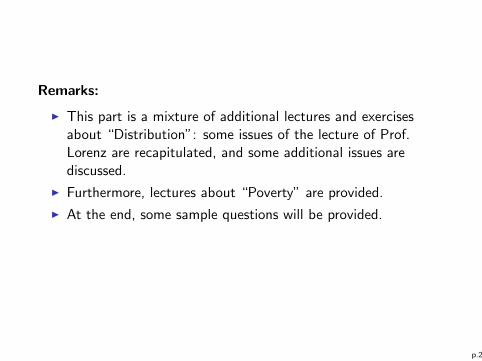
Remarks:
I This part is a mixture of additional lectures and exercisesabout “Distribution”: some issues of the lecture of Prof.Lorenz are recapitulated, and some additional issues arediscussed.
I Furthermore, lectures about “Poverty” are provided.
I At the end, some sample questions will be provided.
p.2
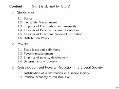
Content: (ch. 3 is planned for future)
1. Distribution
1.1 Basics1.2 Inequaility Measurement1.3 Empirics of Distribution and Inequality1.4 Theories of Personal Income Distribution1.5 Theories of Functional Income Distribution1.6 Distribution Policy
2. Poverty
2.1 Basic ideas and definitions2.2 Poverty measurement2.3 Empirics of poverty development2.4 Determinants of poverty
3. Redistribution and Poverty Reduction in a Liberal Society
3.1 Justification of redistribution in a liberal society?3.2 Political economy of redistribution
p.3
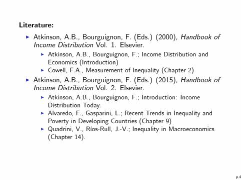
Literature:
I Atkinson, A.B., Bourguignon, F. (Eds.) (2000), Handbook ofIncome Distribution Vol. 1. Elsevier.
I Atkinson, A.B., Bourguignon, F.; Income Distribution andEconomics (Introduction)
I Cowell, F.A., Measurement of Inequality (Chapter 2)
I Atkinson, A.B., Bourguignon, F. (Eds.) (2015), Handbook ofIncome Distribution Vol. 2. Elsevier.
I Atkinson, A.B., Bourguignon, F.; Introduction: IncomeDistribution Today.
I Alvaredo, F., Gasparini, L.; Recent Trends in Inequality andPoverty in Developing Countries (Chapter 9)
I Quadrini, V., Rıos-Rull, J.-V.; Inequality in Macroeconomics(Chapter 14).
p.4
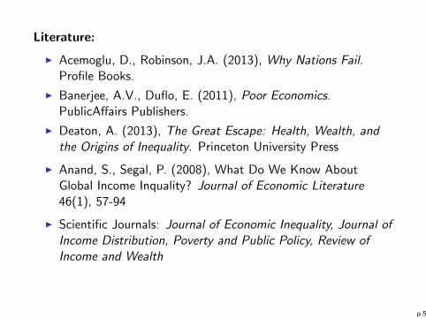
Literature:
I Acemoglu, D., Robinson, J.A. (2013), Why Nations Fail.Profile Books.
I Banerjee, A.V., Duflo, E. (2011), Poor Economics.PublicAffairs Publishers.
I Deaton, A. (2013), The Great Escape: Health, Wealth, andthe Origins of Inequality. Princeton University Press
I Anand, S., Segal, P. (2008), What Do We Know AboutGlobal Income Inquality? Journal of Economic Literature46(1), 57-94
I Scientific Journals: Journal of Economic Inequality, Journal ofIncome Distribution, Poverty and Public Policy, Review ofIncome and Wealth
p.5
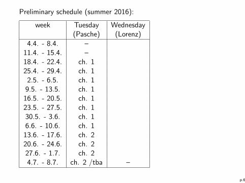
Preliminary schedule (summer 2016):
week Tuesday Wednesday(Pasche) (Lorenz)
4.4. - 8.4. –11.4. - 15.4. –18.4. - 22.4. ch. 125.4. - 29.4. ch. 1
2.5. - 6.5. ch. 19.5. - 13.5. ch. 1
16.5. - 20.5. ch. 123.5. - 27.5. ch. 130.5. - 3.6. ch. 16.6. - 10.6. ch. 1
13.6. - 17.6. ch. 220.6. - 24.6. ch. 227.6. - 1.7. ch. 24.7. - 8.7. ch. 2 /tba –
p.6
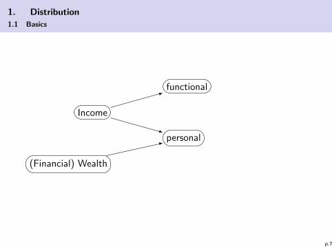
1. Distribution
1.1 Basics
Income
(Financial) Wealth
functional
personal
p.7
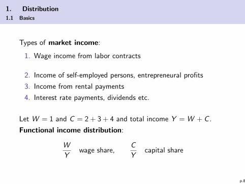
1. Distribution
1.1 Basics
Types of market income:
1. Wage income from labor contracts
2. Income of self-employed persons, entrepreneural profits
3. Income from rental payments
4. Interest rate payments, dividends etc.
Let W = 1 and C = 2 + 3 + 4 and total income Y = W + C .
Functional income distribution:
W
Ywage share,
C
Ycapital share
p.8
1. Distribution
1.1 Basics
Effective or disposable income:
= Market income - Income taxes + Transfers
(income after redistributional policies)
I Primary functional distribution: wage share of marketincome
I Secondary functional distribution: wage share of disposableincome
p.9
1. Distribution
1.1 Basics
Problem:
I If the wage share declines (capital share increases), does thismean that workers are “loosing”?
⇒ Not necessarily because it could also be the case that morepeople become self-employed.
I We have to adjust the wage ratio for the effct of changingshare of dependend workers.
⇒ Adjusted Wage (Labour) Share
I Moreover: Functional distrintion doesn’t say much aboutpersonal distribution.
p.10
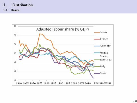
1. Distribution
1.1 Basics
p.11
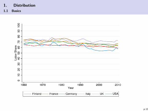
1. Distribution
1.1 Basics
p.12
1. Distribution
1.1 Basics
I Functional income distribution and personal incomedistribution are theoretically independent from each other.
I However, capital is very inequally distributed. Hence anincreasing capital income will ceteris paribus affect both,functional and personal distribution.
I We will come back to functional income distribution in thecontext of distribution theory.
p.13
1. Distribution
1.1 Basics
(Financial) Wealth:
I Financial assets: money, bonds, equity capital shares, lifeinsurance claims
I Real estate (ground, buildings)
I Physical assets (cars, jewels, ....)
I Pension claims
I etc.....
⇒ Not easy to measure!
Income = flow variable, wealth = stock variable
p.14
1. Distribution
1.1 Basics
Problems:
I What could be justified to be part of wealth?
I What is the “value” of these assets (e.g. mark-to-marketapproach for houses and stock shares)?
I What about liabilities/debt?
Net Wealth = Wealth - Liabilities
Net Wealth could be negative!
p.15
1. Distribution
1.2 Inequality Measurement
What do we mean by “inequaility”?
Agenda:
I Preliminaries, properties of inequality measures
I Distributions, variance coefficient
I Lorenz curve
I Gini coefficient
I Theil index
I Atkinson index
p.16
1. Distribution
1.2 Inequality Measurement
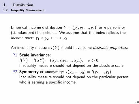
Empirical income distribution Y = (y1, y2, ..., yn) for n persons or(standardized) households. We assume that the index reflects theincome oder : y1 < y2 < ... < yn.
An inequality measure I (Y ) should have some desirable properties:
P1 Scale invariance:I (Y ) = I (αY ) = (αy1, αy2, ..., αyn), α > 0.Inequality measure should not depend on the absolute scale.
P2 Symmetry or anonymity: I (y1, ..., yn) = I (yn, ..., y1)Inequality measure should not depend on the particular personwho is earning a specific income.
p.17
1. Distribution
1.2 Inequality Measurement
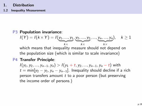
P3 Population invariance:I (Y ) = I (k×Y ) = I (y1, ..., y1︸ ︷︷ ︸
k×
, y2, ..., y2︸ ︷︷ ︸k×
, ..., yn, ..., yn︸ ︷︷ ︸k×
), k ≥ 1
which means that inequality measure should not depend onthe population size (which is similar to scale invariance)
P4 Transfer Principle:I (y1, y2, ..., yn−1, yn) > I (y1 + t, y2, ..., yn−1, yn − t) witht = min[y2 − y1, yn − yn−1]. Inequality should decline if a richperson transfers amount t to a poor person (but preservingthe income order of persons.)
p.18
1. Distribution
1.2 Inequality Measurement
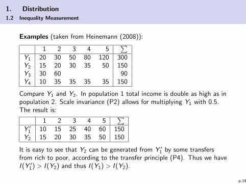
Examples (taken from Heinemann (2008)):
1 2 3 4 5∑
Y1 20 30 50 80 120 300Y2 15 20 30 35 50 150Y3 30 60 90Y4 10 35 35 35 35 150
Compare Y1 and Y2. In population 1 total income is double as high as inpopulation 2. Scale invariance (P2) allows for multiplying Y1 with 0.5.The result is:
1 2 3 4 5∑
Y ′1 10 15 25 40 60 150
Y2 15 20 30 35 50 150
It is easy to see that Y2 can be generated from Y ′1 by some transfers
from rich to poor, according to the transfer principle (P4). Thus we haveI (Y ′
1) > I (Y2) and thus I (Y1) > I (Y2).
p.19
1. Distribution
1.2 Inequality Measurement
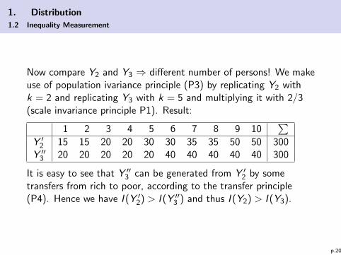
Now compare Y2 and Y3 ⇒ different number of persons! We makeuse of population ivariance principle (P3) by replicating Y2 withk = 2 and replicating Y3 with k = 5 and multiplying it with 2/3(scale invariance principle P1). Result:
1 2 3 4 5 6 7 8 9 10∑
Y ′2 15 15 20 20 30 30 35 35 50 50 300Y ′′3 20 20 20 20 20 40 40 40 40 40 300
It is easy to see that Y ′′3 can be generated from Y ′2 by sometransfers from rich to poor, according to the transfer principle(P4). Hence we have I (Y ′2) > I (Y ′′3 ) and thus I (Y2) > I (Y3).
p.20
1. Distribution
1.2 Inequality Measurement
I However, in most empirically relevant cases the principlesP1-P4 do not allow a clear characterization of inequality!
⇒ Inequality measures have to add more criteria – and thereforemore normative value judgements!
p.21
1. Distribution
1.2 Inequality Measurement
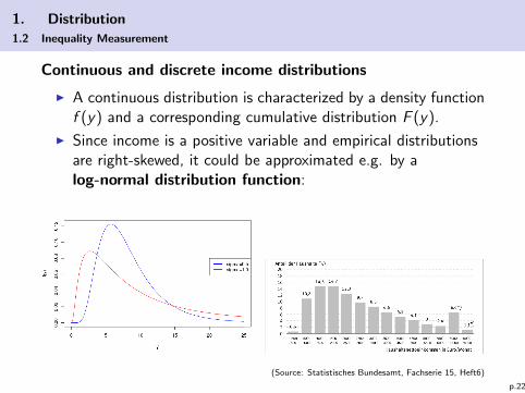
Continuous and discrete income distributions
I A continuous distribution is characterized by a density functionf (y) and a corresponding cumulative distribution F (y).
I Since income is a positive variable and empirical distributionsare right-skewed, it could be approximated e.g. by alog-normal distribution function:
(Source: Statistisches Bundesamt, Fachserie 15, Heft6)
p.22
1. Distribution
1.2 Inequality Measurement
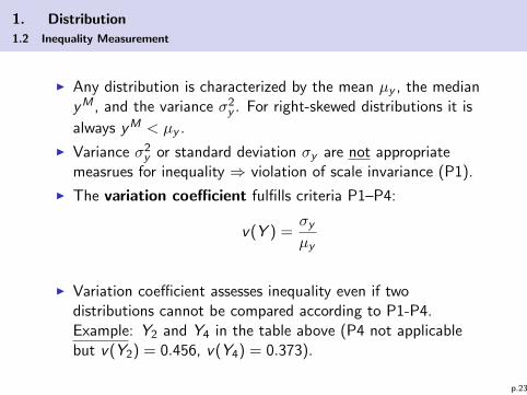
I Any distribution is characterized by the mean µy , the medianyM , and the variance σ2
y . For right-skewed distributions it is
always yM < µy .
I Variance σ2y or standard deviation σy are not appropriate
measrues for inequality ⇒ violation of scale invariance (P1).
I The variation coefficient fulfills criteria P1–P4:
v(Y ) =σyµy
I Variation coefficient assesses inequality even if twodistributions cannot be compared according to P1-P4.Example: Y2 and Y4 in the table above (P4 not applicablebut v(Y2) = 0.456, v(Y4) = 0.373).
p.23
1. Distribution
1.2 Inequality Measurement
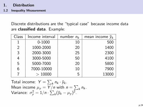
Discrete distributions are the “typical case” because income dataare classified data. Example:
Class Income interval number nk mean income yk1 0-1000 10 5002 1000-2000 20 14003 2000-3000 25 23004 3000-5000 50 41005 5000-7000 20 58006 7000-10000 10 79007 > 10000 5 13000
Total income: Y =∑
k nk · yk .Mean income µy = Y /n with n =
∑k nk .
Variance: σ2y = 1/n ·
∑k(yk − µy )2.
p.24
1. Distribution
1.2 Inequality Measurement
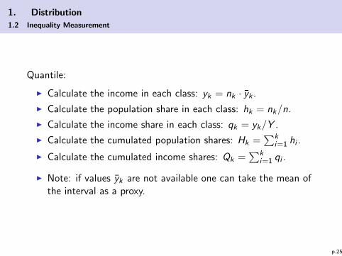
Quantile:
I Calculate the income in each class: yk = nk · yk .
I Calculate the population share in each class: hk = nk/n.
I Calculate the income share in each class: qk = yk/Y .
I Calculate the cumulated population shares: Hk =∑k
i=1 hi .
I Calculate the cumulated income shares: Qk =∑k
i=1 qi .
I Note: if values yk are not available one can take the mean ofthe interval as a proxy.
p.25
1. Distribution
1.2 Inequality Measurement
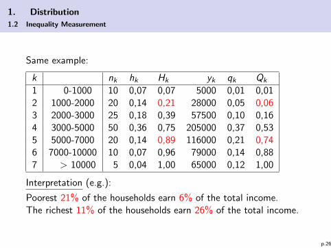
Same example:
k nk hk Hk yk qk Qk
1 0-1000 10 0,07 0,07 5000 0,01 0,012 1000-2000 20 0,14 0,21 28000 0,05 0,063 2000-3000 25 0,18 0,39 57500 0,10 0,164 3000-5000 50 0,36 0,75 205000 0,37 0,535 5000-7000 20 0,14 0,89 116000 0,21 0,746 7000-10000 10 0,07 0,96 79000 0,14 0,887 > 10000 5 0,04 1,00 65000 0,12 1,00
Interpretation (e.g.):
Poorest 21% of the households earn 6% of the total income.The richest 11% of the households earn 26% of the total income.
p.26
1. Distribution
1.2 Inequality Measurement
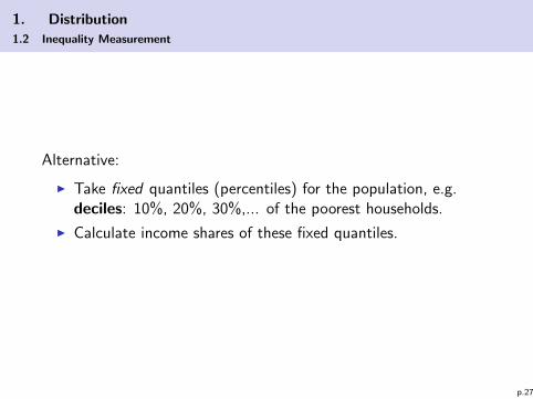
Alternative:
I Take fixed quantiles (percentiles) for the population, e.g.deciles: 10%, 20%, 30%,... of the poorest households.
I Calculate income shares of these fixed quantiles.
p.27
1. Distribution
1.2 Inequality Measurement
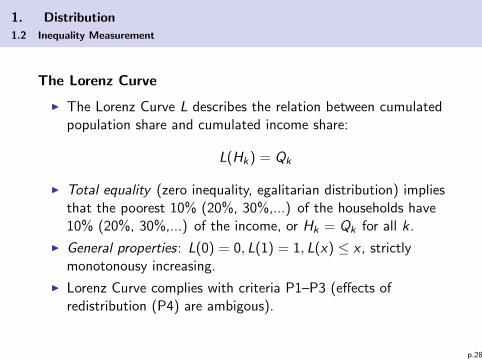
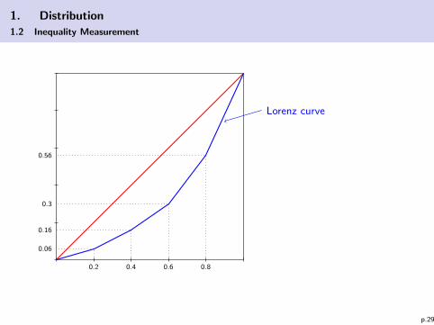
The Lorenz Curve
I The Lorenz Curve L describes the relation between cumulatedpopulation share and cumulated income share:
L(Hk) = Qk
I Total equality (zero inequality, egalitarian distribution) impliesthat the poorest 10% (20%, 30%,...) of the households have10% (20%, 30%,...) of the income, or Hk = Qk for all k .
I General properties: L(0) = 0, L(1) = 1, L(x) ≤ x , strictlymonotonousy increasing.
I Lorenz Curve complies with criteria P1–P3 (effects ofredistribution (P4) are ambigous).
p.28
1. Distribution
1.2 Inequality Measurement
0.2
0.06
0.4
0.16
0.6
0.3
0.8
0.56
Lorenz curve
p.29
1. Distribution
1.2 Inequality Measurement
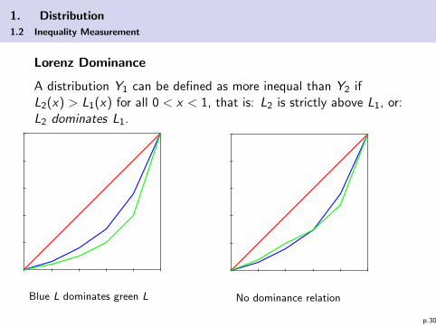
Lorenz Dominance
A distribution Y1 can be defined as more inequal than Y2 ifL2(x) > L1(x) for all 0 < x < 1, that is: L2 is strictly above L1, or:L2 dominates L1.
Blue L dominates green L No dominance relation
p.30
1. Distribution
1.2 Inequality Measurement
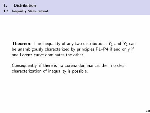
Theorem: The inequality of any two distributions Y1 and Y2 canbe unambigously characterized by principles P1–P4 if and only ifone Lorenz curve dominates the other.
Consequently, if there is no Lorenz dominance, then no clearcharacterization of inequality is possible.
p.31
1. Distribution
1.2 Inequality Measurement
What can be measured with Lorenz Curves (examples):
I Market income distribution
I Effective/disposable income distribution
I Taxes (round about 10% richest households pay 40% ofincome taxes, richest 20% pay 70% of the taxes)
I (Financial) Wealth: Significantly larger inequality in wealthdistribution than in income distribution.
p.32
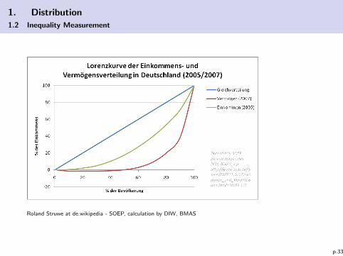
1. Distribution
1.2 Inequality Measurement
Roland Struwe at de.wikipedia - SOEP, calculation by DIW, BMAS
p.33
1. Distribution
1.2 Inequality Measurement
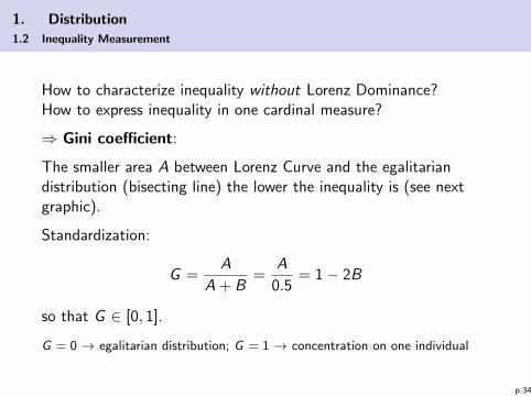
How to characterize inequality without Lorenz Dominance?How to express inequality in one cardinal measure?
⇒ Gini coefficient:
The smaller area A between Lorenz Curve and the egalitariandistribution (bisecting line) the lower the inequality is (see nextgraphic).
Standardization:
G =A
A + B=
A
0.5= 1− 2B
so that G ∈ [0, 1].
G = 0 → egalitarian distribution; G = 1 → concentration on one individual
p.34
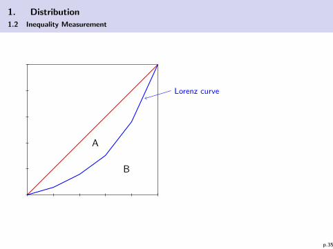
1. Distribution
1.2 Inequality Measurement
Lorenz curve
A
B
p.35
1. Distribution
1.2 Inequality Measurement
For individual (non-classified) income data like in the table above theexact formula is
G =1
2n2µy
n∑i=1
n∑j=1
|yi − yj |
(Normalized sum of all absolute income differences.)
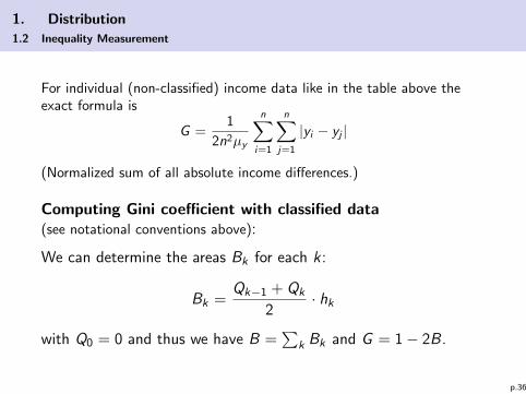
Computing Gini coefficient with classified data(see notational conventions above):
We can determine the areas Bk for each k :
Bk =Qk−1 + Qk
2· hk
with Q0 = 0 and thus we have B =∑
k Bk and G = 1− 2B.
p.36
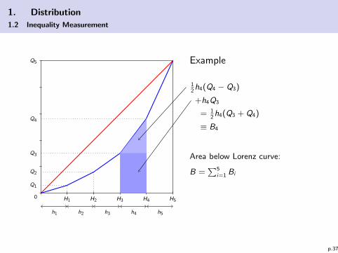
1. Distribution
1.2 Inequality Measurement
H1
Q1
H2
Q2
H3
Q3
H4
Q4
H5
Q5
0
h1 h2 h3 h4 h5
Example
12h4(Q4 − Q3)
+h4Q3
= 12h4(Q3 + Q4)
≡ B4
Area below Lorenz curve:
B =∑5
i=1 Bi
p.37
1. Distribution
1.2 Inequality Measurement
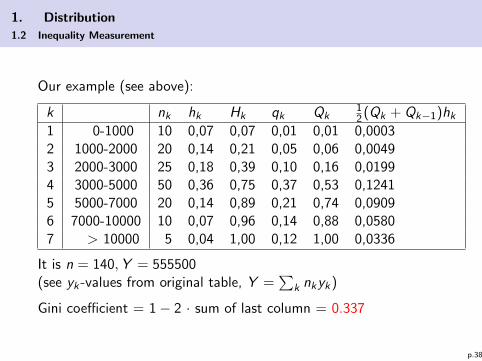
Our example (see above):
k nk hk Hk qk Qk12 (Qk + Qk−1)hk
1 0-1000 10 0,07 0,07 0,01 0,01 0,00032 1000-2000 20 0,14 0,21 0,05 0,06 0,00493 2000-3000 25 0,18 0,39 0,10 0,16 0,01994 3000-5000 50 0,36 0,75 0,37 0,53 0,12415 5000-7000 20 0,14 0,89 0,21 0,74 0,09096 7000-10000 10 0,07 0,96 0,14 0,88 0,05807 > 10000 5 0,04 1,00 0,12 1,00 0,0336
It is n = 140,Y = 555500(see yk -values from original table, Y =
∑k nkyk)
Gini coefficient = 1− 2 · sum of last column = 0.337
p.38
1. Distribution
1.2 Inequality Measurement
Note:
I Gini coefficient is a widely used inequality measure inempirical studies and in the political debate.
I Like the variation coefficient, the Gini coefficient comparesinequalities for distributions even if criteria P1–P4 areinsufficient for a characterization = where there is no Lorenzdominance!
I Obviously, a distribution Y1 which is Lorenz dominating Y2
must have a lower Gini coefficient. The reverse claim is nottrue.
p.39
1. Distribution
1.2 Inequality Measurement
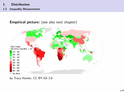
Empirical picture: (see also next chapter)
by Tracy Hunter, CC BY-SA 3.0
p.40
1. Distribution
1.2 Inequality Measurement
A constant or even declining Gini coefficient is often misinterpretedin the way that the “gap between rich and poor does notbecome larger”.
However, by comparing two distributions with the same Ginicoefficient we cannot say much about the “gap between rich andpoor”. A larger gap might be consistent with constant or evenlower Gini coefficient!
⇒ Need for indices measuring polarization.
p.41
1. Distribution
1.2 Inequality Measurement
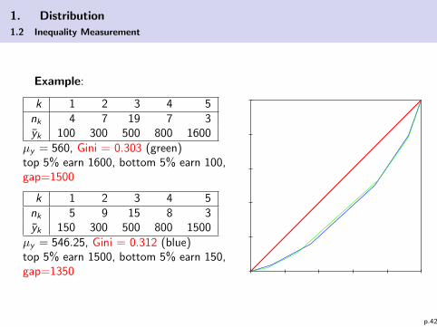
Example:
k 1 2 3 4 5nk 4 7 19 7 3yk 100 300 500 800 1600
µy = 560, Gini = 0.303 (green)top 5% earn 1600, bottom 5% earn 100,gap=1500
k 1 2 3 4 5nk 5 9 15 8 3yk 150 300 500 800 1500
µy = 546.25, Gini = 0.312 (blue)top 5% earn 1500, bottom 5% earn 150,gap=1350
p.42
1. Distribution
1.2 Inequality Measurement
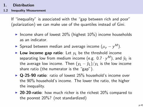
If “inequality” is associated with the “gap between rich and poor”(polarization) we can make use of the quantiles instead of Gini.
I Income share of lowest 20% (highest 10%) income householdsas an indicator.
I Spread between median and average income (µy − yM).
I Low income gap ratio: Let yL be the threshold incomeseparating low from medium income (e.g. 0.7 · yM), and yL isthe average low income. Then (yL − yL)/yL is the low incomeshare ratio (the numerator is the “gap”).
I Q-25-90 ratio: ratio of lowest 25% household’s income overthe 90% household’s income. The lower the ratio, the higherthe inequality.
I 20-20-ratio: how much richer is the richest 20% compared tothe poorest 20%? (not standardized)
p.43
1. Distribution
1.2 Inequality Measurement
Further remarks on the Gini coefficient:
I The coefficient is not (easily) decomposable!
⇒ Investigating subclasses of a distribution, e.g. differencesbetween regions, sectors, sexes etc. ⇒ requires inequalitymeasurement within groups and between groups.
⇒ The Gini coefficient of total populaion cannot be decomposede.g. as a (weighted) convex combination of the Ginicoefficients of the particular subgroups ⇒ not very favorableproperty!
I There exist some methods for decomposing Gini coefficientsbut they require knowledge which is typically not available,e.g. the full distribution.
p.44
1. Distribution
1.2 Inequality Measurement
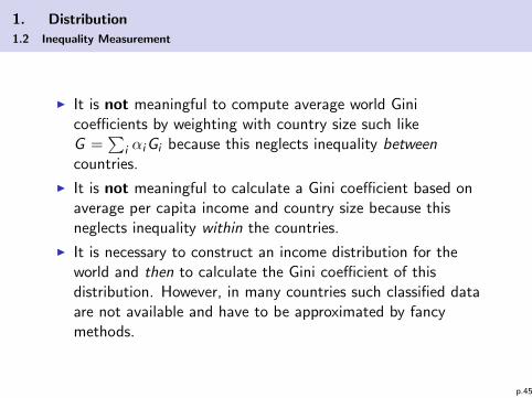
I It is not meaningful to compute average world Ginicoefficients by weighting with country size such likeG =
∑i αiGi because this neglects inequality between
countries.
I It is not meaningful to calculate a Gini coefficient based onaverage per capita income and country size because thisneglects inequality within the countries.
I It is necessary to construct an income distribution for theworld and then to calculate the Gini coefficient of thisdistribution. However, in many countries such classified dataare not available and have to be approximated by fancymethods.
p.45
1. Distribution
1.2 Inequality Measurement
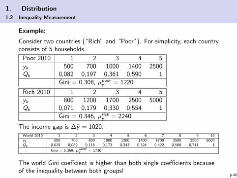
Example:
Consider two countries (“Rich” and “Poor”). For simplicity, each countryconsists of 5 households.
Poor 2010 1 2 3 4 5yk 500 700 1000 1400 2500Qk 0,082 0,197 0,361 0,590 1
Gini = 0.308, µpoory = 1220
Rich 2010 1 2 3 4 5yk 800 1200 1700 2500 5000Qk 0,071 0,179 0,330 0,554 1
Gini = 0.346, µrichy = 2240
The income gap is ∆y = 1020.World 2010 1 2 3 4 5 6 7 8 9 10yk 500 700 800 1000 1200 1400 1700 2500 2500 5000Qk 0,029 0,069 0,116 0,173 0,243 0,324 0,422 0,566 0,711 1
Gini = 0.369, µworldy = 1730
The world Gini coeffcient is higher than both single coefficients becauseof the inequality between both groups!
p.46
1. Distribution
1.2 Inequality Measurement
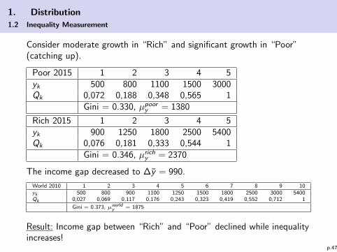
Consider moderate growth in “Rich” and significant growth in “Poor”(catching up).
Poor 2015 1 2 3 4 5yk 500 800 1100 1500 3000Qk 0,072 0,188 0,348 0,565 1
Gini = 0.330, µpoory = 1380
Rich 2015 1 2 3 4 5yk 900 1250 1800 2500 5400Qk 0,076 0,181 0,333 0,544 1
Gini = 0.346, µrichy = 2370
The income gap decreased to ∆y = 990.
World 2010 1 2 3 4 5 6 7 8 9 10yk 500 800 900 1100 1250 1500 1800 2500 3000 5400Qk 0,027 0,069 0,117 0,176 0,243 0,323 0,419 0,552 0,712 1
Gini = 0.373, µworldy = 1875
Result: Income gap between “Rich” and “Poor” declined while inequalityincreases!
p.47
1. Distribution
1.2 Inequality Measurement
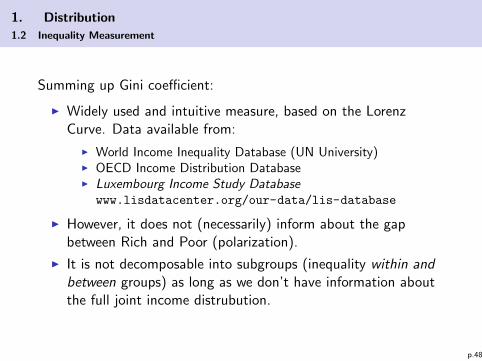
Summing up Gini coefficient:
I Widely used and intuitive measure, based on the LorenzCurve. Data available from:
I World Income Inequality Database (UN University)I OECD Income Distribution DatabaseI Luxembourg Income Study Database
www.lisdatacenter.org/our-data/lis-database
I However, it does not (necessarily) inform about the gapbetween Rich and Poor (polarization).
I It is not decomposable into subgroups (inequality within andbetween groups) as long as we don’t have information aboutthe full joint income distrubution.
p.48
1. Distribution
1.2 Inequality Measurement
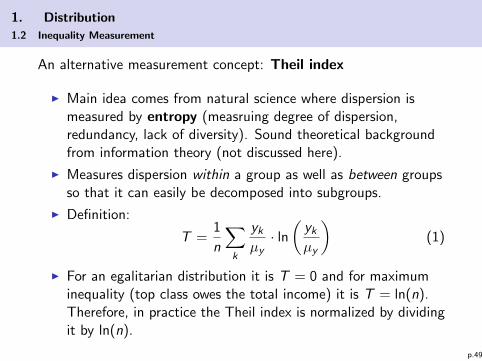
An alternative measurement concept: Theil index
I Main idea comes from natural science where dispersion ismeasured by entropy (measruing degree of dispersion,redundancy, lack of diversity). Sound theoretical backgroundfrom information theory (not discussed here).
I Measures dispersion within a group as well as between groupsso that it can easily be decomposed into subgroups.
I Definition:
T =1
n
∑k
ykµy· ln(
ykµy
)(1)
I For an egalitarian distribution it is T = 0 and for maximuminequality (top class owes the total income) it is T = ln(n).Therefore, in practice the Theil index is normalized by dividingit by ln(n).
p.49
1. Distribution
1.2 Inequality Measurement
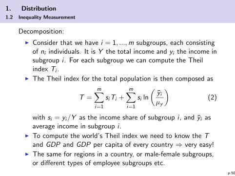
Decomposition:
I Consider that we have i = 1, ...,m subgroups, each consistingof ni individuals. It is Y the total income and yi the income insubgroup i . For each subgroup we can compute the Theilindex Ti .
I The Theil index for the total population is then composed as
T =m∑i=1
siTi +m∑i=1
si ln
(yiµy
)(2)
with si = yi/Y as the income share of subgroup i , and yi asaverage income in subgroup i .
I To compute the world’s Theil index we need to know the Tand GDP and GDP per capita of every country ⇒ very easy!
I The same for regions in a country, or male-female subgroups,or different types of employee subgroups etc.
p.50
1. Distribution
1.2 Inequality Measurement
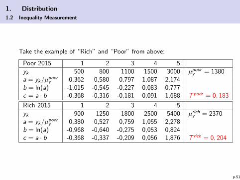
Take the example of “Rich” and “Poor” from above:
Poor 2015 1 2 3 4 5yk 500 800 1100 1500 3000 µpoor
y = 1380a = yk/µ
poory 0,362 0,580 0,797 1,087 2,174
b = ln(a) -1,015 -0,545 -0,227 0,083 0,777c = a · b -0,368 -0,316 -0,181 0,091 1,688 T poor = 0, 183
Rich 2015 1 2 3 4 5yk 900 1250 1800 2500 5400 µrich
y = 2370a = yk/µ
poory 0,380 0,527 0,759 1,055 2,278
b = ln(a) -0,968 -0,640 -0,275 0,053 0,824c = a · b -0,368 -0,337 -0,209 0,056 1,876 T rich = 0, 204
p.51
1. Distribution
1.2 Inequality Measurement
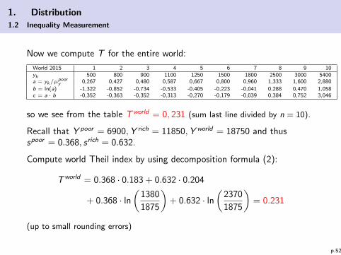
Now we compute T for the entire world:
World 2015 1 2 3 4 5 6 7 8 9 10yk 500 800 900 1100 1250 1500 1800 2500 3000 5400a = yk/µ
poory 0,267 0,427 0,480 0,587 0,667 0,800 0,960 1,333 1,600 2,880
b = ln(a) -1,322 -0,852 -0,734 -0,533 -0,405 -0,223 -0,041 0,288 0,470 1,058c = a · b -0,352 -0,363 -0,352 -0,313 -0,270 -0,179 -0,039 0,384 0,752 3,046
so we see from the table Tworld = 0, 231 (sum last line divided by n = 10).
Recall that Y poor = 6900,Y rich = 11850,Y world = 18750 and thusspoor = 0.368, s rich = 0.632.
Compute world Theil index by using decomposition formula (2):
Tworld = 0.368 · 0.183 + 0.632 · 0.204
+ 0.368 · ln(
1380
1875
)+ 0.632 · ln
(2370
1875
)= 0.231
(up to small rounding errors)
p.52
1. Distribution
1.2 Inequality Measurement
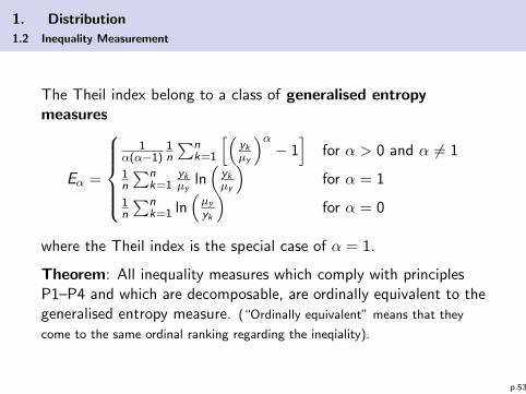
The Theil index belong to a class of generalised entropymeasures
Eα =
1
α(α−1)1n
∑nk=1
[(ykµy
)α− 1]
for α > 0 and α 6= 1
1n
∑nk=1
ykµy
ln(
ykµy
)for α = 1
1n
∑nk=1 ln
(µyyk
)for α = 0
where the Theil index is the special case of α = 1.
Theorem: All inequality measures which comply with principlesP1–P4 and which are decomposable, are ordinally equivalent to thegeneralised entropy measure. (“Ordinally equivalent” means that they
come to the same ordinal ranking regarding the ineqiality).
p.53
1. Distribution
1.2 Inequality Measurement
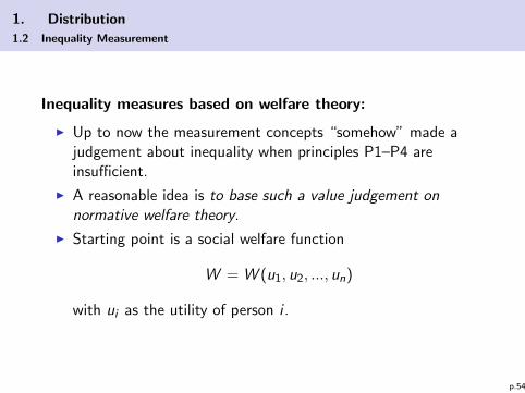
Inequality measures based on welfare theory:
I Up to now the measurement concepts “somehow” made ajudgement about inequality when principles P1–P4 areinsufficient.
I A reasonable idea is to base such a value judgement onnormative welfare theory.
I Starting point is a social welfare function
W = W (u1, u2, ..., un)
with ui as the utility of person i .
p.54
1. Distribution
1.2 Inequality Measurement
Important:
I From Arrow’s Impossibility Theorem we know that it is notpossible to derive a collective preference order (and thus:collective utility function) consistently from individualpreferences. Axioms of utility theory do not allow anycomparison of individual utility. Thus, these axioms do notprovide a basis for a socially optimal “compromise”.
⇒ Therefore, a welfare function W makes the implicit valuejudgement that we can compare individual utilities!
p.55
1. Distribution
1.2 Inequality Measurement
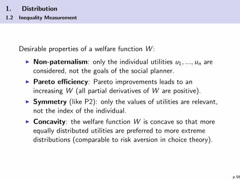
Desirable properties of a welfare function W :
I Non-paternalism: only the individual utilities u1, ..., un areconsidered, not the goals of the social planner.
I Pareto efficiency: Pareto improvements leads to anincreasing W (all partial derivatives of W are positive).
I Symmetry (like P2): only the values of utilities are relevant,not the index of the individual.
I Concavity: the welfare function W is concave so that moreequally distributed utilities are preferred to more extremedistributions (comparable to risk aversion in choice theory).
p.56
1. Distribution
1.2 Inequality Measurement
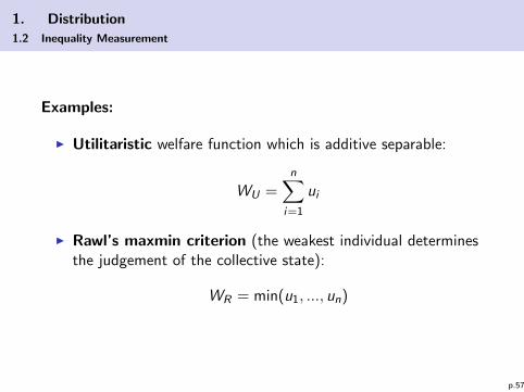
Examples:
I Utilitaristic welfare function which is additive separable:
WU =n∑
i=1
ui
I Rawl’s maxmin criterion (the weakest individual determinesthe judgement of the collective state):
WR = min(u1, ..., un)
p.57
1. Distribution
1.2 Inequality Measurement
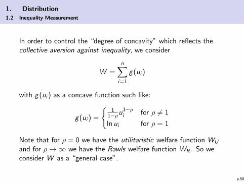
In order to control the “degree of concavity” which reflects thecollective aversion against inequality, we consider
W =n∑
i=1
g(ui )
with g(ui ) as a concave function such like:
g(ui ) =
{1
1−ρu1−ρi for ρ 6= 1
ln ui for ρ = 1
Note that for ρ = 0 we have the utilitaristic welfare function WU
and for ρ→∞ we have the Rawls welfare function WR . So weconsider W as a “general case”.
p.58
1. Distribution
1.2 Inequality Measurement
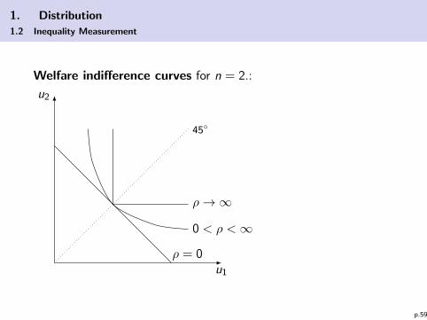
Welfare indifference curves for n = 2.:
u2
u1
45◦
ρ = 0
ρ→∞
0 < ρ <∞
p.59
1. Distribution
1.2 Inequality Measurement
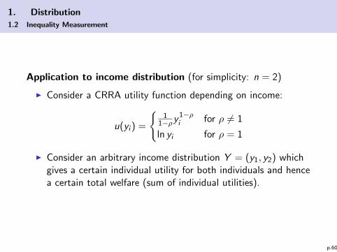
Application to income distribution (for simplicity: n = 2)
I Consider a CRRA utility function depending on income:
u(yi ) =
{1
1−ρy 1−ρi for ρ 6= 1
ln yi for ρ = 1
I Consider an arbitrary income distribution Y = (y1, y2) whichgives a certain individual utility for both individuals and hencea certain total welfare (sum of individual utilities).
p.60
1. Distribution
1.2 Inequality Measurement
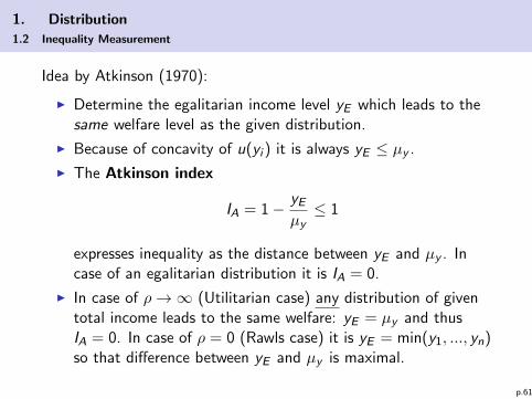
Idea by Atkinson (1970):
I Determine the egalitarian income level yE which leads to thesame welfare level as the given distribution.
I Because of concavity of u(yi ) it is always yE ≤ µy .
I The Atkinson index
IA = 1− yEµy≤ 1
expresses inequality as the distance between yE and µy . Incase of an egalitarian distribution it is IA = 0.
I In case of ρ→∞ (Utilitarian case) any distribution of giventotal income leads to the same welfare: yE = µy and thusIA = 0. In case of ρ = 0 (Rawls case) it is yE = min(y1, ..., yn)so that difference between yE and µy is maximal.
p.61
1. Distribution
1.2 Inequality Measurement
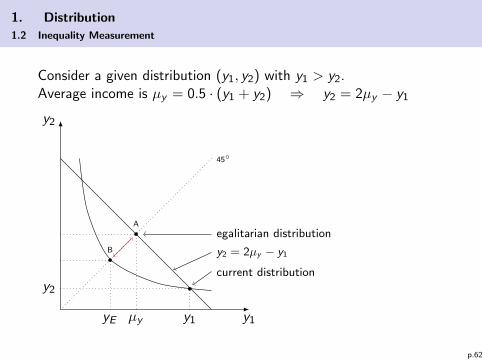
Consider a given distribution (y1, y2) with y1 > y2.Average income is µy = 0.5 · (y1 + y2) ⇒ y2 = 2µy − y1
y2
y1
y2
y1
current distribution
y2 = 2µy − y1
45◦
A
egalitarian distribution
µy
B
yE
p.62
1. Distribution
1.2 Inequality Measurement
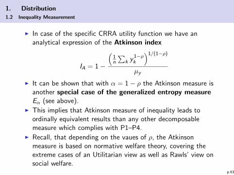
I In case of the specific CRRA utility function we have ananalytical expression of the Atkinson index
IA = 1−
(1n
∑k y 1−ρ
k
)1/(1−ρ)
µy
I It can be shown that with α = 1− ρ the Atkinson measure isanother special case of the generalized entropy measureEα (see above).
I This implies that Atkinson measure of inequality leads toordinally equivalent results than any other decomposablemeasure which complies with P1–P4.
I Recall, that depending on the vaues of ρ, the Atkinsonmeasure is based on normative welfare theory, covering theextreme cases of an Utilitarian view as well as Rawls’ view onsocial welfare.
p.63
1. Distribution
1.2 Inequality Measurement
Final remarks:
I Measuring the degree of inequality doesn’t imply anythingabout the desriability of a more egalitarian distribution or thesocial acceptance of inequality. How much inequality is“too much” depends on normative judgements.
I Inequality might be more acceptable if there is a high incomemobility (individual chance to enter higher quantiles indistribution), independent from determinants like sex, incomeof parents, education, skin color etc.
I Recall that many inequality measures (e.g. Gini) do not referto the gap between “rich” and “poor”. Measuring thisdisparity (polarization) require other (ad hoc) measurementconcepts.
p.64
1. Distribution
1.3 Empirics of Distribution and Inequality
Agenda:
a) Increasing inequality in Germany?
b) European and global trends
c) Links between inequality and growth
p.65
1. Distribution
1.3 Empirics of Distribution and Inequality
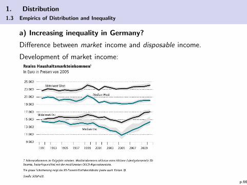
a) Increasing inequality in Germany?
Difference between market income and disposable income.
Development of market income:
p.66
1. Distribution
1.3 Empirics of Distribution and Inequality
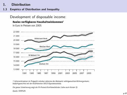
Development of disposable income:
p.67
1. Distribution
1.3 Empirics of Distribution and Inequality
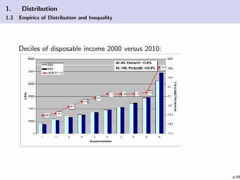
Deciles of disposable income 2000 versus 2010:
p.68
1. Distribution
1.3 Empirics of Distribution and Inequality
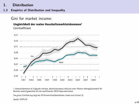
Gini for market income:
p.69
1. Distribution
1.3 Empirics of Distribution and Inequality
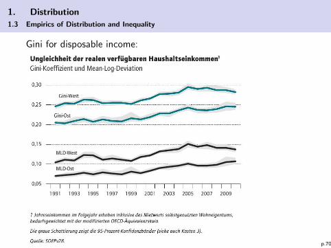
Gini for disposable income:
p.70
1. Distribution
1.3 Empirics of Distribution and Inequality
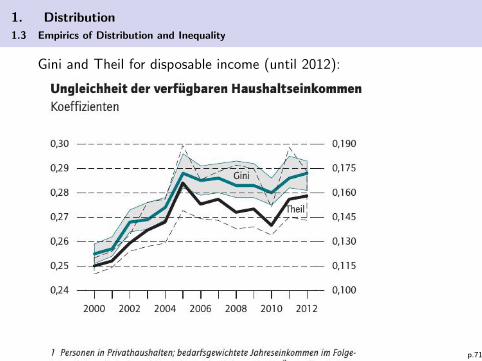
Gini and Theil for disposable income (until 2012):
p.71
1. Distribution
1.3 Empirics of Distribution and Inequality
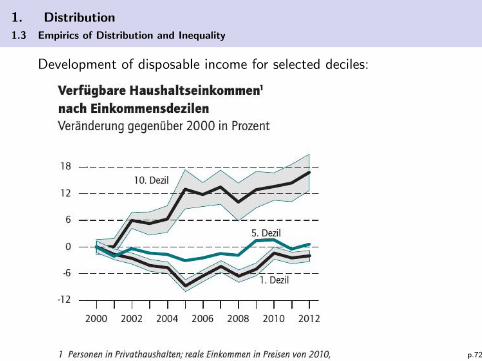
Development of disposable income for selected deciles:
p.72
1. Distribution
1.3 Empirics of Distribution and Inequality
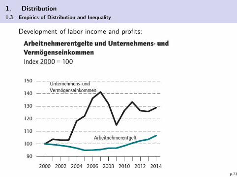
Development of labor income and profits:
p.73
1. Distribution
1.3 Empirics of Distribution and Inequality
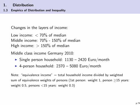
Changes in the layers of income:
Low income: < 70% of medianMiddle income: 70% - 150% of medianHigh income: > 150% of median
Middle class income Germany 2010:
I Single person household: 1130 – 2420 Euro/month
I 4-person household: 2370 – 5080 Euro/month
Note: “equivalence income” = total household income divided by weighted
sum of equivalence weights of persons (1st person: weight 1, person ≥15 years:
weight 0.5, persons <15 years: weight 0.3)
p.74
1. Distribution
1.3 Empirics of Distribution and Inequality
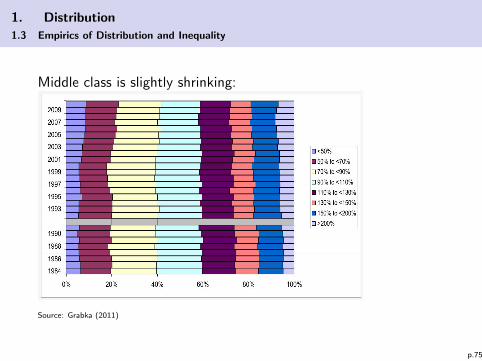
Middle class is slightly shrinking:
Source: Grabka (2011)
p.75
1. Distribution
1.3 Empirics of Distribution and Inequality
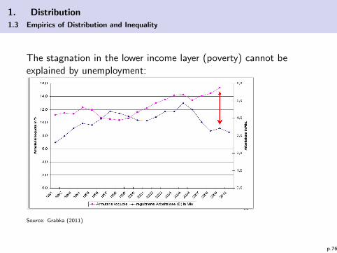
The stagnation in the lower income layer (poverty) cannot beexplained by unemployment:
Source: Grabka (2011)
p.76
1. Distribution
1.3 Empirics of Distribution and Inequality
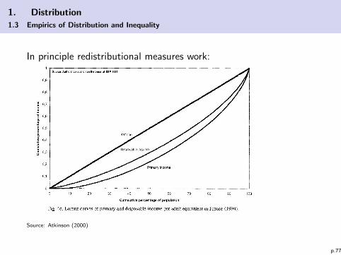
In principle redistributional measures work:
Source: Atkinson (2000)
p.77
1. Distribution
1.3 Empirics of Distribution and Inequality
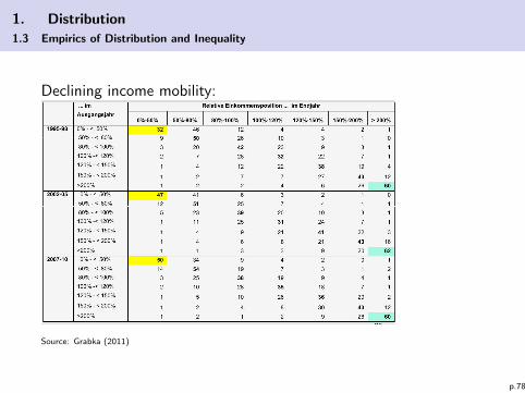
Declining income mobility:
Source: Grabka (2011)
p.78
1. Distribution
1.3 Empirics of Distribution and Inequality
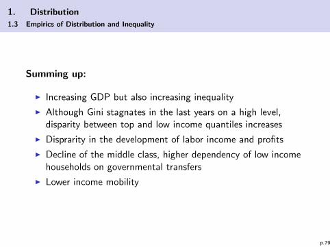
Summing up:
I Increasing GDP but also increasing inequality
I Although Gini stagnates in the last years on a high level,disparity between top and low income quantiles increases
I Disprarity in the development of labor income and profits
I Decline of the middle class, higher dependency of low incomehouseholds on governmental transfers
I Lower income mobility
p.79
1. Distribution
1.3 Empirics of Distribution and Inequality
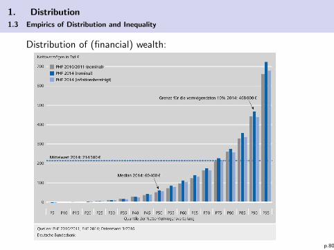
Distribution of (financial) wealth:
p.80
1. Distribution
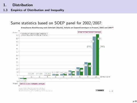
1.3 Empirics of Distribution and Inequality
Same statistics based on SOEP panel for 2002/2007:
p.81
1. Distribution
1.3 Empirics of Distribution and Inequality
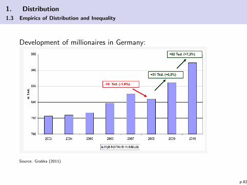
Development of millionaires in Germany:
Source: Grabka (2011)
p.82
1. Distribution
1.3 Empirics of Distribution and Inequality
Summing up (Bundesbank study 2016):
I Gross and net wealth increased
I Very inequal distribution (Gini = 0.76, nearly constant in lastyears)
I Median increased but lower 40% quantile has slightly declinedwealth.
I Most massive increase in top 1%
Stylized picture for income and wealth in the last 5-10 years:
I More or less stable Gini coefficients, but...
I ... increasing disparity (polarization),
I lower third of society seem to be decoupled from positiveaverage development.
p.83
1. Distribution
1.3 Empirics of Distribution and Inequality
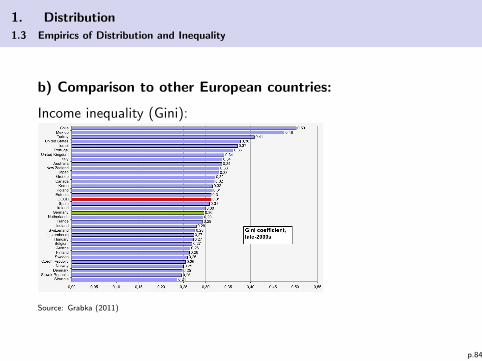
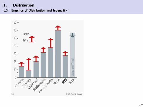
b) Comparison to other European countries:
Income inequality (Gini):
Source: Grabka (2011)
p.84
1. Distribution
1.3 Empirics of Distribution and Inequality
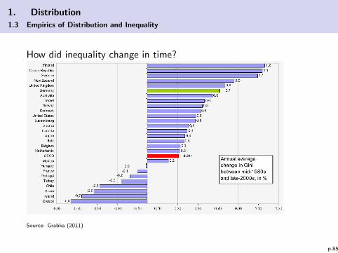
How did inequality change in time?
Source: Grabka (2011)
p.85
1. Distribution
1.3 Empirics of Distribution and Inequality
p.86

1. Distribution
1.3 Empirics of Distribution and Inequality
Income growth in quantiles:
(taken from Bauermann (2015))
p.87
1. Distribution
1.3 Empirics of Distribution and Inequality
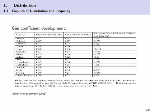
Gini coefficient development:
(taken from Bauermann (2015))
p.88
1. Distribution
1.3 Empirics of Distribution and Inequality
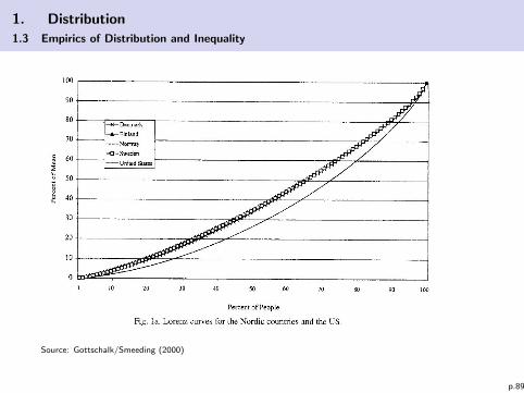
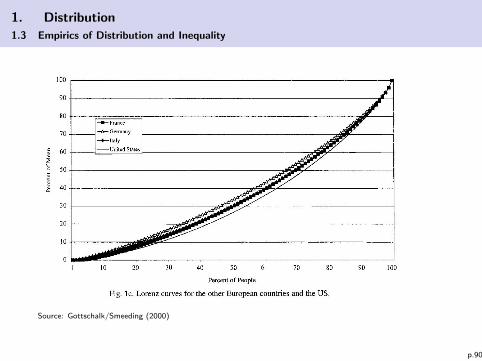
Source: Gottschalk/Smeeding (2000)
p.89
1. Distribution
1.3 Empirics of Distribution and Inequality
Source: Gottschalk/Smeeding (2000)
p.90
1. Distribution
1.3 Empirics of Distribution and Inequality
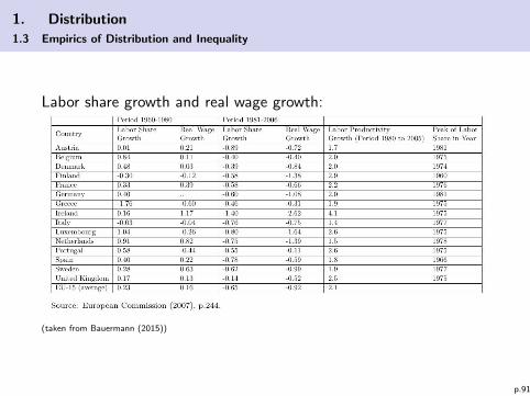
Labor share growth and real wage growth:
(taken from Bauermann (2015))
p.91
1. Distribution
1.3 Empirics of Distribution and Inequality
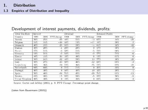
Development of interest payments, dividends, profits:
(taken from Bauermann (2015))
p.92
1. Distribution
1.3 Empirics of Distribution and Inequality
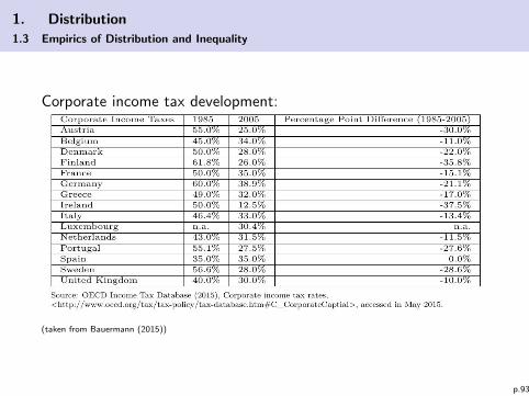
Corporate income tax development:
(taken from Bauermann (2015))
p.93
1. Distribution
1.3 Empirics of Distribution and Inequality
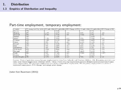
Part-time employment, temporary employment:
(taken from Bauermann (2015))
p.94
1. Distribution
1.3 Empirics of Distribution and Inequality
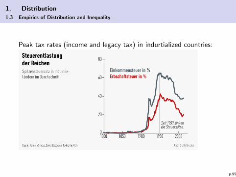
Peak tax rates (income and legacy tax) in indurtialized countries:
p.95
1. Distribution
1.3 Empirics of Distribution and Inequality
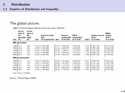
The global picture:
Source: Anand/Segal (2008)
p.96
1. Distribution
1.3 Empirics of Distribution and Inequality
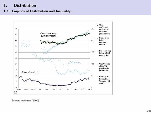
Source: Atkinson (2000)
p.97
1. Distribution
1.3 Empirics of Distribution and Inequality
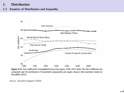
Source: Alvaredo/Gasparini (2015)
p.98
1. Distribution
1.3 Empirics of Distribution and Inequality
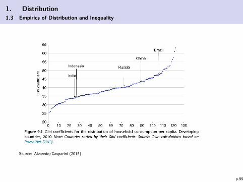
Source: Alvaredo/Gasparini (2015)
p.99
1. Distribution
1.3 Empirics of Distribution and Inequality
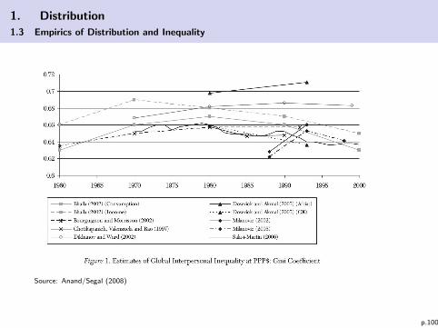
Source: Anand/Segal (2008)
p.100
1. Distribution
1.3 Empirics of Distribution and Inequality
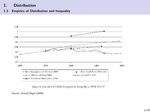
Source: Anand/Segal (2008)
p.101
1. Distribution
1.3 Empirics of Distribution and Inequality
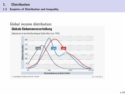
Global income distribution:
p.102
1. Distribution
1.3 Empirics of Distribution and Inequality
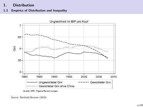
Source: Berthold/Brunner (2010)
p.103
1. Distribution
1.3 Empirics of Distribution and Inequality
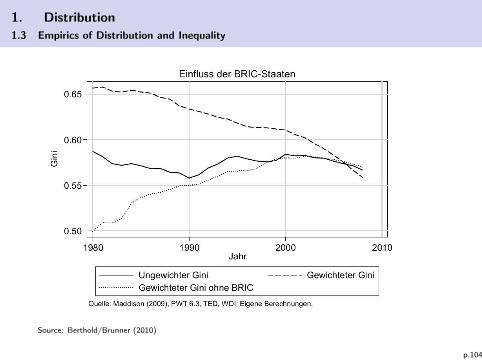
Source: Berthold/Brunner (2010)
p.104
1. Distribution
1.3 Empirics of Distribution and Inequality
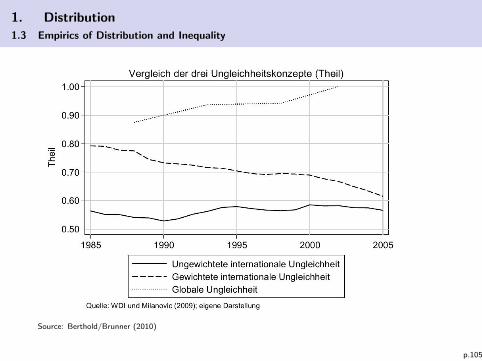
Source: Berthold/Brunner (2010)
p.105
1. Distribution
1.3 Empirics of Distribution and Inequality
Comments on global inequality:
I Picture not so clear, depends on calcuation of PPP adjusted incomeand databse and used index.
I Problem of within-country and between-country inequality (seediscussion about decomposability of Theil versus Gini).
I BRIC countries: growing prosperity in middle class and thusincreasing GDP per capita leads to lower between-country Ginicoefficients.
I However, Gini and Theil don’t provide information aboutpolarization.
I Global inequality in financial wealth increased drastically.
I Links between wealth and income distribution, role of lessredistributional efforts for top deciles.
I OECD/European countries: increased within-country inequality inlast decades, stagnating income inequality in last 5-10 years, butslightly increasing polarization, especially for wealth.
p.106
1. Distribution
1.3 Empirics of Distribution and Inequality
c) Inequality and Growth
Counterveiling positions:
I Is inequality good or bad for growth?
I Does groeth foster or dampen inequality?
⇒ Most empirical studies consider the first causality.
I No effect or positive relationship: Li and Zou (1998), Barro(2000)
I Negative relationship: Persson and Tabellini (1994), Galor andZeira (1993)
p.107
1. Distribution
1.3 Empirics of Distribution and Inequality
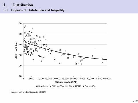
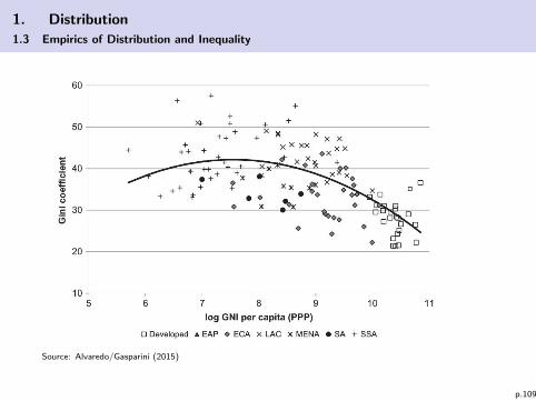
Source: Alvaredo/Gasparini (2015)
p.108
1. Distribution
1.3 Empirics of Distribution and Inequality
Source: Alvaredo/Gasparini (2015)
p.109
1. Distribution
1.3 Empirics of Distribution and Inequality
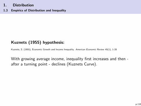
Kuznets (1955) hypothesis:
Kuznets, S. (1955), Economic Growth and Income Inequality. American Economic Review 45(1), 1-28
With growing average income, inequality first increases and then -after a turning point - declines (Kuznets Curve).
p.110
1. Distribution
1.3 Empirics of Distribution and Inequality
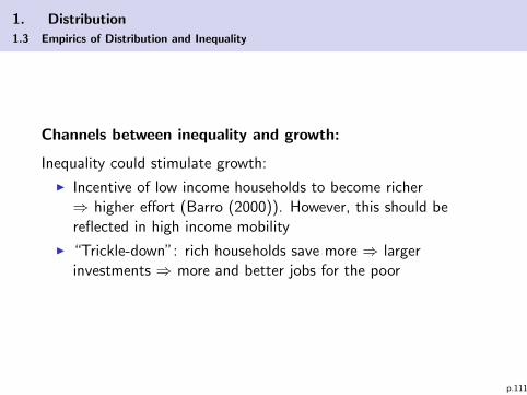
Channels between inequality and growth:
Inequality could stimulate growth:
I Incentive of low income households to become richer⇒ higher effort (Barro (2000)). However, this should bereflected in high income mobility
I “Trickle-down”: rich households save more ⇒ largerinvestments ⇒ more and better jobs for the poor
p.111
1. Distribution
1.3 Empirics of Distribution and Inequality
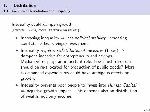
Inequality could dampen growth(Perotti (1995), more literature on reuest):
I Increasing inequality ⇒ less political stability, increasingconflicts ⇒ less savings/investment
I Inequality requires redistributional measures (taxes) ⇒dampens incentive for entrepreneurs and savings.Median voter plays an important role: how much resourcesshould be re-allocated for production of public goods? Moretax-financed expenditures could have ambigous effects ongrowth.
I Inequality prevents poor people to invest into Human Capital⇒ negative growth impact. This depends also on distributionof wealth, not only income.
p.112
1. Distribution
1.3 Empirics of Distribution and Inequality
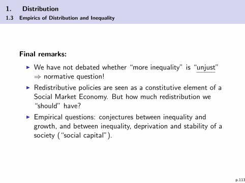
Final remarks:
I We have not debated whether “more inequality” is “unjust”⇒ normative question!
I Redistributive policies are seen as a constitutive element of aSocial Market Economy. But how much redistribution we“should” have?
I Empirical questions: conjectures between inequality andgrowth, and between inequality, deprivation and stability of asociety (“social capital”).
p.113
1. Distribution
1.4 Theories of Personal Income Distribution
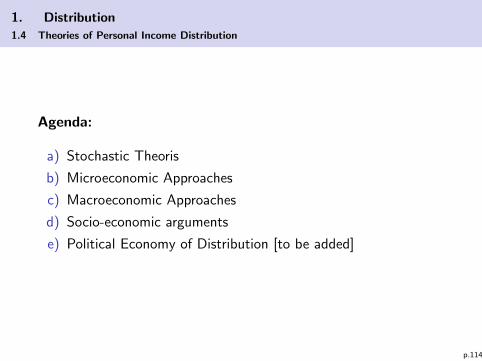
Agenda:
a) Stochastic Theoris
b) Microeconomic Approaches
c) Macroeconomic Approaches
d) Socio-economic arguments
e) Political Economy of Distribution [to be added]
p.114
1. Distribution
1.4 Theories of Personal Income Distribution
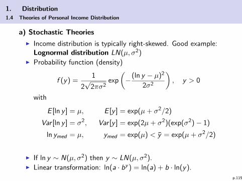
a) Stochastic Theories
I Income distribution is typically right-skewed. Good example:Lognormal distribution LN(µ, σ2)
I Probability function (density)
f (y) =1
2√
2πσ2exp
(−(ln y − µ)2
2σ2
), y > 0
with
E [ln y ] = µ, E [y ] = exp(µ+ σ2/2)
Var [ln y ] = σ2, Var [y ] = exp(2µ+ σ2)(exp(σ2)− 1)
ln ymed = µ, ymed = exp(µ) < y = exp(µ+ σ2/2)
I If ln y ∼ N(µ, σ2) then y ∼ LN(µ, σ2).I Linear transformation: ln(a · by ) = ln(a) + b · ln(y).
p.115
1. Distribution
1.4 Theories of Personal Income Distribution
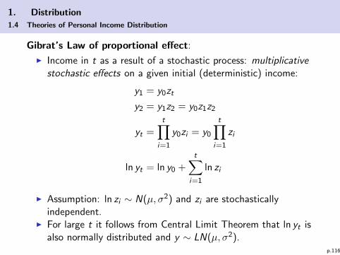
Gibrat’s Law of proportional effect:
I Income in t as a result of a stochastic process: multiplicativestochastic effects on a given initial (deterministic) income:
y1 = y0zt
y2 = y1z2 = y0z1z2
yt =t∏
i=1
y0zi = y0
t∏i=1
zi
ln yt = ln y0 +t∑
i=1
ln zi
I Assumption: ln zi ∼ N(µ, σ2) and zi are stochasticallyindependent.
I For large t it follows from Central Limit Theorem that ln yt isalso normally distributed and y ∼ LN(µ, σ2).
p.116
1. Distribution
1.4 Theories of Personal Income Distribution
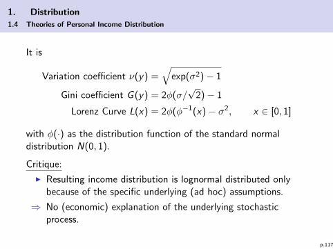
It is
Variation coefficient ν(y) =√
exp(σ2)− 1
Gini coefficient G (y) = 2φ(σ/√
2)− 1
Lorenz Curve L(x) = 2φ(φ−1(x)− σ2, x ∈ [0, 1]
with φ(·) as the distribution function of the standard normaldistribution N(0, 1).
Critique:
I Resulting income distribution is lognormal distributed onlybecause of the specific underlying (ad hoc) assumptions.
⇒ No (economic) explanation of the underlying stochasticprocess.
p.117
1. Distribution
1.4 Theories of Personal Income Distribution
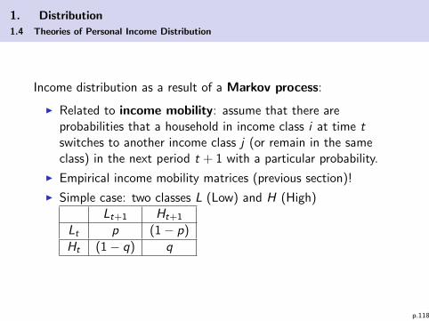
Income distribution as a result of a Markov process:
I Related to income mobility: assume that there areprobabilities that a household in income class i at time tswitches to another income class j (or remain in the sameclass) in the next period t + 1 with a particular probability.
I Empirical income mobility matrices (previous section)!
I Simple case: two classes L (Low) and H (High)Lt+1 Ht+1
Lt p (1− p)
Ht (1− q) q
p.118
1. Distribution
1.4 Theories of Personal Income Distribution
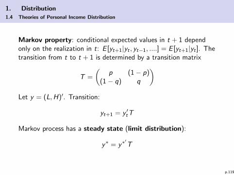
Markov property: conditional expected values in t + 1 dependonly on the realization in t: E [yt+1|yt , yt−1, ....] = E [yt+1|yt ]. Thetransition from t to t + 1 is determined by a transition matrix
T =
(p (1− p)
(1− q) q
)Let y = (L,H)′. Transition:
yt+1 = y ′tT
Markov process has a steady state (limit distribution):
y∗ = y∗′T
p.119
1. Distribution
1.4 Theories of Personal Income Distribution
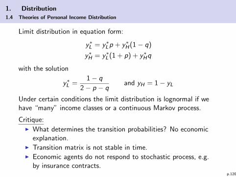
Limit distribution in equation form:
y∗L = y∗Lp + y∗H(1− q)
y∗H = y∗L (1 + p) + y∗Hq
with the solution
y∗L =1− q
2− p − qand yH = 1− yL
Under certain conditions the limit distribution is lognormal if wehave “many” income classes or a continuous Markov process.
Critique:I What determines the transition probabilities? No economic
explanation.I Transition matrix is not stable in time.I Economic agents do not respond to stochastic process, e.g.
by insurance contracts.p.120
1. Distribution
1.4 Theories of Personal Income Distribution
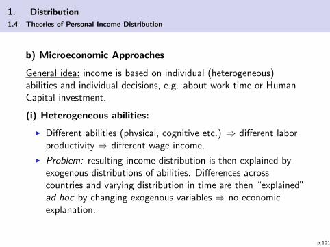
b) Microeconomic Approaches
General idea: income is based on individual (heterogeneous)abilities and individual decisions, e.g. about work time or HumanCapital investment.
(i) Heterogeneous abilities:
I Different abilities (physical, cognitive etc.) ⇒ different laborproductivity ⇒ different wage income.
I Problem: resulting income distribution is then explained byexogenous distributions of abilities. Differences acrosscountries and varying distribution in time are then “explained”ad hoc by changing exogenous variables ⇒ no economicexplanation.
p.121
1. Distribution
1.4 Theories of Personal Income Distribution
I Alternative: abilities depend also on “learning-by-doing”.These effects might differ across sectors and work type, anddepend on experience/age, but are not an intentional result ofdecisions.
(ii) Individual decisions:
I Different decisions regarding time allocation (work – leisure)
I Different investments into Human Capital
p.122
1. Distribution
1.4 Theories of Personal Income Distribution
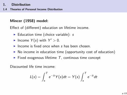
Mincer (1958) model:
Effect of (different) education on lifetime income.
I Education time (choice variable): s
I Income Y (s) with Y ′ > 0.
I Income is fixed once when s has been chosen.
I No income in education time (opportunity cost of education)
I Fixed exogenous lifetime T , continous time concept
Discounted life time income:
L(s) =
∫ T
se−itY (s)dt = Y (s)
∫ T
se−itdt
p.123
1. Distribution
1.4 Theories of Personal Income Distribution
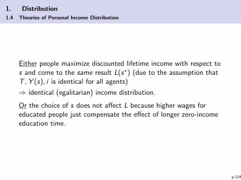
Either people maximize discounted lifetime income with respect tos and come to the same result L(s∗) (due to the assumption thatT ,Y (s), i is identical for all agents)
⇒ identical (egalitarian) income distribution.
Or the choice of s does not affect L because higher wages foreducated people just compensate the effect of longer zero-incomeeducation time.
p.124
1. Distribution
1.4 Theories of Personal Income Distribution
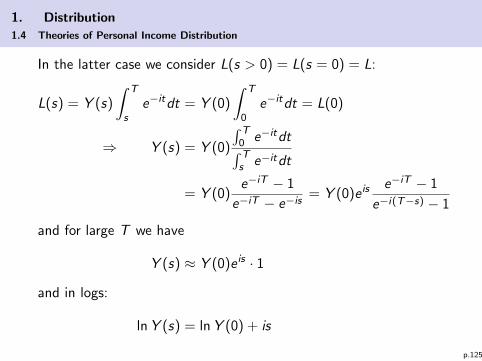
In the latter case we consider L(s > 0) = L(s = 0) = L:
L(s) = Y (s)
∫ T
se−itdt = Y (0)
∫ T
0e−itdt = L(0)
⇒ Y (s) = Y (0)
∫ T0 e−itdt∫ Ts e−itdt
= Y (0)e−iT − 1
e−iT − e−is= Y (0)e is
e−iT − 1
e−i(T−s) − 1
and for large T we have
Y (s) ≈ Y (0)e is · 1
and in logs:
ln Y (s) = ln Y (0) + is
p.125
1. Distribution
1.4 Theories of Personal Income Distribution
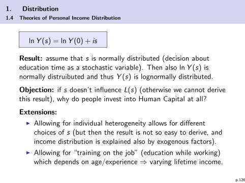
ln Y (s) = ln Y (0) + is
Result: assume that s is normally distributed (decision abouteducation time as a stochastic variable). Then also ln Y (s) isnormally distruibuted and thus Y (s) is lognormally distributed.
Objection: if s doesn’t influence L(s) (otherwise we cannot derivethis result), why do people invest into Human Capital at all?
Extensions:
I Allowing for individual heterogeneity allows for differentchoices of s (but then the result is not so easy to derive, andincome distribution is explained also by exogenous factors).
I Allowing for “training on the job” (education while working)which depends on age/experience ⇒ varying lifetime income.
p.126
1. Distribution
1.4 Theories of Personal Income Distribution
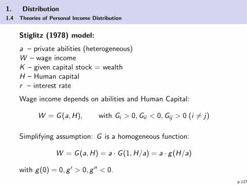
Stiglitz (1978) model:
a – private abilities (heterogeneous)W – wage incomeK – given capital stock = wealthH – Human capitalr – interest rate
Wage income depends on abilities and Human Capital:
W = G (a,H), with Gi > 0,Gii < 0,Gij > 0 (i 6= j)
Simplifying assumption: G is a homogeneous function:
W = G (a,H) = a · G (1,H/a) = a · g(H/a)
with g(0) = 0, g ′ > 0, g ′′ < 0.
p.127
1. Distribution
1.4 Theories of Personal Income Distribution
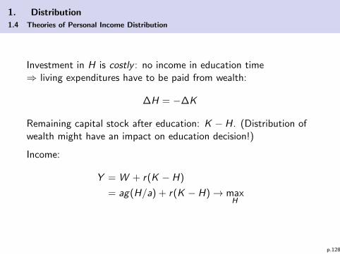
Investment in H is costly : no income in education time⇒ living expenditures have to be paid from wealth:
∆H = −∆K
Remaining capital stock after education: K − H. (Distribution ofwealth might have an impact on education decision!)
Income:
Y = W + r(K − H)
= ag(H/a) + r(K − H)→ maxH
p.128
1. Distribution
1.4 Theories of Personal Income Distribution
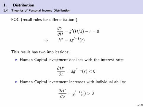
FOC (recall rules for differentiation!):
dY
dH= g ′(H/a)− r = 0
⇒ H∗ = ag′−1(r)
This result has two implications:
I Human Capital investment declines with the interest rate:
∂H∗
∂r= ag
′′−1(r) < 0
I Human Capital investment increases with individual ability:
∂H∗
∂a= g
′−1(r) > 0
p.129
1. Distribution
1.4 Theories of Personal Income Distribution
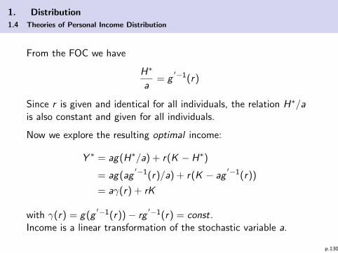
From the FOC we have
H∗
a= g
′−1(r)
Since r is given and identical for all individuals, the relation H∗/ais also constant and given for all individuals.
Now we explore the resulting optimal income:
Y ∗ = ag(H∗/a) + r(K − H∗)
= ag(ag′−1(r)/a) + r(K − ag
′−1(r))
= aγ(r) + rK
with γ(r) = g(g′−1(r))− rg
′−1(r) = const.Income is a linear transformation of the stochastic variable a.
p.130
1. Distribution
1.4 Theories of Personal Income Distribution
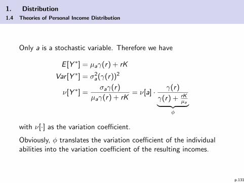
Only a is a stochastic variable. Therefore we have
E [Y ∗] = µaγ(r) + rK
Var [Y ∗] = σ2a(γ(r))2
ν[Y ∗] =σaγ(r)
µaγ(r) + rK= ν[a] · γ(r)
γ(r) + rKµa︸ ︷︷ ︸
φ
with ν[·] as the variation coefficient.
Obviously, φ translates the variation coefficient of the individualabilities into the variation coefficient of the resulting incomes.
p.131
1. Distribution
1.4 Theories of Personal Income Distribution
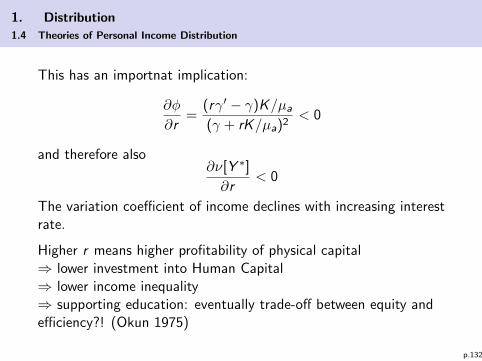
This has an importnat implication:
∂φ
∂r=
(rγ′ − γ)K/µa(γ + rK/µa)2
< 0
and therefore also∂ν[Y ∗]
∂r< 0
The variation coefficient of income declines with increasing interestrate.
Higher r means higher profitability of physical capital⇒ lower investment into Human Capital⇒ lower income inequality⇒ supporting education: eventually trade-off between equity andefficiency?! (Okun 1975)
p.132
1. Distribution
1.4 Theories of Personal Income Distribution
Extensions:
I Allowing for a mix of (costly) Human Capital investment andlearning-by-doing and heterogeneous individual abilities.
I Leads to both, income distribution for all individuals andvarying individual income over lifetime.
I Considering decisions about financial wealth (e.g. savingrates)
Some remarks:
I Most models consider competitive markets. Determination ofwages and interest rates also depends on market power.
I Most models are partial equilibrium models, e.g. neglectingthat Human Capital investment affect capital productivity.
I For studying the interaction of distribution and growth (andeventually technical progress), macroeconomic approaches areused.
p.133
1. Distribution
1.4 Theories of Personal Income Distribution
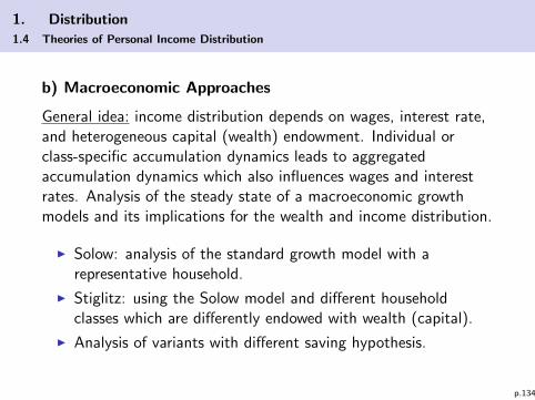
b) Macroeconomic Approaches
General idea: income distribution depends on wages, interest rate,and heterogeneous capital (wealth) endowment. Individual orclass-specific accumulation dynamics leads to aggregatedaccumulation dynamics which also influences wages and interestrates. Analysis of the steady state of a macroeconomic growthmodels and its implications for the wealth and income distribution.
I Solow: analysis of the standard growth model with arepresentative household.
I Stiglitz: using the Solow model and different householdclasses which are differently endowed with wealth (capital).
I Analysis of variants with different saving hypothesis.
p.134
1. Distribution
1.4 Theories of Personal Income Distribution
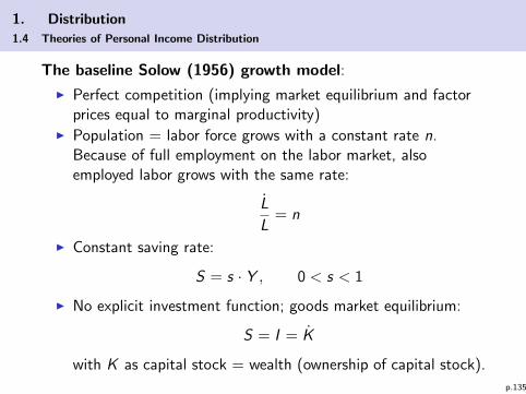
The baseline Solow (1956) growth model:
I Perfect competition (implying market equilibrium and factorprices equal to marginal productivity)
I Population = labor force grows with a constant rate n.Because of full employment on the labor market, alsoemployed labor grows with the same rate:
L
L= n
I Constant saving rate:
S = s · Y , 0 < s < 1
I No explicit investment function; goods market equilibrium:
S = I = K
with K as capital stock = wealth (ownership of capital stock).
p.135
1. Distribution
1.4 Theories of Personal Income Distribution
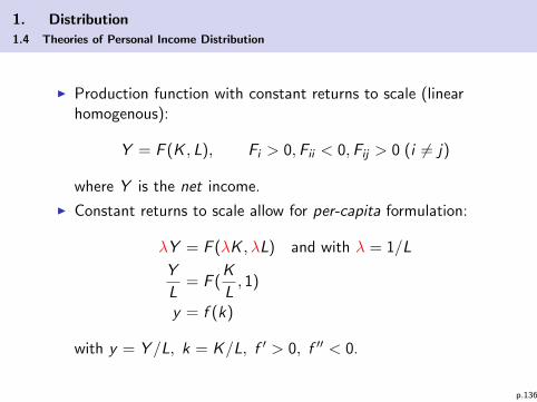
I Production function with constant returns to scale (linearhomogenous):
Y = F (K , L), Fi > 0,Fii < 0,Fij > 0 (i 6= j)
where Y is the net income.
I Constant returns to scale allow for per-capita formulation:
λY = F (λK , λL) and with λ = 1/L
Y
L= F (
K
L, 1)
y = f (k)
with y = Y /L, k = K/L, f ′ > 0, f ′′ < 0.
p.136
1. Distribution
1.4 Theories of Personal Income Distribution
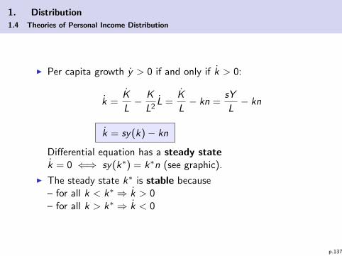
I Per capita growth y > 0 if and only if k > 0:
k =K
L− K
L2L =
K
L− kn =
sY
L− kn
k = sy(k)− kn
Differential equation has a steady statek = 0 ⇐⇒ sy(k∗) = k∗n (see graphic).
I The steady state k∗ is stable because– for all k < k∗ ⇒ k > 0– for all k > k∗ ⇒ k < 0
p.137
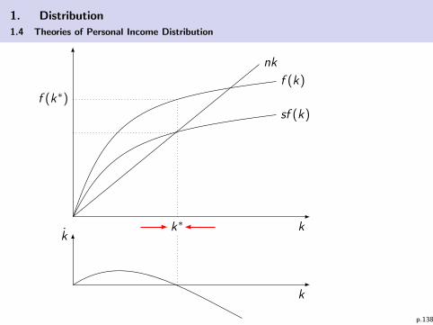
1. Distribution
1.4 Theories of Personal Income Distribution
k
f (k)
sf (k)
nk
k∗
f (k∗)
k
k
p.138
1. Distribution
1.4 Theories of Personal Income Distribution
I Recall that per capita income is y = w + rk.
I Factors are paid according to their marginal productivity:
r = r(k) = f ′(k)
w = w(k) = f (k)− r(k)k
(Note that Euler theorem holds true: output is completely allocated
to the input factors, no residual profits.)
I Important to note: marginal productivities depend on thecapital intensity k ⇒ wages and interest rates depends on theaccumulation dynamics!
p.139
1. Distribution
1.4 Theories of Personal Income Distribution
Stiglitz (1969) variant of the basline growth model:
I Assume m classes i = 1, ...,m
I Reproduction rate n is identical in all classes.
I Labor endowment Li .
I Capital (wealth) endowment Ki is heterogeneous.
⇒ Class-specific per capita income: yi = w + rki
p.140
1. Distribution
1.4 Theories of Personal Income Distribution
I Class-specific accumulation dynamics:
ki =Ki
Li− nki
= sy(ki )− nki
= s(w(k) + r(k)ki )− nki
= sw(k)− [n − sr(k)]ki
I For a class-specific steady-state ki = 0 we have
k∗i =sw(k)
n − sr(k)
where the r.h.s. depends only on macro variables. Thus thesteady-state is the same for all classes!
I This implies that there is a convergence to an egalitariandistribution of wealth and thus income – independent fromthe initial distribution!
p.141
1. Distribution
1.4 Theories of Personal Income Distribution
I Aggregation in the Stiglitz-Solow model:
k =∑i
Ki
L=∑i
Ki
Li
Li
L=∑i
kiai
with∑
i ai = 1 (class shares).I This can be applied to the aggregated dynamics:
k =∑i
ai ki
=∑i
ai [sy(ki )− nki ]
= s∑i
aiy(ki )− n∑i
aiki
= sy(k)− nk
which was proven to have a stable steady state.p.142
1. Distribution
1.4 Theories of Personal Income Distribution
Implication: micro dynamic for each class is stable:
I Making use of r(k) = f ′(k) and w(k) = f (k)− f ′(k)k theclass-specific dynamic is
ki = s(w + rki )− nki
= s(f (k)− f ′(k)k + f ′(k)ki )− nki
= sf (k) + sf ′(k)[ki − k]︸ ︷︷ ︸A
− nki︸︷︷︸B
I Consider the steady state k∗ and split up the r.h.s. into A andB for a graphical analysis of ki (see graphic).
I The graphical analysis shows that– for ki < k∗ ⇒ ki > 0– for ki > k∗ ⇒ ki < 0
p.143
1. Distribution
1.4 Theories of Personal Income Distribution
k , ki
sf (k)
nk (or nki )
k∗
sf (k∗) + sf ′(k∗)[ki − k∗]
kAi kB
i
ki = sf (k∗) + sf ′(k∗)[ki − k∗]− nki
p.144

1. Distribution
1.4 Theories of Personal Income Distribution
Summary of the Stiglitz versionof the baseline growth model:
I Convergence of both, micro and macro accumulationdynamics to a steady state.
I Steday state implies egalitarian distribution of wealth and thusper-capita income, independent from the initial distribution.
⇒ unrealistic result
p.145
1. Distribution
1.4 Theories of Personal Income Distribution
Modifying the saving hypothesis:
Is there still convergence to a steady state?Does the steady state still imply an egalitarian distribution?
I Kaldor saving hypothesis:different saving rates for wage income and capital income:
Si
Li= sww + sk rki , 0 < sw < sk < 1
I Classical saving hypothesis:same as Kaldor but with sw = 0 (only capital owners aresaving, not the workers)
I Keynesian saving hypothesis:same as Solow but with negative autonomous component
Si
Li= b + myi , b < 0
p.146
1. Distribution
1.4 Theories of Personal Income Distribution
Motivation / Intuition:
I Perhaps the convergence to an egalitarian distribution iscaused by a constant uniform saving rate?
I Perhaps the result changes if we allow that “rich” households(higher income and/or higher endowment with wealth) have ahigher saving quota?
I As we will see, this intuition is not correct: with accumulatingaggregated capital stock, the capital return declines (for allclasses). For rich classes the accumulation dynamics willnecessarily be “too low” to keep the per capita wealth aboveaverage. As long as we have savings from labor income, poorclasses will catch up.
p.147
1. Distribution
1.4 Theories of Personal Income Distribution
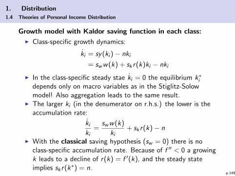
Growth model with Kaldor saving function in each class:
I Class-specific growth dynamics:
ki = sy(ki )− nki
= sww(k) + sk r(k)ki − nki
I In the class-specific steady stae ki = 0 the equilibrium k∗idepends only on macro variables as in the Stiglitz-Solowmodel! Also aggregation leads to the same result.
I The larger ki (in the denumerator on r.h.s.) the lower is theaccumulation rate:
kiki
=sww(k)
ki+ sk r(k)− n
I With the classical saving hypothesis (sw = 0) there is noclass-specific accumulation rate. Because of f ′′ < 0 a growingk leads to a decline of r(k) = f ′(k), and the steady stateimplies sk r(k∗) = n.
p.148
1. Distribution
1.4 Theories of Personal Income Distribution
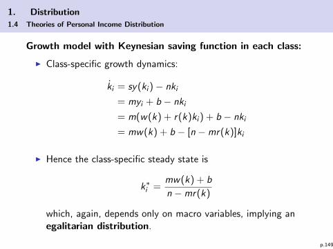
Growth model with Keynesian saving function in each class:
I Class-specific growth dynamics:
ki = sy(ki )− nki
= myi + b − nki
= m(w(k) + r(k)ki ) + b − nki
= mw(k) + b − [n −mr(k)]ki
I Hence the class-specific steady state is
k∗i =mw(k) + b
n −mr(k)
which, again, depends only on macro variables, implying anegalitarian distribution.
p.149
1. Distribution
1.4 Theories of Personal Income Distribution
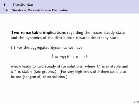
Two remarkable implications regarding the macro steady stateand the dynamics of the distribution towards the steady state:
(i) For the aggregated dynamics we have
k = my(k) + b − nk
which leads to two steady state solutions, where k∗ is unstable andk∗∗ is stable (see graphic)! (For very high levels of b there could also
be one (tangential) or no solution.)
p.150
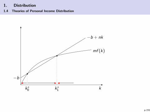
1. Distribution
1.4 Theories of Personal Income Distribution
k
mf (k)
−b
−b + nk
k∗1k∗0
p.151
1. Distribution
1.4 Theories of Personal Income Distribution
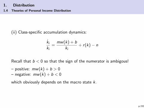
(ii) Class-specific accumulation dynamics:
kiki
=mw(k) + b
ki+ r(k)− n
Recall that b < 0 so that the sign of the numerator is ambigous!
– positive: mw(k) + b > 0– negative: mw(k) + b < 0
which obviously depends on the macro state k.
p.152
1. Distribution
1.4 Theories of Personal Income Distribution
Result:
I If mw(k) + b > 0 then ki/ki increases with decreasing ki =capital stock of less wealthy households grows faster thancapital stock of very wealthy households⇒ convergence of income distribution (inequality ↓).
I If mw(k) + b < 0 then ki/ki decreases with decreasing ki =capital stock of less wealthy households grows slower thancapital stock of very wealthy households⇒ divergence of income distribution (inequality ↑)!
What happens during the accumulation process of k?
p.153
1. Distribution
1.4 Theories of Personal Income Distribution
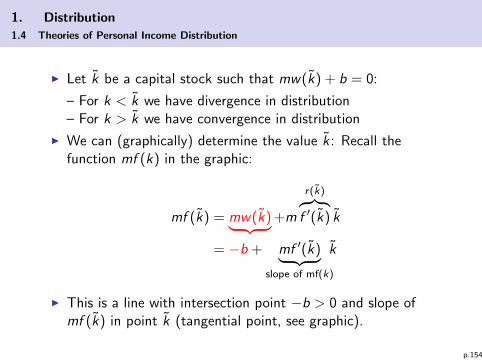
I Let k be a capital stock such that mw(k) + b = 0:
– For k < k we have divergence in distribution– For k > k we have convergence in distribution
I We can (graphically) determine the value k: Recall thefunction mf (k) in the graphic:
mf (k) = mw(k)︸ ︷︷ ︸+m
r(k)︷ ︸︸ ︷f ′(k) k
= −b + mf ′(k)︸ ︷︷ ︸slope of mf(k)
k
I This is a line with intersection point −b > 0 and slope ofmf (k) in point k (tangential point, see graphic).
p.154
1. Distribution
1.4 Theories of Personal Income Distribution
k
mf (k)
−b
−b + nk
k∗1k∗0
−b + sf ′(k)k
k
divergence divergence
of distribution
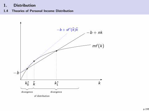
p.155
1. Distribution
1.4 Theories of Personal Income Distribution
I Starting close (right) to unstable steady state k∗0 we have acontinous movement towards the steady state k∗1 but with aninitially increasing inequality (divergence) and then declininginequality (convergence). In k∗1 we end up with an egalitariandistribtion.
I The firstly increasing and then later declining inequality is inline with the Kuznets hypothesis (see previous chapter).
p.156
1. Distribution
1.4 Theories of Personal Income Distribution
General conclusions Stiglitz-Solow type models:
I In Solow, Kaldor, and Keynes variant we have a stableconvergence of aggregated k towards the steady state.
I Only an egalitarian income distribution is consistent with asteady state: k∗i and thus y∗i is identical for all classes.
⇒ counterfactual; convergence to equity of market incomenot in line with empirical picture!
I For the Keynesian variant the inequality of ki (and thus yi )first increases and then declines.
I These results are robust as long as there are savings fromlabor income.
p.157
1. Distribution
1.4 Theories of Personal Income Distribution
Open questions / model variations:
I What happens if we consider class-specific reproduction ratesni? Answer: long-run dynamics leads to asymptotic increaseto population share = 1 for the class with highestreproduction rate.
I Enhancing the model with heterogeneous abilities and HumanCapital (see micro approaches). Answer: ability distributionhas no influence on macro-dynamic; thus the result isdetermined by the initial exogenous ability distribution.
I Implications for functional income distribution (to bediscussed later in a similar framework).
p.158

1. Distribution
1.4 Theories of Personal Income Distribution
Open questions / model variations: (cont.)
I Intertemporal optimization of consumption/saving path (nofixed saving rate). Result: “anything goes”.
I Stochastic influences (e.g. on productivity)
I Imperfect capital markets: agency costs and restriction tolending. Steady-state solutions imply income inequality ;steady-state might be pareto-inefficient (redistribution policydemanded).
(Brief idea: If due to agency problems big firms/investors have
better access to the capital market than small ones, interest rate
might depend on wealth: r = r(ki ) (instead of r(k)). Then the
seady state depends on class-specific variables.)
p.159
1. Distribution
1.4 Theories of Personal Income Distribution
d) Socio-economic arguments
See the slides of the lecture (will not be recapitulated)!
Income inequality among different sociological groups (gender,race, religion, age, family status, ....)
If there is inequality, then:I Either there exist economic reasons which depend on
differences in abilities a, or Human Capital H or financialwealth K ,...
I .. or reasons based on social mechanisms of discrimination(different payments although the (marginal) contibution tothe output is the same),...
I ... or combinations of both, e.g. preventing social groups fromhigher education (investment into H) or from getting jobswhich are matching their abilities a.
p.160
1. Distribution
1.4 Theories of Personal Income Distribution
e) Political Economy of Distribution [to be added]
General idea: Role of the government; incentives of politicians tochange the income distribution.
I Do politicians have an incentive to create inequality in orderto be supported by particular voter groups?
I Which redistributional measures are preferred by the medianvoter (depends on his position in the income distribution)?
⇒ Public Choice approach to income distribution policy.
p.161
1. Distribution
1.4 Theories of Personal Income Distribution
A completely different question comes from (normative) welfaretheory: which redistributional measures a social planner shouldtake?
I This requires a normative theory, e.g. about justice⇒ debatable!
I An easier economic approach: all persons – irrespective oftheir position in the income distribution – might have anincentive to vote for some redistribution as redistributionserves as an insurance against market incomeuncertainty! Uncertainty of effective income is then lowerthan of market income.
I In the latter case there is (to some extent) no trade-offbetween efficiency and redistribution.
p.162
1. Distribution
1.5 Theories of Functional Income Distribution
Functional income distribution: labor share versus capital share
What drives factor prices?
I market structure (e.g. competition, monopolies,...)
I abundancy of the factors (e.g. what happens if capital stockincreases?)
I technical progress (e.g. what happens if technical progressaffects labor productivity?)
I macroeconomic state (e.g. what happens in case of increasingunemployment?)
I policy measures (e.g. what happens in case of minimumwages or monetary expansion?)
p.163
1. Distribution
1.5 Theories of Functional Income Distribution
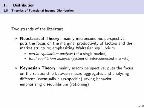
Two strands of the literature:
I Neoclassical Theory: mainly microeconomic perspective;puts the focus on the marginal productivity of factors and themarket structure; emphasizing Walrasian equilibrium
I partial equilibrium analysis (of a single market)I total equilibrium analysis (system of interconnected markets)
I Keynesian Theory: mainly macro perspective; puts the focuson the relationship between macro aggregates and analysingdifferent (eventually class-specific) saving behavior;emphasizing disequilibrium (rationing)
p.164
1. Distribution
1.5 Theories of Functional Income Distribution
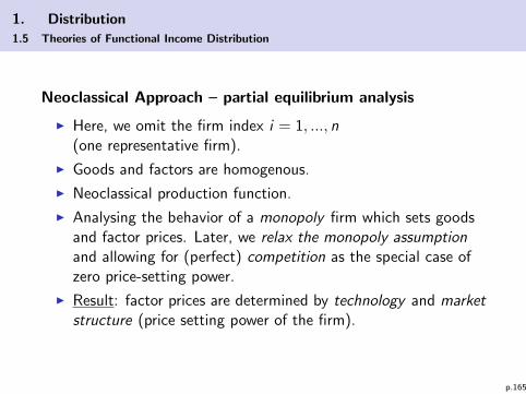
Neoclassical Approach – partial equilibrium analysis
I Here, we omit the firm index i = 1, ..., n(one representative firm).
I Goods and factors are homogenous.
I Neoclassical production function.
I Analysing the behavior of a monopoly firm which sets goodsand factor prices. Later, we relax the monopoly assumptionand allowing for (perfect) competition as the special case ofzero price-setting power.
I Result: factor prices are determined by technology and marketstructure (price setting power of the firm).
p.165
1. Distribution
1.5 Theories of Functional Income Distribution
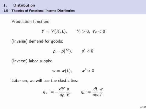
Production function:
Y = Y (K , L), Yi > 0, Yii < 0
(Inverse) demand for goods:
p = p(Y ), p′ < 0
(Inverse) labor supply:
w = w(L), w ′ > 0
Later on, we will use the elasticities:
ηY := −dY
dp
p
Y, ηL :=
dL
dw
w
L
p.166
1. Distribution
1.5 Theories of Functional Income Distribution
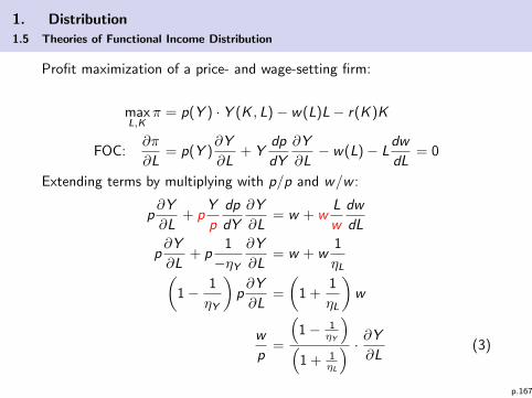
Profit maximization of a price- and wage-setting firm:
maxL,K
π = p(Y ) · Y (K , L)− w(L)L− r(K )K
FOC:∂π
∂L= p(Y )
∂Y
∂L+ Y
dp
dY
∂Y
∂L− w(L)− L
dw
dL= 0
Extending terms by multiplying with p/p and w/w :
p∂Y
∂L+ p
Y
p
dp
dY
∂Y
∂L= w + w
L
w
dw
dL
p∂Y
∂L+ p
1
−ηY∂Y
∂L= w + w
1
ηL(1− 1
ηY
)p∂Y
∂L=
(1 +
1
ηL
)w
w
p=
(1− 1
ηY
)(
1 + 1ηL
) · ∂Y
∂L(3)
p.167
1. Distribution
1.5 Theories of Functional Income Distribution
w
p=
(1− 1
ηY
)(
1 + 1ηL
) · ∂Y
∂L
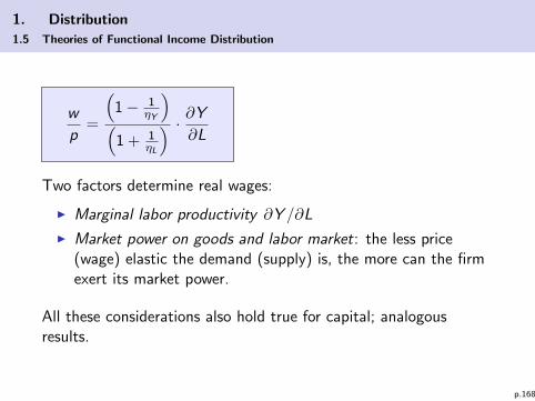
Two factors determine real wages:
I Marginal labor productivity ∂Y /∂L
I Market power on goods and labor market: the less price(wage) elastic the demand (supply) is, the more can the firmexert its market power.
All these considerations also hold true for capital; analogousresults.
p.168
1. Distribution
1.5 Theories of Functional Income Distribution
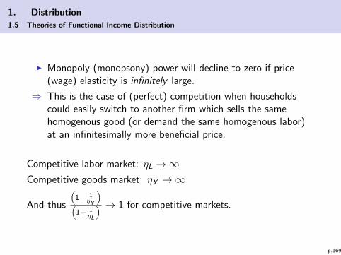
I Monopoly (monopsony) power will decline to zero if price(wage) elasticity is infinitely large.
⇒ This is the case of (perfect) competition when householdscould easily switch to another firm which sells the samehomogenous good (or demand the same homogenous labor)at an infinitesimally more beneficial price.
Competitive labor market: ηL →∞Competitive goods market: ηY →∞
And thus
(1− 1
ηY
)(
1+ 1ηL
) → 1 for competitive markets.
p.169
1. Distribution
1.5 Theories of Functional Income Distribution
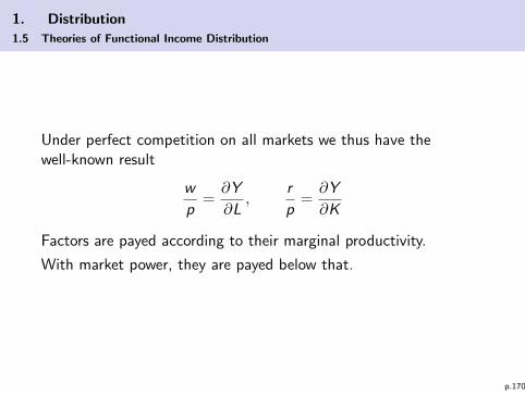
Under perfect competition on all markets we thus have thewell-known result
w
p=∂Y
∂L,
r
p=∂Y
∂K
Factors are payed according to their marginal productivity.
With market power, they are payed below that.
p.170
1. Distribution
1.5 Theories of Functional Income Distribution
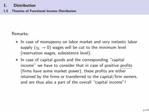
Remarks:
I In case of monopsony on labor market and very inelastic laborsupply (ηL → 0) wages will be cut to the minimum level(reservation wages, subsistence level).
I In case of capital goods and the corresponding “capitalincome” we have to consider that in case of positive profits(firms have some market power), these profits are eitherretained by the firms or transferred to the capital/firm owners,and are thus also a part of the overall “capital income”!
p.171
1. Distribution
1.5 Theories of Functional Income Distribution
In case of capital the formalism is basically the same. However, theinterpretation is slightly different:
I Firms do not “hire” capital but buy capital goods. They haveto finance these costs.
I They can either use own savings (internal financing) orfinancing these costs externally by issuing bonds or equitycapital or they demand loans. In all these cases the owners ofthe firm or the creditors have claims such like interest rate ordividend payments.
I We assume perfect capital markets (no transaction costs, noagency problems, complete future markets). Thus we have auniform capital cost r per unit of capital.
p.172
1. Distribution
1.5 Theories of Functional Income Distribution
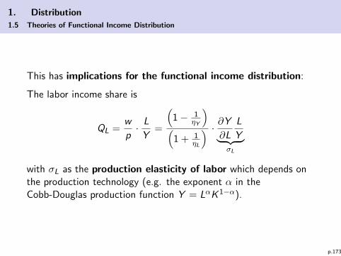
This has implications for the functional income distribution:
The labor income share is
QL =w
p· L
Y=
(1− 1
ηY
)(
1 + 1ηL
) · ∂Y
∂L
L
Y︸ ︷︷ ︸σL
with σL as the production elasticity of labor which depends onthe production technology (e.g. the exponent α in theCobb-Douglas production function Y = LαK 1−α).
p.173
1. Distribution
1.5 Theories of Functional Income Distribution
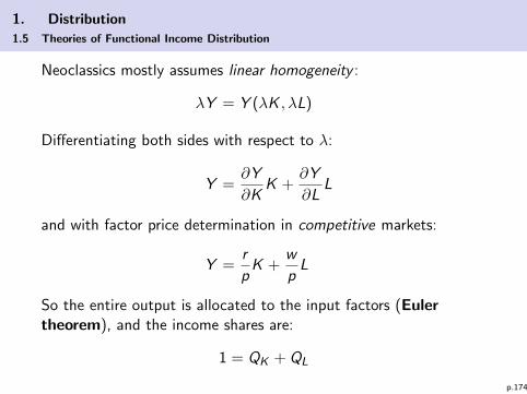
Neoclassics mostly assumes linear homogeneity :
λY = Y (λK , λL)
Differentiating both sides with respect to λ:
Y =∂Y
∂KK +
∂Y
∂LL
and with factor price determination in competitive markets:
Y =r
pK +
w
pL
So the entire output is allocated to the input factors (Eulertheorem), and the income shares are:
1 = QK + QL
p.174
1. Distribution
1.5 Theories of Functional Income Distribution
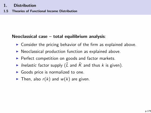
Neoclassical case – total equilibrium analysis:
I Consider the pricing behavior of the firm as explained above.
I Neoclassical production function as explained above.
I Perfect competition on goods and factor markets.
I Inelastic factor supply (L and K and thus k is given).
I Goods price is normalized to one.
I Then, also r(k) and w(k) are given.
p.175
1. Distribution
1.5 Theories of Functional Income Distribution
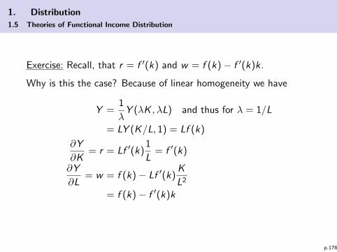
Exercise: Recall, that r = f ′(k) and w = f (k)− f ′(k)k .
Why is this the case? Because of linear homogeneity we have
Y =1
λY (λK , λL) and thus for λ = 1/L
= LY (K/L, 1) = Lf (k)
∂Y
∂K= r = Lf ′(k)
1
L= f ′(k)
∂Y
∂L= w = f (k)− Lf ′(k)
K
L2
= f (k)− f ′(k)k
p.176
1. Distribution
1.5 Theories of Functional Income Distribution
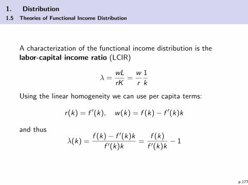
A characterization of the functional income distribution is thelabor-capital income ratio (LCIR)
λ =wL
rK=
w
r
1
k
Using the linear homogeneity we can use per capita terms:
r(k) = f ′(k), w(k) = f (k)− f ′(k)k
and thus
λ(k) =f (k)− f ′(k)k
f ′(k)k=
f (k)
f ′(k)k− 1
p.177
1. Distribution
1.5 Theories of Functional Income Distribution
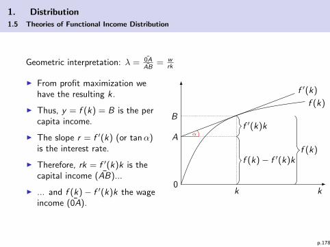
Geometric interpretation: λ = 0AAB
= wrk
I From profit maximization wehave the resulting k .
I Thus, y = f (k) = B is the percapita income.
I The slope r = f ′(k) (or tanα)is the interest rate.
I Therefore, rk = f ′(k)k is thecapital income (AB)...
I ... and f (k)− f ′(k)k the wageincome (0A).
k0
f (k)
k
B
f ′(k)
A αf ′(k)k
f (k)− f ′(k)kf (k)
p.178
1. Distribution
1.5 Theories of Functional Income Distribution
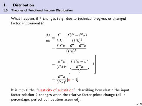
What happens if k changes (e.g. due to technical progress or changedfactor endowment)?
dλ
dk=
f ′
f ′k− f (f ′ − f ′′k)
(f ′k)2
=f ′f ′k − ff ′ − ff ′′k
(f ′k)2
=ff ′′k
(f ′k)2
f ′f ′k − ff ′
ff ′′k︸ ︷︷ ︸σ
−1
=
ff ′′k
(f ′k)2[σ − 1]
It is σ > 0 the “elasticity of substition”, describing how elastic the inputfactor relation k changes when the relative factor prices change (all inpercentage, perfect competition assumed).
p.179
1. Distribution
1.5 Theories of Functional Income Distribution
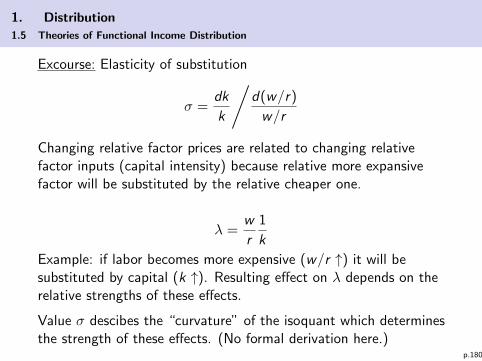
Excourse: Elasticity of substitution
σ =dk
k
/d(w/r)
w/r
Changing relative factor prices are related to changing relativefactor inputs (capital intensity) because relative more expansivefactor will be substituted by the relative cheaper one.
λ =w
r
1
k
Example: if labor becomes more expensive (w/r ↑) it will besubstituted by capital (k ↑). Resulting effect on λ depends on therelative strengths of these effects.
Value σ descibes the “curvature” of the isoquant which determinesthe strength of these effects. (No formal derivation here.)
p.180

1. Distribution
1.5 Theories of Functional Income Distribution
Recall that f ′′ < 0. Hence we have
dλ/dk > 0 ⇐⇒ σ < 1
dλ/dk = 0 ⇐⇒ σ = 1
dλ/dk < 0 ⇐⇒ σ > 1
The effect of a changing k on the functional income distributiondepends on the properties of the production technology !
Linear-homogenous Cobb-Douglas function has σ = 1 and thus wehave no effect on income distribution.
p.181
1. Distribution
1.5 Theories of Functional Income Distribution
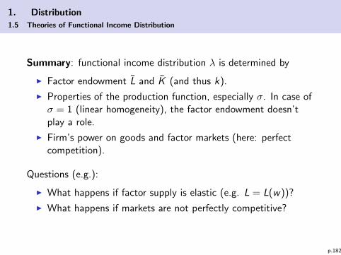
Summary: functional income distribution λ is determined by
I Factor endowment L and K (and thus k).
I Properties of the production function, especially σ. In case ofσ = 1 (linear homogeneity), the factor endowment doesn’tplay a role.
I Firm’s power on goods and factor markets (here: perfectcompetition).
Questions (e.g.):
I What happens if factor supply is elastic (e.g. L = L(w))?
I What happens if markets are not perfectly competitive?
p.182
1. Distribution
1.5 Theories of Functional Income Distribution
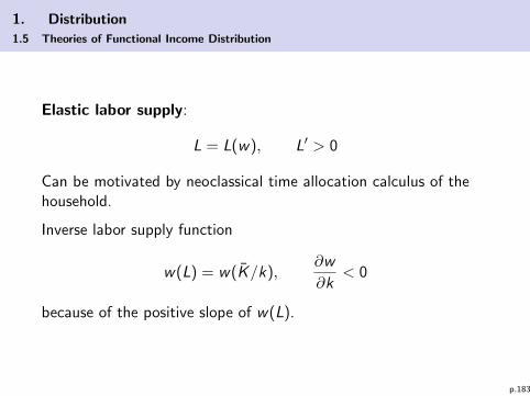
Elastic labor supply:
L = L(w), L′ > 0
Can be motivated by neoclassical time allocation calculus of thehousehold.
Inverse labor supply function
w(L) = w(K/k),∂w
∂k< 0
because of the positive slope of w(L).
p.183
1. Distribution
1.5 Theories of Functional Income Distribution
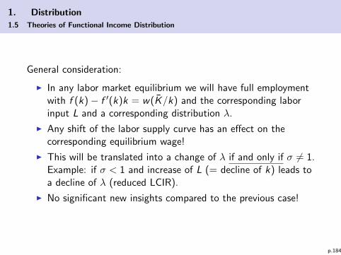
General consideration:
I In any labor market equilibrium we will have full employmentwith f (k)− f ′(k)k = w(K/k) and the corresponding laborinput L and a corresponding distribution λ.
I Any shift of the labor supply curve has an effect on thecorresponding equilibrium wage!
I This will be translated into a change of λ if and only if σ 6= 1.Example: if σ < 1 and increase of L (= decline of k) leads toa decline of λ (reduced LCIR).
I No significant new insights compared to the previous case!
p.184
1. Distribution
1.5 Theories of Functional Income Distribution
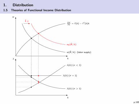
w
kλ
k
∂Y∂L
= f (k)− f ′(k)k
w(K/k) (labor supply)
w1(K/k)
L ↓
λ(k) (σ < 1)
λ(k) (σ = 1)
λ(k) (σ > 1)
p.185
1. Distribution
1.5 Theories of Functional Income Distribution
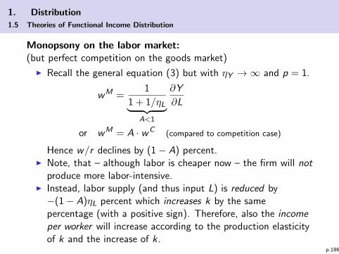
Monopsony on the labor market:(but perfect competition on the goods market)
I Recall the general equation (3) but with ηY →∞ and p = 1.
wM =1
1 + 1/ηL︸ ︷︷ ︸A<1
∂Y
∂L
or wM = A · wC (compared to competition case)
Hence w/r declines by (1− A) percent.I Note, that – although labor is cheaper now – the firm will not
produce more labor-intensive.I Instead, labor supply (and thus input L) is reduced by−(1− A)ηL percent which increases k by the samepercentage (with a positive sign). Therefore, also the incomeper worker will increase according to the production elasticityof k and the increase of k .
p.186
1. Distribution
1.5 Theories of Functional Income Distribution
I But this implies for the LCIR:
λM(kM) =wM
f (kM)− wM=
AwC
f (kM)− AwC<
wC
f (kC )− wC= λC (kC )
Note that these two λ-values are not for the same k .Result: With monopsony power income distribution changesin favor of the capital share.
I For any given value of k the numerator of λM is smaller andthe denumerator larger than in case of λC , thus theλ(k)-function is flatter in the monopsony case.
I However, the dependency ∂λ/∂k R 0 again depends on theelasticity of substitution.
p.187
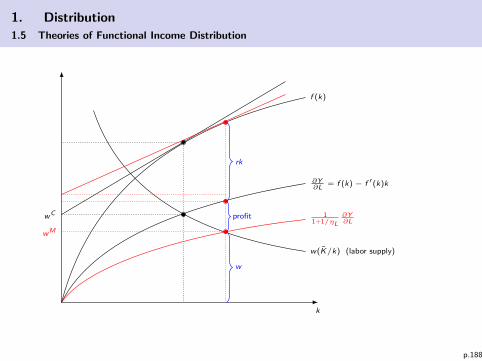
1. Distribution
1.5 Theories of Functional Income Distribution
k
∂Y∂L
= f (k)− f ′(k)k
w(K/k) (labor supply)
f (k)
wC 11+1/ηL
∂Y∂L
wM
rk
w
profit
p.188
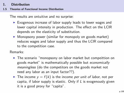
1. Distribution
1.5 Theories of Functional Income Distribution
The results are ontuitive and no surprise:
I Exogenous increase of labor supply leads to lower wages andlower capital intensity in production. The effect on the LCIRdepends on the elasticity of substitution.
I Monopsony power (similar for monopoly on goods market)reduces wages and labor supply and thus the LCIR comparedto the competition case.
Remarks:
I The scenario “monopsony on labor market but compeittion ongoods market” is mathematically possible but economicallymeaningless (do the competitors on the goods market notneed any labor as an input factor??).
I The income y = f (k) is the income per unit of labor, not percapita, if labor supply is elastic. Only if L is exogenously givenit is a good proxy for “capita”.
p.189
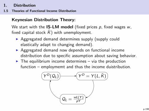
1. Distribution
1.5 Theories of Functional Income Distribution
Keynesian Distribution Theory:
We start with the IS-LM model (fixed prices p, fixed wages w ,fixed capital stock K ) with unemployment.
I Aggregated demand determines supply (supply couldelastically adapt to changing demand).
I Aggregated demand now depends on functional incomedistribution due to specific assumption about saving behavior.
I The equilibrium income determines – via the productionfunction – employmemt and thus the income duistribution.
Y D(QL) Y D = Y (L, K )
QL = wL(Y )pY
p.190
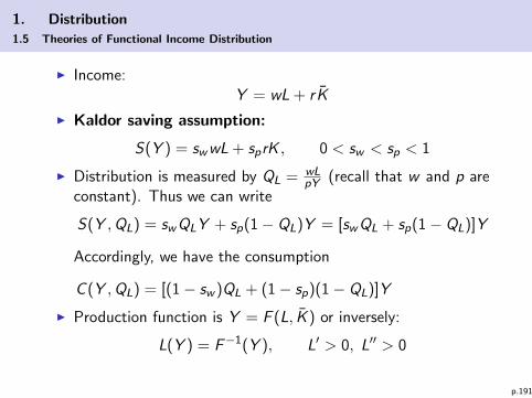
1. Distribution
1.5 Theories of Functional Income Distribution
I Income:Y = wL + r K
I Kaldor saving assumption:
S(Y ) = swwL + sprK , 0 < sw < sp < 1
I Distribution is measured by QL = wLpY (recall that w and p are
constant). Thus we can write
S(Y ,QL) = swQLY + sp(1− QL)Y = [swQL + sp(1− QL)]Y
Accordingly, we have the consumption
C (Y ,QL) = [(1− sw )QL + (1− sp)(1− QL)]Y
I Production function is Y = F (L, K ) or inversely:
L(Y ) = F−1(Y ), L′ > 0, L′′ > 0
p.191
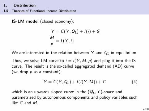
1. Distribution
1.5 Theories of Functional Income Distribution
IS-LM model (closed economy):
Y = C (Y ,QL) + I (i) + G
M
p= L(Y , i)
We are interested in the relation between Y and QL in equilibrium.
Thus, we solve LM curve to i = i(Y ,M, p) and plug it into the IScurve. The result is the so-called aggregated demand (AD) curve(we drop p as a constant):
Y = C (Y ,QL) + I (i(Y ,M)) + G (4)
which is an upwards sloped curve in the (QL,Y )-space andparametrized by autonomous components and policy variables suchlike G and M.
p.192
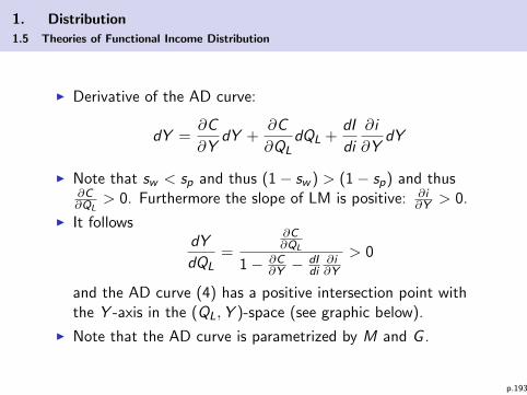
1. Distribution
1.5 Theories of Functional Income Distribution
I Derivative of the AD curve:
dY =∂C
∂YdY +
∂C
∂QLdQL +
dI
di
∂i
∂YdY
I Note that sw < sp and thus (1− sw ) > (1− sp) and thus∂C∂QL
> 0. Furthermore the slope of LM is positive: ∂i∂Y > 0.
I It followsdY
dQL=
∂C∂QL
1− ∂C∂Y −
dIdi
∂i∂Y
> 0
and the AD curve (4) has a positive intersection point withthe Y -axis in the (QL,Y )-space (see graphic below).
I Note that the AD curve is parametrized by M and G .
p.193
1. Distribution
1.5 Theories of Functional Income Distribution
I Note that the AD curve depicts the equilibrium income Y fora given QL. However, there cannot be an arbitrary relationbetween Y and QL because of the technological relationbetween labor and output:
QL(Y ) =wL(Y )
pY(5)
I Without loss of generality let us assume w = p = 1.
p.194
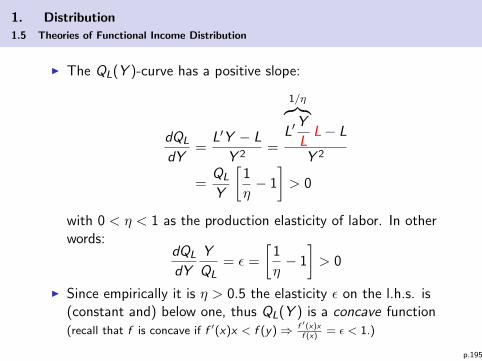
1. Distribution
1.5 Theories of Functional Income Distribution
I The QL(Y )-curve has a positive slope:
dQL
dY=
L′Y − L
Y 2=
1/η︷︸︸︷L′
Y
LL− L
Y 2
=QL
Y
[1
η− 1
]> 0
with 0 < η < 1 as the production elasticity of labor. In otherwords:
dQL
dY
Y
QL= ε =
[1
η− 1
]> 0
I Since empirically it is η > 0.5 the elasticity ε on the l.h.s. is(constant and) below one, thus QL(Y ) is a concave function(recall that f is concave if f ′(x)x < f (y)⇒ f ′(x)x
f (x)= ε < 1.)
p.195
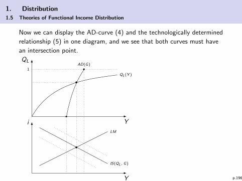
1. Distribution
1.5 Theories of Functional Income Distribution
Now we can display the AD-curve (4) and the technologically determined
relationship (5) in one diagram, and we see that both curves must have
an intersection point.
QL
Y
1
i
Y
LM
IS(QL, G)
AD(G)
QL(Y )
p.196
1. Distribution
1.5 Theories of Functional Income Distribution
Policy variation:
I The AD curve can be shifted by monetary or fiscal policy (Mor G ) (right-shift of either LM or IS curve in theIS-LM-scheme ⇒ right-shift AD).
I Thus increased aggregated demand induces higher outputwhich induces higher employment which then leads to achange in the functional income distribution (increase of QL)!
p.197
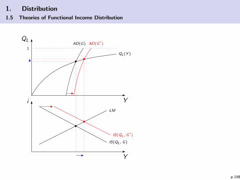
1. Distribution
1.5 Theories of Functional Income Distribution
QL
Y
1
i
Y
LM
IS(QL, G)
AD(G)
QL(Y )
IS(QL, G′)
AD(G ′)
p.198
1. Distribution
1.5 Theories of Functional Income Distribution
I Functional income distribution is determined by unemploymentand is thus affected by aggregated demand management.
I Note, that this result does not critically rely on the Kaldorsaving hypothesis. Also with a uniform saving rate(sw = sp = s) the AD curve would not depend on QL (verticalline in graphic) but could be shifted by aggregated demandmanagement.
I Things become more complicated in a flex-price model: Thesupply Y will increase only because the increased demandinduces a rise of the price level p and thus a decline of realwages w/p (which have been assumed to be fixed in theprevious model).
p.199
1. Distribution
1.5 Theories of Functional Income Distribution
Further aspects of functional income distribution:
A) Technological progress (TP)(more about that in module MW21.4)
I TP has an impact on labor and/or capital productivity;“factor augmenting” effect.
I TP is called neutral if it does not have an effect on theincome distribution λ.
I Various forms of TP, not all of them are consistent with asteady-state solution in the Solow growth model.
p.200
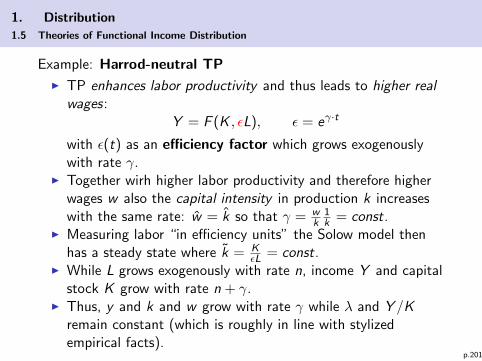
1. Distribution
1.5 Theories of Functional Income Distribution
Example: Harrod-neutral TP
I TP enhances labor productivity and thus leads to higher realwages:
Y = F (K , εL), ε = eγ·t
with ε(t) as an efficiency factor which grows exogenouslywith rate γ.
I Together wirh higher labor productivity and therefore higherwages w also the capital intensity in production k increaseswith the same rate: w = k so that γ = w
k1k = const.
I Measuring labor “in efficiency units” the Solow model thenhas a steady state where k = K
εL = const.I While L grows exogenously with rate n, income Y and capital
stock K grow with rate n + γ.I Thus, y and k and w grow with rate γ while λ and Y /K
remain constant (which is roughly in line with stylizedempirical facts).
p.201
1. Distribution
1.5 Theories of Functional Income Distribution
B) International trade aspects(more about that in module MW21.5)
B.1) Classical trade theory (Ricardo)
I Comparative advantages because of different technologies =different relative labor productivities in the sectors ⇒ everycountry specializes on the good and exports it where it has acomparative advantage.
I Participation in specialization and trade is possible even if theoverall labor productivity in country A is lower than incounrtry B (as long as there are comparative advantages).
I As a result, international differences in factor prices (here:wages) reflect the differences in the labor productivity!
I There is no equalization of factor prices as long as thetechnologies are different.
p.202
1. Distribution
1.5 Theories of Functional Income Distribution
B.2) Neoclassical theory (Heckscher/Ohlin)
I Technologies and thus productivitis are the same across thecountries. Comparative advantages come from different factorendowments (different relative scarcities and thus prices offactors).
I Capital (labor) abundant countries will specialize on thecapital (labor) intensive goods and export them.
I Technologically, there is an unambigous relationshipbetween goods prices and factor prices (coming fromminimal cost production and assumption of perfectcompetition):
pi = ci (w , r), i = 1, 2
I This system of equation has one solution. Since bothcountries use the same technology, and since internationaltrade equalizes the prices p1, p2, as a consequence, the factorprices are equalized as well! p.203
1. Distribution
1.6 Diastribution Policy
Some implications for wage bargaining
1) Distribution-neutral wage-setting
I Let v = Y /L denote the labor productivity. Then:
QL =w
p
L
Y=
w
p
1
v
⇒ QL = w − p − v!
= 0
⇒ w = p + v
⇒ Wages should increase according to inflation rate and theincrease of labor productivity in order to ensure a constantfunctional income distribution.
I Increase of labor productivity due to technical progress.
p.204
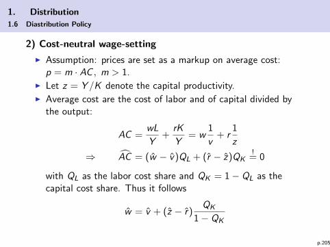
1. Distribution
1.6 Diastribution Policy
2) Cost-neutral wage-setting
I Assumption: prices are set as a markup on average cost:p = m · AC , m > 1.
I Let z = Y /K denote the capital productivity.I Average cost are the cost of labor and of capital divided by
the output:
AC =wL
Y+
rK
Y= w
1
v+ r
1
z
⇒ AC = (w − v)QL + (r − z)QK!
= 0
with QL as the labor cost share and QK = 1− QL as thecapital cost share. Thus it follows
w = v + (z − r)QK
1− QK
p.205
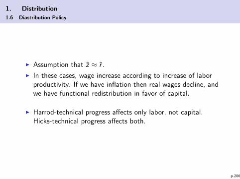
1. Distribution
1.6 Diastribution Policy
I Assumption that z ≈ r .
I In these cases, wage increase according to increase of laborproductivity. If we have inflation then real wages decline, andwe have functional redistribution in favor of capital.
I Harrod-technical progress affects only labor, not capital.Hicks-technical progress affects both.
p.206
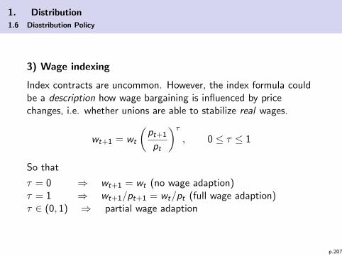
1. Distribution
1.6 Diastribution Policy
3) Wage indexing
Index contracts are uncommon. However, the index formula couldbe a description how wage bargaining is influenced by pricechanges, i.e. whether unions are able to stabilize real wages.
wt+1 = wt
(pt+1
pt
)τ, 0 ≤ τ ≤ 1
So that
τ = 0 ⇒ wt+1 = wt (no wage adaption)τ = 1 ⇒ wt+1/pt+1 = wt/pt (full wage adaption)τ ∈ (0, 1) ⇒ partial wage adaption
p.207
2. Poverty
2.1 Basic ideas and definitions
What does “poor” and “poverty” mean?
Insufficient supply of basic needs:nutrition, health, clothes, dwelling,...
I What is “basic”?
I What is “insufficient”?
I Poverty as the inability or deprivation of a person to supplyhis/her basic needs ⇒ dependency on the help of others inorder to supply the basic wants? (“Capability approach” to bediscussed later)
I What about “voluntary poverty” (e.g. for religious reasons)?If a person would be able to supply the basic needs butchooses not to do so, should it considered as poor?
p.208
2. Poverty
2.1 Basic ideas and definitions
I Meaning of poverty depends on subjective and culturalevaluations.
I Comparable with the subjective well-being as a basis for“wealth” (opposed to “poverty”).
⇒ any measurement concept requires a sound normative basis!
⇒ One of the most fundamental problems: subjective well-being(and thus also poverty) in terms of utility is incommensurable.No objective measure exists which could be comparedbetween individuals and which could be aggregated.
p.209
2. Poverty
2.1 Basic ideas and definitions
I Different indicators for poverty / poverty dimensions:
I Hunger; no access to food (too less calories per day)I Bad health state, insufficient medical supplyI Low life expectancyI Insufficient access to education; illiteracy
I Many basic needs could (and would) be supplied if there is asufficient income.
I Thus, the income might be a – though highly debatable –proxy for poverty. Necessary to define an income threshold :with an income below this threhold it is not possible to supplythe basic needs.
p.210
2. Poverty
2.1 Basic ideas and definitions
I Alternatively, one could construct an index, based on a list ofcriteria (see below).
I Any attempt to aggregate multiple dimensions of subjectivewell-being (or poverty) and adding it up to an aggregatedmeasure is somehow “ad hoc”.
I Moreover, aggregation of different criteria implicitly assumesthat different dimensions of poverty could be weighted againstothers, e.g. less calories per day but higher literacy = samepoverty level?
p.211
2. Poverty
2.2 Poverty measurement
Agenda:
A) Income-based indices:
A.1) Absolute povertyA.2) Relative poverty
B) Normative basis: Sen’s Capability Approach
C) Index constructions based on multidimensional criteria
p.212
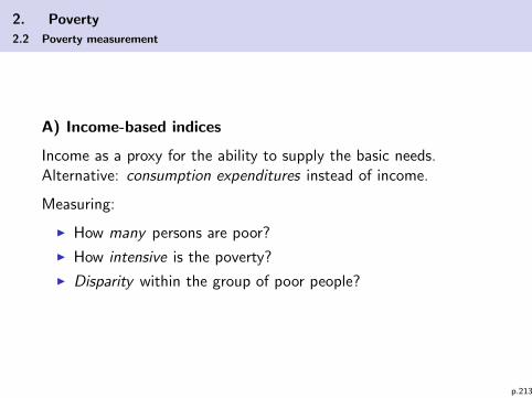
2. Poverty
2.2 Poverty measurement
A) Income-based indices
Income as a proxy for the ability to supply the basic needs.Alternative: consumption expenditures instead of income.
Measuring:
I How many persons are poor?
I How intensive is the poverty?
I Disparity within the group of poor people?
p.213
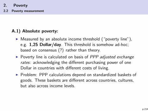
2. Poverty
2.2 Poverty measurement
A.1) Absolute poverty:
I Measured by an absolute income threshold (“poverty line”),e.g. 1,25 Dollar/day. This threshold is somehow ad-hoc;based on consensus (?) rather than theory.
I Poverty line is calculated on basis of PPP adjusted exchangerates: acknowledging the different purchasing power of oneDollar in countries with different costs of living.
I Problem: PPP calculations depend on standardized baskets ofgoods. These baskets are different across countries, cultures,but also across income levels.
p.214
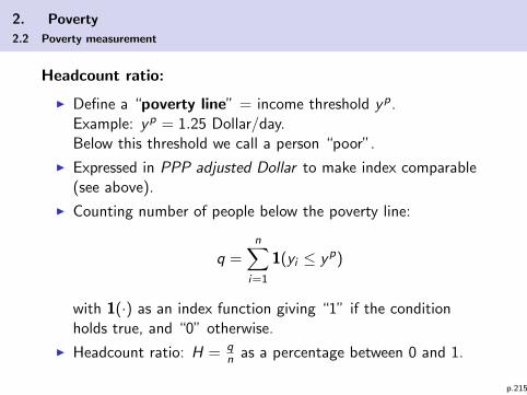
2. Poverty
2.2 Poverty measurement
Headcount ratio:
I Define a “poverty line” = income threshold yp.Example: yp = 1.25 Dollar/day.Below this threshold we call a person “poor”.
I Expressed in PPP adjusted Dollar to make index comparable(see above).
I Counting number of people below the poverty line:
q =n∑
i=1
1(yi ≤ yp)
with 1(·) as an index function giving “1” if the conditionholds true, and “0” otherwise.
I Headcount ratio: H = qn as a percentage between 0 and 1.
p.215
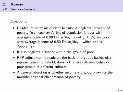
2. Poverty
2.2 Poverty measurement
Objections:
I Headcount index insufficient because it neglects intensity ofpoverty (e.g. country A: 6% of population is poor withaverage income of 0.99 Dollar/day; country B: 3% are poorwith average income of 0,50 Dollar/day – which one is“poorer”?)
I It also neglects disparity within the group of poor.
I PPP adjustment is made on the basis of a goods basket of arepresentative household; does not reflect diffreent behavior ofpoor people in different cultures.
I A general objection is whether income is a good proxy for themultidimensional phenomenon of poverty.
p.216
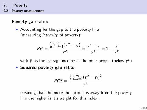
2. Poverty
2.2 Poverty measurement
Poverty gap ratio:
I Accounting for the gap to the poverty line(measuring intensity of poverty):
PG =
1q
∑qi=1(yp − yi )
yp=
yp − y
yp= 1− y
yp
with y as the average income of the poor people (below yp).
I Squared poverty gap ratio:
PGS =
1q
∑qi=1(yp − yi )
2
yp
meaning that the more the income is away from the povertyline the higher is it’s weight for this index.
p.217
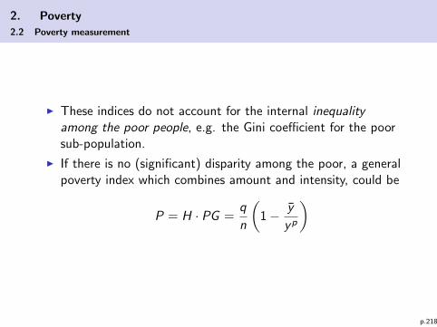
2. Poverty
2.2 Poverty measurement
I These indices do not account for the internal inequalityamong the poor people, e.g. the Gini coefficient for the poorsub-population.
I If there is no (significant) disparity among the poor, a generalpoverty index which combines amount and intensity, could be
P = H · PG =q
n
(1− y
yp
)
p.218
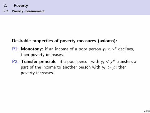
2. Poverty
2.2 Poverty measurement
Desirable properties of poverty measures (axioms):
P1: Monotony: if an income of a poor person yi < yp declines,then poverty increases.
P2: Transfer principle: if a poor person with yi < yp transfers apart of the income to another person with yk > yi , thenpoverty increases.
p.219
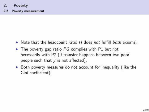
2. Poverty
2.2 Poverty measurement
I Note that the headcount ratio H does not fulfill both axioms!
I The poverty gap ratio PG complies with P1 but notnecessarily with P2 (if transfer happens between two poorpeople such that y is not affected).
I Both poverty measures do not account for inequality (like theGini coefficient).
p.220
2. Poverty
2.2 Poverty measurement
I Headcount ratio also responds if the number of rich peopleincreases while the life situation of all poor people remains thesame (division of q by a larger n).
I Obviously, H and PG do not respond to changes of theincome of “rich” persons (yj > yp), or in other words: to thedisparity between rich and poor – since it meassures absolutepoverty.
I What happens if yp increases (re-alignment of the povertyline)? Obviously H must increase as well! Because y mighteventually increase more than the number of poor people, theeffect on PG is not clear.
p.221
2. Poverty
2.2 Poverty measurement
Some critical remarks:
I Even with income below the poverty line it might be possibleto have enough calories (e.g. self-provided agriculturalproducts).
I Even above the poverty line it might be not possible to servefor the basic needs.
I The income measure assumes that income is completely usedfor serving for the basic needs:
Empirically, this is questionable: very poor people often spendmoney for alcohol, cigarettes, electronics, or they save moneyin order to spent it for very expensive marriage ceremonies orfunerals etc.
A poverty measure should respect different preferencesregarding the “poor life”.
p.222
2. Poverty
2.2 Poverty measurement
A.2) Relative poverty
I Which needs are “basic”? Could depend on cultural andsocial environment.
I Example: participation in social life; integration in socialcommunity rather than marginalization.
I Marginalization and social exclusion might depend on theincome gap between the poor person and the peer group
⇒ a person is “poor” relative to others.
p.223
2. Poverty
2.2 Poverty measurement
(Bad) Example:
I The first 5%-quantile of the income distribution could becalled “poor”.
I This doesn’t say anything about the entire distribution. Arethese 5% still poor if the Gini is close to zero?
I This measurement is uninformative because per definition 5%of the population are always and necessarily poor, irrespectiveof any poverty reduction policies.
⇒ Not reasonable!
p.224
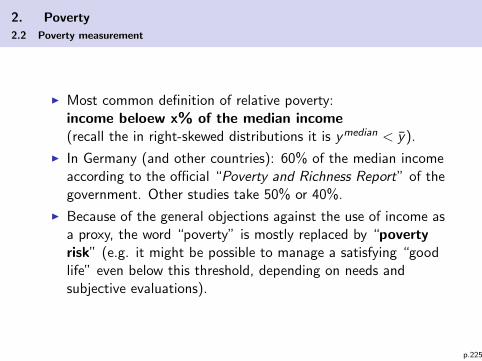
2. Poverty
2.2 Poverty measurement
I Most common definition of relative poverty:income beloew x% of the median income(recall the in right-skewed distributions it is ymedian < y).
I In Germany (and other countries): 60% of the median incomeaccording to the official “Poverty and Richness Report” of thegovernment. Other studies take 50% or 40%.
I Because of the general objections against the use of income asa proxy, the word “poverty” is mostly replaced by “povertyrisk” (e.g. it might be possible to manage a satisfying “goodlife” even below this threshold, depending on needs andsubjective evaluations).
p.225
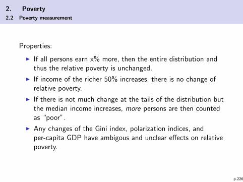
2. Poverty
2.2 Poverty measurement
Properties:
I If all persons earn x% more, then the entire distribution andthus the relative poverty is unchanged.
I If income of the richer 50% increases, there is no change ofrelative poverty.
I If there is not much change at the tails of the distribution butthe median income increases, more persons are then countedas “poor”.
I Any changes of the Gini index, polarization indices, andper-capita GDP have ambigous and unclear effects on relativepoverty.
p.226
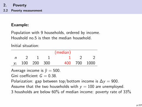
2. Poverty
2.2 Poverty measurement
Example:
Population with 9 households, ordered by income.Houshold no.5 is then the median household.
Initial situation:
(median)n 2 1 1 1 2 2yi 100 200 300 400 700 1000
Average income is y = 500.Gini coefficient G = 0.38.Polarization: gap between top/bottom income is ∆y = 900.Assume that the two households with y = 100 are unemployed.3 housholds are below 60% of median income: poverty rate of 33%
p.227
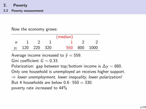
2. Poverty
2.2 Poverty measurement
Now the economy grows:
(median)n 1 2 1 1 2 2yi 120 220 320 550 800 1000
Average income increased to y = 559.Gini coefficient G = 0.33.Polarization: gap between top/bottom income is ∆y = 880.Only one household is unemployed an receives higher support.⇒ lower unemployment, lower inequality, lower polarization!But 4 households are below 0.6 · 550 = 330:poverty rate increased to 44%
p.228
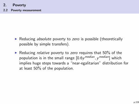
2. Poverty
2.2 Poverty measurement
I Reducing absolute poverty to zero is possible (theoreticallypossible by simple transfers).
I Reducing relative poverty to zero requires that 50% of thepopulation is in the small range [0.6ymedian, ymedian] whichimplies huge steps towards a “near-egalitarian” distribution forat least 50% of the population.
p.229
2. Poverty
2.2 Poverty measurement
Relative poverty in a rich economy like Germany:
I Social security system should guarantee an income which issufficient for the “subsistence level” (basic needs for food, clothes,accomodation etc. but also – to a small extent – participation atsocial life and culture). In Germany: SGB II (so-called “Hartz IV ”).
I However, the legally defined minimum or subsistence level might bebelow the poverty threshold of 60% of the median income (de facto:ca. 45%).
I Germany 2014: median income is always calculated as netequivalence household income (see chapter 1). “Poor” is a singleperson household with 917 Euro, and a household with 2 parentsand two children with 1926 Euro. Poverty rate was round about15%.
p.230
2. Poverty
2.2 Poverty measurement
Reasons:
I (Long-term) unemployment⇒ income declines to subsistence support (SGB II).
I “Non-standard work contracts”: part-time jobs, temporaryemployment, labor lessing⇒ insufficient income, “working poor”
I Due to demographic change: cuts (or freezed) retirementpayments where older people do not have a chance to increaseit by part-time jobs.
More about global economic conditions and consequences ofpoverty will be discussed later on.
p.231
2. Poverty
2.2 Poverty measurement
B) Sen’s Capability Approach:
I We return to the fundamental aspect of poverty as “inabilityto supply the basic needs”.
I Sen’s approach comes from social philosophy, reflecting thenormative grounds on assessing a situation as “poverty”.
I It is based on the idea of freedom: a situation should beevaluated according to the extent of freedom people have toachieve functionings they value.
I Since freedom is understood as metrial, effective freedom, andjustice is related to the opportunities to manage one’s ownlife, poverty is also linked to the Theory of Justice.
p.232

2. Poverty
2.2 Poverty measurement
I Functionings: things people value to do or to be (thingswhich supply their needs). Different functionings constitute afunctioning vector or bundle.
I Capability: set of functioning bundles which a person couldeffectively achieve.
I Freedom means that people can choose functionings fromthis set according to their personal needs or personal ideasabout a “good life”.
⇒ Hence, capability includes both, achievable functionings andthe freedom to choose them.
I Functionings require resources. Some resources are related tothe individual person (e.g. health, skills), some others aredetermined by social and economic conditions.
p.233
2. Poverty
2.2 Poverty measurement
Examples:Resource: Food Political institutions Healthcare systemCapability: Ability to be nourished Political participation Access to HCSFunctioning: Being nourished Voting power Health
I The functionings are chosen according to the valuation of theperson ⇒ intrinsic utility.
I However, intrinsic utility is neither measurable norinterpresonally comparable.
I Functionings, in contrast, allow for a much bettermeasurement and comparability.
p.234
2. Poverty
2.2 Poverty measurement
Important implications:
I Freedom as the real opportunity to accomplish what we value,not only an abtrsact right to do something. Effective freedomrequires capabilities.
I It is the individual and her ideas about a “good life” whichleads her to a choice of functionings – not primarly the ideasof the rich about what poor people are lacking.
I Freedom to choose your own life as a person within acommunity.
I Thus, poverty reduction does not mean that we supply poorpeople with goods or functionings but enlarge their capability.
p.235

2. Poverty
2.2 Poverty measurement
Two aspects of freedom:
I The capabilities reflect the opportunity aspect of freedom (ifcapabilities are zero then there is nothing to choose).
I The agency aspect reflects the ability to act, to changethings according to own objectives and values: “what aperson is free to do and achieve in pursuit of whatever goalsor values he or she regards as important.” (A. Sen)
p.236

2. Poverty
2.2 Poverty measurement
I CA is closely related to the idea of Human Development.
I Human Development Report 2010 of the United Nations:“Human development is the expansion of people’s freedoms tolive long, healthy and creative lives; to advance other goalsthey have reason to value; and to engage actively in shapingdevelopment equitably and sustainably on a shared planet.”
I Human Development Index as a multi-dimensional index isinspired by the CA.
I The counterpart is the Human Poverty Index.
p.237
2. Poverty
2.2 Poverty measurement
I Since the CA does not seek for “utility” or similarmeasurements of “well-being”.
I Subjective well-being might be influences by transientpsychological effects which might leave the capabilitiesunaffected.
I Instead, CA is concerned with identification of functioningsand capabilities. Leaves the question open what exactlyshould enter the poverty index (and to which extent). Thus,there are discretionary leeways.
p.238
2. Poverty
2.2 Poverty measurement
I Not all types of capabilities are equally valuable, and thevaluation depends on the individual perspectives.
I Thus, the CA aims to explore also these individualperspectives (i.e. “poverty” might mean something differentin an African village or a big town in Latin America).
I Possible indicators of functionings (e.g.):
I Real assetsI IncomeI Access to educationI Health statusI Access to clean waterI Absence of violence, and political pressure
p.239
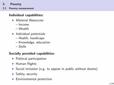
2. Poverty
2.2 Poverty measurement
Individual capabilities:
I Material Resources:– Income– Wealth
I Individual potentials:– Health, handicaps– Knowledge, education– Skills
Socially provided capabilities:
I Political participation
I Human Rights
I Social inclusion (e.g. to appear in public without shame)
I Safety, security
I Environmental protectionp.240
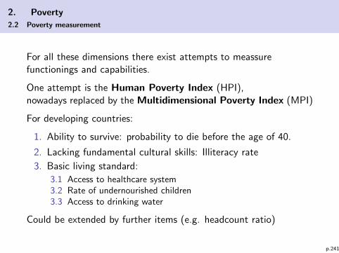
2. Poverty
2.2 Poverty measurement
For all these dimensions there exist attempts to meassurefunctionings and capabilities.
One attempt is the Human Poverty Index (HPI),nowadays replaced by the Multidimensional Poverty Index (MPI)
For developing countries:
1. Ability to survive: probability to die before the age of 40.
2. Lacking fundamental cultural skills: Illiteracy rate
3. Basic living standard:
3.1 Access to healthcare system3.2 Rate of undernourished children3.3 Access to drinking water
Could be extended by further items (e.g. headcount ratio)
p.241
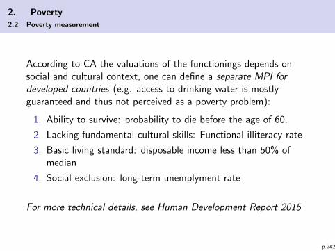
2. Poverty
2.2 Poverty measurement
According to CA the valuations of the functionings depends onsocial and cultural context, one can define a separate MPI fordeveloped countries (e.g. access to drinking water is mostlyguaranteed and thus not perceived as a poverty problem):
1. Ability to survive: probability to die before the age of 60.
2. Lacking fundamental cultural skills: Functional illiteracy rate
3. Basic living standard: disposable income less than 50% ofmedian
4. Social exclusion: long-term unemplyment rate
For more technical details, see Human Development Report 2015
p.242
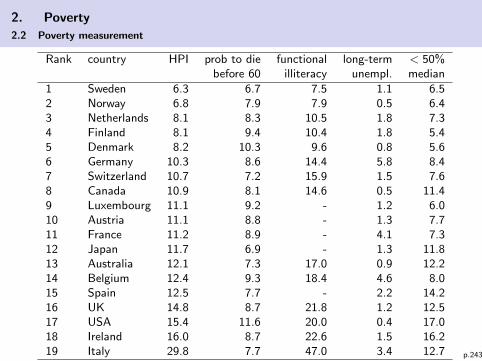
2. Poverty
2.2 Poverty measurement
Rank country HPI prob to die functional long-term < 50%before 60 illiteracy unempl. median
1 Sweden 6.3 6.7 7.5 1.1 6.52 Norway 6.8 7.9 7.9 0.5 6.43 Netherlands 8.1 8.3 10.5 1.8 7.34 Finland 8.1 9.4 10.4 1.8 5.45 Denmark 8.2 10.3 9.6 0.8 5.66 Germany 10.3 8.6 14.4 5.8 8.47 Switzerland 10.7 7.2 15.9 1.5 7.68 Canada 10.9 8.1 14.6 0.5 11.49 Luxembourg 11.1 9.2 - 1.2 6.010 Austria 11.1 8.8 - 1.3 7.711 France 11.2 8.9 - 4.1 7.312 Japan 11.7 6.9 - 1.3 11.813 Australia 12.1 7.3 17.0 0.9 12.214 Belgium 12.4 9.3 18.4 4.6 8.015 Spain 12.5 7.7 - 2.2 14.216 UK 14.8 8.7 21.8 1.2 12.517 USA 15.4 11.6 20.0 0.4 17.018 Ireland 16.0 8.7 22.6 1.5 16.219 Italy 29.8 7.7 47.0 3.4 12.7 p.243
2. Poverty
2.2 Poverty measurement
Global empirical picture:
I United Nations Millenium goals of poverty reduction:headcount ratio but also other (multidimensional) goals.
p.244
2. Poverty
2.2 Poverty measurement
Conflicting views:
I Poor countries suffer from natural conditions (e.g. climate),and colonial history.
I Strong correlation of poverty with political instability,corruption, and violence/war.
I “Development trap”: lack of infrastructure and humancapital ⇒ channeling aid from rich countries (globalresdistribution) might help to escape from development trap(e.g. Jeffrey Sachs).
p.245
2. Poverty
2.2 Poverty measurement
I However, empirical picture of developmemnt aid is ratherdisappointing (William Easterly). Success of aid stronglydepends on conditions (e.g. political institutions) andunderstanding of local customs. Aid could be even harmful.
I Danger of “learned poverty”: increased dependency on aidreduces capabilities and willingness of local authorities toimplement substantial reforms.
p.246

2. Poverty
2.2 Poverty measurement
I Counter position: don’t give aid but reform the system andopen the borders for trade and capital flows.
I So, does globalization reduce poverty?
⇒ Mixed empirical evidence. It also depends on the institutionalconditions (e.g. opening the borders for MNF with“resource-grabbing” strategies and repatriating the profits isless helpful; if benefits from globalization is extracted bycorrupt elites which are not re-invested, it is not helpful).
I Poverty due to war and natural catastrophees: aid is stillhelpful. But: capability approach reminds us to look for thespecific conditions of the people, their attitudes, values, andbehavior ⇒ deriving “mechanism design” from such microstudies (Angus Deaton, Esther Duflo).
p.247
2. Poverty
2.2 Poverty measurement
I No long-term solution without institutional reforms.Recall that political participation and freedom are mainingredients of the capability approach.
I Effective poverty reduction by migration of the poor(Angus Deaton, Paul Collier).
p.248