The Coe cient of Variation as a Measure of ... · The Coe cient of Variation as a Measure of Spectrophotometric Repeatability Paul Centore ... While the MCDM is suitable for practical

The Coefficient of Variation as a Measure ofSpectrophotometric Repeatability

Paul Centore

c© November 20, 2015

AbstractThe mean colour difference from the mean (MCDM) is a standard measure of

spectrophotometric repeatability. This paper proposes a supplementary measure: thecoefficient of variation (CoV), which is the ratio of the standard deviation of the mea-sured reflectances to their mean. The CoV is calculated from the same repeated samplemeasurements as the MCDM. Unlike the MCDM, the CoV depends only on physi-cal quantities, and not on perceptual quantities; furthermore, a CoV is defined foreach wavelength. This paper analyzes data from six different spectrophotometer-samplecombinations. An important empirical result is that the CoV is nearly constant acrosswavelengths, except when the reflectance at a particular wavelength is less than aboutfive percent, in which case measurement variability is dramatically greater. Since theMCDM tends to lose this fact through averaging, the CoV is recommended as an adjunctto the MCDM for spectrophotometer analysis and development. The CoV analysis alsoprovides evidence that samples’ surface geometry is a major factor in measurementvariability.

1 Introduction

Spectrophotometric repeatability1 means that repeated reflectance measurements of the samecolour sample, made by the same spectrophotometer, using the same protocol and condi-tions, should agree, even if the measurements are at different times. In practice, of course,agreement is not perfect. A standard metric of repeatability is the mean colour differencefrom the mean (MCDM). To calculate the MCDM for a particular colour sample, first makeN measurements of that sample’s reflectance spectrum. Next, calculate the mean reflectancespectrum. Choose an illuminant and observer2 with which to calculate the mean spectrum’scolorimetric coordinates. Similarly, calculate coordinates for each of the N original spec-tra. Then use an expression such as ∆E00 to find the colour differences between the meanspectrum and each of the N original spectra. The mean of these N colour differences is theMCDM. For colour practitioners, the MCDM provides an intuitive gauge of measurementvariability in a particular situation.

While the MCDM is suitable for practical situations, this paper proposes the coefficient ofvariation (CoV) as a supplementary repeatability metric, that provides a finer understand-ing in more analytical situations. Like the MCDM, the CoV is calculated from repeated

1

PAUL CENTORE

reflectance spectrum measurements of a particular colour sample. Unlike the MCDM, thereis a CoV for each wavelength λ. The mean reflectance for λ is the average of the individualreflectance measurements at λ. In addition, the sample standard deviation can be foundfor the reflectances at λ. The CoV for a probability distribution is defined as its standarddeviation, divided by its mean. We will use the following standard estimator3 for the CoVat λ :

CoV(λ) =

(1 +

1

4N

)sample standard deviation of reflectances at λ

average reflectance at λ. (1)

Leaving aside the technical distinction between an estimator and an underlying distribution,we will simply refer to Expression (1) as the CoV. For ease of understanding, this paper willexpress CoVs as percentages.

While the CoV gives a value at each wavelength, the MCDM gives one value for theentire visible spectrum. In effect, the MCDM, like the human visual system, integrates overall wavelengths to produce one answer. Integration can smooth over and obscure interestingfeatures that occur on a smaller scale. This paper will give some empirical instances in whichthe CoV reveals some important structure that the MCDM obscures. The most importantresult is the dramatically increased variability of spectrophotometric measurements whenreflectance is low, less than about 5%. Figure 1 shows an example that will be explainedin detail later. The vertical axis is the mean reflectance, for individual wavelengths, of theN measured reflectance spectra, and the horizontal axis is the CoV. The striking horizontalspike at the bottom indicates that spectrophotometric reliability degrades significantly atwavelengths where reflectance is very low.

Each reflectance on the vertical axis refers to one particular wavelength, so one dotmight give a CoV that occurs at, for example, 560 nm. A typical reflectance spectrumhas low reflectances for some wavelengths and high reflectances for others, and differentwavelengths can show different degrees of measurement variability. The MCDM produces asingle variability assessment by averaging out the very different contributions of the variouswavelengths. The CoV, on the other hand, considers wavelengths individually, and thuscaptures important information.

The CoV can also shed some light on the sources of measurement error. The magnitudeof measurement error depends on the spectrophotometer, the samples being measured, andthe measuring procedure. Empirical results will show that the CoV is largely wavelength-independent for a particular spectrophotometer-sample combination, except when a wave-length’s reflectance is very low. The sources of error are therefore also presumably wavelength-independent. Geometric effects, in which a sample’s surface structure causes a random se-quence of absorptions and reflections, are thus plausible candidates. The paper will showmathematically that geometric explanations are consistent with the observed CoV behavior.

The empirical data used in this paper consists of measurements from six different spectro-photometer-sample combinations. Two spectrophotometers were used: an X-Rite Color-Munki and an X-Rite i1Pro2. The samples cover various media (artist’s pastels, acrylicpaints, inkjet prints) and substrates (artist’s canvas, pastel paper, card stock). Each com-bination used somewhere between 24 and 65 samples, each of which was measured 10 or 12times. Repeatability is typically classified as short-term (on the order of seconds or min-utes), mid-term (on the order of hours or days), and long-term (on the order of weeks or

c© 2015 Paul Centore 2

THE COEFFICIENT OF VARIATION FOR SPECTROPHOTOMETRY

0

10

20

30

40

50

60

70

80

90

100

0 5 10 15 20 25 30 35

Mean R

efl

ecta

nce (

%)

Coefficient of Variation (%)

Figure 1: CoV vs Mean Reflectance for Case 4

longer). The data in this paper is all mid-term; the measurements for each combinationwere made within the span of a few hours. The mathematical analysis, however, would beidentical regardless of term, and there is no reason to expect different mathematical behaviorfor different terms. Repeated measurements are also typically classified as with replacement(the sample and spectrophotometer are physically separated after each measurement, andreunited for the next) or without replacement (the sample is not physically separated fromthe spectrophotometer between measurements). All the measurements in this paper werewith replacement.

The paper is organized as follows. First, the necessary mathematics behind the coefficientof variation is outlined. Next, the measurement experiments are described. Then, a visualexamination of some experimental data is used to motivate the CoV. The CoVs are calculatedfor the data and plotted. An analysis of wavelength-level data leads to the paper’s mainresult: the CoV indicates, much more clearly than the MCDM, that spectrophotometricmeasurements vary dramatically when reflectance is less than about 5%. Further wavelength-level analysis provides evidence for the hypothesis that samples’ surface geometry causesmuch of the observed variability. The CoV and MCDM are then compared, and appropriatesituations for the use of each measure are identified.

2 The Coefficient of Variation

The coefficient of variation (CoV) of a random variable is that variable’s standard deviation,divided by its mean. The CoV is conveniently expressed as a percentage. It can be thought

3 c© 2015 Paul Centore

PAUL CENTORE

of as a quantity’s expected variation, as a fraction of that quantity’s average value. TheCoV is useful when comparing quantities that differ by orders of magnitude. A classicalexample is comparing the length of mouse tails to the length of elephant tails: while themeans and standard deviations differ greatly, the CoV could plausibly be the same for both.In the current paper, the random variable of interest will be the reflectance measurementsof surface colours. Reflectances can typically vary by about two orders of magnitude, fromlows just under 1% to highs that are over 90%. Despite this wide set of values, we will seethat the CoV of reflectance measurements is nearly constant, except when reflectances arebelow about 5%.

The term coefficient of variation, like the term standard deviation, is often applied intwo distinct contexts, population statistics and sample statistics, without making the dis-tinction explicit. Population statistics assumes that a probability distribution of interest isknown completely. If the distribution only takes on N discrete values xi, then its populationstandard deviation σP is given by

σP =

√√√√ 1

N

N∑i=1

(xi − µ)2, (2)

where µ is the mean value:

µ =1

N

N∑i=1

xi. (3)

Unlike population statistics, sample statistics does not assume that a distribution isknown. Instead, there is a set of samples, or measurements, from an underlying but unknowndistribution. Summary quantities like the population standard deviation are still of interest,but can only be estimated from a sample. The sample standard deviation σ is given by

σ =

√√√√ 1

N − 1

N∑i=1

(xi − µ)2. (4)

Apart from the denominator N − 1 versus the denominator N, the expressions for the pop-ulation and sample standard deviations are identical. The denominator adjustment insuresthat the expected value of the sample standard deviation is in fact the population standarddeviation.4 An estimator for a quantity, whose expected value is that quantity, is said tobe unbiased, so the sample standard deviation is an unbiased estimator for the populationstandard deviation. The distinction between populations and samples is often not made,or only made implicitly. Frequently Equation (4) is referred to as the standard deviation,because, in most practical situations, only measured samples are available. In fact, however,Equation (4) is only an estimator.

Unlike the standard deviation and the mean, no general unbiased estimator is known forthe coefficient of variation. One common estimator,3 which will be used in this paper, is

CoV =

(1 +

1

4N

)σ

µ. (5)



This estimator is generally considered adequate when the underlying population follows anormal distribution.

In spectrophotometry, a practitioner is interested in the reflectance ρ(λ) of a sampleat a wavelength λ. While the reflectance itself is presumably an unvarying number, spec-trophotometric measurement is a random process, so the reflectance measurements follow aprobability distribution. A calibrated spectrophotometer is usually unbiased, meaning thatthe expected value of its measurements is the true reflectance. Furthermore, even thoughthe measurements have some spread, they tend to cluster symmetrically around their ex-pected value. These properties make a normal distribution a reasonable approximation tothe distribution of reflectance measurements. Equation (5) is then a reasonable estimator ofthe population CoV, which is the rationale for using it here.

A naive estimation approach would simply have divided the sample standard deviationby the sample mean, giving

CoV =σ

µ. (6)

Equation (6) is just Equation (5) with a coefficient of 1 instead of the coefficient 1 + 1/(4N).In practice, the adjustment of 1/(4N) is usually inconsequential. With ten measurementsfor example, 1/(4N) is only 0.025, so the coefficient in Equation (5) is 1.025 instead of 1,a difference of just 2.5 percent. As the number of measurements increases, 1/(4N) goesto 0 asymptotically, so its influence is even smaller. The choice between the estimators inEquations (5) and (6) is therefore not of much import.

3 Measurement Data

3.1 Experiments

This paper’s conclusions about the CoV are based on reflectance measurements from sixdifferent combinations of spectrophotometers and samples. Only two combinations weremeasured specifically for this paper; the rest were measured in the course of other projects.In fact, the idea of using the CoV as a repeatability metric arose while calculating MCDMsfrom these measurements: a close look at wavelength-level data revealed some regularitiesthat the MCDM was overlooking.

Table 1 lists the spectrophotometers and samples. In Cases 2 and 3, the X-Rite Color-Munki and X-Rite i1Pro2 measured the same chart. The two devices were alternated (first24 measurements by the ColorMunki, then 24 by the i1Pro2, then 24 by the ColorMunki,and so on), to make the comparisons as similar as possible. Cases 4 and 5 used differentselections of paint samples. In both cases, the paints were mixtures of Golden acrylic paints,along with a few paints straight from the tube. The data sets in general are from differ-ent projects, so contain different colours. In all six cases, however, the samples spanneda wide gamut of hues, values, and chromas, to avoid biases. Both spectrophotometers usea 45◦/0◦ measuring geometry, but the i1Pro2 uses ring illumination while the ColorMunkiuses unidirectional illumination. The i1Pro2 offers a choice of measurement conditions; in allcases, M2 (UV excluded filter) was selected. All the measurements were with replacement:


PAUL CENTORE

Device Description of Samples Number Measurements Mean Medianof Samples of Each Sample MCDM CoV (%)

1 i1Pro2 Coated GoeGuide samples 65 10 0.15 0.57from Pantone fan deck

2 ColorMunki ColorChecker reproduction, 24 12 0.19 1.04printed on Kirkland Signature paper

3 i1Pro2 ColorChecker reproduction, 24 12 0.27 1.24printed on Kirkland Signature paper

4 ColorMunki Golden Acrylics, applied by 56 10 0.34 2.03handheld brush on Dick Blick canvas

5 i1Pro2 Golden Acrylics, applied by 65 10 0.38 2.01handheld brush on Dick Blick canvas

6 i1Pro2 Sennelier pastels, applied by hand 56 10 1.03 5.38on Somerset Radiant White paper

Table 1: Measurement Experiments

the spectrophotometer and sample were physically separated between measurements, andreunited for each measurement. The measurements for each case were all completed withinthe span of a few hours, so these are mid-term repeatability studies.

The second last column in Table 1 reports the mean MCDM. For any one case, eachsample has a mean measured reflectance spectrum. The first case, for example, has 65mean spectra, each an average of 10 individually measured spectra. Each sample in thefirst case produces 10 colour differences; each difference is between the mean spectrum andone measured spectrum. All colour differences were calculated with the ∆E00 expression,2,5

assuming Illuminant C and the 1931 Standard Observer. The average of these 10 colourdifferences is the MCDM for that sample, so there are 65 MCDMs. The mean MCDMshown in the table is the average of the 65 MCDMs. Details of the CoV entries in the lastcolumn will be given later.

The MCDM entries can be compared with some previous work. Wyble and Rich6,7

earlier attained mid-term MCDMs of between 0.10 and 0.27 (see Table II of Ref. 6) for fourhandheld spectrophotometers (the i1Pro2 and the ColorMunki are both handheld) whenmeasuring disks of pressed polytetrafluoroethylene (PTFE). These disks are more similar tothe first three cases in Table 1 than the last three cases. Since the first three cases foundmean MCDMs of between 0.15 and 0.27, the results presented here are on par with theirresults, providing a sanity check.

3.2 Coefficient of Variation Calculations

The CoV was motivated by a visual examination of the measured reflectance spectra. Asan example, Figure 2 shows all 10 reflectance measurements for Case 5, for the first of the65 samples. The i1Pro2 returned reflectance measurements at wavelengths between 380and 730 nm, in increments of 10 nm. Figure 2 shows the measured spectra as solid lines,while Figure 3 shows them more suggestively as isolated data points. Over the wavelength600 nm, for example, there are 10 reflectance percentages, one for each spectrophotometricmeasurement of the sample. The spread in these ten percentages can be estimated visually



0

20

40

60

80

100

300 400 500 600 700 800

Ref

lect

ance

(%

)

Wavelength (nm)

Figure 2: Measured Reflectance Spectra of First Sample in Case 5, as Lines

from the vertical extent of the data. In this example, the higher reflectances, at the right ofthe plot, have a greater vertical extent than the lower reflectances, at the left of the plot.

This observation motivates the CoV. The reflectance at a particular wavelength is bestestimated by averaging the repeated reflectance measurements at that wavelength; theseaverages, of course, yield the mean reflectance spectrum. The spread of the reflectances ata particular wavelength is estimated by the sample standard deviation of those reflectances.Visually, it seems that higher reflectances show greater spread, so one naturally hypothesizesthat the spread is a constant fraction of the mean. From the mathematical discussion, theCoV is just this fraction, i.e. the standard deviation divided by the mean. Figure 4 plotsthese CoVs as percentages, for the data in Figure 3.

With the exception of the endpoints (where measurements are likely unreliable), theCoVs are fairly consistent across wavelengths, at slightly over 1 percent. For many centrallyclustering distributions, such as occur with repeated measurements, nearly all observed val-ues are within three standard deviations of the mean. If the mean is 50 percent (as occursat 410 nm), and the CoV is 1 percent, then the standard deviation is 0.5 percent (that is,1 percent of 50 percent), so almost all the observed values would fall between 48.5 and 51.5percent. With a mean of 80 percent (as occurs in the right half of the plot) and the sameCoV, the observed values would fall between 77.6 and 82.4 percent. The total spread is 3percentage points at 50 percent, and 5 percentage points at 80 percent. These predictionsare consistent with Figure 3.

Once this example and many similar ones validated the CoV as a measure of spectropho-tometric repeatability, CoVs were calculated for each sample, at each wavelength, in eachof the six cases in Table 1. Figures 5 through 10 plot the CoVs. In each figure, all the


PAUL CENTORE

0

20

40

60

80

100

300 400 500 600 700 800

Ref

lect

ance

(%

)

Wavelength (nm)

Figure 3: Measured Reflectance Spectra of First Sample in Case 5, as Points

0

1

2

3

4

5

300 400 500 600 700 800

Co

effi

cien

t o

f V

aria

tio

n (

%)

Wavelength (nm)

Figure 4: Coefficients of Variation for First Sample in Case 5



0

5

10

15

20

25

350 400 450 500 550 600 650 700 750

Coef

fici

ent

of

Var

iati

on

(%

)

Wavelength (nm)

Figure 5: Coefficients of Variation for Case 1 (GOE Guide Measured with i1Pro2)

CoVs from one sample are plotted as a solid line that spans all the measured wavelengths.The total number of CoVs in each figure is the number of samples times the number ofwavelengths. For each figure, the median of the set of all CoVs was calculated. This medianappears in the last column of Table 1.

4 Analysis

4.1 Wavelength-Independence

The CoVs in Figures 5 through 10 tend to cluster. In Figure 8, for example, the bulk of the56 samples cluster near 1%. Perhaps 10 to 15 samples are noticeably outside this clustering;without those samples, all the plots would form one thick line. (A later section will explainthe samples outside the cluster in terms of low reflectance.) The important observation hereis that, for any one case, the CoV only depends minimally on the wavelength. Given that,the median CoV in Table 1, even though it was calculated over data from all 36 wavelengths,would apply equally well to any one wavelength. In fact, the median was chosen over themean because of robustness—the small percentage of outliers will not change the median’svalue, even if the outliers are very large. As a result, the median accurately captures thevalue which the CoVs cluster around.

Though the CoV does not depend significantly on wavelength, it does vary significantlyfrom case to case. Table 1 shows that CoVs span an order of magnitude over the six cases.Since behavior at different wavelengths is not a factor, there must be other factors, and those


PAUL CENTORE

0

5

10

15

20

25

350 400 450 500 550 600 650 700 750

Coef

fici

ent

of

Var

iati

on

(%

)

Wavelength (nm)

Figure 6: Coefficients of Variation for Case 2 (ColorChecker Measured with ColorMunki)

0

5

10

15

20

25

350 400 450 500 550 600 650 700 750

Co

effi

cien

t o

f V

aria

tio

n (

%)

Wavelength (nm)

Figure 7: Coefficients of Variation for Case 3 (ColorChecker Measured with i1Pro2)



0

5

10

15

20

25

350 400 450 500 550 600 650 700 750

Coef

fici

ent

of

Var

iati

on

(%

)

Wavelength (nm)

Figure 8: Coefficients of Variation for Case 4 (Acrylic Paints Measured with ColorMunki)

0

5

10

15

20

25

350 400 450 500 550 600 650 700 750

Co

effi

cien

t o

f V

aria

tio

n (

%)

Wavelength (nm)

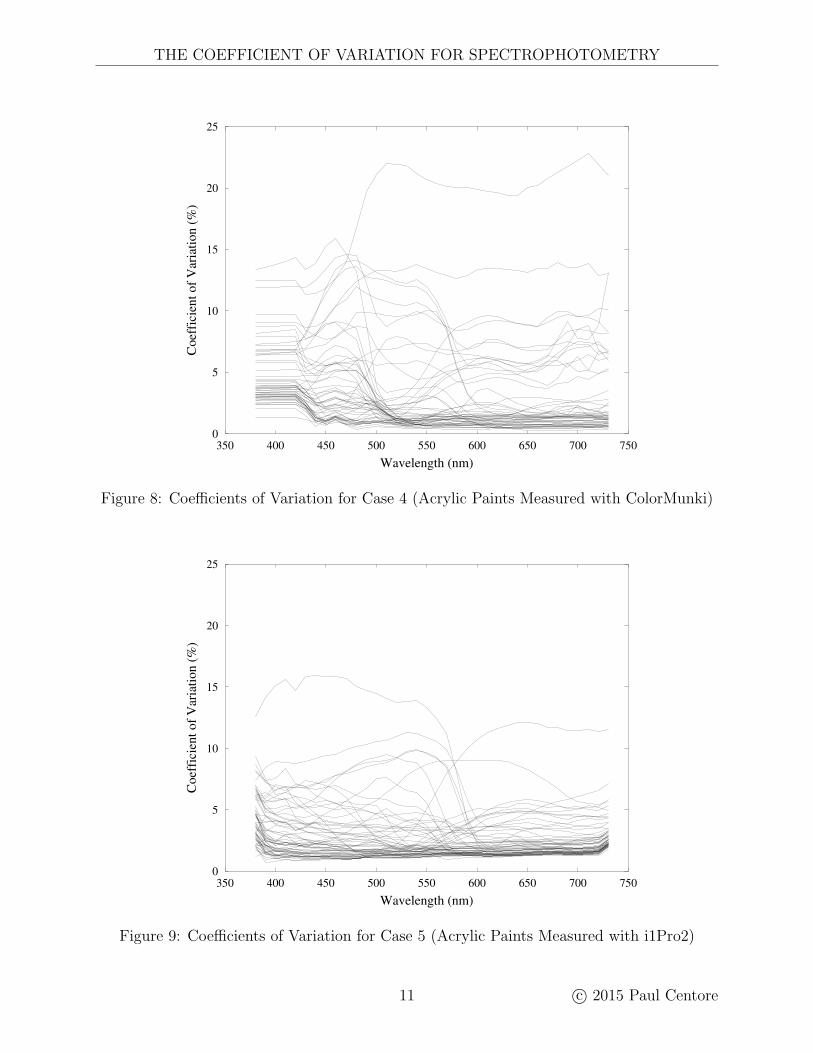
Figure 9: Coefficients of Variation for Case 5 (Acrylic Paints Measured with i1Pro2)


PAUL CENTORE

0

5

10

15

20

25

350 400 450 500 550 600 650 700 750

Coef

fici

ent

of

Var

iati

on

(%

)

Wavelength (nm)

Figure 10: Coefficients of Variation for Case 6 (Sennelier Pastels Measured with i1Pro2)

other factors must be independent of wavelength. A later section will make the case thatsurface geometry is such a factor.

4.2 Low Reflectances

A closer look at the 10 to 15 outlying CoV curves in Figure 8 revealed an interesting feature:the high CoVs seen there are physically correlated with low reflectances. Figure 1 plots theCoV against the mean reflectance for all the samples and wavelengths in Figure 8. Eachpoint refers to a particular sample and wavelength; for example, one point is the resultsfor the 17th sample at wavelength 470 nm. There are 56 samples in Case 4, and each ismeasured at 36 wavelengths, so Figure 1 contains 2016 points in all. The figure shows thathigh variability occurs only when the reflectance is below about 5%, and that the variabilityincreases dramatically there. Furthermore, the variability in CoV appears nearly constantwhen reflectances are between 5% and 90%. If reflectances below a few percent were removedfrom Figure 8, the plot would collapse to a fairly compact thick line. A low reflectance istherefore nearly a perfect predictor of a high CoV. In any event, the sudden spike in CoVseen in Figure 1 as reflectances approach 0 is too striking to ignore.

Perceptually, low reflectances correspond to dark colours. In fact, the prominent upperline in Figure 8, with CoVs hovering around 20 percent, is a very dark blue, almost black.The other isolated lines in the figure are also dark colours. This relationship explains adiscrepancy in the figures: Figures 5 through 7 show few isolated lines, while isolated linesare plentiful in Figures 8 through 10. The last three figures consisted of artist’s pastelsand artist’s acrylic paints, and presented a wide range of colours, including some very dark



0

10

20

30

40

50

60

70

80

90

100

0 5 10 15 20 25 30 35

Mean

Refl

ecta

nce (

%)


Figure 11: CoV vs Mean Reflectance for All Cases

colours. The second and third figures consist of measurements of a ColorChecker reproduc-tion, which contains some darker colours, but not the extreme darks seen in the last threecases. Finally, the selection of colours from the GoeGuide were taken from a “Summer”fashion palette, with a paucity of dark colours. Had the first three cases contained somevery dark colours, then they would likely have also exhibited the CoV outliers seen in thelast three cases.

To make sure that Case 4 is not an anomaly, Figure 1 was augmented to include a pointfor every sample, at every wavelength, in all six cases, for a total of 10,440 points. Figure 11shows the result. Visually, the same prominent spike appears along the bottom, indicatingthat the correspondence of high CoVs and low reflectances occurred consistently.

A random additive noise factor partially explains the results in Figure 11, but other fac-tors are needed, too. Suppose that the spectrophotometer was unbiased at each wavelength,and its measurement error was an unbiased normal distribution with a standard deviation σ.σ would be measured in percentage points, and, because it is additive, σ would be the sameat all reflectances, high or low. Figure 12 shows the CoVs, as functions of reflectances, thatwould result if measurement variability was due to additive noise alone. Curves are drawnfor σ’s from 1% down to 0.01%. A horizontal line at 5% reflectance is shown, for comparisonwith Figure 11.

Additive noise by itself would cause a spike at low reflectances, as Figure 12 shows. Ifadditive noise were the only error, then all the data in Figure 11 would fall along one of thecurves in Figure 12. The strong vertical column in Figure 11, however, when the CoV is justover 5%, falsifies this possibility. While the curves in Figure 12 could explain much of thebehavior seen in Figure 11, it is also clear that other factors must be at work.


PAUL CENTORE

0

20

40

60

80

100

0 5 10 15 20 25 30 35


Refl

ecta

nce (

%)

5

1.00%

0.50%

0.25%

0.10%

0.01%

Figure 12: CoV vs Reflectance, When the Only Measurement Error is Additive Noise

4.3 Surface Geometry

The CoVs in Table 1 span an order of magnitude, from 0.57 to 5.38. Since CoVs arelargely wavelength-independent, any explanation for this wide span must also be wavelength-independent. One natural explanation is the samples’ texture or surface structure. Theartist’s pastels in Case 6, in particular, are very dusty. They were applied to the paper byrubbing the pastel over a square area, and then smoothing with a finger. A cloud of particlescan easily be produced by shaking the samples or blowing on them. Glossy samples, suchas the printed ColorChecker and coated GoeGuides, produced the lowest CoVs, while theslightly bumpy canvas texture produced intermediate CoVs. This section shows that surfacegeometry is a plausible explanation for the wide span of CoVs, and is consistent with theobserved wavelength-independence.

Roughly speaking, spectrophotometric measurement error originates from three sources:the spectrophotometric device, the samples, or the measurement protocol. The six casesoffer some controlled experiments, in which only one factor is varied. These experimentswill allow us to conclude that the second source, sample irregularity, is causing most of thewide CoV span. The first source of error, the spectrophotometers, can easily be eliminated:Cases 1, 2, 5, and 6 all involve an i1Pro2 spectrophotometer (in fact, the very same physicaldevice), yet yield very different CoVs. Since instrument instability would have made allthe CoVs uniformly high, the instrument itself must be reasonably stable. A cross-modelcomparison is also avaiable. In Cases 2 and 3, the i1Pro2 and ColorMunki measured thesame set of samples, and gave similar CoVs of 1.04 and 1.24. In Cases 4 and 5, the i1Pro2and the ColorMunki again measured similar (though not identical) samples, giving CoVs of



2.01 and 2.03. Since these differences are not large, we can eliminate the first source of error.Since the measuring protocol was identical for all spectrophotometers and samples, the thirdsource of error, measuring protocol, can also be eliminated.

The remaining source of error is then the samples themselves, and wavelength-indepen-dence suggests their geometric surface structure as a plausible explanation. The rationale isthat an irregular surface leads to randomness in the number of times α that an incoming lightray interacts with the sample, and that this randomness explains CoV variability. At eachinteraction, some percentage pA of light will be absorbed, and the rest will be scattered. Thetotal percentage of absorbed light would then be a function not only of pA, but also of therandom variable α. If irregular geometry makes α highly variable, then the total absorptionpercentage is also highly variable. The percentage of light that is absorbed or scattered ateach interaction is a function of wavelength, but α is not a function of wavelength.

The interaction sequence would be shorter for smooth surfaces and longer for unevensurfaces. A light source would interact only once with a perfectly smooth sample. Somelight would be absorbed, and some would be scattered, either as a first-surface reflectioncomponent or as a diffuse, approximately Lambertian, component. The scattered light wouldnot re-enter the sample, so there would only be a single interaction. The smooth surfacesin Cases 1 through 3 likely produce such short interaction sequences, and all produce lowerCoVs. Now suppose that the sample’s texture is not smooth. Perhaps, like the Torrance-Sparrow model,8 it contains microscopic specular facets at various orientations. It couldbe even more complicated: given the pastel samples’ dustiness, some pastel particles couldbe lying on the surface. With such uneven textures, scattered light could re-interact withthe sample, likely multiple times. This long sequence would cause α to be high, and, moreimportantly, to be highly variable. As a result, CoV would be consistently high, as it isin Case 6. The interaction sequence would also be independent of wavelength, so the CoVwould be the same at all wavelengths, as we observed.

4.4 Comparison of CoV and MCDM

The MCDM is already a standard measure for spectrophotometric repeatability, while theCoV is a proposed measure. This section compares and contrasts the two measures, andconcludes that the CoV can be a helpful supplement to the MCDM, especially in analysisand research.

Both measures quantify the variability seen in spectrophotometric observations, and thetwo measures correlate well. The last two columns of Table 1 list the CoVs and MCDMs forthe six cases studied. With the exception of the transposition of two nearly equal numbers,both quantities are listed in ascending order. The conclusion is that CoV tends to increasewhen MCDM increases, and vice versa. Either measure, then, gives an estimate of repeata-bility. The MCDM, however, uses the familiar DE scale, making it easy for a practitioner tograsp the result perceptually, and to estimate its effect in a certain situation. This ease ofinterpretation recommends the MCDM for practical situations

In scientific situations, on the other hand, the MCDM has some shortcomings. First, itconflates data from different wavelengths. Second, it requires a choice of illuminant. Third,it uses non-physical quantities such as a colour difference expression. From a practical pointof view, of course, these shortcomings are strengths, because they account for perceptual


PAUL CENTORE

0

10

20

30

40

50

60

70

80

90

100

0.0 0.5 1.0 1.5 2.0

Y (

C/2

)

MCDM (C/2)

Figure 13: MCDM vs CIE Y for All Cases

factors: human vision also averages across wavelengths and assesses colour differences. Themain disadvantage of accounting for perceptual factors is that valuable analytic and engi-neering knowledge is overlooked.

As an example, let us recalculate the plot in Figure 11, using perceptual quantities insteadof physical quantities. In particular, we will replace the CoV (on the horizontal axis) withthe MCDM. A perceptual correlate of reflectance (on the vertical axis) is CIE lightness Y,which is calculated from the photopic luminous efficiency function.9 Y takes values from0 to 100. A value of Y of 10 corresponds approximately to a Munsell value of 1, whichwould result from an ideal grey whose reflectance is 1% at every visible wavelength. Y wascalculated for all 290 samples in the six cases. Each sample also had an associated MCDM.Both Y and the MCDM require an illuminant and an observer.2 For consistency, IlluminantC and the 1931 2◦ standard observer were used for all calculations. The resulting scatterplotin Figure 13 is a perceptual analogue of the physical data in Figure 11.

While Figure 13 lacks the obvious spike seen at the bottom of Figure 11, the samerelationship is present in a muted form. Most of the MCDMs above 0.5 occur when Y isless than 20 percent, which corresponds to a reflectance well below 5 percent, and only a fewoccur when Y is above 50 percent, which corresponds to a reflectance just below 20 percent.Figures 11 and 13 therefore exhibit the same trend, though it is not as pronounced in Figure13.

Without the benefit of Figure 11, though, the trend in Figure 13 would likely be missed.While sophisticated statistical tests might reveal that some relationship is present, likely noengineer or analyst would think to apply such tests, because they would not observe thephenomenon being tested for. Even if a statistically significant relationship were found, it



would likely be dismissed as unimportant. For engineers in particular, the CoVs in Figure11, even without any statistical analysis, make it clear that development effort should bedirected to low reflectances. Furthermore, test samples can be obtained easily, because thesamples only need low reflectances at a few wavelengths; without this insight, much timecould be wasted looking for very black samples that have low reflectances across the entirevisible spectrum. Once samples are chosen, engineering improvements to spectrophotometerscan be easily evaluated, using plots like Figure 11.

The CoV is also more useful than the MCDM when analyzing bi-directional reflectancedistribution functions (BRDFs) for semi-reflective surfaces. Rather than measuring oneoverall reflectance curve, the BRDF measures a reflectance curve for each pair of directions.The first direction in the pair specifies the ray (in three-dimensional space) followed by lightimpinging on the sample, and the second direction specifies the ray along which reflectedlight leaves the sample. The BRDF is useful for glossy or semi-reflective surfaces, where theexiting light is a mixture of spectrally reflected incoming light (which could be of any colour)and the surface’s local colour. For a pair of directions in which gloss is a factor, the MCDMcan be determined but is not very informative because it is not clear what the “true” colourshould be. The CoV, on the other hand, which only looks at individual wavelengths, doesnot require a true colour to estimate measurement variability.

A major analytic benefit of the CoV over the MCDM, then, is that the CoV providesfiner physical information about the measurement process, and the factors that influencespectrophotometric variability. For this reason, analysis and research should use not just theMCDM, but also the CoV.

5 Summary

This paper has proposed the coefficient of variation (CoV) as a supplementary measure ofspectrophotometric repeatability, at least for analysis and development; the long-establishedmean colour difference from the mean (MCDM) is likely more suitable for practical appli-cations. A set of 290 colours, of various media and substrates, measured with two differentspectrophotometers, provided data on which the paper’s conclusions are based.

A major empirical result was that the CoV for a particular kind of sample and spec-trophotometer was nearly constant across all wavelengths, except when the reflectance atthat wavelength when less than about 5%. When reflectances were very low, the CoVincreased dramatically. Furthermore, dramatic increases were always associated with lowreflectances, suggesting that we have isolated the problematic conditions for measurementvariability. While a particular spectrophotometer-sample combination would have the sameCoV for all wavelengths, a different combination could have a different CoV; the CoVs in thedata set, in fact, spanned an order of magnitude. The samples ranged from glossy, printedcolours to dusty artist’s pastels, and the more uneven the surface, the higher the CoV. Fromthis correlation, combined with the CoV’s wavelength-independence, it was inferred thatsamples’ surface geometric structure explained much of the observed spectrophotometricmeasurement variability.


PAUL CENTORE

References

1. Roy S. Berns, Billmeyer and Saltzman’s Principles of Color Technology, 3rd ed., JohnWiley & Sons, 2000.

2. CIE, Colorimetry, 3rd ed., CIE Publication No. 15:2004, Vienna, 2004.

3. Robert R. Sokal, F. James Rohlf, Biometry: The Principles and Practice of Statistics inBiological Research, 4th ed., W. H. Freeman and Company, 2012.

4. Dennis D. Wackerly, William Mendenhall III, & Richard L. Scheaffer, MathematicalStatistics with Applications, 5th ed., Duxbury Press, 1996.

5. Gaurav Sharma, Wencheng Wu, & Edul N. Dalal, “The CIEDE2000 Formula: Imple-mentation Notes, Supplementary Test Data, and Mathematical Observations,” Color Re-search and Application, Vol. 30, Number 1, February 2005, pp. 21-30.

6. David R. Wyble & Danny C. Rich, “Evaluation of Methods for Verifying the Performanceof Color-Measuring Instruments. Part I: Repeatability,” Color Research & Application,Vol. 32, No. 3, pp. 166-175, June 2007.

7. David R. Wyble & Danny C. Rich, “Evaluation of Methods for Verifying the Performanceof Color-Measuring Instruments. Part II: Inter-Instrument Reproducibility,” Color Re-search & Application, Vol. 32, No. 3, pp. 176-194, June 2007.

8. K. E. Torrance & E. M. Sparrow, “Theory for Off-Specular Reflection From RoughenedSurfaces,” JOSA, Vol. 57, No. 9, pp. 1105-1114, September 1967.

9. G. Wyszecki and W. S. Stiles, Color Science: Concepts and Methods, Quantitative Dataand Formulae, 2nd ed., John Wiley & Sons, 1982.


Documents

The Coe cient of Variation as a Measure of ... · The Coe cient of Variation as a Measure of Spectrophotometric Repeatability Paul Centore ... While the MCDM is suitable for practical