Embed Size (px)
Citation preview

International capital �ows and global imbalances
Sewon Hur
University of Pittsburgh
March 3, 2015
International Finance (Sewon Hur) Lecture 4 March 3, 2015 1 / 38
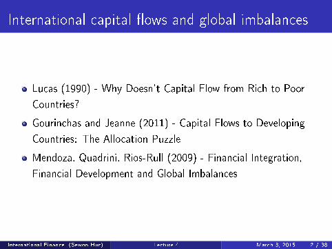
International capital �ows and global imbalances
Lucas (1990) - Why Doesn't Capital Flow from Rich to Poor
Countries?
Gourinchas and Jeanne (2011) - Capital Flows to Developing
Countries: The Allocation Puzzle
Mendoza, Quadrini, Rios-Rull (2009) - Financial Integration,
Financial Development and Global Imbalances
International Finance (Sewon Hur) Lecture 4 March 3, 2015 2 / 38

Gourinchas and Jeanne (2011)
The basic neoclassical growth model predicts that countries that
enjoy higher productivity growth should receive more net capital
in�ows. This is not true in the data.
AGO
ARG
BEN
BGD
BOL
BRA
BWA
CHL
CHN
CIV
CMR
COG
COL
CRICYP
DOMECU
EGYETH
FJI
GAB
GHAGTM
HKG
HND
HTI
IDN IND
IRN
ISR
JAM
JOR KEN
LKA
MARMEX
MLI
MOZ
MUS
MWI
MYS
NER
NGA
NPL
PAK
PAN
PER
PHLPNG
PRYRWA
SEN
SGP
SLV
SYR
TGO
THA
TTO
TUN
TUR
TWN
TZA
UGA
URY
VEN
ZAF KOR
MDG
−10
−5
05
10
15
Cap
ita
l In
flo
ws (
perc
en
t of
GD
P)
−4 −2 0 2 4 6Productivity Growth (%)
Figure 1: Average productivity growth and average capital inflows between 1980 and 2000.
wedge that distorts investment decisions, and one wedge that distorts saving decisions. It isthen possible, for each country in our sample, to estimate the saving and investment wedgesthat are required to explain the observed levels of savings and investment (and thereforeof net capital flows). We find that the investment wedge cannot, by itself, explain theallocation puzzle, and that solving the allocation puzzle requires a saving wedge that isstrongly negatively correlated with productivity growth. That is, the allocation puzzle is asaving puzzle.
We then look at a decomposition of international capital flows into public and privateflows, similar to Aguiar and Amador (2011). We confirm that paper’s finding that the alloca-tion puzzle is mostly a feature of public flows, and in addition find that the accumulation ofinternational reserves plays a role in generating the puzzle. However, we do not find robustevidence that private flows conform to the predictions of theory.
What can explain this puzzling allocation of capital flows across developing countries?Our wedge analysis shows that the explanation must involve the relationship between savingsand growth, and our flow decomposition suggests that reserve accumulation plays an impor-tant role. This suggests to us that the solution to the allocation puzzle should be lookedfor at the nexus between growth, saving, and reserve accumulation. Why do countries thatgrow more also accumulate more reserves, and why is this reserve accumulation not offsetby capital inflows to the private sector? We discuss possible explanations at the end of thepaper—some of which were developed since the first version of this paper was circulated. Noattempt is made to discriminate empirically between these explanations —the objective ofthe last section of the paper being to propose a road map for future research rather than toestablish new results.
This paper lies at the confluence of different lines of literature. First, it is related to the
2
International Finance (Sewon Hur) Lecture 4 March 3, 2015 3 / 38

Model
Small open economy that can borrow and lend at world interest
rate R∗
Time is discrete and there is no uncertainty
Technology: Yt = Kαt (AtLt)
1−α
Labor supply is exogenous, equal to the population Lt = Nt
Resource constraint:
Ct + It + R∗D = Yt + Dt+1
It = Kt+1 − (1− δ)Kt
Country's external debt Dt
International Finance (Sewon Hur) Lecture 4 March 3, 2015 4 / 38

Model
Capital in�ows Dt+1 − Dt is equal to domestic investment It
minus savings St = Yt − (R∗ − 1)Dt − Ct
Rt = α(kt/At)α−1 + 1− δ where kt = Kt/Nt
Since Rt = R∗ in equilibrium,
kt = k∗ ≡(
α
R∗ + δ − 1
)1/(1−α)
where k = k/A (capital stock per e�cient unit of labor)
International Finance (Sewon Hur) Lecture 4 March 3, 2015 5 / 38

Model
Exogenous, deterministic productivity path, {At}t=0,..∞,
At ≤ A∗t = A∗0 (g ∗)t
where g ∗ − 1 is the growth rate of the world technology frontier
Gap between domestic productivity and the productivity with no
�catch-up�
πt ≡At
A0 (g ∗)t− 1
Growth rate always converges to g ∗ , and π ≡ limt→∞ πt is
well-de�ned.
International Finance (Sewon Hur) Lecture 4 March 3, 2015 6 / 38

Model
Representative household solves
max∞∑
s=0
βsu(ct+s)
s.t. Ct + Kt+1 ≤ R∗Kt + (Dt+1 − R∗Dt) + wtNt
where u(c) = log(c), wt = (1− α)kαt A1−αt
Euler equation
1
ct= βR∗
1
ct+1
Assume R∗ =g ∗
β, which holds if ROW is composed of developed
economies that have the same preferences and are in steady
state BGP.International Finance (Sewon Hur) Lecture 4 March 3, 2015 7 / 38

Capital Flows and Productivity Catch-Up
1 If k0 = k∗ (optimal initial capital) and d0 = 0 (no initial debt),
then the country receives positive net capital in�ows i� π > 0.
Capital �ows into the developing countries whose TFP catches
up relative to the world frontier, and �ows out of the countries
whose TFP falls behind.
2 If identical except for long-run productivity catch-up, then
country A receives more capital in�ows i� it catches up more
than country B, i.e. πA > πB .
Other things equal, countries that grow faster should receive
more capital �ows.
The opposite is true in the data, hence the puzzle.
International Finance (Sewon Hur) Lecture 4 March 3, 2015 8 / 38
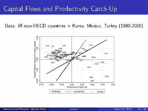
Capital Flows and Productivity Catch-Up
Data: 65 non-OECD countries + Korea, Mexico, Turkey (1980-2000)
KOR
TWN
BGD
HKG
PNG
CHN
IDNPHL
SGP
LKA
PAK
FJI INDTUR
MYS
THANPL
BOL
PAN
VEN
HTI
COLPRYCRIMEXSLVTTO
PER
ARG
URYBRAGTM DOM
JAM
HNDECU
CHL
ISRBEN
NGA
MOZ
TGO
TZAJOR
CIV
MAR MUSIRN
MLI
COG
SYRZAF
NER MWIGHA
RWA
AGOSEN
KEN
MDG UGA
BWA
TUN CYP
ETHGAB EGY
CMR
-2.0
0-1
.00
0.00
1.00
2.00
Capi
tal I
nflow
s (re
lativ
e to
initia
l out
put)
-0.75 -0.50 -0.25 0.00 0.25 0.50 0.75 1.00Productivity Catch-Up
Predicted: investment saving
Figure 2: Productivity catch-up (π) and change in external debt (∆D/Y0) together withpredicted investment
(∆DI/Y0
)and predicted saving
(∆DS/Y0
)terms.
significant at the 1 percent level.21
In addition to confirming, with different measures, the basic correlation already shownin Figure 1, Figure 2 compares the data to the prediction of the basic neoclassical growthframework. We observe that capital flows are not only negatively correlated with the modelpredictions but also tend to be smaller in absolute value. This is especially true if we look atthe saving component, which implies that a one percentage point increase in the productivitycatch-up variable π should raise capital inflows by 5.25 percent of initial output.22 For acountry such as Korea, with a productivity catch up π equal to 0.61, the model predictsinvestment and saving components of net capital inflows each in excess of 130 percent ofinitial output. Conversely, for Madagascar, with a relative productivity decline π equal to-0.47, the model predicts investment and saving components of net capital outflows each inexcess of 100 percent of initial output!
As noted at the end of section 2, the saving component is very responsive to growth in themodel because of the assumption that consumers are infinitely-lived and can perfectly smoothconsumption. Introducing financial frictions or assuming different preference structures couldreduce significantly the importance of the saving component.23 By contrast, observed flows
21The slope of the regression line in figure 2 is -0.68 with a s.e. of 0.18 (p-value smaller than 0.01).22The slope of the investment term ∆Di/Y0 is (ng∗)20 = 2.14 while the slope of the saving term ∆Ds/Y0
is (1 + (1− α)k∗(α−1)/R∗∑19t=0 (ng∗)t (1− t/20) (ng∗)20 = 5.25.
23In the limit case where households cannot access financial markets, the saving component would equalzero.
13
International Finance (Sewon Hur) Lecture 4 March 3, 2015 9 / 38
Capital Flows and Productivity Catch-Up
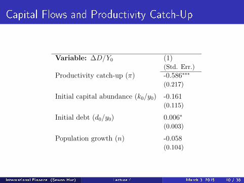
Variable: ∆D/Y0 (1) (2) (3)(Std. Err.) (Std. Err.) (Std. Err.)
Productivity catch-up (π) -0.586∗∗∗ -0.456∗∗ -0.697∗∗∗
(0.217) (0.209) (0.227)
Initial capital abundance (k0/y0) -0.161 -0.126 -0.081(0.115) (0.109) (0.107)
Initial debt (d0/y0) 0.006∗ 0.004 0.001(0.003) (0.003) (0.003)
Population growth (n) -0.058 -0.098 -0.073(0.104) (0.099) (0.096)
Openness (Chinn-Ito) -0.141∗∗ -0.115∗
(0.063) (0.062)
Openness x π -0.455∗
(0.197)
Intercept 0.516 0.576 0.536(0.315) (0.299) (0.289)
Number of observations 68 67 67Adjusted-R2 0.174 0.157 0.214
Table 2: Estimation results : Regression of observed capital inflows ∆D/Y0 on initial condi-tions (capital abundance, external debt), population growth, productivity catch-up (π) andthe Chinn and Ito (2008) index of capital account openness.
International Finance (Sewon Hur) Lecture 4 March 3, 2015 10 / 38

Wedge Analysis
Business Cycle Accounting (Chari, Kehoe, and Macgrattan
2007): large class of DSGE models are observationally equivalent
to a benchmark RBC model with �wedges� in the FOCs.
Capital wedge: tax τk on gross return to capital Rt (e.g. taxes,
credit market imperfections, bureaucracy, bribery/corruption)
Savings wedge: tax τs on capital income (e.g. domestic �nancial
repression)
Ct + Kt+1 = (1− τs)(Rt(1− τk)Kt − R∗Dt) + Dt+1 + wt + Tt
where Tt = τkRtKt + τsR∗(Kt − Dt) lump-sum transfer
Euler equation1
ct= βR∗(1− τs)
1
ct+1
International Finance (Sewon Hur) Lecture 4 March 3, 2015 11 / 38

Capital Wedge
Capital and savings wedges can be calculated to match
investment and savings rates
Capital wedge lower in high productivity growth economies
(better institutions and lower distortions)
AGO
ARG
BEN
BGDBOL
BRA
BWA
CHLCHN
CIV CMR
COG
COL
CRI
CYP
DOM
ECU
EGY
ETH
FJI
GAB
GHAGTM
HKG
HND
HTI
IDN
IND
IRNISRJAM
JOR
KEN
KOR
LKA
MAR
MDG
MEX
MLI
MOZ
MUSMWI
MYS
NERNGA
NPL
PAK
PANPER
PHL
PNG
PRY
RWA
SEN
SGP
SLV
SYR
TGO
THA
TTOTUN
TURTWN
TZA
UGA
URY
VEN
ZAF
01
02
03
04
05
0
Capital W
edge (
%)
−.75 −.5 −.25 0 .25 .5 .75 1
Productivity Catch−Up
Figure 3: Productivity catch-up (π) and capital wedge (τ k).
AGO ARG
BEN
BGD
BOL
BRA
BWA
CHL
CHN
CIV
CMR
COG
COL
CRI
CYP
DOM
ECU
EGY
ETH
FJIGABGHA
GTM
HKG
HND
HTIIDN
IND
IRN
ISR
JAM
JOR
KEN
LKA
MAR
MEX
MLI
MOZ
MUS
MWI
MYS
NER
NGA
NPL
PAK
PAN
PER
PHLPNGPRY
RWA
SEN
SGP
SLV
SYR
TGO
THA
TTO
TUN
TUR
TWN
TZA
UGA
URY
VEN
ZAF
KOR
MDG
−2
0−
10
01
02
0
Pre
dic
ted C
hange in E
xte
rnal D
ebt (r
ela
tive to initia
l outp
ut)
−.75 −.5 −.25 0 .25 .5 .75 1
Productivity Catch−Up
Figure 4: Productivity catch-up (π) and capital inflows(
∆DY0
)predicted by the model with
capital wedges.
18
International Finance (Sewon Hur) Lecture 4 March 3, 2015 12 / 38

Capital Wedge
This worsens the allocation puzzle
Plot of productivity catch-up and capital in�ows predicted by the
model with capital wedges
AGO
ARG
BEN
BGDBOL
BRA
BWA
CHLCHN
CIV CMR
COG
COL
CRI
CYP
DOM
ECU
EGY
ETH
FJI
GAB
GHAGTM
HKG
HND
HTI
IDN
IND
IRNISRJAM
JOR
KEN
KOR
LKA
MAR
MDG
MEX
MLI
MOZ
MUSMWI
MYS
NERNGA
NPL
PAK
PANPER
PHL
PNG
PRY
RWA
SEN
SGP
SLV
SYR
TGO
THA
TTOTUN
TURTWN
TZA
UGA
URY
VEN
ZAF
01
02
03
04
05
0
Capital W
edge (
%)
−.75 −.5 −.25 0 .25 .5 .75 1
Productivity Catch−Up
Figure 3: Productivity catch-up (π) and capital wedge (τ k).
AGO ARG
BEN
BGD
BOL
BRA
BWA
CHL
CHN
CIV
CMR
COG
COL
CRI
CYP
DOM
ECU
EGY
ETH
FJIGABGHA
GTM
HKG
HND
HTIIDN
IND
IRN
ISR
JAM
JOR
KEN
LKA
MAR
MEX
MLI
MOZ
MUS
MWI
MYS
NER
NGA
NPL
PAK
PAN
PER
PHLPNGPRY
RWA
SEN
SGP
SLV
SYR
TGO
THA
TTO
TUN
TUR
TWN
TZA
UGA
URY
VEN
ZAF
KOR
MDG
−2
0−
10
01
02
0
Pre
dic
ted C
hange in E
xte
rnal D
ebt (r
ela
tive to initia
l outp
ut)
−.75 −.5 −.25 0 .25 .5 .75 1
Productivity Catch−Up
Figure 4: Productivity catch-up (π) and capital inflows(
∆DY0
)predicted by the model with
capital wedges.
18
International Finance (Sewon Hur) Lecture 4 March 3, 2015 13 / 38

Private Returns Equalization
Naive private returns Rn ≡ αY /K − δWedge-adjusted returns (1− τk)(1 + Rn)− 1
AGO
ARG
BEN
BGDBOL
BRA
BWA
CHLCHN
CIV
CMRCOG COL
CRICYP
DOM
ECU
EGY
ETH
FJIGAB
GHAGTM
HKGHND
HTI
IDN
IND
IRNISRJAM
JOR
KEN
KOR
LKAMAR
MDG
MEX
MLI
MOZ
MUS
MWI
MYS
NER
NGANPL
PAK
PANPERPHL
PNGPRY
RWA
SEN
SGP
SLVSYR
TGO
THA
TTOTUNTUR TWN
TZA
UGA
URYVEN
ZAF
020
40
60
80
100
120
Naiv
e M
PK
(perc
ent)
0 10000 20000 30000
Real GDP per capita (2000)
AGO ARGBENBGDBOL BRABWACHLCHNCIV
CMR
COG
COLCRI CYPDOMECUEGY
ETH FJI GABGHAGTM HKGHND
HTI
IDNIND
IRNISRJAM
JORKEN KORLKAMAR
MDGMEX
MLIMOZ MUS
MWI
MYS
NER
NGA
NPLPAK PANPERPHLPNGPRYRWA
SEN SGPSLVSYR
TGOTHA
TTOTUNTUR TWN
TZA
UGA
URYVENZAF0
20
40
60
80
100
120
Wedge−
Adju
ste
d M
PK
(perc
ent)
0 10000 20000 30000
Real GDP per capita (2000)
Figure 5: Naıve and Wedge-adjusted Marginal Product of Capital in year 2000.
As a final comment, it is interesting to note that the capital wedge plays a similar roleas adjusting for non-reproducible capital and relative price effects discussed in Caselli andFeyrer (2007). Those authors argue that, while naıve estimates of the marginal productof capital vary enormously across countries, the returns to capital are essentially the sameonce the estimates are adjusted for cross-country differences in the share of non-reproduciblecapital in total capital and in the price of reproducible capital in terms of output, whichare both higher in less advanced countries. Our approach leads to the same cross-countrycompression in the estimates of the returns on capital, but this is achieved by the capitalwedge τ k.
To illustrate this point, Figure 5 compares the naive estimate of private returns (leftpanel), defined as RN = αY/K − δ, and the wedge-adjusted return (right panel), RW =(1− τ k) (1 +RN) − 1, against 2000 income per capita. The left panel indicates enormousvariation in the naıve estimate, between 3.6 percent (Singapore) and 110 percent (Haiti),with a mean of 22.3 percent. By contrast, the wedge-adjusted return varies between -2.5percent (Nigeria) and 43 percent (Haiti, a clear outlier), with a mean of 6.3 percent. Theamount of compression is remarkable, given that the capital wedge is not calibrated to ensureprivate returns equalization. Our results thus parallel those of Caselli and Feyrer (2007):private returns to capital appear remarkably similar across countries.34
To summarize, introducing investment wedges to match observed investment rates intothe model does not help to solve the allocation puzzle, but is consistent with the equalizationof private returns to capital across countries. We now turn to the saving wedges.
34In Gourinchas and Jeanne (2007) we also look at the correlation between productivity growth and capitalinflows when productivity is measured based on the model with non-reproducible capital of Caselli and Feyrer(2007). We find the same negative correlation.
19
International Finance (Sewon Hur) Lecture 4 March 3, 2015 14 / 38

Savings Wedge
Savings wedge lower in high productivity growth economies
(subsidize vs tax)
AGO
ARG
BEN
BGD
BOL
BRA
BWA
CHL
CHN
CIV
CMR
COG
COL
CRI
CYP
DOM
ECU
EGY
ETH
FJIGABGHA
GTM
HKG
HND
HTIIDN
IND
IRN
ISR
JAMJOR
KEN
LKA
MAR
MEX
MLI
MOZ
MUS
MWI
MYS
NERNGA
NPL
PAK
PAN
PER
PHLPNG
PRY
RWA
SEN
SGP
SLV
SYR
TGO
THA
TTO
TUN
TUR
TWN
TZA
UGA
URY
VEN
ZAF
KOR
MDG
−5
05
Savin
g W
edge (
perc
ent)
−.75 −.5 −.25 0 .25 .5 .75 1
Productivity Catch−Up
Figure 6: Productivity catch-up (π) and saving wedges (τ s).
productivity catch-up and distortions in the accumulation of domestic capital summarizedby the capital wedge τ k. Not surprisingly, the convergence component is positive for Asiaand Latin America (capital scarce regions) and negative for Africa (capital abundant), whilethe investment component is positive for Asia (productivity catch-up) and negative for LatinAmerica and Africa (productivity decline). The sum of these two terms is negatively corre-lated with observed capital inflows.
This illustrates the extent to which the allocation puzzle is a saving puzzle: adjustinginvestment rates to account for physical capital accumulation is not enough to account forpatterns of capital flows across countries. The saving wedge is essential to account forthe observed pattern of net capital flows across developing countries. Our wedge analysisindicates that Asia subsidizes saving (τ s = −1.14 percent) whereas Latin America and Africatax savings similarly (τ s = 1.8 percent). Similarly, the saving tax decreases with levels ofdevelopment.
5 Public vs. private flows
Having established that the allocation puzzle is a saving puzzle, we now offer a different cutof the data. This section documents differences between the behavior of public capital flows(defined as flows that go to or emanates from the public sector) and that of private flows(defined as the residual). We look first at official aid flows, and then at broader measures ofpublic flows.38 One could argue that the basic neoclassical framework may not be appropriate
38Our results on aid flows were reported in previous versions of this paper. The analysis was extended topublic flows as defined by Aguiar and Amador (2011) following a suggestion of the editor and referees.
21
International Finance (Sewon Hur) Lecture 4 March 3, 2015 15 / 38
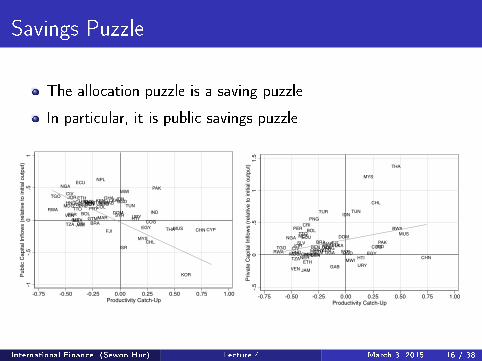
Savings Puzzle
The allocation puzzle is a saving puzzle
In particular, it is public savings puzzle
PHLIND
PAK
KOR
MYS
CHNTHA
IDN
NPL
FJI
PNG BGDTUR LKA
ECU
BOLGTM
COL
HTI
PAN
SLVURYVEN
BRACRI
HND
PERPRY
DOMTTO
CHL
JAM
ARG
MEX
MWI
TUNCMR
SYR
KEN
MUS
NER GAB
TZA
SENRWA
JOR
COG
ISR
BENTGO
CYPEGY
CIVNGA
ETHMDG
UGA
MAR
MLIGHA
-1-.5
0.5
1Pu
blic
Capi
tal I
nflow
s (re
lativ
e to
initia
l out
put)
-0.75 -0.50 -0.25 0.00 0.25 0.50 0.75 1.00Productivity Catch-Up
(a) Net Public Capital Inflows
PNG
FJI PAK
THA
IND
MYS
LKABGD
NPL
PHL
IDN
CHN
TUR
URYVEN
HND
BRACOL
DOM
JAM
ECU
HTI
PER BOL
GTMPAN
MEX
ARGPRY
CHL
SLV
TTO
CRI
BEN MAR
EGYSYR
MWI
COGTGO CIVRWA CMRNERETH
TUN
GHA
SENMDG
NGA
BWA
JORMLI UGA
TZAKEN
GAB
MUS
-.50
.51
1.5
Priva
te C
apita
l Infl
ows
(rela
tive
to in
itial o
utpu
t)
-0.75 -0.50 -0.25 0.00 0.25 0.50 0.75 1.00Productivity Catch-Up
(b) Net Private Capital Inflows
Note: top panel reports ∆Dpub/Y0 against π. Bottom panel reports ∆Dpriv/Y0 against π.
Figure 8: Productivity catch-up (π) and change in public and private external debt.
26
International Finance (Sewon Hur) Lecture 4 March 3, 2015 16 / 38

Savings Puzzle
Why are emerging economies accumulating so much foreign
reserves (savings)?
Recent papers on reserves accumulation
reserves to smooth consumption against exogenous crises: Alfaro
and Kanczuk (2009), Bianchi et al. (2012), Caballero and
Panageas (2007), Jeanne and Ranciere (2011)
NFA prevents crises: Durdu et al (2009), Mendoza (2010)
reserves prevent crises: Hur and Kondo (2013), Kim (2008)
International Finance (Sewon Hur) Lecture 4 March 3, 2015 17 / 38
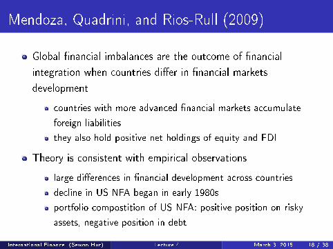
Mendoza, Quadrini, and Rios-Rull (2009)
Global �nancial imbalances are the outcome of �nancial
integration when countries di�er in �nancial markets
development
countries with more advanced �nancial markets accumulate
foreign liabilities
they also hold positive net holdings of equity and FDI
Theory is consistent with empirical observations
large di�erences in �nancial development across countries
decline in US NFA began in early 1980s
portfolio compostition of US NFA: positive position on risky
assets, negative position in debt
International Finance (Sewon Hur) Lecture 4 March 3, 2015 18 / 38
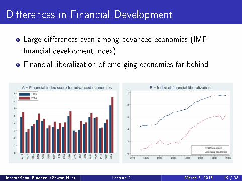
Di�erences in Financial Development
Large di�erences even among advanced economies (IMF
�nancial development index)
Financial liberalization of emerging economies far behind
0
.1
.2
.3
.4
.5
.6
.7
.8
AU
S
AU
T
BE
L
CA
N
DE
N
DE
U
ES
P
FIN
FR
A
GB
R
GR
C
ITA
JPN
NLD
NO
R
PR
T
SW
E
US
A
A − Financial index score for advanced economies
1995
2004
0
.2
.4
.6
.8
1
1970 1975 1980 1985 1990 1995 2000 2005
OECD countries
Emerging economies
B − Index of financial liberalization
Figure 1: Indices of financial markets heterogeneity. The index in panel Ais from IMF (2006). The index in panel B is from Abiad, Detragiache andTressel (2007). See appendix A for the definition of variables.
3
0
.1
.2
.3
.4
.5
.6
.7
.8
AU
S
AU
T
BE
L
CA
N
DE
N
DE
U
ES
P
FIN
FR
A
GB
R
GR
C
ITA
JPN
NLD
NO
R
PR
T
SW
E
US
A
A − Financial index score for advanced economies
1995
2004
0
.2
.4
.6
.8
1
1970 1975 1980 1985 1990 1995 2000 2005
OECD countries
Emerging economies
B − Index of financial liberalization
Figure 1: Indices of financial markets heterogeneity. The index in panel Ais from IMF (2006). The index in panel B is from Abiad, Detragiache andTressel (2007). See appendix A for the definition of variables.
3
International Finance (Sewon Hur) Lecture 4 March 3, 2015 19 / 38

Composition of NFA
US increased risky assets and reduced riskless assets (net)
Emerging economies reduced risky assets and increased riskless
assets (net)
−10
−8
−6
−4
−2
0
2
4
Per
cent
of w
orld
GD
P
1970 1975 1980 1985 1990 1995 2000 2005
United States
OECD countries except US
Emerging economies
A − NFA in debt and international reserves
−10
−8
−6
−4
−2
0
2
4
Per
cent
of w
orld
GD
P
1970 1975 1980 1985 1990 1995 2000 2005
United States
OECD countries except US
Emerging economies
B − NFA in portfolio equity and FDI
Figure 3: Net foreign asset positions in debt instruments and risky assets.The graphs are constructed using data from Lane and Milesi-Ferretti (2006).See appendix A.
5
−10
−8
−6
−4
−2
0
2
4
Per
cent
of w
orld
GD
P
1970 1975 1980 1985 1990 1995 2000 2005
United States
OECD countries except US
Emerging economies
A − NFA in debt and international reserves
−10
−8
−6
−4
−2
0
2
4
Per
cent
of w
orld
GD
P
1970 1975 1980 1985 1990 1995 2000 2005
United States
OECD countries except US
Emerging economies
B − NFA in portfolio equity and FDI
Figure 3: Net foreign asset positions in debt instruments and risky assets.The graphs are constructed using data from Lane and Milesi-Ferretti (2006).See appendix A.
5
International Finance (Sewon Hur) Lecture 4 March 3, 2015 20 / 38

Model
Multi-country DSGE model with incomplete markets
Idiosyncratic shocks to endowment and investment
Two frictions: limited enforcement and limited liability
International Finance (Sewon Hur) Lecture 4 March 3, 2015 21 / 38

Simple Model
Two countries, i = 1, 2, each populated by continuum of agents
Each country endowed with unit supply of non-reproducible,
international immobile asset, traded at price P it
This asset can be used to produce yt+1 = zt+1kνt where zt+1 is
an idiosyncratic investment shock. Agents can invest
domestically or abroad, but not diversify (relaxed later)
Agents receive an idiosyncratic stochastic endowment wt , which
follows a Markov process
Maximize∑∞
t=0 βtU(ct)
No aggregate uncertainty
International Finance (Sewon Hur) Lecture 4 March 3, 2015 22 / 38
Simple Model
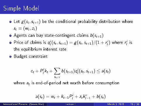
Let g(st , st+1) be the conditional probability distribution where
st ≡ (wt , zt)
Agents can buy state-contingent claims b(st+1)
Price of claims is qit(st , st+1) = g(st , st+1)/(1 + r it ) where r it is
the equilibrium interest rate
Budget constraint
ct + P itkt +
∑
st+1
b(st+1)qit(st , st+1) ≤ a(st)
where at is end-of-period net worth before consumption
a(st) = wt + kt−1Pit + ztk
νt−1 + b(st)
International Finance (Sewon Hur) Lecture 4 March 3, 2015 23 / 38

Financial Frictions
If markets were complete, agents would perfectly insure against
endowment and investment risks
Agents can divert 1− φi of income; φi represents degree of
enforcement
Two frictions: limited enforcement and limited liability
a(sj)− a(s1) ≥ (1− φi) [wj − w1 + (zj − z1)kνt ]
a(sj) ≥ 0
where s1 denotes the worst possible realization
φi = 1 implies constant consumption and φi = 0 implies no
insurance
International Finance (Sewon Hur) Lecture 4 March 3, 2015 24 / 38
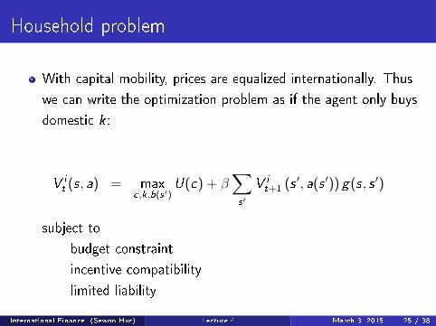
Household problem
With capital mobility, prices are equalized internationally. Thus
we can write the optimization problem as if the agent only buys
domestic k :
V it (s, a) = max
c,k,b(s′)U(c) + β
∑
s′
V it+1 (s ′, a(s ′)) g(s, s ′)
subject to
budget constraint
incentive compatibility
limited liability
International Finance (Sewon Hur) Lecture 4 March 3, 2015 25 / 38

Autarky Equilibrium
Given �nancial development φi and initial distributions M it(s, k , b) for
i = 1, 2, an autarky equilibrium is policy functions, value functions,
prices, and distributions such that
1 policy functions and value functions solve household problem
2 asset markets clear :´s,k,b
k itM
it(s, k , b) = 1,´
s,k,b,s′bit(s, a, s
′)M it(s, k , b)g(s, s ′) = 0 for i = 1, 2
3 distributions are consistent with initial distributions, individual
policies, and stochastic processes for idiosyncratic shocks
International Finance (Sewon Hur) Lecture 4 March 3, 2015 26 / 38

Integrated Equilibrium
The de�nition of integrated equilibrium is identical except additional
conditions on prices (q1t = q2
t , P1t = P2
t ) and market clearing
conditions:
∑
i=1,2
ˆs,k,b
k itM
it(s, k , b) = 2
∑
i=1,2
ˆs,k,b,s′
bit(s, a, s′)M i
t(s, k , b)g(s, s ′) = 0
International Finance (Sewon Hur) Lecture 4 March 3, 2015 27 / 38

Net foreign asset position
NFA of country i is given by
NFAit =
ˆs,k,b
bit(s, a, s′)M i
t(s, k , b)g(s, s ′)+
ˆs,k,b
[k it − 1
]PtM
it(s, k , b)
International Finance (Sewon Hur) Lecture 4 March 3, 2015 28 / 38

Characterization
First consider the case with endowment shocks only.
Financial autarky regime and φ = φ (such that IC not binding).
Then r = 1/β − 1 since agents can perfectly insure against
idiosyncratic risk, and there are no precautionary savings. Also
Rt+1 = 1 + rt
Financial autarky regime and φ = 0 (no state-contingent
claims). Then r < 1/β − 1 since agents cannot perfectly insure
against idiosyncratic risk, and there are precautionary savings
(since U ′ is convex). Also Rt+1 = 1 + rt
All agents invest k = 1 since marginal return on productive asset
is equal to the interest rate
International Finance (Sewon Hur) Lecture 4 March 3, 2015 29 / 38
Proposition 1
Suppose that φ1 = φ and φ2 = 0. In the integrated equilibrium,
rt < 1/β − 1 and country 1 accumulates a negative NFA but
holds a zero net position in the productive asset
r aut1 > rint > r aut2
Demand for assets fall in country 1 and rise in country 2, hence
the country with deeper �nancial markets ends up with a
negative NFA
International Finance (Sewon Hur) Lecture 4 March 3, 2015 30 / 38

Characterization
Now consider the case with investment shocks only.
Financial autarky regime and φ = φ (such that IC not binding).
Then r = 1/β − 1 since agents can perfectly insure against
idiosyncratic risk. Now ERt+1 = 1 + rt , but still all agents invest
k = 1
Financial autarky regime and φ = 0 (no state-contingent
claims). Then r < 1/β − 1 since agents cannot perfectly insure
against idiosyncratic risk (precautionary savings). But now there
is a marginal risk premium for the risky asset
ERt+1 − (1 + rt) = −Cov(Rt+1,U′(c(z ′))
EU ′(c(z ′))> 0
International Finance (Sewon Hur) Lecture 4 March 3, 2015 31 / 38

Proposition 2
Suppose that φ1 = φ and φ2 = 0. In the integrated equilibrium,
rt < 1/β − 1. Country 1 has a negative NFA but a positive
position on the productive asset. Moreover, the average return of
country 1's foreign assets is larger than the cost of its liabilities.
The same proposition holds for the case with both endowment
and investment shocks.
International Finance (Sewon Hur) Lecture 4 March 3, 2015 32 / 38

General Model
Extend the simple model
N countries
diversi�able managerial capital yt+1 =∑N
i=1 zi ,t+1A1−νit kνit with∑N
i=1 Ait = 1
second source of �nancial heterogeneity (a(sj) ≥ ai limited
liability) in addition to φ
di�erences in economic size of countries
International Finance (Sewon Hur) Lecture 4 March 3, 2015 33 / 38

US vs ROW
µ1 = 0.3 to match US share of world GDP, 30 percent
φ1 = 0.3, φ2 = 0 (contingent claims partly available in US)
International Finance (Sewon Hur) Lecture 4 March 3, 2015 34 / 38
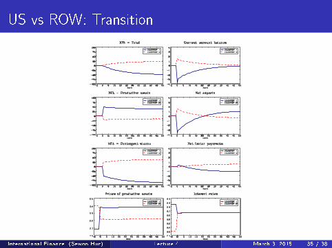
US vs ROW: Transition
Figure 6: Transition dynamics after capital markets liberalization.
28
International Finance (Sewon Hur) Lecture 4 March 3, 2015 35 / 38
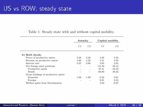
US vs ROW: steady state
Table 1: Steady state with and without capital mobility.
Autarky Capital mobility
C1 C2 C1 C2
A) Both shocksPrices of productive assets 3.08 3.40 3.38 3.22Returns on productive assets 4.80 4.30 4.41 4.58Interest rate 3.25 2.60 3.05 3.05Net foreign asset positions - - -51.39 22.12Productive assets - - 37.41 -16.10Bonds - - -88.80 38.22
Gross holdings of productive assetsDomestic 1.00 1.00 0.24 0.61Foreign - - 0.91 0.33
Welfare gains from liberalization 2.63 -0.27
B) Endowment shocks onlyPrices of productive assets 2.95 3.22 3.14 3.14Returns on productive assets 5.08 4.66 4.78 4.78Interest rate 3.81 3.49 3.58 3.58Net foreign asset positions - - -38.69 16.58Productive assets - - 0.00 0.00Bonds - - -38.69 16.58
Gross holdings of productive assetsDomestic 1.00 1.00 1.00 1.00Foreign - - 0.00 0.00
Welfare gains from liberalization 1.66 -0.77
C) Investment shocks onlyPrices of productive assets 1.41 1.37 1.45 1.38Returns on productive assets 10.63 10.90 10.41 10.83Interest rate 7.35 6.58 7.33 7.33Net foreign asset positions - - -5.38 2.31Productive assets - - 14.08 -6.04Bonds - - -19.46 8.35
Gross holdings of productive assetsDomestic 1.00 1.00 0.23 0.61Foreign - - 0.91 0.33
Welfare gains from liberalization 0.60 0.20
Notes: Foreign asset positions are in percentage of domestic income (endowment plusdomestic investment income). Gross positions of productive assets are units of k per-capita. Welfare gains are in percentage of consumption.
26
International Finance (Sewon Hur) Lecture 4 March 3, 2015 36 / 38

US vs ROW: welfare
Two sources of welfare gains/losses
diversi�cation of investment risk
cost of borrowing/lending
In country 1, all agents gain from liberalization, and the gains
are especially high for low wealth agents
In country 2, agents also gain from diversi�cation of risk, but
the increase in interest rates relative to autarky hurt the poor.
Overall, they su�er a welfare loss.
International Finance (Sewon Hur) Lecture 4 March 3, 2015 37 / 38
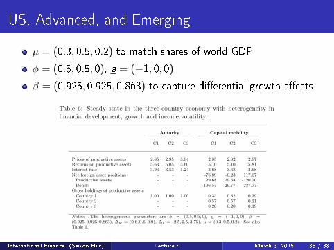
US, Advanced, and Emerging
µ = (0.3, 0.5, 0.2) to match shares of world GDP
φ = (0.5, 0.5, 0), a = (−1, 0, 0)
β = (0.925, 0.925, 0.863) to capture di�erential growth e�ects
with greater uncertainty at the individual level.14 Therefore, if we want tocapture the differences between industrialized and emerging economies thatare relevant for savings, we should allow for three sources of heterogeneity:financial markets development, economic growth and income volatility.
We add heterogeneity in growth and income volatility to the three-countrymodel examined above. An easy way to capture differences in growth ratesis to assume that countries have different discount rates. If β is the discountfactor for industrialized countries and the growth rate differential betweenemerging and industrialized countries is 1 + g, then the discount factor ofemerging countries is β = β/(1 + g)σ. Assuming an annual growth differ-ential of 3.5 percent, and given the baseline parametrization β = 0.925 andσ = 2, the discount factor for C3 is β = 0.925/1.0352 = 0.863. Under theseassumptions, if C1 and C2 grow at about 2 percent per year, emerging coun-tries (C3) grow at 5.5 percent per year. To account for the higher uncertaintyfaced by agents in emerging economies, we assume that the standard devia-tions of endowment and investment shocks in C3 are 50 percent higher thanin C1 and C2.
Table 6: Steady state in the three-country economy with heterogeneity infinancial development, growth and income volatility.
Autarky Capital mobility
C1 C2 C3 C1 C2 C3
Prices of productive assets 2.65 2.95 3.84 2.85 2.82 2.87Returns on productive assets 5.63 5.05 3.60 5.10 5.10 5.81Interest rate 3.96 3.53 1.24 3.68 3.68 3.68Net foreign asset positions - - - -76.89 -0.23 117.07Productive assets - - - 29.68 29.54 -120.70Bonds - - - -106.57 -29.77 237.77
Gross holdings of productive assetsCountry 1 1.00 1.00 1.00 0.33 0.32 0.19Country 2 - - - 0.57 0.57 0.21Country 3 - - - 0.20 0.20 0.19
Notes: The heterogeneous parameters are φ = (0.5, 0.5, 0), a = (−1, 0, 0), β =(0.925, 0.925, 0.863), ∆w = (0.6, 0.6, 0.9), ∆z = (2.5, 2.5, 3.75), µ = (0.3, 0.5, 0.2). See alsoTable 1.
14An indicator of this is that inequality tends to increase during phases of rapid growth.See Khan & Riskin (2001) and Naughton (2007). Also, several emerging economies haveexperienced Sudden Stops after entering the global financial markets.
39
International Finance (Sewon Hur) Lecture 4 March 3, 2015 38 / 38


![fJi)uEZíg j s5 - OAK Centralcentral.oak.go.kr/repository/journal/13228/BBROBV_2014_v...^ t½{ v \ fJi)uEZíg j s5 \ fJu)fI Iv Eh]{ v \ fJi)uEz¡Z±uîue Zíg j s5u1gµf E\ tñ a`Ñu9ZéZu-sÝ[Yj](https://img.dokumen.tips/doc/110x75/5b1bc6487f8b9a1e258f280a/fjiuezig-j-s5-oak-t-v-fjiuezig-j-s5-fjufi-iv-eh-v-fjiuezzuiue.jpg)