www.olympus-ims.com

Ultrasonic TransducersTechnical Notes

Basic Ultrasonic Principles . . . . . . . . . . . . . . . . . . . . . . . . . . . . . . . . . . . . . . . . . . . . 41-42. a ..What.is.Ultrasound. b ..Frequency,.Period.and.Wavelength. c ..Velocity.of.Ultrasound.and.Wavelength. d ..Wave.Propagation.and.Particle.Motion. e ..Applying.Ultrasound. f ..Sensitivity.and.Resolution

Advanced Definitions and Formulas . . . . . . . . . . . . . . . . . . . . . . . . . . . . . . . . . . . . 42-44. a ..Transducer.Waveform.and.Spectrum. b ..Acoustic.Impedance,.Reflectivity,.and.Attenuation. c ..Sound.Field. d ..Other.Parameters.of.a.Sound.Beam

Design Characteristics of Transducers . . . . . . . . . . . . . . . . . . . . . . . . . . . . . . . . . . . . . . 44. a ..What.is.an.Ultrasonic.Transducer?. b ..The.Active.Element. c ..Backing. d ..Wear.Plate

Transducer Specific Principles . . . . . . . . . . . . . . . . . . . . . . . . . . . . . . . . . . . . . . . . . 44-47. a ..Dual.Element.Transducers. b ..Angle.Beam.Transducers. c ..Delay.Line.Transducers. d ..Immersion.Transducers. e ..Normal.Incidence.Shear.Wave.Transducers

Transducer Excitation Guidelines . . . . . . . . . . . . . . . . . . . . . . . . . . . . . . . . . . . . . . . . . . 47

Cables . . . . . . . . . . . . . . . . . . . . . . . . . . . . . . . . . . . . . . . . . . . . . . . . . . . . . . . . . . . . . 47-48

Near Field Distance of Flat Transducers in Water . . . . . . . . . . . . . . . . . . . . . . . . . . . . . 48

Acoustic Properties of Materials . . . . . . . . . . . . . . . . . . . . . . . . . . . . . . . . . . . . . . . . . . . 49

40

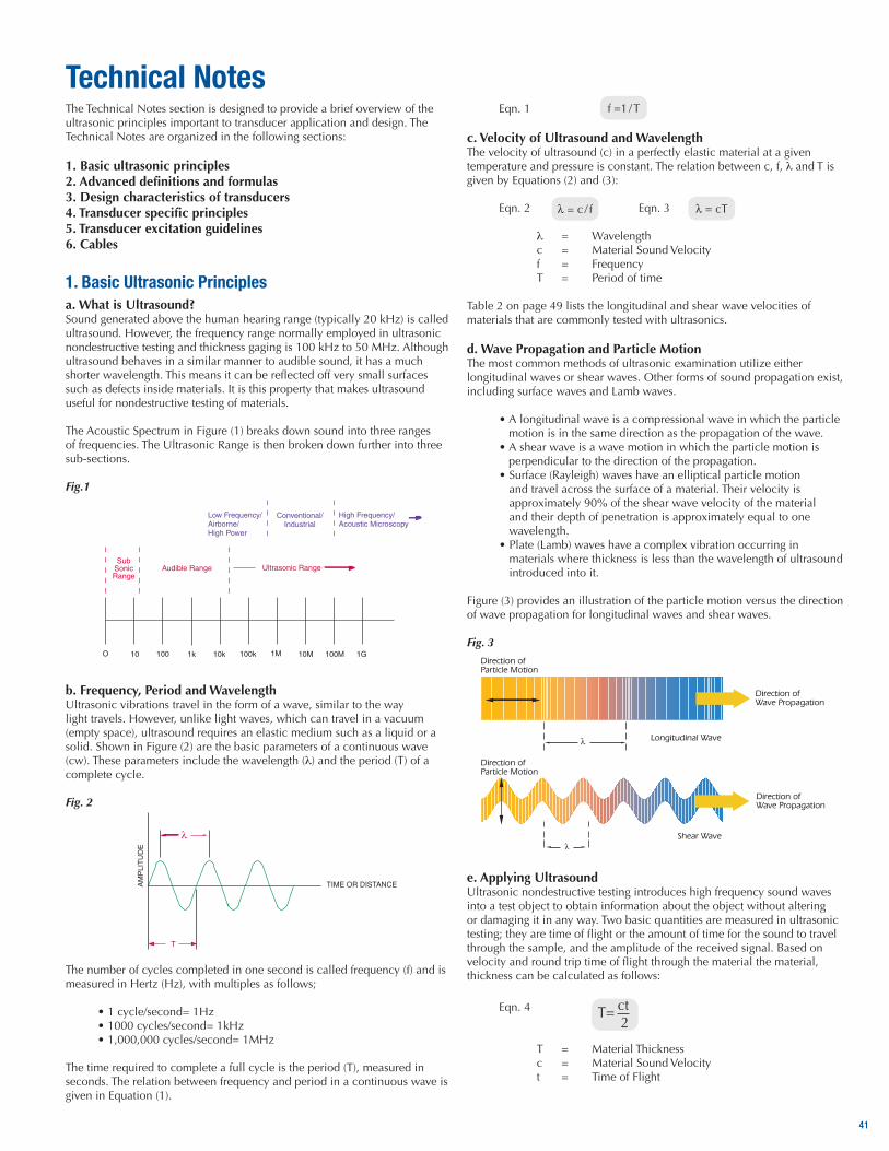
The Technical Notes section is designed to provide a brief overview of the ultrasonic principles important to transducer application and design. The Technical Notes are organized in the following sections:

1. Basic ultrasonic principles2. Advanced definitions and formulas3. Design characteristics of transducers4. Transducer specific principles5. Transducer excitation guidelines6. Cables

1. Basic Ultrasonic Principlesa. What is Ultrasound? Sound generated above the human hearing range (typically 20 kHz) is called ultrasound. However, the frequency range normally employed in ultrasonic nondestructive testing and thickness gaging is 100 kHz to 50 MHz. Although ultrasound behaves in a similar manner to audible sound, it has a much shorter wavelength. This means it can be reflected off very small surfaces such as defects inside materials. It is this property that makes ultrasound useful for nondestructive testing of materials.

The Acoustic Spectrum in Figure (1) breaks down sound into three ranges of frequencies. The Ultrasonic Range is then broken down further into three sub-sections.

Fig.1

b. Frequency, Period and WavelengthUltrasonic vibrations travel in the form of a wave, similar to the way light travels. However, unlike light waves, which can travel in a vacuum (empty space), ultrasound requires an elastic medium such as a liquid or a solid. Shown in Figure (2) are the basic parameters of a continuous wave (cw). These parameters include the wavelength (l) and the period (T) of a complete cycle.

Fig. 2

The number of cycles completed in one second is called frequency (f) and is measured in Hertz (Hz), with multiples as follows;

• 1 cycle/second= 1Hz • 1000 cycles/second= 1kHz • 1,000,000 cycles/second= 1MHz

The time required to complete a full cycle is the period (T), measured in seconds. The relation between frequency and period in a continuous wave is given in Equation (1).

Eqn. 1

c. Velocity of Ultrasound and WavelengthThe velocity of ultrasound (c) in a perfectly elastic material at a given temperature and pressure is constant. The relation between c, f, l and T is given by Equations (2) and (3):

Eqn. 2 Eqn. 3

l = Wavelengthc = Material Sound Velocityf = FrequencyT = Period of time

Table 2 on page 49 lists the longitudinal and shear wave velocities of materials that are commonly tested with ultrasonics.

d. Wave Propagation and Particle MotionThe most common methods of ultrasonic examination utilize either longitudinal waves or shear waves. Other forms of sound propagation exist, including surface waves and Lamb waves.

• A longitudinal wave is a compressional wave in which the particle motion is in the same direction as the propagation of the wave.

• A shear wave is a wave motion in which the particle motion is perpendicular to the direction of the propagation.

• Surface (Rayleigh) waves have an elliptical particle motion and travel across the surface of a material. Their velocity is approximately 90% of the shear wave velocity of the material and their depth of penetration is approximately equal to one wavelength.

• Plate (Lamb) waves have a complex vibration occurring in materials where thickness is less than the wavelength of ultrasound introduced into it.

Figure (3) provides an illustration of the particle motion versus the direction of wave propagation for longitudinal waves and shear waves.

Fig. 3

e. Applying UltrasoundUltrasonic nondestructive testing introduces high frequency sound waves into a test object to obtain information about the object without altering or damaging it in any way. Two basic quantities are measured in ultrasonic testing; they are time of flight or the amount of time for the sound to travel through the sample, and the amplitude of the received signal. Based on velocity and round trip time of flight through the material the material, thickness can be calculated as follows:

Eqn. 4

T = Material Thicknessc = Material Sound Velocityt = Time of Flight

Technical Notes

T

Longitudinal Wave

Shear Wave

Direction ofWave Propagation

Direction ofWave Propagation

Direction ofParticle Motion

Direction ofParticle Motion

41

www.olympus-ims.com

Measurements of the relative change in signal amplitude can be used in sizing flaws or measuring the attenuation of a material. The relative change in signal amplitude is commonly measured in decibels. Decibel values are the logarithmic value of the ratio of two signal amplitudes. This can be calculated using the following equation. Some useful relationships are also displayed in the table below;

Eqn. 5

dB = Decibels

A1 = Amplitude of signal 1

A2 = Amplitude of signal 2

f. Sensitivity and Resolution

• Sensitivity is the ability of an ultrasonic system to detect reflectors (or defects) at a given depth in a test material. The greater the signal that is received from a given reflector, the more sensitive the transducer system.

• Axial resolution is the ability of an ultrasonic system to produce simultaneous and distinct indications from reflectors Iocated at nearly the same position with respect to the sound beam.

• Near surface resolution is the ability of the ultrasonic system to detect reflectors located close to the surface of the test piece.

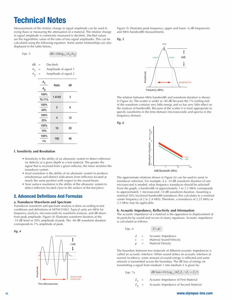
2. Advanced Definitions And Formulasa. Transducer Waveform and Spectrum Transducer waveform and spectrum analysis is done according to test conditions and definitions of ASTM E1065. Typical units are MHz for frequency analysis, microseconds for waveform analysis, and dB down from peak amplitude. Figure (4) illustrates waveform duration at the -14 dB level or 20% amplitude of peak. The -40 dB waveform duration corresponds to 1% amplitude of peak.

Fig. 4

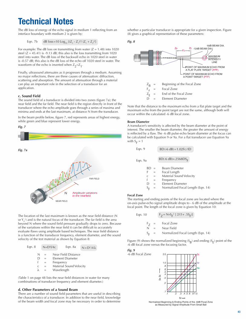
Figure (5) illustrates peak frequency, upper and lower -6 dB frequencies and MHz bandwidth measurements.

Fig. 5

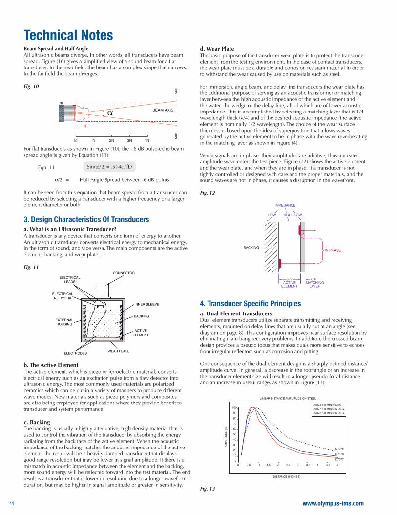
The relation between MHz bandwidth and waveform duration is shown in Figure (6). The scatter is wider at -40 dB because the 1% trailing end of the waveform contains very little energy and so has very little effect on the analysis of bandwidth. Because of the scatter it is most appropriate to specify waveforms in the time domain (microseconds) and spectra in the frequency domain.

Fig. 6

The approximate relations shown in Figure (6) can be used to assist in transducer selection. For example, if a -14 dB waveform duration of one microsecond is needed, what frequency transducer should be selected? From the graph, a bandwidth of approximately 1 to 1.2 MHz corresponds to approximately 1 microsecond -14 dB waveform duration. Assuming a nominal 50% fractional bandwidth transducer, this calculates to a nominal center frequency of 2 to 2.4 MHz. Therefore, a transducer of 2.25 MHz or 3.5 MHz may be applicable.

b. Acoustic Impedance, Reflectivity and AttenuationThe acoustic impedance of a material is the opposition to displacement of its particles by sound and occurs in many equations. Acoustic impedance is calculated as follows:

Eqn. 6

Z = Acoustic Impedancec = Material Sound Velocityr = Material Density

The boundary between two materials of different acoustic impedances is called an acoustic interface. When sound strikes an acoustic interface at normal incidence, some amount of sound energy is reflected and some amount is transmitted across the boundary. The dB loss of energy on transmitting a signal from medium 1 into medium 2 is given by:

Eqn. 7a

Z1 = Acoustic Impedance of First Material

Z2 = Acoustic Impedance of Second Material

Technical Notes

-14dB

Am

plit

ude

Time (Microseconds)

WAVEFORMDURATION

-6dB

Am

plit

ude

Frequency (MHz)

BANDWIDTH

PEAK

LOWER UPPER

Wavefo

rm D

ura

tion

-6dB Bandwidth (MHz)

-40dB-14dB

(Mic

roseconds)

.01

.11

10

10

0

.1 1 10 100

A1Ratio dB

A2

100%1.4142 3

70.71%

100%2 6

50%

100%4 12

25%

100%10 20

10%

100%100 40

1%

42

The dB loss of energy of the echo signal in medium 1 reflecting from an interface boundary with medium 2 is given by:

Eqn. 7b

For example: The dB loss on transmitting from water (Z = 1.48) into 1020 steel (Z = 45.41) is -9.13 dB; this also is the loss transmitting from 1020 steel into water. The dB loss of the backwall echo in 1020 steel in water is -0.57 dB; this also is the dB loss of the echo off 1020 steel in water. The waveform of the echo is inverted when Z2<Z1.

Finally, ultrasound attenuates as it progresses through a medium. Assuming no major reflections, there are three causes of attenuation: diffraction, scattering and absorption. The amount of attenuation through a material can play an important role in the selection of a transducer for an application.

c. Sound FieldThe sound field of a transducer is divided into two zones (figure 7a); the near field and the far field. The near field is the region directly in front of the transducer where the echo amplitude goes through a series of maxima and minima and ends at the last maximum, at distance N from the transducer.

In the beam profile below, figure 7, red represents areas of highest energy, while green and blue represent lower energy.

Fig. 7

Fig. 7a

The location of the last maximum is known as the near field distance (N or Y0

+) and is the natural focus of the transducer. The far field is the area beyond N where the sound field pressure gradually drops to zero. Because of the variations within the near field it can be difficult to accurately evaluate flaws using amplitude based techniques. The near field distance is a function of the transducer frequency, element diameter, and the sound velocity of the test material as shown by Equation 8:

Eqn. 8 Eqn. 8a

N = Near Field DistanceD = Element Diameterf = Frequencyc = Material Sound Velocityl = Wavelength

(Table 1 on page 48 lists the near field distances in water for many combinations of transducer frequency and element diameter.)

d. Other Parameters of a Sound BeamThere are a number of sound field parameters that are useful in describing the characteristics of a transducer. In addition to the near field, knowledge of the beam width and focal zone may be necessary in order to determine

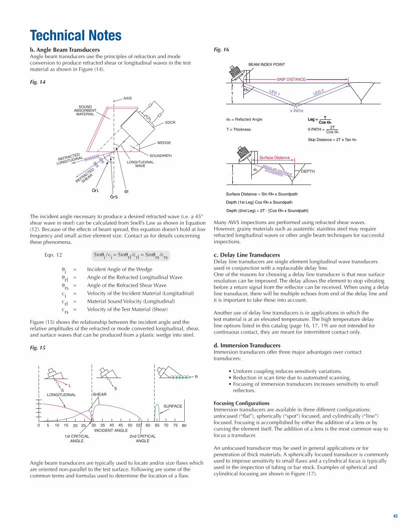
whether a particular transducer is appropriate for a given inspection. Figure (8) gives a graphical representation of these parameters:

Fig. 8

ZB = Beginning of the Focal Zone

Fz = Focal Zone

ZE = End of the Focal Zone

D = Element Diameter

Note that the distance to the maximum echo from a flat plate target and the maximum echo from the point target are not the same, although both will occur within the calculated -6 dB focal zone.

Beam DiameterA transducer’s sensitivity is affected by the beam diameter at the point of interest. The smaller the beam diameter, the greater the amount of energy is reflected by a flaw. The -6 dB pulse-echo beam diameter at the focus can be calculated with Equation 9 or 9a. For a flat transducer use Equation 9a with SF = 1

Eqn. 9

Eqn. 9a

BD = Beam DiameterF = Focal Lengthc = Material Sound Velocity f = FrequencyD = Element DiameterSF = Normalized Focal Length (Eqn. 14)

Focal ZoneThe starting and ending points of the focal zone are located where the on-axis pulse-echo signal amplitude drops to - 6 dB of the amplitude at the focal point. The length of the focal zone is given by Equation 10:

Eqn. 10

FZ = Focal Zone

N = Near Field

SF = Normalized Focal Length (Eqn. 14)

Figure (9) shows the normalized beginning (SB) and ending (SE) point of the -6 dB focal zone versus the focusing factor.

Fig. 9-6 dB Focal Zone

Technical Notes

Amplitude variationsin the nearfield

N

43

www.olympus-ims.com

Beam Spread and Half AngleAll ultrasonic beams diverge. In other words, all transducers have beam spread. Figure (10) gives a simplified view of a sound beam for a flat transducer. In the near field, the beam has a complex shape that narrows. In the far field the beam diverges.

Fig. 10

For flat transducers as shown in Figure (10), the - 6 dB pulse-echo beam spread angle is given by Equation (11):

Eqn. 11

a/2 = Half Angle Spread between -6 dB points

It can be seen from this equation that beam spread from a transducer can be reduced by selecting a transducer with a higher frequency or a larger element diameter or both.

3. Design Characteristics Of Transducersa. What is an Ultrasonic Transducer?A transducer is any device that converts one form of energy to another. An ultrasonic transducer converts electrical energy to mechanical energy, in the form of sound, and vice versa. The main components are the active element, backing, and wear plate.

Fig. 11

b. The Active ElementThe active element, which is piezo or ferroelectric material, converts electrical energy such as an excitation pulse from a flaw detector into ultrasonic energy. The most commonly used materials are polarized ceramics which can be cut in a variety of manners to produce different wave modes. New materials such as piezo polymers and composites are also being employed for applications where they provide benefit to transducer and system performance.

c. BackingThe backing is usually a highly attenuative, high density material that is used to control the vibration of the transducer by absorbing the energy radiating from the back face of the active element. When the acoustic impedance of the backing matches the acoustic impedance of the active element, the result will be a heavily damped transducer that displays good range resolution but may be lower in signal amplitude. If there is a mismatch in acoustic impedance between the element and the backing, more sound energy will be reflected forward into the test material. The end result is a transducer that is lower in resolution due to a longer waveform duration, but may be higher in signal amplitude or greater in sensitivity.

d. Wear PlateThe basic purpose of the transducer wear plate is to protect the transducer element from the testing environment. In the case of contact transducers, the wear plate must be a durable and corrosion resistant material in order to withstand the wear caused by use on materials such as steel.

For immersion, angle beam, and delay line transducers the wear plate has the additional purpose of serving as an acoustic transformer or matching layer between the high acoustic impedance of the active element and the water, the wedge or the delay line, all of which are of lower acoustic impedance. This is accomplished by selecting a matching layer that is 1/4 wavelength thick (l/4) and of the desired acoustic impedance (the active element is nominally 1/2 wavelength). The choice of the wear surface thickness is based upon the idea of superposition that allows waves generated by the active element to be in phase with the wave reverberating in the matching layer as shown in Figure (4).

When signals are in phase, their amplitudes are additive, thus a greater amplitude wave enters the test piece. Figure (12) shows the active element and the wear plate, and when they are in phase. If a transducer is not tightly controlled or designed with care and the proper materials, and the sound waves are not in phase, it causes a disruption in the wavefront.

Fig. 12

4. Transducer Specific Principlesa. Dual Element TransducersDual element transducers utilize separate transmitting and receiving elements, mounted on delay lines that are usually cut at an angle (see diagram on page 8). This configuration improves near surface resolution by eliminating main bang recovery problems. In addition, the crossed beam design provides a pseudo focus that makes duals more sensitive to echoes from irregular reflectors such as corrosion and pitting.

One consequence of the dual element design is a sharply defined distance/amplitude curve. In general, a decrease in the roof angle or an increase in the transducer element size will result in a longer pseudo-focal distance and an increase in useful range, as shown in Figure (13).

Fig. 13

Technical Notes

�

100

90

80

70

60

50

40

30

20

10

00 0.5 1 1.5 2 2.5 3 3.5 4 4.5 5

D7075 5.0 MHz 0 DEG.D7077 5.0 MHz 3.5 DEG.D7078 5.0 MHz 2.6 DEG.

D7075

D7078

D7077

LINEAR DISTANCE AMPLITUDE ON STEEL

DISTANCE (INCHES)

AM

PLI

TU

DE

(%

)

44

b. Angle Beam TransducersAngle beam transducers use the principles of refraction and mode conversion to produce refracted shear or longitudinal waves in the test material as shown in Figure (14).

Fig. 14

The incident angle necessary to produce a desired refracted wave (i.e. a 45° shear wave in steel) can be calculated from Snell’s Law as shown in Equation (12). Because of the effects of beam spread, this equation doesn’t hold at low frequency and small active element size. Contact us for details concerning these phenomena.

Eqn. 12

qi = Incident Angle of the Wedge

qrl = Angle of the Refracted Longitudinal Wave

qrs = Angle of the Refracted Shear Wave

ci = Velocity of the Incident Material (Longitudinal)

crl = Material Sound Velocity (Longitudinal)

crs = Velocity of the Test Material (Shear)

Figure (15) shows the relationship between the incident angle and the relative amplitudes of the refracted or mode converted longitudinal, shear, and surface waves that can be produced from a plastic wedge into steel.

Fig. 15

Angle beam transducers are typically used to locate and/or size flaws which are oriented non-parallel to the test surface. Following are some of the common terms and formulas used to determine the location of a flaw.

Fig. 16

Many AWS inspections are performed using refracted shear waves. However, grainy materials such as austenitic stainless steel may require refracted longitudinal waves or other angle beam techniques for successful inspections.

c. Delay Line TransducersDelay line transducers are single element longitudinal wave transducers used in conjunction with a replaceable delay line.One of the reasons for choosing a delay line transducer is that near surface resolution can be improved. The delay allows the element to stop vibrating before a return signal from the reflector can be received. When using a delay line transducer, there will be multiple echoes from end of the delay line and it is important to take these into account.

Another use of delay line transducers is in applications in which the test material is at an elevated temperature. The high temperature delay line options listed in this catalog (page 16, 17, 19) are not intended for continuous contact, they are meant for intermittent contact only.

d. Immersion TransducersImmersion transducers offer three major advantages over contact transducers:

• Uniform coupling reduces sensitivity variations. • Reduction in scan time due to automated scanning. • Focusing of immersion transducers increases sensitivity to small

reflectors.

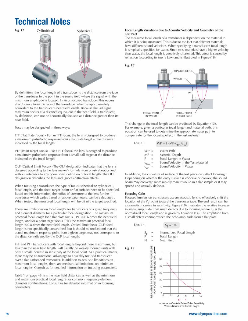
Focusing ConfigurationsImmersion transducers are available in three different configurations: unfocused (“flat”), spherically (“spot”) focused, and cylindrically (“line”) focused. Focusing is accomplished by either the addition of a lens or by curving the element itself. The addition of a lens is the most common way to focus a transducer.

An unfocused transducer may be used in general applications or for penetration of thick materials. A spherically focused transducer is commonly used to improve sensitivity to small flaws and a cylindrical focus is typically used in the inspection of tubing or bar stock. Examples of spherical and cylindrical focusing are shown in Figure (17).

Technical Notes

�

45

www.olympus-ims.com

Fig. 17

By definition, the focal length of a transducer is the distance from the face of the transducer to the point in the sound field where the signal with the maximum amplitude is located. In an unfocused transducer, this occurs at a distance from the face of the transducer which is approximately equivalent to the transducer’s near field length. Because the last signal maximum occurs at a distance equivalent to the near field, a transducer, by definition, can not be acoustically focused at a distance greater than its near field.

Focus may be designated in three ways:

FPF (Flat Plate Focus) - For an FPF focus, the lens is designed to produce a maximum pulse/echo response from a flat plate target at the distance indicated by the focal length

PTF (Point Target Focus) - For a PTF focus, the lens is designed to produce a maximum pulse/echo response from a small ball target at the distance indicated by the focal length

OLF (Optical Limit Focus) - The OLF designation indicates that the lens is designed according to the lens maker’s formula from physical optics and without reference to any operational definition of focal length. The OLF designation describes the lens and ignores diffraction effects.

When focusing a transducer, the type of focus (spherical or cylindrical), focal length, and the focal target (point or flat surface) need to be specified. Based on this information, the radius of curvature of the lens for the transducer which varies based on above parameters, can be calculated . When tested, the measured focal length will be off of the target specified.

There are limitations on focal lengths for transducers of a given frequency and element diameter for a particular focal designation. The maximum practical focal length for a flat plate focus (FPF) is 0.6 times the near field length, and for a point target focus (PTF) the maximum practical focal length is 0.8 times the near field length. Optical limit focus (OLF) focal length is not specifically constrained, but it should be understood that the actual maximum response point from a given target may not correspond to the distance indicated by the OLF focal length.

FPF and PTF transducers with focal lengths beyond these maximums, but less than the near field length, will usually be weakly focused units with only a small increase in sensitivity at the focal point. As a practical matter, there may be no functional advantage to a weakly focused transducer over a flat, unfocused transducer. In addition to acoustic limitations on maximum focal lengths, there are mechanical limitations on minimum focal lengths. Consult us for detailed information on focusing parameters.

Table 1 on page 48 lists the near field distances as well as the minimum and maximum practical focal lengths for common frequency-element diameter combinations. Consult us for detailed information in focusing parameters.

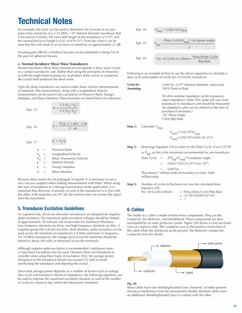
Focal Length Variations due to Acoustic Velocity and Geometry of the Test PartThe measured focal length of a transducer is dependent on the material in which it is being measured. This is due to the fact that different materials have different sound velocities. When specifying a transducer’s focal length it is typically specified for water. Since most materials have a higher velocity than water, the focal length is effectively shortened. This effect is caused by refraction (according to Snell’s Law) and is illustrated in Figure (18).

Fig. 18

This change in the focal length can be predicted by Equation (13). For example, given a particular focal length and material path, this equation can be used to determine the appropriate water path to compensate for the focusing effect in the test material.

Eqn. 13

WP = Water PathMP = Material DepthF = Focal Length in Waterctm = Sound Velocity in the Test Materialcw = Sound Velocity in Water

In addition, the curvature of surface of the test piece can affect focusing. Depending on whether the entry surface is concave or convex, the sound beam may converge more rapidly than it would in a flat sample or it may spread and actually defocus.

Focusing GainFocused immersion transducers use an acoustic lens to effectively shift the location of the Y0

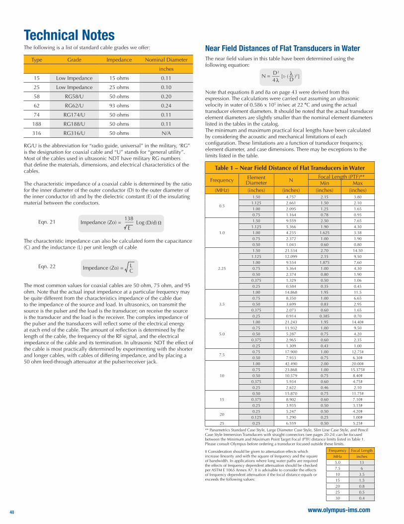
+ point toward the transducer face. The end result can be a dramatic increase in sensitivity. Figure (19) illustrates the relative increase in signal amplitude from small defects due to focusing where SF is the normalized focal length and is given by Equation (14). The amplitude from a small defect cannot exceed the echo amplitude from a flat plate.

Eqn. 14

SF = Normalized Focal LengthF = Focal LengthN = Near Field

Fig. 19

Technical NotesSphericalCylindrical

46

For example, the chart can be used to determine the increase in on-axis pulse-echo sensitivity of a 2.25 MHz, 1.0" element diameter transducer that is focused at 4 inches. The near field length of this transducer is 9.55", and the normalized focal length is 0.42 (4.0"/9.55"). From the chart it can be seen that this will result in an increase in sensitivity of approximately 21 dB.

Focusing gain (dB) for cylindrical focuses can be estimated as being 3/4 of the gain for spherical focuses.

e. Normal Incidence Shear Wave TransducersNormal Incidence Shear Wave transducers incorporate a shear wave crystal in a contact transducer case. Rather than using the principles of refraction, as with the angle beam transducers, to produce shear waves in a material, the crystal itself produces the shear wave.

Typically these transducers are used to make shear velocity measurements of materials. This measurement, along with a longitudinal velocity measurement can be used in the calculation of Poisson’s Ratio, Young’s Modulus, and Shear Modulus. These formulas are listed below for reference.

Eqn. 15

Eqn. 16

Eqn. 17

s = Poisson’s RatioVL = Longitudinal VelocityVT = Shear (Transverse) Velocityr = Material Density

E = Young’s Modulus

G = Shear Modulus

Because shear waves do not propagate in liquids, it is necessary to use a very viscous couplant when making measurements with these. When using this type of transducer in a through transmission mode application, it is important that direction of polarity of each of the transducers is in line with the other. If the polarities are 90° off, the receiver may not receive the signal from the transmitter.

5. Transducer Excitation GuidelinesAs a general rule, all of our ultrasonic transducers are designed for negative spike excitation. The maximum spike excitation voltages should be limited to approximately 50 volts per mil of piezoelectric transducer thickness. Low frequency elements are thick, and high frequency elements are thin. A negative-going 600 volt fast rise time, short duration, spike excitation can be used across the terminals on transducers 5.0 MHz and lower in frequency. For 10 MHz transducers, the voltage used across the terminals should be halved to about 300 volts as measured across the terminals.

Although negative spike excitation is recommended, continuous wave or tone burst excitations may be used. However there are limitations to consider when using these types of excitation. First, the average power dissipation to the transducer should not exceed 125 mW to avoid overheating the transducer and depoling the crystal.

Since total average power depends on a number of factors such as voltage, duty cycle and transducer electrical impedance, the following equations can be used to estimate the maximum excitation duration as well as the number of cycles in a burst to stay within the total power limitation:

Eqn. 18

Eqn. 19

Eqn. 20

Following is an example of how to use the above equations to calculate a duty cycle and number of cycles for a V310-SU transducer.

V310-SU 5.0M Hz, 0.25" element diameter, unfocusedAssuming: 100 V Peak-to-Peak 50 ohm nominal impedance at the transducer

input impedance (Note: This value will vary from transducer to transducer and should be measured. An impedance plot can be ordered at the time of purchase if necessary.)

-45° Phase Angle 5 kHz Rep Rate

Step 1: Calculate Vrms Vrms=1/2(0.707)Vp-p Vrms=1/2(0.707)(100)=35.35 V

Step 2: Rearrange Equation (19) to solve for the Duty Cycle. Use 0.125 W

as Ptot, as this is the maximum recommended for any transducer.

Duty Cycle = Z*Ptot/(Vrms)2*cos(phase angle)

= (50)(0.125)/(35.35)2*(cos -45°)

= 0.007s/s This means 7 milliseconds of excitation in every 1000

milliseconds.

Step 3: Number of cycles in the burst can now be calculated from Equation (20).

No. Of Cycles in Burst = (Freq.)(Duty Cycle) Rep Rate = (5*106)*(0.007)/(5*103) = 7

6. CablesThe inside of a cable is made of three main components. They are the conductor, the dielectric, and shield/braid. These components are then surrounded by an outer protective jacket. Figure (20) shows a cross-sectional view of a typical cable. The conductor acts as the positive connection of the cable while the shield acts as the ground. The dielectric isolates the conductor from the shield.

Fig. 20Most cables have one shielding/braided layer. However, to better prevent electrical interference from the environment double shielded cables have an additional shielding/braided layer in contact with the other.

Technical Notes

47

www.olympus-ims.com

The following is a list of standard cable grades we offer:

Type Grade Impedance Nominal Diameter

inches

15 Low Impedance 15 ohms 0.11

25 Low Impedance 25 ohms 0.10

58 RG58/U 50 ohms 0.20

62 RG62/U 93 ohms 0.24

74 RG174/U 50 ohms 0.11

188 RG188/U 50 ohms 0.11

316 RG316/U 50 ohms N/A

RG/U is the abbreviation for “radio guide, universal” in the military, ‘RG” is the designation for coaxial cable and “U” stands for “general utility”. Most of the cables used in ultrasonic NDT have military RG numbers that define the materials, dimensions, and electrical characteristics of the cables.

The characteristic impedance of a coaxial cable is determined by the ratio for the inner diameter of the outer conductor (D) to the outer diameter of the inner conductor (d) and by the dielectric constant (E) of the insulating material between the conductors.

Eqn. 21

The characteristic impedance can also be calculated form the capacitance (C) and the inductance (L) per unit length of cable

Eqn. 22

The most common values for coaxial cables are 50 ohm, 75 ohm, and 95 ohm. Note that the actual input impedance at a particular frequency may be quite different from the characteristics impedance of the cable due to the impedance of the source and load. In ultrasonics, on transmit the source is the pulser and the load is the transducer; on receive the source is the transducer and the load is the receiver. The complex impedance of the pulser and the transducers will reflect some of the electrical energy at each end of the cable. The amount of reflection is determined by the length of the cable, the frequency of the RF signal, and the electrical impedance of the cable and its termination. In ultrasonic NDT the effect of the cable is most practically determined by experimenting with the shorter and longer cables, with cables of differing impedance, and by placing a 50 ohm feed-through attenuator at the pulser/receiver jack.

Technical Notes

Table 1 – Near Field Distance of Flat Transducers in Water

Frequency Element Diameter N

Focal Length (PTF)**Min Max

(MHz) (inches) (inches) (inches) (inches)

0.5

1.50 4.757 2.15 3.80

1.125 2.661 1.50 2.10

1.00 2.095 1.25 1.65

0.75 1.164 0.78 0.93

1.0

1.50 9.559 2.50 7.65

1.125 5.366 1.90 4.30

1.00 4.235 1.625 3.38

0.75 2.372 1.00 1.90

0.50 1.043 0.60 0.80

2.25

1.50 21.534 2.70 14.50

1.125 12.099 2.15 9.50

1.00 9.554 1.875 7.60

0.75 5.364 1.00 4.30

0.50 2.374 0.80 1.90

0.375 1.329 0.50 1.06

0.25 0.584 0.35 0.45

3.5

1.00 14.868 1.95 11.5

0.75 8.350 1.00 6.65

0.50 3.699 0.83 2.95

0.375 2.073 0.60 1.65

0.25 0.914 0.385 0.70

5.0

1.00 21.243 1.95 14.40‡

0.75 11.932 1.00 9.50

0.50 5.287 0.75 4.20

0.375 2.965 0.60 2.35

0.25 1.309 0.43 1.00

7.50.75 17.900 1.00 12.75‡

0.50 7.933 0.75 6.30‡

10

1.00 42.490 2.00 20.00‡

0.75 23.868 1.00 15.375‡

0.50 10.579 0.75 8.40‡

0.375 5.934 0.60 4.75‡

0.25 2.622 0.46 2.10

15

0.50 15.870 0.75 11.75‡

0.375 8.902 0.60 7.10‡

0.25 3.935 0.50 3.15‡

200.25 5.247 0.50 4.20‡

0.125 1.290 0.25 1.00‡

25 0.25 6.559 0.50 5.25‡

** Panametrics Standard Case Style, Large Diameter Case Style, Slim Line Case Style, and Pencil Case Style Immersion Transducers with straight connectors (see pages 20-24) can be focused between the Minimum and Maximum Point Target Focal (PTF) distance limits listed in Table 1. Please consult Olympus before ordering a transducer focused outside these limits.

‡ Consideration should be given to attenuation effects which increase linearity and with the square of frequency and the square of bandwidth. In applications where long water paths are required the effects of frequency dependent attenuation should be checked per ASTM E 1065 Annex A7. It is advisable to consider the effects of frequency dependent attenuation if the focal distance equals or exceeds the following values:

Frequency Focal Length

MHz inches

5.0 13

7.5 6

10 3.5

15 1.5

20 0.8

25 0.5

30 0.4

Near Field Distances of Flat Transducers in WaterThe near field values in this table have been determined using the following equation:

Note that equations 8 and 8a on page 43 were derived from thisexpression. The calculations were carried out assuming an ultrasonic velocity in water of 0.586 x 105 in/sec at 22 °C and using the actual transducer element diameters. It should be noted that the actual transducer element diameters are slightly smaller than the nominal element diameters listed in the tables in the catalog. The minimum and maximum practical focal lengths have been calculated by considering the acoustic and mechanical limitations of each configuration. These limitations are a function of transducer frequency, element diameter, and case dimensions. There may be exceptions to the limits listed in the table.

48

Table 2 – Acoustic Properties of Materials

Material Longitudinal Velocity

ShearVelocity

Acoustic Impedance

(in./ms)* (m/s) (in./ms)* (m/s) (Kg/m2s x 106)Acrylic resin (Perspex) 0.107 2,730 0.056 1,430 3.22

Aluminum 0.249 6,320 0.123 3,130 17.06

Beryllium 0.508 12,900 0.350 8,880 23.5

Brass, naval 0.174 4,430 0.083 2,120 37.30

Cadmium 0.109 2,780 0.059 1,500 24.02

Columbium 0.194 4,920 0.083 2,100 42.16

Copper 0.183 4,660 0.089 2,260 41.61

Glycerine 0.076 1,920 — — 2.42

Gold 0.128 3,240 0.047 1,200 62.60

Inconel 0.29 5,820 0.119 3,020 49.47

Iron 0.232 5,900 0.127 3,230 45.43

Iron, cast

(slow) 0.138 3,500 0.087 2,200 25.00

(fast) 0.220 5,600 0.126 3,220 40.00

Lead 0.085 2,160 0.028 700 24.49

Manganese 0.183 4,660 0.093 2,350 34.44

Mercury 0.057 1,450 — — 19.66

Molybdenum 0.246 6,250 0.132 3,350 63.75

Motor Oil (SAE 20 or 30) 0.069 1,740 — — 1.51

Nickel, pure 0.222 5,630 0.117 2,960 49.99

Platinum 0.156 3,960 0.066 1,670 84.74

Polyamide, (nylon, Perlon)

(slow) 0.087 2,200 0.043 1,100 .40

(fast) 0.102 2,600 0.047 1,200 3.10

Polystyrene 0.092 2,340 — — 2.47

Polyvinylchloride, PVC, hard 0.094 2,395 0.042 1,060 3.35

Silver 0.142 3,600 0.063 1,590 37.76

Steel, 1020 0.232 5,890 0.128 3,240 45.63

Steel, 4340 0.230 5,850 0.128 3,240 45.63

Steel, 302 0.223 5,660 0.123 3,120 45.45

Austenitic stainless Steel, 347 0.226 5,740 0.122 3,090 45.40

Austenitic stainless Tin 0.131 3,320 0.066 1,670 24.20

Titanium, Ti 150A 0.240 6,100 0.123 3,120 27.69

Tungsten 0.204 5,180 0.113 2,870 99.72

Uranium 0.133 3,370 0.078 1,980 63.02

Water (20°C) 0.058 1,480 — — 1.48

Zinc 0.164 4,170 0.095 2,410 29.61

Zirconium 0.183 4,650 0.089 2,250 30.13

* Conversion Factor: 1 m/s = 3.937 x 10 -5 in/μSSource: Nondestructive Testing Handbook 2nd Edition Volume 7Ultrasonic Testing ASNT 1991 ed Paul McIntire

www.olympus-ims.com

info@olympusNDT.com

48 Woerd Avenue, Waltham, MA 02453, USA, Tel.: (1) 781-419-390012569 Gulf Freeway, Houston, TX 77034, USA, Tel.: (1) 281-922-9300

505, boul. du Parc-Technologique, Québec (Québec) G1P 4S9, Tel.: (1) 418-872-11551109 78 Ave, Edmonton (Alberta) T6P 1L8

Stock Road • Southend-on-Sea • Essex • SS2 5QH • UK

OLYMPUS SINGAPORE PTE. LTD.491B River Valley Road 12-01/04, Valley Point Office Tower, 248373 • Singapore

OLYMPUS AUSTRALIA PTY. LTD.PO Box 985 • Mount Waverley, VIC 3149 • Australia

Pana_UT_EN_201012 • Printed in USA • Copyright © 2011 by Olympus NDT.*All specifications are subject to change without notice. All brands are trademarks or registered trademarks of their respective owners.

isISO9001/ISO14001certified.