Embed Size (px)
Citation preview
NONUNIFORM MEMBRANES IN CAPACITIVEMICROMACHINED ULTRASONIC TRANSDUCERS
a thesis
submitted to the department of electrical and
electronics engineering
and the institute of engineering and science
of bilkent university
in partial fulfillment of the requirements
for the degree of
master of science
By
Muhammed N. Senlik
January 28, 2005
I certify that I have read this thesis and that in my opinion it is fully adequate,
in scope and in quality, as a thesis for the degree of Master of Science.
Prof. Dr. Abdullah Atalar (Supervisor)
I certify that I have read this thesis and that in my opinion it is fully adequate,
in scope and in quality, as a thesis for the degree of Master of Science.
Prof. Dr. Hayrettin Koymen
I certify that I have read this thesis and that in my opinion it is fully adequate,
in scope and in quality, as a thesis for the degree of Master of Science.
Assoc. Prof. Dr. Ahmet Oral
Approved for the Institute of Engineering and Science:
Prof. Dr. Mehmet BarayDirector of the Institute Engineering and Science
ii

in loving memory of my mother
iii
ABSTRACT
NONUNIFORM MEMBRANES IN CAPACITIVEMICROMACHINED ULTRASONIC TRANSDUCERS
Muhammed N. Senlik
M.S. in Electrical and Electronics Engineering
Supervisor: Prof. Dr. Abdullah Atalar
January 28, 2005
Capacitive micromachined ultrasonic transducers (cMUT) are used to receive and
transmit ultrasonic signals. The device is constructed from many small, in the
order of microns, circular membranes, which are connected in parallel. When
they are immersed in water, the bandwidth of the cMUT is limited by the mem-
brane’s second resonance frequency, which causes an increase in the mechanical
impedance of the membrane. In this thesis, we propose a new membrane shape to
shift the second resonance frequency to higher values, in addition to keeping the
impedance of the membrane as small as possible. The structure consists of a very
thin membrane with a rigid mass at the center. The stiffness of the central region
moves the second resonance to a higher frequency. This membrane configuration
is shown to work better compared to conventionally used uniform membranes
during both reception and transmission. The improvement in the bandwidth is
more than %30 with an increase in the gain.
Keywords: Capacitive micromachined ultrasonic transducer, cMUT, nonuniform
membrane.
iv
OZET
KAPASITIF MIKRO-ISLENMIS ULTRASONIKCEVIRICILERDE DUZGUN OLMAYAN ZARLAR
Muhammed N. Senlik
Elektrik ve Elektronik Muhendisligi, Yuksek Lisans
Tez Yoneticisi: Prof. Dr. Abdullah Atalar
28 Ocak 2005
Kapasitif mikro-islenmis ultrasonik ceviriciler (kMUC), ultrasonik sinyallerin
alımında ve yollanmasında kullanılırlar. Cihaz mikron mertebesindeki bircok ufak
zarın paralel baglanmasıyla olusturulur. Suda calıstırıldıklarında, kMUC’un bant
genisligi, zarın mekanik empedansının artmasına sebep olan, zarın ikinci rezo-
nans frekansı ile sınırlıdır. Bu tezde ikinci rezonans frekansını zarın empedansını
mumkun oldugunca ufak tutarak daha yukarı cıkaran yeni bir zar sekli oneriyoruz.
Yapı ortasında sert bir kutle olan cok ince bir zardan olusmaktadır. Ortadaki
kısmın sertligi ikinci rezonansı daha yuksek frekanslara cıkarmaktadır. Bu zar
yapısının alma ve yollama acısından su an kullanılmakta olan zarlardan daha
iyi oldugu gosterilmistir. Bant genisligindeki iyilesme kazancta artısla birlikte
%30’dan daha fazladır.
Anahtar sozcukler : Kapasitif mikro-islenmis ultrasonik cevirici, kMUC, duzgun
olmayan zar.
v
ACKNOWLEDGEMENTS
I would like to express my sincere gratitude to Dr. Abdullah Atalar for his su-
pervision, guidance and encouragement through the development of this thesis.
I would like to thank to the members of my thesis jury for reading the
manuscript and commenting on the thesis.
Endless thanks to Selim for useful discussions, always coming with a new idea
to each meeting and the brilliant solutions to the problems we met.
Many thanks to my officemate, Onur Bakır. And I would like to express my
sincere gratitude to the following people: Bozbey, Vahit, analog mates Mehmet
and Cagrı, Ferhat (a.k.a. kırmızı), Ali Rıza (a.k.a. karanfil), Durukal, Hakan,
Namık, Kamer, Apo, Deligoz.
Without my parents and aunt, this work would never be possible.
Finally, one another person, my brother, Servet deserves special thanks. Al-
though I am the elder one, he was both a father and a mother for me since he
came to Bilkent. Thanks for always being there.
vi
Contents
1 INTRODUCTION 1
2 FUNDAMENTALS OF cMUT 3
2.1 cMUTs . . . . . . . . . . . . . . . . . . . . . . . . . . . . . . . . . 3
2.2 Operating Principles and Regimes . . . . . . . . . . . . . . . . . . 5
2.2.1 Conventional Regime . . . . . . . . . . . . . . . . . . . . . 6
2.2.2 Collapsed Regime . . . . . . . . . . . . . . . . . . . . . . . 7
2.3 Mathematical Formulation . . . . . . . . . . . . . . . . . . . . . . 7
2.4 Nonuniform Membranes . . . . . . . . . . . . . . . . . . . . . . . 10
3 MODELING 12
3.1 Small Signal Equivalent Circuit . . . . . . . . . . . . . . . . . . . 12
3.2 Finite Element Model . . . . . . . . . . . . . . . . . . . . . . . . . 15
4 RESULTS AND DISCUSSIONS 19
4.1 Electrode Patterning . . . . . . . . . . . . . . . . . . . . . . . . . 20
vii
CONTENTS viii
4.2 Resonance Frequency Change . . . . . . . . . . . . . . . . . . . . 21
4.3 Receive Mode . . . . . . . . . . . . . . . . . . . . . . . . . . . . . 25
4.4 Transmit Mode . . . . . . . . . . . . . . . . . . . . . . . . . . . . 32
5 CONCLUSION 36
A 38
A.1 Solution Of Mason’s Differential Equation . . . . . . . . . . . . . 38
A.2 Derivation Of Operation Parameters . . . . . . . . . . . . . . . . 40
B Finite Element Simulation 43
B.1 Static Analysis . . . . . . . . . . . . . . . . . . . . . . . . . . . . 44
B.2 Dynamic Analysis . . . . . . . . . . . . . . . . . . . . . . . . . . . 46
C MATERIAL PARAMETERS 47
List of Figures
2.1 3D view of a single cMUT cell fabricated with sacrificial layer method. 4
2.2 (a) Deflection of the center of the membrane with respect to the
applied voltage. Arrows indicate the direction of movement as the
voltage is changed. (b) Membrane shapes for various voltages. Re-
gion denoted as ‘1’ is before collapse and two membrane shapes at
voltages just before collapse and after snap-back is drawn. Region
‘2’ is after collapse and membrane shapes are drawn for just after
collapse and before snap-back [1]. . . . . . . . . . . . . . . . . . . 5
2.3 2D view of a single cMUT cell fabricated with sacrificial layer method. 6
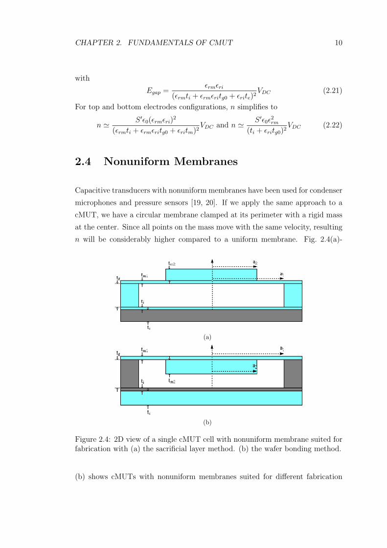
2.4 2D view of a single cMUT cell with nonuniform membrane suited
for fabrication with (a) the sacrificial layer method. (b) the wafer
bonding method. . . . . . . . . . . . . . . . . . . . . . . . . . . . 10
2.5 First order model, a series combination of a spring and a mass
system. . . . . . . . . . . . . . . . . . . . . . . . . . . . . . . . . . 11
3.1 Mason model (a) for a cMUT operating as a receiver excited by
the acoustical source (FS, ZaS) to drive the electrical load resis-
tance of the receiver circuitry (RS) (b) for a cMUT operating as a
transmitter excited by a voltage source (VS) to drive the acoustic
impedance of the immersion medium (ZaS). S is the area of the
transducer . . . . . . . . . . . . . . . . . . . . . . . . . . . . . . . 13
ix
LIST OF FIGURES x
3.2 Circular membrane meshed with quadrilateral elements clamped
at its perimeter. . . . . . . . . . . . . . . . . . . . . . . . . . . . . 15
3.3 (a) Maximum deflection of membrane under sinusoidally vary-
ing uniform pressure (for 100 Pa at 2.5 MHz). (b) Mechanical
impedance of the membrane. . . . . . . . . . . . . . . . . . . . . . 16
3.4 Iterative solution of membrane shape under various operating volt-
ages (a) Converged solution at 120 V. (b) Un-converged (collapsed)
solution at 130 V in conventional regimes. (c) Converged solution
at 130 V in collapsed regime. . . . . . . . . . . . . . . . . . . . . . 17
3.5 cMUT model used in simulations. . . . . . . . . . . . . . . . . . . 18
4.1 Change of Vcol, C0 and n with respect to the electrode size for the
uniform membrane. . . . . . . . . . . . . . . . . . . . . . . . . . . 21
4.2 Change of Vcol, C0 and n with respect to the electrode size for the
nonuniform membrane. . . . . . . . . . . . . . . . . . . . . . . . . 22
4.3 Modal shapes of the uniform membrane at fr (upper one) and fa
(lower one). . . . . . . . . . . . . . . . . . . . . . . . . . . . . . . 22
4.4 Change of fr and fa of the uniform membrane with respect to tm
for constant a. . . . . . . . . . . . . . . . . . . . . . . . . . . . . . 23
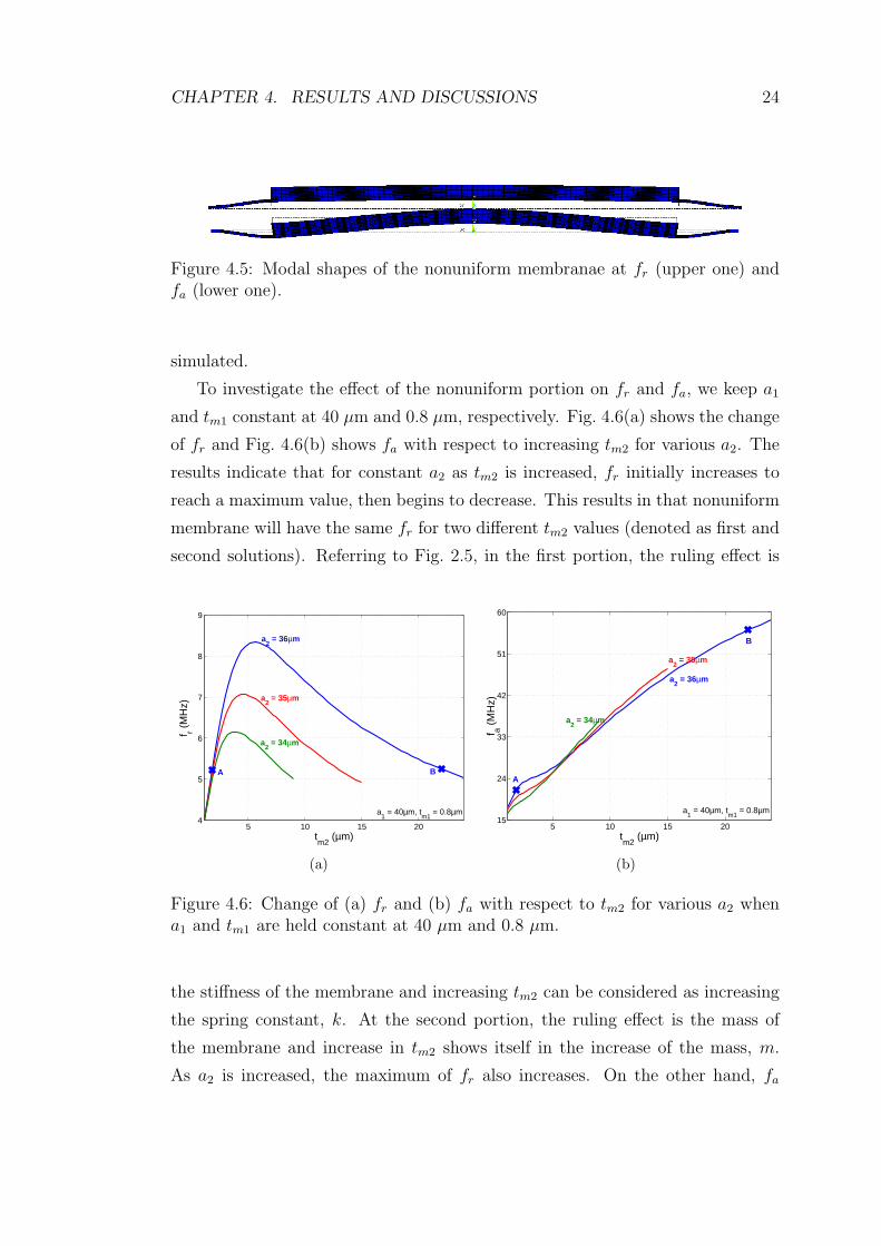
4.5 Modal shapes of the nonuniform membranae at fr (upper one) and
fa (lower one). . . . . . . . . . . . . . . . . . . . . . . . . . . . . . 24
4.6 Change of (a) fr and (b) fa with respect to tm2 for various a2 when
a1 and tm1 are held constant at 40 µm and 0.8 µm. . . . . . . . . 24
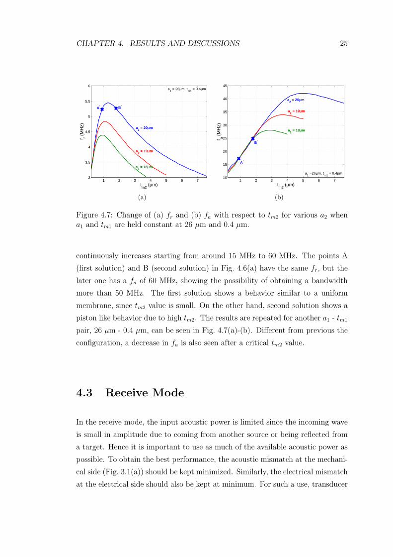
4.7 Change of (a) fr and (b) fa with respect to tm2 for various a2 when
a1 and tm1 are held constant at 26 µm and 0.4 µm. . . . . . . . . 25
LIST OF FIGURES xi
4.8 (a) Definition of figure of merit for the receive mode, MR. (b)
Transducer gain, GT , and the mechanical impedance of the mem-
brane, Zm, (spring softening effect is included) with respect to
frequency. . . . . . . . . . . . . . . . . . . . . . . . . . . . . . . . 26
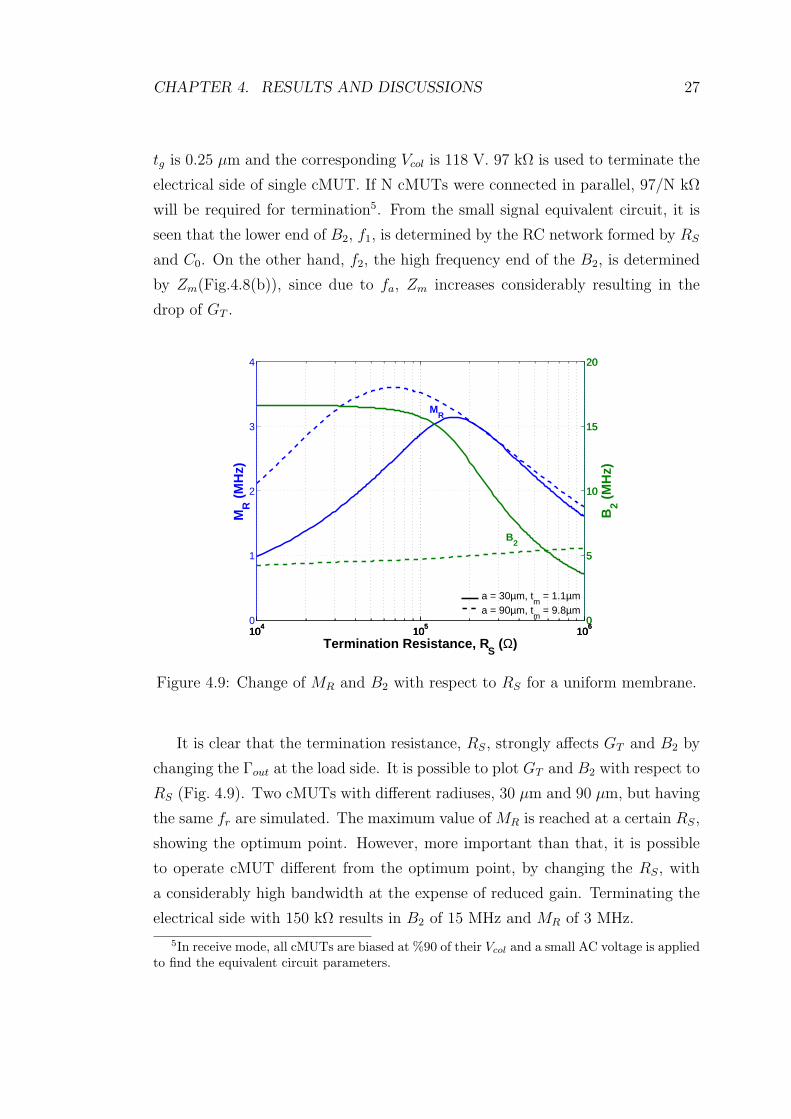
4.9 Change of MR and B2 with respect to RS for a uniform membrane. 27
4.10 Change of MR and B2 with respect to electrode radius for a uniform
membrane. . . . . . . . . . . . . . . . . . . . . . . . . . . . . . . . 28
4.11 Change of MR and B2 with respect to a for a uniform membrane. 29
4.12 (a) Change of MR and B2 with respect to RS for the nonuniform
membranes denoted as A and B in Fig. 4.6(a). (b) Zm of the points
A and B (spring softening effect is not included). . . . . . . . . . 30
4.13 Nonuniform membrane fabricated with the sacrificial layer method. 30
4.14 Change of MR and B2 with respect to RS for the nonuniform mem-
branes denoted as A’ and B’ in Fig. 4.7(a). . . . . . . . . . . . . . 31
4.15 Change of MR and B2 with respect to electrode radius for a nonuni-
form membrane. . . . . . . . . . . . . . . . . . . . . . . . . . . . . 32
4.16 Change of MR and B2 with respect to a1 corresponding to the (a)
first solution. (b) second solution. . . . . . . . . . . . . . . . . . . 33
4.17 Definition of figure of merit for the transmit mode. . . . . . . . . 33
4.18 (a) Change of MT and B1 with respect to the electrode radius. (b)
Change of MT and B1 with respect to a for a uniform membrane. 34
4.19 Change of MT and B1 with respect to (a) the electrode radius (b)
a1 corresponding to the first solution. (c) a1 corresponding to the
second solution. . . . . . . . . . . . . . . . . . . . . . . . . . . . . 35
B.1 Application of (a) voltages and (b) electrostatic forces to FEM . . 44

Chapter 1
INTRODUCTION
Ultrasound, a rich field of study, found many applications in diverse areas rang-
ing from nondestructive evaluation (NDE) to process control, cleaning to imag-
ing [2, 3]. In most of the applications, piezoelectric materials are the first choice
for constructing transducers [4]. In imaging applications, they work well in terms
of both bandwidth and gain when the surrounding medium is solid. However,
when they are immersed in a light medium1 such as air and water, they have
typically a low bandwidth due to the mismatch in acoustic impedances2 and lack
of proper matching layers, but still present high gain.
Recent advances in micromachining technology enabled the invention of ca-
pacitive micromachined ultrasonic transducer (cMUT), first reported in [6]. The
device is constructed from a circular silicon nitride membrane suspended over sili-
con substrate with a small spacing, in sub-micrometer range, to form a capacitor.
The impedance of the membrane is chosen to be low compared to the impedance
of the immersion medium to increase the possibility of obtaining high bandwidth.
However, they have small turns ratio3 resulting in a small gain.
1Light medium is used for a medium having low acoustic impedance, which is defined asZa = Vaρ where Va is the speed of sound in the medium and ρ is the density of the medium.
2Air and water have acoustic impedances of 400 kg/m2s and 1.5 × 10⁶ kg/m2s, whereas atypical transducer impedance is 10× 106 kg/m2s [5].
3Turns ratio is used to determine the amount of conversion between the average velocity, amechanical quantity, and the current, an electrical quantity, in an electromechanical system.
1
CHAPTER 1. INTRODUCTION 2
In a recent work [7], performance measures in terms of a gain-bandwidth prod-
uct for both transmit and receive modes are defined. It is shown that a cMUT
immersed in water can be optimized for both high gain and bandwidth for a given
frequency range.
In this work, we show that the bandwidth of cMUT is limited by the antires-
onance frequency of the membrane, which causes an increase in the membrane
impedance. We find that use of a nonuniform membrane, a membrane with a
rigid mass at the center, results in higher turns ratio and shifts the antiresonance
frequency of the membrane to higher values without increasing the membrane
impedance. Results are obtained for both uniform and nonuniform membranes
for reception and transmission. They indicate that the nonuniform membranes
are advantageous compared to the uniform ones in many aspects.
Chapter 2 gives the fundamentals and basic operation principles of cMUT.
Chapter 3 introduces the tools that are used in modeling and simulations. Chap-
ter 4 presents the results for various membrane configurations at different oper-
ation modes. The last chapter concludes this work.
Chapter 2
FUNDAMENTALS OF cMUT
In this chapter; capacitive micromachined ultrasonic transducer (cMUT) and
its basic operation principles for different regimes are introduced. Underlying
theory for cMUT is formulated. The chapter ends with some remarks regarding
nonuniform membranes.
2.1 cMUTs
An ultrasonic transducer is used to receive and transmit ultrasonic signals. Most
ultrasonic transducers are made up of piezoelectric materials [4]. When an electric
field is applied to such a material, it changes its shape in response to applied field,
hence creates an ultrasonic wave. Similarly, when its shape is changed, the elec-
tric field inside the material also changes, which corresponds to the detection of
an ultrasonic wave. However, in terms of bandwidth in a light immersion medium
such as air or water, integration with surrounding electronics and construction
of transducer arrays, they have several drawbacks. Capacitive micromachined
ultrasonic transducer (cMUT), first reported in [6], has advantages over their
piezoelectric counterpart in terms of above considerations [8, 9, 10]. However,
piezoelectric transducers have still higher gain compared to cMUTs due to their
higher electromechanical coupling coefficient, k2T [4, 11].
3

CHAPTER 2. FUNDAMENTALS OF CMUT 4
Fig. 2.1 shows 3D view of a single cMUT cell fabricated with the sacrificial
layer method. The whole structure lies on silicon substrate, whose top is highly
doped, which also acts as the ground electrode. Vibrating silicon nitride mem-
brane is supported by silicon nitride stands. A metal (aluminum or gold) inside
the membrane (whose position may vary) forms the top electrode. There is a
thin silicon nitride insulator region above the substrate to prevent short circuits
between the electrodes when membrane collapses. The gap that is formed inside
the structure may or may not be sealed depending on the application. To in-
crease the directivity and amount of received/transmitted power, many cMUTs
are connected in parallel to form an array [12]. To fabricate cMUTs, there are
two major methods, which are sacrificial layer [13, 14] and wafer bonding [15]
methods. In wafer bonding method, silicon is used as the membrane material
and silicon oxide is used as the insulator and stand.
Figure 2.1: 3D view of a single cMUT cell fabricated with sacrificial layer method.
When a voltage is applied between the electrodes, regardless of the polarity,
the membrane will deflect towards the substrate due to the attractive electro-
static forces. As the voltage is increased, the slope of the voltage-deflection curve
also increases showing the increase of sensitivity with the applied voltage. At
a critical point denoted as collapse voltage, Vcol, the restoring forces of mem-
brane can no longer resist the electrostatic forces and membrane collapses onto
the insulator with a certain contact radius. Until the voltage is decreased to a
critical value, Vsb the membrane contacts with the insulator and then it snaps
back. Such a hysteresis behavior and membrane shapes for various voltages are
CHAPTER 2. FUNDAMENTALS OF CMUT 5
0 20 40 60 80 100 120−1
−0.9
−0.8
−0.7
−0.6
−0.5
−0.4
−0.3
−0.2
−0.1
0
Applied Voltage (V)
Max
imum
Dis
plac
emen
t (µm
)
Vcol
Vsb
(a)
0 10 20 30 40 50−1
−0.9
−0.8
−0.7
−0.6
−0.5
−0.4
−0.3
−0.2
−0.1
0
Radial Distance (µm)
Axi
al D
ispl
acem
ent (
µm)
(1) @ 123V(1) @ 64V(2) @ 123V(2) @ 64V
1
2
(b)
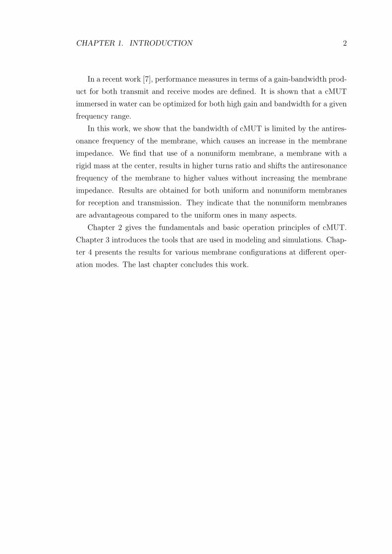
Figure 2.2: (a) Deflection of the center of the membrane with respect to theapplied voltage. Arrows indicate the direction of movement as the voltage ischanged. (b) Membrane shapes for various voltages. Region denoted as ‘1’ isbefore collapse and two membrane shapes at voltages just before collapse andafter snap-back is drawn. Region ‘2’ is after collapse and membrane shapes aredrawn for just after collapse and before snap-back [1].
shown in Fig. 2.2(a)-(b). Results are obtained for a cMUT fabricated with sac-
rificial layer method. The membrane radius and thickness are 50 µm and 1 µm,
respectively. The gap height and thickness of the insulator are 1 µm and 0.1 µm.
Such a device has a Vcol of 123 V and Vsb of 64 V.
2.2 Operating Principles and Regimes
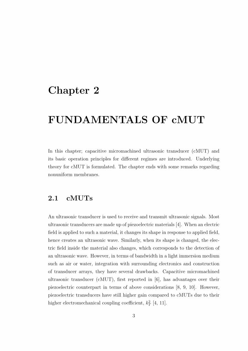
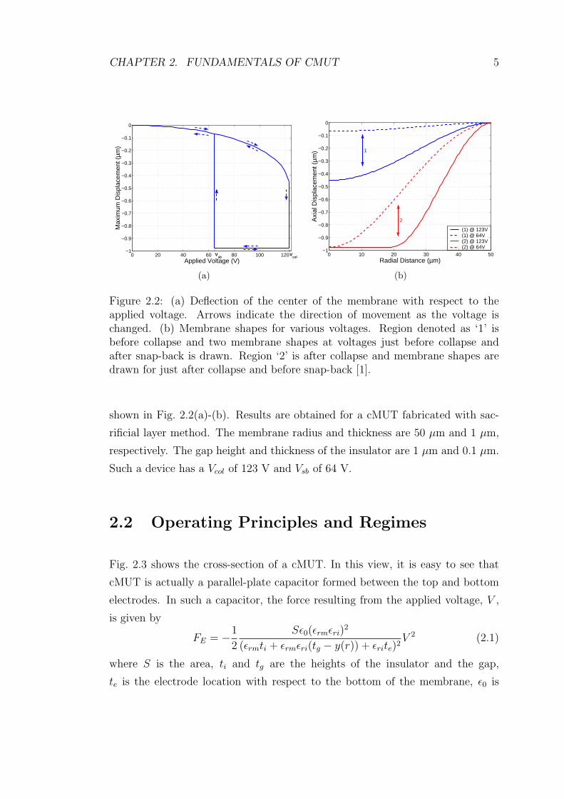
Fig. 2.3 shows the cross-section of a cMUT. In this view, it is easy to see that
cMUT is actually a parallel-plate capacitor formed between the top and bottom
electrodes. In such a capacitor, the force resulting from the applied voltage, V ,
is given by
FE = −1
2
Sε0(εrmεri)2
(εrmti + εrmεri(tg − y(r)) + εrite)2V 2 (2.1)
where S is the area, ti and tg are the heights of the insulator and the gap,
te is the electrode location with respect to the bottom of the membrane, ε0 is
CHAPTER 2. FUNDAMENTALS OF CMUT 6
Figure 2.3: 2D view of a single cMUT cell fabricated with sacrificial layer method.
the permittivity of free space, and εri and εrm are the relative permittivities of
insulator and membrane material. Since the force (Eq. 2.1) is proportional to
V 2; to avoid harmonic generation, a DC bias must be applied prior to operation.
Hence the total applied voltage will be in the form of
V (t) = VDC + VACsin(ωt) (2.2)
During the transmission, cMUT is driven with high amplitude AC voltage to
couple more power to the medium. In receive mode, it is initially biased close
to Vcol. An incoming ultrasonic wave hits and vibrates the membrane. Such a
vibration changes the total charge on the capacitor and creates a current across
it.
2.2.1 Conventional Regime
In this regime, cMUT is operated such that it doesn’t collapse [8]. Hence total
operating voltage (Eq. 2.2) must be less than Vcol. For higher sensitivity, cMUT
is operated near Vcol resulting in higher operating voltages. Although this situ-
ation is not a problem for receive mode; in transmit mode since cMUT must be
driven with high AC to couple more power to surrounding medium; a high output
pressure cannot be obtained without collapsing the membrane or increasing tg.
Despite these factors, conventional regime offers good linearity [16].
CHAPTER 2. FUNDAMENTALS OF CMUT 7
2.2.2 Collapsed Regime
This regime, recently proposed by Bayram et all. [1], leads to higher k2T than
the conventional regime. An initial voltage greater than Vcol is applied resulting
the membrane to collapse and cMUT is operated in this mode contacting with
the insulator. During the operation, total voltage (Eq. 2.2) must be greater than
Vsb to prevent cMUT to return to conventional mode. Depending on the applied
voltage, the radius of the contact between the insulator and membrane changes
and since this region is stationary, it is treated as a parasitic capacitance, which
can be very high. Despite these, the collapsed regime provides a higher output
pressure and linearity compared to the conventional regime [16].
2.3 Mathematical Formulation
cMUTs are typically fabricated in hexagonal shapes which allow close packing.
However they can be successfully approximated with circular membranes clamped
at their circumferences. The normal displacement of such a shape (Fig. 2.3)
with radius a operating in vacuum under uniform pressure obeys the differential
equation
(Y0 + T )t3m12(1− σ2)
∇4y(r, t)− tmT∇2y(r, t)− P + tmρ∂2y(r, t)
∂t2= 0 (2.3)
derived by Mason [17], where T is the residual stress, Y0 is the Young’s modulus,
σ is the Poisson’s ratio, ρ is the density of the membrane and P is the uni-
form pressure applied to the membrane. Under harmonic excitation using ejwt
notation, we obtain
(Y0 + T )t3m12(1− σ2)
∇4y(r)− tmT∇2y(r)− P − ω2tmρy(r) = 0 (2.4)
To solve the equation (explicit spatial dependence of y has been left out), we need
two boundary conditions which are
y(r)|r=a = 0 anddy(r)
dr
r=a
= 0 (2.5)
CHAPTER 2. FUNDAMENTALS OF CMUT 8
then the solution is given by
y(r) =P
ω2tmρ
[−k2J1(k2a)J0(k1r) + k1J1(k1a)J0(k2r)
−k2J1(k2a)J0(k1a) + k1J1(k1a)J0(k2a)− 1
](2.6)
where J0 and J1 are the zeroth and first order Bessel functions of the 1st kind
with
c =(Y0 + T )t2m12(1− σ2)ρ
, d =T
ρ(2.7)
and
k1 =
√−d +
√d2 + 4cω2
2c, k2 = j
√d +
√d2 + 4cω2
2c(2.8)
To complete the analysis, we have to find the mechanical impedance, Zm. The
mechanical impedance is defined as the ratio of applied uniform pressure to re-
sulting average velocity which is
Zm =P
v
= jωltρ[ ak1k2(−k2J1(k2a)J0(k1a) + k1J1(k1a)J0(k2a))
ak1k2(−k2J1(k2a)J0(k1a) + k1J1(k1a)J0(k2a))− 2(k21 − k2
2)J1(k1a)J1(k2a)
]
(2.9)
The first resonance (natural resonance) frequency, fr, of membrane is given by
fr =(2.4)2
2π
√Y0 + T
12ρ(1− σ2)
tma2
(2.10)
The static deflection of membrane can be found by setting the time deriva-
tive term of Mason’s differential equation Eq. 2.3 to 0 and solving the resulting
equation. Then, the static displacement is calculated as
y(r) =P
T
[a[J0(k3r)− J0(k3a)]
2k3J1(k3a)+
a2 − r2
4
](2.11)
with
k3 =
√T
ctmρ(2.12)
when the residual stress is neglected, T → 0, the equation simplifies to
y(r) =12P (1− σ2)
Y0t3m
[r4 + a4
64− a2r2
32
](2.13)
CHAPTER 2. FUNDAMENTALS OF CMUT 9
The membrane collapses when the deflection of the center, y(r = 0), is
y(r)|r=0 =teff
3(2.14)
where the effective gap height, teff is
teff = tg +εrmti + εrite
εrmεri
(2.15)
and at that point collapse voltage, Vcol, is
Vcol =
√128Y0t3mt3eff
36ε0(1− σ2)a4(2.16)
Shunt input capacitance, C0, is an important parameter that determines the
performance of cMUT in terms of gain and bandwidth. It is formed between the
top and bottom electrodes. It can be written in the integral form as
C0 '∫ 2π
0
∫ a+teff
0
ε0εrmεri
εrmti + εrmεri(tg − y(r)) + εriterdrdθ
' S ′ε0εrmεri
εrmti + εrmεritg0 + εrite(2.17)
The extra capacitance due to the fringing fields is included by extending the radius
from a to a+ teff [7] and S ′ is the corresponding membrane area. Approximation
is performed under the assumption that all points of membrane deflected at the
same amount which is tg − tg0. Since depending on the fabrication process; most
of the cMUTs are fabricated with electrodes on top (te = tm) or bottom (te = 0)
of their membranes; C0 of these limiting cases has great importance and is given
by
C0 ' S ′ε0εrmεri
εrmti + εrmεritg0 + εritmand C0 ' S ′εri
ti + εritg0
(2.18)
for top and bottom electrodes.
Another important parameter for cMUT is the turns ratio, n, which denotes
the conversion ratio between the electrical domain quantity, current and the me-
chanical domain one, velocity. For general case, it is given by
n =S ′ε0(εrmεri)
2
(εrmti + εrmεritg0 + εrite)2VDC (2.19)
which can also be written as the product of C0 and the electric field across the
gap, Egap, [18]
n = C0Egap (2.20)
CHAPTER 2. FUNDAMENTALS OF CMUT 10
with
Egap =εrmεri
(εrmti + εrmεritg0 + εrite)2VDC (2.21)
For top and bottom electrodes configurations, n simplifies to
n ' S ′ε0(εrmεri)2
(εrmti + εrmεritg0 + εritm)2VDC and n ' S ′ε0ε
2rm
(ti + εritg0)2VDC (2.22)
2.4 Nonuniform Membranes
Capacitive transducers with nonuniform membranes have been used for condenser
microphones and pressure sensors [19, 20]. If we apply the same approach to a
cMUT, we have a circular membrane clamped at its perimeter with a rigid mass
at the center. Since all points on the mass move with the same velocity, resulting
n will be considerably higher compared to a uniform membrane. Fig. 2.4(a)-
(a)
(b)
Figure 2.4: 2D view of a single cMUT cell with nonuniform membrane suited forfabrication with (a) the sacrificial layer method. (b) the wafer bonding method.
(b) shows cMUTs with nonuniform membranes suited for different fabrication
CHAPTER 2. FUNDAMENTALS OF CMUT 11
methods. The radius and thickness of the mass at the middle of the membrane
are a2 and (tm1 + tm2). The radius of the uniform part is a1.
Nonuniform membranes have an antiresonance frequency, fa, considerably
higher than the uniform membrane by preventing the deflections due to the second
resonance. However, Zm can easily assume very high values with a certain choices
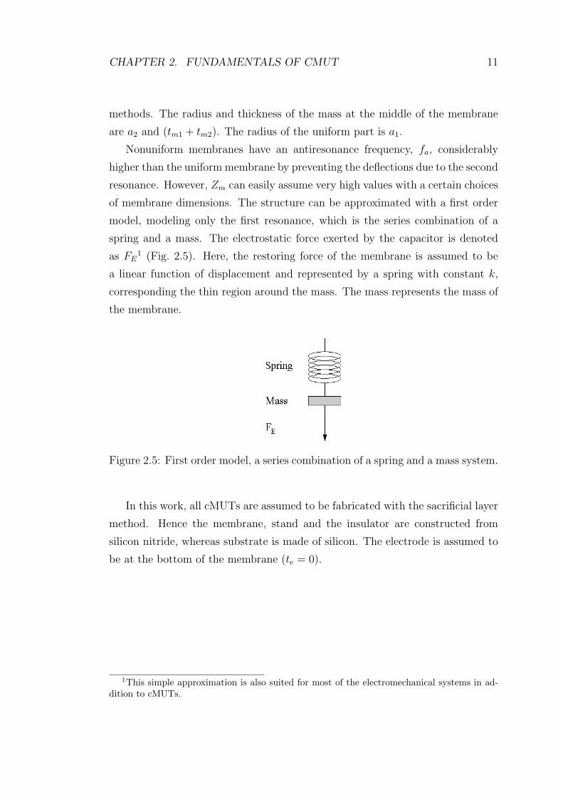
of membrane dimensions. The structure can be approximated with a first order
model, modeling only the first resonance, which is the series combination of a
spring and a mass. The electrostatic force exerted by the capacitor is denoted
as FE1 (Fig. 2.5). Here, the restoring force of the membrane is assumed to be
a linear function of displacement and represented by a spring with constant k,
corresponding the thin region around the mass. The mass represents the mass of
the membrane.
Figure 2.5: First order model, a series combination of a spring and a mass system.
In this work, all cMUTs are assumed to be fabricated with the sacrificial layer
method. Hence the membrane, stand and the insulator are constructed from
silicon nitride, whereas substrate is made of silicon. The electrode is assumed to
be at the bottom of the membrane (te = 0).
1This simple approximation is also suited for most of the electromechanical systems in ad-dition to cMUTs.
Chapter 3
MODELING
Equivalent circuits are powerful tools to predict the static and dynamic behav-
ior of electromechanical systems [21]. A small signal equivalent circuit (Mason’s
equivalent circuit) is proven to work correctly for cMUTs when operated in vac-
uum or a light medium such as air [8, 18]. The impedance of the loading medium
is treated as a lumped real impedance given by the product of the area of the
transducer with the acoustic impedance of the medium. However, such a model-
ing of the surrounding medium, if its acoustic impedance is high (as in the case
of water) is not enough and results in inaccurate modeling [22, 23].
First small signal equivalent circuit used in both transmit and receive is in-
troduced and its elements are discussed briefly. Then, the finite element model
used in simulations is described. The model is verified by comparing the results
with the theoretically expected ones.
3.1 Small Signal Equivalent Circuit
In the receive mode, cMUT is biased close to its collapse voltage for higher sen-
sitivity (Fig. 2.2(a)). When the wave hits cMUT, it causes the membrane to
vibrate. Such a vibration causes the total charge across the capacitor to change
and results in the creation of an AC current. In the transmit mode, to couple
12
CHAPTER 3. MODELING 13
more power to surrounding medium, cMUT is driven with high amplitude AC
voltage. (Usually in transmit mode, to overcome the effect of the attractive elec-
trostatic forces during the release of membrane; cMUT is only driven with square
voltage whose offset is used as bias voltage.) Such a case results in the genera-
tion of higher order harmonics and decrease the expected pressure value in the
medium. Although it is reasonable to use a large-signal equivalent circuit [24],
in this work small-signal equivalent circuit with few approximations is used to
predict the transmit behavior.
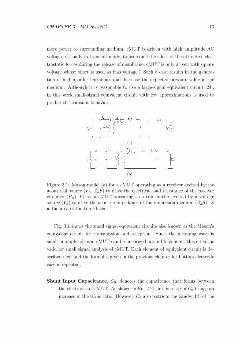
(a)
(b)
Figure 3.1: Mason model (a) for a cMUT operating as a receiver excited by theacoustical source (FS, ZaS) to drive the electrical load resistance of the receivercircuitry (RS) (b) for a cMUT operating as a transmitter excited by a voltagesource (VS) to drive the acoustic impedance of the immersion medium (ZaS). Sis the area of the transducer
Fig. 3.1 shows the small signal equivalent circuits also known as the Mason’s
equivalent circuit for transmission and reception. Since the incoming wave is
small in amplitude and cMUT can be linearized around bias point, this circuit is
valid for small signal analysis of cMUT. Each element of equivalent circuit is de-
scribed next and the formulas given in the previous chapter for bottom electrode
case is repeated.
Shunt Input Capacitance, C0, denotes the capacitance that forms between
the electrodes of cMUT. As shown in Eq. 2.21, an increase in C0 brings an
increase in the turns ratio. However, C0 also restricts the bandwidth of the
CHAPTER 3. MODELING 14
device. Hence, the relation between C0, n and bandwidth is quite complex.
For bottom electrode, it is approximated as
C0 ' S ′εri
ti + εritg0
(3.1)
Transformer and Turns Ratio, n, the heart of the device operation is per-
formed by the transformer, since it converts the electrical domain quantity,
current (I), to its analogue in the mechanical domain, which is average ve-
locity (v) (since there is a conversion between the mechanical and electrical
domains, the device is an electromechanical transducer). The ratio between
the conversion is given by the turns ratio, n,
n ' S ′ε0ε2rm
(ti + εritg0)2VDC (3.2)
Negative Capacitance, −C0/n2, as the applied DC bias is increased, the res-
onance frequency of the membrane decreases. This phenomena is called
the spring softening effect and in the equivalent circuit, by using a negative
capacitance series to mechanical impedance of the membrane, it is taken
into account.
Lumped Mechanical Impedance, ZmS, when a force is applied to the mem-
brane, it shows response to applied force. Such a force shows itself in terms
of mechanical impedance. Its definition is given by the ratio of the uniform
applied pressure to the resulting average velocity (Zm = P/v). As in the
case of piezoelectric transducers [4], the impedance can be written as in-
finite summation of series and parallel LC circuits. However, most of the
time, it is reasonable to model the impedance around the natural resonance
as series LC and antiresonance as parallel LC. Since lumped impedance is
mentioned, Zm is multiplied with transducer area, S, to find the lumped
value.
Lumped Medium Impedance, ZaS, the impedance of the surrounding
medium is treated as the real lumped impedance and given by the product
of the specific acoustic impedance, defined as the multiplication of den-
sity of the medium with the speed of sound in medium Za = ρVsonc, and
CHAPTER 3. MODELING 15
transducer area. Such a treatment doesn’t take into account the hydrody-
namic loading of medium. Although using the radiation impedance can be
a solution, as shown by [22], it is not enough.
The theoretical results are approximate and don’t take the DC bias when calcu-
lating the mechanical impedance. It is necessary to obtain the equivalent circuit
parameters by performing a finite element simulation.
3.2 Finite Element Model
Finite element simulations are required to obtain the parameters and solve the
problems of equivalent circuit discussed previously. ANSYSTM, which is a com-
mercially available finite element package capable of solving electrostatic and
structural problems, is used. First a circular membrane is modeled and solved.
The results are compared with the theoretical ones to check the validity of simu-
lations.
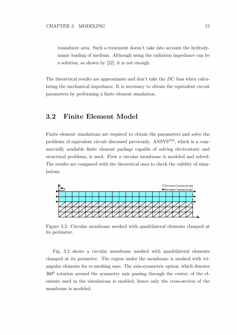
Figure 3.2: Circular membrane meshed with quadrilateral elements clamped atits perimeter.
Fig. 3.2 shows a circular membrane meshed with quadrilateral elements
clamped at its perimeter. The region under the membrane is meshed with tri-
angular elements for re-meshing ease. The axis-symmetric option, which denotes
3600 rotation around the symmetry axis passing through the center, of the el-
ements used in the simulations is enabled; hence only the cross-section of the
membrane is modeled.

CHAPTER 3. MODELING 16
The test model used for FE verification has a radius, a, and thickness, tm, of
50 µm and 1 µm. The membrane material is silicon nitride. Gap height, tg, is
1 µm. First, a sinusoidally varying uniform pressure (100 Pa), P sin(ωt) between
1.5 MHz and 2.5 MHz, is applied to the membrane. In all simulations residual
tension, T is taken to be 0. Fig. 3.3(a) shows the resulting maximum displacement
at 2.5 MHz obtained from theoretical calculations and FE simulations. There is
an excellent agrement between theoretically expected results and finite element
simulations. The second step is to determine the mechanical impedance of the
membrane. By following the definition in Eq. 2.9, a small uniform pressure, P ,
is applied to the membrane and resulting average velocity, v, is calculated. Then
P/v gives the mechanical impedance (Fig. 3.3(b)). Again there is an excellent
agrement between the theoretical results and FE simulations.
0 10 20 30 40 50
−0.5
−0.4
−0.3
−0.2
−0.1
0
Radius (µm)
Rad
ial D
ispl
acem
ent (
nm)
TheorySimulation
(a)
1.5 2 2.5−4
−3
−2
−1
0
1
2
3
4x 10
4
Frequency (MHz)
Imag
. par
t of m
ech.
imp.
(kg
/ m
2 s)
TheorySimulation
(b)
Figure 3.3: (a) Maximum deflection of membrane under sinusoidally varyinguniform pressure (for 100 Pa at 2.5 MHz). (b) Mechanical impedance of themembrane.
The solution of membrane shape for applied DC voltage must be handled
carefully since it involves two domains, namely electrical and mechanical. The
electrostatic and structural problems are solved separately. When a voltage is
applied to the membrane, the resulting electrostatic field and the force due to the
voltage distribution can be solved. Then those forces are applied to the mem-
brane which results in deformation of the shape. However, such a deformation
CHAPTER 3. MODELING 17
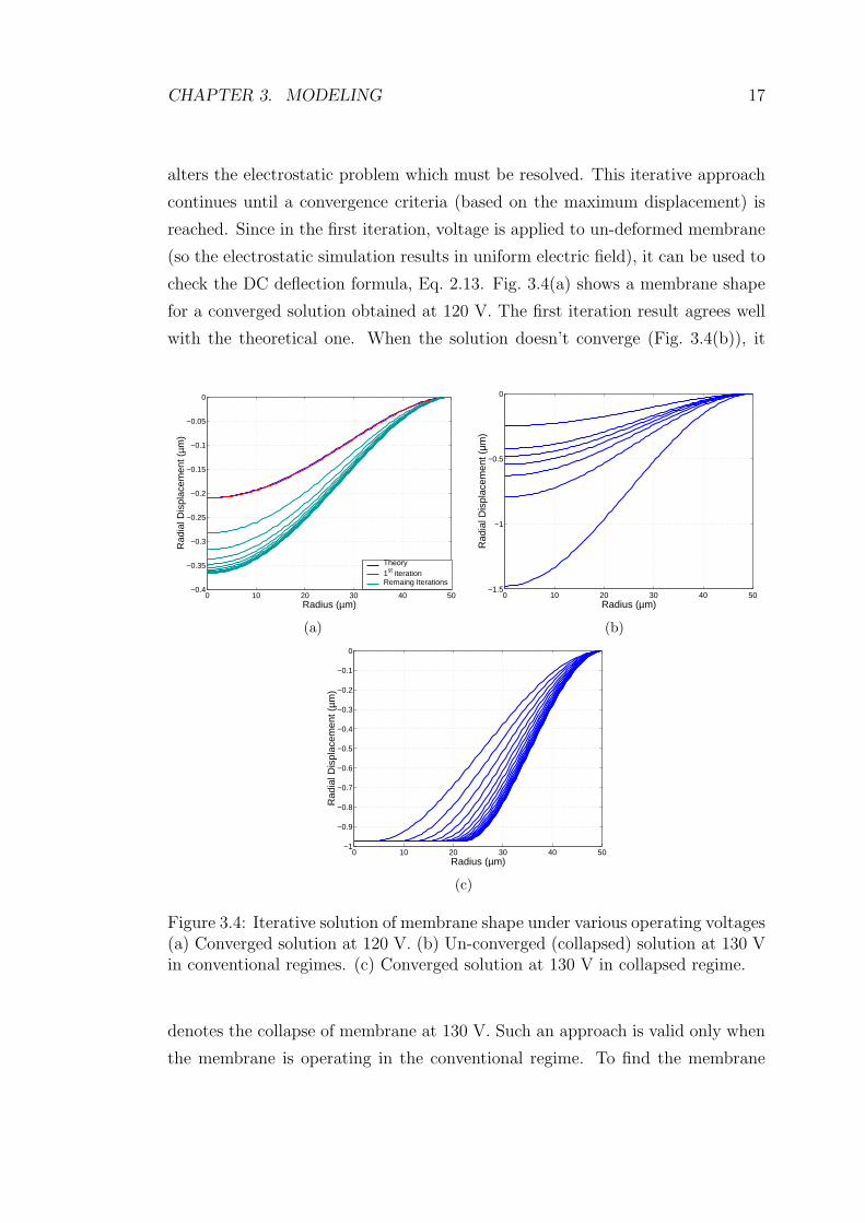
alters the electrostatic problem which must be resolved. This iterative approach
continues until a convergence criteria (based on the maximum displacement) is
reached. Since in the first iteration, voltage is applied to un-deformed membrane
(so the electrostatic simulation results in uniform electric field), it can be used to
check the DC deflection formula, Eq. 2.13. Fig. 3.4(a) shows a membrane shape
for a converged solution obtained at 120 V. The first iteration result agrees well
with the theoretical one. When the solution doesn’t converge (Fig. 3.4(b)), it
0 10 20 30 40 50−0.4
−0.35
−0.3
−0.25
−0.2
−0.15
−0.1
−0.05
0
Radius (µm)
Rad
ial D
ispl
acem
ent (
µm)
Theory1st iterationRemaing Iterations
(a)
0 10 20 30 40 50−1.5
−1
−0.5
0
Radius (µm)
Rad
ial D
ispl
acem
ent (
µm)
(b)
0 10 20 30 40 50−1
−0.9
−0.8
−0.7
−0.6
−0.5
−0.4
−0.3
−0.2
−0.1
0
Radius (µm)
Rad
ial D
ispl
acem
ent (
µm)
(c)
Figure 3.4: Iterative solution of membrane shape under various operating voltages(a) Converged solution at 120 V. (b) Un-converged (collapsed) solution at 130 Vin conventional regimes. (c) Converged solution at 130 V in collapsed regime.
denotes the collapse of membrane at 130 V. Such an approach is valid only when
the membrane is operating in the conventional regime. To find the membrane
CHAPTER 3. MODELING 18
shape when it collapses, a preliminary simulation as described above to find Vcol
must be performed. Then, the center of the un-deformed membrane is displaced
an amount of %95 of gap height (such an offset is required for meshing ease)
and the resulting structural problem is solved which gives the new finite element
model. The remaining steps are the same as the previously described approach.
An energy based convergence criteria is used. Fig. 3.4(c) shows the resulting
membrane shape for collapsed membrane at 130 V.
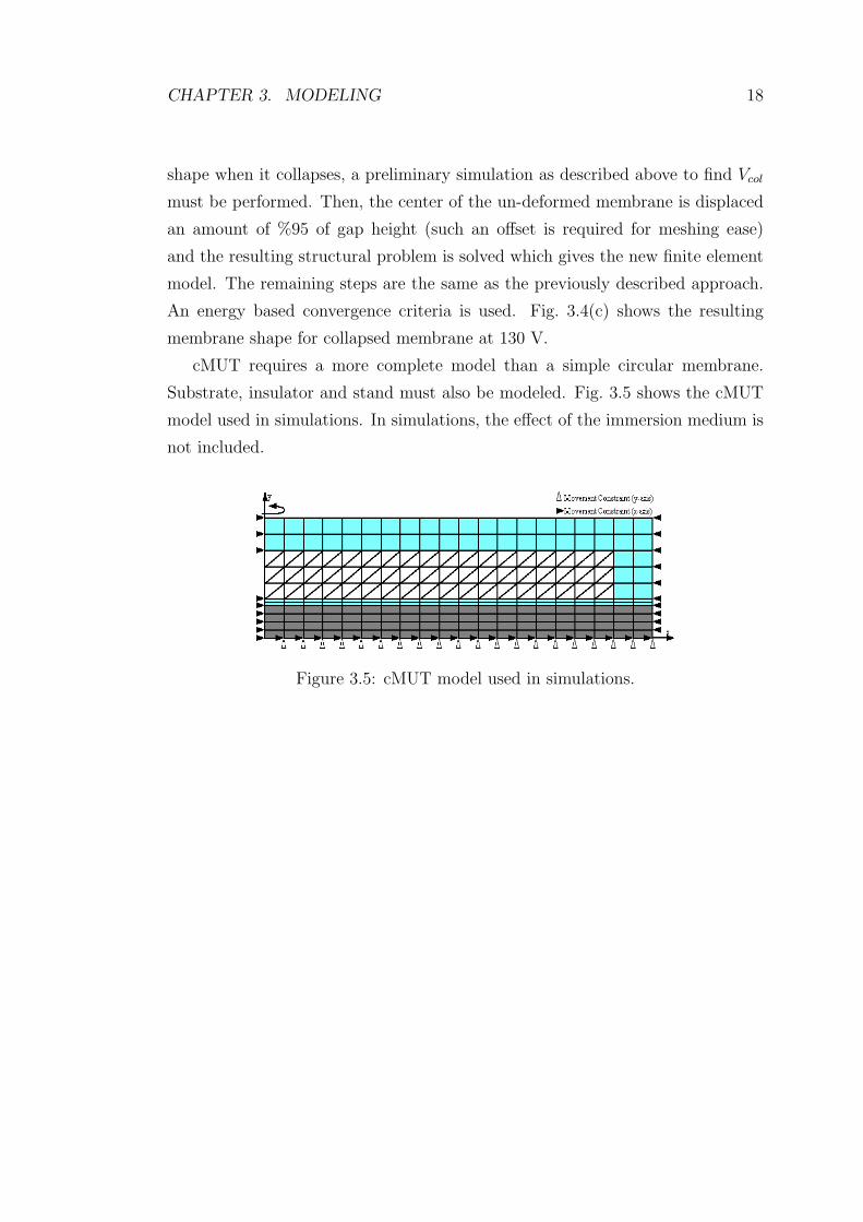
cMUT requires a more complete model than a simple circular membrane.
Substrate, insulator and stand must also be modeled. Fig. 3.5 shows the cMUT
model used in simulations. In simulations, the effect of the immersion medium is
not included.
Figure 3.5: cMUT model used in simulations.
Chapter 4
RESULTS AND DISCUSSIONS
In this chapter, cMUTs having uniform and nonuniform membranes are com-
pared using the performance measures defined in [7] for both receive and transmit
modes when cMUT is immersed in water. Those performance measures are ad-
vantageous, since they enable monitoring both the gain and the bandwidth of the
transducer. The tradeoff between these two is shown by changing various param-
eters of the device, namely the gap height (tg), and axial membrane dimensions
(a, a1 and a2), (tm, tm1 and tm2) and the termination at the electrical side (RS).
Each of these parameters are optimized for different membrane configurations
and operation modes.
The chapter begins with the investigation of effect of the electrode size on the
shunt input capacitance (C0), turns ratio (n) and collapse voltage (Vcol) of the
device. A suitable pattern is proposed for both of the membrane types, without
changing n and Vcol, but with a reduced C0. To make a fair comparison between
the performance of the devices later in the chapter, the natural resonance fre-
quencies, fr, of the membranes are held constant, hence the chapter continues
with the results showing the change of fr and the antiresonance frequency, fa, of
the membranes with respect to different membrane dimensions. The remaining
of the chapter is devoted to the definitions of figure of merits for both receive,
MR, and transmit, MT , modes and the comparison of the membranes. Each of
the results are obtained by conducting finite element (FE) simulations.
19
CHAPTER 4. RESULTS AND DISCUSSIONS 20
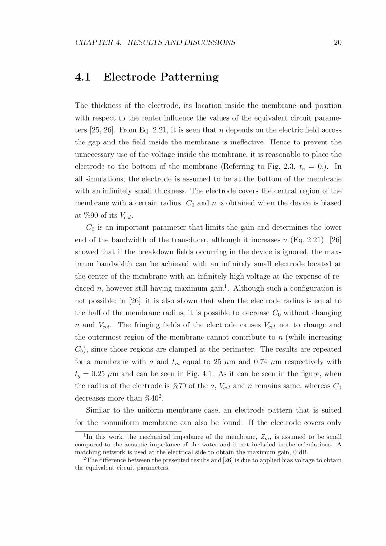
4.1 Electrode Patterning
The thickness of the electrode, its location inside the membrane and position
with respect to the center influence the values of the equivalent circuit parame-
ters [25, 26]. From Eq. 2.21, it is seen that n depends on the electric field across
the gap and the field inside the membrane is ineffective. Hence to prevent the
unnecessary use of the voltage inside the membrane, it is reasonable to place the
electrode to the bottom of the membrane (Referring to Fig. 2.3, te = 0.). In
all simulations, the electrode is assumed to be at the bottom of the membrane
with an infinitely small thickness. The electrode covers the central region of the
membrane with a certain radius. C0 and n is obtained when the device is biased
at %90 of its Vcol.
C0 is an important parameter that limits the gain and determines the lower
end of the bandwidth of the transducer, although it increases n (Eq. 2.21). [26]
showed that if the breakdown fields occurring in the device is ignored, the max-
imum bandwidth can be achieved with an infinitely small electrode located at
the center of the membrane with an infinitely high voltage at the expense of re-
duced n, however still having maximum gain1. Although such a configuration is
not possible; in [26], it is also shown that when the electrode radius is equal to
the half of the membrane radius, it is possible to decrease C0 without changing
n and Vcol. The fringing fields of the electrode causes Vcol not to change and
the outermost region of the membrane cannot contribute to n (while increasing
C0), since those regions are clamped at the perimeter. The results are repeated
for a membrane with a and tm equal to 25 µm and 0.74 µm respectively with
tg = 0.25 µm and can be seen in Fig. 4.1. As it can be seen in the figure, when
the radius of the electrode is %70 of the a, Vcol and n remains same, whereas C0
decreases more than %402.
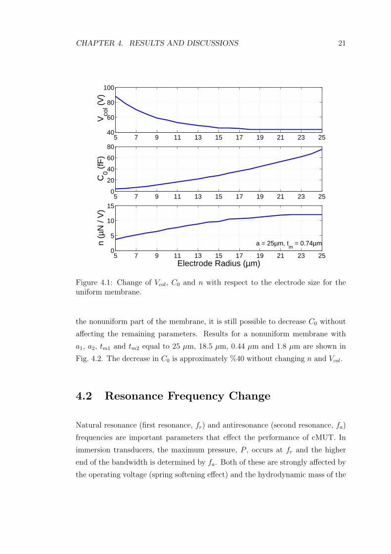
Similar to the uniform membrane case, an electrode pattern that is suited
for the nonuniform membrane can also be found. If the electrode covers only
1In this work, the mechanical impedance of the membrane, Zm, is assumed to be smallcompared to the acoustic impedance of the water and is not included in the calculations. Amatching network is used at the electrical side to obtain the maximum gain, 0 dB.
2The difference between the presented results and [26] is due to applied bias voltage to obtainthe equivalent circuit parameters.
CHAPTER 4. RESULTS AND DISCUSSIONS 21
5 7 9 11 13 15 17 19 21 23 2540
60
80
100
Vco
l (V
)
5 7 9 11 13 15 17 19 21 23 250
20
40
60
80
C0 (
fF)
5 7 9 11 13 15 17 19 21 23 250
5
10
15
n (µ
N /
V)
Electrode Radius (µm)
a = 25µm, tm
= 0.74µm
Figure 4.1: Change of Vcol, C0 and n with respect to the electrode size for theuniform membrane.
the nonuniform part of the membrane, it is still possible to decrease C0 without
affecting the remaining parameters. Results for a nonuniform membrane with
a1, a2, tm1 and tm2 equal to 25 µm, 18.5 µm, 0.44 µm and 1.8 µm are shown in
Fig. 4.2. The decrease in C0 is approximately %40 without changing n and Vcol.
4.2 Resonance Frequency Change
Natural resonance (first resonance, fr) and antiresonance (second resonance, fa)
frequencies are important parameters that effect the performance of cMUT. In
immersion transducers, the maximum pressure, P , occurs at fr and the higher
end of the bandwidth is determined by fa. Both of these are strongly affected by
the operating voltage (spring softening effect) and the hydrodynamic mass of the
CHAPTER 4. RESULTS AND DISCUSSIONS 22
5 7 9 11 13 15 17 19 21 23 2560
100
150
200
240
Vco
l (V
)
5 7 9 11 13 15 17 19 21 23 250
25
50
75
100
C0 (
fF)
5 7 9 11 13 15 17 19 21 23 255
10
15
20
25
n (µ
N /
V)
Electrode Radius (µm)
a1 = 25µm, t
m1 = 0.44µm
a2 = 18.5µm, t
m2 = 1.8µm
Figure 4.2: Change of Vcol, C0 and n with respect to the electrode size for thenonuniform membrane.
water, which brings additional imaginary load on the membrane. In this work,
hydrodynamic mass is not modeled.
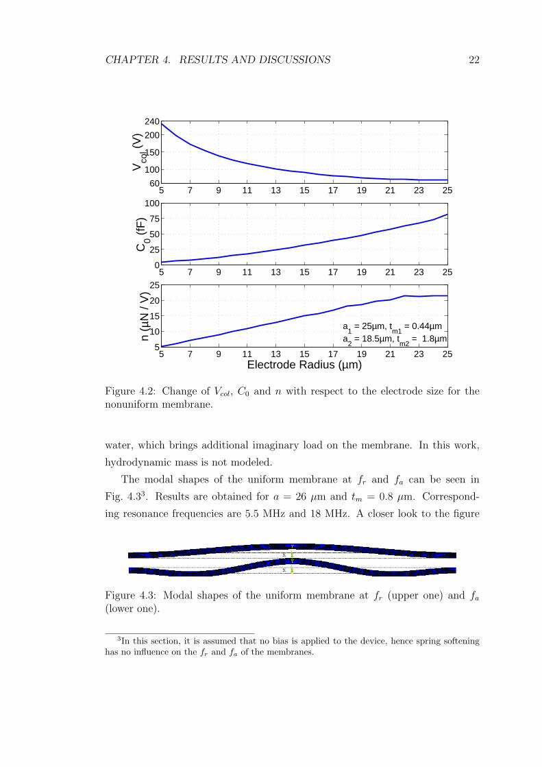
The modal shapes of the uniform membrane at fr and fa can be seen in
Fig. 4.33. Results are obtained for a = 26 µm and tm = 0.8 µm. Correspond-
ing resonance frequencies are 5.5 MHz and 18 MHz. A closer look to the figure
Figure 4.3: Modal shapes of the uniform membrane at fr (upper one) and fa
(lower one).
3In this section, it is assumed that no bias is applied to the device, hence spring softeninghas no influence on the fr and fa of the membranes.
CHAPTER 4. RESULTS AND DISCUSSIONS 23
indicates that at fr, all the points on the membrane deflect at the same direc-
tion, whereas at fa, the central region of the membrane deflects at the opposite
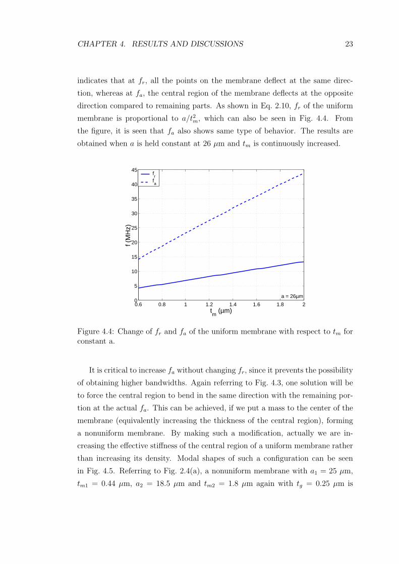
direction compared to remaining parts. As shown in Eq. 2.10, fr of the uniform
membrane is proportional to a/t2m, which can also be seen in Fig. 4.4. From
the figure, it is seen that fa also shows same type of behavior. The results are
obtained when a is held constant at 26 µm and tm is continuously increased.
0.6 0.8 1 1.2 1.4 1.6 1.8 20
5
10
15
20
25
30
35
40
45
tm
(µm)
f (M
Hz)
frfa
a = 26µm
Figure 4.4: Change of fr and fa of the uniform membrane with respect to tm forconstant a.
It is critical to increase fa without changing fr, since it prevents the possibility
of obtaining higher bandwidths. Again referring to Fig. 4.3, one solution will be
to force the central region to bend in the same direction with the remaining por-
tion at the actual fa. This can be achieved, if we put a mass to the center of the
membrane (equivalently increasing the thickness of the central region), forming
a nonuniform membrane. By making such a modification, actually we are in-
creasing the effective stiffness of the central region of a uniform membrane rather
than increasing its density. Modal shapes of such a configuration can be seen
in Fig. 4.5. Referring to Fig. 2.4(a), a nonuniform membrane with a1 = 25 µm,
tm1 = 0.44 µm, a2 = 18.5 µm and tm2 = 1.8 µm again with tg = 0.25 µm is
CHAPTER 4. RESULTS AND DISCUSSIONS 24
Figure 4.5: Modal shapes of the nonuniform membranae at fr (upper one) andfa (lower one).
simulated.
To investigate the effect of the nonuniform portion on fr and fa, we keep a1
and tm1 constant at 40 µm and 0.8 µm, respectively. Fig. 4.6(a) shows the change
of fr and Fig. 4.6(b) shows fa with respect to increasing tm2 for various a2. The
results indicate that for constant a2 as tm2 is increased, fr initially increases to
reach a maximum value, then begins to decrease. This results in that nonuniform
membrane will have the same fr for two different tm2 values (denoted as first and
second solutions). Referring to Fig. 2.5, in the first portion, the ruling effect is
5 10 15 204
5
6
7
8
9
tm2
(µm)
f r (M
Hz)
a2 = 36µm
a2 = 35µm
a2 = 34µm
A B
a1 = 40µm, t
m1 = 0.8µm
(a)
5 10 15 2015
24
33
42
51
60
tm2
(µm)
f a (M
Hz)
B
A
a2 = 36µm
a2 = 35µm
a2 = 34µm
a1 = 40µm, t
m1 = 0.8µm
(b)
Figure 4.6: Change of (a) fr and (b) fa with respect to tm2 for various a2 whena1 and tm1 are held constant at 40 µm and 0.8 µm.
the stiffness of the membrane and increasing tm2 can be considered as increasing
the spring constant, k. At the second portion, the ruling effect is the mass of
the membrane and increase in tm2 shows itself in the increase of the mass, m.
As a2 is increased, the maximum of fr also increases. On the other hand, fa
CHAPTER 4. RESULTS AND DISCUSSIONS 25
1 2 3 4 5 6 73
3.5
4
4.5
5
5.5
6
tm2
(µm)
f r (M
Hz) a
2 = 20µm
a2 = 19µm
a2 = 18µm
B’ A’
a1 = 26µm, t
m1 = 0.4µm
(a)
1 2 3 4 5 6 710
15
20
25
30
35
40
45
tm2
(µm)
f a (M
Hz)
a1 =26µm, t
m1 = 0.4µm
a2 = 20µm
a2 = 19µm
a2 = 18µm
A’
B’
(b)
Figure 4.7: Change of (a) fr and (b) fa with respect to tm2 for various a2 whena1 and tm1 are held constant at 26 µm and 0.4 µm.
continuously increases starting from around 15 MHz to 60 MHz. The points A
(first solution) and B (second solution) in Fig. 4.6(a) have the same fr, but the
later one has a fa of 60 MHz, showing the possibility of obtaining a bandwidth
more than 50 MHz. The first solution shows a behavior similar to a uniform
membrane, since tm2 value is small. On the other hand, second solution shows a
piston like behavior due to high tm2. The results are repeated for another a1 - tm1
pair, 26 µm - 0.4 µm, can be seen in Fig. 4.7(a)-(b). Different from previous the
configuration, a decrease in fa is also seen after a critical tm2 value.
4.3 Receive Mode
In the receive mode, the input acoustic power is limited since the incoming wave
is small in amplitude due to coming from another source or being reflected from
a target. Hence it is important to use as much of the available acoustic power as
possible. To obtain the best performance, the acoustic mismatch at the mechani-
cal side (Fig. 3.1(a)) should be kept minimized. Similarly, the electrical mismatch
at the electrical side should also be kept at minimum. For such a use, transducer
CHAPTER 4. RESULTS AND DISCUSSIONS 26
power gain, GT , definition is suited. It is given by [27]
GT =power delivered to the load
available power from the source=
PL
PA
=(1− |Γs|2)|1− ΓsΓin|2 |S21|2 (1− |ΓL|2)
|1− S22ΓL|2 (4.1)
with
Γin = S11 +S21S12ΓL
1− S22ΓL
(4.2)
ΓL is the reflection coefficient at the load end and the corresponding s-parameters
for cMUT is obtained from Mason’s equivalent circuit. The highest transducer
gain is obtained if the electrical side is complex conjugately matched to receiver
impedance and the acoustic side is equal to the acoustic impedance of the immer-
sion medium. The conversion gain is defined as the square root of the transducer
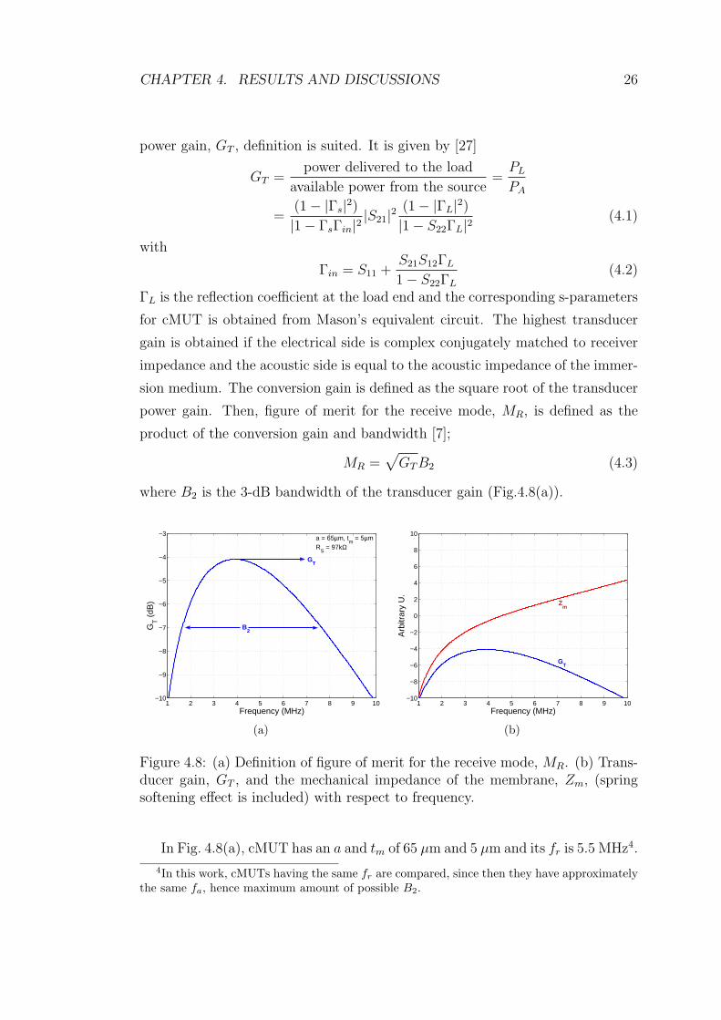
power gain. Then, figure of merit for the receive mode, MR, is defined as the
product of the conversion gain and bandwidth [7];
MR =√
GT B2 (4.3)
where B2 is the 3-dB bandwidth of the transducer gain (Fig.4.8(a)).
1 2 3 4 5 6 7 8 9 10−10
−9
−8
−7
−6
−5
−4
−3
Frequency (MHz)
GT (
dB)
B2
a = 65µm, tm
= 5µmR
S = 97kΩ
GT
(a)
1 2 3 4 5 6 7 8 9 10−10
−8
−6
−4
−2
0
2
4
6
8
10
Frequency (MHz)
Arb
itrar
y U
.
GT
Zm
(b)
Figure 4.8: (a) Definition of figure of merit for the receive mode, MR. (b) Trans-ducer gain, GT , and the mechanical impedance of the membrane, Zm, (springsoftening effect is included) with respect to frequency.
In Fig. 4.8(a), cMUT has an a and tm of 65 µm and 5 µm and its fr is 5.5 MHz4.
4In this work, cMUTs having the same fr are compared, since then they have approximatelythe same fa, hence maximum amount of possible B2.
CHAPTER 4. RESULTS AND DISCUSSIONS 27
tg is 0.25 µm and the corresponding Vcol is 118 V. 97 kΩ is used to terminate the
electrical side of single cMUT. If N cMUTs were connected in parallel, 97/N kΩ
will be required for termination5. From the small signal equivalent circuit, it is
seen that the lower end of B2, f1, is determined by the RC network formed by RS
and C0. On the other hand, f2, the high frequency end of the B2, is determined
by Zm(Fig.4.8(b)), since due to fa, Zm increases considerably resulting in the
drop of GT .
104
105
106
0
1
2
3
4
MR
(M
Hz)
104
105
1060
5
10
15
20
Termination Resistance, RS (Ω)
B2 (
MH
z)
104
105
1060
5
10
15
20
B2
MR
a = 30µm, tm
= 1.1µma = 90µm, t
m = 9.8µm
Figure 4.9: Change of MR and B2 with respect to RS for a uniform membrane.
It is clear that the termination resistance, RS, strongly affects GT and B2 by
changing the Γout at the load side. It is possible to plot GT and B2 with respect to
RS (Fig. 4.9). Two cMUTs with different radiuses, 30 µm and 90 µm, but having
the same fr are simulated. The maximum value of MR is reached at a certain RS,
showing the optimum point. However, more important than that, it is possible
to operate cMUT different from the optimum point, by changing the RS, with
a considerably high bandwidth at the expense of reduced gain. Terminating the
electrical side with 150 kΩ results in B2 of 15 MHz and MR of 3 MHz.
5In receive mode, all cMUTs are biased at %90 of their Vcol and a small AC voltage is appliedto find the equivalent circuit parameters.
CHAPTER 4. RESULTS AND DISCUSSIONS 28
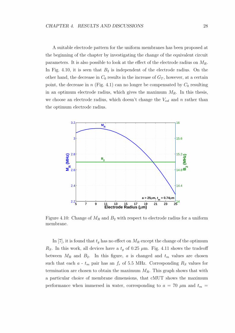
A suitable electrode pattern for the uniform membranes has been proposed at
the beginning of the chapter by investigating the change of the equivalent circuit
parameters. It is also possible to look at the effect of the electrode radius on MR.
In Fig. 4.10, it is seen that B2 is independent of the electrode radius. On the
other hand, the decrease in C0 results in the increase of GT , however, at a certain
point, the decrease in n (Fig. 4.1) can no longer be compensated by C0 resulting
in an optimum electrode radius, which gives the maximum MR. In this thesis,
we choose an electrode radius, which doesn’t change the Vcol and n rather than
the optimum electrode radius.
5 7 9 11 13 15 17 19 21 23 252.2
2.4
2.6
2.8
3
3.2
MR
(M
Hz)
5 7 9 11 13 15 17 19 21 23 2514
14.4
14.8
15.2
15.6
16
Electrode Radius (µm)
B2 (
MH
z)
MR
B2
a = 25µm, tm
= 0.74µm
Figure 4.10: Change of MR and B2 with respect to electrode radius for a uniformmembrane.
In [7], it is found that tg has no effect on MR except the change of the optimum
RS. In this work, all devices have a tg of 0.25 µm. Fig. 4.11 shows the tradeoff
between MR and B2. In this figure, a is changed and tm values are chosen
such that each a - tm pair has an fr of 5.5 MHz. Corresponding RS values for
termination are chosen to obtain the maximum MR. This graph shows that with
a particular choice of membrane dimensions, that cMUT shows the maximum
performance when immersed in water, corresponding to a = 70 µm and tm =
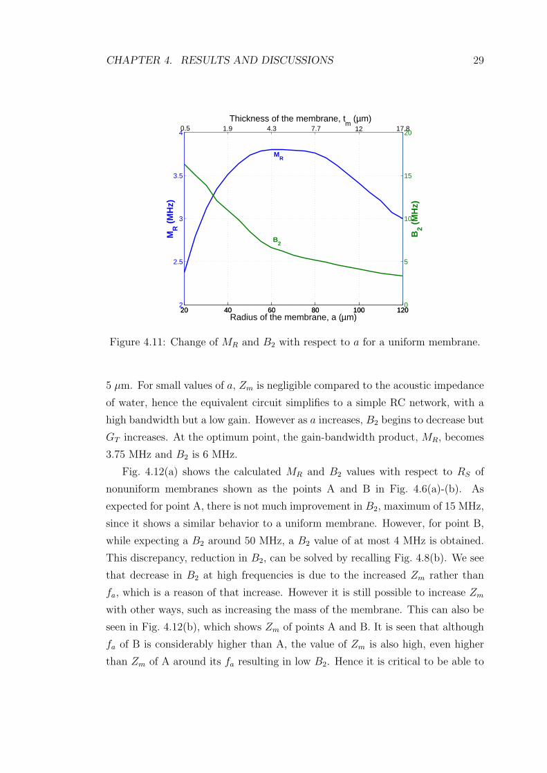
CHAPTER 4. RESULTS AND DISCUSSIONS 29
20 40 60 80 100 1202
2.5
3
3.5
4
MR
(M
Hz)
20 40 60 80 100 1200
5
10
15
20
Radius of the membrane, a (µm)
B2 (
MH
z)
B2
MR
0.5 1.9 4.3 7.7 12 17.8 Thickness of the membrane, t
m (µm)
Figure 4.11: Change of MR and B2 with respect to a for a uniform membrane.
5 µm. For small values of a, Zm is negligible compared to the acoustic impedance
of water, hence the equivalent circuit simplifies to a simple RC network, with a
high bandwidth but a low gain. However as a increases, B2 begins to decrease but
GT increases. At the optimum point, the gain-bandwidth product, MR, becomes
3.75 MHz and B2 is 6 MHz.
Fig. 4.12(a) shows the calculated MR and B2 values with respect to RS of
nonuniform membranes shown as the points A and B in Fig. 4.6(a)-(b). As
expected for point A, there is not much improvement in B2, maximum of 15 MHz,
since it shows a similar behavior to a uniform membrane. However, for point B,
while expecting a B2 around 50 MHz, a B2 value of at most 4 MHz is obtained.
This discrepancy, reduction in B2, can be solved by recalling Fig. 4.8(b). We see
that decrease in B2 at high frequencies is due to the increased Zm rather than
fa, which is a reason of that increase. However it is still possible to increase Zm
with other ways, such as increasing the mass of the membrane. This can also be
seen in Fig. 4.12(b), which shows Zm of points A and B. It is seen that although
fa of B is considerably higher than A, the value of Zm is also high, even higher
than Zm of A around its fa resulting in low B2. Hence it is critical to be able to

CHAPTER 4. RESULTS AND DISCUSSIONS 30
104
105
106
0
1
2
3
4M
R (
MH
z)
104
105
1060
4
8
12
16
Termination Resistance, RS (Ω)
B2 (
MH
z)
104
105
1060
4
8
12
16
B2
MR
a1 = 40µm, t
m1 = 0.8µm
a2 = 36µm, t
m2 = 1.8µm (A)
a2 = 36µm, t
m2 = 22µm (B)
(a)
2 3 4 5 6 7 8−0.03
−0.02
−0.01
0
0.01
0.02
Frequency (MHz)
Zm
(kg
/ s)
AB
(b)
Figure 4.12: (a) Change of MR and B2 with respect to RS for the nonuniformmembranes denoted as A and B in Fig. 4.6(a). (b) Zm of the points A and B(spring softening effect is not included).
increase fa, without increasing Zm value.
Nonuniform membrane fabricated with the sacrificial layer method is redrawn
in Fig. 4.13. To keep Zm as small as possible, one needs to keep the mass of the
membrane small and to shift fa to higher values, one needs to
• use smaller mass (smaller a2 and tm2)
• use thinner uniform region (smaller tm1)
• keep the ratio, a2/a1 small (higher a1)
Figure 4.13: Nonuniform membrane fabricated with the sacrificial layer method.
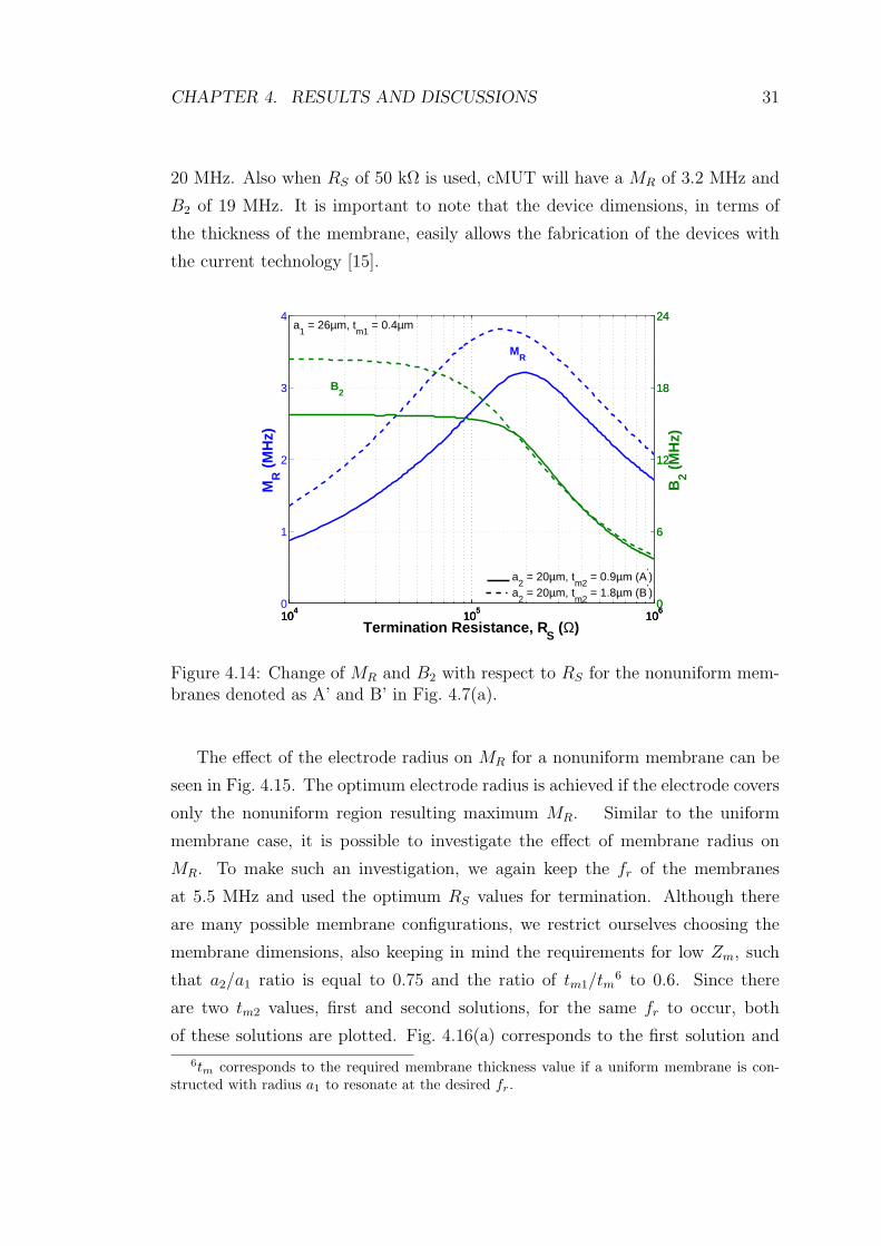
The nonuniform membranes shown as the points A’ and B’ in Fig. 4.7(a)-(b)
obeys the above considerations. The change of MR and B2 with respect to RS
can be seen in Fig. 4.14. As expected, point B’ can have a B2 of approximately
CHAPTER 4. RESULTS AND DISCUSSIONS 31
20 MHz. Also when RS of 50 kΩ is used, cMUT will have a MR of 3.2 MHz and
B2 of 19 MHz. It is important to note that the device dimensions, in terms of
the thickness of the membrane, easily allows the fabrication of the devices with
the current technology [15].
104
105
106
0
1
2
3
4
MR
(M
Hz)
104
105
1060
6
12
18
24
104
105
1060
6
12
18
24
Termination Resistance, RS (Ω)
B2 (
MH
z)
B2
MR
a1 = 26µm, t
m1 = 0.4µm
a2 = 20µm, t
m2 = 0.9µm (A’)
a2 = 20µm, t
m2 = 1.8µm (B’)
Figure 4.14: Change of MR and B2 with respect to RS for the nonuniform mem-branes denoted as A’ and B’ in Fig. 4.7(a).
The effect of the electrode radius on MR for a nonuniform membrane can be
seen in Fig. 4.15. The optimum electrode radius is achieved if the electrode covers
only the nonuniform region resulting maximum MR. Similar to the uniform
membrane case, it is possible to investigate the effect of membrane radius on
MR. To make such an investigation, we again keep the fr of the membranes
at 5.5 MHz and used the optimum RS values for termination. Although there
are many possible membrane configurations, we restrict ourselves choosing the
membrane dimensions, also keeping in mind the requirements for low Zm, such
that a2/a1 ratio is equal to 0.75 and the ratio of tm1/tm6 to 0.6. Since there
are two tm2 values, first and second solutions, for the same fr to occur, both
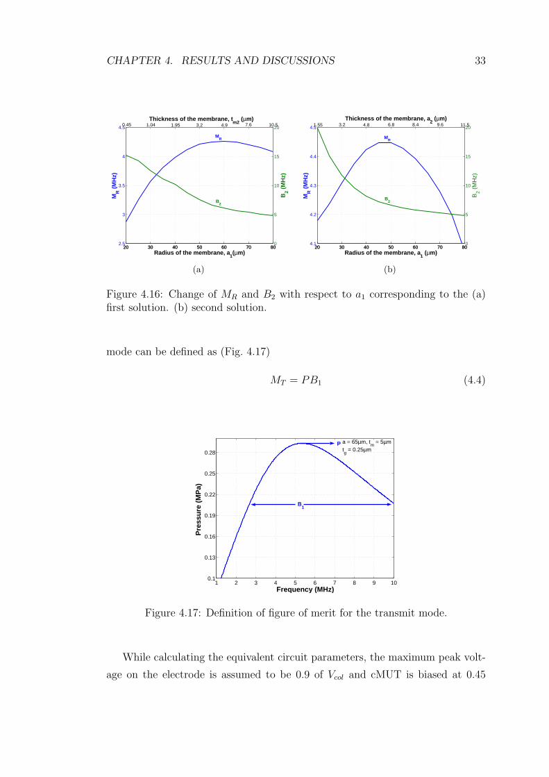
of these solutions are plotted. Fig. 4.16(a) corresponds to the first solution and
6tm corresponds to the required membrane thickness value if a uniform membrane is con-structed with radius a1 to resonate at the desired fr.

CHAPTER 4. RESULTS AND DISCUSSIONS 32
5 7 9 11 13 15 17 19 21 23 253.4
3.6
3.8
4
4.2
MR
(M
Hz)
5 7 11 13 15 17 19 21 23 2514.5
15
15.5
16
16.5
Electrode Radius (µm)
B2 (
MH
z)
a1 = 25µm, t
m1 = 0.44µm
a2 = 18.5µm, t
m2 = 1.8µm
MR
B2
Figure 4.15: Change of MR and B2 with respect to electrode radius for a nonuni-form membrane.
Fig. 4.16(b) corresponds to the second one. Since the first solution shows a similar
behavior to a uniform membrane, there is not much improvement in B2, however
with the second solution B2 can be as high as 20 MHz with a reasonably high
gain. The optimum dimension for the maximum MR is a1, tm1, a2 and tm2 are
equal to 45 µm, 1.44 µm, 33.5 µm and 4.8 µm. At that point MR is 4.45 MHz
and B2 is 7 MHz.
4.4 Transmit Mode
During the transmission mode, there is no limitation in terms of the available
power. Only limitation is the applied voltage due to the breakdown of the insu-
lator material or Vcol of the device. Referring to Fig. 3.1(b), it is important to
maximize the pressure, P , at the mechanical side, which is given by P = F/S.
Let B1 be the associated 3-dB bandwidth, then the figure of merit for the transmit
CHAPTER 4. RESULTS AND DISCUSSIONS 33
20 30 40 50 60 70 802.5
3
3.5
4
4.5
MR
(M
Hz)
20 30 40 50 60 70 800
5
10
15
20
Radius of the membrane, a1(µm)
B2 (
MH
z)
MR
B2
0.45 1.04 1.95 3.2 4.9 7.6 10.5 Thickness of the membrane, t
m2 (µm)
(a)
20 30 40 50 60 70 804.1
4.2
4.3
4.4
4.5
MR
(M
Hz)
20 30 40 50 60 70 800
5
10
15
20
Radius of the membrane, a1 (µm)
B2 (
MH
z)
MR
B2
1.55 3.2 4.8 6.8 8.4 9.6 11.5 Thickness of the membrane, a
2 (µm)
(b)
Figure 4.16: Change of MR and B2 with respect to a1 corresponding to the (a)first solution. (b) second solution.
mode can be defined as (Fig. 4.17)
MT = PB1 (4.4)
1 2 3 4 5 6 7 8 9 100.1
0.13
0.16
0.19
0.22
0.25
0.28
Frequency (MHz)
Pre
ssu
re (
MP
a)
P
B1
a = 65µm, tm
= 5µmtg = 0.25µm
Figure 4.17: Definition of figure of merit for the transmit mode.
While calculating the equivalent circuit parameters, the maximum peak volt-
age on the electrode is assumed to be 0.9 of Vcol and cMUT is biased at 0.45
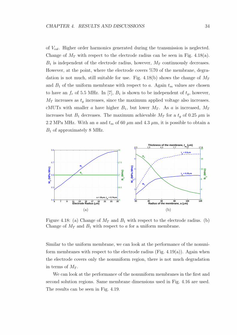
CHAPTER 4. RESULTS AND DISCUSSIONS 34
of Vcol. Higher order harmonics generated during the transmission is neglected.
Change of MT with respect to the electrode radius can be seen in Fig. 4.18(a).
B1 is independent of the electrode radius, however, MT continuously decreases.
However, at the point, where the electrode covers %70 of the membrane, degra-
dation is not much, still suitable for use. Fig. 4.18(b) shows the change of MT
and B1 of the uniform membrane with respect to a. Again tm values are chosen
to have an fr of 5.5 MHz. In [7], B1 is shown to be independent of tg, however,
MT increases as tg increases, since the maximum applied voltage also increases.
cMUTs with smaller a have higher B1, but lower MT . As a is increased, MT
increases but B1 decreases. The maximum achievable MT for a tg of 0.25 µm is
2.2 MPa MHz. With an a and tm of 60 µm and 4.3 µm, it is possible to obtain a
B1 of approximately 8 MHz.
5 7 9 11 13 15 17 19 21 23 250.4
0.5
0.6
0.7
0.8
MT (
MP
a M
Hz)
5 7 9 11 13 15 17 19 21 23 2516
16.5
17
17.5
18
Electrode Radius (µm)
B1 (
MH
z)
MT
B1
a = 25µm, tm
= 0.74µm
(a)
20 40 60 80 100 1200
1
2
3
4
5
MT (
MP
a M
Hz)
20 40 60 80 100 1200
4
8
12
16
20
Radius of the membrane, a (µm)B
1 (M
Hz)
B2
MT
tg = 0.5µm
tg = 0.25µm
0.5 1.9 4.3 7.7 12 17.8 Thickness of the membrane, t
m (µm)
(b)
Figure 4.18: (a) Change of MT and B1 with respect to the electrode radius. (b)Change of MT and B1 with respect to a for a uniform membrane.
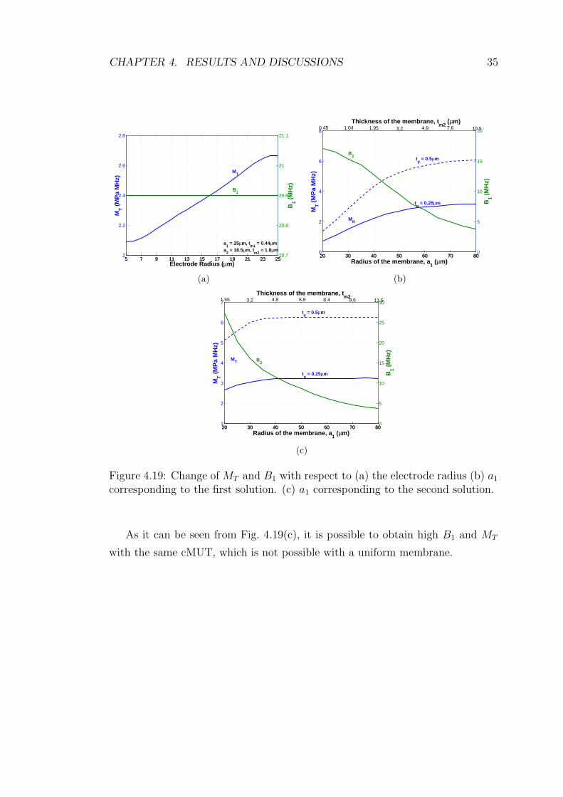
Similar to the uniform membrane, we can look at the performance of the nonuni-
form membranes with respect to the electrode radius (Fig. 4.19(a)). Again when
the electrode covers only the nonuniform region, there is not much degradation
in terms of MT .
We can look at the performance of the nonuniform membranes in the first and
second solution regions. Same membrane dimensions used in Fig. 4.16 are used.
The results can be seen in Fig. 4.19.
CHAPTER 4. RESULTS AND DISCUSSIONS 35
5 7 9 11 13 15 17 19 21 23 252
2.2
2.4
2.6
2.8
MT (
MP
a M
Hz)
5 7 9 11 13 15 17 19 21 23 2520.7
20.8
20.9
21
21.1
Electrode Radius (µm)
B1 (
MH
z)
a1 = 25µm, t
m1 = 0.44µm
a2 = 18.5µm, t
m2 = 1.8µm
MT
B1
(a)
20 30 40 50 60 70 800
2
4
6
8
MT (
MP
a M
Hz)
20 30 40 50 60 70 800
5
10
15
20
Radius of the membrane, a1 (µm)
B1 (
MH
z)
MR
B2
tg = 0.5µm
tg = 0.25µm
0.45 1.04 1.95 3.2 4.9 10.5 Thickness of the membrane, t
m2 (µm) 7.6
(b)
20 30 40 50 60 70 801
2
3
4
5
6
7
MT (
MP
a M
Hz)
20 30 40 50 60 70 800
5
10
15
20
25
30
Radius of the membrane, a1 (µm)
B1 (
MH
z)
MT B
2
tg = 0.5µm
tg = 0.25µm
1.55 3.2 4.8 6.8 8.4 9.6 11.5 Thickness of the membrane, t
m2
(c)
Figure 4.19: Change of MT and B1 with respect to (a) the electrode radius (b) a1
corresponding to the first solution. (c) a1 corresponding to the second solution.
As it can be seen from Fig. 4.19(c), it is possible to obtain high B1 and MT
with the same cMUT, which is not possible with a uniform membrane.

Chapter 5
CONCLUSION
Capacitive micromachined ultrasonic transducer (cMUT) offers high bandwidth
in low impedance media at the expense of low gain due to their low turns ratio.
A recent work [7] showed that a cMUT immersed in water can be optimized for
both high gain and bandwidth for a given frequency range.
In this work, by using the performance measures in [7], it is shown that low
gain of the cMUT is due to low turns ratio and the bandwidth of the device is lim-
ited by the antiresonance frequency of the membrane. A nonuniform membrane
is proposed to increase the turns ratio of the device and shift the antiresonance
frequency of the membrane to higher values.
First a suitable electrode pattern, which decreases the shunt input capaci-
tance, but doesn’t change the collapse voltage and turns ratio, is found. Then
the change of natural resonance and antiresonance frequencies of uniform and
nonuniform membranes for different configurations is investigated. Although
more that %200 increase in the antiresonance frequency without changing the
natural resonance frequency is obtained for a nonuniform membrane, it is also
shown that shifting the antiresonance is not enough. To obtain high bandwidth,
one also needs to decrease the membrane impedance. For a suitable nonuniform
membrane configuration, the results are obtained for both receive and transmit
modes. It is shown that without increasing the membrane impedance, it is pos-
sible to increase the antiresonance frequency %40. Various designs having high
36
CHAPTER 5. CONCLUSION 37
bandwidth and considerably high gain is presented. The membrane configura-
tions are compared for both receive and transmit modes and it is shown that use
of nonuniform membranes are advantageous in many aspects.
Future work must include the analytic modeling of the nonuniform mem-
branes, since it may be time consuming to perform finite element simulations for
each configurations for different operation modes to obtain an optimum design.
A good starting point will be the first order electromechanical model (Fig. 2.5)
introduced in chapter 2.
Appendix A
A.1 Solution Of Mason’s Differential Equation
The equation,
(Y0 + T )t3m12(1− σ2)
∇4y(r)− tmT∇2y(r)− P − ω2tmρy(r) = 0 (A.1)
is known to have a solution of the form
y(r) = AJ0(k1r) + BJ0(k2r) + CY0(k1r) + DY0(k2r)− P
ω2tmρ(A.2)
where J0() is the zeroth order Bessel function of the first kind and Y0() is the
zeroth order Bessel function of the second kind with arbitrary constants A, B,
C and D. Since r = 0 is the singular point of Y0() which leads to physically
unrealistic solution; we deduce that C = D = 0.
In polar coordinates using symmetry (no variation on φ); the Laplacian oper-
ator is equal to,
∇2y(r) =d2y(r)
dr2+
1
r
dy(r)
dr(A.3)
and for x(r) = AJ0(kr), we obtain
∇2y(r) = ∇2(AJ0(kr)) = −Ak2J0(kr) (A.4)
Similarly the Bilaplacian operator is,
∇4y(r) =d4y(r)
dr4+
2
r
d3y(r)
dr3− 1
r2
d2y(r)
dr2+
1
r3
dy(r)
dr(A.5)
38
APPENDIX A. 39
and for x(r) = AJ0(kr),
∇4y(r) = ∇4(AJ0(kr)) = Ak4J0(kr) (A.6)
If we plug (A.2) in (A.1); we obtain the characteristic equation,
(Y0 + T )t2m12(1− σ2)ρ
k41,2 +
T
ρk2
1,2 − ω2 = 0 (A.7)
Following Mason’s notation; define
c =(Y0 + T )t2m12(1− σ2)ρ
, d =T
ρ(A.8)
then the solution to A.7 is,
k1,2(1) =
√−d +
√d2 + 4cω2
2cand k1,2(2) = −
√−d +
√d2 + 4cω2
2c
k1,2(3) =j
√d +
√d2 + 4cω2
2cand k1,2(4) = −j
√d +
√d2 + 4cω2
2c(A.9)
Since J0(−x) = J0(x); let’s choose the roots with the positive signs.
We need two boundary conditions to determine A and B, which are
y(r)|r=a = 0 =⇒ AJ0(k1a) + BJ0(k2a) =P
ω2ltρ
dy(r)
dr
r=a
= 0 =⇒ Ak1J1(k1a) + Bk2J1(k2a) = 0 (A.10)
After the determination of the constants, y(r) is given by
y(r) =P
ω2tmρ
[−k2J1(k2a)J0(k1r) + k1J1(k1a)J0(k2r)
−k2J1(k2a)J0(k1a) + k1J1(k1a)J0(k2a)− 1
](A.11)
The velocity of the membrane is v(r) = jωy(r); then the average velocity, v,
is the integration of this velocity over whole membrane divided by area, S = πa2,
which is
v =1
πa2
∫ 2π
0
∫ a
0
v(r)rdrdθ =jω
πa2
∫ 2π
0
∫ a
0
y(r)rdrdθ (A.12)
using the identity∫
xJ0(αx)dx = 1αxJ1(αx); we obtain
v =jP2
a2ωltρ
[ −k2J1(k2a)J1(k1r)r
(−k2J1(k2a)J0(k1a) + k1J1(k1a)J0(k2a))k1
+
k1J1(k1a)J1(k2r)r
(−k2J1(k2a)J0(k1a) + k1J1(k1a)J0(k2a))k2
− r2
2
]
a
0
(A.13)
APPENDIX A. 40
Finally, the average velocity is given by
v =jP
ωltρ
[ 2(k21 − k2
2)J1(k1a)J1(k2a)
ak1k2(−k2J1(k2a)J0(k1a) + k1J1(k1a)J0(k2a))− 1
](A.14)
And by definition, the mechanical impedance is given by the uniform pressure,
P , applied to the membrane divided by average velocity, v. Hence Zm is
Zm =P
v
= jωltρ[ ak1k2(−k2J1(k2a)J0(k1a) + k1J1(k1a)J0(k2a))
ak1k2(−k2J1(k2a)J0(k1a) + k1J1(k1a)J0(k2a))− 2(k21 − k2
2)J1(k1a)J1(k2a)
]
(A.15)
A.2 Derivation Of Operation Parameters
The capacitance between the electrodes is the series combination of three capaci-
tances; namely membrane, gap and insulator (Fig. 2.3). These three capacitances
can be written in the differential form as
dCm =εm
teds , dCg =
ε0
tg − y(r)ds and dCi =
εi
tids (A.16)
Series combination of these differential capacitances is given by
dC0 =dCmdCgdCi
dCmdCg + dCmdCi + dCgdCi
=ε0εrmεri
εrmti + εrmεri(tg − y(r)) + εriteds (A.17)
The total capacitance is equal to the integration of the differential capacitance
over whole area, which is
C0 =
∫ 2π
0
∫ a+teff
0
ε0εrmεri
εrmti + εrmεri(tg − y(r)) + εriterdrdθ
' S ′ε0εrmεri
εrmti + εrmεritg0 + εrite(A.18)
where S ′ is the area of the membrane with extended radius to include the fring-
ing fields. Approximation is performed under the assumption that all points of
membrane deflected at the same amount, which is tg − tg0.
APPENDIX A. 41
Second step is to derive the turns ratio, n. Again referring to Fig. 2.3, total
current, I, flowing through cMUT under operation is given by
I =dQ
dt=
d
dt
(C(t)V (t)
)= C(t)
dV (t)
dt+ V (t)
dC(t)
dt(A.19)
where V (t) is the total applied voltage and C(t) is the time variable capacitance.
Under the small signal approximation; we can separate the static and dynamic
parts of V (t) and C(t) as; V (t) = VDC +VAC sin(ωt) and C(t) = C0+CAC sin(ωt+
φ) with VAC ¿ VDC and CAC ¿ C0. Then (A.19) can be approximated as
I ≈ C0dVAC(t)
dt+ VDC
dCAC(t)
dt(A.20)
When the time derivative for CAC is calculated
I ≈ C0dVAC(t)
dt− VDC
Sε0(εrmεri)2
(εrmti + εrmεritg0 + εrite)2
︸ ︷︷ ︸n
dtg(t)
dt︸ ︷︷ ︸v
≈ C0dVAC(t)
dt− nv (A.21)
where dtg(t)/dt is the average velocity of the membrane. (A.21) shows the con-
version of a mechanical quantity, v, to an electrical quantity, I. Then n is
n =S ′ε0(εrmεri)
2
(εrmti + εrmεritg0 + εrite)2VDC (A.22)
Last step is to find Vcol. First order model shown in Fig. 2.5 is suited for
calculation. The accelerating force exerted by the mass is Fmass = my(r, t) and
the restoring force of the spring is Fspring = −ky(r, t). The electrostatic force
exerted by the capacitor under constant voltage assumption is
FE =dWe
dy(r, t)=
d
dy(r, t)
(1
2CV 2
)=
V 2
2
dC
dy(r, t)
=− 1
2
Sε0(εrmεri)2
(εrmti + εrmεri(tg − y(r, t)) + εrite)2V 2 (A.23)
The sum of these three forces will be 0 at the equilibrium, hence
FN =Fmass − FE − Fspring
m∂2y(r, t)
∂t2− 1
2
Sε0(εrmεri)2
(εrmti + εrmεri(tg − y(r, t)) + εrite)2V 2 + ky(r, t) = 0
(A.24)
APPENDIX A. 42
Since DC behavior is considered, time derivative term can be set to 0; to obtain
(time and spatial dependence have been left out)
FN = ky − 1
2
Sε0(εrmεri)2
(εrmti + εrmεri(tg − y) + εrite)2= 0 (A.25)
The membrane collapses when the derivative of FN is set to 0 showing the unstable
behavior of membrane. The inflection displacement is
y(r)|r=0 =teff
3(A.26)
where the effective gap height, teff is
teff = tg +εrmti + εrite
εrmεri
(A.27)
and at that point collapse voltage, Vcol, is
Vcol =
√128Y0t3mt3eff
36ε0(1− σ2)a4(A.28)
Appendix B
Finite Element Simulation
ANSYSTM 8.1, a commercially available finite element package, is used in simula-
tions. The simulations are composed of two parts. The first part, static analysis,
yields the deflected membrane shape, shunt input capacitance (CO) and DC elec-
tric fields used in the second step for an applied DC voltage. The second part,
dynamic analysis, yields the mechanical impedance of the membrane (Zm) and
turns ratio (n).
Structural and electrostatic regions are modeled with PLANE82 and
PLANE121 elements [28]. An infinitely small thickness metal electrode is as-
sumed instead of putting a full thickness metal electrode, which doesn’t effect the
results considerably [25]. TARGE169-CONTA172 element pair is used for the
contact region that forms between the membrane and insulator when membrane
collapses. The model is meshed with quadrilateral elements except the gap, which
is meshed with triangles for re-meshing ease. For all elements, axis-symmetric op-
tion is enabled which denotes 3600 rotation around the symmetry axis that passes
through the center. Hence only the cross-section of the structure is modeled.
43

APPENDIX B. FINITE ELEMENT SIMULATION 44
(a)
(b)
Figure B.1: Application of (a) voltages and (b) electrostatic forces to FEM
B.1 Static Analysis
When a voltage is applied to the membrane, resulting electrostatic fields hence
the forces can be solved. When those forces are applied to the membrane, it
will deflect towards the insulator. However such a deflection will call a change in
electrostatic fields and forces. So the electrostatic problem must be resolved for
this new configuration, which must be followed by another structural analysis [29].
This iterative process will continue until a convergence criterion depending on
the choice is reached. The following part summarizes the steps for the solution
of membrane operating in the conventional regime.
• VDC is applied to each node on the electrode (Fig. B.1(a)).
• Resulting electric field due to the voltage distribution is solved. (Electro-
static problem)
• The electric field underneath the electrode is squared and multiplied with
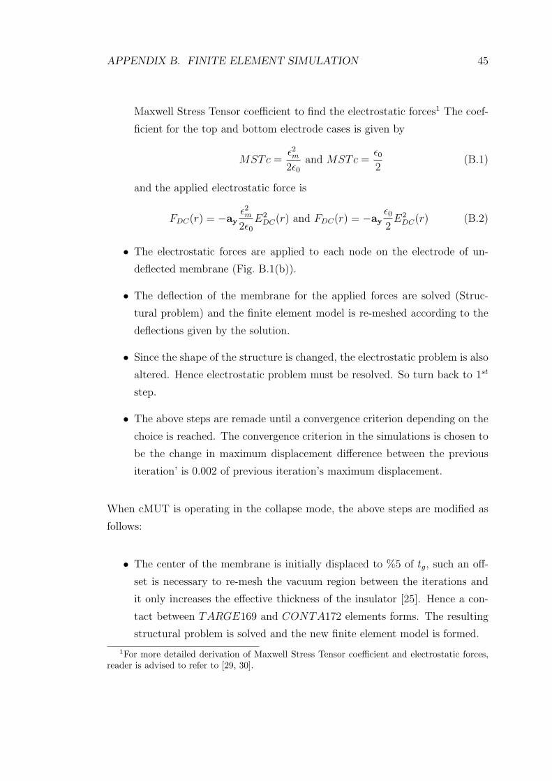
APPENDIX B. FINITE ELEMENT SIMULATION 45
Maxwell Stress Tensor coefficient to find the electrostatic forces1 The coef-
ficient for the top and bottom electrode cases is given by
MSTc =ε2m
2ε0
and MSTc =ε0
2(B.1)
and the applied electrostatic force is
FDC(r) = −ayε2m
2ε0
E2DC(r) and FDC(r) = −ay
ε0
2E2
DC(r) (B.2)
• The electrostatic forces are applied to each node on the electrode of un-
deflected membrane (Fig. B.1(b)).
• The deflection of the membrane for the applied forces are solved (Struc-
tural problem) and the finite element model is re-meshed according to the
deflections given by the solution.
• Since the shape of the structure is changed, the electrostatic problem is also
altered. Hence electrostatic problem must be resolved. So turn back to 1st
step.
• The above steps are remade until a convergence criterion depending on the
choice is reached. The convergence criterion in the simulations is chosen to
be the change in maximum displacement difference between the previous
iteration’ is 0.002 of previous iteration’s maximum displacement.
When cMUT is operating in the collapse mode, the above steps are modified as
follows:
• The center of the membrane is initially displaced to %5 of tg, such an off-
set is necessary to re-mesh the vacuum region between the iterations and
it only increases the effective thickness of the insulator [25]. Hence a con-
tact between TARGE169 and CONTA172 elements forms. The resulting
structural problem is solved and the new finite element model is formed.
1For more detailed derivation of Maxwell Stress Tensor coefficient and electrostatic forces,reader is advised to refer to [29, 30].
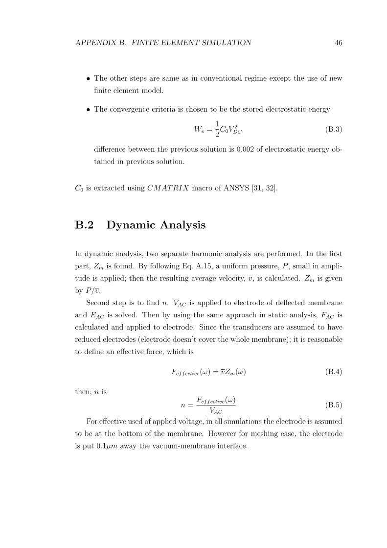
APPENDIX B. FINITE ELEMENT SIMULATION 46
• The other steps are same as in conventional regime except the use of new
finite element model.
• The convergence criteria is chosen to be the stored electrostatic energy
We =1
2C0V
2DC (B.3)
difference between the previous solution is 0.002 of electrostatic energy ob-
tained in previous solution.
C0 is extracted using CMATRIX macro of ANSYS [31, 32].
B.2 Dynamic Analysis
In dynamic analysis, two separate harmonic analysis are performed. In the first
part, Zm is found. By following Eq. A.15, a uniform pressure, P , small in ampli-
tude is applied; then the resulting average velocity, v, is calculated. Zm is given
by P/v.
Second step is to find n. VAC is applied to electrode of deflected membrane
and EAC is solved. Then by using the same approach in static analysis, FAC is
calculated and applied to electrode. Since the transducers are assumed to have
reduced electrodes (electrode doesn’t cover the whole membrane); it is reasonable
to define an effective force, which is
Feffective(ω) = vZm(ω) (B.4)
then; n is
n =Feffective(ω)
VAC
(B.5)
For effective used of applied voltage, in all simulations the electrode is assumed
to be at the bottom of the membrane. However for meshing ease, the electrode
is put 0.1µm away the vacuum-membrane interface.
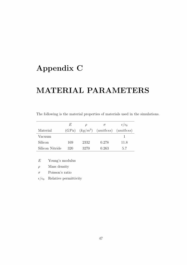
Appendix C
MATERIAL PARAMETERS
The following is the material properties of materials used in the simulations.
E ρ σ ε/ε0
Material (GPa) (kg/m3) (unitless) (unitless)
Vacuum 1
Silicon 169 2332 0.278 11.8
Silicon Nitride 320 3270 0.263 5.7
E Young’s modulus
ρ Mass density
σ Poisson’s ratio
ε/ε0 Relative permittivity
47
Bibliography
[1] B. Bayram, E. Hæggstrom, G. G. Yaralioglu, and B. T. Khuri-Yakub, “A
new regime for operating capacitive micromachined ultrasonic transducers,”
IEEE Transactions on Ultrasonics, Ferroelectrics, and Frequency Control,
vol. 50, no. 9, pp. 1184 – 1190, 2003.
[2] D. Ensminger, Ultrasonics. New York: Marcel Dekker, Inc., 1988.
[3] J. D. N. Cheeke, Fundamentals and Applications of Ultrasonic Waves.
Florida: CRC Press, 2002.
[4] G. S. Kino, Acoustic Waves: Devices, Imaging, and Analog Signal Process-
ing. New Jersey: Prentice-Hall, Inc., 1987.
[5] http://www.morganelectroceramics.com.
[6] M. I. Haller and B. T. Khuri-Yakub, “A surface micromachined electrostatic
ultrasonic air transducer,” in IEEE Ultrasonics Symposium, 1994.
[7] S. Olcum, M. N. Senlik, and A. Atalar, “Optimization of the gain-bandwidth
product of capacitive micromachined ultrasonic transducer,” IEEE Transac-
tions on Ultrasonics, Ferroelectrics, and Frequency Control, to be published.
[8] I. Ladabaum, X. Jin, H. T. Soh, A. Atalar, and B. T. Khuri-Yakub, “Surface
micromachined capacitive ultrasonic transducers,” IEEE Transactions on
Ultrasonics, Ferroelectrics, and Frequency Control, vol. 45, no. 3, pp. 1364 –
1374, 1998.
48

BIBLIOGRAPHY 49
[9] O. Oralkan, A. S. Ergun, J. A. Johnson, M. Karaman, U. Demirci, K. Ka-
viani, T. H. Lee, and B. T. Khuri-Yakub, “Capacitive micromachined ul-
trasonic transducers: Next-generation arrays for acoustic imaging,” IEEE
Transactions on Ultrasonics, Ferroelectrics, and Frequency Control, vol. 49,
no. 11, pp. 1596 – 1610, 2002.
[10] O. Oralkan, A. S. Ergun, C. H. Cheng, J. A. Johnson, M. Karaman, T. H.
Lee, and B. T. Khuri-Yakub, “Volumetric ultrasound imaging using 2-d cmut
arrays,” IEEE Transactions on Ultrasonics, Ferroelectrics, and Frequency
Control, vol. 50, no. 11, pp. 1581 – 1594, 2003.
[11] G. G. Yaralioglu, A. S. Ergun, B. Bayram, E. Hæggstrom, and B. T. Khuri-
Yakub, “Calculation and measurement of electromechanical coupling coef-
ficient of capacitive micromachined ultrasonic transducers,” IEEE Transac-
tions on Ultrasonics, Ferroelectrics, and Frequency Control, vol. 50, no. 4,
pp. 449 – 456, 2003.
[12] X. Jin, O. Oralkan, F. L. Degertekin, and B. T. Khuri-Yakub, “Fabrication
and characterization of surface micromachined ultrasonic immersion trans-
ducer,” IEEE Transactions on Ultrasonics, Ferroelectrics, and Frequency
Control, vol. 48, no. 3, pp. 750 – 760, 2001.
[13] X. Jin, I. Ladabaum, and B. T. Khuri-Yakub, “The microfabrication of ca-
pacitive ultrasonic transducers,” Journal of Micromechanical Systems, vol. 7,
no. 3, pp. 295 – 302, 1998.
[14] X. Jin, I. Ladabaum, , F. L. Degertekin, S. Calmes, and B. T. Khuri-
Yakub, “Fabrication and characterization of surface micromachined ultra-
sonic immersion transducer,” IEEE Journal of Microelectromechanical Sys-
tems, vol. 8, no. 1, pp. 100 – 114, 1999.
[15] Y. Huang, A. S. Ergun, Edward, M. H. Badi, and B. T. Khuri-Yakub, “Fabri-
cating capacitive micromachined ultrasonic transducers with wafer-bonding
technology,” Journal of Micromechanical Systems, vol. 12, no. 2, pp. 128 –
137, 2003.

BIBLIOGRAPHY 50
[16] B. Bayram, E. Hæggstrom, A. S. Ergun, G. G. Yaralioglu, and B. T. Khuri-
Yakub, “Dynamic analysis of cmuts in different regimes of operation,” in
IEEE Ultrasonics Symposium, 2003.
[17] W. P. Mason, Electromechanical Transducers and Wave Filters, 2nd ed. New
York: D. Van Nostrand Company, Inc., 1948.
[18] M. H. Badi, “Capacitive micromachined ultrasonic lamb wave transducers,”
Ph.D. dissertation, Stanford University, 2004.
[19] M. Rossi, Acoustics And Electroacoustics. Norwood, MA: Artech House,
1988.
[20] G. T. A. Kovacs, Micromachined Transducers Sourcebook. New York:
McGraw-Hill Book Company, Inc., 1998.
[21] H. A. C. Tilmans, “Equivalent circuit representation of electromechanical
transducers: I. lumped-parameter systems,” Journal of Micromechanics and
Microengineering, vol. 6, pp. 157 – 176, 1996.
[22] G. G. Yaralioglu, M. H. Badi, A. S. Ergun, and B. T. Khuri-Yakub, “Im-
proved equivalent circuit and finite element method modeling of capaci-
tive micromachined ultrasonic transducer,” in IEEE Ultrasonics Symposium,
2003.
[23] A. Lohfink, P.-C. Eccardt, W. Benecke, and H. Meixner, “Derivation of a
1d cmut model from fem results for linear and nonlinear equivalent circuit
simulation,” in IEEE Ultrasonics Symposium, 2003.
[24] F. Wen, W. Li, Q. Huang, and H. Rong, “Large-signal lumped-parameter
macromodels for the equivalent circuit representation of electromechanical
transducers,” Journal of Micromechanics and Microengineering, vol. 14, pp.
452 – 461, 2004.
[25] B. Bayram, G. G. Yaralioglu, A. S. Ergun, and B. T. Khuri-Yakub, “Influ-
ence of the electrode size and location on the performance of a cmut,” in
IEEE Ultrasonics Symposium, 2001.
BIBLIOGRAPHY 51
[26] A. Bozkurt, I. Ladabaum, A. Atalar, and B. T. Khuri-Yakub, “Theory and
analysis of electrode size optimization for capacitive microfabricated ultra-
sonic transducers,” IEEE Transactions on Ultrasonics, Ferroelectrics, and
Frequency Control, vol. 46, no. 6, pp. 1364 – 1374, 1999.
[27] R. Ludwig and P. Bretchko, RF Circuit Design: Theory and Applications.
New Jersey: Prentice-Hall, Inc., 2000.
[28] ANSYS Element Reference, ANSYS User Manual, 2004.
[29] A. Bozkurt, “Modeling and characterization of capacitive micromachined
ultrasonic transducers,” Ph.D. dissertation, Bilkent University, 2000.
[30] R. Plonsey and R. E. Collin, Principles and Applications of Electromagnetic
Fields. New York: McGraw-Hill Book Company, Inc., 1961.
[31] ANSYS Command Reference, ANSYS User Manual, 2004.
[32] ANSYS Theory Reference, ANSYS User Manual, 2004.


![[105]-Design and Performance Analysis of Capacitive Micromachined Ultrasonic Transducer Linear Array](https://img.dokumen.tips/doc/110x75/56d6bddc1a28ab30168f9c62/105-design-and-performance-analysis-of-capacitive-micromachined-ultrasonic.jpg)