Triple flame: Inherent asymmetries and pentasectional

Combustion Theory and Modelling, 2014

Vol. 18, No. 3, 454–473, http://dx.doi.org/10.1080/13647830.2014.923116

Triple flame: Inherent asymmetries and pentasectional character

Albert Jorda Juanos∗ and William A. Sirignano

Department of Mechanical and Aerospace Engineering, University of California, Irvine, CA92697-3975, USA

(Received 24 February 2014; final version received 5 May 2014)

A two-dimensional triple-flame numerical model of a laminar combustion process re-flects flame asymmetric structural features that other analytical models do not generate.It reveals the pentasectional character of the triple flame, composed of the centralpure diffusion-flame branch and the fuel-rich and fuel-lean branches, each of whichis divided into two sections: a near-stoichiometric section and a previously unreportednear-flammability-limits section with combined diffusion and premixed character. Re-sults include propagation velocity, fuel and oxidiser mass fractions, temperature andreaction rates. Realistic stoichiometric ratios and reaction orders match experimentalplanar flame characteristics. Constant density, a one-step reaction, and a mixture fractiongradient at the inlet as the simulation parameter are imposed. The upstream equivalenceratio or the upstream reactant mass fractions are linear or hyperbolic functions of thetransverse coordinate. The use here of experimental kinetics data differs from previ-ous analytical works and results in flame asymmetry and different flammability limits.Upstream mixture composition gradient affects propagation velocity, flame curvature,diffusion flame reaction rate, and flammability limits. Flammability limits extend be-yond those of a planar flame due to transverse heat and mass diffusion causing thepentasectional character.

Keywords: triple flame; edge flame; diffusion flame; premixed combustion; partiallypremixed combustion

Nomenclature

A Pre-exponential factorcp Specific heat under constant pressureD Mass diffusivity

Ea Activation energy[F], [O] Fuel and Oxygen molar density

h Specific enthalpyL Domain length

Le Lewis numberm, n Reaction orders

P PressureQ Fuel heat of combustion

Ru Universal gas constantt Time

T Temperature

∗Corresponding author. Email: [email protected]

C© 2014 Taylor & Francis

Combustion Theory and Modelling 455

U Upstream velocityUo Steady-state upstream velocityW Domain width

x, y Cartesian coordinatesYF Fuel mass fractionYO Oxygen mass fraction

β1, β2 Conserved Shvab–Zel’dovich variables�t Time step

�x, �y Distance between nodes in x and yν Fuel-to-oxygen mass stoichiometric ratioρ Mixture density� Equivalence ratioω Fuel reaction rate

1. Introduction

Triple flames have been described as tri-brachial structures consisting of a fuel-rich pre-mixed flame, a fuel-lean premixed flame and a diffusion flame [1,2]. The two premixedflames form a curved flame front followed by a trailing edge that constitutes the body ofthe diffusion flame. The diffusion flame starts at the point where the two premixed flamesmeet, where the inflowing mixture is at stoichiometric proportions. Such flames, also callededge flames, appear in flows characterised by gradients of concentrations of the reactantsand they have been studied during the past decades (see Section 2).

Many combustion processes rely on the burning of gaseous reactants that initially flowseparately and subsequently form a mixing layer, generally with mixing beginning upontheir entering the combustion chamber. They react within thin reaction zones under space-and time-varying reactant concentration conditions. Such reaction zones are located at thestoichiometric surfaces and form a diffusion flame. In non-premixed turbulent conditions,such diffusion flames could be stretched and quenched locally due to velocity fluctuations,when the heat diffusing away from the reaction zone is not balanced by the heat producedby combustion. The characteristic flame structure that is observed at an edge of thestoichiometric surface bordering the extinction zone can be modelled locally by a tripleflame [3].

Thus, triple flames are physically embodied in real combustors, and it is importantto avoid undesirable combustion conditions there such as flame flashback or blow-off.Therefore, it is desirable to understand the propagation characteristics of these flames andhow to stabilise them. Furthermore, the speed of propagation of the triple flame determinessuch important properties as the flame surface increase rate in non-premixed combustionand the lift-off distance in lifted flames at burners [3].

The goal of the present numerical study is to analyse triple flames with a simplifiedmodel that describes qualitatively how the premixed branches can be split into two sections,which display the pentasectional character of the triple flame (see Figure 1). This discussionwill focus on multidimensional, steady flames where all five sections appear simultaneously.Only monotonic variation of concentration in space will be considered. The modellingperformed in the present work also addresses issues such as flame stabilisation, flammabilitylimits, temperature and shape. The background for this study will be explained in thefollowing literature review section.

456 A. Jorda Juanos and W.A. Sirignano

Figure 1. Pentasectional triple flame sketch and problem domain.

2. Literature review

Triple flames have been investigated experimentally, analytically and numerically. Theywere first observed in a buoyant methane layer experiment [4]. Other experimental studiesin which triple flames appeared include [5–12]. These studies helped to understand tripleflame properties such as propagation, stabilisation, liftoff and blowout behaviour, andconcentration and dilution effects. Collectively, they cover several flow configurations,including non-premixed jets, laminar mixing layers, two-dimensional and axisymmetriccounterflows, and liquid-film fuel combustors.

To the best knowledge of the authors, triple flames were first analysed for an unsteadypremixed flame moving through a stratified combustible mixture forming a diffusion flameas the premixed flame passed from a fuel-rich zone to a fuel-lean zone [13]. Triple flameswere also identified as transient laminar flamelets in the combustion of turbulent diffusionflames [14,15]. The analytical formulation was developed accounting for approximationssuch as small upstream concentration gradients (also called slowly-varying triple flames)[1,2], or parabolic flame paths [3]. These studies helped gain insight to Lewis numbereffects on flame structure and propagation speed decrements resulting from increments inthe upstream mixture ratio. They also revealed that the adiabatic planar flame speed is anupper boundary for the propagation speed of triple flames for the constant-density case.Another simple analytical method was used to study buoyancy effects on triple flames [16].

The articles that used numerical approaches to triple flames may be classified dependingon three important aspects: the use of constant or variable density, prescribed unity or non-unity Lewis number for the species, and one-step versus detailed chemical kinetics. Table 1shows a chronologically ordered list of articles that presented numerical results on tripleflames.

In solving problems that involve reacting flows, the choice of the model for the chemi-cal kinetics is significant. In 1981, Westbrook and Dryer [27] examined simplified reactionmechanisms for the oxidation of hydrocarbon fuels using a numerical laminar flame modelentailing one and two global reaction steps and quasi-global mechanisms. The reaction-rateparameters were changed for different combinations of hydrocarbon fuels and air, and suchparameters were adjusted to provide the best agreement between computed and experi-mentally observed planar flame speeds. The theoretical models that use 1-step chemicalreaction mechanisms entailing parameters obtained from experimental analysis have been


Table 1. Chronological classification of numerical studies.

Reference no. Density Lewis no. Chemical kinetics Laminar/Turbulent

[1] Constant Unity 1-step, unmatched parameters Laminar[17] Constant Unity 1-step, unmatched parameters Laminar[6] Constant Unity 1-step, unmatched parameters Laminar[18] Variable Non-unity 1-step, unmatched parameters Laminar[19] Variable Unity 1-step, unmatched parameters DNS[20] Constant Unity 1-step, unmatched parameters Laminar[21] Constant Variable 1-step, unmatched parameters Laminar[9] Variable Non-unity 10-step, detailed kinetics Laminar[22] Variable Non-unity C1, detailed kinetics DNS[23] Variable Non-unity 38-step, detailed kinetics DNS[16] Variable Unity 1-step, unmatched parameters Laminar[24] Variable Non-unity 38-step, detailed kinetics DNS[25] Variable Non-unity 1-step, matched parameters Laminar[26] Variable Unity 1-step, matched parameters DNS

identified in Table 1 as ‘matched’. Chemical kinetics models that are arbitrary in that sensehave been labelled ‘unmatched’.

Note that all the numerical studies listed in Table 1 that use one-step reaction mecha-nisms assume chemical kinetics with unity reaction order and identical molecular weightsfor each reactant except [25], in which the activation energy was artificially adapted as afunction of fuel-to-oxygen equivalence ratio to match real kinetic rates. A study of tripleflames entailing a one-step reaction mechanism equipped with the experimentally obtainedparameters from [27] is missing. Thus, this paper will address that need. We will assumesimplifications such as constant density and unit Lewis number, but the chemical reactionterm in the equations will be equipped with the kinetics parameters provided by [27] andthe reactants will be balanced in proper mass proportions. We will no longer maintain theartificial symmetry of many previous research works with regard to the concentration andmolecular weight of each reactant.

Although the constant-density assumption is often designated as low heat release, itdoes not mean, for example, that the amount of heat produced by the combustion processis low compared with the enthalpy of the unburned gas. The commonly used description‘low heat release’ is poor because the energy per unit mass of the combustible mixture isactually not reduced. Rather, the resulting gas expansion is ignored; so, ‘constant density’is a superior description. As opposed to the low-heat release cases in which the triple flamepropagation velocity is bounded above by the planar premixed flame speed, heat releasecauses gas expansion and redirection of the flow that produces triple flame propagationvelocities greater than the planar flame velocity. These effects depend also on the mixtureratio gradient at the inlet. The heat release causes an expansion in the gas field whichresults in the slowing of the incoming unburned gases as they approach the flame front[18]. Consequently, the free stream velocity exceeds the local flame velocity. Aside from theeffects that heat release has on flame propagation, using unity reaction orders and unmatchedchemistry parameters results in flame front shape profiles that show symmetric propertieswith respect to the stoichiometric line. Symmetry will be prevented by the kinetics that wewill use in the present study.

A review of edge-flames described tribrachial flames as ignition fronts with positivespeeds characterised by a trailing diffusion flame [28]. The solutions showed structures


which, after initial transients, propagated at well defined speeds and had unchanging shape.Under the mentioned assumptions, the present work reports results that are in agreementwith these features. However, some new features related to the pentasectional character willbe identified and discussed. The new model, numerical details and results are presented inthe following sections.

3. Model and analysis

3.1. Formulation of differential equations

The two-dimensional transient model presented is subject to the following assumptions:fluid consisting of a mixture of fuel and oxidiser (i.e. propane and air); laminar flow;uniform velocity field with x-velocity component only (U); unit Lewis number (Le = 1);constant thermal conductivity and specific heat; neglected radiative transfer; and constantdensity. The thermal conductivity and the specific heat will be evaluated for the calculationof thermal diffusivity at a mean flame temperature while the density will be assessed at theupstream conditions. The value of the heat of combustion Q is taken from the literature [29].The lower heating value is assumed throughout this study, which implies that none of thewater in the products condenses. The upstream velocity U will be adjusted conveniently inorder to stabilise the flame. Changes in U imply a change in the pressure gradient. However,the pressure time derivative term is approximated to be zero in the energy equation becausethe time change in pressure due to these small velocity adjustments will be very smallcompared to the changes in temperature through the domain. Furthermore, we are interestedin the steady-state solution reached asymptotically in time, and temporal changes duringthe transient part of the simulation are less interesting.

We define the following two Shvab-Zel’dovich variables, as well as the differentialoperator L:

β1 = YF − νYO, β2 = h + νYOQ = cpT + νYOQ (1)

L (u) = ∂u

∂t+ U

∂u

∂x− D∇2u. (2)

Under the proposed hypothesis, selected combinations of the equations of energy, fueland oxygen species yield

L (β1) = 0, L (β2) = 0, L (YF) = − ω

ρ(β1, β2, YF) . (3)

We will consider the flame to be propagating in the negative x-direction in the laboratorythrough a quiescent combustible mixture. We seek the final steady velocity of propagationUo > 0. If the reference frame moves with the flame, we have a steady free stream atvelocity Uo flowing in the positive x-direction. Then, U = Uo and the time derivative inoperator L becomes zero. However, we do not know Uo a priori, which is an eigenvalue ofthe problem.

In general, we must solve the system of equations (3). However, if we restrict the fueland oxidiser mass fractions at the inlet to be linear functions of y, we can show that thenonly a single equation has to be solved.


3.2. Initial and boundary conditions

Instead of setting initial conditions for β1 and β2, it is more intuitive to set them for the fueland oxygen mass fractions and for the temperature. Hyperbolic tangent functions of x areused to represent the decreases in fuel and oxygen mass fractions or temperature rise acrossthe flame. The initial conditions for β1 and β2 are obtained using the three previous initialconditions in Equations (1). The initial velocity value is taken from experimental data forpremixed stoichiometric planar flames.

The boundary conditions are imposed on the distributions of fuel, oxygen and tem-perature, and they prescribe the following boundary conditions for the functions β1 andβ2.

At x = L:

∂YF

∂x= 0,

∂YO

∂x= 0,

∂T

∂x= 0. (4)

At y = ±W/2:

∂2YF

∂y2= 0,

∂2YO

∂y2= 0,

∂2T

∂y2= 0. (5)

For x = 0 (inlet), the mixture ratio is a prescribed function of y and its gradient is variedand used as a parameter of the problem. In these conditions, one side of the domain becomesfuel-rich whereas the other side becomes fuel-lean. Four types of transverse variations forupstream flow are considered: linear variation of mass fraction; hyperbolic tangent variationof mass fraction; linear variation of equivalence ratio; and hyperbolic tangent variation ofequivalence ratio.

The linear variation of mass fraction allows an analytical simplification. The hyperbolictangent variation of mass fraction presents a flow similar to a mixing layer. The hyperbolictangent variation of equivalence ratio resembles profiles used previously [18]. The linearvariation of equivalence ratio provides an interesting comparison. The use of equivalenceratio is especially useful in studying flammability limits.

3.2.1. Linear mass-fraction profile

Let us now consider the particular case in which the mass fractions are linear in y farupstream (x → −∞). We also prescribe the temperature (or enthalpy) at the inlet.

YF−∞ = YFo+ k1y, YO−∞ = YOo

+ k2y, h−∞ = ho, T−∞ = To. (6)

YFoand YOo

are in stoichiometric proportions. A fuel-rich mixture exists for y < 0 and afuel-lean mixture occurs for y > 0. Then, k1 < 0 < k2.

Let us define

a = νk2 − k1 > 0, H = ho + νYOoQ, b = νk2Q > 0. (7)

Then

β1−∞ = −ay, β2−∞ = ho + νYOoQ + νk2Qy = H + by. (8)


Note that β1 = −ay and β2 = H + by become zero when differentiated once by t or x ortwice by y. Therefore, they satisfy L(β) = 0 as well as satisfying the upstream and sideboundary conditions. We have solutions to the first two equations in (3), which may besubstituted into the third one so that

L (YF) = − ω

ρ(−ay,H + by, YF) . (9)

Thus, we have shown that when the mass fractions of the reactants at the inlet are linearfunctions, only Equation (9) must be solved for YF. Since β1 and β2 are known, backsubstitution into Equations (1) will provide YO and T (which is related to the enthalpy). Thelinear profiles upstream of the flame front imply that diffusion in the y-direction is uniformand the composition will not vary along any streamline before it reaches the flame.

3.2.2. Hyperbolic tangent mass-fraction profile

In reality, it would be difficult to find purely linear functions of y at the inlet of a combustor. Inthe modelling of mixing layers, hyperbolic tangent functions are usually used to representthe velocity profile across the layer (see for example [30,31]). The hyperbolic tangentfunctions for the reactants mass fractions at the inlet are given by Equations (10):

YF−∞ = YFo[1 + tanh (k3y)] , YO−∞ = YOo

[1 + tanh (k4y)] . (10)

To be consistent with the criteria used before, we choose to have a fuel-lean mixturefor y > 0 and a fuel-rich mixture for y < 0. Then k3 < 0 and k4 > 0. In order to make thishyperbolic case comparable to the linear case, the parameters k3 and k4 are related to thelinear slopes k1 and k2 so that the maximum gradients of the hyperbolic tangent profilesmatch the slopes of the linear profiles. For any case entailing nonlinear functions at theinlet, the problem cannot be reduced to solving a single equation. Instead, the system ofequations (3) has to be solved. With this profile, diffusion fluxes in the y-direction upstreamof the flame are not uniform with y. Accordingly, some change of composition for a givenstreamline will occur upstream of the flame.

3.2.3. Linear equivalence ratio profile

For the cases in which the inflowing equivalence ratio is prescribed as a linear function weuse

�−∞ = k5y + k6. (11)

3.2.4. Hyperbolic tangent equivalence ratio profile

For the cases in which the inflowing equivalence ratio is prescribed as a hyperbolic tangentfunction we use

�−∞ = 0.5[1 + tanh(k7y)]. (12)


3.3. Chemical kinetics

Let us consider the Arrhenius one-step form for the reaction rate, where [F] and [O] are themolar density for fuel and oxygen species, respectively, and T − To is used to confront the‘cold-boundary difficulty’ [32]:

d[F]

dt= [F]m[O]nA exp

{− Ea

Ru (T − To)

}, ω = ρ

dYF

dt. (13)

For comparison purposes, two different sets of the kinetics parameters will be used:

• matched kinetics with constants from [27] (propane and air): m = 0.1, n = 1.65,Ea/Ru = 15,098 K, A = 4.84 × 109 (kmol m−3)−0.75 s−1, T0 = 300 K;

• unmatched kinetics: m = 1, n = 1.

Previous studies that used unmatched kinetics tended to provide qualitative explanationsof the flame shape and propagation rather than quantitative descriptions. Our goal here isto compare the qualitative differences between the use of matched and unmatched kinetics.To achieve this, the reaction orders are switched to unity. The original values of the oxygenmolecular weight, activation energy Ea and pre-exponential factor A are kept the same.However, the heat of combustion Q is reduced (by a factor of six) so that the propagationvelocity for stoichiometric conditions in the unmatched kinetics case equals the velocitycalculated later with the original kinetics for propane and air (0.37 m s−1). The numericalscheme specifications will be presented in the following section.

3.4. Numerical method and convergence

The domain is discretised using a Cartesian uniformly spaced two-dimensional mesh. Anexplicit forward difference is used for the transient terms, in which �t represents the stepin time, and a central difference is used for the diffusion terms. The time step is chosen sothat it satisfies the numerical stability requirements; we also use an upwind scheme for theadvection term.

After starting the code, the shape of the fuel mass fraction profile changes every step intime, from its initial profile towards a steady shape governed by Equation (3). Taking thisinto account, the upstream velocity is not changed during this initial period of simulation.Afterwards, the ‘cliff ’ of the fuel mass fraction moves forward or backward depending onhow different the upstream velocity U is compared to Uo. We adjust this velocity until the‘cliff ’ does not move. To achieve this goal, we focus on the peak value of the reaction rateand observe its change in position over time xmax (t), as shown in Figure 2. In the generalcase, the reaction rate will be a function of x and y. We will focus on the y-coordinate inwhich the peak of the reaction rate is found.

The upstream velocity is adjusted according to the following increment:

�U = xmax(t + �t) − xmax(t)

�t. (14)

Note that �U is positive when the flame moves forward. Therefore, the adjusted up-stream velocity is given by

U new = U old − �U. (15)


Figure 2. Position change of the reaction-rate peak.

After some time of repeating this iterative process during the simulation, the upstreamvelocity increment goes to 0 (�U → 0) and the upstream velocity becomes Uo. The criterionto end the simulation is the condition that �U is zero for a sufficiently long period of time(i.e. 103 × �t).

The mesh has been refined until the results have become mesh-independent, resultingin 500 nodes in each direction for a domain that is 5 mm long and 5 mm wide. Whenconsidering the minimum number of nodes to be used, we must also bear in mind that themost drastic gradients in the physical variables occur within the reaction zone. To capturethese gradients successfully with the reaction zone thickness about one-half of a millimeter,500 nodes are used in the x-direction, yielding about 50 nodes in the reaction zone. Fartherdownstream, there are about 25 nodes across the diffusion flame in the y-direction. Thesequantities are deemed to be sufficient.

In order to show that the results are independent of the size of the domain, calculationshave been performed for different domain sizes while keeping the same �x and �y as forthe 5 mm case. The results show their independence of the domain size.

4. Results and discussion

4.1. Flammability limits: Pentasectional character

One of the goals of this section is to compare the differences in flammability limits be-tween our model and the one used by Westbrook and Dryer [27] for planar flames. Theyreported equivalence ratio values for the fuel-lean and fuel-rich flammability limits of aone-dimensional planar flame of 0.5 and 3.2, respectively (for propane and air). Reduc-tion of our model to the one-dimensional case yields 0.5 and 2.8 for these two limits. So,good agreement is found for the planar case which corresponds to the experimental values.However, the theory now predicts different values for the two-dimensional case, a finding


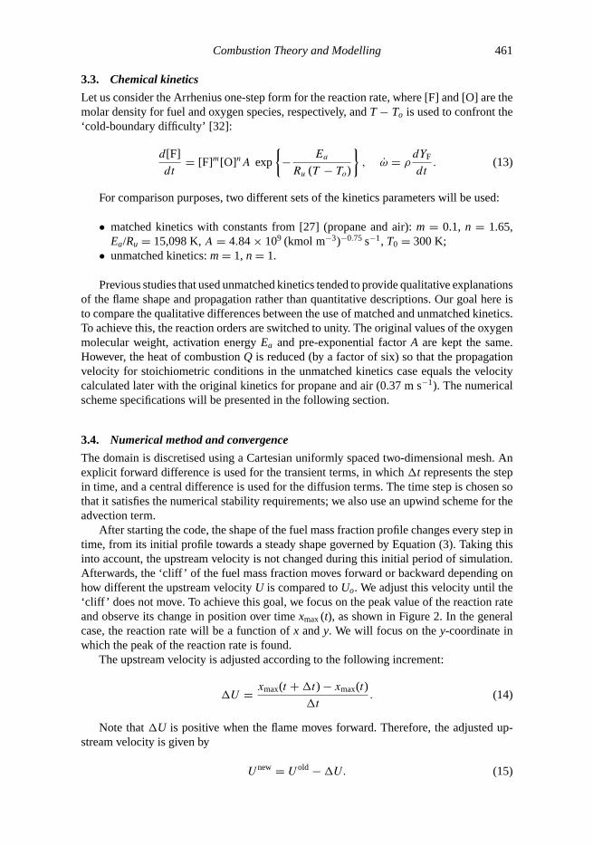
Figure 3. Scalar variables – linear equivalence ratio at the inlet (maximum equivalence ratio = 5.5).

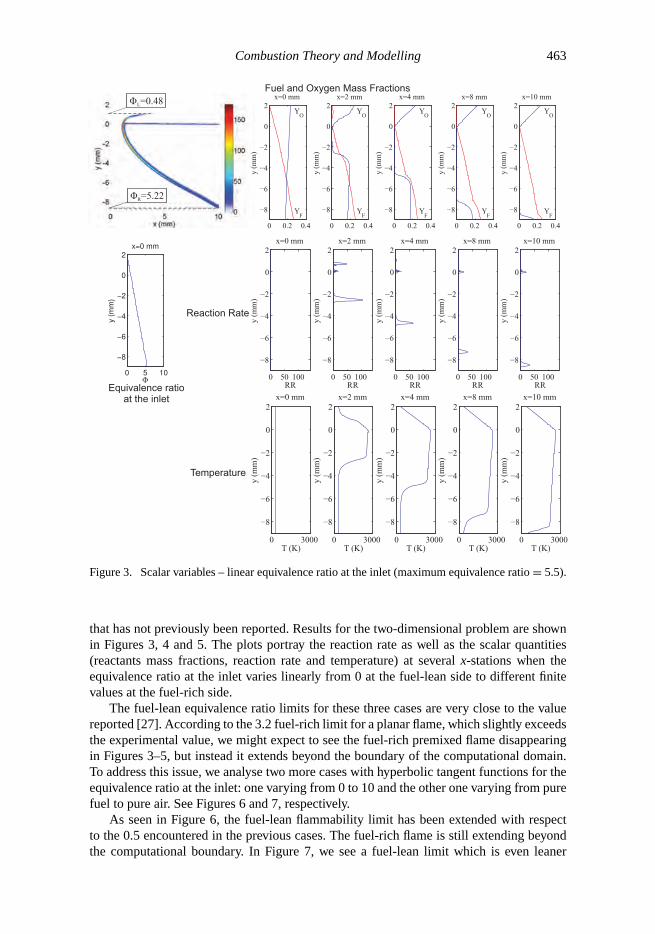
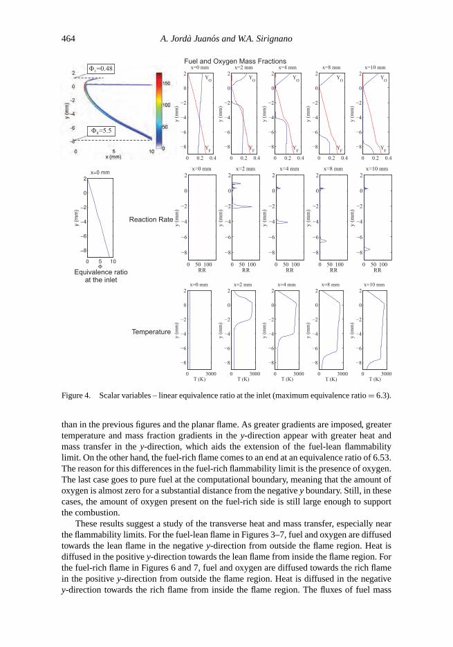
that has not previously been reported. Results for the two-dimensional problem are shownin Figures 3, 4 and 5. The plots portray the reaction rate as well as the scalar quantities(reactants mass fractions, reaction rate and temperature) at several x-stations when theequivalence ratio at the inlet varies linearly from 0 at the fuel-lean side to different finitevalues at the fuel-rich side.

The fuel-lean equivalence ratio limits for these three cases are very close to the valuereported [27]. According to the 3.2 fuel-rich limit for a planar flame, which slightly exceedsthe experimental value, we might expect to see the fuel-rich premixed flame disappearingin Figures 3–5, but instead it extends beyond the boundary of the computational domain.To address this issue, we analyse two more cases with hyperbolic tangent functions for theequivalence ratio at the inlet: one varying from 0 to 10 and the other one varying from purefuel to pure air. See Figures 6 and 7, respectively.

As seen in Figure 6, the fuel-lean flammability limit has been extended with respectto the 0.5 encountered in the previous cases. The fuel-rich flame is still extending beyondthe computational boundary. In Figure 7, we see a fuel-lean limit which is even leaner


Figure 4. Scalar variables – linear equivalence ratio at the inlet (maximum equivalence ratio = 6.3).

than in the previous figures and the planar flame. As greater gradients are imposed, greatertemperature and mass fraction gradients in the y-direction appear with greater heat andmass transfer in the y-direction, which aids the extension of the fuel-lean flammabilitylimit. On the other hand, the fuel-rich flame comes to an end at an equivalence ratio of 6.53.The reason for this differences in the fuel-rich flammability limit is the presence of oxygen.The last case goes to pure fuel at the computational boundary, meaning that the amount ofoxygen is almost zero for a substantial distance from the negative y boundary. Still, in thesecases, the amount of oxygen present on the fuel-rich side is still large enough to supportthe combustion.

These results suggest a study of the transverse heat and mass transfer, especially nearthe flammability limits. For the fuel-lean flame in Figures 3–7, fuel and oxygen are diffusedtowards the lean flame in the negative y-direction from outside the flame region. Heat isdiffused in the positive y-direction towards the lean flame from inside the flame region. Forthe fuel-rich flame in Figures 6 and 7, fuel and oxygen are diffused towards the rich flamein the positive y-direction from outside the flame region. Heat is diffused in the negativey-direction towards the rich flame from inside the flame region. The fluxes of fuel mass


Figure 5. Scalar variables – linear equivalence ratio at the inlet (maximum equivalence ratio =8.75).

fraction in the x- and y-directions, Fx and Fy respectively, are defined in Equations (16):

Fx =∣∣∣∣UYF − D

∂YF

∂x

∣∣∣∣ , Fy =∣∣∣∣D∂YF

∂y

∣∣∣∣ . (16)

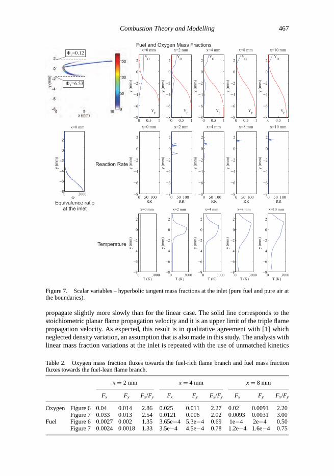
The fluxes of the oxygen mass fraction are calculated in the same fashion by replacing byoxygen in Equations (16). Table 2 shows computations of such fluxes for Figures 6 and 7 atseveral x-positions. Calculations are made at the flame front. The evolution in x of the ratiobetween the fluxes in the x-direction to the y-direction shows that the premixed branchestend to develop some diffusion character with increasing downstream distance. Althoughthe hyperbolic tangent profile has Fy decreasing with increasing y magnitude, the ratioFx/Fy at the flame front is generally decreasing which implies an increasing dependenceon transverse diffusion as the flammability limits are approached. This diffusion allowsextension of the limits. This character is identified here as the pentasectional character ofthe triple flame. Essentially, each ‘premixed’ branch of the flame can be divided into two


Figure 6. Scalar variables – hyperbolic tangent mass fractions at the inlet (maximum equivalenceratio = 10).

sections: one section near stoichiometric conditions which is predominantly premixed anda section near the flammability limits where a combined diffusion and premixed characterexists. Computations of the same fluxes at the trailing diffusion flame show clear dominanceof diffusion transport in the y-direction, as expected because it is a pure diffusion flame.

4.2. Flame structure and propagation

A qualitative analysis of the flame propagation features and shape is presented in thissection.

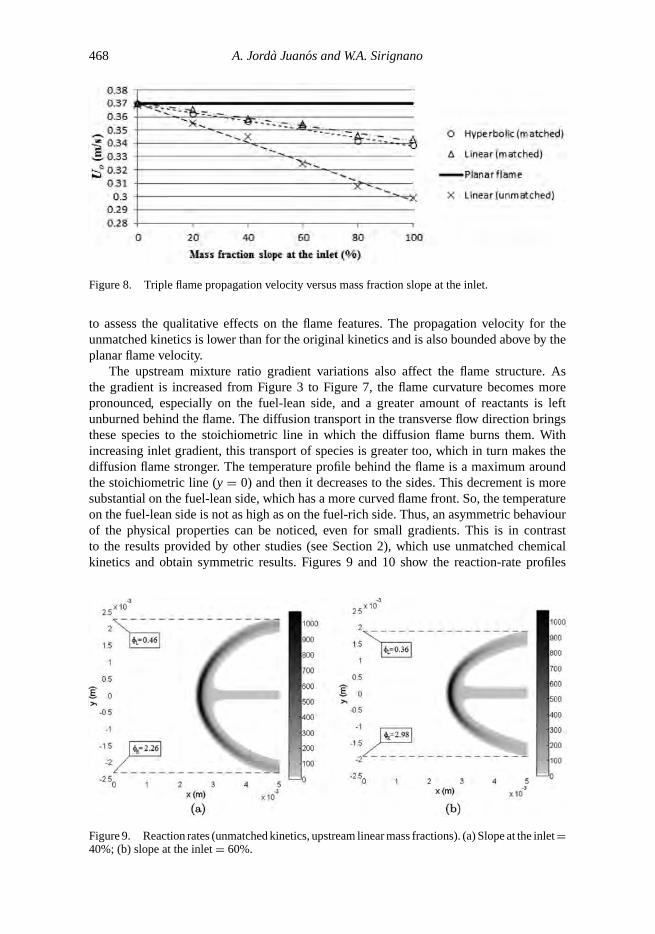
Figure 8 shows the flame propagation velocity versus upstream mixture gradient forboth the linear and hyperbolic tangent functions for the reactant mass fractions at theinlet. The slope percentage shown in the abscissa axis is based on the maximum linearslope of the upstream fuel mass fraction. The dashed lines are least square fits to thenumerical data. It can be seen how the triple-flame propagation velocity decreases as themixture gradient is increased. The flame with hyperbolic functions at the inlet is found to


Figure 7. Scalar variables – hyperbolic tangent mass fractions at the inlet (pure fuel and pure air atthe boundaries).

propagate slightly more slowly than for the linear case. The solid line corresponds to thestoichiometric planar flame propagation velocity and it is an upper limit of the triple flamepropagation velocity. As expected, this result is in qualitative agreement with [1] whichneglected density variation, an assumption that is also made in this study. The analysis withlinear mass fraction variations at the inlet is repeated with the use of unmatched kinetics

Table 2. Oxygen mass fraction fluxes towards the fuel-rich flame branch and fuel mass fractionfluxes towards the fuel-lean flame branch.

x = 2 mm x = 4 mm x = 8 mm

Fx Fy Fx/Fy Fx Fy Fx/Fy Fx Fy Fx/Fy

Oxygen Figure 6 0.04 0.014 2.86 0.025 0.011 2.27 0.02 0.0091 2.20Figure 7 0.033 0.013 2.54 0.0121 0.006 2.02 0.0093 0.0031 3.00

Fuel Figure 6 0.0027 0.002 1.35 3.65e−4 5.3e−4 0.69 1e−4 2e−4 0.50Figure 7 0.0024 0.0018 1.33 3.5e−4 4.5e−4 0.78 1.2e−4 1.6e−4 0.75


Figure 8. Triple flame propagation velocity versus mass fraction slope at the inlet.

to assess the qualitative effects on the flame features. The propagation velocity for theunmatched kinetics is lower than for the original kinetics and is also bounded above by theplanar flame velocity.

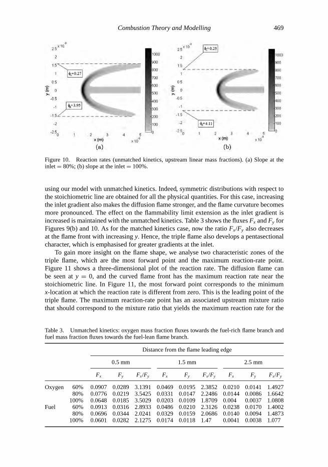
The upstream mixture ratio gradient variations also affect the flame structure. Asthe gradient is increased from Figure 3 to Figure 7, the flame curvature becomes morepronounced, especially on the fuel-lean side, and a greater amount of reactants is leftunburned behind the flame. The diffusion transport in the transverse flow direction bringsthese species to the stoichiometric line in which the diffusion flame burns them. Withincreasing inlet gradient, this transport of species is greater too, which in turn makes thediffusion flame stronger. The temperature profile behind the flame is a maximum aroundthe stoichiometric line (y = 0) and then it decreases to the sides. This decrement is moresubstantial on the fuel-lean side, which has a more curved flame front. So, the temperatureon the fuel-lean side is not as high as on the fuel-rich side. Thus, an asymmetric behaviourof the physical properties can be noticed, even for small gradients. This is in contrastto the results provided by other studies (see Section 2), which use unmatched chemicalkinetics and obtain symmetric results. Figures 9 and 10 show the reaction-rate profiles

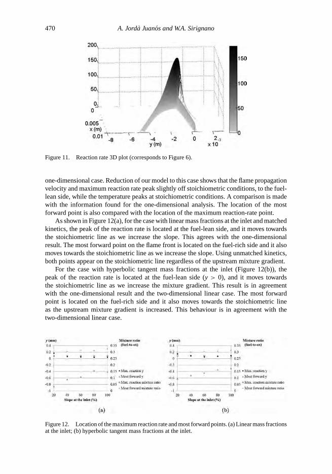
Figure 9. Reaction rates (unmatched kinetics, upstream linear mass fractions). (a) Slope at the inlet =40%; (b) slope at the inlet = 60%.


Figure 10. Reaction rates (unmatched kinetics, upstream linear mass fractions). (a) Slope at theinlet = 80%; (b) slope at the inlet = 100%.

using our model with unmatched kinetics. Indeed, symmetric distributions with respect tothe stoichiometric line are obtained for all the physical quantities. For this case, increasingthe inlet gradient also makes the diffusion flame stronger, and the flame curvature becomesmore pronounced. The effect on the flammability limit extension as the inlet gradient isincreased is maintained with the unmatched kinetics. Table 3 shows the fluxes Fx and Fy forFigures 9(b) and 10. As for the matched kinetics case, now the ratio Fx/Fy also decreasesat the flame front with increasing y. Hence, the triple flame also develops a pentasectionalcharacter, which is emphasised for greater gradients at the inlet.

To gain more insight on the flame shape, we analyse two characteristic zones of thetriple flame, which are the most forward point and the maximum reaction-rate point.Figure 11 shows a three-dimensional plot of the reaction rate. The diffusion flame canbe seen at y = 0, and the curved flame front has the maximum reaction rate near thestoichiometric line. In Figure 11, the most forward point corresponds to the minimumx-location at which the reaction rate is different from zero. This is the leading point of thetriple flame. The maximum reaction-rate point has an associated upstream mixture ratiothat should correspond to the mixture ratio that yields the maximum reaction rate for the

Table 3. Unmatched kinetics: oxygen mass fraction fluxes towards the fuel-rich flame branch andfuel mass fraction fluxes towards the fuel-lean flame branch.

Distance from the flame leading edge

0.5 mm 1.5 mm 2.5 mm

Fx Fy Fx/Fy Fx Fy Fx/Fy Fx Fy Fx/Fy

Oxygen 60% 0.0907 0.0289 3.1391 0.0469 0.0195 2.3852 0.0210 0.0141 1.492780% 0.0776 0.0219 3.5425 0.0331 0.0147 2.2486 0.0144 0.0086 1.6642

100% 0.0648 0.0185 3.5029 0.0203 0.0109 1.8709 0.004 0.0037 1.0808Fuel 60% 0.0913 0.0316 2.8933 0.0486 0.0210 2.3126 0.0238 0.0170 1.4002

80% 0.0696 0.0344 2.0241 0.0329 0.0159 2.0686 0.0140 0.0094 1.4873100% 0.0601 0.0282 2.1275 0.0174 0.0118 1.47 0.0041 0.0038 1.077


Figure 11. Reaction rate 3D plot (corresponds to Figure 6).

one-dimensional case. Reduction of our model to this case shows that the flame propagationvelocity and maximum reaction rate peak slightly off stoichiometric conditions, to the fuel-lean side, while the temperature peaks at stoichiometric conditions. A comparison is madewith the information found for the one-dimensional analysis. The location of the mostforward point is also compared with the location of the maximum reaction-rate point.

As shown in Figure 12(a), for the case with linear mass fractions at the inlet and matchedkinetics, the peak of the reaction rate is located at the fuel-lean side, and it moves towardsthe stoichiometric line as we increase the slope. This agrees with the one-dimensionalresult. The most forward point on the flame front is located on the fuel-rich side and it alsomoves towards the stoichiometric line as we increase the slope. Using unmatched kinetics,both points appear on the stoichiometric line regardless of the upstream mixture gradient.

For the case with hyperbolic tangent mass fractions at the inlet (Figure 12(b)), thepeak of the reaction rate is located at the fuel-lean side (y > 0), and it moves towardsthe stoichiometric line as we increase the mixture gradient. This result is in agreementwith the one-dimensional result and the two-dimensional linear case. The most forwardpoint is located on the fuel-rich side and it also moves towards the stoichiometric lineas the upstream mixture gradient is increased. This behaviour is in agreement with thetwo-dimensional linear case.

Figure 12. Location of the maximum reaction rate and most forward points. (a) Linear mass fractionsat the inlet; (b) hyperbolic tangent mass fractions at the inlet.


5. Conclusions

A numerical two-dimensional analysis has been presented to model triple flames. Theresults reflect that imposition of greater transverse mixture ratios extend the flammabilitylimits beyond those corresponding to a planar flame. This result is due to an increasedtransport of heat and mass in the transverse direction of the flow. Studying the mass fluxesof the reactants towards the lateral ‘premixed’ flame branches shows that they evolvefrom premixed flames at near stoichiometric conditions to a combination of premixedand diffusion flames near the flammability limits. So, each ‘premixed’ branch can beseparated into two sections, which is identified as the pentasectional character of thetriple flame.

Linear and hyperbolic tangent functions of the transverse coordinate have been usedto prescribe the equivalence ratio or the reactants mass fractions at the inlet. Linear andhyperbolic tangent variations of inflowing mass fractions produce qualitatively similarresults. The flame propagation speed has a limiting value, which corresponds to the planarpremixed flame speed; the propagation velocity is slightly higher for the linear case than forthe hyperbolic case; increasing the upstream transverse mixture gradient causes a reductionof the triple-flame propagation velocity and an increase of the flame front curvature; theflame front shape is highly asymmetric with respect to the stoichiometric line; the maximumreaction-rate point is located at the fuel-lean side, while the triple flame leading point islocated at the fuel-rich side. Both points get closer to the stoichiometric line as the upstreammixture gradient is increased. Using unmatched chemical kinetics with unitary mass fractionexponents results in symmetric flame structures with respect to the stoichiometric line, andmaximum reaction rate and most forward points located at the stoichiometric line. Thus,the use of unmatched kinetics leads to solutions that do not represent qualitatively real tripleflame structure. However, flammability limit extension and pentasectional character of thetriple flame still appear.

Even though the heat release effects have been relaxed, the work presented in this papershows the importance of using experimental chemical kinetics data. Heat release causesthe streamlines ahead of the flame to diverge due to gas expansion, which at the same timecauses the mixture gradient to decrease, especially around the stoichiometric line whereheat release effects are more pronounced. The mixture gradient strength increases againfarther away from the stoichiometric line, where the streamlines become more parallel.These consequences on the mixture gradient along the flame front would cause changes inthe solutions for the flame structure if gas expansion due to heat release were considered.However, asymmetries of the flame front associated with the use of experimental kineticswould still be expected.

A suggested further refinement of the present modelling would be to take densityvariation into consideration together with the use of experimental chemical kinetics data.More accurate chemical kinetics mechanisms (i.e. multiple-step) would also be desir-able, as well as considering suitable non-unity Lewis numbers. A study accounting forthese new assumptions together with the imposition of a velocity gradient at the in-let would be expected to affect the x-coordinate at which the flame may be stabilised.Simulations performed in such a study would be helpful for the design of combustionchambers.

FundingThe first author appreciates Balsells Fellowship support.


References[1] J.W. Dold, Flame propagation in a nonuniform mixture: Analysis of a slowly varying triple

flame, Combust. Flame 76 (1989), pp. 71–88.[2] J. Buckmaster and M. Matalon, Anomalous Lewis number effects in tribrachial flames, Proc.

Combust. Inst. 22 (1988), pp. 1527–1535.[3] S. Ghosal and L. Vervisch, Theoretical and numerical study of a symmetrical triple flame using

the parabolic flame path approximation, J. Fluid Mech. 415 (2000), pp. 227–260.[4] H. Phillips, Flame in a buoyant methane layer, Symp. (Int.) Combust. 10 (1965), pp. 1277–

1283.[5] S.H. Chung and B.J. Lee, On the characteristics of laminar lifted flames in a nonpremixed jet,

Combust. Flame 86 (1991), pp. 62–72.[6] P.N. Kioni, B. Rogg, K.N.C. Bray, and A. Linan, Flame spread in laminar mixing layers: The

triple flame, Combust. Flame 95 (1993), pp. 276–290.[7] B.J. Lee, J.S. Kim, and S.H. Chung, Effect of dilution of the liftoff of nonpremixed jet flames,

Proc. Combust. Inst. 25 (1994), pp. 1175–1181.[8] B.J. Lee and S.H. Chung, Stabilization of lifted tribrachial flames in a laminar nonpremixed

jet, Combust. Flame 109 (1997), pp. 163–172.[9] T. Plessing, P. Terhoeven, N. Peters, and M.S. Mansour, An experimental and numerical study

of a laminar triple flame, Combust. Flame 115 (1998), pp. 335–353.[10] Y.S. Ko, T.M. Chung, and S.H. Chung, Characteristics of propagating tribrachial flames in

counterflow, KSME Int. J. 16 (2002), pp. 1710–1718.[11] T.K. Pham, D. Dunn-Rankin, and W.A. Sirignano, Flame structure in small-scale liquid film

combustors, Proc. Combust. Inst. 31 (2006), pp. 3269–3275.[12] S.H. Chung, Stabilization, propagation and instability of tribrachial triple flames, Proc. Com-

bust. Inst. 31 (2007), pp. 877–892.[13] J.R. Bellan and W.A. Sirignano, A theory of turbulent flame development and nitric oxide

formation in stratified charge internal combustion engines, Combust. Sci. Technol. 8 (1973),pp. 51–68.

[14] N. Peters, Laminar flamelet concepts in turbulent combustion, Symp. (Int.) Combust. 21 (1988),pp. 1231–1250.

[15] J.W. Dold, L.J. Hartley, and D. Green, Dynamics of laminar triple-flamelet structures in non-premixed turbulent combustion, in Dynamical Issues in Combustion Theory, P.C. Fife, A. Linan,and F. Williams, eds., The IMA Volumes in Mathematics and its Applications Vol. 35, Springer,New York, 1991, pp. 83–105. Available at http://dx.doi.org/10.1007/978-1-4612-0947-8_4.

[16] J.Y. Chen and T. Echekki, Numerical study of buoyancy effects on triple flames, Western StatesSpring Meeting, The Combustion Institute, 13–14 March 2000, Paper number WS 00S-11.

[17] L.J. Hartley and J.W. Dold, Flame propagation in a nonuniform mixture: Analysis of a propa-gating triple flame, Combust. Sci. Technol. 80 (1991), pp. 23–46.

[18] G.R. Ruetsch, L. Vervisch, and A. Linan, Effects of heat release on triple flames, Phys. Fluids7 (1995), pp. 1447–1454.

[19] P. Domingo and L. Vervisch, Triple flames and partially premixed combustion in autoignitionof non-premixed turbulent mixtures, Proc. Combust. Inst. 26 (1996), pp. 233–240.

[20] T.G. Vedarajan and J. Buckmaster, Edge-flames in homogeneous mixtures, Combust. Flame114 (1998), pp. 267–273.

[21] J. Daou and A. Linan, Triple flames in mixing layers with nonunity Lewis numbers, Symp. (Int.)Combust. 27 (1998), pp. 667–674.

[22] T. Echekki and J.H. Chen, Structure and propagation of methanol-air triple flames – physi-cal and chemical fundamentals, modeling and simulation, experiments, pollutant formation,Combust. Flame 114 (1998), pp. 231–245.

[23] H.G. Im and J.H. Chen, Structure and propagation of triple flames in partially premixedhydrogen–air mixtures, Combust. Flame 119 (1999), pp. 436–454.

[24] H.G. Im and J.H. Chen, Effects of flow strain on triple flame propagation, Combust. Flame 126(2001), pp. 1384–1392.

[25] E. Fernandez, M. Vera, and A. Linan, Liftoff and blowoff of a diffusion flame between parallelstreams of fuel and air, Combust. Flame 144 (2005), pp. 261–276.

[26] C. Jimenez and B. Cuenot, DNS study of stabilization of turbulent triple flames by hot gases,Proc. Combust. Inst. 31 (2007), pp. 1649–1656.

[27] C.K. Westbrook and F.L. Dryer, Chemical kinetic modeling of hydrocarbon combustion, Prog.Energy Combust. Sci. 10 (1984), pp. 1–57.


[28] J. Buckmaster, Edge-flames, Prog. Energy Combust. Sci. 28 (2002), pp. 435–475.[29] S.R. Turns, An Introduction to Combustion Concepts and Applications, 3rd ed., McGraw-Hill

Science/Engineering/Math, New York. 2011.[30] N.D. Sandham and W.C. Reynolds, Compressible mixing layer: Linear theory and direct

simulation, AIAA J. 28 (1990), pp. 618–624.[31] M. Zhuang, T. Kubota, and P.E. Dimotakis, Instability of inviscid, compressible free shear

layers, AIAA J. 28 (1990), pp. 1728–1733.[32] H. Berestycki, B. Larrouturou, and J. Roquejoffre, Mathematical investigation of the

cold boundary difficulty in flame propagation theory, in Dynamical Issues in Combus-tion Theory, P.C. Fife, A. Linan, and F. Williams, eds., The IMA Volumes in Mathe-matics and its Applications Vol. 35, Springer, New York, 1991, pp. 37–61. Available athttp://dx.doi.org/10.1007/978-1-4612-0947-8_2.

Documents

Triple flame: Inherent asymmetries and pentasectional