Embed Size (px)
Citation preview
COMPETITIVE OPTIMISATION ON TIMED AUTOMATA
BY
ASHUTOSH TRIVEDI
A THESIS SUBMITTED IN PARTIAL FULFILMENT OF THE
REQUIREMENTS FOR THE DEGREE
OFDOCTOR OF PHILOSOPHY IN COMPUTER SCIENCE
UNIVERSITY OF WARWICK, DEPARTMENT OF COMPUTER SCIENCE
APRIL 2009
To Tiziana, for maximising happiness and minimising troubles, andto Miralisa, for playing two-player zero-sum games with me.
Contents
List of Figures iv
List of Tables v
Acknowledgement vi
Declaration vii
Abstract viii
Chapter 1. Introduction 11.1. Motivation 11.2. Preliminaries: Dynamic Programming and Game Theory 31.3. Literature Review 91.4. Contributions of the Thesis 151.5. Organisation of the Thesis 17
Part 1. Background 19
Chapter 2. Competitive Optimisation on Finite Graphs 202.1. Formal Definition 202.2. Noncompetitive Optimisation on Finite Graphs 222.3. Games on Finite Graphs 372.4. Discussion 46
Chapter 3. Timed Automata 483.1. Examples 493.2. Formal Definition 503.3. Some Properties of Regions 533.4. Extensions of Timed Automata 553.5. Competitive Optimisation on Timed Automata 593.6. A Note on Zeno Runs 633.7. Abstractions of Timed Automata 64
Part 2. Competitive Optimisation on Timed Automata 71
Chapter 4. Noncompetitive Optimisation 72ii
CONTENTS iii
4.1. Concavely-Priced Timed Automata 724.2. Optimisation Problems on Priced Timed Automata 734.3. Region Graphs 744.4. Correctness of the Boundary Region Graph Abstraction 774.5. Concave-Regularity of Cost Functions 82
Chapter 5. Reachability-Time Games 885.1. Introduction 885.2. Simple Functions 915.3. Reachability-Time Games on Boundary Region Automata 925.4. Solving Optimality Equations by Strategy Improvement 965.5. Complexity 102
Chapter 6. Average-Time Games 1056.1. Introduction 1056.2. Abstractions of Timed Automata 1076.3. Strategies in Region Graphs 1106.4. Average-Time Games on Region Graphs 1186.5. Complexity 122
Part 3. Conclusion 124
Chapter 7. Summary and Future Work 1257.1. Summary 1257.2. Future Work 126
Part 4. Appendix 129
Appendix A. Notations and Acronyms 130
Appendix B. Results From Real Analysis 136B.1. Lipschitz-Continuous Functions 136B.2. Concave and Quasiconcave Functions 137B.3. Fixed Point Theorems 139
Appendix C. Some Determinacy Results 140C.1. Matrix Games 140C.2. Stopping Stochastic Games 142
Appendix D. Implementation Details 144D.1. Lexer 144D.2. Parser 145
Bibliography 148
Index 152
List of Figures
1.1 An artificial heart-pacemaker. 3
1.2 Pseudocode of a Value Iteration Method. 6
1.3 Pseudocode of a Policy Iteration Method. 6
1.4 Value Iteration Algorithm to Solve Opt√(S). 7
2.1 A priced finite graph with final vertices. 21
2.2 Strategy improvement algorithm to solve OERPMin(G). 27
2.3 Strategy improvement algorithm to solve OEDPMin(G, λ). 31
2.4 A finite price-reward graph. 34
2.5 Strategy improvement algorithm to solve OEPRAvgMin (G) . 35
2.6 Strategy improvement algorithm to solve OERPMinMax(G). 42
2.7 Strategy improvement algorithm to solve OEDPMinMax(G, λ) . 44
2.8 Strategy improvement algorithm to solve OEPRAvgMinMax(G). 46
3.1 A light-bulb modelled using a timed automaton. 49
3.2 A timed automaton with more than one clock. 49
3.3 Clock regions of a timed automaton. 51
3.4 A Zeno Timed Automaton. 63
3.5 Evolution of regions in a corner-point abstraction of a timed automaton (the idea ofthis figure is from Bouyer [Bou06]). 66
3.6 Evolution of regions in a boundary region graph of a timed automaton. 69
5.1 Strategy improvement algorithm for OERTMax(ΓBR). 99
5.2 Strategy improvement algorithm for solving OERTMinMax(ΓBR). 102
5.3 A Reduction from a Countdown Game to a Reachability Game. 103
6.1 A Reduction from a Countdown Game to an Average-Time Game. 123
iv
List of Tables
1 General Notations 131
2 Standard Notations related to minmum, infimum, and argmin. 131
3 Non-standard notations related to minimum, infimum, and argmin 132
4 Notations specific to timed automata 134
5 Acronyms 135
v
Acknowledgement
First of all, I wish to express my gratitude to my supervisor Dr. Marcin Jurdzinski. Hispassion for mathematical rigour and elegance is the inspiration behind every significantdiscovery made during the research presented in this thesis. His patience, his timely advice,his encouragements, his belief in my abilities, and his continuous support through some ofthe difficult moments of my life, helped me and this thesis in uncountably infinite ways.
I am thankful to my adviser Dr. Ranko Lazic for ensuring safety, liveness, and fairnessproperties of my Ph.D. programme.
I would like to acknowledge my Ph.D. examiners Dr. Joel Ouaknine and Dr. Ranko Lazicfor insightful comments on my thesis.
Sincere gratitude is extended to Prof. Doron Peled for his invaluable time and guidanceduring my first year at Warwick. I also thank him for his help during the admission processand for the financial support for my Ph.D. studies.
I would like to thank the support staff at the department of computer science and at thelibrary services of the University of Warwick.
I wish to thank Prof. Marta Kwiatkowska for her help and support during my transitionfrom a Ph.D. student to a postdoc researcher.
Special thanks to my friend Nick Papanikolaou for his constructive criticism of myideas, and for various other discussions on some undecidable problems. I thank followingcolleagues for providing a stimulating and enjoyable atmosphere in the department ofcomputer science: Haris Aziz, Timothy Davidson, Alexander Dimovski, John Fearnly, AntonyHolmes, Ritesh Krishna, Hongyang Qu, Michał Rutkowski, and Daniel Valdes-Amaro.
I would like to thank all my friends for such an enjoyable time at Warwick. I wouldparticularly like to mention: Diana Apiyo, Rajesh S. Balakrishnan, Massoumeh Dashti, EstelleGuyez/Picard, Samuel Lelievre, Eleftheria Papoulia, Serena Pattaro, Tina Philip, Jothi Philip, CyrilPicard, Leslie Robinson, and Agnieszka Rutkowska. Also, thanks to my friends, Amol Patil andMonica Mantri, for some great time at Oxford.
I am fortunate to have a loving, caring, and ever supporting family. This acknowledge-ment is incomplete without thanking all of them: papa (Suresh Chandra Trivedi), mummy(Bharti Trivedi), didi (Bhawana Katyayan), jijaji (Amogh Katyayan), dada (Vibhor Vibhu Trivedi),bhabhiji (Anjali Trivedi), and Richa (Richa Trivedi). Special thanks to my mother-in-lawFranca Beatrice Girardi for her love and support.
Finally I would like to dedicate this thesis to my wife Tiziana, for maximising happinessand minimising troubles, and to my daughter Miralisa, for playing two-player zero-sumgames with me.
vi
Declaration
This thesis is presented in accordance with the regulations for the degree of Doctor ofPhilosophy. It has been composed by myself and has not been submitted in any previousapplication for any degree. The work in this thesis has been undertaken by myself underthe supervision of Dr. Marcin Jurdzinski.
Although the key results of the thesis have been announced in proceedings of someinternational conferences, this thesis presents the results with complete proofs and comple-ments them with illustrations.
Chapter 4 (Noncompetitive Optimisation) is an extended version of the paper Concavely-Priced Timed Automata [JT08b], which appeared in the proceedings of the conference onformal modelling and analysis of timed systems (FORMATS) 2008.
Chapter 5 (Reachability-Time Games) is an extended version of the paper Reachability-Time Games on Timed Automata [JT07], which appeared in the proceedings of internationalcolloquium on automata, languages and programming (ICALP) 2007.
Chapter 6 (Average-Time Games) is an extended version of the paper Average-TimeGames [JT08a], which appeared in the proceedings of the IARCS Annual Conference onFoundations of Software Technology and Theoretical Computer Science (FSTTCS) 2008.
vii
Abstract
Timed automata are finite automata accompanied by a finite set of real-valued variablescalled clocks. Optimisation problems on timed automata are fundamental to the verificationof properties of real-time systems modelled as timed automata, while the control-programsynthesis problem of such systems can be modelled as a two-player game. This thesispresents a study of optimisation problems and two-player games on timed automata undera general heading of competitive optimisation on timed automata.
This thesis views competitive optimisation on timed automata as a multi-stage decisionprocess, where one or two players are confronted with the problem of choosing a sequenceof timed moves—a time delay and an action—in order to optimise their objectives. Asolution of such problems consists of the “optimal” value of the objective and an “optimal”strategy for each player. This thesis introduces a novel class of strategies, called boundarystrategies, that suggest to a player a symbolic timed move of the form (b, c, a)— “wait untilthe value of the clock c is in very close proximity of the integer b, and then execute atransition labelled with the action a”. A distinctive feature of the competitive optimisationproblems discussed in this thesis is the existence of optimal boundary strategies. Surprisinglyperhaps, many competitive optimisation problems on timed automata of practical interestadmit optimal boundary strategies. For example, optimisation problems with reachabilityprice, discounted price, and average-price objectives, and two-player turn-based gameswith reachability time and average time objectives.
The existence of optimal boundary strategies allows one to work with a novel abstrac-tion of timed automata, called a boundary region graph, where players can use only boundarystrategies. An interesting property of a boundary region graph is that, for every state, theset of reachable states is finite. Hence, the existence of optimal boundary strategies permitsus to reduce competitive optimisation problem on a timed automaton to the correspondingcompetitive optimisation problem on a finite graph.
viii
1Introduction
Pessimism is, in brief, playingthe sure game. You cannot loseat it; you may gain. It is the onlyview of life in which you cannever be disappointed. Havingreckoned what to do in theworst possible circumstances,when better arise, as they may,life becomes child’s play.
Thomas Hardy
Timed automata are finite automata accompanied by a finite set of real-valued vari-ables. Optimisation problems on timed automata are fundamental to the verification of(quantitative timing) properties of systems modelled as timed automata. On the otherhand, the problem of control-program synthesis of systems modelled as timed automatacan be cast as a two-player game—where the two players correspond to the “controller”and the “environment”—and the control-program synthesis corresponds to computingwinning (or optimal) strategies for the controller. We study optimisation problems andtwo-player games on timed automata under a general heading of competitive optimisationon timed automata. The theory of dynamic programming provides concepts and algorithmsto analyse optimisation problems on multi-stage decision processes. We argue thatdynamic programming is an effective tool to design and analyse algorithms for competitiveoptimisation on timed automata.
1.1. MotivationThis research has theoretical as well as practical motivations: algorithms for the competitiveoptimisation on timed automata provide upper bounds on the computational complexityof such problems. On the practical side, these algorithms are useful for the verification andcontroller synthesis of real-time open systems. In this section, with the help of a simpleexample, we demonstrate how certain two-player games on timed automata can be used tomodel some controller-synthesis problems of real-time systems.
1
1.1. MOTIVATION 2
By a real-time open system, we mean a computer system which interacts with itsenvironment (open), and whose correctness depends critically on the time (real time) inwhich it performs some of its actions. Real-time open systems are prevalent parts of safety-critical systems, where a bug in their design can be catastrophic. Some examples [Wik09] ofsafety-critical real-time systems are artificial pacemaker, robotic surgery machine, nuclearreactor system, railway signalling and control system, aircraft-landing scheduling system,air-bag control system and satellite-launching system.
Given the safety-critical nature of the applications of real-time open systems, it is ofparamount importance to ensure their correctness.
As an example of a safety-critical real-time open system, let us consider the followingdescription of an artificial pacemaker.
The pacemaker leads detect the heart’s own electrical activity (in the right atrium and right ventricle,) andtransmit that information to the pacemaker generator. The generator—which, again, is a computer—analysesthe heart’s electrical signals, and uses that information to decide whether, when, and where to pace. If the heartrate becomes too slow, the generator transmits a tiny electrical signal to the heart, thus stimulating the heartmuscle to contract. (This is called pacing.)
Pacemakers that have two leads not only keep the heart rate from dropping too low, they can also maintainthe optimal coordination between the atria and the ventricles (by pacing the atrium and the ventricle insequence.)
Thus, pacemakers do not take over the work of the heart—the heart still does its own beating—but instead,pacemakers merely help to regulate the timing of the heart beat. (Richard N. Fogoros, M.D., Cardiology,Pittsburgh, PA)
Observe that the main function of a pacemaker is to maintain the rate of heart beatswhen the natural pacemaker of the heart is either too slow or not working due to someproblem. Artificial pacemaker is an example of real-time open systems as it interacts with itsenvironment (heart’s own electrical activity) and the correctness of its operations criticallydepends on the timing of its actions.
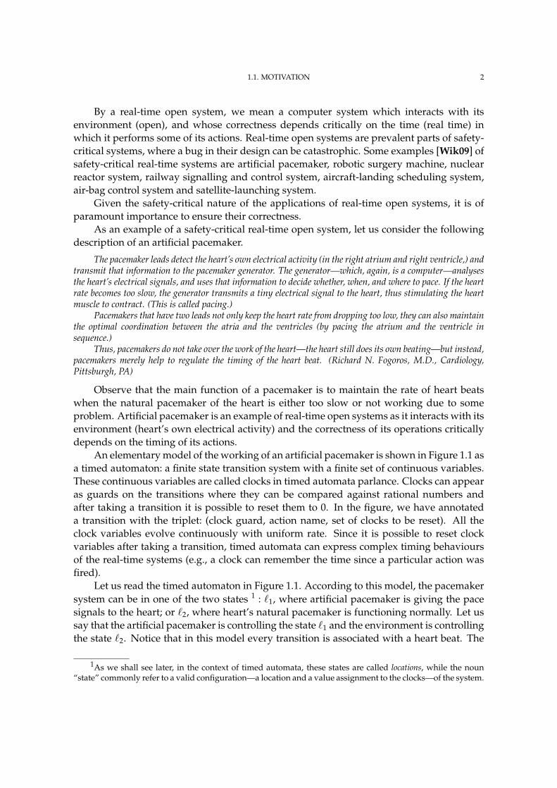
An elementary model of the working of an artificial pacemaker is shown in Figure 1.1 asa timed automaton: a finite state transition system with a finite set of continuous variables.These continuous variables are called clocks in timed automata parlance. Clocks can appearas guards on the transitions where they can be compared against rational numbers andafter taking a transition it is possible to reset them to 0. In the figure, we have annotateda transition with the triplet: (clock guard, action name, set of clocks to be reset). All theclock variables evolve continuously with uniform rate. Since it is possible to reset clockvariables after taking a transition, timed automata can express complex timing behavioursof the real-time systems (e.g., a clock can remember the time since a particular action wasfired).
Let us read the timed automaton in Figure 1.1. According to this model, the pacemakersystem can be in one of the two states 1 : `1, where artificial pacemaker is giving the pacesignals to the heart; or `2, where heart’s natural pacemaker is functioning normally. Let ussay that the artificial pacemaker is controlling the state `1 and the environment is controllingthe state `2. Notice that in this model every transition is associated with a heart beat. The
1As we shall see later, in the context of timed automata, these states are called locations, while the noun“state” commonly refer to a valid configuration—a location and a value assignment to the clocks—of the system.
1.2. PRELIMINARIES: DYNAMIC PROGRAMMING AND GAME THEORY 3
x ≥ 2, artificial beat, x, y
x ≥ 1, artificial beat, x, y
y ≤ 2, artificial beat, x, y y ≤ 1, natural beat, y
`1 `2
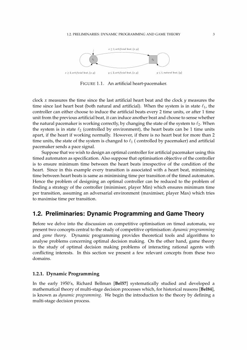
FIGURE 1.1. An artificial heart-pacemaker.
clock x measures the time since the last artificial heart beat and the clock y measures thetime since last heart beat (both natural and artificial). When the system is in state `1, thecontroller can either choose to induce the artificial beats every 2 time units, or after 1 timeunit from the previous artificial beat, it can induce another beat and choose to sense whetherthe natural pacemaker is working correctly, by changing the state of the system to `2. Whenthe system is in state `2 (controlled by environment), the heart beats can be 1 time unitsapart, if the heart if working normally. However, if there is no heart beat for more than 2time units, the state of the system is changed to `1 ( controlled by pacemaker) and artificialpacemaker sends a pace signal.
Suppose that we wish to design an optimal controller for artificial pacemaker using thistimed automaton as specification. Also suppose that optimisation objective of the controlleris to ensure minimum time between the heart beats irrespective of the condition of theheart. Since in this example every transition is associated with a heart beat, minimisingtime between heart beats is same as minimising time per transition of the timed automaton.Hence the problem of designing an optimal controller can be reduced to the problem offinding a strategy of the controller (minimiser, player Min) which ensures minimum timeper transition, assuming an adversarial environment (maximiser, player Max) which triesto maximise time per transition.
1.2. Preliminaries: Dynamic Programming and Game Theory
Before we delve into the discussion on competitive optimisation on timed automata, wepresent two concepts central to the study of competitive optimisation: dynamic programmingand game theory. Dynamic programming provides theoretical tools and algorithms toanalyse problems concerning optimal decision making. On the other hand, game theoryis the study of optimal decision making problems of interacting rational agents withconflicting interests. In this section we present a few relevant concepts from these twodomains.
1.2.1. Dynamic Programming
In the early 1950’s, Richard Bellman [Bel57] systematically studied and developed amathematical theory of multi-stage decision processes which, for historical reasons [Bel84],is known as dynamic programming. We begin the introduction to the theory by defining amulti-stage decision process.
1.2. PRELIMINARIES: DYNAMIC PROGRAMMING AND GAME THEORY 4
1.2.1.1. Multi-stage Decision Processes
Multi-stage decision processes [Bel57, How60, Ber95] are the systems where a decisionmaker or a player is confronted with a problem of making sequential decisions of choosingactions in order to optimise a certain objective. We assume that every action is associatedwith a fixed price—a real number. Starting with the initial state of the system, at the firststage the player chooses an action as a result of which the state of the system is modified.In the next stage, the player makes the decision from the resulting state and the state of thesystem is modified accordingly. The total number of stages, also called the horizon, can befinite or infinite. The total cost of the sequence of actions over the horizon is a function of theprices of the individual actions. We refer to this function as the cost function. The goal of theplayer is to make decisions in such a way that it minimises (or maximises) the cost function.An important characteristic of such processes is that the decision made at any stage not onlyaffects the immediate price, but also affects the future states and hence individual decisionscan not be viewed in isolation.
Various multi-stage decision processes can succinctly be specified as optimisationproblems on mathematical formalisms such as graphs, Markov decision processes [Put94],timed automata [AD90, CY92, BBL04, BBBR07], etc.
1.2.1.2. Strategies and Value
The optimisation problem for a multi-stage decision processes is to suggest a rule of making“allowable decisions” to the player so that no other sequence of allowable decisions yields abetter value of the cost function. Such rule often takes the form of a function from the set ofhistories of decisions (sequence of visited states and executed actions) to the set of actions,and we call such a function a policy or a strategy.
Let S be the set of states and let A be the set of actions of a multi-stage decisionprocess M. For a state s, let A(s) be the set of allowable actions from the state s. Letπ : S× A → R be the price function such that for every state s ∈ S and action a ∈ A(s),π(s, a) gives the fixed-price of taking action a from the state s.
A strategy σ is then a function (S × A)∗ × S → A such that for every history h =〈s1, a2, s2, . . . , an, sn〉 ∈ (S × A)∗ × S we have σ(h) ∈ A(sn). Let us write Σ for the set ofstrategies. For a given strategy σ, we define its value Val(σ) : S → R such that Val(σ)(s) isthe value of the cost function if the initial state is s and the decisions are made according tothe strategy σ.
We say that a strategy σ∗ is optimal if for every strategy σ ∈ Σ we have that Val(σ∗)(s) ≤Val(σ)(s), for every state s. We define the optimum value as the value of the optimal strategy.
Given a multi-stage decision process, the optimisation problem is to find an optimalpolicy and the optimum value. The main tool in dynamic programming is to characterisethe optimum value by a set of functional equation called optimality equations.
1.2.1.3. Optimality Equations
Bellman observed [Bel57] that optimal policies (strategies) for a number of multi-stagedecision processes follow the following principle.
1.2. PRELIMINARIES: DYNAMIC PROGRAMMING AND GAME THEORY 5
The Principle of Optimality: An optimal policy has the property that whatever the initial state and initialdecision are, the remaining decisions must constitute an optimal policy with regard to the state resulting fromthe first decision.
This principle states that the global optimality has certain local behaviour. This factis mathematically captured by designing a set of functional equations which connect theoptimum value of a state with the optimum values of its successor states. We call theseequations optimality equations [Ber95, Bel57]. Other popular names for these equations areBellman equations, functional equations, and dynamic programming equations.
To solve an optimisation problem of multi-stage decision processes using dynamicprogramming [Put94] we need to: a) design a set of optimality equations, b) formally provethat given a solution of such equations one can easily compute an optimal policy and theoptimum value, and c) design an algorithm to solve these equations.
Once we have the right optimality equations, the next step is to prove the existencetheorem (i.e., that there exists a solution of these equations). A constructive proof of theexistence theorem can be given by writing an algorithm to solve optimality equations.Sometimes it is also possible to prove the uniqueness theorem (i.e., that the solution of theoptimality equations is unique).
1.2.1.4. Solving Optimality Equations
The optimality equations for a multi-stage decision process can be solved using iterativemethods yielding a solution (or an approximation) of the multi-stage decision process.The iterative methods employed to solve optimality equations fall broadly into two cate-gories: value iteration (or approximation in value space) and policy iteration (or approximationin policy space). To demonstrate the structure of value iteration and policy iterationmethods we need to introduce some notations. We call a function of the type F : S → R avalue function and we write Sval for the set of value functions. Let F1, F2 ∈ Sval be two valuefunctions. We say that F1 F2 if for all s ∈ S, we have F1(s) ≤ F2(s). We say that F1 ≡ F2 iffor all s ∈ S, we have F1(s) = F2(s). A value improvement function Improveval : Sval → Svalis such that Improve(F) F for every F ∈ Sval.
Similarly we call a function of the type F : (S × A)∗ × S → A a policy function iffor all h = 〈s0, a1, s1, . . . , sn〉 ∈ (S × A)∗ × S we have F(h) ∈ A(sn). We further definethe policy space Spol as the set of all policy functions. Let Val : Spol → Sval be a functionwhich gives the value of a policy. Let F1, F2 ∈ Spol be two policy functions. We say thatF1 F2 if Val(F1) Val(F2). Similarly we say that F1 ≡ F2 if Val(F1) ≡ Val(F2). LetImprovepol : Spol → Spol be a function such that Improve(F) F, for all F ∈ Spol.
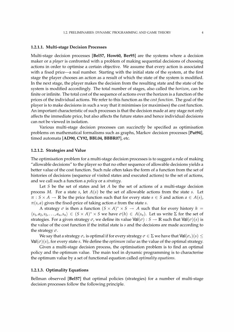
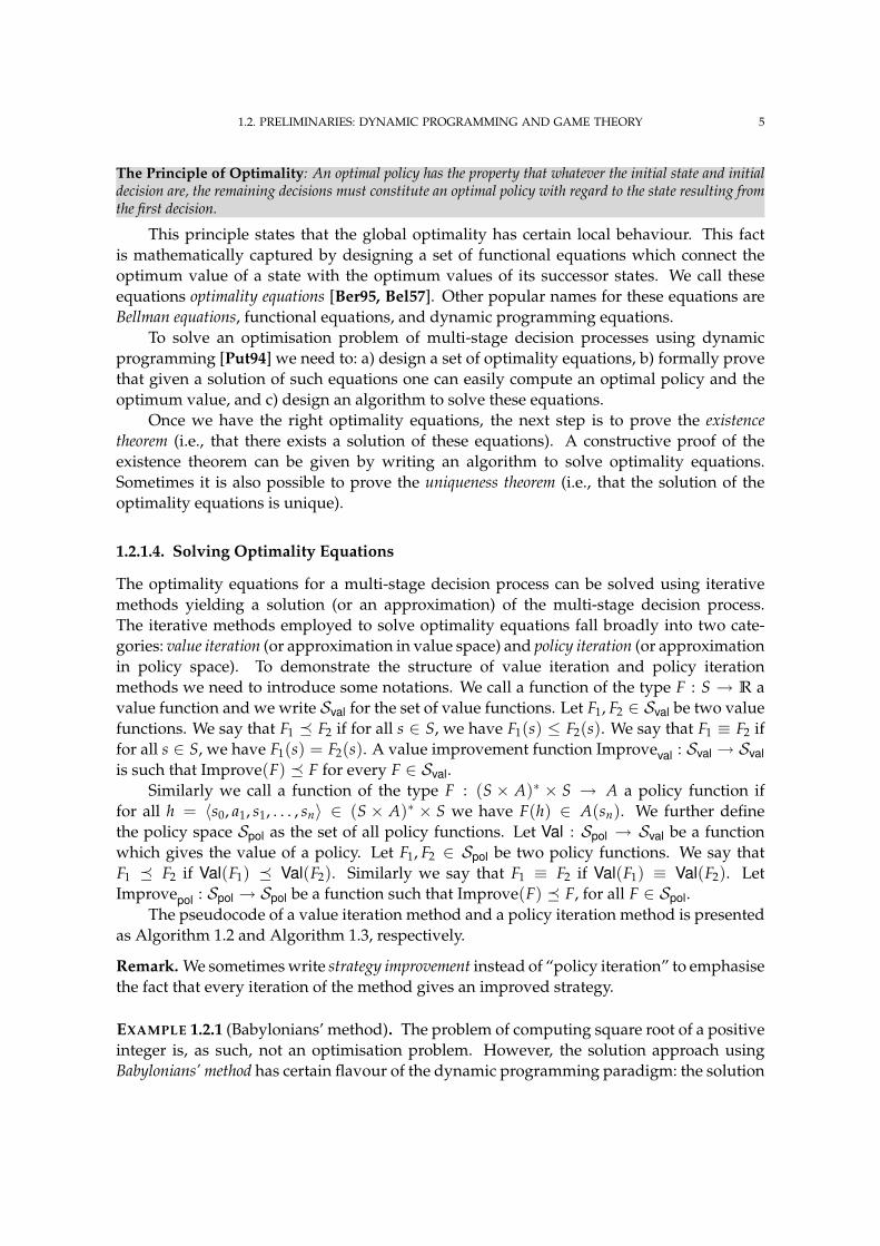
The pseudocode of a value iteration method and a policy iteration method is presentedas Algorithm 1.2 and Algorithm 1.3, respectively.
Remark. We sometimes write strategy improvement instead of “policy iteration” to emphasisethe fact that every iteration of the method gives an improved strategy.
EXAMPLE 1.2.1 (Babylonians’ method). The problem of computing square root of a positiveinteger is, as such, not an optimisation problem. However, the solution approach usingBabylonians’ method has certain flavour of the dynamic programming paradigm: the solution
1.2. PRELIMINARIES: DYNAMIC PROGRAMMING AND GAME THEORY 6
Input: Optimality equationsOutput: A solution of the optimality equationsbegin1
Let V0 ∈ Sval be an arbitrary value function;2
Set i to 0;3
repeat4
Set i := i + 1;5
Vi := Improveval(Vi−1);6
until Vi ≡ Vi−1 ;7
return Vi;8
end9
FIGURE 1.2. Pseudocode of a Value Iteration Method.
Input: Optimality equationsOutput: A solution of the optimality equationsbegin1
Let P0 ∈ Spol be an arbitrary policy;2
Set i to 0;3
repeat4
Set i := i + 1;5
Pi := Improvepol(Pi−1);6
until Pi ≡ Pi−1 ;7
return Val(Pi);8
end9
FIGURE 1.3. Pseudocode of a Policy Iteration Method.
is characterised using equations and then a value iteration algorithm is used to give anapproximation of the solution.
Given a positive integer S ∈ R⊕ we wish to compute its square root to some precisionε > 0. Let us consider the following equation Opt√(S) involving the variable V :
V =12
(V +
SV
).
We say that a number s ∈ [1, ∞) is a solution to Opt√(S), and we write s |= Opt√(S), if theprevious equation holds for the valuation V 7→ s. The following, easy to verify, propositionshows that a solution of this equation gives the positive square root of S.
PROPOSITION 1.2.2. If s ∈ [1, ∞) is such that s |= Opt√(S) then s =√
S.
1.2. PRELIMINARIES: DYNAMIC PROGRAMMING AND GAME THEORY 7
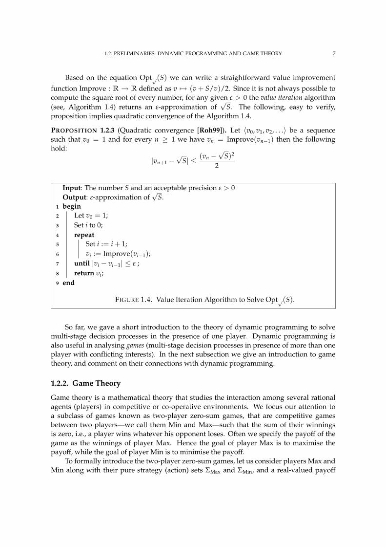
Based on the equation Opt√(S) we can write a straightforward value improvement
function Improve : R → R defined as v 7→ (v + S/v)/2. Since it is not always possible tocompute the square root of every number, for any given ε > 0 the value iteration algorithm(see, Algorithm 1.4) returns an ε-approximation of
√S. The following, easy to verify,
proposition implies quadratic convergence of the Algorithm 1.4.
PROPOSITION 1.2.3 (Quadratic convergence [Roh99]). Let 〈v0, v1, v2, . . .〉 be a sequencesuch that v0 = 1 and for every n ≥ 1 we have vn = Improve(vn−1) then the followinghold:
|vn+1 −√
S| ≤ (vn −√
S)2
2
Input: The number S and an acceptable precision ε > 0Output: ε-approximation of
√S.
begin1
Let v0 = 1;2
Set i to 0;3
repeat4
Set i := i + 1;5
vi := Improve(vi−1);6
until |vi − vi−1| ≤ ε ;7
return vi;8
end9
FIGURE 1.4. Value Iteration Algorithm to Solve Opt√(S).
So far, we gave a short introduction to the theory of dynamic programming to solvemulti-stage decision processes in the presence of one player. Dynamic programming isalso useful in analysing games (multi-stage decision processes in presence of more than oneplayer with conflicting interests). In the next subsection we give an introduction to gametheory, and comment on their connections with dynamic programming.
1.2.2. Game Theory
Game theory is a mathematical theory that studies the interaction among several rationalagents (players) in competitive or co-operative environments. We focus our attention toa subclass of games known as two-player zero-sum games, that are competitive gamesbetween two players—we call them Min and Max—such that the sum of their winningsis zero, i.e., a player wins whatever his opponent loses. Often we specify the payoff of thegame as the winnings of player Max. Hence the goal of player Max is to maximise thepayoff, while the goal of player Min is to minimise the payoff.
To formally introduce the two-player zero-sum games, let us consider players Max andMin along with their pure strategy (action) sets ΣMax and ΣMin, and a real-valued payoff

1.2. PRELIMINARIES: DYNAMIC PROGRAMMING AND GAME THEORY 8
function P : ΣMin × ΣMax → R. If player Max chooses the action χ ∈ ΣMax and playerMin chooses the action µ ∈ ΣMin then we say that the player Max wins the value P(µ, χ)and player Min looses the value P(µ, χ). The goal of player Max is to choose his actions tomaximise his winnings and the goal of the player Min is to choose her actions to minimiseher losses.
Observe that player Max can choose his actions to win at least an amount arbitrarilyclose to supχ∈ΣMax
infµ∈ΣMin P(µ, χ). This is called the lower value Val of the game:
Val= supχ∈ΣMax
infµ∈ΣMin
P(µ, χ). (1.2.1)
Similarly, player Min can choose her actions to lose at most an amount arbitrarily close toinfµ∈ΣMin supχ∈ΣMax
P(µ, χ). This is called the upper value Val of the game:
Val= infµ∈ΣMin
supχ∈ΣMax
P(µ, χ). (1.2.2)
The following proposition states that the lower value is not more than the upper value.
PROPOSITION 1.2.4. For every two-player zero-sum game, it is always the case that Val ≤Val.
PROOF. Observe that for every µ′ ∈ ΣMin and χ′ ∈ ΣMax we have
P(µ′, χ′) ≤ supχ∈ΣMax
P(µ′, χ).
Taking infimum over all strategies of Min we get that for every χ′ ∈ ΣMax we have
infµ∈ΣMin
P(µ, χ′) ≤ infµ∈ΣMin
supχ∈ΣMax
P(µ, χ).
It easily follows that
supχ∈ΣMax
infµ∈ΣMin
P(µ, χ) ≤ infµ∈ΣMin
supχ∈ΣMax
P(µ, χ),
which by definition of Val and Val implies that Val ≤ Val.
We say that a game is determined if Val = Val. If a game is determined then we say thatthe value of the game Val exists and Val = Val = Val.
If the game is determined and the suprema and infima are attained in (1.2.1) and (1.2.2)then optimal strategies χ∗ for player Max and µ∗ player Min are such that the followingholds:
infµ∈ΣMin
P(µ, χ∗) = Val = supχ∈ΣMax
P(µ∗, χ).
However, if Val = Val but the suprema and infima are not attained in (1.2.1) and (1.2.2) thenfor every ε > 0 both players have the so-called ε-optimal strategies. For a given ε > 0, astrategy χε of player Max is called ε-optimal if infµ∈ΣMin P(µ, χε) ≥ Val− ε. Similarly for agiven ε > 0, a strategy µε of player Min is called ε-optimal if supχ∈ΣMax
P(µε, χ) ≤ Val + ε.Observe that not all games are determined. The following example presents a game
that is not determined.
1.3. LITERATURE REVIEW 9
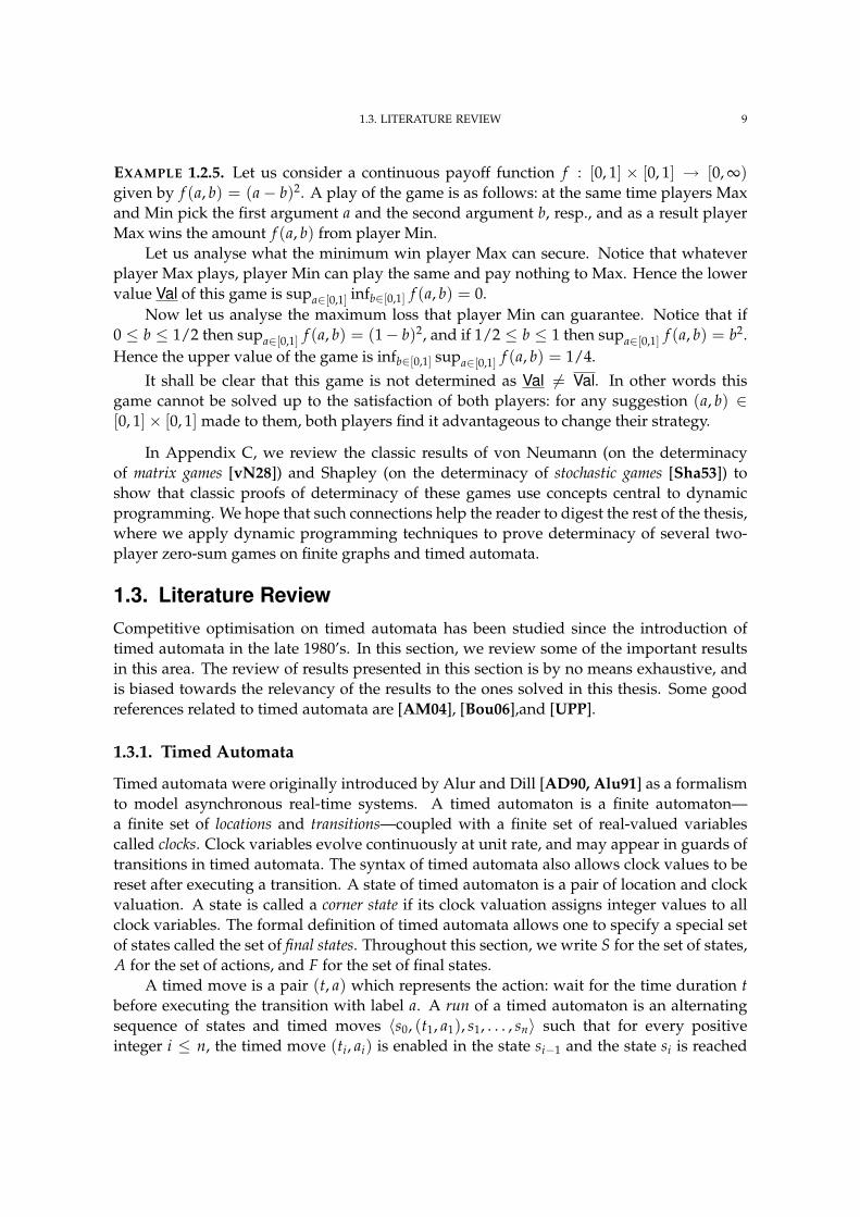
EXAMPLE 1.2.5. Let us consider a continuous payoff function f : [0, 1] × [0, 1] → [0, ∞)given by f (a, b) = (a− b)2. A play of the game is as follows: at the same time players Maxand Min pick the first argument a and the second argument b, resp., and as a result playerMax wins the amount f (a, b) from player Min.
Let us analyse what the minimum win player Max can secure. Notice that whateverplayer Max plays, player Min can play the same and pay nothing to Max. Hence the lowervalue Val of this game is supa∈[0,1] infb∈[0,1] f (a, b) = 0.
Now let us analyse the maximum loss that player Min can guarantee. Notice that if0 ≤ b ≤ 1/2 then supa∈[0,1] f (a, b) = (1− b)2, and if 1/2 ≤ b ≤ 1 then supa∈[0,1] f (a, b) = b2.Hence the upper value of the game is infb∈[0,1] supa∈[0,1] f (a, b) = 1/4.
It shall be clear that this game is not determined as Val 6= Val. In other words thisgame cannot be solved up to the satisfaction of both players: for any suggestion (a, b) ∈[0, 1]× [0, 1] made to them, both players find it advantageous to change their strategy.
In Appendix C, we review the classic results of von Neumann (on the determinacyof matrix games [vN28]) and Shapley (on the determinacy of stochastic games [Sha53]) toshow that classic proofs of determinacy of these games use concepts central to dynamicprogramming. We hope that such connections help the reader to digest the rest of the thesis,where we apply dynamic programming techniques to prove determinacy of several two-player zero-sum games on finite graphs and timed automata.
1.3. Literature ReviewCompetitive optimisation on timed automata has been studied since the introduction oftimed automata in the late 1980’s. In this section, we review some of the important resultsin this area. The review of results presented in this section is by no means exhaustive, andis biased towards the relevancy of the results to the ones solved in this thesis. Some goodreferences related to timed automata are [AM04], [Bou06],and [UPP].
1.3.1. Timed Automata
Timed automata were originally introduced by Alur and Dill [AD90, Alu91] as a formalismto model asynchronous real-time systems. A timed automaton is a finite automaton—a finite set of locations and transitions—coupled with a finite set of real-valued variablescalled clocks. Clock variables evolve continuously at unit rate, and may appear in guards oftransitions in timed automata. The syntax of timed automata also allows clock values to bereset after executing a transition. A state of timed automaton is a pair of location and clockvaluation. A state is called a corner state if its clock valuation assigns integer values to allclock variables. The formal definition of timed automata allows one to specify a special setof states called the set of final states. Throughout this section, we write S for the set of states,A for the set of actions, and F for the set of final states.
A timed move is a pair (t, a) which represents the action: wait for the time duration tbefore executing the transition with label a. A run of a timed automaton is an alternatingsequence of states and timed moves 〈s0, (t1, a1), s1, . . . , sn〉 such that for every positiveinteger i ≤ n, the timed move (ti, ai) is enabled in the state si−1 and the state si is reached
1.3. LITERATURE REVIEW 10
after executing the timed move (ti, ai). An infinite run r = 〈s0, (t1, a1), . . .〉 is definedanalogously. We say that a run 〈s0, (t1, a1), s1, . . . , sn〉 is accepting if the state sn ∈ F. Thelanguage recognised by a timed automaton is the set of accepting runs. In their seminalpaper, Alur and Dill [AD90] showed that languages recognised by timed automata areclosed under union and intersection, but not under complementation.
1.3.2. Noncompetitive Optimisation Problems
1.3.2.1. Reachability Problem
The reachability problem of a timed automaton is: given an initial state s ∈ S, decide whethera final state is reachable from the initial state, i.e., whether there exists an accepting runstarting from s.
Alur and Dill [AD90] showed that the reachability problem for timed automata isdecidable and that it is PSPACE-complete. They established PSPACE-membership of thereachability problem using a finitary abstraction—the so-called region graph—of timedautomata, whose size is exponential in the size of the timed automaton. For the PSPACE-hardness result they showed that for a linear-space Turing machine M and an input wordw of length n, there exists a timed automaton T with 2n + 1 clocks, such that the languageof T is nonempty iff the machine M accepts w. Courcoubetis and Yannakakis [CY92] latertightened the PSPACE-hardness result by showing a reduction from the acceptance problemfor linear-space Turing machine to the reachability problem of timed automata with onlythree clocks.
THEOREM 1.3.1 ([AD94, CY92]). The reachability problem is PSPACE-complete for timedautomata with at least three clocks.
Laroussinie, Markey and Schnoebelen [LMS04] proposed a succinct “region” graphabstraction for one-clock timed automata, and using that they proved that the reachabilityproblem for one-clock timed automata is NLOGSPACE-complete.
THEOREM 1.3.2 ([LMS04]). The reachability problem is NLOGSPACE-complete for timedautomata with one clock.
The exact complexity of the reachability problem for timed automata with two clocksremains an open question.
1.3.2.2. Optimal Reachability-Time Problem
A natural optimisation problem on the timed automata is to optimise (minimise ormaximise) reachability time, i.e., total time to reach a final state. Given a timed automatonT , an initial state s, and a number D ∈ R⊕, the minimum reachability time problem isto decide whether there exists an accepting run starting from s with total time at most D.Maximum reachability-time problem is defined analogously.
Minimum and maximum reachability-time problems were shown to be decidable byCourcoubetis and Yannakakis [CY92]. It was shown to be PSPACE-complete by Alur,Courcoubetis, and Henzinger [ACH97] and Kesten et al. [KPSS99]. An efficient algorithm
1.3. LITERATURE REVIEW 11
to solve the minimum reachability-time problem on timed automata appeared in [NTY00],where the initial state was restricted to corner states.
1.3.2.3. Optimal Reachability-Price Problem
A generalisation of timed automata to priced timed automata [Bou06]—also known asweighted timed automata—allows a rich variety of applications, e.g., to optimal schedul-ing [BFH+01, AM01]. Priced timed automata are timed automata with a price functionπ : S × R⊕ × A → R such that π(s, (t, a)) gives the price of taking a timed move (t, a)from a state s. The price function can be extended to give the reachability-price RP(r) of aninfinite run r = 〈s0, (t1, a1), s1, . . .〉, the sum of the prices of the timed moves before reachinga final state, in the following manner:
RP(r) =
∑Stop(r)
i=1 π(si−1, (ti, ai)), if Stop(r) < +∞,
∞, otherwise,
where Stop(r) denotes the index of the first final state in the run r.Linearly-priced timed automata, a sub-class of priced timed automata, augment the
timed automata with price information, such that the price of waiting in a state is directlyproportional to the waiting time. A natural generalisation of the minimum reachability-timeproblem for the timed automata is the minimum reachability-price problem for the pricedtimed automata.
Given a priced timed automaton T , an initial state s, and a number D, the minimumreachability-price problem is to decide whether there exists an infinite run r starting from ssuch that RP(r) ≤ D.
For a linearly-priced timed automaton, Larsen et al. [LBB+01, BFH+01, LBB+04] pro-posed symbolic algorithms to solve the reachability-price problem, with some restrictionson the initial state (corner state with all clocks set to zero). These symbolic algorithms arealso implemented as a part of UPPAAL [BFHL01] (a toolkit for the verification of real-timesystems).
In [ALTP04] Alur et al. proposed an EXPTIME algorithm to solve the reachability-price problem for linearly-priced timed automata using a non-trivial extension of the regiongraph.
Bouyer et al. [BBBR07] showed that the reachability-price problem for the linearly-priced timed automata is PSPACE-complete, given the initial state is a corner state. ThePSPACE-hardness result for this problem comes from a straightforward reduction fromthe reachability problem for timed automata. To show PSPACE-membership, Bouyer etal. argued that the minimum reachability-price for a linearly-priced timed automaton canbe computed using a finitary abstraction of the timed automata, if the initial state is acorner state. The abstraction used by them is called the corner-point abstraction. Theirmain observation was that if the initial state is a corner state, then optimal (nearly optimal)reachability-price runs go through (or very close to) corner states.
Remark. Notice that PSPACE-completeness result of Bouyer et al. [BBBR07] for theoptimum reachability-price problem is restricted to linearly-priced timed automata andinitial states that are corner states.
1.3. LITERATURE REVIEW 12
Observe that PSPACE-completeness results, for reachability-time and reachability-priceproblems, hold for timed automata with at least three clocks. For timed automata withone clock, reachability-time and reachability-price problems are known to be NLOGSPACE-complete [LMS04]; while the complexity of these problems for two-clock timed automataremains an open problem.
1.3.2.4. Optimal Average-Price Problem
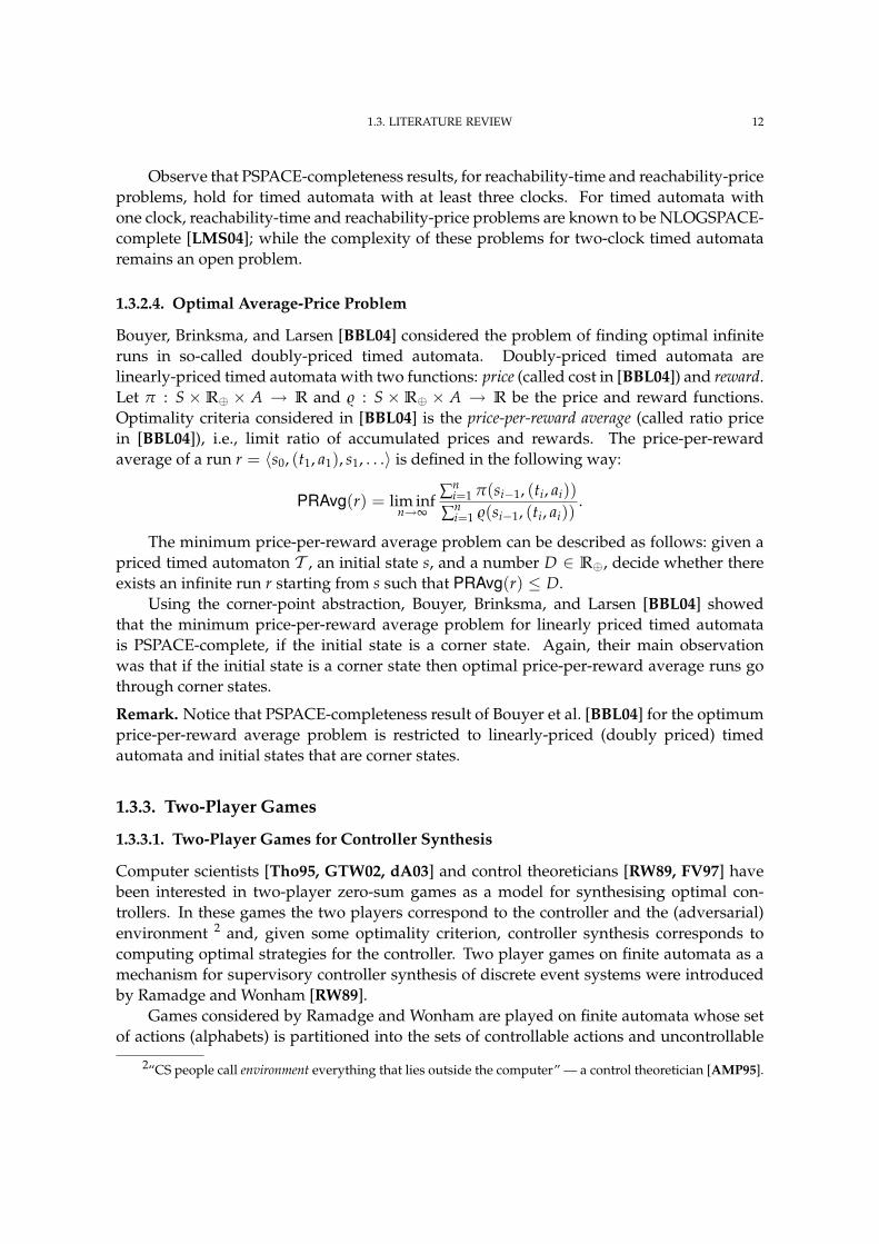
Bouyer, Brinksma, and Larsen [BBL04] considered the problem of finding optimal infiniteruns in so-called doubly-priced timed automata. Doubly-priced timed automata arelinearly-priced timed automata with two functions: price (called cost in [BBL04]) and reward.Let π : S ×R⊕ × A → R and $ : S ×R⊕ × A → R be the price and reward functions.Optimality criteria considered in [BBL04] is the price-per-reward average (called ratio pricein [BBL04]), i.e., limit ratio of accumulated prices and rewards. The price-per-rewardaverage of a run r = 〈s0, (t1, a1), s1, . . .〉 is defined in the following way:
PRAvg(r) = lim infn→∞
∑ni=1 π(si−1, (ti, ai))
∑ni=1 $(si−1, (ti, ai))
.
The minimum price-per-reward average problem can be described as follows: given apriced timed automaton T , an initial state s, and a number D ∈ R⊕, decide whether thereexists an infinite run r starting from s such that PRAvg(r) ≤ D.
Using the corner-point abstraction, Bouyer, Brinksma, and Larsen [BBL04] showedthat the minimum price-per-reward average problem for linearly priced timed automatais PSPACE-complete, if the initial state is a corner state. Again, their main observationwas that if the initial state is a corner state then optimal price-per-reward average runs gothrough corner states.
Remark. Notice that PSPACE-completeness result of Bouyer et al. [BBL04] for the optimumprice-per-reward average problem is restricted to linearly-priced (doubly priced) timedautomata and initial states that are corner states.
1.3.3. Two-Player Games
1.3.3.1. Two-Player Games for Controller Synthesis
Computer scientists [Tho95, GTW02, dA03] and control theoreticians [RW89, FV97] havebeen interested in two-player zero-sum games as a model for synthesising optimal con-trollers. In these games the two players correspond to the controller and the (adversarial)environment 2 and, given some optimality criterion, controller synthesis corresponds tocomputing optimal strategies for the controller. Two player games on finite automata as amechanism for supervisory controller synthesis of discrete event systems were introducedby Ramadge and Wonham [RW89].
Games considered by Ramadge and Wonham are played on finite automata whose setof actions (alphabets) is partitioned into the sets of controllable actions and uncontrollable
2“CS people call environment everything that lies outside the computer” — a control theoretician [AMP95].
1.3. LITERATURE REVIEW 13
actions. The objective considered by them is safety (or equivalently reachability), i.e., “toavoid bad states”. A strategy of the controller is a function from the set of runs to the setof controllable actions, which—based on the history of the run—suggests the controller toselect a controllable event in order to optimise the objective, i.e., to avoid reaching a badstate. The solution proposed by Ramadge and Wonham is based on computing greatestfixed point of certain controllable predecessor functions.
1.3.3.2. Reachability Games
Hoffman and Wong-Toi [WTH92, HWT92] were the first ones to define and solve optimalcontroller synthesis problem for timed automata. They proved the decidability of reacha-bility games on timed automata by extending the method of Ramadge and Wonham to thefinitary region graph abstraction of timed automata.
Asarin, Maler and Pnueli [AMP95] give a symbolic algorithm for optimal controllersynthesis of timed automata. Their work is closely related to the work by Hoffman andWong-Toi. However, instead of explicitly constructing the region graph, they use symbolicmethods, representing the set of states using arbitrary linear inequalities, to solve thereachability game on timed automata.
Henzinger and Kopke [HK99] show that the complexity of solving reachability gameson timed automata is EXPTIME-complete. Jurdzinski and I [JT07] improved their results byshowing that reachability games are EXPTIME-complete for timed automata with at leasttwo clocks.
For a detailed introduction to the topic of qualitative games on timed automata, werecommend papers by Asarin et al. [AMPS98, AMP95].
1.3.3.3. Reachability-Time Games
Asarin and Maler [AM99] initiated the study of quantitative competitive optimisationon timed automata. They considered reachability-time games where controller (playerMin in our terminology) is interested in reaching a final state as soon as possible. Thesymbolic algorithm presented in [AM99] is a value iteration algorithm, which solves a set ofoptimality equations characterising minimum time to reach a final state. They give a uniformsolution, i.e., their algorithm computes a function which, given an initial state, returns theupper-value of the reachability-time game starting from that state. The result of Asarinand Maler does not give any upper complexity bounds and is restricted to a subclass: thestructurally non-Zeno timed automata.
Brihaye et al. [BHPR07] and Jurdzinski and I [JT07] studied reachability-time gamesfor slightly different models of timed games, and showed that the decision version of thereachability-time game is EXPTIME-complete for timed automata with at least two clocks.
Brihaye et al. [BHPR07] studied the problem on the “element-of-surprise” timed gamemodel introduced in [dAFH+03]. In these models players can take each other by surpriseas both players suggest a timed move concurrently, and the timed move with shorter timedelay is executed. They also introduced a nice concept of a receptive strategy—a strategywhich does not recommend players to execute infinitely many actions in a finite amount
1.3. LITERATURE REVIEW 14
of time—and to win a game a player must use a receptive strategy. Analysis using onlyreceptive strategies is arguably more meaningful, because strategies of the controller thatare not receptive are not physically implementable. Unfortunately, receptiveness is not asufficient condition for a strategy to be implementable, e.g., consider the strategy in whichcontroller needs to act in the following time sequence: 〈0, 1
2 , 1, 1 14 , 2, 2 1
8 , 3, 3 116 , . . .〉 [CHR02].
Moreover, reachability-time games studied by Brihaye et al. are not known to be determinedand they compute the upper value of the game.
Jurdzinski and I [JT07] studied a turn-based model of timed games where the locationsof the timed automata are partitioned between two players. For these models of timedgame, we proved that reachability-time games are positionally determined. Our algorithmgives a uniform solution, and by analysing our algorithm we show that reachability-timegames are EXPTIME-complete for timed automata with at least two clocks. However, unlikeBrihaye et al. [BHPR07], we do not require players to play only receptive strategies.
1.3.3.4. Rechability-Price Games
A natural extension of reachability-time games for timed automata is reachability-pricegames for priced timed automata.
La Torre, Mukhopadhyay, and Murano [LTMM02] studied reachability-price games ona restricted class, the so-called acyclic timed automata, of linearly-priced timed automata.They gave a doubly-exponential time algorithm to solve the reachability-price games ontimed automata, given that the timed automaton is acyclic, i.e., control graph does not haveany cycles.
Alur, Bernadsky, and Madhusudan [ABM04] and Bouyer et al. [BCFL04] studied,independently, the reachability-price games on arbitrary linearly-priced priced timedautomata, and gave semi-algorithms to compute its upper value of the reachability-pricegames. Their algorithms are guaranteed to terminate for linearly-priced timed automatawith non-Zeno prices, i.e., every cycle of the automaton has a bounded positive price.The elegant paper of Alur et al. [ABM04] presents a value-iteration algorithm to uniformlycompute the upper value of a reachability-price game. The authors also present a detailedunderstanding of the value iteration method in which, at every iteration, the regions aresplit into sub-regions such that the approximation of the upper value in a sub-regionis a linear function. Alur et al. also showed that for certain examples regions get splitinto exponentially many such sub-regions. The solution of Bouyer et al. [BCFL04], onthe other hand, is based on a reduction to games on linear hybrid automata. They alsopresented [BCFL05] techniques to implement the solution using the HyTech tool.
Brihaye, Bruyere, and Raskin [BBR05] proved a somewhat unexpected result thatchecking the existence of optimal strategies in a reachability-price game is undecidablefor a priced timed automaton with at least five clocks. They showed a reduction fromthe halting problem for two-counter machines to the problem of finding reachability-priceoptimal strategies in priced timed automata with five clocks and with stopwatch prices (i.e.,with either 0 or 1 price rates of the locations).
Bouyer, Brihaye, and Markey [BBM06] later improved this undecidability result byreducing the halting problem for two-counter machine to finding optimal strategies in a
1.4. CONTRIBUTIONS OF THE THESIS 15
reachability-price game on a priced timed automaton with three clocks and with stopwatchprices. The problem of finding reachability-price optimal strategies for linearly-priced timedautomata with one clock is known to be decidable, and Bouyer et al. [BLMR06] give a3EXPTIME algorithm to solve this problem. The decidability of finding optimal strategiesin a reachability-price game on timed automata with two clocks is unknown.
Finally, notice that the decidability of finding the value of a state in a reachability-pricegame remains an open problem.
1.4. Contributions of the Thesis1.4.1. Boundary Strategies and Boundary Region Graphs
We view a competitive optimisation problem on timed automata as a multi-stage decisionprocess where one or two players are confronted with the problem of choosing a sequenceof timed moves—each consisting of a time delay and an action—in order to optimise theirobjectives given as a cost function. A solution of such problems consists of the “optimum”value of the cost function and an “optimal” strategy for each player. We highlight a usefulclass of strategies, called boundary strategies, that suggest to a player a symbolic timed moveof the form (b, c, a)— “wait until the value of the clock c is in very close proximity of theinteger b, and then execute a transition labelled with the action a”. A distinctive feature ofthe competitive optimisation problems discussed in this thesis is the existence of optimalboundary strategies.
The existence of optimal boundary strategies allows us to work with a novel abstractionof the timed automata, called a boundary region graph, where players can use only boundarystrategies. An important property of a boundary region graph is that for every state theset of reachable states is finite (exponential in the size of the timed automaton). Hence,the existence of optimal boundary strategies allows us to reduce a competitive optimisationproblem on a timed automaton to the corresponding competitive optimisation problem ona finite graph.
Boundary region graphs generalise corner-point abstractions of timed automata in-troduced by Bouyer et al. Corner-point abstractions are useful in analysing variousoptimisation problems on timed automata, given that the initial state is a corner-state (astate with integral valuation to every clock). On the other hand, our boundary region graphpermits the analysis of a number of competitive optimisation problems on timed automatawith arbitrary initial states, including non-corner states.
1.4.2. Non-competitive Optimisation
To cover a large class of optimisation problems we introduce concavely-priced timed automata,that are generalisations of timed automata with price information given by certain concavefunctions. We identify a useful property, called concave-regularity, of the cost function: ifa cost function is concave-regular then there exists an optimal boundary strategy for thecorresponding optimisation problem. We show that a number of cost functions of practicalinterest, including reachability price, discounted price, average time-per-transition, averageprice-per-transition, and average price-per-time-unit, are concave-regular. We further show
1.4. CONTRIBUTIONS OF THE THESIS 16
that the complexity of solving optimisation problems for concave-regular cost functions isPSPACE-complete on timed automata with three or more clocks.
THEOREM. The minimisation problems for reachability price, discounted price, averageprice, price-per-time average, and price-per-reward average cost functions, for concavely-priced and concave price-reward timed automata, as appropriate, are PSPACE-complete.
We generalise some previously known complexity results (e.g., the results of Bouyer etal. on optimum reachability price problem [BBBR07] and on optimum price-per-rewardaverage problem[BBL04]) in two directions: a) our results are valid for arbitrary initialstates, and b) we consider more general concavely-priced timed automata.
1.4.3. Reachability-Time Games
A reachability-time game is played between two players Min and Max on the infinitegraph of configurations of a timed automaton. The goals of player Min and player Maxare to minimise and maximise, respectively, the time to reach a designated set of finalconfigurations. We show that the exact values of reachability-time games on arbitrarytimed automata are uniformly computable (here uniformity means that the output of ouralgorithm allows us, for every starting state, to compute in constant time the value of thegame starting from this state). In particular, unlike the paper of Asarin and Maler [AM99],we do not require timed automata to be strongly non-Zeno. We also establish the exactcomplexity of reachability-time games: they are EXPTIME-complete and two clocks aresufficient for EXPTIME-hardness. For the latter result, we reduce from a recently discoveredEXPTIME-complete problem of countdown games [JLS07].
THEOREM. The problem of solving reachability-time games is EXPTIME-complete ontimed automata with at least two clocks.
We believe that an important contribution of our work on reachability-time games is thenovel proof techniques used. We characterise the values of the game by optimality equationsand then we use strategy improvement to solve them. This allows us to obtain an elementaryand constructive proof of the fundamental determinacy result for reachability-time games,which at the same time yields an efficient algorithm matching the EXPTIME lower boundfor the problem. Those techniques were known for finite state systems [Put94, VJ00], but weare not aware of any earlier algorithmic results based on optimality equations and strategyimprovement for real-time systems such as timed automata.
1.4.4. Average-Time Games
An average time game is played on the infinite graph of configurations of a finite timedautomaton. The two players, Min and Max, construct an infinite run of the automaton bytaking turns to perform a timed transition. Player Min wants to minimise the average timeper transition and player Max wants to maximise it. We give a solution of the average-time games using a reduction to the average-price game on the finite graph of reachableconfigurations of the boundary region graph. A direct consequence is an elementary
1.5. ORGANISATION OF THE THESIS 17
proof of determinacy for average-time games. Our solution allows computing the valueof average-time games for an arbitrary starting state (i.e., including non-corner states). Wealso establish the exact complexity of average-time games: they are EXPTIME-complete andtwo clocks are sufficient for EXPTIME-hardness. For the hardness result we reduce fromEXPTIME-complete problem of countdown games [JLS07].
THEOREM. The problem of solving average-time games is EXPTIME-complete on timedautomata with at least two clocks.
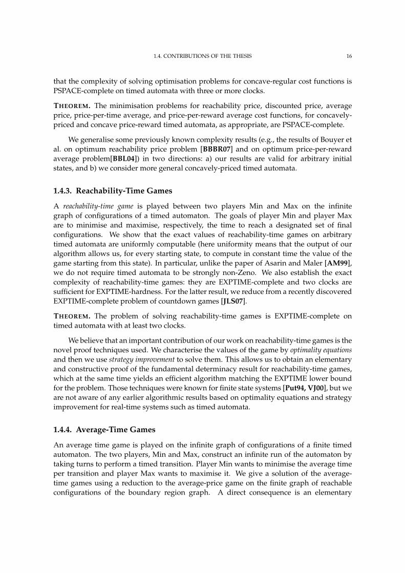
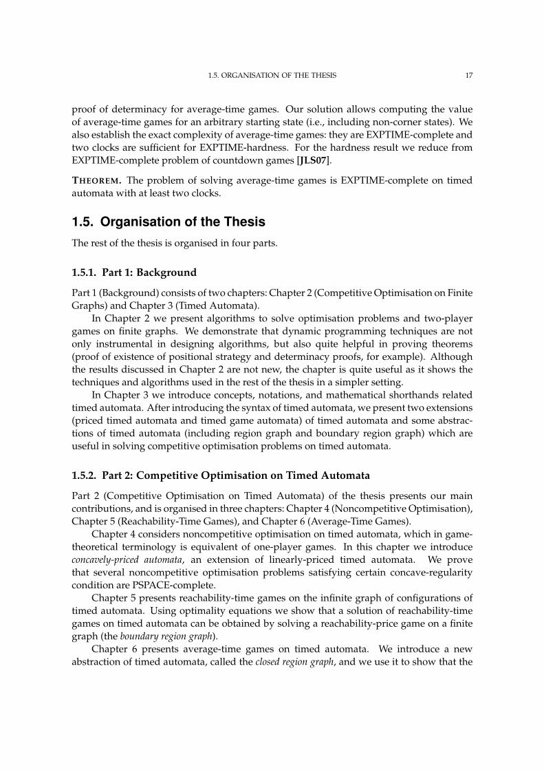
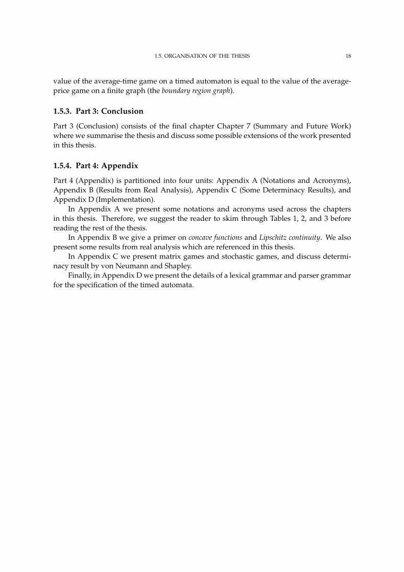
1.5. Organisation of the ThesisThe rest of the thesis is organised in four parts.
1.5.1. Part 1: Background
Part 1 (Background) consists of two chapters: Chapter 2 (Competitive Optimisation on FiniteGraphs) and Chapter 3 (Timed Automata).
In Chapter 2 we present algorithms to solve optimisation problems and two-playergames on finite graphs. We demonstrate that dynamic programming techniques are notonly instrumental in designing algorithms, but also quite helpful in proving theorems(proof of existence of positional strategy and determinacy proofs, for example). Althoughthe results discussed in Chapter 2 are not new, the chapter is quite useful as it shows thetechniques and algorithms used in the rest of the thesis in a simpler setting.
In Chapter 3 we introduce concepts, notations, and mathematical shorthands relatedtimed automata. After introducing the syntax of timed automata, we present two extensions(priced timed automata and timed game automata) of timed automata and some abstrac-tions of timed automata (including region graph and boundary region graph) which areuseful in solving competitive optimisation problems on timed automata.
1.5.2. Part 2: Competitive Optimisation on Timed Automata
Part 2 (Competitive Optimisation on Timed Automata) of the thesis presents our maincontributions, and is organised in three chapters: Chapter 4 (Noncompetitive Optimisation),Chapter 5 (Reachability-Time Games), and Chapter 6 (Average-Time Games).
Chapter 4 considers noncompetitive optimisation on timed automata, which in game-theoretical terminology is equivalent of one-player games. In this chapter we introduceconcavely-priced automata, an extension of linearly-priced timed automata. We provethat several noncompetitive optimisation problems satisfying certain concave-regularitycondition are PSPACE-complete.
Chapter 5 presents reachability-time games on the infinite graph of configurations oftimed automata. Using optimality equations we show that a solution of reachability-timegames on timed automata can be obtained by solving a reachability-price game on a finitegraph (the boundary region graph).
Chapter 6 presents average-time games on timed automata. We introduce a newabstraction of timed automata, called the closed region graph, and we use it to show that the
1.5. ORGANISATION OF THE THESIS 18
value of the average-time game on a timed automaton is equal to the value of the average-price game on a finite graph (the boundary region graph).
1.5.3. Part 3: Conclusion
Part 3 (Conclusion) consists of the final chapter Chapter 7 (Summary and Future Work)where we summarise the thesis and discuss some possible extensions of the work presentedin this thesis.
1.5.4. Part 4: Appendix
Part 4 (Appendix) is partitioned into four units: Appendix A (Notations and Acronyms),Appendix B (Results from Real Analysis), Appendix C (Some Determinacy Results), andAppendix D (Implementation).
In Appendix A we present some notations and acronyms used across the chaptersin this thesis. Therefore, we suggest the reader to skim through Tables 1, 2, and 3 beforereading the rest of the thesis.
In Appendix B we give a primer on concave functions and Lipschitz continuity. We alsopresent some results from real analysis which are referenced in this thesis.
In Appendix C we present matrix games and stochastic games, and discuss determi-nacy result by von Neumann and Shapley.
Finally, in Appendix D we present the details of a lexical grammar and parser grammarfor the specification of the timed automata.
Part 1
Background
2Competitive Optimisation onFinite Graphs
If you keep proving stuff thatothers have done, gettingconfidence, increasing thecomplexities of your solutions -for the fun of it - then one dayyou’ll turn around and discoverthat nobody actually did thatone! And that’s the way tobecome a computer scientist.
Richard Feynmann
In this chapter we provide an introduction to competitive optimisation on finitegraphs 1. We discuss optimisation problems and two-player games on finite graphs, andpresent dynamic programming based algorithms to solve them. Competitive optimisationfor the following cost functions are discussed: reachability price, discounted price, averageprice, and price-per-reward average. This chapter lays the foundations that are essential inthe development of algorithms to solve competitive optimisation problems on the infinitegraph of configurations of timed automata.
2.1. Formal DefinitionDEFINITION 2.1.1 (Finite Graph). A (directed) finite graph is a pair G = (V, E), where:
– V is a finite set whose elements are called vertices, and– E ⊆ V ×V is a set of ordered pairs of vertices whose elements are called (directed)
edges.
1 Disclaimer: the concepts, theorems, and their proofs presented in this chapter are standard. Similartreatment can be found in an advanced setting of Markov Decision Processes in the excellent books ofPuterman [Put94], and Filar and Vrieze [FV97].
20
2.1. FORMAL DEFINITION 21
v1v2 v3
20
0
0
0
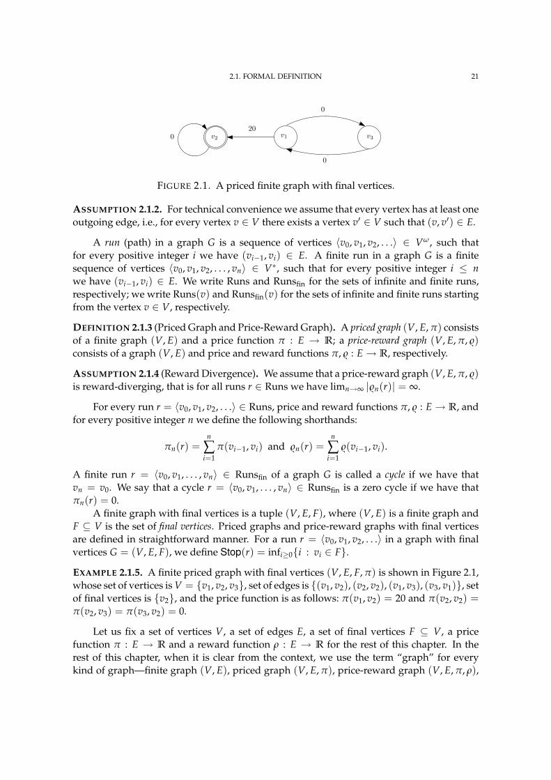
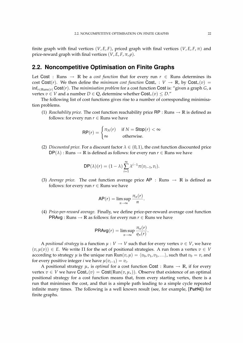
FIGURE 2.1. A priced finite graph with final vertices.
ASSUMPTION 2.1.2. For technical convenience we assume that every vertex has at least oneoutgoing edge, i.e., for every vertex v ∈ V there exists a vertex v′ ∈ V such that (v, v′) ∈ E.
A run (path) in a graph G is a sequence of vertices 〈v0, v1, v2, . . .〉 ∈ Vω, such thatfor every positive integer i we have (vi−1, vi) ∈ E. A finite run in a graph G is a finitesequence of vertices 〈v0, v1, v2, . . . , vn〉 ∈ V∗, such that for every positive integer i ≤ nwe have (vi−1, vi) ∈ E. We write Runs and Runsfin for the sets of infinite and finite runs,respectively; we write Runs(v) and Runsfin(v) for the sets of infinite and finite runs startingfrom the vertex v ∈ V, respectively.
DEFINITION 2.1.3 (Priced Graph and Price-Reward Graph). A priced graph (V, E, π) consistsof a finite graph (V, E) and a price function π : E → R; a price-reward graph (V, E, π, $)consists of a graph (V, E) and price and reward functions π, $ : E→ R, respectively.
ASSUMPTION 2.1.4 (Reward Divergence). We assume that a price-reward graph (V, E, π, $)is reward-diverging, that is for all runs r ∈ Runs we have limn→∞ |$n(r)| = ∞.
For every run r = 〈v0, v1, v2, . . .〉 ∈ Runs, price and reward functions π, $ : E→ R, andfor every positive integer n we define the following shorthands:
πn(r) =n
∑i=1
π(vi−1, vi) and $n(r) =n
∑i=1
$(vi−1, vi).
A finite run r = 〈v0, v1, . . . , vn〉 ∈ Runsfin of a graph G is called a cycle if we have thatvn = v0. We say that a cycle r = 〈v0, v1, . . . , vn〉 ∈ Runsfin is a zero cycle if we have thatπn(r) = 0.
A finite graph with final vertices is a tuple (V, E, F), where (V, E) is a finite graph andF ⊆ V is the set of final vertices. Priced graphs and price-reward graphs with final verticesare defined in straightforward manner. For a run r = 〈v0, v1, v2, . . .〉 in a graph with finalvertices G = (V, E, F), we define Stop(r) = infi≥0i : vi ∈ F.EXAMPLE 2.1.5. A finite priced graph with final vertices (V, E, F, π) is shown in Figure 2.1,whose set of vertices is V = v1, v2, v3, set of edges is (v1, v2), (v2, v2), (v1, v3), (v3, v1), setof final vertices is v2, and the price function is as follows: π(v1, v2) = 20 and π(v2, v2) =π(v2, v3) = π(v3, v2) = 0.
Let us fix a set of vertices V, a set of edges E, a set of final vertices F ⊆ V, a pricefunction π : E → R and a reward function ρ : E → R for the rest of this chapter. In therest of this chapter, when it is clear from the context, we use the term “graph” for everykind of graph—finite graph (V, E), priced graph (V, E, π), price-reward graph (V, E, π, ρ),
2.2. NONCOMPETITIVE OPTIMISATION ON FINITE GRAPHS 22
finite graph with final vertices (V, E, F), priced graph with final vertices (V, E, F, π) andprice-reward graph with final vertices (V, E, F, π, ρ).
2.2. Noncompetitive Optimisation on Finite GraphsLet Cost : Runs → R be a cost function that for every run r ∈ Runs determines itscost Cost(r). We then define the minimum cost function Cost∗ : V → R, by Cost∗(v) =infr∈Runs(v) Cost(r). The minimisation problem for a cost function Cost is: “given a graph G, avertex v ∈ V and a number D ∈ Q, determine whether Cost∗(v) ≤ D.”
The following list of cost functions gives rise to a number of corresponding minimisa-tion problems.
(1) Reachability price. The cost function reachability price RP : Runs→ R is defined asfollows: for every run r ∈ Runs we have
RP(r) =
πN(r) if N = Stop(r) < ∞∞ otherwise.
(2) Discounted price. For a discount factor λ ∈ (0, 1), the cost function discounted priceDP(λ) : Runs→ R is defined as follows: for every run r ∈ Runs we have
DP(λ)(r) = (1− λ)∞
∑i=1
λi−1π(vi−1, vi).
(3) Average price. The cost function average price AP : Runs → R is defined asfollows: for every run r ∈ Runs we have
AP(r) = lim supn→∞
πn(r)n
.
(4) Price-per-reward average. Finally, we define price-per-reward average cost functionPRAvg : Runs→ R as follows: for every run r ∈ Runs we have
PRAvg(r) = lim supn→∞
πn(r)$n(r)
.
A positional strategy is a function µ : V → V such that for every vertex v ∈ V, we have(v, µ(v)) ∈ E. We write Π for the set of positional strategies. A run from a vertex v ∈ Vaccording to strategy µ is the unique run Run(v, µ) = 〈v0, v1, v2, . . .〉, such that v0 = v, andfor every positive integer i we have µ(vi−1) = vi.
A positional strategy µ∗ is optimal for a cost function Cost : Runs → R, if for everyvertex v ∈ V we have Cost∗(v) = Cost(Run(v, µ∗)). Observe that existence of an optimalpositional strategy for a cost function means that, from every starting vertex, there is arun that minimises the cost, and that is a simple path leading to a simple cycle repeatedinfinite many times. The following is a well known result (see, for example, [Put94]) forfinite graphs.
2.2. NONCOMPETITIVE OPTIMISATION ON FINITE GRAPHS 23
THEOREM 2.2.1 (Existence of optimal positional strategies). For every finite graph, andfor each of the reachability, discounted, average price, and price-per-reward average costfunctions, there is an optimal positional strategy.
The rest of this section is devoted to the proof of this theorem. For each of the costfunctions defined above, we design a set of optimality equations such that the existence ofa solution of those equations implies the existence of a positional strategy. A solution ofoptimality equations also characterises the minimum cost function. We give a constructiveproof of the existence of a solution by giving a strategy improvement algorithm, whichreturns a solution of the optimality equations.
2.2.1. Solving Reachability-Price Minimisation Problem
2.2.1.1. Optimality Equations
Let G = (V, E, F, π) be a finite graph with final vertices. To keep the discussion simple, weassume that the graph G satisfy the following assumption:
ASSUMPTION 2.2.2. For every vertex v ∈ V we have that minimum reachability-price isfinite.
Before we consider the problem in full generality, we try to solve a simpler problemand assume the following:
ASSUMPTION 2.2.3. The graph G does not have any zero cycles.
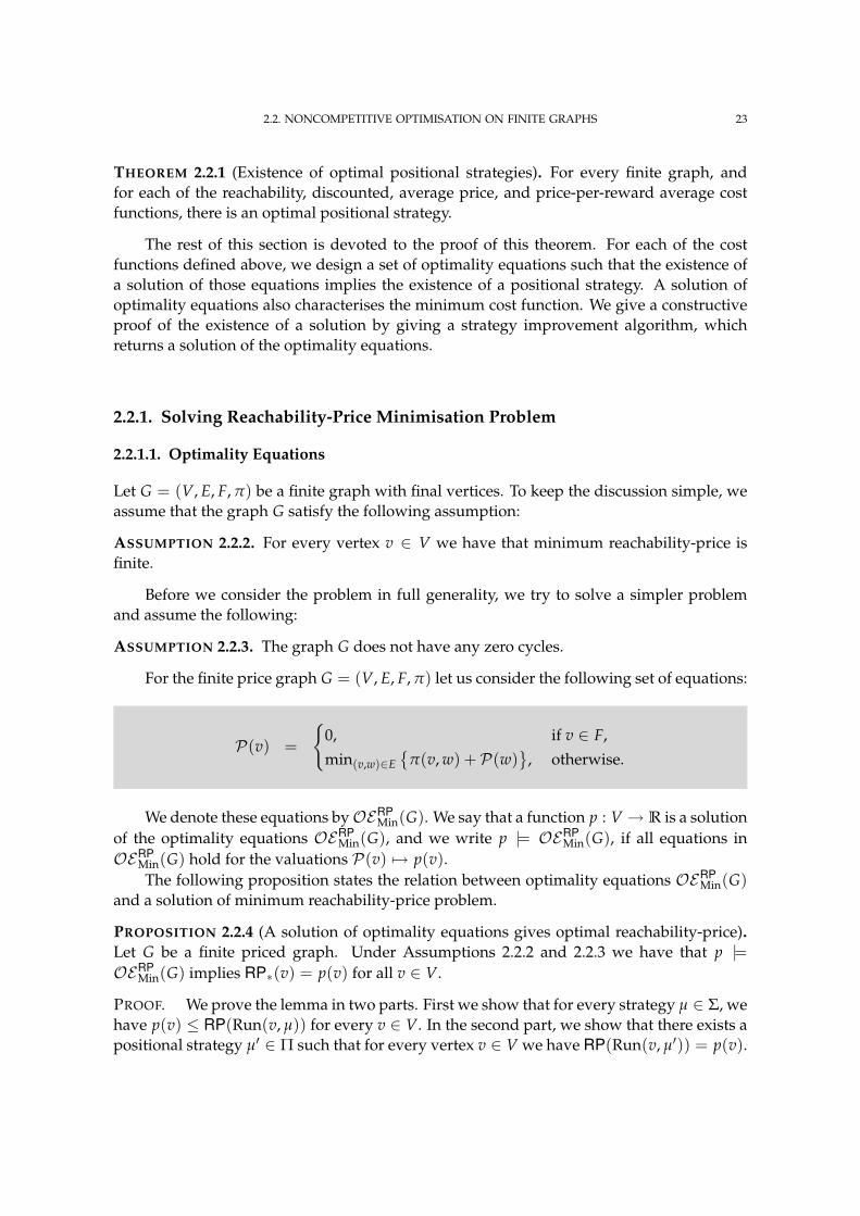
For the finite price graph G = (V, E, F, π) let us consider the following set of equations:
P(v) =
0, if v ∈ F,
min(v,w)∈E
π(v, w) + P(w)
, otherwise.
We denote these equations byOERPMin(G). We say that a function p : V → R is a solution
of the optimality equations OERPMin(G), and we write p |= OERP
Min(G), if all equations inOERP
Min(G) hold for the valuations P(v) 7→ p(v).The following proposition states the relation between optimality equations OERP
Min(G)and a solution of minimum reachability-price problem.
PROPOSITION 2.2.4 (A solution of optimality equations gives optimal reachability-price).Let G be a finite priced graph. Under Assumptions 2.2.2 and 2.2.3 we have that p |=OERP
Min(G) implies RP∗(v) = p(v) for all v ∈ V.
PROOF. We prove the lemma in two parts. First we show that for every strategy µ ∈ Σ, wehave p(v) ≤ RP(Run(v, µ)) for every v ∈ V. In the second part, we show that there exists apositional strategy µ′ ∈ Π such that for every vertex v ∈ V we have RP(Run(v, µ′)) = p(v).
2.2. NONCOMPETITIVE OPTIMISATION ON FINITE GRAPHS 24
– Let Run(v, µ) = 〈v = v0, v1, . . .〉 be the run from the vertex v according to thestrategy µ. Since p |= OERP
Min(G), for all i ≥ 0, we have the following.
p(vi) = 0 if vi ∈ F
p(vi) ≤ π(vi, vi+1) + p(vi+1), otherwise . (2.2.1)
Under Assumptions 2.2.2 and 2.2.3 we have that there is an index n ∈ N suchthat Stop(Run(v, µ)) = n. Summing (2.2.1) side-wise for 0 ≤ i < n, we get thefollowing.
p(v) ≤n
∑i=1
π(vi, vi−1) + p(vn).
Since vn ∈ F, we have p(vn) = 0 and we get the desired inequality.
p(v) ≤ RP(Run(v, µ)).
– For a set W the function Choose : 2W → W is defined such that for every setX ⊆ W we have Choose(X) ∈ X. In other words, Choose is a choice functionwhich for every non-empty set selects an element of this set. We fix an arbitrarychoice function for technical reasons, so that we have a way to canonically choosean arbitrary element from every non-empty set.
Let µ′ ∈ Π be the following positional strategy:
µ′(v) = Choose(argminw∈V
π(v, w) + p(w) : (v, w) ∈ E
).
Since p |= OERPMin(G), for such strategy µ′ it is straightforward to notice that for
all v ∈ V \ F we have:
p(v) = π(v, µ′(v)) + p(µ′(v)) . (2.2.2)
Let the run Run(v, µ′) be 〈v = v0, v1, v2, . . .〉. Again under Assumptions 2.2.2and 2.2.3 we have that there is an index n ∈ N such that Stop(Run(v, µ′)) = n.Summing (2.2.2) for all i, 0 ≤ i < n, we get the following.
p(v) =n
∑i=1
π(vi, vi−1) + p(vn).
Since vn ∈ F, we have p(vn) = 0 and we get the desired equality.
p(v) = RP(Run(v, µ′)).
We have thus shown that: for every strategy µ ∈ Σ, we have p(v) ≤ RP(Run(v, µ)) forevery v ∈ V; and there exists a positional strategy µ′ ∈ Π such that RP(Run(v, µ′)) = p(v)for every vertex v ∈ V. Hence it follows that p(v) = RP∗(v) for every vertex v ∈ V.
From the second part of the proof of the previous proposition, the following propositionfollows:
2.2. NONCOMPETITIVE OPTIMISATION ON FINITE GRAPHS 25
PROPOSITION 2.2.5 (A solution of optimality equations gives positional optimal strategy).Let G be a priced finite graph. Under Assumptions 2.2.2 and 2.2.3 we have that if there existsa solution of optimality equations OERP
Min(G) then there exists a positional optimal strategyfor minimum reachability-price problem.
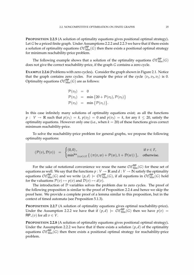
The following example shows that a solution of the optimality equations OERPMin(G)
does not give the correct reachability-price, if the graph G contains a zero cycle.
EXAMPLE 2.2.6 (Problems with zero cycles). Consider the graph shown in Figure 2.1. Noticethat the graph contains zero cycles. For example the price of the cycle 〈v1, v3, v1〉 is 0.Optimality equations OERP
Min(G) are as follows:
P(v2) = 0
P(v1) = min
20 + P(v2),P(v3)
P(v3) = minP(v1)
.
In this case infinitely many solutions of optimality equations exist; as all the functionsp : V → R such that p(v1) = k, p(v2) = 0 and p(v3) = k, for any k ≤ 20, satisfy theoptimality equations. However only one (i.e., when k = 20) of these functions gives correctminimum reachability-price.
To solve the reachability-price problem for general graphs, we propose the followingoptimality equations:
(P(v),D(v)) =
(0, 0) , if v ∈ F,
minlex(v,w)∈E
(π(v, w) + P(w), 1 +D(w))
, otherwise.
For the sake of notational convenience we reuse the name OERPMin(G) for these set of
equations as well. We say that the functions p : V → R and d : V →N satisfy the optimalityequations OERP
Min(G) and we write (p, d) |= OERPMin(G), if all equations in OERP
Min(G) holdfor the valuations P(v) 7→ p(v) and D(v) 7→ d(v).
The introduction of D variables solves the problem due to zero cycles. The proof ofthe following proposition is similar to the proof of Proposition 2.2.4 and hence we skip theproof here. We provide a complete proof of a lemma similar to this proposition, but in thecontext of timed automata (see Proposition 5.1.3).
PROPOSITION 2.2.7 (A solution of optimality equations gives optimal reachability-price).Under the Assumption 2.2.2 we have that if (p, d) |= OERP
Min(G) then we have p(v) =RP∗(v) for all v ∈ V.
PROPOSITION 2.2.8 (A solution of optimality equations gives positional optimal strategy).Under the Assumption 2.2.2 we have that if there exists a solution (p, d) of the optimalityequations OERP
Min(G) then there exists a positional optimal strategy for reachability-priceproblem.
2.2. NONCOMPETITIVE OPTIMISATION ON FINITE GRAPHS 26
In the rest of this subsection, we give a constructive proof of the following propositionby giving a strategy improvement algorithm which yields a solution of the optimalityequations OERP
Min(G).
PROPOSITION 2.2.9 (Existence of a solution). If the Assumption 2.2.2 holds then there existsa solution of the optimality equations OERP
Min(G).
2.2.1.2. Solving 0-player Optimality Equations
For a graph G = (V, E, F) and a positional strategy µ ∈ ΠMin, we define the graph Gµ =(V, E′, F) such that E′ = (v, µ(v)) : v ∈ V.
If the graph G = (V, E, F) is such that every vertex has a unique successor, i.e., for everyv ∈ V we have that the set E(v) = w : (v, w) ∈ E is a singleton, then we call such a grapha 0-player graph. Observe that for an arbitrary graph G and a positional strategy µ ∈ ΠMinthe graph Gµ is a 0-player graph. A 0-player priced graph is defined in straightforwardmanner.
For a 0-player priced graph G = (V, E, F, π), the optimality equations OERPMin(G) can
be rewritten in the following manner:
(P(v),D(v)) =
(0, 0) , if v ∈ F,
(π(v, E(v)) + P(E(v)), 1 +D(E(v))) , otherwise.
Remark. For brevity we have abused the notation to denote the unique vertex w such that(v, w) ∈ E by the singleton set E(v) containing w.
For a 0-player priced graph G, we write OERP(G) for these set of equations. The optimalityequations for 0-player reachability problem can be solved in time O(|V|).
2.2.1.3. Solving 1-player Optimality Equations
For given functions p : V → R and d : V → N, for every vertex v ∈ V, let us define the setM∗(v, p, d) as follows:
M∗(v, p, d) = argminlex
w∈V(π(v, w) + p(w), 1 + d(w)) : (v, w) ∈ E.
Consider the strategy improvement function ImproveMin : Π× [V → R]× [V →N] → Πdefined by:
ImproveMin(σ, p, d)(v) =
σ(v) if σ(v) ∈ M∗(v, p, d)Choose(M∗(v, p, d)) otherwise,
where p : V → R, d : V → N, and v ∈ V. From the definition of the function ImproveMin,the following proposition is immediate.
PROPOSITION 2.2.10 (Fixed point of ImproveMin are solutions of OERPMin(G)). Let µ ∈ ΠMin
and let (pµ, dµ) |= OERP(Gµ). If ImproveMin(µ, pµ, dµ) = µ then (pµ, dµ) |= OERPMin(G).
2.2. NONCOMPETITIVE OPTIMISATION ON FINITE GRAPHS 27
Input: A graph G = (V, E, F, π)Output: A solution of OERP
Min(G)begin1
(Initialisation). Choose an arbitrary positional strategy µ0 ∈ ΠMin;2
Set i = 0;3
repeat4
(Value Computation). Compute the solution (pi, di) of OERP(Gµi);5
(Strategy Improvement). Compute µi+1 = ImproveMin(µi, pi, di);6
Set i := i + 1;7
until µi+1 6= µi ;8
return (pi, di);9
end10
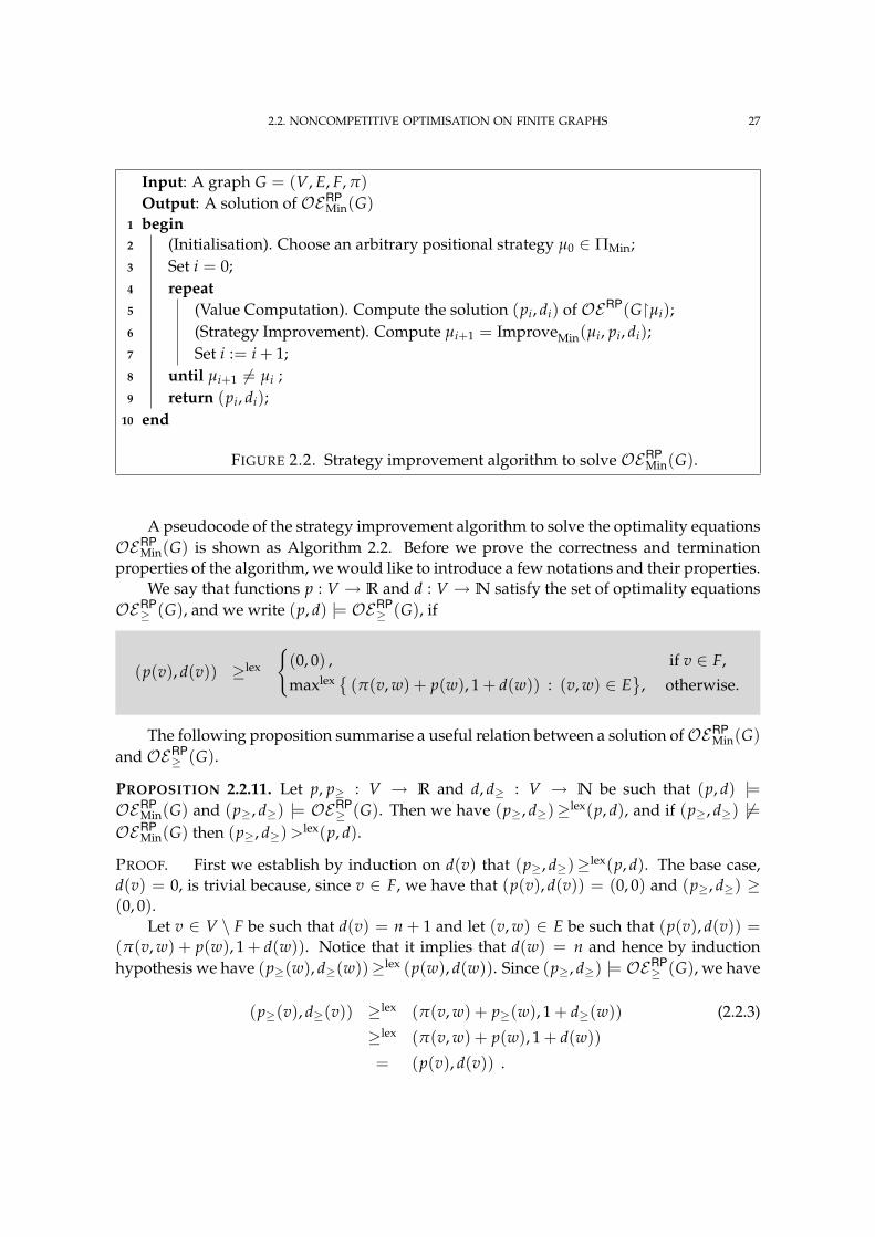
FIGURE 2.2. Strategy improvement algorithm to solve OERPMin(G).
A pseudocode of the strategy improvement algorithm to solve the optimality equationsOERP
Min(G) is shown as Algorithm 2.2. Before we prove the correctness and terminationproperties of the algorithm, we would like to introduce a few notations and their properties.
We say that functions p : V → R and d : V → N satisfy the set of optimality equationsOERP
≥ (G), and we write (p, d) |= OERP≥ (G), if
(p(v), d(v)) ≥lex
(0, 0) , if v ∈ F,
maxlex (π(v, w) + p(w), 1 + d(w)) : (v, w) ∈ E
, otherwise.
The following proposition summarise a useful relation between a solution ofOERPMin(G)
and OERP≥ (G).
PROPOSITION 2.2.11. Let p, p≥ : V → R and d, d≥ : V → N be such that (p, d) |=OERP
Min(G) and (p≥, d≥) |= OERP≥ (G). Then we have (p≥, d≥)≥lex(p, d), and if (p≥, d≥) 6|=
OERPMin(G) then (p≥, d≥) >lex(p, d).
PROOF. First we establish by induction on d(v) that (p≥, d≥)≥lex(p, d). The base case,d(v) = 0, is trivial because, since v ∈ F, we have that (p(v), d(v)) = (0, 0) and (p≥, d≥) ≥(0, 0).
Let v ∈ V \ F be such that d(v) = n + 1 and let (v, w) ∈ E be such that (p(v), d(v)) =(π(v, w) + p(w), 1 + d(w)). Notice that it implies that d(w) = n and hence by inductionhypothesis we have (p≥(w), d≥(w))≥lex (p(w), d(w)). Since (p≥, d≥) |= OERP
≥ (G), we have
(p≥(v), d≥(v)) ≥lex (π(v, w) + p≥(w), 1 + d≥(w)) (2.2.3)
≥lex (π(v, w) + p(w), 1 + d(w))= (p(v), d(v)) .
2.2. NONCOMPETITIVE OPTIMISATION ON FINITE GRAPHS 28
The second inequality follows from (p≥(w), d≥(w))≥lex (p(w), d(w)). This concludes theproof that (p≥, d≥)≥lex(p, d).
Now we prove that if (p≥, d≥) 6|= OERPMin(G) then there is a vertex v ∈ V such that
(p≥(v), d≥(v)) >lex(p(v), d(v)). Indeed, if (p≥, d≥) 6|= OERPMin(G) then either we have that
(p≥(v), d≥(v)) <lex(0, 0) for some vertex v ∈ F, or there is some vertex v ∈ V \ F such thatthe inequality (2.2.3) is strict and hence we get (p≥(v), d≥(v)) >lex(p(v), d(v)).
The following lemma states that every step of strategy improvement algorithm im-proves the strategy.
LEMMA 2.2.12 (Strict strategy improvement). Let µ, µ′ ∈ ΠMin, let (p, d) |= OERP(Gµ)and (p′, d′) |= OERP(Gµ′), and let µ′ = ImproveMin(µ, p, d). Then (p, d)≥lex(p′, d′) and ifµ 6= µ′ then (p, d) >lex(p′, d′).
PROOF. First we argue that (p, d) |= OERP≥ (Gµ′), which by Proposition 2.2.11 implies
that (p, d)≤lex(p′, d′). Indeed, for every v ∈ V \ F if µ(v) = w and µ′(v) = w′ then we have
(p(v), d(v)) = (π(v, w) + p(w), 1 + d(w)) , as (p, d) |= OERP(Gµ)
≥lex (π(v, w′) + p(w′), 1 + d(w′)
), by definition of ImproveMin.
Moreover, if µ 6= µ′ then there is a v ∈ V \ F for which the above inequality is strict.Then (p, d) 6|= OERP
Min(Gµ′), because every vertex in Gµ′ has a unique successor, and henceby Proposition 2.2.11 we conclude that (p, d) >lex(p′, d′).
LEMMA 2.2.13 (Correctness and termination of the strategy improvement algorithm). Thestrategy improvement algorithm for OERP
Min(G) terminates in finitely many steps andreturns a solution (p, d) of OERP
Min(G).
PROOF. Since the total number of positional strategies in a finite priced graph is finite(bounded from above by |V||V|), this lemma follows directly from Lemma 2.2.12 andProposition 2.2.10.
2.2.2. Solving Discounted-Price Minimisation Problem
For a priced graph G and a discount factor λ ∈ (0, 1), a solution of minimisation problemfor discounted-price function can be characterised by the following equations:
D(v) = min(v,w)∈E
(1− λ) · π(v, w) + λ · D(w)
, for all v ∈ V.
We denote these equations by OEDPMin(G, λ). We say that a function d : V → R is a solution
of the set of equations OEDPMin(G, λ), and we write d |= OEDP
Min(G, λ), if for all v ∈ V theequations in OEDP
Min(G, λ) holds for the valuation D(v) 7→ d(v).The following proposition shows that a solution of optimality equations OEDP
Min(G, λ)gives a solution of minimum discounted-price problem.
2.2. NONCOMPETITIVE OPTIMISATION ON FINITE GRAPHS 29
PROPOSITION 2.2.14 (A solution of optimality equations gives optimal discounted price).For a priced graph G and a discount factor λ ∈ (0, 1), if d |= OEDP
Min(G, λ) then for all v ∈ Vwe have that d(v) = DP(λ)∗(v).
PROOF. Let d |= OEDPMin(G, λ). There are two parts of the proof of this lemma. First we
show that for every strategy µ ∈ ΣMin we have that d(v) ≤ DP(λ)(Run(v, µ)) for everyv ∈ V. In the second part we show that there exists a positional strategy µ′ ∈ ΠMin suchthat for every vertex v ∈ V we have that d(v) = DP(λ)(Run(v, µ′)).
– Let µ be an arbitrary strategy and let Run(v, µ) be the sequence 〈v0 = v, v1, v2, . . .〉.Since d |= OEDP
Min(G, λ), for all i ≥ 0 we have that
d(vi) ≤ (1− λ) · π(vi, vi+1) + λ · d(vi+1).
For all 0 ≤ i < n multiplying both sides of this equation by λi and summing side-wise we get the following inequality:
d(v0) ≤ (1− λ)n−1
∑i=0
λi · π(vi, vi+1) + λn · d(vn).
Taking limit of both sides we get the desired inequality:
d(v) = d(v0) ≤ DP(λ)(Run(v, µ)).
– Let µ′ ∈ ΠMin be the following positional strategy: for all v ∈ V we have that
µ′(v) = Choose(argminw∈V
(1− λ) · π(v, w) + λ · d(w) : (v, w) ∈ E
).
Since d : V → R is a solution of optimality equations OEDPMin(G, λ), from previous
equation it follows that for all v ∈ V we have
d(v) = (1− λ) · π(v, µ′(v)) + λ · d(µ′(v)).
By doing a similar analysis to that in the previous part of this proof, it can be shownthat:
d(v) = DP(λ)(Run(v, µ′)).
From the second part of the proof of the previous proposition, the following propositionis immediate.
PROPOSITION 2.2.15 (A solution of optimality equations gives positional optimal strategy).If there exists a solution of optimality equations OEDP
Min(G, λ) then there exists a positionaloptimal strategy for minimum discounted-price problem.
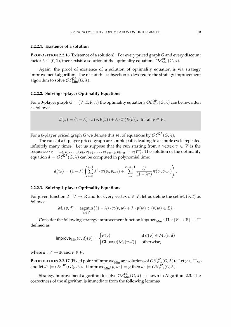
2.2. NONCOMPETITIVE OPTIMISATION ON FINITE GRAPHS 30
2.2.2.1. Existence of a solution
PROPOSITION 2.2.16 (Existence of a solution). For every priced graph G and every discountfactor λ ∈ (0, 1), there exists a solution of the optimality equations OEDP
Min(G, λ).
Again, the proof of existence of a solution of optimality equation is via strategyimprovement algorithm. The rest of this subsection is devoted to the strategy improvementalgorithm to solve OEDP
Min(G, λ).
2.2.2.2. Solving 0-player Optimality Equations
For a 0-player graph G = (V, E, F, π) the optimality equationsOEDPMin(G, λ) can be rewritten
as follows:
D(v) = (1− λ) · π(v, E(v)) + λ · D(E(v)), for all v ∈ V.
For a 0-player priced graph G we denote this set of equations by OEDP(G, λ).The runs of a 0-player priced graph are simple paths leading to a simple cycle repeated
infinitely many times. Let us suppose that the run starting from a vertex v ∈ V is thesequence 〈v = v0, v1, . . . , (vk, vk+1, . . . , vk+n−1, vk+n = vk)ω〉. The solution of the optimalityequation d |= OEDP(G, λ) can be computed in polynomial time:
d(v0) = (1− λ)
(k−1
∑i=0
λi · π(vi, vi+1) +k+n−1
∑i=k
λi
(1− λn)π(vi, vi+1)
).
2.2.2.3. Solving 1-player Optimality Equations
For given function d : V → R and for every vertex v ∈ V, let us define the set M∗(v, d) asfollows:
M∗(v, d) = argminw∈V
(1− λ) · π(v, w) + λ · p(w) : (v, w) ∈ E.
Consider the following strategy improvement function ImproveMin : Π× [V → R]→ Πdefined as
ImproveMin(σ, d)(v) =
σ(v) if σ(v) ∈ M∗(v, d)Choose(M∗(v, d)) otherwise,
where d : V → R and v ∈ V.
PROPOSITION 2.2.17 (Fixed point of ImproveMin are solutions ofOEDPMin(G, λ)). Let µ ∈ ΠMin
and let dµ |= OEDP(Gµ, λ). If ImproveMin(µ, dµ) = µ then dµ |= OEDPMin(G, λ).
Strategy improvement algorithm to solve OEDPMin(G, λ) is shown in Algorithm 2.3. The
correctness of the algorithm is immediate from the following lemmas.
2.2. NONCOMPETITIVE OPTIMISATION ON FINITE GRAPHS 31
Input: A graph G = (V, E, F, π) and λ ∈ (0, 1)Output: A solution of OEDP
Min(G, λ)begin1
(Initialisation). Choose an arbitrary positional strategy µ0 ∈ ΠMin;2
Set i = 0;3
repeat4
(Value Computation). Compute the solution di of OEDP(Gµi, λ);5
(Strategy Improvement). Compute µi+1 = ImproveMin(µi, di);6
Set i := i + 1;7
until µi+1 6= µi ;8
return di;9
end10
FIGURE 2.3. Strategy improvement algorithm to solve OEDPMin(G, λ).
LEMMA 2.2.18 (Strict strategy improvement for Min). Let strategies µ, µ′ ∈ ΠMin, let d |=OEDP(Gµ, λ) and d′ |= OEDP(Gµ′, λ), and let µ′ = ImproveMin(µ, d). Then d ≥ d′ and ifµ 6= µ′ then d > d′.
LEMMA 2.2.19 (Correctness and termination of the strategy improvement algorithm). Thestrategy improvement algorithm for OEDP
Min(G, λ) terminates in finitely many steps andreturns a solution of OEDP
Min(G, λ).
2.2.3. Solving Average-price and Price-per-reward Average Minimisation Prob-lems
It is easy to see that average-price minimisation problems are special cases of price-per-reward average minimisation problems, where the reward function $ : E → R is such that$(e) = 1, for every edge e ∈ E. Hence we shall not discuss the average-price minimisationproblem separately.
Given a graph G = (V, E, F, π, $) the following equations capture the optimal price-per-reward average cost:
G(v) = min(v,w)∈E
G(w)
, for all v ∈ V, and
B(v) = min(v,w)∈E
π(v, w)− $(v, w) · G(v) + B(w) : G(v) = G(w)
for all v ∈ V.
Sometimes we write these equations in the following compact form. It is routine to verifythat the two sets of equations are equivalent.
(G(v),B(v)) = minlex
(v,w)∈E
(G(w), π(v, w)− $(v, w) · G(v) + B(w))
for all v ∈ V.
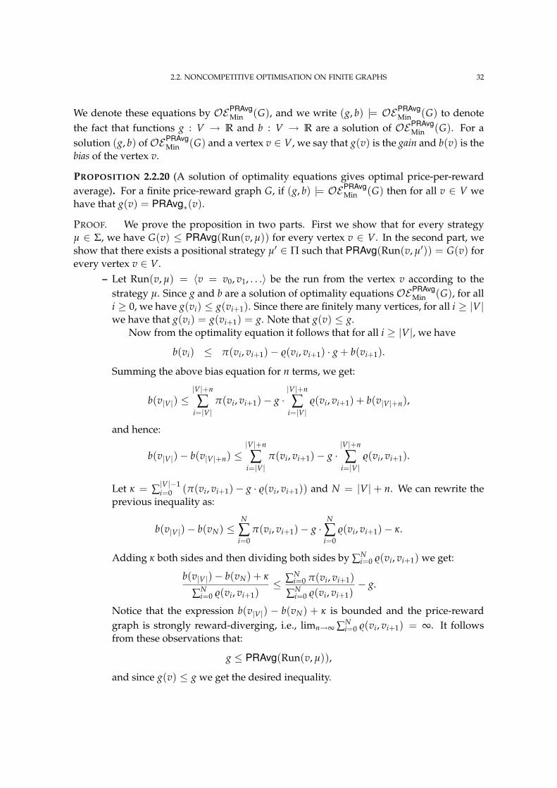
2.2. NONCOMPETITIVE OPTIMISATION ON FINITE GRAPHS 32
We denote these equations by OEPRAvgMin (G), and we write (g, b) |= OEPRAvg
Min (G) to denotethe fact that functions g : V → R and b : V → R are a solution of OEPRAvg
Min (G). For asolution (g, b) ofOEPRAvg
Min (G) and a vertex v ∈ V, we say that g(v) is the gain and b(v) is thebias of the vertex v.
PROPOSITION 2.2.20 (A solution of optimality equations gives optimal price-per-rewardaverage). For a finite price-reward graph G, if (g, b) |= OEPRAvg
Min (G) then for all v ∈ V wehave that g(v) = PRAvg∗(v).
PROOF. We prove the proposition in two parts. First we show that for every strategyµ ∈ Σ, we have G(v) ≤ PRAvg(Run(v, µ)) for every vertex v ∈ V. In the second part, weshow that there exists a positional strategy µ′ ∈ Π such that PRAvg(Run(v, µ′)) = G(v) forevery vertex v ∈ V.
– Let Run(v, µ) = 〈v = v0, v1, . . .〉 be the run from the vertex v according to thestrategy µ. Since g and b are a solution of optimality equations OEPRAvg
Min (G), for alli ≥ 0, we have g(vi) ≤ g(vi+1). Since there are finitely many vertices, for all i ≥ |V|we have that g(vi) = g(vi+1) = g. Note that g(v) ≤ g.
Now from the optimality equation it follows that for all i ≥ |V|, we have
b(vi) ≤ π(vi, vi+1)− $(vi, vi+1) · g + b(vi+1).
Summing the above bias equation for n terms, we get:
b(v|V|) ≤|V|+n
∑i=|V|
π(vi, vi+1)− g ·|V|+n
∑i=|V|
$(vi, vi+1) + b(v|V|+n),
and hence:
b(v|V|)− b(v|V|+n) ≤|V|+n
∑i=|V|
π(vi, vi+1)− g ·|V|+n
∑i=|V|
$(vi, vi+1).
Let κ = ∑|V|−1i=0 (π(vi, vi+1)− g · $(vi, vi+1)) and N = |V| + n. We can rewrite the
previous inequality as:
b(v|V|)− b(vN) ≤N
∑i=0
π(vi, vi+1)− g ·N
∑i=0
$(vi, vi+1)− κ.
Adding κ both sides and then dividing both sides by ∑Ni=0 $(vi, vi+1) we get:
b(v|V|)− b(vN) + κ
∑Ni=0 $(vi, vi+1)
≤ ∑Ni=0 π(vi, vi+1)
∑Ni=0 $(vi, vi+1)
− g.
Notice that the expression b(v|V|) − b(vN) + κ is bounded and the price-rewardgraph is strongly reward-diverging, i.e., limn→∞ ∑N
i=0 $(vi, vi+1) = ∞. It followsfrom these observations that:
g ≤ PRAvg(Run(v, µ)),
and since g(v) ≤ g we get the desired inequality.
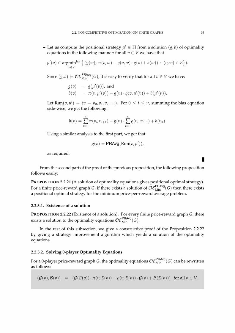
2.2. NONCOMPETITIVE OPTIMISATION ON FINITE GRAPHS 33
– Let us compute the positional strategy µ′ ∈ Π from a solution (g, b) of optimalityequations in the following manner: for all v ∈ V we have that
µ′(v) ∈ argminlex
w∈V
(g(w), π(v, w)− $(v, w) · g(v) + b(w)) : (v, w) ∈ E
).
Since (g, b) |= OEPRAvgMin (G), it is easy to verify that for all v ∈ V we have:
g(v) = g(µ′(v)), and
b(v) = π(v, µ′(v))− g(v) · $(v, µ′(v)) + b(µ′(v)).
Let Run(v, µ′) = 〈v = v0, v1, v2, . . .〉. For 0 ≤ i ≤ n, summing the bias equationside-wise, we get the following:
b(v) =n
∑i=0
π(vi, vi+1)− g(v) ·n
∑i=0
$(vi, vi+1) + b(vn).
Using a similar analysis to the first part, we get that
g(v) = PRAvg(Run(v, µ′)),
as required.
From the second part of the proof of the previous proposition, the following propositionfollows easily:
PROPOSITION 2.2.21 (A solution of optimality equations gives positional optimal strategy).For a finite price-reward graph G, if there exists a solution of OEPRAvg
Min (G) then there existsa positional optimal strategy for the minimum price-per-reward average problem.
2.2.3.1. Existence of a solution
PROPOSITION 2.2.22 (Existence of a solution). For every finite price-reward graph G, thereexists a solution to the optimality equations OEPRAvg
Min (G).
In the rest of this subsection, we give a constructive proof of the Proposition 2.2.22by giving a strategy improvement algorithm which yields a solution of the optimalityequations.
2.2.3.2. Solving 0-player Optimality Equations
For a 0-player price-reward graph G, the optimality equationsOEPRAvgMin (G) can be rewritten
as follows:
(G(v),B(v)) = (G(E(v)), π(v, E(v))− $(v, E(v)) · G(v) + B(E(v))) for all v ∈ V.
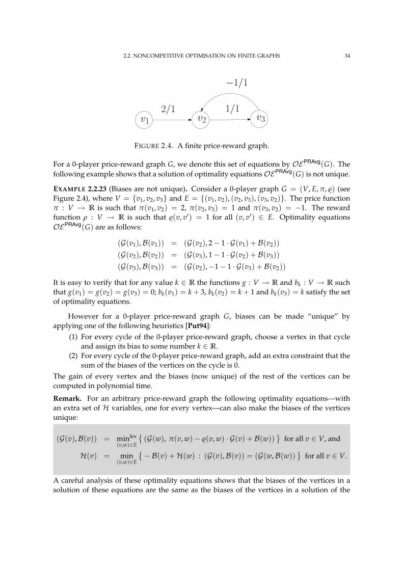
2.2. NONCOMPETITIVE OPTIMISATION ON FINITE GRAPHS 34
v1 v2 v32/1 1/1
−1/1
FIGURE 2.4. A finite price-reward graph.
For a 0-player price-reward graph G, we denote this set of equations by OEPRAvg(G). Thefollowing example shows that a solution of optimality equationsOEPRAvg(G) is not unique.
EXAMPLE 2.2.23 (Biases are not unique). Consider a 0-player graph G = (V, E, π, $) (seeFigure 2.4), where V = v1, v2, v3 and E = (v1, v2), (v2, v3), (v3, v2). The price functionπ : V → R is such that π(v1, v2) = 2, π(v2, v3) = 1 and π(v3, v2) = −1. The rewardfunction ρ : V → R is such that $(v, v′) = 1 for all (v, v′) ∈ E. Optimality equationsOEPRAvg(G) are as follows:
(G(v1),B(v1)) = (G(v2), 2− 1 · G(v1) + B(v2))
(G(v2),B(v2)) = (G(v3), 1− 1 · G(v2) + B(v3))
(G(v3),B(v3)) = (G(v2),−1− 1 · G(v3) + B(v2))
It is easy to verify that for any value k ∈ R the functions g : V → R and bk : V → R suchthat g(v1) = g(v2) = g(v3) = 0; bk(v1) = k + 3, bk(v2) = k + 1 and bk(v3) = k satisfy the setof optimality equations.
However for a 0-player price-reward graph G, biases can be made “unique” byapplying one of the following heuristics [Put94]:
(1) For every cycle of the 0-player price-reward graph, choose a vertex in that cycleand assign its bias to some number k ∈ R.
(2) For every cycle of the 0-player price-reward graph, add an extra constraint that thesum of the biases of the vertices on the cycle is 0.
The gain of every vertex and the biases (now unique) of the rest of the vertices can becomputed in polynomial time.
Remark. For an arbitrary price-reward graph the following optimality equations—withan extra set of H variables, one for every vertex—can also make the biases of the verticesunique:
(G(v),B(v)) = minlex
(v,w)∈E
(G(w), π(v, w)− $(v, w) · G(v) + B(w))
for all v ∈ V, and
H(v) = min(v,w)∈E
−B(v) +H(w) : (G(v),B(v)) = (G(w,B(w))
for all v ∈ V.
A careful analysis of these optimality equations shows that the biases of the vertices in asolution of these equations are the same as the biases of the vertices in a solution of the
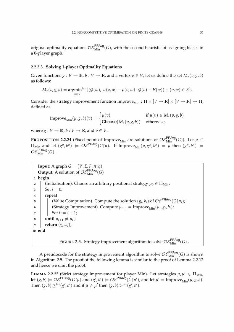
2.2. NONCOMPETITIVE OPTIMISATION ON FINITE GRAPHS 35
original optimality equations OEPRAvgMin (G), with the second heuristic of assigning biases in
a 0-player graph.
2.2.3.3. Solving 1-player Optimality Equations
Given functions g : V → R, b : V → R, and a vertex v ∈ V, let us define the set M∗(v, g, b)as follows:
M∗(v, g, b) = argminlex
w∈V(G(w), π(v, w)− $(v, w) · G(v) + B(w)) : (v, w) ∈ E.
Consider the strategy improvement function ImproveMin : Π× [V → R]× [V → R] → Π,defined as
ImproveMin(µ, g, b)(v) =
µ(v) if µ(v) ∈ M∗(v, g, b)Choose(M∗(v, g, b)) otherwise,
where g : V → R, b : V → R, and v ∈ V.
PROPOSITION 2.2.24 (Fixed point of ImproveMin are solutions of OEPRAvgMin (G)). Let µ ∈
ΠMin and let (gµ, bµ) |= OEPRAvg(Gµ). If ImproveMin(µ, gµ, bµ) = µ then (gµ, bµ) |=OEPRAvg
Min (G).
Input: A graph G = (V, E, F, π, $)Output: A solution of OEPRAvg
Min (G)begin1
(Initialisation). Choose an arbitrary positional strategy µ0 ∈ ΠMin;2
Set i = 0;3
repeat4
(Value Computation). Compute the solution (gi, bi) of OEPRAvg(Gµi);5
(Strategy Improvement). Compute µi+1 = ImproveMin(µi, gi, bi);6
Set i := i + 1;7
until µi+1 6= µi ;8
return (gi, bi);9
end10
FIGURE 2.5. Strategy improvement algorithm to solve OEPRAvgMin (G) .
A pseudocode for the strategy improvement algorithm to solve OEPRAvgMin (G) is shown
in Algorithm 2.5. The proof of the following lemma is similar to the proof of Lemma 2.2.12and hence we omit the proof.
LEMMA 2.2.25 (Strict strategy improvement for player Min). Let strategies µ, µ′ ∈ ΠMin,let (g, b) |= OEPRAvg(Gµ) and (g′, b′) |= OEPRAvg(Gµ′), and let µ′ = ImproveMin(µ, g, b).Then (g, b)≥lex(g′, b′) and if µ 6= µ′ then (g, b) >lex(g′, b′).
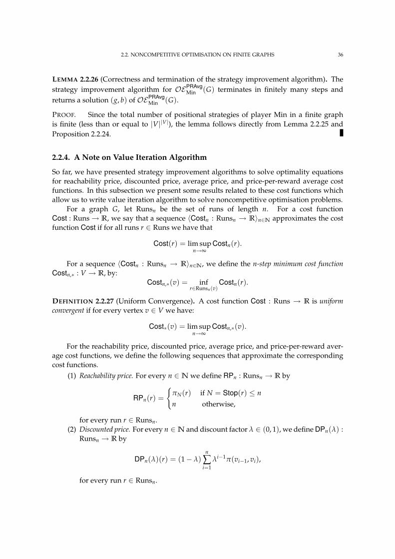
2.2. NONCOMPETITIVE OPTIMISATION ON FINITE GRAPHS 36
LEMMA 2.2.26 (Correctness and termination of the strategy improvement algorithm). Thestrategy improvement algorithm for OEPRAvg
Min (G) terminates in finitely many steps andreturns a solution (g, b) of OEPRAvg
Min (G).
PROOF. Since the total number of positional strategies of player Min in a finite graphis finite (less than or equal to |V||V|), the lemma follows directly from Lemma 2.2.25 andProposition 2.2.24.
2.2.4. A Note on Value Iteration Algorithm
So far, we have presented strategy improvement algorithms to solve optimality equationsfor reachability price, discounted price, average price, and price-per-reward average costfunctions. In this subsection we present some results related to these cost functions whichallow us to write value iteration algorithm to solve noncompetitive optimisation problems.
For a graph G, let Runsn be the set of runs of length n. For a cost functionCost : Runs→ R, we say that a sequence 〈Costn : Runsn → R〉n∈N approximates the costfunction Cost if for all runs r ∈ Runs we have that
Cost(r) = lim supn→∞
Costn(r).
For a sequence 〈Costn : Runsn → R〉n∈N, we define the n-step minimum cost functionCostn,∗ : V → R, by:
Costn,∗(v) = infr∈Runsn(v)
Costn(r).
DEFINITION 2.2.27 (Uniform Convergence). A cost function Cost : Runs → R is uniformconvergent if for every vertex v ∈ V we have:
Cost∗(v) = lim supn→∞
Costn,∗(v).
For the reachability price, discounted price, average price, and price-per-reward aver-age cost functions, we define the following sequences that approximate the correspondingcost functions.
(1) Reachability price. For every n ∈N we define RPn : Runsn → R by
RPn(r) =
πN(r) if N = Stop(r) ≤ nn otherwise,
for every run r ∈ Runsn.(2) Discounted price. For every n ∈N and discount factor λ ∈ (0, 1), we define DPn(λ) :
Runsn → R by
DPn(λ)(r) = (1− λ)n
∑i=1
λi−1π(vi−1, vi),
for every run r ∈ Runsn.
2.3. GAMES ON FINITE GRAPHS 37
(3) Average price. For every n ∈N we define APn : Runsn → R by
APn(r) =πn(r)
n,
for every run r ∈ Runsn.(4) Price-per-reward average. Finally, for every n ∈ N we define PRAvgn : Runsn → R
by
PRAvgn(r) =πn(r)$n(r)
,
for every run r ∈ Runsn.
Notice that if the cost functions RP, DP, AP, and PRAvg are uniform convergent, thenthe value iteration method for these problems is immediate: at every iteration n, generatesuccessively the corresponding n-step minimum cost Costn(v) for every vertex v ∈ V.
THEOREM 2.2.28 (Uniform convergence). For a finite graph, the following cost functionsare uniform convergent: reachability price (Proposition 2.1.2 in [Ber01]), discounted price(Proposition 1.2 in [Ber01]), average price (Section 7.4 in [Ber95]), and price-per-rewardaverage (Section 7.4 in [Ber95]).
2.3. Games on Finite GraphsDEFINITION 2.3.1 (Game Graph). A finite game graph is a tuple Γ = (V, E, VMin, VMax),where:
– (V, E) is a finite graph,– VMin ⊆ V is the set of vertices controlled by player Min, and– VMax ⊆ V is the set of vertices controlled by player Max.
We require that the sets VMax and VMin form a partition of the set of vertices V.
Let us fix a finite game automaton Γ = (G, VMin, VMax) for the rest of this section.In the context of games we sometimes refer to a run as a play of the game. A play starts
at a vertex v0 ∈ V. If v0 ∈ Vp, for p ∈ Max, Min , then player p chooses a successor of thecurrent vertex v0, i.e., a vertex v1, such that (v0, v1) ∈ E, and v1 becomes the new currentvertex. When this happens then we say that player p has made a move from the currentvertex. Players keep making moves in this fashion indefinitely thus forming an infinite run〈v0, v1, v2, . . .〉 in the game graph.
DEFINITION 2.3.2 (Cost Game on a Finite Game Graph). A cost game on a finite game graphis a tuple (Γ, CostMin, CostMax), where:
– Γ = (V, E, VMin, VMax) is a game graph,– CostMin : Runs→ R is a payoff function for player Min, that gives the amount Min
loses in a play, and– CostMax : Runs → R is the payoff function for player Max, that gives the amount
Max wins in a play.
2.3. GAMES ON FINITE GRAPHS 38
A cost game is called zero-sum if we have that CostMin(r) = CostMax(r) for every play rof the game.
A strategy for the player Min is a (partial) function µ : Runsfin → V such that for everyrun r = 〈v0, v1, . . . , vn〉 if vn ∈ VMin then µ(r) is defined and it is such that (vn, µ(r)) ∈ E.Similarly we define a strategy for the player Max. We write ΣMin for the set of strategies ofplayer Min and ΣMax for the set of strategies of player Max. For strategies µ ∈ ΣMin andχ ∈ ΣMax, and for an initial vertex v ∈ V, we write Run(v, µ, χ) for the unique path formedif the game starts in the vertex v and then players use strategies µ and χ, respectively.
The upper value Val(v) of a vertex v ∈ V is defined by:
Val(v) = infµ∈ΣMin
supχ∈ΣMax
CostMin(Run(v, µ, χ)),
and the lower value Val(v) of a vertex v ∈ V is defined by:
Val(v) = supχ∈ΣMax
infµ∈ΣMin
CostMax(Run(v, µ, χ)).
We say that the game is determined if for all v ∈ V we have Val(v) = Val(v). In this case wesay that the value Val(v) exists and it is Val(v) = Val(v) = Val(v). We say that the strategiesµ∗ ∈ ΣMin and χ∗ ∈ ΣMax are optimal for the respective players if for all v ∈ V we have that
infµ∈ΣMin
CostMax(Run(v, µ, χ∗)) = Val(v) = supχ∈ΣMax
CostMin(Run(v, µ∗, χ)).
Let ΠMin and ΠMax be the set of positional strategies of player Min and player Max,respectively. We say that a game is positionally determined if players have positional optimalstrategies.
If a cost game is determined, then the competitive optimisation problem for a cost game(Γ, CostMin, CostMax) is: “given a graph graph Γ, a vertex v ∈ V and a number D ∈ Q,determine whether Val(v) ≤ D.”
We consider the following cost games in this chapter:(1) Reachability-price game. A reachability-price game (Γ, RPMin, RPMax) has the follow-
ing payoff functions:
RPMin(r) = RPMax(r) =
πN(r) if N = Stop(r) < ∞∞ otherwise.
(2) Discounted-price game. For a given discount factor λ ∈ (0, 1), a discounted-pricegame (Γ, DPMin(λ), DPMax(λ)) has the following payoff functions:
DPMin(λ)(r) = DPMax(λ)(r) = (1− λ)∞
∑i=1
λi−1π(vi−1, vi).
(3) Average-price game. An average-price game (Γ, APMin, APMax) has the followingpayoff functions:
APMin(r) = lim supn→∞
πn(r)n
and APMax(r) = lim infn→∞
πn(r)n
.
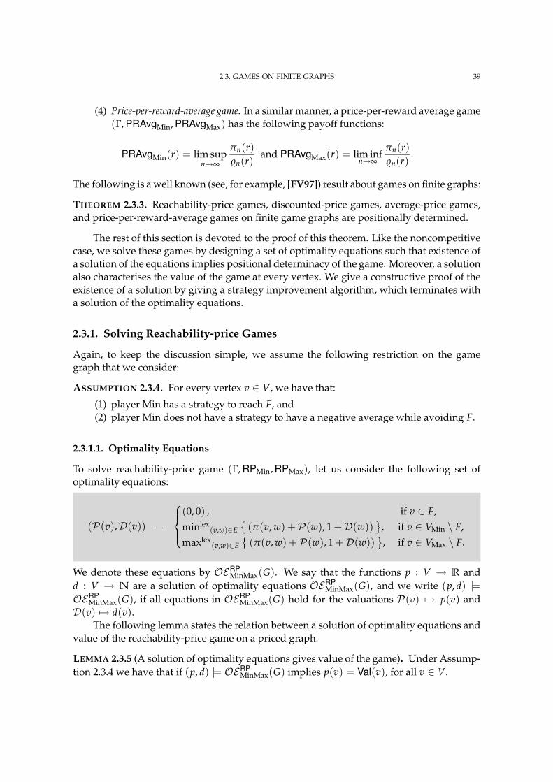
2.3. GAMES ON FINITE GRAPHS 39
(4) Price-per-reward-average game. In a similar manner, a price-per-reward average game(Γ, PRAvgMin, PRAvgMax) has the following payoff functions:
PRAvgMin(r) = lim supn→∞
πn(r)$n(r)
and PRAvgMax(r) = lim infn→∞
πn(r)$n(r)
.
The following is a well known (see, for example, [FV97]) result about games on finite graphs:
THEOREM 2.3.3. Reachability-price games, discounted-price games, average-price games,and price-per-reward-average games on finite game graphs are positionally determined.
The rest of this section is devoted to the proof of this theorem. Like the noncompetitivecase, we solve these games by designing a set of optimality equations such that existence ofa solution of the equations implies positional determinacy of the game. Moreover, a solutionalso characterises the value of the game at every vertex. We give a constructive proof of theexistence of a solution by giving a strategy improvement algorithm, which terminates witha solution of the optimality equations.
2.3.1. Solving Reachability-price Games
Again, to keep the discussion simple, we assume the following restriction on the gamegraph that we consider:
ASSUMPTION 2.3.4. For every vertex v ∈ V, we have that:
(1) player Min has a strategy to reach F, and(2) player Min does not have a strategy to have a negative average while avoiding F.
2.3.1.1. Optimality Equations
To solve reachability-price game (Γ, RPMin, RPMax), let us consider the following set ofoptimality equations:
(P(v),D(v)) =
(0, 0) , if v ∈ F,
minlex(v,w)∈E
(π(v, w) + P(w), 1 +D(w))
, if v ∈ VMin \ F,
maxlex(v,w)∈E
(π(v, w) + P(w), 1 +D(w))
, if v ∈ VMax \ F.
We denote these equations by OERPMinMax(G). We say that the functions p : V → R and
d : V → N are a solution of optimality equations OERPMinMax(G), and we write (p, d) |=
OERPMinMax(G), if all equations in OERP
MinMax(G) hold for the valuations P(v) 7→ p(v) andD(v) 7→ d(v).
The following lemma states the relation between a solution of optimality equations andvalue of the reachability-price game on a priced graph.
LEMMA 2.3.5 (A solution of optimality equations gives value of the game). Under Assump-tion 2.3.4 we have that if (p, d) |= OERP
MinMax(G) implies p(v) = Val(v), for all v ∈ V.
2.3. GAMES ON FINITE GRAPHS 40
PROOF. Let (p, d) |= OERPMinMax(G). Using this solution of the optimality equation, let us
define the positional strategy µ∗ of player Min as follows: for every vertex v ∈ VMin, wehave:
µ∗(v) ∈ argminlex
w∈V
(π(v, w) + p(w), 1 + d(w)) : (v, w) ∈ E
.
Similarly we define the positional strategy χ∗ as follows: for every vertex v ∈ VMax, we have:
χ∗(v) ∈ argmaxlex
w∈V
(π(v, w) + p(w), 1 + d(w)) : (v, w) ∈ E
.
Note that the strategies µ∗ and χ∗ are defined in such a way that for all v ∈ VMin, we havep(v) = π(v, µ∗(v)) + p(µ∗(v)), and for all v ∈ VMax, we have that p(v) = π(v, χ∗(v)) +p(χ∗(v)). It is easy to verify that p(v) = RP(Run(v, µ∗, χ∗). Now to prove the lemma, whatremains to be shown is that µ∗ ∈ ΣMin and χ∗ ∈ ΣMax are optimal strategies.
The rest of the proof is in two parts. In first part we show that p(v) ≥ Val(v) and in thesecond part we show that p(v) ≤ Val(v).
– Let µ ∈ ΣMin be a strategy (not necessarily positional) of player Min and let usconsider the initial vertex v ∈ V. Let the run Run(v, µ, χ∗) be 〈v0 = v, v1, v2, . . .〉.For all i ≥ 0, if vi ∈ VMin then we have the following inequality:
(p(vi), d(vi))≤lex (π(vi, vi+1) + p(vi+1), 1 + d(vi+1) ,
as (p, d) is a solution of optimality equations OERPMinMax(G). Moreover for all i ≥ 0,
if vi ∈ VMax then from the definition of χ∗ we get the equality:
(p(vi), d(vi)) = (π(vi, vi+1) + p(vi+1), 1 + d(vi+1) .
Hence it implies that for all i ≥ 0 we have
p(vi) ≤ π(vi, vi+1) + p(vi+1). (2.3.1)
If Stop(Run(v, µ, χ∗)) = ∞ then by definition we have that RP(Run(v, µ, χ∗)) = ∞,and then is inequality p(vi) ≤ RP(Run(v, µ, χ∗)) is trivial. Let us assume thatStop(Run(v, µ, χ∗)) = n < ∞. Summing the inequalities (2.3.1) for 0 ≤ i < n,side-wise we get:
p(v0) ≤Stop(Run(v,µ,χ∗))−1
∑i=0
π(vi, vi+1) + p(vn).
Since vn ∈ F, we have that p(vn) = 0; also note that v0 = v. It follows that for everystrategy µ ∈ ΣMin we have that p(v) ≤ RP(Run(v, µ, χ∗). Since µ∗ ∈ ΣMin we havethat
p(v) ≤ RP(Run(v, µ∗, χ∗)) = Val(v).
– Let χ ∈ ΣMax be an arbitrary strategy of player Max and let us consider the initialvertex v ∈ V. Let the run Run(v, µ∗, χ) be 〈v0 = v, v1, v2, . . .〉. For all i ≥ 0, ifvi ∈ VMax then we have the following inequality:
(p(vi), d(vi))≥lex (π(vi, vi+1) + p(vi+1), 1 + d(vi+1) ,
2.3. GAMES ON FINITE GRAPHS 41
as (p, d) is a solution of optimality equations OERPMinMax(G). Moreover for all i ≥ 0,
if vi ∈ VMin then from the definition of µ∗ we get the equality:
(p(vi), d(vi)) = (π(vi, vi+1) + p(vi+1), 1 + d(vi+1) .
Hence it implies that for all i ≥ 0 we have
p(vi) ≥ π(vi, vi+1) + p(vi+1).
If Stop(Run(v, µ∗, χ)) = ∞ then it is easy to verify that either the player Min doesnot have a strategy to reach F, or the strategy µ∗ have negative average whileavoiding F. Since both cases are not possible due to Assumption 2.3.4, we knowthat Stop(Run(v, µ∗, χ)) = n < ∞ Now using a similar analysis to the first part, itis straightforward to verify that
p(v) ≥ Val(v).
From the second part of the proof of the previous lemma, the following proposition isimmediate.
PROPOSITION 2.3.6 (A solution of optimality equations gives positional optimal strategiesfor both players). For a priced graph G, if there exists a solution of OERP
MinMax(G) then bothplayers have positional optimal strategies.
We prove the following lemma using a strategy improvement algorithm, which upontermination gives a solution of the optimality equations.
LEMMA 2.3.7 (Existence of a solution). For every priced graph G, there exists a solution ofthe optimality equations OERP
MinMax(G).
2.3.1.2. Solving 2-player Optimality Equations
For given functions p : V → R and d : V → N, let us define the set M∗(v, p, d) for everyvertex v ∈ V as follows:
M∗(v, p, d) = argmaxlex
w∈V(π(v, w) + p(w), 1 + d(w)) : (v, w) ∈ E.
Consider the strategy improvement function ImproveMax : ΠMax × [V → R]× [V →N] →ΠMax defined by:
ImproveMax(χ, p, d)(v) =
χ(v) if χ(v) ∈ M∗(v, p, d)Choose(M∗(v, p, d)) otherwise,
where p : V → R, d : V →N, and v ∈ V.
PROPOSITION 2.3.8 (Fixed points of ImproveMax are solutions of OERPMinMax). Let χ ∈
ΠMax and let (pχ, dχ) |= OERPMin(Gχ). If ImproveMax(χ, pχ, dχ) = χ then (pχ, dχ) |=
OERPMinMax(G).
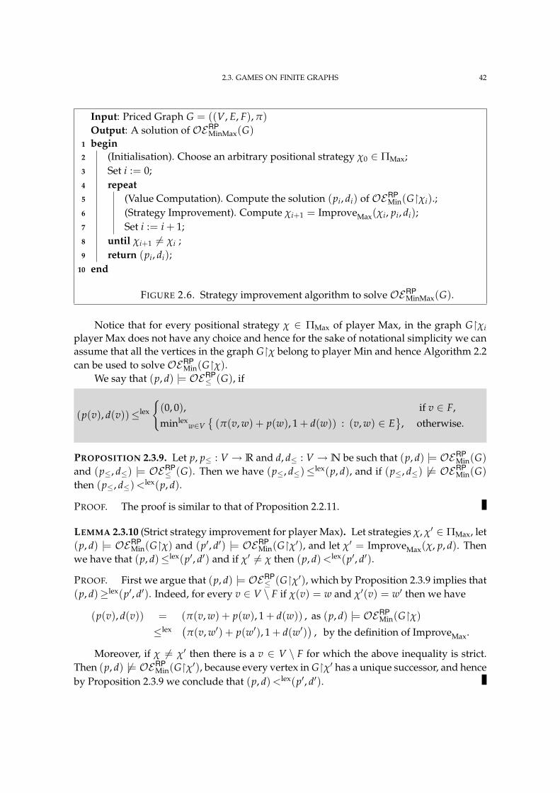
2.3. GAMES ON FINITE GRAPHS 42
Input: Priced Graph G = ((V, E, F), π)Output: A solution of OERP
MinMax(G)begin1
(Initialisation). Choose an arbitrary positional strategy χ0 ∈ ΠMax;2
Set i := 0;3
repeat4
(Value Computation). Compute the solution (pi, di) of OERPMin(Gχi).;5
(Strategy Improvement). Compute χi+1 = ImproveMax(χi, pi, di);6
Set i := i + 1;7
until χi+1 6= χi ;8
return (pi, di);9
end10
FIGURE 2.6. Strategy improvement algorithm to solve OERPMinMax(G).
Notice that for every positional strategy χ ∈ ΠMax of player Max, in the graph Gχiplayer Max does not have any choice and hence for the sake of notational simplicity we canassume that all the vertices in the graph Gχ belong to player Min and hence Algorithm 2.2can be used to solve OERP
Min(Gχ).We say that (p, d) |= OERP
≤ (G), if
(p(v), d(v))≤lex
(0, 0), if v ∈ F,
minlexw∈V
(π(v, w) + p(w), 1 + d(w)) : (v, w) ∈ E
, otherwise.
PROPOSITION 2.3.9. Let p, p≤ : V → R and d, d≤ : V →N be such that (p, d) |= OERPMin(G)
and (p≤, d≤) |= OERP≤ (G). Then we have (p≤, d≤)≤lex(p, d), and if (p≤, d≤) 6|= OERP
Min(G)then (p≤, d≤) <lex(p, d).
PROOF. The proof is similar to that of Proposition 2.2.11.
LEMMA 2.3.10 (Strict strategy improvement for player Max). Let strategies χ, χ′ ∈ ΠMax, let(p, d) |= OERP
Min(Gχ) and (p′, d′) |= OERPMin(Gχ′), and let χ′ = ImproveMax(χ, p, d). Then
we have that (p, d)≤lex(p′, d′) and if χ′ 6= χ then (p, d) <lex(p′, d′).
PROOF. First we argue that (p, d) |= OERP≤ (Gχ′), which by Proposition 2.3.9 implies that
(p, d)≥lex(p′, d′). Indeed, for every v ∈ V \ F if χ(v) = w and χ′(v) = w′ then we have
(p(v), d(v)) = (π(v, w) + p(w), 1 + d(w)) , as (p, d) |= OERPMin(Gχ)
≤lex (π(v, w′) + p(w′), 1 + d(w′)
), by the definition of ImproveMax.
Moreover, if χ 6= χ′ then there is a v ∈ V \ F for which the above inequality is strict.Then (p, d) 6|= OERP
Min(Gχ′), because every vertex in Gχ′ has a unique successor, and henceby Proposition 2.3.9 we conclude that (p, d) <lex(p′, d′).
2.3. GAMES ON FINITE GRAPHS 43
LEMMA 2.3.11 (Correctness and termination of strategy improvement algorithm). Thestrategy improvement algorithm forOERP
MinMax terminates in finitely many steps and returnsa solution (p, d) of OERP
MinMax.
2.3.2. Solving Discounted-price Games
2.3.2.1. Optimality Equations
To solve a discounted-price game (Γ, DPMin(λ), DPMax(λ)) with a discount factor λ ∈ (0, 1),let us consider the following set of optimality equations.
D(v) =
min(v,w)∈E
(1− λ) · π(v, w) + λ · D(w)
, if v ∈ VMin,
max(v,w)∈E(1− λ) · π(v, w) + λ · D(w)
, if v ∈ VMax.
We denote these equations by OEDPMinMax(G, λ). We say that a functions d : V → R is a
solution of optimality equations OEDPMinMax(G, λ), and we write d |= OEDP
MinMax(G, λ), if allequations in OEDP
MinMax(G, λ) hold for the valuations D(v) 7→ d(v).The following lemma states the relation between a solution of optimality equations and
the value of the discounted-price game on a priced graph.
LEMMA 2.3.12 (A solution of optimality equations gives value of the game). If d : V → R isa solution of OEDP
MinMax(G, λ) then for all v ∈ V we have that d(v) = Val(v).
PROPOSITION 2.3.13 (A solution of optimality equations gives positional optimal strategiesfor both players). For a priced graph G and discount factor λ ∈ (0, 1), if there exists asolution of OEDP
MinMax(G, λ) then both players have positional optimal strategies.
2.3.2.2. Existence of a solution
LEMMA 2.3.14 (Existence of a solution). For every priced graph G and discount factor λ ∈(0, 1), there exists a solution of the optimality equations OEDP
MinMax(G, λ).
We prove this lemma using the following strategy improvement algorithm, whichterminates with a solution of the optimality equations.
2.3.2.3. Solving 2-player Optimality Equations
For given function d : V → R, let us define the set M∗(v, d) for every vertex v ∈ V asfollows:
M∗(v, d) = argmaxw∈V
(1− λ) · π(v, w) + λ · d(w) : (v, w) ∈ E.
Consider the strategy improvement function ImproveMax : ΠMax × [V → R] → ΠMaxdefined by:
ImproveMax(χ, d)(v) =
χ(v) if χ(v) ∈ M∗(v, d)Choose(M∗(v, d)) otherwise.
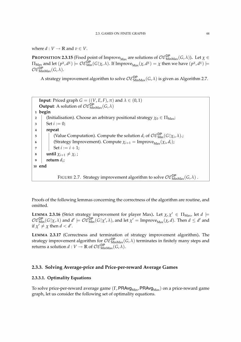
2.3. GAMES ON FINITE GRAPHS 44
where d : V → R and v ∈ V.
PROPOSITION 2.3.15 (Fixed point of ImproveMax are solutions of OEDPMinMax(G, λ)). Let χ ∈
ΠMax and let (pχ, dχ) |= OEDPMin(Gχ, λ). If ImproveMax(χ, dχ) = χ then we have (pχ, dχ) |=
OEDPMinMax(G, λ).
A strategy improvement algorithm to solve OEDPMinMax(G, λ) is given as Algorithm 2.7.
Input: Priced graph G = ((V, E, F), π) and λ ∈ (0, 1)Output: A solution of OEDP
MinMax(G, λ)begin1
(Initialisation). Choose an arbitrary positional strategy χ0 ∈ ΠMax;2
Set i := 0;3
repeat4
(Value Computation). Compute the solution di of OEDPMin(Gχi, λ).;5
(Strategy Improvement). Compute χi+1 = ImproveMax(χi, di);6
Set i := i + 1;7
until χi+1 6= χi ;8
return di;9
end10
FIGURE 2.7. Strategy improvement algorithm to solve OEDPMinMax(G, λ) .
Proofs of the following lemmas concerning the correctness of the algorithm are routine, andomitted.
LEMMA 2.3.16 (Strict strategy improvement for player Max). Let χ, χ′ ∈ ΠMax, let d |=OEDP
Min(Gχ, λ) and d′ |= OEDPMin(Gχ′, λ), and let χ′ = ImproveMax(χ, d). Then d ≤ d′ and
if χ′ 6= χ then d < d′.
LEMMA 2.3.17 (Correctness and termination of strategy improvement algorithm). Thestrategy improvement algorithm for OEDP
MinMax(G, λ) terminates in finitely many steps andreturns a solution d : V → R of OEDP
MinMax(G, λ).
2.3.3. Solving Average-price and Price-per-reward Average Games
2.3.3.1. Optimality Equations
To solve price-per-reward average game (Γ, PRAvgMin, PRAvgMax) on a price-reward gamegraph, let us consider the following set of optimality equations.
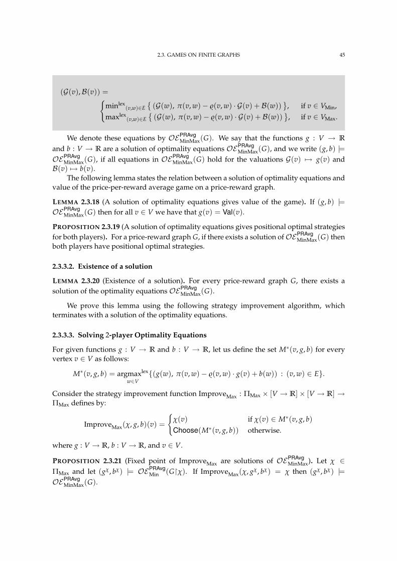
2.3. GAMES ON FINITE GRAPHS 45
(G(v),B(v)) =minlex
(v,w)∈E
(G(w), π(v, w)− $(v, w) · G(v) + B(w))
, if v ∈ VMin,
maxlex(v,w)∈E
(G(w), π(v, w)− $(v, w) · G(v) + B(w))
, if v ∈ VMax.
We denote these equations by OEPRAvgMinMax(G). We say that the functions g : V → R
and b : V → R are a solution of optimality equations OEPRAvgMinMax(G), and we write (g, b) |=
OEPRAvgMinMax(G), if all equations in OEPRAvg
MinMax(G) hold for the valuations G(v) 7→ g(v) andB(v) 7→ b(v).
The following lemma states the relation between a solution of optimality equations andvalue of the price-per-reward average game on a price-reward graph.
LEMMA 2.3.18 (A solution of optimality equations gives value of the game). If (g, b) |=OEPRAvg
MinMax(G) then for all v ∈ V we have that g(v) = Val(v).
PROPOSITION 2.3.19 (A solution of optimality equations gives positional optimal strategiesfor both players). For a price-reward graph G, if there exists a solution ofOEPRAvg
MinMax(G) thenboth players have positional optimal strategies.
2.3.3.2. Existence of a solution
LEMMA 2.3.20 (Existence of a solution). For every price-reward graph G, there exists asolution of the optimality equations OEPRAvg
MinMax(G).
We prove this lemma using the following strategy improvement algorithm, whichterminates with a solution of the optimality equations.
2.3.3.3. Solving 2-player Optimality Equations
For given functions g : V → R and b : V → R, let us define the set M∗(v, g, b) for everyvertex v ∈ V as follows:
M∗(v, g, b) = argmaxlex
w∈V(g(w), π(v, w)− $(v, w) · g(v) + b(w)) : (v, w) ∈ E.
Consider the strategy improvement function ImproveMax : ΠMax × [V → R]× [V → R] →ΠMax defines by:
ImproveMax(χ, g, b)(v) =
χ(v) if χ(v) ∈ M∗(v, g, b)Choose(M∗(v, g, b)) otherwise.
where g : V → R, b : V → R, and v ∈ V.
PROPOSITION 2.3.21 (Fixed point of ImproveMax are solutions of OEPRAvgMinMax). Let χ ∈
ΠMax and let (gχ, bχ) |= OEPRAvgMin (Gχ). If ImproveMax(χ, gχ, bχ) = χ then (gχ, bχ) |=
OEPRAvgMinMax(G).
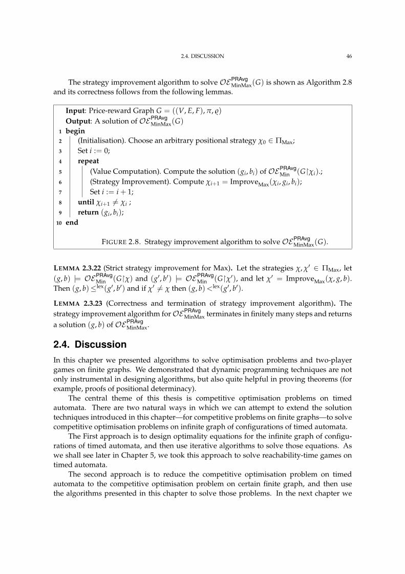
2.4. DISCUSSION 46
The strategy improvement algorithm to solve OEPRAvgMinMax(G) is shown as Algorithm 2.8
and its correctness follows from the following lemmas.
Input: Price-reward Graph G = ((V, E, F), π, $)Output: A solution of OEPRAvg
MinMax(G)begin1
(Initialisation). Choose an arbitrary positional strategy χ0 ∈ ΠMax;2
Set i := 0;3
repeat4
(Value Computation). Compute the solution (gi, bi) of OEPRAvgMin (Gχi).;5
(Strategy Improvement). Compute χi+1 = ImproveMax(χi, gi, bi);6
Set i := i + 1;7
until χi+1 6= χi ;8
return (gi, bi);9
end10
FIGURE 2.8. Strategy improvement algorithm to solve OEPRAvgMinMax(G).
LEMMA 2.3.22 (Strict strategy improvement for Max). Let the strategies χ, χ′ ∈ ΠMax, let(g, b) |= OEPRAvg
Min (Gχ) and (g′, b′) |= OEPRAvgMin (Gχ′), and let χ′ = ImproveMax(χ, g, b).
Then (g, b)≤lex(g′, b′) and if χ′ 6= χ then (g, b) <lex(g′, b′).
LEMMA 2.3.23 (Correctness and termination of strategy improvement algorithm). Thestrategy improvement algorithm forOEPRAvg
MinMax terminates in finitely many steps and returnsa solution (g, b) of OEPRAvg
MinMax.
2.4. DiscussionIn this chapter we presented algorithms to solve optimisation problems and two-playergames on finite graphs. We demonstrated that dynamic programming techniques are notonly instrumental in designing algorithms, but also quite helpful in proving theorems (forexample, proofs of positional determinacy).
The central theme of this thesis is competitive optimisation problems on timedautomata. There are two natural ways in which we can attempt to extend the solutiontechniques introduced in this chapter—for competitive problems on finite graphs—to solvecompetitive optimisation problems on infinite graph of configurations of timed automata.
The First approach is to design optimality equations for the infinite graph of configu-rations of timed automata, and then use iterative algorithms to solve those equations. Aswe shall see later in Chapter 5, we took this approach to solve reachability-time games ontimed automata.
The second approach is to reduce the competitive optimisation problem on timedautomata to the competitive optimisation problem on certain finite graph, and then usethe algorithms presented in this chapter to solve those problems. In the next chapter we
2.4. DISCUSSION 47
introduce boundary region graph, an abstraction of timed automata, which is quite usefulfor this purpose. In Chapter 4 we show that a number of optimisation problems on timedautomata can be reduced to corresponding optimisation problems on a finitary sub-graphof their boundary region graph. In Chapter 6 we show that the problem of solving average-time games on timed automata can be reduced to the problem of solving average pricegames on a finitary sub-graph of their boundary region graph.
3Timed Automata
For compositional reasoning, weshould be able to define thesemantics of a component andprove its properties withoutknowing the details of the otherparts of the system. Shifting todense-time semantics offers anatural and mathematicallyclean way to this effect.
Rajeev Alur
Mathematical formalisms to model real-time systems can broadly be divided in twocategories: discrete-time models and dense-timed models. In discrete-time models thevariables measuring time are (non-negative) integer-valued, while in dense-time modelsthe variables measuring time are (non-negative) real-valued. To model a real-time systemwith discrete-time models we are forced to fix a time-unit in advance and to ignore therelative order of two events within a unit of time. If we choose a small enough time-unitthen meaningful results can be obtained using discrete-time models. However, probably, thestrongest case against discrete-time models is that if a system is to be composed of severalcomponents, the semantics of each component can not be given independently. Dense-timemodels handles this issue elegantly as we are not required to fix a unit of time in advance.Timed automata [AD90] are dense-time computational models for real-time systems.
This chapter introduces timed automata and some of its extensions and sets notationsand mathematical shorthands that are used consistently in the rest of the thesis. This chapteralso introduces some abstractions—including a novel boundary region graph abstraction—of timed automata, which are useful in solving competitive optimisation problems on theinfinite graphs of configurations of timed automata. Before we present formal definitions oftimed automata, let us give two short examples of modelling real-time systems using timedautomata.
48
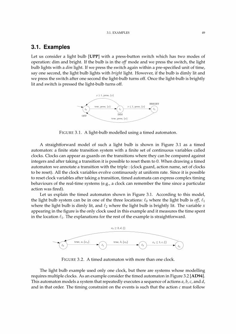
3.1. EXAMPLES 49
3.1. ExamplesLet us consider a light bulb [UPP] with a press-button switch which has two modes ofoperation: dim and bright. If the bulb is in the off mode and we press the switch, the lightbulb lights with a dim light. If we press the switch again within a pre-specified unit of time,say one second, the light bulb lights with bright light. However, if the bulb is dimly lit andwe press the switch after one second the light-bulb turns off. Once the light-bulb is brightlylit and switch is pressed the light-bulb turns off.
`1`0 `2true, press, x x ≤ 1, press, x
true, press, x
x ≥ 1, press, x
OFF DIM
BRIGHT
FIGURE 3.1. A light-bulb modelled using a timed automaton.
A straightforward model of such a light bulb is shown in Figure 3.1 as a timedautomaton: a finite state transition system with a finite set of continuous variables calledclocks. Clocks can appear as guards on the transitions where they can be compared againstintegers and after taking a transition it is possible to reset them to 0. When drawing a timedautomaton we annotate a transition with the triple : (clock guard, action name, set of clocksto be reset). All the clock variables evolve continuously at uniform rate. Since it is possibleto reset clock variables after taking a transition, timed automata can express complex timingbehaviours of the real-time systems (e.g., a clock can remember the time since a particularaction was fired).
Let us explain the timed automaton shown in Figure 3.1. According to this model,the light bulb system can be in one of the three locations: `0 where the light bulb is off, `1where the light bulb is dimly lit, and `2 where the light bulb is brightly lit. The variable xappearing in the figure is the only clock used in this example and it measures the time spentin the location `1. The explanations for the rest of the example is straightforward.
`1`0 `2 `3
true, a, xa true, b, xb xa ≤ 1, c,
xb ≥ 2, d,
FIGURE 3.2. A timed automaton with more than one clock.
The light bulb example used only one clock, but there are systems whose modellingrequires multiple clocks. As an example consider the timed automaton in Figure 3.2 [AD94].This automaton models a system that repeatedly executes a sequence of actions a, b, c, and d,and in that order. The timing constraint on the events is such that the action c must follow
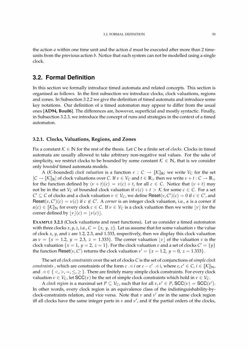
3.2. FORMAL DEFINITION 50
the action a within one time unit and the action d must be executed after more than 2 time-units from the previous action b. Notice that such system can not be modelled using a singleclock.
3.2. Formal Definition
In this section we formally introduce timed automata and related concepts. This section isorganised as follows. In the first subsection we introduce clocks, clock valuations, regionsand zones. In Subsection 3.2.2 we give the definition of timed automata and introduce somekey notations. Our definition of a timed automaton may appear to differ from the usualones [AD94, Bou06]. The differences are, however, superficial and mostly syntactic. Finally,in Subsection 3.2.3, we introduce the concept of runs and strategies in the context of a timedautomaton.
3.2.1. Clocks, Valuations, Regions, and Zones
Fix a constant K ∈N for the rest of the thesis. Let C be a finite set of clocks. Clocks in timedautomata are usually allowed to take arbitrary non-negative real values. For the sake ofsimplicity, we restrict clocks to be bounded by some constant K ∈ N, that is we consideronly bounded timed automata models.
A (K-bounded) clock valuation is a function ν : C → JKKR; we write VC for the set[C → JKKR] of clock valuations over C. If ν ∈ VC and t ∈ R⊕ then we write ν + t : C → R⊕for the function defined by (ν + t)(c) = ν(c) + t, for all c ∈ C. Notice that (ν + t) maynot be in the set VC of bounded clock valuation if ν(c) + t > K for some c ∈ C. For a setC′ ⊆ C of clocks and a clock valuation ν ∈ VC, we define Reset(ν, C′)(c) = 0 if c ∈ C′, andReset(ν, C′)(c) = ν(c) if c 6∈ C′. A corner is an integer clock valuation, i.e., α is a corner ifα(c) ∈ JKKN for every clock c ∈ C. If ν ∈ VC is a clock valuation then we write bνc for thecorner defined by bνc(c) = bν(c)c.EXAMPLE 3.2.1 (Clock valuations and reset functions). Let us consider a timed automatonwith three clocks x, y, z, i.e., C = x, y, z. Let us assume that for some valuation ν the valueof clock x, y, and z are 1.2, 2.3, and 1.333, respectively, then we display this clock valuationas ν = x = 1.2, y = 2.3, z = 1.333. The corner valuation bνc of the valuation ν is theclock valuation x = 1, y = 2, z = 1. For the clock valuation ν and a set of clocks C′ = ythe function Reset(ν, C′) returns the clock valuation ν′ = x = 1.2, y = 0, z = 1.333.
The set of clock constraints over the set of clocks C is the set of conjunctions of simple clockconstraints , which are constraints of the form c ./ i or c− c′ ./ i, where c, c′ ∈ C, i ∈ JKKN,and ./ ∈ <, >, =,≤,≥. There are finitely many simple clock constraints. For every clockvaluation ν ∈ VC, let SCC(ν) be the set of simple clock constraints which hold in ν ∈ VC.
A clock region is a maximal set P ⊆ VC, such that for all ν, ν′ ∈ P, SCC(ν) = SCC(ν′).In other words, every clock region is an equivalence class of the indistinguishability-by-clock-constraints relation, and vice versa. Note that ν and ν′ are in the same clock regioniff all clocks have the same integer parts in ν and ν′, and if the partial orders of the clocks,
3.2. FORMAL DEFINITION 51
Clock x
Clo
cky
0 1 20
1
2
P1 : 0 = y < x < 1
P2 : 0 < y < x < 1
P3 : 0 < y < x = 1
P0 : x = y = 0
FIGURE 3.3. Clock regions of a timed automaton.
determined by their fractional parts in ν and ν′, are the same. For all ν ∈ VC, we write [ν]for the clock region of ν.
EXAMPLE 3.2.2 (Clock regions). The set of the clock valuation with two clocks, x and y,and bound K = 2 is illustrated in Figure 3.3. Notice that all the intersection points (e.g.,clock region P0), open line segments (e.g., clock region P1 and P3), and open areas (e.g.,clock region P2) are different clock regions. Total number of regions in this example is 33 (9intersection points, 16 open line segments and 8 triangular open areas).
A clock zone is a convex set of clock valuations, which is a union of a set of clock regions.We write Z for the set of clock zones. Note that a set of clock valuations is a zone iff it isdefinable by a clock constraint. For W ⊆ VC, we write clos(W) for the smallest closed setin VC which contains W. Observe that for every clock zone W, the set clos(W) is also a clockzone.
Let L be a finite set of locations . A configuration is a pair (`, ν), where ` ∈ L is a locationand ν ∈ VC is a clock valuation; we write Q for the set of configurations. If s = (`, ν) ∈ Qand c ∈ C, then we write s(c) for ν(c).
A region is a pair (`, P), where ` is a location and P is a clock region. If s = (`, ν) is aconfiguration then we write [s] for the region (`, [ν]). A region R = (`, P) corresponds to aset of configurations (`, ν) : [ν] = P, hence sometimes we write s ∈ R as a shorthand for[s] = R. We write R for the set of regions. A set Z ⊆ Q is a zone if for every ` ∈ L, there isa clock zone W` (possibly empty), such that Z = (`, ν) : ` ∈ L and ν ∈ W`. For a regionR = (`, P) ∈ R, we write clos(R) for the zone (`, ν) : ν ∈ clos(P).
3.2.2. Timed Automata
We are now in a position to introduce a timed automaton.
3.2. FORMAL DEFINITION 52
DEFINITION 3.2.3 (Timed Automata). A timed automaton is a tuple T = (L, C, S, A, E, δ, ξ, F),where:
– L is a finite set of locations,– C is a finite set of clocks,– S ⊆ L× VC is a set of states 1,– A is a finite set of actions,– E : A→ 2S is an action enabledness function,– δ : L× A→ L is a transition function,– ξ : A→ 2C is a clock reset function, and– F ⊆ S is a set of final states.
It is required that S, F, and E(a) for all a ∈ A, are zones.
Clock zones, from which zones S, F, and E(a), for all a ∈ A, are built, are typicallyspecified by clock constraints. Therefore, when we consider a timed automaton as an inputof an algorithm, its size should be understood as the sum of sizes of encodings of L, C, A, δ,and ξ, and the sizes of encodings of clock constraints defining zones S, F, and E(a), for alla ∈ A.
Remark. In standard definitions [Alu91, Bou09] of timed automata, transitions are allowedto be non-deterministic, i.e., the transition function has the form δ : L× A → 2L. However,in our work timed automata are not used as formal language acceptors, but rather asgenerators of (classes of) transition systems. It is the game structure (i.e., the partition ofstates for the two players) that is in fact introducing two forms of non-deterministic choices,sometimes referred to, e.g., as “angelic” and “demonic” non-determinism. In this contextworking with “deterministic” automata is more meaningful because it does not introducean unnecessary “third” form of non-determinism. Since we never interpret automata asformal language acceptors, restriction to “deterministic” automata is hence without loss ofgenerality and avoids unnecessary confusion.
For a configuration s = (`, ν) ∈ Q and t ∈ R⊕, we define s + t to be the configurations′ = (`, ν + t) if ν + t ∈ VC, and we then write s −t s′. We write s −→t s′ if s −t s′ and forall t′ ∈ [0, t], we have (`, ν + t′) ∈ S. For an action a ∈ A, we define Succ(s, a) to be theconfiguration s′ = (`′, ν′), where `′ = δ(`, a) and ν′ = Reset(ν, ξ(a)), and we then writes a− s′. We write s a−→ s′ if s a− s′; s, s′ ∈ S; and s ∈ E(a).
ASSUMPTION 3.2.4. For technical convenience, and without loss of generality, we willassume throughout that for every s ∈ S, there exists a ∈ A, such that s a−→ s′.
For s, s′ ∈ S, we say that s′ is in the future of s, or equivalently, that s is in the past of s′,if there is t ∈ R⊕, such that s −→t s′; we then write s −→∗ s′.
1The set of states is usually specified as an invariant function [HNSY92] I : L → Z on the locations suchthat S =
(`, ν) : ν ∈ I(`)
.
3.3. SOME PROPERTIES OF REGIONS 53
3.2.3. Timed Actions, Runs, and Strategies
A timed action is a pair τ = (t, a) ∈ R⊕× A. For s ∈ Q, we define Succ(s, τ) = Succ(s, (t, a))to be the configuration s′ = Succ(s + t, a), i.e., such that s −t s′′ a− s′, and we then writes a−t s′. We write s a−→t s′ if s −→t s′′ a−→ s′, and we then say that (s, (t, a), s′) is a transitionof the timed automaton. If τ = (t, a) then we write s τ− s′ instead of s a−t s′, and s τ−→ s′
instead of s a−→t s′.A finite run of a timed automaton T is a sequence
〈s0, τ1, s1, τ2, . . . , τn, sn〉 ∈ S× ((R⊕ × A)× S)∗,
such that for every positive integer i ≤ n we have that (si−1, τi, si) is a transition, i.e.,si−1
τi−→ si. For a finite run r = 〈s0, τ1, s1, τ2, . . . , τn, sn〉 we define Length(r) = n and wedefine Last(r) = sn to be the state in which the run ends. We write Runsfin for the set offinite runs, and Runsfin(s) for the set of finite runs starting from state s ∈ S.
An infinite run of a timed automaton T is a sequence
〈s0, τ1, s1, τ2, . . .〉 ∈ S× ((R⊕ × A)× S)ω,
such that for all i ≥ 1, we have si−1τi−→ si. For an infinite run r, we define Length(r) = ∞.
For a run r = 〈s0, τ1, s1, τ2, . . .〉, we define Stop(r) = infi : si ∈ F. We write Runs for theset of infinite runs, and Runs(s) for the set of infinite runs starting from state s ∈ S. For arun r = 〈s0, τ1, s1, τ2, . . .〉, we define time of the run as Time(r) = ∑Length(r)
i=1 ti.A strategy is a function σ : Runsfin → R⊕× A, such that if Last(r) = s ∈ S and σ(r) = τ
then s τ−→ s′. We write Σ for the set of strategies. A run according to a strategy σ from a states ∈ S is the unique run Run(s, σ) = 〈s0, τ1, s1, τ2, . . .〉, such that s0 = s, and for every i ≥ 1,we have σ(Runi(s, σ)) = τi+1, where Runi(s, σ) = 〈s0, τ1, s1, . . . , si−1, τi, si〉.
We say that a strategy σ is positional if for all finite runs r, r′ ∈ Runsfin, we have thatLast(r) = Last(r′) implies σ(r) = σ(r′). A positional strategy can be then representedas a function σ : S → R⊕ × A, which uniquely determines the strategy σ∞ ∈ Σ asfollows: σ∞(r) = σ(Last(r)), for all finite runs r ∈ Runsfin. We write Π for the sets ofpositional strategies.
3.3. Some Properties of RegionsLet us recall that a clock region is an equivalence class of the indistinguishability-by-clock-constraints relation, while a region is a pair of a location and a clock region. We write Rfor the set of regions of a timed automaton T . In this section we discuss some propertiesof regions and we begin by defining fractional signature and cellular signature of a clockvaluation.
3.3.1. Fractional Signature and Cellular Signature
For a clock valuation ν we define its fractional signature HνI to be the sequence ( f0, f1, . . . , fm),such that f0 = 0, fi < f j if i < j, for all i, j ≤ m, and f1, f2, . . . , fm are all the non-zero
3.3. SOME PROPERTIES OF REGIONS 54
fractional parts of clock values in the clock valuation ν. In other words, for every i ≥ 1,there is a clock c, such that *ν(c)+ = fi, and for every clock c ∈ C, there is i ≤ m, such that*ν(c)+ = fi. Let ( f0, f1, . . . , fm) be the fractional signature HνI. Then the cellular signature LνMof a clock valuation ν is defined to be the partition (D0, D1, . . . , Dm) of the set C of clocks,such that Di = c ∈ C : *ν(c)+ = fi, for all i ≤ m. We then define Cell(ν, c) to be thenumber i such that c ∈ Di.
EXAMPLE 3.3.1 (fractional and cellular signatures). Let us consider clock valuations ν =x = 1.2, y = 2.3, z = 1.333 and ν′ = x = 1.2, y = 0, z = 1.333 from Example 3.2.1.The fractional signature of ν is HνI = (0, 0.2, 0.3, 0.333), and the fractional signature of ν′
is HνI = (0, 0.2, 0.333). The cellular signature of ν is LνM = (∅, x, y, z), while thecellular signature of ν′ is Lν′M = (y, x, z).
An equivalent definition of a clock region is given in terms of cellular signature: a clockregion is a pair (α, D), where α is a corner and D is a cellular signature. For a clock valuationν ∈ VC, we write [ν] for the clock region (bνc, LνM).
EXAMPLE 3.3.2. We can write the clock region of the clock valuation ν = x = 1.2, y =2.3, z = 1.333 as (x = 1, y = 2, z = 1, (∅, x, y, z)). Clock region P2 fromFigure 3.3 can be written as (x = 0, y = 0, (∅, y, x)), while the clock region P3 can bewritten as (x = 1, y = 0, (x, y)).
3.3.2. Thick and Thin Regions
For R, R′ ∈ R, we say that R′ is in the future of R, or that R is in the past of R′, if for all s ∈ R,there is s′ ∈ R′, such that s′ is in the future of s; we then write R −→∗ R′. We say that R′ is thetime successor of R if R −→∗ R′, R 6= R′, and for every R′′ ∈ R, we have that R −→∗ R′′ −→∗ R′
implies R′′ = R or R′′ = R′; we then write R −→+1 R′ or R′ ←−+1 R. Similarly, for R, R′ ∈ R,we write R a−→ R′ if there is s ∈ R, and there is s′ ∈ R′, such that s a−→ s′.
We say that a region R ∈ R is thin if for every s ∈ R and every ε > 0, we have that[s] 6= [s + ε]; other regions are called thick. We writeRThin andRThick for the sets of thin andthick regions, respectively. Note that if R ∈ RThick then for every s ∈ R, there is an ε > 0,such that [s] = [s + ε]. Observe also, that the time successor of a thin region is thick, andvice versa.
Another noteworthy property of a thin region is that for every thin region R ∈ RThinthere is a clock c ∈ C and a nonnegative integer b ∈ N+ such that for every state s ∈ Rwe have that s(c) = b. In other words if (D0, D1, . . . , Dm) is the cellular signature of a thinregion then D0 is nonempty.
EXAMPLE 3.3.3. Let ` be a location of a timed automaton with two clocks x and y and boundK = 2. The clock regions of this timed automaton are shown in Figure 3.3. The region(`, P2) and the region (`, P3) are in the future of the region (`, P1). The region (`, P2) is thetime successor of the region (`, P1), and the region (`, P3) is the time successor of the region(`, P2). The regions (`, P0), (`, P1) and (`, P3) are thin regions, while the region (`, P2) is athick region. Let us consider the regions (`, P1), (`, P2), and (`, P3) in their cellular signature
3.4. EXTENSIONS OF TIMED AUTOMATA 55
form:(`, P1) = (`, (x = 0, y = 0, (y, x))),
(`, P2) = (`, (x = 0, y = 0, (∅, y, x))), and
(`, P3) = (`, (x = 1, y = 0, (x, y))).
Notice how the corner and the cellular signature of a region changes as it evolves in time.
3.3.3. Time-Abstract Bisimulation
DEFINITION 3.3.4 (Time-Abstract Bisimulation [Bou09]). A relation B ⊆ S× S defined overthe set of states of a timed automata is a time-abstract bisimulation if for every pair of statess1, s2 ∈ S such that (s1, s2) ∈ B, for every nonnegative real number t1 ∈ R⊕, and everyaction a ∈ A such that s1
a−→t1 s′1, there exists a nonnegative real number t2 ∈ R⊕ such thats2
a−→t2 s′2 and (s′1, s′2) ∈ B.
Alur and Dill proved the following fact about the region equivalence relation.
LEMMA 3.3.5. [AD90] Region equivalence relation is a time-abstract bisimulation.
3.4. Extensions of Timed AutomataThe extensions of timed automata which are relevant to this thesis are priced timedautomata and timed game automata.
3.4.1. Priced Timed Automata
Priced timed automata are extensions of timed automata and are useful in modelling opti-mal budgeting and scheduling problems [BFH+01, BBL08, AM01] for real-time systems.
DEFINITION 3.4.1 (Priced Timed Automata). A priced timed automaton (T , π) consists ofa timed automaton T and a price function π : S × R⊕ × A → R. For every states ∈ S and every timed move (t, a) ∈ R⊕ × A, the price function π determines theprice π(s, t, a) of taking the timed move (t, a) from state s, i.e., the price of the transition(s, (t, a), Succ(s, (t, a))).
Linearly-priced timed automata [BFH+01], also known in the literature as weightedtimed automata [ALTP01, BBBR07, ABM04], augment timed automata with price informa-tion, such that the price of waiting in a location is proportional to the waiting time, hencethe name linearly-priced timed automata.
DEFINITION 3.4.2 (Linearly-Priced TA). A linearly-priced timed automaton (T , p) consists oftimed automaton T , and a price labelling function p : L ∪ A → R that assigns a price ratep(`) to every location ` ∈ L, and a price p(a) to every action a. A linearly-priced timedautomaton (T , p) is a priced timed automaton (T , π) such that for every state s = (`, ν)and every timed move (t, a) we have π(s, (t, a)) = p(`) · t + p(a).
3.4. EXTENSIONS OF TIMED AUTOMATA 56
Linearly-priced timed automata are useful in modelling scheduling problems of real-time systems where the price-per-time-unit curve of every resource in the system is linear,i.e., the price-rate of every resource is constant. In practice, however, price-per-time-unitcurve of resources can be non-linear—in particular convex or concave. Convex price-per-time-unit functions arise in the situations where price-rate of a resource is non-decreasingwith time (e.g. overtime labour), while concave price-per-time-unit functions arise if theprice-rate is non-increasing (e.g. price of hiring an equipment for a short duration). For adetailed discussion on the importance of convex and concave price functions in schedulingproblems, we refer the reader to Falk and Horowitz [FH72].
Since linearly-priced timed automata are inadequate to model such systems, we pro-pose generalisations of linearly-priced timed automata to concavely-priced and convexly-priced timed automata. Unlike for linearly-priced timed automata, we do not specifyexplicitly how the price function π : S×R⊕ × A is represented; for conceptual simplicityit is convenient to think of it as an oracle or a computational black box. For the definitionsand properties of concave functions and K-continuity (or Lipschitz-continuity with constantK), we refer the reader to Appendix B.
DEFINITION 3.4.3 (Concavely-Priced Timed Automata). A concavely-priced timed automaton(T , π, K) is a priced timed automaton (T , π) with a constant K > 0, such that for all actionsa ∈ A and for all regions R, R′ ∈ R, the function πa
R,R′ : (s, t) 7→ π(s, t, a) is concave andK-continuous2 on DR,R′ = (s, t) ∈ S×R⊕ : s ∈ R and (s + t) ∈ R′.
A convexly-priced timed automaton is defined in an analogous manner. Notice thatevery linearly-priced timed automaton is both a concavely-priced timed automaton anda convexly-priced timed automaton. To study price-per-reward optimisation, we need adual-priced timed automata, and for this purpose we define concave price-reward timedautomata.
DEFINITION 3.4.4 (Concave Price-Reward Timed Automata). A concave price-reward timedautomaton (T , π, $, K) is a timed automaton T with price and reward functions π, $ : S ×R⊕ × A → R, and a constant K > 0 such that for all actions a ∈ A and for all regionsR, R′ ∈ R, the functions (s, t) 7→ π(s, t, a) and (s, t) 7→ $(s, t, a) are K-continuous, andconcave and convex, respectively, on (s, t) ∈ S×R⊕ : s ∈ R and (s + t) ∈ R′.
We require the following assumption regarding the divergence of reward in a price-reward timed automaton.
ASSUMPTION 3.4.5 (Regional Non-Zenoness Assumption on Reward). A timed automatonis regionally non-Zeno 3 with respect to $, i.e., there exists a positive real number k such thatfor every run r = 〈s0, τ1, s1, τ2, . . . , τn, sn〉 ∈ Runsfin, with [s0] = [sn], (i.e., such that therun r forms a cycle in the finite region graph of the the timed automaton), we have that∑n
i=1 $(si−1, τi) ≥ k.
2If the timed automaton is bounded and πaR,R′ is concave, then such a K exists without loss of generality.
3This assumption is similar to the structural non-Zenoness assumption [Tri99]. While structural non-Zenoassumption concerns cycles of control graph of locations and transitions, regional non-Zeno assumption is lessrestrictive and requires non-Zeno rewards in cycles of region graph.
3.4. EXTENSIONS OF TIMED AUTOMATA 57
Such assumptions are standard for price-per-reward optimisation problems on finitegraphs (see Assumption 2.1.4) and timed automata (Bouyer et al. [BBL04]).
A convex price-reward timed automaton is defined in an analogous manner.In Chapter 4 we discuss minimisation problems on concavely-priced timed automata
and concave price-reward timed automata. The treatment for maximisation problems onconvexly-priced timed automaton and convex price-reward timed automata is similar andhence omitted.
3.4.2. Games on Timed Automata
Optimal controller synthesis of real-time open system (assuming adversarial environment)can be specified as two-player zero-sum games on timed automata. Broadly speaking, thereare two different ways to specify a game arena on a timed automaton: turn based games—specified by a partition of the set of locations between the two players, and concurrentgames—specified by a partition of the set of actions between the two players.
3.4.2.1. Turn Based Games
DEFINITION 3.4.6 (Timed Game Automata—Turn Based). A timed game automaton is a tupleΓ = (T , LMin, LMax), where:
– T = (L, C, S, A, E, δ, ξ, F) is a timed automaton,– LMin ⊆ L is the set of locations controlled by player Min, and– LMax ⊆ L is the set of locations controlled by player Max.
We require that the sets LMax and LMin form a partition of the set of locations L.
A play starts at a state s0 ∈ S. If s0 ∈ Lp, for p ∈ Max, Min , then player p chooses avalid timed move (t1, a1) and s1 = Succ(s0, (t1, a1)) becomes the new current state. Whenthis happens then we say that player p has made a timed move from the current state.Players keep making timed moves in this way indefinitely, thus forming an infinite runr = 〈s0, τ1s1, τ2, . . .〉 of the timed automaton.
A strategy for Min is a function µ : Runsfin → A×R⊕, such that if Last(r) = s ∈ SMin
and µ(r) = τ then s τ−→ s′, where s′ = Succ(s, τ). Similarly, a strategy for player Max is afunction χ : Runsfin → A×R⊕, such that if Last(r) = s ∈ SMax and χ(r) = τ then s τ−→ s′,where s′ = Succ(s, τ). We write ΣMin for the set of strategies for player Min, and we writeΣMax for the set of strategies for player Max.
If players Min and Max use strategies µ and χ, resp., then the (µ, χ)-run from a state sis the unique run Run(s, µ, χ) = 〈s0, τ1, s1, τ2, . . .〉, such that s0 = s, and for every i ≥ 1, ifsi ∈ SMin, or si ∈ SMax, then µ(Runi(s, µ, χ)) = τi+1, or χ(Runi(s, µ, χ)) = τi+1, resp., whereRuni(s, µ, χ) = 〈s0, τ1, s1, . . . , si−1, τi, si〉.
We say that a strategy µ for Min is positional if for all finite runs r, r′ ∈ Runsfin, wehave that Last(r) = Last(r′) implies µ(r) = µ(r′). A positional strategy for player Mincan be then represented as a function µ : SMin → A×R⊕, which uniquely determines thestrategy µ∞ ∈ ΣMin as follows: µ∞(r) = µ(Last(r)), for all finite runs r ∈ Runsfin. Positional
3.4. EXTENSIONS OF TIMED AUTOMATA 58
strategies for player Max are defined and represented in the analogous way. We write ΠMinand ΠMax for the sets of positional strategies for player Min and for player Max, respectively.
3.4.2.2. Concurrent Games
Minor variants of the following timed game automata are considered in literature [AM99,BHPR07, ABM04].
DEFINITION 3.4.7 (Timed Game Automata [AM99]—Concurrent Games). A timed gameautomaton is a tuple (L, C, S, AMin, AMax, ε, E, δ, ξ, F), where
– L is a finite set of locations,– C is a finite set of clocks,– S ⊆ L× VC is a set of states,– AMin is a finite set actions controlled by player Min,– AMax is a finite set actions controlled by player Max,– ε is a special empty action,– E : AMin ∪ AMax → 2S is an action enabledness function,– δ : L× Aε
Min × AεMax → L is a transition function,
– ξ : AεMin × Aε
Max → 2C is a clock reset function, and– F ⊆ S is a set of final states.
Here AεMin and Aε
Max stand for AMin ∪ ε and AMax ∪ ε, respectively. It is required thatS, F, and E(a) for all a ∈ A, are zones.
Starting from some state s0 ∈ S both players choose timed moves τn ∈ R⊕ × AMin andτx ∈ R⊕ × AMax simultaneously; the next state of the system is determined by their jointaction and is given by the successor function Succ : S×R⊕ × AMin ×R⊕ × AMax → S inthe following manner:
Succ((`, ν), (tn, an), (tx, ax)) =
(δ(`, an, ε), Reset(ν + tn, ξ(an, ε))) if tn < tx
(δ(`, ε, ax), Reset(ν + tx, ξ(ε, ax))) if tx < tn
(δ(`, an, ax), Reset(ν + t, ξ(an, ax))) if t = tx = tn.
The play then evolves to the resulting state and the players continue to play indefinitelyto form an infinite run of the timed automaton. The strategies for the players can be definedin a straightforward manner.
3.4.2.3. A Case for Turn-based Games
Arguably, concurrent games can be used to model a larger class of open real-time systemsthan turn based games. However, in this thesis, we focus our attention to turn-based games.Turn based games are simple to analyse using dynamic programming techniques, and area good first step in establishing effective techniques for solving competitive optimisationon timed automata. Another reason for choosing the turn-based model is that concurrentgames on timed automata often lack determinacy (see, e.g., de Alfaro et al. [dAFH+03]).
3.5. COMPETITIVE OPTIMISATION ON TIMED AUTOMATA 59
3.5. Competitive Optimisation on Timed AutomataIn this section we define competitive optimisation problems on timed automata which areof interest in this thesis. Since some of these problems are known by different names in theliterature, in this section we set a uniform terminology for these problems.
3.5.1. The Noncompetitive Case
In this thesis we consider minimisation problems for various cost functions on concavely-priced timed automata. Henceforth we reserve the term optimisation, optimum, andoptimal to refer to minimisation, minimum, and minimal, respectively. Fix a timedautomaton T , price and reward functions π, $ : S × R⊕ × A → R, and an initial states ∈ S.
A cost function is a function which takes an infinite run and returns its cost. Given acost function Cost : Runs → R we define the optimal cost function Cost∗ : S → R in thefollowing way:
Cost∗(s) = infr∈Runs(s)
Cost(r)
= inf
σ∈Σ
Cost(Run(s, σ))
.
The optimisation problem for the cost function Cost is to compute the optimum cost Cost∗(s)of a given state s ∈ S. The decision version of the optimisation problem is as follows: “givena timed automaton T , a state s ∈ S and a number D ∈ Q, determine whether Cost∗(s) ≤ D.”
We say that a strategy σ∗ ∈ Σ is optimal for the cost function Cost if we have thatCost(Run(s, σ∗)) = Cost∗(s). For a given ε > 0, we say that a strategy σ ∈ Σ is ε-optimal ifwe have that Cost(Run(s, σ)) ≤ Cost∗(s) + ε.
Let r = 〈s0, τ1, s1, τ2, . . .〉 ∈ Runs be a run of the timed automaton T , where τi = (ti, ai)for every positive integer i. Moreover, for π and $, the price and reward functions,respectively, of a priced (or price-reward) timed automaton, and for every positive integer n,we define: Tn(r) = ∑n
i=1 ti, πn(r) = ∑ni=1 π(si−1, τi), and $n(r) = ∑n
i=1 $(si−1, τi).The following list of cost functions gives rise to a number of corresponding optimisa-
tion problems.(1) Reachability time. The reachability-time cost function is defined in the following
way: for every run r ∈ Runs we have
RT(r) =
TN(r), if N = Stop(r) < ∞,
∞, otherwise.
(2) Reachability price. The reachability-price cost function is defined in the followingway: for every run r ∈ Runs we have
RP(r) =
πN(r), if N = Stop(r) < ∞,
∞, otherwise.
(3) Discounted time. The discounted-time cost function is defined in the followingway: for every run r ∈ Runs and every discount factor λ ∈ (0, 1) we have
DT(λ)(r) = (1− λ)∞
∑i=1
λi−1ti.
3.5. COMPETITIVE OPTIMISATION ON TIMED AUTOMATA 60
(4) Discounted price. The discounted-price cost function is defined in the followingway: for every run r ∈ Runs and every discount factor λ ∈ (0, 1) we have
DP(λ)(r) = (1− λ)∞
∑i=1
λi−1π(si−1, τi).
(5) Average time. The average-time cost function is defined in the following way: forevery run r ∈ Runs we have
AT(r) = lim supn→∞
Tn
n.
(6) Average price. The average-price cost function is defined in the following way: forevery run r ∈ Runs we have
AP(r) = lim supn→∞
πn(r)n
.
(7) Price-per-time average. The price-per-time average cost function is defined in thefollowing way: for every run r ∈ Runs we have
PTAvg(r) = lim supn→∞
πn(r)Tn(r)
.
(8) Price-per-reward average. The price-per-reward average cost function is defined inthe following way: for every run r ∈ Runs we have
PRAvg(r) = lim supn→∞
πn(r)$n(r)
.
In Chapter 4 we show (Theorem 4.2.1) that for arbitrary initial state s ∈ S, theoptimisation problem for all these cost functions on a concavely-price timed automata orconcave price-reward timed automata, as appropriate, is PSPACE-complete.
3.5.2. Competitive Optimisation
Fix a timed game automaton Γ = (T , LMin, LMax), price and reward functions π, $ : S ×R⊕ × A→ R, and an initial state s ∈ S. Let ΣMin and ΣMax be the set of strategies for playerMin and player Max, respectively. In the context of games we sometimes refer to a run as aplay of the game.
DEFINITION 3.5.1 (Cost Game on a Timed Game Automaton). A cost game on a timed gameautomaton is a tuple (Γ, CostMin, CostMax), where:
– Γ = (T , LMin, LMax) is a timed game automaton,– CostMin : Runs → R is a payoff function for player Min which gives the amount
Min loses in a play, and– CostMax : Runs→ R is the payoff function for player Max, which gives the amount
Max wins in a play.
3.5. COMPETITIVE OPTIMISATION ON TIMED AUTOMATA 61
A cost game is called zero-sum if we have that CostMin(r) = CostMax(r) for every play rof the game.
Payoff functions CostMax : Runs → R and CostMin : Runs → R naturally gives rise tothe payoff functions CostMax : S× ΣMin × ΣMax → R and CostMin : S× ΣMin × ΣMax → R
in the following way: for strategies µ ∈ ΣMin and χ ∈ ΣMax of respective players anda state s ∈ S we have CostMin(s, µ, χ) = CostMin(Run(s, µ, χ)) and CostMax(s, µ, χ) =CostMax(Run(s, µ, χ)).
The upper value of a cost game at the state s is defined as the maximum loss that playerMin can secure, in a play starting at the state s, irrespective of the strategies used by playerMax. Similarly the lower value of a cost game at the state s is defined as the minimum winthat player Max can secure, in a play starting at the state s, irrespective of the strategies usedby player Min. Formally we define the upper value Val
Γ(s) and the lower-value ValΓ(s) of
the game at the state s by as follows:
ValΓ(s) = inf
µ∈ΣMinsup
χ∈ΣMax
CostMin(s, µ, χ), and ValΓ(s) = supχ∈ΣMax
infµ∈ΣMin
CostMax(s, µ, χ).
From Proposition 1.2.4 we know that the lower value of a game at a state is alwaysless than the upper value of the game at that state, i.e., for every state s ∈ S the inequalityValΓ(s) ≤ Val
Γ(s) always holds.
A cost game is determined if for every state s ∈ S, we have ValΓ(s) = ValΓ(s). We then
say that the value of the game exists. We write ValΓ(s) for this number and we call it thevalue of the game at the state s.
The strategies µ∗ ∈ ΣMin and χ∗ ∈ ΣMax are optimal for the respective players, if forevery state s ∈ S we have that
supχ∈ΣMax
CostMin(s, µ∗, χ) = ValΓ(s), and inf
µ∈ΣMinCostMin(s, µ∗, χ) = ValΓ(s).
We say that a game is positionally determined if players have positional optimal strate-gies.
If the game is determined then the competitive optimisation problem is to computevalue of the game Val(s) for a give state s ∈ S. The corresponding decision problem is givena cost game (Γ, CostMin, CostMax), a state s ∈ S and a number D ∈ Q, determine whetherValΓ(s) ≤ D.
The following cost games on timed automata are of interest.(1) Reachability game. A reachability game (Γ, ReachMin, ReachMax) has the following
payoff functions:
ReachMin(r) = ReachMax(r) =
N if N = Stop(r) < ∞∞ otherwise.
(2) Reachability-time game. A reachability-time game (Γ, RTMin, RTMax) has the follow-ing payoff functions:
RTMin(r) = RTMax(r) =
TN(r) if N = Stop(r) < ∞∞ otherwise.

3.5. COMPETITIVE OPTIMISATION ON TIMED AUTOMATA 62
(3) Reachability-price game. A reachability-price game (Γ, RPMin, RPMax) has the follow-ing payoff functions:
RPMin(r) = RPMax(r) =
πN(r) if N = Stop(r) < ∞∞ otherwise.
(4) Discounted-time game. For a given discount factor λ ∈ (0, 1), a discounted-timegame (Γ, DTMin(λ), DTMax(λ)) has the following payoff functions:
DTMin(λ)(r) = DTMax(λ)(r) = (1− λ)∞
∑i=1
λi−1ti.
(5) Discounted-price game. For a given discount factor λ ∈ (0, 1), a discounted-pricegame (Γ, DPMin(λ), DPMax(λ)) has the following payoff functions:
DPMin(λ)(r) = DPMax(λ)(r) = (1− λ)∞
∑i=1
λi−1π(si−1, τi).
(6) Average-time game. An average-time game (Γ, APMin, APMax) has the followingpayoff functions:
ATMin(r) = lim supn→∞
Tn(r)n
and ATMax(r) = lim infn→∞
Tn(r)n
.
(7) Average-price game. An average-price game (Γ, APMin, APMax) has the followingpayoff functions:
APMin(r) = lim supn→∞
πn(r)n
and APMax(r) = lim infn→∞
πn(r)n
.
(8) Price-per-time average game. In a similar manner, a price-per-time average game(Γ, PTAvgMin, PTAvgMax) has the following payoff functions:
PTAvgMin(r) = lim supn→∞
πn(r)Tn(r)
and PTAvgMax(r) = lim infn→∞
πn(r)Tn(r)
.
(9) Price-per-reward average game. In a similar manner, a price-per-reward average game(Γ, PRAvgMin, PRAvgMax) has the following payoff functions:
PRAvgMin(r) = lim supn→∞
πn(r)$n(r)
and PRAvgMax(r) = lim infn→∞
πn(r)$n(r)
.
In this thesis we study reachability-time games and average-time games in Chapter 5and Chapter 6, respectively, and show that these game are determined (Theorem 5.1.2and Theorem 6.4.2). We also prove that decision problems corresponding to these gamesare EXPTIME-complete for timed automata with at least two clocks (Theorem 5.5.4 andTheorem 6.5.1).
Reachability games were shown to be EXPTIME-complete for timed automata byHenzinger and Kopke [HK99]. In Chapter 5 we strengthen this results by showingthat reachability games are EXPTIME-hard for timed automata with at least two clocks(Theorem 5.5.3).
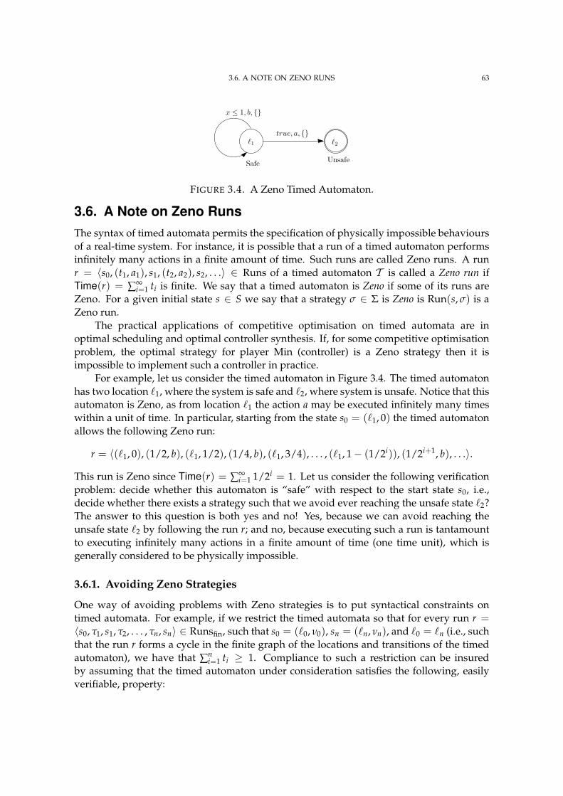
3.6. A NOTE ON ZENO RUNS 63
`1 `2
x ≤ 1, b,
true, a,
Safe Unsafe
FIGURE 3.4. A Zeno Timed Automaton.
3.6. A Note on Zeno RunsThe syntax of timed automata permits the specification of physically impossible behavioursof a real-time system. For instance, it is possible that a run of a timed automaton performsinfinitely many actions in a finite amount of time. Such runs are called Zeno runs. A runr = 〈s0, (t1, a1), s1, (t2, a2), s2, . . .〉 ∈ Runs of a timed automaton T is called a Zeno run ifTime(r) = ∑∞
i=1 ti is finite. We say that a timed automaton is Zeno if some of its runs areZeno. For a given initial state s ∈ S we say that a strategy σ ∈ Σ is Zeno is Run(s, σ) is aZeno run.
The practical applications of competitive optimisation on timed automata are inoptimal scheduling and optimal controller synthesis. If, for some competitive optimisationproblem, the optimal strategy for player Min (controller) is a Zeno strategy then it isimpossible to implement such a controller in practice.
For example, let us consider the timed automaton in Figure 3.4. The timed automatonhas two location `1, where the system is safe and `2, where system is unsafe. Notice that thisautomaton is Zeno, as from location `1 the action a may be executed infinitely many timeswithin a unit of time. In particular, starting from the state s0 = (`1, 0) the timed automatonallows the following Zeno run:
r = 〈(`1, 0), (1/2, b), (`1, 1/2), (1/4, b), (`1, 3/4), . . . , (`1, 1− (1/2i)), (1/2i+1, b), . . .〉.
This run is Zeno since Time(r) = ∑∞i=1 1/2i = 1. Let us consider the following verification
problem: decide whether this automaton is “safe” with respect to the start state s0, i.e.,decide whether there exists a strategy such that we avoid ever reaching the unsafe state `2?The answer to this question is both yes and no! Yes, because we can avoid reaching theunsafe state `2 by following the run r; and no, because executing such a run is tantamountto executing infinitely many actions in a finite amount of time (one time unit), which isgenerally considered to be physically impossible.
3.6.1. Avoiding Zeno Strategies
One way of avoiding problems with Zeno strategies is to put syntactical constraints ontimed automata. For example, if we restrict the timed automata so that for every run r =〈s0, τ1, s1, τ2, . . . , τn, sn〉 ∈ Runsfin, such that s0 = (`0, ν0), sn = (`n, νn), and `0 = `n (i.e., suchthat the run r forms a cycle in the finite graph of the locations and transitions of the timedautomaton), we have that ∑n
i=1 ti ≥ 1. Compliance to such a restriction can be insuredby assuming that the timed automaton under consideration satisfies the following, easilyverifiable, property:
3.7. ABSTRACTIONS OF TIMED AUTOMATA 64
DEFINITION 3.6.1 (Structural Non-Zenoness Assumption [BGS00]). A timed automaton isstructurally non-Zeno if in every cycle in the finite graph of locations and transitions at leastone clock is reset, and it is tested against some positive lower bound.
Asarin and Maler [AM99] used this assumption to solve reachability-time games ontimed automata. Another related assumption that appears in some publications [Tri99] isstrong non-Zenoness assumption, which states that every cycle in the control graph of timedautomata “spends” time. Note that structural non-Zenoness implies strong non-Zenoness.
Another way to avoid implementation issues with Zeno strategies is to forbid [MPS95]the controller (or the player Min) to use Zeno strategies, while the environment (or playerMax) can use Zeno strategies to its advantage. Such restrictions, however, may result insub-optimal strategies.
Henzinger et al. [dAFH+03, BHPR07] proposed an elegant way to handle the problemsof Zeno strategies by introducing timed games where players are penalised if they use Zenostrategies. In their work a player can win a game only by using the so-called receptivestrategies—strategies where the player is not responsible for a Zeno run. Unfortunatelyreceptive strategies can also be physically unimplementable. For instance consider astrategy which suggest to a player to take actions in the following time sequence (exampletaken from [CHR02]):
〈1, 112
, 2, 214
, 3, 318
, 4, 41
16, ...〉.
Notice that although this strategy is non-Zeno, it can be implemented only if the soft-ware/hardware with infinite precision is available. However, one can argue that if suchhardware/software is indeed available, even Zeno strategies are implementable.
In this thesis we do not require the timed automata to be non-Zeno. As a consequence,given a Zeno timed automaton as input, our algorithms may return unrealistic Zeno optimalstrategies for players. One related restriction (Assumption 3.4.5) is on the divergence ofreward function in price-reward timed automata. However, note that such an assumption(Assumption 2.1.4) on reward is required even for the weighted finite graphs.
3.7. Abstractions of Timed AutomataIn this section we review some abstractions of timed automata, and comment on theirsuitability to solve competitive optimisation problems.
3.7.1. Region Automata and Region Graphs
DEFINITION 3.7.1 (Region Automata [AD90]). The region automaton TRA = (R,M,RF) ofa timed automaton T is an edge-labelled finite graph with final vertices, where:
– the setR of regions of T is the set of vertices;– the labelled edge relationM⊆ R×R× A×R is defined by
M = (R, R′′, a, R′) : R −→∗ R′′ a−→ R′; and
– the set of final vertices RF ⊆ R is such that for every R ∈ RF we have that R ⊆ Fand for every R ∈ R \RF we have R ∩ F = ∅.
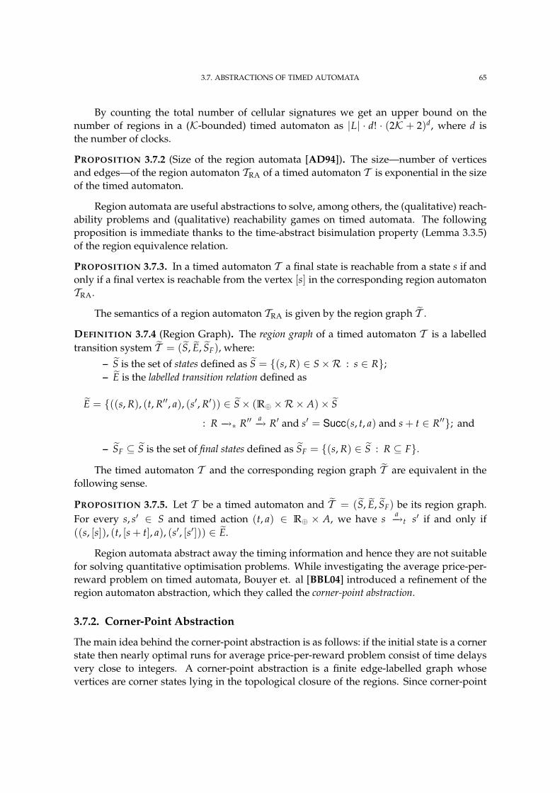
3.7. ABSTRACTIONS OF TIMED AUTOMATA 65
By counting the total number of cellular signatures we get an upper bound on thenumber of regions in a (K-bounded) timed automaton as |L| · d! · (2K + 2)d, where d isthe number of clocks.
PROPOSITION 3.7.2 (Size of the region automata [AD94]). The size—number of verticesand edges—of the region automaton TRA of a timed automaton T is exponential in the sizeof the timed automaton.
Region automata are useful abstractions to solve, among others, the (qualitative) reach-ability problems and (qualitative) reachability games on timed automata. The followingproposition is immediate thanks to the time-abstract bisimulation property (Lemma 3.3.5)of the region equivalence relation.
PROPOSITION 3.7.3. In a timed automaton T a final state is reachable from a state s if andonly if a final vertex is reachable from the vertex [s] in the corresponding region automatonTRA.
The semantics of a region automaton TRA is given by the region graph T .
DEFINITION 3.7.4 (Region Graph). The region graph of a timed automaton T is a labelledtransition system T = (S, E, SF), where:
– S is the set of states defined as S = (s, R) ∈ S×R : s ∈ R;– E is the labelled transition relation defined as
E = ((s, R), (t, R′′, a), (s′, R′)) ∈ S× (R⊕ ×R× A)× S
: R −→∗ R′′ a−→ R′ and s′ = Succ(s, t, a) and s + t ∈ R′′; and
– SF ⊆ S is the set of final states defined as SF = (s, R) ∈ S : R ⊆ F.
The timed automaton T and the corresponding region graph T are equivalent in thefollowing sense.
PROPOSITION 3.7.5. Let T be a timed automaton and T = (S, E, SF) be its region graph.For every s, s′ ∈ S and timed action (t, a) ∈ R⊕ × A, we have s a−→t s′ if and only if((s, [s]), (t, [s + t], a), (s′, [s′])) ∈ E.
Region automata abstract away the timing information and hence they are not suitablefor solving quantitative optimisation problems. While investigating the average price-per-reward problem on timed automata, Bouyer et. al [BBL04] introduced a refinement of theregion automaton abstraction, which they called the corner-point abstraction.
3.7.2. Corner-Point Abstraction
The main idea behind the corner-point abstraction is as follows: if the initial state is a cornerstate then nearly optimal runs for average price-per-reward problem consist of time delaysvery close to integers. A corner-point abstraction is a finite edge-labelled graph whosevertices are corner states lying in the topological closure of the regions. Since corner-point
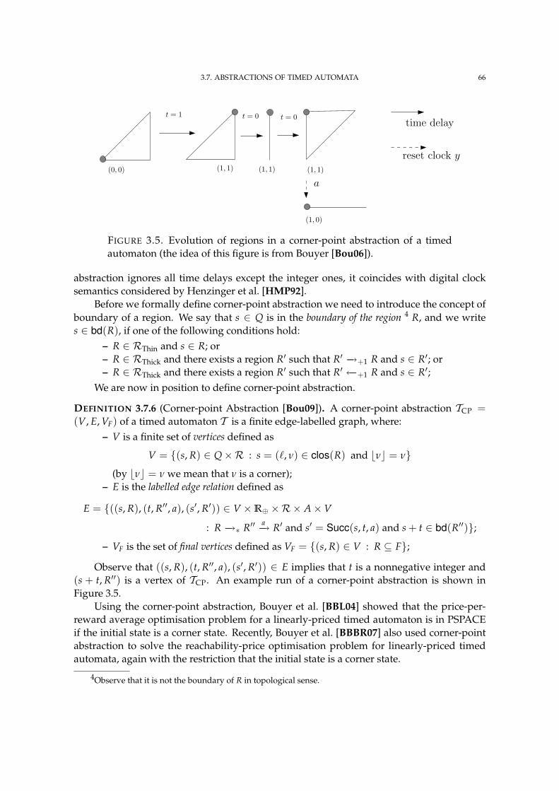
3.7. ABSTRACTIONS OF TIMED AUTOMATA 66
(0, 0) (1, 1) (1, 1)
(1, 0)
(1, 1)
t = 1 t = 0 t = 0
a
reset clock y
time delay
FIGURE 3.5. Evolution of regions in a corner-point abstraction of a timedautomaton (the idea of this figure is from Bouyer [Bou06]).
abstraction ignores all time delays except the integer ones, it coincides with digital clocksemantics considered by Henzinger et al. [HMP92].
Before we formally define corner-point abstraction we need to introduce the concept ofboundary of a region. We say that s ∈ Q is in the boundary of the region 4 R, and we writes ∈ bd(R), if one of the following conditions hold:
– R ∈ RThin and s ∈ R; or– R ∈ RThick and there exists a region R′ such that R′ −→+1 R and s ∈ R′; or– R ∈ RThick and there exists a region R′ such that R′ ←−+1 R and s ∈ R′;
We are now in position to define corner-point abstraction.
DEFINITION 3.7.6 (Corner-point Abstraction [Bou09]). A corner-point abstraction TCP =(V, E, VF) of a timed automaton T is a finite edge-labelled graph, where:
– V is a finite set of vertices defined as
V = (s, R) ∈ Q×R : s = (`, ν) ∈ clos(R) and bνc = ν(by bνc = ν we mean that ν is a corner);
– E is the labelled edge relation defined as
E = ((s, R), (t, R′′, a), (s′, R′)) ∈ V ×R⊕ ×R× A×V
: R −→∗ R′′ a−→ R′ and s′ = Succ(s, t, a) and s + t ∈ bd(R′′);– VF is the set of final vertices defined as VF = (s, R) ∈ V : R ⊆ F;
Observe that ((s, R), (t, R′′, a), (s′, R′)) ∈ E implies that t is a nonnegative integer and(s + t, R′′) is a vertex of TCP. An example run of a corner-point abstraction is shown inFigure 3.5.
Using the corner-point abstraction, Bouyer et al. [BBL04] showed that the price-per-reward average optimisation problem for a linearly-priced timed automaton is in PSPACEif the initial state is a corner state. Recently, Bouyer et al. [BBBR07] also used corner-pointabstraction to solve the reachability-price optimisation problem for linearly-priced timedautomata, again with the restriction that the initial state is a corner state.
4Observe that it is not the boundary of R in topological sense.
3.7. ABSTRACTIONS OF TIMED AUTOMATA 67
3.7.3. Boundary Region Automaton and Boundary Region Graph
Our original motivation for introducing the boundary region automaton was to solve thereachability price and price-per-reward average optimisation problems on linearly-pricedtimed automata with arbitrary initial states, i.e., including non-corner states. The assump-tion that nearly optimal runs for these two optimisation problems consist of time delays veryclose to nonnegative integers is incorrect if the initial state is a non-corner state. We observedthat if the initial state is an arbitrary state, a more general invariant holds— nearly optimalruns for these two optimisation problems consist of waiting until very close to the boundaryof some region before taking an action. We call such timed actions boundary timed actions andwe denote them by a triple (b, c, a) ∈ JKKN×C× A which represents the following symbolictimed action: take the action a when the value of clock c is “very close” to b.
DEFINITION 3.7.7 (Boundary Timed Actions). Define the finite set of boundary timed actionsA = JKKN × C× A. For s ∈ Q and α = (b, c, a) ∈ A, we define t(s, α) = b− s(c) if s(c) ≤ b,and t(s, α) = 0 if s(c) > b; and we define Succ(s, α) to be the state s′ = Succ(s, τ(α)), where
τ(α) = (t(s, α), a); we then write s α− s′. We also write s α−→ s′ if sτ(α)−−→ s′.
Note that if α ∈ A and s α−→ s′ then [s′] ∈ RThin. Observe that for every thin regionR′ ∈ RThin, there is a number b ∈ JKKN and a clock c ∈ C, such that for every R ∈ R in thepast of R′, we have that s ∈ R implies (s + (b− s(c)) ∈ R′; we then write R −→b,c R′. Forα = (a, b, c) ∈ A and R, R′ ∈ R, we write R α−→ R′ or R a−→b,c R′, if R −→b,c R′′ a−→ R′, for someR′′ ∈ RThin.
Boundary Region Automata. The motivation for the boundary region automata is thefollowing. Let a ∈ A, s = (`, ν) ∈ R and R→∗ R′ a−→ R′′.
– If R′ ∈ RThick, then there are infinitely many t ∈ R⊕ such that s+t ∈ R′. For allcompetitive optimisation problems solved in this thesis, one of the main results thatwe establish is that in the state s, amongst all such t’s, for one of the boundaries ofR′, the closer ν+t is to this boundary, the ‘better’ the timed action (t, a) becomesfor that problem. However, since R′ is a thick region, the set t ∈ R⊕ | s+t ∈ R′is an open interval, and hence does not contain its boundary values. Observe thatthe infimum equals binf−ν(cinf) where R →binf,cinf Rinf −→+1 R′ and the supremumequals bsup−ν(csup) where R →bsup,csup Rsup ←−+1 R′. In the boundary regionautomata, we include these ‘best’ timed action through the actions ((binf, cinf, a), R′)and ((bsup, csup, a), R′).
– If R′ ∈ RThin, then there exists a unique t ∈ R⊕ such that (`, ν+t) ∈ R′. Moreoversince R′ is a thin region there exists a clock c ∈ C and a number b ∈ N such thatR →b,c R′ and t = b−ν(c). In the boundary region automata we summarise this‘best’ timed action from region R via region R′ through the action ((b, c, a), R′).
With this intuition in mind, let us present the definition of a boundary region automata.
3.7. ABSTRACTIONS OF TIMED AUTOMATA 68
DEFINITION 3.7.8 (Boundary Region Automaton). The boundary region automaton TBR =(R,M,RF) of a timed automaton T is a finite edge-labelled graph with final vertices,where:
– the setR of regions of T is the set of vertices;– the labelled edge relation M ⊆ R×R×A×R is such that for every boundary timed
action α = (b, c, a) ∈ A and for all R, R′, R′′ ∈ R we have that (R, R′′, α, R′) ∈ M, ifand only if one of the following conditions holds—• R −→b,c R′′ a−→ R′, or• there is region R′′′ ∈ RThin such that R −→b,c R′′′ −→+1 R′′ a−→ R′, or• there is a region R′′′ ∈ RThin such that R −→b,c R′′′ ←−+1 R′′ a−→ R′;
– the set of final vertices RF ⊆ R is such that for every R ∈ RF we have that R ⊆ Fand for every R ∈ R \RF we have that R ∩ F = ∅.
The semantics of a boundary region automaton is given by the boundary region graph.
DEFINITION 3.7.9 (Boundary Region Graph). The boundary region graph T = (S, E, SF) of atimed automaton T is a labelled transition system, where:
– S is the set of states defined as
S = (s, R) ∈ Q×R : s ∈ clos(R);
– E is the labelled transition relation defined as
E = ((s, R), (t, R′′, a), (s′, R′)) ∈ S× (R⊕ ×R× A)× S
: R −→∗ R′′ a−→ R′ and s′ = Succ(s, t, a) and s + t ∈ bd(R′′); and
– SF is the set of final vertices defined as SF = (s, R) ∈ S : R ⊆ F.Boundary region graphs have the following property.
PROPOSITION 3.7.10. For every state in a boundary region graph T = (S, E, SF), the set ofreachable states is finite.
We prove Proposition 3.7.10 by constructing such reachable subgraph of a boundaryregion graph (Definition 3.7.12). Before we formally define the reachable subgraph of aboundary region graph from a certain state (s, R), we need to introduce some concepts.
The fractional signature of a a state (s, R) ∈ S of a boundary region graph is definedas *(s, R)+ = *ν+ where s = (`, ν). A state (s = (`, ν), R) of a boundary region graphis called a corner if its clock valuation ν is a corner. For a nonnegative integer k ≤ mwe define the k-shift of a fractional signature ( f0, f1, . . . , fm) as the fractional signature( f ′k, f ′k+1, . . . , f ′m, f ′0, . . . , f ′k−1) such that for all nonnegative integers i ≤ m we have f ′i =* fi + 1− fk+. We say that a fractional signature ( f ′0, f ′1, . . . , f ′n) is a subsequence of anotherfractional signature ( f0, f1, . . . , fm) if n ≤ m and for all nonnegative integers i < n we havef ′i ≤ f ′i+1; and for every nonnegative integer i ≤ n there exists a nonnegative integer j ≤ msuch that f ′i = f j.
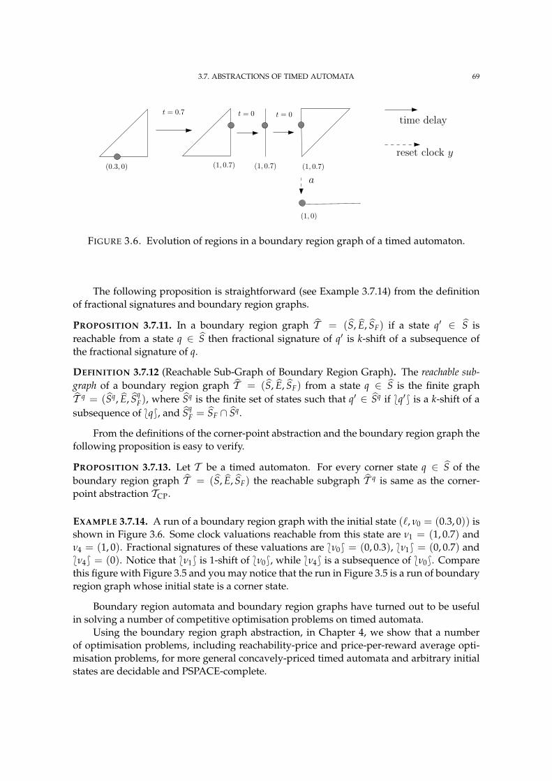
3.7. ABSTRACTIONS OF TIMED AUTOMATA 69
(0.3, 0) (1, 0.7) (1, 0.7)
(1, 0)
(1, 0.7)
t = 0.7 t = 0 t = 0
a
reset clock y
time delay
FIGURE 3.6. Evolution of regions in a boundary region graph of a timed automaton.
The following proposition is straightforward (see Example 3.7.14) from the definitionof fractional signatures and boundary region graphs.
PROPOSITION 3.7.11. In a boundary region graph T = (S, E, SF) if a state q′ ∈ S isreachable from a state q ∈ S then fractional signature of q′ is k-shift of a subsequence ofthe fractional signature of q.
DEFINITION 3.7.12 (Reachable Sub-Graph of Boundary Region Graph). The reachable sub-graph of a boundary region graph T = (S, E, SF) from a state q ∈ S is the finite graphT q = (Sq, E, Sq
F), where Sq is the finite set of states such that q′ ∈ Sq if *q′+ is a k-shift of asubsequence of *q+, and Sq
F = SF ∩ Sq.
From the definitions of the corner-point abstraction and the boundary region graph thefollowing proposition is easy to verify.
PROPOSITION 3.7.13. Let T be a timed automaton. For every corner state q ∈ S of theboundary region graph T = (S, E, SF) the reachable subgraph T q is same as the corner-point abstraction TCP.
EXAMPLE 3.7.14. A run of a boundary region graph with the initial state (`, ν0 = (0.3, 0)) isshown in Figure 3.6. Some clock valuations reachable from this state are ν1 = (1, 0.7) andν4 = (1, 0). Fractional signatures of these valuations are *ν0+ = (0, 0.3), *ν1+ = (0, 0.7) and*ν4+ = (0). Notice that *ν1+ is 1-shift of *ν0+, while *ν4+ is a subsequence of *ν0+. Comparethis figure with Figure 3.5 and you may notice that the run in Figure 3.5 is a run of boundaryregion graph whose initial state is a corner state.
Boundary region automata and boundary region graphs have turned out to be usefulin solving a number of competitive optimisation problems on timed automata.
Using the boundary region graph abstraction, in Chapter 4, we show that a numberof optimisation problems, including reachability-price and price-per-reward average opti-misation problems, for more general concavely-priced timed automata and arbitrary initialstates are decidable and PSPACE-complete.
3.7. ABSTRACTIONS OF TIMED AUTOMATA 70
In Chapter 5 we use boundary region automata to prove positional determinacy ofreachability-time games and we give an algorithm to solve reachability-time games bysolving reachability-time games on the corresponding boundary region automata.
In Chapter 6 we introduce another abstraction, called the closed region graph, whoseset of states is same as the set of states of corresponding boundary region graph, while thetransition relation is the union of the transition relations of the corresponding region graphand boundary region graph. We use closed region graphs to argue that, at every state of atimed automaton, the value of the average-time game is equal to the value of the average-time game, at a corresponding state, in its boundary region graph.
The definition of the boundary region automata and the boundary region graphsin these chapters are slightly modified to suit the problem under consideration. Thedifferences, however, are superficial.
Part 2
Competitive Optimisation on TimedAutomata
4Noncompetitive Optimisation
There is no opponent.
Bruce Lee
This chapter is dedicated to the study of noncompetitive optimisation problems ontimed automata. To cover a larger class of optimisation problems we work with concavely-priced timed automata, which are a generalisation of timed automata with price information.We consider minimisation problems for a variety of cost functions on concavely-pricedtimed automata in a uniform manner. For this purpose, we define the concept of concave-regularity of cost functions and show that minimisation problems for concave-regular costfunctions are PSPACE-complete for timed automata with at least three clocks. Finally, weshow that reachability time, reachability price, discounted time, discounted price, averagetime, average price, price-per-time average, and price-per-reward average cost functions areconcave-regular.
This chapter assumes familiarity with Lipschitz-continuous functions and their prop-erties, convex sets, concave and convex functions, quasiconcave and quasiconvex functions,and their properties. In Appendix B we give a short introduction to these concepts.
4.1. Concavely-Priced Timed AutomataLinearly-priced timed automata are extensions of timed automata with price information,and optimisation problems on linearly-priced timed automata are shown to be useful inmodelling optimal scheduling and budgeting problems [AM01, Bou06, BBL08] of real-time systems. For instance, consider a situation where we have to model an optimalscheduling problem using a timed automaton whose different locations correspond todifferent resources being consumed. If the price-per-time-unit of every resource is constantthen price function at every location is a linear function, and such a system can easily bemodelled using a linearly-priced timed automata. However, if the price-per-time-unit isincreasing or decreasing then linear prices are not adequate. To model such systems wepropose concavely-priced timed automata and convexly-priced timed automata; both aregeneralisations of linearly-priced timed automata.
A concavely-priced timed automaton (T , π, K) is a priced timed automaton (T , π) witha constant K > 0, such that for all actions a ∈ A and for all regions R, R′ ∈ R, the
72
4.2. OPTIMISATION PROBLEMS ON PRICED TIMED AUTOMATA 73
function πaR,R′ : (s, t) 7→ π(s, t, a) is concave and K-continuous on DR,R′ = (s, t) ∈
S × R⊕ : s ∈ R and (s + t) ∈ R′. A convexly-priced timed automaton is defined in ananalogous manner.
A concave price-reward timed automaton (T , π, $, K) is a timed automaton T with priceand reward functions π, $ : S × R⊕ × A → R, and a constant K > 0, such that forall actions a ∈ A and for all regions R, R′ ∈ R, the functions (s, t) 7→ π(s, t, a) and(s, t) 7→ $(s, t, a) are K-continuous, and concave and convex, respectively, on (s, t) ∈S × R⊕ : s ∈ R and (s + t) ∈ R′. A convex price-reward timed automaton is defined inan analogous manner. For technical convenience, we assume that the reward function isregionally non-Zeno (see Assumption 3.4.5).
In this chapter we only discuss minimisation problems on concavely-priced timedautomata and concave price-reward timed automata. The discussion on maximisationproblems on convexly-priced timed automata and convex price-reward timed automata isanalogous and has been omitted. Fix a timed automaton T (L, C, S, A, E, δ, ξ, F), price andreward functions π, $ : S×R⊕ × A→ R, and a constant K > 0.
4.2. Optimisation Problems on Priced Timed Automata
Let Cost : Runs → R be a cost function that for every run r ∈ Runs determines itscost Cost(r). We then define the minimum cost function Cost∗ : S→ R, by:
Cost∗(s) = infr∈Runs(s)
Cost(r)
= inf
σ∈Σ
Cost(Run(s, σ))
.
The minimisation problem for the cost function Cost is to compute the minimum cost Cost∗(s)for a given state s ∈ S. The decision version of the optimisation problem is as follows:“given a timed automaton T , a state s ∈ S and a number D ∈ Q, determine whetherCost∗(s) ≤ D.”
We say that a strategy σ∗ ∈ Σ is optimal for the cost function Cost if we have thatCost(Run(s, σ∗)) = Cost∗(s). For a given ε > 0, we say that a strategy σ ∈ Σ is ε-optimal ifwe have that Cost(Run(s, σ)) ≤ Cost∗(s) + ε.
Let r = 〈s0, τ1, s1, τ2, . . .〉 ∈ Runs be a run of the timed automaton T , where τi = (ti, ai)for every positive integer i. Moreover, for π and $, the price and reward functions,respectively, of a priced (or price-reward) timed automaton, and for every positive integer n,we define: Tn(r) = ∑n
i=1 ti, πn(r) = ∑ni=1 π(si−1, τi), and $n(r) = ∑n
i=1 $(si−1, τi).The following list of cost functions gives rise to a number of corresponding optimisa-
tion problems.
(1) Reachability price. The reachability-price cost function is defined in the followingway: for every run r ∈ Runs we have
RP(r) =
πN(r), if N = Stop(r) < ∞,
∞, otherwise.
4.3. REGION GRAPHS 74
(2) Discounted price. The discounted-price cost function is defined in the followingway: for every run r ∈ Runs and every discount factor λ ∈ (0, 1) we have
DP(λ)(r) = (1− λ)∞
∑i=1
λi−1π(si−1, τi).
(3) Average price. The average-price cost function is defined in the following way: forevery run r ∈ Runs we have
AP(r) = lim supn→∞
πn(r)n
.
(4) Price-per-time average. The price-per-time average cost function is defined in thefollowing way: for every run r ∈ Runs we have
PTAvg(r) = lim supn→∞
πn(r)Tn(r)
.
(5) Price-per-reward average. The price-per-reward average cost function is defined inthe following way: for every run r ∈ Runs we have
PRAvg(r) = lim supn→∞
πn(r)$n(r)
.
The following is the main result of the chapter:
THEOREM 4.2.1. The minimisation problems for reachability price, discounted price,average price, price-per-time average, and price-per-reward average cost functions, forconcavely-priced and concave price-reward timed automata, as appropriate, are PSPACE-complete.
The reachability problem for timed automata can be easily reduced, in logarithmicspace, to the minimisation problems discussed above so, by Theorem 1.3.1, they are allPSPACE-hard. In the following sections we prove that they are all in PSPACE, and hencewe establish the main Theorem 4.2.1.
The following sections are organised as follows. In Section 4.3 we revisit region graphT and boundary region graph T of a timed automaton T , and introduce a few notations.In Section 4.4 we introduce the concept of concave-regular cost functions, and prove thatminimisation problems on T for such cost functions can be reduced to correspondingminimisation problems on T . In Section 4.5 we show that reachability price, discountedprice, average price, price-per-time average, and price-per-reward average cost functionsare concave-regular.
4.3. Region GraphsFor the purpose of this chapter, we collectively refer to region graph and boundaryregion graph as region graphs. In Subsections 4.3.1 and 4.3.2 we introduce region graphand boundary region graph, respectively, of a concavely-priced timed automaton. InSubsection 4.3.3 we define reachability price, discounted price, average price, price-per-timeaverage, and price-per-reward average minimisation problems on these graph.
4.3. REGION GRAPHS 75
4.3.1. Region Graph
Let us recall the definition of the region graph of a timed automaton introduced in Chapter 3.The region graph of a timed automaton T = (L, C, S, A, E, δ, ξ, F) is a labelled transitionsystem T = (S, E, SF), where:
– S is the set of states defined as S = (s, R) ∈ S×R : s ∈ R;– E is the labelled transition relation defined as
E = ((s, R), (t, R′′, a), (s′, R′)) ∈ S× (R⊕ ×R× A)× S
: R −→∗ R′′ a−→ R′ and s′ = Succ(s, t, a) and s + t ∈ R′′; and
– SF ⊆ S is the set of final states defined as SF = (s, R) ∈ S : R ⊆ F.We say that
((s, R), (t, R′′, a), (s′, R′)
)is a transition in T = (S, E, SF) if we have that(
(s, R), (t, R′′, a), (s′, R′))∈ E. We then also say that there is an (t, R′′, a)-transition from
state (s, R) in T .A run of T is a sequence 〈(s0, R0), (t1, R′1, a1), (s1, R1), (t2, R′2, a2), (s2, R2), . . .〉, such that
for every i ∈ N we have that((si, Ri), (ti+1, R′′i+1, ai+1), (s′i+1, R′i+1)
)is a transition in T . We
write RunsT for the set of runs of T , and for (s, R) ∈ S, we write RunsT (s, R) for the set ofruns of T whose initial state is (s, R).
The timed automaton T and the region graph T are equivalent in the following sense.
PROPOSITION 4.3.1. For every s ∈ S and (t, a) ∈ R⊕ × A, there is a (t, a)-transition from sin T if and only if there is a (t, [s + t], a)-transition from (s, [s]) in T .
Let (T , π, K) be a concavely-priced timed automaton. We define the price functionπ : S× (R⊕ ×R× A)→ R in the following way. For (s, R) ∈ S and (t, R′′, a) ∈ R⊕ ×R×A, such that there is a (t, R′′, a)-transition from (s, R) in T , we define π
((s, R), (t, R′′, a)
)=
π(s, t, a). For a concave price-reward automaton (T , π, $, K), we define functions π and $
in an analogous way.
4.3.2. Boundary Region Graph
Let us recall the definition of a boundary region graph from Chapter 3. The boundary regiongraph T = (S, E, SF) of a timed automaton T = (L, C, S, A, E, δ, ξ, F) is a labelled transitionsystem, where:
– S is the set of states defined as
S = (s, R) ∈ Q×R : s ∈ clos(R);
– E is the labelled transition relation defined as
E = ((s, R), (t, R′′, a), (s′, R′)) ∈ S× (R⊕ ×R× A)× S
: R −→∗ R′′ a−→ R′ and s′ = Succ(s, t, a) and s + t ∈ bd(R′′); and
4.3. REGION GRAPHS 76
– SF is the set of final vertices defined as SF = (s, R) ∈ S : R ⊆ F.For (s, R), (s′, R′) ∈ S and (t, R′′, a) ∈ R⊕×R×A, we say that
((s, R), (t, R′′, a), (s′, R′)
)is a transition in T = (S, E, SF) if
((s, R), (t, R′′, a), (s′, R′)
)∈ E.
A run of T is a sequence 〈(s0, R0), (t1, R′1, a1), (s1, R1), (t2, R′2, a2), . . .〉, such that forevery i ∈ N, we have that
((si, Ri), (ti+1, R′′i+1, ai+1), (s′i+1, R′i+1)
)is a transition in T . We
write RunsT for the set of runs of T , and for (s, R) ∈ S, we write RunsT (s, R) for the set ofruns of T whose initial state is (s, R).
Let (T , π, K) be a concavely-priced timed automaton. We define the price functionπ : S × (R⊕ × R × A) → R in the following way. Recall that for a ∈ A andR, R′′ ∈ R, the function πa
R,R′′ : (s, t) 7→ π(s, a, t) defined on the set DR,R′′ = (s, t) :s ∈ R and (s + t) ∈ R′′ is continuous. We write πa
R,R′′ for the unique continuous extensionof πa
R,R′′ to the closure DR,R′′ of the set DR,R′′ . For (s, R) ∈ S and (t, R′′, a) ∈ R⊕ ×R× A,such that there is an (t, R′′, a)-transition from (s, R) in T , we define
π((s, R), (t, R′′, a)
)= πa
R,R′′(s, t).
Thanks to the following proposition we can, and sometimes will, abuse notation bywriting π
((s, R), (t, R, a)
)instead of π
((s, R), (t, R, a)
)or π
((s, R), (t, R, a)
).
PROPOSITION 4.3.2. If (t, R, a) is a transition from the state (s, R) in both the region graphand the boundary region graph then π
((s, R), (t, R, a)
)= π
((s, R), (t, R, a)
).
For a concave price-reward automaton (T , π, $, K), we define functions π and $ in ananalogous way.
4.3.3. Optimisation Problems on the Region Graphs
Before we discuss optimisation problems on region graph and boundary region graph, wedefine pre-runs of a timed automaton. The concept of pre-runs is a generalisation of theruns of T and T , and it allows us to define cost functions on region graphs in a generalsetting.
DEFINITION 4.3.3 (Pre-Run). A pre-run of T is a sequence
〈(s0, R0), (t1, R′1, a1), (s1, R1), (t1, R′2, a2), . . .〉 ∈ (Q×R)× ((R⊕ ×R× A)× (Q×R))ω,
such that si+1 = Succ(si, (ti+1, ai+1)) and Ri −→∗ R′i+1ai+1−−→ Ri+1 for every i ∈N.
Observe that a pre-run follows the wait, the action, and the clock reset discipline, butnot necessarily the guards. To be more precise, in a pre-run 〈(s0, R0), (t1, R′1, a1), (s1, R1), . . .〉,for every index i, we do not require that the action ai+1 is enabled in the state si + ti+1, orthat the state si is in the closure of region Ri.
We write PreRuns for the set of pre-runs and PreRuns(s, R) for the set of pre-runsstarting from (s, R). We have the following relations among the sets of runs of region graphsand the set of pre-runs:
4.4. CORRECTNESS OF THE BOUNDARY REGION GRAPH ABSTRACTION 77
RunsT ⊆ PreRuns, and RunsT (s, R) ⊆ PreRuns(s, R) for all(s, R) ∈ S;
RunsT ⊆ PreRuns, and RunsT (s, R) ⊆ PreRuns(s, R) for all(s, R) ∈ S.
For a cost function Cost : PreRuns → R, the minimum cost functions CostT∗ : S → R
and CostT∗ : S → R for region graph T and boundary region graph T , respectively, aredefined by:
CostT∗ (s, R) = infr∈RunsT (s,R)
Cost(r), and CostT∗ (s, R) = infr∈RunsT (s,R)
Cost(r).
The corresponding minimisation problems for T and T are: given a state s ∈ S and a numberD ∈ Q, determine whether CostT∗ (s, [s]) ≤ D and CostT∗ (s, [s]) ≤ D, respectively.
Let r = 〈(s0, R0), (t1, R′1, a1), (s1, R1), (t2, R′2, a2), . . .〉 be a run of T or T . We de-fine Stop(r) = infi : Ri ⊆ F. Also, for all n ∈ N we define Tn(r) = ∑n
i=1 ti,πn(r) = ∑n
i=1 π((si−1, Ri−1), (R′i, ti, ai)), and $n(r) = ∑ni=1 $((si−1, Ri−1), (R′i, ti, ai)). With
those notations, we define the reachability price, discounted price, average price, price-per-time average, and price-per-reward average cost functions, on the sets of runs of T and T ,in exactly the same way as for runs of the timed automaton T ; see Section 4.2.
The following is an easy corollary of Proposition 4.3.1.
PROPOSITION 4.3.4. If Cost is any of the reachability price, discounted price, average price,price-per-time average, or price-per-reward average cost functions, then for all s ∈ S, wehave CostT∗ (s) = CostT∗ (s, [s]).
The following theorem is one of the main technical results of the chapter.
THEOREM 4.3.5. If Cost is any of the reachability price, discounted price, average time,average price, price-per-time average, or price-per-reward average cost functions, then forall s ∈ S, we have CostT∗ (s, [s]) = CostT∗ (s, [s]).
From Proposition 3.7.10 we know that for every state s ∈ S, the number of statesreachable from s in the boundary region graph T is finite. By Theorem 2.2.1, it followsthat optimal positional strategies exist in T for all the above-mentioned cost functions.Therefore, and since a run from a state according to a positional strategy in T can beguessed, and its cost computed, in PSPACE (with respect to the size of the input, i.e., a timedautomaton T ), it suffices to prove Theorem 4.3.5 in order to obtain the main Theorem 4.2.1.We dedicate the remaining two sections to the proof of Theorem 4.3.5.
4.4. Correctness of the Boundary Region Graph AbstractionIn this section we define concave-regular cost functions and show that optimisation problemsfor concave-regular cost functions on concavely-priced timed automaton can be reduced tosimilar optimisation problem on boundary region graph.
4.4. CORRECTNESS OF THE BOUNDARY REGION GRAPH ABSTRACTION 78
4.4.1. Approximations of Cost Functions
For a run r ∈ PreRuns and n ∈ N, we write Prefix(r, n) for the finite pre-run consisting ofthe first n transitions of r. We write PreRunsn for the set of pre-runs of length n ∈ N, andwe write RunsTn and RunsTn for the sets of runs of T and T , respectively, of length n ∈N.
DEFINITION 4.4.1 (Approximation of Cost Function). We say that a sequence of functions〈Costn : PreRunsn → R〉n∈N approximates a cost function Cost : RunsT → R orCost : RunsT → R, respectively, if for all r ∈ RunsT , or for all r ∈ RunsT , respectively, wehave that Cost(r) = lim supn→∞ Costn(Prefix(r, n)).
For a run r ∈ RunsT we sometimes abuse notation—for the sake of brevity—by writingCostn(r) instead of Costn(Prefix(r, n)); the same applies to runs in RunsT .
For a sequence of functions 〈Costn : PreRunsn → R〉n∈N and for every n ∈ N, wedefine the n-step-minimum-cost functions CostTn,∗ : S→ R and CostTn,∗ : S→ R, by:
CostTn,∗(s, R) = infr∈RunsT (s,R)
Costn(r), and CostTn,∗(s, R) = infr∈RunsT (s,R)
Costn(r).
4.4.2. Run Types and Related Concepts
In the next subsection we show that if approximation of a cost function is quasiconcave (fordefinition, see Chapter B) in certain sense, then there exists N ∈ N such that for all n ≥ N,we have that for every run r in T , there exists a run r′ in T with Costn(r′) ≤ Costn(r). Toprove that result we need to introduce the concept of run types.
DEFINITION 4.4.2 (Run Types). A run type is a sequence
〈R0, (R′1, a1), R1, (R′2, a2), . . .〉 ∈ R× ((R× A)×R)ω
such that for every i ∈N we have that Ri −→∗ R′i+1a−→ Ri+1.
We say that a pre-run r = 〈(s0, R0), (t1, R′1, a1), (s1, R1), (t1, R′2, a2), (s2, R2), . . .〉 is of type〈R0, (R′1, a1), R1, (R′2, a2), . . .〉. Also, we define the type of a run r = 〈s0, (t1, a1), s1, (t2, a2), . . .〉of a timed automaton T as the run type 〈R0, (R′1, a1), R1, (R′2, a2), . . .〉, where Ri = [si] andR′i+1 = [si + ti+1] for all i ∈N.
We write Types for the set of run types, and we write Types(R) for the set of run typesstarting from region R ∈ R. We say that a run type Λ = 〈R0, (R′1, a1), R1, (R′2, a2), . . .〉 ispositional if for every index i, j ∈N we have that Ri = Rj implies (R′i+1, ai+1) = (R′j+1, aj+1).
Given a run type Λ ∈ Types(R), a state s ∈ R, and a sequence of timing delays t =〈t1, t2, . . .〉, we write PreRunΛ
s (t) for the pre-run of type Λ which starts in state s and whosesuccessive time delays follow the sequence t = 〈t1, t2, . . .〉. Formally, given a run type Λ =〈R0, (R′1, a1), R1, (R′2, a2), . . .〉 ∈ Types, a starting state s ∈ R0, and a tuple t = 〈t1, t2, . . .〉 ∈Rω⊕, we define
PreRunΛs (t) = 〈(s0, R0), (t1, R′1, a1), (s1, R1), (t1, R′2, a2), . . .〉,
4.4. CORRECTNESS OF THE BOUNDARY REGION GRAPH ABSTRACTION 79
where s0 = s and si+1 = Succ(si, (ti+1, ai+1)) for every i ∈N.Given a run type Λ ∈ Types(R), a state s ∈ R, and a finite sequence of timing delays t =
〈t1, t2, . . . , tn〉, we write PreRunΛn,s(t) for the finite pre-run of type Λ which starts in state s
and whose successive time delays follow the sequence 〈t1, t2, . . . , tn〉. Formally, given a runtype Λ = 〈R0, (R′1, a1), R1, (R′2, a2), R2, . . .〉, a state s ∈ R0, and a tuple (t1, t2, . . . , tn) ∈ Rn
⊕,we define
PreRunΛn,s(t1, t2, . . . , tn) = Prefix(PreRunΛ
s (t), n),
where the first n elements of t ∈ Rω⊕ are t1, t2, . . . , tn.
4.4.3. Runs in T and T of same Type
We compare the runs in region graph T and in boundary region graph T and prove two keyresults: Lemma 4.4.6 and Proposition 4.4.7. Lemma 4.4.6 states that if Costn is quasiconcavein certain sense then for every run r ∈ RunsT (s, [s]), there exists a run r′ ∈ RunsT (s, [s])of same type such that Costn(r′) ≤ Costn(r). On the other hand, Proposition 4.4.7 statesthat for every r = 〈(s0, R0), (t1, R′1a1), . . .〉 ∈ RunsT (s, [s]) and number ε > 0, there existsr′ = 〈(s′0, R0), (t′1, R′1, a1), . . .〉 ∈ RunsT (s, [s]) of same type such that for all i ≥ 1, we have|ti − t′i| < ε and ‖si − s′i‖∞ < ε.
To prove Lemma 4.4.6 we need to show that all the finite runs (or length n) in regiongraph T of type Λ form a convex polytope ∆Λ
n,s, whose vertices correspond to finite runsin boundary region graph T of same type. We then invoke a well-known result from non-linear programming to prove the desired result.
We define ∆Λn,s ⊆ Rn
⊕ to consist of the tuples (t1, t2, . . . , tn) ∈ Rn⊕, such that the pre-run
PreRunΛn,s(t1, t2, . . . , tn) is a finite run in the region graph T , i.e., PreRunΛ
n,s(t1, t2, . . . , tn) ∈RunsTn .
CLAIM 4.4.3. For every state s ∈ S, a run type Λ ∈ Types([s]), and n ∈ N, the set ∆Λn,s is a
convex polytope.
PROOF. Let Λ = 〈R0, (R′1, a1), R1, (R′2, a2), R2, . . .〉 be a run type. By definition, we havethat the tuple (t1, t2, . . . , tn) ∈ ∆Λ
n,s if the pre-run
PreRunΛn,s(t1, t2, . . . , tn) = 〈(s0, R0), (t1, R′1, a1), (s1, R1), . . . , (tn, R′n, an), (sn, Rn)〉,
is a finite run in the region graph T . It implies that if (t1, t2, . . . , tn) ∈ ∆Λn,s then the tuple
(t1, t2, . . . , tn) satisfy the following system of linear inequalities.– For every positive integer i ≤ n, if R′i ∈ RThin then we have one linear equality of
the form ti = bi − si−1(ci), where bi ∈ N and ci ∈ C are such that for every s′ ∈ R′iwe have s′(ci) = bi.
– For every positive integer i ≤ n, if R′i ∈ RThick then we have two inequalities of theform ti < bi − si−1(ci) and ti > b′i − si−1(c′i), where bi, b′i ∈N and ci, c′i ∈ C are suchthat for every s′ ∈ R←−+1 R′i we have s′(ci) = bi, and every s′ ∈ R −→+1 R′i we haves′(c′i) = b′i .
– For every nonnegative integer i ≤ n we have ti ≥ 0.
4.4. CORRECTNESS OF THE BOUNDARY REGION GRAPH ABSTRACTION 80
– For every nonnegative integer i ≤ n and for every c ∈ C, the variable si(c) is thefollowing linear function of the initial state s and variables t1, t2, . . . , tn:
si(c) =
s(c), if i = 0,
0, if i 6= 0 and c ∈ ξ(ai),
si−1(c) + ti, if i 6= 0 and c 6∈ ξ(ai).
PROPOSITION 4.4.4. Let R ∈ R, Λ ∈ Types(R), s ∈ R, and n ∈ N. There is a 1-to-1 correspondence between runs—starting from s, of type Λ, and of length n—in T , andvertices of the convex polytope ∆Λ
n,s.More precisely, r = 〈(s0, R0), (t1, R′1, a1), (s1, R1), . . . , (tn, R′n, an), (sn, Rn)〉 is a run (of type Λ)in T if and only if there is a vertex (t1, t2, . . . , tn) of ∆Λ
n,s, such that r = PreRunΛn,s(t1, t2, . . . , tn).
The following is a well-known result (e.g., Martos [Mar65], Bertsekas et al. [BNO03]).
PROPOSITION 4.4.5. Let f : ∆ → R be a continuous quasiconcave function, where ∆ ⊆ Rn
is a polytope. Let f be the unique continuous extension of f to the closure ∆ of ∆.– There exists a vertex v of ∆, such that f (v) = infx∈∆ f (x).– For every ε > 0, there exists x ∈ ∆, such that f (x) ≤ f (v) + ε.
Let a sequence 〈Costn〉n∈N approximate a cost function Cost. We define the functionCostΛn,s : ∆Λ
n,s → R by CostΛn,s(t1, t2, . . . , tn) = Costn(PreRunΛn,s(t1, t2, . . . , tn)). The following
lemma can be derived from Propositions 4.4.4 and 4.4.5.
LEMMA 4.4.6. Let CostΛn,s be quasiconcave on ∆Λn,s.
(1) For every run r ∈ RunsT (s, [s]) of type Λ, and for every n ∈ N, there is a runr ∈ RunsT (s, [s]) of type Λ, such that Costn(r) ≤ Costn(r).
(2) For every run r ∈ RunsT (s, [s]), and for every ε > 0, there is a run r ∈ RunsT (s, [s])of type Λ, such that Costn(r) ≤ Costn(r) + ε.
Let us consider two pre-runs r = 〈(s0, R0), (t1, R′1, a1), (s1, R1), (t2, R′2, a2), . . .〉 andr′ = 〈(s′0, R0), (t′1, R′1, a1), (s′1, R1), (t′2, R′2, a2), . . .〉 of the same type. We define r − r′ =(s0 − s′0, t1 − t′1, s1 − s′1, t2 − t′2, . . . ), where for all i ∈ N, the expression (si − s′i) stands forthe finite sequence 〈si(c)− s′i(c)〉c∈C. For a sequence x = 〈xi〉i∈N ∈ Rω of reals, we define‖x‖∞ = supi∈N |xi|.
PROPOSITION 4.4.7. For every run r ∈ RunsT (s, [s]), and for every ε > 0, and there is a runr ∈ RunsT (s, [s]), of the same type as r, such that ‖r− r‖∞ ≤ ε.
PROOF. Let r = 〈(s0, R0), (t1, R′1, a1), (s1, R1), (t2, R′2, a2), . . .〉 ∈ RunsT . Note that sincer ∈ RunsT , for every i ∈ N, there are bi ∈ JKKN and ci ∈ C, such that ti = bi − si−1(ci). Letε′ > 0 and r = 〈(s′0 = s0, R0), (t′1, R′1, a1), (s′1, R1), (t′2, R′2, a2), . . .〉 ∈ RunsT (of the same typeas r) be such that for all i ∈N, we choose t′i ∈ R⊕ so that |t′i − (bi − s′i−1(ci))| < ε′. We claim
4.4. CORRECTNESS OF THE BOUNDARY REGION GRAPH ABSTRACTION 81
that for every ε > 0 there exists a choice of ε′ > 0 such that ‖r− r‖∞ ≤ ε. The claim is basedon the following facts:
– For every transition ((s, R), (t, R′′, a), (s′, R′)) ∈ E, state (sr, R) ∈ S, and positivereal δ > 0, there exists tr ∈ R⊕ such that ((sr, R), (tr, R′′, a), (s′r, R′)) ∈ E and|(b− sr(c))− tr| < δ, where b ∈ JKKN and c ∈ C are such that b − s(c) = t.Moreover, for all c′ ∈ C, if c′ ∈ Reset(a) then we have s′(c′) = s′r(c′) = 0, else wehave |s′(c′)− s′r(c′)| < 2 · ‖s− sr‖∞ + δ.
– In a boundary region graph every clock is reset at least once in every |R| transitions.
Hence if we chose ε′ < ε/(2|R|− 1) then it follows that for all i ∈N, we have ‖si− s′i‖∞ < ε,and hence ‖r− r‖∞ ≤ ε.
4.4.4. Concave-Regular Cost Functions
We are now in a position to define concave-regular cost functions.
DEFINITION 4.4.8 (Concave-Regular Cost Functions). A cost function Cost : PreRuns→ R
is concave-regular if it satisfies the following properties.
(1) (Quasiconcavity). For every region R ∈ R and for every run type Λ ∈ Types(R),there is N ∈ N, such that for every state s ∈ R and for every n ≥ N, the functionCostΛn,s is quasiconcave on ∆Λ
n,s.(2) (Regular Lipschitz-continuity). There is a constant κ ≥ 0, such that for every region
R ∈ R and for every positional run type Λ ∈ Types(R), there is N ∈N, such that forevery state s ∈ R and for every n ≥ N, the function CostΛn,s is κ-continuous on ∆Λ
n,s.(3) (Positional optimality). There is a positional optimal strategy for Cost in T .(4) (Uniform convergence). For every s ∈ S we have that
CostT∗ (s, [s]) = lim supn→∞
CostTn,∗(s, [s]).
Notice that properties 3 and 4 refer to the properties of Cost function in the boundary regiongraph.
THEOREM 4.4.9. If Cost : PreRuns → R is concave-regular then for all states s ∈ S, wehave CostT∗ (s, [s]) = CostT∗ (s, [s]).
PROOF. Let Cost : PreRuns→ R is concave-regular. This proof is in two parts.
– First we prove that for all s ∈ S, we have CostT∗ (s, [s]) ≤ CostT∗ (s, [s]). It suffices toshow that for every run r ∈ RunsT (s, [s]), we have CostT∗ (s, [s]) ≤ Cost(r).
Let r ∈ RunsT (s, [s]) be a run in T of type Λ. By the quasiconcavity property ofCost, there is N ∈ N, such that for all n ≥ N, the function CostΛn,s is quasiconcaveon ∆Λ
n,s. Hence—by the first part of Lemma 4.4.6—for every n ≥ N, there is
a run rn ∈ RunsT (s, [s]) of type Λ, such that Costn(rn) ≤ Costn(r). Sincern ∈ RunsT (s, [s]) and by definition CostTn,∗(s, [s]) = inf
r∈RunsT (s,[s])Costn(r) , we
4.5. CONCAVE-REGULARITY OF COST FUNCTIONS 82
getCostTn,∗(s, [s]) ≤ Costn(r).
Taking the limit supremum of both sides of the last inequality yields:
lim supn→∞
CostTn,∗(s, [s]) ≤ lim supn→∞
Costn(r) = Cost(r).
By the uniform convergence property of Cost and the previous inequality, itfollows that CostT∗ (s, [s]) ≤ Cost(r).
– Next we prove that for all s ∈ S, we have CostT∗ (s, [s]) ≤ CostT∗ (s, [s]). It sufficesto argue that for every s ∈ S and ε > 0, there is a run r ∈ RunsT (s, [s]), such that|Cost(r)−CostT∗ (s, [s])| ≤ ε.
Let r ∈ RunsT (s, [s]) be such that Cost(r) = CostT∗ (s, [s]) and the type Λ of ris positional. The existence of such a run r ∈ RunsT (s, [s]) follows from positionaloptimality property of Cost.
Let ε > 0 and let r ∈ RunsT (s, [s]) be a run—of the same type, Λ, as the runr ∈ RunsT (s, [s])—such that ‖r − r‖∞ ≤ ε′, for some ε′ > 0 to be chosen later;existence of such r ∈ RunsT (s, [s]) follows from Proposition 4.4.7.
Since the run type Λ of the runs r and r is positional, by the regular Lipschitz-continuity property of Cost, there is κ ≥ 0 and N ∈ N, such that for all n ≥ N, wehave:
|Costn(r)−Costn(r)| ≤ κ‖r− r‖∞ ≤ κε′.
Hence—by choosing ε′ > 0 so that ε′ ≤ ε/κ—we obtain that:
|Costn(r)−Costn(r)| ≤ ε,
for every n ≥ N. Recall, however, that we have chosen r ∈ RunsT (s, [s])such that Cost(r) = CostT∗ (s, [s]). From the last two inequalities it follows that|Cost(r)−CostT∗ (s, [s])| ≤ ε.
The proof is now complete.
4.5. Concave-Regularity of Cost FunctionsSo far we have shown that, for concave-regular cost functions, the optimal value of the costfunction in T is equal to the optimal value in T . To complete the proof of Theorem 4.3.5, weprove the following result.
THEOREM 4.5.1. Reachability price, discounted price, average price, price-per-time aver-age, and price-per-reward average cost functions are concave-regular for the concavely-priced (or the concave price-reward, as appropriate) timed automata.
This section is dedicated to the proof of Theorem 4.5.1. We begin by showingquasiconcavity and Lipschitz-continuity properties of the above-mentioned cost functions,
4.5. CONCAVE-REGULARITY OF COST FUNCTIONS 83
and then in Subsection 4.5.2 we comment on their positional optimality and uniformconvergence.
4.5.1. Quasiconcavity and Regular Lipschitz-Continuity
We begin this subsection by showing the quasiconcavity and Lipschitz-continuity of totalaccumulated price in n steps, and using that we prove quasiconcavity and Lipschitz-continuity of reachability-price, discounted-price, and price-per-reward average cost func-tions.
4.5.1.1. Total Accumulated Price in Finite Steps
Let Λ = 〈R0, (R′1, a1), R1, . . .〉 be a run type. For a state s ∈ R0 and t = (t1, t2, . . . , tn) ∈ Rn⊕,
we define πΛn : S×Rn
⊕ → R and πΛn,s : Rn
⊕ → R in the following manner:
πΛn (s, t) = πn(PreRunΛ
s (t)), and πΛn,s(t) = πn(PreRunΛ
s (t)).
The shorthands $Λn and $Λ
n,s are defined analogously. We define ∆Λn ⊆ Q×Rn
⊕ to consist ofthe tuples (s, t1, t2, . . . , tn) ∈ Q×Rn
⊕, such that the pre-run PreRunΛn,s(t1, t2, . . . , tn) is a finite
run in the region graph T , i.e., PreRunΛn,s(t1, t2, . . . , tn) ∈ RunsTn .
PROPOSITION 4.5.2. Let (T , π, K) be a concavely-priced timed automaton and (T , π, $, K)be a concave price-reward timed automaton. For region R ∈ R, run type Λ ∈ Types(R),state s ∈ S, and n ≥ 1 we have that πΛ
n and $Λn are concave and convex, respectively, on ∆Λ
n .
PROOF. We show, by induction, that πΛn is concave on ∆Λ
n for every n ∈ N. The proof ofconvexity of $Λ
n on ∆Λn is similar and hence omitted.
Let Λ = 〈R0, (R′1, a1), R1, . . .〉 be a run type. For the base case we need to showthat πΛ
1 : (s, t) → π((s, R0)(t, R′1, a1)
)is concave on ∆Λ
1 = (s, t) ∈ S × R⊕ :s ∈ R0 and (s + t) ∈ R′1. Recall the function πa
R,R′ and its domain DR,R′ that we introducedwhile defining concavely-priced timed automata. The concavity of πΛ
1 on ∆Λ1 follows from
the concavity of πa1R0,R′1
on DR0,R′1.
Now we show that πΛn+1 is concave on ∆Λ
n+1 if πΛn is concave on ∆Λ
n . Let Λ′ be the runtype 〈R1, (R′2, a2), R2, . . .〉. We have that
πΛn+1(s, t1, t2, . . . , tn+1) = π
((s, R0), (t1, R′1, a1)
)+ πΛ′
n (Succ(s, (t1, a1)), t2, . . . , tn+1).
By definition Succ(s, (t1, a1)) is affine on ∆Λ1 (and hence on ∆Λ
n+1) and from inductivehypothesis πΛ′
n is concave on ∆Λ′n ; from the property of concave functions being closed under
affine composition (Lemma B.2.3) we get that πΛ′n (Succ(s, (t1, a1)), t2, . . . , tn+1) is concave
on ∆Λn+1. Since π(s, (t1, a1)) is concave on ∆Λ
1 ( and hence on ∆Λn+1) and the sum of two
concave functions is concave (Lemma B.2.2), we get that πΛn+1 is concave on ∆Λ
n+1.
COROLLARY 4.5.3. Let (T , π, K) be a concavely-priced timed automaton and (T , π, $, K)be a concave price-reward timed automaton. For every region R ∈ R, for every run type
4.5. CONCAVE-REGULARITY OF COST FUNCTIONS 84
Λ ∈ Types(R), for every s ∈ S, and for every n ≥ 0 we have that πΛn,s and $Λ
n,s are concaveand convex, respectively, on ∆Λ
n,s.
PROPOSITION 4.5.4. Let (T , π, K) be a concavely-priced timed automaton and (T , π, $, K)be a concave price-reward timed automaton. For every region R ∈ R, for every run typeΛ ∈ Types(R), for every s ∈ S, and for every n ≥ 0 we have that πn and $n are κ-continuouson ∆Λ
n , where κ = n · K.
PROOF. We prove by induction that πΛn is Lipschitz-continuous on ∆Λ
n with con-stant (n · K) for every n ∈ N. The proof of Lipschitz-continuity of $Λ
n on ∆Λn is similar
and hence omitted.Let Λ = 〈R0, (R′1, a1), R1, . . .〉 be a run type. The base case, that the function
πΛ1 : (s, t)→ π
((s, R0)(t, R′1, a1)
)is K-continuous on the domain ∆Λ
1 = (s, t) ∈ S×R⊕ :s ∈ R0 and (s + t) ∈ R′1, follows from the Lipschitz-continuity assumption of the pricefunctions in the definition of concavely-priced timed automata.
Now we show that πΛn+1 is Lipschitz-continuous on ∆Λ
n+1 with constant (n + 1) · Kgiven πΛ
n is Lipschitz-continuous on ∆Λn with constant (n · K). Let Λ′ be the run type
〈R1, (R′2, a2), R2, . . .〉. We have that
πΛn+1(s, t1, t2, . . . , tn+1) = π
((s, R0), (t1, R′1, a1)
)+ πΛ′
n (Succ(s, (t1, a1)), t2, . . . , tn+1).
The function Succ(s, (t1, a1)) is Lipschitz-continuous on ∆Λ1 (and hence on ∆Λ
n+1) withconstant 1 and from inductive hypothesis πΛ′
n is Lipschitz-continuous on ∆Λ′n with constant
(n · K). From the Lemma B.1.2 (composition of Lipschitz-continuous functions), we getthat πΛ′
n (Succ(s, (t1, a1)), t2, . . . , tn+1) is Lipschitz-continuous on ∆Λn+1 with constant (n · K).
Since π(s, (t1, a1)) is K-continuous on ∆Λ1 (and hence on ∆Λ
n+1), from Lemma B.1.1 (weightedsum of Lipschitz-continuous functions) we get that πΛ
n+1 is Lipschitz-continuous on ∆Λn+1
with constant ((n + 1) · K).
COROLLARY 4.5.5. Let (T , π, K) be a concavely-priced timed automaton and (T , π, $, K)be a concave price-reward timed automaton. For every region R ∈ R, for every run typeΛ ∈ Types(R), for every s ∈ S, and for every n ≥ 0 we have that πn,s and $n,s are κ-continuous on ∆Λ
n,s, where κ = n · K.
4.5.1.2. Reachability Price Cost Function
We define the sequence of functions 〈RPn : PreRunsn → R〉n∈N in the following way: for arun r = 〈(s0, R0), (t1, R′1, a1), (s1, R1), (t2, R′2, a2), . . .〉 we have that
RPn(r) =
πN(r) if N = Stop(r) < nn otherwise.
It is easy to see that 〈RPn〉n∈N approximates RP.The following proposition follows from the definition of RPn and the Corollary 4.5.3.
4.5. CONCAVE-REGULARITY OF COST FUNCTIONS 85
PROPOSITION 4.5.6 (Quasiconcavity of reachability price). Let (T , π, K) be a concavely-priced timed automaton. For every region R ∈ R, for every run type Λ ∈ Types(R), forevery s ∈ S, and for every n ≥ 0 we have that RPΛ
n,s is concave on ∆Λn,s.
For a positional run type Λ notice either Stop(r) = ∞ or Stop(r) ≤ |R|, for every run rof type Λ. In both cases it is straightforward to verify that for every n ≥ |R|+ 1 the functionRPΛ
n,s is Lipschitz-continuous on ∆Λn,s with constant ((|R|+ 1) · K).
PROPOSITION 4.5.7. [L-continuity of reachability price] Let (T , π, K) be a concavely-pricedtimed automaton. For every region R ∈ R, for every run type Λ ∈ Types(R), for everys ∈ S, and for every n ≥ |R|+ 1 we have that RPΛ
n,s is Lipschitz-continuous on ∆Λn,s with
constant (|R|+ 1) · K.
4.5.1.3. Discounted Price Cost Function
We define the sequence of functions 〈DPn(λ) : PreRunsn → R〉n∈N in the following way: fora run r = 〈(s0, R0), (t1, R′1, a1), (s1, R1), (t2, R′2, a2), . . .〉 we have that
DPn(λ)(r) = (1− λ)n
∑i=1
λi−1π((si−1, Ri−1), (R′i, ti, ai)).
It is straightforward to verify that 〈DPn(λ)〉n∈N approximates DP(λ).The proof of the following proposition is along the same lines as the proof of
Proposition 4.5.2. The only difference, however, is that the proof uses the property ofconcave functions being closed under nonnegative weighted sum (Lemma B.2.2). Noticethat λi is nonnegative for all i ∈N.
PROPOSITION 4.5.8 (Quasiconcavity of discounted price). Let (T , π, K) be a concavely-priced timed automaton. For every region R ∈ R, for every run type Λ ∈ Types(R), forevery s ∈ S, and for every n ≥ 0 we have that DPΛ
n,s(λ) is concave on ∆Λn,s.
The proof of the following proposition is similar to the proof of Proposition 4.5.4.
PROPOSITION 4.5.9. Let (T , π, K) be a concavely-priced timed automaton. For everyregion R ∈ R, for every run type Λ ∈ Types(R), for every s ∈ S, for every λ ∈ (0, 1),and for every n ≥ 0 we have that DPΛ
n,s(λ) is Lipschitz-continuous on ∆Λn,s with constant
(1− λn)K.
4.5.1.4. Price-per-Reward Average Cost Function
We define the sequence of functions 〈PRAvgn : PreRunsn → R〉n∈N in the following way:for a run r = 〈(s0, R0), (t1, R′1, a1), (s1, R1), (t2, R′2, a2), . . .〉 we have that
PRAvgn(r) =πn(r)$n(r)
.
It is straightforward to verify that 〈PRAvgn〉n∈N approximates PRAvg.
4.5. CONCAVE-REGULARITY OF COST FUNCTIONS 86
PROPOSITION 4.5.10 (Quasiconcavity of price-per-reward average). Let (T , π, $, K) be aconcave price-reward timed automaton. For every region R ∈ R, for every run typeΛ ∈ Types(R), for every s ∈ S, and for every n ≥ (|R| + 1) we have that PRAvgΛ
n,s(r)is quasiconcave on ∆Λ
n,s if the functions πΛn,s and $Λ
n,s on the domain ∆Λn,s satisfy one of the
following properties:
(1) πΛn,s is nonnegative and $Λ
n,s is positive; or(2) $Λ
n,s is positive and affine.
PROOF. The function PRAvgΛn,s is the ratio of the functions πΛ
n,s and $Λn,s. Since the reward
function is regionally non-Zeno (Assumption 3.4.5), it follows that for all n ≥ (|R|+ 1), wehave that $Λ
n,s is nonzero and hence PRAvgΛn,s is well defined for all n ≥ (|R| + 1). From
Lemma B.2.7 we know that PRAvgΛn,s is quasiconcave if the functions πΛ
n,s and $Λn,s on the
domain ∆Λn,s satisfy one of the following properties:
(1) πΛn,s is nonnegative and concave, and $Λ
n,s is positive and convex; or(2) πΛ
n,s is concave, and $Λn,s is positive and affine.
The current proposition, now, follows from Proposition 4.5.2 (πΛn,s and $Λ
n,s are concave andconvex, respectively).
Observe that the average time, average price, price-per-time average cost functionssatisfy the second requirement on reward function (i.e., $Λ
n,s is positive and affine) statedin Proposition 4.5.10.
PROPOSITION 4.5.11. Let (T , π, $, K) be a concave price-reward timed automaton. Forevery region R ∈ R, for every run type Λ ∈ Types(R), for every s ∈ S, and for everyn ≥ 0 we have that PRAvgΛ
n,s is Lipschitz-continuous on ∆Λn,s.
PROOF. The function PRAvgΛn,s is the ratio of the functions πΛ
n,s and $Λn,s. From
Proposition 4.5.4 we have that πΛn,s and $Λ
n,s are Lipschitz-continuous on ∆Λn,s with constant
(n · K). From Lemma B.1.3 (ratio of two Lipschitz-continuous functions) we have thatif πΛ
n,s and $Λn,s are bounded from above by a constant M and $Λ
n,s is bounded frombelow by constant N then their ratio function is Lipschitz-continuous with constant(N + M) · (n · K)/N2.
Because we consider K-bounded timed automata, we have that each ti (for 1 ≤ i ≤ n)in the tuple (t1, t2, . . . , tn) ∈ ∆Λ
n,s is bounded from above byK. As πΛn,s and $Λ
n,s are Lipschitz-continuous on ∆Λ
n,s with constant (n ·K), it follows that πΛn,s and $Λ
n,s are bounded from aboveby M = nγ, where γ = K · K.
Set β = |R|+ 1. Since the reward function is regionally non-Zeno (Assumption 3.4.5),we have that for every n ≥ β the reward function $Λ
n,s is bounded from below by N = nβ .
Hence it follows that for every n ≥ β the function PRAvgΛn,s is Lipschitz-continuous
with constant (N+M)·(n·K)N2 = (1 + βγ) · K · β.
4.5. CONCAVE-REGULARITY OF COST FUNCTIONS 87
4.5.2. Positional Optimality and Uniform Convergence
The positional optimality and the uniform convergence properties of a cost function needonly be verified with boundary region graph.
From Proposition 3.7.10 we know that for every boundary region graph T and for everystate (s, R) ∈ S, the set of reachable states in T from (s, R) is finite. Hence to prove positionaloptimality and uniform convergence properties for reachability price, discounted price, andprice-per-reward average cost function in a boundary region graph, it is sufficient to showthat these cost functions satisfy positional optimality and uniform convergence propertiesin finite graphs.
From Theorems 2.2.1 and 2.2.28, we have that for every finite graph, and hence forevery boundary region graph, the cost functions reachability price, discounted price, andprice-per-reward average satisfy positional optimality and uniform convergence properties.
5Reachability-Time Games
If you must play, decide onthree things at the start: therules of the game, the stakes,and the quitting time.
Chinese Proverb
In a reachability-time game, players Min and Max choose moves so that the time toreach a final state in a timed automaton is minimised or maximised, respectively. Asarinand Maler [AM99] showed decidability of reachability-time games on strongly non-Zenotimed automata using a value iteration algorithm. This chapter complements their workby providing a strategy improvement algorithm for the problem. It also generalisestheir decidability result because the proposed strategy improvement algorithm solvesreachability-time games on all timed automata. The exact computational complexity ofsolving reachability-time games is also established: the problem is EXPTIME-complete fortimed automata with at least two clocks.
5.1. Introduction5.1.1. Definition
DEFINITION 5.1.1 (Reachability-Time Games). A reachability-time game on a timed automa-ton is a tuple (Γ, RTMin, RTMax), where:
– Γ = (T , LMin, LMax) is a timed game automaton such that T = (L, C, S, A, E, δ, ξ, F)is a timed automaton, LMin is the set of locations controlled by player Min, and LMaxis the set of locations controlled by player Max;
– RTMin : Runs → R and RTMax : Runs → R are payoff functions, which for everyrun of the timed automaton return the amount the player Min loses and the playerMax wins, respectively. The functions RTMin and RTMax are defined in the followingway: for a run r = 〈s0, (t1, a1), s1, (t2, a2), . . .〉 ∈ Runs we have
RTMin(r) = RTMax(r) =
∑Stop(r)
i=1 ti if Stop(r) < ∞∞ otherwise.
88
5.1. INTRODUCTION 89
Since the functions RTMin and RTMax are equal, we write RT : Runs → R for thisfunction.
We define QMin = (`, ν) ∈ Q : ` ∈ LMin, QMax = Q \ QMin, SMin = S ∩ QMin,SMax = S \ SMin,RMin = [s] : s ∈ QMin, andRMax = R \RMin.
The strategies of player Min and player Max are defined as usual (see Section 3.4.2). Wewrite ΣMin for the set of strategies for player Min, and we write ΣMax for the set of strategiesfor player Max. We write ΠMin and ΠMax for the sets of positional strategies for playerMin and for player Max, respectively. Reachability-time payoff function RT : Runs→ R
naturally gives rise to the function RT : S × ΣMin × ΣMax → R in the following way.For strategies µ ∈ ΣMin and χ ∈ ΣMax of respective players and a state s ∈ S we haveRT(s, µ, χ) = RT(Run(s, µ, χ)).
5.1.2. Value of Reachability-Time Game
If player Min uses the strategy µ ∈ ΣMin and player Max uses the strategy χ ∈ ΣMax thenplayer Min loses the value RT(s, µ, χ) and player Max wins the value RT(s, µ, χ). In areachability-time game player Min is interested in minimising the value she loses and playerMax is interested in maximising the value he wins. We define the upper value Val(s) and thelower value Val(s) of the reachability-time game at the state s ∈ S by
Val(s) = infµ∈ΣMin
supχ∈ΣMax
RT(Run(s, µ, χ)), and Val(s) = supχ∈ΣMax
infµ∈ΣMin
RT(Run(s, µ, χ)).
From Proposition 1.2.4 the inequality Val(s) ≤ Val(s) always holds. A reachability-timegame is determined if for every s ∈ S, the lower and upper values at s are equal to each other;then we say that the value Val(s) exists and Val(s) = Val(s) = Val(s).
For strategies µ ∈ ΣMin and χ ∈ ΣMax, we define
Valµ(s) = supχ∈ΣMin
RT(Run(s, µ, χ)), and Valχ(s) = infµ∈ΣMin
RT(Run(s, µ, χ)).
We say that a strategy µ ∈ ΣMin or χ ∈ ΣMax, respectively, is optimal if for every s ∈ S,we have Valµ(s) = Val(s) or Valχ(s) = Val(s), respectively. For an ε > 0, we say that astrategy µ ∈ ΣMin or χ ∈ ΣMax is ε-optimal if for every s ∈ S, we have Valµ(s) ≤ Val(s) + ε
or Valχ(s) ≥ Val(s)− ε, respectively. Note that if a game is determined then for every ε > 0,both players have ε-optimal strategies.
For an ε > 0, we say that a strategy µ ∈ ΣMin for Min is ε-optimal if for every s ∈ S, wehave Valµ(s) ≤ Val(s) + ε. For an ε > 0, we say that a strategy χ ∈ ΣMax for Max is ε-optimalif for every s ∈ S, we have Valχ(s) ≥ Val(s)− ε. Optimal and ε-optimal strategies for playerMax are defined analogously.
We say that a reachability-time game is positionally determined if for every s ∈ S, wehave
supµ∈ΠMin
infχ∈ΣMax
RT(Run(s, µ, χ)) = Val(s) = infχ∈ΠMax
supµ∈ΣMin
RT(Run(s, µ, χ)).
Note that if the reachability-time game is positionally determined then for every ε > 0,both players have positional ε-optimal strategies. Our results (Lemma 5.1.3, Theorem 5.3.3,
5.1. INTRODUCTION 90
and Theorem 5.4.12) yield a constructive proof of the following fundamental result forreachability-time games.
THEOREM 5.1.2 (Positional determinacy). Reachability-time games are positionally deter-mined.
5.1.3. Optimality Equations
Let Γ be a timed game automaton, and let T : S→ R and D : S→N.We write (T, D) |= OERT
MinMax(Γ), and we say that (T, D) is a solution of optimalityequations OERT
MinMax(Γ), if for all s ∈ S, we have:– if D(s) = ∞ then T(s) = ∞; and– if s ∈ F then (T(s), D(s)) = (0, 0); and– if s ∈ SMin \ F then
T(s) = infa,tt + T(s′) : s a−→t s′, and
D(s) = min
1 + d′ : T(s) = infa,tt + T(s′) : s a−→t s′ and D(s′) = d′
;
– if s ∈ SMax \ F then
T(s) = supa,tt + T(s′) : s a−→t s′, and
D(s) = max
1 + d′ : T(s) = supa,tt + T(s′) : s a−→t s′ and D(s′) = d′
;
LEMMA 5.1.3 (ε-Optimal strategies from optimality equations). If (T, D) |= OERTMinMax(Γ),
then for all s ∈ S, we have Val(s) = T(s) and for every ε > 0, both players have positionalε-optimal strategies.
PROOF. We show that for every ε > 0, there exists a positional strategy µε : SMin →A×R⊕ for player Min, such that for every strategy χ for player Max, if s ∈ S is such thatD(s) < ∞, then we have RT(Run(s, µε, χ)) ≤ T(s) + ε. The proof, that for every ε > 0, thereexists a positional strategy χε : SMax → A×R⊕ for player Max, such that for every strategyµ for player Min, if s ∈ S is such that D(s) < ∞ then we have RT(Run(s, µ, χε)) ≥ T(s)− ε,is similar and omitted. The proof, that if D(s) = ∞ then player Max has a strategy to preventever reaching a final state, is routine and omitted as well. Together, these facts imply that Tis equal to the value function of the reachability-time game, and the positional strategies µε
and χε, defined in the proof below for all ε > 0, are ε-optimal.For ε′ > 0, T : S → R, and s ∈ SMin \ F, we say that a timed action (a, t) ∈ A×R⊕ is
ε′-optimal for (T, D) in s if s a−→t s′, and
D(s′) ≤ D(s)− 1, and (5.1.1)
t + T(s′) ≤ T(s) + ε′. (5.1.2)
Observe that for every state s ∈ SMin and for every ε′ > 0, there is a ε′-optimal timed actionfor (T, D) in s because (T, D) |= OERT
MinMax(Γ). Moreover, again by (T, D) |= OERTMinMax(Γ)
5.2. SIMPLE FUNCTIONS 91
we have that for every s ∈ SMax \ F and timed action (a, t), such that s a−→t s′, we have
D(s′) ≤ D(s)− 1, and (5.1.3)
t + T(s′) ≤ T(s). (5.1.4)
Let ε > 0; we define µε : SMin → A×R⊕ by setting µε(s), for every s ∈ SMin, to be atimed action which is ε′(s)-optimal for (T, D) in s, where ε′(s) > 0 is sufficiently small (to bedetermined later). Let χ be an arbitrary strategy for player Max and let r = Run(s, µε, χ) =〈s0, (a1, t1), s1, (a2, t2), . . .〉. Let N = Stop(r). Our goal is to prove that RT(r) ≤ T(s) + ε, i.e.,that T(s) ≥ ∑N
k=1 tk − ε.For every state s ∈ S, such that D(s) < ∞, define ε′(s) = ε · 2−D(s). Note that if we add
left- and right-hand sides of the inequalities (5.1.2) or (5.1.4), respectively, for all states si,and ε′(si)-optimal timed actions µε(si) if si ∈ SMin, where i = 0, 1, . . . , N − 1, then we get
T(s) = T(s0) ≥N
∑k=1
tk −N−1
∑k=0
ε′(sk) ≥N−1
∑k=0
tk − ε.
The first inequality holds by T(sN) = T(sStop(r)) = 0, and the second inequality holdsbecause
N−1
∑k=0
ε′(sk) =N−1
∑k=0
(ε · 2−D(sk)) ≤ ε ·∞
∑d=1
2−d ≤ ε,
where the first inequality follows by (5.1.1) and (5.1.3).It may be worth noting that if the finite values of the function D are bounded, i.e., if
B < ∞, where B = sups∈SD(s) : D(s) < ∞, then in the above proof it is sufficientto define ε′(s) = ε/B, for all s ∈ S, which gives arguably more realistically “physicallyimplementable” ε-optimal strategies.
5.2. Simple FunctionsAsarin and Maler [AM99] presented a value-iteration algorithm to compute upper-valuein a reachability-time game. They observed that all the functions used in their algorithmbelong to a special class that can be finitely represented, which they called simple functions.Simple functions play an important role in our work as we show the value of a reachability-time game restricted to a region is a simple function.
DEFINITION 5.2.1 (Simple Functions [AM99]). Let X ⊆ Q. A function F : X → R is a simplefunction if either: there is e ∈ Z, such that for every s ∈ X, we have F(s) = e; or there aree ∈ Z and c ∈ C, such that for every s ∈ X, we have F(s) = e− s(c).
Let X ⊆ Q be convex and let F : X → R be a continuous function. We write F forthe unique continuous function F′ : X → R, such that for all s ∈ X, we have F′(s) = F(s).Observe that if F is simple, then F is simple. For functions F, F′ : X → R we define functionsmax(F, F′), min(F, F′) : X → R by max(F, F′)(s) = max F(s), F′(s) and min(F, F′)(s) =min F(s), F′(s) , for every s ∈ X.
5.3. REACHABILITY-TIME GAMES ON BOUNDARY REGION AUTOMATA 92
LEMMA 5.2.2. Let F, F′ : R→ R be simple functions defined on a region R ∈ R. Then eithermin(F, F′) = F and max(F, F′) = F′, or min(F, F′) = F′ and max(F, F′) = F. In particular,both min(F, F′) and max(F, F′) are simple functions.
PROOF. We prove the lemma for functions min(F, F′) and max(F, F′) instead of min(F, F′)and max(F, F′), respectively. Extending the result to the unique continuous extensions to Xis routine. The case when both F and F′ are constant functions is straightforward. Hence itsuffices to consider the following two cases.
Case 1. Let F(s) = e − s(c) and let F′(s) = e′, for some e, e′ ∈ Z and a clock c ∈ C.Note that for every state s ∈ R, we have bF′(s) − F(s)c = (e′ − e) + bs(c)c and hencebF′ − Fc is a constant function in region R. Therefore either F′(s)− F(s) ≥ 0 for all s ∈ R, orF′(s)− F(s) ≤ 0 for all s ∈ R, i.e., either min(F, F′) = F and max(F, F′) = F′, or min(F, F′) =F′ and max(F, F′) = F.
Case 2. Let F(s) = e− s(c) and F′(s) = e′− s(c′), for some e, e′ ∈ Z and clocks c, c′ ∈ C.Note that for every state s ∈ R, we have bF′(s)− F(s)c = (e′ − e) + bs(c′)− s(c)c and
bs(c′)− s(c)c =
bs(c′)c − bs(c)c if *s(c′)+ ≥ *s(c)+,
bs(c′)c − bs(c)c − 1 if *s(c′)+ < *s(c)+.
In particular, as in the previous case we have that bF′ − Fc is a constant function in region Rand hence one of the functions F or F′ is equal to max(F, F′) and the other is equal tomin(F, F′).
5.3. Reachability-Time Games on Boundary Region AutomataIn this section we introduce boundary region (game) automaton ΓBR of a timed game au-tomaton Γ, and define the set of optimality equationsOERT
MinMax(ΓBR) for a boundary regionautomaton ΓBR. We further show that a solution of optimality equations OERT
MinMax(ΓBR) ofΓBR gives a solution of optimality equations OERT
MinMax(Γ) for the timed game automaton Γ.
5.3.1. Boundary Region (Game) Automata
Let Γ = (T , LMin, LMax) be timed game automaton. Recall from Definition 3.7.7 thatA = A× JKKN × C is the finite set of boundary timed actions. The boundary region (game)automaton ΓBR to be the finite edge-labelled graph (R,M), where the set R of regions oftimed automaton T is the set of vertices, and the labelled edge relationM⊆ R×A×R isdefined in the following way. For α = (a, b, c) ∈ A and R, R′ ∈ R we have (R, α, R′) ∈ M,sometimes denoted by R α
R′, if and only if one of the following conditions holds:
– there is an R′′ ∈ R, such that R −→b,c R′′ a−→ R′; or– R ∈ RMin, and there are R′′, R′′′ ∈ R, such that R −→b,c R′′ −→+1 R′′′ a−→ R′; or– R ∈ RMax, and there are R′′, R′′′ ∈ R, such that R −→b,c R′′ ←−+1 R′′′ a−→ R′.
Remark. Note that this definition of the boundary region automata has been slightlymodified (compare with Definition 3.7.8) to take advantage of the fact that, in a reachability-time game, timed moves which wait till the farthest (closest) boundary of a region are
5.3. REACHABILITY-TIME GAMES ON BOUNDARY REGION AUTOMATA 93
sub-optimal for player Min (Max). Also observe that the set of edges, of the boundaryregion automata introduced here, are of the form R×A×R instead of R×R×A ×Ras introduced in Chapter 3. In doing so there is no loss of information in the case ofreachability-time games, as the time of two different moves with the same boundary actionsand same initial region, e.g., (R, R1, α, R′1) and (R, R2, α, R′2) is the same, while in a pricedtimed automaton (e.g., concavely-priced timed automaton) prices of these moves may differ.
5.3.2. Optimality Equations
Recall, from Section 5.1.3, that a solution of equations OERTMinMax(Γ) for a reachability-time
game Γ is a pair of functions (T, D), such that T : S → R and D : S → N. Ourgoal is to define analogous optimality equations OERT
MinMax(ΓBR) for the boundary regionautomaton ΓBR.
If R α R′, where R, R′ ∈ R and α ∈ A, then s ∈ R does not in general imply that
Succ(s, α) ∈ R′; it is however the case that s ∈ R implies Succ(s, α) ∈ R′. In order tocorrectly capture the constraints for successor states which fall out of the “target” regionR′ of a move of the form R α
R′, we consider, as solutions of optimality equationsOERT
MinMax(ΓBR), regional functions of types T : R → [S R] and D : R → [S N],where for every R ∈ R, the domain of partial functions T(R) and D(R) is R. Sometimes,when defining a regional function F : R → [S R], it will only be natural to define F(R)for all s ∈ R, instead of all s ∈ R. This is not a problem, however, because as discussedin Section 5.2 defining F(R) on the region R uniquely determines the continuous extensionof F(R) to R. For a function F : R → [S R], we define the function F : S → R byF(s) = F([s])(s).
Optimality equations. Let T : R → [S → R] and let D : R → [S → N]. We write(T, D) |= OERT
MinMax(ΓBR) if for all s ∈ S, we have the following:
– if s ∈ F then(T(s), D(s)
)= (0, 0);
– if s ∈ SMin \ F then(T(s), D(s)
)= minlex
m∈M
(T(R′)⊕α (s), D(R′)α (s)
): m = ([s], α, R′)
;
– if s ∈ SMax \ F then(T(s), D(s)
)= maxlex
m∈M
(T(R′)⊕α (s), D(R′)α (s)
): m = ([s], α, R′)
.
5.3.3. Optimality Equations of Timed Automata vs Boundary Region Automata
In this subsection we show that the function (T, D) 7→ (T, D) translates solutions of thereachability-time optimality equations OERT
MinMax(ΓBR) for the boundary region automatonΓBR to solutions of optimality equations OERT
MinMax(Γ) for the reachability-time game Γ. Inother words, we establish that the function Γ 7→ ΓBR is a reduction from the problem ofcomputing values in reachability-time games to the problem of solving optimality equations
5.3. REACHABILITY-TIME GAMES ON BOUNDARY REGION AUTOMATA 94
for boundary region automata. Then in Section 5.4 we give an algorithm to solve optimalityequations for OERT
MinMax(ΓBR).Before we state and prove the main result (Theorem 5.3.3) of this subsection we need
to introduce some mathematical shorthands and their properties. For α ∈ A and R, R′ ∈ R,if R α−→ R′ and F : R′ → R then we define the functions F⊕α : R → R and Fα : R → R byF⊕α (s) = t(s, α) + F(Succ(s, α)), and Fα (s) = 1 + F(Succ(s, α)), for all s ∈ R.
PROPOSITION 5.3.1. Let α ∈ A and R, R′ ∈ R. If R α−→ R′ and F : R′ → R is simple, thenF⊕α is simple.
PROOF. Let α = (a, b, c). If F is a constant function, i.e., if there is some e ∈ Z, such thatfor all s′ ∈ R′, we have F(s′) = e, then F⊕α (s) = t(s, α) + e. If s(c) > b for all s ∈ R, thent(s, α) = 0 for all s ∈ R, and hence F⊕α (s) = e and F⊕α is simple. If instead s(c) ≤ b for alls ∈ R, then F⊕α (s) = (b− s(c)) + e = (b + e)− s(c) and hence it is a simple function.
The other case is when F is not a constant function, i.e., if there are a constant e ∈ Z
and a clock c′ ∈ C, such that for all s′ ∈ R′, we have F(s′) = e− s′(c′). We consider two subcases.
– If c′ ∈ ξ(a) then F⊕α (s) = t(s, a) + (e − s′(c′)) = t(s, α) + e, because by theassumption that c′ ∈ ξ(a) we have that s′(c′) = 0. If s(c) > b for all s ∈ R,then t(s, α) = 0 for all s ∈ R, and hence F⊕α (s) = e which is a simple function. Ifinstead s(c) ≤ b for all s ∈ R, then F⊕α (s) = (b + e)− s(c) which is also a simplefunction.
– If instead c′ 6∈ ξ(a) then F⊕α (s) = t(s, α) + (e− (s(c′) + t(s, α))) = e− s(c′), becauseby the assumption that c′ 6∈ ξ(a) we have that s′(c′) = s(c′) + t(s, α), and hence F⊕αis a simple function.
The proof is now complete.
For a ∈ A and R, R′, R′′ ∈ R, if R −→∗ R′′ a−→ R′, s ∈ R, and F : R′ → R, then we definethe partial function F⊕s,a : R⊕ R by F⊕s,a(t) = t + F(Succ(s, (a, t))), for all t ∈ R⊕, suchthat (s + t) ∈ R′′. Note that the domain t ∈ R⊕ : (s + t) ∈ R′′ of F⊕s,a is an interval.
PROPOSITION 5.3.2. Let a ∈ A and R, R′, R′′ ∈ R. If R −→∗ R′′ a−→ R′, s ∈ R, and F : R′ → R
is simple, then F⊕s,a : I → R, where I = t ∈ R⊕ : (s + t) ∈ R′′, is continuous andnondecreasing.
PROOF. We consider two cases. If F is a constant function, i.e., if there is e ∈ Z, such thatfor all s′ ∈ R′ we have F(s′) = e, then F⊕s,a(t) = t + F(Succ(s, (a, t))) = t + e, which is acontinuous and nondecreasing function of t.
The other case is when F is not a constant function, i.e., if there are a constant e ∈ Z
and a clock c′ ∈ C, such that for all s′ ∈ R′, we have F(s′) = e − s′(c′). We consider twosub cases. If c′ ∈ ξ(a) then F⊕s,a(t) = t + e which is continuous and nondecreasing. If insteadc′ 6∈ ξ(a) then F⊕s,a(t) = t + (e − (s + t)(c′)) = t + e − (s(c′) + t) = e − s(c′), i.e., F⊕s,a is aconstant function and hence continuous and nondecreasing.
5.3. REACHABILITY-TIME GAMES ON BOUNDARY REGION AUTOMATA 95
7 We say that a function F : R → [S R] is regionally simple or regionally constant,respectively, if for every region R ∈ R, the function F(R) : R → R is simple or constant,respectively.
THEOREM 5.3.3 (Correctness of the reduction). If (T, D) |= OERTMinMax(ΓBR), T is regionally
simple, and D is regionally constant, then (T, D) |= OERTMinMax(Γ).
PROOF. We need to show that for every state s ∈ SMin \ F, we have
T(s) = infa,tt + T(s′) : s a−→t s′, and (5.3.1)
D(s) = mind′∈N
1 + d′ : T(s) = inf
a,tt + T(s′) : s a−→t s′ and D(s′) = d′
. (5.3.2)
The proof of the corresponding equalities for states s ∈ SMax \ F is similar and omitted.First we prove the equality (5.3.1).
T(s) = minm∈M
T(R′)⊕α (s) : m = ([s], α, R′)
= min
min
R′′,a,R′
T(R′)⊕s,a(b− s(c)) : [s] −→b,c R′′ a−→ R′
,
minR′′,a,R′
T(R′)⊕s,a(b− s(c)) : [s] −→b,c R′′′ −→+1 R′′ a−→ R′
= min
R′′,a,R′
inf
tT(R′)⊕s,a(t) : [s + t] = R′′ : [s] −→∗ R′′ a−→ R′
= min
R′′,a,R′
inf
tt + T(Succ(s, (a, t))) : [s + t] = R′′ : [s] −→∗ R′′ a−→ R′
= inf
a,tt + T(s′) : s a−→t s′
The first equality holds by the assumption that T |= OERTMinMax(ΓBR). The second
equality holds by the definition of the move relationM of the boundary region automatonΓBR, and because if α = (a, b, c) then
T(R′)⊕α (s) = b− s(c) + T(R′)(Succ(s, (a, b− s(c)))
= T(R′)⊕s,a(b− s(c)).
For the third equality we invoke regional simplicity of T which by Proposition 5.3.2 im-plies that the function T(R′)⊕s,a is continuous and nondecreasing. If either [s] −→b,c R′′ a−→ R′,or [s] −→b,c R′′′ −→+1 R′′ a−→ R′, then we have that inft : [s + t] = R′′ = b− s(c), and hence
inftT(R′)⊕s,a(t) : [s + t] = R′′ = T(R′)⊕s,a(b− s(c)),
because T(R′)⊕s,a is continuous and nondecreasing. The fourth equality holds as [s + t] = R′′
and R′′ a−→ R′ imply that [Succ(s, (a, t))] = R′, and hence we have T(R′)(Succ(s, (a, t))) =T(Succ(s, (a, t))).
5.4. SOLVING OPTIMALITY EQUATIONS BY STRATEGY IMPROVEMENT 96
Now we prove the equality (b).
D(s) = minm∈M
D(R′)α (s) : T(s) = T(R′)⊕α (s) and m = ([s], α, R′)
= min
d′∈N
1 + d′ : T(s) = T(R′)⊕α (s) and ([s], α, R′) ∈ M and D(R′) ≡ d′
= min
d′∈N
1 + d′ : T(s) = inf
a,tt + T(s′) : s a−→t s′ and D(s′) = d′
The first equality holds by the assumption that (T, D) |= OERT
MinMax(ΓBR). The secondequality holds because of the assumption that D is regionally constant, and we writeD(R′) ≡ d′, where d′ ∈ N, to express that for all s ∈ R′, we have D(R′)(s) = d′. Finally,to establish the third equality it is sufficient to perform a calculation analogous to the aboveproof of (a), in order to show that T(s) = T(R′)⊕α (s) and ([s], α, R′) ∈ M and D(R′) ≡ d′ ifand only if T(s) = infa,tt + T(s′) : s a−→t s′ and D(s′) = d′.
5.4. Solving Optimality Equations by Strategy ImprovementSo far, we showed that if there exists a solution (T, D) of OERT
MinMax(ΓBR) such that T isregionally simple and D is regionally constant, then (T, D) is a solution of OERT
MinMax(Γ).In this section, using a strategy improvement algorithm, we give a constructive proof ofthe fact that for every boundary region automaton TBR there exists a solution (T, D) |=OERT
MinMax(ΓBR) such that T is regionally simple and D is regionally constant.We begin by defining a special class of strategies in boundary region automata
which we call regionally constant positional strategies. These strategies are of interest asall strategies appearing in our strategy improvement algorithm are regionally constantpositional strategies. In Subsection 5.4.2 we define optimality equations OERT
Max(ΓBR) andOERT
Min(ΓBR) characterising maximum and minimum, respectively, reachability-price in aboundary region automata. In Subsection 5.4.3 we present strategy improvement algorithmto solveOERT
Max(ΓBR), which is called as a subroutine in the strategy improvement algorithmpresented in Subsection 5.4.4 to solve OERT
MinMax(ΓBR).
5.4.1. Positional Strategies in Boundary Region Automata
A positional strategy for player Max in a boundary region automaton ΓBR is a functionχ : SMax → M, such that for every s ∈ SMax, we have χ(s) = ([s], α, R), for some α ∈ Aand R ∈ R. A strategy χ : SMax → M is regionally constant if for all s, s′ ∈ SMax, we havethat [s] = [s′] implies χ(s) = χ(s′); we can then write χ([s]) for χ(s). Positional strategiesfor player Min are defined analogously. We write ∆Max and ∆Min for the sets of positionalstrategies for players Max and Min, respectively.
If χ ∈ ∆Max is regionally constant then we define the strategy subgraph ΓBRχ to bethe subgraph (R,Mχ) where Mχ ⊆ M consists of: all moves (R, α, R′) ∈ M, such thatR ∈ RMin; and of all moves m = (R, α, R′), such that R ∈ RMax and χ(R) = m. The strategysubgraph ΓBRµ for a regionally constant positional strategy µ ∈ ∆Min for player Min isdefined analogously.
5.4. SOLVING OPTIMALITY EQUATIONS BY STRATEGY IMPROVEMENT 97
We say that R ∈ R is choiceless in a boundary region automaton ΓBR if R has a uniquesuccessor in ΓBR. We say that ΓBR is 0-player if all R ∈ R are choiceless in ΓBR; we say thatΓBR is 1-player if either all R ∈ RMin or all R ∈ RMax are choiceless in ΓBR; every boundaryregion automaton ΓBR is 2-player. Note that if χ and µ are positional strategies in ΓBR forplayers Max and Min, respectively, then ΓBRχ and ΓBRµ are 1-player and (ΓBRχ)µ is0-player.
For functions T : R → [S → R] and D : R → [S → R], and s ∈ SMax, wedefine sets M∗(s, (T, D)) and M∗(s, (T, D)), respectively, of moves enabled in s which are(lexicographically) (T, D)-optimal for player Max and Min, respectively:
M∗(s, (T, D)) = argmaxlex
m∈M
(T(R′)⊕α (s), D(R′)α (s)
): m = ([s], α, R′)
, and
M∗(s, (T, D)) = argminlex
m∈M
(T(R′)⊕α (s), D(R′)α (s)
): m = ([s], α, R′)
.
Let Choose : 2M →M be a function such that for every non-empty set of moves M ⊆ M,we have Choose(M) ∈ M. For regional functions T : R → [S R] and D : R →[S N], the canonical (T, D)-optimal strategies χ(T,D) and µ(T,D) for player Max and Min,respectively, are defined by: χ(T,D)(s) = Choose(M∗(s, (T, D))), for every s ∈ SMax; andµ(T,D)(s) = Choose(M∗(s, (T, D))), for every s ∈ SMin.
5.4.2. Optimality Equations OERTMax(ΓBR), OERT
Max(ΓBR), and OERT(ΓBR)
Optimality equations sets OERTMax(ΓBR), OERT
Max(ΓBR), and OERT(ΓBR) are introduced.Intuitively,OERT
Max(ΓBR) (OERTMax(ΓBR)) characterises optimal reachability-price when player
Min (Max) is choiceless, while OERT(ΓBR) characterises optimal reachability-price whenboth players are choiceless. We also define the sets OERT
≥ (ΓBR) and OERT≤ (ΓBR) that
are useful technical tools in showing strict improvement in every iteration of strategyimprovement algorithm.
Let T : R → [S → R] and D : R → [S → N]. We write (T, D) |= OERTMax(ΓBR) if for all
s ∈ S we have the following:
(T(s), D(s)
)=
(0, 0)
if s ∈ Fmaxlex
m∈M(
T(R′)⊕α (s), D(R′)α (s))
: m = ([s], α, R′)
, otherwise.
Similarly we write (T, D) |= OERTMin(ΓBR), if for all s ∈ F, we have the following:
(T(s), D(s)
)=
(0, 0)
if s ∈ Fminlex
m∈M(
T(R′)⊕α (s), D(R′)α (s))
: m = ([s], α, R′)
, otherwise.
If ΓBR is 0-player then OERTMax(ΓBR) and OERT
Min(ΓBR) are equivalent to each other anddenoted by OERT(ΓBR).
We write (T, D) |= OERT≥ (ΓBR) if for all s ∈ S we have:
5.4. SOLVING OPTIMALITY EQUATIONS BY STRATEGY IMPROVEMENT 98
(T(s), D(s)
)≥lex
(0, 0)
if s ∈ Fmaxlex
m∈M(
T(R′)⊕α (s), D(R′)α (s))
: m = ([s], α, R′)
, otherwise.
Similarly we write (T, D) |= OERT≤ (ΓBR) if for all s ∈ S, we have:
(T(s), D(s)
)≤lex
(0, 0)
if s ∈ Fminlex
m∈M(
T(R′)⊕α (s), D(R′)α (s))
: m = ([s], α, R′)
, otherwise.
PROPOSITION 5.4.1 (Relaxations of optimality equations). If (T, D) |= OERTMax(ΓBR) then
(T, D) |= OERT≥ (ΓBR), and if (T, D) |= OERT
Min(ΓBR) then (T, D) |= OERT≤ (ΓBR).
LEMMA 5.4.2 (Solution ofOERT(ΓBR) is regionally simple). Let ΓBR be a 0-player boundaryregion automaton. If (T, D) |= OERT(ΓBR) then T is regionally simple and D is regionallyconstant.
PROOF. In a 0-player boundary region automaton ΓBR, for every region R, there is at mostone outgoing labelled edge (R, α, R′) ∈ M, and hence for every region R, there is a uniqueM-path from R in ΓBR. For every region R ∈ R, we define the distance d(R) ∈ N to bethe smallest number of edges in the uniqueM-path from R, that one needs to reach a finalregion. It is easy to show that for every state s ∈ S, we have that D([s])(s) = d([s]), andhence D is regionally constant.
We prove that for every region R ∈ R, the function T(R) : R → R is simple, byinduction on d(R). If d(R) = 0 then T(R)(s) = 0 for all s ∈ R, and hence T(R) is simple onR.
Let d(R) = n + 1 and let (R, α, R′) ∈ M be the unique edge going out of R in ΓBR.Observe that T(R) = T(R′)⊕α because for every s ∈ R, we have T(R)(s) = T([s])(s) =T(R′)⊕α (s), where the second equality follows from (T, D) |= OERT(ΓBR). Moreover, by theinduction hypothesis the function T(R′) : R′ → R is simple, and hence by Proposition 5.3.1we get that T(R′)⊕α = T(R) is simple.
If d(R) = ∞, i.e., if the uniqueM-path from R in ΓBR never reaches a final region, thenwe set T(R′)(s) = ∞, for all s ∈ R. Therefore T(R′) : R → R is a constant function andhence it is simple.
5.4.3. Solving 1-Player Reachability-Time Optimality Equations OERTMax(ΓBR)
In this section we give a strategy improvement algorithm for solving maximum reachability-time optimality equations OERT
Max(ΓBR) for a 1-player boundary region automaton ΓBR.We define the following strategy improvement operator ImproveMax:
ImproveMax(χ, (T, D))(s) =
χ(s) if χ(s) ∈ M∗(s, (T, D)),
Choose(M∗(s, T)) if χ(s) 6∈ M∗(s, (T, D)).
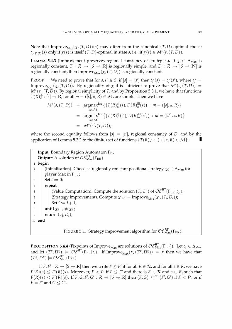
5.4. SOLVING OPTIMALITY EQUATIONS BY STRATEGY IMPROVEMENT 99
Note that ImproveMax(χ, (T, D))(s) may differ from the canonical (T, D)-optimal choiceχ(T,D)(s) only if χ(s) is itself (T, D)-optimal in state s, i.e., if χ(s) ∈ M∗(s, (T, D)).
LEMMA 5.4.3 (Improvement preserves regional constancy of strategies). If χ ∈ ∆Max isregionally constant, T : R → [S → R] is regionally simple, and D : R → [S → N] isregionally constant, then ImproveMax(χ, (T, D)) is regionally constant.
PROOF. We need to prove that for s, s′ ∈ S, if [s] = [s′] then χ′(s) = χ′(s′), where χ′ =ImproveMax(χ, (T, D)). By regionality of χ it is sufficient to prove that M∗(s, (T, D)) =M∗(s′, (T, D)). By regional simplicity of T, and by Proposition 5.3.1, we have that functionsT(R)⊕α : [s]→ R, for all m = ([s], α, R) ∈ M, are simple. Then we have
M∗(s, (T, D)) = argmaxlex
m∈M
(T(R)⊕α (s), D(R)α (s)
): m = ([s], α, R)
= argmaxlex
m∈M
(T(R)⊕α (s′), D(R)α (s′)
): m = ([s′], α, R)
= M∗(s′, (T, D)),
where the second equality follows from [s] = [s′], regional constancy of D, and by theapplication of Lemma 5.2.2 to the (finite) set of functions T(R)⊕α : ([s], α, R) ∈ M.
Input: Boundary Region Automaton ΓBR
Output: A solution of OERTMax(ΓBR)
begin1
(Initialisation). Choose a regionally constant positional strategy χ0 ∈ ∆Max for2
player Max in ΓBR;Set i := 0;3
repeat4
(Value Computation). Compute the solution (Ti, Di) of OERT(ΓBRχi);5
(Strategy Improvement). Compute χi+1 = ImproveMax(χi, (Ti, Di));6
Set i := i + 1;7
until χi+1 6= χi ;8
return (Ti, Di);9
end10
FIGURE 5.1. Strategy improvement algorithm for OERTMax(ΓBR).
PROPOSITION 5.4.4 (Fixpoints of ImproveMax are solutions of OERTMax(ΓBR)). Let χ ∈ ∆Max
and let (Tχ, Dχ) |= OERT(ΓBRχ). If ImproveMax(χ, (Tχ, Dχ)) = χ then we have that(Tχ, Dχ) |= OERT
Max(ΓBR).
If F, F′ : R → [S R] then we write F ≤ F′ if for all R ∈ R, and for all s ∈ R, we haveF(R)(s) ≤ F′(R)(s). Moreover, F < F′ if F ≤ F′ and there is R ∈ R and s ∈ R, such thatF(R)(s) < F′(R)(s). If F, G, F′, G′ : R → [S R] then (F, G) ≤lex (F′, G′) if F < F′, or ifF = F′ and G ≤ G′.
5.4. SOLVING OPTIMALITY EQUATIONS BY STRATEGY IMPROVEMENT 100
The following proposition characterises the solution of optimality equationsOERT(ΓBR)for a 0-player boundary region automaton ΓBR, as the lexicographically maximum solutionof the system of inequalities OERT
≤ (ΓBR).
PROPOSITION 5.4.5 (Solution of OERT(ΓBR) is the maximum solution of OERT≤ (ΓBR)). Let
T, T≤ : R → [S → R] and D, D≤ : R → [S → N] be such that (T, D) |= OERT(ΓBR) and(T≤, D≤) |= OERT
≤ (ΓBR). Then we have (T≤, D≤) ≤lex (T, D), and if (T≤, D≤) 6|= OERT(ΓBR)then the inequality is strict, i.e., we have (T≤, D≤) <lex (T, D).
PROOF. Our first goal is to establish that for every s ∈ S, we have (T≤(s), D≤(s)) ≤lex
(T(s), D(s)). We proceed by induction on D(s), i.e., on the length of the χ(T,D)-path in ΓBR
from [s] to a final region. The trivial base case is when [s] is a final region, because then(T(s), D(s)) = (0, 0) and (T≤(s), D≤(s)) ≤lex (0, 0). Let s ∈ S \ F be such that D(s) = n + 1.Then D(Succ(s, χ(T,D)(s))) = n and if χ(T,D)(s) = ([s], α, R′) then we have the following:(
T≤(s), D≤(s))≤lex
(T≤(R′)⊕α (s), D≤(R′)α (s)
)(5.4.1)
≤lex(T(R′)⊕α (s), D(R′)α (s)
)=
(T(s), D(s)
),
where the first inequality follows from (T≤, D≤) |= OERT≤ (ΓBR), the second inequality
follows from the induction hypothesis, and the last equality follows from (T, D) |=OERT(ΓBR) and χ(T,D)(s) = ([s], α, R′). This concludes the proof that (T≤, D≤) ≤lex (T, D).
We prove that if (T≤, D≤) 6|= OERT(ΓBR) then there is s ∈ S, such that (T≤(s), D≤(s)) <lex
(T(s), D(s)). Indeed, if (T≤, D≤) 6|= OERT(ΓBR) then either (T≤(s), D≤(s)) <lex (0, 0) forsome s ∈ F, or there is s ∈ S \ F, for which the inequality in (5.4.1) is strict and hence we get(T≤(s), D≤(s)) <lex (T(s), D(s)).
LEMMA 5.4.6 (Strict strategy improvement for player Max). Let χ, χ′ ∈ ∆Max, let (T, D) |=OERT
Min(ΓBRχ) and (T′, D′) |= OERTMin(ΓBRχ′), and let χ′ = ImproveMax(χ, (T, D)). Then
we have that (T, D) ≤lex (T′, D′) and if χ 6= χ′ then (T, D) <lex (T′, D′).
PROOF. First we argue that (T, D) |= OERT≤ (ΓBRχ′) which by Proposition 5.4.5 implies
that (T, D) ≤ (T′, D′). Indeed for every s ∈ S \ F, if χ(s) = ([s], α, R) and χ′(s) = ([s], α′, R′)then we have (
T(s), D(s))
=(T(R)⊕α (s), D(R)α (s)
)≤lex (
T(R′)⊕α′(s), D(R′)α′(s)),
where the equality follows from (T, D) |= OERTMin(ΓBRχ), and the inequality follows from
the definition of ImproveMax. Moreover, if χ 6= χ′ then there is s ∈ SMax \ F for which theabove inequality is strict. Then (T, D) 6|= OERT
Min(ΓBRχ′) because every vertex in ΓBRχ′
has a unique successor, and hence again by Proposition 5.4.5 we conclude that (T, D) <lex
(T′, D′).
The following theorem is an immediate corollary of Lemmas 5.4.2 and 5.4.3 (thealgorithm considers only regionally constant strategies), of Lemma 5.4.6 and finiteness of
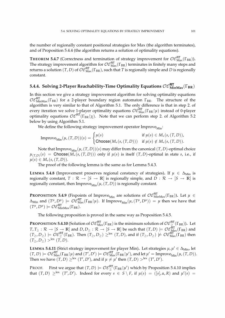
5.4. SOLVING OPTIMALITY EQUATIONS BY STRATEGY IMPROVEMENT 101
the number of regionally constant positional strategies for Max (the algorithm terminates),and of Proposition 5.4.4 (the algorithm returns a solution of optimality equations).
THEOREM 5.4.7 (Correctness and termination of strategy improvement for OERTMax(ΓBR)).
The strategy improvement algorithm for OERTMax(ΓBR) terminates in finitely many steps and
returns a solution (T, D) ofOERTMax(ΓBR), such that T is regionally simple and D is regionally
constant.
5.4.4. Solving 2-Player Reachability-Time Optimality Equations OERTMinMax(ΓBR)
In this section we give a strategy improvement algorithm for solving optimality equationsOERT
MinMax(ΓBR) for a 2-player boundary region automaton ΓBR. The structure of thealgorithm is very similar to that of Algorithm 5.1. The only difference is that in step 2. ofevery iteration we solve 1-player optimality equations OERT
Max(ΓBRµ) instead of 0-playeroptimality equations OERT(ΓBRχ). Note that we can perform step 2. of Algorithm 5.2below by using Algorithm 5.1.
We define the following strategy improvement operator ImproveMin:
ImproveMin(µ, (T, D))(s) =
µ(s) if µ(s) ∈ M∗(s, (T, D)),
Choose(M∗(s, (T, D))) if µ(s) 6∈ M∗(s, (T, D)).
Note that ImproveMin(µ, (T, D))(s) may differ from the canonical (T, D)-optimal choiceµ(T,D)(s) = Choose(M∗(s, (T, D))) only if µ(s) is itself (T, D)-optimal in state s, i.e., ifµ(s) ∈ M∗(s, (T, D)).
The proof of the following lemma is the same as for Lemma 5.4.3.
LEMMA 5.4.8 (Improvement preserves regional constancy of strategies). If µ ∈ ∆Min isregionally constant, T : R → [S → R] is regionally simple, and D : R → [S → R] isregionally constant, then ImproveMin(µ, (T, D)) is regionally constant.
PROPOSITION 5.4.9 (Fixpoints of ImproveMin are solutions of OERTMinMax(ΓBR)). Let µ ∈
∆Min and (Tµ, Dµ) |= OERTMax(ΓBRµ). If ImproveMin(µ, (Tµ, Dµ)) = µ then we have that
(Tµ, Dµ) |= OERTMinMax(ΓBR).
The following proposition is proved in the same way as Proposition 5.4.5.
PROPOSITION 5.4.10 (Solution ofOERTMax(ΓBR) is the minimum solution ofOERT
≥ (ΓBR)). LetT, T≥ : R → [S → R] and D, D≥ : R → [S → R] be such that (T, D) |= OERT
Max(ΓBR) and(T≥, D≥) |= OERT
≥ (ΓBR). Then (T≥, D≥) ≥lex (T, D), and if (T≥, D≥) 6|= OERTMax(ΓBR) then
(T≥, D≥) >lex (T, D).
LEMMA 5.4.11 (Strict strategy improvement for player Min). Let strategies µ, µ′ ∈ ∆Min, let(T, D) |= OERT
Max(ΓBRµ) and (T′, D′) |= OERTMax(ΓBRµ′), and let µ′ = ImproveMin(µ, (T, D)).
Then we have (T, D) ≥lex (T′, D′), and if µ 6= µ′ then (T, D) >lex (T′, D′).
PROOF. First we argue that (T, D) |= OERT≥ (ΓBRµ′) which by Proposition 5.4.10 implies
that (T, D) ≥lex (T′, D′). Indeed for every s ∈ S \ F, if µ(s) = ([s], α, R) and µ′(s) =
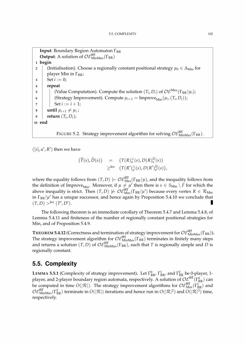
5.5. COMPLEXITY 102
Input: Boundary Region Automaton ΓBR
Output: A solution of OERTMinMax(ΓBR)
begin1
(Initialisation). Choose a regionally constant positional strategy µ0 ∈ ∆Min for2
player Min in ΓBR;Set i := 0;3
repeat4
(Value Computation). Compute the solution (Ti, Di) of OEMax(ΓBRµi);5
(Strategy Improvement). Compute µi+1 = ImproveMin(µi, (Ti, Di));6
Set i := i + 1;7
until µi+1 6= µi ;8
return (Ti, Di);9
end10
FIGURE 5.2. Strategy improvement algorithm for solving OERTMinMax(ΓBR).
([s], α′, R′) then we have(T(s), D(s)
)=
(T(R)⊕α (s), D(R)α (s)
)≥lex (
T(R′)⊕α′(s), D(R′)α′(s)),
where the equality follows from (T, D) |= OERTMax(ΓBRµ), and the inequality follows from
the definition of ImproveMin. Moreover, if µ 6= µ′ then there is s ∈ SMin \ F for which theabove inequality is strict. Then (T, D) 6|= OERT
Max(ΓBRµ′) because every vertex R ∈ RMinin ΓBRµ′ has a unique successor, and hence again by Proposition 5.4.10 we conclude that(T, D) >lex (T′, D′).
The following theorem is an immediate corollary of Theorem 5.4.7 and Lemma 5.4.8, ofLemma 5.4.11 and finiteness of the number of regionally constant positional strategies forMin, and of Proposition 5.4.9.
THEOREM 5.4.12 (Correctness and termination of strategy improvement forOERTMinMax(ΓBR)).
The strategy improvement algorithm for OERTMinMax(ΓBR) terminates in finitely many steps
and returns a solution (T, D) of OERTMinMax(ΓBR), such that T is regionally simple and D is
regionally constant.
5.5. ComplexityLEMMA 5.5.1 (Complexity of strategy improvement). Let Γ0
BR, Γ1BR, and Γ2
BR be 0-player, 1-player, and 2-player boundary region automata, respectively. A solution of OERT(Γ0
BR) canbe computed in time O(|R|). The strategy improvement algorithms for OERT
Max(Γ1BR) and
OERTMinMax(Γ2
BR) terminate in O(|R|) iterations and hence run in O(|R|2) and O(|R|3) time,respectively.
5.5. COMPLEXITY 103
PROOF. An O(|R|) algorithm to solve OERT(Γ0BR) is implicit in the proof of Lemma 5.4.2.
Let (T, D) |= OERTMax(Γ1
BR); and for all i ≥ 0, let χi ∈ ∆Max be the strategy in the i-thiteration of Algorithm 5.1, and let (Ti, Di) |= OERT(Γ1
BRχi). We claim that for every i ≥ 0, ifD(R) ≡ i then for all j ≥ i, we have (Tj(R), Dj(R)) = (T(R), D(R)). This can be establishedby a routine induction on the values of the regionally constant function D. Observe thatthe finite values of the function D are bounded by |R|, because in the proof of Lemma 5.4.2they are set to be the length of a simple path in a boundary region automaton. Algorithm 5.1must therefore terminate no later than after |R|+ 1 iterations, because for every i ≥ 0, inthe i-th iteration there must be R ∈ R whose value D(R) is set to i.
An analogous routine proof by induction on the value of D can be used to prove thatAlgorithm 5.2 terminates in O(|R|) iterations.
Since the number |R| of regions is at most exponential in the size of a timed automa-ton [AD94], we conclude that the strategy improvement algorithm solves reachability-timegames in exponential time.
COROLLARY 5.5.2. The problem of solving reachability-time games is in EXPTIME.
In order to prove EXPTIME-hardness of solving reachability-time games on timedautomata with two clocks, we reduce the EXPTIME-complete countdown games to reacha-bility games on timed automata.
THEOREM 5.5.3. The problem of solving reachability games is EXPTIME-complete on timedautomata with at least two clocks.
PROOF. In order to solve a reachability game on a timed automaton it is sufficient tosolve the reachability game on the finite region graph of the automaton. Observe that everyregion, and hence also every configuration of the game, can be written down in polynomialspace, and that every move of the game can be simulated in polynomial time. Therefore, thewinner in the game can be determined by a straightforward alternating PSPACE algorithm,and hence the problem is in EXPTIME because APSPACE = EXPTIME. In order to prove
n0 n12 3 2
A Countdown Game ((n0, B0) is the initial configuration)
(n0, 2) n0 (n0, 3) n1 (n1, 2)
*
c = 0, 2, c c = 0, 3, c c = 0, 2, c
c = 2, (n0, n0), c c = 3, (n0, n0), c c = 2, (n1, n1), c
b = B0, ∗, c b = B0, ∗, c
c = 3, (n0, n1), c
FIGURE 5.3. A Reduction from a Countdown Game to a Reachability Game.
5.5. COMPLEXITY 104
EXPTIME-hardness of solving reachability games on timed automata with two clocks, wereduce the EXPTIME-complete problem of solving countdown games [JLS07] to it.
Let G = (N, M, π, n0, B0) be a countdown game, where N is a finite set of nodes, M ⊆N × N is a set of moves, π : M → N+ assigns a positive integer number to every move,and (n0, B0) ∈ N ×N+ is the initial configuration. In every move of the game from aconfiguration (n, B) ∈ N ×N+, first player 1 chooses a number p ∈ N+, such that p ≤ Band π(n, n′) = p for some move (n, n′) ∈ M, and then player 2 chooses a move (n, n′′) ∈ M,such that π(n, n′′) = p; the new configuration is then (n′′, B− p). Player 1 wins a play ofthe game when a configuration (n, 0) is reached, and he loses (i.e., player 2 wins) when aconfiguration (n, B) is reached in which player 1 is stuck, i.e., for all moves (n, n′) ∈ M, wehave π(n, n′) > B.
We define the timed automaton TG = (L, C, S, A, E, δ, ξ, F) by setting C = b, c ; S =L× (JB0KR)2; A = ∗ ∪ P ∪M, where P = π(M), the image of the function π : M→N+;
L = ∗ ∪ N ∪(n, p) : there is (n, n′) ∈ M, s.t. π(n, n′) = p
;
E(a) =
(n, ν) : n ∈ N and ν(b) = B0 if a = ∗,(n, ν) : there is (n, n′) ∈ M, s.t. π(n, n′) = p and ν(c) = 0
if a = p ∈ P,(
(n, p), ν)
: π(n, n′) = p and ν(c) = p
if a = (n, n′) ∈ M,
δ(`, a) =
∗ if ` = n ∈ N and a = ∗,(n, p) if ` = n ∈ N and a = p ∈ P,
n′ if ` = (n, p) ∈ N × P and a = (n, n′) ∈ M;
ξ(a) = c , for every a ∈ A; and F = ∗ × VC. Note that the timed automaton TG hasonly two clocks and that the clock b is never reset.
Finally, we define the reachability game on timed game automaton ΓG = (TG, L1, L2)by setting L1 = N and L2 = L \ L1. It is routine to verify that player 1 has a winning strategyfrom state (n0, (0, 0)) ∈ S in the reachability game ΓG if and only if player 1 has a winningstrategy (from the initial configuration (n0, B0)) in the countdown game G. An example ofsuch reduction is shown in Figure 5.3.
The reachability games for timed automata can be easily reduced, in logarithmic space,to the reachability-time games so, by Theorem 5.5.3, reachability-time games are EXPTIME-hard. The following theorem follows from this observation and Corollary 5.5.2.
THEOREM 5.5.4 (Complexity of reachability-time games on timed automata). The problemof solving reachability-time games is EXPTIME-complete on timed automata with at leasttwo clocks.
6Average-Time Games
The truth is, you can’t goforever.
Tony Blair
An average-time game is played on the infinite graph of configurations of a finite timedautomaton. The two players, Min and Max, construct an infinite run of the automaton bytaking turns to perform a timed transition. Player Min wants to minimise the average timeper transition and player Max wants to maximise it. A solution of average-time games ispresented using a reduction to average-price games on finite graphs. A direct consequenceis an elementary proof of determinacy for average-time games. This complements ourresults for reachability-time games and partially solves a problem posed by Bouyer etal. [BBL04], to design an algorithm for solving average-price games on priced timedautomata. The exact computational complexity of solving average-time games is alsoestablished: the problem is EXPTIME-complete for timed automata with at least two clocks.
6.1. Introduction6.1.1. Definition
DEFINITION 6.1.1 (Average-Time Games). An average-time game on a timed automaton is atuple (Γ, ATMin, ATMax), where:
– Γ = (T , LMin, LMax) is a timed game automaton such that T = (L, C, S, A, E, δ, ξ, F)is a timed automaton, LMin is the set of locations controlled by player Min, and LMaxis the set of locations controlled by player Max;
– ATMin : Runs → R and ATMax : Runs → R are payoff functions, which for everyrun of the timed automaton return the amount the player Min loses and the playerMax wins, respectively. The functions ATMin and ATMax are defined as follows: fora run r = 〈s0, (t1, a1), s1, (t2, a2), . . .〉 ∈ Runs we have
ATMin(r) = lim supn→∞
1n
n
∑i=1
ti and ATMax(r) = lim infn→∞
1n
n
∑i=1
ti.
105
6.1. INTRODUCTION 106
We define QMin = (`, ν) ∈ Q : ` ∈ LMin, QMax = Q \ QMin, SMin = S ∩ QMin,SMax = S \ SMin,RMin = [s] : s ∈ QMin, andRMax = R \RMin.
The strategies of player Min and player Max are defined as usual (see Section 3.4.2). Wewrite ΣMin for the set of strategies for player Min, and we write ΣMax for the set of strategiesfor player Max. We write ΠMin and ΠMax for the sets of positional strategies for player Minand for player Max, respectively. Average-time payoff functions naturally give rise to thefunctions ATMin : S× ΣMin × ΣMax → R and ATMax : S× ΣMin × ΣMax → R in the followingway. For strategies µ ∈ ΣMin and χ ∈ ΣMax of respective players and a state s ∈ S we haveATMin(s, µ, χ) = ATMin(Run(s, µ, χ)) and ATMax(s, µ, χ) = ATMax(Run(s, µ, χ)).
6.1.2. Value of Average-Time Game
If player Min uses the strategy µ ∈ ΣMin and player Max uses the strategy χ ∈ ΣMax thenplayer Min loses the value ATMin(s, µ, χ) and player Max wins the value ATMax(s, µ, χ). Inan average-time game player Min is interested in minimising the value she loses and playerMax is interested in maximising the value he wins. We define the upper value Val(s) and thelower value Val(s) of the average-time game at the state s ∈ S by
Val(s) = infµ∈ΣMin
supχ∈ΣMax
ATMin(s, µ, χ), and Val(s) = supχ∈ΣMax
infµ∈ΣMin
ATMax(s, µ, χ).
By Proposition 1.2.4 the inequality Val(s) ≤ Val(s) always holds. An average-time game isdetermined if for every s ∈ S, the lower and upper values at s are equal to each other; thenwe say that the value Val(s) exists and Val(s) = Val(s) = Val(s).
We give an elementary proof for the determinacy of the average-time games withoutrecourse to general results like Martin’s determinacy theorem [Mar75, Mar98].
THEOREM 6.1.2 (Determinacy). Average-time games are determined.
For strategies µ ∈ ΣMin and χ ∈ ΣMax, we define
Valµ(s) = supχ∈ΣMax
ATMin(s, µ, χ), and Valχ(s) = infµ∈ΣMin
ATMax(s, µ, χ).
For an ε > 0, we say that a strategy µ ∈ ΣMin or χ ∈ ΣMax is ε-optimal if for every s ∈ S wehave that Valµ(s) ≤ Val(s) + ε or Valχ(s) ≥ Val(s)− ε, respectively. Note that if a game isdetermined then for every ε > 0, both players have ε-optimal strategies.
We say that a strategy χ ∈ ΣMax of player Max is a best response to a strategy µ ∈ ΣMin ofplayer Min if for all s ∈ S we have that ATMin(s, µ, χ) = supχ′∈ΣMax
ATMin(s, µ, χ′). Similarlywe say that a strategy µ ∈ ΣMin of player Min is a best response to a strategy χ ∈ ΣMax ofplayer Max if for all s ∈ S we have that ATMax(s, µ, χ) = infµ′∈ΣMin ATMax(s, µ′, χ).
In the next section we introduce some region-based abstractions of timed automata,including the closed region graph, and its subgraphs: the boundary region graph, and theregion graph. While the region graph is semantically equivalent to the corresponding timedautomaton, the boundary region graph has the property that for every starting state, thereachable state space is finite. In Section 6.4 we introduce average-time games on thesegraphs and show that if we have the solution of the average-time game for any of these
6.2. ABSTRACTIONS OF TIMED AUTOMATA 107
graphs, then we get the solution of the average-time game for the corresponding timedautomaton. The key Theorem 6.1.2 follows immediately from Theorem 6.4.2.
6.2. Abstractions of Timed AutomataThe corner-point abstraction, introduced by Bouyer et al. [BBL04], is a refinement of a regionautomaton which preserves some timing information. The corner-point abstraction TCP =(V, E) of a timed automaton T is a finite edge-labelled graph, where: V is a finite set ofvertices defined as
V = (s, R) ∈ Q×R : s = (`, ν) ∈ clos(R) and bνc = ν,and E is the labelled edge relation defined as
E = ((s, R), (t, R′′, a), (s′, R′)) ∈ V ×R⊕ ×R× A×V
: R −→∗ R′′ a−→ R′ and s′ = Succ(s, t, a) and s + t ∈ bd(R′′).From Proposition 3.7.13 we know that boundary region graphs are a generalisation of thecorner-point abstraction. We prove that the value of the average-time game on a timedautomaton is equal to the value of the average-time game on the corresponding boundaryregion graph for all starting states. In the process, we introduce two other relatedabstractions, which we call the closed region graph and the region graph. We collectively referto these three graphs as region graphs.
The analysis of average-time games on region graphs allows us to establish equivalenceof average-time games on the original timed automaton and the boundary region graph. Wealso show (Lemma 6.4.3) that the value of an average-time game is constant over a region.A side-effect of this result is that the corner-point abstractions can be used to solve average-time games on timed automata for arbitrary starting states.
6.2.1. Region Graphs
A configuration in region graphs is a is a pair (s, R), where s ∈ Q is a configuration of thetimed automaton and R ∈ R is a region; We write Ω for the set of configurations of theregion graphs. For a set X ⊆ Ω and a region R0 ∈ R, we define the set X restricted tothe region R0 as the set (s, R) ∈ X : R = R0, and we denote this set by X(R0). For aconfiguration q = (s, R) ∈ Ω we write write [q] for its region R.
DEFINITION 6.2.1 (Closed Region Graph). The closed region graph T = (S, E) of a timedautomaton T is a labelled transition system, where:
– S is the set of states defined as
S = (s, R) ∈ Ω : s ∈ clos(R) and
– E is the labelled transition relation defined as
E = ((s, R), (t, R′′, a), (s′, R′)) ∈ S× (R⊕ ×R× A)× S
: R −→∗ R′′ a−→ R′ and s′ = Succ(s, t, a) and s + t ∈ clos(R′′).
6.2. ABSTRACTIONS OF TIMED AUTOMATA 108
DEFINITION 6.2.2 (Boundary Region Graph). The boundary region graph T = (S, E) of atimed automaton T is a labelled transition system, where:
– S is the set of states defined as
S = (s, R) ∈ Ω : s ∈ clos(R) and
– E is the labelled transition relation defined as
E = ((s, R), (t, R′′, a), (s′, R′)) ∈ S× (R⊕ ×R× A)× S
: R −→∗ R′′ a−→ R′ and s′ = Succ(s, t, a) and s + t ∈ bd(R′′).
DEFINITION 6.2.3 (Region Graph). A region graph of a timed automaton T is a labelledtransition system T = (S, E), where:
– S is the set of states defined as
S = (s, R) ∈ Ω : s ∈ R and
– E is the labelled transition relation defined as
E = ((s, R), (t, R′′, a), (s′, R′)) ∈ S× (R⊕ ×R× A)× S
: R −→∗ R′′ a−→ R′ and s′ = Succ(s, t, a) and s + t ∈ R′′.
Notice that there are no significant differences between the definitions of the boundaryregion graph and the region graph presented above and those from Chapter 3. Wereproduce these definition to help the reader compare the three region graphs.
For configuration q = (s, R) ∈ Ω, real number t ∈ R⊕, region R′′ ∈ R, and actiona ∈ A, we write Succ(q, (t, R′′, a)) for the configuration
(Succ(s, t, a), R′
)where R′′ a−→ R′.
Recall from Definition 3.7.7 that A = A × JKKN × C is the finite set of boundary timedactions. For configuration q = (s, R) ∈ Ω, boundary timed action α = (b, c, a) ∈ A, andregion R′′ ∈ R we write Succ(q, (α, R′′)) for the configuration Succ(q, (t(s, α), R′′, a)).
6.2.2. Region Game Graphs
For Γ = (T , LMin, LMax) we define the sets ΩMin = (s, R) ∈ Ω : R ∈ RMin andΩMax = Ω \ΩMin. Similarly we define sets SMin, SMax, SMin, SMax, SMin, and SMax. The timedgame automaton Γ naturally gives rise to the closed region game graph Γ = (T , SMin, SMax),the boundary region game graph Γ = (T , SMin, SMax), and the region game graph Γ =(T , SMin, SMax). When it is clear from context, we use the terms region graphs and regiongame graphs interchangeably. Also, sometimes, we write T , T , T , and T for Γ, Γ, Γ, and Γ,respectively.
6.2.3. Runs of Region Graphs
An infinite run of the closed region graph T = (S, E) is an infinite sequence
〈q0, τ1, q1, τ1, . . .〉 ∈ S×((R⊕ ×R× A)× S
)ω,
6.2. ABSTRACTIONS OF TIMED AUTOMATA 109
such that for every positive integer i we have (qi−1, τi, qi) ∈ E. A finite run of the closedregion graph T is a finite sequence
〈q0, τ1, q1, τ1, . . . , qn〉 ∈ S×((R⊕ ×R× A)× S
)∗,such that for every positive integer i ≤ n we have (qi−1, τi, qi) ∈ E. Runs of the boundaryregion graph and the region graph are defined analogously.
For a graph G ∈ T , T , T we write RunsG for the set of its runs and RunsG(q) for theset of its runs from a state q ∈ Q. We write RunsGfin for the set of finite runs and RunsGfin(q)for the set of finite runs starting from a state q ∈ S.
6.2.4. Pre-Runs and Run Types Revisited
Pre-runs, first introduce in Subsection 4.3.3, generalise runs of T , T , and T , and allow usto compare the runs in T , T , and T in a uniform manner. On the other hand, the conceptof the type of a run allows us to compare pre-runs passing through the same sequence ofregions.
A pre-run is a sequence 〈(s0, R0), (t1, R′1, a1), (s1, R1), . . .〉 ∈ Ω× ((R⊕ ×R× A)×Ω)ω,
such that si+1 = Succ(si, (ti+1, ai+1)) and Ri −→∗ R′i+1ai+1−−→ Ri+1 for every i ∈ N. We
write PreRuns for the set of pre-runs and PreRuns(s, R) for the set of pre-runs starting from(s, R) ∈ Ω. The relation between various sets of runs is as follows: for all q ∈ Q we have
RunsT (q) ⊆ RunsT (q) ⊆ PreRuns(q) and
RunsT (q) ⊆ RunsT (q) ⊆ PreRuns(q).
Similarly, a finite pre-run is a finite sequence 〈(s0, R0), (t1, R′1, a1), (s1, R1), . . . , (sn, Rn)〉 ∈(Q×R)× ((R⊕ ×R× A)× (Q×R))∗ such that for every nonnegative integer i < n wehave that si+1 = Succ(si, (ti+1, ai+1)) and Ri −→∗ R′i
ai+1−−→ Ri. We write PreRunsfin for the setof finite pre-runs and PreRunsfin(s, R) for the set of finite pre-runs starting from (s, R) ∈ Ω.For a finite run r = 〈q0, (t1, R1, a1), q1, (t2, R2, a2), . . . , qn〉 ∈ PreRunsfin we define its totaltime as Time(r) = ∑n
i=1 ti, and we denote the last state of the run by Last(r) = qn.A run type is a sequence 〈R0, (R′1, a1), R1, (R′2, a2), . . .〉 ∈ R × ((R × A) × R)ω such
that for every i ∈ N we have that Ri −→∗ R′i+1a−→ Ri+1. We say that a pre-run
r = 〈(s0, R0), (t1, R′1, a1), (s1, R1), (t1, R′2, a2), . . .〉 is of the type 〈R0, (R′1, a1), R1, (R′2, a2), . . .〉.Also, we say that a run r = 〈s0, (t1, a1), s1, (t2, a2), . . .〉 of a timed automaton T is of the type〈R0, (R′1, a1), R1, (R′2, a2), . . .〉, where Ri = [si] and R′i+1 = [si + ti+1] for all i ∈ N. We alsodefine the type of a finite runs analogously.
For a (finite or infinite) run or pre-run r, we write JrKR for its type. We write Types forthe set of run types, and we write Types(R) for the set of run types starting from regionR ∈ R. Similarly we write Typesfin for the set of finite run types, and we write Typesfin(R)for the set of finite run types starting from region R ∈ R.
6.3. STRATEGIES IN REGION GRAPHS 110
6.3. Strategies in Region Graphs
In this section we define strategies of players in region graphs T , T , and T , and studysome of their properties. Strategies in T are called admissible strategies, while strategies in Tare called boundary strategies. We also introduce so-called type-preserving boundary strategieswhich are a key tool in proving the correctness of game reduction from timed automatato boundary region graph. In Section 6.4 we show that there are optimal type-preservingboundary strategies in T and T .
6.3.1. Pre-strategies and Strategies in T , T , TPre-strategies generalise the concept of strategies in region graphs, and allows us to discussthe strategies in T , T , and T in a uniform manner. We first define pre-strategies for playersin T , and then using that we define strategies for players in closed region graph, boundaryregion graph, and region graph.
DEFINITION 6.3.1 (Pre-strategies). A pre-strategy of player Min µ is a (partial) functionµ : PreRunsfin → R⊕ ×R× A, such that for a run r ∈ PreRunsfin, if Last(r) = (s, R) ∈ΩMin then µ(r) = (t, R′′, a) is defined, and it is such that R −→∗ R′′ a−→ R′ for some R′ ∈ R.Pre-strategies of player Max are defined analogously. We write Σpre
Min and ΣpreMax for the set of
pre-strategies of player Min and player Max, respectively.
We say that a strategy of player Min µ ∈ ΣpreMin is positional if for all runs r1, r2 ∈
PreRunsfin we have that Last(r1) = Last(r2) implies µ(r1) = µ(r2). Similarly we definepositional strategy of player Max.
We define the run starting from configuration q ∈ Ω where player Min and player Maxuse the strategies µ ∈ Σpre
Min and χ ∈ ΣpreMax, respectively, in a straightforward manner and we
write Run(q, µ, χ) for this run. For every positive integer n we write Runn(q, µ, χ) for theprefix of the run Run(q, µ, χ) of length n.
Now we are in a position to introduce strategies in closed region graph, region graph,and boundary region graph.
DEFINITION 6.3.2 (Strategies in Closed Region Graph). A pre-strategy of player Minµ ∈ Σpre
Min is a strategy in a closed region graph T = (S, E) if for every run r ∈ PreRunsfinsuch that µ(r) = (t, R′, a), we have that (s + t) ∈ clos(R′) where (s, R) = Last(r). Strategiesof player Max in a closed region graph are defined analogously. We write ΣMin and ΣMax forthe set of strategies of player Min and player Max, respectively.
DEFINITION 6.3.3 (Strategies in Region Graphs). A pre-strategy of player Min µ ∈ ΣpreMin is a
strategy in a region graph T = (S, E) if for every run r ∈ RunsTfin such that µ(r) = (t, R′′, a),we have that (s + t) ∈ R′′ where (s, R) = Last(r). Strategies of player Max in a regiongraph are defined analogously. We call such strategies admissible strategies. We write ΣMin
and ΣMax for the set of admissible strategies of player Min and player Max, respectively.
DEFINITION 6.3.4 (Strategies in Boundary Region Graph). A pre-strategy of player Minµ ∈ Σpre
Min is a strategy in a boundary region graph T = (S, E) if for every run r ∈ PreRunsfin
6.3. STRATEGIES IN REGION GRAPHS 111
such that µ(r) = (t, R′, a), we have that
t = inft : s + t ∈ clos(R′), (6.3.1)
where (s, R) = Last(r).A pre-strategy of player Max χ ∈ Σpre
Max is a strategy in a boundary region graph T if forevery run r ∈ PreRunsfin such that µ(r) = (t, R′, a), we have that
t = supt : s + t ∈ clos(R′), (6.3.2)
where (s, R) = Last(r). We call such strategies boundary strategies. We write ΣMin and ΣMaxfor the set of boundary strategies of player Min and player Max, respectively.
For notational convenience and w.l.o.g., in the definition of boundary strategies, we donot consider those timed moves of player Min (Max) which suggest waiting till the farther(nearer) boundary of a thick region.
FACT 6.3.5. For every state s ∈ S of timed automata T and every strategy µ ∈ ΣpreMin and
χ ∈ ΣpreMax of respective players, we have that :
– Run((s, [s]), µ, χ) ∈ RunsT (s, [s]) if µ ∈ ΣMin and χ ∈ ΣMax;– Run((s, [s]), µ, χ) ∈ RunsT (s, [s]) if µ ∈ ΣMin and χ ∈ ΣMax;– Run((s, [s]), µ, χ) ∈ RunsT (s, [s]) if µ ∈ ΣMin and χ ∈ ΣMax.
Boundary Strategies and Boundary Timed Actions. Timed actions suggested by a bound-ary strategies are precisely boundary timed actions as defined in Definition 3.7.7. Thefollowing proposition formalises this notion.
PROPOSITION 6.3.6. For every boundary strategy σ ∈ ΣMin(ΣMax) of player Min (Max) andfor every run r ∈ PreRunsfin, if σ(r) = (t, R′, a) then there exists a boundary timed actionα = (b, c, a) ∈ A such that t(s, α) = t, where (s, R) = Last(r).
PROOF. Let run r ∈ PreRunsfin be such that Last(r) = (s, R). Let σ ∈ ΣMin be a boundarystrategy of player Min such that σ(r) = (t, R′, a). From the definition of the boundarystrategies, we have that t = inft : s + t ∈ clos(R′). To prove the proposition, all we needto show is that there exists an integer b ∈ Z and a clock c ∈ C, such that b− s(c) = t.
If R′ ∈ RThin then there exists a clock c′ ∈ C such that for all states s′ ∈ clos(R′) wehave that *s′(c′)+ = 0. In this case the clock c = c′ and the integer b = (s + t)(c).
If R ∈ RThick and let R′ ←−+1 R be the thin region immediately before R. Let clockc′ ∈ C be such that for all states s′ ∈ clos(R′) we have that *s′(c′)+ = 0. Again, in this casethe desired clock c = c′ and the integer b = (s + t)(c).
The case, where σ is a strategy of Max is similar, and hence omitted.
Sometimes, in our proofs we need to use boundary timed action suggested by aboundary strategy. For this purpose we define the notation σbta(r) that gives the boundarytimed action and region pair that corresponds to σ(r). The definition of this function isformalised in the following definition.
6.3. STRATEGIES IN REGION GRAPHS 112
DEFINITION 6.3.7. For a boundary strategy σ ∈ ΣMax(ΣMax) of player Min (Max), we definethe function σbta : PreRunsfin → (A×R) as follows: if for a run r ∈ PreRunsfin we haveσ(r) = (t, R′, a), then σbta(r) = ((b, c, a), R′) such that b− s(c) = t, where (s, R) = Last(r).
6.3.2. Type-Preserving Boundary Strategies
We now introduce an important class of boundary strategies called type-preserving boundarystrategies. Broadly speaking, these strategies suggest to players a unique boundary timedaction and region pair for all the finite runs of the same type.
DEFINITION 6.3.8 (Type-Preserving Boundary Strategies). A boundary strategy σ ∈ ΣMinof player Min is type-preserving if Jr1KR = Jr2KR implies σbta(r1) = σbta(r2) for all r1, r2 ∈PreRunsfin. Type-preserving boundary strategies of player Max are defined analogously.We write ΞMin and ΞMax for the sets of type-preserving boundary strategies of players Minand Max, respectively.
The rationale behind the name type-preserving is that if µ ∈ ΞMin and χ ∈ ΞMax, then forevery R ∈ R and for q, q′ ∈ Ω(R), the run types of the resulting runs from q and q′ are thesame, i.e., JRun(q, µ, χ)KR = JRun(q′, µ, χ)KR.
6.3.2.1. Simple Functions Revisited
Let us redefine simple functions in the context of region graphs. Let X ⊆ Ω. A functionF : X → R is a simple function if either: there is e ∈ Z, such that for every q = (s, R) ∈ X, wehave F(q) = e; or there are e ∈ Z and c ∈ C, such that for every q = (s, R) ∈ X, we haveF(q) = e− s(c). We say that a function F : X → R is regionally simple or regionally constant,respectively, if for every region R ∈ R, the function F, over domain X(R), is simple orconstant, respectively.
For regions R, R′, R′′ ∈ R and boundary timed action α = (b, c, a) ∈ A, we write
R R′′−→α R′ if one of the following holds:
– R −→b,c R′′ a−→ R′, or– there is region R′′′ ∈ RThin such that R −→b,c R′′′ −→+1 R′′ a−→ R′, or– there is a region R′′′ ∈ RThin such that R −→b,c R′′′ ←−+1 R′′ a−→ R′.
The proof of the following proposition is along the lines of the proof of Proposition 5.3.1.
PROPOSITION 6.3.9. Let α ∈ A and regions R, R′, R′′ ∈ R be such that R R′′−→α R′. Ifa function F : Ω(R′) → R is simple then the function F⊕(α,R′′) : Ω(R) → R, defined as(s, R) 7→ t(s, α) + F(Succ(q, (α, R′′))), is simple.
The proof of the following proposition is analogous to the proof of Proposition 5.3.2.
PROPOSITION 6.3.10. Let a ∈ A and regions R, R′, R′′ ∈ R be such that R −→∗ R′′ a−→ R′.If a function F : Ω(R′) → R is simple then for every q = (s, R) ∈ Ω(R), the functionF⊕(q,R′′,a) : I → R, defined as t 7→ t + F(Succ(q, (t, R′′, a))), is continuous and nondecreasing,where I = t ∈ R⊕ : (s + t) ∈ clos(R′′).
6.3. STRATEGIES IN REGION GRAPHS 113
6.3.2.2. Properties of Type-preserving Boundary Strategies
The next two proposition state that if both players play with type-preserving boundarystrategies then for every n ∈ N the total time spent in n transitions is regionallysimple (Proposition 6.3.11), and the average time of the infinite run is regionally constant(Proposition 6.3.12).
PROPOSITION 6.3.11 (Type-preserving strategy pairs yield regionally simple time for finiteruns). If µ ∈ ΞMin, χ ∈ ΞMax, and n ∈ N, then Time(Runn(·, µ, χ)) : Q → R⊕ is regionallysimple.
PROOF. Let µ ∈ ΞMin and χ ∈ ΞMax. We prove this lemma by induction on the value of n.The base case for n = 0 is trivial. Assume that for every µ ∈ ΞMin and χ ∈ ΞMax the functionTime(Runk(·, µ, χ)) : Q → R⊕ is regionally simple. To prove this proposition we now needto show that for µ ∈ ΞMin and χ ∈ ΞMax the function Time(Runk+1(·, µ, χ)) is regionallysimple.
Let the strategies µ′ ∈ ΞMin and χ′ ∈ ΞMax be such that for every q ∈ Q the runRunk(Succ(q, µ, χ), µ′, χ′) be the length k suffix of the run Runk+1(q, µ, χ). From inductivehypothesis we have that Runk(·, µ′, χ′) is regionally simple. Assume that R ∈ RMin andlet µbta(〈q〉) = (α, R′′) for every q ∈ Q(R). The treatment for the case where R ∈ RMax issimilar. Now for every q = (s, R) ∈ Q(R) we have that Time(Runk+1(q, µ, χ)) = t(s, α) +Runk(Succ(q, (α, R′′)), µ′, χ′), which from Proposition 6.3.9 is a simple function.
PROPOSITION 6.3.12 (Type-preserving strategy pairs yield regionally constant averagetime). If µ ∈ ΞMin and χ ∈ ΞMax then ATMin(·, µ, χ) : Q → R⊕ and ATMax(·, µ, χ) : Q → R⊕are regionally constant.
PROOF. Let µ ∈ ΞMin, χ ∈ ΞMax and q = (s, R), q′ = (s′, R) ∈ Q(R). We have
ATMin(q, µ, χ)− ATMin(q′, µ, χ)
= lim infn→∞
(1/n) · Time(Runn(q, µ, χ))− lim infn→∞
(1/n) · Time(Runn(q′, µ, χ))
= lim infn→∞
(1/n) ·(b− s(c)− b + s′(c)
)= lim inf
n→∞(1/n) ·
(s′(c)− s(c)
)= 0.
The first equality is by definition, the second follows from Proposition 6.3.11, and the lasttwo equalities are trivial. Similarly we show that ATMax(q, µ, χ) = ATMax(q′, µ, χ).
6.3.2.3. Type-preserving Boundary Strategy that Agrees with a Boundary Strategy
Given an arbitrary boundary strategy σ and a configuration q ∈ Q, sometimes we areinterested in a type-preserving boundary strategy that agrees with σ for all the runs startingfrom q. We denote such a strategy by σ↓q. The following definition formalises such strategy.
DEFINITION 6.3.13. For a boundary strategy µ ∈ ΣMin of player Min and q ∈ Q wedefine µ↓q ∈ ΞMin to be a type-preserving boundary strategy which satisfy the followingconditions:
6.3. STRATEGIES IN REGION GRAPHS 114
(1) µ↓qbta(r) = µbta(r) for every r ∈ PreRunsfin(q), and
(2) JrKR = Jr′KR implies µ↓qbta(r) = µ
↓qbta(r′) for all runs r, r′ ∈ PreRunsfin.
For χ ∈ ΣMax and q ∈ Q we define χ↓q ∈ ΞMax analogously.
Given an arbitrary strategy µ ∈ ΣMin of player Min, a type-preserving boundarystrategy χ ∈ ΞMax of player Max, and a configuration q ∈ Q sometimes we require tospecify a type-preserving strategy µ(q,χ) ∈ ΞMin which has the property that types of runsRun(q, µ, χ) and Run(q, µ(q,χ), χ) are the same. We then argue that from configuration q ∈ Qif player Max plays according to χ ∈ ΞMax then player Min can achieve better average-timeif she plays according to µ(q,χ) (see Proposition 6.3.15 and Corollary 6.3.16). The motivationfor the definition of χ(q,µ) is similar.
DEFINITION 6.3.14. For an arbitrary strategy µ ∈ ΣMin of player Min, a type-preservingboundary strategy χ ∈ ΞMax of player Max, and a configuration q = (s, R) ∈ Q, wedefine µ(q,χ) ∈ ΞMin to be a type-preserving boundary strategy which satisfy the followingconditions:
(1) JRun(q, µ(q,χ), χ)KR = JRun(q, µ, χ)KR, and(2) JrKR = Jr′KR implies µ
(q,χ)bta (r) = µ
(q,χ)bta (r′) for all runs r, r′ ∈ PreRunsfin.
For χ ∈ ΣMax, µ ∈ ΞMin, and q ∈ Q the strategy χ(q,µ) ∈ ΞMax is defined analogously.
The following proposition and its corollary shows that starting from a configuration qplayer Min (Max) prefers µ(q,χ) (χ(q,µ)) to µ (χ) against a type-preserving strategy χ ∈ ΞMax(µ ∈ ΞMin) of its opponent.
PROPOSITION 6.3.15. For every χ ∈ ΞMax, µ ∈ ΣMin and q ∈ Q we have that
Time(Runn(q, µ, χ)) ≥ Time(Runn(q, µ(q,χ), χ)),
for every n ∈N. Similarly, for every µ ∈ ΞMin, χ ∈ ΣMax and q ∈ Q we have that
Time(Runn(q, µ, χ)) ≤ Time(Runn(q, µ, χ(q,µ))),
for every n ∈N.
PROOF. The proof is by induction on n. The base case, when n = 0, is trivial. In the restof the proof we show that for χ ∈ ΞMax, µ ∈ ΣMin, and a configuration q = (s, R) ∈ Q, wehave that Time(Runk+1(q, µ, χ)) ≥ Time(Runk+1(q, µ(q,χ), χ)) assuming that the propositionholds for n = k. The proof for the case where q ∈ QMax is trivial. In the rest of the proof weassume that q ∈ QMin.
Let us fix χ ∈ ΞMax and µ ∈ ΣMin. Let the runs Runk+1(q, µ, χ) and Runk+1(q, µ(q,χ), χ)be 〈q0, τ1, q1, . . . , qk+1〉 and 〈q′0, τ′1, q′1, . . . , q′k+1〉, respectively, where q0 = q′0 = q. Notice thatby definition the run types of both runs are the same. Hence for every index i ≤ k + 1 wehave qi = (si, Ri) and q′i = (s′i, Ri), and for every index i ≤ k + 1 we have τi = (ti, R′i, ai) andτ′i = (t′i, R′i, ai).
Let X ∈ ΞMax and M ∈ ΣMin be such that the run Runk(q1, M, X) be length k suffix ofthe run Runk+1(q, µ, χ). Notice that we assume that X is type-preserving. It is easy to see
6.3. STRATEGIES IN REGION GRAPHS 115
thatTime(Runk+1(q, µ, χ)) = t1 + Time(Runk(q1, M, X)).
From inductive hypothesis, we get that
Time(Runk+1(q, µ, χ)) ≥ t1 + Time(Runk(q1, M(q1,X), X)). (6.3.3)
Since the strategies M(q1,X) ∈ ΞMin and X ∈ ΞMax are type-preserving, from Proposi-tion 6.3.11 we get that Time(Runk(·, M(q1,X), X)) is regionally simple. Let us denote therestriction of this function on domain Q(R1) by F : Q(R1) → R. Let us define the partialfunction F⊕(q,R′1,a) : R⊕ R as t 7→ t + F (Succ(q, (t, R′′, a))), for all t ∈ R⊕, such that(s + t) ∈ clos(R′1). The following inequality follows from (6.3.3):
Time(Runk+1(q, µ, χ)) ≥ t1 +F (q1) ≥ inft
F⊕(q,R′1,a)(t) : s + t ∈ clos(R′1)
.
Since µ(q,χ) is a type-preserving boundary strategy of player Min, from equation (6.3.1), weknow that t′1 = inft : s + t ∈ clos(R′1). Moreover from Proposition 6.3.10 we have thatF⊕(q,R′1,a) is continuous and nondecreasing on the domain t ∈ R⊕ : (s + t) ∈ clos(R′′).Hence F⊕(q,R′1,a)(t′1) = inft
F⊕(q,R′1,a)(t) : s + t ∈ clos(R′1)
. Combining these facts, we get
the following inequalities:
Time(Runk+1(q, µ, χ)) ≥ F⊕(q,R′1,a)(t′1) = t′1 + Time(Runk(q′1, M(q1,X), X))
Since the run Runk(q′1, M(q1,X), X) is length k suffix of the run Runk+1(q, µ(q,χ), χ), weget the desired inequality.
An easy corollary of this proposition is as follows:
COROLLARY 6.3.16. For every χ ∈ ΞMax, µ ∈ ΣMin and for all configurations q ∈ Q we havethat
ATMin(q, µ, χ)) ≥ ATMin(q, µ(q,χ), χ)).
Similarly for every µ ∈ ΞMin, χ ∈ ΣMax and for all configurations q ∈ Q we have that
ATMax(q, µ, χ)) ≤ ATMax(q, µ, χ(q,µ))).
6.3.2.4. Admissible Strategies ε-Close to a Type-Preserving Boundary Strategy
DEFINITION 6.3.17 (Set of Admissible Strategies ε-close to a Type-Preserving BoundaryStrategy). For µ ∈ ΞMin and a real number ε > 0, we define the set of admissible strategyΣ(µ,ε)
Min ⊆ ΣMin as follows. For every µε ∈ Σ(µ,ε)Min we have that for all runs r ∈ PreRunsfin if
µbta(r) = ((b, c, a), R′) then µε(r) = (t, R′, a) is such that
s + t ∈ R′ and t ≤ b− s(c) + ε,
where (s, R) = Last(r). Notice that (see Equation 6.3.1) such a value of t always exists.Similarly for χ ∈ ΞMax and a real number ε > 0 we define the set Σ(χ,ε)
Max ⊆ ΣMax as follows.
6.3. STRATEGIES IN REGION GRAPHS 116
For every χε ∈ Σ(χ,ε)Max we have that for all runs r ∈ PreRunsfin if χbta(r) = ((b, c, a), R′) then
χε(r) = (t, R′, a) is such that
s + t ∈ R′ and t ≥ b− s(c)− ε,
where (s, R) = Last(r).
Given an arbitrary strategy µ ∈ ΣMin of player Min, a positive real ε > 0, a type-preserving boundary strategy χ ∈ ΞMax of player Max, an ε-close strategy χε ∈ Σ(χ,ε)
Max ,and a configuration q ∈ Q sometimes we require to specify a type-preserving strategyµ(q,χε) ∈ ΞMin which has the property that types of runs Run(q, µ, χε) and Run(q, µ(q,χε), χε)are the same.
DEFINITION 6.3.18. For an arbitrary strategy µ ∈ ΣMin of player Min, a positive real ε > 0,a type-preserving boundary strategy χ ∈ ΞMax of player Max, an ε-close strategy χε ∈ Σ(χ,ε)
Max ,and a configuration q = (s, R) ∈ Q, we define µ(q,χε) ∈ ΞMin to be a type-preservingboundary strategy which satisfy the following conditions:
(1) JRun(q, µ(q,χε), χε)KR = JRun(q, µ, χε)KR, and(2) JrKR = Jr′KR implies µ
(q,χε)bta (r) = µ
(q,χε)bta (r′) for all runs r, r′ ∈ PreRunsfin.
Combining it with Definition 6.3.17 we get that JRun(q, µ(q,χε), χ)KR = JRun(q, µ, χε)KR.For χ ∈ ΣMax, χε ∈ Σ(χ,ε)
Max , µ ∈ ΞMin, and q ∈ Q the strategy χ(q,µε) ∈ ΞMax is definedanalogously.
We need the following property of µ(q,χε) and χ(q,µε) strategies.
PROPOSITION 6.3.19. For every arbitrary strategy µ ∈ ΣMin, positive real ε > 0, type-preserving boundary strategy χ ∈ ΞMax of player Max, ε-close strategy χε ∈ Σ(χ,ε)
Max of playerMax, and q ∈ Q we have
Time(Runn(q, µ, χε)) ≥ Time(Runn(q, µ(q,χε), χ))− n · ε,
for every n ∈ N. Similarly for every arbitrary strategy χ ∈ ΣMax, positive real ε > 0, type-preserving boundary strategy µ ∈ ΞMin of player Max, ε-close strategy µε ∈ Σ(µ,ε)
Min of playerMin, and q ∈ Q we have
Time(Runn(q, µε, χ)) ≤ Time(Runn(q, µε, χ(q,µε))) + n · ε,
for every n ∈N.
PROOF. The proof is by induction on n. The base case, when n = 0, is trivial. In the restof the proof we show that for χ ∈ ΞMax, µ ∈ ΣMin, ε > 0, χε ∈ Σ(χ,ε)
Max , and a configurationq = (s, R) ∈ Q, we have that Time(Runk+1(q, µ, χε)) ≥ Time(Runk+1(q, µ(q,χε), χ)) − k · ε,assuming that the proposition holds for n = k.
Let us fix χ ∈ ΞMax, µ ∈ ΣMin, ε > 0, and χε ∈ Σ(χ,ε)Max . Let the run Runk+1(q, µ, χε)
and the run Runk+1(q, µ(q,χε), χ) be 〈q0, τ1, q1, . . . , qk+1〉 and 〈q′0, τ′1, q′1, . . . , q′k+1〉, respectively,
6.3. STRATEGIES IN REGION GRAPHS 117
where q0 = q′0 = q. Notice that by definition the run types of both runs are the same. Hencefor every index i ≤ k + 1 we have qi = (si, Ri) and q′i = (s′i, Ri), and for every index i ≤ k + 1we have τi = (ti, R′i, ai) and τ′i = (t′i, R′i, ai).
Let X ∈ ΞMax and M ∈ ΣMin be such that the run Runk(q1, M, Xε) be length k suffix ofthe run Runk+1(q, µ, χε). Notice that we assume that X is type-preserving. It is easy to seethat
Time(Runk+1(q, µ, χε)) = t1 + Time(Runk(q1, M, Xε)).
From inductive hypothesis, we get that
Time(Runk+1(q, µ, χε)) ≥ t1 + Time(Runk(q1, M(q1,Xε), X))− k · ε. (6.3.4)
Since the strategies M(q1,Xε) ∈ ΞMin and X ∈ ΞMax are type-preserving boundary strategies,from Proposition 6.3.11 we get that Time(Runk(·, M(q1,Xε), X)) is regionally simple. Let usdenote the restriction of this function on domain Q(R1) by F : Q(R1) → R. Let us definethe partial function F⊕(q,R′1,a) : R⊕ R as t 7→ t +F (Succ(q, (t, R′′, a))), for all t ∈ R⊕, suchthat (s + t) ∈ clos(R′1). The following inequality follows from (6.3.4):
Time(Runk+1(q, µ, χε)) ≥ t1 +F (q1)− k · ε ≥ inft
F⊕(q,R′1,a)(t) : s + t ∈ clos(R′1)
− k · ε.
We need to consider two cases: q ∈ QMin and q ∈ QMax.– Assume that q ∈ QMin. Since µ(q,χε) is a type-preserving boundary strategy of
player Min, from equation (6.3.1), we know that t′1 = inft : s + t ∈ clos(R′1).Moreover from Proposition 6.3.10 we have that F⊕(q,R′1,a) is continuous and non-
decreasing on the domain t ∈ R⊕ : (s + t) ∈ clos(R′′). Hence F⊕(q,R′1,a)(t′1) =
inftF⊕(q,R′1,a)(t) : s + t ∈ clos(R′1)
. Combining these facts, we get the following
inequalities:
Time(Runk+1(q, µ, χε)) ≥ t′1 + Time(Runk(q′1, M(q1,Xε), X))− k · ε.
Since the run Runk(q′1, M(q1,Xε), X) is length k suffix of the run Runk+1(q, µ(q,χε), χ),we get the following inequality:
Time(Runk+1(q, µ, χε)) ≥ Time(Runk+1(q, µ(q1,χε), χ))− k · ε≥ Time(Runk+1(q, µ(q1,χε), χ))− (k + 1) · ε,
as required.– Assume that q ∈ QMax. So far we have shown that
Time(Runk+1(q, µ, χε)) ≥ t1 +F (q1)− k · ε. (6.3.5)
Since F is a simple function let F ((s1, R1)) = b− s1(c) for all (s1, R1) ∈ Q(R1). Forall t ∈ R⊕ such that s + t ∈ R′1 we have the following observation.
t +F ((Succ(s, (t, a1))) =
t + b if c ∈ ξ(a1)b− s(c) otherwise.
(6.3.6)
6.4. AVERAGE-TIME GAMES ON REGION GRAPHS 118
By Definition 6.3.17 we know that t1 ≥ t′1 − ε. Combining this with (6.3.6) we getthat
t1 +F (q1) ≥ t′1 +F (q′1)− ε.
We can then rewrite (6.3.5) as the following:
Time(Runk+1(q, µ, χε)) ≥ t′1 +F (q′1)− (k + 1) · ε.
The term F (q′1) represents the sum of the times of the run Runk(q′1, M(q1,Xε), X).Since the run Runk(q′1, M(q1,Xε), X) is length k suffix of the run Runk+1(q, µ(q,χε), χ),we get the inequality
Time(Runk+1(q, µ, χε)) ≥ Time(Runk+1(q, µ(q,χε), χ))− (k + 1) · ε,
as required.
The following result is an easy corollary of Proposition 6.3.19.
COROLLARY 6.3.20. For every χ ∈ ΞMax, µ ∈ ΣMin, ε > 0, χε ∈ Σ(χ,ε)Max , and q ∈ Q we have
thatATMax(q, µ, χε)) ≥ ATMax(q, µ(q,χε), χ))− ε.
Similarly for every µ ∈ ΞMin, χ ∈ ΣMax, ε > 0, µε ∈ Σ(µ,ε)Min , and q ∈ Q we have that
ATMin(q, µε, χ) ≤ ATMin(q, µ, χ(q,µε)) + ε.
To summarise the relations between various strategies, note that the following inclu-sions hold:
ΞMin ⊆ ΣMin ⊆ ΣMin ⊆ ΣpreMin and ΣMin ⊆ ΣMin ⊆ Σpre
Min, and
ΞMax ⊆ ΣMax ⊆ ΣMax ⊆ ΣpreMax and ΣMax ⊆ ΣMax ⊆ Σpre
Max.
6.4. Average-Time Games on Region GraphsWe define the functions ATMin : Ω×Σpre
Min×ΣpreMax → R⊕ and ATMax : Ω×Σpre
Min×ΣpreMax → R⊕
in the following manner:
ATMin(q, µ, χ) = lim supn→∞
1n· Time(Runn(q, µ, χ)), and
ATMax(q, µ, χ) = lim infn→∞
1n· Time(Runn(q, µ, χ)),
where µ ∈ ΣpreMin, χ ∈ Σpre
Max and q ∈ Ω. For average-time games on a graph G ∈ T , T , T we define the lower-value ValG(q), the upper-value Val
G(q) and the value ValG(q) of a
configuration q ∈ Q in a straightforward manner (for details, see Subsection 6.1.2).
6.4. AVERAGE-TIME GAMES ON REGION GRAPHS 119
From Proposition 3.7.5 it is clear that the difference between an average-time game ona timed automaton and the average-time game on corresponding region graph is purelysyntactical. Hence if the average-time game on region graph T is determined then average-time game on timed automaton T is determined as well.
PROPOSITION 6.4.1. An average-time game on timed automaton T is determined, if thecorresponding average-time game on region graph T is determined. Moreover for all s ∈ Swe have that Val(s) = ValT (s, [s]).
The following is the main result of this section.
THEOREM 6.4.2. Let T be a timed automaton. Average-time games on the timed automa-ton T , the closed region graph T , the region graph T , and the boundary region graph T aredetermined. Moreover for every s ∈ S in a timed automaton T , we have:
ValT (s) = ValT (s, [s]) = ValT (s, [s]) = ValT (s, [s]).
This theorem follows from Theorem 6.4.4, Theorem 6.4.8, Theorem 6.4.10, and Proposi-tion 6.4.1.
Moreover Theorem 6.4.2 and Proposition 6.3.12 let us conclude the following lemmaabout the value of average-time games on timed automata.
LEMMA 6.4.3. The value of every average-time game is regionally constant.
An interesting implication of Lemma 6.4.3 is that corner-point abstraction is sufficientto solve average-time games with an arbitrary initial state.
6.4.1. Determinacy of Average-Time Games on the Boundary Region Graph
Positional determinacy of average-time games on the boundary region graph is immediatefrom Proposition 3.7.10 and Theorem 2.3.3.
THEOREM 6.4.4. The average-time game on T is determined, and there are optimalpositional strategies in T , i.e., for every q ∈ Q, we have:
ValT (q) = infµ∈ΠMin
supχ∈ΣMax
ATMin(q, µ, χ) = supχ∈ΠMax
infµ∈ΣMin
ATMax(q, µ, χ).
LEMMA 6.4.5. In T , if µ ∈ ΣMin and χ ∈ ΣMax are mutual best responses from q ∈ Q, thenµ↓q ∈ ΞMin and χ↓q ∈ ΞMax are mutual best responses from every q′ ∈ Q([q]).
PROOF. We argue that χ↓q is a best response to µ↓q from q′ ∈ Q([q]) in T ; the other case isanalogous. For all X ∈ ΣMax, we have the following:
ATMin(q′, µ↓q, χ↓q) = ATMin(q, µ↓q, χ↓q) ≥ ATMin(q, µ↓q, X↓q′) =
ATMin(q′, µ↓q, X↓q′) = ATMin(q′, µ↓q, X).
6.4. AVERAGE-TIME GAMES ON REGION GRAPHS 120
The first equality follows from Proposition 6.3.12; the inequality follows because χ is a bestresponse to µ from q; the second equality follows from Proposition 6.3.12 again; and the lastequality is straightforward.
THEOREM 6.4.6. There are optimal type-preserving boundary strategies in T , i.e., for everyq ∈ Q, we have:
ValT (q) = infµ∈ΞMin
supχ∈ΣMax
ATMin(q, µ, χ) = supχ∈ΞMax
infµ∈ΣMin
ATMax(q, µ, χ).
PROOF. Let µ∗ ∈ ΞMin and χ∗ ∈ ΞMax be mutual best responses in T ; existence of suchstrategies follows from Lemma 6.4.5. Moreover, we can assume that the strategies µ∗ andχ∗ have finite memory; this can be achieved by taking positional strategies µ ∈ ΣMin andχ ∈ ΣMax in Lemma 6.4.5. We then have the following:
infµ∈ΞMin
supχ∈ΣMax
ATMin(q, µ, χ) ≤ supχ∈ΣMax
ATMin(q, µ∗, χ) = ATMin(q, µ∗, χ∗) =
ATMax(q, µ∗, χ∗) = infµ∈ΣMin
ATMax(q, µ, χ∗) ≤ supχ∈ΞMax
infµ∈ΣMin
ATMax(q, µ, χ).
The first and last inequalities are straightforward because µ∗ ∈ ΞMin and χ∗ ∈ ΞMax.The first equality holds because χ∗ is a best response to µ∗ in T , and the third equalityholds because µ∗ is a best response to χ∗ in T . Finally, the second equality holds becausestrategies µ∗ and χ∗ have finite memory.
6.4.2. Determinacy of Average-Time Games on the Closed Region Graph
LEMMA 6.4.7. In T , for every strategy in ΞMin there is a best response in ΞMax, and for everystrategy in ΞMax there is a best response in ΞMin.
PROOF. We argue that if µ ∈ ΣMin is best-response to χ ∈ ΞMax from q ∈ Q then thestrategy µ(q,χ) is best-response to χ from every q′ ∈ Q([q]). For all M ∈ ΣMin we have thefollowing:
ATMin(q′, µ(q,χ), χ) = ATMin(q, µ(q,χ), χ) ≤ ATMin(q, µ, χ) ≤ ATMin(q, M(q′,χ), χ) =
ATMin(q′, M(q′,χ), χ) ≤ ATMin(q′, µ′, χ).
The first and the second equalities follow from Proposition 6.3.12; the second inequalityfollows because µ is a best response to χ from q; and the first and the third inequalitiesfollow from the the Corollary 6.3.16. It follows that in T for every strategy χ ∈ ΞMax thereis a best response in ΞMin. Similarly we prove that in T for every strategy µ ∈ ΞMin there isa best response in ΞMax.
6.4. AVERAGE-TIME GAMES ON REGION GRAPHS 121
THEOREM 6.4.8. The average-time game on T is determined, and there are optimal type-preserving boundary strategies in T , i.e., for every q ∈ Q, we have:
ValT (q) = infµ∈ΞMin
supχ∈ΣMax
ATMin(q, µ, χ) = supχ∈ΞMax
infµ∈ΣMin
ATMax(q, µ, χ) = ValT (q).
PROOF. We have the following:
infµ∈ΞMin
supχ∈ΣMax
ATMin(q, µ, χ) = infµ∈ΞMin
supχ∈ΞMax
ATMin(q, µ, χ) =
supχ∈ΞMax
infµ∈ΞMin
ATMax(q, µ, χ) = supχ∈ΞMax
infµ∈ΣMin
ATMax(q, µ, χ),
where the first and last equalities follow from Lemma 6.4.7, and the second equality followsfrom Theorem 6.4.6.
Now we show that ValT (q) ≥ ValT (q). The proof that ValT(q) ≤ Val
T(q) is similar and
hence omitted.
ValT (q) = supχ∈ΣMax
infµ∈ΣMin
ATMax(q, µ, χ) ≥ supχ∈ΞMax
infµ∈ΣMin
ATMax(q, µ, χ)
= supχ∈ΞMax
infµ∈ΞMin
ATMax(q, µ, χ) = ValT (q).
The first inequality follows as ΞMax ⊆ ΣMax. The first equality holds by definition, thesecond equality is proved in the first paragraph of this proof, and the third equality follows
from Theorem 6.4.6. From Lemma 6.4.4 we know that ValT (q) = ValT(q). It follows that the
average-time game on T is determined, and there are optimal type-preserving boundarystrategies in T .
6.4.3. Determinacy of Average-Time Games on the Region Graph
LEMMA 6.4.9. If the strategies µ∗ ∈ ΞMin and χ∗ ∈ ΞMax are optimal for respective playersin T then for every ε > 0, we have that
supχ∈ΣMax
ATMin(q, µ∗ε , χ) ≤ ValT (q) + ε and infµ∈ΣMin
ATMax(q, µ, χ∗ε ) ≥ ValT (q)− ε,
for all µ∗ε ∈ Σ(µ∗,ε)Min and χ∗ε ∈ Σ(χ∗,ε)
Max .
PROOF. Let µ∗ ∈ ΞMin and χ∗ ∈ ΞMax are optimal for respective players in T . For allχ ∈ ΣMax, ε > 0, and µ∗ε ∈ Σ(µ∗,ε)
Min , we have the following:
ATMin(q, µ∗ε , χ) ≤ ATMin(q, µ∗, χ(q,µ∗ε )) + ε ≤ ATMin(q, µ∗, χ∗) + ε = ValT (q) + ε.
The first inequality is by Corollary 6.3.20. The second inequality holds because χ∗ is anoptimal strategy and the equality is due to the fact that µ∗ and χ∗ are optimal.
6.5. COMPLEXITY 122
THEOREM 6.4.10. The average-time game on T is determined, and for every q ∈ Q, wehave ValT (q) = ValT (q).
PROOF. Let µ∗ ∈ ΞMin be an optimal strategy of player Min in T . Let us fix an ε > 0 andµ∗ε ∈ Σ(µ∗,ε)
Min .
ValT(q) = inf
µ∈ΣMin
supχ∈ΣMax
ATMin(q, µ, χ) ≤ supχ∈ΣMax
ATMin(q, µ∗ε , χ) ≤
supχ∈ΣMax
ATMin(q, µ∗ε , χ) ≤ ValT (q) + ε.
The second inequality follows because µ∗ε ∈ ΣMin and the third inequality follows becauseΣMax ⊆ ΣMax. The last inequality follows from Lemma 6.4.9 because µ∗ ∈ ΞMin is an optimalstrategy in T . Similarly we show that for every ε > 0 we have that ValT (q) ≥ ValT (q)− ε.Hence it follows that ValT (q) exists and its value is equal to ValT (q).
6.5. ComplexityThe main decision problem for average-time game is as follows: given an average-timegame Γ = (T , LMin, LMax), a state s ∈ S, and a number B ∈ R⊕, decide whether Val(s) ≤ B.
THEOREM 6.5.1. Average-time games are EXPTIME-complete on timed automata with atleast two clocks.
PROOF. From Theorem 6.4.2 we know that in order to solve an average-time game startingfrom an initial state of a timed automaton, it is sufficient to solve the average-time game onthe set of states of the boundary region graph of the automaton that are reachable from theinitial state. Observe that every region, and hence also every configuration of the game, canbe represented in space polynomial in the size of the encoding of the timed automaton andof the encoding of the initial state, and that every move of the game can be simulated inpolynomial time. Therefore, the value of the game can be computed by a straightforwardalternating PSPACE algorithm, and hence the problem is in EXPTIME because APSPACE =EXPTIME.
In order to prove EXPTIME-hardness of solving average-time games on timed au-tomata with two clocks, we reduce the EXPTIME-complete problem of solving countdowngames [JLS07] to it. Let G = (N, M, π, n0, B0) be a countdown game, where N is a finite setof nodes, M ⊆ N × N is a set of moves, π : M → N+ assigns a positive integer number toevery move, and (n0, B0) ∈ N ×N+ is the initial configuration.
Remark. W.l.o.g we assume that there is an integer W such that π(n1, n2) ≥ W for everymove (n1, n2) ∈ M.
In every move of the game from a configuration (n, B) ∈ N×N+, first player 1 choosesa number p ∈ N+, such that p ≤ B and π(n, n′) = p for some move (n, n′) ∈ M, and thenplayer 2 chooses a move (n, n′′) ∈ M, such that π(n, n′′) = p; the new configuration is then
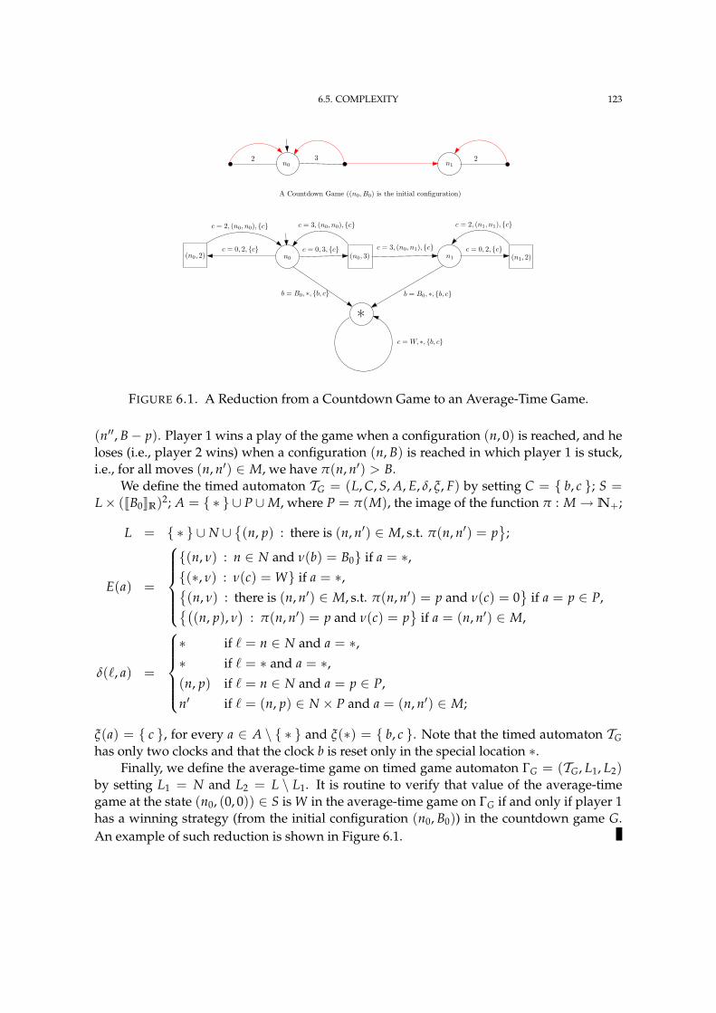
6.5. COMPLEXITY 123
n0 n12 3 2
A Countdown Game ((n0, B0) is the initial configuration)
(n0, 2) n0 (n0, 3) n1 (n1, 2)
*
c = 0, 2, c c = 0, 3, c c = 0, 2, c
c = 2, (n0, n0), c c = 3, (n0, n0), c c = 2, (n1, n1), c
b = B0, ∗, b, c b = B0, ∗, b, c
c = 3, (n0, n1), c
c = W, ∗, b, c
FIGURE 6.1. A Reduction from a Countdown Game to an Average-Time Game.
(n′′, B− p). Player 1 wins a play of the game when a configuration (n, 0) is reached, and heloses (i.e., player 2 wins) when a configuration (n, B) is reached in which player 1 is stuck,i.e., for all moves (n, n′) ∈ M, we have π(n, n′) > B.
We define the timed automaton TG = (L, C, S, A, E, δ, ξ, F) by setting C = b, c ; S =L× (JB0KR)2; A = ∗ ∪ P ∪M, where P = π(M), the image of the function π : M→N+;
L = ∗ ∪ N ∪(n, p) : there is (n, n′) ∈ M, s.t. π(n, n′) = p
;
E(a) =
(n, ν) : n ∈ N and ν(b) = B0 if a = ∗,(∗, ν) : ν(c) = W if a = ∗,(n, ν) : there is (n, n′) ∈ M, s.t. π(n, n′) = p and ν(c) = 0
if a = p ∈ P,(
(n, p), ν)
: π(n, n′) = p and ν(c) = p
if a = (n, n′) ∈ M,
δ(`, a) =
∗ if ` = n ∈ N and a = ∗,∗ if ` = ∗ and a = ∗,(n, p) if ` = n ∈ N and a = p ∈ P,
n′ if ` = (n, p) ∈ N × P and a = (n, n′) ∈ M;
ξ(a) = c , for every a ∈ A \ ∗ and ξ(∗) = b, c . Note that the timed automaton TGhas only two clocks and that the clock b is reset only in the special location ∗.
Finally, we define the average-time game on timed game automaton ΓG = (TG, L1, L2)by setting L1 = N and L2 = L \ L1. It is routine to verify that value of the average-timegame at the state (n0, (0, 0)) ∈ S is W in the average-time game on ΓG if and only if player 1has a winning strategy (from the initial configuration (n0, B0)) in the countdown game G.An example of such reduction is shown in Figure 6.1.
Part 3
Conclusion
7Summary and Future Work
7.1. Summary
In this thesis we presented a study of competitive optimisation on timed automata. Weintroduced an important class of strategies, boundary strategies, that suggest to a playera symbolic timed move of the form (b, c, a)— “wait until the value of the clock c is in veryclose proximity of the integer b, and then execute a transition labelled with the action a”. Theexistence of optimal boundary strategies for a competitive optimisation problem allows usto work with the boundary region graph abstraction of the timed automata, which—for afixed initial state—is a finite graph. Hence, to solve competitive optimisation problems ontimed automata, it is sufficient to prove that there exist optimal boundary strategies for bothplayers, and to then solve the corresponding optimisation problems on finite subgraphs ofreachable states of the boundary region graph.
We showed that for a number of non-competitive optimisation problems and forcompetitive optimisation problems with reachability time and average time objectives thereexist optimal boundary strategies.
For a noncompetitive optimisation problem on concavely-priced timed automata opti-mal boundary strategies exists if the corresponding cost function is a concave-regular func-tion. Concave-regularity is satisfied by a number of cost functions including reachability-price, average-time, average-price, and average price-per-time-unit. The decision versionof optimisation problems for a concave-regular cost function is PSPACE-complete on timedautomata with at least three clocks.
Using Bellman’s optimality equations, we showed that reachability-time games arepositionally determined, and that in reachability-time games optimal boundary strategiesexist for both players. We presented a strategy improvement algorithm to solve theseoptimality equations. We showed that the complexity of solving reachability-time gamesis EXPTIME-complete for timed automata with at least two clocks.
Using closed region graph, an abstraction of timed automata, we showed that average-time games are determined, and that in average-time games optimal boundary strategiesexist for both players. We showed that the complexity of solving average-time games isEXPTIME-complete for timed automata with at least two clocks.
125
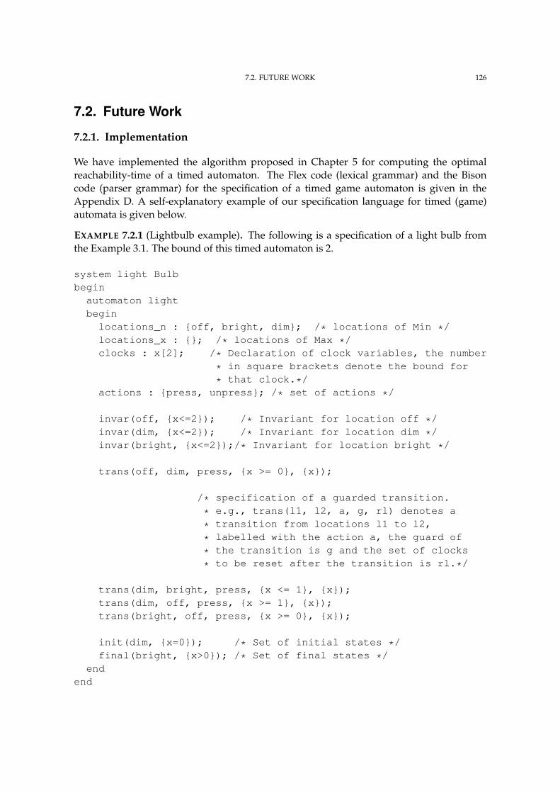
7.2. FUTURE WORK 126
7.2. Future Work
7.2.1. Implementation
We have implemented the algorithm proposed in Chapter 5 for computing the optimalreachability-time of a timed automaton. The Flex code (lexical grammar) and the Bisoncode (parser grammar) for the specification of a timed game automaton is given in theAppendix D. A self-explanatory example of our specification language for timed (game)automata is given below.
EXAMPLE 7.2.1 (Lightbulb example). The following is a specification of a light bulb fromthe Example 3.1. The bound of this timed automaton is 2.
system light Bulbbegin
automaton lightbeginlocations_n : off, bright, dim; /* locations of Min */locations_x : ; /* locations of Max */clocks : x[2]; /* Declaration of clock variables, the number
* in square brackets denote the bound for
* that clock.*/actions : press, unpress; /* set of actions */
invar(off, x<=2); /* Invariant for location off */invar(dim, x<=2); /* Invariant for location dim */invar(bright, x<=2);/* Invariant for location bright */
trans(off, dim, press, x >= 0, x);
/* specification of a guarded transition.
* e.g., trans(l1, l2, a, g, rl) denotes a
* transition from locations l1 to l2,
* labelled with the action a, the guard of
* the transition is g and the set of clocks
* to be reset after the transition is rl.*/
trans(dim, bright, press, x <= 1, x);trans(dim, off, press, x >= 1, x);trans(bright, off, press, x >= 0, x);
init(dim, x=0); /* Set of initial states */final(bright, x>0); /* Set of final states */
endend
7.2. FUTURE WORK 127
The computational complexity of reachability-time games (EXPTIME-complete) indi-cates that it is unlikely to have an efficient algorithm for this problem. Our implementationof the strategy improvement algorithm for the reachability-time games is inefficient: itconstructs and stores the whole boundary region graph of the timed automaton underconsideration. More work is needed to make this implementation of practical interest.
A possible future direction of research work is to investigate symbolic zone-basedalgorithms [UPP] for competitive optimisation problems studied in this thesis.
7.2.2. Complexity of Competitive Optimisation Problems for Timed Automatawith Two Clocks
The exact complexity of the reachability problem on timed automata with two clocks isunknown. By the time-abstract bisimulation property of region equivalence relation, itfollows that the problem is in PSPACE. Laroussinie, Markey, and Schnoebelen [LMS04]proved the NP-hardness by giving a reduction from NP-complete subset-sum problem toreachability problem on timed automata with two clocks.
Using countdown games [JLS07], we proved that reachability games on timed au-tomata with two clocks are EXPTIME-hard. Our initial guess was to use a similarapproach—first prove that one-player countdown games are PSPACE-complete and thengive a reduction from one-player countdown games to reachability problem on timedautomata with two clocks—to prove PSPACE-hardness of this problem. However, oneplayer countdown games turned out to be NP-complete.
The question of the exact complexity of the reachability problem, and hence of allthe other one-player optimisation problems (reachability price, discounted price, averageprice, price-per-reward average, etc.) on concavely-priced timed automata with two clocksremains open.
However, for timed automata with one clock we can generalise the construction ofLaroussinie, Markey, and Schnoebelen [LMS04]—which they used to show NLOGSPACE-membership of the reachability problem for one clock timed automata—to obtain anabstraction similar to the boundary region graph whose size is polynomial in the size oftimed automata. Using such abstraction and the techniques presented in this thesis, itcan be shown that for one clock timed automata noncompetitive optimisation problemsfor concave-regular cost functions are in NLOGSPACE. Similarly it is easy to show that forone-clock timed automata reachability-time games are in PTIME, and average-time gamesare in NP ∩ co-NP.
7.2.3. Maximisation Problem on Concave-Priced Timed Automata
In Chapter 4 we showed that minimisation problems on concavely-priced timed automatafor concave-regular cost functions are PSPACE-complete. Using similar arguments it can beshown that maximisation problems on convexly-priced timed automata for convex-regularcost functions are PSPACE-complete.
We do not know much about maximisation problem on concavely-priced timedautomata. However, for the following class of cost functions, it can easily be shown that
7.2. FUTURE WORK 128
both maximisation and minimisation problems on concavely-priced timed automata arePSPACE-complete, as a monotonic function is both quasiconcave and quasiconvex [BV04].
DEFINITION 7.2.2 (Monotonic-Regular Cost Function). A cost function Cost : PreRuns→ R
is monotonic-regular if it satisfies the following properties.(1) (Monotonicity). For every region R ∈ R and for every run type Λ ∈ Types(R), there
is N ∈ N, such that for every state s ∈ R and for every n ≥ N, the function CostΛn,sis monotonic on ∆Λ
n,s.(2) (Regular Lipschitz-continuity). There is a constant κ ≥ 0, such that for every region
R ∈ R and for every positional run type Λ ∈ Types(R), there is N ∈N, such that forevery state s ∈ R and for every n ≥ N, the function CostΛn,s is κ-continuous on ∆Λ
n,s.(3) (Positional optimality). There is a positional optimal strategy for Cost in T .(4) (Uniform convergence). For every s ∈ S we have that
CostT∗ (s, [s]) = limn→∞
CostTn,∗(s, [s]).
7.2.4. Optimisation on Probabilistic Timed Automata
In this thesis, we considered competitive optimisation problem for the systems having time-critical behaviours modelled using timed automata. One possible direction for the futurework in this line of research is to extend these techniques to solve competitive optimisationproblems for systems having both time-critical and probabilistic behaviours.
Markov decision processes (MDPs) extend finite automata by providing a probabilitydistribution on the successor states for every transition. Timed automata, as we discussedin this thesis, extend finite automata by providing a mechanism to constrain the transitionswith continuous time. Probabilistic timed automata—a hybrid between MDPs and timedautomata—were suggested by Kwiatkowska et al. [KNSS99] as a modelling formalismfor system exhibiting both timed and probabilistic characteristics. We propose the studyof optimisation problems (expected reachability-price, expected discounted-price, andexpected average-price) on concavely-priced probabilistic timed automata which, arguably,can be used to model a larger class of scheduling problems than MDPs, concavely-pricedtimed automata and probabilistic timed automata.
We conjecture that optimisation problems for these three objectives are decidable. Weclaim that an abstraction—let us call it boundary region MDP—similar to boundary regiongraph extended with probability distribution on the edges may be suitable to solve theseoptimisation problems on probabilistic timed automata.
Part 4
Appendix
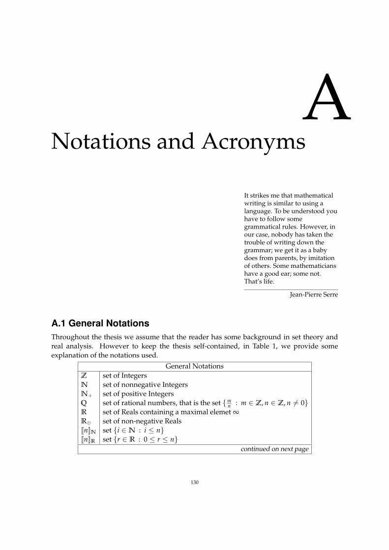
ANotations and Acronyms
It strikes me that mathematicalwriting is similar to using alanguage. To be understood youhave to follow somegrammatical rules. However, inour case, nobody has taken thetrouble of writing down thegrammar; we get it as a babydoes from parents, by imitationof others. Some mathematicianshave a good ear; some not.That’s life.
Jean-Pierre Serre
A.1 General NotationsThroughout the thesis we assume that the reader has some background in set theory andreal analysis. However to keep the thesis self-contained, in Table 1, we provide someexplanation of the notations used.
General NotationsZ set of IntegersN set of nonnegative IntegersN+ set of positive IntegersQ set of rational numbers, that is the set m
n : m ∈ Z, n ∈ Z, n 6= 0R set of Reals containing a maximal elemet ∞R⊕ set of non-negative RealsJnKN set i ∈N : i ≤ nJnKR set r ∈ R : 0 ≤ r ≤ n
continued on next page
130
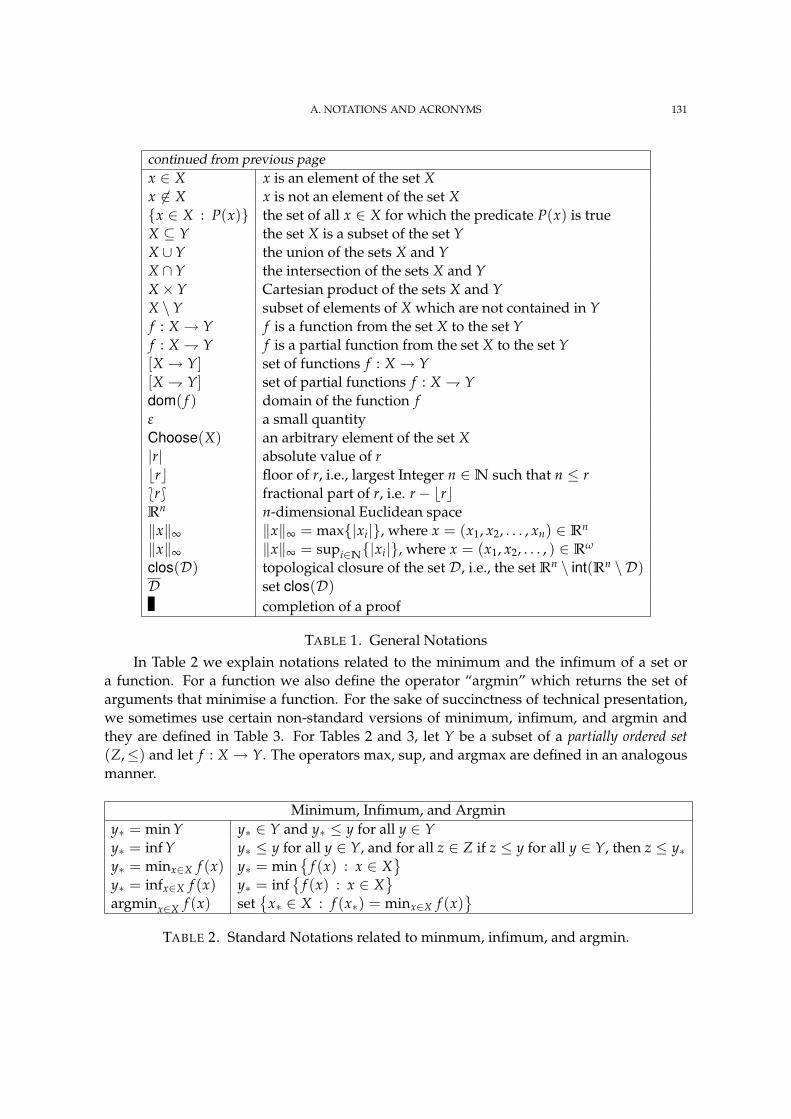
A. NOTATIONS AND ACRONYMS 131
continued from previous pagex ∈ X x is an element of the set Xx 6∈ X x is not an element of the set Xx ∈ X : P(x) the set of all x ∈ X for which the predicate P(x) is trueX ⊆ Y the set X is a subset of the set YX ∪Y the union of the sets X and YX ∩Y the intersection of the sets X and YX×Y Cartesian product of the sets X and YX \Y subset of elements of X which are not contained in Yf : X → Y f is a function from the set X to the set Yf : X Y f is a partial function from the set X to the set Y[X → Y] set of functions f : X → Y[X Y] set of partial functions f : X Ydom( f ) domain of the function fε a small quantityChoose(X) an arbitrary element of the set X|r| absolute value of rbrc floor of r, i.e., largest Integer n ∈N such that n ≤ r*r+ fractional part of r, i.e. r− brcRn n-dimensional Euclidean space‖x‖∞ ‖x‖∞ = max|xi|, where x = (x1, x2, . . . , xn) ∈ Rn
‖x‖∞ ‖x‖∞ = supi∈N|xi|, where x = (x1, x2, . . . , ) ∈ Rω
clos(D) topological closure of the set D, i.e., the set Rn \ int(Rn \ D)D set clos(D)
completion of a proof
TABLE 1. General NotationsIn Table 2 we explain notations related to the minimum and the infimum of a set or
a function. For a function we also define the operator “argmin” which returns the set ofarguments that minimise a function. For the sake of succinctness of technical presentation,we sometimes use certain non-standard versions of minimum, infimum, and argmin andthey are defined in Table 3. For Tables 2 and 3, let Y be a subset of a partially ordered set(Z,≤) and let f : X → Y. The operators max, sup, and argmax are defined in an analogousmanner.
Minimum, Infimum, and Argminy∗ = min Y y∗ ∈ Y and y∗ ≤ y for all y ∈ Yy∗ = inf Y y∗ ≤ y for all y ∈ Y, and for all z ∈ Z if z ≤ y for all y ∈ Y, then z ≤ y∗y∗ = minx∈X f (x) y∗ = min
f (x) : x ∈ X
y∗ = infx∈X f (x) y∗ = inf
f (x) : x ∈ X
argminx∈X f (x) set
x∗ ∈ X : f (x∗) = minx∈X f (x)
TABLE 2. Standard Notations related to minmum, infimum, and argmin.
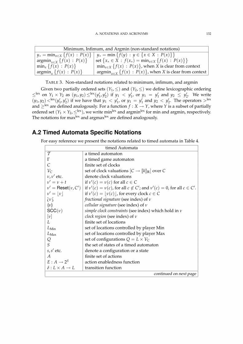
A. NOTATIONS AND ACRONYMS 132
Minimum, Infimum, and Argmin (non-standard notations)y∗ = minx∈X
f (x) : P(x)
y∗ = min
f (y) : y ∈
x ∈ X : P(x)
argminx∈X
f (x) : P(x)
set
x∗ ∈ X : f (x∗) = minx∈X
f (x) : P(x)
minx
f (x) : P(x)
minx∈X
f (x) : P(x)
, when X is clear from contextargminx
f (x) : P(x)
argminx∈X
f (x) : P(x)
, when X is clear from context
TABLE 3. Non-standard notations related to minimum, infimum, and argminGiven two partially ordered sets (Y1,≤) and (Y2,≤) we define lexicographic ordering
≤lex on Y1 × Y2 as (y1, y2)≤lex(y′1, y′2) if y1 < y′1, or y1 = y′1 and y2 ≤ y′2. We write(y1, y2) <lex(y′1, y′2) if we have that y1 < y′1, or y1 = y′1 and y2 < y′2. The operators >lex
and ≥lex are defined analogously. For a function f : X → Y, where Y is a subset of partiallyordered set (Y1 × Y2,≤lex), we write minlex and argminlex for min and argmin, respectively.The notations for maxlex and argmaxlex are defined analogously.
A.2 Timed Automata Specific NotationsFor easy reference we present the notations related to timed automata in Table 4.
timed AutomataT a timed automatonΓ a timed game automatonC finite set of clocksVC set of clock valuations [C → JkKR] over Cν, ν′ etc. denote clock valuationsν′ = ν + t if ν′(c) = ν(c) for all c ∈ Cν′ = Reset(ν, C′) if ν′(c) = ν(c), for all c 6∈ C′; and ν′(c) = 0, for all c ∈ C′.ν′ = bνc if ν′(c) = bν(c)c, for every clock c ∈ CHνI fractional signature (see index) of ν
LνM cellular signature (see index) of ν
SCC(ν) simple clock constraints (see index) which hold in ν
[ν] clock region (see index) of ν
L finite set of locationsLMin set of locations controlled by player MinLMax set of locations controlled by player MaxQ set of configurations Q = L× VCS the set of states of a timed automatons, s′ etc. denote a configuration or a stateA finite set of actionsE : A→ 2S action enabledness functionδ : L× A→ L transition function
continued on next page
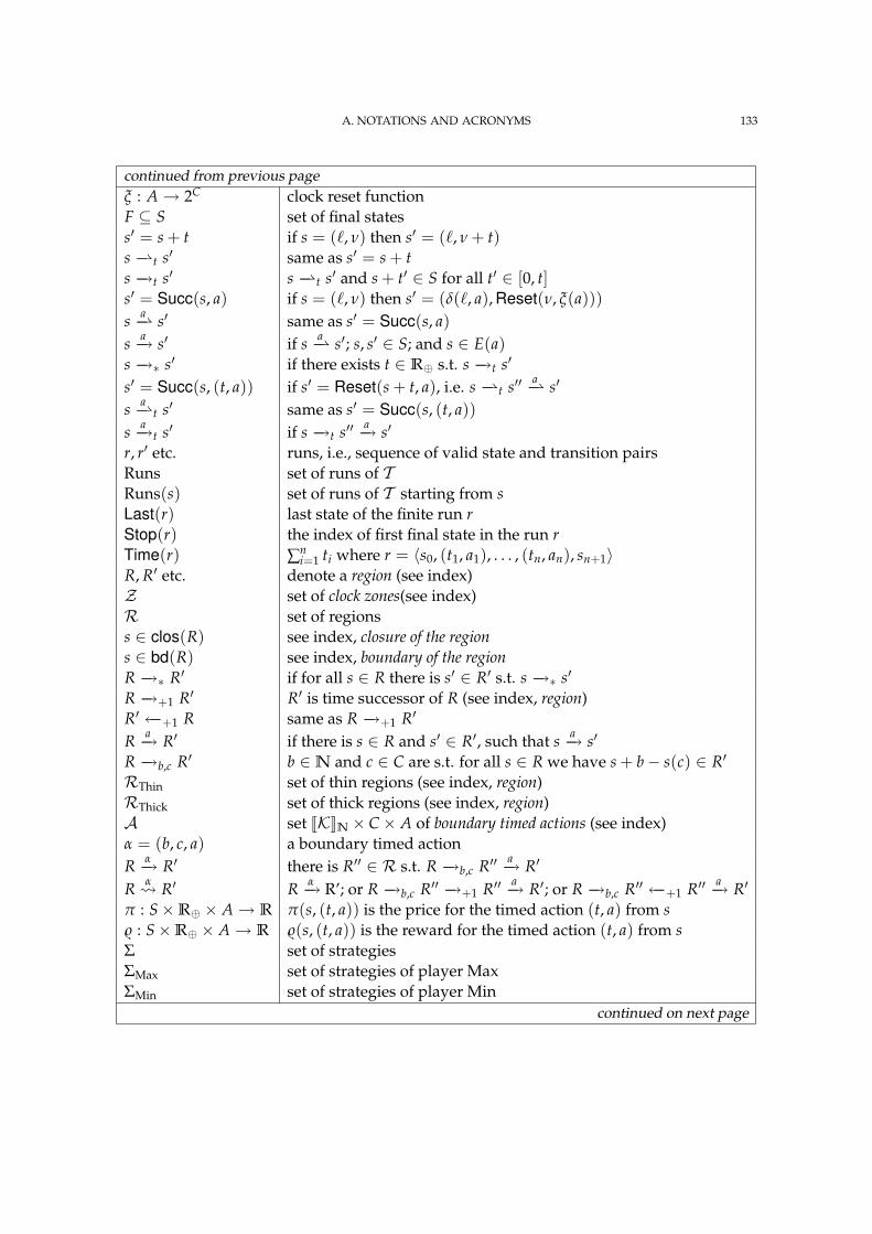
A. NOTATIONS AND ACRONYMS 133
continued from previous pageξ : A→ 2C clock reset functionF ⊆ S set of final statess′ = s + t if s = (`, ν) then s′ = (`, ν + t)s −t s′ same as s′ = s + ts −→t s′ s −t s′ and s + t′ ∈ S for all t′ ∈ [0, t]s′ = Succ(s, a) if s = (`, ν) then s′ = (δ(`, a), Reset(ν, ξ(a)))s a− s′ same as s′ = Succ(s, a)s a−→ s′ if s a− s′; s, s′ ∈ S; and s ∈ E(a)s −→∗ s′ if there exists t ∈ R⊕ s.t. s −→t s′
s′ = Succ(s, (t, a)) if s′ = Reset(s + t, a), i.e. s −t s′′ a− s′
s a−t s′ same as s′ = Succ(s, (t, a))s a−→t s′ if s −→t s′′ a−→ s′
r, r′ etc. runs, i.e., sequence of valid state and transition pairsRuns set of runs of TRuns(s) set of runs of T starting from sLast(r) last state of the finite run rStop(r) the index of first final state in the run rTime(r) ∑n
i=1 ti where r = 〈s0, (t1, a1), . . . , (tn, an), sn+1〉R, R′ etc. denote a region (see index)Z set of clock zones(see index)R set of regionss ∈ clos(R) see index, closure of the regions ∈ bd(R) see index, boundary of the regionR −→∗ R′ if for all s ∈ R there is s′ ∈ R′ s.t. s −→∗ s′
R −→+1 R′ R′ is time successor of R (see index, region)R′ ←−+1 R same as R −→+1 R′
R a−→ R′ if there is s ∈ R and s′ ∈ R′, such that s a−→ s′
R −→b,c R′ b ∈N and c ∈ C are s.t. for all s ∈ R we have s + b− s(c) ∈ R′
RThin set of thin regions (see index, region)RThick set of thick regions (see index, region)A set JKKN × C× A of boundary timed actions (see index)α = (b, c, a) a boundary timed actionR α−→ R′ there is R′′ ∈ R s.t. R −→b,c R′′ a−→ R′
R α R′ R α−→ R’; or R −→b,c R′′ −→+1 R′′ a−→ R′; or R −→b,c R′′ ←−+1 R′′ a−→ R′
π : S×R⊕ × A→ R π(s, (t, a)) is the price for the timed action (t, a) from s$ : S×R⊕ × A→ R $(s, (t, a)) is the reward for the timed action (t, a) from sΣ set of strategiesΣMax set of strategies of player MaxΣMin set of strategies of player Min
continued on next page
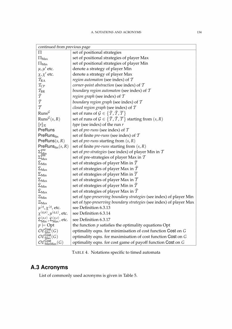
A. NOTATIONS AND ACRONYMS 134
continued from previous pageΠ set of positional strategiesΠMax set of positional strategies of player MaxΠMin set of positional strategies of player Minµ, µ′ etc. denote a strategy of player Minχ, χ′ etc. denote a strategy of player MaxTRA region automaton (see index) of TTCP corner-point abstraction (see index) of TTBR boundary region automaton (see index) of TT region graph (see index) of TT boundary region graph (see index) of TT closed region graph (see index) of TRunsG set of runs of G ∈
T , T , T
RunsG(s, R) set of runs of G ∈
T , T , T
starting from (s, R)
JrKR type (see index) of the run rPreRuns set of pre-runs (see index) of TPreRunsfin set of finite pre-runs (see index) of TPreRuns(s, R) set of pre-runs starting from (s, R)PreRunsfin(s, R) set of finite pre-runs starting from (s, R)Σpre
Min set of pre-strategies (see index) of player Min in TΣpre
Max set of pre-strategies of player Max in TΣMin set of strategies of player Min in TΣMax set of strategies of player Max in TΣMin set of strategies of player Min in TΣMax set of strategies of player Max in TΣMin set of strategies of player Min in TΣMax set of strategies of player Max in TΞMin set of type-preserving boundary strategies (see index) of player MinΞMax set of type-preserving boundary strategies (see index) of player Maxµ↓q, χ↓q, etc. see Definition 6.3.13χ(q,µ), µ(q,χ), etc. see Definition 6.3.14Σ(µ,ε)
Min , Σ(χ,ε)Max , etc. see Definition 6.3.17
p |= Opt the function p satisfies the optimality equations OptOECost
Min (G) optimality eqns. for minimisation of cost function Cost on GOECost
Max (G) optimality eqns. for maximisation of cost function Cost on GOECost
MinMax(G) optimality eqns. for cost game of payoff function Cost on G
TABLE 4. Notations specific to timed automata
A.3 AcronymsList of commonly used acronyms is given in Table 5.
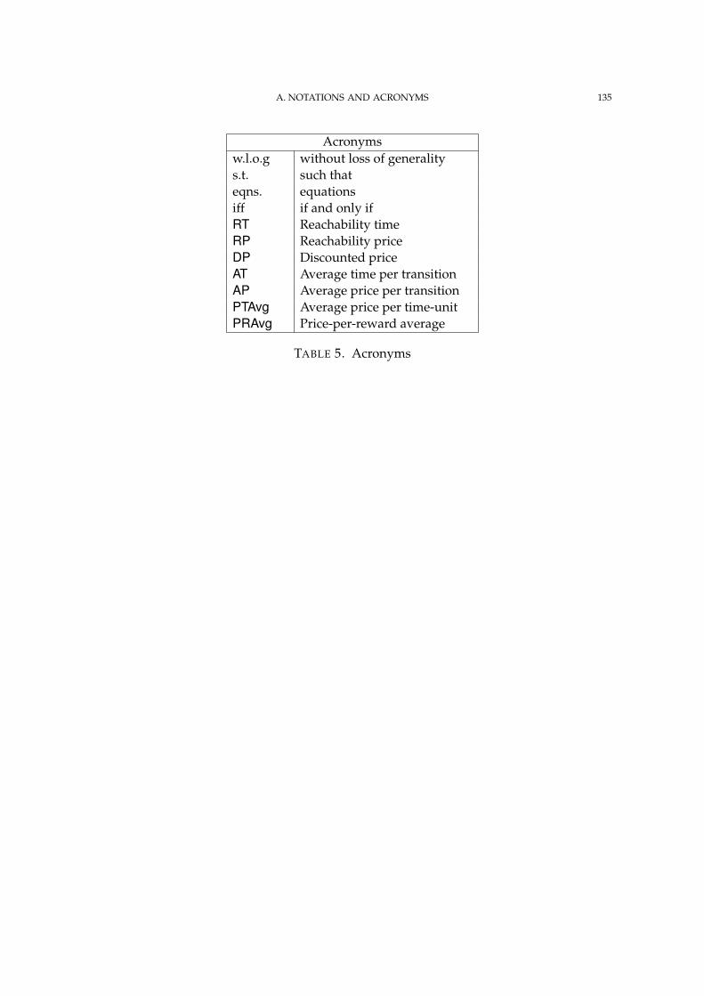
A. NOTATIONS AND ACRONYMS 135
Acronymsw.l.o.g without loss of generalitys.t. such thateqns. equationsiff if and only ifRT Reachability timeRP Reachability priceDP Discounted priceAT Average time per transitionAP Average price per transitionPTAvg Average price per time-unitPRAvg Price-per-reward average
TABLE 5. Acronyms
BResults From Real Analysis
Indeed, I have found a very niceway of expressing continuity . . .
Rudolph Lipschitz
B.1. Lipschitz-Continuous FunctionsA function f : Rn → Rm is Lipschitz-continuous [EEJ04] on its domain dom( f ), if thereexists a constant K ≥ 0, called a Lipschitz constant of f , such that ‖ f (x)− f (y)‖ ≤ K‖x− y‖for all x, y ∈ dom( f ); we then also say that f is K-continuous. A K-continuous function iscontraction if K < 1.
The following properties [EEJ04] of Lipschitz-continuous functions are of interest inthis thesis.
LEMMA B.1.1. If for every i = 1, 2, . . . , k, the function fi : Rn → Rm is Ki-continuous andwi ∈ R, then the function Rn 3 x 7→ ∑n
i=1 wi fi(x) is K-continuous for K = ∑ki=1 |wi|Ki.
PROOF. Let x, y ∈ Rn and assume that for every i = 1, 2, . . . , k, the function fi : Rn → Rm
is Ki-continuous.
| f (x)− f (y)| =∣∣∣∣∣ k
∑i=0
wi · fi(x)−k
∑i=0
wi · fi(y)
∣∣∣∣∣ =
∣∣∣∣∣ k
∑i=0
(wi · ( fi(x)− fi(y)))
∣∣∣∣∣≤
k
∑i=0
(|wi · ( fi(x)− fi(y)))| ≤k
∑i=0
(|wi| · Ki · |x− y|) =k
∑i=0
(|wi| · Ki) · |x− y|
The first, the second, and the last equalities are straightforward. The first inequality followsas |a + b| ≤ |a|+ |b|, and the last inequality holds as the function fi is Ki-continuous for alli = 1, 2, . . . , k.
LEMMA B.1.2. If f1 : Rn → Rm and f2 : Rm → Rk are K1-continuous and K2-continuous,respectively, then their composition, Rn 3 x 7→ f2( f1(x)), is K-continuous for K = K1K2.
PROOF. Let x, y ∈ Rn, and assume that f1 and f2 are K1-continuous and K2-continuous,respectively.
| f (x)− f (y)| = | f2( f1(x))− f2( f1(y))| ≤ K2 · | f1(x)− f1(y)| ≤ K2 · K1 · |x− y|136
B.2. CONCAVE AND QUASICONCAVE FUNCTIONS 137
The first inequality follows from K2-continuity of f2 and the last inequality follows fromK1-continuity of f1.
LEMMA B.1.3. Let f1, f2 : Rn → R be K1-continuous and K2-continuous, respectively; letf1 and f2 be bounded, i.e., there is a constant M ≥ 0, such that for all x ∈ dom( f1) ∩dom( f2), we have | f1(x)|, | f2(x)| ≤ M; and let f2 be bounded from below, i.e., there is aconstant N > 0, such that for all x ∈ dom( f2), we have f2(x) ≥ N. Then the functionRn 3 x 7→ f1(x)/ f2(x) is K-continuous for K = (NK1 + MK2)/N2.
PROOF. Let x, y ∈ Rn, and assume that f1 and f2 are K1-continuous and K2-continuous,respectively. Further assume that f1 and f2 are bounded by M, and that f2 is bounded frombelow by N > 0.
| f (x)− f (y)| =∣∣∣∣ f1(x)
f2(x)− f1(y)
f2(y)
∣∣∣∣ =∣∣∣∣ f1(x) f2(y)− f1(y) f2(x)
f2(x) f2(y)
∣∣∣∣=∣∣∣∣ f1(x) f2(y)− f2(y) f1(y) + f2(y) f1(y)− f1(y) f2(x)
f2(x) f2(y)
∣∣∣∣=∣∣∣∣ f2(y)( f1(x)− f1(y)) + f1(y)( f2(y)− f2(x))
f2(x) f2(y)
∣∣∣∣≤∣∣∣∣ 1
f2(x)
∣∣∣∣ · K1 · |x− y|+∣∣∣∣ f1(y)
f2(x) f2(y)
∣∣∣∣ · K2 · |x− y|
≤ K1
N· |x− y|+ K2 ·M
N2 · |x− y| =(
K1 · N + K2 ·MN2
)· |x− y|
The first inequality follows from Lipschitz-continuity of f1 and f2 and the second inequalityfollows from boundedness assumptions. All the equalities are trivial.
B.2. Concave and Quasiconcave Functions
B.2.1. Concave Functions
A set D ⊆ Rn is convex if for all x, y ∈ D and λ ∈ [0, 1], we have λx + (1− λ)y ∈ D. Afunction f : Rn → R is concave (on its domain dom( f ) ⊆ Rn), if dom( f ) ⊆ Rn is a convexset, and for all x, y ∈ Rn and λ ∈ [0, 1], we have f (λx + (1− λ)y) ≥ λ f (x) + (1− λ) f (y).A function f is convex if the function − f is concave. A function is affine if it is both convexand concave.
The α-superlevel set of a function f : Rn → R is defined as Sα( f ) = x ∈ dom( f ) :f (x) ≥ α, and the α-sublevel set of f is defined as Sα( f ) = x ∈ dom( f ) : f (x) ≤ α.PROPOSITION B.2.1 ([BV04]). If a function is concave then its superlevel sets are convex;and if it is convex then its sublevel sets are convex.
The following properties [BV04] of concave functions are of interest in this thesis.
B.2. CONCAVE AND QUASICONCAVE FUNCTIONS 138
LEMMA B.2.2 (Non-negative weighted sum). If f1, f2, . . . , fk : Rn → R are concave andw1, w2, . . . , wk ≥ 0, then their weighted sum Rn 3 x 7→ ∑k
i=1 wi · fi is concave on its domain⋂ki=1 dom( fi).
PROOF. Let x, y ∈ Rn, λ ∈ [0, 1], and f1, f2, . . . , fk are concave.
f (λx + (1− λ)y)) =n
∑i=1
wi · fi(λx + (1− λ)y) ≥n
∑i=1
wi · (λ fi(x) + (1− λ) fi(y))
= λn
∑i=1
wi · fi(x) + (1− λ)n
∑i=1
wi · fi(y) = λ f (x) + (1− λ) f (y).
The inequality follows from the concavity assumption, and the equalities are straight-forward.
LEMMA B.2.3 (Composition with affine function). If f : Rn → R is concave and g : Rm →Rn is affine, then their composition Rn 3 x 7→ f (g(x)) if concave.
PROOF. Let x, y ∈ Rn and λ ∈ [0, 1]. Also, assume that f is concave and g is affine.
f (g(λx + (1 − λ)y)) = f (λg(x) + (1 − λ)g(y)) ≥ λ f (g(x)) + (1 − λ) f (g(y)).
The equality follows as g is affine, and the inequality is by concavity of f .
LEMMA B.2.4 (Pointwise minimum). If functions f1, f2, . . . fk : Rn → R are concave, thentheir pointwise minimum Rn 3 x 7→ mink
i=1 fi(x) is concave (on its domain⋂k
i=1 dom( fi)).
PROOF. Let us assume that f1, f2, . . . , fk are concave. Let x, y ∈ Rn and λ ∈ [0, 1].
f (λx + (1− λ)y)) =n
mini=1
fi(λx + (1− λ)y)) ≥n
mini=1
(λ fi(x) + (1− λ) fi(y))
≥ λn
mini=1
fi(x) + (1− λ)n
mini=1
fi(y) = λ f (x) + (1− λ) f (y)
The first inequality holds since, for all i = 1, 2, . . . , k, the function fi is concave, and thesecond inequality follows from that fact that for arbitrary sequences 〈ai〉ni=1 and 〈bi〉ni=1 wehave mini≤n(ai + bi) ≥ mini≤n ai + mini≤n bi.
The proof of the following lemma is similar to the proof of Lemma B.2.4, and henceomitted.
LEMMA B.2.5 (Pointwise infimum). Let f : Rn × Z → R, where Z is an arbitrary(infinite) set. If for all z ∈ Z, the function Rn 3 x 7→ f (x, z) is concave, then the functionRn 3 x 7→ infz∈Z f (x, z) is concave (on its domain
⋂z∈Z dom( f (·, z))).
B.3. FIXED POINT THEOREMS 139
B.2.2. Quasiconcave Functions
A function f : Rn → R is quasiconcave (on its domain dom( f ) ⊆ Rn), if dom( f ) is a convexset, and for all x, y ∈ dom( f ) and λ ∈ [0, 1], we have f (λx + (1− λ)y) ≥ min f (x), f (y).A function f is quasiconvex if the function − f is quasiconcave.
PROPOSITION B.2.6 ([BV04]). A function is quasiconcave if and only if its superlevel setsare convex; and it is quasiconvex if and only if its sublevel sets are convex.
The following properties (see, Mangasarian [Man69]) of quasiconcave functions are ofinterest in this thesis.
LEMMA B.2.7 (Quasiconcavity of ratio functions). For h1, h2 : Rn → R, the functionRn 3 x 7→ h1(x)/h2(x) is quasiconcave (on its domain dom(h1) ∩ dom(h2)) if at least oneof the following holds:
(1) h1 is nonnegative and concave, h2 is positive and convex.(2) h1 is nonpositive and concave, h2 is positive and concave(3) h1 is nonnegative and convex, h2 is negative and convex.(4) h1 is nonpositive and convex, h2 is negative and concave.(5) h1 is affine and h2 is non-zero and affine;(6) h1 is concave, and h2 is positive and affine;(7) h1 is convex, and h2 is negative and affine.
PROOF. To prove that the function f is quasiconcave, it is sufficient to show that thesuperlevel sets of f are convex, i.e. for all α ∈ R we have that the set x : h1(x)
h2(x) ≥ α orequivalently the set x : h1(x)− α · h2(x) ≥ 0 is convex. It is easy to see that is the casewhen either of the above assumptions hold.
B.3. Fixed Point TheoremsWe say that x ∈ X is a fixed point of a function F : X → X if F(x) = x. Before we state twoimportant fixed point theorems, we need to define some concepts.
A metric space is an order pair (X, d) where X is a set and d is a metric on X. Given ametric space (X, d), a sequence 〈x0, x1, . . .〉 is called Cauchy, if for every positive real numberε > 0, there exists N ∈N such that for all natural numbers m, n > N we have d(xm, xn) < ε.A metric space (X, d) in which every Cauchy sequence has a limit in X is called complete.
The following well-known fixed point theorems [KK01] are used in this thesis.
THEOREM B.3.1 (Banach Fixed Point Theorem). Let the function f : X → X be a contractionover a complete metric space (X, d). Then f has a unique fixed-point x0 ∈ X. Moreover, foran y ∈ X, d( f n(y), x0)→ 0 as n→ ∞.
THEOREM B.3.2 (Brouwer’s Fixed Point Theorem). Let X be an nonempty, compact (closedand bounded), convex set in a finite dimensional Euclidean space. Then a continuousmapping f : X → X has at least one fixed point.
CSome Determinacy Results
It’s not hard to make decisionswhen you know what yourvalues are.
Roy Disney
C.1. Matrix GamesA Matrix game Γ = (M) is played on an (m× n) matrix M between two players Max andMin. In this game, player Max chooses a row i of the matrix and player Min chooses acolumn j of the matrix and thus player Max wins 1 M(i, j) from player Min.
Let the set of pure strategies of the player Max be 1, 2, . . . , m and the set of purestrategies set of player Min is 1, 2, . . . , n. The set ΣMax ⊆ Rm of mixed strategies of playerMax as the set of probability distributions over the set of pure strategies. Hence we have(p1, p2, . . . , pm) ∈ ΣMax if and only if ∑m
i=1 pi = 1 and pi ≥ 0 for all 1 ≤ i ≤ m. We define theset ΣMin of mixed strategies of the player Min in an analogous manner.
PROPOSITION C.1.1. In a matrix game the product set ΣMin × ΣMax of the mixed strategysets of players Min and Max is nonempty, compact and convex.
For every index 1 ≤ i ≤ m, we define the strategy χi ∈ ΣMax such that for every index1 ≤ j ≤ m, we have χi(j) = 1 if j = i, and χi(j) = 0 otherwise. The strategies µi for playerMin, for every 1 ≤ i ≤ n, are defined analogously.
If player Max plays according to mixed strategy χ ∈ ΣMax and the player Min playsaccording to mixed strategy µ ∈ ΣMin, then the expected win of player Max is given by thefollowing payoff function P : ΣMin × ΣMax → R:
P(µ, χ) =m
∑i=1
n
∑j=1
χ(i) ·M(i, j) · µ(j).
The following fundamental result about the determinacy of Matrix games is due to Johnvon Neumann [vN28]:
1We always say that player Max wins the amount M(i, j) from player Min upon the selection of (i, j)th entryof the matrix. However, in practice, if M(i, j) is positive then player Max wins that amount from Min; and ifM(i, j) is negative player Min wins |M(i, j)| from player Max.
140
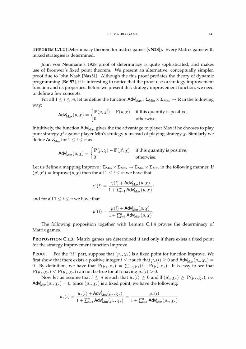
C.1. MATRIX GAMES 141
THEOREM C.1.2 (Determinacy theorem for matrix games [vN28]). Every Matrix game withmixed strategies is determined.
John von Neumann’s 1928 proof of determinacy is quite sophisticated, and makesuse of Brouwer’s fixed point theorem. We present an alternative, conceptually simpler,proof due to John Nash [Nas51]. Although the this proof predates the theory of dynamicprogramming [Bel57], it is interesting to notice that the proof uses a strategy improvementfunction and its properties. Before we present this strategy improvement function, we needto define a few concepts.
For all 1 ≤ i ≤ m, let us define the function AdviMax : ΣMin× ΣMax → R in the following
way:
AdviMax(µ, χ) =
P(µ, χi)−P(µ, χ) if this quantity is positive,
0 otherwise.
Intuitively, the function AdviMax gives the the advantage to player Max if he chooses to play
pure strategy χi against player Min’s strategy µ instead of playing strategy χ. Similarly wedefine Advi
Min for 1 ≤ i ≤ n as
AdviMin(µ, χ) =
P(µ, χ)−P(µi, χ) if this quantity is positive,
0 otherwise.
Let us define a mapping Improve : ΣMin × ΣMax → ΣMin × ΣMax in the following manner. If(µ′, χ′) = Improve(µ, χ) then for all 1 ≤ i ≤ m we have that
χ′(i) =χ(i) + Advi
Max(µ, χ)1 + ∑m
i=1 AdviMax(µ, χ)
;
and for all 1 ≤ i ≤ n we have that
µ′(i) =µ(i) + Advi
Min(µ, χ)1 + ∑n
i=1 AdviMin(µ, χ)
.
The following proposition together with Lemma C.1.4 proves the determinacy ofMatrix games.
PROPOSITION C.1.3. Matrix games are determined if and only if there exists a fixed pointfor the strategy improvement function Improve.
PROOF. For the “if” part, suppose that (µ∗, χ∗) is a fixed point for function Improve. Wefirst show that there exists a positive integer i ≤ n such that µ∗(i) ≥ 0 and Advi
Min(µ∗, χ∗) =0. By definition, we have that P(µ∗, χ∗) = ∑n
i=1 µ∗(i) · P(µi∗, χ∗). It is easy to see that
P(µ∗, χ∗) < P(µi∗, χ∗) can not be true for all i having µ∗(i) > 0.
Now let us assume that i ≤ n is such that µ∗(i) ≥ 0 and P(µi∗, χ∗) ≥ P(µ∗, χ∗), i.e.
AdviMin(µ∗, χ∗) = 0. Since (µ∗, χ∗) is a fixed point, we have the following:
µ∗(i) =µ∗(i) + Advi
Min(µ∗, χ∗)1 + ∑n
i=1 AdviMin(µ∗, χ∗)
=µ∗(i)
1 + ∑ni=1 Advi
Min(µ∗, χ∗)
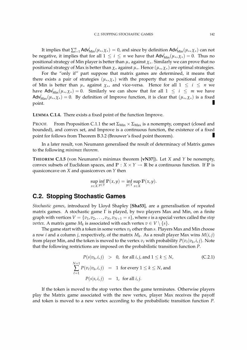
C.2. STOPPING STOCHASTIC GAMES 142
It implies that ∑ni=1 Advi
Min(µ∗, χ∗) = 0, and since by definition AdviMin(µ∗, χ∗) can not
be negative, it implies that for all 1 ≤ i ≤ n we have that AdviMin(µ∗, χ∗) = 0. Thus no
positional strategy of Min player is better than µ∗ against χ∗. Similarly we can prove that nopositional strategy of Max is better than χ∗ against µ∗. Hence (µ∗, χ∗) are optimal strategies.
For the “only if” part suppose that matrix games are determined, it means thatthere exists a pair of strategies (µ∗, χ∗) with the property that no positional strategyof Min is better than µ∗ against χ∗, and vice-versa. Hence for all 1 ≤ i ≤ n wehave Advi
Min(µ∗, χ∗) = 0. Similarly we can show that for all 1 ≤ i ≤ m we haveAdvi
Max(µ∗, χ∗) = 0. By definition of Improve function, it is clear that (µ∗, χ∗) is a fixedpoint.
LEMMA C.1.4. There exists a fixed point of the function Improve.
PROOF. From Proposition C.1.1 the set ΣMin × ΣMax is a nonempty, compact (closed andbounded), and convex set, and Improve is a continuous function, the existence of a fixedpoint for follows from Theorem B.3.2 (Brouwer’s fixed point theorem).
In a later result, von Neumann generalised the result of determinacy of Matrix gamesto the following minimax theorem.
THEOREM C.1.5 (von Neumann’s minimax theorem [vN37]). Let X and Y be nonempty,convex subsets of Euclidean spaces, and P : X × Y → R be a continuous function. If P isquasiconcave on X and quasiconvex on Y then
supx∈X
infy∈Y
P(x, y) = infy∈Y
supx∈X
P(x, y).
C.2. Stopping Stochastic GamesStochastic games, introduced by Lloyd Shapley [Sha53], are a generalisation of repeatedmatrix games. A stochastic game Γ is played, by two players Max and Min, on a finitegraph with vertices V = v1, v2, . . . , vN , vN+1 = s, where s is a special vertex called the stopvertex. A matrix game Mk is associated with each vertex v ∈ V \ s.
The game start with a token in some vertex vk other than s. Players Max and Min choosea row i and a column j, respectively, of the matrix Mk. As a result player Max wins M(i, j)from player Min, and the token is moved to the vertex v` with probability P(v`|vk, i, j). Notethat the following restrictions are imposed on the probabilistic transition function P.
P(s|vk, i, j) > 0, for all i, j, and 1 ≤ k ≤ N, (C.2.1)N+1
∑`=1
P(v`|vk, i, j) = 1 for every 1 ≤ k ≤ N, and
P(s|s, i, j) = 1, for all i, j.
If the token is moved to the stop vertex then the game terminates. Otherwise playersplay the Matrix game associated with the new vertex, player Max receives the payoffand token is moved to a new vertex according to the probabilistic transition function P.
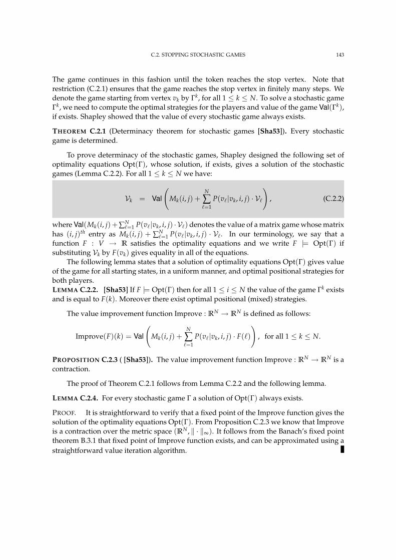
C.2. STOPPING STOCHASTIC GAMES 143
The game continues in this fashion until the token reaches the stop vertex. Note thatrestriction (C.2.1) ensures that the game reaches the stop vertex in finitely many steps. Wedenote the game starting from vertex vk by Γk, for all 1 ≤ k ≤ N. To solve a stochastic gameΓk, we need to compute the optimal strategies for the players and value of the game Val(Γk),if exists. Shapley showed that the value of every stochastic game always exists.
THEOREM C.2.1 (Determinacy theorem for stochastic games [Sha53]). Every stochasticgame is determined.
To prove determinacy of the stochastic games, Shapley designed the following set ofoptimality equations Opt(Γ), whose solution, if exists, gives a solution of the stochasticgames (Lemma C.2.2). For all 1 ≤ k ≤ N we have:
Vk = Val
(Mk(i, j) +
N
∑`=1
P(v`|vk, i, j) · V`
), (C.2.2)
where Val(Mk(i, j)+ ∑N`=1 P(v`|vk, i, j) · V`) denotes the value of a matrix game whose matrix
has (i, j)th entry as Mk(i, j) + ∑N`=1 P(v`|vk, i, j) · V`. In our terminology, we say that a
function F : V → R satisfies the optimality equations and we write F |= Opt(Γ) ifsubstituting Vk by F(vk) gives equality in all of the equations.
The following lemma states that a solution of optimality equations Opt(Γ) gives valueof the game for all starting states, in a uniform manner, and optimal positional strategies forboth players.LEMMA C.2.2. [Sha53] If F |= Opt(Γ) then for all 1 ≤ i ≤ N the value of the game Γk existsand is equal to F(k). Moreover there exist optimal positional (mixed) strategies.
The value improvement function Improve : RN → RN is defined as follows:
Improve(F)(k) = Val
(Mk(i, j) +
N
∑`=1
P(v`|vk, i, j) · F(`)
), for all 1 ≤ k ≤ N.
PROPOSITION C.2.3 ( [Sha53]). The value improvement function Improve : RN → RN is acontraction.
The proof of Theorem C.2.1 follows from Lemma C.2.2 and the following lemma.
LEMMA C.2.4. For every stochastic game Γ a solution of Opt(Γ) always exists.
PROOF. It is straightforward to verify that a fixed point of the Improve function gives thesolution of the optimality equations Opt(Γ). From Proposition C.2.3 we know that Improveis a contraction over the metric space (RN , ‖ · ‖∞). It follows from the Banach’s fixed pointtheorem B.3.1 that fixed point of Improve function exists, and can be approximated using astraightforward value iteration algorithm.
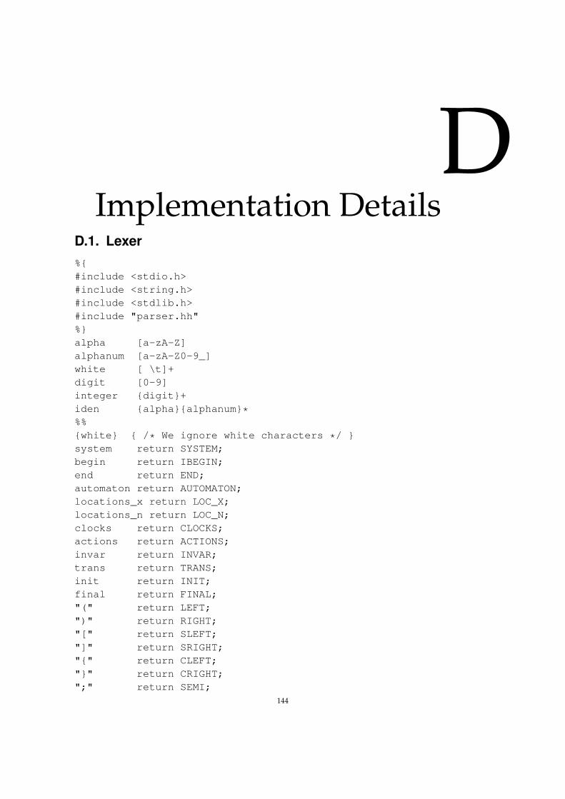
DImplementation Details
D.1. Lexer%#include <stdio.h>#include <string.h>#include <stdlib.h>#include "parser.hh"%alpha [a-zA-Z]alphanum [a-zA-Z0-9_]white [ \t]+digit [0-9]integer digit+iden alphaalphanum*%%white /* We ignore white characters */ system return SYSTEM;begin return IBEGIN;end return END;automaton return AUTOMATON;locations_x return LOC_X;locations_n return LOC_N;clocks return CLOCKS;actions return ACTIONS;invar return INVAR;trans return TRANS;init return INIT;final return FINAL;"(" return LEFT;")" return RIGHT;"[" return SLEFT;"]" return SRIGHT;"" return CLEFT;"" return CRIGHT;";" return SEMI;
144
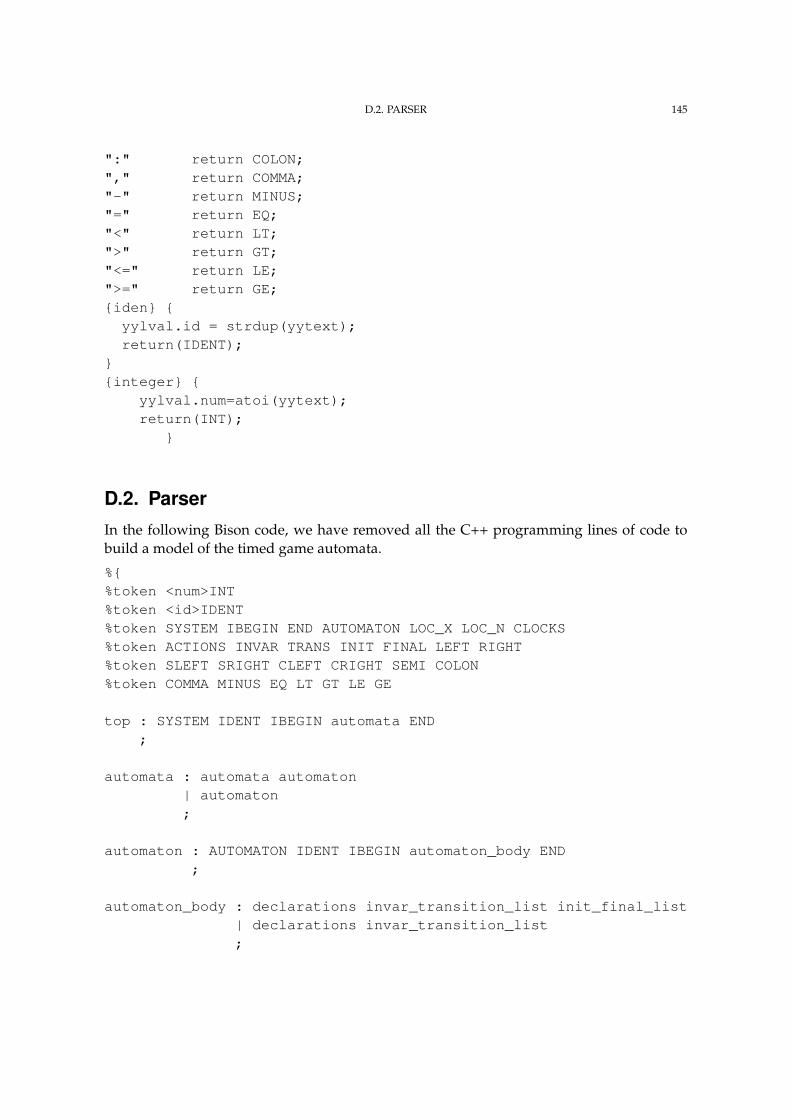
D.2. PARSER 145
":" return COLON;"," return COMMA;"-" return MINUS;"=" return EQ;"<" return LT;">" return GT;"<=" return LE;">=" return GE;iden
yylval.id = strdup(yytext);return(IDENT);
integer
yylval.num=atoi(yytext);return(INT);
D.2. ParserIn the following Bison code, we have removed all the C++ programming lines of code tobuild a model of the timed game automata.
%%token <num>INT%token <id>IDENT%token SYSTEM IBEGIN END AUTOMATON LOC_X LOC_N CLOCKS%token ACTIONS INVAR TRANS INIT FINAL LEFT RIGHT%token SLEFT SRIGHT CLEFT CRIGHT SEMI COLON%token COMMA MINUS EQ LT GT LE GE
top : SYSTEM IDENT IBEGIN automata END;
automata : automata automaton| automaton;
automaton : AUTOMATON IDENT IBEGIN automaton_body END;
automaton_body : declarations invar_transition_list init_final_list| declarations invar_transition_list;
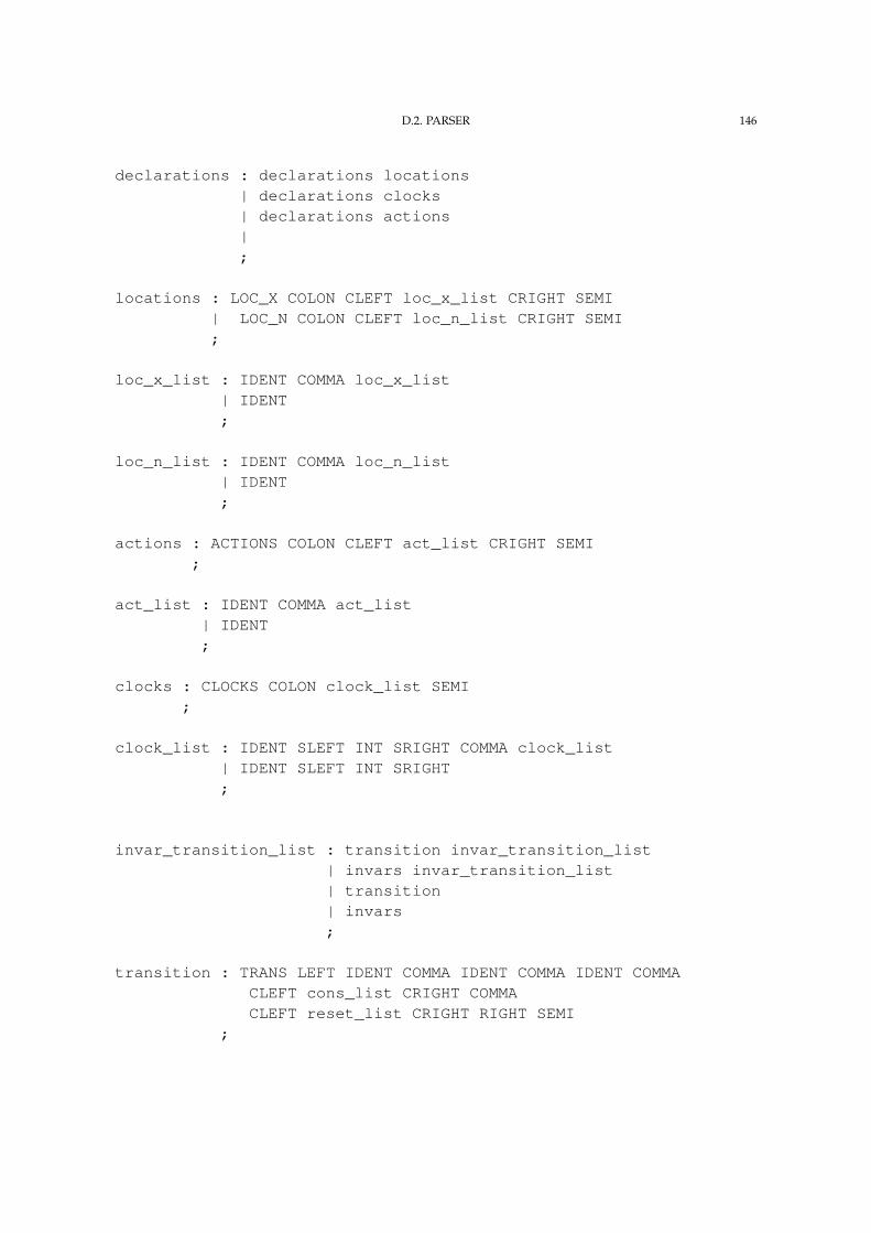
D.2. PARSER 146
declarations : declarations locations| declarations clocks| declarations actions|;
locations : LOC_X COLON CLEFT loc_x_list CRIGHT SEMI| LOC_N COLON CLEFT loc_n_list CRIGHT SEMI;
loc_x_list : IDENT COMMA loc_x_list| IDENT;
loc_n_list : IDENT COMMA loc_n_list| IDENT;
actions : ACTIONS COLON CLEFT act_list CRIGHT SEMI;
act_list : IDENT COMMA act_list| IDENT;
clocks : CLOCKS COLON clock_list SEMI;
clock_list : IDENT SLEFT INT SRIGHT COMMA clock_list| IDENT SLEFT INT SRIGHT;
invar_transition_list : transition invar_transition_list| invars invar_transition_list| transition| invars;
transition : TRANS LEFT IDENT COMMA IDENT COMMA IDENT COMMACLEFT cons_list CRIGHT COMMACLEFT reset_list CRIGHT RIGHT SEMI
;
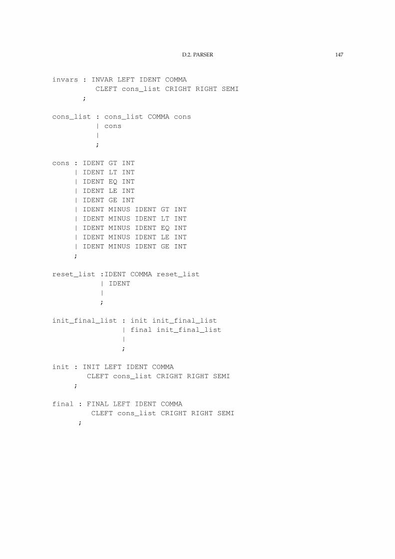
D.2. PARSER 147
invars : INVAR LEFT IDENT COMMACLEFT cons_list CRIGHT RIGHT SEMI
;
cons_list : cons_list COMMA cons| cons|;
cons : IDENT GT INT| IDENT LT INT| IDENT EQ INT| IDENT LE INT| IDENT GE INT| IDENT MINUS IDENT GT INT| IDENT MINUS IDENT LT INT| IDENT MINUS IDENT EQ INT| IDENT MINUS IDENT LE INT| IDENT MINUS IDENT GE INT;
reset_list :IDENT COMMA reset_list| IDENT|;
init_final_list : init init_final_list| final init_final_list|;
init : INIT LEFT IDENT COMMACLEFT cons_list CRIGHT RIGHT SEMI
;
final : FINAL LEFT IDENT COMMACLEFT cons_list CRIGHT RIGHT SEMI
;
Bibliography[ABM04] R. Alur, M. Bernadsky, and P. Madhusudan. Optimal reachability for weighted timed games. In
International Colloquium on Automata, Languages and Programming (ICALP), volume 3142 of LNCS,pages 122–133. Springer, 2004.
[ACH97] R. Alur, C. Courcoubetis, and T. A. Henzinger. Computing accumulated delays in real-timesystems. Formal Methods in System Design, 11(2):137–155, 1997.
[AD90] R. Alur and D. Dill. Automata for modeling real-time systems. In International Colloquium onAutomata, Languages and Programming (ICALP), volume 443 of LNCS, pages 322 – 335. Springer,1990.
[AD94] R. Alur and D. Dill. A theory of timed automata. Theoretical Computer Science, 126(2):183–235, 1994.[ALTP01] R. Alur, S. La Torre, and G. J Pappas. Optimal paths in weighted timed automata. In International
Workshop on Hybrid Systems: Computation and Control (HSCC), pages 49 – 62. Springer-Verlag, 2001.[ALTP04] R. Alur, S. La Torre, and G. J. Pappas. Optimal paths in weighted timed automata. Theoretical
Computer Science, 318(3):297–322, 2004.[Alu91] R. Alur. Techniques for Automatic Verification of Real-Time Systems. PhD thesis, Standford University,
August 1991.[AM99] E. Asarin and O. Maler. As soon as possible: Time optimal control for timed automata. In F. W.
Vaandrager and J. H. van Schuppen, editors, International Workshop on Hybrid Systems: Computationand Control (HSCC), volume 1569 of LNCS, pages 19–30. Springer-Verlag, 1999.
[AM01] Y. Abdeddaım and O. Maler. Job-shop scheduling using timed automata. In G. Berry, H. Comon,and A. Finkel, editors, International Conference on Computer Aided Verification (CAV), volume 2102 ofLNCS, pages 478–492, Heidelberg, 2001. Springer.
[AM04] R. Alur and P. Madhusudan. Decision problems for timed automata: A survey. Formal Methods forthe Design of Real-Time Systems, 3185:1–24, 2004.
[AMP95] E. Asarin, O. Maler, and A. Pnueli. Symbolic controller synthesis for discrete and timed systems.In P. Antsaklis, W. Kohn, A. Nerode, and Sastry S., editors, Hybrid Systems II, 1995.
[AMPS98] E. Asarin, O. Maler, A. Pnueli, and J. Sifakis. Controller synthesis for timed automata. InP. Antsaklis, W. Kohn, A. Nerode, and Sastry S., editors, IFAC Symposium on System Structure andControl, 1998.
[BBBR07] P. Bouyer, T. Brihaye, V. Bruyere, and J. Raskin. On the optimal reachability problem on weightedtimed automata. Formal Methods in System Design, 31(2):135–175, 2007.
[BBL04] P. Bouyer, E. Brinksma, and K. G. Larsen. Staying alive as cheaply as possible. In InternationalWorkshop on Hybrid Systems: Computation and Control (HSCC), volume 2993 of LNCS, pages 203–218. Springer, 2004.
[BBL08] P. Bouyer, E. Brinksma, and K. G. Larsen. Optimal infinite scheduling for multi-priced timedautomata. Formal Methods in System Design, 32(1):3–23, 2008.
[BBM06] P. Bouyer, T. Brihaye, and N. Markey. Improved undecidability results on weighted timedautomata. Information Processing Letters, 98:188–194, 2006.
[BBR05] Thomas Brihaye, Veronique Bruyere, and Jean-Francois Raskin. On optimal timed strategies. InInternational Conference on Formal Modeling and Analysis of Timed Systems (FORMATS), volume 3829of LNCS, pages 49–64. Springer, 2005.
[BCFL04] P. Bouyer, F. Cassez, E. Fleury, and K. G. Larsen. Optimal strategies in priced timed game automata.In IARCS Annual Conference on Foundations of Software Technology and Theoretical Computer Science(FSTTCS), volume 3328 of LNCS, pages 148–160. Springer, 2004.
[BCFL05] P. Bouyer, F. Cassez, E. Fleury, and K. G. Larsen. Synthesis of optimal strategies using hytech.In Workshop on Games in Design and Verification (GDV), volume 119 of Electronic Notes TheoreticalComputer Science, pages 11–31. Elsevier, 2005.
[Bel57] R. Bellman. Dynamic Programming. Princeton University Press, Princeton, New Jersey, 1957.[Bel84] R. Bellman. Eye of the Hurricane: an Autobiography. World Scientific, Singapore, 1984.
148
BIBLIOGRAPHY 149
[Ber95] D. P. Bertsekas. Dynamic Programming and Optimal Control (Volume 1). Athena Scientific, Belmont,MA, 1995.
[Ber01] D. P. Bertsekas. Dynamic Programming and Optimal Control (Volume 2). Athena Scientific, Belmont,MA, second edition, 2001. First edition was published in 1995.
[BFH+01] G. Behrmann, A. Fehnker, T. Hune, K. G. Larsen, P. Pettersson, J. Romijn, and F. W. Vaandrager.Minimum-cost reachability for priced timed automata. In M. D. Di Benedetto and A. L.Sangiovanni-Vincentelli, editors, International Workshop on Hybrid Systems: Computation and Control(HSCC), volume 2034 of LNCS, pages 147–161, Heidelberg, 2001. Springer.
[BFHL01] G. Behrmann, A. Fehnker, T. Hune, and K. G. Larsen. Efficient guiding towards cost-optimality inUPPAAL. In International Conference on Tools and Algorithms for Construction and Analysis of Systems(TACAS), volume 2031 of LNCS, pages 174–188. Springer, 2001.
[BGS00] S. Bornot, G. Gossler, and J. Sifakis. On the construction of live timed systems. In InternationalConference on Tools and Algorithms for Construction and Analysis of Systems (TACAS), volume 1785 ofLNCS, pages 109 – 126. Springer-Verlag, 2000.
[BHPR07] T. Brihaye, T. A. Henzinger, V. S. Prabhu, and J. Raskin. Minimum-time reachability in timed games.In International Colloquium on Automata, Languages and Programming (ICALP), volume 4596 of LNCS,pages 825–837. Springer, 2007.
[BLMR06] P. Bouyer, K. L. Larsen, N. Markey, and J. L. Rasmussen. Almost optimal strategies in oneclock priced timed games. In S. Arun-Kumar and N. Garg, editors, IARCS Annual Conference onFoundations of Software Technology and Theoretical Computer Science (FSTTCS), volume 4337 of LNCS,pages 345 –356. Springer, 2006.
[BNO03] D. P. Bertsekas, A. Nedic, and A. E. Ozdaglar. Convex Analysis and Optimization. Athena Scientific,Belmont, MA, 2003.
[Bou06] P. Bouyer. Weighted timed automata: Model-checking and games. In Annual Conference onMathematical Foundations of Programming Semantics (MFPS), volume 158 of Electronic NotesTheoretical Computer Science, pages 3–17, 2006.
[Bou09] P. Bouyer. From Qualitative to Quantitative Analysis of Timed Systems. Memoire d’habilitation,Universite Paris 7, Paris, France, January 2009.
[BV04] S. Boyd and L. Vandenberghe. Convex Optimization. Cambridge University Press, Cambridge, 2004.[CHR02] F. Cassez, T. Henzinger, and J. F. Raskin. A comparison of control problems for timed and hybrid
systems. In International Workshop on Hybrid Systems: Computation and Control (HSCC), volume 2289of LNCS, pages 134–148. Springer-Verlag, 2002.
[CY92] C. Courcoubetis and M. Yannakakis. Minimum and maximum delay problems in real-timesystems. In Formal Methods in Computer Science, volume 1, pages 385–415, Dordrecht, 1992. Kluwer.
[dA03] L. de Alfaro. Quantitative verification and control via the mu-calculus. In International Conferenceon Concurrency Theory (CONCUR), volume 2761 of LNCS, pages 102–126. Springer, 2003.
[dAFH+03] L. de Alfaro, M. Faella, T. A. Henzinger, R. Majumdar, and M. Stoelinga. The element of surprise intimed games. In International Conference on Concurrency Theory (CONCUR), volume 2761 of LNCS,pages 144–158, 2003.
[EEJ04] K. Eriksson, D. Estep, and C. Johnson. Applied Mathematics: Body and Soul Volume 1: Derivatives andGeometry in R3. Springer, 2004.
[FH72] J. E. Falk and J. L. Horowitz. Critical path problems with concave cost-time curves. ManagementScience, 19(4):446–455, 1972.
[FV97] J. Filar and K. Vrieze. Competitive Markov Decision Processes. Springer, 1997.[GTW02] E. Gradel, W. Thomas, and T. Wilke, editors. Automata, Logics, and Infinite Games. A Guide to Current
Research, volume 2500 of LNCS. Springer, 2002.[HK99] T. A. Henzinger and P. W. Kopke. Discrete-time control for rectangular hybrid automata. Theoretical
Computer Science, 221(1-2):369–392, 1999.[HMP92] T. A. Henzinger, Z. Manna, and A. Pnueli. What good are digital clocks? In International Colloquium
on Automata, Languages and Programming (ICALP), volume 623 of Lecture Notes in Computer Science,pages 545–558, London, UK, 1992. Springer-Verlag.
[HNSY92] T. A. Henzinger, X. Nicollin, J. Sifakis, and S. Yovine. Symbolic model checking for real-timesystems. Information and Computation, 111:394–406, 1992.
[How60] R. A. Howard. Dynamic Programming and Markov Processes. MIT Press, 1960.[HWT92] G. Hoffmann and H Wong-Toi. The input-output control of real-time discrete event systems. In
IEEE Real-Time Systems Symposium (RTSS), pages 256–265, 1992.
BIBLIOGRAPHY 150
[JLS07] M. Jurdzinski, F. Laroussinie, and J. Sproston. Model checking probabilistic timed automata withone or two clocks. In International Conference on Tools and Algorithms for Construction and Analysis ofSystems (TACAS), volume 4424 of LNCS, pages 170 –184. Springer, 2007.
[JT07] M. Jurdzinski and A. Trivedi. Reachability-time games on timed automata. In L. Arge, C. Cachin,T. Jurdzinski, and A. Tarlecki, editors, International Colloquium on Automata, Languages andProgramming (ICALP), volume 4596 of LNCS, pages 838–849. Springer, 2007.
[JT08a] M. Jurdzinski and A. Trivedi. Average-time games. In R. Hariharan, M. Mukund, andV. Vinay, editors, IARCS Annual Conference on Foundations of Software Technology and TheoreticalComputer Science (FSTTCS), volume 08004 of Dagstuhl Seminar Proceedings. InternationalesBegegnungs- und Forschungszentrum fuer Informatik (IBFI), Schloss Dagstuhl, Germany, 2008.http://drops.dagstuhl.de/opus/volltexte/2008/1765.
[JT08b] M. Jurdzinski and A. Trivedi. Concavely-priced timed automata. In F. Cassez and C. Jard, editors,International Conference on Formal Modeling and Analysis of Timed Systems (FORMATS), volume 5215of LNCS, pages 48–62. Springer, 2008.
[KK01] M. A. Khamsi and W. A. Kirk. An introduction to metric spaces and fixed point theory. Wiley-IEEE,2001.
[KNSS99] M. Z. Kwiatkowska, G. Norman, R. Segala, and J. Sproston. Automatic verification of real-timesystems with discrete probability distributions. In AMAST Workshop on Real-time Systems (ARTS),pages 75–95, 1999.
[KPSS99] Y. Kesten, A. Pnueli, J. Sifakis, and Yovine. S. Decidable integration graphs. Information andComputation, 150(2):209–243, 1999.
[LBB+01] K. G. Larsen, G. Behrmann, E. Brinksma, A. Fehnker, T. Hune, P. Pettersson, and J. Romijn. As cheapas possible: Efficient cost-optimal reachability for priced timed automata. In G. Berry, H. Comon,and A. Finkel, editors, International Conference on Computer Aided Verification (CAV), volume 2102 ofLNCS, pages 493–505, Heidelberg, 2001. Springer.
[LBB+04] K. G. Larsen, G. Behrmann, E. Brinksma, A. Fehnker, T. Hune, P. Pettersson, and J. Romijn. As cheapas possible: Efficient cost-optimal reachability for priced timed automata. In International Workshopon Hybrid Systems: Computation and Control (HSCC), volume 2993 of LNCS, pages 203–218. Springer,2004.
[LMS04] F. Laroussinie, N. Markey, and P. Schnoebelen. Model checking timed automata with one or twoclocks. In Philippa Gardner and Nobuko Yoshida, editors, International Conference on ConcurrencyTheory (CONCUR), volume 3170 of LNCS, pages 387–401, London, UK, August 2004. Springer.
[LTMM02] S. La Torre, S. Mukhopadhyay, and A. Murano. Optimal-reachability and control for acyclicweighted timed automata. Theoretical Computer Science, 223:485–497, 2002. IFIP ConferenceProceedings.
[Man69] O. L. Mangasarian. Nonlinear Programming. McGraw-Hill Series in Systems Science. McGraw-Hill,New York, 1969.
[Mar65] B. Martos. The direct power of adjacent vertex programming methods. Management Science,12(3):241–252, 1965.
[Mar75] D. A. Martin. Borel determinacy. Annals of Mathematics, 102:363–371, 1975.[Mar98] D. A. Martin. The determinacy of Blackwell games. Journal of Symbolic Logic, 63(4):1565–1581, 1998.[MPS95] O. Maler, A. Pnueli, and J. Sifakis. On the synthesis of discrete controllers for timed systems. In
Annual Symposium on Theoretical Aspects of Computer Science (STACS), volume 900 of LNCS, pages229–242. Springer-Verlag, 1995.
[Nas51] J. Nash. Non-cooperative games. The Annals of Mathematics, 54(2):286–295, 1951.[NTY00] P. Niebert, S. Tripakis, and S. Yovine. Minimum-time reachability for timed automata. In IEEE
Mediteranean Control Conference (MED), Los Alamitos, 2000. IEEE Comp. Soc. Press.[Put94] M. L. Puterman. Markov Decision Processes: Discrete Stochastic Dynamic Programming. Wiley, 1994.[Roh99] C. H. Rohwer. The babylonian method and higher order approximation to square roots. In The
Delta 99 Symposium on undergraduate Mathematics, pages 183–188, Queensland, Australia, 1999.[RW89] P. J. Ramadge and W. M. Wonham. The control of discrete event systems. In IEEE, volume 77, pages
81–98, 1989.[Sha53] L. S. Shapley. Stochastic games. Proc. Nat. Acad. Sci. U.S.A., 39:1095–1100, 1953.[Tho95] W. Thomas. On the synthesis of strategies in infinite games. In Annual Symposium on Theoretical
Aspects of Computer Science (STACS), volume 900 of LNCS, pages 1–13. Springer, 1995.[Tri99] S. Tripakis. Verifying progress in timed systems. In AMAST Workshop on Real-time Systems (ARTS),
pages 299 – 314. Springer-Verlag, 1999.
BIBLIOGRAPHY 151
[UPP] Uppaal. http://www.uppaal.com/.[VJ00] J. Voge and M. Jurdzinski. A discrete strategy improvement algorithm for solving
parity games (Extended abstract). In International Conference on Computer Aided Verification(CAV), volume 1855 of LNCS, pages 202–215. Springer, 2000.
[vN28] J. von Neumann. Zur theorie der gesellschaftsspiele. Mathematische Annalen, 100(1):295–320, 1928.
[vN37] J. von Neumann. Uber ein okonomisches gleichungssystem und eine verallgemeinerungdes brouwerschen fixpunktsatzes. Ergebn. Math. Koloq. Wein, 8:73–83, 1937.
[Wik09] Wikipedia. Life-critical system — wikipedia, the free encyclopedia, 2009. [Online;accessed 19-April-2009].
[WTH92] H Wong-Toi and G. Hoffmann. The control of dense real-time discrete event systems.Technical report, Stanford University, 1992.
Index
admissible strategies, 110affine functions, 137average-time game, 105
Babylonians’ method, 5Bellman equations, 5best response, 106bias, 32boundary of the region, 66boundary region (game) automaton, 92boundary region automaton, 68boundary region graph, 68
reachable sub-graph, 69strategy, 111
boundary strategies, 111type preserving, 112
boundary timed actions, 67
Cauchy sequence, 139cellular signature, 54clock constraints, 50clock region, 50clock valuation, 50clock zone, 51closed region graph
strategy, 110closed region graph, 107closure of a region, 51concave functions, 137concave price-reward timed automaton, 56concave-regular, 81concavely-priced timed automaton, 56configuration, 51, 107contraction, 136convex functions, 137convex price-reward timed automaton, 57convex set, 137convexly-priced timed automaton, 56corner, 50corner-point abstraction, 66cost function, 4cost game, 37, 60
lower value, 61
upper value, 61zero-sum, 38, 61
finite graph, 20final vertices, 21positional strategy, 22price-reward, 21
reward divergence, 21priced, 21run, 21
fractional signature, 53k-shift, 68subsequence, 68
gain, 32games
average pricefinite graph, 38timed automata, 62
discounted pricefinite graph, 38timed automata, 62
price-per-reward averagefinite graph, 39timed automata, 62
reachability pricefinite graph, 38timed automata, 62
horizon, 4
linearly-priced timed automaton, 55Lipschitz continuity, 136
contraction, 136locations, 51lower value, 8
average-time games, 106finite graph, 38reachability-time games, 89timed automaton, 61
minimax theorem, 142minimisation problems
152
INDEX 153
average pricefinite graph, 22timed automaton, 60, 74
average timetimed automaton, 60
discounted pricefinite graph, 22timed automaton, 60, 74
discounted timetimed automaton, 59
price-per-reward averagefinite graph, 22timed automaton, 60, 74
price-per-time averagetimed automaton, 60, 74
reachability pricefinite graph, 22timed automaton, 59, 73
reachability timetimed automaton, 59
monotonic-regular, 128multi-stage decision processes, 4
optimality equations, 5
player, 4policy, 4policy iteration, 5pre-run, 76, 109
finite, 109pre-strategy, 110
positional, 110priced timed automaton, 55
quasiconcave function, 139quasiconvex function, 139
reachability-time game, 88region, 51
thick, 54thin, 54time successor, 54
region automaton, 64region graph, 65
strategy, 110region graphs
configuration, 107regional functions, 93run type, 78, 109
finite, 109positional, 78
simple clock constraints, 50simple function, 91, 112Stochastic games, 142stopwatch prices, 14
strategy, 4structural non-Zenoness, 64
the principle of optimality, 5thick region, 54thin region, 54time-abstract bisimulation, 55timed automaton
Zeno, 63timed action, 53timed automaton, 52
concavely-priced, 56convexly-priced, 56finite run, 53infinite run, 53price-reward
concave, 56convex, 57
size, 52strategy, 53
positional, 53timed game automaton
concurrent, 58strategy
player Max, 57player Min, 57
turn based, 57timed moves
boundary, 67type-preserving, 112
uniform convergent, 36upper value, 8
average-time games, 106finite graph, 38reachability-time games, 89timed automaton, 61
value iteration, 5
Zenoruns, 63strategy, 63timed automata, 63
zero cycle, 21zone, 51