Embed Size (px)
Citation preview

NASA/TM–2008-215364
Thermal Capacitance (Slug) Calorimeter TheoryIncluding Heat Losses and Other Decaying Processes
T. Mark Hightower and Ricardo A. OlivaresAmes Research Center, Moffett Field, California
Daniel PhilippidisSan Jose State University, San Jose, California
September 2008
TFAWS 08-1001
https://ntrs.nasa.gov/search.jsp?R=20090008662 2018-07-13T18:49:36+00:00Z

Since its founding, NASA has been dedicated to theadvancement of aeronautics and space science. TheNASA Scientific and Technical Information (STI)Program Office plays a key part in helping NASAmaintain this important role.
The NASA STI Program Office is operated byLangley Research Center, the Lead Center forNASA’s scientific and technical information. TheNASA STI Program Office provides access to theNASA STI Database, the largest collection ofaeronautical and space science STI in the world.The Program Office is also NASA’s institutionalmechanism for disseminating the results of itsresearch and development activities. These resultsare published by NASA in the NASA STI ReportSeries, which includes the following report types:
• TECHNICAL PUBLICATION. Reports ofcompleted research or a major significant phaseof research that present the results of NASAprograms and include extensive data or theoreti-cal analysis. Includes compilations of significantscientific and technical data and informationdeemed to be of continuing reference value.NASA’s counterpart of peer-reviewed formalprofessional papers but has less stringentlimitations on manuscript length and extentof graphic presentations.
• TECHNICAL MEMORANDUM. Scientific andtechnical findings that are preliminary or ofspecialized interest, e.g., quick release reports,working papers, and bibliographies that containminimal annotation. Does not contain extensiveanalysis.
• CONTRACTOR REPORT. Scientific andtechnical findings by NASA-sponsoredcontractors and grantees.
The NASA STI Program Office . . . in Profile
• CONFERENCE PUBLICATION. Collectedpapers from scientific and technical confer-ences, symposia, seminars, or other meetingssponsored or cosponsored by NASA.
• SPECIAL PUBLICATION. Scientific, technical,or historical information from NASA programs,projects, and missions, often concerned withsubjects having substantial public interest.
• TECHNICAL TRANSLATION. English-language translations of foreign scientific andtechnical material pertinent to NASA’s mission.
Specialized services that complement the STIProgram Office’s diverse offerings include creatingcustom thesauri, building customized databases,organizing and publishing research results . . . evenproviding videos.
For more information about the NASA STIProgram Office, see the following:
• Access the NASA STI Program Home Page athttp://www.sti.nasa.gov
• E-mail your question via the Internet [email protected]
• Fax your question to the NASA Access HelpDesk at (301) 621-0134
• Telephone the NASA Access Help Desk at(301) 621-0390
• Write to:NASA Access Help DeskNASA Center for AeroSpace Information7115 Standard DriveHanover, MD 21076-1320

NASA/TM–2008-215364
Thermal Capacitance (Slug) Calorimeter TheoryIncluding Heat Losses and Other Decaying Processes
T. Mark Hightower and Ricardo A. OlivaresAmes Research Center, Moffett Field, California
Daniel PhilippidisSan Jose State University, San Jose, California
September 2008
National Aeronautics andSpace Administration
Ames Research CenterMoffett Field, California 94035-1000
TFAWS 08-1001
Prepared for theThermal and Fluids Analysis Workshop (TFAWS) 2008sponsored by Ames Research Center and San Jose State Universityat San Jose State University, San Jose, California, August 18–22, 2008

Available from:
NASA Center for AeroSpace Information National Technical Information Service7115 Standard Drive 5285 Port Royal RoadHanover, MD 21076-1320 Springfield, VA 22161(301) 621-0390 (703) 487-4650

iii
TABLE OF CONTENTS
TUNOMENCLATURE UT ............................................................................................................................. v
TUABSTRACTUT.......................................................................................................................................... 1
TUI.UT TUINTRODUCTION UT......................................................................................................................... 2
TUII.UT TUNO HEAT LOSSES AND CONSTANT PHYSICAL PROPERTIES UT ......................................... 3
TUIII.UT TUHEAT LOSSES AND VARIABLE HEAT CAPACITY – SLUG LOSS MODELUT ................... 10
TUIV. UT TUANALYSIS OF DATA FROM RUN IHF187R025 UT ................................................................... 15
TUV. UT TUFINITE ELEMENT ANALYSIS MODEL UT................................................................................. 20
TUVI. UT TUCONCLUSIONS UT ......................................................................................................................... 25
TUREFERENCESUT ................................................................................................................................... 26

iv
LIST OF FIGURES
TUFigure 1. Assembly drawing of hemispherical slug calorimeter.UT ......................................................... 2
TUFigure 2. Boundary conditions for idealized model.UT ............................................................................ 3
TUFigure 3. Back-face temperature and stagnation pressure versus time.UT.............................................. 15
TUFigure 4. Back-face temperature – fit compared to data.UT.................................................................... 18
TUFigure 5. Losses (per cmUPU
2UPU slug frontal area) versus time.UT................................................................... 19
TUFigure 6. Actual loss resistance versus time.UT ...................................................................................... 19
TUFigure 7. Model mesh.UT ........................................................................................................................ 20
TUFigure 8. Boundary conditions showing the locations of the entering and exiting heat fluxes in the model.UT................................................................................................................................. 21
TUFigure 9. Temperature fringe plot of the model at time t = 3 seconds.UT .............................................. 22
TUFigure 10. TUBUb UBU vs. t – COMSOL model and actual data compared.UT ..................................................... 22
TUFigure 11. q versus t – COMSOL model and actual data compared.UT ................................................. 23
TUFigure 12. Temperature vs. time plots for the center of the front and back faces.UT ............................. 23
TUFigure 13. Results of all models compared.UT........................................................................................ 24
LIST OF TABLES TUTable 1. Back-Face Temperatue Versus Time Data from tUBU1 UBU to tUBU2 UBU.UT ..................................................... 17

v
NOMENCLATURE
a, aBn B = constants used in solution of heat equation (no losses), Section II, K
a = constant used in solution of slug heat-balance equation (with losses), Section III, K/s
AB B= frontal area of slug = cross-sectional area, mP
2P
A = one of the constants in the Shomate equation
b = constant used in solution of slug heat-balance equation (with losses), Section III, sP
-1P
c BpB(T) = heat capacity when it is a function of T with the Shomate equation, J/kg K
c BpB = heat capacity of slug, J/kg K
c BpoB = heat capacity of slug at TBo B, J/kg K
D = diameter of slug, m
FracLoss = the fraction of q that is a loss
g(x) = w(x,0), to emphasize it is a function of x only
h = heat-transfer coefficient for surface regions of FEA model, Section V, W/mP
2P K
k = thermal conductivity of slug, W/m K
L = length of slug, m
M = mass of slug, kg
n = series of positive integers, 1, 2, 3…
q = q BinputB, constant heat flux applied to front face of slug starting at t = 0, W/mP
2P
qBindicatedB = heat flux inferred at back face of slug by equation (2.29), W/mP
2P
qBlossB = heat flux loss per unit frontal area of slug, W/mP
2P
qBslopeTave B = heat flux based on the temperature-time slope and heat capacity of TBaveB, W/mP
2P
qBslopeTbB = heat flux based on the temperature-time slope and heat capacity of TBb B, W/mP
2P
RBl B = actual loss resistance, K/W
RBla B = apparent loss resistance, K/W
T(x,t) = temperature of slug as a function of x and t, K
T = temperature, K
t = time, s
t BoB = time when perfect step function “q on” would have occurred, equation (3.12)
t B1B = time defining lower end of range over which TBbB vs. t data are fit to equation (3.7)
t B2B = time defining upper end of range over which TBbB vs. t data are fit to equation (3.7)

vi
NOMENCLATURE (cont.)
t Bc in B = time when the slug has just reached the point of heat-flux measurement (i.e., at nozzle centerline for arc jets)
t Bc outB = time just preceding when the slug begins to leave the point of heat-flux measurement
TBaveB = average temperature of slug, K
TBb B = back-face temperature of slug, K
TBb1fit B = T of back face corresponding to time t B1B according to the best fit of equation (3.7)
TBf B = front-face temperature of slug, K
TBo B = uniform T of slug prior to start of application of constant heat flux q at t = 0, K
t BpB = heat penetration time, time for heat to penetrate to back face, s
t BRB = slug response time, s
t BR0.99B = t BRB for 0.99 of qBinputB to be detectible at slug back face, according to equation (2.38), s
v Bss B(x,t) = steady-state portion of solution to heat equation
w(x,t) = transient portion of solution to heat equation
x = position along length of slug; x = 0 is front face and x = L is back face, m
x BcB = alternate coordinate for position along length of slug as used in Carslaw and Jaeger text (ref. 5), where xBcB = 0 is back face and x BcB = L is front face, m
α = thermal diffusivity of slug, mP
2P/s
θ(t) = separation of variables function of t
λ = separation of variables constant, mP
-1P
λ BnB = series of separation of variables constants for n = 1, 2, 3…, mP
-1P
ρ = density of slug, kg/mP
3P
φ(x) = separation of variables function of x, K

1
THERMAL CAPACITANCE (SLUG) CALORIMETER THEORY INCLUDING HEAT LOSSES AND OTHER DECAYING PROCESSES
T. Mark Hightower,TP
*PT Ricardo A. Olivares,TP
†PT and Daniel PhilippidisTP
‡PT
ABSTRACT
A mathematical model, termed the Slug Loss Model, has been developed for describing thermal capacitance (slug) calorimeter behavior when heat losses and other decaying processes are not negligible, where the temperature time slope decreases noticeably with time. This model is derived from heat-transfer and energy-balance principles along with some simplifying assumptions, and results in the temperature time slope taking the mathematical form of exponential decay. When data are found to fit well to this model, a heat-flux value can be calculated that corrects for the losses and may be a better estimate of the cold-wall fully catalytic heat flux, as is desired in arc-jet testing. The model was applied to the data from a copper (Toxygen-free high-conductivity (TOFHC)) slug calorimeter inserted during a particularly severe high-heating-rate arc jet run to illustrate its use. The Slug Loss Model gave a cold-wall heat flux 15% higher than the value of 2,250 W/cmP
2P obtained
from the conventional approach to processing the data (where no correction is made for losses). For comparison, a Finite Element Analysis (FEA) model was created using the commercial software program COMSOL Multiphysics, where conduction heat losses from the slug were simulated. Very close agreement between the temperature-versus-time result of the FEA model and the actual data was obtained by a unique solution of both the heat flux and heat-loss coefficient specified in the FEA model. A sensitivity analysis showed that this value of heat flux as determined from the FEA model was determinable to within ± 1%, and was also found to be in close agreement with the heat flux determined by the Slug Loss Model. The FEA model accounted for temperature-dependent physical properties, heat capacity with the Shomate equation, and thermal conductivity with a simple linear fit. Although this work was applied to arc-jet test applications of slug calorimeters, it should have general applicability wherever slug calorimeters are used and losses are significant. The idealized theory of slug calorimeters for no losses and constant physical properties is also developed as a necessary basis for the general derivation presented.
TP
*PT Engineer, Thermophysics Facilities Branch, M/S 229-4, Ames Research Center, Moffett Field, CA.
TP
†PT Engineer, Thermophysics Facilities Branch, M/S 213-8, Ames Research Center, Moffett Field, CA.
TP
‡PT Masters Student, Department of Mechanical and Aerospace Engineering, San Jose State University, San Jose, CA.

2
I. INTRODUCTION
A slug calorimeter determines heat flux by measuring the rate at which a slug of material heats up while subjected to a heat source. Arc jets are ground test facilities that are used to produce heating and flow environments similar to those experienced in planetary atmospheric entry in order to test spacecraft thermal protection materials and systems. Slug calorimeters are used for calibration of arc-jet test conditions (ref. 1). For arc-jet applications the slug is usually made of oxygen-free high-conductivity (OFHC) copper. Figure 1 shows an assembly drawing of an arc-jet slug calorimeter. Heat losses from the slug to its holder are of concern, and are difficult to control under high-heat-flux conditions (ref. 2). The TAmerican Society for Testing and Materials (TASTM) standard (ref. 1) recommends using the slug cool-down slope after removal from the heat source as an indication of the losses during the heating phase. This approach assumes that the conditions causing the losses are the same whether subjected to or removed from the heat source—an assumption that evidence suggests is not always valid. The ASTM standard also recommends that these losses be less than 5% of the heating rate in order to be neglected. This current work explores how losses during the heating phase can be determined more directly based on the behavior of the temperature time slope during the heating phase, where the temperature time slope decreases more rapidly than can be explained by an increase in the heat capacity of the copper slug alone. Furthermore, this work explores how these losses can be accounted for in the computed value of heat flux. Correcting slug calorimeter results for heat losses to achieve more accuracy has been recommended in the literature (ref. 3).
Figure 1. Assembly drawing of hemispherical slug calorimeter.

3
To provide the necessary groundwork, Section II covers slug calorimeter theory where no heat losses and constant physical properties are assumed. Then Section III covers slug calorimeter theory where losses and variable heat capacity with temperature are taken into account. Section IV shows in detail the application of the theory of Section III to real data from one arc-jet run, and Section V shows and compares results from a FEA model of the same run. Finally, Section VI presents conclusions.
II. NO HEAT LOSSES AND CONSTANT PHYSICAL PROPERTIES
A study in which this specific problem was fully derived was not found, although one or more must surely exist. Instead a textbook was found wherein the applicable method of solution was clearly explained, allowing for application of the method to this problem (ref. 4). Consider a slug calorimeter, a right circular cylinder of solid OFHC copper, with diameter D and length L, initially at constant uniform temperature TBoB. At t = 0 uniform constant heat flux q is applied at one end, the front face, while the back face and cylindrical surface are idealized to be perfectly insulated, as shown in figure 2. Therefore, the heat flow can be modeled as one-dimensional unsteady-state heat transfer. The temperature of the slug is measured at the back face with a thermocouple. Define x = 0 as the front face and x = L as the back face. The one-dimensional unsteady-state heat-balance differential equation is
2
2pcT T
x k tρ∂ ∂=
∂ ∂ (2.1)
The thermal diffusivity is defined as
p
kc
αρ
= (2.2)
Figure 2. Boundary conditions for idealized model.

4
The boundary conditions are
(0, )
( , ) 0
T t qx k
T L tx
∂ = −∂
∂ =∂
(2.3)
The initial condition is
( ,0) oT x T= (2.4) The main steps in the solution of this boundary-value problem by the method of separation of variables are outlined as follows. All physical properties are assumed to be constant. First express the solution as the sum of two parts, the steady-state solution and the transient solution.
( , ) ( , ) ( , )ss
Overall solution steady state solution transient solutionT x t v x t w x t
= − += +
(2.5)
The “steady-state solution” here is the solution that applies when t becomes large, where the temper-ature everywhere in the slug is increasing at the same rate, such that
T constantt
∂ =∂
(2.6)
The transient solution is a correction to the steady-state solution for when t is small, and it approaches zero as t becomes large. Through derivation the steady-state solution was determined to be
2
( , )3 2ss o
p
qt qL qx qxv x t TL c k Lk kρ
= + + + − (2.7)
That this solution is correct can be verified by noting that it satisfies: the differential equation (2.1), the steady-state criterion of equation (2.6), and equation (2.8) based on an overall energy balance on the slug from t = 0 to t = t. In words this equation states that the heat added to the slug must be reflected in its average temperature.
0
1 L
oavep
qtT T TdxL c Lρ
= + = ∫ (2.8)

5
Substituting v Bss B(x,t) for T in the integral of equation (2.8) and evaluating the integral gives
2
0 0
2
0 0
2
0
1 1( , )3 2
1 13 2
13 2
0
L L
ss op
L L
op
L
op
op
qt qL qx qxv x t dx T dxL L L c k Lk k
qt qL qx qxT dx dxL L c L k Lk k
qt qL qx qxT dxL c L k Lk k
qtTL c
ρ
ρ
ρ
ρ
⎛ ⎞= + + + − =⎜ ⎟⎜ ⎟
⎝ ⎠⎛ ⎞ ⎛ ⎞
+ + + − =⎜ ⎟ ⎜ ⎟⎜ ⎟ ⎝ ⎠⎝ ⎠⎛ ⎞ ⎛ ⎞
+ + + − =⎜ ⎟ ⎜ ⎟⎜ ⎟ ⎝ ⎠⎝ ⎠⎛ ⎞
+ +⎜ ⎟⎜ ⎟⎝ ⎠
∫ ∫
∫ ∫
∫ (2.9)
Applying the change of variable from T to w to the differential equation gives
2
2
1w wx tα
∂ ∂=∂ ∂
(2.10)
The boundary conditions in w are
(0, ) 0
( , ) 0
w tx
w L tx
∂ =∂
∂ =∂
(2.11)
The initial condition is
2
( ,0)2 3qx qx qLw xLk k k
−= + − (2.12)
It is the change of variables that allows w to be solved by the separation of variables method, because the boundary conditions in w are homogeneous. So the separation-of-variables method proposes that
( , ) ( ) ( )w x t x tφ θ= (2.13)

6
Substituting into the partial differential equation produces two ordinary differential equations:
2
2
2
2
2
''( ) ( )
( ) '( )
1''( ) ( ) ( ) '( )
''( ) 1 '( )( ) ( )'' 0' 0
w x txw x tt
x t x t
x tx t
φ θ
φ θ
φ θ φ θα
φ θ λφ α θ
φ λ φθ αλ θ
∂ =∂∂ =∂
=
= = −
+ =+ =
(2.14)
The negative sign in front of λ P
2P is needed because without it a trivial solution is obtained. The
general solutions to these differential equations are
2
( ) cos sin
( ) t
x a x b x
t e αλ
φ λ λ
θ −
= +
= (2.15)
The boundary conditions become
( , ) '( ) ( )
(0, ) '(0) ( ) 0
( , ) '( ) ( ) 0
w x t x tx
w t tx
w L t L tx
φ θ
φ θ
φ θ
∂ =∂
∂ = =∂
∂ = =∂
(2.16)
Since ( ) 0tθ = would give a trivial solution, the boundary conditions become
'(0) 0'( ) 0L
φφ
==
(2.17)
Apply the first boundary condition
'(0) 0'( ) sin cos'(0) sin(0) cos(0) 0
0( ) cos
x a x b xa b
bx a x
φφ λ λ λ λφ λ λ
φ λ
== − += − + =
=∴ =
(2.18)

7
Apply the second boundary condition
'( ) sin 0
1, 2,3...
n
L a LnL
n
φ λ λπλ
= − =
=
=
(2.19)
At this point the solution to the partial differential equation in w can be expressed as
2
1( , ) cos
n tL
nn
n xw x t a eL
παπ ⎛ ⎞∞ − ⎜ ⎟⎝ ⎠
=
⎛ ⎞= ⎜ ⎟⎝ ⎠
∑ (2.20)
Now it remains to apply the initial condition in order to solve for the constants aBn B.
2
1( ,0) cos ( )
2 3nn
n x qx qx qLw x a g xL Lk k kπ∞
=
−⎛ ⎞= = + − =⎜ ⎟⎝ ⎠
∑ (2.21)
Equation (2.21) is a problem in Fourier series, which is solved by
2 20
2 2 1( )cosL
nn x qLa g x dx
L L k nπ
π⎛ ⎞= = −⎜ ⎟⎝ ⎠∫ (2.22)
The transient solution then becomes
2
2 21
2 1( , ) cosn tL
n
qL n xw x t ek n L
παππ
⎛ ⎞∞ − ⎜ ⎟⎝ ⎠
=
⎛ ⎞= − ⎜ ⎟⎝ ⎠
∑ (2.23)
Finally, combining equations (2.7) and (2.23) yields the overall solution to the partial differential equation:
2
2
2 21
2 1( , ) cos3 2
n tL
onp
qt qL qx qx qL n xT x t T eL c k Lk k k n L
παπρ π
⎛ ⎞∞ − ⎜ ⎟⎝ ⎠
=
⎛ ⎞ ⎛ ⎞= + + + − −⎜ ⎟ ⎜ ⎟⎜ ⎟ ⎝ ⎠⎝ ⎠∑ (2.24)
Factoring out common terms and applying equation (2.2) gives
22
2 2 21
1 1 2 1( , ) cos3 2
n tL
on
qL t x x n xT x t T ek L L L n L
παα ππ
⎛ ⎞∞ − ⎜ ⎟⎝ ⎠
=
⎛ ⎞⎛ ⎞ ⎛ ⎞⎜ ⎟= + + + − −⎜ ⎟ ⎜ ⎟⎜ ⎟⎝ ⎠ ⎝ ⎠⎝ ⎠∑ (2.25)

8
As a check on equation (2.25), it is worth comparing it to the equivalent solution given in the classic text by Carslaw and Jaeger (ref. 5). What makes comparing the solutions problematic is that their text defines the x coordinate as zero at the back face of the slug and L at the front face. So call the coordinate in the Carslaw and Jaeger text xBcB to distinguish it from the x of this paper, and make a change of variable in equation (2.25) according to the following equation: cx L x= − (2.26) Making this change of variable and simplifying yields the following equation, which is exactly equivalent to that given in the Carslaw and Jaeger text when TBo B is set equal to zero (ref. 5).
22
2 2 21
1 1 2 ( 1)( , ) cos6 2
nn tLc c
c on
x n xqL tT x t T ek L L n L
παπαπ
⎛ ⎞∞ − ⎜ ⎟⎝ ⎠
=
⎛ ⎞−⎛ ⎞ ⎛ ⎞⎜ ⎟= + − + −⎜ ⎟ ⎜ ⎟⎜ ⎟⎝ ⎠ ⎝ ⎠⎝ ⎠∑ (2.27)
By inspecting equation (2.25), as expected it is seen that as t increases the summation term goes to zero, and the solution becomes a parabolic temperature profile that is everywhere increasing at the
same rate, that is, ( , )T x constantt
∂ ∞ =∂
.
( , )
p p
T x q q qAt kL c L Mc
αρ
∂ ∞ = = =∂
(2.28)
where A is the frontal area of the slug and M is its mass. It is this behavior upon which the theory of slug calorimeter operation is based. When enough time has elapsed, the rate of change of the back-face temperature is the same as the rate of change of temperature everywhere throughout the slug, and therefore the back-face temperature captures the incident heat flux q by the following equation:
p b bp
Mc dT dTq L cA dt dt
ρ= = (2.29)
where TBbB = the slug back-face temperature. The analytical expression for TBb B is
2
2 21
1 2 ( 1)( , )6
nn tL
b on
q t qL qLT T L t T ekL k k n
πααπ
⎛ ⎞∞ − ⎜ ⎟⎝ ⎠
=
−= = + − − ∑ (2.30)
The analytical expression for the front-face temperature TBf B is
2
2 21
1 2 1(0, )3
n tL
f on
q t qL qLT T t T ekL k k n
πααπ
⎛ ⎞∞ − ⎜ ⎟⎝ ⎠
== = + + − ∑ (2.31)
9
The average temperature of the slug TBaveB is given by
0
1( )L
ave ave oq tT T t T TdxkL Lα= = + = ∫ (2.32)
The following difference equations can be written:
2
2
(2 1)
2 21
2 21
1 4 12 (2 1)
1 2 ( 1)6
n tL
f bn
nn tL
ave bn
qL qLT T ek k n
qL qLT T ek k n
πα
πα
π
π
−⎛ ⎞∞ − ⎜ ⎟⎝ ⎠
=
⎛ ⎞∞ − ⎜ ⎟⎝ ⎠
=
− = −−
−− = +
∑
∑ (2.33)
The summations in all of these equations approach zero as t becomes large. It can be shown that if enough time has elapsed for the heat to have just penetrated to the backside of the slug, the summation terms are well represented by truncating the summations with the first term, for t greater than or equal to the penetration time t BpB.
2
2
1 26
tL
b oq t qL qLT T ekL k k
πααπ
⎛ ⎞− ⎜ ⎟⎝ ⎠= + − + (2.34)
Take the derivative and set it equal to zero to solve for t BpB:
2
2
2
2 0
ln(2)
ptLb
p
dT q q edt kL kL
Lt
παα α
απ
⎛ ⎞− ⎜ ⎟⎝ ⎠= − =
=
(2.35)
Now do a more general treatment for response time t BRB. Make a distinction between qBinputB to the front face and qBindicated B based on the slug calorimeter equation applied at the back face.
2 2
21 2
R
input
bindicated p
bp t tp p L Lindicated
input input
q q
dTq L cdtdTL c c cq dt e e
q q k k
π πα α
ρ
ρ ρ α ρ α ⎛ ⎞ ⎛ ⎞− −⎜ ⎟ ⎜ ⎟⎝ ⎠ ⎝ ⎠
=
=
⎛ ⎞⎜ ⎟⎝ ⎠= = − = −
(2.36)

10
2
2
2ln1
Rindicated
input
Lt qq
απ
⎛ ⎞⎜ ⎟⎜ ⎟=⎜ ⎟−⎜ ⎟⎝ ⎠
(2.37)
For practical purposes, the response time calculated when 0.99indicated
input
= should be sufficient
elapsed time for the heat-flux determination from the back-face temperature to begin to be valid.
2
0.99 2
2ln1 0.99R
Ltαπ
⎛ ⎞= ⎜ ⎟−⎝ ⎠ (2.38)
In the next section this value tBR0.99 B is used as the response time necessary to ensure that the slug has reached steady state, where the temperature profile has established its parabolic shape.
III. HEAT LOSSES AND VARIABLE HEAT CAPACITY – SLUG LOSS MODEL
In this section the theory is developed to handle the case of slug calorimeters where heat losses from slug to surroundings (as well as other possible decaying processes) are taken into account. This theory is developed in order to create a model to fit to real data, where losses are often evident by a T-versus-t slope that decreases with time more than can be accounted for by the increasing heat capacity of the copper slug with temperature alone. A heat balance on the slug with losses gives
( )( . . )
ave o avepo
la
input output i e losses accumulationT T dTqA Mc
R dt
− =−
− = (3.1)
The surroundings (slug holder) to which the slug loses heat is assumed to be at the same temperature as the initial temperature of the slug, TBo B, and this surrounding temperature is assumed to remain constant. RBla B is defined as the apparent resistance to heat loss, which is coupled with cBpoB, the constant value of cBpB at temperature TBoB. These parameters are coupled so that equation (3.1) can be analytically integrated. Later the actual resistance to heat loss, RBl B, will be solved for when heat capacity as a function of temperature, cBp B(TBaveB), is introduced. At this point the effect of increasing cBp B with temperature is accounted for as an additional apparent loss incorporated into the value of RBla B.

11
It is desired to get equation (3.1) in terms of TBb B, the temperature that is recorded as data. Assume that enough time has elapsed so that the parabolic temperature profile through the slug has been established, a condition that should be the case for t > tBR0.99 Bfrom equation (2.38). From equa-tion (2.33) for t > tBR0.99B, the summation drops out as zero and gives
6ave bqLT T
k− = (3.2)
Solving this equation for TBaveB gives
6ave bqLT T
k= + (3.3)
Substituting this result into equation (3.1) gives
6
o b b
po la po la po la po
T T dTA LqMc kR Mc R Mc R Mc dt
⎛ ⎞⎛ ⎞− + − =⎜ ⎟⎜ ⎟⎜ ⎟⎜ ⎟⎝ ⎠⎝ ⎠
(3.4)
Define two constants:
6
1
o
po la po la po
la po
TA La qMc kR Mc R Mc
bR Mc
⎛ ⎞⎛ ⎞= − +⎜ ⎟⎜ ⎟⎜ ⎟⎜ ⎟⎝ ⎠⎝ ⎠
=
(3.5)
Now equation (3.4) can be written as:
bb
dTa bTdt
− = (3.6)
This equation integrates to
( )11
b t tb b fit
a aT T eb b
− −⎛ ⎞= − +⎜ ⎟⎝ ⎠
(3.7)
This equation can be used to fit actual slug calorimeter data recorded during an arc-jet run by taking the following steps: First determine the time when the slug arrived at the position where the heat flux is to be measured. Then add tBR0.99 Bfrom equation (2.38) to this time to get tB1 B, the initial time for which the data will be processed. This step ensures that steady state has been reached by time tB1 B. Next, determine tB2 B, the final time for which the data will be processed, by taking the time just before the slug begins to be

12
removed from the heat source. Now there is a range of TBbB-versus-t data points from tB1 B to tB2 B to fit with equation (3.7). (If the slug has been left exposed to the heat source longer than is necessary, an alternate approach might also be used to select tB2 B. In such a case, adding t BR0.99B or perhaps 1.5 times t BR0.99B to tB1 B to get tB2B might be a better approach. This approach would help ensure the validity of the assumption of constant surrounding temperature TBoB up to the value of t B2B where the model is being applied.) Next assume a value of “b” and plot TBb B versus ( )1b t te− − , which should be linear according to the equation. Next determine the value of “b” that gives the best linear fit. This determination can be made by solving for “b” that maximizes the RP
2P value (coefficient of determination) for the fit. Now
that “b” is known, “a” can be solved for from the intercept of the fit. Finally, TBb1fitB can be solved for from the slope of the fit. The model equation fit to the data is now complete and ready to be compared to the data. After the data are processed and “a” and “b” have been determined, q can be solved for by solving equation (3.5) for q:
( )
166
po oo
lapo la po
Mc a bTa bTqA LA L
kR AMc kR Mc
−−= =⎛ ⎞ ⎛ ⎞
−−⎜ ⎟ ⎜ ⎟⎜ ⎟ ⎝ ⎠⎝ ⎠
(3.8)
An alternate but equivalent equation for q is
6
poo
Mc qLq a b TA k
⎛ ⎞⎛ ⎞= − −⎜ ⎟⎜ ⎟⎝ ⎠⎝ ⎠
(3.9)
Take equation (3.7) and go back in time to tBo B, the theoretical time when the step function of “q on” would have occurred had it been a perfect step function. This process goes back in time while keeping the temperature profile of the slug at steady-state. It is an idealization that differs from the actual behavior, but whether idealized or actual, the energy that heats up the slug from t Bo B to tB1 B is the same. At t = t BoB, TBaveB = TBo B. According to equation (3.2)
( )6b o oqLT t T
k= − (3.10)
When going back in time while maintaining a steady-state parabolic temperature profile, the temperature at the back face at tBo B has to be less than TBo B so that TBaveB = TBo B. Substituting equation (3.10) into equation (3.7) gives
( )11( )
6ob t t
b o o b fitqL a aT t T T e
k b b− −⎛ ⎞= − = − +⎜ ⎟
⎝ ⎠ (3.11)
13
Solving this equation for t BoB gives
1
1
1 6lno
o
b fit
qL aTk bt t ab T
b
⎛ ⎞− −⎜ ⎟= − ⎜ ⎟
⎜ ⎟−⎝ ⎠
(3.12)
Equation (3.7) gives TBb B as an analytical function of time, which can be written as TBb B(t) to make the t functionality explicit. By using the linear relationship between TBaveB and TBb B of equation (3.3), TBaveB can now also be expressed as an analytical function of time, TBaveB(t).
( )11( )
6b t t
ave b fita a qLT t T eb b k
− −⎛ ⎞⎛ ⎞= − + +⎜ ⎟⎜ ⎟⎝ ⎠⎝ ⎠
(3.13)
The derivative of TBaveB(t) with respect to time can also be taken analytically:
( )11
( ) b t taveb fit
dT t ab T edt b
− −⎛ ⎞= − −⎜ ⎟⎝ ⎠
(3.14)
Now c Bp B can be introduced as a function of TBaveB into the differential equation (3.1) as well as the actual loss resistance, RBl B.
( )( ) ( )( ( ))ave o ave
p avel
T t T dT tqA Mc T tR dt
−− = (3.15)
This equation can now be solved for RBl B as a function of time:
( )( )
( )( )( ( ))
ave ol
avep ave
T t TR t
dT tqA Mc T tdt
−=⎛ ⎞−⎜ ⎟⎝ ⎠
(3.16)
It remains to express cBpB for copper as a function of TBaveB by the Shomate equation.
2 32
2 12
4 73 4
6
( )
2.789933 10 4.421789 10
4.918152 10 2.19879 10
1.079706 10
p ave ave ave aveave
Ec T A BT CT DTT
whereJ JA x B x
kgK kgKJ JC x D x
kgK kgKJKE xkg
−
− −
= + + + +
= =
= − =
=
(3.17)

14
The Shomate equation is available at the TNational Institute ofT TStandards and Technology (TNIST) web site (ref. 6). The equation given by NIST was modified to get the temperature units as shown in equation (3.17), and to get it on a mass basis rather than a mole basis, the conversion of the atomic weight for copper, 63.546 g/gmole, was applied. So now all the elements that allow the calculation of RBl B(t) by equation (3.16) have been assembled. Other useful equations can also be written. Two equations can be written for heat flux based on the temperature-time slope and heat capacity, one based on TBb B and the other based on TBaveB.
( ( )) ( )( ) p b b
slopeTb
Mc T t dT tq tA dt
= (3.18)
( ( )) ( )( ) p ave ave
slopeTave
Mc T t dT tq tA dt
= (3.19)
Equation (3.18) is essentially equivalent to the current ASTM method where no correction for losses is attempted if time is chosen to be early in the steady-state region, i.e., t = t B1 B. Equation (3.19) is similar, but is probably slightly more accurate, being based on TBaveB rather than TBb B. Keep in mind that in the above equations where temperatures and derivatives of temperatures are explicitly expressed as functions of time, these functions of time all stem from the fit of the model to the data, equation (3.7). By comparing equation (3.19) to equation (3.9), noting equations (3.10) and (3.6), recognizing that the time derivatives of TBaveB and TBb B are equal by inspection of equation (3.3), and that ( )ave o oT t T= , it can be shown that
( )
( ( )) ( )6
( ) ( )
slopeTave o
po p ave o ave oo
opo pob ave o
q q t
Mc Mc T t dT tqLa b TA k A dt
Mc McdT t dT tA dt A dt
=
⎛ ⎞⎛ ⎞− − =⎜ ⎟⎜ ⎟⎝ ⎠⎝ ⎠
⎛ ⎞ =⎜ ⎟⎝ ⎠
(3.20)
Finally, the following equations can be written for heat-flux loss and fraction loss as functions of time:
( ( )) ( )( ) ( ) p ave ave
loss slopeTave
Mc T t dT tq t q q t qA dt
= − = − (3.21)
( ( )) ( )( ) 1 p ave aveMc T t dT tFracLoss tqA dt
= − (3.22)
15
Although the method developed in this section is based on the assumption of heat losses, resulting in exponential decay of the temperature time slope, the possibility that other phenomena might mimic exponential decay should not be dismissed. For example, the front surface of the slug might start out being fully catalytic, but become less so very rapidly upon insertion into the hot oxidizing plasma flow as to result in a decaying net heat flux to the slug. Under such a scenario the Slug Loss Model developed here would still provide some correction for these “losses.” The next section presents the application of this model for including losses to the data from one run.
IV. ANALYSIS OF DATA FROM RUN IHF187R025
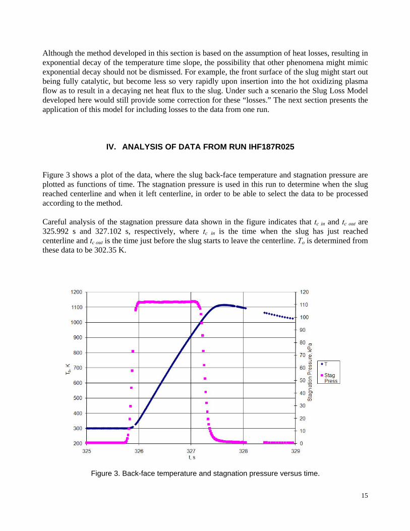
Figure 3 shows a plot of the data, where the slug back-face temperature and stagnation pressure are plotted as functions of time. The stagnation pressure is used in this run to determine when the slug reached centerline and when it left centerline, in order to be able to select the data to be processed according to the method. Careful analysis of the stagnation pressure data shown in the figure indicates that tBc in B and tBc out B are 325.992 s and 327.102 s, respectively, where t Bc in B is the time when the slug has just reached centerline and t Bc outB is the time just before the slug starts to leave the centerline. TBo B is determined from these data to be 302.35 K.
Figure 3. Back-face temperature and stagnation pressure versus time.

16
The physical properties of the copper slug are: Density at 298 K, assumed a constant throughout calculations:
38,925.7 kgm
ρ = (4.1)
Thermal conductivity at 298 K, assumed a constant throughout calculations:
385.2 WkmK
= (4.2)
Heat capacity calculated by the Shomate equation (3.17) at TBoB:
385.615poJc
kgK= (4.3)
Other data for the slug follow:
0.00781D m= (4.4)
0.004529M kg= (4.5)
2 20.25 0.000047906A D mπ= = (4.6)
0.010592ML mAρ
= = (4.7)
Combining equations (2.2) and (2.38), setting cBp B = c BpoB, and substituting for these defined values gives
2
0.99 2
2ln 0.5381 0.99
poR
c Lt s
kρ
π⎛ ⎞= =⎜ ⎟−⎝ ⎠
(4.8)
Add the value of tBR0.99 B to tBc in B to get t B1B = 326.53 s, which defines the lower end of the time span for which the data will be processed. The closest value to this in the data turns out to be t B1 B = 326.532 s. The upper end of the time span, t B2 B, is simply equal to tBc out B = 327.102 s. With t B1B and tB2 B defined, the data to process are shown in table 1. The data-acquisition sampling rate was about 67 data points per second.

17
TABLE 1. BACK-FACE TEMPERATURE VERSUS TIME DATA FROM tB1 B TO tB2 B
Fitting this data to equation (3.7) gives the best linear fit to TBb B versus ( )1b t te− − when b = 0.29160 sP
-1P,
where the RP
2P value of the fit is maximized at 0.99999. The Solver function in an Excel spreadsheet
was used to solve for b. When b is determined, “a” can be calculated according to the equation:
( )( )1intercept 766.76b t tb
Ka T vs e bs
− −= = (4.9)
And TBb1fit B can be calculated according to the equation:
( )( )11 slope 660.32b t t
b fit baT T vs e Kb
− −= + = (4.10)
RBla B can be calculated according to the equation:
1 1.964la
po
KRbMc W
= = (4.11)
And q can be calculated according to equation (3.8):
( )
2 226,005,000 2,6001
6
po o
la
Mc a bT W WqA m cmL
kR A
−= = =
⎛ ⎞−⎜ ⎟
⎝ ⎠
(4.12)
This value is about 15% higher than the value of 2,250 W/cmP
2P reported by the facility test engineers,
where losses were not taken into account.

18
And t Bo B can be calculated according to equation (3.12):
1
1
1 6ln 325.792o
o
b fit
qL aTk bt t sab T
b
⎛ ⎞− −⎜ ⎟= − =⎜ ⎟
⎜ ⎟−⎝ ⎠
(4.13)
The fictitious TBb B(t Bo B) of equation (3.10) can be calculated:
( ) 1836b o oqLT t T K
k= − = (4.14)
The plot in figure 4 shows how the model fits the data. Notice how the fit is extremely good, with error of fit to data of ± 0.07%. Also note that the fit is clearly not linear; this fact is easily seen by holding a straight edge to it. Figure 5 shows a plot of the losses versus time as determined from equations (3.21) and (3.22). Notice how at tB1 B, the earliest point at which the slope would be eligible to be used with the current ASTM method (without corrections for losses), the losses are greater than 10%. And the losses only get larger with time. For comparison, in the test engineer’s report for this run, a heat loss of 345.4 W/cmP
2P was reported
during the cooling phase, after the slug was removed from the flow. Figure 6 shows a plot of the actual loss resistance, RBl B, versus t, calculated according to equa-tion (3.16).
Figure 4. Back-face temperature – fit compared to data.

19
Figure 5. Losses (per cm P
2P slug frontal area) versus time.
0.0
1.0
2.0
3.0
4.0
326.5 326.6 326.7 326.8 326.9 327 327.1 327.2
t, s
Rl,
K/W
Figure 6. Actual loss resistance versus time.

20
V. FINITE ELEMENT ANALYSIS MODEL
A Finite Element Analysis (FEA) model was created using the commercial software program COMSOL Multiphysics, COMSOL, Inc, Burlington, Massachusetts, USA. The slug was modeled using three-dimensional (3-D) tetrahedral elements. Figure 7 shows the mesh. The heat-loss routes from slug to holder for this model were defined as follows (reference to figure 1 is helpful for understanding this description): The actual slug is isolated from its holder by six ruby spheres of 1.5875-mm diameter, three arranged equally spaced around a concentric circle at the back side of the slug, and three arranged equally spaced around the circumference of the slug about midway from front to back. Based on measurements of pronounced dimpling observed on a slug, from the ruby spheres being forced into the copper surface of the slug during use, it was estimated that the area of contact between each ruby sphere and the slug could be represented as a circular area with diameter of 0.6 mm. Therefore, for the FEA model, the surface areas of the slug that make contact with the ruby spheres were modeled as 0.6-mm-diameter surface regions, with a heat-transfer coefficient of h rejecting heat to a temperature of TBo B, the initial temperature of the slug and assumed constant temperature of its holder. These features of the model are shown in figure 8. Note that for the purposes of this model possible heat losses through the air gap between slug and holder via convection and radiation were not considered.
Figure 7. Model mesh.

21
Figure 8. Boundary conditions showing the locations of the entering and exiting heat fluxes
in the model. The slug has the material properties of copper. The heat capacity varies with temperature according to the Shomate equation (3.17). Thermal conductivity (ref. 7) was fit to a linear equation (5.1).
1 2
1 2
2
0.071098
422.915
k c T cWc
m KWc
m K
= +
= −
=
(5.1)
A smoothed Heaviside function (flc2hs from the COMSOL Library) was used to create ramp-up and ramp-down times for the heat flux applied to the front face of the model. The total simulation time of the model is 3 seconds, with a 0.01-second time step. Figure 9 shows a temperature fringe plot at the end of a run (at time t = 3 seconds). Runs were made with the model for various values of qBinputB, h, and duration of heat pulse, until a very close agreement with the actual data was obtained with a value of qBinputB = 2,600 W/cmP
2P. Fig-
ure 10 shows TBbB versus t for both this COMSOL solution and the actual data, where the curves lie almost exactly on top of one another, and figure 11 compares the q values as calculated from the slug calorimeter equation applied to the back face, i.e., per equation (3.18) as applied numerically to the data.

22
Figure 9. Temperature fringe plot of the model at time t = 3 seconds.
Figure 10. TBbB vs. t – COMSOL model and actual data compared.

23
The best fit of the model to the data is obtained with a unique combination of q and h. A sensitivity analysis showed that the values of q and h so determined are known to about ± 1% and ± 10%, respectively. The temperatures of the front and back faces were plotted as a function of time; they are shown in figure 12.
Figure 11. q versus t – COMSOL model and actual data compared.
Figure 12. Temperature vs. time plots for the center of the front and back faces.

24
Alternate COMSOL models were used that were axisymmetric (2-D) where the ruby sphere contacts were modeled as thin concentric rings of contact area. These models gave essentially the same results as the 3-D model already presented, but had the advantage of running much faster. In the data presented in the following discussion, the COMSOL models are all based on the 2-D models, but the results would be expected to be nearly identical if the more time-consuming equivalent 3-D models were run. COMSOL model runs were done for the following four cases: no losses and constant physical properties, no losses and variable physical properties, losses and constant physical properties, and losses and variable physical properties (the 2-D version of the 3-D case already presented). In addition, the ideal partial differential equation solution of equation (2.30) was calculated. These five cases were all based on a qBinputB value of 2,600 W/cmP
2P. Finally, the Slug Loss Model fit of equa-
tion (3.7) was calculated based upon the COMSOL data for the “losses and variable physical properties” case. Figure 13 compares all six of these cases.
Figure 13. Results of all models compared.

25
The ideal partial differential equation solution has a perfect step function, so its initial transient solution is quicker than the “no losses and constant physical properties” COMSOL case that has a smoothed step function, but as expected, these two solutions parallel each other beyond the transient. The “no losses and variable physical properties” case shows more deviation from the ideal case than the “losses and constant physical properties” case, showing that variable heat capacity contributes more to the dropping slope during the heating phase than the losses do. The Slug Loss Model solution fit the “losses and variable physical properties” COMSOL case over the steady-state region, from t = 0.76 s to 1.3 s, the region over which the lengthwise temperature profile is roughly parabolic. As expected, the Slug Loss Model gives a value of TBb B(t BoB) less than TBo B according to equation (3.10), where tBo B calculates to be about 0.04 s according to equation (3.12). When the Slug Loss Model was run on the data from the “losses and variable physical properties” COMSOL case, it gave a q of 2,465 W/cmP
2P, about 5% less than the 2,600 W/cmP
2P value that was
determined from both the Slug Loss Model applied to the actual data and the COMSOL fit to the actual data. The reason for this difference appears to be evident in figure 11. The downward slope of the actual data is steeper over the time interval where the Slug Loss Model was fit than the downward slope of the COMSOL model fit over the same interval. The steeper downward slope is indicative of more losses, which is inferred as a higher q by the Slug Loss Model. Thus, the Slug Loss Model appears to have a bias towards underpredicting q (i.e., not fully correcting for losses) if the data were to have perfectly followed the assumptions of the COMSOL model. Based on this finding, it is best not to apply the Slug Loss Model blindly without also looking at the data plotted in the form of q versus t as in figure 11 to be sure that the data show the basic characteristics upon which the Slug Loss Model is based. Note that in the actual slug calorimeter data case under analysis in this paper, the front face of the slug actually melted at the end of the run. This result did not appear to have a discernable impact on the data. No attempt was made to incorporate this melting in any of the models.
VI. CONCLUSIONS
A mathematical model for determining the heat flux with a slug calorimeter with high heat losses, termed the Slug Loss Model, has been presented. For a particular high-heat-flux arc-jet run, the Slug Loss Model determined a heat flux that is 15% higher than what has been calculated using the conventional approach. It was found to be in good agreement with the FEA model, reinforcing the idea that losses are occurring. This Slug Loss Model is intended to be an additional tool in the thermal analyst’s toolbox that can be applied for high losses.

26
REFERENCES
1. ASTM Standard E457-08: Standard Test Method for Measuring Heat-Transfer Rate Using a
Thermal Capacitance (Slug) Calorimeter. Annual Book of ASTM Standards: Space Simulation; Aerospace and Aircraft; Composite Materials. vol. 15, no. 03, 2008.
2. Diller, T. E.: Advances in Heat Flux Measurements. Advances in Heat Transfer, vol. 23,
Academic Press, 1993, pp. 307–311. 3. Childs, P. R. N.; Greenwood, J. R.; and Long, C. A.: Heat flux measurement techniques. Pro-
ceedings of the Institution of Mechanical Engineers. vol. 213, part C, 1999, pp. 664–665. 4. Powers, D. L.: Boundary Value Problems. 5th ed., Chap. 2. Elsevier Academic Press, New York,
2006. 5. Carslaw, H. S.; and Jaeger, J. C.: Conduction of Heat in Solids. 2nd ed. Oxford University Press,
London, 1959, pp. 112–113. Equation (3). 6. NIST Chemistry WebBook, HThttp://webbook.nist.govTH, data cited as from NIST Standard Refer-
ence Database 69, June 2005. 7. Linde, D. R.: CRC Handbook of Chemistry and Physics. 81st ed., CRC Press, New York, 2000,
p. 12-199.

27

REPORT DOCUMENTATION PAGE
8. PERFORMING ORGANIZATION REPORT NUMBER
10. SPONSORING/MONITOR’S ACRONYM(S)
Form ApprovedOMB No. 0704-0188
13. SUPPLEMENTARY NOTES
7. PERFORMING ORGANIZATION NAME(S) AND ADDRESS(ES)
4. TITLE AND SUBTITLE 5a. CONTRACT NUMBER
6. AUTHOR(S)
1. REPORT DATE (DD-MM-YYYY)
9. SPONSORING/MONITORING AGENCY NAME(S) AND ADDRESS(ES)
2. REPORT TYPE 3. DATES COVERED (From - To)
19a. NAME OF RESPONSIBLE PERSON
19b. TELEPHONE (Include area code)
18. NUMBER OF PAGES
17. LIMITATION OF ABSTRACT
16. SECURITY CLASSIFICATION OF:
15. SUBJECT TERMS
14. ABSTRACT
Standard Form 298 (Rev. 8-98)Prescribed by ANSI Std. Z39-18
The public reporting burden for this collection of information is estimated to average 1 hour per response, including the time for reviewing instructions, searching existingdata sources, gathering and maintaining the data needed, and completing and reviewing the collection of information. Send comments regarding this burden estimate orany other aspect of this collection of information, including suggestions for reducing this burden, to Department of Defense, Washington Headquarters Services,Directorate for information Operations and Reports (0704-0188), 1215 Jefferson Davis Highway, Suite 1204, Arlington, VA 22202-4302. Respondents should be awarethat notwithstanding any other provision of law, no person shall be subject to any penalty for failing to comply with a collection of information if it does not display acurrently valid OMB control number.PLEASE DO NOT RETURN YOUR FORM TO THE ABOVE ADDRESS.
12. DISTRIBUTION/AVAILABILITY STATEMENT
5b. GRANT NUMBER
5c. PROGRAM ELEMENT NUMBER
5d. PROJECT NUMBER
5e. TASK NUMBER
5f. WORK UNIT NUMBER
11. SPONSORING/MONITORING REPORT NUMBER
a. REPORT b. ABSTRACT c. THIS PAGE
Unclassified 34
Unclassified — Unlimited Distribution: NonstandardSubject Category: 34Availability: NASA CASI (301) 621-0390
NASA/TM–2008-215364
09/23/2008
1Thermophysics Facilities Branch, Ames Research Center, Moffett Field, CA 94035-10002Department of Mechanical and Aerospace Engineering, San Jose State University, San Jose, CA 95192
National Aeronautics and Space AdministrationWashington, D. C. 20546-0001
T. Mark Hightower
Thermal Capacitance (Slug) Calorimeter Theory Including HeatLosses and Other Decaying Processes
T. Mark Hightower1, Ricardo A. Olivares1, and Daniel Philippidis2
A mathematical model, termed the Slug Loss Model, has been developed for describing thermal capacitance (slug) calorimeterbehavior when heat losses and other decaying processes are not negligible. This model results in the temperature time slopetaking the mathematical form of exponential decay. When data is found to fit well to this model, it allows a heat flux value to becalculated that corrects for the losses and may be a better estimate of the cold wall fully catalytic heat flux, as is desired in arcjet testing. The model was applied to the data from a copper slug calorimeter inserted during a particularly severe high heatingrate arc jet run to illustrate its use. The Slug Loss Model gave a cold wall heat flux 15% higher than the value of 2,250 W/cm2
obtained from the conventional approach to processing the data (where no correction is made for losses). For comparison, aFinite Element Analysis (FEA) model was created and applied to the same data, where conduction heat losses from the slugwere simulated. The heat flux determined by the FEA model was found to be in close agreement with the heat flux determinedby the Slug Loss Model.
Thermal capacitance calorimeter, Slug calorimeter, Arc jet, Finite element analysis, FEA, COMSOL, Heat losses
Point of Contact: T. Mark Hightower, Ames Research Center, MS 229-4, Moffett Field, CA 94035-1000(650) 604-4443
Technical Memorandum
Unclassified Unclassified
NASA
(650) 604-4443Unclassified
A-080019
WBS 999574.01.02.01.02