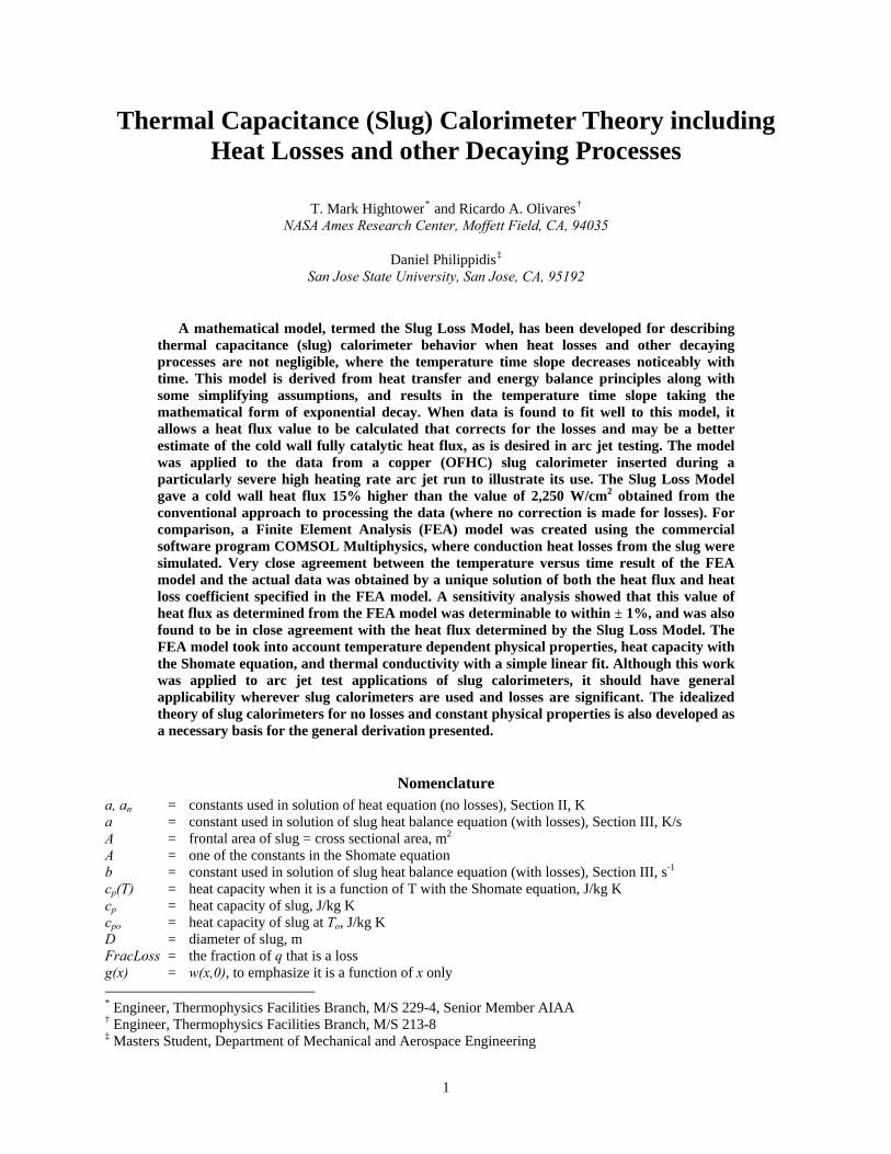
Thermal Capacitance (Slug) Calorimeter Theory including Heat Losses and other Decaying Processes

T. Mark Hightower* and Ricardo A. Olivares† NASA Ames Research Center, Moffett Field, CA, 94035

Daniel Philippidis‡ San Jose State University, San Jose, CA, 95192

A mathematical model, termed the Slug Loss Model, has been developed for describing thermal capacitance (slug) calorimeter behavior when heat losses and other decaying processes are not negligible, where the temperature time slope decreases noticeably with time. This model is derived from heat transfer and energy balance principles along with some simplifying assumptions, and results in the temperature time slope taking the mathematical form of exponential decay. When data is found to fit well to this model, it allows a heat flux value to be calculated that corrects for the losses and may be a better estimate of the cold wall fully catalytic heat flux, as is desired in arc jet testing. The model was applied to the data from a copper (OFHC) slug calorimeter inserted during a particularly severe high heating rate arc jet run to illustrate its use. The Slug Loss Model gave a cold wall heat flux 15% higher than the value of 2,250 W/cm2 obtained from the conventional approach to processing the data (where no correction is made for losses). For comparison, a Finite Element Analysis (FEA) model was created using the commercial software program COMSOL Multiphysics, where conduction heat losses from the slug were simulated. Very close agreement between the temperature versus time result of the FEA model and the actual data was obtained by a unique solution of both the heat flux and heat loss coefficient specified in the FEA model. A sensitivity analysis showed that this value of heat flux as determined from the FEA model was determinable to within ± 1%, and was also found to be in close agreement with the heat flux determined by the Slug Loss Model. The FEA model took into account temperature dependent physical properties, heat capacity with the Shomate equation, and thermal conductivity with a simple linear fit. Although this work was applied to arc jet test applications of slug calorimeters, it should have general applicability wherever slug calorimeters are used and losses are significant. The idealized theory of slug calorimeters for no losses and constant physical properties is also developed as a necessary basis for the general derivation presented.

Nomenclature a, an = constants used in solution of heat equation (no losses), Section II, K a = constant used in solution of slug heat balance equation (with losses), Section III, K/s A = frontal area of slug = cross sectional area, m2 A = one of the constants in the Shomate equation b = constant used in solution of slug heat balance equation (with losses), Section III, s-1 cp(T) = heat capacity when it is a function of T with the Shomate equation, J/kg K cp = heat capacity of slug, J/kg K cpo = heat capacity of slug at To, J/kg K D = diameter of slug, m FracLoss = the fraction of q that is a loss g(x) = w(x,0), to emphasize it is a function of x only * Engineer, Thermophysics Facilities Branch, M/S 229-4, Senior Member AIAA † Engineer, Thermophysics Facilities Branch, M/S 213-8 ‡ Masters Student, Department of Mechanical and Aerospace Engineering

1

h = heat transfer coefficient for surface regions of FEA model, Section V, W/m2 K k = thermal conductivity of slug, W/m K L = length of slug, m M = mass of slug, kg n = series of positive integers, 1,2,3… q = qinput, constant heat flux applied to front face of slug starting at t = 0, W/m2 qindicated = heat flux inferred at back face of slug by equation (2.29), W/m2 qloss = heat flux loss per unit frontal area of slug, W/m2 qslopeTave = heat flux based on the temperature-time slope and heat capacity of Tave, W/m2 qslopeTb = heat flux based on the temperature-time slope and heat capacity of Tb, W/m2 Rl = actual loss resistance, K/W Rla = apparent loss resistance, K/W T(x,t) = temperature of slug as a function of x and t, K T = temperature, K t = time, s to = time when perfect step function “q on” would have occurred, equation (3.12) t1 = time defining lower end of range over which Tb vs t data is fit to equation (3.7) t2 = time defining upper end of range over which Tb vs t data is fit to equation (3.7) tc in = time when the slug has just reached the point of heat flux measurement (i.e. at nozzle centerline for arc jets) tc out = time just preceding when the slug begins to leave the point of heat flux measurement Tave = average temperature of slug, K Tb = back face temperature of slug, K Tb1fit = T of backface corresponding to time t1 according to the best fit of equation (3.7) Tf = front face temperature of slug, K To = uniform T of slug prior to start of application of constant heat flux q at t = 0, K tp = heat penetration time, time for heat to penetrate to back face, s tR = slug response time, s tR0.99 = tR for 0.99 of qinput to be detectible at slug backface, according to equation (2.38), s vss(x,t) = steady state portion of solution to heat equation w(x,t) = transient portion of solution to heat equation x = position along length of slug, x = 0 is front face, x = L is back face, m xc = alternate coordinate for position along length of slug as used in Carslaw & Jaeger text5, where xc = 0 is back face, xc = L is front face, m α = thermal diffusivity of slug, m2/s θ(t) = separation of variables function of t λ = separation of variables constant, m-1 λn = series of separation of variables constants for n = 1,2,3…, m-1 ρ = density of slug, kg/m3 φ(x) = separation of variables function of x, K

I. Introduction A slug calorimeter determines heat flux by measuring the rate at which a slug of material heats up while

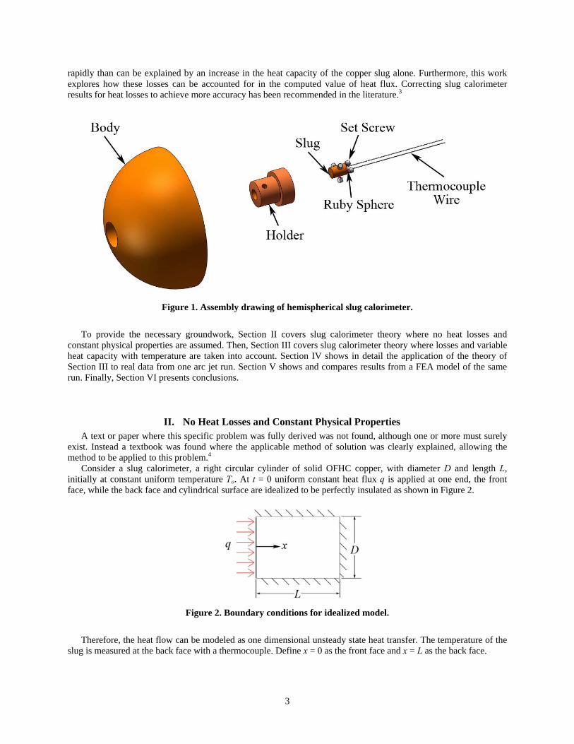
subjected to a heat source. Arc jets are ground test facilities that are used to produce similar heating and flow environments as experienced in planetary atmospheric entry, to test spacecraft thermal protection materials and systems. Slug calorimeters are used for calibration of arc jet test conditions.1 For arc jet applications the slug is usually made of Oxygen-Free High Conductivity (OFHC) copper. An assembly drawing of an arc jet slug calorimeter is shown in Figure 1.

Heat losses from the slug to its holder are an issue, and are hard to control under high heat flux conditions.2 The ASTM standard1 recommends using the slug cool down slope after removal from the heat source as an indication of the losses during the heating phase. This assumes that the conditions causing the losses are the same whether subjected to or removed from the heat source, an assumption that evidence suggests is not always valid. The ASTM standard also recommends that these losses be less than 5% of the heating rate in order to be neglected.

This current work explores how losses during the heating phase can be more directly determined based on the behavior of the temperature time slope during the heating phase, where the temperature time slope decreases more

2

rapidly than can be explained by an increase in the heat capacity of the copper slug alone. Furthermore, this work explores how these losses can be accounted for in the computed value of heat flux. Correcting slug calorimeter results for heat losses to achieve more accuracy has been recommended in the literature.3

Figure 1. Assembly drawing of hemispherical slug calorimeter.

To provide the necessary groundwork, Section II covers slug calorimeter theory where no heat losses and

constant physical properties are assumed. Then, Section III covers slug calorimeter theory where losses and variable heat capacity with temperature are taken into account. Section IV shows in detail the application of the theory of Section III to real data from one arc jet run. Section V shows and compares results from a FEA model of the same run. Finally, Section VI presents conclusions.

II. No Heat Losses and Constant Physical Properties A text or paper where this specific problem was fully derived was not found, although one or more must surely

exist. Instead a textbook was found where the applicable method of solution was clearly explained, allowing the method to be applied to this problem.4

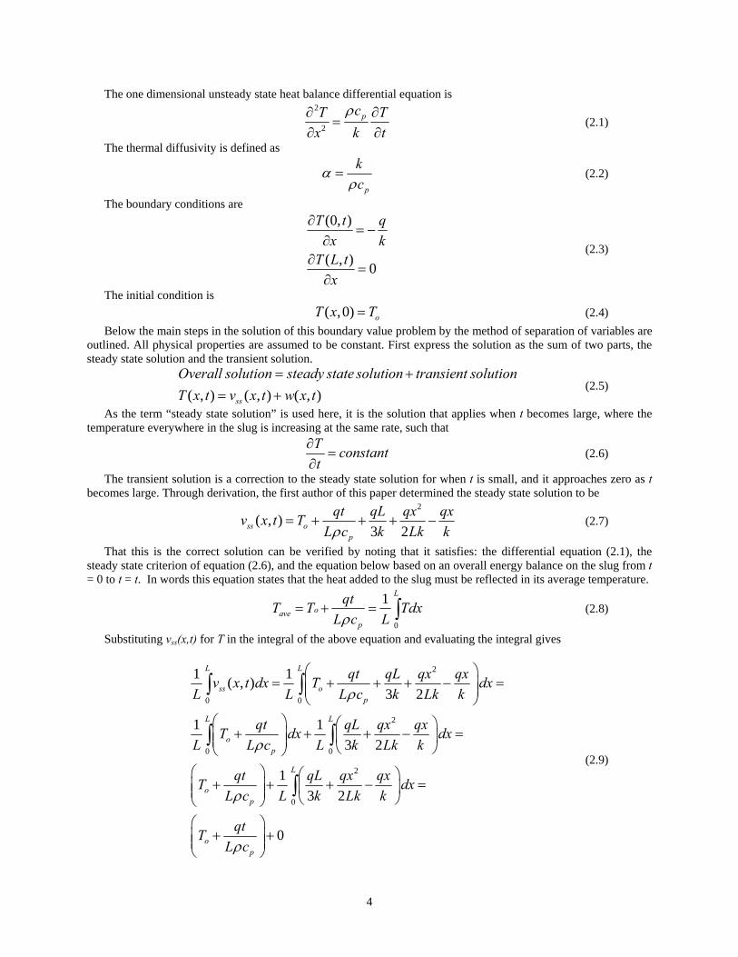
Consider a slug calorimeter, a right circular cylinder of solid OFHC copper, with diameter D and length L, initially at constant uniform temperature To. At t = 0 uniform constant heat flux q is applied at one end, the front face, while the back face and cylindrical surface are idealized to be perfectly insulated as shown in Figure 2.

Figure 2. Boundary conditions for idealized model.

Therefore, the heat flow can be modeled as one dimensional unsteady state heat transfer. The temperature of the

slug is measured at the back face with a thermocouple. Define x = 0 as the front face and x = L as the back face.

3

The one dimensional unsteady state heat balance differential equation is

2

2pcT T

x k tρ∂ ∂

=∂ ∂

(2.1)

The thermal diffusivity is defined as

p

kc

αρ

= (2.2)

The boundary conditions are

(0, )

( , ) 0

T t qx k

T L tx

∂= −

∂∂

=∂

(2.3)

The initial condition is ( ,0) oT x T= (2.4) Below the main steps in the solution of this boundary value problem by the method of separation of variables are

outlined. All physical properties are assumed to be constant. First express the solution as the sum of two parts, the steady state solution and the transient solution.

(2.5) ( , ) ( , ) ( , )ss

Overall solution steady state solution transient solutionT x t v x t w x t

= += +

As the term “steady state solution” is used here, it is the solution that applies when t becomes large, where the temperature everywhere in the slug is increasing at the same rate, such that

T constantt

∂=

∂ (2.6)

The transient solution is a correction to the steady state solution for when t is small, and it approaches zero as t becomes large. Through derivation, the first author of this paper determined the steady state solution to be

2

( , )3 2ss o

p

qt qL qx qxv x t TL c k Lk kρ

= + + + − (2.7)

That this is the correct solution can be verified by noting that it satisfies: the differential equation (2.1), the steady state criterion of equation (2.6), and the equation below based on an overall energy balance on the slug from t = 0 to t = t. In words this equation states that the heat added to the slug must be reflected in its average temperature.

0

1 L

oavep

qtT T TdL c Lρ

= + = x∫ (2.8)

Substituting vss(x,t) for T in the integral of the above equation and evaluating the integral gives

2

0 0

2

0 0

2

0

1 1( , )3 2

1 13 2

13 2

0

L L

ss op

L L

op

L

op

op

qt qL qx qxv x t dx T dxL L L c k Lk k

qt qL qx qxT dx dxL L c L k Lk k

qt qL qx qxT dxL c L k Lk k

qtTL c

ρ

ρ

ρ

ρ

⎛ ⎞= + + + −⎜ ⎟⎜ ⎟

⎝ ⎠⎛ ⎞ ⎛ ⎞

+ + + − =⎜ ⎟ ⎜ ⎟⎜ ⎟ ⎝ ⎠⎝ ⎠⎛ ⎞ ⎛ ⎞

+ + + − =⎜ ⎟ ⎜ ⎟⎜ ⎟ ⎝ ⎠⎝ ⎠⎛ ⎞

+ +⎜ ⎟⎜ ⎟⎝ ⎠

∫ ∫

∫ ∫

∫

=

(2.9)

4

Applying the change of variable from T to w to the differential equation gives

2

2

1w wx tα

∂ ∂=

∂ ∂ (2.10)

The boundary conditions in w are

(0, ) 0

( , ) 0

w tx

w L tx

∂=

∂∂

=∂

(2.11)

The initial condition is

2

( ,0)2 3qx qx qLw xLk k k

−= + − (2.12)

It is the change of variables that allows w to be solved by the separation of variables method, because the boundary conditions in w are homogeneous. So the separation of variables method proposes that

( , ) ( ) ( )w x t x tφ θ= (2.13) Substituting into the partial differential equation produces two ordinary differential equations

2

2

2

2

2

''( ) ( )

( ) '( )

1''( ) ( ) ( ) '( )

''( ) 1 '( )( ) ( )'' 0' 0

w x txw x tt

x t x

x tx t

φ θ

φ θ

φ θ φ θα

φ θ

t

λφ α θφ λ φ

θ αλ θ

∂=

∂∂

=∂

=

= = −

+ =

+ =

(2.14)

The negative sign in front of λ2 is needed, since without it a trivial solution is obtained. The general solutions to

these differential equations are

2

( ) cos sin

( ) t

x a x b

t e αλ

xφ λ λ

θ −

= +

= (2.15)

The boundary conditions become

( , ) '( ) ( )

(0, ) '(0) ( ) 0

( , ) '( ) ( ) 0

w x t x tx

w t tx

w L t L tx

φ θ

φ θ

φ θ

∂=

∂∂

= =∂

∂= =

∂

(2.16)

5

Since ( ) 0tθ = would give a trivial solution, the boundary conditions become

'(0) 0'( ) 0L

φφ

==

(2.17)

Apply the first boundary condition

'(0) 0'( ) sin cos'(0) sin(0) cos(0) 0

0( ) cos

x a x b xa b

bx a x

φφ λ λ λ λφ λ λ

φ λ

== − += − + =

=∴ =

(2.18)

Apply the second boundary condition

'( ) sin 0

1, 2,3...

n

L a LnL

n

φ λ λπλ

= − =

=

=

(2.19)

At this point the solution to the partial differential equation in w can be expressed as

2

1( , ) cos

n tL

nn

n xw x t a eL

παπ ⎛ ⎞∞ − ⎜ ⎟⎝ ⎠

=

⎛ ⎞= ⎜ ⎟⎝ ⎠

∑ (2.20)

Now it remains to apply the initial condition in order to solve for the constants an.

2

1( ,0) cos ( )

2 3nn

n x qx qx qLw x a g xL Lk k kπ∞

=

−⎛ ⎞= = + −⎜ ⎟⎝ ⎠

∑ = (2.21)

This is a problem in Fourier series, which is solved by

2 20

2 2( )cosL

nn x qLa g x dx

L L kπ

π⎛ ⎞= ⎜ ⎟⎝ ⎠∫

1n

= − (2.22)

The transient solution then becomes

2

2 21

2 1( , ) cosn tL

n

qL n xw x t ek n L

παππ

⎛ ⎞∞ − ⎜ ⎟⎝ ⎠

=

⎛ ⎞= − ⎜ ⎟⎝ ⎠

∑ (2.23)

6

Finally, combining equations (2.7) & (2.23), the overall solution to the partial differential equation is

2

2

2 21

2 1( , ) cos3 2

n tL

onp

qt qL qx qx qL n xT x t T eL c k Lk k k n L

παπρ π

⎛ ⎞∞ − ⎜ ⎟⎝ ⎠

=

⎛ ⎞ ⎛ ⎞= + + + − −⎜ ⎟ ⎜ ⎟⎜ ⎟ ⎝ ⎠⎝ ⎠∑ (2.24)

Factoring out common terms and applying equation (2.2) gives

22

2 2 21

1 1 2 1( , ) cos3 2

n tL

on

qL t x x n xT x t T ek L L L n L

παα ππ

⎛ ⎞∞ − ⎜ ⎟⎝ ⎠

=

⎛ ⎞⎛ ⎞ ⎛ ⎞⎜ ⎟= + + + − −⎜ ⎟ ⎜ ⎟⎜ ⎟⎝ ⎠ ⎝ ⎠⎝ ⎠∑ (2.25)

As a check on the above equation, it is worth comparing it to the equivalent solution given in the classic text by

Carslaw and Jaeger.5 What makes comparing the solutions tricky is that their text defines the x coordinate as zero at the back face of the slug and L at the front face. So call the Carslaw and Jaeger text’s coordinate xc to distinguish it from the x of this paper, and make a change of variable in equation (2.25) according to the equation below.

cx L x= − (2.26)

Upon making this change of variable and simplifying, the following equation is obtained, which is exactly

equivalent to that given in the Carslaw and Jaeger text when To is set equal to zero.5

22

2 2 21

1 1 2 ( 1)( , ) cos6 2

nn tLc c

c on

x n xqL tT x t T ek L L n L

παπαπ

⎛ ⎞∞ − ⎜ ⎟⎝ ⎠

=

⎛ ⎞−⎛ ⎞ ⎛ ⎞⎜ ⎟= + − + −⎜ ⎟ ⎜ ⎟⎜ ⎟⎝ ⎠ ⎝ ⎠⎝ ⎠∑ (2.27)

By inspecting equation (2.25), as expected it is seen that as t increases the summation term goes to zero, and the

solution becomes a parabolic temperature profile that is everywhere increasing at the same rate, that

is( , )T x constant

t∂ ∞

=∂

.

( , )

p p

T x q q qAt kL c L Mc

αρ

∂ ∞= = =

∂ (2.28)

where A is the frontal area of the slug and M is its mass. It is this behavior upon which the theory of slug calorimeter operation is based. Once enough time has elapsed,

the rate of change of the back face temperature is the same as the rate of change of temperature everywhere throughout the slug, and therefore the back face temperature captures the incident heat flux q by the following equation.

p bp

Mc dT dTq L cA dt dt

ρ= = b (2.29)

where Tb = the slug back face temperature. The analytical expression for Tb is

2

2 21

1 2 ( 1)( , )6

nn tL

b on

q t qL qLT T L t T ekL k k n

πααπ

⎛ ⎞∞ − ⎜ ⎟⎝ ⎠

=

−= = + − − ∑ (2.30)

7

The analytical expression for the front face temperature Tf is

2

2 21

1 2 1(0, )3

n tL

f on

q t qL qLT T t T ekL k k n

πααπ

⎛ ⎞∞ − ⎜ ⎟⎝ ⎠

=

= = + + − ∑ (2.31)

The average temperature of the slug Tave is given by

0

1( )L

ave ave oq tT T t T TdkL Lα

= = + = x∫ (2.32)

The following difference equations can be written

2

2

(2 1)

2 21

2 21

1 4 12 (2 1)

1 2 ( 1)6

n tL

f bn

nn tL

ave bn

qL qLT T ek k n

qL qLT T ek k n

πα

πα

π

π

−⎛ ⎞∞ − ⎜ ⎟⎝ ⎠

=

⎛ ⎞∞ − ⎜ ⎟⎝ ⎠

=

− = −−

−− = +

∑

∑ (2.33)

The summations in all of the above equations approach zero as t becomes large. It can be shown that if enough time has elapsed for the heat to have just penetrated to the backside of the slug,

the summation terms above are well represented by truncating the summations with the first term, for t greater than or equal to the penetration time tp.

2

2

1 26

tL

b oq t qL qLT T ekL k k

πααπ

⎛ ⎞− ⎜ ⎟⎝ ⎠= + − + (2.34)

Take the derivative and set equal to zero to solve for tp.

2

2

2

2 0

ln(2)

ptLb

p

dT q q edt kL kL

Lt

παα α

απ

⎛ ⎞− ⎜ ⎟⎝ ⎠= − =

=

(2.35)

Now do a more general treatment, for response time, tR. Make a distinction between qinput to the front face and

qindicated based on the slug calorimeter equation applied at the back face.

2 2

21 2

R

input

bindicated p

bp t tp p L Lindicated

input input

q q

dTq L cdtdTL c c cq dt e e

q q k k

π πα α

ρ

ρ ρ α ρ α ⎛ ⎞ ⎛ ⎞− −⎜ ⎟ ⎜ ⎟⎝ ⎠ ⎝ ⎠

=

=

⎛ ⎞⎜ ⎟⎝ ⎠= = − = −

(2.36)

8

2

2

2ln1

Rindicated

input

Lt qq

απ

⎛ ⎞⎜ ⎟⎜=⎜ ⎟−⎜ ⎟⎝ ⎠

⎟ (2.37)

For practical purposes, the response time calculated when 0.99indicated

input

qq

= should be sufficient elapsed time for

the heat flux determination from the back face temperature to begin to be valid.

2

0.99 2

2ln1 0.99R

Ltαπ

⎛ ⎞= ⎜ −⎝ ⎠⎟ (2.38)

In the next section, this value tR0.99 will be used as the response time necessary to ensure that the slug has reached steady state, where the temperature profile has established its parabolic shape.

III. Heat Losses and Variable Heat Capacity – Slug Loss Model In this section the theory is developed to handle the case of slug calorimeters where heat losses from slug to

surroundings (as well as other possible decaying processes) are taken into account. This is done for the purpose of creating a model to fit to real data, where losses are often evident by a T versus t slope that decreases with time more than can be accounted for by the increasing heat capacity of the copper slug with temperature alone.

A heat balance on the slug with losses gives

( )( . . )

ave o avepo

la

input output i e losses accumulationT T dTqA Mc

R dt

− =

−− =

(3.1)

The surroundings (slug holder) to which the slug loses heat is assumed to be at the same temperature as the

initial temperature of the slug, To, and this surrounding temperature is assumed to remain constant. Rla is defined as the apparent resistance to heat loss, which is coupled with cpo, the constant value of cp at temperature To. This is done so that the above equation can be analytically integrated. Later the actual resistance to heat loss, Rl, will be solved for when heat capacity as a function of temperature, cp(Tave), is introduced. At this point the effect of increasing cp with temperature is taken into account as an additional apparent loss incorporated into the value of Rla.

It is desired to get the above equation in terms of Tb, the temperature that is recorded as data. Assume that enough time has elapsed so that the parabolic temperature profile through the slug has been established, which should be the case for t > tR0.99 from equation (2.38). From equation (2.33) for t > tR0.99, the summation drops out as zero and gives

6ave bqLT T

k− = (3.2)

Solving this equation for Tave gives

6ave bqLT T

k= + (3.3)

Substituting this into equation (3.1) gives

6

o b

po la po la po la po

T TA Lq bdTMc kR Mc R Mc R Mc dt

⎛ ⎞⎛ ⎞− + −⎜ ⎟⎜ ⎟⎜ ⎟⎜ ⎟⎝ ⎠⎝ ⎠

= (3.4)

9

Defining two constants

6

1

o

po la po la po

la po

TA La qMc kR Mc R Mc

bR Mc

⎛ ⎞⎛ ⎞= − +⎜ ⎟⎜ ⎟⎜ ⎟⎜ ⎟⎝ ⎠⎝

=

⎠ (3.5)

Equation (3.4) can be written as

bb

dTa bTdt

− = (3.6)

This equation integrates to

( )11

b t tb b fit

a aT T eb b

− −⎛ ⎞= − +⎜ ⎟⎝ ⎠

(3.7)

This equation can be used to fit actual slug calorimeter data recorded during an arc jet run by taking the

following steps. First determine the time when the slug arrived at the position where the heat flux is to be measured. Then add

tR0.99 from equation (2.38) to this time to get t1, the initial time for which the data will be processed. This ensures that steady state has been reached by time t1. Next, determine t2, the final time for which the data will be processed, by taking the time just before the slug begins to be removed from the heat source. Now there is a range of Tb versus t data points from t1 to t2 to fit with equation (3.7). (If the slug has been left exposed to the heat source longer than is necessary, an alternate approach might also be used to select t2. In such a case, adding tR0.99 or perhaps 1.5 times tR0.99 to t1 to get t2 might be a better approach. This would help ensure the validity of the assumption of constant surrounding temperature To up to the value of t2 where the model is being applied.)

Next assume a value of “b” and plot Tb versus ( )1b t te− − , which should be linear according to the equation. Next determine the value of “b” that gives the best linear fit. This can be done by solving for “b” that maximizes the R2 value (coefficient of determination) for the fit. Now that “b” is known, “a” can be solved for from the intercept of the fit. Finally, Tb1fit can be solved for from the slope of the fit. The model equation fit to the data is now complete and ready to be compared to the data.

Once the data has been processed and “a” and “b” have been determined, q can be solved for by solving equation (3.5) for q.

( )

166

po oo

lapo la po

Mc a bTa bTqA LA L

kR AMc kR Mc

−−= =⎛ ⎞ ⎛

−−⎜ ⎟ ⎜⎜ ⎟ ⎝ ⎠⎝ ⎠

⎞⎟

(3.8)

An alternate but equivalent equation for q is

6

poo

Mc qLq a b TA k

⎛ ⎞⎛ ⎞= − −⎜ ⎟⎜ ⎟⎝ ⎠⎝ ⎠

(3.9)

Take equation (3.7) and go back in time to to, the theoretical time when the step function of “q on” would have

occurred had it been a perfect step function. This is going back in time while keeping the temperature profile of the slug at steady-state. This is an idealization that differs from the actual behavior, but whether idealized or actual, the energy that heats up the slug from to to t1 is the same. At t = to, Tave = To. According to equation (3.2)

( )6b o oqLT t T

k= − (3.10)

10

When going back in time while maintaining a steady state parabolic temperature profile, the temperature at the back face at to has to be less than To so that Tave = To. Substituting equation (3.10) into equation (3.7) gives

( )11( )

6ob t t

b o o b fitqL a aT t T T e

k b− −⎛ ⎞= − = − +⎜ ⎟

⎝ ⎠ b (3.11)

Solving this equation for to gives

1

1

1 6lno

o

b fit

qL aTk bt t ab T

b

⎛ ⎞− −⎜ ⎟= − ⎜

⎜ ⎟−⎝ ⎠

⎟ (3.12)

Equation (3.7) gives Tb as an analytical function of time, which can be written as Tb(t) to make the t functionality

explicit. By using the linear relationship between Tave and Tb of equation (3.3) Tave can now also be expressed as an analytical function of time, Tave(t).

( )11( )

6b t t

ave b fita aT t T eb b

− −⎛ ⎞⎛ ⎞= − + +⎜ ⎟⎜⎝ ⎠⎝ ⎠

qLk⎟ (3.13)

The derivative of Tave(t) with respect to time can also be taken analytically

( 11

( ) b t taveb fit

dT t ab T edt b

)− −⎛ ⎞= − −⎜ ⎟⎝ ⎠

(3.14)

We are now in a position to introduce cp as a function of Tave into the differential equation (3.1) as well as the

actual loss resistance, Rl.

( )( ) ( )( ( ))ave o ave

p avel

T t T dT tqA Mc T tR dt−

− = (3.15)

This equation can now be solved for Rl as a function of time

( )( )

( )( )( ( ))

ave ol

avep ave

T t TR t

dT tqA Mc T tdt

−=⎛ ⎞−⎜ ⎟⎝ ⎠

(3.16)

It remains to express cp for copper as a function of Tave by the Shomate equation.

2 32

22

4 73 4

6

( )

2.789933 10 4.421789 10

4.918152 10 2.19879 10

1.079706 10

p ave ave ave aveave

Ec T A BT CT DTT

whereJ JA x B x

kgK kgKJ JC x D x

kgK kgKJKE xkg

−

− −

= + + + +

= =

= − =

=

1 (3.17)

11

The Shomate equation can be found at the NIST web site.6 The equation given by NIST was modified to get the temperature units as shown above, and to get it on a mass basis rather than a mole basis, by applying the conversion of the atomic weight for copper, 63.546 g/gmole.

So now all the elements that allow the calculation of Rl(t) by equation (3.16) have been assembled. Other useful equations can also be written. Two equations can be written for heat flux based on the temperature-

time slope and heat capacity, one based on Tb and the other based on Tave.

( ( )) ( )( ) p b b

slopeTb

Mc T t dT tq tA dt

= (3.18)

( ( )) ( )( ) p ave ave

slopeTave

Mc T t dT tq tA dt

= (3.19)

Equation (3.18) is essentially equivalent to the current ASTM method where no correction for losses is attempted

if time is chosen to be early in the steady state region, i.e. t = t1. Equation (3.19) is similar, but is probably slightly more accurate, being based on Tave rather than Tb. Keep in mind that in the above equations where temperatures and derivatives of temperatures are explicitly expressed as functions of time, these functions of time all stem from the model’s fit to the data, equation (3.7).

By comparing equation (3.19) to equation (3.9), noting equations (3.10) & (3.6), recognizing that the time derivatives of Tave and Tb are equal by inspection of equation (3.3), and that ( )ave o oT t T= , it can be shown that

( )

( ( )) ( )6

( ) ( )

slopeTave o

po p ave o ave oo

opo pob ave o

q q t

Mc Mc T t dT tqLa b TA k A

Mc McdT t dT tA dt A dt

=

⎛ ⎞⎛ ⎞− − =⎜ ⎟⎜ ⎟⎝ ⎠⎝ ⎠

⎛ ⎞ =⎜ ⎟⎝ ⎠

dt (3.20)

Finally, the following equations can be written for heat flux loss and fraction loss as functions of time.

( ( )) ( )( ) ( ) p ave ave

loss slopeTave

Mc T t dT tq t q q t qA dt

= − = − (3.21)

( ( )) ( )( ) 1 p ave aveMc T t dT tFracLoss tqA dt

= − (3.22)

Although the method developed in this section is based on the assumption of heat losses, resulting in exponential

decay of the temperature time slope, the possibility that other phenomena might mimic exponential decay should not be dismissed. For example, the front surface of the slug might start out being fully catalytic, but become less so very rapidly upon insertion into the hot oxidizing plasma flow so as to result in a decaying net heat flux to the slug. Under such a scenario the Slug Loss Model developed here would still provide some correction for these “losses.” The next section presents the application of this model for including losses, to the data from one run.

12

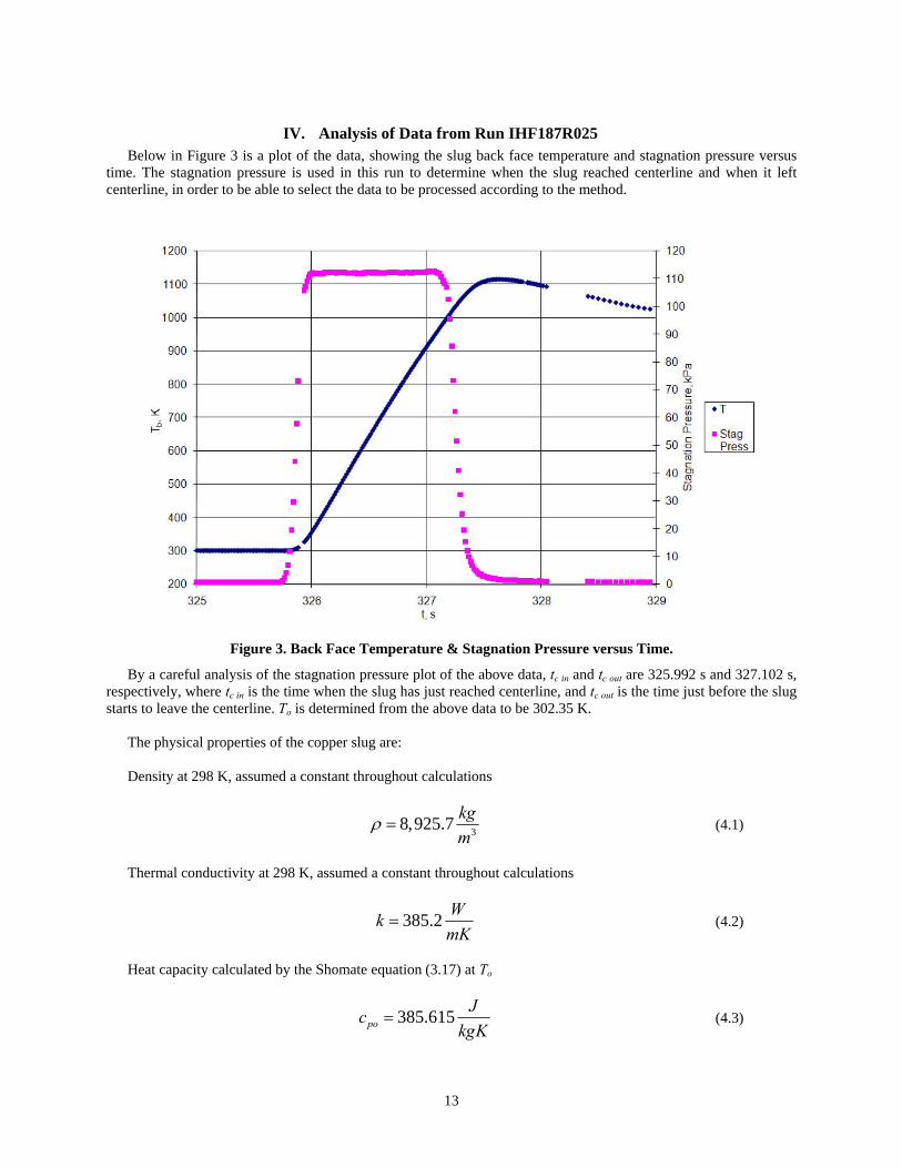
IV. Analysis of Data from Run IHF187R025 Below in Figure 3 is a plot of the data, showing the slug back face temperature and stagnation pressure versus

time. The stagnation pressure is used in this run to determine when the slug reached centerline and when it left centerline, in order to be able to select the data to be processed according to the method.

Figure 3. Back Face Temperature & Stagnation Pressure versus Time.

By a careful analysis of the stagnation pressure plot of the above data, tc in and tc out are 325.992 s and 327.102 s, respectively, where tc in is the time when the slug has just reached centerline, and tc out is the time just before the slug starts to leave the centerline. To is determined from the above data to be 302.35 K.

The physical properties of the copper slug are: Density at 298 K, assumed a constant throughout calculations

38,925.7 kgm

ρ = (4.1)

Thermal conductivity at 298 K, assumed a constant throughout calculations

385.2 WkmK

= (4.2)

Heat capacity calculated by the Shomate equation (3.17) at To

385.615poJc

kgK= (4.3)

13

Other data for the slug is as follows: 0.00781D m= (4.4) 0.004529M kg= (4.5)

(4.6) 20.25 0.000047906A Dπ= = 2m

0.010592MLAρ

= = m (4.7)

Combining equations (2.2) and (2.38), setting cp = cpo, and substituting for the above defined values gives

2

0.99 2

2ln 0.5381 0.99

poR

c Lt

kρπ

⎛ ⎞= ⎜ ⎟−⎝ ⎠s= (4.8)

Add the value of tR0.99 to tc in to get t1 = 326.53 s, which defines the lower end of the time span for which the data

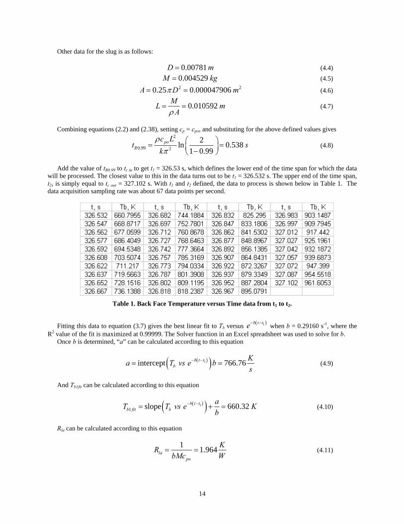
will be processed. The closest value to this in the data turns out to be t1 = 326.532 s. The upper end of the time span, t2, is simply equal to tc out = 327.102 s. With t1 and t2 defined, the data to process is shown below in Table 1. The data acquisition sampling rate was about 67 data points per second.

Table 1. Back Face Temperature versus Time data from t1 to t2.

Fitting this data to equation (3.7) gives the best linear fit to Tb versus ( )1b t te− − when b = 0.29160 s-1, where the

R2 value of the fit is maximized at 0.99999. The Solver function in an Excel spreadsheet was used to solve for b. Once b is determined, “a” can be calculated according to this equation

( )( )1intercept 766.76b t tb

Ka T vs e bs

− −= = (4.9)

And Tb1fit can be calculated according to this equation

( )( )11 slope 660.32b t t

b fit baT T vs eb

− −= + = K (4.10)

Rla can be calculated according to this equation

1 1.964la

po

KRbMc W

= = (4.11)

14

And q can be calculated according to equation (3.8)

( )

226,005,000 2,6001

6

po o

la

Mc a bT W WqA mL

kR A

−= = =

⎛ ⎞−⎜ ⎟

⎝ ⎠

2cm (4.12)

This value is about 15% higher than the value of 2,250 W/cm2 reported by the facility test engineers, where

losses were not taken into account. And to can be calculated according to equation (3.12)

1

1

1 6ln 325.792o

o

b fit

qL aTk bt t ab T

b

⎛ ⎞− −⎜ ⎟= − =⎜ ⎟

⎜ ⎟−⎝ ⎠

s (4.13)

The fictitious Tb(to) of equation (3.10) can be calculated.

( ) 1836b o oqLT t T K

k= − = (4.14)

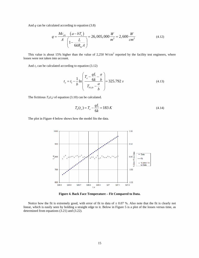
The plot in Figure 4 below shows how the model fits the data.

Figure 4. Back Face Temperature – Fit Compared to Data.

Notice how the fit is extremely good, with error of fit to data of ± 0.07 %. Also note that the fit is clearly not

linear, which is easily seen by holding a straight edge to it. Below in Figure 5 is a plot of the losses versus time, as determined from equations (3.21) and (3.22).

15

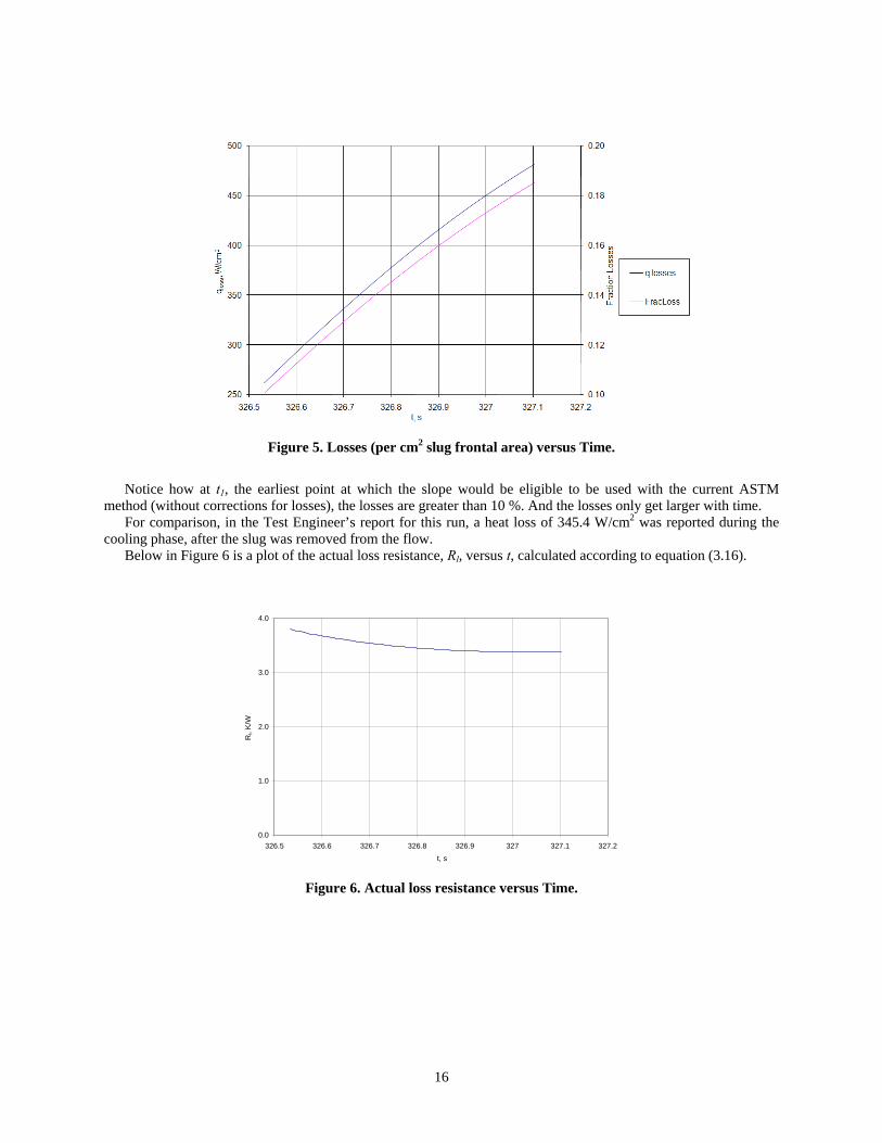
Figure 5. Losses (per cm2 slug frontal area) versus Time.

Notice how at t1, the earliest point at which the slope would be eligible to be used with the current ASTM

method (without corrections for losses), the losses are greater than 10 %. And the losses only get larger with time. For comparison, in the Test Engineer’s report for this run, a heat loss of 345.4 W/cm2 was reported during the

cooling phase, after the slug was removed from the flow. Below in Figure 6 is a plot of the actual loss resistance, Rl, versus t, calculated according to equation (3.16).

0.0

1.0

2.0

3.0

4.0

326.5 326.6 326.7 326.8 326.9 327 327.1 327.2

t, s

Rl,

K/W

Figure 6. Actual loss resistance versus Time.

16

V. Finite Element Analysis Model A simple Finite Element Analysis (FEA) model was created using the commercial software program COMSOL

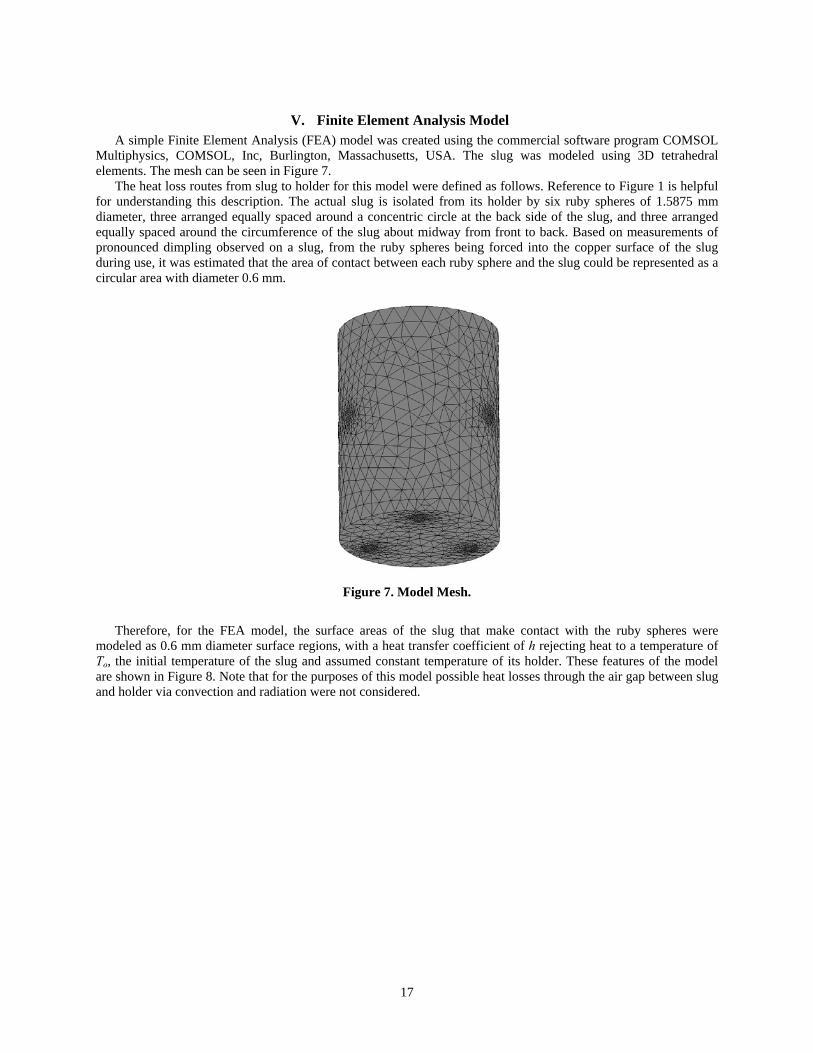
Multiphysics, COMSOL, Inc, Burlington, Massachusetts, USA. The slug was modeled using 3D tetrahedral elements. The mesh can be seen in Figure 7.

The heat loss routes from slug to holder for this model were defined as follows. Reference to Figure 1 is helpful for understanding this description. The actual slug is isolated from its holder by six ruby spheres of 1.5875 mm diameter, three arranged equally spaced around a concentric circle at the back side of the slug, and three arranged equally spaced around the circumference of the slug about midway from front to back. Based on measurements of pronounced dimpling observed on a slug, from the ruby spheres being forced into the copper surface of the slug during use, it was estimated that the area of contact between each ruby sphere and the slug could be represented as a circular area with diameter 0.6 mm.

Figure 7. Model Mesh.

Therefore, for the FEA model, the surface areas of the slug that make contact with the ruby spheres were

modeled as 0.6 mm diameter surface regions, with a heat transfer coefficient of h rejecting heat to a temperature of To, the initial temperature of the slug and assumed constant temperature of its holder. These features of the model are shown in Figure 8. Note that for the purposes of this model possible heat losses through the air gap between slug and holder via convection and radiation were not considered.

17

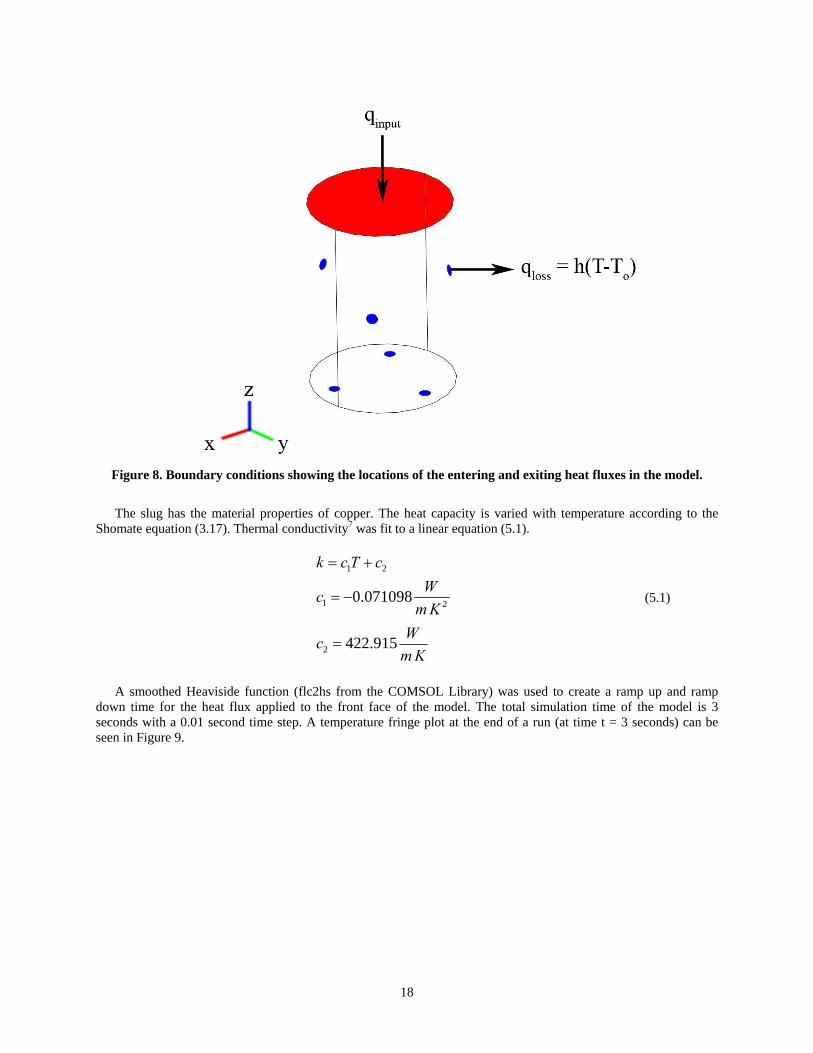
Figure 8. Boundary conditions showing the locations of the entering and exiting heat fluxes in the model.

The slug has the material properties of copper. The heat capacity is varied with temperature according to the

Shomate equation (3.17). Thermal conductivity7 was fit to a linear equation (5.1).

1 2

1 2

2

0.071098

422.915

k c T cWc

m KWc

m K

= +

= −

=

(5.1)

A smoothed Heaviside function (flc2hs from the COMSOL Library) was used to create a ramp up and ramp

down time for the heat flux applied to the front face of the model. The total simulation time of the model is 3 seconds with a 0.01 second time step. A temperature fringe plot at the end of a run (at time t = 3 seconds) can be seen in Figure 9.

18

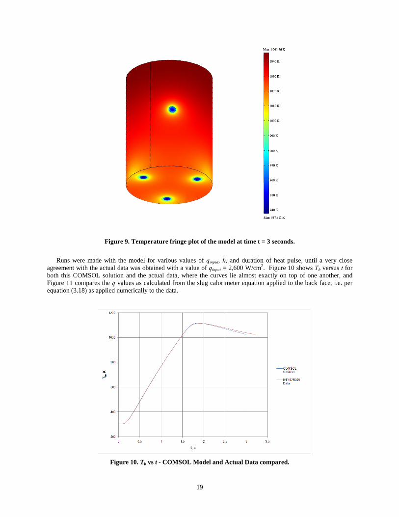
Figure 9. Temperature fringe plot of the model at time t = 3 seconds.

Runs were made with the model for various values of qinput, h, and duration of heat pulse, until a very close

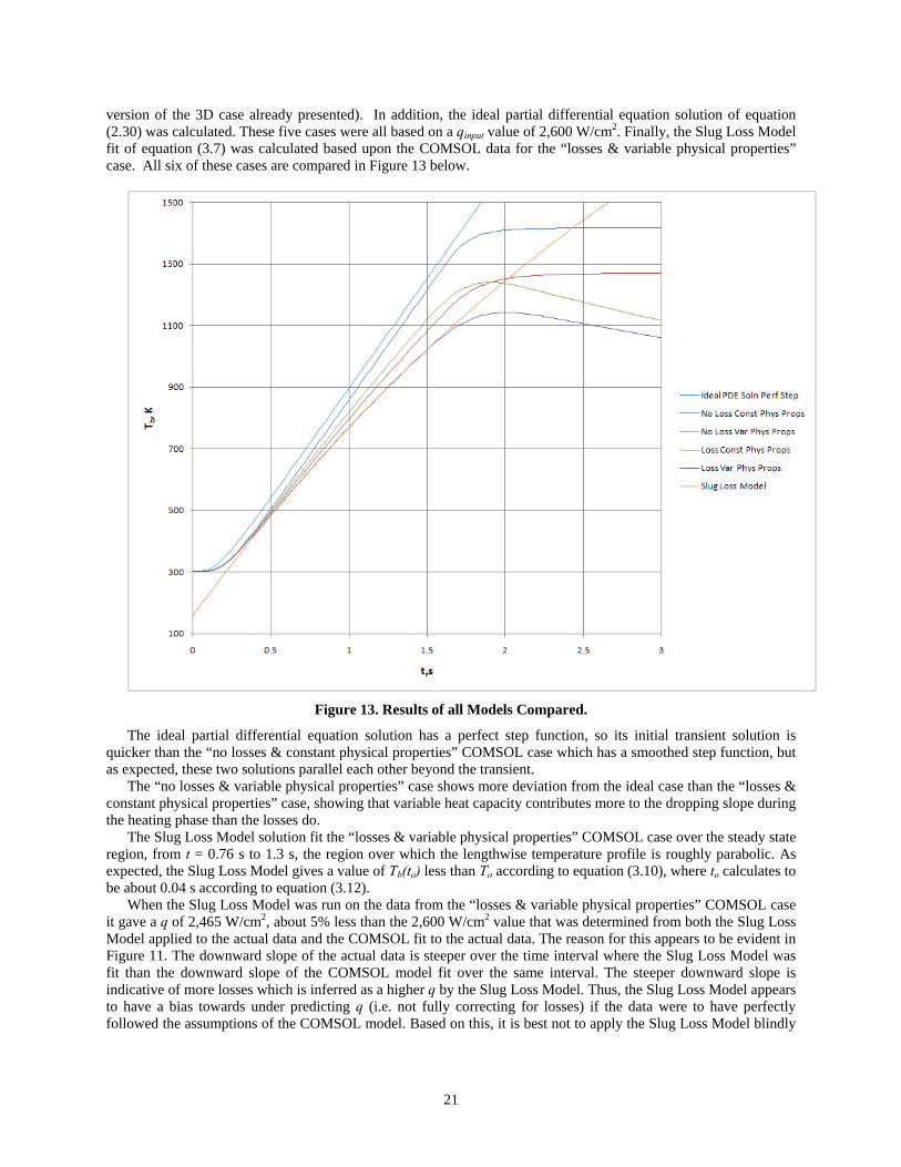
agreement with the actual data was obtained with a value of qinput = 2,600 W/cm2. Figure 10 shows Tb versus t for both this COMSOL solution and the actual data, where the curves lie almost exactly on top of one another, and Figure 11 compares the q values as calculated from the slug calorimeter equation applied to the back face, i.e. per equation (3.18) as applied numerically to the data.

Figure 10. Tb vs t - COMSOL Model and Actual Data compared.

19

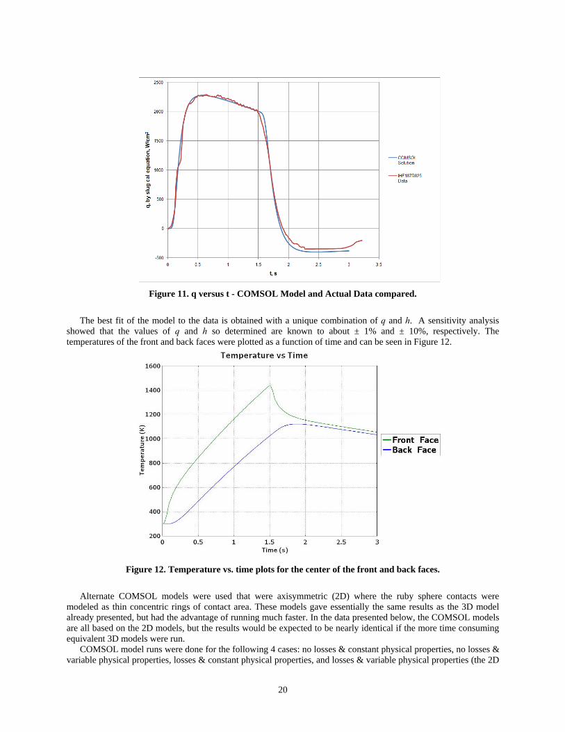
Figure 11. q versus t - COMSOL Model and Actual Data compared.

The best fit of the model to the data is obtained with a unique combination of q and h. A sensitivity analysis

showed that the values of q and h so determined are known to about ± 1% and ± 10%, respectively. The temperatures of the front and back faces were plotted as a function of time and can be seen in Figure 12.

Figure 12. Temperature vs. time plots for the center of the front and back faces.

Alternate COMSOL models were used that were axisymmetric (2D) where the ruby sphere contacts were

modeled as thin concentric rings of contact area. These models gave essentially the same results as the 3D model already presented, but had the advantage of running much faster. In the data presented below, the COMSOL models are all based on the 2D models, but the results would be expected to be nearly identical if the more time consuming equivalent 3D models were run.

COMSOL model runs were done for the following 4 cases: no losses & constant physical properties, no losses & variable physical properties, losses & constant physical properties, and losses & variable physical properties (the 2D

20

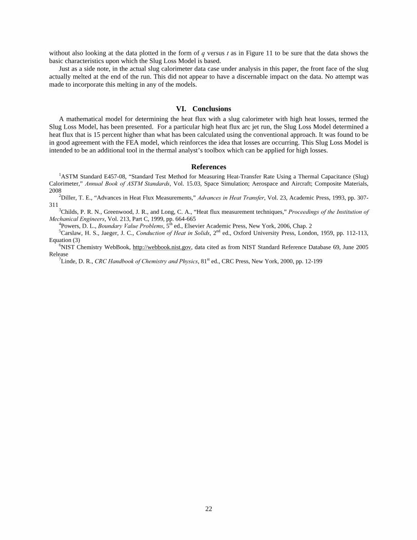
version of the 3D case already presented). In addition, the ideal partial differential equation solution of equation (2.30) was calculated. These five cases were all based on a qinput value of 2,600 W/cm2. Finally, the Slug Loss Model fit of equation (3.7) was calculated based upon the COMSOL data for the “losses & variable physical properties” case. All six of these cases are compared in Figure 13 below.

Figure 13. Results of all Models Compared.

The ideal partial differential equation solution has a perfect step function, so its initial transient solution is quicker than the “no losses & constant physical properties” COMSOL case which has a smoothed step function, but as expected, these two solutions parallel each other beyond the transient.

The “no losses & variable physical properties” case shows more deviation from the ideal case than the “losses & constant physical properties” case, showing that variable heat capacity contributes more to the dropping slope during the heating phase than the losses do.

The Slug Loss Model solution fit the “losses & variable physical properties” COMSOL case over the steady state region, from t = 0.76 s to 1.3 s, the region over which the lengthwise temperature profile is roughly parabolic. As expected, the Slug Loss Model gives a value of Tb(to) less than To according to equation (3.10), where to calculates to be about 0.04 s according to equation (3.12).

When the Slug Loss Model was run on the data from the “losses & variable physical properties” COMSOL case it gave a q of 2,465 W/cm2, about 5% less than the 2,600 W/cm2 value that was determined from both the Slug Loss Model applied to the actual data and the COMSOL fit to the actual data. The reason for this appears to be evident in Figure 11. The downward slope of the actual data is steeper over the time interval where the Slug Loss Model was fit than the downward slope of the COMSOL model fit over the same interval. The steeper downward slope is indicative of more losses which is inferred as a higher q by the Slug Loss Model. Thus, the Slug Loss Model appears to have a bias towards under predicting q (i.e. not fully correcting for losses) if the data were to have perfectly followed the assumptions of the COMSOL model. Based on this, it is best not to apply the Slug Loss Model blindly

21

22

without also looking at the data plotted in the form of q versus t as in Figure 11 to be sure that the data shows the basic characteristics upon which the Slug Loss Model is based.

Just as a side note, in the actual slug calorimeter data case under analysis in this paper, the front face of the slug actually melted at the end of the run. This did not appear to have a discernable impact on the data. No attempt was made to incorporate this melting in any of the models.

VI. Conclusions A mathematical model for determining the heat flux with a slug calorimeter with high heat losses, termed the

Slug Loss Model, has been presented. For a particular high heat flux arc jet run, the Slug Loss Model determined a heat flux that is 15 percent higher than what has been calculated using the conventional approach. It was found to be in good agreement with the FEA model, which reinforces the idea that losses are occurring. This Slug Loss Model is intended to be an additional tool in the thermal analyst’s toolbox which can be applied for high losses.

References 1ASTM Standard E457-08, “Standard Test Method for Measuring Heat-Transfer Rate Using a Thermal Capacitance (Slug)

Calorimeter,” Annual Book of ASTM Standards, Vol. 15.03, Space Simulation; Aerospace and Aircraft; Composite Materials, 2008

2Diller, T. E., “Advances in Heat Flux Measurements,” Advances in Heat Transfer, Vol. 23, Academic Press, 1993, pp. 307-311

3Childs, P. R. N., Greenwood, J. R., and Long, C. A., “Heat flux measurement techniques,” Proceedings of the Institution of Mechanical Engineers, Vol. 213, Part C, 1999, pp. 664-665

4Powers, D. L., Boundary Value Problems, 5th ed., Elsevier Academic Press, New York, 2006, Chap. 2 5Carslaw, H. S., Jaeger, J. C., Conduction of Heat in Solids, 2nd ed., Oxford University Press, London, 1959, pp. 112-113,

Equation (3) 6NIST Chemistry WebBook, http://webbook.nist.gov, data cited as from NIST Standard Reference Database 69, June 2005

Release 7Linde, D. R., CRC Handbook of Chemistry and Physics, 81st ed., CRC Press, New York, 2000, pp. 12-199