Embed Size (px)
Citation preview

Contents i
The Theory and Practice ofConcurrency
A.W. Roscoe
Published 1997, revised to 2000 and lightly revised to 2005.
The original version is in print in April 2005 with Prentice-Hall (Pearson).This version is made available for personal reference only. This version is
copyright ( c©) Pearson and Bill Roscoe.


Contents
Preface ix
0 Introduction 1
0.1 Background 1
0.2 Perspective 4
0.3 Tools 7
0.4 What is a communication? 8
I A FOUNDATION COURSE IN CSP 11
1 Fundamental concepts 13
1.1 Fundamental operators 14
1.2 Algebra 29
1.3 The traces model and traces refinement 35
1.4 Tools 48
2 Parallel operators 51
2.1 Synchronous parallel 51
2.2 Alphabetized parallel 55
2.3 Interleaving 65
2.4 Generalized parallel 68

iv Contents
2.5 Parallel composition as conjunction 70
2.6 Tools 74
2.7 Postscript: On alphabets 76
3 Hiding and renaming 77
3.1 Hiding 77
3.2 Renaming and alphabet transformations 86
3.3 A basic guide to failures and divergences 93
3.4 Tools 99
4 Piping and enslavement 101
4.1 Piping 101
4.2 Enslavement 107
4.3 Tools 112
5 Buffers and communication 115
5.1 Pipes and buffers 115
5.2 Buffer tolerance 127
5.3 The alternating bit protocol 130
5.4 Tools 136
5.5 Notes (2005) 137
6 Termination and sequential composition 139
6.1 What is termination? 139
6.2 Distributed termination 143
6.3 Laws 144
6.4 Effects on the traces model 147
6.5 Effects on the failures/divergences model 148
II THEORY 151
7 Operational semantics 153
7.1 A survey of semantic approaches to CSP 153
7.2 Transition systems and state machines 155

Contents v
7.3 Firing rules for CSP 162
7.4 Relationships with abstract models 174
7.5 Tools 181
7.6 Notes 182
8 Denotational semantics 183
8.1 Introduction 183
8.2 The traces model 186
8.3 The failures/divergences model 195
8.4 The stable failures model 211
8.5 Notes 218
9 Analyzing the denotational models 221
9.1 Deterministic processes 221
9.2 Analyzing fixed points 227
9.3 Full abstraction 232
9.4 Relations with operational semantics 242
9.5 Notes 247
10 Infinite traces 249
10.1 Calculating infinite traces 249
10.2 Adding failures 255
10.3 Using infinite traces 262
10.4 Notes 271
11 Algebraic semantics 273
11.1 Introduction 273
11.2 Operational semantics via algebra 275
11.3 The laws of ⊥N 279
11.4 Normalizing 281
11.5 Sequential composition and SKIP 291
11.6 Other models 294
11.7 Notes 297

vi Contents
12 Abstraction 299
12.1 Modes of abstraction 30012.2 Reducing specifications 31012.3 Abstracting errors: specifying fault tolerance 31312.4 Independence and security 32012.5 Tools 33012.6 Notes 330
III PRACTICE 335
13 Deadlock! 337
13.1 Basic principles and tree networks 33713.2 Specific ways to avoid deadlock 34913.3 Variants 36513.4 Network decomposition 37613.5 The limitations of local analysis 37913.6 Deadlock and tools 38113.7 Notes 386
14 Modelling discrete time 389
14.1 Introduction 38914.2 Meeting timing constraints 39014.3 Case study 1: level crossing gate 39514.4 Checking untimed properties of timed processes 40514.5 Case study 2: the alternating bit protocol 41014.6 Urgency and priority 41714.7 Tools 42014.8 Notes 420
15 Case studies 423
15.1 Combinatorial systems: rules and tactics 42415.2 Analysis of a distributed algorithm 43015.3 Distributed data and data-independence 44515.4 Analyzing crypto-protocols 46815.5 Notes 488

Contents vii
A Mathematical background 491
A.1 Partial orders 491
A.2 Metric spaces 510
B A guide to machine-readable CSP 519
B.1 Introduction 519
B.2 Expressions 520
B.3 Pattern matching 526
B.4 Types 528
B.5 Processes 532
B.6 Special definitions 535
B.7 Mechanics 538
B.8 Missing features 539
B.9 Availability 539
C The operation of FDR 541
C.1 Basic operation 541
C.2 Hierarchical compression 553
Notation 563
Bibliography 567
Main index 577
Index of named processes 589


Preface
Since C.A.R. Hoare’s text Communicating Sequential Processes was published in1985, his notation has been extensively used for teaching and applying concurrencytheory. This book is intended to provide a comprehensive text on CSP from theperspective that 12 more years of research and experience have brought.
By far the most significant development in this time has been the emer-gence of tools to support both the teaching and industrial application of CSP. Thishas turned CSP from a notation used mainly for describing ‘toy’ examples whichcould be understood and analyzed by hand, into one which can and does supportthe description of industrial-sized problems and which facilitates their automatedanalysis. As we will see, the FDR model checking tool can, over a wide range ofapplication areas, perform analyses and solve problems that are beyond most, if notall, humans.
In order to use these tools effectively you need a good grasp of the fundamen-tal concepts of CSP: the tools are most certainly not an alternative to gaining anunderstanding of the theory. Therefore this book is still, in the first instance, a texton the principles of the language rather than being a manual on how to apply itstools. Nevertheless the existence of the tools has heavily influenced both the choiceand presentation of material. Most of the chapters have a section specifically on theway the material in them relates to tools, two of the appendices are tool-related,and there is an associated web site
http://www.comlab.ox.ac.uk/oucl/publications/books/concurrency/
on which readers can find
• a list of tools available for CSP

x Preface
• demonstrations and details of some of the tools
• directories of example files containing most of the examples from the textand many other related ones
• practical exercises which can be used by those teaching and learning fromthis book
• a list of materials available to support teaching (overhead foils, solutions toexercises, etc.) and instructions for obtaining them
as well as supporting textual material. Contact information, etc., relating to thosetools specifically mentioned in the text can be found in the Bibliography.
The Introduction (Chapter 0) gives an indication of the history, purpose andrange of applications of CSP, as well as a brief survey of the classes of tools thatare available. There is also a discussion of how to go about one of the major stepswhen using CSP to model a system: deciding what constitutes an event. It providesbackground reading which should be of interest to more experienced readers beforebeginning the rest of the book; those with no previous exposure to concurrencymight find some parts of the Introduction of more benefit after looking at Part I.
The rest of the book is divided into three parts and structured to make itusable by as wide an audience as possible. It should be emphasized, however, thatthe quantity of material and the differing levels of sophistication required by varioustopics mean that I expect it will be relatively uncommon for people to attempt thewhole book in a short space of time.
Part I (Chapters 1–6) is a foundation course on CSP, covering essentiallythe same ground as Hoare’s text except that most of the mathematical theory isomitted. At an intuitive level, it introduces the ideas behind the operational (i.e.,transition system), denotational (traces, failures and divergences) and algebraicmodels of CSP, but the formal development of these is delayed to Part II. PartI has its origins in a set of notes that I developed for an introductory 16-lecturecourse for Oxford undergraduates in Engineering and Computing Science. I wouldexpect that all introductory courses would cover up to Section 5.1 (buffers), with thethree topics beyond that (buffer tolerance, communications protocols and sequentialcomposition1) being more optional.
Part II and Part III (Chapters 7–12 and 13–15, though Chapter 12 arguablybelongs equally to both) respectively go into more detail on the theory and practice
1Instructors who are intending to deal at any length with the theory presented in Part II shouldconsider carefully whether they want to include the treatment of sequential composition, since itcan reasonably be argued that the special cases it creates are disproportionate to the usefulness ofthat operator in the language. Certainly it is well worth considering presenting the theory withoutthese extra complications before going back to see how termination and sequencing fit in.

Preface xi
of CSP. Either of them would form the basis of a one-term graduate course as afollow-on to Part I, though some instructors will doubtless wish to mix the materialand to include extracts from Parts II and III in a first course. (At Oxford, intro-ductory courses for more mathematically sophisticated audiences have used partsof Chapters 8 and 9, on the denotational semantics and its applications, and somecourses have used part of Chapter 13, on deadlock.) The chapters of Part III arelargely independent of each other and of Part II.2
This book assumes no mathematical knowledge except for a basic under-standing of sets, sequences and functions. I have endeavoured to keep the level ofmathematical sophistication of Parts I and III to the minimum consistent with giv-ing a proper explanation of the material. While Part II does not require any furtherbasic knowledge other than what is contained in Appendix A (which gives an intro-duction to the ideas from the theory of partial orders and metric/restriction spacesrequired to understand the denotational models), the mathematical constructionsand arguments used are sometimes significantly harder than in the other two parts.
Part II describes various approaches to the semantic analysis of CSP. De-pending on your point of view, you can either regard its chapters as an introductionto semantic techniques for concurrency via the medium of CSP, or as a compre-hensive treatment of the theory of this language. Each of the three complementarysemantic approaches used – operational, denotational and algebraic – is directlyrelevant to an understanding of how the automated tools work. My aim in this parthas been to give a sufficiently detailed presentation of the underlying mathematicsand of the proofs of the main results to enable the reader to gain a thorough under-standing of the semantics. Necessarily, though, the most complex and technicalproofs are omitted.
Chapter 12 deserves a special mention, since it does not so much introducesemantic theory as apply it. It deals with the subject of abstraction: forminga view of what a process looks like to a user who can only see a subset of itsalphabet. A full understanding of the methods used requires some knowledge ofthe denotational models described in Chapters 8, 9 and 10 (which accounts for theplacing of Chapter 12 in Part II). However, their applications (to the formulationof specifications in general, and to the specification of fault tolerance and securityin particular), are important and deserve attention by the ‘practice’ community aswell as theoreticians.
Chapter 13, on deadlock avoidance, is included because deadlock is a much
2The only dependency is of Section 15.2 on Chapter 14. It follows from this idependence thata course based primarily on Part III need not cover the material in order and that instructors canexercise considerable freedom in selecting what to teach. For example, the author has taught atool-based graduate course based on Section 15.1, Chapter 5, Section 15.2, Appendix C, Chapter14, Chapter 12 (Sections 12.3 and 12.4 in particular), the first half of Chapter 13 and Section 15.4.

xii Preface
feared phenomenon and there is an impressive range of techniques, both analytic andautomated, for avoiding it. Chapter 14 describes how the untimed version of CSP(the one this book is about) can be used to describe and reason about timed systemsby introducing a special event to represent the passage of time at regular intervals.This has become perhaps the most used dialect of CSP in industrial applications ofFDR. Each of these two chapters contains extensive illustrative examples; Chapter15 is based entirely around five case studies (two of which are related) chosen toshow how CSP can successfully model, and FDR can solve, interesting, difficultproblems from other application areas.
The first appendix, as described above, is an introduction to mathematicaltopics used in Part II. The second gives a brief description of the machine-readableversion of CSP and the functional programming language it contains for manipulat-ing process state. The third explains the operation of FDR in terms of the theoryof CSP, and in particular describes the process-compression functions it uses.
At the end of each chapter in Parts II and III there is a section entitled‘Notes’. These endeavour, necessarily briefly, to put the material of the chapter incontext and to give appropriate references to related work.
Exercises are included throughout the book. Those in Part I are mainlydesigned to test the reader’s understanding of the preceding material; many ofthem have been used in class at Oxford over the past three years. Some of thosein Parts II and III have the additional purpose of developing sidelines of the theorynot otherwise covered.
Except for one important change (the decision not to use process alphabets,see page 76), I have endeavoured to remain faithful to the notation and ideas pre-sented in Hoare’s text. There are a few other places, particularly in my treatmentof termination, variable usage and unbounded nondeterminism, where I have eithertidied up or extended the language and/or its interpretation.
Bill RoscoeMay 1997
Acknowledgements
I had the good fortune to become Tony Hoare’s research student in 1978, which gaveme the opportunity to work with him on the development of the ‘process algebra’version of CSP and its semantics from the first. I have constantly been impressedthat the decisions he took in structuring the language have stood so well the twintests of time and practical use in circumstances he could not have foreseen. Thework in this book all results, either directly or indirectly, from his vision. Those

Preface xiii
familiar with his book will recognize that much of my presentation, and many ofmy examples, have been influenced by it.
Much of the theory set out in Chapters 7, 8, 9 and 11 was established by theearly 1980s. The two people most responsible, together with Tony and myself, forthe development of this basic theoretical framework for CSP were Steve Brookesand Ernst-Rudiger Olderog, and I am delighted to acknowledge their contributions.We were, naturally, much influenced by the work of those such as Robin Milner,Matthew Hennessy and Rocco de Nicola who were working at the same time onother process algebras.
Over the years, both CSP and my understanding of it have benefited from thework of too many people for me to list their individual contributions. I would like tothank the following present and former students, colleagues, collaborators and corre-spondents for their help and inspiration: Samson Abramsky, Phil Armstrong, GeoffBarrett, Stephen Blamey, Philippa Hopcroft (nee Broadfoot), Sadie Creese, NaiemDathi, Jim Davies, Richard Forster, Paul Gardiner, Michael Goldsmith, AnthonyHall, Jifeng He, Huang Jian, Jason Hulance, David Jackson, Lalita JategaonkarJagadeesan, Alan Jeffrey, Mark Josephs, Ranko Lazic, Eldar Kleiner, Gavin Lowe,Helen McCarthy, Jeremy Martin, Albert Meyer, Michael Mislove, Nick Moffat, LeeMomtahan, Tom Newcomb, David Nowak, Joel Ouaknine, Ata Parashkevov, DavidPark, Sriram Rajamani, Joy Reed, Mike Reed, Jakob Rehof, Bill Rounds, PeterRyan, Jeff Sanders, Bryan Scattergood, Steve Schneider, Brian Scott, Karen Seidel,Jane Sinclair, Antti Valmari, David Walker, Wang Xu, Jim Woodcock, Ben Worrell,Zhenzhong Wu, Lars Wulf, Jay Yantchev, Irfan Zakiuddin and Zhou Chao Chen.Many of them will recognize specific influences their work has had on my book. Afew of these contributions are referred to in individual chapters.
I would also like thank all those who told me about errors and typos in theoriginal edition.
Special thanks are due to the present and former staff of Formal Systems(some of whom are listed above) for their work in developing FDR, and latterlyProBE. The remarkable capabilities of FDR transformed my view of CSP and mademe realize that writing this book had become essential. Bryan Scattergood waschiefly responsible for both the design and the implementation of the ASCII versionof CSP used on these and other tools. I am grateful to him for writing Appendix Bon this version of the language. The passage of years since 1997 has only emphasisedthe amazing job he did in designing CSPM , and the huge expressive power of theembedded functional language. Ranko Lazic has both provided most of the resultson data independence (see Section 15.3.2), and did (in 2000) most of the work inpresenting it in this edition.
Many of the people mentioned above have read through drafts of my bookand pointed out errors and obscurities, as have various students. The quality of

xiv Preface
the text has been greatly helped by this. I have had valuable assistance from JimDavies in my use of LATEX.
My work on CSP has benefited from funding from several bodies over theyears, including EPSRC, DRA, ESPRIT, industry and the US Office of Naval Re-search. I am particularly grateful to Ralph Wachter from the last of these, withoutwhom most of the research on CSP tools would not have happened, and who hasspecifically supported this book and the associated web site.
This book could never have been written without the support of my wifeCoby. She read through hundreds of pages of text on a topic entirely foreign toher, expertly pointing out errors in spelling and style. More importantly, she putup with me writing it.
Internet edition
The version here was extensively updated by me in 2000, with the addition of somenew material (in particular a new section for Chapter 15). Various errors have alsobeen corrected, but please continue to inform me of any more.
A great deal more interesting work has been done on CSP since 1997 thanthis version of the book reports. Much of that appears, or is referenced, in paperswhich can be downloaded from my web site or from those of other current andformer members of the Oxford Concurrency group such as Gavin Lowe, ChristieBolton and Ranko Lazic. As I write this I anticipate the imminent publication (inLNCS) of the proceedings of the BCS FACS meeting in July last year on “25 yearsof CSP”. This will provide an excellent snapshot of much recent work on CSP. Ihave given a brief description of some of this extra work in paragraphs marked 2005,mainly in the notes sections at the ends of chapters. These contain a few citationsbut do not attempt to cover the whole literature of interest.
If anyone reading this has any feedback on any sort of book – either followingon from (part of) this one or something completely different – that you would liketo see written on CSP, please let me know.
Bill RoscoeApril 2005

Chapter 0
Introduction
CSP is a notation for describing concurrent systems (i.e., ones where there is morethan one process existing at a time) whose component processes interact with eachother by communication. Simultaneously, CSP is a collection of mathematical mod-els and reasoning methods which help us understand and use this notation. In thischapter we discuss the reasons for needing a calculus like CSP and some of thehistorical background to its development.
0.1 Background
Parallel computers are starting to become common, thanks to developing technol-ogy and our seemingly insatiable demands for computing power. They provide themost obvious examples of concurrent systems, which can be characterized as sys-tems where there are a number of different activities being carried out at the sametime. But there are others: at one extreme we have loosely coupled networks ofworkstations, perhaps sharing some common file-server; and at the other we havesingle VLSI circuits, which are built from many subcomponents which will often dothings concurrently. What all examples have in common is a number of separatecomponents which need to communicate with each other. The theory of concur-rency is about the study of such communicating systems and applies equally to allthese examples and more. Though the motivation and most of the examples we seeare drawn from areas related to computers and VLSI, other examples can be foundin many fields.
CSP was designed to be a notation and theory for describing and analyzingsystems whose primary interest arises from the ways in which different compo-nents interact at the level of communication. To understand this point, considerthe design of what most programmers would probably think of first when paral-

2 Introduction
lelism is mentioned, namely parallel supercomputers and the programs that run onthem. These computers are usually designed (though the details vary widely) sothat parallel programming is as easy as possible, often by enforcing highly stylizedcommunication which takes place in time to a global clock that also keeps the var-ious parallel processing threads in step with each other. Though the design of theparallel programs that run on these machines – structuring computations so thatcalculations may be done in parallel and so that transfers of information requiredfit the model provided by the computer – is an extremely important subject, it isnot what CSP or this book is about. For what is interesting there is understandingthe structure of the problem or algorithm, not the concurrent behaviour (the clockand regimented communication having removed almost all interest here).
In short, we are developing a notation and calculus to help us understandinteraction. Typically the interactions will be between the components of a concur-rent system, but sometimes they will be between a computer and external humanusers. The primary applications will be areas where the main interest lies in thestructure and consequences of interactions. These include aspects of VLSI design,communications protocols, real-time control systems, scheduling, computer security,fault tolerance, database and cache consistency, and telecommunications systems.Case studies from most of these can be found in this book: see the table of contents.
Concurrent systems are more difficult to understand than sequential ones forvarious reasons. Perhaps the most obvious is that, whereas a sequential program isonly ‘at’ one line at a time, in a concurrent system all the different components are in(more or less) independent states. It is necessary to understand which combinationsof states can arise and the consequences of each. This same observation meansthat there simply are more states to worry about in parallel code, because thetotal number of states grows exponentially (with the number of components) ratherthan linearly (in the length of code) as in sequential code. Aside from this stateexplosion there are a number of more specific misbehaviours which all create theirown difficulties and which any theory for analyzing concurrent systems must be ableto model.
Nondeterminism
A system exhibits nondeterminism if two different copies of it may behave differentlywhen given exactly the same inputs. Parallel systems often behave in this waybecause of contention for communication: if there are three subprocesses P ,Q andR where P and Q are competing to be the first to communicate with R, which inturn bases its future behaviour upon which wins the race, then the whole systemmay veer one way or the other in a manner that is uncontrollable and unobservablefrom the outside.
Nondeterministic systems are in principle untestable, since however many

0.1 Background 3
times one of them behaves correctly in development with a given set of data, itis impossible to be sure that it will still do so in the field (probably in subtlydifferent conditions which might influence the way a nondeterministic decision istaken). Only by formal understanding and reasoning can one hope to establishany property of such a system. One property we might be able to prove of a givenprocess is that it is deterministic (i.e., will always behave the same way when offereda given sequence of communications), and thus amenable to testing.
Deadlock
A concurrent system is deadlocked if no component can make any progress, generallybecause each is waiting for communication with others. The most famous exampleof a deadlocked system is the ‘five dining philosophers’, where the five philosophersare seated at a round table with a single fork between each pair (there is a pictureof them on page 61). But each philosopher requires both neighbouring forks to eat,so if, as in the picture, all get hungry simultaneously and pick up their left-handfork then they deadlock and starve to death. Even though this example is anthro-pomorphic, it actually captures one of the major causes of real deadlocks, namelycompetition for resources. There are numerous others, however, and deadlock (par-ticularly nondeterministic deadlock) remains one of the most common and fearedills in parallel systems.
Livelock
All programmers are familiar with programs that go into infinite loops, never tointeract with their environments again. In addition to the usual causes of this typeof behaviour – properly called divergence, where a program performs an infiniteunbroken sequence of internal actions – parallel systems can livelock. This occurswhen a network communicates infinitely internally without any component com-municating externally. As far as the user is concerned, a livelocked system lookssimilar to a deadlocked one, though perhaps worse since the user may be able toobserve the presence of internal activity and so hope eternally that some outputwill emerge eventually. Operationally and, as it turns out, theoretically, the twophenomena are very different.
The above begin to show why it is essential to have both a good under-standing of the way concurrent systems behave and practical methods for analyzingthem. On encountering a language like CSP for the first time, many people askwhy they have to study a new body of theory, and new specification/verificationtechniques, rather than just learning another programming language. The reasonis that, unfortunately, mathematical models and software engineering techniquesdeveloped for sequential systems are usually inadequate for modelling the subtletiesof concurrency so we have to develop these things alongside the language.

4 Introduction
0.2 Perspective
As we indicated above, a system is said to exhibit concurrency when there can beseveral processes or subtasks making progress at the same time. These subtasksmight be running on separate processors, or might be time-sharing on a singleone. The crucial thing which makes concurrent systems different from sequentialones is the fact that their subprocesses communicate with each other. So while asequential program can be thought of as progressing through its code a line at atime – usually with no external influences on its control-flow – in a concurrent systemeach component is at its own line, and without relying on a precise knowledge of theimplementation we cannot know what sequence of states the system will go through.Since the different components are influencing each other, the complexities of thepossible interactions are mind-boggling. The history of concurrency consists bothof the construction of languages and concepts to make this complexity manageable,and the development of theories for describing and reasoning about interactingprocesses.
CSP has its origins in the mid 1970s, a time when the main practical problemsdriving work on concurrency arose out of areas such as multi-tasking and operatingsystem design. The main problems in those areas are ones of maintaining an illusionof simultaneous execution in an environment where there are scarce resources. Thenature of these systems frequently makes them ideally suited to the model of aconcurrent system where all processes are able (at least potentially) to see thewhole of memory, and where access to scarce resources (such as a peripheral) iscontrolled by semaphores. (A process seeks a semaphore by executing a claim, orP , operation, and after its need is over releases it with a V operation. The systemmust enforce the property that only one process ‘has’ the semaphore at a time. Thisis one solution to the so-called mutual exclusion problem.)
Perhaps the most superficially attractive feature of shared-variable concur-rency is that it is hardly necessary to change a programming language to accom-modate it. A piece of code writes to, or reads from, a shared variable in very muchthe same way as it would do with a private one. The concurrency is thus, fromthe point of view of a sequential program component, in some senses implicit. Aswith many things, the shared variable model of concurrency has its advantages anddisadvantages. The main disadvantage from the point of view of modelling gen-eral interacting systems is that the communications between components, whichare plainly vitally important, happen too implicitly. This effect also shows up whenit comes to mathematical reasoning about system behaviour: when it is not madeexplicit in a program’s semantics when it receives communications, one has to allowfor the effects of any communication at any time.
In recent years, of course, the emphasis on parallel programming has moved

0.2 Perspective 5
to the situation where one is distributing a single task over a number of separateprocessors. If done wrongly, the communications between these can represent a realbottleneck, and certainly an unrestricted shared variable model can cause problemsin this way. One of the most interesting developments to overcome this has beenthe BSP (Bulk Synchronous Parallelism) model [76, 130] in which the processorsare synchronized by the beat of a relatively infrequent drum and where the commu-nication/processing trade-off is carefully managed. The BSP model is appropriatefor large parallel computations of numerical problems and similar; it does not giveany insight into the way parallel systems interact at a low level. When you needthis, a model in which the communications between processors are the essence ofprocess behaviour is required. If you were developing a parallel system on which torun BSP programs, you could benefit from using a communication-based model atseveral different levels.
In his 1978 paper [54], C.A.R. Hoare introduced, with the language CSP(Communicating Sequential Processes), the concept of a system of processes, eachwith its own private set of variables, interacting only by sending messages to eachother via handshaken communication. That language was, at least in appearance,very different from the one studied in this book. In many respects it was like thelanguage occam [57, 60] which was later to evolve from CSP, but it differed fromoccam in one or two significant ways:
• Parallelism was only allowed into the program at the highest syntactic level.Thus the name Communicating Sequential Processes was appropriate in afar more literal way than with subsequent versions of CSP.
• One process communicated with another by name, as if there were a singlechannel from each process to every other. In occam, processes communicateby named channels, so that a given pair might have none or many betweenthem.
The first version of CSP was the starting point for a large proportion of thework on concurrency that has gone on since. Many researchers have continued touse it in its original form, and others have built upon its ideas to develop their ownlanguages and notations.
The great majority of these languages have been notations for describing andreasoning about purely communicating systems: the computations internal to thecomponent processes’ state (variables, assignments, etc.) being forgotten about.They have come to be known as process algebras. The first of these were Milner’sCCS [80, 82] and Hoare’s second version of CSP, the one this book is about. Itis somewhat confusing that both of Hoare’s notations have the same name andacronym, since in all but the deepest sense they have little in common. Henceforth,

6 Introduction
for us, CSP will mean the second notation. Process algebra notations and theoriesof concurrency are useful because they bring the problems of concurrency into sharpfocus. Using them it is possible to address the problems that arise, both at the highlevel of constructing theories of concurrency, and at the lower level of specifying anddesigning individual systems, without worrying about other issues. The purpose ofthis book is to describe the CSP notation and to help the reader to understand itand, especially, to use it in practical circumstances.
The design of process algebras and the building of theories around them hasproved an immensely popular field over the past two decades. Concurrency provesto be an intellectually fascinating subject and there are many subtle distinctionswhich one can make, both at the level of choice of language constructs and in thesubtleties of the theories used to model them. From a practical point of view theresulting tower of Babel has been unfortunate, since it has both created confusionand meant that perhaps less effort than ought to have been the case has beendevoted to the practical use of these methods. It has obscured the fact that oftenthe differences between the approaches were, to an outsider, insignificant.
Much of this work has, of course, strongly influenced the development ofCSP and the theories which underlie it. This applies both to the untimed versionof CSP, where one deliberately abstracts from the precise times when events occur,and to Timed CSP, where these times are recorded and used. Untimed theories tendto have the advantages of relative simplicity and abstraction, and are appropriatefor many real circumstances. Indeed, the handshaken communication of CSP is tosome extent a way of making precise timing of less concern, since, if one end of thecommunication is ready before the other, it will wait. Probably for these reasonsthe study of untimed theories generally preceded that of the timed ones. The timedones are needed because, as we will see later on, one sometimes needs to rely upontiming details for the correctness of a system. This might either be at the level ofoverall (externally visible) behaviour, or for some internal reason. The realizationof this, and the increasing maturity of the untimed theories, have led to a growingnumber of people working on real-time theories since the mid 1980s.
There are a number of reasons why it can be advantageous to combine timedand untimed reasoning. The major ones are listed below.
• Since timed reasoning is more detailed and complex than untimed, it is usefulto be able to localize timed analysis to the parts of the system which reallydepend on it.
• In many cases proving a timed specification can be factored into proving acomplex untimed one and a simple timed property. This is attractive for thesame reasons as above.

0.3 Tools 7
• We might well want to develop a system meeting an untimed specificationbefore refining it to meet detailed timing constraints.
There have been two distinct approaches to introducing time into CSP, andfortunately the above advantages are available in both. The first, usually known asTimed CSP (see, for example, [29, 31, 98, 99]), uses a continuous model of time andhas a mathematical theory quite distinct to the untimed version. To do it justicewould require more space than could reasonably be made available in this volume,and therefore we do not cover it. A complementary text by S.A. Schneider, basedprimarily round Timed CSP, is in preparation at the time of writing.
The continuous model of time, while elegant, makes the construction of auto-mated tools very much harder. It was primarily for this reason that the authorproposes (in Chapter 14) an alternative in which a timed interpretation is placedon the ‘untimed’ language. This represents the passage of time by the regularoccurrence of a specific event (tock) and had the immediate advantage that theuntimed tools were applicable. While less profound than Timed CSP, it does, forthe time being at least, seem more practical. It has been used frequently in industrialapplications of FDR.
0.3 Tools
For a long time CSP was an algebra that was reasoned about only manually. Thiscertainly had a strong influence on the sort of examples people worked on – thelack of automated assistance led to a concentration on small, elegant examples thatdemonstrated theoretical niceties rather than practical problems.
In the last few years there has been an explosion of interest in the develop-ment of automated proof tools for CSP and similar languages. The chief proof andanalytic tool for CSP at present is called FDR (standing for Failures/DivergencesRefinement, a name which will be explained in Section 3.3), whose existence hasled to a revolution in the way CSP is used. To a lesser extent it has also influencedthe way CSP is modelled mathematically and the presentation of its models.
A number of other tools, with similar external functionality though based onvery different algorithms, have been or are being developed. FDR appears to be themost powerful (for most purposes) and complete at the time of writing. Becauseof this, and because the author has played a leading role in its development andis therefore more familiar with it than other tools, this book is, so far as the useof tools is concerned, centred chiefly on FDR. Many of the examples and exerciseshave been designed so they can be ‘run’ on it.
Equally useful from the point of view of learning about the language aresimulators and animators which allow the human user to experiment with CSP

8 Introduction
processes: interacting with them in reality instead of having to imagine doing so.The difference between this sort of tool and FDR is that simulations do not proveresults about processes, merely providing a form of implementation that allowsexperimentation. At the time of writing the most capable such tool appears to beProBE (used by the author in a preliminary version and due to be released later in1997).
The above are general-purpose tools, in that they deal with more-or-less anyprogram and desired property which you want to investigate. More specific tools arecustomized to perform analyses of restricted classes of system (such as protocols)or to check for specific conditions such as deadlock.
These and other tool developments have led to a restructuring and standard-ization of the CSP notation itself. The fact that the tools have allowed so manymore practical-size examples to be developed has certainly influenced our percep-tion of the relative importance and, too, uses of various parts of the language,especially the parts which are at the level of describing data and operations over it(for building individual communications, and constructing a process’s state). Thepresentation in this book has been influenced by this experience and is based onthe standardized syntax with the important difference that (at the time of writing)the machine-readable syntax is ASCII, and the textual appearance of various con-structs therefore differs from the more elegantly typeset versions which appear herein print. The ASCII syntax is given in an appendix and is used in Chapter 15 (CaseStudies).
On past experience it is reasonable to expect that the range and power oftools will increase markedly over the next few years. Thus a snap-shot from mid1997 would soon get out of date. It is hoped to keep the web site associated withthis book (see Preface) as up-to-date as possible on developments and to includeappropriate references and demonstrations there.
It is only really since the advent of tools that CSP has been used to a sig-nificant extent for the development and analysis of practical and industrial-scaleexamples.
0.4 What is a communication?
CSP is a calculus for studying processes which interact with each other and theirenvironment by means of communication. The most fundamental object in CSP istherefore a communication event. These events are assumed to be drawn from aset Σ (the Greek capital letter ‘Sigma’) which contains all possible communicationsfor processes in the universe under consideration. Think of a communication asa transaction or synchronization between two or more processes rather than as

0.4 What is a communication? 9
necessarily being the transmission of data one way. A few possible events in verydifferent examples of CSP descriptions are given below.
• In a railway system where the trains and signal boxes are communicating,a typical event might be a request to move onto a segment of track, thegranting or refusing of permission for this, or the actual movement.
• If trying to model the interaction between a customer and a shop, we couldeither model a transaction as a single event, so that 〈A,X ,Y 〉 might mean Abuys X for £Y, or break it up into several (offer, acceptance, money, change,etc.). The choice of which of these two approaches to follow would dependon taste as well as the reason for writing the CSP description.
• The insertion of an electronic mail message into a system, the various internaltransmissions of the message as it makes its way to its destination, and itsfinal receipt would all be events in a description of a distributed network.Note that the user is probably not interested in the internal events, and sowould probably like to be able to ignore, or abstract away their presence.
• If we were using CSP to describe the behaviour of VLSI circuits, an eventmight be a clock tick, seen by a large number of parallel communications,or the transmission of a word of data, or (at a lower level) the switching ofsome gate or transistor.
More than one component in a system may have to co-operate in the per-formance of an event, and the ‘real’ phenomenon modelled by the event might takesome time. In CSP we assume firstly that an event only happens when all itsparticipants are prepared to execute it (this is what is called handshaken communi-cation), and secondly that the abstract event is instantaneous. The instantaneousevent can be thought of as happening at the moment when it becomes inevitablebecause all its participants have agreed to execute it. These two related abstrac-tions constitute perhaps the most fundamental steps in describing a system usingCSP.
The only things that the environment can observe about a process are theevents which the process communicates with it. The interaction between the envi-ronment and a process takes the same form as that between two processes: eventsonly happen when both sides agree.
One of the fundamental features of CSP is that it can serve as a notationfor writing programs which are close to implementation, as a way of constructingspecifications which may be remote from implementation, and as a calculus forreasoning about both of these things – and often comparing the two. For thisreason it contains a number of operators which would either be hard to implement

10 Introduction
in a truly parallel system, or which represent some ‘bad’ forms of behaviour, thusmaking them unlikely candidates for use in programs as such. The reason for havingthe bad forms of behaviour (deadlock, divergence and nondeterminism) representedexplicitly and cleanly is to enable us to reason about them, hopefully proving themabsent in practical examples.

Part I
A foundation course in CSP


Chapter 1
Fundamental concepts
A CSP process is completely described by the way it can communicate with itsexternal environment. In constructing a process we first have to decide on analphabet of communication events – the set of all events that the process (and anyother related processes) might use. The choice of this alphabet is perhaps themost important modelling decision that is made when we are trying to represent areal system in CSP. The choice of these actions determines both the level of detailor abstraction in the final specification, and also whether it is possible to get areasonable result at all. But this will only really become clear once we have a graspof the basic notation and start to look at some examples, though some guidance isgiven in Section 0.4. So let us assume for now that the alphabet Σ of all events hasbeen established.
The fundamental assumptions about communications in CSP are these:
• They are instantaneous: we abstract the real time intervals the performanceof events takes into single moments – conceptually the moments when theevent becomes inevitable.
• They only occur when both the process and its environment allow them; butat any moment when the process and its environment do agree on an eventthen it (or some other event) must happen.
CSP is about setting up and reasoning about processes that interact withtheir environments using this model of communication. Ultimately, of course, wewill want to set up parallel systems of processes that communicate with each other,but in this chapter we will meet a basic collection of operators that allow us to createprocesses that simply describe (internally sequential) patterns of communication.

14 Fundamental concepts
1.1 Fundamental operators
1.1.1 Prefixing
The simplest CSP process of them all is the one which can do nothing. It is writtenSTOP and never communicates.
Given an event a in Σ and a process P , a → P is the process which is initiallywilling to communicate a and will wait indefinitely for this a to happen. After a itbehaves like P . Thus
up → down → up → down → STOP
will communicate the cycle up, down twice before stopping. This operation onprocesses (turning P into a → P) is known as prefixing.
Clearly STOP and prefixing, together, allow us to describe just the processesthat make a fixed, finite sequence of communications before stopping.
1.1.2 Recursion
If we want to use a version of the process above which, instead of quickly stopping,can go on performing up, down indefinitely, we can use recursion. Two differentprocesses which achieve this effect are defined by the equations
P1 = up → down → P1
P2 = up → down → up → down → P2
The idea is that any use of the recursively defined process’s name (P1 or P2)on the right-hand side of the equations means exactly the same as the whole. Itshould be intuitively clear that any process satisfying either of these equations hasthe desired behaviour. The form of a recursive definition by a single equation isthat an identifier representing the process being defined is at the left-hand side, anda process term, probably involving the identifier, is on the right. (If the identifierdoes not appear then the recursion is not really a recursion at all and simply definesthe identifier on the left to be the process on the right.) We can draw a pictureillustrating the behaviour of P1 and P2: see Figure 1.1
Instead of defining one process by a single equation we can define a numbersimultaneously by a mutual recursion. For example, if we set
Pu = up → Pd
Pd = down → Pu

1.1 Fundamental operators 15
updown
P1
down down
up
up
P2
Figure 1.1 The behaviour of P1 and P2.
then Pu should behave in just the same way as P1 and P2 defined earlier. Themutual recursions we meet later will be more interesting!
Most of the recursions in this book will be written in this equational style,but sometimes it is useful to have a way of writing down a recursive term withouthaving to give it a name and a separate line. The single recursion P = F (P)(where F (P) is any CSP term involving P) defines exactly the same process as the‘nameless’ term µP .F (P). (µ is the Greek letter ‘mu’.) Thus
up → (µ p.down → up → p)
defines yet another process alternating up’s and down’s.
We have seen quite a few ways of defining recursive processes with all ourexamples having very similar behaviour – invariably rather dull since we still canonly create processes whose sequence of communications is completely fixed. In factall the theories we explain in this book will allow us to prove that the processes P1,P2 and Pu are equal. But that is a subject for later.
1.1.3 Guarded alternative
It is still only possible to define processes with a single thread of behaviour: all wecan do so far is to define processes which execute a fixed finite or infinite sequenceof actions. CSP provides a few ways of describing processes which offer a choice ofactions to their environment. They are largely interchangeable from the point ofview of what they can express, each being included because it has its distinct usesin programming.
The simplest of them takes a list of distinct initial actions paired with pro-cesses and extends the prefix operator by letting the environment choose any oneof the events, with the subsequent behaviour being the corresponding process.
(a1 → P1 | . . . | an → Pn)

16 Fundamental concepts
updown
a
ab
bQ
P
STOP
UandD
up down
STOP
Figure 1.2 The behaviours of two processes with choice.
can do any of the events a1, . . . , an on its first step and, if the event chosen is ar ,subsequently behaves like Pr . This construct is called guarded alternative. Theprocess
UandD = (up → down → STOP | down → up → STOP)
can do the two events up and down in either order.
Combining this operator with recursion, it is now possible to define somecomplex behaviours. As a relatively simple example, consider the processes
P = (a → P | b → Q)
Q = (a → P | b → STOP)
where P will accept any sequence of a’s and b’s except that it stops if given twoconsecutive b’s. Indeed, it should not be hard to see that any deterministic finitestate machine – a finite collection of states, each of which has a finite set of actionsavailable and the next state depends deterministically on which of this set occurs(i.e., only one possible state per action) – can be encoded using this operator andmutual recursion with finitely many equations. The behaviours of this P and ofUandD are illustrated in Figure 1.2
Combining this construct with an infinite mutual recursion which defines oneprocess COUNT n for every natural number n ∈ N we can define a system of counterprocesses as follows:
COUNT 0 = up → COUNT 1
COUNT n = (up → COUNTn+1
| down → COUNT n−1) (n > 0)
1.1 Fundamental operators 17
down
up up up
down down
COUNT0
COUNT COUNT COUNT321
Figure 1.3 The behaviour of COUNT n .
COUNT n is the process which will communicate any sequence of up’s and down’s,as long as there have never been n + 1 more down’s than up’s. These are not,of course, finite state machines: there are infinitely many fundamentally differentstates that any one of the COUNT n processes can pass through. The distinctionbetween finite-state and non-finite-state CSP processes is extremely important formodel checking, the term usually used for state exploration tools such as FDR (seeSection 1.4), since that method relies on being able to visit every state. Of coursethe pictures of these processes are also infinite – see Figure 1.3.
If A ⊆ Σ is any set of events and, for each x ∈ A, we have defined a processP(x ), then
?x : A→ P(x )
defines the process which accepts any element a of A and then behaves like theappropriate P(a). This construct is known as prefix choice for obvious reasons.Clearly it generalizes the guarded alternative construction, since any guarded al-ternative can be recast in this form, but if A is infinite the reverse is not true. Itstrictly generalizes it in cases where A is infinite. ?x : → P(x ) means the sameas STOP and ?x : a → P(x ) means the same as a → P(a).
This operator tends to be used in cases where the dependency of P(x ) uponx is mainly through its use of the identifier x in constructing subsequent commu-nications, in constructing the index of a mutual recursion, or similar. Thus we canwrite a process which simply repeats every communication which is sent to it:
REPEAT = ?x : Σ→ x → REPEAT
or one which behaves like one of the counters defined above depending on what itsfirst communication is:
Initialize = ?n : N→ COUNTn

18 Fundamental concepts
In many situations it is useful to have an alphabet Σ which contains com-pound objects put together by an infix dot. So if c is the name of a ‘channel’ and T isthe type of object communicated down it, we would have c.T = c.x | x ∈ T ⊆ Σ.It is natural to think of processes inputting and outputting values of type T overc: an inputting process would typically be able to communicate any element of c.Tand an outputting process would only be able to communicate one. Rather thanwrite the input in the form ?y : c.T → P(y), where the uses of y in P(y) have toextract x from c.x , it is more elegant to use the ‘pattern matching’ form
c?x : T → P ′(x )
where the definition of P ′ is probably slightly simpler than that of P because it canrefer to the value x input along c directly rather than having to recover it from acompound object. For example, the process COPY , which inputs elements of T onchannel left and outputs them on channel right is defined
COPY = left?x : T → right !x → COPY
It is the simplest example of a buffer process: one which faithfully transfers theinput sequence on one channel to its outputs on another.
Where we want to allow any communication over channel c, the set T canbe omitted: c?x → P(x ) means the same as c?x : T → P(x ) where T is the type ofc. In cases like this, one frequently writes the ‘outputs’ using an exclamation markc!x for symmetry or clarity, but this is usually a synonym for c.x . (The only caseswhere this does not apply arise where a communication is more highly structuredthan we have seen here and has both ‘input’ and ‘output’ components – see page27 where this subject is discussed further.) So, where T is understood, we mightwrite
COPY = left?x → right !x → COPY
It is important to remember that, even though this syntax allows us to modelinput and output over channels, the fundamental CSP model of communication stillapplies: neither an input nor an output can occur until the environment is willingto allow it.
We broaden the guarded alternative operator to encompass arguments of theform c?x : T → P(x ) as well as ones guarded by single events. For now we willassume, as an extension of the earlier assumption of disjointness, that all of theevents and input channels used in the guards are distinct and that none of thesingle events belongs to more than one of the input channels.
For example, we can define a buffer process which, unlike COPY , does notinsist upon outputting one thing before inputting the next. If T is the type of

1.1 Fundamental operators 19
objects being input and output, and left .T ∪ right .T ⊆ Σ, we can define a processB∞
s for every s ∈ T ∗ (the set of finite sequences of elements of T ) as follows:
B∞〈〉 = left?x : T → B∞
〈x〉
B∞s 〈y〉 = (left?x : T → B∞
〈x 〉 s 〈y〉| right !y → B∞
s )
So B∞s is the buffer presently containing the sequence s , and B∞
〈〉 is the initiallyempty one. Notice the basic similarity between this recursive definition and the ones(particularly COUNT ) seen earlier. This tail recursive style, particularly when eachrecursive call is guarded by exactly one communication (one-step tail recursion)shows the state space of a process extremely clearly. This style of definition isimportant both in presenting CSP specifications and in verification techniques.
The use of sequence notation should be self-explanatory here. We will, how-ever, discuss the language of sequences in more detail in Section 1.3.
The example B∞ above illustrates two important and related aspects of CSPstyle that have also been seen in earlier examples: the uses of parameterized mutualrecursions and of identifiers representing ‘data’ values. The value of a parameterizedrecursion such as this one or COUNT is that it allows the succinct presentation of alarge (and even, as in both these cases, infinite) set of processes. We will think of theparameters as representing, in some sense, the state of such a process at the pointsof recursive call. In particular, even though the recursive call may be within thescope of an identifier x , this identifier cannot influence the value of the call unless itappears within one of the parameters. A parameterized process can have any fixednumber of parameters, which can be numbers, events, tuples, sets, sequences etc.,though they may not be processes (or tuples etc. that contain processes).
The parameters can be written as subscripts (as in B∞s above), superscripts
(e.g., R(a,b)) or as ‘functional arguments’ (e.g., R(n, x )). The first two of thesewere the traditional style before the advent of machine-readable CSP, which onlyaccepts the third. There is no formal difference between the different positions, thechoice being up to the aesthetic taste of the programmer. Often, in more complexexamples, they are combined.
The identifiers used for input (i.e., those following ‘?’) are the second maincontributor to process state. Each time an input is made it has the effect of creatinga new binding to the identifier, whose scope is the process it enables (i.e., in c?x → Pand (c?x → P | d → Q) it is P). Both these identifiers and the ones introduced asparameters can be used freely in creating events and parameters, and in decidingconditionals (see later). They cannot, however, be assigned to: you should think ofCSP as a declarative language in its use of identifiers. CSP ‘programs’ have a greatdeal in common with ones in a functional language such as Haskell.

20 Fundamental concepts
Example 1.1.1 (cash-point machine) Anyone who has read Hoare’s book willbe familiar with his use of vending machines as examples of CSP descriptions. Thistype of example is useful because it models a form of interaction with which thereader can identify – placing himself or herself in the role of one process communi-cating in parallel with another.
Cash-point machines (or Automated Teller Machines – ATMs) provide arelated example where, because of the increased value of transactions and the needfor different machines to co-operate with each other and with central databases,there is perhaps better reason to be interested in formal specification. It is also agood example later when we come to look at real time, since there are actually agood many real-time constraints on the operation of these machines.
At various points through this chapter and the rest of this book we will useexamples drawn from this world to illustrate CSP constructs and ideas. For themoment we will only attempt to describe the interface between the machine andthe customer.
We will have to imagine that the set Σ of all communications contains eventssuch as in.c and out .c for all cards c ∈ CARD , pin.p for all possible PIN numbers p,and req.n, dispense.n and refuse for all n drawn from possible withdrawal amounts(the set of which we denote by WA). In general we will simply assume that Σcontains all events which are used in our process descriptions.
We first describe a rather simple machine which goes through cycles of ac-cepting any card, requiring its PIN number, and servicing one request for withdrawalwhich is always successful, before returning the card to the customer.
ATM 1 = in?c : CARD → pin.fpin(c)→ req?n : WA→dispense!n → out .c → ATM 1
Here fpin(c) is the function which determines the correct PIN number of card c. Theset of all PIN numbers will be written PIN . It may appear from this description thatwe are assuming that the customer never makes a mistake with his PIN number.But this is not the case: what we are saying is (i) that the machine does not allowthe customer to proceed with his request until he has inserted the right number and(ii) that we do not deem a ‘handshaken’ communication to have taken place untilthe customer has inserted this number. Incorrect numbers are not modelled in thistreatment: they can be thought of in terms of one partner trying out successivecommunications until he finds one which is not refused.
This illustrates one of the most important principles which one should bear inmind when making a CSP abstraction of a system, whether a ‘human’ one like this,a parallel machine, or a VLSI chip. This is that we should understand clearly whenan event or communication has taken place, but that it is often possible to abstract

1.1 Fundamental operators 21
several apparent events (here the cycles of inserting numbers and acceptance orrejection) into a single one. Clearly in this case both parties can clearly tell whenthe communication has actually taken place – a PIN number has been enteredand accepted – which is perhaps the most important fact making this a legitimateabstraction.
Despite these observations the model, in particular the abstraction surround-ing the PIN number, is not ideal in the sense that it describes a system we probablywould not want. The chief difficulty surrounding the PIN number insertion is thata customer who had forgotten his number would be able to ‘deadlock’ the systementirely with his card inside. In fact we will, in later examples, refine this singlesynchronization into multiple entry and acceptance/rejection phases. Later, whenwe deal with time, we will be able to model further features that there might be inthe interface, such as a time-out (if no response is received within a set amount oftime, the ATM will act accordingly). (End of example)
Exercise 1.1.1 A bank account is a process into which money can be deposited andfrom which it can be withdrawn. Define first a simple account ACCT 0 which has eventsdeposit and withdraw , and which is always prepared to communicate either.
Exercise 1.1.2 Now extend the alphabet to include open and close. ACCT 1 behaveslike ACCT 0 except that it allows no event before it has been opened, and allows no furtherevent after it has been closed (and is always prepared to accept close while open). Youmight find it helpful to define a process OPEN representing an open account.
Exercise 1.1.3 ACCT 0 and ACCT 1 have no concept of a balance. Introduce aparameter representing the balance of an OPEN account. The alphabet is open and closeas before, deposit . and withdraw . (which have now become channels indicating theamount of the deposit or withdrawal) plus balance. ( is the set of positive and negativeintegers), a channel that can be used to find out the current balance. An account haszero balance when opened, and may only be closed when it has a zero balance. Defineprocesses ACCT 2 and ACCT 3 which (respectively) allow any withdrawal and only thosewhich would not overdraw the account (make the balance negative).
Exercise 1.1.4 Figure 1.4 shows the street map of a small town. Roads with arrowson are one-way. Define a mutually recursive set of CSP processes, one for each labelledcorner, describing the ways traffic can move starting from each one. The alphabet isnorth, south, east ,west, an action only being available when it is possible to move in theappropriate direction, and then having the effect of moving the traveller to the next label.
Exercise 1.1.5 Define a process SUM with two channels of integers: in and sum. Itis always prepared to input (any integer) on in and to output on sum. The value appearingon sum is the sum of all the values input so far on in. Modify your process so that itcan also output (on separate channels prod and last) the product of all the inputs and themost recent input.

22 Fundamental concepts
A B
G
E
C
D
F
N
S
W E
Figure 1.4 A town plan.
1.1.4 Further choice operators
External choice
The various ways of defining a choice of events set out in the last section all setout as part of the operator what the choice of initial events will be. In particular,in guarded alternatives such as (a → P | b → Q), the a and b are an integral partof the operator even though it is tempting to think that this process is a choicebetween the processes a → P and b → Q . From the point of view of possibleimplementations, the explicitness of the guarded alternative has many advantages1
but from an algebraic standpoint and also for generality it is advantageous to havea choice operator which provides a simple choice between processes; this is what wewill now meet.
P Q is a process which offers the environment the choice of the first eventsof P and of Q and then behaves accordingly. This means that if the first eventchosen is one from P only, then P Q behaves like P , while if one is chosenfrom Q it behaves like Q . Thus (a → P) (b → Q) means exactly the sameas (a → P | b → Q). This generalizes totally: any guarded alternative of thesorts described in the last section is equivalent to the process that is obtained byreplacing all of the |’s of the alternative operator by ’s.2 Therefore we can regard as strictly generalizing guarded alternative: for that reason we will henceforthtend to use only even in cases where the other would have been sufficient. (Infact, in ordinary use it is rare to find a use of which could not have been presented
1Note that guarded alternative is provided in occam.2This transformation is trivial textually, but less so syntactically since the prefixes move from
being part of the operator to become part of the processes being combined, and also we are movingfrom a single operator of arbitrary ‘arity’ to the repeated use of the binary operator . The factthat is associative (see later) means that the order of this composition is irrelevant.

1.1 Fundamental operators 23
as a guarded alternative, at least if one, as in occam, extends the notation of aguard to include conditionals.)
The discussion above leaves out one important case that does not arisewith guarded alternatives: the possibility that P and Q might have initial eventsin common so that there is no clear prescription as to which route is followedwhen one of these is chosen. We define it to be ambiguous: if we have writtena program with an overlapping choice we should not mind which route is takenand the implementation may choose either. Thus, after the initial a, the pro-cess (a → a → STOP) (a → b → STOP) is free to offer a or b at itschoice but is not obliged to offer both. It is thus a rather different process toa → ((a → STOP) (b → STOP)) which is obliged to offer the choice of a and b.This is the first example we have met of a nondeterministic process: one which isallowed to make internal decisions which affect the way it looks to its environment.
We will later find other examples of how nondeterminism can arise fromnatural constructions, more fundamentally – and inevitably – than this one.
A deterministic process is one where the range of events offered to the envi-ronment depends only on things it has seen (i.e., the sequence of communicationsso far). In other words, it is formally nondeterministic when some internal decisioncan lead to uncertainty about what will be offered. The distinction between de-terministic and nondeterministic behaviour is an important one, and we will later(Section 3.3) be able to specify it exactly.
Nondeterministic choice
Since nondeterminism does appear in CSP whether we like it or not, it is necessaryto be able to reason about it cleanly. Therefore, even though they are not constructsone would be likely to use in any program written for execution in the usual sense,CSP contains two closely related ways of presenting the nondeterministic choice ofprocesses. These are
P Q and S
where P and Q are processes, and S is a non-empty set of processes. The first ofthese is a process which can behave like either P or Q , the second is one that canbehave like any member of S .
Clearly we can represent S for finite S using . The case where S isinfinite leads to a number of difficulties in modelling since (obviously) it introducesinfinite, or unbounded, nondeterminism. It turns out that this is somewhat harderto cope with than finite nondeterminism, so we will sometimes have to exclude itfrom consideration. Apart from the explicit operator S there are several otheroperators we will meet later which can introduce unbounded nondeterminism. We

24 Fundamental concepts
will mention this in each case where it can arise, and the precautions necessary toavoid it.
It is important to appreciate the difference between P Q and P Q .The process (a → STOP) (b → STOP) is obliged to communicate a or b ifoffered only one of them, whereas (a → STOP) (b → STOP) may reject either.It is only obliged to communicate if the environment offers both a and b. In thefirst case, the choice of what happens is in the hands of the environment, in thesecond it is in the hands of the process. Some authors call these two forms ofchoice external and internal nondeterminism respectively, but we prefer to think of‘external nondeterminism’ as ‘environmental choice’ and not to confuse it with aform of nondeterminism.
The process P can be used in any place where P Q would work, sincethere is nothing we can do to stop P Q behaving like P every time anyway. IfR is such that R = R P we say that P is more deterministic than R, or that itrefines R. Since (P Q) P = P Q for any P and Q , it follows that P is,as one would expect, always more deterministic than P Q . This gives the basicnotion of when one CSP process is ‘better’ than another, and forms the basis of themost important partial orders over CSP models. When P R = R we will write
R P
The concept of refinement will turn out to be exceptionally important.
Example 1.1.2 (nondeterministic atm) From the point of view of the user ofour cash-point machine, it will probably be nondeterministic whether his requestfor a withdrawal is accepted or not. We could therefore remodel his view of it asfollows:
ATM 2 = in?c : CARD → pin.fpin(c)→ req?n : WA→((dispense.n → out .c → ATM 2) (refuse → (ATM 2 out .c → ATM 2)))
Notice that it is also nondeterministic from the point of view of the user whetherhe gets his card back after a refusal.
Even if the machine’s decision is entirely deterministic given the informationit can see (such as how much money it has, the state of the network connectingit to central machines and the health of the customer’s account) this does notreduce the validity of the above model. For the customer cannot know most of thisinformation and chooses not to include the rest of it in modelling this interface. Hehas introduced an abstraction into the model and is paying for the simple modelwith some nondeterminism.

1.1 Fundamental operators 25
Abstraction is another important idea of which we will see much more later,especially Chapter 12. (End of example)
Conditional choice
Since we allow state identifiers into CSP processes through input and process para-meters, a further form of choice is needed: conditional choice based on the value ofa boolean expression. In the informal style of presenting CSP there is no need tobe very prescriptive about how these choices are written down,3 though obviouslya tighter syntax will be required when we consider machine-readable CSP. Howevera choice is written down, it must give a clear decision about which process theconstruct represents for any legitimate value of the state identifiers in scope, andonly depend on these.
Conditionals can thus be presented as if ... then ... else ... constructs (asthey are in the machine-readable syntax), as case statements, or in the followingsyntax which elegantly reduces the conditional to an algebraic operator: P<I b>I Qmeans exactly the same as if b then P else Q . Because it fits in well with the restof CSP notation, we will tend to quote this last version when discussing or usingconditionals. It is also legitimate to use conditionals in computing sub-processobjects such as events. Thus the two processes
ABS1 = left?x → right !((−x )<I x < 0>I x )→ ABS1
ABS2 = left?x → ( (right !(−x )→ ABS2)<I x < 0>I (right !x → ABS2))
are equivalent: both input numbers and output the absolute values.
The use of conditionals can obviously reduce the number of cases of a para-meterized mutual recursion that have to be treated separately to one (simply re-placing each case by one clause in a conditional), but they can, used judiciously,frequently give a substantial simplification as well. Consider, for example, a two-dimensional version of our COUNT process which now represents a counter on achess board. It will have two parameters, both restricted to the range 0 ≤ i ≤ 7.One is changed by the events up, down, the other by left , right. There are noless than nine separate cases to be considered if we were to follow the style (usedfor COUNT earlier) of dealing with the different possible initial events one by one:see Figure 1.5. Fortunately these all reduce to a single one with the simple use of
3Indeed, in many presentations of CSP they seem to be considered so informal that they arenot described as part of the language.

26 Fundamental concepts
Figure 1.5 The nine case different sets of initial events in Counter(i , j ).
conditionals:
Counter(n,m) = (down → Counter(n − 1,m))<I n > 0>I STOP (up → Counter(n + 1,m))<I n < 7>I STOP (left → Counter(n,m − 1))<I m > 0>I STOP (right → Counter(n,m + 1))<I m < 7>I STOP
Note that the availability of each event has been defined by a conditional,where the process produced when the event is not available is STOP , which ofcourse makes no contribution to the initial choices available.4
Multi-part events: extending the notation of channels
Thus far all events we have used have been atomic (such as up and down) or havecomprised a channel name plus one ‘data’ component (such as left .3). In general weallow events that have been constructed out of any finite number of parts using theinfix dot ‘.’ (which is assumed to be associative). In written CSP it is a convention,which is enforced as a rule in machine-readable CSP5 (see Appendix B) that a
4This style of coding in CSP is essentially the same as the use of boolean guards on commu-nications in occam alternatives. We could, of course, explicitly extend the guarded alternativein CSP to include a boolean component, but since the above style is possible there is little pointfrom a formal point of view. The machine-readable form understood by FDR does include such ashorthand: b & P abbreviates if b then P else STOP.
5In machine-readable CSP all channels have to be declared explicitly

1.1 Fundamental operators 27
channel consists of an identifier (its name or tag) plus a finite (perhaps empty)sequence of data types, and that Σ then consists of all events of the form
c.x1. . . . xn
where c is such a name, T1, . . . ,Tn is its sequence of types, and xi ∈ Ti for each i .
The most common use for communications with more than two parts is whenwe want to set up what is effectively an array of channels for communication ina parallel array where the processes are probably similarly indexed. Thus if wehad processes indexed P(i) forming a one-dimensional array, we might well have achannel of type N.N.T where T is a data type that these processes want to send toeach other. If c were such a channel, then c.i .j .x might represent the transmissionof value x from P(i) to P(j ). We will see many examples like this once we haveintroduced parallel operators.
They can also, however, be used to achieve multiple data transfers in a singleaction. This can even be in several directions at once, since the input (?) and output(!) modes of communication can be mixed in a multi-part communication. Thus
c?x : A!e → P
represents a process whose first step allows all communications of the form c.a.b |a ∈ A where b is the value of the expression e. The identifier x is then, of course,bound to the relevant member of a in the body of P . The advent of machine-readable CSP and FDR has proved the usefulness of this type of construct, and hasled to the adoption of conventions to deal with various cases that can arise. Oneof these shows the subtle distinction between the use of the infix dot ‘.’ and theoutput symbol ! in communications. For example, if d is a channel of type A.B .C .Dthen if the communication d?x .y !z .t appears in a process definition it is equivalentto d?x?y !z !t because an infix dot following a ? is taken to be part of a patternmatched by the input. Thus one ? can bind multiple identifiers until overriddenby a following !. None of the examples in this book uses this or any other relatedconvention – in the rare examples where more than one data component followsa ? we will follow the good practice of using only ? or ! as appropriate for eachsuccessive one – but further details of them can be found in Appendix B and [39].
One very useful notation first introduced in machine-readable CSP, whichwe will use freely, allows us to turn any set of channels and partially defined eventsinto the corresponding events. This is the | c1, c2 | notation which forms theappropriate set of events from one or more channels: it is formally defined as follows.If c has type T1.T2 . . .Tn as above, 0 ≤ k ≤ n and ai ∈ Ti for 1 ≤ i ≤ k , then
events(c.a1 . . . ak ) = c.a1 . . . ak .bk+1 . . . bn | bk+1 ∈ Tk+1, . . . , bn ∈ Tn

28 Fundamental concepts
is the set of events which can be formed as extensions of c.a1 . . . ak . We can thendefine
| e1, . . . , er | = events(e1) ∪ . . . ∪ events(er )
Exercise 1.1.6 Extend the definition of COUNTn so that it also has the events up5,up10, down5 and down10 which change the value in the register by the obvious amounts,and are only possible when they do not take the value below zero.
Exercise 1.1.7 A change-giving machine which takes in £1 coins and gives changein 5, 10 and 20 pence coins. It should have the following events: in£1, out5p, out10p,out20p. Define versions with the following behaviours:
(a) CMA gives the environment the choice of how it wants the change, and if an extra£1 is inserted while it still has a non-zero balance it increases the amount of changeavailable accordingly.
(b) CMB behaves like CMA except that it will only accept a further £1 if its balanceis less than 20p.
(c) CMC is allowed to choose any correct combination of change nondeterministically,only allowing the insertion of £1 when it has zero balance.
Exercise 1.1.8 COPY represents a one-place buffer and B∞〈〉 represents an unbounded
one. These are just two examples of processes representing communication media for trans-mitting information from channel left to channel right . Describe ones with the followingbehaviours (except for the last one, their output streams must always copy the input oneswithout loss, and preserving order):
(a) FCOPY behaves like COPY except that it is allowed to input a second item whenit already contains one, but if it does it breaks (STOP).
(b) DELAY can hold up to two items, but cannot output the first one unless it is full.Thus its outputs are (after the initial input) always one or two behind its inputs,unlike the case with COPY where they are always zero or one behind.
(c) BUFF 〈〉 is a buffer that cannot be guaranteed to accept an input except whenempty, but neither can it be guaranteed not to accept one. When non-empty, itnever refuses to output the next item due.
(d) LEAKY behaves like COPY except that it loses every third item.
Exercise 1.1.9 Redesign the process ATM 1 so that the action of accepting a PINnumber is broken into the successive input of up to three numbers (any PIN numbers),with a correct or incorrect one being rewarded with ok or wrong respectively. After ok itcarries on in the same way as the original ATM 1, and after the third wrong it reverts tothe initial state (without returning the card).

1.2 Algebra 29
1.1.5 A few important processes
There are a few processes with very basic behaviour that it is useful to have standardnames for. We have already met STOP , the process that does nothing at all. Twomore are
RUN A = ?x : A→ RUN A
the process which, for a set of events A ⊆ Σ, can always communicate any memberof A desired by the environment, and
ChaosA = STOP (?x : A→ ChaosA)
which can always choose to communicate or reject any member of A. EvidentlyChaos and RUN are both equivalent to STOP . If no alphabet is specified forone of these processes (RUN or Chaos ) then we understand it (the alphabet) to bethe whole of Σ. Clearly ChaosA is refined by both STOP and RUN A.
Two other important constants (div and SKIP) will be introduced later(respectively Sections 3.1 and 6.1) once the concepts they involve have been estab-lished.
1.2 Algebra
One of our primary ways of understanding CSP will be to develop a set of algebraiclaws which the operators satisfy. An algebraic law is the statement that two ex-pressions, involving some operators and identifiers representing arbitrary processes(and perhaps other things such as events) are equal. By ‘equal’, we mean that thetwo sides are essentially the same: for CSP this means that their communicatingbehaviours are indistinguishable by the environment.
Everyone with the most basic knowledge of arithmetic or set theory is familiarwith the sort of algebra we are now talking about. There are a number of basicpatterns that many laws conform to; the following are a few familiar examplesillustrating these:
x + y = y + x a commutative, or symmetry lawx × y = y × x dittox ∪ y = y ∪ x ditto
(x + y) + z = x + (y + z ) associativity(x + y)× z = (x × z ) + (y × z ) (right) distributive law
0 + x = x unit law (0 is a left unit of +) ∩ x = zero law ( is a left zero of ∩)x ∪ x = x idempotence

30 Fundamental concepts
We will find all of these patterns and more amongst the laws of CSP. Letus now consider what laws ought to relate the CSP operators we have met so far:prefixing, external choice, nondeterministic choice, and conditionals.
We would expect the choice between P and itself to be the same as P , thechoice between P and Q the same as that between Q and P , and the choice betweenthree processes P , Q and R to be the same however bracketed. And this will allapply whether we are talking about internal (nondeterministic) choice or externalchoice. In other words, these properties all hold whether the environment or theprocess gets to choose which path is chosen. Thus there are idempotence, symmetryand associative laws for both and :
P P = P 〈-idem〉 (1.1)
P P = P 〈-idem〉 (1.2)
P Q = Q P 〈-sym〉 (1.3)
P Q = Q P 〈-sym〉 (1.4)
P (Q R) = (P Q) R 〈-assoc〉 (1.5)
P (Q R) = (P Q) R 〈-assoc〉 (1.6)
These three laws (idempotence, symmetry and associativity) are just whatis needed to ensure that the nondeterministic choice operator over sets, S , makessense (see Exercise 1.2.5). For what we mean by this (for finite S = P1, . . . ,Pn)must be the same as P1 . . . Pn , and since sets are oblivious to the repetitionand order of their elements, we need to be idempotent (ignoring repetitions),symmetric (ignoring order) and associative (so that bracketing is not required).Clearly the operator S has laws that we could write down too, but these wouldnot follow such conventional forms as it is not an ordinary binary operator. We willalways feel at liberty to rewrite P1, . . . ,Pn as
P1 . . . Pn
and similar without formal recourse to laws.
Notice that each law has been given a name and a number to help us referto it later.

1.2 Algebra 31
If we have any operator or construct F (·) which, in any ‘run’ takes at mostone copy of its argument, then it is natural to expect that F (·) will be distributive,in that
F (P Q) = F (P) F (Q)
F (S ) = F (P) | P ∈ S
(i.e., the operator distributes over and distributes through ). In the first ofthese, this is because the argument on the left-hand side can act like P or like Q ,so the effect of running F (P Q) must be either like running F (P) or like runningF (Q). Since that is precisely the set of options open to F (P) F (Q), the twosides are equal. The second is just the same argument applied to an arbitrary,rather than two-way, choice. All of the operators, other than recursion, which wehave described so far fall into this category. The distributive laws for some of theconstructs seen to date are:
P (Q R) = (P Q) (P R) 〈-dist〉 (1.7)
P S = P Q | Q ∈ S 〈-Dist〉 (1.8)
a → (P Q) = (a → P) (a → Q) 〈prefix-dist〉 (1.9)
a →S = a → Q | Q ∈ S 〈prefix-Dist〉 (1.10)
?x : A→ (P Q) = (?x : A→ P) (?x : A→ Q) 〈input-dist〉 (1.11)
?x : A→S = ?x : A→ Q | Q ∈ S 〈input-Dist〉 (1.12)
Note that there is a pair for each. In fact, of course, the second of each pair impliesthe other. An operator that distributes over S will be called fully distributive,whereas one that distributes over will be called finitely distributive. In future,we will generally only quote one of each pair of distributive laws explicitly, to savespace. It may be assumed that they both hold if either does, except in the rare cases(always explicitly flagged) of operators that are finitely but not fully distributive.
You should, in general, expect an operator F (P) to be distributive unless ithas the chance, in a single run, to compare two different copies of P . If it can makesuch a comparison then F (P Q) may be different from F (P) F (Q) because

32 Fundamental concepts
the two copies it compares may be different (one P and one Q) whereas in thesecond case they must be the same (whichever they are). This is why recursion isnot distributive. We only have to consider a simple example like
µ p.((a → p) (b → p)) and (µ p.a → p) (µ p.b → p)
where the left-hand side can perform any sequence of a’s and b’s (at its own choice)while the right-hand side has to be consistent: once it has communicated one a itmust keep on doing a’s.
〈-dist〉 is actually only one of the two distributive laws for over . Theother one (the right distributive law) follows from this one and 〈-sym〉. There arealso (left and right) distributive laws for over itself – provable from the existingset of laws for (see Exercise 1.2.1 below).
There is a further law relating the two forms of choice whose motivation ismuch more subtle. Consider the process P (Q R). It may either behave like Por offer the choice between Q and R. Now consider
(P Q) (P R)
a process which the distributive laws of can expand to
(P P) (P R) (Q P) (Q R)
The first of these four equals P by 〈-idem〉. It follows that the first and lastalternatives provide all the options of the first process. Every behaviour of thesecond and third is possible for one of the other two: every set of events they rejectinitially is also rejected by P (for they offer the choice of the first actions of P andanother process), and every subsequent behaviour belongs to one of P , Q and R.We therefore assert that these two processes are equal – in other words, distributesover .
P (Q R) = (P Q) (P R) 〈--dist〉 (1.13)
The following is the chief law relating prefixing and external choice. It saysthat if we give the environment the choice between processes offering A and B , thenwe get a process offering A ∪ B whose subsequent behaviour depends on which ofA and B the first event belongs to:
(?x : A→ P) (?x : B → Q) = ?x : A ∪ B → ((P Q)<I x ∈ A ∩ B>I(P<I x ∈ A>I Q))
〈-step〉 (1.14)

1.2 Algebra 33
We have called this a step law because it allows us to compute the first-step be-haviour of the combination (i.e., the selection of initial actions plus the processthat succeeds each action) from the first step behaviour of the processes we arecombining.6
STOP is the process that offers no choice of initial actions. This can ofcourse be written as the prefix choice over an empty set:
STOP = ?x : → P 〈STOP -step〉 (1.15)
It is an immediate consequence of the last two laws that
STOP (?x : A→ P) = ?x : A→ P
Of course we would expect that the external choice of any process with STOP wouldhave no effect. This gives us our first unit law:
STOP P = P 〈-unit〉 (1.16)
(There is no need for a right unit law as well as this one, since it is easily inferredfrom this one and the symmetry law 〈-sym〉.)
Conditional choice is idempotent and distributive:
P<I b>I P = P 〈<I ·>I -idem〉 (1.17)
(P Q)<I b>I R = (P<I b>I R) (Q<I b>I R) 〈<I ·>I -dist-l〉 (1.18)
R<I b>I (P Q) = (R<I b>I P) (R<I b>I Q) 〈<I ·>I -dist-r〉 (1.19)
Left and right distributive laws are required here because conditional choice is notsymmetric.
The conditional behaviour is brought out by the following pair of laws:
P<I true>I Q = P 〈<I true>I -id〉 (1.20)
P<I false>I Q = Q 〈<I false>I -id〉 (1.21)
6From here on, in quoting laws about prefixed processes, we will usually refer only to the form?x : A → P . The others, namely a → P and c?x : A → P (and the more complex forms formulti-part events discussed above) can be transformed into this form easily, and so quoting a lotof extra laws to deal with them would serve no particular purpose.

34 Fundamental concepts
There are other laws in which conditional choice interacts with boolean op-erators on the condition(s), but we do not attempt to enumerate them here (thoughsee the exercises below). One interesting class of laws is that almost all operatorsdistribute over this form of choice as well as over . The only ones that do not areones (in particular prefix choice) that may modify the bindings of identifiers usedin the boolean condition. An example of a law that does hold is
P (Q<I b>I R) = (P Q)<I b>I (P R) 〈<I ·>I --dist〉 (1.22)
while the failure of this distribution in the presence of binding constructs is illus-trated by
?x : N→?x : N→ (P<I x is even>I Q) =?x : N→ ((?x : N→ P)<I x is even>I (?x : N→ Q))
since the distribution of <I x is even>I through the inner prefix choice results in xbeing bound to the first input rather than the second.
The fundamental law of recursion is that a recursively defined process satisfiesthe equation defining it. Thus the law is (in the case of equational definitions) justa part of the program. For the µ form of recursion this law is
µ p.P = P [µ p.P/p] 〈µ-unwind〉 (1.23)
where the notation Q [R/p] means the substitution of the process R for all free (i.e.,not bound by some lower-level recursion) occurrences of the process identifier p.
We have already noted that recursion fails to be distributive.
Laws of the sort seen in this section serve several functions: they provide auseful way of gaining understanding and intuition about the intended meaning ofconstructs, they can (as we will see later) be useful in proofs about CSP processes,and finally, if presented and analyzed highly systematically, they can be shown tocompletely define the meaning, or semantics of language constructs (in a sense weare not yet in a position to appreciate but which is fully explained in Chapter 11).Whenever we introduce a new operator in later chapters, we will usually use someof its laws to help explain how it behaves.
Exercise 1.2.1 Using the laws quoted in the text for , prove that it distributes overitself (i.e., that P (Q R) = (P Q) (P R)).
Exercise 1.2.2 Suggest some laws for S and how it relates to .
Exercise 1.2.3 Write down the left and right distributive laws of ·I bI · through .

1.3 The traces model and traces refinement 35
Exercise 1.2.4 Use 〈-step〉 and other laws given above to prove that
(?x : A → P) (?x : A → Q) = (?x : A → P) (?x : A → Q)
Exercise 1.2.5 Suppose we try to extend the binary operator ⊕ (e.g. ) to finitenon-empty sets by defining
⊕P1, . . . , Pn = P1 ⊕ (P2 ⊕ . . . (Pn−1 ⊕ Pn) . . .)
Show that this makes sense (i.e., the value of⊕
S is independent of the way S is writtendown) only if ⊕ is idempotent, symmetric and associative. For example, it must beidempotent because P , P = P, and hence P ⊕ P =
⊕P , P =
⊕P = P .
In this case prove that⊕
(A ∪ B) = (⊕
A) ⊕ (⊕
B) for any non-empty A and B .
What additional algebraic property must ⊕ have to make⊕
well defined in sucha way that this union law remains true? [Hint: has this property but does not.] Whatis then the value of
⊕?
Exercise 1.2.6 Complete the following laws of the conditional construct by filling inthe blank(s) (. . .) in each
(a) PI ¬bI Q = . . .I bI . . .
(b) PI bI (QI b ∧ cI R) = . . .I bI R
(c) (PI cI Q)I bI R = . . .I cI . . .
1.3 The traces model and traces refinement
Imagine you are interacting with a CSP process. The most basic record you mightmake of what happens is to write down the trace of events that occur: the sequenceof communications between you (the environment) and the process. In general, atrace might be finite or infinite: finite either because the observation was terminatedor because the process and environment reach a point where they cannot agree onany event, infinite when the observation goes on for ever and infinitely many eventsare transacted.
There are two basic levels of detail at which we might record traces: eitherwe write down the events that occur in order or we write them down with the exacttimes when they happen. The choice of which of these is picked selects between thetwo main ways of looking at CSP. The version of CSP covered in this book is untimedCSP, where only the order of events matters. The more detailed version, Timed CSP,includes the time of each event in traces. A trace thus becomes a sequence of event/time pairs (with the times increasing, of course). The basic principle of untimedCSP is that, while the relative order of what processes communicate does matter

36 Fundamental concepts
(and can be used to distinguish and specify them), the exact timing of events doesnot. (We will see a way of building a different model of time into ‘untimed’ CSP inChapter 14. References to work on Timed CSP can be found in Section 14.8.)
It is natural to model an untimed CSP process by the set of all traces it canperform. It turns out that recording only finite traces is sufficient in the majorityof cases – after all, if u is an infinite trace then all its finite prefixes (initial subse-quences) are finite traces – and for the time being we will do this. In Section 8.3.2and Chapter 10 we will see the subtle distinctions infinite traces can make in somecases – though at some cost in terms of theoretical difficulty.
1.3.1 Working out traces(P)
For any process P , we define traces(P) to be the set of all its finite traces – membersof Σ∗, the set of finite sequences of events. For example:
• traces(STOP) = 〈〉 – the only trace of the process that can perform noevent is the empty trace;
• traces(a → b → STOP) = 〈〉, 〈a〉, 〈a, b〉 – this process may have commu-nicated nothing yet, performed an a only, or an a and a b;
• traces((a → STOP) (b → STOP)) = 〈〉, 〈a〉, 〈b〉 – here there is a choiceof first event, so there is more than one trace of length 1;
• traces(µ p.((a → p) (b → STOP))) = 〈a〉n , 〈a〉n 〈b〉 | n ∈ N – thisprocess can perform as many a’s as its environment likes, followed by a bafter which there can be no further communication.
Note the use of finite sequence notation here: 〈a1, a2, . . . , an〉 is the sequencecontaining a1, a2 to an in that order. Unlike sets, the order of members of a sequencedoes matter, as does the number of times an element is repeated. Thus 〈a, a, b〉,〈a, b〉 and 〈b, a〉 are all different. 〈〉 denotes the empty sequence. If s and t are twofinite sequences, then s t is their concatenation: the members of s followed by thoseof t : for example 〈a, b〉 〈b, a〉 = 〈a, b, b, a〉. If s is a finite sequence and n ∈ N,then sn means the n-fold concatenation of s : s0 = 〈〉 and sn+1 = (sn ) s . If s isan initial subsequence, or prefix of t , in that there is a (possibly empty) sequencew with t = s w , then we write s ≤ t . We will meet more sequence notation laterwhen it is required.
For any process P , traces(P) will always have the following properties:
• traces(P) is non-empty: it always contains the empty trace 〈〉;• traces(P) is prefix closed: if s t is a trace then at some earlier time during
the recording of this, the trace was s .

1.3 The traces model and traces refinement 37
There are two important things we can do with traces(P): give a meaning,or semantics, to the CSP notation, and specify the behaviour required of processes.The set of all non-empty, prefix-closed subsets of Σ∗ is called the traces model –the set of all possible representations of processes using traces. It is written T andis the first – and simplest – of a number of models for CSP processes we will bemeeting in this book. The formal definitions of the rest of them can be found inPart II.
Hopefully, given the earlier explanations of what the various constructs ofCSP ‘meant’, the example sets of traces are all obviously correct in the sense thatthey are the only possible sets of traces that the various processes might have. Wecan, in fact, calculate the trace-set of any CSP process by means of a set of simplerules – for in every case we can work out what the traces of a compound process(such as a → P or P Q) are in terms of those of its components (P and Q). Thusthe traces of any process can be calculated by following its syntactic construction.
The rules for the prefixing and choice constructs are all very easy:
1. traces(STOP) = 〈〉2. traces(a → P) = 〈〉∪〈a 〉 s | s ∈ traces(P) – this process has either done
nothing, or its first event was a followed by a trace of P .
3. traces(?x : A → P) = 〈〉 ∪ 〈a 〉 s | a ∈ A ∧ s ∈ traces(P [a/x ]) – thisis similar except that the initial event is now chosen from the set A andthe subsequent behaviour depends on which is picked: P [a/x ] means thesubstitution of the value a for all free occurrences of the identifier x .
4. traces(c?x : A → P) = 〈〉 ∪ 〈c.a 〉 s | a ∈ A ∧ s ∈ traces(P [a/x ]) – thesame except for the use of the channel name.
5. traces(P Q) = traces(P) ∪ traces(Q) – this process offers the traces of Pand those of Q .
6. traces(P Q) = traces(P) ∪ traces(Q) – since this process can behave likeeither P or Q , its traces are those of P and those of Q .
7. traces(S ) =⋃traces(P) | P ∈ S for any non-empty set S of processes.
8. traces(P<I b>I Q) = traces(P) if b evaluates to true; and traces(Q) if b eval-uates to false.7
7Technical note: The treatment of identifiers representing input values and process parameters,and appearing in boolean expressions, is very lightweight here. This treatment implicitly assumesthat the only terms for which we want to compute traces(P) are those with no free identifiers –so that for example any boolean expression must evaluate to true or false. The advantage ofthis approach is that it frees us from the extra notation that would be needed to deal with themore general case, but there is certainly no reason why we could not deal with processes with freeidentifiers as ‘first class objects’ if desired.

38 Fundamental concepts
The traces of a guarded alternative can be computed by simply re-writing itas an external choice (i.e., replacing all |’s by ’s).
Notice that the traces of internal and external choice are indistinguishable.What this should suggest to you is that traces(P) does not give a complete de-scription of P , since we certainly want to be able to tell P Q and P Q apart.We will see the solution to this problem later, but its existence should not preventyou from realizing that knowledge of its traces provides a great deal of informationabout a process.
The final construct we need to deal with is recursion. Think first abouta single, non-parameterized, recursion p = Q (or equivalently µ p.Q , where Q isany process expression possibly involving the identifier p). This means the processwhich behaves like Q when the whole recursively defined object is substituted forthe process identifier p in its body: Q [µ p.Q/p] as in the law 〈µ-unwind〉. The waytraces have been calculated through the other constructs means that a term, likeQ , with a free process identifier p, represents a function F from sets of traces tosets of traces: if p has set of traces X , then Q has traces F (X ). For example, ifQ is a → p, F (X ) = 〈〉 ∪ 〈a 〉 s | s ∈ X . traces(µ p.Q) should be a set X thatsolves the equation X = F (X ).
Now it turns out that the functions F over T that can arise from CSPprocess descriptions always have a least fixed point in the sense that X = F (X ) andX ⊆ Y whenever Y = F (Y ) – this least fixed point always being the appropriatevalue to pick for the recursion. Two separate mathematical theories can be usedto demonstrate the existence of these fixed points – but we will leave the details ofthese till Chapter 8 and Appendix A.
The case of parameterized and other mutual recursions is little different,though the greater generality makes it somewhat harder to formulate. In this casewe have a definition for a collection of processes, where the definition of each mayinvoke any or all of the others. This defines what we might term a vector of processnames (where, in the case of a parameterized family, the parameter value is part ofthe name, meaning that there are as many names as there are parameter values)to be equal to a vector of process expressions. The problem of determining thetrace-set of one of these mutually defined processes then comes down to solving anequation X = F (X ) where X is a vector of trace-sets – one for each process nameas above – and F (·) is now a function which both takes and delivers a vector oftrace-sets. For example, in the mutual recursion
P = (a → P) (b → Q)Q = (c → Q) (b → P)
all the vectors have length 2 – one component corresponding to each of P and Q .Given a vector X = 〈XP ,XQ〉, the function F produces a vector, 〈YP ,YQ 〉 say,
1.3 The traces model and traces refinement 39
where
• YP = 〈〉∪〈a 〉 s | s ∈ XP∪〈b〉 s | s ∈ XQ i.e., the result of substitutingX into the recursive definition of P , and
• YQ = 〈〉∪〈c〉 s | s ∈ XQ∪〈b〉 s | s ∈ XP i.e., the result of substitutingX into the recursive definition of Q .
In the case of COUNT , the vectors would be infinite – with one component for eachnatural number. B∞ will also produce infinite vectors, but this time there is onecomponent for each finite sequence of the type being transmitted.
The extraction of fixed points is mathematically the same whether the func-tions are on single trace-sets or on vectors. The only difference is that the intendedprocess value in the case of a mutual recursion will be one of the components of thefixed point vector, rather than the fixed point itself.
All of the recursions we have seen to date (and almost all recursions onemeets in practice) have a property that makes them easier to understand – andreason about. They are guarded, meaning that each recursive call comes after (i.e.,is prefixed by) a communication that is introduced by the recursive definition8
rather than being exposed immediately. Examples of non-guarded recursions areµ p.p (perhaps the archetypal one), µ p.p (a → p), and the parameterized mutualrecursion (over the natural numbers)9
P(n) = (a → P(1))<I n = 1>I P((3n + 1) div 2<I n odd>I n div 2)
The point about a guarded recursion is that the first-step behaviour does notdepend at all on a recursive call, and when a recursive call is reached, the first stepof its behaviour, in turn, can be computed without any deeper calls, and so on. Inother words, we are guaranteed to have communicated at least n events before arecursive call is made at depth n.
1.3.2 Traces and laws
In Section 1.2 we introduced the notion of equality between processes provableby a series of laws. One can have two quite different processes, textually, which
8This definition will be modified later to take account of language constructs we have not metyet.
9The interesting thing about this particular example is that it is not known whether or not theseries (of parameters) generated by an arbitrary starting value will always reach 1, so in fact wedo not know whether all the components of this recursion will always be able to communicate ana. Of course not nearly this amount of subtlety is required to give unguarded mutual recursions!

40 Fundamental concepts
are provably equal by a series of these laws. Whatever the text of a process, theprevious section gives us a recipe for computing its set of traces. We should realizethat these two theories have to be squared with each other, since it would be aridiculous situation if there were two processes, provably equal in the algebra, thatturned out to have different trace-sets.
Of course this is not so, and all the laws quoted are easily shown to be validin the sense that the traces of the processes on the left- and right-hand sides arealways the same. For example, since the traces of P Q and P Q are bothgiven by union, the trace-validity of their idempotence, symmetry and associativelaws follow directly from the same properties of set-theoretic union (∪). Since and are indistinguishable from each other in traces, their distributive laws overeach other are equally simple, for example
traces(P (Q R)) = traces(P) ∪ (traces(Q) ∪ traces(R))
= (traces(P) ∪ traces(Q))∪ (traces(P) ∪ traces(R))
= traces((P Q) (P R))
On the other hand, since there are distinctions we wish to make betweenprocesses that we know are not made by traces, we would expect that there areprocesses P and Q such that traces(P) = traces(Q) (which we can abbreviateP =T Q) but such that P = Q is not provable using the laws. This is indeed so, asour investigations of more refined models in later chapters will show.
Clearly the validity of the various laws with respect to traces means we canprove the equality of traces(P) and traces(Q) by transforming P to Q by a series oflaws. The rather limited set of operators we have seen to date means that the rangeof interesting examples of this phenomenon we can discuss yet is rather limited.However, there is one further proof rule which greatly extends what is possible: theprinciple of unique fixed points for guarded recursions.
Unique fixed points
If Z = F (Z ) is the fixed-point equation generated by any guarded recursion (single,parameterized or mutual) for trace-sets and Y is a process (or vector of processes)whose trace-sets satisfies this equation, then X =T Y where X is the process (orvector) defined by the recursion. In other words, the equation has precisely onesolution over10 T or the appropriate space of vectors over T . This rule is often
10IMPORTANT: though the UFP rule is stated here in terms of the traces model T , becausethis is the only model we have seen so far, it applies equally to all models of CSP to be found inthis book except for some introduced in Chapter 10.

1.3 The traces model and traces refinement 41
abbreviated UFP; theoretical justification of this rule will have to wait until wehave developed the mathematics of fixed points.
For example, recalling the first two recursive processes we defined:
P1 = up → down → P1
P2 = up → down → up → down → P2
We know, by unwinding the first of these definitions twice, that
P1 = up → down → up → down → P1 (†)
Thus it satisfies the equation defining P2. Since P2 is guarded we can deducethat P1 =T P2 – in other words, traces(P1) is a solution to an equation with onlyone solution, namely traces(P2). Of course it was obvious that these two processesare equivalent, but it is nice to be able to prove this!
In applying this rule in future we will not usually explicitly extract the trace-sets of the process we are claiming is a fixed point. Instead, we will just apply lawsto demonstrate, as in (†) above, that the syntactic process solves the recursivedefinition.
Most interesting examples of the UFP rule seem to derive from mutual recur-sions, where we set up a vector Y that satisfies some mutual recursion X = F (X ).Indeed, the mutual recursion is usually in the form of a one-step tail recursion (pre-cisely one event before each recursive call). The thing to concentrate on is howthese vectors Y are constructed to model the state spaces that these tail recursionsso clearly describe.
As an easy but otherwise typical example, suppose our COUNT process wereextended so that the parameter now ranges over all the integers Z rather than justthe non-negative ones:
ZCOUNT n = up → ZCOUNT n+1 down → ZCOUNTn−1
The striking thing about this example, when you think about it, is that the valueof the parameter n actually has no effect at all on the behaviour of ZCOUNT n :whatever its value, this process can communicate any sequence of up’s and down’s.This might lead us to believe it was equal to the process
AROUND = up → AROUND down → AROUND
and indeed we can use the UFP rule to prove AROUND =T ZCOUNT n for alln. Let A be the vector of processes with structure matching the ZCOUNT recur-sion (i.e., it has one component for each n ∈ Z) where every component equals

42 Fundamental concepts
AROUND . This is a natural choice since we conjecture that every ZCOUNT n
equals AROUND . Applying the function FZC of the ZCOUNT recursion to thisvector we get another whose nth component is
FZC (A)n = up → An+1 down → An−1
= up → AROUND down → AROUND
= AROUND
= An
(where the second line follows by definition of A and the third by definition ofAROUND). Thus A is indeed a fixed point of FZC , proving our little result.
The basic principle at work here is that, in order to prove that some process P(in this case AROUND) is equivalent to a component of the tail recursion X = F (X )(in this case ZCOUNT ) you should work out what states P goes through as itevolves. Assuming it is possible to do so, you should then form a hypothesis aboutwhich of these states each component of X matches up with. In our case thereis only one state of P , and all the components of ZCOUNT match up with it.You then form the vector Y by replacing each component of X by the state of Pconjectured to be equivalent, and then try to prove that this creates a solution tothe tail recursion: if you can do this, you have completed the proof.
Both in the text and the exercises, there will be a number of examples fol-lowing basically this argument through the rest of Part I (see, for example, pages59, 85 and 146, and Exercises 2.3.3 and 6.3.1).
Exercise 1.3.1 Prove the validity in traces of the laws 〈prefix-dist〉 (1.9) and 〈-step〉(1.14).
Exercise 1.3.2 Recall the processes P1, and Pu and Pd from Section 1.1.2. Provethat Pu =T P1 by the method above. [Hint: show that a vector consisting of P1 and oneother process is a fixed point of the 〈Pu ,Pd〉 recursion.]
Exercise 1.3.3 Use laws and the UFP rule to prove that
ChaosA RUNA =T ChaosA
for any alphabet A.
1.3.3 Specification and refinement
Traces are not just a dry and abstract model of processes to help us decide equality,but give a very usable language in specification. A specification is some condition

1.3 The traces model and traces refinement 43
that we wish a given process to satisfy. Since a CSP process is, by assumption,characterized completely by its communicating behaviour, it is obviously the casethat we will be able to formulate many specifications in terms of traces(P). Infact, most trace specifications one meets in practice are what we term behaviouralspecifications: the stipulation that each s ∈ traces(P) meets some condition R(s).This is termed a behavioural specification because what we are doing is ‘lifting’the specification R on the individual recorded behaviours (i.e., traces) to the wholeprocess.
There are two different approaches to behavioural specifications and theirverification. The first (which is that adopted in Hoare’s book, where you can findmany more details than here) is to leave R explicitly as a specification of traces(generally using the special identifier tr to range over arbitrary traces of P). Then
P satR(tr) means ∀ tr ∈ traces(P).R(tr)
This is meaningful however R is constructed, though usually it is expressed inpredicate logic using trace notation.
In order to be able to express this sort of property it is useful to extend ourrange of trace notation:
• If s is a finite sequence, #s denotes the length of s (i.e., number of members).
• If s ∈ Σ∗ and A ⊆ Σ then s A means the sequence s restricted to A: thesequence whose members are those of s which are in A. 〈〉 A = 〈〉 and(s 〈a〉) A = (s A) 〈a〉 if a ∈ A, s A otherwise.
• If s ∈ Σ∗ then s ↓ c can mean two things depending on what c is. If cis an event in Σ then it means the number of times c appears in s (i.e.,#(s c)), while if c is a channel name (associated with a non-trivial datatype) it means the sequence of values (without the label c) that have beencommunicated along c in s . For example
〈c.1, d .1, c.2, c.3, e.4〉 ↓ c = 〈1, 2, 3〉
The following are some examples of specifications describing various featuresof some of the processes we have already met.
• The various processes in Section 1.1.2 all satisfy the condition:
tr ↓ down ≤ tr ↓ up ≤ tr ↓ down + 1 (‡)
which states that they have never communicated more down’s than up’s, andneither do they fall more than one behind.

44 Fundamental concepts
• The specification of COUNT n is similar but less restrictive:
tr ↓ down ≤ tr ↓ up + n
• B∞〈〉 and COPY both satisfy the basic buffer specification:
tr ↓ right ≤ tr ↓ left
(noting that here ≤ means prefix and the things to its left and right aresequences of values). This is in fact the strongest specification that B∞
〈〉meets, but COPY meets further ones.
Hoare gives a set of proof rules for establishing facts of the form P satR(tr) –essentially a re-coding into logic of the rules we have already seen for computingtraces(P). The following rules cover the operators we have seen to date (bearing inmind the known equivalences between forms of prefixing).
STOP sat(tr = 〈〉)
∀ a ∈ A.P(a) satRa(tr)?a : A→ P sat(tr = 〈〉 ∨ ∃ a ∈ A. ∃ tr ′. tr = 〈a 〉 tr ′ ∧ Ra(tr ′))
P satR(tr) ∧Q satR(tr)P Q satR(tr)
P satR(tr) ∧Q satR(tr)P Q satR(tr)
P satR(tr) ∧ ∀ tr .R(tr)⇒ R′(tr)P satR′(tr)
P satR(tr) ∧ P satR′(tr)P satR(tr) ∧ R′(tr)
The most interesting is that relating to recursion, and in fact Hoare’s rule canusefully (and validly) be generalized in two ways: his assumption that the recursionis guarded is not necessary for this style of proof (though it is in many similarproof rules, some of which we will see later), and we can give a version for mutualrecursion by attaching one proposed specification to each component of the vectorof processes being defined.
Proof rule for recursion Suppose X = F (X ) is the fixed point equation for(vectors of) trace-sets resulting from some recursive definition, and that X is the(least) fixed point which it defines. Let Λ be the indexing set of the vectors, so thatX = 〈Xλ | λ ∈ Λ〉. Suppose that for each λ there is a specification Rλ such that

1.3 The traces model and traces refinement 45
• STOP satRλ(tr) for all λ ∈ Λ, and
• ∀λ ∈ Λ.Yλ satRλ(tr)⇒ ∀λ ∈ Λ.F (Y )λ satRλ(tr)
then Xλ satRλ(tr) for all λ ∈ Λ.
Paraphrasing this: we attach a specification Rλ to each component of themutual recursion, and providing all of these are satisfied by STOP and, on the as-sumption that they all hold of recursive calls they hold of the body of the recursion,then we can infer they hold of the actual process(es) defined by the recursion. Thisrule is formally justified in Section 9.2.
The above can be used to prove that the COUNT processes meet the vectorof specifications quoted for them above and, provided one can come up with appro-priate specifications for the B∞
s processes for s = 〈〉, one can prove that B∞〈〉 meets
its specification.
The most curious feature of this is the role played by STOP . It does notseem a very useful process and yet its satisfying R is a precondition to the above rule(and Hoare’s). At first sight it seems unlikely that many useful specifications willbe met by STOP , but in fact any behavioural trace specification which is satisfiedby any process at all is satisfied by STOP . For traces(STOP) = 〈〉 ⊆ traces(P)for any P , and so if all the traces of P satisfy R, so do all those of STOP .
This shows precisely the limitation of trace specifications: while they can saythat a process P cannot do anything stupid, they cannot force it to do anything atall. For this reason they are often termed safety or partial correctness conditions,while liveness or total correctness conditions are ones that additionally force a pro-cess to be able to do things. In later chapters we will develop models that allow usto build liveness specifications.
In order to satisfy ‘satR(tr)’ a process’s traces must be a subset of the traceswhich R allows. In fact, most of the example specifications given above have theproperty that the target process has the largest possible set of traces of any processsatisfying it. This can be expressed in several different, but equivalent, ways (whereP is the process and R the trace condition):
• P =T Q | Q satR(tr) or, in other words, P is trace-equivalent to thenondeterministic choice over all processes meeting the specification.
• Q satR(tr)⇒ traces(Q) ⊆ traces(P)
• traces(P) = s | ∀ t ≤ s .R(t) the largest prefix-closed set of traces satisfyingR. (It is worth noting that the set of traces satisfying each of the tracespecifications on page 43 above is not prefix closed. For example, the trace〈down, up〉 satisfies the specification (‡) there, but since the prefix 〈down〉

46 Fundamental concepts
does not, the longer trace is not possible for a process all of whose tracessatisfy (‡).)
Remember we defined that Q refines P , written P Q if P = Q P .Interpreted over the traces model, this leads to the slightly weaker concept oftraces refinement
P T Q ≡ P =T Q P ≡ traces(Q) ⊆ traces(P)
The above properties demonstrate that, for any satisfiable behavioural trace speci-fication R there is always a process PR (given by the formula in the first, and whosetraces are the expression in the third) that is the most nondeterministic satisfyingR and such that
Q satR(tr)⇔ PR T Q
Let us say that PR is the characteristic process of R. In other words, satisfaction(sat) can be replaced by deciding refinement against a suitably chosen process.
For example, B∞〈〉 is the (characteristic process of the) trace specification of
a buffer, and a process will trace-refine it if, and only if, it meets the trace-basedbuffer specification. Thus COPY T B∞
〈〉 , and all but the last of your answers toExercise 1.1.8 should have the same property. (Here, we are taking the liberty ofwriting P T Q as the equivalent of Q T P . We will do this for all order relationsin future without comment, as the need arises.)
Which approach one prefers – abstract or process-based specification – willdepend on both personal taste and, to some extent, the example being considered.Perhaps the major hurdle to overcome in adopting the latter is grasping the ideathat a CSP process can be a specification as well as a model of an implementation.Of course, ideally, one should cultivate the ability to move backwards and forwardsbetween the two approaches.
There are some major advantages in identifying each specification with themost nondeterministic process satisfying it.
• As we will see, this is the form in which the proof tool FDR codes specifica-tions and allows them to be mechanically verified or refuted.
• Refinement has many properties that can be exploited, for example it istransitive:
P Q ∧Q T ⇒ P T

1.3 The traces model and traces refinement 47
and monotone: if C [·] is any process context, namely a process definitionwith a slot to put a process in, then
P Q ⇒ C [P ] C [Q ]
If C [Q ] is a process definition with component Q , with an overall targetspecification S , we might be able to factor the proof of S C [Q ] into twoparts. First, find a specification P such that S C [P ]. Second, proveP Q , which implies thanks to monotonicity that C [P ] C [Q ]. Transitiv-ity then gives S C [Q ]. This software engineering technique is known ascompositional development.Note how the identification of processes and specifications allowed us to con-sider the object C [P ], which we might read as ‘C [Q ], on the assumption thatthe process Q satisfies the specification P ’.
• It allows one to move gradually from specification to implementation, usingthe transitivity property quoted above, creating a series of processes
Spec P1 . . . Pn Impl
where the first is the specification, and each is created by refining the previousone till an acceptable implementation is reached. This is known as stepwiserefinement.
It is worth noting that, since the refinement P Q is expressible as theequality P Q = P , it makes sense to try to prove it algebraically. Recall Exercise1.3.3.
Of course, the limitations of trace specification discussed earlier still applyhere. It is worth noting that STOP T P and RUN T P for all processes P .
From here on this text will tend to emphasize the refinement-based approachto formulating and proving specifications. And while we will still sometimes for-mulate specifications abstractly in terms of traces and other behaviours we will seelater, we will usually look to refinement-based (often automated) proofs based ontheir characteristic processes. Therefore we will not give any of the sat rules for thefurther operators and models we introduce later in this book; the interested readercan, of course, find many of them in Hoare’s text.
1.3.4 Afters and initials
If P is any process, initials(P) (abbreviated P0 in some publications on CSP) isthe set of all its initial events
initials(P) = a | 〈a〉 ∈ traces(P)

48 Fundamental concepts
This set is often used in specifications and other definitions.
For example, initials(STOP) = and initials(?x : A→ P(x )) = A.
If s ∈ traces(P) then P/s (pronounced ‘P after s ’) represents the behaviourof P after the trace s is complete. Over the traces model, P/s can be computed
traces(P/s) = t | s t ∈ traces(P)
This operator should not be thought of as an ordinary part of the CSPlanguage, rather as a notation for discussing behaviour of processes in fairly abstractcontexts, to represent the behaviour of P on the assumption that s has occurred.The best reason for not including it as an operator you could use in programs isthat it is not implementable in a conventional sense: the process
(STOP a → a → STOP)/〈a〉
is equivalent to a → STOP , but no reasonable implementation acting on the non-deterministic choice here can force it to do anything.
Over the traces model it is true that
P =T ?x : initials(P)→ P/〈x 〉
but we will find that this is not true over more discriminating models.
Exercise 1.3.4 (a) Let N ≥ 0. Give a trace specification for a process with eventsa, b and c which states that the difference between the number of a’s and the total numberof b’s and c’s is at most N .
(b) Now find a CSP definition of a process DN for which this is the strongest spec-ification. [Hint: give a parameterized recursion whose parameter is the present difference.]D0 is equivalent to a well-known simple process: what is it and why?
(c) What traces refinements hold between the DN ?
Exercise 1.3.5 Give the strongest trace specification satisfied by COPY = left?x →right !x → COPY . Use the proof rules for sat given above to prove that COPY meets it.
Exercise 1.3.6 See Exercise 1.1.7. Give a trace specification that a machine withevents in£1, out5p, out10p, out20p has never given out more money than it has received.
1.4 Tools
There are two types of tool available at the time of writing which will help thereader learn the ideas of this chapter: animators and refinement checkers.

1.4 Tools 49
With an animator such as ProBE you can write an arbitrary process descrip-tion and interact with it much as described in the text. In other words, you canplay at being ‘the environment’. In fact, an animator may give you various optionsabout how much control you want over the process (i.e., how much you want to beautomatic) and, in particular, will give you the option of controlling the processmore precisely than the real environment could. For example, if you like, it will letyou make all its internal decisions: an internal choice P Q will be implementedas a process which can take an invisible τ (tau) action to each of P and Q . Ifyou decide to take control over the τ actions, then you have the power to resolvethe nondeterministic choices and can thus explore whichever avenue you desire. τ
actions will be discussed properly in Chapter 3. In essence, an animator allows youto explore the transition picture of your process, like the simple examples shown inFigures 1.1 and 1.2.
Both ProBE and FDR work by loading in scripts : files of definitions (of pro-cesses and functions, etc., used within the process code). You then select processesdefined within the current script to animate or prove things about. A file containingall the important examples in this chapter can be found on the web site associatedwith this book (see the Preface). You are, naturally, encouraged to try out yoursolutions to exercises on the tools. They must, of course, be written in the machine-readable (ASCII) version of CSP that these tools use. Full details of this versioncan be found in Appendix B. In this version, events and channels are written verymuch as in this chapter, but must all be declared.
Of the constructs defined in this chapter, two are not supported in themachine-readable version because their effects can easily be achieved in other ways.These are guarded alternative (a → P | . . . | z → Q) and the form of prefix choicewithout a channel name preceding the ‘?’: one can write c?x, c.n?x:T, etc., butthere is no direct equivalent of ?x : A→ P . Both of these can be written in termsof the external choice operator (written [] rather than ): the case of guardedchoice has already been discussed in the text, and the prefix choice above can bewritten [] a:A @ a -> P which is the literal translation of a∈A a → P . |~| (themachine-readable version of ) and several other operators we will meet later alsohave indexed forms like this.
The machine-readable version of conditional is if..then..else.. ratherthan P<I b>I Q . Process parameters are written in ‘argument’ style P(a,b,...,z).Look at the demonstration files for examples of all these things and more.
The alphabet Σ of all events is written Events in machine-readable CSP.
You will quickly appreciate the difference, once you have used them, betweenanimators and refinement checkers like FDR. FDR does not let you interact witha process, rather it allows you to check assertions about them and will exploreall of the states of a process necessary to verify these. It only shows you specific

50 Fundamental concepts
behaviours when you debug failures of refinement.
The checks for FDR to perform can be pre-loaded into FDR by includinglines such as
assert Spec [T= Imp
in the scripts you write for it. (This represents the check of process Imp trace-refining process Spec.) Note that it gives you a choice of modes and models forchecks; the only thing we are in a position to understand yet is trace checks in therefinement mode.
Finite-state machines
Thanks to the existence of infinite types it is all too easy to write process descrip-tions, such as COUNT 0 and B∞
〈〉 which have infinitely many states. Since FDRworks by expanding the state spaces of processes it will not terminate if asked todo much with one of these. There is nothing to stop you applying an animator toan infinite-state process, though obviously you will never be able to explore all ofone of these!
One can usually get round this problem by restricting the range of the offend-ing parameter(s) to that which will be encountered in the example being considered.Examples of this can be found in this chapter’s demonstration file, and we have al-ready seen one: the process Counter(n,m) restricts both its parameters to therange 0, 1, . . . , 7 and thus has 64 states.
This restriction is most often annoying at the specification end of refinement,since it is sometimes the case that we would (as with buffers) like to have aninfinite-state specification, since this is what best represents our requirements. Allone can do at the time of writing is to choose a finite-state specification whichwe know refines the ‘real’ one (for example, the specification that a process is abuffer with capacity no greater than 5) and prove it. It is likely that future releasesof the tool will be able to handle some infinite-state specifications (though notimplementations), but you should always expect this to be less efficient.
You will, after using the tool, get a feel for the sizes of process it can handlecomfortably. As a guide, with the syntax you have seen so far, the current versionof FDR will deal comfortably with a few hundred states to a few thousand states.(This number will increase vastly as we meet the syntax of parallelism.)

Chapter 2
Parallel operators
All the processes defined so far have, at least in their obvious executions, only onethread of action. The whole idea of concurrency is to be able to reason about systemswhere there are a number of processes with independent control, interacting wherenecessary. In this chapter we see how to add operators which model this within ourframework.
2.1 Synchronous parallel
We have already set down the principle that processes interact by agreeing, orhandshaking, on communications. The simplest form of the CSP parallel operatorinsists that processes agree on all actions that occur. It is written P ‖ Q . Forexample, if a ∈ Σ, then
(a → REPEAT ) ‖ REPEAT
will have the same behaviour (except, perhaps, for precise timing details that wechoose to ignore) as µ p.a → p. We can see this by following through how thiscombination works. Recall that
REPEAT = ?x : Σ→ x → REPEAT
Since both sides have to agree on all events, it is clear that the only possible firstevent is a, and this indeed is a possible event for the right-hand process. The copyof REPEAT on the right-hand side then forces the second event to be an a, whichis accepted by REPEAT on the left-hand side, forcing the third event to be a also,and so on for ever.

52 Parallel operators
Perhaps the clearest description of this parallel operator is contained in thefollowing law:
?x : A→ P ‖?x : B → Q = ?x : A ∩ B → (P ‖ Q) 〈‖-step〉 (2.1)
‖ is also symmetric, associative and distributive. We do not quote these laws ex-plicitly here since they will be subsumed later into laws for generalizations of ‖.
Turning parallel processes into sequential ones
It is important to realize that CSP makes no fundamental distinction between ‘par-allel’ and ‘sequential’ processes. There are just processes, and you can use anyoperator on any process. Indeed, any parallel CSP process is equivalent to sequen-tial processes with the same pattern of communications.
The law 〈‖-step〉 (together with the other properties listed above, and thelaws quoted in the previous chapter) can be used for this transformation. Forexample, if
P = (a → a → STOP) (b → STOP)Q = (a → STOP) (c → a → STOP)
these laws prove P ‖ Q = a → STOP .
When the component processes are recursively defined, the algebraic lawsalone will probably not be enough. In this case we use a combination of laws andthe UFP rule: the parallel combination is expanded until we have a guarded expres-sion for it and every other parallel combination discovered during the exploration.Consider, for example, the combination
(a → REPEAT ) ‖ REPEAT
discussed earlier:
= (a → REPEAT ) ‖ (?x : Σ→ x → REPEAT )= a → (REPEAT ‖ (a → REPEAT ))
The underlining here indicates the parallel expression we have uncovered behindthe guard a. Now we could use the symmetry of ‖ to observe that this secondcombination equals the original one, so that
(a → REPEAT ) ‖ REPEAT = a → (a → REPEAT ) ‖ REPEAT
showing that the process satisfies the guarded recursion P = a → P . Alternatively(as would have been the only option if this example were not so symmetric) we
2.1 Synchronous parallel 53
could expand this second parallel combination in the same way that we did thefirst, and would find
REPEAT ‖ (a → REPEAT ) = a → (a → REPEAT ) ‖ REPEAT
At this point we notice that the parallel combination reached here is one we haveseen before, so there is no need to expand it again (in general you should proceed byexpanding each combination you find until there is none you have not seen before).We have thus expanded two processes and shown that they satisfy the guardedmutual recursion
R = a → QQ = a → R
Depending on which route we have followed, this has proved via the UFPrule that the parallel combination is trace equivalent to one of the processes Pand R above. Of course, the fact that P , Q and R are equivalent is itself an easyconsequence of the UFP rule.
When the processes in parallel depend on a parameter introduced by recur-sion or input, it is likely that the family of processes uncovered by the explorationwill be another parameterized one. Some examples can be found in the exercisesbelow and in later sections.
Example 2.1.1 (customers and atm’s) A customer of one of our cash-pointmachines might be described by the following expression.
CUST1 = in.card → pin?p : S → req.50→dispense?x : y ∈WA | y ≥ 50 → out .card → CUST1
He only has one card (card), after which he remembers his PIN number belongs tothe set S ⊆ PIN and so will try these numbers. He always expects to withdraw£50, and get his card back. Notice that he is quite happy to accept more than £50from the machine. Provided his memory is accurate and fpin(card) ∈ S , the parallelcombination ATM 1 ‖ CUST1 is equivalent to
µ q . in.card → pin.fpin(card)→ req .50→dispense.50→ out .card → q
Since we are insisting that both parties must agree on all communicationstaking place in P ‖ Q , there is the unavoidable possibility that they might be unableto agree (even when each process has some events it could have performed if it werenot forced to agree). This is illustrated by what happens when fpin(card) ∈ S , when

54 Parallel operators
the above combination becomes in.card → STOP . This is known as deadlock. Wediscussed deadlock in general terms earlier, but this is the first proper examplewe have come across of a deadlocking CSP network. Note that STOP behavesjust like a deadlocked process – one of its main roles in CSP is to provide a cleanrepresentation of deadlock, just like provides one of nondeterminism.
If we force CUST1 to use ATM 2 rather than ATM 1, then it will deadlockas soon as the ATM decides to refuse a request – for this customer will not take nofor an answer. It is important here that the decision of whether to accept or refusea request is made by (nondeterminism) rather than (external choice), for thelatter would not have given rise to the deadlock. We can modify the customer toaccept refusals more gracefully.
CUST2 = in.card → pin?n : S → req.50→((dispense?x : y ∈WA | y ≥ 50 → out .card → CUST2)
(refuse → out .card → CUST2))
But this combination still deadlocks if the customer does not get his card back.(Presumably the machine designer wants the customer to be deadlocked in thiscircumstance!)
µ q . (in.card → pin.fpin(card)→ req.50→((dispense.50→ out .card → q) (refuse → (out .card → q) STOP)))
(End of example)
The traces of P ‖ Q are easy to compute: since this process can perform anaction just when its two arguments can, it follows that
traces(P ‖ Q) = (traces(P)) ∩ (traces(Q))
It is worth noting that, even though this implies traces(P ‖ P) = traces(P),the existence of nondeterminism (which we know is not described fully by traces)makes it possible that P ‖ P will not behave like P : for both sides may makedifferent nondeterministic choices and so fail to agree on any communication. Thismeans ‖ is not idempotent. For example, if P = (a → STOP) (b → STOP),which cannot deadlock on its first step, then P ‖ P = P STOP , which can. Thereasons for this are closely connected with our discussion of distributivity in Section1.2: P ‖ P clearly requires two copies of P and so can compare them.
Exercise 2.1.1 How do COUNT 0 ‖ COUNT3, COUNT 0 ‖ Counter(0, 0) andCOUNT 0 ‖ REPEAT behave, where they are all as described in the previous chapter?

2.2 Alphabetized parallel 55
For each either find an existing process that behaves like the appropriate combination, ordefine a new (sequential) process that does.
Prove trace equivalence in at least one case using the UFP rule.
Exercise 2.1.2 Construct a customer for ATM 2 who has two cards, and whosereaction to refuse of the first card is to attempt to take money out with the second. Heshould do this whether or not the machine is prepared to give him the first card back. Hint:you might find it easier to solve the problem of how the customer deals with an arbitrarylist of cards (as a parameter to the process).
2.2 Alphabetized parallel
The more processes we combine using ‖, the more have to agree on every event.This is not what we will usually want (though it is a theme we will expand onin Section 2.5), and so we require a more general version of the parallel operator.What we need to reflect is the truth that, when two processes P and Q are placedin parallel, some of the communications of P are with Q , and some are not.
If X and Y are subsets of Σ, P X ‖Y Q is the combination where P isallowed to communicate in the set X , which we will call its alphabet, Q is allowedto communicate in its alphabet Y , and they must agree on events in the intersectionX ∩Y . Thus P Σ‖Σ Q = P ‖ Q . So, for example,
(a → b → b → STOP) a,b‖b,c (b → c → b → STOP)
behaves like
a → b → c → b → STOP
since initially the only possible event is a (as the left-hand side blocks b); then bothsides agree on b; then the right-hand side blocks b so only c is possible and finallythey agree on b again. In most cases, as in this one, the alphabets of individual pro-cesses composed in parallel will be the sets of events which they can communicate.But they have to be given explicitly for a number of subtle reasons – for example,we often give processes strictly larger alphabets than the sets of events they actuallyuse (frequently the process is then STOP). You should note that the same processcan be used in different parallel compositions with different alphabets.1
A pantomime horse has two actors in it: one playing the front and one theback. You can think of it as a parallel composition of two processes showing that
1In allowing this we are giving a different presentation to that in Hoare’s book, where a processhas an intrinsic alphabet αP which makes the presentation of this particular parallel operatoreasier. See Section 2.7 for more details of this difference.

56 Parallel operators
Figure 2.1 A parallel process.
the two halves have to co-operate on moving, but each has control of some otheractivities.
Front F‖B Back
where F = forward , backward ,nod ,neighB = forward , backward ,wag , kick
If, in fact, Front will only nod the horse’s head until it has moved forwards, andBack will only wag its tail until it has moved backwards:
Front = forward → Front ′
nod → Front
Back = backward → Back ′
wag → Back
then the composition will never move whatever the processes Front ′ and Back ′ are(since they are never reached), but it will simply nod and wag for ever. It will beequivalent to RUN nod,wag.
When P can perform any of the events A (being equivalent to a process ofthe form ?x : A→ P ′) and Q can perform the events B (respectively ?x : B → Q ′),

2.2 Alphabetized parallel 57
then P X ‖Y Q can perform any of
C = (A ∩ (X Y )) ∪ (B ∩ (Y X )) ∪ (A ∩ B ∩X ∩ Y )
The first component of this union are the events P can perform on its own (becausethey are in X and not Y ); similarly, the second are the events Q can do by itself.The final component are the events which they can synchronize on: the ones thatthey both can do and are in both their alphabets. The law expressing this is thefollowing
P X ‖Y Q = ?x : C → ( P ′<I x ∈ X>I P
X ‖YQ ′<I x ∈ Y>I Q)
〈X ‖Y -step〉 (2.2)
where C is as above. X ‖Y is distributive, like most operators, over and<I b>I . Thesecond of these can be used to give an alternative version of the above law:
P X ‖Y Q = ?x : C → ((P ′X ‖Y Q ′)<I x ∈ X ∩ Y>I
(P ′X ‖Y Q<I x ∈ X>I P X ‖Y Q ′))
All we have done here is to distribute the two conditionals in 〈X ‖Y -step〉 outside
X ‖Y and to discard the one of four cases (x ∈ X ∪Y ) that cannot arise.
The rest of its basic laws are given below. It has symmetry and associativitylaws that are slightly more complex than usual because of the alphabets.
P X ‖Y (Q R) = (P X ‖Y Q) (P X ‖Y R) 〈X ‖Y -dist〉 (2.3)
P X ‖Y Q = Q Y ‖X P 〈X ‖Y -sym〉 (2.4)
(P X ‖Y Q) X∪Y ‖Z R = P X ‖Y ∪Z (Q Y ‖Z R) 〈X ‖Y -assoc〉 (2.5)
As the last of these begins to show, composing a large network using thisbinary operator gets rather clumsy because of the bookkeeping required on thealphabets. We therefore include a better, indexed notation for n-way parallel com-position:
‖n
i=1(Pi ,Xi) = P1 X1
‖X2∪...∪Xn(. . . (Pn−1 Xn−1
‖XnPn) . . .)
So, for example, if
COPY ′(c, d) = c?x : T → d .x → COPY ′(c, d)

58 Parallel operators
c c c c cc0 1 2 3 n-1 n
Figure 2.2 A simple chain connected in parallel.
and Xr = cr .T ∪ cr+1.T (with c0, c1, . . . , cn all being distinct) then
‖n−1
r=0(COPY ′(cr , cr+1),Xr )
represents a chain of n one-place buffer processes. COPY ′(c0, c1) can input avalue on channel c0 without requiring the co-operation of any other process in thenetwork. This value is then communicated across the channels c1, . . . , cn−1 in turn(each transfer requiring the agreement of the two processes involved) until it appearsat the far end and COPY ′(cn−1, cn) is able to output it without needing any otherprocess to agree. The network is shown in Figure 2.2. It is natural to think of thechannels c0 and cn as external, because they are only in the alphabet of one processeach, and the rest are internal.
The reason it is natural to think of the above network as a chain is because thealphabets Xr = cr .T ∪ cr+1.T of the processes only have non-empty intersection –corresponding to the possibility of communication between them – for consecutivelynumbered cells. By appropriate choices of alphabets it is possible to constructnetworks using ‖ which have any chosen finite graph structure. The graph withone node per process and an edge between processes with non-empty intersectionof alphabets is termed the communication graph. One might be tempted to putarrows on this graph to correspond to the direction of the channels, but this wouldbe a mistake: you should remember that communication in CSP is symmetric andthat channels are just a gloss on this.
Just as with the synchronous parallel operator, any system of sequential pro-cesses put in parallel with X ‖Y can be expanded into a (usually recursive) sequentialone using the laws (predominantly 〈X ‖Y -step〉) and the UFP rule. Consider, forexample, the combination
COPY ′(a, b) |a,b|‖|b,c| COPY ′(b, c)
The initial events of the two processes are respectively | a | and | b | (sincethey are both ready to input). The initial events of the combination are therefore(showing the full calculation!)
(| a | ∩ | b | ∩ | a, b | ∩ | b, c |)∪ (| a | ∩ (| a, b | | b, c |))∪ (| b | ∩ (| b, c | | a, b |))

2.2 Alphabetized parallel 59
which reduces to ∪ | a | ∪ = | a | (i.e., there is no shared event possibleinitially, no event possible for the right-hand process, but the left-hand one caninput). This is, of course, exactly what one would have expected.
Thus the original process (which we will name CC0) equals (by 〈X ‖Y -step〉)
a?x → ((b!x → COPY ′(a, b)) |a,b|‖|b,c| COPY ′(b, c))
Call the parallel combination here CC1(x ) (the x is needed because it depends onthe input value). Now both processes can only perform shared (b) events, and agreeon one, so by another use of 〈X ‖Y -step〉 turns CC1(x ) into
b!x → (COPY ′(a, b) |a,b|‖|b,c| c!x → COPY ′(b, c))
If we similarly call the parallel combination here CC2(x ), we find that neitherprocess can perform any b action, but each can perform some of its own actionsindependently. It equals
a?y → (b!y → COPY ′(a, b) |a,b|‖|b,c| c!x → COPY ′(b, c)) c!x → (COPY ′(a, b) |a,b|‖|b,c| COPY ′(b, c))
which, naming the first parallel combination CC3(y , x ), equals
a?y → CC3(y , x ) c!x → CC0
In CC3(y , x ), the left-hand process can only perform the shared event b!y , whilethe right-hand one can only perform its own action c!x . It follows that this processequals
c!x → ((b!y → COPY ′(a, b)) |a,b|‖|b,c| COPY ′(b, c))
which is c!x → CC1(y). Since there are no more parallel combinations to ex-pand, the state exploration is complete and we have shown that the processes CC0,CC1(x ), CC2(x ) and CC3(y , x ) satisfy a guarded mutual recursion:
CC ′0 = a?x → CC ′
1(x )CC ′
1(x ) = b!x → CC ′2(x )
CC ′2(x ) = (c!x → CC ′
0) (a?y → CC ′3(y , x ))
CC ′3(y , x ) = c!x → CC ′
1(y)
Thus these two systems are trace-equivalent by the UFP rule. A picture of thissystem of states is in Figure 2.3 (the picture over-simplifies the values input andoutput in that it does not allow you to reconstruct the relationship between the

60 Parallel operators
a?x
b.x
a?x
c.x
c.x
Figure 2.3 The states of two one-place buffers in parallel.
values going in and those going out). Clearly this simple example is already gettinga bit tedious to expand. Much larger examples are impractical by hand – fortu-nately, however, tools like FDR are much better able to deal with the expansionand bookkeeping than we are, and in fact a large part of what they do is preciselythis.
The traces of P X ‖Y Q are just those which combine a trace of P and atrace of Q so that all communications in X ∩Y are shared.
traces(P X ‖Y Q) = s ∈ (X ∪ Y )∗ | s X ∈ traces(P)∧ s Y ∈ traces(Q)
Example 2.2.1 (five dining philosophers) This is perhaps the best known ofall examples in this field: it has already been briefly described in the introduction.As shown in Figure 2.4, five philosophers share a dining table at which they haveallotted seats. In order to eat (in the figure, from a tangled bowl of spaghetti inthe middle of the table!), a philosopher must pick up the forks on either side of himor her but, as you see, there are only five forks. A philosopher who cannot pick upone or other fork has to wait. We can model this story in various ways in CSP bychoosing different episodes of philosophers’ lives as events, but the essential thingsfrom the point of view of interaction are when they pick up or put down their forks.

2.2 Alphabetized parallel 61
Figure 2.4 The five dining philosophers.
In order to make sure no fork can be held by two philosophers at once, we alsorequire a process to represent each fork.
We will therefore describe two classes of process: PHILi and FORK i , in eachcase for i ∈ 0, 1, 2, 3, 4. The events of FORK i are
• picksup.i .i and picksup.i1.i where represents subtraction modulo 5 (with⊕ being the corresponding addition operator). These respectively representFORK i being picked up by PHILi and PHILi1.
• putsdown.i .i and putsdown.i1.i , representing the fork being put down again.
FORK i = (picksup.i .i → putsdown.i .i → FORK i) (picksup.i1.i → putsdown.i1.i → FORK i)
The philosophers have these same events, plus some individual ones. Whatturns out to be crucial in describing the philosophers is the order in which they pickup their forks. There are various options: either left-hand one first, right-hand one

62 Parallel operators
PHIL
PHIL
PHIL PHIL
PHIL
FORK
FORK
FORK
FORK FORK
0
0
4
4
3
3
2
2
1
1
Figure 2.5 The communication network of the dining philosophers.
first, or some form of choice between the two. And of course different philosophersmight have different preferences. For simplicity, the following definition asserts thateach philosopher picks up the left fork first and puts it down last.
PHILi = thinks .i → sits .i → picksup.i .i →picksup.i .i⊕1→ eats.i → putsdown.i .i⊕1→putsdown.i .i → getsup.i → PHILi
The complete system is then formed by putting all of these processes inparallel, each having as its alphabet the set of events it can use. If AF i andAP i are these sets for FORK i and PHILi respectively, the network is formed bycomposing together the ten pairs
(FORK i ,AF i), (PHILi ,AP i) | i ∈ 0, 1, 2, 3, 4
in parallel. The communication graph of the resultant network, with an edge be-tween two processes if their alphabets have non-empty intersection, is shown inFigure 2.5.
So how does this system behave? We have already noted that one philosophermight have to wait for a neighbour to put down a fork. The greatest danger,however, is that they might all get hungry at once and all manage to pick up theirleft-hand fork (as is about to happen in Figure 2.4). For then none can make any

2.2 Alphabetized parallel 63
progress and the system is deadlocked. The philosophers starve to death. We willreturn to this example in Chapter 13 when we study the subject of deadlock inmore detail. Amongst other things, we will examine the impact of different choicesof fork-picking-up. (End of example)
As well as demonstrating the use of the parallel operator, this example alsoillustrates uses of events we have not seen before. Like many networks we will see,this one has numbers of processes which behave similarly except for the preciseevents they use. Of course the easy way to define these is to use parameterization:PHILi rather than PHIL0, . . . ,PHIL4 separately. Notice, however, that unlike pre-vious parameterized recursions, these processes do not depend on each other: PHIL2
only makes recursive calls to PHIL2, for example. To create the arrays of eventsthat are needed to tie in with these arrays of processes, we use the channel notationto create arrays of events as anticipated on page 27. Sometimes, as with the picksupand putsdown events, we need a two-dimensional array (or even more).
One can mix the array and data-passing uses of channels. The best way ofimplementing the chain of COPY ′ processes is to create an array of channels cwhose communications look like c.i !x or c.i?x . COPY ′(c.i , c.i + 1) would then beequivalent to the process
COPY ′′(i) = c.i?x → c.i+1!x → COPY ′′(i)
Example 2.2.2 (cash-point machine with extended interface) The modelof ATM and customer given above using synchronous parallel only gives their com-mon interface. The new operator allows us to bring in the actions which theyperform by themselves or at other interfaces. This has already been seen in thepantomime horse and dining philosopher examples.
We can, for example, bring in a component of an ATM’s state to representthe amount of money it contains: it can always (except when full) be refilled whennot in use by a customer, but rejects requests for more money than it has in; thecustomer spends nondeterministic amounts of money and goes back for more whenhe has none left. The refill and spend events only belong to one of the two alphabets.
If the capacity of the machine is £N , and the customer makes withdrawalsof £M (where M < N ), we need to define processes ATMref n and CUSTspendmfor each integer 0 ≤ n ≤ N and 0 ≤ m ≤ M . They are
ATMref n = ((refill → ATMref N )<I n < N>I STOP) (in?c : CARD → pin.fpin(c)→ req?w : WA→
((dispense.w → out .c → ATMref n−w )<I w ≤ n>I(refuse → out .c → ATMref n)))

64 Parallel operators
CUSTspend0 = in.card → pin?p : S → req .M →((dispense?x : y ∈WA | y ≥ M →
out .card → CUSTspendx ) (refuse → out .card → CUSTspend0))
CUSTspendm = spend .r → CUSTspendm−r | 1 ≤ r ≤ m(m > 0)
The alphabets of ATMref n and CUSTspendm are respectively X and Y ,where
Z = in.CARD ∪ out .CARD ∪ pin.PIN ∪ req .WA∪ dispense.WA ∪ refuse
X = Z ∪ refillY = Z ∪ spend .N
(Z represents the common communications of the two processes; the others are their‘external’ actions.) The combination ATMref n X ‖Y CUSTspendm then representstheir interaction given initial capital £n and £m respectively. Note again that thecustomer has no control over refilling and the machine has none over spending.(End of example)
Exercise 2.2.1 Find pairs of actors (Front i , Back i) (i = 1, 2, 3) for the pantomimehorse so that the overall behaviour is respectively (using the same alphabets for the parallelcomposition as on page 56)
PH1 = neigh → forward → kick → backward → PH1
PH2 = forward → neigh → PH2
backward → kick → PH2
PH3 = neigh → wag → forward → PH3
wag → neigh → forward → PH3
Find a process with alphabet F ∪ B which cannot be constructed in this way, and explainwhy it is impossible.
Exercise 2.2.2 Let X = a, b, c, d and Y = c, d, and let
P = a → c → P b → d → P
Q = c → d → Q
What are the traces of P X ‖Y Q? Which of these traces are terminal, in the sense thatthey are not prefixes of any other trace? What can you say about the behaviour of aprocess after it has performed such a trace?

2.3 Interleaving 65
Exercise 2.2.3 Use the methods illustrated in this section to expand P X ‖Y Q to asequential process (where P and Q are as in the previous question). You should find somestates in this expansion equivalent to STOP – corresponding to deadlock. Compare thesestates to the terminal traces.
Find a process R with alphabet Z = a, b such that R Z‖X (P X ‖Y Q) isdeadlock-free.
Exercise 2.2.4 Extend the definition of ATMref n by adding an additional pair ofchannels with which it communicates with a central computer. After a customer hasrequested a withdrawal the request is relayed by the ATM to the computer, which sendsone of three responses: OK , OD or retain. These indicate, respectively:
• Issue the money, if there is enough in the ATM.
• The request is too large for the balance, refuse it but give the card back.
• Refuse the request and retain the card.
Your ATM should now be a process defined without nondeterministic choice which, fromthe customer’s perspective (since he or she cannot see these other interactions), looks justlike ATM 2.
Exercise 2.2.5 Formulate trace specifications of the following properties in the alpha-bets of the examples to which they refer.
(a) The numbers of times the pantomime horse has wagged its tail and neighed alwaysdiffer (in absolute value) by at most one.
(b) The number of cards handed back by the ATM is never greater than the numberinserted into it.
(c) Whenever PHILi eats, PHILi⊕1 is not holding any fork.
Find the characteristic process (over the respective alphabet) for each. How do you dealwith the events each system can do which are irrelevant to the specification? Which ofthese is finite state? If any is infinite state can you suggest a stronger, finite-state onewhich the appropriate network will still satisfy and which is as close in meaning to theoriginal as possible? Prove (either manually or using FDR or a similar tool) that eachholds of one or more of the systems we have already seen (in the first case in Exercise 2.2.1(c)).
2.3 Interleaving
The parallel operators seen so far (‖ and X ‖Y ) have the property that all partnersallowed to make a particular communication must synchronize on it for the event tooccur. The opposite is true of parallel composition by interleaving, written P ||| Q .Here, the processes run completely independently of each other. Any event which

66 Parallel operators
the combination communicates arose in precisely one of P and Q . If they couldboth have communicated the same event then the choice of which one executed itis nondeterministic, but only one did. The law governing this is the following: ifP = ?x : A→ P ′ and Q = ?x : B → Q ′ then
P ||| Q = ?x : A ∪ B → (P ′ ||| Q) (P ||| Q ′)<I x ∈ A ∩ B>I(P ′ ||| Q)<I x ∈ A>I (P ||| Q ′)
〈|||-step〉 (2.6)
As one would expect, ||| is symmetric, associative and distributive.
P ||| Q = Q ||| P 〈|||-sym〉 (2.7)
(P ||| Q) ||| R = P ||| (Q ||| R) 〈|||-assoc〉 (2.8)
P ||| (Q R) = (P ||| Q) (P ||| R) 〈|||-dist〉 (2.9)
The process L1 = up → down → L1 keeps tr ↓ down (the number of down’sit has communicated to date) between tr ↓ up − 1 and tr ↓ up. By interleaving anumber of these we can increase this margin:
Ln = L1 ||| L1 ||| . . . ||| L1 n copies of L1
keeps tr ↓ down between tr ↓ up − n and tr ↓ up. Even though which of a numberof processes performs a given event is usually nondeterministic, the overall effecthere is actually deterministic.
Clearly Ln ||| Lm = Ln+m , whereas Ln ‖ Lm = Lminn,m.
The combination of interleaving and recursion can allow us to describe com-plex behaviours which would otherwise need infinite mutual recursions. For exam-ple, we can simulate the infinite-state recursion COUNT by a single line
Ctr = up → (Ctr ||| down → STOP)
or, more subtly
Ctr ′ = up → (Ctr ′ ||| µP .down → up → P) or even
Ctr ′′ = up → (Ctr ′′ ||| down → Ctr ′′)
All of these behave the same as COUNT 0. In each case see if you can understandwhy.

2.3 Interleaving 67
The above uses of ||| have all involved combinations of processes that use thesame events, creating nondeterminism about which side carries out an event. Inpractice such uses, though clever when they work, are rather rare except for thespecial case of an abstraction mechanism we will meet in Chapter 12. In creatingpractical networks, it is usual to find processes which use disjoint sets of eventsor perhaps soon come into a state where they do this. Think back to the fivedining philosophers: the five philosophers do not (in our model!) talk to each other,and neither do the five forks. Therefore we can achieve exactly the same effect aspreviously by first composing these two groups by interleaving:
FORKS = FORK 0 ||| FORK 1 ||| . . . ||| FORK 4
PHILS = PHIL0 ||| PHIL1 ||| . . . ||| PHIL4
and then, if AFS = AF0∪AF1∪AF2∪AF3∪AF4, we can form the complete system
FORKS AFS‖Σ PHILS
The traces of P ||| Q are just the interleavings of traces of P and Q . Weneed to define an operator for producing the interleavings of a given pair of traces:this is defined recursively below
〈〉 ||| s = ss ||| 〈〉 = s
〈a 〉 s ||| 〈b〉 t = 〈a 〉 u | u ∈ s ||| 〈b〉 t∪〈b〉 u | u ∈ 〈a 〉 s ||| t
Given this
traces(P ||| Q) =⋃s ||| t | s ∈ traces(P) ∧ t ∈ traces(Q)
Exercise 2.3.1 A bag is a process with channels left and right which behaves like abuffer except that the order in which things come out is not necessarily that in which theyare put in. Use ||| and COPY to define a bag with capacity N . Explain your definition.Now define an infinite capacity bag by following the style of recursion in the process Ctrabove.
Exercise 2.3.2 Prove that COUNT 0 ||| COUNT 0 is trace-equivalent to COUNT 0.You should do this by calculating the sets of traces directly (bearing in mind what hasalready been established about traces(COUNT0)).

68 Parallel operators
Exercise 2.3.3 Consider the following mutual recursion indexed by pairs of naturalnumbers × :
CT2(n,m) = up → (CT2(n + 1,m) CT2(n,m + 1)) ((down → CT2(n − 1, m))I n > 0I STOP) ((down → CT2(n,m − 1))Im > 0I STOP)
Show that it is satisfied by the vectors 〈COUNTn+m | (n,m) ∈ × 〉 and
〈COUNTn ||| COUNTm | (n,m) ∈ × 〉
and deduce that COUNTn ||| COUNTm and COUNTn+m are trace-equivalent for all(n,m) ∈ × .
If you look at this question carefully, you will see that it shows a way of using theUFP rule to prove the equivalence to two systems where there is a many–one relation ofequivalence between the underlying state spaces.
Exercise 2.3.4 Suppose we need multiple cash-point machines to cope with increasedcustomer demand. Why is an interleaving of two or more of our existing machines (forexample ATM 2 ||| ATM 2) not a good idea?
Hint: think what might happen in this model when two customers are using themsimultaneously. How might you avoid this problem?
2.4 Generalized parallel
The effects of all the parallel operators we have seen so far, and more, can beachieved with a single operator which, for whatever reason, has become the mostcommonly used with FDR even though it does not appear in Hoare’s book. InP X ‖Y Q , we decide which events are synchronized and which are not by lookingat X and Y . In the new operator, we simply give the interface: P ‖
XQ is the
process where all events in X must be synchronized, and events outside X canproceed independently. It is called generalized or interface parallel. We will alwayshave
P ||| Q = P ‖
Q
and, provided P and Q never communicate outside X and Y ,
P X ‖Y Q = P ‖X∩Y
Q
(The case when P or Q do not satisfy this condition is left as an exercise.)

2.4 Generalized parallel 69
In almost all cases one meets, this new operator just gives a different presen-tation of something we could have written with X ‖Y . However, you should realizethere are new effects that could not have been achieved without it: if X is non-empty but does not cover all events that can be used by P and by Q then P ‖
XQ
acts a little bit like the alphabetized parallel and a little bit like P ||| Q . Thereare some events that are synchronized and some which can ambiguously come fromeither side. For example, COUNT 0 ‖
upCOUNT 0 is a process that will allow twice
as many down’s as up’s, since the down events proceed independently.If P = ?x : A → P ′ and Q = ?x : B → Q ′ then the initial events of P ‖
XQ
are C = (X ∩ A ∩ B) ∪ (A X ) ∪ (B X ). The behaviour is shown by the followingstep law, whose complexity reflects the operator’s generality: an event may now besynchronized, unsynchronized but ambiguous, or from one side only
P ‖X
Q = ?x : C → (P ′ ‖ Q ′)<I x ∈ X>I(((P ′ ‖
XQ) (P ‖
XQ ′))<I x ∈ A ∩ B>I
((P ′ ‖X
Q)<I x ∈ A>I (P ‖X
Q ′)))〈‖X
-step〉 (2.10)
It is symmetric and distributive:
P ‖X
Q = Q ‖X
P 〈‖X
-sym〉 (2.11)
P ‖X
(Q R) = (P ‖X
Q) (P ‖X
R) 〈‖X
-dist〉 (2.12)
It has the following weak (in that both interfaces are the same) associativityproperty
P ‖X
(Q ‖X
R) = (P ‖X
Q) ‖X
R) 〈‖X
-assoc〉 (2.13)
but the possibility, in P ‖X
(Q ‖Y
R), of X containing an event not in Y that Q
and R can both perform, makes it hard to construct a universally applicable andelegant associative law.
The traces of P ‖X
Q are simply combinations of traces of P and Q where
actions in X are shared and all others occur independently. As with the interleavingoperator, the best way to calculate the trace-set is in terms of an operator that mapseach pair of traces to the set of possible results (which is always empty when theydo not agree on X ). The following clauses allow one to calculate s ‖
Xt (a set of
traces, like s ||| t) for all s , t ∈ Σ∗; below x denotes a typical member of X and y atypical member of Σ X .

70 Parallel operators
s ‖X
t = t ‖X
s
〈〉 ‖X〈〉 = 〈〉
〈〉 ‖X〈x 〉 =
〈〉 ‖X〈y〉 = 〈y〉
〈x 〉 s ‖X〈y 〉 t = 〈y 〉 u | u ∈ 〈x 〉 s ‖
Xt
〈x 〉 s ‖X〈x 〉 t = 〈x 〉 u | u ∈ s ‖
Xt
〈x 〉 s ‖X〈x ′〉 t = if x = x ′
〈y 〉 s ‖X〈y ′〉 t = 〈y 〉 u | u ∈ s ‖
X〈y ′〉 t
∪ 〈y ′〉 u | u ∈ 〈y 〉 s ‖X
t
Given this, it is possible to define
traces(P ‖X
Q) =⋃s ‖
Xt | s ∈ traces(P) ∧ t ∈ traces(Q)
Exercise 2.4.1 If we do not assume that P and Q never communicate outside X andY , how can we express P X ‖Y Q in terms of ‖
Z? [Hint: use STOP.]
Exercise 2.4.2 Describe the behaviours of the following processes; in each case finda tail-recursive process equivalent to it.
(i) COPY ‖|left|
COPY
(ii) COPY ‖|right|
COPY
Exercise 2.4.3 Show that (P ||| Q) ‖ R and P ||| (Q ‖ R) need not be equivalent.What does this tell you about the ‘law’
P ‖X
(Q ‖Y
R) =? (P ‖X
Q) ‖Y
R
2.5 Parallel composition as conjunction
The uses seen so far of the synchronized parallel operator ‖ and the alphabetizedone X ‖Y have all had broadly the intuition one would have expected of a paralleloperator, namely describing interactions between processes which might reasonablybe expected to run concurrently and communicate with each other. But they can

2.5 Parallel composition as conjunction 71
be used in a rather different way in situations where we are using CSP more inthe manner of a specification language than as a method of describing systems asimplemented.
It turns out to be very difficult, even impractical, to implement handshakencommunication in anything like the generality implied by the CSP parallel oper-ators, at least if a genuinely parallel implementation is required. In particular,handshakes involving more than two parties come into this ‘impractical’ category.Except in special circumstances, CSP descriptions which are intended to model theconstruction of parallel systems tend to respect this restriction.
Multi-way handshaking is nevertheless an extremely useful construct in CSP:it is used to build up specifications of intended behaviour (i.e., processes that areprobably going to be used on the left-hand side of a refinement check). For parallelcomposition turns out to be equivalent to the conjunction (i.e. logical ‘and’) oftrace specifications. In this style of use, you should view parallel as belonging tothe category of CSP operators (for example ) whose main role is in constructingspecifications rather than implementations.
Suppose Q is a process using only events from Y . In P Σ‖Y Q = P ‖Y
Q ,
it can be thought of as adding to P , since every communication of P in Y mustbe possible for Q . As P participates in all of the combination’s events, we canthink of Q ’s role as simply being to restrict P ’s behaviour. If P represents a tracespecification, then P Σ‖Y Q is a stronger one.
As a simple example, consider a robot which roams around the plane by mak-ing movements in the four directions N ,S ,E ,W . It can also report its position.If its initial co-ordinates are (0, 0), it becomes the process ROBOT 0,0 where
ROBOTn,m = position.(n,m)→ ROBOTn,m
N → ROBOTn+1,m
S → ROBOTn−1,m
E → ROBOTn,m+1
W → ROBOTn,m−1
We can restrict the area it can roam over by placing it parallel with processesstopping it entering forbidden areas. For example, if it is actually sitting on a rect-angular table whose corners are (0, 0), (n, 0), (n,m), (0,m) then we can enforcethis either by putting it in parallel with four COUNT -like processes:
CT (E ,W )0 alphabet E ,W CT (W ,E )m alphabet E ,W CT (N ,S )0 alphabet N ,SCT (S ,N )n alphabet N ,S

72 Parallel operators
where
CT (a, b)0 = a → CT (a, b)1CT (a, b)r = a → CT (a, b)r+1
b → CT (a, b)r−1 if r > 0
or by using two processes (each imposing both limits in one dimension) or just one(imposing all four limits). We could prevent it entering a specific square, (r , s), say,by placing it in parallel with the following process with alphabet N ,S ,E ,W :
BLOCK (r , s)n,m =(N → BLOCK (r , s)n+1,m)<I n = r−1 ∨m = s>I STOP (S → BLOCK (r , s)n−1,m)<I n = r+1 ∨m = s>I STOP (E → BLOCK (r , s)n,m−1)<I n = r ∨m = s+1>I STOP (W → BLOCK (r , s)n,m+1)<I n = r ∨m = s−1>I STOP
Note the use we have again made here of the conditional construct to reduce thenumber of clauses. Clearly we can use as many of these as we like to ban any finiteregion of space. Notice that BLOCK (0, 0) stops the robot from re-entering theorigin once it has left it – it cannot be prevented from being there initially!
Other things we could do would be to stop it doing more than K actions intotal say, representing its fuel capacity, or from communicating its position whenin specified areas.
One of the simplest and most useful examples of this style is the banning ofevents: P Σ‖X STOP = P ‖
XSTOP is the process which behaves like P except
that events in X are banned.
This style of use of the parallel operator amounts to building up a complexbehaviour by adding together a number of simple constraints. Clearly the numberof participants in a given action in this example might get very large. But thisneed not worry us since, as we already know, it is quite possible to have a parallelprocess equivalent to a sequential one, and the eventual implementation of ourspecification will almost certainly be very different from the combination of theparallel constraints.
The exercises below illustrate this style well, and we will see further examplesat various points in this book, especially in Section 15.1.
Exercise 2.5.1 We can describe a bank as a process that simply opens and closes:
BANK = bank open → bank close → BANK
Interleave this with the process that records what day of the week it is:
DAYS = Monday → Tuesday → . . . → Sunday → DAYS

2.5 Parallel composition as conjunction 73
P
A B
C
Figure 2.6 Some railway track (see Exercise 2.5.3).
Express the following as parallel constraints to this system:
(i) It opens no more than once per day.
(ii) It is always closed at midnight (when the day events occur).
(iii) It is never open on a Sunday.
(iv) It is always open at least two times per week.
Exercise 2.5.2 Put your solutions to the previous exercise and Exercise 1.1.3 inparallel via interleaving. Impose the following constraints:
(i) An account can only be opened or closed when the bank is open.
(ii) Balance enquiries may not be made on Sundays.
Exercise 2.5.3 Figure 2.6 shows a section of a railway network. There are signals atA,B , C governing entry to the section, and points at P which connect the line from A toeither B or C . The alphabet is as follows:
signal .X .Y for X ∈ A,B , C and Y ∈ red , green indicate the change of the signal atX to colour Y
point .X for X ∈ B , C represents the points being switched to connect A to X
enter .X .t for X ∈ A,B , C and t ∈ Trains represents train t entering the section atX
leave.X .t (X and t as above) represents t leaving at X .
Assume that initially all signals are red, the points connect A to B , and the trackis empty.
Give trace specifications for each of the following properties:
(i) Each signal alternates between turning green and red.
(ii) Only one signal can be green at any time.
(iii) The points alternate between the two directions.

74 Parallel operators
(iv) The points only switch when all signals are red and there is no train on the track.
(v) A signal can only turn green when there is no train on the track.
(vi) The signals at B and C only turn green when the points are appropriately set.
Build a process that meets all of these specifications and which has, within reason,all of the traces which they allow. Do this by building one or more processes for eachconstraint and combining them appropriately in parallel.
The above specifications allow a train to enter against a red signal. Introduce anextra event alarm which occurs (before anything else) if this happens, and modify yourprocess definition appropriately.
2.6 Tools
The last three binary parallel operators we have seen are supported in machine-readable CSP. They are written as follows:
P X ‖Y Q is written P [X||Y] Q
P ||| Q is written P ||| Q
P ‖X
Q is written P [|X|] Q
(P ‖ Q can easily be modelled using the others, for example P[|Events|] Q.)
Indexed versions are written as follows:
‖N
i=1(Pi ,Ai) is written|| i:1..N @ [A(i)] P(i)
|||Ni=1Pi is written||| i:1..N @ P(i)
‖X
N
i=1Pi is written[|X|] i:1..N @ P(i)
Note that the last of these assumes that all the Pi synchronize on the set X , andthat no other event is synchronized at all.
The addition of parallel operators has an enormous effect on the expressivepower of the language, in the sense that it becomes possible to describe many com-plex and interesting systems concisely and naturally. One effect that is very notice-able is the exponential state explosion that can, and frequently does, occur whenwe put a lot of processes in parallel. If each Pi has just two states, then |||Ni=1
Pi
has 2N . Synchronizing events, as in ‖N
i=1(Pi ,Ai), usually prevents the combination
reaching some arrangements of component states; it often leaves enough of them toleave a lot of work.

2.6 Tools 75
With an animator this state explosion only shows up if you seek to coverall the states, but with a model checker2 you usually have to visit each reachablestate, and so it is common experience (one each reader who uses these techniqueswill doubtless share) that the time and space taken for refinement checks frequentlyincreases exponentially with the size of a parallel system.
Overcoming this complexity barrier is a major active research topic at thetime of writing. It seems most unlikely that it can be got around for every parallelcombination and specification; the objective is to do so for as many classes of usefulproblems as possible. We will discuss the techniques FDR uses at several later pointsin this book, especially Section C.2, when we understand enough of the theory.
The existence of this barrier does not prevent one from modelling manysystems which are both non-trivial and practical without any attempt to get aroundit at all other than by making the enumeration of states as efficient as possible inboth space and time, and sometimes careful coding of the CSP to avoid unnecessarystates. Thus at the time of writing FDR can, even on the author’s laptop computer,deal entirely explicitly with combinations with order 107 states at several millionstates per hour.
In order to achieve this efficiency, FDR uses very different techniques forcomputing the state spaces of low-level processes (broadly speaking, ones definablein the syntax introduced in Chapter 1) and high-level ones (broadly speaking, par-allel combinations of low-level ones). When FDR says it is compiling a system itis using relatively slow symbolic techniques for turning low-level components intoexplicit state-machines. This does not enumerate the states of the entire system(assuming it involves a high-level construct), but rather gives efficient rules for com-puting the initial actions and next states of any combination of low-level states thatmight arise.
A process structured as the parallel combination of reasonably-sized low-level components will thus tend to be explored much more efficiently by FDR thanan equivalent one which is structured so that it is entirely compiled at low level.Certainly one of the keys to the successful use of FDR is an understanding of thisfact and the division into high- and low-level syntax that lies behind it. This isexplained in more detail in Appendix C.
2Model checker is the name for the class of tools to which FDR belongs in a broad sense:one can define a model checker as a tool which seeks to verify that a system which is definedby transitions between (sometimes very large) finite sets of states satisfies some specification andwhich performs the verification by traversing the entire state space. (This traversal might be one-state-at-a-time or use some way of dealing with many at once.) In other classes of model checkers,the specification is usually defined in a language other than that used for the implementation(often a specially defined logic). What characterizes a refinement checker like FDR is that thespecification is another process in the same language.

76 Parallel operators
2.7 Postscript: On alphabets
The most significant difference between the version of CSP used in this book andthat in Hoare’s text is the treatment of alphabets. Hoare stipulates that everyprocess P has its own associated alphabet αP . One can think of the alphabet of aprocess as representing its type. A process may only communicate events from itsalphabet, but there may be events in its alphabet which it can never communicateand which do not even appear in its description. The presence of alphabets makesthe parallel operator more elegant, since by writing P ‖ Q we know immediatelythat P has control over αP and Q has control over αQ , and so they interact in, andmust co-operate on, αP ∩αQ . This is in contrast with our version where alphabetsare given explicitly: P X ‖Y Q . Hoare makes a number of stipulations about thealphabets of the processes that are composed together; most of the operators requirethat all processes combined have the same alphabet and that the result is the sameagain. Others, such as ‖ and hiding, have special rules. The CSP operators in thealphabetized theory are thus polymorphic in a sense very close to the usual one.
The disadvantages of the alphabetized version of CSP are firstly the needto give all processes alphabets (which can clutter definitions, especially recursions),the occasional need for special language constructs to get the ‘typing’ right, andadditional theoretical complexity. The main manifestation of the last of these is theneed to construct separate mathematical models for every different alphabet wherewe can get away with just one.
The choice of one version or the other is largely a matter of taste, though itis certainly the case that the balance changes from application to application. Wedo not regard this as an important issue, since everything done in one version ofCSP can be done in the other with trivial changes.
In this book we sometimes refer to the ‘alphabet’ of a process. This, in aninformal sense, means the same as Hoare’s, namely the set of communications itmight use. However, whenever we need such an alphabet to have semantic signifi-cance (as in the set of events a P controls in a parallel combination), it has to bedefined and used explicitly.

Chapter 3
Hiding and renaming
It is often useful either to remove certain actions from the view of the environment orto apply mappings to a process’s events. In this chapter we introduce the operatorsthat allow us to do these things.
3.1 Hiding
Consider the parallel combination of COPY ′(cr , cr+1) processes we saw on page58. We said there that it would be natural to think of c0 and cn as being externalchannels, and the others as internal ones. If they really are internal then the factthat we can still see the communications passing along them is unfortunate fromseveral points of view.
• Seeing these communications clutters up our picture of the process and makesit impossible to show that this system behaves like an n-place buffer imple-mented some other way. We should not have to see unnecessary internaldetails of a system.
• By leaving the internal communications visible we are leaving open the possi-bility that another process might be put in parallel with the currently definednetwork, with some of these internal events in its alphabet. Thus, it wouldbe able to stop these events from happening. In this case, and in many like it,we would expect ‘internal’ communications such as these to proceed withoutrequiring further control from outside.
Both of these difficulties can be avoided by hiding the internal events, making theminvisible to and uncontrollable by the environment.

78 Hiding and renaming
Given any process P and any set of events X , the process P \ X behaveslike P except that the events from X have been internalized in this way. If we wantto hide a single event or channel a then we will sometimes write P \ a rather thanP \ a or P \ | a |.
Thus, if we want to hide all the communication between a pair of parallelprocesses we would write (P X ‖Y Q) \ (X ∩ Y ) or (P ‖
ZQ) \ Z . This creates
point-to-point, invisible communication, which is arguably closest to the ‘natural’parallel operator of implementations such as occam. In specifying a real parallelcommunicating system, rather than one devised as a specification where the paralleloperator takes the role of conjunction as described in Section 2.5, one almost alwaysuses a combination of the parallel and hiding operators.1 The natural view of thechain of buffers would be
(‖n−1
r=0(COPY ′(cr , cr+1), | cr , cr+1 |)) \ (| c1, . . . , cn−1 |)
The only communications visible in this system are its inputs and outputs,namely | c0, cn |. Since we are no longer seeing the internal workings, we canpotentially prove this equivalent to a totally different one which might have differ-ent internal channels or none at all, or to another CSP description intended as aspecification.
Perhaps the easiest way of understanding the effect of the hiding operatoris to see how it transforms the picture of a process’s transitions. We saw a few ofthese in previous chapters (Figures 1.1, 1.2, etc.). Any process can be given such atransition system, which provides a much less abstract view of how it behaves thanits set of traces2. The shape of the transition system remains exactly the same, buthidden actions are transformed into invisible actions, which we label τ (the Greekletter ‘tau’). An example is shown in Figure 3.1. Invisible (or internal) actionsare to be thought of as ones which (a) do not contribute to the trace, because theenvironment cannot see them and (b) the process can perform by itself. τ is aspecial event that is never in Σ.
Since it is a unary (one-place) rather than binary operator (on processes),the only one of the ‘usual’ sorts of algebraic laws that apply to it is the distributivelaw. There is a rich collection of laws, nevertheless, of which the following are afew:
(P Q) \ X = (P \ X ) (Q \ X ) 〈hide-dist〉 (3.1)
1Some other process algebras, notably CCS, combine parallel and hiding into a single operator:they do not factor the ‘natural’ operator into two parts like CSP.
2A complete set of recipes for deriving these transition systems is given in Chapter 7, where itis the method of presenting the operational semantics of CSP.

3.1 Hiding 79
a
aa
b
b
b
b
b
b
τ
ττ
\a =
Figure 3.1 The effects of hiding on a transition system.
(P \ Y ) \ X = (P \ X ) \ Y 〈hide-sym〉 (3.2)
(P \ Y ) \ X = P \ (X ∪ Y ) 〈hide-combine〉 (3.3)
P \ = P 〈null hiding〉 (3.4)
(a → P) \ X =
P \ X if a ∈ Xa → (P \ X ) if a ∈ X
〈hide-step 1〉 (3.5)
The second of these is an easy consequence of the third. The final law above showsthe hiding actually happening: the a disappears when it is an element of X . Notethat this shows that a process whose only initial action is a single τ is equivalentto whatever state follows the τ .
This is not a full ‘step’ law, in the sense we have already used to describeother operators, since that requires the process to have an arbitrary set of initialactions. The full version is more complex because it has to deal with what happenswhen (i) there is a choice of hidden actions and (ii) there is a choice between hiddenand visible actions. Rather than writing down the whole law immediately let uslook at each of these two situations separately.
(a → P b → Q) \ a, b
has two hidden actions possible. Now only one happens, and we cannot be surewhich, so in fact this equates to (P \ a, b) (Q \ a, b). This creates the

80 Hiding and renaming
first principle we are looking for here: when there is more than one hidden actionpossible, it is nondeterministic which occurs. And in fact the usual3 way of creatinga transition picture of the process P Q is by creating one whose initial state hastwo τ actions: one to P and one to Q .
It is tempting to think that we should either give hidden actions the abilityto exclude visible ones from the same choice – because the hidden action occurs assoon as it is possible – or perhaps the reverse. In fact, neither of these views isconsistent with what we already know. Consider the process
(a → P b → Q) \ b
(the same as above except that only one of the two events is hidden). If either theunhidden or the hidden event were preferred, this would equal
a → P \ b or Q \ b
which, if we then hid a, would in either case give a different answer from hidinga, b together, in contradiction to the law 〈hide-combine〉. Thus both the hiddenand unhidden actions must remain possible. The right way to think about how thistype of process behaves is that as soon as an internal action becomes available thensomething must happen, but it might be a visible action rather than a hidden one.Unless we do manage to get a visible communication, a hidden one must occur. Theright answer to what the above process equals turns out to be
((a → (P \ b)) STOP) (Q \ b)
We must get the options of Q \ b if we wait long enough, but may also get thechance of the a if we are quick enough. The principle underlying this is that, in achoice between visible and hidden actions, we may get the chance of communicatingone of the visible ones, but given a long enough wait, one of the hidden ones mustoccur. It is perhaps easiest to understand this by considering transition pictureslike Figure 3.2.
The combination (P STOP) Q arises frequently in theoretical work onCSP because of this phenomenon with hiding. It is convenient to introduce an extra,asymmetric choice operator to represent it directly: P Q . This can be thoughtof as a ‘time-out’ or ‘sliding choice’ operator in which, as above, the options of Pare offered for a short time before it opts to behave like Q . For obvious reasons therepresentation of a time-out is very imperfect in a model without time – we will seehow to make them more realistic in Chapter 14. There is no need to quote P Q ’s
3This is exactly how FDR and ProBE represent nondeterministic choice, as previously describedin Section 1.4.

3.1 Hiding 81
P\b Q\b
τa
Figure 3.2 Hiding creating a ‘time-out’.
algebraic laws, etc., formally because they can all be derived from those of ,
and STOP . See Exercise 3.1.6, for example.
The complete step law for hiding is given below:
(?x : A→ P) \ X =⎧⎪⎪⎨⎪⎪⎩
?x : A→ (P \ X ) if A ∩X =
(?x : (A X )→ (P \ X ))(P [a/x ]) \ X | a ∈ A ∩ X if A ∩X =
〈hide-step〉 (3.6)
It should be noticed that this ‘step’ law is unlike all of the ones we have seen before,in that, while it obviously uses one step of the process it is applied to, it does notnecessarily give us the first visible action of the result. Of course this is perfectlynatural with a hiding operator, but it does mean that one might never come to aconclusion from it about what the initial actions of P \ X are: just think whatwould happen if you were to apply it to (µ p.a → p) \ a.
Notice that in the buffer example above we hid all the internal communica-tions at once, at the outermost level, where we could have combined the cells insteps hiding the internal channels as we go. This is represented by the complexexpression
((. . . (COPY ′(c0, c1) |c0,c1|‖|c1,c2| COPY ′(c1, c2)) \ | c1 | . . .)
|c0,cn−1|‖|cn−1,cn | COPY ′(cn−1, cn)) \ | cn−1 |
(We will see a much more convenient way of writing this down in Section 4.1.)Provided that moving the hiding does not influence the number of processes thathave to agree on an action, it should not matter whether we hide that action at an

82 Hiding and renaming
inner or an outer level of a parallel combination. Thus, we can expect
(P X ‖Y Q) \ Z = (P \ Z ∩ X ) X ‖Y (Q \ Z ∩ Y )provided X ∩Y ∩ Z = 〈hide-X ‖Y -dist〉 (3.7)
(P ‖X
Q) \ Z = (P \ Z ) ‖X
(Q \ Z )
provided X ∩ Z = 〈hide-‖
X-dist〉 (3.8)
These laws are helpful in understanding how a network put together withparallel and hiding operators behaves: we can move all the hiding to the outermostlevel so we can ‘see’ all of the communications in the network at once before applyinga single hiding operator to get rid of the ones we don’t want to see. As we will seein later chapters, these laws are vital in support of reasoning about deadlock, andare crucial in advanced model-checking techniques.
Hiding can remove other details aside from communications between part-ners. For example, we might want to conceal the spending of CUSTspend and therefilling of ATMref in order to concentrate on their common interface.
CUSTspendr \ spend .N
can be expected to behave exactly like CUST2, while ATMref r \ refill behaveslike an implementation of ATM 2: it is strictly more deterministic because it neverswallows the card. It is nevertheless nondeterministic, even though ATMref r isdeterministic, because since we cannot see when the machine is being refilled, we getimperfect knowledge of when a request for funds is refused. Notice how this hiding ofdetails actually invisible to the customer makes the ATM exhibit nondeterminism,just as he or she observes. We will study the process of abstracting like this from asubset of a process’s events in Chapter 12.
Hiding is the most common source of nondeterminism in CSP descriptions.It often shows up in real systems where one parallel partner has to arbitrate betweentwo others. For example, we know that the process
P = a → c → STOP b → d → STOP
offers the environment the choice between a and b, with subsequent behaviourdepending on which option is chosen. If we give it the alphabet X = a, b, c, d ofall events it can perform, then simply putting it in parallel with processes whichchoose a and b respectively does not change the way it looks to the outside world:
N = P X ‖a,b (a → STOP a‖b b → STOP)

3.1 Hiding 83
N can be expected to behave in the same way as P . If, however, we ‘complete’the parallel composition by hiding the internal events N \ a, b then we introducenondeterminism. The result will behave like
(c → STOP) (d → STOP)
This type of behaviour is what makes nondeterminism an inevitable constituent ofany theory describing concurrency where arbitration is present in some form.
If we had allowed our ATM to be refilled when full, or the customer to spenda zero sum, then the hiding above would have introduced divergence, which is thepossibility of a process entering into an infinite sequence of internal actions. Forthen the ATM would allow an infinite sequence of hidden refill actions withoutever interacting with the user, and the customer could perform an infinite numberof hidden spend .0’s. Clearly a process which is diverging is useless, and arguablymore useless than STOP , since we can never detect by the lack of internal activitythat a diverging state will never do anything. A common source of divergence inCSP occurs in parallel networks with internal communications hidden, where theprocesses can communicate infinitely with each other without ever communicatingexternally. This is sometimes termed ‘livelock’ or ‘infinite internal chatter’.
On the same principle that led us to introduce an operator for nondetermin-ism (i.e., that it is useful to have a clean representation of it) we will use a specialsymbol for a divergent process: div is the process that does nothing but diverge.4
The only way of introducing divergence except through hiding and the symbol divis by ill-formed recursions. The simplest recursive definition of them all, µ p.p isan example: clearly evaluating it will lead to an infinite unwinding without gettinganywhere. Divergence plays an important role in the mathematical modelling ofCSP, so we will meet div frequently in later chapters.
Particular care has to be exercised in dealing with infinite hiding, i.e., P \ Xfor infinite sets of events X . For it can introduce unbounded nondeterminism in justthe same way as the unconstrained use of. That this is so is readily demonstrated:if S = Pλ | λ ∈ Λ for a set of events Λ chosen to be disjoint from those which thePλ themselves can communicate, then clearly
S = (?λ : Λ→ Pλ) \ Λ
4In Hoare’s text, the process CHAOS is assumed to be able to diverge as well as everythingelse it can do, and there is no special representation for a simply diverging process. We distinguishthe special process div because it represents an important concept and, as we will see in laterchapters, different mathematical theories of CSP treat it in widely varying ways. For us, Chaosis not a divergent process and is in every model equivalent to its definition on page 29.

84 Hiding and renaming
The traces of P \ X are very easy to compute: if we define s \ X , for anytrace s , to be s (Σ X ), then
traces(P \ X ) = s \ X | s ∈ traces(P)
Hiding versus constructiveness
It must be pointed out that the very useful notion of a guarded recursion fitsuneasily with hiding. For the meaning of ‘guarded’ is that information – in thesense of communications – is added by a recursion. Another (and, in general, moreaccurate) term we can use is ‘constructive’. Hiding deletes events: consider therecursion
P = a → (P \ a)
which, according to our earlier definition, is guarded because the recursive callis prefixed by an event. The problem is that communications are deleted by thehiding, so that what the recursion gives with one hand it takes away with the other.In fact this recursion does not have a unique fixed point over the traces model T :if S is any member of T at all (possibly able to communicate events other than a),then
〈〉 ∪ 〈a 〉 (s \ a) | s ∈ S
is a solution to the fixed point equation we get from the recursion. The least andnatural solution is, of course, 〈〉, 〈a〉. After the trace 〈a〉 we would expect thatthis process would diverge, since it would perform a sequence of increasingly deeplyhidden a’s. Our intuition, therefore, is that this P = a → div.
This behaviour forces us to add a caveat to the definition of guardedness:no recursion in which the hiding operator is applied (directly or indirectly) to arecursive call should be considered guarded (at least, without a careful analysisbased on mathematical models).
Of course, this restriction applies equally to the derived operators we willmeet later that use hiding in their definition. In a few cases it is possible to assertthat recursions involving hiding are constructive, but to do this we will have tounderstand the mathematics of constructiveness a great deal better: see an exampleon page 106 and Sections 8.2 and 9.2 for some of the theory.
It is easy to think that the above restriction prevents us from applying theUFP rule to any process involving hiding: this is not so, it is only the recursion towhich the rule is applied that has to be constructive. A good example is the process

3.1 Hiding 85
we get when we hide the internal channel of the combination we studied in the lastchapter:
(COPY ′(a, b) |a,b|‖|b,c| COPY ′(b, c)) \ | b |
Now of course we already know that the process inside the hiding is equivalent toCC ′
0, where
CC ′0 = a?x → CC ′
1(x )
CC ′1(x ) = b!x → CC ′
2(x )
CC ′2(x ) = (c!x → CC ′
0) (a?y → CC ′3(y , x ))
CC ′3(y , x ) = c!x → CC ′
1(y)
When we hide | b | in this we find (applying 〈hide-step〉) that
CC ′0 \ b = a?x → CC ′
1(x ) \ b
CC ′1(x ) \ b = CC ′
2(x ) \ b
CC ′2(x ) \ b = (c!x → CC ′
0 \ b) (a?y → CC ′3(y , x ) \ b)
CC ′3(y , x ) \ b = c!x → CC ′
1(y) \ b
which is not (applying the usual trick of replacing each term on the left-hand sideby a new recursive variable) guarded. However, the above equations imply triviallythat CC ′
0 \ b, CC ′1(x ) \ b and CC ′
3(y , x ) \ b satisfy the recursive definition
B20 = a?x → B2
1 (x )
B21 (x ) = a?y → B2
2 (y , x ) c!x → B2
0
B22 (y , x ) = c!x → B2
1 (y)
which is guarded. (Note that B20 , B2
1 (x ) and B22 (x , y) respectively denote a two-
place buffer with nothing in, with x in and with x and y in.) So we have shown thatour original processes satisfy this guarded recursion and therefore equal its uniquefixed point. It is quite irrelevant that the definition of the original processes involvedhiding. There was, we should point out, no need to go through the intermediatestep of discovering the C ′ recursion: it would have been just as good to prove thata vector of parallel/hiding combinations satisfy the B2 recursion.
Note that what we actually proved here was that the parallel combination oftwo one-place buffers, placed in parallel with the middle channel hidden, behaveslike a two-place buffer – clearly something we would expect.
86 Hiding and renaming
Exercise 3.1.1 Take the dining philosophers network from pages 61 and 67 with thepicksup and putsdown events hidden (after the entire network has been combined). Canthis system still deadlock? Do you think hiding can ever affect deadlock? Think carefullyand write down your conclusions – we will later develop theories that will answer thisquestion definitively.
Exercise 3.1.2 If P = (a → P) (b → a → P), we would expect that P \ b isequivalent to µ p.a → p. Use 〈hide-step〉 (3.6) and the laws of choice to show that
P \ b = a → (P \ b)
and hence that this equivalence is true by the UFP rule. Make sure you understand whythe rule is valid here when it was invalid on the very similar equation P = a → (P \ a).
Exercise 3.1.3 If P = a?x → b!x → b!x → P then it is possible to find a process Qsuch that
(P |a,b|‖|b,c| Q) \ | b | =T COPY ′(a, c)
(i.e., a one-place buffer). Find Q and use the UFP rule to prove the equivalence.
Exercise 3.1.4 Give a CSP expression defining the process equivalent to the one onthe left-hand side of Figure 3.1. Use the step law and laws about the choice operators toprove that the hidden process P \ a satisfies the equation
P \ a = b → (STOP b → P \ a)
Exercise 3.1.5 Use 〈--dist〉, 〈-dist〉 and other standard laws to prove that
(Q R) STOP = (Q R) Q R STOP and hence
(P Q R) P = (P Q R) (P Q) P
Exercise 3.1.6 Prove, using the laws set out in Section 1.2, that is distributive ineach argument and is associative. Hint: for associativity, use the result of the previousexercise.
Can you find any other laws it satisfies (perhaps in relation to other operators)?
3.2 Renaming and alphabet transformations
In the previous section we saw how to remove certain events from sight. A lessdrastic effect is achieved by renaming, which means applying a map that changeswhich (visible) member of Σ a process is performing.
While one can imagine that the alphabet transformation thus accomplishedmight change through the life of a process – perhaps event a maps to b if it appears
3.2 Renaming and alphabet transformations 87
before the 12th event and to c later – in practice we rarely want to do this. Thus,our renaming operators apply the same transformation throughout a process’s life:in this section we see three increasingly general ways of doing this.5
3.2.1 Injective functions
Suppose P is a CSP process and f : Σ→ Σ is an injective, or 1–1, function (simplymeaning that f (x ) = f (y) implies x = y) from Σ to itself. f can be a partialfunction provided its domain contains every event possible for P . Then f [P ] isthe process which can communicate f (a) whenever P can communicate a. Thecommunications of P have been renamed, or equivalently P has been subjected toan alphabet transformation. The transition system of f [P ] is that of P with thefunction f applied to the arcs.
All of this works whether f is injective or not. The reason why we want todistinguish this case is because it is both simpler to understand and is used mostoften in CSP descriptions of real systems. The point is that, in this case, f [P ] worksexactly like P except for the names of its events. (The sense in which this is nottrue when f is not 1–1 will be seen later.)
If f is the function that swaps the events down and up, then f [COUNT 0]will behave like a counter through the negative numbers, since it will never allowany more up’s than down’s.
If g is a function that maps (for any x ∈ T ) left .x to a.x and right .x to b.xthen g [COPY ] is the same as the parameterized process COPY ′(a, b) (assuming,of course, that left , right , a and b are all channels of type T ). One could similarlydevise a renaming that would map a single FORK i from the dining philosophersto any other FORK j , and likewise for the philosopher processes. In each case thisis possible because, except for the names of their events, the target process alwaysbehaves identically to the original: evidently no renaming could make FORK i intoPHILi !
Thus, renaming is an alternative to parameterization as a way of creatingmany similar processes to put into a network. Which method is better depends onthe example and the taste of the programmer.
One form of renaming that is useful when we want to create copies of a processwith entirely disjoint alphabets is process naming. If the compound event a.x is inΣ for each event communicable by P , then a.P is the process which communicatesa.x whenever P communicates x . The renaming function here is clear, but thisform of use is sufficiently common that the shorthand a.P is commonly used. If
5In Section 14.4.1 we will see how the variable renaming can be constructed by combiningconstant renaming with other constructs; see also Exercise 3.2.5 below.

88 Hiding and renaming
a1, a2, . . . , an are distinct names, we can get n copies of P running independentlyin parallel by naming them:
‖n
r=1(ar .P , ar .X ) or equivalently |||nr=1
ar .P
where X is whatever alphabet is natural for P and a.X = a.x | x ∈ X . Sincethese processes have disjoint alphabets they do not interact at all. If either theenvironment or another process wants to communicate with one of them it has toselect the one by name, since the communications all include the given name.
Since injective renaming leaves the behaviour of a process unchanged exceptfor the names of actions, it has an extremely rich set of laws – too many to writedown conveniently! Essentially it distributes over all operators. We will give a listof laws that apply to any sort of renaming later, but three that apply specificallyto this one are
f [P ‖X
Q ] = f [P ] ‖f (X )
f [Q ] if f is 1–1 〈f [·]-‖X
-dist〉 (3.9)
f [P X ‖Y Q ] = f [P ] f (X )‖f (Y ) f [Q ] if f is 1–1 〈f [·]-X ‖Y -dist〉 (3.10)
f [P \ X ] = f [P ] \ f (X ) if f is 1–1 〈f [·]-hide-sym〉 (3.11)
The third of these is frequently used, in combination with the following, to changethe name of hidden actions. This might be done to prevent a clash of names for thesubsequent application of other laws. An example may be found in Section 13.7.
f [P \ X ] = P \ X if f (y) = y for all y ∈ Σ X 〈f [·]-hide-null〉 (3.12)
3.2.2 Non-injective functions
The most common use of renaming f [P ] when f is not injective on the events ofP is when we want to forget about some level of detail in a process. Consider asplitting process which accepts inputs on channel in and, depending on what theinput is, sends it either to out1 or to out2.
SPLIT = in?x : T →((out1.x → SPLIT )<I x ∈ S>I (out2.x → SPLIT ))
For some purposes the composition of messages may be unimportant. If we forgetthat detail by using the renaming function forget which remembers only the channel

3.2 Renaming and alphabet transformations 89
name, the process forget [SPLIT ] we get is equivalent to SPLIT ′, where
SPLIT ′ = in → (out1→ SPLIT ′ out2→ SPLIT ′)
This has introduced nondeterminism because we have deliberately forgotten theinformation which allowed us to know whether out1 or out2 occurs. Though thismight appear a retrograde step, this type of abstraction is frequently beneficial, for
• it allows us to demonstrate that some aspect of the correctness of the systemdoes not depend on precisely how decisions are made, and
• in cases where this is true the details of decision making frequently clutterproofs.
Several examples of this type of abstraction in deadlock analysis can be found later,on pages 354 and 369, for example.
Non-injective renaming becomes more dangerous when the alphabet trans-formation f in use maps an infinite set of events to a single one (i.e., f is notfinite-to-one). This, like S for infinite S , and P \ X for infinite X , is a constructwhich can introduce unbounded nondeterminism.
3.2.3 Relational renaming
Various treatments of CSP have included a second sort of renaming, using inversefunctions: f −1[P ] can communicate a whenever P can communicate f (a). This isequivalent in expressive power to the direct image renaming we have seen alreadywhen f is 1–1, but it can produce some interesting effects when f is many-to-one.For a single event in P can be transformed into the choice between many differentones – though all leading to the same place. What we will now describe here is amore general form of renaming that encompasses both direct and inverse functions,and at the same time corresponds most closely to the notation for renaming usedin machine-readable CSP.
A function can be thought of as a set of ordered pairs: (x , y) is in the setif f (x ) = y . A set of pairs is a function if no x is mapped to more than one y . Arelation on the other hand, is any set of ordered pairs, with no restriction as to howmany things a given object can be related to. If (x , y) ∈ R we write x R y . If R isa relation, its domain and range are respectively
dom(R) = x | ∃ y .x R yran(R) = y | ∃ x .x R y
The composition of two relations R S is
(x , z ) | ∃ y .x R y ∧ y S z

90 Hiding and renaming
(confusingly, because of a clash of conventions, this is the opposite way round tothe way composition of functions works). The relational image R(x ) of x under Ris y | x R y.
If R is a relation whose domain includes all the events of P , then P [[R]] isthe process that can perform each event in R(a) whenever P can perform a. If Ris a function then this is identical to the renaming R[P ]. If f is a function thenits inverse f −1 is the relation (y , x ) | (x , y) ∈ f . The operator f −1[P ] is thenidentical to P [[f −1]]. For example, if D is the relation which relates a to both itselfand b, then
(a → STOP)[[D ]] = (a → STOP) (b → STOP)
If U is the universal relation Σ × Σ, then P [[U ]] = RUN if and only if thedivergence-free process P is deadlock-free.
The following laws, etc., are thus all true (suitably translated from the formsbelow) for the functional form of renaming. Renaming distributes over both choiceoperators:
(P Q)[[R]] = P [[R]] Q [[R]] 〈[[R]]-dist〉 (3.13)
(P Q)[[R]] = P [[R]] Q [[R]] 〈[[R]]--dist〉 (3.14)
If the initials of P ′ are A, then those of P ′[[R]] are R(A) = y | ∃ x ∈ A. (x , y) ∈ R:
(?x : A→ P)[[R]] = ?y : R(A)→(P [z/x ])[[R]] | z ∈ A ∧ z R y 〈[[R]]-step〉 (3.15)
This shows that renaming can introduce nondeterminism when more than oneevent in A maps under R to the same thing. This cannot happen when R is eitheran injective function or f −1 for any function: in these cases the nondeterministicchoice is over a set of one process – no choice at all – as there is then only ever onez such that z R y .
Renaming by one relation and then another is equivalent to renaming by thecomposition of these relations:
(P [[R]])[[R′]] = P [[R R′]] 〈[[R]]-combine〉 (3.16)
This law is one reason why relations are written on the right of a process rather than(as with functions) on the left. It implies the following law for functional renaming,where the opposite sense of composition is used
f [g [P ]] = (f g)[P ] 〈f [·]-combine〉 (3.17)

3.2 Renaming and alphabet transformations 91
Renaming in this most general form is such a powerful operator that most ofthe useful distribution laws that held for 1–1 renaming are no longer true. (In mostcases versions can be found, but these tend to come with an unfortunately complexset of side conditions.)
The traces of P [[R]] are just the images of those of P under the obviousextension of R to traces:
〈a1, . . . an〉R∗〈b1, . . . , bm〉 ⇔ n = m ∧ ∀ i ≤ n.aiR bi
traces(P [[R]]) = t | ∃ s ∈ traces(P).s R∗t
A good way of defining relations for use as alphabet transformations is touse a notation like substitution: we can write P [[a/b]] to mean that the event orchannel b in P is replaced by a. (Note that all others remain the same – includingany a that is already there.) To modify more than one thing, or to send one thingto more than one place, we write something like
P [[a, b/b, a]] or P [[b, c/a, a]]
Note that the first of these swaps a and b and the second maps a to both b and c.
One-to-many renaming as a magic wand
Relational renaming gives us the ability to create a process that will offer severalalternatives in place of a single event. On first encountering this possibility oneis inclined to wonder what purpose it might serve, particularly since the result ofperforming any of these alternatives is exactly the same. However there are twoimportant uses for it that one tends to meet in practice.
The first is as an aid to creating processes that treat large numbers of eventsin the same way. Typically these are specification processes or simple componentsof larger systems. For example you can define a process in which members of thesets A and B of events alternate by defining one µ p.a → b → p alternate, andthen renaming a and b (respectively) to all members of A and B . One could defineChaosA as
(µ p.((a → p) STOP))[[x/a | x ∈ A]]
By using this style it is sometimes possible to achieve greater clarity than without(since evidently any use in this style could be replaced by a prefix choice), and insome cases it results in a more efficient implementation for FDR.
The second use is rather more interesting, not least since it produces resultsthat do not seem possible using any other CSP construct. That is to create, in effect,

92 Hiding and renaming
a renaming operator that maps each event only to a single target, but one whichvaries with more than just the input event. Thus we might rename the event appleto either Cox or Braeburn depending on what has gone before it. This is achievedby first renaming the event to all its targets, and then designing a regulator processthat is put in parallel with the resulting process and which selects which of the newevents happens on each trace. For example, if Adam and Eve prefer the differentvarieties here we might define
Reg = Braeburn → Reg Adam → Reg Eve → Reg ′
Reg ′ = Braeburn → Reg ′
Adam → Reg Eve → Reg ′
The construct
P [[Adam, Eve/apple, apple]] ‖Adam,Eve,Braeburn,Cox
Reg
creates a process that will do one or other of Braeburn and Cox whenever P wouldhave done apple.
All sorts of weird and wonderful effects can be achieved with variations onthis theme, such as hiding every other event a process does, or just the first one.Certainly when trying to achieve something unusual in CSP, it is one of the firstthings the author usually tries, and indeed we will see several indispensible uses ofthis idea in later chapters.
Exercise 3.2.1 Recall that COPY = left?x → right !x → COPY . Suppose wewant, instead, a process CELLf which inputs values v on channel left and immediatelyoutputs f (v) on right . Find an appropriate alphabet transformation gf so that CELLf =gf [COPY ]. Under what conditions is gf injective?
Exercise 3.2.2 Use an alphabet transformation to connect the output channel ofCOPY to the input channel of CELLf and vice-versa (i.e., there are two processes runningin parallel). How does this process behave? How does it behave if COPY is replaced byright !x → COPY ?
Add an extra channel in to COPY so that the resulting process can be initializedalong this channel and thereafter behaves as before, so achieving the effect of the secondcase in the last paragraph for any x .
Exercise 3.2.3 Find renaming relations Ri which, applied to the process COUNT 0,achieve the following effects:

3.3 A basic guide to failures and divergences 93
(i) A process with events a, b and c, where the number of c’s is always less than orequal to the total of the a’s and b’s.
(ii) A process that can always communicate either up or down.
(iii) A process that has the same traces as COUNT 0 but may nondeterministicallysometimes refuse to communicate down when COUNT 0 would have accepted it.
Exercise 3.2.4 Find examples to show that the laws for distributing injective renam-ing over hiding and general parallel composition do not work when the function f is notinjective.
What weaker restrictions on the renamings could you make so that these lawsbecome valid again? You might find thinking about the laws for distributing hiding overparallel helpful here.
Exercise 3.2.5 Remember the possibility quoted at the start of this section of map-ping a to b if it is before the 12th event and to c thereafter. Use a combination of arelational renaming and parallel composition with a process you define to achieve thiseffect. (Assume that the process P does not itself use events b and c.)
Exercise 3.2.6 Show how to hide the odd-numbered communications that a processperforms, and how to hide just the first communication it performs. (Assume that thealphabet of your process is contained in A, and that Σ contains a disjoint set of events A′
that are in natural correspondence with A via a → a ′.)
3.3 A basic guide to failures and divergences
Though we knew this well enough already, our exposure to nondeterminism anddivergence in this chapter has shown that traces alone give a far from completepicture of the way a process behaves. Whether or not you intend to study thedetails of how these phenomena are modelled in detail – this is done in Chapter 8 –you should at least gain a basic understanding of the two main tools that are used,in addition to traces.
Traces tell us about what a process can do, but nothing about what it mustdo. The processes µ p.a → p and (µ p.a → p) STOP have the same traces, eventhough the second is allowed to do nothing at all no matter what we offer it. Inorder to distinguish these processes we need to record not only what a process cando, but also what it can refuse to do. A refusal set is a set of events that a processcan fail to accept anything from however long it is offered. (It is not enough for itsimply to be refused for a finite time.) refusals(P) is the set of P ’s initial refusals.
In fact, we need to know not only what P can refuse to do after the emptytrace, but also what it can refuse after any of its traces. A failure is a pair (s ,X ),

94 Hiding and renaming
where s ∈ traces(P) and X ∈ refusals(P/s). (Recall that P/s represents process Pafter the trace s .) failures(P) is the set of all P ’s failures.
One can calculate the failures of a process P in exactly the same way as wehave already shown how to calculate the traces of P : by induction on P ’s syntax.For details of this you should see Chapter 8. But they can be calculated just aseasily from the transition diagram of a process: you simply collect together all ofthe routes through this diagram which (ignoring τ ’s) result in a given trace. If thenode you end up at is stable – i.e., has no τ action leading out of it – then it givesrise to a failure, since it can (and must) refuse all actions which do not lead out ofit. On the other hand, a node with one or more τ ’s (an unstable node) does notgive rise to a refusal since the internal action will eventually happen: as we cannotsit at this node for ever it cannot give rise to a refusal. In other words, we haveto wait for the τ ’s to run out before we get refusals. In Figure 3.3 we see how tocalculate the failures of a few simple processes in this way. Assuming the alphabetis a, b, c, each stable node is labelled with its maximal refusal. (If a node canrefuse X , then it can clearly refuse Y ⊆ X .)
P1 is (a → b → STOP) (b → a → STOP) (or equivalently (a → STOP) |||(b → STOP)). It has a deterministic transition system (as it has no τ ’s, andno ambiguous branching on any visible actions). It follows that there is aunique path through the tree for any trace. Thus, there will be just one max-imal refusal for any trace s : the complement of initials(P/s). Examples ofthis process’s failures are (〈〉, ), (〈〉, c), (〈a〉, a, c) and (〈b, a〉, a, b, c).
P2 shows how internal actions can introduce nondeterminism. It could havearisen as ((c → a → STOP) (b → c → STOP)) \ c. Its initial refusals arethe subsets of b, c but it can also accept b initially. Its complete failuresare
(〈〉,X ) | X ⊆ b, c ∪ (〈a〉,X ), (〈b〉,X ) | X ⊆ a, b, c
P3 could be (a → STOP) (b → STOP). It has two initial τ ’s to choose from.Its initial refusals are X | a, b ⊆ X . It can refuse either a or b separatelybut must accept something if a, b is offered. Notice how this is differentfrom the initial behaviours of both P1 (which must accept either) and P2
(which must accept a), even though all three have exactly the same initialevents possible.
P4 which could be (c → a → STOP) (c → b → STOP) shows how ambiguousbranching on a visible action can lead to nondeterminism. Its refusals afterthe trace 〈c〉 are X | a, b ⊆ X . The similarity to the initial refusals ofP3 is no accident: we know this process is equivalent to c → (a → STOP b → STOP) and the equality simply reflects this fact.

3.3 A basic guide to failures and divergences 95
a
a
b
b
bτ
τa
τ τ
a b
c
b,c
a,c
a,b
P P
PP
1 2
3 4
c c
a b
a,c
a,b,c a,b,c
a,b,ca,b,c
b,c
b,ca,c
a,b,c a,b,c
a,b,c a,b,c
b,c
Figure 3.3 The refusal sets of some transition systems.
One process failures-refines another: P F Q if and only if
traces(P) ⊇ traces(Q) and failures(P) ⊇ failures(Q)
or, in other words, if every trace s of Q is possible for P and every refusal after thistrace is possible for P . Q can neither accept an event nor refuse one unless P does.Among the processes of Figure 3.3, P2 and P3 are trace equivalent and both trace-refine P1. The only failures refinement that holds is that P2 refines P3. Make sureyou understand why this is. We can define two processes to be failures-equivalent(=F ) if each failures-refines the other.
Failures allow us to distinguish between internal and external choice, some-

96 Hiding and renaming
thing we could not do with traces alone. This is shown by the examples in Figure3.3, but comes across more clearly when we consider the failures of
Q1 = (a → STOP) (b → STOP) and
Q2 = (a → STOP) (b → STOP)
If Σ = a, b, the only refusal on 〈〉 of the first of these processes is : the only timeit will not communicate is if it is offered nothing at all! Q2 can additionally refusea and b, but cannot refuse a, b since whichever way the nondeterministicchoice is resolved it has to accept one or the other. On the other hand, the process
Q3 = STOP ((a → STOP) (b → STOP))
can refuse any set of events, because it can behave like STOP . In general, a processcan deadlock if, and only if, it can refuse the whole of Σ. The failures specificationof deadlock freedom is thus that, for all traces s , (s , Σ) ∈ failures(P).
Full calculation of the failures of Q1, Q2 and Q3 would reveal that
Q3 F Q2 F Q1
Failures refinement gets very close to the natural notion of what refinement‘ought’ to mean for CSP processes. The only real problem comes from the phe-nomenon of divergence that we noticed earlier in this chapter. A diverging processsuch as (µ p.a → p) \ a is neither doing anything useful nor is it refusing anythingin the sense discussed above. The only really satisfactory way of dealing with diver-gence is to record the set of traces on which a process can diverge. We can calculatethis from one of our transition systems, since divergence here is simply an infinitepath of τ ’s (if this graph is finite, this implies the existence of a τ -loop: a path ofτ ’s from a node back to itself).
When we look into the mathematical theory of how divergences are calcu-lated, it turns out that seeing accurately what a process can do after it has alreadybeen able to diverge is very difficult, and not really worth the effort.6 (This canhappen, for example, if a process has a nondeterministic choice between divergingor doing something else.) For once we take a process up to the point where it candiverge, there is no way we can rely on it doing anything. Therefore, the standardmathematical model of CSP, the failures/divergences model, takes the decision thatany two processes that can diverge immediately (whatever else they can do) are (i)equivalent and (ii) completely useless. Specifically, once a process can diverge, we
6On the other hand, the traces model and a refinement of it we will be meeting in Section 8.4,the stable failures model, allow one to see beyond any divergence by ignoring divergence altogether.

3.3 A basic guide to failures and divergences 97
assume (whether it is true or not) that it can then perform any trace, refuse any-thing, and always diverge on any later trace. divergences(P) thus contains not onlythe traces s on which P can diverge, but also all extensions s t of such traces. Wealso need extended, strict sets of traces and failures when working with divergences:
traces⊥(P) = traces(P) ∪ divergences(P)failures⊥(P) = failures(P) ∪ (s ,X ) | s ∈ divergences(P)
You can think of the second of these as saying that a process which is diverging is,in effect, refusing everything. The representation of a process P in this model is
(failures⊥(P), divergences(P))
This can either be extracted from the transition graph by simply recording whichbehaviours it can perform, as in Figure 3.3, or via clauses like those seen earlierfor traces(P). The latter can be found in Section 8.3, as can further details ofthe model, but for now it is quite sufficient for you to think primarily in termsof the former. That is, after all, essentially how FDR works out the failures anddivergences of a process. Your main aim in reading this section should, perhaps, beto understand what failures and divergence are, so that you know what it meanswhen FDR does the calculations involving them for you.
Because of the closure under divergence, over this model any process thatcan diverge immediately (i.e., without any visible communication) is equivalent todiv, no matter what else it may also be able to do.
One process failures/divergences-refines another, written P FD Q (or justP Q when the context is clear), if and only if
failures⊥(P) ⊇ failures⊥(Q) ∧ divergences(P) ⊇ divergences(Q)
(it turns out that this implies the corresponding relation for traces, so there is noneed to include that clause). div is the least refined process under FD : div FD Pfor all P .
The corresponding notion =FD of equivalence in the failures/divergencesmodel is the standard notion of equivalence for CSP processes over most of theliterature.7
Even though almost all of the correct processes one ever writes are divergence-free, we often need to be able to demonstrate that this is indeed so for ones we haveconstructed. This is why we need to go to the trouble of including divergence inour model of refinement: if it were not there, we would have no way of telling if aprocess could diverge or not.
7Though one needs to be careful with unboundedly nondeterministic ones.

98 Hiding and renaming
It is only when we know the failures and divergences of a process that wecan definitively tell whether it is deterministic or not. A process P is defined tobe deterministic if, and only if, divergences(P) = and s 〈a〉 ∈ traces(P) ⇒(s , a) ∈ failures(P). In other words, it cannot diverge, and never has the choiceof both accepting and refusing any action. It turns out that the deterministicprocesses are exactly the maximal ones under FD – the processes that have noproper refinements. P FD Q means, rather precisely, that Q is more deterministicthan P . Of the processes in Figure 3.3, only P1 is deterministic (as any processwith a deterministic transition system is, though the reverse is not true). We willstudy the class of deterministic processes further in Part II of this book, especiallyin Section 9.1. The unique fixed point (UFP) rule is valid with respect to bothfailures and failures/divergences equivalence.
Failures and divergences in specifications
These three levels of refinement – traces, failures, and failures/divergences – arewhat FDR allows you to check. Indeed, FDR stands for Failures/Divergences Re-finement.
The two new modes of refinement F and FD allow us to formulate strongerspecifications of processes than are possible with traces refinement, since you cannow make assertions about what a process can refuse and when it can diverge aswell as what traces it can perform. Just as with trace specifications, they canbe formulated either as behavioural specifications or, directly, as their characteris-tic processes. Thus deadlock freedom (either as a failures or failures/divergencesspecification) becomes the behavioural specification
∀ s .(s , Σ) ∈ failures(P) or ref = Σ
In other words, P can never refuse all events; so there is always something it can do.The right-hand form extends the convention seen on page 43, that tr represents anarbitrary trace, to the assumption that (tr , ref ) is an arbitrary failure (i.e., tr andref are respectively identifiers used to represent a trace and a refusal within a logicalexpression which thus becomes a predicate on failures). tr does not appear in theabove simply because this specification is independent of traces. The characteristicprocess of the above deadlock specification is DFΣ, where
DFA = a → DFA | a ∈ A
DFΣ is, of course, the most nondeterministic deadlock-free process for, justas over the traces model, the characteristic process of any behavioural specificationis equivalent to the nondeterministic choice of all processes that meet it. In similar

3.4 Tools 99
vein, the most nondeterministic divergence-free process (in the failures/divergencesmodel) is Chaos .
A specification can be extremely abstract like the above, can be highly spe-cific and attempt to define all the behaviour of one’s implementation – for exampleif Q is a deterministic process such as B2
0 on page 85 then Q FD P is equivalentto P =FD Q and so P must be a complete description of intended functional be-haviour – or can be somewhere in between. A good example of the latter is thebuffer specification which we will study in Section 5.1.
Divergence checking is a more complex activity than the rest of what FDRdoes in its ‘checking’ phase, and therefore FD checks are slower. In practice weoften know that processes are divergence-free for independent reasons. The mostcommon use of failures checks is for proving full refinements P FD Q for processesP and Q that are already known (or are assumed) to be divergence-free. Indeed,at the time of writing, the author almost always structures a substantial failures/divergences check this way. We will see some more sophisticated circumstanceswhere one has to check F rather than FD in later chapters.
Exercise 3.3.1 What failures/divergences refinements hold between the followingprocesses: div, Chaosa,b, Chaosa, DFa,b, RUN a,b, RUN a, STOP , a → div anda → STOP? Which of them are deterministic?
Exercise 3.3.2 Formulate a behavioural failures specification (using the variables trand ref as discussed above) which asserts that a process must always accept the event aif the number of a’s in tr is less than that of b’s in tr . What is the characteristic process(i) on the assumption that Σ = a, b and (ii) on the assumption that it is larger?
3.4 Tools
The notation for hiding in machine-readable CSP is almost exactly the same as wehave used already: P\X, where X must be a set of events. While it is often convenientto have X a single event or channel, or a set of channels, in written text, you mustconvert it to the proper type for running. This is made easier by the |a,b|
notation, which corresponds to the notation | a, b | we have already defined.
There is only one way of writing renaming, which (apart from the preciseway it is written) is a simple extension of the ‘substitution’ style renaming we sawat the end of the section: you create a relation by using variations on the notation
P[[b <- a, d <- c]]
This relation maps b to a, d to c and leaves all other events alone. a,b,c,d can besimple events or channel names. If you want to map one event to many (as in inverse

100 Hiding and renaming
function renaming) this can be done by using the same event on the left-hand sideof <- more than once: P[[a <- a, a <- b]] ‘shadows’ each a with the alternativeof a b. More sophisticated forms of this notation exist, in which the renamed pairsare generated rather than explicitly listed: see Appendix B.
Process naming in the a.P style is not defined in machine-readable CSP atthe time of writing. The reasons for this, which are connected with the type-theoryof channels, are discussed on page 112 (in connection with the main application ofprocess naming), together with how to get around this restriction.

Chapter 4
Piping and enslavement
In the previous chapter we pointed out that the most natural model of a real parallelsystem is probably to have a collection of processes synchronizing pairwise on theircommunications, and with these internal communications hidden. In this chapterwe see two operators which model common ways in which such systems are puttogether. They are both derived operators, in the sense that they are both builtout of – and can thus be thought of as abbreviations for – other ones.
4.1 Piping
A common and simple form of parallel composition is pipelining : taking a sequenceof processes which input on one channel and output on another, and connectingthem in sequence, the outputs of the rth process being fed into the inputs of the(r+1)th. We have already seen one example of this, namely the chain of COPYprocesses.
If it has been decided to use this form of network and furthermore to hidethe internal communications, then the careful assignment of distinct labels to theindividual channels can be a little tiresome. The piping or chaining operator >>
provides a more convenient way of creating such systems. It assumes that theprocesses have all been defined so that their input channels are all called left andtheir output channels are all called right .1 If we combine two or more of themtogether then it is natural that the input and output channels of the whole shouldretain these names. Thus, P >>Q connects the right channel of P to the left channelof Q and hides these internal communications. This leaves the left channel of P
1Of course the choice of this pair of names is somewhat arbitrary. Sometimes one sees in andout used instead.

102 Piping and enslavement
and the right channel of Q visible externally.
We can now write the sequence of COPY processes with hidden internalcommunication as
COPY >>COPY >> . . . >>COPY
where the input and output channels are now left and right rather than c0 and cnof the previous example.
The piping operator can be expressed in terms of renaming, parallel andhiding: P >>Q =
(P [[right ,mid/mid , right]] |left,mid|‖|mid,right |
Q [[mid , left/left ,mid ]]) \ | mid |
where it is assumed left , right and the new channel name mid all have the sametype T . The reason for swapping the pairs (left ,mid) and (mid , right) rather thansimply using P [[mid/right ]] and Q [[mid/left ]] is to guard against the possibility thatP or Q might already have been able to communicate on the mid chosen. It makesabsolutely sure that the renamings we are using in this definition are 1–1.
Though this definition is actually symmetrical between left and right , thepiping operator is always used so that left is an ‘input’ channel (in the sense thatit accepts any element of | left | whenever it accepts any) and right is an ‘out-put’ channel. In other words, communications usually take the forms ‘left?x ’ and‘right !e’.
The piping operator is distributive in both its arguments (a fact that followsfrom the distributivity of the operators used above to construct it) and associative.
(P Q) >>R = (P >>R) (Q >>R) 〈>>-dist-l〉 (4.1)
P >>(Q R) = (P >>Q) (P >>R) 〈>>-dist-r〉 (4.2)
(P >>Q) >>R = P >>(Q >>R) 〈>>-assoc〉 (4.3)
This last fact, which is so intuitively obvious that we have already taken advantageof it without thinking in the COPY -chain, is actually rather subtle mathematically.2
In the left-hand side of the law, the communications between P and Q are hiddenbefore those between Q and R, and vice-versa on the right-hand side. It is intimately
2A number of mathematical models have been discarded because they failed this test!

4.1 Piping 103
tied up with the laws for interchanging parallel and hiding (〈hide-X‖Y -dist〉 (3.7)and 〈hide-‖
X-dist〉 (3.8)).
There is also a range of laws for allowing us to compute the first-step be-haviour of P >>Q in common cases. These special forms are more easily applicablethan coding the entire set into a single law: in all of these it is assumed that x isnot free in Q nor y in P .
left?x → P >> left?y → Q = left?x → (P >> left?y → Q) 〈>>-step 1〉 (4.4)
right !x → P >> right !y → Q = right !y → (right !x → P >>Q) 〈>>-step 2〉 (4.5)
right !x → P >> left?y → Q = P >>Q [x/y ] 〈>>-step 3〉 (4.6)
left?x → P >> right !y → Q = left?x → (P >> right !y → Q) right !y → (left?x → P >>Q)
〈>>-step 4〉 (4.7)
The first two correspond to the situation where only the left- or right-hand sidescan move because the other is stuck waiting for it. The third is what happens wheneach is willing to communicate across the hidden channel, and the final one showsthe choice that appears when both are able to talk externally.
We can see these in operation if we consider the process COPY >>COPY .This equals
(left?x → right !x → COPY ) >>
(left?y → right !y → COPY )
= left?x → ((right !x → COPY ) >>
(left?y → right !y → COPY )) (〈>>-step 1〉)= left?x → (COPY >>(right !x → COPY )) (〈>>-step 3〉)= left?x → (left?y → right !y → COPY >>
(right !x → COPY ))
= left?x → (right !x → (COPY >>COPY ) left?y →(right !y → COPY >> right !x → COPY )) (〈>>-step 4〉)
etc.
(By naming the various parallel terms, as we have done previously, this could havebeen shown equivalent by this unfolding to a very similar mutual recursion thatessentially the same process was proved equivalent to in the previous chapter.)

104 Piping and enslavement
While the above laws deal with all the cases where the process at either endof >> is able to communicate exactly one of input and output, and we have theobvious cases of any input (left?x ) and only one output (right !x ) being possible,it can of course happen that more complex situations arise. The following lawaccounts for all of these cases: it is found by combining the step laws for parallel,renaming and hiding (to the last of which it bears an obvious resemblance). If
P = (left?x : A→ P ′) (right?x : B → P ′′)Q = (left?y : C → Q ′) (right?y : D → Q ′′)
(where any of A,B ,C ,D can be empty and, if not, A,C are likely to be the wholeof T and B ,D are probably singletons), and x , y are respectively not free in Q , P ,then
P >>Q = (left?x : A→ (P ′ >>Q)) (right?y : D → (P >>Q ′′))
<I B ∩ C = >I(left?x : A→ (P ′ >>Q)) (right?y : D → (P >>Q ′′) P ′′[z/x ] >>Q ′[z/y ] | z ∈ B ∩ C
〈>>-step〉 (4.8)
The traces of P >>Q are simple to compute: assuming, for a slight simplification,P and Q only communicate in the set | left , right | they are3
traces(P >>Q) =u ∈ | left , right |∗ | ∃ s ∈ traces(P), t ∈ traces(Q).∀ u ′ ≤ u. ∃ .s ′ ≤ s , t ′ ≤ t .
u ′ ↓ left = s ′ ↓ left ∧ s ′ ↓ right = t ′ ↓ left ∧ t ′ ↓ right = u ′ ↓ right
Clearly this operator has its main uses modelling applications where infor-mation is passed along a sequence of processes. For example,
ITER = left?(data, input)→ right !(data,F (data, input))→ ITER
is a process for performing one step of an iteration on some data. So if data is anumber and
F (d , x ) =(
x +dx
)/2
then it carries one step of the Newton’s method approximation to a square root.By piping N copies of ITER together we apply this number of iterations to each
3In the first edition of this book there was an error in this definition.

4.1 Piping 105
data and starting value:
ITER >> ITER >> . . .>> ITER
Of course there is no reason why all the processes have to perform the same task.
The other primary application of the piping operator is in the study of com-munications mechanisms and protocols. A typical application here might be dealingwith a faulty communication channel, or simply one which uses a different repre-sentation of information than the one we wish to deal with (encrypted, perhaps).Suppose, therefore, that we wish to create a transparent channel of four-byte wordsW , allowing a certain amount of buffering between two processes, when what weare supplied with is an unreliable channel M of bytes Byte which might lose or cor-rupt some proportion of its throughput. A good way of modelling this is to designprocesses T and R (transmitter and receiver) such that
T >>M >>R
is a buffer of type W . A buffer is a process which, like COPY and B∞〈〉 (page 19)
copies information from its input to its output, preserving order and without loss,and such that it never refuses to output an item it contains and will not refuse toinput when empty. We will give a formal specification of this later (page 116).
The difficulty of defining T and R will depend on just how bad we allowM to be. Our task might be made easier by splitting each of the processes intotwo: T = T1 >>T2 and R = R2 >>R1 should be such that T2 >>M >>R2 isa buffer of some type which it is easier to correct than W over the medium M(probably Byte or bits 0, 1) and T1 >>B >>R1 a is a buffer of type W wheneverB is one of the intermediate type. This modularization could be taken further bydividing the problem into yet more layers. See Exercises 4.1.3 and 4.1.4 for detailsof what the processes we have been discussing might look like. The idea of dividingcommunications protocols into layers like this is of great practical importance sinceit allows a separation of concerns (e.g., dealing with security, error correction, andmessage structuring separately).
There is a natural relationship between the piping operator and buffers. Itwill generally be true, for example, that P >>Q is a buffer if P and Q are. Thiswill be discussed more in the next chapter.
By combining >> with recursions, we can define dynamically expandingchains of processes. For example, we can define an infinite-capacity buffer withthe same behaviour as B∞
〈〉 without using infinite mutual recursion, just as ||| al-lowed us to do this with COUNT .
B+ = left?x → (B+ >> right !x → COPY )

106 Piping and enslavement
Since the definition of piping involves hiding, we are not trivially able toassert that this recursion is constructive or guarded. In fact it is, and a formalproof of this (for which we will need further mathematical machinery) follows thepattern of the informal argument below.
A recursion P = F (P) is constructive if, in order to see n + 1 steps of thebehaviour of F (P), we need only explore n steps of the behaviour of P . In otherwords, if P and P ′ are indistinguishable up to and including n communications,then F (P) and F (P ′) are indistinguishable up to and including n + 1. Now theinitial input of the B+ recursion clearly gives one step of behaviour without referringat all to the recursive call, so it will be enough to show that the process
B+ >> right !x → COPY
that follows it is non-destructive: has always communicated as many actions asit has used of B+. But this is actually rather obvious, since every communicationof B+ is either visible (contributing to the length of the trace) or an output toright !x → COPY . But this latter process has always output at least as many thingsas it has input, so every communication of B+ that gets hidden is compensated forby one of these outputs. For the mathematics underpinning this argument, seeSection 8.2.
Exercise 4.1.1 Show that if P and Q satisfy the trace specification of a buffer:tr ∈ | left , right |∗ ∧ tr ↓ right ≤ tr ↓ left , then so does P >> Q .
Exercise 4.1.2 Newton’s method of approximating the square root of a positive num-ber x is, starting with an arbitrary guess r0, to set rn+1 = (rn + x/rn)/2.
(i) Devise processes INIT and FINAL such that
INIT >> ITER >> ITER . . . >> ITER >> FINAL
inputs a number and outputs the N th iteration (there being N copies of the ITERprocess defined earlier). Choose x/2 as the first guess at the square root.
(ii) Now, by using the pattern of recursion
P = left?(d , r) → ((right !r → P)I bI (I (d , x ) >>P))
where you should specify what b and I are, create a system which iterates as manytimes as it has to so that | r2 − x |< ε (ε is a small positive constant). Whathappens if the second number input to this dynamic network takes less, the same,or more iterations than the first?

4.2 Enslavement 107
Exercise 4.1.3 Devise processes T1 and R1 that unpack a word of four bytes into itsindividual 32 bits, and pack them up again. Thus, T1 >>R1 should be a buffer for words,though the internal channel should be passing bits. (The best way to represent a word isas a sequence of 32 bits.)
Exercise 4.1.4 M is to be a model of an unreliable medium which transmits valuesin the set 0, 1, 2. It sometimes loses data, but must transmit at least one out of everyN . Define the processes Mi for i = 0, 1, . . . , N−1, where Mi behaves like M0 except thatit may lose i values before being obliged to transmit one correctly. Which of these is theappropriate definition of M ?
Now define processes T † and R† such that T † >> M >>R† is a buffer of type 0, 1,and explain informally why your definition works. Hint: use the value 2 as a punctuationmark between transmitted values, using sufficient repetition to ensure one of each blockgets through.
Harder : do the same thing when the type of the medium is only 0, 1.
4.2 Enslavement
It is useful to have an operator representing the situation where one process actsas the slave of another. The slave is only allowed to communicate with its master,and all communications between master and slave are hidden. The general case ofthis operation is written
P//Y Q
which means the same as (P Σ‖Y Q) \ Y . It is usual to use it in the case where theslave has some name, m say, and the master’s communications with the slave arejust those with the name m in the same sense we saw it applied in process namingearlier. This special form is written
P//m:Q
which means the same as P//Mm.Q where M is the set of all elements of Σ of theform m.a.
As with >>, the laws and trace-set of P//Y Q can be deduced from thoseof the operators it is built from. Just as >> is associative, meaning that we canintroduce and hide the internal communications in either order, enslavement satisfiesthe following law, which one might term a symmetry principle: if Y ∩ Z = then
(P//Y Q)//ZR = (P//ZR)//Y Q 〈//-sym〉 (4.9)

108 Piping and enslavement
so, in particular, if m and n are distinct names then
(P//m:Q)//n:R = (P//n:R)//m:Q
Enslavement is, of course, distributive in each argument and, like >>, it is best inmost cases to divide the step law into a number of commonly-occurring cases ratherthan dealing with the most general one all the time. These are left as an exercise.
One common use of enslavement is to represent one process providing acomputational service to another, analogous to a (remote) procedure call. Forexample, if we were modelling a microprocessor, it might well be appropriate torepresent the floating-point unit (FPU) as a slave to the CPU. The FPU mightthen be abstractly modelled by the process
FPU = fpreq?(data, op)→ fpout !fpu(data, op)→ FPU
where fpu is a function defining the appropriate result for each floating-point cal-culation. In the combination CPU // fp:FPU the CPU would then send requeststo the FPU by a communication such as fp.fpreq!((a, b), +), and could then carryout some more operations before it required the result of this combination, whichit could get by inputting fp.fpout?x .
If the designer required a higher MFLOP rate (i.e., floating point speed) thanwas obtainable from this simple server, there are at least two approaches he couldtake to get greater performance. One would simply be to provide more FPUs, sothat with two of them the combination might look like
(CPU // fp1:FPU )// fp2:FPU
Rather than provide two entirely separate boxes, he might prefer to split one intoseveral phases by pipelining, so that it is able to handle more than one operation ata time. If there were three of these (perhaps denormalizing and aligning in FPU 1,arithmetic in FPU 2 and normalizing, error detection and handling in FPU 3), theFPU might then become something like
(FPU 1 >>FPU 2 >>FPU 3)[[fpreq , fpout/left , right ]]
and able to deal with three computations at once. This approach has the advantagethat it probably requires less extra silicon than providing three independent units,but the disadvantages that one must always take the results in the order in whichthe data was entered and that unless the three phases are well-balanced in the timethey take (probably not true in this case) the performance would not be so good.
Another use of enslavement is to provide a CSP process with access to a statewhich can be assigned to, read from, or have other similar operations applied to it.

4.2 Enslavement 109
A slave process representing a simple variable might be written
VAR(x ) = assign?y → VAR(y) read !x → VAR(x )
The starting value of the variable could be dealt with by introducing a special errorvalue, or by making the initial state
VAR(x ) | x ∈ T
We can take this idea further and provide more complex data structures withdifferent operations. These can, of course, be represented as a non-parallel CSPprocess with appropriate internal state. In the case of some dynamic structuresthere are interesting ways of modelling them via a combination of enslavement andrecursion.
Example 4.2.1 (sets via enslavement) If we want to model a finite set towhich we can add elements, remove them, and test for membership, then this canbe done with the recursive process defined
SET = add?x → (Cx//m:SET ) del?x → SET isin?x → no → SET , where
Cx = add?y → (Cx <I y = x>I m.add !y → Cx ) del?y → (E<I y = x>I m.del !y → Cx ) isin?y → (yes → Cx <I y = x>I
m.isin!y → m?a : yes ,no → a → Cx )
E = add?y → m.del !y → Cy
del?y → m.del !y → E isin?y → m.isin!y → m?a : yes ,no → a → E
This works by holding the first object entered and storing the rest of the set in arecursively called slave set. Cx represents one cell of the resultant network whichcontains x , while E is one which is empty because the last thing it held has beendeleted. Notice that when E is refilled (which it is by the first new element to comealong) then the same element is deleted from E ’s slave. This is necessary to get thesystem to work correctly – see if you can work out why.
The essential feature of this recursion is that it creates a network composedof a lot of simple cells, each of which was generated by one recursive call and whichcan in turn make similar recursive calls. In the case above the network is alwaysa chain (though rather different from the sort created by >> since it does all its

110 Piping and enslavement
external communication at one end), because each cell only has one potential slave.If there are two then we get a binary tree, and so on.4 (End of example)
Using a similar strategy we can create an interesting version of the much-used example of a counter, in which each cell either knows that it and its slave areset to zero (and communicating the event iszero) or that its slave is set to exactlyone less than itself.
Zero// = up → (Succ//m:Zero//) iszero → Zero//
Succ = down → (m.iszero → NoSucc) m.down → Succ)
up → m.up → Succ
NoSucc = iszero → NoSucc up → Succ
This is well-defined and is equivalent to the obvious sequential counter process withthe iszero event added to the zero state. An interesting variant can be found inSection 8.2, where we study how fixed points of recursions like this evolve and can beregarded as constructive despite the presence of hiding in the enslavement operator.
Example 4.2.2 (quicksort) Many divide-and-conquer algorithms can be imple-mented as parallel CSP ‘programs’ using recursive enslavement. For example, thefollowing gives a version of quicksort.
Qsort = last → end → Qsort in?x → ((IN x//up:Qsort)//down:Qsort)
IN x = in?y → ((up.in!y → IN x )<I y > x>I (down.in!y → IN x )) last → up.last → down.last → OUTAx
OUTAx = up.out?y → out !y → OUTAx
up.end → out !x → OUTB
OUTB = down.out?y → out !y → OUTB down.end → end → X
X = last → end → X in?x → INx
4No network created using enslavement alone can be anything other than a tree – a connectednetwork with no cycles. We will find that trees play an important role in our discussion of deadlockin Chapter 13.
4.2 Enslavement 111
Qsort takes a sequence of values on channel in, the end of which is signalled by last .It then sorts these into descending order and outputs them on out , indicating theend of the output phase by end . The first element of the input list is used as thepivot for quicksort, which is applied recursively to the elements of the remainderof the input which are respectively greater than, or less-than-or-equal-to, the pivot.The state X is present so that the network can be re-used: see if you can understandwhat happens when this occurs. (End of example)
Exercise 4.2.1 Create case-by-case step laws for (?x : A → P ′)//Y (?x : B → Q ′).You should deal (at least) with the cases A ∩ Y = and A ⊆ Y ∧ (Y ∩ A ∩ B) = .What is the general step law (recalling 〈>>-step〉 (4.8))?
Exercise 4.2.2 Define a one-step tail recursion COUNT † that behaves equivalentlyto Zero// and prove this equivalence using the UFP rule and the laws you defined in theprevious exercise. You can assume, if required, that the Zero// recursion is constructive.
Hint: the most elegant way to prove this equivalence is probably in two applicationsof UFP. The first shows that a vector whose (n+1)th component is Succ//m : COUNT †
n
(you should define the 0th component) is equivalent to COUNT †. The second uses thisto justify an application of UFP to the Zero// recursion. It can also be done directly butyou then have to be careful with the fact that Zero// has many states corresponding to eachn ∈ .
Exercise 4.2.3 Mergesort is another divide-and-conquer sorting algorithm. It worksby dividing the input list into two parts (as equal as possible in length), recursively sortingthese, and then merging the two sorted results into a single sorted list. Adapt the strategyused above for quicksort, copying the recursive structure of a master and two slaves, togive a CSP version of this.
Hints: split the input by sending odd- and even-numbered elements of the input,respectively, to the two slaves. Be careful that your design does not diverge for an inputlist of length 1.
Exercise 4.2.4 Produce a modified version of the process SET which does all of thefollowing.
(a) The elements are stored in increasing order: if a cell receives an add.x with x lessthan its current value y, then y is pushed on and x retained.
(b) The invariant preserved by (a) is exploited when deciding whether to send a del orisin message to the slave.
(c) It is possible for the element held by a slave to drop down into its immediate masterif the master has become empty (via a del or by doing this new function with itsown master).
(d) The set can always communicate on one of two new channels: least .x outputs theleast element from the set (the one held in the lowest cell) and removes it from theset, and isempty can be communicated whenever it is empty.

112 Piping and enslavement
In what ways is this new version more efficient than the original? How would you convertit into a process (externally) equivalent to the original?
4.3 Tools
The piping and enslavement operators are not directly supported by machine-readable CSP. The reasons for this are both related to the way this version ofthe notation treats its channels.
The problem with the piping operator is the way it gives special importanceto the two channels left and right . There is nothing wrong with that in itself, butmany (perhaps most) large examples of pipes will involve a series of processes
P1 >>P2 >> . . .>>Pn−1 >>Pn
where the interfaces do not all have the same type. (Consider, for example, thelayered protocol idea described on page 105.) In order to make sense of such anexample it is necessary to be able to think of the channels left and right as havingdifferent types at different points in the program: for obvious reasons this clasheswith the type discipline which says that each channel is declared with a single type.
There is no problem with the enslavement operator P//X Q itself: it does notmention any specific channel and it is easy to define in terms of other constructswhich are supported. The problem comes because this operator is most often used(as it was in this chapter) in its ‘named slave’ form P//a : Q . Machine-readable CSPpresently insists that each channel comprises an atomic name and a type. Addingan extra name onto the beginning of an event does not preserve this discipline.It is easy to achieve the same effect of a named version of a process by usingparameterization and adding the name as a component of the type of each channel,thus
B(n) = in.n?x -> out.n!x -> B(n)
[] halt.n -> STOP
might replace n.B , where
B = in?x → out !x → B halt → STOP
Since this is a significantly different style and it is easy to achieve the effect ofenslavement via other constructs, it was decided not to include it directly in themachine-readable syntax.

4.3 Tools 113
One should also bear in mind that many of the most interesting examples ofthe use of enslavement are dynamic networks (i.e., recursions through enslavement).In their most natural forms these, being infinite state, will not work on FDR, thoughit can be entertaining to apply an animator such as ProBE to them.
It is, in fact, straightforward to re-create any network that comes out ofa pen-and-paper use of >> and //. This can either be done with the standardparallel, renaming and hiding operators (in much the same way as these operatorswere derived in the first place) or using a recently-added construct specific to themachine-readable language. If (a1,b1), (a2,b2), . . . , (an,bn) are pairs of channelswhere the two in each pair have the same type, then
P [a1 <-> b1, a2 <-> b2, ... , an <-> bn] Q
puts P and Q in parallel, joining the given pairs of channels together (with left-and right-hand ones of each pair being treated as a channel of P and Q respec-tively) and hides the resulting communications. Thus we can, if P and Q are twoprocesses that do not communicate outside | left , right |, implement P >>Q asP [right <-> left] Q.
Unlike >>, this is not an associative operator and therefore must be fullybracketed. The main cases where it fails to associate are where the different uses ofit mention different but overlapping sets of channels. We can, for example, achievea result very close to enslavement: suppose P is a process with arrays of channelscall.i and return.i (for i ∈ 1, . . . ,n) and that Slave is a process with channelscall’ and return’ designed to perform some subroutine. One can enslave n copiesof Slave to P by the construct
(...(P [call.1 <-> call’, return.1 <-> return’] Slave)
[call.2 <-> call’, return.2 <-> return’] Slave)
...
[call.n <-> call’, return.n <-> return’] Slave)
Note how the same channels of the various copies of Slave are attached to differentchannels of P. Other bracketings of this would mean very different (and generallynonsensical in this context) things.
There are also extensions to allow the pairs of tied channels to be defined bya comprehension (as for sets and renamings, for example) and for combining a listof processes under a replicated version of the operator.
The example files on the web site that illustrate this chapter use this newconstruct.


Chapter 5
Buffers and communication
We have already met buffer processes on numerous occasions. They are ones whichinput data on one channel and output it in the same order on another. Whilethis may seem to be an extremely simple thing to achieve, you should bear in mindthat we might have to do so between two nodes of a complex and perhaps unreliablenetwork. Communications protocols are an extremely important application of CSP,and it is almost certain that the appropriate specification for such a protocol willeither simply be that it is a buffer, or be closely related to this. For that reason,and also because they provide an excellent example of how to build and reasonabout a CSP specification, we will look in detail in this chapter at buffers, theirrelationship to the piping operator >>, and discuss some of the more elementarycommunications protocol topics.
5.1 Pipes and buffers
The trace specification of a buffer is that its alphabet is left .T ∪ right .T for sometype T , and that for any trace s , s ↓ right ≤ s ↓ left .1 This is as much as we canusefully say with a trace specification. This does, like any trace specification, passsome unlikely processes, such as
• STOP which never does anything
• µ p.left?x → p which accepts inputs, but never gives them back
1Invariably T will be the type of left and right so that, for example | left | = left.T . We willuse whichever of these notations is most appropriate in future discussions of buffers, though theone on the left is problematic in cases where left and right may be used with different types in theinternal and external channels of a buffer constructed as a chain.

116 Buffers and communication
• µ p.left .0→ right .0→ p which transmits only 0’s
• STOP COPY , which may behave perfectly, but may also deadlock.
All of these fall short, in one way or another, because they either may, or must,refuse some communication we might reasonably expect a buffer to agree to. Whatwe need is to use a failures/divergences specification stating:
(i) All a buffer does is input on left and output on right . It correctly copies allits inputs to its output channel, without loss or reordering.
(ii) Whenever it is empty (i.e., it has output everything it has input) then itmust accept any input.
(iii) Whenever it is non-empty, then it cannot refuse to output.
This can easily be translated into a specification in terms of failures anddivergences. Since a diverging process is not responding to its environment; whetheran input or output is expected of it, it is clear that we cannot allow a buffer todiverge. We therefore stipulate that, for any buffer B , divergences(B) = . Therest of the specification is then:
(i) s ∈ traces(B)⇒ s ∈ (left .T ∪ right .T )∗ ∧ s ↓ right ≤ s ↓ left
(ii) (s ,X ) ∈ failures(B) ∧ s ↓ right = s ↓ left ⇒ X ∩ left .T = (iii) (s ,X ) ∈ failures(B) ∧ s ↓ right < s ↓ left ⇒ right .T ⊆ X
These conditions simply translate the corresponding English clauses into mathemat-ics. You should note, in particular, the statements that (ii) and (iii) make about therefusal set X : (ii) asserts that X ∩ left .T = , or in other words there is no elementof left .T that the process can refuse; (iii), on the other hand, states right .T ⊆ X ,a much weaker statement simply saying that there is some output available (if wegive it the opportunity to choose any output, it cannot refuse). This reflects theasymmetry between input and output, for we expect the environment to choosewhat happens on left , but the process to choose what is output on right . In fact,of course, we can predict exactly which output will appear from (i) – if any outputother than what we would expect then the trace specification would fail. It wouldhave been equivalent to have stated the following in place of (iii), which ‘looks up’the next output:
(iii)′ (s ,X ) ∈ failures(B) ∧ (s ↓ right ) 〈a〉 ≤ s ↓ left ⇒ right .a ∈ X
Any behavioural specification based on failures will follow a pattern some-what like the above, with a (possibly vacuous) condition on traces combined with

5.1 Pipes and buffers 117
various assertions about what the process may refuse after various classes of trace.Newcomers to this field are frequently over-optimistic about how much one can de-duce about the traces from what is stated about refusals. It is tempting to believethat statements like (iii)′, which state that a particular thing must be offered, implythat the next event will be that one. This is not so, and even if we were to statethat refusals(P/s) = X | a ∈ X , this would not imply that the next event is a –for the process might be able to nondeterministically accept or refuse some otherb. The principle to follow here is that, if you want to limit what traces a processcan do, then you should do so with a trace specification like (i) above.
Examples of processes that satisfy the above specification are COPY andB∞
〈〉 . Just as with behavioural trace specifications, any satisfiable behavioural fail-ures or failures/divergences specification has a most nondeterministic process sat-isfying it: S , where S is the set of all processes meeting the specification. Inmost practical cases this process can be expressed elegantly in CSP in a way thatreflects the structure of the specification. We have already seen the specificationsfor deadlock freedom (DF ) and divergence freedom (Chaos ) amongst many others.
The characteristic process of the buffer specification is BUFF 〈〉 where
BUFF 〈〉 = left?x → BUFF 〈x〉
BUFF s 〈a〉 = ((left?x → BUFF 〈x 〉 s 〈a〉) STOP) right !a → BUFF s
This, like B∞〈〉 , keeps a record of its current contents. However, what it can refuse is
governed by the specification above: it cannot refuse to input when empty, but caneither accept or refuse an input when non-empty; it cannot refuse to output whennon-empty. In general, a process B is a buffer if, and only if, BUFF 〈〉 FD B .
Like B∞〈〉 , BUFF 〈〉 is infinite state and therefore its usefulness for automated
checking is limited (see Section 5.4 for more details). If you are trying to establishthat a process B is a buffer by proving BUFF 〈〉 FD B with FDR, then if this ispossible there is (as B must certainly be finite state itself for this to be a reasonableproposition) some limit N on the buffering capacity of B . If using a tool where itis either impossible or inefficient to deal with infinite-state specifications, in orderto prove B is a buffer you can make an estimate of N , and attempt to proveBUFFN
〈〉 FD B , where BUFFN〈〉 is the most nondeterministic N -place buffer:
BUFFN〈〉 = left?x → BUFFN
〈x〉
BUFFNs 〈a〉 = (((left?x → BUFFN
〈x 〉 s 〈a〉) STOP)<I #s < N−1>I STOP)
right !a → BUFFNs
118 Buffers and communication
If the attempt to prove refinement fails this will be for one of two reasons: eitheryour estimate of N was too low, or B is not a buffer. You can tell which one of theseis the problem either by inspecting the counter-example behaviour provided by thetool, or by checking against the following process, which we will call an N -placeweak buffer: it behaves like a buffer provided the environment does not over-fill it(with more than N things) but breaks if this does happen
WBUFFN〈〉 = left?x →WBUFFN
〈x〉
WBUFFNs 〈a〉 = ((left?x → (WBUFFN
〈x 〉 s 〈a〉<I #s < N−1>I div)) STOP) right !a →WBUFFN
s
If your process refines WBUFFN〈〉 this does not mean it is a buffer, but does
mean that the reason why it failed BUFFN〈〉 was because it could take in more than
N things at once. The strategy should then be repeated with a larger value of N .
If your process fails to refine WBUFFN〈〉 then it certainly is not a buffer. The
specifications WBUFFN〈〉 and BUFFN
〈〉 have a ‘sandwiching’ effect on BUFF 〈〉: forany N
WBUFFN〈〉 FD WBUFFN+1
〈〉 FD . . .
FD BUFF 〈〉 FD
. . . FD BUFFN+1〈〉 FD BUFFN
〈〉
Furthermore, one can show that any finite-state process that refines BUFF 〈〉 willrefine BUFFN
〈〉 for sufficiently large N , and a finite-state process that fails to refineBUFF 〈〉 will fail to refine WBUFFN
〈〉 for sufficiently large N .2
The piping operator >> is intimately connected with the buffer specification,as is shown by the following buffer laws.
BL1. If P and Q are buffers, then so is P >>Q . Note that this statement isequivalent to the fact that
BUFF 〈〉 FD BUFF 〈〉 >>BUFF 〈〉
since the (monotonic) properties of refinement mean that this single refine-ment implies our law.
2This is in part because the process BUFF 〈〉 is the least upper bound of WBUFFN〈〉 | N ∈ .
See Chapter 8 and Appendix A for more details.

5.1 Pipes and buffers 119
BL2. If Q uses only the events left .T∪right .T , and P and P >>Q are both buffers,then Q is a buffer. This law represents a kind of quotient result comparedwith the product in BL1. It is also true on the other side, as shown by thenext law.
BL3. If P uses only the events left .T∪right .T , and Q and P >>Q are both buffers,then P is a buffer.
BL4. If P >>Q is a buffer and x is not free in either P or Q , then the followingprocess is also a buffer:
left?x → (P >> right !x → Q)
This process makes an arbitrary input (as any buffer must as its first step),and then behaves like the buffer P >>Q with the additional ability to outputwhat was input. While this result is a sometimes useful technical fact, thenext law, which is a kind of inverse to it, is the main analytic technique usedto prove that piped systems that are not entirely composed of smaller buffers,are themselves buffers.
BL5. If x is free in neither P nor Q , which are such that
P >>Q FD left?x → (P >> right !x → Q)
then P >>Q is a buffer. This is a sort of inductive principle which, veryloosely paraphrased, says: if what the process does at first is OK, and itthen refines an earlier view of itself, then everything it does is OK. Sometimeswhen applying this law one finds that it is not general enough because P >>Qevaluates to left?x → (P ′ >> right !x → Q ′) for some other processes P ′ andQ ′ for which you suspect P ′ >>Q ′ is also a buffer. By doing this repeatedlyone might find a set Pλ >>Qλ | λ ∈ Λ of piped combinations and findoneself using the following rather more complex generalization of BL5.
BL5′. If x is free in neither Pλ nor Qλ for any λ in Λ, a non-empty indexing set,and for each λ ∈ Λ
Pλ >>Qλ FD left?x →(Pλ >> right !x → Qλ) | λ ∈ Λ
then each Pλ >>Qλ is a buffer.
The applications of BL1 are many and obvious: for example, it shows that anychaining-together of any finite number of buffers using >> is still a buffer. BL2and BL3 are more subtle properties. They might well be used in combination withBL5: if that rule can show P >>Q is a buffer and we already know that one of P

120 Buffers and communication
and Q is, then so is the other by BL2 or BL3 (see Exercise 5.1.3). We will see anapplication of BL4 a little later. But our main examples for this section will be onthe use of BL5 and BL5′, for these are both the most complex of the laws and theones that can establish the strongest-seeming results.
The form of BL1–BL3 ensures that all the visible uses of the channels leftand right have the same type. However, in BL4–BL5′, there is nothing to preventthe internal channel of the pipe having a different type to the external one, andindeed these laws are frequently used when this is the case. See Exercise 5.1.2, forexample.
As an extremely simple example of BL5, suppose T = N, the natural numbersand that
P = left?x → right !(2× x )→ PQ = left?x → right !(x/2)→ Q
then P >>Q is a buffer by BL5 because of the following simple calculation:
P >>Q = left?x → (right !(2× x )→ P >>Q) by 〈>>-step 1〉= left?x → (P >> right !((2× x )/2)→ Q) by 〈>>-step 3〉= left?x → (P >> right !x → Q)
Example 5.1.1 (overcoming message corruption) For a larger example, sup-pose we are faced with a communication medium E that corrupts occasional mes-sages. We want to overcome these errors by constructing processes S and R suchthat S >>E >>R is a buffer. To do this we have to make some sort of assumptionabout how bad E is: our task would be impossible if it could corrupt any or all mes-sages. Let us assume it can store only one message at a time, can corrupt at mostone out of any three consecutive messages and, for simplicity, that the messagesbeing passed are simple bits (0 or 1). We can build a CSP process that representsthe medium: namely the most nondeterministic one that satisfies our assumptionsabout its behaviour. E = E0, where

5.1 Pipes and buffers 121
E0 = left?x → (right !x → E0 right !(1−x )→ E2)
En+1 = left?x → right !x → En for n = 0, 1
Here, En is the process that is obliged to transmit n values correctly before beingallowed to corrupt another. Notice that though E0 can corrupt the first bit itreceives, it does not have to, and only becomes obliged to transmit two properlywhen it does in fact corrupt one. A process that reliably corrupted every third bitwould be much easier to overcome than this one. Notice that (as P Q P)
E0 = left?x → (right !x → E0 right !(1−x )→ E2) left?x → right !x → E0 = E1
and hence
E1 = left?x → right !x → E0 left?x → right !x → E1 = E2
In other words, E0 E1 E2, which should not be very surprising given that theonly difference between these processes is how long they have to wait before beingallowed to corrupt a bit.
Notice how the fact that CSP can describe nondeterministic systems (havingthe operator) means we can describe system components over which we have nocontrol and which might be nondeterministic. While it would be a strange decisionto use operators like in a process we are designing to build, having them is usefulin cases like this. What we are in fact doing is to use for E the specification we areassuming it meets. Of course if, in reality, E fails to satisfy this specification thenany results you may have proved are invalidated.
The obvious technique for overcoming the sort of error displayed by this E isto transmit each message three times through E and to take a majority vote. Theprocess descriptions for the sender and receiver process are
Smaj = left?x → right !x → right !x → right !x → Smaj
Rmaj = left?x → left?y → left?z → right !(x<I x = y>I z )→ Rmaj
We can use BL5 to prove Smaj >>E >>Rmaj is a buffer using the decom-position (Smaj >>E ) >>Rmaj (i.e., the ‘P ’ of BL5 is Smaj >>E ). Denote by Ra
maj ,Ra,b
maj and Ra,b,cmaj the process Rmaj after inputting the values a, a and b, or a and
b and c respectively (in the given order). Smaj >>E >>Rmaj equals the following

122 Buffers and communication
series of processes, derived methodically using the step and distributive laws of >>.
left?x →(((right !x → right !x → right !x → Smaj )>>E0) >>Rmaj ) by 〈>>-step 1〉 twice
= left?x →((right !x → right !x → Smaj )>>(right !x → E0 right !(1−x )→ E2)>>Rmaj ) by 〈>>-step 3〉
= left?x →((right !x → right !x → Smaj )>>((E0 >>Rx
maj ) (E2 >>R1−xmaj ))) by 〈>>-step 3〉 and 〈>>-dist-l〉
= left?x →(((right !x → right !x → Smaj )
>>(E0 >>Rxmaj ))
((right !x → right !x → Smaj )>>(E2 >>R1−x
maj ))) by distributivity
This represents its ‘state’ after the first of the triple communications has takenplace. Similar derivations shows that after the second communication it is
left?x →(((right !x → Smaj ) >>(E0 >>Rx ,x
maj )) ((right !x → Smaj ) >>(E2 >>Rx ,1−x
maj ))) ((right !x → right !x → Smaj ) >>(E1 >>R1−x ,x
maj )))
and that when all three communications are taken account of it is equivalent to
left?x →((Smaj >>(E0 >>Rx ,x ,x
maj )) (Smaj >>(E2 >>Rx ,x ,1−x
maj )) (Smaj >>(E1 >>Rx ,1−x ,x
maj )) (Smaj >>(E0 >>R1−x ,x ,x
maj )))
Since Rx ,x ,xmaj , Rx ,x ,1−x
maj , Rx ,1−x ,xmaj and R1−x ,x ,x
maj all equal right !x → Rmaj , distribu-tivity implies this equals
left?x → (Smaj >>(E0 E2 E1 E0) >> right !x → Rmaj )
which, since E0 E1 E2, equals
left?x → (Smaj >>E0 >> right !x → Rmaj )

5.1 Pipes and buffers 123
which is exactly what is required to prove our result using BL5. (End of example)
In the above example we took advantage of the properties of and refinementto convert what was rather a complex expression for the ‘final’ state – we were leftwith the possibility of any one of E0, E1 and E2 in the middle – into what wewanted for the basic form of BL5. The more complex second form BL5′ exists forcases where we are not so lucky and where the states our system gets into aftertransmitting the first communication cannot be reconciled into the original one. Itcan be applied both in cases where the choice is nondeterministic, as above, or incases where the system simply goes through an evolutionary cycle. As an exampleof the latter, consider the following.
Example 5.1.2 (parity bits) A pair of processes IP and CP , again transmittingbits, insert an extra parity bit after each group of 8, and respectively check anddiscard this bit. We might describe these processes as follows: IP = IP(0, 0) andCP = CP(0, 0) where
IP(b,n) = left?x → right !x → IP(b ⊕ x ,n + 1) for n < 8
= right !b → IP(0, 0) for n = 8
CP(b,n) = left?x → right !x → CP(b ⊕ x ,n + 1) for n < 8
= left .b → CP(0, 0) for n = 8
Note that the combination will deadlock if CP is offered the wrong parity bit atany stage.
To prove that IP >>CP is a buffer, it is necessary to consider all the pairs
IP(b,n) >>CP(b,n) | b ∈ 0, 1,n ∈ 0, 1, . . . , 8
If n < 8, it is easy to show that
IP(b,n) >>CP(b,n) = left?x → (IP(b ⊕ x ,n + 1) >>
right !x → CP(b ⊕ x ,n + 1))
while IP(b, 8) >>CP(b, 8) = IP(0, 0) >>CP(0, 0) which in turn equals
left?x → (IP(x , 1) >> right !x → CP(x , 1))
It follows trivially that, for each b and n ≤ 8,
IP(b,n) >>CP(b,n) left?x →IP(b′,m) >> right !x → CP(b′,m) |
b′ ∈ 0, 1,m ∈ 0, 1, . . . , 8

124 Buffers and communication
which is what is needed to show that each of these combinations is a buffer by BL5′.(End of example)
Applying BL5′ has much in common with applying the UFP rule: you needto identify the set of states the system under consideration can go through, andshow that each of them behaves properly. In the present case each state is a pairof processes (P ,Q) (corresponding to P >>Q): the way the right-hand side of therule separates these makes this very important. You should note that it is possibleto have P ,Q ,P ′,Q ′ such that
P >>Q = P ′ >>Q ′, but
left?x → (P >> right !x → Q) = left?x → (P ′ >> right !x → Q ′)
Examples are P = Q = COPY , P ′ = right !0→ COPY , Q ′ = left?x → COPY .
Fixed-point induction
The following principle – which we will call fixed-point induction – can be used toprove that a recursive definition meets a specification. It has similarities both withlaws BL5 and BL5′ above, and also with the principle of unique fixed points. Aswith both of these, we can state a simple version for a single process, and a moreinvolved one for vectors of processes defined by mutual recursion.
Fixed-point induction (single recursion)3 If P = F (P) is any recursive def-
inition such that either it is guarded/constructive or it defines a divergence-freeprocess, and Q is such that Q FD F (Q), then we may conclude Q FD P . In thecases of F and T this principle holds without the need to assume the either/orcondition of the recursion.
Note that, since F is always monotone, Q F (Q) is equivalent to thestatement
Q P =⇒ Q F (P)
‘if P satisfies (the specification) Q , then so does F (P)’.
For example, if F (BUFF 〈〉) FD BUFF 〈〉 for a well-behaved function F (·),then the process defined by P = F (P) is a buffer. Consider the process
B+ = left?x → (B+ >> right !x → COPY )
defined in the previous chapter. If we accept the argument given there that thisrecursion is constructive, then fixed-point induction and our buffer laws easily proveit to be a buffer. Suppose P is a buffer, then
3For the proof that this and similar rules are valid, see Section 9.2.

5.1 Pipes and buffers 125
• P >>COPY is a buffer by BL1, which implies
• left?x → (P >> right !x → COPY ) is a buffer by BL4.
• This proves what is required for fixed-point induction; we can infer that B+
is a buffer.
Fixed-point induction (mutual recursion) If P = F (P) is any recursivedefinition of a vector of processes which, as above, is either guarded/constructiveor makes each component divergence-free, with indexing set Λ, and Q is such thatQλ FD F (Q)λ for all λ ∈ Λ, then we may conclude that Qλ FD Pλ for all λ ∈ Λ.Again, in the cases of F and T this principle holds without the need to assumeone of the definedness conditions of the recursion.
As an example of this rule in action, consider the mutual recursive processB∞
〈〉 defined in Section 1.1.3. We asserted earlier that this is a buffer, a claim thatcan now easily be justified. We prove that
B∞s BUFF s for all finite sequences s .
To do this (since the B∞ recursion is guarded) it is sufficient to prove that
BUFF F (BUFF )
where F is the function of the B∞ recursion. This is verified by examining thedefinition of BUFF , copied here from page 117
BUFF 〈〉 = left?x → BUFF 〈x〉
BUFF s 〈a〉 = ((left?x → BUFF 〈x 〉 s 〈a〉) STOP) right !a → BUFF s
Since removing nondeterministic options leads to a refinement, we can concludethat taking away the underlined option above leads to the inference that
BUFF 〈〉 left?x → BUFF 〈x〉
BUFF s 〈a〉 (left?x → BUFF 〈x 〉 s 〈a〉) right !a → BUFF s
which is precisely what was required (since the right-hand side is F (BUFF )).
It should be emphasized that fixed-point induction is a very general techniqueand is certainly not just restricted to proving things are buffers.
Exercise 5.1.1 Re-formulate the buffer specification in terms of the variables tr andref (as used in Exercise 3.3.2).

126 Buffers and communication
Exercise 5.1.2 Take your answer to Exercise 4.1.3 and prove that it works. This isprobably an application of BL5.
Exercise 5.1.3 Show, using the buffer laws, that if
B >>COPY = left?x → (B >> right !x → COPY )
then B is a buffer.
Now show that B+ >> COPY satisfies the recursive definition of B+ and deducethat B+ = B+ >>COPY . Thus complete an alternative proof that B+ is a buffer.
Exercise 5.1.4 A buffer works on the FIFO (first in, first out) principle. A stack, onthe other hand, is LIFO (last in, first out): when non-empty, it will output the object itcontains that was most recently input. Give a failures specification of a stack in the samestyle as that of a buffer: like a buffer it should not be able to reject input when empty orto refuse to output when non-empty. Hint: you might find it helpful to define the conceptof a stack trace recursively, based on the principle that whenever a stack outputs, the valueoutput was input as the first member of a final subsequence (suffix) s of the trace containingequal numbers of inputs and outputs, and where s without its first and last elements is itselfa stack trace.
Show that COPY is a stack as well as a buffer. Are there any other processessatisfying both specifications?
Exercise 5.1.5 Implement an infinite stack using the enslavement-based recursivescheme used for the SET recursion. It is easiest to do this using an isempty event in asimilar way. Since the stack specification does not allow such an event, it must be bannedat the outermost level of the recursion only by parallel composition with STOP . Thus,your result should look like
STACK ′ ‖isempty
STOP where STACK ′ is recursively defined.
Do the same thing without the isempty event: you should end up with a programthat is no longer but perhaps a little more subtle. You might or might not find it helps hereto think about how one might eliminate the iszero event from the process Zero// definedon page 110.
Exercise 5.1.6 A bag is a process that behaves in the same general way as buffersand stacks, except that it can always output any object it contains (rather than beingrestricted to FIFO or LIFO, for example). Give a failures specification of a bag, and showit is refined by those for buffers and stacks. Hint: you will find it helpful to construct orassume a function bag(t) that maps a sequence t ∈ T ∗ to the bag or multiset of elementsin it: the order of t is lost in bag(t) but the multiplicity of elements is retained. There areobvious analogues of the usual set-theoretic operations over bags.

5.2 Buffer tolerance 127
Exercise 5.1.7 If P1 and P2 are (i) buffers, (ii) stacks and (iii) bags, which of thefollowing compositions must have the same property? (a) P1 ||| P2, (b) P1 >> P2, and(c) P1 ‖
|left,right|P2. Give brief reasons for your answers.
Exercise 5.1.8 Suggest analogues of BL1–BL5 for bags using ||| rather than >>.Which of them do you think is true?
Exercise 5.1.9 Suppose µ p.F (p) is a constructive recursion and it is conjectured thatF (P) is deadlock-free whenever P is. What refinement check is necessary to establish thisfact? Why would this prove that the recursive process is deadlock-free?
Exercise 5.1.10 Consider the two different combinations of COPY with itself un-der the generalized parallel operator considered in Exercise 2.4.2. These can be chainedtogether in two ways: prove that one is a buffer and show that the other is not.
5.2 Buffer tolerance
Consider the effect of placing a buffer on a channel connecting two CSP processes. Itmakes sense to do this on any channel which is used for communicating informationone way, though it may very well alter the behaviour of the overall system even inthis case: for example a buffer placed on the internal channel in COPY >>COPYwill still be a buffer (as is easily proved by BL1) but with increased capacity. This isa relatively subtle effect which one probably would not mind in most circumstances,but (i) clearly it should not be allowed in any context where we are relying on abuffer capacity of two or less and (ii) there are other examples where inserting abuffer in this way would have a much more significant effect.
The extent to which a given channel is buffer tolerant is a measure of whether,and how much, it relies on the CSP model of handshaken communication. It isfrequently desirable to make any channel that has to operate over a long distancebuffer tolerant since implementing the flow-control necessary to avoid introducingsome buffering can be expensive.
A given channel may be buffer tolerant in an absolute sense, meaning thatthe semantics of the overall process does not change at all, or more likely, relative tosome overall specification. Thus, COPY >>COPY is buffer tolerant relative to thespecification of being a buffer! Sometimes a channel may be tolerant of bufferingup to some given limit or of any finite buffer but not infinite capacity ones.
In the COPY >>COPY example any buffer which is placed on the internalchannels can clearly become full however large it is. Other examples, however, onlyuse a fixed finite quantity of buffering no matter how much is provided. You cancharacterize such behaviour by testing whether one of the weak buffer processes

128 Buffers and communication
WBUFFn〈〉 can safely be placed on the channel (the parameter n, of course, captur-
ing the maximum amount of buffering ever used). If more than n buffer places wereever used, this experiment would produce a divergent process. For an example ofthis type of behaviour, see Exercise 5.2.2.
It is easier to understand the concept of buffer tolerance than to providegeneral criteria under which it is true. Usually it is possible, with experience, toget a feel for whether a given system has this property: specific instances, at leastfor small buffer sizes, can often be checked using tools like FDR.
The type of circumstances in which it does and does not tend to hold arewell illustrated by attempting to generalize the COPY >>COPY example to thefollowing general rule. It would be very convenient if the following plausible ‘bufferlaw’ were true:
If P >>R and Q are both buffers, with the type of Q matching the ‘internal’type of P >>R, then P >>Q >>R is also a buffer.
Unfortunately, this is not universally valid because of the possibility that Rmight input selectively from P . As a simple example, suppose COPY 2 and COPY 3
are respectively defined over the types T2 = 0, 1 and T3 = 0, 1, 2. Then setting
P = COPY 2 (right !2→ STOP)Q = COPY 3
R = COPY 2
gives a counter-example to the above (the internal type being T3): R has the goodsense to reject the offer of 2 in the combination P >>R, which therefore behavesexactly like COPY 2 >>COPY 2. Putting Q in the middle, however, allows P tomake its fatal output and deadlock. If we take away the possibility of R controllingwhat P outputs to it, the law becomes true:
BL6. Suppose P >>R is a buffer, where the internal type is T (i.e., the typecommunicated by right in P and left in R), and that
(a) Q is a buffer of type T ,(b) if s 〈left .x 〉 ∈ traces(R) and y ∈ T , then s 〈left .y〉 ∈ traces(R), and(c) if (s ,X ) ∈ failures(R) then | right | ⊆ X ⇒ left .T ∩X = ,
then P >>Q >>R is a buffer.
The side conditions (b) and (c) here avoid the possibility that we are relying on in-fluence passing backwards (via handshaking) along the channel in question in orderto get the original system to work. They will automatically be satisfied provided

5.2 Buffer tolerance 129
R is deadlock-free and the only way it can communicate on left is by unrestrictedinput. Influence of this sort more or less excludes the possibility of buffer tolerancein any example. When looking to see whether there is such influence, you shouldbear mind that it can be much more subtle than in the COPY 2/COPY 3 exampleabove, especially when there are other communication routes between the processesconnected by the channel in question: see Exercise 5.2.1. (Needless to say, buffertolerance makes sense over a much wider range of ways of connecting channels thanjust the >> operator.)
Notice how BL6 supports the concept of a layered protocol discussed onpage 105. If we have designed some pairs of processes (Ti ,Ri) such that eachTi >>Ri (i > 0) is a buffer, and it can be shown that T0 >>M >>R0 is a buffer forsome communication medium M , then BL6 and induction imply that
Tn >>Tn−1 >> . . .>>T1 >>T0 >>M >>R0 >>R1 >> . . .>>Rn−1 >>Rn
is one too, provided the Ri satisfy the no-selective-input criteria of BL6 and thetypes match up in the obvious way.
Exercise 5.2.1 (a) We can define a pair of processes that alternately use two chan-nels to communicate as follows:
Divide = left?x → mid .1!x → Divide ′
Divide′ = left?x → mid .2!x → Divide
Merge = mid?n?x → right !x → Merge
DandM = (Divide ‖|mid|
Merge) \ | mid |
Plainly DandM acts as a two-place buffer: you can prove this easily with BL5′ if youinterpret mid as a single channel and note that the above combination is then equivalentto
Divide[[right/mid ]] >>Merge[[left/mid ]]
Do this and hence show that DandM is (relative to the buffer specification) tolerant ofbuffer of type | mid |.
(b) What would happen if we were to re-interpret mid as an array of two separatechannels and place buffers on each? Show clearly why the result need not be a buffer.
(c) Replace Merge with another process with the same alphabet so that the newsystem is still a two-place buffer but is tolerant of separate buffers on mid .1 and mid .2.

130 Buffers and communication
Exercise 5.2.2 The following processes carry messages alternately between two users:
SwapL = leftin?x → to!x → SwapL′
SwapL′ = fro?x → leftout !x → SwapL
SwapR = to?x → rightout !x → SwapR′
SwapR′ = rightin?x → fro!x → SwapR
LandR = (SwapL ‖|to, fro|
SwapR) \ | to, fro |
Find a sequential process that LandR is equivalent to, and show that a copy of WBUFF 1〈〉
can be inserted onto both the internal channels without changing this value.
By adapting this example, find a pair of processes connected by a pair of chan-nels, one in each direction, that implement a buffer which is tolerant of the insertion ofWBUFF 1
〈〉 onto both channels.
How does your answer to Exercise 5.2.1 (c) react to having this weak buffer insertedonto either or both channels?
Exercise 5.2.3 Show that if a channel is tolerant of WBUFF n〈〉 then it is tolerant of
WBUFF n+1〈〉 (relative to any behavioural specification). Find an example of a system that
is tolerant of WBUFF 2〈〉 but not of WBUFF 1
〈〉.
5.3 The alternating bit protocol
Earlier in this chapter we saw how to overcome the corruption of at most one inevery three messages. It is similarly possible (though harder, particularly in thecase where the ‘messages’ are just bits: see Exercise 4.1.4) to overcome boundedloss, duplication or even a combination of all three together. By ‘similarly’ here, wemean that the overall system maintains the structure S >>E >>R.
In practical terms the sort of techniques used in these cases probably onlymake sense in cases where very low level information (i.e., bits or little more) isbeing transmitted, almost certainly between hardware components. Since there isonly a one-way passage of information there is no way R can let S know that aparticular message has got through, and so S must put as much redundancy intothe transmission of every message as is necessary to overcome the worst assumedbehaviour of the communication medium.
There are more advanced techniques that can be used in cases where largerand more structured values can be passed as messages, and particularly where it ispossible to implement an acknowledgement channel (albeit faulty in the same senseas the forward channel) back from R to S . When this channel cannot be imple-mented (or is impractical because of time delay – for example with the transmission

5.3 The alternating bit protocol 131
S
C1
C2
R
in
a b
out
d c
Figure 5.1 The process structure of the alternating bit protocol.
delay, due to the finite speed of light, back from a remote space probe) the appro-priate technology is a branch of mathematics called error correcting codes which isbeyond the scope of this book but which allows one to get the same sort of errorcorrection under corruption as was illustrated earlier, only with much greater effi-ciency. For various values of (n, k , d) (for example (23, 12, 3)) one can find ways ofcoding a k -bit message into n > k bits in such a way that the result can be decodedeven after up to e bits are corrupted. See [90] for a comprehensive introduction tothis subject.
When we can implement the acknowledgement channel there are a number ofprotocols that can be used to exploit it. It is usual to restrict attention in that case toa medium that can lose messages, or perhaps duplicate them, but cannot corruptthem. This is, like so much else, an abstraction of what is really implemented:it is likely that the protocols we are looking at are built on top of mechanismsfor inserting checksum-like information into messages and rejecting (i.e., ‘losing’)messages which fail the corresponding tests when delivered.
We might want to implement a buffer between two distant points but onlyhave unreliable channels available. By this, we mean error-prone channels that canlose or duplicate as many messages as they wish – though not an infinite consecutivesequence – but preserve the value and order of those they do transmit. There are anumber of protocols available to overcome this sort of error, the simplest of whichis known as the alternating bit protocol (ABP). In fact, there are (as we will see inthis and later chapters, where we will frequently use it as an example to illustratenew ideas) a number of variants of this protocol, but the basic idea is the same inall of them. The structure of the network used is shown in Figure 5.1, where thetwo error-prone channels are C1 and C2.
The basic idea is to add an extra bit to each message sent along the leakychannels which alternates between 0 and 1. The sending process sends multiplecopies of each message until it is acknowledged. As soon as the receiving processgets a new message it sends repeated acknowledgements of it until the next messagearrives. The two ends can always spot a new message or acknowledgement because

132 Buffers and communication
of the alternating bit.
This is usually described using real-time features such as time-outs (for de-ciding when to re-send messages and acknowledgements; we will return to this inSection 14.5), but in fact with a little care it is possible to construct a version whosecorrectness is independent of timing details. Below we present sender (S ) and re-ceiver (R) processes which can readily be proved to work, in the sense that if C1and C2 behave as described above, then the complete system behaves like a reliablebuffer.
Very general error-prone channel processes are described by the following,where no limit is placed on the number of losses or duplications:
C (in, out) = in?x → C ′(in, out , x )
C ′(in, out , x ) = out !x → C (in, out) (correct transmission) out !x → C ′(in, out , x ) (potential duplication) C (in, out) (loss of message)
With the channels implied by Figure 5.1, we get C1 = C (a, b) and C2 = C (c, d).
This sort of erroneous medium may lose as many messages as it likes, andrepeat any message as often as it wishes. While we can reasonably hope to createa system using such media which works as long as they do not commit an infiniteunbroken series of errors (so that only finitely many messages actually get throughin an infinite time), any such system will inevitably be subject to divergence causedby infinite message loss or repetition. One can easily change the definition so thatat least one correct action is performed every N as follows:
CN (in, out , r) = in?x → C ′(in, out , x , r)
C ′N (in, out , x , 0) = out !x → CN (in, out ,N )
C ′N (in, out , x , r) = out !x → CN (in, out ,N ) if r > 0
out !x → C ′N (in, out , x , r − 1)
CN (in, out , r − 1)
While this definition looks (and is!) very similar to that of E0 in the previoussection, there is the significant difference that this time we are designing a protocolthat works independently of which N is chosen. The only function the limit Nactually performs should be to prevent divergences. In Chapters 10 and 12 we willmeet techniques that allow us to assume what we really want here, namely thatneither of the medium processes ever commits an infinite sequence of errors.
The sender and receiver processes are now defined as follows: S = S (0) and

5.3 The alternating bit protocol 133
R = R(0) ‖|b,c|
Q , where for s ∈ 0, 1 and x in the set of messages:
S (s) = in?x → S ′(s , x )
S ′(s , x ) = a.s .x → S ′(s , x )d .s → S (1−s)d .(1−s)→ S ′(s , x )
R(s) = b.s?x → out !x → R(1−s)b.(1−s)?x → R(s)c!(1−s)→ R(s)
If we were simply to set R = R(0) then the system could diverge even whenC1 and C2 were error-free, because it could get stuck communicating over C1 orC2 exclusively. (For example, the transmission of some message might happeninfinitely without it ever getting acknowledged.) Therefore we have introducedthe extra process Q , with alphabet | b, c |, in parallel with it to ensure it issufficiently well-behaved to avoid these types of divergence. Because of the waythe two processes are combined in parallel, its effect is to restrict R(0)’s possiblebehaviours. Q is any process that is always either willing to perform any inputon b or any output on c (or both) but which will not allow an infinite sequence ofcommunications on one channel to the exclusion of the other (a fairness condition).The most obvious such Q is µ q .b?x → c?x → q , which makes the two channels ofR alternate. This illustrates a use of the parallel operator to impose constraints,and is related to the discussion in Section 2.5 about the use of parallel operators asconjunction over trace specifications.
There is no implication that R would be implemented as a parallel process –we would refine the parallel combination into a sequential one. (One satisfactorysequential R, equivalent to the parallel composition of R(0) and the alternatingprocess above, is one that accepts messages on b and sends appropriate acknowl-edgements on c in strict alternation.)
We will argue the correctness of this protocol informally but sufficiently rig-orously that it should be clear how a formal proof would go. Let ABP denote thecomposition of S , C1, C2 and R (with R being any version well-behaved in thesense described above and C1 and C2 being of the form that avoids the simpleinfinite-error divergences).
Livelock is impossible because of the introduction of Q and because neitherC1 nor C2 commits an infinite series of errors. The latter means that each of C1and C2 eventually transmits any message that is input to it repeatedly, and thatprovided they are not blocked from outputting they will eventually accept any inputthey are offered. In short, since any divergence clearly involves an infinite number

134 Buffers and communication
of communications by either C1 or C2, infinitely many messages must (in thedivergence) be either getting through from S to R or vice-versa. But R can neitherreceive infinitely many messages without transmitting one, nor send infinitely manywithout receiving one. We can therefore conclude that R both sends and receivesinfinitely many messages in the divergence and (by the properties of C1 and C2)so does S – all this in a sequence where neither S nor R communicates externally.It easily follows from the definition of S that all the messages from S to R arerepetitions of s .x for some fixed bit s and packet x . The fact that R ignores these(as it must, for it does not generate any external communication) means it must bein state 1− s and therefore that the acknowledgements it is sending back are all s .But, of course, since these are received by S they would necessarily interrupt thetransmission of the s .x ’s. Thus the system cannot diverge.
Nor can it deadlock. We will study deadlock in much more depth in Chapter13 (and see Exercise 13.2.1), but the basic argument for this system rests on the factthat, except when it can communicate externally (which certainly precludes dead-lock), S will always both accept any incoming communication on d and be willingto output on a. Hence neither C1 nor C2 can be waiting for S in a deadlock state,and it follows they are both waiting for R. But unless R is willing to communicateexternally it can always communicate with C1 or C2, so one (at least) of the tworequests coming into it is accepted, meaning that the system is not deadlocked. Be-cause it can neither deadlock nor diverge, it follows that, whatever state it reaches,it always eventually comes into a stable state where all it can do is to communicateexternally (input on left , output on right or perhaps both).
In order to study the transmission of messages it is easiest to consider thesequences of messages on a, b, c and d in which any message following anotherwith the same tag bit is removed, as are any initial messages on c and d with tagbit 1. Call these stripped sequences a, b, c and d . The structures of the processesinvolved then imply the following facts:
• C1 implies that #a ≥ #b: the stripping process clearly removes any dupli-cation.
• R implies that #b ≥ #c: R can only change the bit it outputs along c inresponse to a change in the input bit on b. It only initiates the first memberof c in response to the first 0 in b.
• C2 implies that #c ≥ #d .
• S implies that #d ≥ #a − 1: S can only change the bit it outputs along ain response to a change in the input bit on d .
5.3 The alternating bit protocol 135
We can piece all of these together to get
#a ≥ #b ≥ #c ≥ #d ≥ #a − 1
or, in other words, these four sequences are, in length, all within one of each other.From this it is implied that C1 must, at each moment, have transmitted at leastone of each equal-bit block of outputs sent by S except perhaps the current one (forit to have completely lost one would imply that #b is at least two less than #a).This, the structure of S , and the fact that R outputs a member of each block itreceives on right , imply that each trace s of the protocol satisfies
s ↓ right ≤ s ↓ left and #(s ↓ left) ≤ #(s ↓ right) + 1
or, in other words,
COPY T ABP
The facts that ABP is deadlock- and divergence-free, and clearly never se-lects between its inputs, combine with this to imply that it is failures/divergencesequivalent to COPY .
It can be shown fairly easily by modifying the above arguments that ABPis tolerant of any finite buffer on its internal channels. Placing an infinite buffer onone or more of them could lead to divergence.
The alternating bit protocol is too simple and inefficient to be used muchin practice. The ideas it uses are, however, to be found in many that are. Theinterested reader can find some more advanced protocols both in the example fileson the web site accompanying this book and in texts such as [25].
Exercise 5.3.1 Assume that R is the version of the receiver in which received messagesand acknowledgements alternate. Estimate the worst-case performance of the resultingABP when C1 and C2 are each obliged to commit no more than N consecutive errors(in terms of internal communications per message transmitted). Can you improve this bymodifying R? Would the answer to this last question be changed if C1 and C2 lost theability to duplicate messages (retaining the possibility of loss)?
Exercise 5.3.2 The version of the protocol in the text leaves S free to send andreceive messages arbitrarily, but restricts R to behave ‘fairly’. What would happen (i) ifthese roles were reversed and (ii) if they were both restricted to be fair?

136 Buffers and communication
5.4 Tools
It is usually much easier to analyze and prove things about the sort of systems wehave seen in this chapter using a mechanical tool like FDR rather than by hand.The examples we have dealt with here are extremely simple compared to thosethat can be handled mechanically. Notice that laws like BL5 and BL5′ essentiallywork by enumerating the states of a chained system, and it is certainly true thatcomputers do this sort of work better than humans.
As with the work in the previous chapter, the absence of direct support for >>
in the machine-readable version of CSP means that the ‘plumbing’ of such networkshas to be done in other ways such as the P[c <-> d]Q construct.
You should bear in mind, though, that current tools can only prove thingsabout specific processes, and then only ones that are finite state.4 Thus, we cannotuse FDR to prove laws like BL1–BL6 and cannot directly prove that B+ (an infinite-state process) is a buffer. Nor can it prove general buffer tolerance except wheresome WBUFFn
〈〉 works. Remember, however, that it may be required that thespecification be finite state also, implying the need to use some of the restricted orapproximate specifications discussed in the first section of this chapter.
An exception to the rule that one can only prove things about finite stateimplementations arises from fixed-point induction. The point is that, even thoughthe process defined by a recursion P = F (P) (like that of B+) may be infinite state,it is quite likely that F (Q) will be finite state if Q is. Thus, if the characteristicprocess of the specification Q we are trying to prove of P is finite state, the mainproof obligation of fixed-point induction, namely
Q F (Q)
is likely to be something one can verify automatically.
For example, one can prove for any chosen N (that is small enough to allowFDR to deal with the resultant state spaces) that B+ satisfies any of the weakbuffer specifications WBUFFN
〈〉 . You cannot ask the same question about the fullspecification BUFF 〈〉 because the resulting right-hand side is infinite state. Anattempt to prove any of the finite buffer specifications BUFFN
〈〉 will fail because B+
does not satisfy these (but it would nevertheless be interesting to reassure yourselfthat this is so by attempting the checks).
4With the version of FDR available at the time of writing it is not possible to have an infinite-state process like BUFF 〈〉 as a specification. It is likely that future versions will be able to dealwith these, by exploring only those parts of the specification that are necessary – employing lazyexploration and normalization. It will therefore be possible to prove that a finite-state process is abuffer without guessing its maximum size. However, this is likely to carry a performance penaltyso it will probably remain a good idea to keep most specifications finite state.

5.5 Notes (2005) 137
It is an obvious limitation on this type of tool that they cannot take the stepfrom proving that B+ satisfies WBUFFN
〈〉 for any chosen N to proving it is true forall N . (This comes under the category of ‘general results’ that are unobtainable asdiscussed above.)
It is worth while pointing out one category of ‘general results’ that are ob-tainable using finite-state checking which tends to be particularly relevant to com-munications protocols. This relates to the notion of ‘data-independence’. Manyof the process definitions in this chapter were, or could have been, defined so thatthey transmitted data values taken from a completely arbitrary type. These valuesare input and passed around and manipulated uninspected within the program:the nature of the underlying data type is completely irrelevant to the operation ofthe program. It is frequently possible to infer results about how such a programbehaves for general types based on their behaviour for very small ones (often sizeone or two). This concept is developed, together with two case studies, in Section15.3.
5.5 Notes (2005)
Over the past year the author has worked a great deal on buffer tolerance and nowhave far more results than are presented here. This work should appear on mywebsite during the first half of 2005.
Some interesting finitary methods for checking if a finite-state process P isa buffer have recently come to light. One class of methods can be found in [112].
Say a process with one output and one input channel is output determinis-tic if, after any trace s , it cannot both offer and refuse any output action o, andfurthermore it has at most one output event possible after s . A finitary characteri-sation of being a buffer (taken from the work on buffer tolerance discussed above)is that our P is a buffer if and only if both
• COPY >>P is output deterministic, and
• COPY = P ‖Σ
COPY ∗, where
COPY ∗ = (left?x → right !x → COPY ∗) right?x → STOP
In essence the first of these conditions checks that the output depends monotonicallyon the stream of inputs; the second checks that the correct things, and only thecorrect things, come out.


Chapter 6
Termination and sequentialcomposition
6.1 What is termination?
In many programming languages there is a sequential composition operator: P ; Qruns P until it terminates and then runs Q . In CSP we would expect to see all ofP ’s communications until it terminates, and for it then to behave like Q . Thereis no conceptual problem with this provided we understand just what terminationmeans.
So far we have come across two sorts of process which can communicate nomore: on the one hand, a deadlocked process such as STOP or a deadlocked parallelnetwork; on the other, the divergent process div. Neither of these can be said tohave terminated successfully, since both represent error states. Indeed, divergence isin principle undetectable in a finite time in general, as a result of the unsolvabilityof the halting problem. It is natural to want to associate P ; Q with a form oftermination which happens positively rather than by default.
The process which terminates immediately will be written SKIP . We willthink of the act of terminating as producing the special event (usually pronounced‘tick’). Thus, SKIP can be identified with the process → STOP . You can thinkof a process communicating as saying ‘I have terminated successfully’. Theidentification of termination with an event is often convenient, but the analogyshould not be taken too far – for example, is always the final event a processperforms. is not (in this presentation of CSP) a member of Σ – emphasizing thatit is very special. It is not permitted to introduce directly: SKIP is the onlyway it arises; for example the syntax → STOP used above is illegal because itmentions . Σ will denote the extended alphabet Σ ∪
Thus SKIP ; P = P for all P , since all SKIP does is terminate successfullyand pass control over to P . In contrast, STOP ; P = STOP , since STOP does not

140 Termination and sequential composition
terminate, merely come to an ungraceful halt. Similarly div; P = div. Notice thatthe of the SKIP in SKIP ; P is hidden from the environment – this simply meansthat we cannot see where the join occurs from the outside, and means that we donot confuse the occurrence of the first with overall termination. Because of thisconcealment parts of the theory of sequential composition bear some similarity tothat of hiding and, in particular, it turns the final of the first process into a τ
(invisible action).
A formal tabulation of the laws of these new constructs is delayed to a latersection. However, we would expect ; (sequential composition) to be associative anddistributive, and
(?x : A→ P); Q = ?x : A→ (P ; Q)
amongst other laws (noting that cannot, by the assumptions above, be an elementof A).
This ‘law’ brings up an interesting point in the interpretation of ‘state’ iden-tifiers in CSP processes, the identifiers that represent objects input or used in pa-rameterized recursions such as COUNT or B∞. For consider the ‘identity’
(?x : A→ SKIP); x → STOP = ?x : A→ (SKIP ; (x → STOP))
In the right-hand side, it is quite clear that the second x must be the same event asthe first, while on the left-hand side this would require the value of x communicatedfirst to be remembered outside the prefix choice construct that introduced it, andacross the sequential composition ; . This raises the important question of how thevalues and scopes of identifiers are to be interpreted. The real question we need toresolve in order to decide this is whether CSP is an imperative language, where thevalue of an identifier can be modified (and the input ?x : A is taken to modify anexisting value), or a declarative language, where it cannot. We take the declarativeview that a construct like ?x : A → P creates a new identifier called x to hold theinput value in P and that this value is not remembered once P has terminated,since we have left x ’s scope. An identifier gets its value at the point where it isdeclared and keeps the same value throughout that scope. If there are any otheridentifiers called x created by input or otherwise within P , then these simply createa hole in scope in the same way as in many programming languages. Thus, the finalx in the term
?x : A→ ((?x : A→ SKIP); (x → STOP))
will always be the one created by the first input.
It is this decision which allows us to identify all terminations with the singleevent , and also allows us to avoid the question of how an assignable state is shared

6.1 What is termination? 141
over a parallel construct. Note how this decision is consistent with the observationmade in the Introduction (Chapter 0) about process algebras discarding standardprogramming language constructs such as assignment.
In conclusion, the law above is only valid if the term Q does not containan unbound (i.e., free) reference to an identifier called x . If it does, then it wouldsimply be necessary to change the name of the bound identifier so that it no longerclashes with any free in Q .
In examples, sequential composition can be used to improve the modularityof descriptions – allowing one to separate out different phases of behaviour. Italso permits us to express some definitions finitely which normally require infinitemutual recursion. Recall the infinite mutual recursion defining COUNT n for n ∈ N.There is a very clear sense in which this describes an infinite-state system, for allthe different values that n can take lead to essentially different COUNT n . We cansimulate this behaviour using sequential composition as follows:
ZERO = up → POS ; ZERO , where
POS = up → POS ; POS down → SKIP
The intuition here is that POS is a process that terminates as soon as it has com-municated one more down’s than up’s. Thus ZERO , which is intended to behavelike COUNT 0, initially only accepts an up, and returns to that state as soon as thenumber of subsequent down’s has brought the overall tally into balance.
We will prove this equivalence when we are equipped with enough laws.
Iteration
Now that we have a sequential composition operator it is natural to want waysof repeating a process. The simplest repetition operator is infinite iteration: P*means the repetition of P for ever with no way of escaping. This is not a constructthat makes sense in many programming languages, since in a standard language aninfinitely repeated program would simply send one’s computer into a useless loop(divergence). In CSP, of course, a process is measured by what it communicates asit goes along, so that the definition
P* = P ; P*
makes sense. For example, (a → SKIP)* is simply a process that communicates aninfinite sequence of a’s; it is indistinguishable from µ p.a → p. We can similarlywrite
COPY = (left?x → right !x → SKIP)*

142 Termination and sequential composition
However, the declarative semantics of identifiers means that no information can be‘remembered’ from an input in one P to a later one in P*. Thus a two-place buffercannot be written as neatly: the best we can do is to create a two-place temporarybuffer that terminates when emptied:
TB = left?x → TB ′(x )
TB ′(x ) = right !x → SKIP left?y → right !x → TB ′(y)
IterBuff 2 = TB*
Because of the way the values x and y are intertwined in this definition, thereis no hope of writing TB or TB ′(x ) as an iteration. To do so we would require anexternal place to store values: see Exercise 6.1.2.
The declarative semantics also means that there can be no direct analogueof a WHILE loop: this depends on being able to evaluate a boolean whose valuechanges with the state of the process – something that makes no sense when anidentifier’s value does not change within its scope.
It would, however, be possible to define an analogue of a FOR loop: thismight be
FOR n = a, b DO P = SKIP<I a > b>IP [a/n]; (FOR n = a + 1, b DO P)
since the identifier of this type of loop is declared in the construct itself. Indeedmany of the traditional inelegancies of imperative programming with FOR loops(such as assigning to the loop identifier or changing the values of the bounds withinthe body) become impossible in a declarative semantics. The FOR loop is not,however, part of usual CSP syntax.
Exercise 6.1.1 Define a process PHOLE representing a pigeon-hole: it can commu-nicate empty when empty, when it will also accept in?x and become full. When full itcan only accept out .x for the appropriate x , which empties it. You should give both adefinition as an ordinary recursion and one as Q* where Q contains no recursion.
Show that the two processes you have defined are equivalent.
Exercise 6.1.2 Find a process P such that the two-place buffer equals
(P*//|in,out,empty|PHOLE )
and P contains no form of recursion. [Hint: P should, on each of its cycles, communicatefirst with its slave.]

6.2 Distributed termination 143
6.2 Distributed termination
Having introduced the concept of termination we have to understand how it relatesto the other CSP operators, and in particular the parallel operators. If we treated like any other event, then we would say that P X ‖Y Q has the following casesfor determining termination:
• If ∈ X ∪Y then it can never terminate.
• If ∈ X Y then it will terminate whenever P does.
• If ∈ Y X then it will terminate whenever Q does.
• If ∈ X ∩Y then it terminates when both P and Q do.
The middle two of these are somewhat problematic, for they leave behind the ques-tion of what to do with the process which has not terminated. We might assertthat it is closed down by some powerful mechanism which, if we are really expectinga distributed parallel implementation, seems to have to act instantaneously over adistance. On the other hand, the other process might continue, creating the em-barrassment of a system which communicates after ‘terminating’. Realizing thattermination is really something that the environment observes rather than controls,the first case (and the non-terminating halves of the second and third) cannot real-istically prevent the arguments from terminating, but can only fail to report this tothe outer environment. Given this observation, there is really no sensible use of thefirst item ( ∈ X ∪ Y ) above, since all that it can achieve is to turn what wouldhave been termination into deadlock.
The route we take is to assert that the final clause always holds implicitly:there is no need to include in the alphabets X or Y , for after all is not amember of Σ, but the combination P X ‖Y Q always behaves as though it were inboth. In other words, a parallel combination terminates when all of the combinedprocesses terminate. This is known as distributed termination. This reading makesit sound as though the various processes have to synchronize on termination, as theydo on normal events in X ∩ Y . In fact the best way of thinking about distributedtermination is that all of the processes are allowed to terminate when they wantto, and that the overall combination terminates when the last one does. The factthat termination is the last thing a process does means that these two views areconsistent with each other: in P X ‖Y Q , neither process can communicate after ithas terminated but the other has not.
If A is a set of events which we wish to communicate in any order and thenterminate, then this can be expressed
‖a∈A(a → SKIP , a)

144 Termination and sequential composition
We will see in Section 13.2.2 that this method of combining communications can beuseful in avoiding deadlock.
The principle of distributed termination is extended to all other paralleloperators.1 The view that distributed termination means waiting for all processesto terminate, rather than actively synchronizing ’s fits far better with the notionthat ||| has distributed termination.
The fact that is being interpreted differently from other events – mainlyin its finality – means that we must protect it from confusion with other events.This is helped by our assumption that ∈ Σ, but we should explicitly mentionthat may not be hidden by the usual hiding operator, and nor may it be affectedby renaming. Any renaming affects only members of Σ, and implicitly maps andonly to .
6.3 Laws
We will present two sections of laws: one which could be said to describe how SKIPand sequential composition behave in themselves, while the other shows how theyinteract with other (mainly parallel) operators.
Sequential composition is distributive and associative, and has unit SKIP .
(P Q); R = (P ; R) (Q ; R) 〈; -dist-l〉 (6.1)
P ; (Q R) = (P ; Q) (P ; R) 〈; -dist-r〉 (6.2)
P ; (Q ; R) = (P ; Q); R 〈; -assoc〉 (6.3)
SKIP ; P = P 〈; -unit-l〉 (6.4)
P ; SKIP = P 〈; -unit-r〉 (6.5)
The last of the above laws, though intuitively obvious, requires a good deal of care inmodelling to make it true. A consequence of this care is the next law, which at firstsight is far less obvious. Normally one would not write a process like P SKIP ,2
1There are good arguments for doing something different with enslavement. We might thinkthat, when P terminates, P//X Q should terminate irrespective of Q’s state. This would havethe disadvantage that enslavement would no longer be expressible in terms of other operators,and would also (arguably) be an opportunity for untidy programming: insisting on distributedtermination of P//X Q essentially means that P has to tidy up after itself before it terminates.
2It looks so unnatural that Hoare banned it, something I am reluctant to do because (i) evenif it is banned, it is impractical to ban more elaborate processes that happen to equal it such as(a → SKIP) \ a Q and (ii) it is hard to make the algebraic semantics work without it.

6.3 Laws 145
since the concept of offering the environment the choice of the process terminatingor not is both strange in itself, and fits most uneasily with the principle that issomething a process signals to say it has terminated. The best way to deal withthis process, given that we are forced to consider it, is
P SKIP = P SKIP 〈-SKIP resolve〉 (6.6)
Remember that P Q (equivalent to (P STOP) Q and Q (P Q)) is theprocess that can choose to act like Q but can offer the initial choices of P . Thislaw says that any process that has the option to terminate may choose to do so andthere is nothing the environment can do to stop it: it is refined by SKIP .
It is not too hard to show the link between this law and 〈; -unit-r〉. If P =(a → STOP) SKIP meant one had the choice of a and – so by offeringonly a we could be sure that would be accepted and that the process would notterminate – then P ; SKIP would behave differently from P (invalidating the law).For, in P ; SKIP , the from P is allowed to proceed without the agreement of theenvironment, which cannot stop it happening. The effect of this composition wouldbe just like
((a → STOP) (b → SKIP)) \ b
since the hidden b here is exactly like the from P that gets hidden by ; . Whilethis process might accept a it need not.
When a process cannot offer an initial , the situation about how it actsunder sequential composition is simple, we just get the law already discussed: pro-vided x is not free in Q ,
(?x : A→ P); Q = ?x : A→ (P ; Q) 〈; -step〉 (6.7)
We need a law that extends this and 〈; -unit-l〉 to take account of processesthat can either terminate or offer other events. We can assume that such a processhas already had the law 〈-SKIP resolve〉 applied to change this choice into the
form. Thus the appropriate law is that, when x is not free in Q ,
((?x : A→ P) SKIP); Q = (?x : A→ (P ; Q)) Q 〈SKIP-; -step〉 (6.8)
Sequential composition has many left ‘zeros’: if P is any process that cannever terminate then P ; Q = P for any Q .
Since we are not allowed to hide or rename , SKIP is unchanged by anyhiding or renaming construct.
SKIP \ X = SKIP 〈SKIP -hide-Id〉 (6.9)

146 Termination and sequential composition
SKIP [[R]] = SKIP 〈SKIP-[[R]]-Id〉 (6.10)
In order to deal with distributed termination, we need two extra laws foreach parallel construct: one to deal with the case when both operands are SKIP ,and one to deal with the case where one of them is. The first group are remarkablysimilar.
SKIP X ‖Y SKIP = SKIP 〈X ‖Y -termination〉 (6.11)
SKIP ‖X
SKIP = SKIP 〈‖X
-termination〉 (6.12)
SKIP >>SKIP = SKIP 〈>>-termination〉 (6.13)
SKIP//XSKIP = SKIP 〈//-termination〉 (6.14)
The other group reflect the differing modes of synchronization in the opera-tors. Since the asymmetry of these operators makes the laws more numerous, andin any case the required laws can be derived from the ones relating to the operatorsout of which they are built, we omit the laws for X ‖Y , >> and //X here.
SKIP ‖X
(?x : A→ P) = ?x : A X → (SKIP ‖X
P) 〈‖X
-preterm〉 (6.15)
SKIP ||| P = P 〈|||-unit〉 (6.16)
Note the particularly simple law for interleaving – SKIP is the unit of |||.As an application of the laws we will prove, by the principle of unique fixed
points, that the process ZERO defined earlier is equivalent to COUNT 0. To do thiswe prove that the vector of processes 〈Zn | n ∈ N〉, defined
Z0 = ZERO and Zn+1 = POS ; Zn
(an inductive definition rather than a recursive one), has the property that Zn =COUNT n for all n. We will demonstrate that Z is a fixed point of the constructiverecursion defining COUNT , proving this claim. Trivially Z0 = up → POS ; Z0 =
6.4 Effects on the traces model 147
up → Z1, and
Zn+1 = (up → POS ; POS down → SKIP); Zn
= (up → POS ; POS ; Zn) (down → SKIP ; Zn) by 〈; -step〉 etc.
= (up → POS ; POS ; Zn) (down → Zn) by 〈; -unit-l〉
= up → Zn+2
down → Zn
Exercise 6.3.1 The recursive definition of POS and ZERO can be modified easily torepresent, instead, an unbounded stack process. The process Sx behaves like a temporarystack containing (only) the value x (i.e., it can have any value pushed onto it, or x poppedoff it) and terminates when all its contents are removed; while Empty is an empty stackwhich never terminates.
Define an unbounded, tail recursive, stack process Stack 〈〉 as a parameterized re-cursion very like B∞
s , which behaves like Empty . Prove Empty = Stack 〈〉, modelling yourproof on the one that ZERO is equivalent to COUNT0.
6.4 Effects on the traces model
The presence of the special object in traces, subtly different from other events,means that some of the traces definitions given up to this point have to be extendedto deal with . In the traces model T we will now identify a process with a non-empty, prefix-closed subset of
Σ∗ = Σ∗ ∪ s 〈〉 | s ∈ Σ∗
simply reflecting our assumption that any in a trace is final.
The earlier definitions of the traces of STOP , prefixing and prefix choice,internal and external choice, hiding and synchronous parallel remain unaltered.Obviously we need definitions for the two new constructs:
traces(SKIP) = 〈〉, 〈〉traces(P ; Q) = (traces(P) ∩ Σ∗)
∪ s t | s 〈〉 ∈ traces(P) ∧ t ∈ traces(Q)
Notice how the second of these conceals the which terminates P and starts Q ,leaving only any final of Q visible.

148 Termination and sequential composition
The semantics of the various renaming operators only needs modifying tomake sure that ’s are preserved. Since both the functions and relations used arepurely over Σ, we need to extend the ‘liftings’ of these to traces to deal with ’s.In each case this takes the obvious form, for example
f (〈a1, . . . , an , 〉) = 〈f (a1), . . . , f (an), 〉
Most of the parallel operators have to be changed to reflect distributed ter-mination. In alphabetized parallel we simply ‘add’ to the alphabets of bothprocesses from the point of view of the definition:
traces(P X ‖Y Q) = s ∈ (X ∪ Y )∗ | s (X ∪ ) ∈ traces(P)∧ s (Y ∪ ) ∈ traces(Q)
while in the other two we extend the definitions of the underlying operators ontraces: if s , t ∈ Σ∗, then s ||| t and s ‖
Xt are as before, and
s ||| t 〈〉 = s ‖
Xt 〈〉 =
s 〈〉 ||| t 〈〉 = u 〈〉 | u ∈ s ||| ts 〈〉 ‖
Xt 〈〉 = u 〈〉 | u ∈ s ‖
Xt
The definitions of the process-level parallel operators then remain as before (usingthe modified trace-level ones).
Exercise 6.4.1 Calculate the traces of the process
(a → SKIP ||| a → b → SKIP)*
Use the laws to find a tail-recursive process equivalent to it.
6.5 Effects on the failures/divergences model
The introduction of means that we have to look carefully at what a process canrefuse (immediately) before and after this special event, and similarly at its effecton possible divergence.
The easy part of this is what goes on after : nothing. In the last sectionwe made the assumption that a process communicates nothing after (since itstraces are in Σ∗). It therefore makes sense to assume it refuses everything (i.e.,Σ) after any trace of the form s 〈〉, and cannot diverge. We will make theseassumptions, with the modification that we allow divergence traces of the form
6.5 Effects on the failures/divergences model 149
s 〈〉 provided they are implied by the assumption that all extensions of divergencesare divergences. What really matters, in fact, is that all processes look alike after, rather than the precise value we put them all equal to. The essential thing isthat once a process has terminated by communicating , we should be free to turnour attention elsewhere.3
We certainly want to distinguish between the processes SKIP and SKIP STOP , even though they have the same traces. The first one certainly terminatessuccessfully, the second one only might. If we put them in sequence with a secondprocess P , the first one gives P , while the second might deadlock immediatelywhatever P is. The obvious way to make this distinction is to include in refusalsets: then the failure (〈〉, ) belongs to SKIP STOP (because it belongs toSTOP) but not SKIP , which cannot refuse to terminate. Thus, when recordinga process’s failures we will take note of when it can refuse to terminate as well asother events.
It turns out, however, that is not quite on a par with other potential mem-bers of refusal sets (i.e., ones that are members of Σ). This is because, as discussedearlier in this chapter, is not something a process expects its environment toagree to, it is simply a signal to the environment that it is terminating. Thus noprocess will ever offer its environment the choice of or events in Σ. In otherwords, any process that can terminate must be able (on the appropriate trace) torefuse every event other than ; if a process has the trace s 〈〉, it has the failure(s , Σ). This is discussed further in Chapters 7 and 8.
The unnatural process SKIP Q – the subject of law 〈-SKIP resolve〉(6.6) – apparently offers its environment the choice of and the initial events of Q ,in contravention of the above principle. In fact, since the environment’s co-operationis not required for the event , this process can decide to terminate whatever theenvironment. In other words, it can refuse all events other than despite the wayit is built. For example, SKIP a → STOP has failures
(〈〉,X ) | ∈ X ∪ (〈a〉,X ), (〈〉,X ) | X ⊆ Σ
You can view this as a consequence of 〈-SKIP resolve〉, since this law proves theabove combination equivalent to
(SKIP a → STOP) SKIP
which can clearly refuse everything other than .
3In some ways the best approach would be not to bother to include any refusals after a .The only problem with this (and the reason why we have not followed it) is that, since even adivergence-free process’s traces would not then be the trace-components of its failures, a processcould not be represented by its failures and divergences: the termination traces (at least) wouldhave to be included as a separate component.

150 Termination and sequential composition
The precise way in which failures are extracted from a process’s transitionsystem, allowing for possible actions, is described in Section 7.4.1. See Section 8.3for full details of the way the failures/divergences semantics of processes composes,including taking account of the SKIP Q issue.

Part II
Theory


Chapter 7
Operational semantics
7.1 A survey of semantic approaches to CSP
There are at least three distinct ways of gaining a rigorous mathematical under-standing of what a CSP program ‘means’. These are operational, denotational, andalgebraic semantics. We have already seen all of these in action:
• The operational semantics interprets programs as transition diagrams, withvisible and invisible actions for moving between various program states: wehave frequently used these to describe informally how processes (and oper-ators over them) behave. Operational semantics, as the name suggests, arerelatively close to implementations: we might define an operational semanticsas a mathematical formalization of some implementation strategy.
• A denotational semantics maps a language into some abstract model in such away that the value (in the model) of any compound program is determinabledirectly from the values of its immediate parts. Usually, denotational se-mantics attempt to distance themselves from any specific implementationstrategy, describing the language at a level intended to capture the ‘innermeaning’ of a program. There are several denotational semantics of CSP, allbased on things like traces, failures and divergences; the value of any programjust being some combination of its sets of these things.
• An algebraic semantics is defined by a set of algebraic laws like the onesquoted for the various operators in this book. Instead of being derived theo-rems (as they would be in a denotational semantics), the laws are the basicaxioms of an algebraic semantics, and process equivalence is defined in termsof what equalities can be proved using them. In some ways it is reasonable

154 Operational semantics
to regard an algebraic semantics as the most abstract type (where ‘abstract’is meant in its informal, rather than its formal, sense).
While any one of these flavours of semantics is enough to describe CSP, it is farpreferable to understand something of them all and how they complement eachother. This is why we have used all three, sometimes informally, to describe it inthe preceding chapters. For most people using CSP there is no need to delve deeplyinto the sometimes difficult mathematics which underpins it, but for those who areinterested this chapter and the following four give formal expositions of the threesemantic styles, and show how they relate to each other.
Of these, the material in the rest of this chapter is probably the easiest fora non-mathematician to follow and the most important for using existing tools.Many of the ideas in it have already been seen in earlier chapters, at a lower levelof formality.
The main purpose of CSP is, of course, to describe communicating and in-teracting processes. But in order to make it useful in practice we have added quitea rich language of sub-process objects: anyone who has used FDR will realize thatCSP contains a functional programming language to describe and manipulate thingslike events and process parameters. Of course, any complete semantics of the lan-guage would have to take account of this other facet: in effect, we would need to givethis sublanguage a semantics too. But this would take a lot of extra space, takingthe focus off the main thing we want to do which is to understand the semantics ofcommunication, and is complex in its own right. Thus, just as in the rest of thisbook we have focused on the main purpose of CSP, in this and the other chapterson semantics we will deliberately ignore the details of how the calculation of sub-process objects fits in.1 Therefore we will tend to ignore the detailed syntax andevaluation of sub-process objects, just treating them as values. This ‘glossing-over’is made a good deal less dangerous because we are assuming CSP has a declarative(pure functional) semantics, meaning that values are never changed by assignment.The only real problem occurs when the evaluation of a sub-process object fails toterminate or produces some other sort of error. Error-handling is an important, ifoccasionally irritating, part of the construction of any formal semantics, but in thespirit of our simplified treatment of sub-process objects we will not deal with thesetypes of error in this book. These also are discussed in [126].
1Operational and denotational semantics taking these details into account can be found inScattergood’s thesis [126] and (in a more sophisticated form), in Lazic’s work [64, 68].

7.2 Transition systems and state machines 155
7.2 Transition systems and state machines
In Part I we frequently referred to the transition system of a process: a graphshowing the states it can go through and actions from Σ,τ that it takes to getfrom one to another. The operational semantics presented in this chapter is just aformal way of computing these graphs. In this section we investigate the behaviourof transition systems, whether or not derived from a process.
Formally speaking, a labelled transition system (LTS) is a set of nodes and,for each event a in some set, a relation a−→ between nodes. It is a directed graphwith a label on each edge representing what happens when we take the action whichthe edge represents. Most LTSs have a distinguished node n0 which is the one weare assumed to start from.
The operational interpretation of an LTS is that, starting from any nodesuch as n0, the process state is always one of the nodes, and we make progress byperforming one of the actions possible (on outward-pointing edges) for that node.This set of the initial actions of node P will be denoted P0. The only things thatmatter are the actions each node has: if the nodes do carry some annotation thenthis cannot be observed during a run.
In interpreting CSP we usually take the set of possible labels to be Σ,τ =Σ ∪ , τ. Actions in Σ are visible to the external environment, and can onlyhappen with its co-operation. The special action τ cannot be seen from the outsideand happens automatically. Thus, if the process is in a state with no actions outsideΣ (a stable state) it might have to wait there for ever; when it is in an unstable state(τ ∈ P0) we assume that some action must occur within a short time. (The eventthat occurs may be visible or τ .)
, as discussed in Chapter 6, is a special signal representing the successfultermination. It is – as we saw in Chapter 6 – different from other events, not leastbecause it is presumably always the last event that happens. It is certainly visibleto the environment, but it is better to think of it as an event that does not requirethe environment’s co-operation: it is in one way like τ and in another like ordinarymembers of Σ. A state P that has ∈ P0 is not stable, because the environmentcannot prevent it from happening. (Note that the previous discussion of stablestates, in Section 3.3, was before we had met .) We will be careful to give thisintermediate interpretation, unlike most earlier works (where it has been treatedlike a member of Σ).2
Where a state has a range of visible actions we assume, especially when the
2This means that a few of the operational semantic rules in this book are different from earlierversions. Our more careful treatment of is designed to make the law 〈; -unit-r〉 (6.5) (P ; SKIP =P) true, which it is not if is assumed to be like any other event. The implications of this decisionfor the structure of failure-sets were discussed in Section 6.5.

156 Operational semantics
a b
aa
a
ττ
τA
E
B D
C
Figure 7.1 Example of a labelled transition system.
state is stable, that the environment has a free choice of which (if any) of the events(i.e., distinct labels) to choose. If there is more than one action with a given labela, the environment has no control over which is followed if it chooses a. In otherwords, this is a source of nondeterminism.
We assume that only finitely many actions (visible or invisible) can happenin a finite time.
To explain these ideas we will consider two LTSs. The one shown in Figure7.1 displays most of the possible types of behaviour without .
• In state A, the environment has the choice of either a or b, and since thisis a stable state, nothing can happen until one of these is selected. Theprocess then moves into state B or D , this being determined by which eventis chosen.
• The only action available to state B is an internal one. Therefore the processtakes this action and moves to state C .
• In state C , there is only one event available, a, and the process must waituntil the environment communicates it. There are two possible states thatcan then arise, and the environment has no control over which one the processmoves to.
• In state D , internal and external actions are both possible. The environmentmight be able to communicate the a action, but cannot rely on this. Itcan, however rely on the process moving to either A or C if this a does nothappen. As in the previous case, the environment has no control over which.

7.2 Transition systems and state machines 157
Ω
a
τ
τ
τ
B
C
D
E
A
Figure 7.2 A labelled transition system with actions.
• State E has no actions: it is deadlocked. Once the process reaches this stateit is doomed to remain there for ever.
The one in Figure 7.2 enables us to see the effects of . This transition systemfollows the obvious convention that is always the last event and leads to an endstate Ω. (If forced to interpret a transition system where this was not true we wouldjust ignore anything that could happen after .)
• The easiest state to understand is A: the only thing it can do is terminate.It behaves like the process SKIP .
• B can either terminate or perform the event a. Since it does not need theenvironment’s co-operation to terminate, this is certain to happen unless theenvironment quickly offers a, in which case either can happen (nondetermin-istically).
• C either terminates or performs a τ , the choice being nondeterministic.
• D has a τ action to A, which gives it the ability to terminate. Indeed a τ
action to a state that can only terminate like A is always equivalent, fromthe point of view of externally observable behaviour, to its having a actionof its own. Either can be chosen, from any state that has it, independentlyof the environment and leads to inevitable termination.Even though the only visible action that can ever happen to a process instate D is , its behaviour is different from A since it can follow the τ action

158 Operational semantics
to E and become deadlocked. In other words, D can refuse to terminatewhile A cannot.
An LTS can be finite or infinite (in terms of its set of nodes), and it is clearlythe case that only those parts reachable from a node n (via finite sequences ofactions) are relevant when we are describing the behaviour of n. In particular, wewill usually assume that all the nodes are reachable from the distinguished node n0.A process is said to be finite state if it can be represented by a finite LTS.
An LTS is not – by itself – a very good way to describe a process if youwant to capture the essence of its behaviour, since there are many different waysof representing what any reasonable person would agree is essentially the samebehaviour. For example, any LTS can be expanded into a special sort of LTS, asynchronization tree, where there are no cycles and a unique route from the root toevery other node, in the manner illustrated in Figure 7.3. (The distinguished rootnodes are indicated by open circles.) But notice that even two synchronization treescan easily represent the same behaviour, as all the original LTSs – and hence alltheir different expansions – represent behaviours we might suspect are essentiallythe same. If one does want to use operational semantics as a vehicle for decidingprocess equivalence, some sort of theory is required which allows us to analyze whichprocess descriptions as an LTS represent the same behaviour.
In CSP, the main mode of deciding process equivalence is via failures, diver-gences etc., which are not primarily based on transition systems, but some otherprocess algebras (most notably CCS) take the approach of defining the basic mean-ing of a process to be an LTS and then deciding equivalence by developing a theoryof which LTSs are essentially the same. Thus, getting this analysis right can beextremely important.
Many different equivalences over LTSs (and the nodes thereof) have beenproposed, most of which are specific to a given view, but the most fundamentalone is valid in them all (in the sense that if it defines two nodes to be equivalentthen so do the others). This is the notion of strong bisimulation, which takes theview that the only thing we can detect about a given process state is what eventsit can do, and that to be equivalent two processes must have the same set of eventsavailable immediately, with these events leading to processes that are themselvesequivalent. Another way of looking at this is that no experiment which is based onexploring the behaviour of two nodes by examining and performing available events(including τ and on an equal basis to all the others) can tell them apart.
Since the notion of weak bisimulation (a weaker notion of equivalence usedfor CCS) is less relevant to CSP,3 we will usually drop the word ‘strong’.
3This is because weak bisimulation fails to make enough distinctions about divergent processes.

7.2 Transition systems and state machines 159
aa
a
a
a
a
a
τ
τ
(i) (iii)(ii)
a
a a
a
a a
a a a a
a a a a a a a a
Figure 7.3 Unfolding LTSs to synchronization trees.
Definition If S is an LTS, the relation R on the set of nodes S of S is said to bea (strong) bisimulation if, and only if, both the following hold:
∀n1,n2,m1 ∈ S . ∀ x ∈ Σ,τ .
n1R n2 ∧ n1x−→ m1 ⇒ ∃m2 ∈ S .n2
x−→ m2 ∧m1R m2
∀n1,n2,m2 ∈ S . ∀ x ∈ Σ,τ .
n1R n2 ∧ n2x−→ m2 ⇒ ∃m1 ∈ S .n1
x−→ m1 ∧m1 R m2
(Note that, though there is no requirement that a bisimulation is symmetric, theabove definition is symmetric so that R−1 is a bisimulation if R is.)
Two nodes in S are said to be bisimilar if there is any bisimulation whichrelates them. It is a theorem (see Exercise 7.2.4) that the relation this defines onthe nodes of an LTS is itself a bisimulation: the maximal one. This is always an

160 Operational semantics
B C
DE
F
G
A X
Y
Z
Figure 7.4 Bisimulation equivalence.
equivalence relation: reflexive, symmetric and transitive – it partitions the nodesinto the sets whose members’ behaviours are indistinguishable from each other (seeExercise 7.2.5).
Consider the systems in Figure 7.4, where for simplicity all the actions havethe same label (a, say). In the left-hand system, it should not come as a surprisethat E , F and G are all bisimilar, since none of them can perform any action atall. All the others can perform the event a, and are therefore not bisimilar to thesethree. This means that A cannot be bisimilar to any of B , C , D , as all of thesecan become one of E , F , G after a and A cannot: the definition of bisimulationstates that if A is bisimilar to B then it must be able to move under a to somethingbisimilar to E . On the other hand, all of B , C and D are bisimilar – each of themcan perform an a either to a member of the same set or to one of E , F , G. Thepartition produced by the maximal bisimulation is shown in the figure.
It makes sense to say that two nodes in different LTSs (with the same under-lying alphabet) are bisimilar, because we can embed the two systems in one largerone (whose nodes are the union of disjoint copies of the nodes of the two we aresumming). In this sense all the nodes of both versions of systems (i) and (ii) ofFigure 7.3 are bisimilar. They are not, however, bisimilar to those in the right-handones – since the latter can perform τ actions. This shows the chief weakness of(strong) bisimulation as a technique for analyzing process behaviour: its inability

7.2 Transition systems and state machines 161
B
C D E
F
G
H
a
aa
aa
a
b
a
a
a
a
b
b
A
Figure 7.5 Which nodes are bisimilar (see Exercise 7.2.2)?
to distinguish between the different effects of visible and invisible actions.
Having found the maximal bisimulation on an LTS, we can produce anotherLTS with one node for each equivalence class, and an action a from class C1 to classC2 just when the nodes in C1 have a actions to C2 (they all will if and only if onedoes). This factoring process is shown in Figure 7.4, with the system on the rightbeing the one derived from the one we have already examined. It is always the casethat the nodes of the new system are bisimilar to the members of the classes theyrepresent, and that no pair of the new system’s nodes are bisimilar (see Exercise7.2.6).
Exercise 7.2.1 No pair of nodes in the LTS of Figure 7.1 are bisimilar. Prove this.
Exercise 7.2.2 Which pairs of nodes are bisimilar in the LTS shown in Figure 7.5?
Exercise 7.2.3 Draw an LTS describing a game of tennis between players A andB , with the alphabet point .A, point .B , game.A, game.B. (The intention is that theappropriate event game.X occurs when player X has won.) Recall that successive pointstake either player through the scores 〈0, 15, 30, 40, game〉 except that the game is not won

162 Operational semantics
if a player scores a point from 40-all (deuce), but rather goes to an ‘advantage’–‘deuce’cycle until one player is two points ahead. Which scores are bisimilar?
Exercise 7.2.4 Let V be any LTS. We can define a function Ψ from (V × V ) (therelations on the nodes of V ) to itself as follows: (n,m) ∈ Ψ(R) if and only if
∀n ′ ∈ S . ∀ x ∈ Σ,τ .
n x−→ n ′ ⇒ ∃m ′ ∈ V .m x−→ m ′ ∧ n ′R m ′ and
∀m ′ ∈ S . ∀ x ∈ Σ,τ .
m x−→ m ′ ⇒ ∃n ′ ∈ V .n x−→ n ′ ∧ n ′R m ′
Show that Ψ is monotonic and that its pre-fixed points (i.e., relations R such that R ⊆Ψ(R)) are precisely the bisimulations. Deduce from Tarski’s theorem (see Appendix A)that there is a maximal bisimulation on V (i.e., one that contains all others) and that itis a fixed point of Ψ.
Exercise 7.2.5 Show that the equality relation ‘=’ is a bisimulation, and that if Rand R′ are bisimulations then so is their relational composition R R′.
Deduce that the maximal bisimulation is an equivalence relation.
Exercise 7.2.6 Let S be any LTS, let ≡ be the maximal bisimulation over it, andlet S/≡ be the factored version of S described on page 161 and illustrated in Figure 7.4.Show that if we form an LTS S+ consisting of separate copies of S and S/≡, then theequivalence relation on S+ in which each equivalence class of S (i.e., a node of S/≡) isdeemed equivalent to each of its members and nothing else, is the maximal bisimulationon S+.
7.3 Firing rules for CSP
The operational semantics of CSP treats the CSP language itself as a (large!) LTS.It allows us to compute the initial events of any process, and what processes itmight become after each such event. By selecting one of these actions and repeatingthe procedure, we can explore the state space of the process we started with. Theoperational semantics gives a one-state-at-a-time recipe for computing the transitionsystem picture of any process.
It is now traditional to present operational semantics as a logical inferencesystem: we use this system to infer what the actions of a given process are. Aprocess has a given action if and only if that is deducible from the rules given.There are separate rules for each CSP operator, to allow us to deduce what theactions of a process are in terms of its top-level operator (often depending on theactions of its syntactic parts).

7.3 Firing rules for CSP 163
The rules themselves are all simple, and correspond closely to our existingintuition about the operators they relate to.
Because the process STOP has no actions, there are no inference rules forit. It has no actions in the operational semantics because there is no possibility ofproving it has any.
SKIP , on the other hand, can perform the single action , after which itdoes nothing more.
SKIP −→ ΩThe fact that there is nothing above the horizontal bar here means that no as-sumptions are required to infer the action described. The special process term Ω(which we are adding to the language/LTS for convenience) is intended to denoteany process that already has terminated. The result state after a action is neverimportant (its behaviour is never looked at) and it is sometimes helpful to have astandardized way of representing the result of termination in the LTS of processes.
The main way communications are introduced into the operational semanticsis via the prefixing operation e → P . In general, e may be a complex object, perhapsinvolving much computation to work out what it represents. There is a choice inwhat to do about computations like this in an ‘operational’ semantics. Clearly a realimplementation would, in general, have to go through a procedure to work out thisand other types of sub-process objects. One could include these steps (as τ actionsor perhaps some other sort of invisible action) in the operational semantics, but thiswould make them much more complex both to define and to analyze. In the spiritof the discussion at the start of this chapter, we will ignore these computation steps(taking the values as given) and concentrate only on ‘actions’ which arise directlyfrom CSP rather than from lower-level behaviour.
The prefix e may represent a range of possible communications and bind oneor more identifiers in P , as in the examples
?x : A→ P c?x?y → P c?x !e → P
This leads to one of the main decisions we have to make when constructing anoperational semantics for CSP (and many other languages): how do we deal withthe identifiers in programs that represent data values, other processes, etc.? Forit is clearly the case that the behaviour of a program with a free identifier (onewhose value is not created within the program itself) might depend on the value ofthe identifier. The simple answer to this problem is to deal only with closed terms:processes with no free identifiers. Using this it is possible to handle most of thesituations that can arise, making sure that each identifier has been substituted bya concrete value by the time we need to know it. Because of its simplicity, this isthe approach we will take.

164 Operational semantics
This simple approach does create some problems when handling some moreadvanced aspects of CSP, which means that another style is preferable if one wishesto give a complete operational semantics covering every nuance of the language.This is to introduce the concept of an environment4: a mapping from identifiers tothe values (which might either be data or processes) they represent. Environmentsare then added to the state space of the LTS we are defining with the operationalsemantics: instead of transitions being between processes, we now have transitionsbetween process/environment pairs. This alternative style makes very few differ-ences to the individual semantic clauses except where a value is being looked up inthe environment. Full details can be found in [126].
To implement the simpler approach we will assume the existence of functionscomms and subs .
• comms(e) is the set of communications described by e. For example, d .3represents d .3 and c?x :A?y represents c.a.b | a.b ∈ type(c), a ∈ A.
• For a ∈ comms(e), subs(a, e,P) is the result of substituting the appropriatepart of a for each identifier in P bound by e. This equals P if there are noidentifiers bound (as when e is d .3). For example,
subs(c.1.2, c?x?y , d !x → P(x , y)) = d !1→ P(1, 2)
The transition rule for prefix is then easy to state:
e → P a−→ subs(a, e,P)(a ∈ comms(e))
It says what we might expect: that the initial events of e → P are comms(e)and that the process then moves into the state where the effects of any inputs inthe communication have been accounted for. Note the way the limitation on eventswas introduced: via a side condition to the inference rule. A side condition simplymeans that the deduction is only valid under the stated restriction.
This is the only transition rule for prefixing, which means that the only ac-tions of the process e → P are those deducible from it. The initial actions of e → Pare thus independent of whatever P can or cannot do (in that initials(e → P) =comms(e) and this process is always stable). There are only two other operators ofwhich this can be said. One of these is nondeterministic choice, which is modelledby a choice of τ actions, one to each process we are choosing between:
P Q τ−→ P P Q τ−→ Q
4This use of the word ‘environment’ has an entirely different meaning to the idea of an envi-ronment that the process communicates with, discussed elsewhere.

7.3 Firing rules for CSP 165
This easily translates to the generalized notion of choice over a non-empty set ofprocesses:
S τ−→ P(P ∈ S )
It is important to remember the restriction that S is non-empty since even thoughthe above rule makes sense, in itself, when S = the value of it predictsdoes not (no value makes sense in the failures/divergences model for this object,since it would have to (i) be a unit for in the sense that P X = P for all P ,and (ii) refine every process even though, as we will see in the next chapter, thefailures/divergences model does not have a greatest element).
The only other case where the initial actions are determined completely bythe operator itself is recursion. It is a good idea to introduce a τ action to representthe ‘effort’ of unfolding a recursive definition via the following rule5
µ p.P τ−→ P [µ p.P/p]
This τ action never causes any harm, since the externally visible behaviour of anyprocess P is unchanged by the addition of an extra starting state with a τ action toP . This process has no option but to take this invisible action and behave like P .The τ action in recursion is there to avoid the difficulties caused by under-definedrecursions such as µ p.p and µ p.(p Q). The most natural symptom of this typeof process is divergence, and this is exactly what the introduction of the τ achieves.In fact, for well-constructed recursions, the τ is not really needed, though it stillmakes the mathematical analysis of the operational semantics good deal easier.6
All the other operators have rules that allow us to deduce what actions aprocess of the given form has from the actions of the sub-processes. Imagine thatthe operators have some of their arguments ‘switched on’ and some ‘switched off’.The former are the ones whose actions are immediately relevant, the latter theones which are not needed to deduce the first actions of the combination. (All thearguments of the operators seen above are initially switched off.) This idea comesacross most clearly in the construct P ; Q (whose operational semantics can be
5The µ p.P style of recursion is the only one we will deal with in this operational semantics,since a proper treatment of the more common style of using names in a script to represent (perhapsparameterized, and perhaps mutual) recursive processes requires the introduction of environments.The rule we are introducing here extends simply to that context: it is then the act of looking upa process identifier that generates a τ .
6FDR does not introduce τ actions of this sort because the only effect they have on well-constructed definitions is to increase the size of the state space. If you are using a tool where suchactions are not used, the result is likely to be that an attempt to use a recursion like µ p.p willmake the tool diverge. Thus, if you need to create a representation of div in such a tool where itis not built in as primitive, it is necessary to use a term like (µ p.a → p) \ a or µ p.SKIP ; p.

166 Operational semantics
found below), where the first argument is switched on, but the second is not as itsactions do not become enabled until after the first has terminated.
Both the arguments of external choice () are switched on, since a visibleaction of either must be allowed. Once an argument is switched on, it must beallowed to perform any τ or action it is capable of, since the argument’s envi-ronment (in this case the operator) is, by assumption, incapable of stopping them.There is, however, a difference between these two cases since a τ action is invisibleto the operator, which means that there are always rules like the following
P τ−→ P ′
P Q τ−→ P ′ Q
Q τ−→ Q ′
P Q τ−→ P Q ′
which simply allow the τ to happen without otherwise affecting the process state.(In some cases these rules are implied by more general ones.) These rules simplypromote the τ action of the arguments to τ actions of the whole process. On theother hand, the event is visible, so (as with other visible actions) the operatorcan take notice and, for example, resolve a choice. With , there is no difference inhow and other visible events are handled:
P a−→ P ′
P Q a−→ P ′(a = τ )
Q a−→ Q ′
P Q a−→ Q ′(a = τ )
Of course, the place where is most important is in the sequential composi-tion operator ; . Here, the first operand is necessarily switched on, while the secondis not. In P ; Q , P is allowed to perform any action at all, and unless that actionis it has no effect on the overall configuration.
P x−→ P ′
P ; Q x−→ P ′; Q(x = )
If P does perform , indicating it is terminating, this simply starts up Q , with theaction itself being hidden from the outside – becoming τ .
∃P ′.P −→ P ′
P ; Q τ−→ Q
It is semantically important that the second argument of ; and the process argumentof e → P are switched off, for if they were not, they would be allowed to perform anyτ actions so that if they could diverge, so could the overall process. And the processSTOP ; div could never get into a stable state even though it is supposed to beequivalent to STOP . This shows that any argument which is switched on is alwaysone in which the operator is divergence-strict (i.e., maps immediately divergent

7.3 Firing rules for CSP 167
processes to immediately divergent processes). There is, of course, a considerableinterplay here between what is reasonable in the operational semantics and what ispossible in the denotational semantics.
The rules for hiding and renaming have much in common, since both simplyallow all the actions of the underlying process but change some of the names of theevents. Any event not being hidden retains its own name under \ B , but when thisevent is we need a separate rule to respect our convention that the result processis always then Ω.
P x−→ P ′
P \ B x−→ P ′ \ B(x ∈ B ∪ ) P −→ P ′
P \ B −→ Ω
Events in B are, on the other hand, mapped to τ .
P a−→ P ′
P \ B τ−→ P ′ \ B(a ∈ B)
Renaming has no effect on either τ or actions:
P τ−→ P ′
P [[R]] τ−→ P ′[[R]]
P −→ P ′
P [[R]] −→ Ω
Other actions are simply acted on by the renaming:
P a−→ P ′
P [[R]] b−→ P ′[[R]](a R b)
We have seen a wide range of parallel operators, but they could all be ex-pressed in terms of the operator ‖
X, which takes two processes and enforces synchro-
nization on the set X ⊆ Σ. Because of this we will only give operational semanticsfor ‖
X– all the others being deducible. Since both the arguments are necessarily
switched on, we need rules to promote τ actions:
P τ−→ P ′
P ‖X
Q τ−→ P ′ ‖X
Q
Q τ−→ Q ′
P ‖X
Q τ−→ P ‖X
Q ′
There are three rules for ordinary visible events: two symmetric ones for a ∈ X
P a−→ P ′
P ‖X
Q a−→ P ′ ‖X
Q(a ∈ Σ X )

168 Operational semantics
Q a−→ Q ′
P ‖X
Q a−→ P ‖X
Q ′(a ∈ Σ X )
and one to show a ∈ X requiring both participants to synchronize
P a−→ P ′ Q a−→ Q ′
P ‖X
Q a−→ P ′ ‖X
Q ′(a ∈ X )
The handling of events in the parallel operator7 requires care, because ofthe following two facts:
• We decided earlier that this operator must have distributed termination: thecombination P ‖
XQ terminates when both P and Q do.
• Since both arguments are switched on in P ‖X
Q , the parallel operator can-
not prevent either P or Q terminating if it wants to. Thus, the left-handargument of SKIP ‖
XQ can terminate even if Q cannot.
The way to handle this is for the parallel operator to communicate when bothits arguments have – the intuition we developed when introducing the idea of dis-tributed termination. The terminations of the two arguments are turned into τ ’smuch as in the first argument of P ; Q .
P −→ P ′
P ‖X
Q τ−→ Ω ‖X
Q
Q −→ Q ′
P ‖X
Q τ−→ P ‖X
Ω
Once one of its arguments has terminated and become Ω, all the rules above for ‖X
still apply, bearing mind that Ω itself has no transitions (being basically equivalentto STOP) so that P ‖
XΩ can only do those of P ’s actions not in X . After the
second argument has terminated the composition will have become Ω ‖X
Ω: it can
now terminate using the following rule.
Ω ‖X
Ω −→ Ω
7This is the only place where the operational semantics in this book differs significantly fromearlier operational semantics for CSP. Previous treatments have considered to be an event thatthe environment can refuse from a process, and therefore simply required synchronization on the event between the two processes. Some simply allowed the termination of one of either process(especially under |||) to terminate the combination.

7.3 Firing rules for CSP 169
That completes the operational semantics of the main operators of CSP. Allthe other operators we have seen can have their operational semantics derived fromthe ways they can be written in terms of the operators above. The only case thisproduces an unnatural answer to is the time-out operator P Q , defined as beingequivalent to (P STOP) Q . A better operational semantics is produced bythe following three rules, which more accurately refect our intuition about how thisoperator works: allowing P to decide the choice with any visible action, but with thecertainty of a transition to Q if this does not happen. Since P is initially switchedon, we need to promote any τ it performs. (Since it is natural to expect Q to beinitially off, there is no need to do this for the second argument.)
P τ−→ P ′
P Q τ−→ P ′ Q
Any visible action from P decides the choice in its favour
P a−→ P ′
P Q a−→ P ′(a = τ )
while at any moment (as we have no way of modelling time directly in this semantics)the combination can time out and become Q .
P Q τ−→ Q
This definition always produces a process with the same traces, failures and diver-gences as the derived definition but gives a much more natural transition diagram,as is shown by Figure 7.6 which contrasts the operational semantics of P ′ Q ′ withthose of (P ′ STOP) Q ′, where P ′ = a → P and Q ′ = b → Q .
Example 7.3.1 To show the operational semantics in action we will see how toderive the transitions of a simple process, namely
COPY >>COPY =(COPY [[right ,mid/mid , right ]] ‖
|mid|COPY [[left , mid/mid , left ]]) \ | mid |
where
COPY = µ p.left?x → right !x → p
and the type of the various channels is 0, 1, meaning that we can assume
Σ = left .x ,mid .x , right .x | x ∈ 0, 1

170 Operational semantics
τa
b
τ τ
b
bb
P
a
QP Q
Figure 7.6 Operational semantics of P ′ Q ′ and (P ′ STOP) Q ′.
• Consider first the initial state P0 = COPY >>COPY . Since none of therules associated with the operators ‖
X, \ B or renaming allows us to infer any
action not produced by an action of an argument process, the only initialactions of P0 are those associated with progress by the two COPY processes.These, in turn, can each perform only a τ action to become
COPY τ = left?x → right !x → COPY
This τ action is promoted by each of renaming, parallel (both arguments)and hiding, so two τ actions are possible for P0, to the processes
P1 = COPY τ >>COPYP2 = COPY >>COPY τ
• In P1, the second argument has exactly the same τ available as it did in P0
(because it was not used in the move to P1), so this can still be promoted toa τ action from P1 to
P3 = COPY τ >>COPY τ
COPY τ has initial actions left .0 and left .1 leading respectively to the states
COPY (0) = right !0→ COPYCOPY (1) = right !1→ COPY
These are promoted unchanged by the renaming [[right , mid/mid , right ]]. Theyare allowed by the parallel operator ‖
|mid|because they do not belong to
| mid |, and by the hiding operator \ | mid |, so P1 has actions left .0

7.3 Firing rules for CSP 171
and left .1 to
P4(0) = COPY (0) >>COPYP4(1) = COPY (1) >>COPY
• In P2, the first argument still has the same τ available as it did in P0, sothis can be promoted to a τ action from P2 to P3. The actions available tothe right-hand argument are the same ones (| left |) as were available tothe left-hand one in P1. This time they are promoted to mid actions by therenaming operator, and prevented by the parallel operator since actions onmid require a synchronization (which is not possible). Thus P2 only has thesingle τ action.
• In P3 = COPY τ >>COPY τ , the actions of the two arguments are obviouslythe same. As in P1, the two left actions of the left-hand one are promotedto actions with the same name leading to respectively
P5(0) = COPY (0) >>COPY τ
P5(1) = COPY (1) >>COPY τ
while the corresponding actions of the right-hand one are prevented as in P2.
• In P4(x ), the right-hand argument only has a τ action available, which ispromoted by the rules to a τ action to P5(x ). The left-hand argument hasonly the action right .x , which is renamed to mid .x and prevented by theparallel operator since the right-hand process cannot synchronize.
• The unique action of COPY (x ) is promoted by renaming, in P5(x ), to mid .x .The two left actions of the right-hand argument are also promoted to mid .This time synchronization is possible (under ‖
|mid|) on the action mid .x ,
which becomes a τ action of the overall process because of the hiding oper-ator. The resulting process is
P6(x ) = COPY >>COPY (x )
• In P6(x ), the left-hand process has a τ to COPY τ , which can be promotedto a τ action to
P7(x ) = COPY τ >>COPY (x )
and the right-hand one has the action right .x to COPY , which promotes tothe same action leading back to P0.
• In P7(x ), the right-hand process can communicate right .x , which again pro-motes to the same action, leading to COPY τ >>COPY , in other words, P1.
172 Operational semantics
a P0 i P6(0)b P1 j P6(1)c P2 k P7(0)d P3 l P7(1)e P4(0) m P8(0, 0)f P4(1) n P8(0, 1)g P5(0) o P8(1, 0)h P5(1) p P8(1, 1)
Table 7.1 States of Figure 7.7.
The left-hand process can communicate left .0 or left .1, which promote to thesame events and the overall state
P8(y , x ) = COPY (y) >>COPY (x )
for the chosen y .
• The final state we have to consider is P8(y , x ), where both components canonly output. The right-hand one’s right .x communication promotes to thesame action externally leading to P4(y). The reason why no more stateshave to be considered is simply that all the states discovered during ourexploration have already been examined.
Taking account of all the variation in x and y , there are 16 states altogether inthe resulting LTS, which is shown in Figure 7.7. The states that the labels a–pin the figure denote are shown in Table 7.1. You should compare the LTS derivedcarefully here with the one, for essentially the same system, described in Figure 2.3on page 60. The only differences are hiding the intermediate communications, thepresence of the τ actions produced by unfolding recursions, and the fact that wehave taken individual account of the values held in the buffer rather than showingthem symbolically. Evidently this creates considerably more complexity! (End ofexample)
Exercise 7.3.1 Compute the LTSs resulting from evaluating the operational semanticsof the following processes:
(a) (a → b → STOP) (c → d → STOP)
(b) ((a → b → STOP) (c → d → STOP)) \ a, c(c) (a → b → STOP) \ a (c → d → STOP) \ c

7.3 Firing rules for CSP 173
τ τ
τ
τ τ
τ τ
τ τ
left.0
left.0
left.0
right.0
right.0
right.0
right.0
right.1
right.1
right.1right.1
left.1
left.1left.1
left.1left.0
a
b c
de f
g h
i j
k l
m n o p
τ
Figure 7.7 The full state space of COPY >>COPY .
Your answers to (b) and (c) should show rather different externally observed behaviour.What is it about the rules for that causes this?
Exercise 7.3.2 Draw the LTSs corresponding to the recursively defined processes
(a) (µ p.(a → SKIP) (b → p)); (a → SKIP)
(b) µ p.(a → STOP) ((b → STOP) p)
(c) ZERO (see page 141)
Exercise 7.3.3 Give a set of rules for computing the operational semantics of P ||| Q ,

174 Operational semantics
derived from those of ‖X. Describe the LTS resulting from the process
(a → b → SKIP) ||| (a → c → SKIP)
Give a set of rules for the operational semantics of P >> Q directly, rather than goingthrough the series of inferences through renaming, parallel and hiding illustrated in theexample above.
7.4 Relationships with abstract models
7.4.1 Extracting failures and divergences
It was already pointed out in Section 3.3 that there are two quite separate ways towork out a process’s traces, failures and divergences: either by using the inductivesemantic rules for piecing these together (and which we will be studying in the nextchapter), or by examining the process’s transition system.
It is easy to formalize the extraction of these values from an LTS C .
We first define two multi-step versions of the transition relation. The first justallows us to glue a series of actions together into a single sequence. If P ,Q ∈ C ands = 〈xi | 0 ≤ i < n〉 ∈ (Στ )∗ we say P s−→ Q if there exist P0 = P ,P1, . . . ,Pn = Qsuch that Pk
xk−→ Pk+1 for k ∈ 0, 1, . . . ,n − 1.This first version includes τ actions (invisible to environment) in the sequence
shown. The second ignores these τ ’s: for s ∈ Σ∗ we write P s=⇒ Q if there exists
s ′ ∈ (Στ )∗ such that P s′−→ Q and s ′ \ τ = s . The following properties of s=⇒ and
s−→ are all obvious.
(a) P〈〉
=⇒ P ∧ P〈〉−→ P
(b) P s=⇒ Q ∧Q t=⇒ R ⇒ P s t=⇒ R
(c) P s−→ Q ∧Q t−→ R ⇒ P s t−→ R
(d) P s t=⇒ R ⇒ ∃Q .P s=⇒ Q ∧Q t=⇒ R
(e) P s t−→ R ⇒ ∃Q .P s−→ Q ∧Q t−→ R
It is easy to extract the set of a node’s finite traces using the above relations:
traces(P) = s ∈ Σ∗ | ∃Q .P s=⇒ Q
Suppose C is a transition system and P ∈ C . We say P can diverge, writtenP div , if there exist P0 = P ,P1,P2, . . . such that, for all n ∈ N, Pn
τ−→ Pn+1.
divergences(P) = s t | s ∈ Σ∗ ∧ t ∈ Σ∗ ∧ ∃Q .P s=⇒ Q ∧Q div

7.4 Relationships with abstract models 175
Notice that we have said that s t is a divergence trace whenever s is. This is areflection of the decision, discussed in Section 3.3, not to try to distinguish what canhappen after possible divergence. It would, of course, be easy to avoid this here, butit is much harder to get things right in the denotational semantics without it. Noticethat minimal divergences (i.e., ones with no proper prefix that is a divergence) donot contain . This is because we are not concerned with what a process does afterit terminates. Our inclusion of divergences of the form s 〈〉, where s is one, issimply a matter of taste.
In Section 3.3, we said that the only states that give rise to refusals are stableones, since a τ action might lead to anything, in particular to a state that acceptsan action from whatever set is on offer. Since then the notion of a stable state hasbeen complicated a little by the intermediate nature of , and so, inevitably, arethe criteria for extracting refusals.
• A stable state (one without τ or events) refuses any set of visible events(perhaps including ) that does not intersect with the state’s initial actions.
• We are interpreting as an event that cannot be resisted by the environment.Thus any state with this event amongst its initial actions can decide toterminate, plainly refusing all events other than . So any state with a action (even such a state with τ actions) can be held to be able to refuse anysubset of Σ. To help understand this, remember the discussion of Figure 7.2,where we commented that any state with a action is equivalent, so far asexternal observation is concerned, to one with a τ to state A (one with onlya action). If we made this transformation, it would be this ‘A’ state thatintroduces this refusal.
We can formally define P ref B (B ⊆ Σ) if and only if either P is stable andB ∩ P0 = or there is Q with P −→ Q and B ⊆ Σ.
We can then extract the failures by combining this with the traces, takingaccount of the convention that a process refuses anything after .
failures(P) = (s ,X ) | ∃Q .P s=⇒ Q ∧Q ref X ∪(s 〈〉,X ) | ∃Q .P
s 〈〉=⇒ Q
As we saw briefly in Chapter 3, and will study more in Section 8.3.1, it issometimes necessary to ignore details of what a process does after possible diver-gence. Sets of traces and failures with post-divergence detail obscured are given bythe definitions
traces⊥(P) = traces(P) ∪ divergences(P)failures⊥(P) = failures(P) ∪ (s ,X ) | s ∈ divergences(P)

176 Operational semantics
7.4.2 Infinite traces and infinite branching
There is one further important type of process behaviour that can be extracted fromLTSs in much the same way that we have seen done for finite traces, divergencesand failures. This is the infinite traces, the infinite sequences of communicationsa process can engage in – an obvious extension of the idea of finite traces. Thenotations u−→ and u=⇒ can be extended to infinite u, though they now becomeunary rather than binary relations on the nodes in an LTS:
• If u = 〈xi | i ∈ N〉 ∈ (Στ )ω (the set of infinite sequences of members of Στ ),we say that P u−→ if there exist P0 = P ,P1,P2, . . . such that Pi
xi−→ Pi+1
for all i .
• If u ∈ Σω then P u=⇒ if and only if there exists u ′ ∈ (Στ )ω such that P u′−→
and u = u ′ \ τ .
’s, being final, play no part in infinite traces. Note that not all u ′ ∈ (Στ )ω haveu ′ \ τ infinite – the others all have the form s 〈τ 〉ω and give rise to divergences.
Infinite traces have more in common with divergences than with finite traces,in the sense that both take an infinite amount of time to unfold and result fromthe process performing infinitely many actions (in the case of divergence, all butfinitely many being τ ’s). This means that, as with the set of divergences, there isno reasonable way to model, in the denotational semantics, what goes on in theinfinite traces after potential divergence. The set of infinite traces we extract froman LTS therefore closes up after potential divergence, rather than offering a choiceof two functions as with finite traces and failures.
infinites(P) = u | P u=⇒ ∪ s u | s ∈ divergences(P) ∩ Σ∗ ∧ u ∈ Σω
It makes a lot of sense, of course, to combine finite and infinite traces into asingle set
Traces(P) = traces⊥(P) ∪ infinites(P)
This set is, naturally, always prefix closed like traces(P) and traces⊥(P). Thus,every finite prefix of an infinite trace is also in this set. Studying infinite traces onlyconveys extra information about a process if the reverse of this can fail: if there canbe u not in infinites(P) all of whose finite prefixes are in Traces(P), for otherwise
Traces(P) = traces⊥(P)
where A = A ∪ u ∈ Σω | s | s < u ⊆ A. We will say that Traces(P) is closedwhen this happens.

7.4 Relationships with abstract models 177
There is a large and important class of LTSs where this identity always holds:ones with the following property:
Definition The LTS C is said to be finitely branching if for all nodes P and eachx ∈ Σ,τ , the set
Q | P x−→ Q
is finite.
This says that there are only finitely many nodes we can reach from a givenone under a single action. This means that, if we know what action or sequenceof actions have occurred, there is only finite uncertainty, or nondeterminism, aboutwhat state the process has reached. If Σ is infinite, because the above conditiononly restricts the size of the set that is reached after a single event, it is possiblethat a node of a finitely-branching LTS might have infinitely many successors.
The proof that nodes in finitely-branching LTSs have closed Traces(P) is acorollary of the following standard result, which we will want to use a number oftimes in the mathematical analysis of CSP.
Theorem 7.4.1 (Konig’s lemma) Suppose Xi is, for each i ∈ N, a non-emptyfinite set and that fi : Xi+1 → Xi is a (total) function. Then there is a sequence〈xi | i ∈ N〉 such that xi ∈ Xi and fi(xi+1) = xi .
Proof We can compose the individual functions together to get, for r > s , func-tions fr ,s : Xr → Xs :
fr ,s = fs . . . fr−1
Fix s in N. It is easy to see that fr ,s(Xr ) is a decreasing series of subsets ofXs for r > s (i.e., fr ,s(Xr ) ⊇ fr+1,s(Xr+1) for all r), since
fr+1,s(Xr+1) = fr ,s(fr (Xr+1))⊆ fr ,s(Xr )
But any decreasing sequence of finite sets must be eventually constant, and sincethe members of the sequence are all non-empty we have that
X ∗s =
⋂r>s fr ,s(Xr )
is non-empty and equals fr ,s(Xr ) for all sufficiently large r .
From this it follows that when we vary s , we have fs(X ∗s+1) = X ∗
s . The X ∗s ,
and the functions fs restricted to these sets, thus satisfy the assumptions of thelemma and have the additional property that the restricted fs are onto.

178 Operational semantics
X 0
f1
X 1 X 2X 3
f2
f3
Figure 7.8 The proof of Konig’s lemma.
Now simply pick x0 ∈ X ∗0 , and for each s let xs+1 be any member of X ∗
s+1such that fs(xs+1) = xs . This must exist by what we observed above.
Figure 7.8 illustrates a simple example of this proof. A few of the decreasingsubsets fr ,1(Xr ) of X1 are illustrated. The elements in black are those which, onthe evidence before us, are candidates for the X ∗
r .
Konig’s lemma is often stated in graph-theoretic terms: a finitely-branchingtree with nodes at every (natural number) depth below a root r has an infinite pathfrom r . The sets Xi just become the nodes reachable in i steps from r , and thefunctions fi map each node to the one from which it was reached.
We can now use this result to establish the result about finitely-branchingLTSs.
Theorem 7.4.2 If C is a finitely-branching LTS, and P ∈ C , then Traces(P) isclosed.
Proof Let u ∈ Σω be such that s ∈ Σ∗ | s < u ⊆ traces⊥(P). We can assumethat none of these s ’s is in divergences(P), for then u ∈ infinites(P) by definition.The proof works by applying Konig’s lemma to the nodes reachable from P ontraces that are prefixes of u. We can formally define sets and functions for thelemma as follows:
• Xn = (Q , s) | Q ∈ C ∧ s ∈ (Στ )n ∧ P s−→ Q ∧ s \ τ < u• If (Q , s 〈x 〉) ∈ Xn+1 then there must be R ∈ C such that P s−→ R and
R x−→ Q . Necessarily (R, s) ∈ Xn . Let fn(Q , s 〈x 〉) be any such (R, s) (R isnot necessarily unique, but this does not matter).

7.4 Relationships with abstract models 179
a
a
aa
a
a
a
a
aa
τ
τ
τ
τ
Figure 7.9 The role of divergence in Theorem 7.4.2.
The sets Xn are all finite by induction on n, using the assumption that C is finitelybranching: if (Q , s) ∈ Xn , then the set of its successors in Xn+1 is contained in thefinite set
(R, s 〈τ 〉) | Q τ−→ R ∪ (R, s 〈a〉) | Q a−→ R
where a is the unique element of Σ such that (s \ τ ) 〈a〉 < u. That the Xn areall non-empty is an easy consequence of the assumption that s ∈ traces⊥(P) for alls < u.
Konig’s lemma then gives a sequence (Pi , si) such that fi(Pi+1, si+1) =(Pi , si). The structure of the Xi and the fi imply that there is an infinite se-quence u ′ = 〈xi | i ∈ N〉 ∈ (Στ )ω such that si = 〈x0, . . . , xi−1〉 and Pi
xi−→ Pi+1.The fact that si \ τ < u for all i implies u ′ \ τ ≤ u. In fact, u ′ \ τ = u sinceotherwise (contrary to our assumption) a prefix of u is in divergences(P).
Figure 7.9 shows how a finitely nondeterministic system can (for the infinitetrace 〈a, a, a, . . .〉) depend on the divergence-closure of infinites(P) to make thisresult true.
On the other hand, as soon as we allow infinite branching, the set of infinitetraces does convey important information. For example, consider the two systems

180 Operational semantics
Figure 7.10 Infinite branching makes infinite traces significant. (All actions area.)
in Figure 7.10: they clearly have the same sets of failures, divergences and finitetraces, but the one on the left has the infinite trace 〈a〉ω while the other does not.We will study the consequences of distinctions like this, and the extra power infinitetraces give us for specifications, in Chapter 10.
The above result makes it important that we understand which CSP termsproduce finitely-branching operational semantics. Every one of the operators, ifapplied to a term that already has infinite branching, is capable of producing infinitebranching itself. But fortunately only three operators are capable of introducinginfinite branching, or unbounded nondeterminism as it is often called.
• The choice operator S clearly introduces infinite branching (of τ actions)when S is infinite.
• If the set X is infinite, then P \ X can branch infinitely (on τ ) even if P doesnot. For example, the process Q = (?n : N → P(n)) \ N is operationallyequivalent to P(n) \ N | n ∈ N.
• If the relation R is such that x | x R y is infinite for any y , then therenamed process P [[R]] can branch infinitely on y when P is finitely branching.For example, the functional renaming f [Q ] where f (n) = 0 for all n ∈ N
introduces infinite branching.
The last two of these can only happen when Σ is infinite, but there is no suchlimitation on the first.
We could easily prove that avoiding these three things guarantees finitebranching. The proof comes in two parts:

7.5 Tools 181
• Show by structural induction8 that the initial actions of any CSP term notinvolving one of these three constructs are finitely branching.
• Show that if P does not involve them, and P x−→ Q , then neither does Q .
Exercise 7.4.1 Use your answer to Exercise 7.3.2 and the functions defined in thissection to determine traces(P), failures(P) and divergences(P) for each of the processesrefered to in that earlier exercise. Is any of them infinitely nondeterministic?
Exercise 7.4.2 Can (COUNTn | n ∈ ) \ down diverge? What are its failures?
7.5 Tools
The role of an animator like ProBE is to bring the operational semantics to life:it will let you carry out the actions of a process as derived from the operationalsemantics. It may well allow you to see how the rules of the operational semanticshave derived each action of a compound process from the actions of its parts.
8 Structural induction is a technique for proving properties of objects in syntactically-definedsets such as the set of all CSP terms CSP. It says that if you can prove a property R of each termT of a syntax on the assumption that R holds of all the immediate subterms that T is built from(e.g., assuming it holds of P and Q to prove it holds of P Q) then it holds for all members of thesyntax. Over most programming languages one can justify this principle easily, because structuralinduction is implied by ordinary mathematical induction over the size of programs. But a carefulexamination of what we allow as CSP terms reveals this argument does not work here, since wehave infinite mutual recursion as well as the infinitary constructs S and ?x : A → P , meaningthat there are terms with no finite ‘size’ in the ordinary sense. Structural induction can still bejustified provided we assume that the syntax is well-founded, meaning that there is no infinitesequence of terms each of which is a subterm of its predecessor. This means we cannot have termslike
a1 → a2 → . . . → ai → . . .
actually in the language, though there is nothing wrong with achieving the same effect using aninfinite mutual recursion Pi = ai → Pi+1.
Well-foundedness corresponds to the natural assumption that the language generated by a syntaxis the smallest set of terms which is closed under all the constructs of the syntax. This leads to atrivial proof of the principle of structural induction: the assumptions of that rule imply that theset of terms in the language that satisfy R is itself closed under all the constructs, and thereforecontains the smallest set.
Readers with the necessary mathematical background might like to note that, in order to makethe infinitary syntax of CSP well defined, it is necessary to put some bound on the size of sets thatcan have applied to them. This can be any infinite cardinal number κ, which can be chosen toaccommodate all the nondeterministic choices required for a given theory. (The necessity of thisbound is tied up with Russell’s paradox and the non-existence of a set of all sets.)

182 Operational semantics
You can use a tool like this both to help you understand the operationalsemantics and to apply these semantics to allow you to experiment with complexprocess definitions.
FDR is heavily dependent on the operational semantics. This is discussed inAppendix C.
7.6 Notes
Historically, the operational semantics of CSP was created to give an alternativeview to the already existing denotational models rather than providing the intuitionin the original design as it has with some other process algebras such as CCS.
The style of presenting an operational semantics as an inference systemevolved at about the same time as CSP, the main influence being Plotkin’s notes[94] which set out the general style used here. The operational semantics of CSPfirst appeared in something like their present form in Brookes’s thesis [15], thoughessentially the same semantics in LTSs using different notations (more remote fromPlotkin’s) were present in [18, 101]. In providing CSP with an operational semanticsof this form we were certainly heavily influenced by the earlier work on CCS, thestandard treatment of which is now [82].
The version in [15] did not use the τ -expansion rule for recursion unfolding.This first seems to have appeared in print in [87], though it had certainly been inuse for several years by then. This rule is interesting because it shows up one of themajor differences between CSP and those other process algebras which, like CCS,give semantic significance to a single τ action. If it were not the case that, for anynode P , another node Q whose only action is Q τ−→ P is equivalent to P , then theunwinding rule would be much more controversial.
The semantics presented in this book differ from the earlier versions in theway , and hence the distributed termination of parallel constructs, are interpreted.

Chapter 8
Denotational semantics
8.1 Introduction
CSP has been given a number of denotational semantics, mainly based on sets ofbehaviours such as traces, failures and divergences. It is not necessary to under-stand a lot of difficult mathematics to use the behaviours as a tool for describingor specifying processes, especially when equipped with automated tools for evalu-ating which behaviours a process has. Indeed, the sets of behaviours of processescan equally and equivalently (thanks to congruence theorems) be extracted fromoperational semantics. However, it is possible to gain a much deeper insight intothe language by investigating these notions of equivalence and the properties of themodels they generate. In this chapter we set out the main ideas and methods ofdenotational semantics, or at least the ones important to CSP, and show how threemodels for CSP each give an interesting semantics.
In building a denotational semantics – a function1 S[[·]] from a programminglanguage L into a mathematical model M – there are a number of things we mustalways seek to do. The following paragraphs set out these aims.
Natural but abstract relationship between model and language
Ideally the construction ofM should have a close relationship to a natural languagefor describing the ‘essence’ of programs in L. This makes it easier to devise andjustify the semantic clauses for the different operators and to use the semantic valueof a program as a vehicle for specifying properties of it.
1The special style of brackets [[·]] is commonly used in denotational semantics to separate pro-gram syntax from abstract semantics. They have no formal significance, but give a useful visualsignal. In fact we will not generally use them when it comes to dealing with CSP except in placeswhere a clear distinction between syntax and semantics is vital.

184 Denotational semantics
Natural notion of process equivalence
The equivalence over process terms induced by the semantics should be a naturalone, in the sense that for all terms P and Q , S[[P ]] = S[[Q ]] if and only if P and Qbehave equivalently in some clearly defined sense. Depending on the way the modelis built this may be obvious, or it may be rather more subtle. One of the best waysof demonstrating this is to identify a very few (rarely more than one or two) sim-ple tests based on simple specifications (such as ‘does not immediately deadlock’,‘does not immediately diverge’ or ‘does not have the trace 〈fail〉’) which are uncon-troversial reasons for deciding two processes are different, and then showing thatS[[P ]] = S[[Q ]] if and only if, for all process contexts C [·], C [P ] and C [Q ] satisfythe same selection of these tests. If one can prove a result like this we say that thesemantics S[[·]] is fully abstract with respect to the chosen selection of properties.We will study this idea in depth in the next chapter.
Model must be a congruence
The semantics has to be a congruence, in that for each operator ⊕ in the language,it is possible to compute S[[P ⊕ Q ]] in terms of S[[P ]] and S[[Q ]] (with obviousmodifications for non-binary operators). It is quite possible to propose what lookslike a good model for a language only to discover that this property fails for someoperator. For example, we might design a model for CSP in which a process wasmodelled by (traces(P), deadlocks(P)), where deadlocks(P) is the set of traces onwhich P can deadlock, as a simplification of the failures model. We would then findit possible to give semantic clauses for deadlocks(P) for most CSP operators, forexample
deadlocks(STOP) = 〈〉deadlocks(a → P) = 〈a 〉 s | s ∈ deadlocks(P)deadlocks(P Q) = ((deadlocks(P) ∪ deadlocks(Q)) ∩ s | s = 〈〉)
∪ (deadlocks(P) ∩ deadlocks(Q))
deadlocks(P Q) = deadlocks(P) ∪ deadlocks(Q)
deadlocks(P ; Q) = (deadlocks(P) ∩ Σ∗)∪ s t | s 〈〉 ∈ traces(P) ∧ t ∈ deadlocks(Q)
But this breaks down for parallel operators involving synchronization, such as ‖X
.
If, for example
P = (a → P) (b → P)
R = (a → R) (b → R)
8.1 Introduction 185
P and R have exactly the same sets of traces (a, b∗) and deadlock traces ().But, while R ‖
a,bR still cannot deadlock, the process P ‖
a,bP can (on any trace)
because the left-hand P can opt only to accept a and the right-hand one can optonly to accept b. Thus it is impossible, in general, to predict the semantics of S ‖
XT
from those of processes S and T , so our proposed semantics is not a congruenceand must be rejected.
Fixed-point theory
Just as we need to be able to combine semantic values accurately under all of thebasic operators of our language, we also need to be able to compute the valuesof recursively defined processes. While you can think of recursion as just anotheroperator that is applied to process terms (turning P into µ p.P), it is conceptuallya quite different thing to operators like a →, and ‖
X. What µ p.P represents is a
solution to the equation
A = P [A/p]
Since the denotational semantics is a congruence, the semantic value S[[P [A/p]]] isa function of the value S[[A]], in the sense that if S[[A]] = S[[B ]], then S[[P [A/p]]] =S[[P [B/p]]]. Thus S[[µ p.P ]] is a fixed point of this function. You can think of theterm P as a context in which the identifier p represents the process argument.
Giving a denotational semantics to recursively defined processes thus reducesto finding fixed points of the functions fromM to itself that are generated by processcontexts. This means that every appropriate function over M must have a fixedpoint – not something that is true for most mathematical structures. And, of course,there may be more than one fixed point, in which case we have to make a rationalchoice of which one to select.
Just as the semantics of recursion is stylistically very different from the se-mantic clauses of more ordinary operators, so too are the methods available forproving properties of recursively defined process. We need ways of proving proper-ties of the objects extracted by whatever mechanism is chosen to pick fixed points.Such proof methods, the main ones seen so far being the UFP rule and fixed-pointinduction, are inevitably intimately tied up with whatever mathematical theory isused to prove the existence of the fixed points.
In the later sections of this chapter we formalize several denotational seman-tics for CSP and show how they meet the aims set out above.
Two different theories, partial orders (with Tarski’s theorem) and metricspaces (with the contraction mapping theorem) for proving the existence of fixedpoints are commonly used in denotational semantics. Both of these are used in CSP

186 Denotational semantics
and we use them widely in this and subsequent chapters. A tutorial introductionto both can be found in Appendix A, and readers not familiar with one or bothshould study that before continuing with the present chapter.
8.2 The traces model
We have already defined the traces model and the semantics of each individualoperator over it. T is the set of non-empty, prefix-closed subsets of Σ∗. This,as is shown in Section A.1.1, is a complete lattice under the refinement order T
(which equates to reverse containment). But, since any complete lattice is also acomplete lattice when turned upside down, we actually have three different choicesof theories to get us the fixed points required for recursions: the two senses of theorder, or metric spaces. In this section we discover which of these is the right answerby looking carefully at the properties of the model and the CSP operators over it.
It is instructive to examine the ways that the various operators are definedover T . (Their definitions can be found in Section 1.3.1 and with later definitionsof operators.) In every case, it is possible to restructure them so that instead ofbeing functions from sets of traces to sets of traces, they are lifted in a naturalway from relations over traces. This is well illustrated by considering the sequentialcomposition operator P ; Q . We can derive its traces from two relations: one(binary) between traces of P and output traces and one (ternary) between tracesof P , traces of Q and output traces. These are described
s [; ]1u ⇔ s ∈ Σ∗ ∧ u = s(s , t)[; ]1,2u ⇔ ∃ s0.s = s0 〈〉 ∧ u = s0 t
Thus, we get one relation describing the overall behaviours that the first argumentcan produce without the help of the second, and one describing the behaviours inwhich both arguments are active. There are two further relations we might needfor a binary operator ⊕: [⊕]2 for the second argument acting alone and [⊕]• for theset of behaviours that can be produced without either playing a part; but in thecase of ‘;’ these are both empty. In general we then get
traces(P ⊕Q) = u | ∃ s ∈ traces(P), t ∈ traces(Q).(s , t , u) ∈ [⊕]1,2∪ u | ∃ s ∈ traces(P).(s , u) ∈ [⊕]1∪ u | ∃ t ∈ traces(Q).(t , u) ∈ [⊕]2∪ [⊕]•
For a unary operator we similarly need two relations: one for behaviours involvingits argument and another for those that do not. The following give clauses for mostof the other main CSP operators. Where a relation is not specified it is empty.

8.2 The traces model 187
[a →]• = 〈〉[a →]1 = (s , 〈a 〉 s) | s ∈ Σ∗[]1,2 = (s , 〈〉, s), (〈〉, s , s) | s ∈ Σ∗[]• = 〈〉[]1 = (s , s) | s ∈ Σ∗[]2 = (s , s) | s ∈ Σ∗[‖X
]1,2 = (s , t , u) | u ∈ s ‖X
t where s ‖X
t is as defined in Section 2.4 and
extended to deal with on page 148.
[\ X ]1 = (s , s \ X ) | s ∈ Σ∗[ [[R]] ]1 = (〈a1, . . . , an〉, 〈b1, . . . , bn〉), (〈a1, . . . , an , 〉, 〈b1, . . . , bn , 〉) |
∀ i .aiRbi
It is interesting to note that the relations given above for and are different,even though these operators are identical over trace sets. On one hand, this showsthat the choice of relations to achieve a given effect is not unique. On the other,the precise forms chosen have been influenced by the very different operationalsemantics of the two (see Section 7.3): in P Q it is never the case that both Pand Q have ‘run’, while in P Q they may both have executed internal actionsbefore the choice was resolved.
Perhaps the most important consequence of this relational representation isthat it automatically yields important structural results about the semantics.
Theorem 8.2.1 Any operator ⊕ over T definable as the lifting of a family of tracerelations is fully distributive in each of its arguments, in the sense that F ( S ) =
F (P) | P ∈ S for each non-empty S (where F (·) represents any unary functionproduced by fixing all arguments of ⊕ other than the one we are studying).
Proof Suppose first that ⊕ is unary. Then there are no other arguments to fix,and so
F (S ) = [⊕]• ∪ u | ∃ s ∈⋃
S .(s , u) ∈ [⊕]1= [⊕]• ∪
⋃u | ∃ s ∈ P .(s , u) ∈ [⊕]1 | P ∈ S
=⋃[⊕]• ∪ u | ∃ s ∈ P .(s , u) ∈ [⊕]1 | P ∈ S
= F (P) | P ∈ S
the equality between the second and third lines following because S is non-empty.
If ⊕ were not unary then fixing all arguments but one means we can dividethe relations into those which involve the chosen one and those that do not, andderive a unary and a binary relation to use in the above proof. For example, if we

188 Denotational semantics
are studying the first argument of a binary operator and fix the second argumentto be Q ∈ T then the cross-section F (P) = P ⊕Q gives relations
[⊕Q ]• = [⊕]• ∪ u | ∃ t ∈ Q .(t , u) ∈ [⊕]2[⊕Q ]1 = [⊕]1 ∪ (s , u) | ∃ t ∈ Q .(s , t , u) ∈ [⊕]1,2
This completes the proof.
This gives another view of the distributive laws that hold of CSP operatorsand also proves (i) that they are all monotonic with respect to the refinement orderand (ii) that under the subset order (i.e., the reverse of refinement) they are allcontinuous. The former is because we know P Q is equivalent to P Q = P ,and so F (P) F (Q) = F (P) for distributive F (·). The latter is because continuityunder that order is equivalent to distributivity over directed sets.
It is also informative to consider continuity in the other direction. Now, itturns out, not all operators are continuous. An example that fails is hiding aninfinite set X = a1, a2, . . ., since, if we pick b ∈ X , the processes
Pn = STOP ai → b → STOP | i ≥ n
form an increasing sequence under T with limit STOP . However, for every n,
Pn \ X = STOP b → STOP
so that the limit of applying \ X to the sequence:
⊔Pn \ X | n ∈ N
equals this value, which of course is not equal to STOP \ X .
The key to which operators are continuous lies in the relations that representthem. The crucial feature of \ X (whether or not X is infinite, though it may notbe empty) is that for any trace u not including a member of X , the set s ∈ Σ∗ |(s , u) ∈ [\ X ]1 is infinite: if we are told that s ∈ traces(P \ X ), there are infinitelymany potential reasons for this and as we go through an infinite refining sequenceof processes these reasons can disappear just as in the example above until thereare none left in the limit.
Except for hiding, the only relation described above that can have this in-finitary property is the one for renaming P [[R]] when the R used is infinite-to-one(i.e., it relates an infinite set of before-renaming events to a single after-renamingone).

8.2 The traces model 189
Consider, for example, the case of ;. The fact that there are two2 differentrelations generating traces is irrelevant since if there were an infinity of differentreasons for a given trace, infinitely many of these would have to come from oneor other. [; ]1 is obviously finitary since it is a subset of the identity relation –each trace has at most one precursor here. [; ]1,2 is more interesting since the trace〈a1, . . . , an〉 has precursors
(〈a1, . . . , ak , 〉, 〈ak+1, . . . , an〉) | k ∈ 0, . . . ,n
which, though always a finite set, grows in size with the length of trace.
Formally, we define an n-ary relation R to be finitary if, for all v in thedomain of its final component,
(x1, . . . , xn−1) | (x1, . . . , xn−1, v) ∈ R is finite
The following result shows the importance of these ideas to continuity.
Theorem 8.2.2 If ⊕ is any operator of finite arity, which can be represented bya family of relations all of which are finitary, then it is T -continuous in eachargument.
Proof The reduction of this problem to the case where ⊕ is unary is essentiallythe same as in the previous proof, its finite arity being needed simply so that thenumber of representing relations is also finite. So we will restrict out attention tothat case, so that ⊕ is generated by the relations [⊕]• and [⊕]1 where the latter isfinitary (there being no question that a unary relation like [⊕]• can fail to be). Weare therefore considering the function
F (P) = [⊕]• ∪ u | ∃ s ∈ P .(s , u) ∈ [⊕]1
To prove it is continuous it is sufficient (thanks to its known monotonicity) to show
F (⊔
∆) T⊔F (P) | P ∈ ∆
or, equivalently,
F (⋂
∆) ⊇⋂F (P) | P ∈ ∆
for any directed ∆ ⊆ T . So suppose u is a trace belonging to the right-hand side.We can dispose of it immediately if u ∈ [⊕]• for it is then trivially in the left-hand
2In the case of there being infinitely many relations, as there would be forS with S infinite,this would be of concern if the ranges of the relations overlap.

190 Denotational semantics
side; so we can assume u ∈ [⊕]•. If u did not belong to the left-hand side, it followsthat each member of the finite set
pre⊕(u) = s | (s , u) ∈ [⊕]1
is absent from⋂
∆. For each such s we can choose Ps ∈ ∆ such that s ∈ Ps .Finiteness and the fact that ∆ is directed then implies that there is a P∗ ∈ ∆ suchthat Ps T P∗ for all such s . Necessarily then, P∗ ∩ pre⊕(u) = and henceu ∈ F (P∗) contradicting what we assumed above. This completes the proof.
This, of course, only proves continuity for each individual CSP operator. Asyou will find in studying Appendix A, the composition of continuous (monotone)operators is itself continuous (monotone), which means that the above result easilyyields the continuity of any expression built out of continuous operators. Oneimportant point that is often forgotten about in this type of explanation is thepossibility of there being one recursion inside another, as in
µ p.(a → (µ q .p b → q))
The fact here is that, in order to define the meaning of the µ p recursion, we haveto think of the inner recursion as a function of p (i.e., the fixed point varies withp). Fortunately Lemma A.1.8 (page 508) tells us that this causes no problems, butit is important that you understand clearly why it is needed.
T can be given a metric structure based on the system of restriction functions
P ↓ n = s ∈ P | #s ≤ n
which are closely analogous to, and satisfy the same collection of properties as, thefamily introduced in Section A.2 for individual traces. Following the same approachset out there gives the distance function
d(P ,Q) = inf 2−n | P ↓ n = Q ↓ n
If the sequence
〈P0,P1,P2, . . .〉
satisfies Pn+1 ↓ n = Pn , then it is easy to see that P∗ =⋃Pn | n ∈ N satisfies
P∗ ↓ n = Pn . Thus T is (following the definitions in Section A.2) a completerestriction space and so the metric is complete.
The restriction functions, and hence the complete metric structure, extendeasily to the product spaces used to reason about mutual recursions. If Λ is anynon-empty indexing set, we restrict a vector P ∈ T Λ componentwise:
(P ↓ n)λ = Pλ ↓ n

8.2 The traces model 191
It is the metric/restriction structure which is at the heart of the theoryof guardedness/constructiveness that we first met in Chapter 1. For we can nowprecisely define what it means for a function F to be constructive with respect toT : for all processes P , Q and n ∈ N
P ↓ n = Q ↓ n ⇒ F (P) ↓ (n + 1) = F (Q) ↓ (n + 1)
As discussed in Section A.2, it is useful to define a corresponding concept of non-destructive function:
P ↓ n = Q ↓ n ⇒ F (P) ↓ n = F (Q) ↓ n
As shown in there, a function is constructive if and only if it is a contractionmapping with respect to the associated metric and is non-destructive when it isnon-expanding in the metric space.
This immediately means that a constructive function has a unique fixed point(thus justifying the UFP rule for analyzing recursions that we have used frequentlythrough this book).
In Section 1.3.1 we declared that a recursion was ‘guarded’ if every recursivecall was directly or indirectly guarded by a communication, but when we met thehiding operator in Section 3.1 we had to exclude recursions in which hiding wasused. Both of these steps are easily explained when we examine how the individ-ual operators behave with respect to the restriction functions. The following resultsummarizes the position and is easy to establish; combining it with the composi-tional rules for constructive/non-destructive functions justifies the earlier claims.
Lemma 8.2.3 Each of the operators , , ‖X
, renaming and ; is non-destructive
over T in each argument. The prefix operators a → and ?x : A→ are constructive.
We could prove most of these in terms of the relational representations ofthe operators: if an operator can be represented by relations that are all non-destructive in the sense that the result trace of each tuple is never shorter than anyof the others, then it is easily shown to be non-destructive, and if the other tracesare always strictly shorter then it is constructive. The only relations amongst thosedefined above that are not non-destructive are [\ X ]1 (as one might expect) and[; ]1,2 which contains tuples like (〈a, 〉, 〈〉, 〈a〉). That ; is non-destructive despitethis observation follows because any trace that results from such a ‘destructive’triple also results from [; ]1 as the contribution of the second process to [; ]1,2 mustbe 〈〉 in such a case.
There are, as we saw in Chapter 4, useful classes of recursion that do in-volve hiding because of the way they create dynamic networks using piping and

192 Denotational semantics
enslavement. It is possible to find ones that actually behave properly despite notbeing constructive at all, but most can be shown constructive using careful analysis.Recall the recursive definition of an infinite buffer:
B+ = left?x → (B+ >> right !x → COPY )
When we introduced this on page 106 we saw an informal argument for the com-position (P >> right !x → COPY ) being non-destructive as a function of P becausethe process on the right of the >> is built so that it compensates for all the eventsthat get hidden. We now have the mathematics to analyze this situation, in clause(a) of the following lemma, whose proof is left as an exercise.
Lemma 8.2.4 (a) If Q satisfies
s ∈ traces(Q) ⇒ #(s ↓ left) ≤ #(s ↓ right)
then the function F (P) = P >>Q is non-destructive.
(b) If Q satisfies
s ∈ traces(Q) ⇒ #(s ↓ right) ≤ #(s ↓ left)
then the function F (P) = Q >>P is non-destructive.
(c) If, for each s ∈ traces(Q) and i ∈ 1, . . . , k, we have
#(s \ | m1, . . . ,mk |) ≥ #(s ↓ mi)
then the function F (P1, . . . ,Pk ) = Q//m1:P1// . . . //mk :Pk is non-destructive in eachof its arguments.
Where the metric fixed point theory works it is, by virtue of the uniqueness ofthe fixed points it produces, certain to agree with those produced by both directionsof the partial order (which, of course, then agree with each other). Virtually allwell-behaved recursions fit within it, and in Section 9.2 we will see evidence thatall other well-behaved ones (ones not introducing divergence) force there to be aunique fixed point. Nevertheless it is preferable to be in a position to interpretbadly-behaved ones too, such as the three set out below.
• Z0 = Z0
• Z1 = a → (Z1 \ a)

8.2 The traces model 193
• Z2 = (up → (AZ//u:Z2)) (iszero → Z2), where
AZ = down → (u.iszero → AZ ′
u.down → u.down → AZ ) up → u.up → u.up → AZ
AZ ′ = iszero → AZ ′
up → AZ
Z2 is an interesting recursion closely modelled on the enslavement version ofthe counter process, seen on page 110, but which increments and decrementsits slave by two rather than one. This violates Lemma 8.2.4 (c) since itfrequently requires its slave to have communicated a longer trace than ithas, and though the well-behaved counter is a fixed point, it is not the onlyone. Others are BCOUNT and PCOUNT , where
BCOUNT = iszero → BCOUNT up → (down → BCOUNT
up → (up → STOP down → STOP))
PCOUNT = iszero → PCOUNT up → (down → PCOUNT
up → MANY )
MANY = down → MANY up → MANY
Both of these get confused when they reach the number 2 (which is thepoint where the slave counter gets raised to the same level as the overall one,leading to ill-definedness). BCOUNT reacts by deadlocking soon after, whilePCOUNT loses track and accepts any number of down events.
And we are in a position to interpret arbitrary CSP-defined recursions, forwe have both the T and ⊆ orders. The only problem is to decide which, if either,is the right one to use.
• If we identify a recursion with the least fixed point with respect to T thenwe have to accept that the simple formula
⊔∞r=0 F r (⊥)
for the least fixed point does not always hold because F is not always contin-uous. In this order, ⊥ is Σ∗. The fixed point produced will always be theone with as many traces as possible, consistent with its being a fixed point.

194 Denotational semantics
Essentially, with this choice, we start out with the assumption that all be-haviours are possible for a recursively defined process, and the constructionof the fixed point is the determination of which of these traces are impossiblebased solely on the information that it is a fixed point.
• If we identify a recursion with the ⊆-least fixed point then the above formula(with ⊥ now being STOP = 〈〉) will always hold and we will always getthe process with as few traces as possible. With this choice, the constructionof the fixed point establishes which traces are certainly in any fixed point.
Now, in fact, the operational semantics given in Chapter 7 gives preciselythe traces corresponding to the second choice (we will examine this fact further inSection 9.4). The only reasons to pick the first option would be (i) if one wereproposing an alternative operational semantics in which some under-defined recur-sion could produce some other trace and (ii) somehow to express our disapproval ofunder-defined recursions by cluttering up their semantics with traces that may wellmake the process fail some safety specification. The first of these seems unlikely tothe author, and the second really represents muddled thinking: in the traces modelwe can only expect to reason about safety properties and it is not possible accu-rately to model divergence (the natural way in which an under-defined recursionsuch as any of the above manifests itself at the point where the under-definedness‘bites’) without expressly including it in the model.
Therefore the correct choice for T is to identify every recursion µ p.F (p) withits ⊆-least fixed point which, because of the continuity of all operators with respectto this order, is just the set of all traces which some Fn(STOP) can perform. Forthe examples Z0, Z1 and Z2 above these are respectively 〈〉, 〈〉, 〈a〉 and thetraces of BCOUNT .
The identification of a diverging process like Z0 (or, indeed, a straightforwardexample like (µ q .a → q) \ a, about which there is no ambiguity in the calculationof the fixed point) with the most refined process of T is simply a reflection of thedeficiencies of this model for reasoning about anything other than safety properties.This is similar to the phenomenon that identifies the deadlocked process STOPwith the same value. As we will see in the next section, as soon as we model bothsafety and liveness in the same model, there is no most refined process.
Exercise 8.2.1 Find sequences of processes of the form P0 T P1 T P2 T . . .
illustrating failures of T -continuity of (i) hiding a single event \ a and (ii) infinite-to-one renaming.
Exercise 8.2.2 Prove that the relation [‖X]1,2 is finitary.

8.3 The failures/divergences model 195
Exercise 8.2.3 Show that if a unary operator ⊕ satisfies (s, t) ∈ [⊕]1 ⇒ #t > #s,then ⊕ is constructive.
Exercise 8.2.4 Prove Lemma 8.2.4 (c), and hence show that the Zero// recursiongiven on page 110 is constructive.
Exercise 8.2.5 Suppose Σ is infinite. Use renaming to find a CSP-definable functionthat is constructive but not continuous with respect to T .
8.3 The failures/divergences model
8.3.1 Building the model
As we have already specified in Section 3.3, in the failures/divergences model eachprocess is modelled by the pair (failures⊥(P), divergences(P)), where, as formallyset out in Section 7.4.1,
• divergences(P) is the (extension-closed) set of traces s on which P can di-verge, in the sense that an infinite unbroken sequence of τ actions can occurafter some s ′ ≤ s .
• failures⊥(P) consists of all stable failures (s ,X ) (where s is a trace of P andX is a set of actions P can refuse in some stable (unable to perform a τ or) state after s , or results from a state after s which can perform andX ⊆ Σ), together with all pairs of the form (s ,X ) for s ∈ divergences(P).
This model has long been taken as the ‘standard’ equivalence for CSP, and withgood reason. It allows us to describe safety properties (via traces) and to assertthat a process must eventually accept some event from a set that is offered to it(since stable refusal and divergence are the two ways it could avoid doing this, andwe can specify in this model that neither of these can happen). Although, as we willsee in Sections 8.4 and 10.1, it is possible to reason about either (stable) failures ordivergences in the absence of the other, neither alone provides a sufficiently completepicture of how processes behave.
It is important to notice that if s is a trace that process P can perform thencertainly either P diverges after s or reaches a stable state or one that can perform. Thus, the failure (s , ) always belongs to failures⊥(P), either because of theclosure under divergence or because any stable (or ) state obviously refuses theempty set of events. It is, therefore, in general true that traces⊥(P) = s | (s , ) ∈failures⊥(P), and we will use this identity without comment in what follows.

196 Denotational semantics
Recall that in the traces model we identified processes with non-empty, prefix-closed sets of traces in Σ∗. Similarly, in the failures/divergences model we needa number of ‘healthiness’ conditions to identify which pairs of the form (F ,D)(F ⊆ Σ∗ × P(Σ) and D ⊆ Σ∗) can reasonably be regarded as processes. Weformally define the model N to be the pairs P = (F ,D) of this form satisfying thefollowing (where s , t range over Σ∗ and X ,Y over P(Σ)):
F1. traces⊥(P) = t | (t ,X ) ∈ F is non-empty and prefix closed.
F2. (s ,X ) ∈ F ∧ Y ⊆ X =⇒ (s ,Y ) ∈ FThis simply says that if a process can refuse the set X , then it can also refuseany subset.
F3. (s ,X ) ∈ F ∧ ∀ a ∈ Y .s 〈a〉 ∈ traces⊥(P) =⇒ (s ,X ∪ Y ) ∈ FThis says that if P can refuse the set X of events in some state then thatsame state must also refuse any set of events Y that the process can neverperform after s .
F4. s 〈〉 ∈ traces⊥(P) =⇒ (s , Σ) ∈ FThis reflects the special role of the termination event/signal (see Section7.2) and says that if a process can terminate then it can refuse to do anythingbut terminate.
D1. s ∈ D ∩ Σ∗ ∧ t ∈ Σ∗ =⇒ s t ∈ DThis ensures the extension-closure of divergences as discussed briefly above.
D2. s ∈ D =⇒ (s ,X ) ∈ FThis adds all divergence-related failures to F .
D3. s 〈〉 ∈ D =⇒ s ∈ DThe effect of this axiom is to ensure that we do not distinguish betweenhow processes behave after successful termination. Already obliged not tocommunicate again (as is always final) and therefore to refuse all events(by F3), D3 states that the only way a trace s 〈〉 can get into D is viathe implication in D1. Since is a signal indicating termination, after thatevent there is no possibility of the process carrying on and diverging.
Our earlier assertion that the set of traces of any process is just the sets ∈ Σ∗ | (s , ) ∈ F is justified for any pair (F ,D) satisfying the above, becauseof F2.
It is fairly easy to see that the abstraction functions defined in Section 7.4.1for deducing (failures⊥(P), divergences(P)) for a member P of an LTS give a pairsatisfying the above. That these conditions cannot be strengthened any further isdemonstrated

8.3 The failures/divergences model 197
(a) by the fact that, as demonstrated in Exercise 9.4.3, there is a member of anLTS mapping to any pair (F ,D) that satisfies them, and
(b) by the facts that, under various sets of assumptions, it can be shown thatevery member of N is the image of a CSP process: see Sections 9.3 and 10.2.
Recall that refinement is defined over this model by reverse containment:
(F ,D) FD (F ′,D ′) ≡ F ⊇ F ′ ∧D ⊇ D ′
Any immediately divergent process such as div is identified with the bottomelement of N :
⊥N = (Σ∗ × P(Σ), Σ∗)
for notice that, thanks to conditions D1 and D2, 〈〉 ∈ divergences(P) implies thatall of these behaviours are present.
The greatest lower bound for any non-empty subset of N is just given bycomponentwise union:
S = (⋃F | (F ,D) ∈ S,
⋃D | (F ,D) ∈ S)
which is naturally identified with the nondeterministic choice over S and easilyshown to be a member of N (see Exercise 8.3.3).
If s is a trace of P = (F ,D), then P/s (P after s) is the pair
((t ,X ) | (s t ,X ) ∈ F, t | s t ∈ D)
which simply represents the possible behaviour of P after s has been observed.Conditions D1 and D2 ensure that if s ∈ D∩Σ∗ then P/s = ⊥N . We can similarlyextract the initials and refusals of P from its failures/divergence representation:
initials(P) = a ∈ Σ | 〈a〉 ∈ traces⊥(P)refusals(P) = X ⊆ Σ | (〈〉,X ) ∈ F
Clearly ⊥N FD P for all P , so this process is the least refined underfailures/divergences refinement. There is no single most refined process, unlike Twhere STOP was most refined. It would have been worrying if there had been one,since P FD Q can be interpreted as saying that Q is more deterministic than P ,and it is implausible for there to be a single most refined process in a model thatclaims to provide a complete description of processes. If there were we could putprogrammers out of a job and use it every time! The maximal processes of N are

198 Denotational semantics
those that cannot diverge and can only refuse those sets implied by condition F3.These, satisfying the following
divergences(P) = ∧∀ s , a.¬(s 〈a〉 ∈ traces⊥(P) ∧ (s , a) ∈ failures(P))
are the deterministic processes we met in Section 3.3. Let D denote the set ofdeterministic processes. We will discuss these in Section 9.1, including showingthat they are, indeed, the maximal elements of N .
When Σ is finite, N is significantly easier to analyze and better-behaved.The following result illustrates this.
Theorem 8.3.1 If Σ is finite then N is a complete partial order (cpo) under therefinement order and the least upper bound of any directed set ∆ of processes issimply the componentwise intersection
P† = (F †,D†) = (⋂F | (F ,D) ∈ ∆,
⋂D | (F ,D) ∈ ∆)
Proof To prove this we have to show that (F †,D†) satisfies all of F1–D3. All ofthese other than F3, which is the only one actually requiring the directedness of ∆,are straightforward, so we will concentrate on that one.
If (s ,X ) and Y meet the conditions of F3 for the failure-set F †, we have toshow that (s ,X ∪ Y ) ∈ F for every (F ,D) ∈ ∆ as that would imply it is in theintersection F †. Let us fix on a specific P0 = (F0,D0). As P varies over ∆, the set
initials(P/s) = a | s 〈a〉 ∈ traces⊥(P)
varies in such a way that
P FD P ′ ⇒ initials(P/s) ⊇ initials(P ′/s)
As we are assuming Σ (and hence P(Σ)) to be finite, it follows that the above setsform a finite directed set under reverse containment, which means that there is aP‡ = (F ‡,D‡) ∈ ∆ such that it is minimum in the sense that (P‡/s)0 ⊆ (P/s)0 forall P ∈ ∆. Directedness of ∆ also lets us assume that P‡ P0 for if the one we pickfirst does not satisfy this we may pick one which refines both the original and P0.It follows easily that initials(P†/s) = initials(P‡/s) and so (s ,X ∪ Y ) ∈ F ‡ ⊆ F0
as required.
The use of directed finite sets in this proof is essentially a re-working inrather different language of the argument in Theorem 7.4.1 (Konig’s lemma). It isinteresting to compare them.

8.3 The failures/divergences model 199
This proof depends crucially on the finiteness of Σ, for the result does nothold when Σ is infinite. We should not be too surprised at this, since moving froma finite to an infinite alphabet means that N contains processes that are funda-mentally infinitely, or unboundedly, nondeterministic in the sense that they cannotbe represented by a finitely nondeterministic LTS or by CSP syntax without oneof the constructs (S for infinite S , infinite hiding and infinite-to-one renaming –note that the last two of these can only exist in the context of infinite Σ) knownto introduce it. Since refinement is equated with the restriction of nondeterminis-tic choice, if we start off (at some point in a process) with a finite range of optionsthen – as shown in the proof above – any directed set of refinements must eventuallysettle down to a fixed non-empty subrange of these options, for a directed (underreverse inclusion) set of non-empty finite sets always has non-empty intersection.On the other hand, a similar directed set of infinite non-empty sets may have emptyintersection, the simplest example being, perhaps,
0, 1, 2, . . ., 1, 2, 3, . . ., 2, 3, 4, . . ., . . . , n,n + 1, . . ., . . .
This example can be translated directly to one showing that N is not a cpowhen Σ is infinite; assume we have identified a distinct element ai ∈ Σ for eachi ∈ N. Now let
Pn = ai → STOP | i ≥ n
Clearly Pn FD Pn+1 for all n and (〈〉, Σ) ∈ failures⊥(Pn) for any n. If thisincreasing sequence were to have an upper bound P†, it would have to have thefollowing properties:
• (〈〉, Σ) ∈ failures⊥(P†) because P† must refine the Pi , and
• traces(P†) = 〈〉 since every trace other than 〈〉 is absent from Pn forsufficiently large n.
But these two properties are inconsistent because of condition F3.
This, of course, means that it is easier to justify the existence of fixed pointsfor recursive definitions when Σ is finite. A number of techniques3 have been de-
3In this case it is possible to find a different and stronger partial order which is complete andwith respect to which the operators of CSP are all monotonic. This order asserts that P ≤ Qonly when divergences(Q) ⊆ divergences(P) and whenever s ∈ traces(P) divergences(P) thenrefusals(P/s) = refusals(Q/s) and initials(P/s) = initials(Q/s). Thus, non-divergent behaviourof P cannot be ‘refined’ any further and the divergence-free processes are all maximal in the order.For details of this order, the reader should consult [104]. We will see further applications of thisorder in Section 9.2. Other techniques for proving the existence of fixed points, with more generalapplicability, include comparison with the operational semantics [105] and the identification andmanipulation of a complete sub-order [5, 7]. We will discuss these further in Chapter 10.

200 Denotational semantics
veloped for establishing their existence over the type of incomplete order causedby considering unbounded nondeterminism. These can be used to show that anyCSP-definable function over N always has a least fixed point whether Σ is finite ornot.
Thus, the incompleteness arising from infinite alphabets is more a mathe-matical inconvenience than a real problem. Nevertheless, the possibility of infinitenondeterminism (whatever the size of Σ) does create a real difficulty with the ac-curacy of N as we will see in the next section.
In order to extend the notions of constructiveness and non-destructivenessto N we need to define restrictions P ↓ n with the same properties as those alreadystudied over T . Various definitions would work, but the following one is perhapsthe best since it identifies P ↓ n with the FD -minimal process in the subset of Nwe would wish to identify with P based on n-step behaviour. (F ,D) ↓ n = (F ′,D ′),where
D ′ = D ∪ s t | (s , ) ∈ F ∧ s ∈ ΣnF ′ = F ∪ (s ,X ) | s ∈ D ′
In other words, P ↓ n behaves exactly like P until exactly n events have occurred,at which point it diverges unless it has already terminated.
Lemma 8.3.2 These functions form a restriction sequence satisfying the conditionslaid out on page 512, and furthermore
(i) For each P ∈ N , P =⊔P ↓ n | n ∈ N.
(ii) If Pn is a sequence of processes such that Pn+1 ↓ n = Pn for all n, thenP† =
⊔Pn | n ∈ N exists and is such that P† ↓ n = Pn .
Hence the metric generated by these functions is complete.
Exercise 8.3.1 List all the members of N whose traces are 〈〉, 〈a〉, 〈b〉, and find aCSP process corresponding to each.
Exercise 8.3.2 Axiom D3 states that any divergence must appear before successfultermination. Reformulate the model so that divergence-sets are now subsets of Σ∗ (i.e.,do not contain ), in such a way that the new version is order-isomorphic to the original.It is a somewhat arbitrary decision which version to choose. We have chosen the versionin which ’s can appear in divergences because it simplifies some operator definitions inthe next section slightly.

8.3 The failures/divergences model 201
Exercise 8.3.3 Show that componentwise union of any non-empty subset S of N isa member of N .
Find an example to show that the intersection of two members of N need not bein the model. What can you say about the intersection of two processes with the sametraces?
Exercise 8.3.4 Prove Lemma 8.3.2 above (establishing that N is a complete restric-tion space).
8.3.2 Calculating the semantics of processes
Throughout Part I we generally gave the trace semantics of each operator as weintroduced it. In this section we show how to calculate the failures/divergences se-mantics in the same way, thereby giving the building blocks of another denotationalsemantics.
The following clauses show how to calculate the failures and divergences ofcombinations under a number of operators where the definitions are all fairly obviousextensions of the corresponding traces definitions.
failures⊥(STOP) = (〈〉,X ) | X ⊆ Σ
divergences(STOP) =
failures⊥(SKIP) = (〈〉,X ) | X ⊆ Σ ∪ (〈〉,X ) | X ⊆ Σ
divergences(SKIP) = failures⊥(a → P) = (〈〉,X ) | a ∈ X
∪ (〈a 〉 s ,X ) | (s ,X ) ∈ failures⊥(P)divergences(a → P) = 〈a 〉 s | s ∈ divergences(P)failures⊥(?x : A→ P) = (〈〉,X ) | X ∩ A =
∪ (〈a 〉 s ,X ) | a ∈ A∧(s ,X ) ∈ failures⊥(P [a/x ])
divergences(?x : A→ P) = 〈a 〉 s | a ∈ A ∧ s ∈ divergences(P [a/x ])
failures⊥(P Q) = failures⊥(P) ∪ failures⊥(Q)
divergences(P Q) = divergences(P) ∪ divergences(Q)
failures⊥(S ) =⋃failures⊥(P) | P ∈ S for any non-empty set S ⊆ N
divergences(S ) =⋃divergences(P) | P ∈ S
failures⊥(P<I b>I Q) =
failures⊥(P) if b evaluates to truefailures⊥(Q) if b evaluates to false

202 Denotational semantics
divergences(P<I b>I Q) =
divergences(P) if b evaluates to truedivergences(Q) if b evaluates to false
As one would expect, in this model we can distinguish P Q from P Q .The difference is, that on 〈〉, P Q cannot refuse a set of events just because P orQ does, they both have to. The obvious definitions are
divergences(P Q) = divergences(P) ∪ divergences(Q)
X failures⊥(P Q) = (〈〉,X ) | (〈〉,X ) ∈ failures⊥(P) ∩ failures⊥(Q)∪ (s ,X ) | (s ,X ) ∈ failures⊥(P)
∪ failures⊥(Q) ∧ s = 〈〉
The divergences clause is correct, but the failures one potentially breaches conditionsD2 and F4. D2 fails, for example, on div a → STOP , since the above definitionstell us that this process can diverge immediately but cannot refuse a after theempty trace. Of course this process does not have the stable refusal a, but we haveto remember that failures⊥(P) does not just contain the stable failures. F4 failsbecause in compositions like SKIP a → P the definition does not take accountof the special status of : we decided in Section 6.3 that SKIP P had to bespecially interpreted, and this must be reflected in the semantics. We can correctthese two flaws by fairly obvious additions to the above definition
divergences(P Q) = divergences(P) ∪ divergences(Q)
failures⊥(P Q) = (〈〉,X ) | (〈〉,X ) ∈ failures⊥(P) ∩ failures⊥(Q)∪ (s ,X ) | (s ,X ) ∈ failures⊥(P)
∪ failures⊥(Q) ∧ s = 〈〉∪ (〈〉,X ) | 〈〉 ∈ divergences(P) ∪ divergences(Q)∪ (〈〉,X ) | X ⊆ Σ ∧ 〈〉 ∈ traces⊥(P) ∪ traces⊥(Q)
Several later definitions will need similar additions to preserve the divergence con-ditions D1 and/or D2, but this is the only place the special treatment of F4 isrequired.
Since the parallel operators can all be defined in terms of the interface paralleloperator ‖
X, we only have a formal need to give the definition for that one. P ‖
XQ can
refuse an event in X when either P or Q can because they both have to participatein it. On the other hand, since they can independently perform events outside X ,these can only be refused when both P and Q do, much as on the empty trace inP Q . is, for the purposes of calculating refusals, treated as though it werein X because of distributed termination (Section 6.2; recall that this is built intothe definition of the trace-level parallel operator s ‖
Xt which produces the set of all

8.3 The failures/divergences model 203
traces that could arise if P and Q respectively communicate s and t).
divergences(P ‖X
Q) = u v | ∃ s ∈ traces⊥(P), t ∈ traces⊥(Q).
u ∈ (s ‖X
t) ∩ Σ∗
∧ (s ∈ divergences(P) ∨ t ∈ divergences(Q))failures⊥(P ‖
XQ) = (u,Y ∪ Z ) | Y (X ∪ ) = Z (X ∪ )
∧ ∃ s , t .(s ,Y ) ∈ failures⊥(P)∧ (t ,Z ) ∈ failures⊥(Q)∧ u ∈ s ‖
Xt
∪ (u,Y ) | u ∈ divergences(P ‖X
Q)
The hiding operator is the most subtle and difficult one to deal with inthe failures/divergences model; this is because it turns visible actions into τ ’s andthus (i) removes stable states and (ii) potentially introduces divergences. It isstraightforward to deal with the first of these difficulties once we observe that thestable states of P \ X correspond precisely to stable states of P that cannot performany element of X , which is equivalent to saying that they can refuse the whole ofX . In general,
failures⊥(P \ X ) = (s \ X ,Y ) | (s ,Y ∪ X ) ∈ failures⊥(P)∪ (s ,Y ) | s ∈ divergences(P \ X )
It is the second problem that presents the greater difficulty and which willultimately impose a bound on the accuracy of the semantics. Hiding introduces adivergence in P \ X when P can perform an infinite consecutive sequence of eventsin X . The difficulty we have is that our model only tells us about finite traces of P ,not about infinite ones. Our only option is to try to infer what the infinite tracesare in terms of the information to hand. As we saw in Section 7.4.2, thanks toKonig’s lemma, if P has a finitely-branching LTS as its operational semantics thenTraces(P) (P ’s finite and infinite traces traces⊥(P)∪infinites(P)) equals traces⊥(P)(the closure which includes those infinite traces whose finite prefixes are all there).In that case we therefore know that
divergences(P \ X ) = (s \ X ) t | s ∈ divergences(P)∪ (u \ X ) t | u ∈ Σω ∧ (u \ X ) finite∧ ∀ s < u.s ∈ traces⊥(P)
If P ’s LTS is not finitely branching then it simply is not possible to be surewhat the infinite traces are when we are told the finite ones, and therefore what the

204 Denotational semantics
divergences of P \ X are. The simplest example is provided by the two processes
A∗ = An | n ∈ N andA∞ = AS An | n ∈ N
where A0 = STOP , An+1 = a → An and AS = a → AS . A∗ and A∞ haveidentical representations in N , but clearly only one of them can actually performan infinite sequence of a’s and hence diverge when we hide a.
We must therefore conclude that it is not, in general, possible to determinethe correct value in N of P \ X from that of P when P is unboundedly nondeter-ministic. In other words, N unfortunately fails to be a congruence for the full CSPlanguage, though it is when we forbid the operators that can introduce unboundednondeterminism. All we can do in the general case is to assert
divergences(P \ X ) ⊆ (s \ X ) t | s ∈ divergences(P)∪ (u \ X ) t | u ∈ Σω ∧ (u \ X ) finite∧ ∀ s < u.s ∈ traces⊥(P)
so that a denotational semantics that uses the right-hand side as its definition ofdivergences(P \ X ) will give a conservative approximation of the true value, in thesense that the true value always refines it.
As we will see in Chapter 10, there is a straightforward solution to the prob-lems we have just encountered, namely to include infinite traces explicitly in therepresentation of a process. Given this, the author recommends the adoption of thefollowing principle:
N should be regarded as the standard model for giving semanticsto finitely nondeterministic CSP (that is, for processes not involvinginfinite hiding, infinite-to-one renaming or infinite nondeterministicchoices). It should not be used for giving denotational semantics toprocesses that do use these constructs.
Before leaving this topic, it is worth considering briefly an example whichillustrates one of the arguments for including axioms D1 and D2 (the ones thatsay that we do not attempt to distinguish behaviour after potential divergence).Consider the process P0, where
Pn = b → Pn+1
c → An
and the An are as above. Plainly P0 \ b (a process that uses no infinitelynondeterministic construction) can diverge and so D1 and D2 force us to identify

8.3 The failures/divergences model 205
it with ⊥N . If, however, we were tempted to use a version of the model withoutD1 then the only divergence of P0 \ b would presumably be 〈〉. It would have, asfinite traces,
〈〉 ∪ 〈c〉 〈a〉n | n ∈ N
in other words, all finite prefixes of 〈c, a, a, a, a, . . .〉, so that applying the abovedefinition of hiding would predict that (P0 \ b) \ a could diverge after 〈c〉. Infact, it cannot, since P0 plainly cannot perform an infinite consecutive sequence ofa’s. Thus, discarding axiom D1 would lead us to a position where the semantics ofhiding is not even accurate for finitely nondeterministic CSP. What is, if anything,more disturbing about this example is that the semantics would (correctly) notpredict that (P0 \ a) \ b could diverge after 〈c〉; this means that the standardand obvious laws 〈hide-sym〉 (3.2) and 〈hide-combine〉 (3.3):
(P \ X ) \ Y = (P \ Y ) \ X = P \ (X ∪ Y )
would fail. The real problem we are encountering here is that even finitely-branchingLTSs can exhibit unbounded nondeterminism after potential divergence when wetake into account the invisibility of τ actions. As P0 \ b diverges it gives theinfinite choice of how many a’s follow any c. In Theorem 7.4.2, we did not prove thatan infinite trace was possible in a finitely branching LTS where every finite prefixwas possible, rather that either it was possible or a finite prefix was a divergence.Note the similarity between the present example and Figure 7.9.
There are still two operators waiting to be given their failures/divergencessemantics. The first of these is renaming. This creates few problems, though we dohave to close up under D1 and D2 since not all traces may be in the image of therenaming relation.
divergences(P [[R]]) = s ′ t | ∃ s ∈ divergences(P) ∩ Σ∗.s R s ′failures⊥(P [[R]]) = (s ′,X ) | ∃ s .s R s ′ ∧ (s ,R−1(X )) ∈ failures⊥(P)
∪ (s ,X ) | s ∈ divergences(P [[R]])
Here, R−1(X ) = a | ∃ a ′ ∈ X .(a, a ′) ∈ X is the set of all events that map to Xunder R. In the above we use R extended to traces and so that R , as previouslydiscussed.
If and when P terminates in P ; Q , the signalled by P is hidden from theenvironment since the overall process has not yet terminated. This means that it istreated in essentially the same way for the calculation of failures as an event hiddenin P \ X . We do not get into the same trouble with divergence because there is

206 Denotational semantics
never more than one hidden in any run of P ; Q .
divergences(P ; Q) = divergences(P) ∪s t | s 〈〉 ∈ traces⊥(P) ∧ t ∈ divergences(Q)
failures⊥(P ; Q) = (s ,X ) | s ∈ Σ∗ ∧ (s ,X ∪ ) ∈ failures⊥(P)∪ (s t ,X ) | s 〈〉 ∈ traces⊥(P) ∧ (t ,X ) ∈ failures⊥(Q)∪ (s ,X ) | s ∈ divergences(P ; Q)
The properties of these operators over the refinement order are, as over T ,largely viewable as consequences of the fact that they can be reformulated as rela-tions over behaviours. Actually defining the relations is rather dull, since we nowhave to worry about the interplay between two different types of behaviour as wellas the combinations of different arguments. For example, consider renaming P [[R]],where we get a relation from failures to failures
((s ,R−1(X )), (s ′,X )) | s R s ′
one from divergences to divergences
(s , s ′ t) | s ∈ Σ∗ ∧ s R s ′
and one from divergences to failures
(s , (s ′ t ,X )) | s R s ′ ∧ (s ∈ Σ∗ ∨ t = 〈〉)
In every case except one this is possible, simply because each behaviour thatresults from applying an operator is inferred from at most one behaviour from eachof the arguments. The exception is, of course, hiding because we had to infer thepresence of a hiding-induced divergence from an infinite set of traces. Thus, wegenerally have to use a different type of argument when reasoning about hiding.
Lemma 8.3.3 Each of the operators other than \ X is fully distributive (and hencemonotonic) over N in every argument. \ X is not fully distributive but does satisfy(P Q) \ X = (P \ X ) (Q \ X ) (which also implies monotonicity).
Proof In every case except hiding, the distributivity follows from the existenceof a relational representation, as it did over T .
We should not be surprised at the failure of full (i.e., infinite) distributiv-ity for \ X , because we have already noted that N loses accuracy for infinitelynondeterministic processes. That it does fail can be seen from
(An | n ∈ N) \ a =An \ a | n ∈ N

8.3 The failures/divergences model 207
where the An are as on page 204.
It is finitely distributive because if each finite prefix of the infinite trace uis a trace of P Q , then either infinitely many come from P or infinitely manycome from Q . Whichever of these happens, it then follows by prefix closure oftrace-sets that they all come from the chosen argument (though this does not, ofcourse, preclude the possibility that some or all of them might also come from theother one).
We again have to decide on the semantics of recursion, in other words howto extract fixed points. The status of the metric theory (of constructive recursions)is exactly the same as over T , namely that it works for at least 99% of well-behavedrecursions one typically meets, and, when it does, it says that there was not reallya choice at all. Again, the only issue is what value to give to badly constructedrecursions such as those on page 192. Whether or not Σ is finite meaning thatN is complete, it can, as we discussed earlier, be shown that every CSP-definablefunction has a least fixed point in the refinement order FD .
It is, at first sight, by no means obvious that this will give the right answersince we ended up choosing the opposite order in T – a choice we no longer havesince there is no least element of N under the subset or anti-refinement order. Inparticular, it will definitely give us a different set of traces for most under-definedrecursions like µ p.p (mapped to 〈〉 in T and to ⊥N over N which has all traces).The crucial point is the distinction between traces(P) (the value computed over T )and traces⊥(P) (the traces of P ’s representation in N ), since the latter includesall extensions of divergent traces. Now the only thing (the operational semanticsof) µ p.p does is diverge, which accounts precisely for the difference here, and ingeneral, you can characterize an ill-defined recursion as being one where, after somespecified trace, the next step behaviour is not resolved no matter how often therecursion is unwound. In other words, an ill-defined recursion is one where theunwinding of the recursion creates a divergence, which means that the right valuefor it (after the given trace) is ⊥N .
Recall that on page 194 we characterized the two possible choices of orderto use for computing least fixed points in terms of the existence of a proof thata given behaviour was not in any fixed point () or had to be in any fixed point(⊆). The latter works for T because all the behaviours recorded in the model occurin a finite time, so some finite number of unwindings of a recursion are bound todemonstrate their presence (if a given behaviour over the operational semanticsof a recursive process contains n actions, then its derivation never requires morethan n unwindings simply because each unwinding introduces a τ action). It wouldnot work for a behaviour that, like a divergence, takes an infinite amount of timeto appear. The proof-of-absence idea still makes sense, however. Consider therecursion µ p.a → p: after unfolding this recursion n times we have a proof that

208 Denotational semantics
divergence can never begin before the trace 〈a〉n , so that for any finite trace thereis a proof of absence of divergence. A trace of µ p.F (p) will thus be considered adivergence if there is no proof that it cannot be one. This always gives the rightanswer because an infinitely unfolding recursion results in divergence (see Section9.4 where these arguments are explored in more detail).
We might therefore suspect that a CSP model in which all behaviours revealthemselves finitely will have a positive (⊆) fixed-point theory, whereas a modelwhich has some infinite observations like divergences will require the negative ()theory. Perhaps the most persuasive argument for the principle of ignoring post-divergent behaviour (axioms D1 and D2) is that it makes this negative fixed-pointtheory work.
The least fixed point of the under-defined counter recursion Z2 on page 192is
Z2 = iszero → Z2
up → Z ′2
Z ′2 = down → Z2
up → ⊥N
which is exactly what you might expect operationally. After 〈up, up〉 the recursionunfolds infinitely since as soon as one of the cells AZ reaches this point it promptlydrives its slave to exactly the same one, creating a divergence as this cascades downthe infinite master/slave chain. All three of the processes identified earlier as tracefixed points of this recursion are actually failures/divergences fixed points as well.All are maximal since they are deterministic; and, as we would expect, they allrefine the value Z2 defined above.
Since we are using the order for fixed points over N , it makes the questionof which operators are continuous with respect to that order more important4 thanover T . Since N is not even a cpo when Σ is infinite, we will only consider the casewhen it is finite.
For operators represented as relations over behaviours, the continuity anal-ysis closely parallels that over the refinement order over T , namely any operatorrepresented by finitary relations is automatically continuous thanks to essentiallythe same proof as that seen on page 189. Our assumption that Σ is finite greatlysimplifies this analysis, since it means that the number of possible refusal sets at-taching to a given trace is also finite. Thus any relational representation of anoperator that is finitary on traces is automatically finitary on failures.
4Except for making the fixed-point formula simpler and perhaps more believable, the differencebetween monotonic and continuous has surprisingly little impact, given the importance that isusually placed on continuity.

8.3 The failures/divergences model 209
Using this fact, and the observation that the relations which introduce di-vergences/failures based on a divergent prefix are finitary because each trace onlyhas finitely many prefixes, it is straightforward to derive the following result.
Lemma 8.3.4 If Σ is finite, then each of the operators a → ·, , , ‖X
, ; and
renaming is continuous.
In fact, hiding (necessarily finite because of the restriction on Σ) is alsocontinuous under this assumption, though the proof is rather different. This isinteresting because it did not hold over T for the order; the difference lies in ourtreatment of divergence. Close examination of the following proof, as well as thebehaviour over N of any example which demonstrates the lack of continuity overT , reveals that any failure of continuity over T is masked by axioms D1 and D2.
Lemma 8.3.5 If Σ is finite, then the hiding operator \ X is continuous over N .
Proof The main components of the proof are as follows. Firstly, whenever Pis such that the set pre\X (P , t) = s ∈ traces⊥(P) | s \ X ≤ t is infinite, thent ∈ divergences(P \ X ) since by an application of Konig’s lemma very like that onpage 179 this set of traces must contain all the prefixes of some infinite trace.
Secondly, if ∆ is a directed set of processes and t ∈⋂divergences(P \ X ) |
P ∈ ∆, then t ∈ divergences(⊔
∆ \ X ), because if this were not so then (by thelast observation) we would have that
M = pre\X (⊔
∆, t)
is finite, and clearly contains no element of divergences(⊔
∆). Let
M ′ = s 〈a〉 | s ∈ M ∧ s 〈a〉 \ X ≤ t M
the set of all extensions of elements of M by either an element of X , or the nextmember of t , that are not themselves in M . For each s ∈ M there is certainlyPs ∈ ∆ such that s ∈ divergences(Ps), and for each s ∈ M ′ there is P ′
s ∈ ∆ suchthat s ∈ traces⊥(P ′
s). But M and M ′ are both finite sets, so following the usualdirected set argument yields a FD upper bound P† ∈ ∆ for all the Ps and P ′
s .This must satisfy
pre\X (P†, t) = M
for if not there would be a prefix-minimal element s in pre\X (P†, t) M . Butthen s ∈ M ′, contradicting the construction of P†. Since plainly, then, we have

210 Denotational semantics
t ∈ divergences(P† \ X ), this contradicts our original assumptions. We can thusconclude that t ∈ divergences(
⊔∆ \ X ).
Thirdly and finally, when t ∈ divergences(⊔
∆ \ X ), the arguments in theprevious paragraphs show that sufficiently far through ∆ the behaviour of the hidingoperator is effectively finitary. The proof that it preserves the limit of this ∆ (fortrace t) then follows more-or-less the same pattern as those for operators withfinitary relational representations.
Thus every5 function definable in finitely nondeterministic CSP is continuousover N for finite Σ.
The lists of operators that are constructive and non-destructive over N areidentical to those that applied over T .
Lemma 8.3.6 Each of the operators , , ‖X
, renaming and ; is non-destructive
over N in each argument. The prefix operators a → and ?x : A→ are constructive.
Again these facts are usually elementary consequences of relational represen-tations, and the only one to be interesting is the left-hand side of sequencing (;)because of the effective hiding of . For this, the precise form of the restrictionoperator P ↓ n is moderately important. If s is a trace of length n, then whethers ∈ traces⊥(P) can be established by looking at P ↓ n, but the further details abouts , namely whether a pair (s ,X ) ∈ failures⊥(P) or whether s ∈ divergences(P), canonly be established by looking at P ↓ (n + 1). This means that all failures anddivergences of P ; Q that can be created by P performing the trace s 〈〉 havedepth, in this sense, of at least n + 1 (the length of s 〈〉).
Exercise 8.3.5 (a) Prove carefully that N is closed under (i) the prefix operatora → P and (ii) external choice P Q . (For the model to be closed under an operationmeans that, if the arguments to the operator belong to the model then so does the result.Another way of stating this is to say that the operator is well-defined over the model.While it is plainly tedious to have to prove such results for all operators, they are clearlya basic well-formedness check that has to be done either by someone or some theoremprover!)
(b) Give direct proofs, for the same operators, that they are distributive (over )and continuous.
Exercise 8.3.6 Prove that the following laws are valid over N :
(a) 〈--dist〉 (1.13)
5The properties of continuous operators detailed in Appendix A are needed to combine theresults about the basic operations into this general statement, in particular their closure undercomposition.

8.4 The stable failures model 211
(b) 〈|||-step〉 (2.6)
(c) 〈; -step〉 (6.7)
Exercise 8.3.7 Give relational representations of the following operators over N :
(a) Prefixing a → P .
(b) Nondeterministic choice P Q
(c) External choice P Q
In each case you will need relations to generate both failures and divergences; in the lastcase the set of relations generating failures have to take account of divergences.
Exercise 8.3.8 Find expressions, in the style of those on page 201, for the failuresand divergences of P >>Q for any P and Q all of whose non-divergent traces lie in the set| left , right |. (You can find an expression for the traces on page 104.)
Use this to prove BL1 (if P and Q are buffers, so is P >>Q). (All of the buffer lawsexcept BL5 and BL5′ can be proved fairly straightforwardly from the failures/divergencessemantics of >>. These other two require rather sophisticated versions of the recursioninduction rule.)
8.4 The stable failures model
The failures/divergences model gives us perhaps the most satisfactory representa-tion of a process for deciding questions of liveness, since by excluding both diver-gence and the stable refusal of a set of events we can guarantee that a member of theset will eventually be accepted. It is possible to devise models which combine traceseither only with divergences or only with stable refusals, but it must be emphasizedthat, in using either, one must appreciate the important information one is leavingout. There is not much to say about the finite traces/divergences model, exceptthe obvious fact that the representation of any process can be found by droppingthe refusal components in the failures from its representation in N . The semanticclauses for the CSP operators are similarly derived from those over N , noting thatsince refusal (as opposed to trace and divergence) information never influences thetraces or divergences of any of the operators over N , there is no problem in comput-ing the values accurately. This model, like N , uses the refinement order to computethe values of recursions, and needs to adopt axioms like D1 and D2. It has the samerestriction to finitely nondeterministic CSP to make the semantics accurate.
The model in which we record traces and stable refusals (where ‘stable’ re-fusals include the ones generated by states that can perform , or, in other words,the ones postulated by axiom F4) is more interesting for three reasons.

212 Denotational semantics
• Firstly, some authors have long considered the imposition of axioms D1 andD2 on N unfortunate because they have an obscuring effect. It turns outthat by ignoring divergences completely one can, to some extent, satisfy theirdesires.
• Secondly, the calculations required to determine if a process diverges aresignificantly more costly than those for deciding other aspects of refinement.Therefore it is advantageous if tools like FDR have a model they can usethat does not force the calculation of divergences.6
• Thirdly, it is sometimes advantageous to analyze a divergence-free process Pby placing it in a context C [P ] in which it may diverge as the result of hidingsome set of actions. This only works when the traces and stable failures thatresult are not obscured by D1 and D2.
The first thing to appreciate about only recording stable failures is that itis by no means inevitable that every trace of a process has one: it may neverstop performing τ actions. Therefore, unlike the case with N , it is necessaryto record the traces separately, and so each process is represented as the pair(traces(P), failures(P)) rather than just failures(P). The stable failures model, F ,thus consists of those pairs (T ,F ) (T ⊆ Σ∗ and F ⊆ Σ∗×P(Σ)) satisfying thefollowing healthiness conditions
T1. T is non-empty and prefix closed.
T2. (s ,X ) ∈ F ⇒ s ∈ T
plus conditions F2, F3, and F4 (with T replacing traces⊥(P)) as for N . We need afurther condition which, like D3, serves to standardize how processes look after :
T3. s 〈〉 ∈ T ⇒ (s 〈〉,X ) ∈ F
All of these are obvious, given our previous discussions. The fact that theyare sufficient to characterize what processes look like will be shown in Section 9.3.F has both top and bottom elements with respect to the refinement order
P F Q ≡ traces(P) ⊇ traces(Q) ∧ failures(P) ⊇ failures(Q)
The minimal, or least-defined process, is ⊥F = (Σ∗, Σ∗×P(Σ)): as one wouldexpect, the process that can perform any behaviour within the domain under con-sideration. The maximal process is a more surprising object, F = (〈〉, ), which
6In most cases one will combine such a check with a proof of divergence freedom, from whichone can infer that refinement holds over N .

8.4 The stable failures model 213
satisfies all the axioms above. A little thought reveals that this represents the pro-cess div which simply diverges immediately without the possibility to do anythingelse. What has happened is that by omitting to model divergence, we have pushedprocesses that do diverge (as opposed to other things) upwards under the refine-ment order. Rather like the case with T (and the traces/divergences model, whichalso has STOP as its maximal element), you should regard the existence of a topelement under refinement as a strong indication that the model only presents apartial picture of processes.
As with T and N , any non-empty subset of F has a greatest lower boundunder F given by componentwise union: S = (T+,F+), where
T+ =⋃T | (T ,F ) ∈ S
F+ =⋃F | (T ,F ) ∈ S
Since F is the greatest lower bound of the empty set, this means that every subsethas one, and hence (thanks to Lemma A.1.1) we immediately get the following.
Theorem 8.4.1 F is a complete lattice under both the refinement order and thesubset order.
This is a much stronger result than with N , particularly since it applieswhether or not Σ is finite. The least upper bounds generated under the refinementorder are not always particularly intuitive, since this new model can and does createits upper bounds for sets of processes that are inconsistent over N by introducingbehaviour like the top element F . Thus, the least upper bound of
a → a → STOP , a → STOP
is a → F = (〈〉, 〈a〉, (〈〉,X ) | a ∈ X ); the inconsistent behaviour after 〈a〉being resolved to F .
Noticing that the first component of a process’s representation in F is itsrepresentation in T , it follows:
• that the clauses for calculating that component of each operator are identicalto the corresponding clauses in T , and
• that to get the right value for recursively defined processes we should takefixed points with respect to ⊆ rather than . Note that the existence of theF top, which is the bottom under ⊆, supports this, as does the simple formof least upper bounds under ⊆.
The latter may seem surprising since it is the opposite to N , but the crucial distinc-tion between F and N is that the former, like T , only records finitely observable
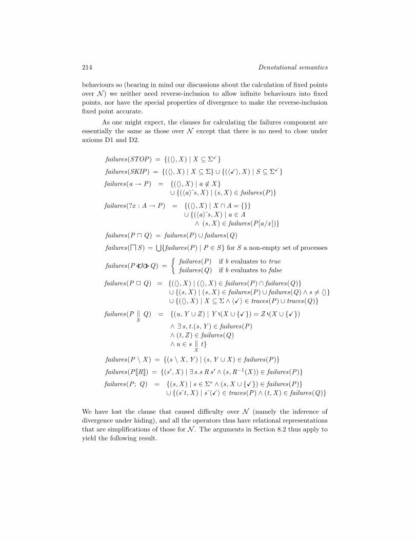
214 Denotational semantics
behaviours so (bearing in mind our discussions about the calculation of fixed pointsover N ) we neither need reverse-inclusion to allow infinite behaviours into fixedpoints, nor have the special properties of divergence to make the reverse-inclusionfixed point accurate.
As one might expect, the clauses for calculating the failures component areessentially the same as those over N except that there is no need to close underaxioms D1 and D2.
failures(STOP) = (〈〉,X ) | X ⊆ Σ
failures(SKIP) = (〈〉,X ) | X ⊆ Σ ∪ (〈〉,X ) | S ⊆ Σfailures(a → P) = (〈〉,X ) | a ∈ X
∪ (〈a 〉 s ,X ) | (s ,X ) ∈ failures(P)
failures(?x : A→ P) = (〈〉,X ) | X ∩ A = ∪ (〈a 〉 s ,X ) | a ∈ A∧ (s ,X ) ∈ failures(P [a/x ])
failures(P Q) = failures(P) ∪ failures(Q)
failures(S ) =⋃failures(P) | P ∈ S for S a non-empty set of processes
failures(P<I b>I Q) =
failures(P) if b evaluates to truefailures(Q) if b evaluates to false
failures(P Q) = (〈〉,X ) | (〈〉,X ) ∈ failures(P) ∩ failures(Q)∪ (s ,X ) | (s ,X ) ∈ failures(P) ∪ failures(Q) ∧ s = 〈〉∪ (〈〉,X ) | X ⊆ Σ ∧ 〈〉 ∈ traces(P) ∪ traces(Q)
failures(P ‖X
Q) = (u,Y ∪ Z ) | Y (X ∪ ) = Z (X ∪ )∧ ∃ s , t .(s ,Y ) ∈ failures(P)∧ (t ,Z ) ∈ failures(Q)∧ u ∈ s ‖
Xt
failures(P \ X ) = (s \ X ,Y ) | (s ,Y ∪ X ) ∈ failures(P)
failures(P [[R]]) = (s ′,X ) | ∃ s .s R s ′ ∧ (s ,R−1(X )) ∈ failures(P)failures(P ; Q) = (s ,X ) | s ∈ Σ∗ ∧ (s ,X ∪ ) ∈ failures(P)
∪ (s t ,X ) | s 〈〉 ∈ traces(P) ∧ (t ,X ) ∈ failures(Q)
We have lost the clause that caused difficulty over N (namely the inference ofdivergence under hiding), and all the operators thus have relational representationsthat are simplifications of those for N . The arguments in Section 8.2 thus apply toyield the following result.

8.4 The stable failures model 215
Theorem 8.4.2 All CSP operators are monotonic and continuous over F withrespect to the subset order, and are fully distributive.
In some ways F is better thought of as a refinement of T than as an approx-imation to N : equivalence of processes over F implies equivalence over T , whereasno such relationship exists between N and F . It is, however, vital that we un-derstand how a process’s representations in N and F are related. The followingparagraphs attempt to set this out.
• It is important to realize that, while you can sometimes tell from the shape ofa member of F that it must diverge after a trace (specifically, when there areno failures associated with the trace), you can never infer that it must not.In particular, any simply divergent process like div, µ p.p or µ p.SKIP ; p isidentified with F , and P F = P for all P .
• This same example shows the type of process for which F gives more distinc-tions than N : since P div can diverge immediately it is identified with ⊥Nover N . In other words, F lets us see the details of behaviour after possibledivergence, whereas axioms D1 and D2 force us to obscure this in N .
• We previously noted that the denotational semantics for CSP over N is onlyaccurate for finitely nondeterministic processes. Since the problem whichcaused that restriction does not arise over F , neither does the restriction.
• Since, for divergence-free processes, failures(P) = failures⊥(P), it followsthat the representations of such processes in the two models are congruent inthe obvious sense. It is this fact that leads to the most common use of F withFDR, namely that if the processes Spec and Imp are known, or postulated,to be divergence-free, then the refinement check Spec F Imp is equivalentto the less efficient Spec FD Imp.
It is the fact that F lets us see past potential divergence that gives it someuses which are more interesting than as a way of speeding up certain checks over N .The first is in situations where divergence is difficult to exclude, and it is naturalto build a system which is correct in other respects before addressing it. Here itmay be natural to formulate and establish correctness conditions over F (dealingwith safety properties and stable refusals), before making some final refinement toexclude divergence. (This is another application of the idea of stepwise refinement :see page 47.) A good example of this is in dealing with communications protocolswhich, like the Alternating Bit Protocol (Section 5.3), are designed to deal witharbitrary message loss, and perhaps duplication. In our earlier presentation of thatprotocol we built a model of the lossy communication medium which placed a fixedbound on how many consecutive messages can be lost and how many times one

216 Denotational semantics
can be duplicated, using the processes CN (in, out) to model the channels. Eventhough the protocol is designed to work for arbitrary but finite loss or duplication.For any N , the above medium is obviously a refinement of the process C (in, out)as defined on page 132 which can misbehave as much as it likes. An alternative andequivalent definition of this is:
C (in, out) = in?x → C ′(in, out , x )
C ′(in, out , x ) = out !x → C ′(in, out , x ) in?y → C ′(in, out , y)
If you replace the CN medium processes by C in the system, which wecan term ABPN , defined in Section 5.3 (constrained, as described there, to avoiddivergence in the absence of error), the result is a process ABP∞ that can diverge,but which satisfies the specification COPY (i.e., a one-place buffer) over F :
COPY F ABP∞
If checked on FDR, this will have substantially fewer states than does ABPN foreven small values of N .
This proves very cleanly that unless ABP∞ diverges, it does what we want.The monotonic and transitive properties of refinement imply that this remains truewhenever the C∞ processes are replaced by refinements such as CN . So
(i) all that remains to be proved for such a refinement is divergence freedom,and
(ii) it demonstrates that the only reason any limit is needed on the misbehaviourof the medium processes in the ABP is to avoid divergence.
The steps we have gone through in the above argument are summarizedbelow, hopefully showing how it should be reworked for other examples.
• First build a system ABP∞ such that
COPY F ABP∞
• Then find a divergence-free ABP ′ such that
ABP∞ F ABP ′
(established in this case by properties of refinement)

8.4 The stable failures model 217
• This allows us to infer that
COPY FD ABP ′
The second distinctive use of F arises when we want to establish a propertyof a divergence-free process P by analyzing not the process itself, but some contextC [P ] which involves hiding and can therefore potentially introduce divergence. Aslong as you are well aware of the existence of such divergences and what theymean, they frequently do not represent an undesirable behaviour of the underlyingprocess P . Usually the context and hiding represent some mechanism wherebyevents irrelevant to the specification can be abstracted away. Abstraction is a veryimportant subject, and Chapter 12 is devoted to it, including some uses of the ideawe are now investigating. We will therefore content ourselves with a simple butimportant one here.
In Section 13.1.1 it is stated that a process P is deadlock-free if and onlyif P \ X is, though the hiding can introduce divergence. Operationally, this isclearly true since all we care about there for deadlock freedom is that each reachablestate has an action available: it does not matter what the name of the action is.Nevertheless this result is not one of N , since in that model the introduction ofdivergence results in the assumption of deadlock via D2. It is, however, true in Fand should therefore be regarded as a statement in that model. The most interestingX to try in the above statement is Σ. No matter what P is, there are four possiblevalues for P \ Σ:
• F , indicating that P \ Σ must diverge, or in other words P can neitherdeadlock nor terminate;
• (〈〉, (〈〉,X ) | X ⊆ Σ) (equivalent in F to STOP) indicating that Pcannot terminate, but can reach a deadlock state;
• SKIP , indicating that P can terminate and cannot deadlock before it hasdone so (though since P \ Σ might diverge, this does not imply that it musteventually terminate); and
• SKIP STOP , meaning that P can deadlock and can terminate.
The statement ‘P is deadlock-free’ is thus equivalent to the assertion SKIP F P \Σ. In the majority of cases where there is no possibility of P terminating, this canbe replaced by F F P \ Σ. Of course, this is curious since what we are in effectdoing here is stipulating that a process (P \ Σ) must diverge, so we have moveda long way from the treatment of divergence over N . It is also of great practicalimportance since in FDR one usually gets much better compression of processeswhen events are hidden than without the hiding (see Section C.2).

218 Denotational semantics
The definition and theory of restriction operators over F are similar to thoseover N : (T ,F ) ↓ n = (T ′,F ′), where
T ′ = s ∈ T | #s ≤ nF ′ = (s ,X ) ∈ F | #s < n ∨ (s = s ′ 〈〉 ∧#s = n)
P ↓ n thus contains all the traces of length ≤ n and, like with N , only identifies therefusals of strictly shorter traces except for the special case dealing with conditionT3.
Exercise 8.4.1 Find an example of a process such that s | (s,X ) ∈ failures(P) isnot prefix closed.
Exercise 8.4.2 Find a single CSP process which is mapped to the bottoms (under) of T , N and F by the respective semantics.
Exercise 8.4.3 Find the least upper bound in F of the processes
(a → STOP) (b → STOP) and a → STOP
Find its representation in the model and a CSP expression with the given value.
Exercise 8.4.4 Suppose P is any process whose traces are contained in Σ∗ (i.e., it is-free). What can you say about the traces and failures of the process P ||| div?
Harder: Achieve the same effect for a process P that can terminate (though, if it helps,you can assume there is a given a ∈ Σ that P never communicates).
8.5 Notes
The central role given to semantic models such as those seen in this chapter is thething that most characterizes the theoretical treatment of CSP in relation to thoseof other process algebras. In a sense that will be made formal in the next chapter,the CSP semantic models each define a congruence which is the coarsest possiblesubject to some natural criterion. Other process algebras have found their own wayto capture failures-style equivalences, most notably the testing equivalences for CCSdescribed by Hennessy and de Nicola [32, 51].
The traces model of CSP was introduced by Hoare in [55]. This was refinedinto the failures model developed by Hoare, the author and Brookes in [18]. Thatmodel was basically N without the divergence component, and used the refinement(reverse containment) order to compute fixed points: it identified µ p.p with Chaos .That model failed to give a consistent model of divergent processes, leading, forexample, to the failure of a few of the basic laws. This was corrected with theintroduction of the divergences component in [101], [15] and [19].

8.5 Notes 219
The formulation of the model in this book is different in two ways from thatin these papers (the latter also being essentially the same one that Hoare used inhis text [56]). The first is that the early version either specified that all refusalsets are finite (even over infinite Σ) or specified that an infinite refusal set waspresent whenever all its finite subsets were (which was, of course, effectively thesame assumption). This was necessary to make the model a cpo under the refine-ment order (corresponding to the observation we made on page 199 that N overinfinite Σ is incomplete). It meant that the model could not handle unboundedlynondeterministic operators like infinite hiding at all. This assumption has beendropped in this book because (i) the later development [104] of the strong orderreferred to on page 199 means that we do not need N to be complete under to get fixed points and (ii) the development of the infinite traces extension of Nthat we will meet in Chapter 10 means that we can now unequivocally deal withunbounded nondeterminism and it is nice to have the projection function from thericher model cleanly defined. (Neither of the two equivalently powered restrictionson refusal sets mentioned above makes any sense over the infinite traces model. Soto use them over N would leave us with a real problem when it came to decidingwhich member of N was the image of a general member of the other model.)
The second change is in the handling of termination . The early modelsand CSP semantics did not special-case this nearly so much as we have done. Theconsequences of this were that sequential composition did not have some desirableproperties such as P ; SKIP = P and that some semantics did not make all ’sfinal. So axioms F4 and D3 are new here. It has long been recognized that thetreatment of termination in CSP was something of a compromise: the recent paper[129] points out one problem with the old approach (as well as providing a mostinteresting study of the automated proof of many theorems about CSP models andsemantics). See [1] for an alternative approach to representing termination in aanother process algebra.
The effects on the semantics and models of a move to an imperative (i.e., non-declarative) view of process state can be seen in [102] (where occam is considered).The primary effect is on the representation of termination, since a process now hasto be able to pass its state to its successors upon terminating.
The stable failures model F is a much more recent development. The authorhas seen a number of attempts (generally unsuccessful) over the years at eliminatingthe divergence-strictness of N . Characteristically this involved interpreting a diver-gence as equivalent to a refusal of the whole alphabet, but discarding the axiom D1which enforces extension-closure of divergence sets. That approach does not workbecause it is hard to compute fixed points accurately and various standard laws areinvalidated. The idea of simply ignoring divergence was suggested to the authorin 1992 by Lalita Jategoankar and Albert Meyer, and the model F as described in

220 Denotational semantics
this book is a result of that conversation and subsequent collaboration between theauthor and these two people. A very similar model was described by Valmari in[132].
2005: Over the past few years there has been interest in a wider range of CSPmodels. Christie Bolton showed how non-standard CSP-like equivalences could beused for capturing notions such Z refinement. There has been more interest in therefusal testing model of CSP [86] (based on [91]). New and interesting equivalences[116] have just come to light (based on work by Rehof and Rajamani) in which aprocess is modelled by its deadlock traces, its revivals (namely triples (s ,X , a) where(s ,X ) is a stable failure and a is an event that can be performed from the same statewhere X is refused, and either traces or (strict) divergences.

Chapter 9
Analyzing the denotational models
In this chapter we look in a bit more detail at the structure of the denotationalmodels we saw in the previous chapter, especially that of N . The aim is to conveysomewhat deeper understanding of the models and how they represent CSP.
9.1 Deterministic processes
The deterministic processes D, (as a subset of N ) are important both for practicaland theoretical reasons. The most obvious practical benefit from having a deter-ministic process is that it is, in some sense, testable because its behaviours, whenused over and over again, do not vary unless it is given different external stimuli.We will see in Section 12.4 that the concept can be applied in characterizing suchproperties as information flow.
The full expressive power of N is required to judge whether or not a processis deterministic. Practically no useful information can be obtained from the tracesmodel T , and the stable failures model F is inadequate because it does not modeldivergence and will equate P F with P whether P is deterministic or not. Ofcourse, for processes known to be divergence-free, one can1 test for determinismin F since the representation is then effectively the same as the one in N . Moregenerally, we can define a process to be F-deterministic if its representation in Fsatisfies the obvious condition:
t 〈a〉 ∈ traces(P)⇒ (t , a) ∈ failures(P))
This set of processes is closed under refinement and includes F . Since it does allow
1In practice it is usually better to test a process for divergence freedom and then (assumingthis works) for determinism over F .

222 Analyzing the denotational models
some usually undesirable processes, this condition is mainly of technical interest,but it does have at least one practical use – see page 330.
We have already seen that members of D play a special role in N because, asstated in Section 8.3.1, they are the maximal elements under the refinement order.In this section we establish this and other important properties of D. We first showthat every member of D is maximal; the proof that they are the only maximalelements will follow later.
Lemma 9.1.1 Every member of D is maximal (under ) in N .
Proof Suppose F are the failures of one member of D, and F ′ ⊆ F are the failuresof another process (we do not have to worry about divergences since deterministicprocesses do not have any). We have to show that F ′ = F ; first we show traces(F ) =traces(F ′). If not, there is s 〈a〉 of minimal length in traces(F ) traces(F ′) (notingthat thanks to condition F1 the empty trace does not have this property); by thisminimality we have (s , ) ∈ F ′, so by condition F3 of F ′ we then have (s , a) ∈ F ′;but since F ′ ⊆ F we also have (s , a) ∈ F , contradicting determinism of F . Thusthe trace-sets are equal; it follows by F2 that if F = F ′ there is (s ,X ) with X = such that (s ,X ) ∈ F F ′. We know (s , ) ∈ F ′; if a ∈ X then (s , a) ∈ Fby F2 and hence s 〈a〉 ∈ traces(F ) by determinism. It follows that X ⊆ a |s 〈a〉 ∈ traces(F ′) which together with condition F3 yields a contradiction to ourassumption that (s ,X ) ∈ F ′.
A deterministic process is completely characterized by its traces, becauseonce we know initials(P/s) we know refusals(P/s). Not quite all members of T giverise to a deterministic process, because of the special treatment of : a deterministicprocess that can decide to terminate immediately must do so, and so cannot offerany other choices of event.
Lemma 9.1.2 The deterministic processes are in 1–1 correspondence with the sub-set T d of T consisting of those members satisfying
s 〈〉 ∈ P ⇒ ¬∃ a ∈ Σ.s 〈a〉 ∈ P
in the sense that traces⊥(P) ∈ T d for every P ∈ D, and there is exactly one suchP for every member of T d .
Proof The fact that traces⊥(P) ∈ T d is an immediate consequence of the axiomsof N : if s 〈〉 and s 〈a〉 were both members of traces⊥(P) (for s ∈ Σ∗ and a ∈ Σ)then (s , a) ∈ failures⊥(P) by axioms F4 and F2, in contradiction to determinacyof P .

9.1 Deterministic processes 223
If Q ∈ T d , we have to find a member of D with this as its set of traces. Thisis det(Q) = (F , ), where
F = (s ,X ) | s ∈ Q ∧ X ⊆ Σ a | s 〈a〉 ∈ Q
It is easy to show that this has the required property. Since the failures in det(Q)are precisely the ones implied by axiom F3 for the given set of traces, it follows thatany other process P ′ with the same set of traces satisfies P ′ det(Q). Since weknow that deterministic processes are maximal, it follows that P ′ ∈ D, establishingthat det(Q) is the only one with the given set of traces.
Now, if P is any member of N , it is not hard to see that
P det(s ∈ traces⊥(P) | (s ′ < s ∧ s ′ 〈〉 ∈ traces⊥(P))⇒ s = s ′ 〈〉)
The set of traces on the right above are those of P which do not result as con-tinuations of traces on which P could also terminate. Thus every process has adeterministic refinement, and in particular we can easily deduce the following.
Lemma 9.1.3 If P is a -maximal element of N , then P ∈ D.
When we introduced CSP operators in earlier chapters we often said eitherthat they could, or could not, introduce nondeterminism. This idea can now begiven a precise meaning: an operator can introduce nondeterminism just when itcan produce nondeterministic results when applied to member(s) of D. In eachcase the result corresponds to the intuition we developed earlier: prefixing (a → ·)and prefix choice (?x : A → ·) both preserve determinism, as do 1–1 renaming,alphabetized parallel (P X ‖Y Q) and sequential composition (P ; Q). The lastof these holds because a deterministic P never has any alternative to the event when the latter is possible. The rest of the standard operators can introducenondeterminism:
• (a → STOP) (a → a → STOP) is nondeterministic because the initials ofthe two deterministic arguments are not disjoint. In general, if P and Q aredeterministic, ∈ initials(P)∪initials(Q) and initials(P)∩initials(Q) = ,then P Q is deterministic.
• The nondeterministic choice operator obviously introduces nondetermin-ism!
• A non-injective renaming can introduce nondeterminism when it identifiestwo visible actions from some state: for example, if f (a) = f (b) = a then
f ((a → STOP) (b → b → STOP))

224 Analyzing the denotational models
is nondeterministic.
• A parallel operator that, for any event a, allows either argument to performa independently of the other, can introduce nondeterminism because whenwe see a we cannot be sure which side it came from. Thus, for example,
(a → STOP) ||| (a → b → STOP)
is nondeterministic because, after the trace 〈a〉, the event b may be eitheraccepted or refused.
• Hiding introduces nondeterminism because it turns visible choices into inter-nal actions, and can thus, amongst other things, emulate the behaviour of:
((a → c → STOP) (b → d → STOP)
)\ a, b =
c → STOP d → STOP
D is a closed subset of the metric space N , because whenever a process Pfails to be deterministic, there is some trace s which is either a divergence or, afterwhich, P has the choice of accepting or refusing some action a. Thus if n = #s + 1then
Q ↓ n = P ↓ n ⇒ Q is nondeterministic
The rule of metric fixed-point induction, which we will meet shortly (page 229) canthen be applied to deduce the following result.
Lemma 9.1.4 If µ p.F (p) is a constructive recursion such that, whenever Q is de-terministic then so is F (Q), then the unique fixed point of F is also deterministic.
Furthermore, any constructive mutual recursion P = F (P) such that eachcomponent of F (Q) is deterministic when all components of Q are, has all compo-nents of its fixed point deterministic.
What this basically shows is that guarded recursion does not introduce non-determinism. Thus, any process definition using only
• deterministic constant processes (such as STOP and SKIP),
• operators that preserve determinism,
• other operators in cases that do not introduce nondeterminism, and
• constructive recursions

9.1 Deterministic processes 225
τ τa a a
a
a
a
Figure 9.1 Two examples of ‘nondeterministic’ LTSs whose behaviour is deter-ministic.
is guaranteed to create a deterministic process.
The definition of determinism over N takes a broad view of a process, in thesense that it looks at its set of observable behaviours rather than the way it evolvesoperationally. It is easy to devise rules which ensure that a labelled transitionsystem behaves deterministically, and one such set follows. Except for the lastcondition you can determine their truth or falsity by examining the transitions ofindividual nodes.
• No node has multiple branching on any action (visible or invisible); thusP x−→ Q and P x−→ Q ′ implies Q = Q ′.
• If a node P has a τ or action, then it is the only action of P .
• There is no infinite sequence Pi of nodes such that Piτ−→ Pi+1.
The result of mapping any node of such a system to N is certain to be deterministic,but the reverse is far from the truth. In other words, there are LTSs whose localstructure looks nondeterministic but which actually create processes that behavedeterministically. Trivial examples are shown in Figure 9.1. A much more complexone is provided by communication protocols such as the Alternating Bit Protocol(Section 5.3) in which the effects of a nondeterministic communication medium arefactored out by the way it is used, creating an overall deterministic effect. Animportant application of this possibility will be found in Section 12.4.
So it is not possible to decide whether a process is deterministic or not justby looking at the individual nodes of an LTS. There is an interesting algorithmfor deciding this question, however, which takes advantage of the maximality ofdeterministic processes under refinement. This is set out below, both for its intrinsicimportance and because it helps to illustrate some of the other ideas in this section.

226 Analyzing the denotational models
Suppose we have a process P , presented as a finite-state LTS (V ,→,P0), andwe want to know whether or not it is deterministic. By (perhaps partially) exploringthe LTS we attempt to select a subsystem (V ′,→′,P0) (with the same root node)representing a process P ′ which refines P and which meets the conditions quotedabove for being a deterministic LTS. This is done as follows:
• Initially we place P0 in V ′ and begin the search there.
• If we have to explore the node Q , then if it is stable (has no τ or action)we select for each action a ∈ initials(Q) a single node Q ′ such that Q a−→Q ′, add this transition to the subsystem and add Q ′ to the search if it isnot already in V ′. This choice means that the initial actions of Q in thesubsystem are the same as they were in the original, but that all possibilityof nondeterminism arising from ambiguity has been removed.
• If a node Q is not stable then select a single τ or action Q x−→ Q ′ andmake this action the only action of Q in the subsystem. This Q ′ is added tothe search if not already in V ′.
• If a loop of τ actions is thus encountered, we have discovered a divergenceand so can abandon the search since P is not deterministic.
This search will either eventually be abandoned because the last case arises, orterminate because all the nodes added to V ′ have been explored. If it does terminatethen the subsystem it produces is deterministic by construction and the processrepresented by each node refines the corresponding node in (V ,→,P0).
The algorithm above sometimes leaves a great many choices open about howto resolve a process’s nondeterminism, meaning that from a given system (V ,→,P0)it might choose many different subsystems, perhaps with large differences in sizeand shape. This is illustrated in Figure 9.2, where two different selections (B andC) are made from a process (A) that is, in fact, deterministic. Thus the existenceof these choices does not indicate that the original process P was nondeterministic.What we can guarantee, in any case, is that we have a deterministic process P ′ suchthat P FD P ′.
If P is deterministic then P = P ′ (even though the transition systems repre-senting these members of N may be very different) because deterministic processesare maximal. If P is not deterministic then P = P ′ and hence P ′ FD P . Thus P isdeterministic if, and only if, P ′ FD P , something we can decide with a refinementchecker like FDR. Indeed, this is the method FDR uses to decide whether a processis deterministic.

9.2 Analyzing fixed points 227
τ
a
b
τ
a
τ
A
B C
aaa
b
τ
a
a
a
b
τ
a
Figure 9.2 Two different ‘deterministic’ LTSs extracted from a ‘nondeterministic’one.
9.2 Analyzing fixed points
In this section we see how understanding the structure of semantic models allowsus to justify existing rules for proving properties of recursions and derive new rules.
At various points we have found it useful to be able to apply rules suchas fixed-point induction and UFP for inferring properties of processes. We havealready seen how UFP is justified using metric spaces, but have not proved thefixed point induction rule set introduced in Section 5.1.
Fixed-point induction If P = F (P) is any recursive definition of a vector ofprocesses which is either constructive or makes each component divergence-free,with indexing set Λ and Q ∈ NΛ is such that Qλ FD F (Q)λ for all λ ∈ Λ, then

228 Analyzing the denotational models
we may conclude that Qλ FD Pλ for all λ ∈ Λ. In the cases of F and T
this principle holds without the need to assume the constructiveness or divergence-freedom of the recursion.
The above is a good starting point for our discussion, since it is really acombination of several results requiring quite different proofs. We will look at threedifferent approaches to fixed point analysis.
Order-theoretic analysis
Sometimes one can simply use the fact that a recursive process is identified withthe least fixed point of a monotonic function f in some cpo (M ,≤). The followingis a list of a few simple arguments which can often be applied. See Appendix A formore discussion and their proofs.
• If x ≥ f (x ) then µ f ≤ x .
• If x ≤ f (x ) then f has some fixed point y (not necessarily the least) suchthat x ≤ y .
• If µ f is maximal in M , then it is the unique fixed point.
An immediate application of the first of these is the proof of the fixed-pointinduction rule for T and F . For there the refinement order is the reverse of theone used to compute fixed points, so Q F (Q) is equivalent to Q ≥ F (Q). Thisimplies µF ≤ Q , which is equivalent to µF Q , justifying the rule for thesemodels.
Metric methods
The Banach fixed point theorem, with its ability to force convergence to the uniquefixed point from any point in the underlying space, often makes it possible to achievemore powerful results about constructive recursions than about general ones. In thecase of fixed-point induction, it allows us to formulate a rule which applies to a muchwider class of properties than that specified in the definition of the rule above.
Let X be any space with a family of restriction operators defined over it thatgive a complete metric (a complete restriction space). In general, a predicate R(·)on X (i.e., a function from X to true, false) can be thought of as a subset Y of X(the members of X satisfying it). If Y is both closed (in the metric space) and non-empty, then it is a complete metric subspace of X . If f : X → X is constructive,and f (Y ) ⊆ Y , then we can regard f as being a contraction map from Y to itself,which implies that f has a fixed point in Y . But since f only has one fixed point

9.2 Analyzing fixed points 229
in the whole of X , it must be the same one. (See Exercises A.2.1 and A.2.2 foranother view of this.)
The subset Y is closed (see the Appendix) if and only if any x ∈ Y can beseen not to be a member by some finite depth of the restriction process. This canbe paraphrased as follows:
Definition The predicate R(·) on the complete restriction space X is continuousif, whenever ¬R(x ), there exists n ∈ N such that, for all y ∈ X , y ↓ n = x ↓ nimplies ¬R(y).
The demonstration that the fixed point of f , under suitable assumptions,belongs to Y then immediately implies the truth of the following rule:
Metric fixed-point induction Suppose R is a continuous, satisfiable (i.e., x |R(x ) is non-empty) predicate on the complete restriction space X . Then if theconstructive function f is inductive in the sense that, for all x ∈ X ,
R(x ) ⇒ R(f (x ))
then R(y), where y is the unique fixed point of f .
This justifies the ‘constructive’ case of the original fixed point rule, since, forany Q ∈ NΛ the predicate
R(P ′) ≡ Q FD P ′
is continuous. To see this, notice that if Q FD P ′ there must be a λ ∈ Λ and abehaviour of P ′
λ not belonging to Qλ; you can choose any n larger than the length ofthis behaviour. Note that the predicate above is always satisfiable (being satisfiedby Q) and inductive by the assumptions of the rule and monotonicity.
Whereas the standard fixed-point induction rule only allows us to prove be-havioural properties, the metric rule allows us to address properties that do nothave a characteristic process. This generalization is frequently unnecessary sincemost properties one typically wants to prove are behavioural, but it does allow usto deal with abstract specifications such as ‘deterministic’, as we saw on page 224.
Exercise 9.2.1 Suppose R and f satisfy the conditions of the metric fixed-pointinduction rule and that Q is the fixed point of f . Let P be any process satisfying R.Prove by induction that f n(P) ↓ n = Q ↓ n, and hence use the definition of a continuouspredicate to show that R(Q) holds. (This gives a more direct proof of the validity of therule than the one which explicitly uses the properties of metric spaces.)
Exercise 9.2.2 Fixed-point induction, stated informally, might be ‘if a recursive pro-cess meets some specification R on the assumptions that all recursive calls do, then it meetsthe specification unconditionally’. There are, however, three conditions that are required

230 Analyzing the denotational models
of the recursion/specification pair to make this valid: the specification must be satisfiable,the specification must satisfy some continuity condition, and the recursion must satisfysome well-formedness condition (such as being constructive).
The first of these is trivially necessary: without it, the rule would prove the pred-icate ‘false’ true of any recursion! Find examples to show that the other two are neededas well.
Exercise 9.2.3 Show that, over N , the predicates R1(P) ≡ P Q , R2(P) ≡ P Qand R3(P) ≡ P = Q are all continuous when Q is any process. Show that R4(P) ≡ P = Qis only continuous if Q = Q ↓ n for some n.
Exercise 9.2.4
(a) Suppose that R is a continuous predicate and that G and G ′ are non-destructivefunctions (all over one of the models T , N or F). Show that the predicates R(G(P))and G(P) G ′(P) are continuous.
(b) Hence show that if F is a constructive function, and H a subset of Σ, such that
P ||| RUNH ∈ D ⇒ F (P) ||| RUNH ∈ D
(remembering that D is the set of deterministic processes) then Q ||| RUNH ∈ D,where Q is the fixed point of F . An important application of this result will becomeapparent in Sections 12.4 and 12.6: we will find that the predicate being used herecan be read ‘P is secure’.
(c) Similarly show that the predicate on P
(P ‖E
STOP) ||| RUN E P ||| RUN E
is continuous. In Chapter 12 this predicate will be interpreted as ‘P is fault tolerant’:see Sections 12.3 and 12.6.
The specifications quoted in parts (b) and (c) share with pure determinism the propertyof not being behavioural specifications. You may like to convince yourself of this now, orwait until studying them properly in Chapter 12.
The strong order on N
When we discovered in Section 8.3.1 that N over an infinite Σ is not a completepartial order, it was stated in a footnote that you could use an alternative andstronger order, which was complete, to calculate the fixed points. Given (i) that Ncannot model infinite nondeterminism properly, (ii) that infinite nondeterminismis unnatural to avoid with infinite Σ (because of hiding) and (iii) that there isno problem modelling these things in the infinite traces model that we will see in

9.2 Analyzing fixed points 231
Chapter 10, it can be argued that this application of the strong order is mainly ofacademic interest. However, the existence of the order is worthy of note, particularlysince it both reveals much about how recursions converge to their fixed points in Nand allows us to prove, inter alia, the final part of the fixed-point induction rule.Much more detail on the strong order, as well as proofs of results quoted in thissection, can be found in [104].
The strong order on N asserts that P ≤ Q only when divergences(Q) ⊆divergences(P) and whenever s ∈ traces(P) divergences(P) then refusals(P/s) =refusals(Q/s) and initials(P/s) = initials(Q/s). Plainly P ≤ Q implies P FD Q ,because the only traces on which the two processes can differ are ones where P candiverge and thus has all behaviours, though there are many cases where the reversedoes not hold. In a sense, this order takes the principles enshrined in axioms D1and D2 to the extreme and says that not only is divergent behaviour undefined butthat it is the only behaviour that can be ‘refined’ in moving up the order. Onecan replace any divergence with non-divergent behaviour, but cannot subsequentlyalter the result. The following summarizes some results about ≤.
Lemma 9.2.1 (a) ≤ is a partial order on N which is stronger than FD in thesense that P ≤ Q ⇒ P FD Q .
(b) ⊥N is the least element of N under ≤.
(c) If ∆ is a ≤-directed set, then⊔
≤ ∆ exists; in this case⊔
∆ also existsand the two are equal.
(d) The maximal elements of N under ≤ are precisely the divergence-freeprocesses.
The most curious feature of ≤ is that it turns out to be interchangeable withFD for the purpose of calculating fixed points: all CSP operators are monotone, thefinitely nondeterministic ones are continuous, and each CSP-definable function hasidentical least fixed points in the two orders. For details, see [104]. An immediateconsequence of this (using (d) above) is the following result:
Lemma 9.2.2 If P = F (P) is a CSP-defined recursion with indexing set Λ, andeach component of the least fixed point P is divergence-free, then it is the uniquefixed point.
This extends the class of recursions where you can use the UFP rule toessentially all well-behaved ones.
This lemma easily disposes of the last part of the fixed-point induction rulein the case where Σ is finite, since if Q FD F (Q) then F must have a fixed pointP ′ such that Q FD P ′. Obviously it must be the unique fixed point.

232 Analyzing the denotational models
The case where Σ is infinite is more difficult since we cannot argue that sincethe set
P ′ ∈ NΛ | Q FD P ′
is a cpo under FD , and F preserves this set, there must be a fixed point in it –for it is no longer complete.
It can still be justified, but (so far as the author is aware) only using argu-ments based on topology. The predicate R(P ′) = Q FD P ′ represents a closedset with respect to the δ-topology defined in [104, 107]. Results in those papers es-tablish the rule. These same two papers, especially the second, give a rather fullerexposition of the mathematics and methods of fixed-point induction.
9.3 Full abstraction
The concept of full abstraction addresses the question of how good a semantics isfor a programming language. The definition is frequently divided into two aspects.
• The semantics S[[·]] should distinguish two programs P and Q if, and onlyif, they are distinguished by some natural criterion. Usually this criterion isthe existence of some context such that one of C [P ] and C [Q ] passes, andthe other fails, some simple test.
• The model M being used should not contain large classes of elements thatare not in the image of S. Specifically, the aim is usually to show that theexpressible elements of the model are dense, in the sense that every elementis the limit of a directed set of expressible ones.
While the second of these is clearly a desirable aim in itself – the existence ofidentifiable classes of inexpressible elements in a semantic model would seem toimply a mis-match with the language – the main reason for incorporating it underthe heading of full abstraction is that it is frequently important in establishing thefirst. For having classes of elements ofM that are distinct from all expressible onescan result in problems for program terms with free process identifiers because theymight create functions only different on inexpressible values. We will study the twoaspects below.
Of necessity the constructions used in this section often get rather detailed.The author hopes that even though some readers may not want to study all theintricacies involved, they will try to understand what full abstraction is and whatthe roles of the various constructions are.

9.3 Full abstraction 233
Expressibility
Provided we take a reasonably liberal view of what the CSP language contains,demonstrating the expressibility of the members of our semantic models usuallypresents no problem.
The liberality referred to is in using rather non-constructive mathematicalobjects to do things like index mutual recursions and use as input sets. Thus theCSP we create here falls well outside the domain of ‘effective computability’. Weare thinking here of CSP as a mathematical language for describing communicatingprocesses rather than a programming language.
Proving an expressibility result like those that follow establishes that theaxioms (such as F1–F4 and D1–D3, in the case of N ) used to define the model arestrong enough, because they do not allow anything to be considered a process whichshould not be. Let us deal with each of our models in turn.
Traces model
If s is any trace in Σ∗, it is straightforward to define a CSP process Ts which hastrace s and as few others as possible:
traces(Ts) = t ∈ Σ∗ | t ≤ s
This is done by giving Ts one of the forms
a1 → a2 → . . .→ ak → STOP and a1 → a2 → . . .→ ak−1 → SKIP
depending on whether s has last member .
It follows that if S ∈ T , then S = traces(Ts | s ∈ S) which meansthat every member of T is represented by a CSP process, albeit one using a ratherartificial and infinitary nondeterministic choice construct.
We will term the process constructed above IntTS , because in some sense it
interprets the process S .
Stable failures model
Suppose (T ,F ) ∈ F . A similar, though slightly more involved, construction createsa CSP process with this value.
The trace component T can be dealt with in much the same way as in T ,except that we cannot use the simple Ts processes used above since they give riseto stable failures that will not, in most cases, be appropriate. They need to beadapted so that failures(Ts) contains nothing that is not implied by the presenceof s . In other words, we need to create processes T ′
s that are maximal under F

234 Analyzing the denotational models
subject to containing s . These are as below, bearing in mind that we can expressthe value F as any simply divergent process.
T ′〈〉 = F
T ′〈〉 = SKIP
T ′〈a 〉 s = F a → T ′
s (a = )
The situation with the failures component is slightly trickier, since there isusually no maximal process containing a failure (s ,X ). For example, consider thefailure (〈a〉, ) in the context of the processes a → STOP and a → a → STOPdiscussed on page 213. They both have this failure, but they have no commonrefinement that does.
It is necessary to concentrate on the failures which are complete in the sensethat axiom F3 does not add anything (i.e., (s ,X ) such that a ∈ Σ | s 〈a〉 ∈ T ⊆X ). The structure of the processes T ′
t 〈〉 created above mean that we can assumethat s ∈ Σ∗ and that ∈ X . (All other complete members of F are failures ofT ′
s 〈〉.) For such (s ,X ) we can define processes F(s,X ) inductively as follows:
F(〈〉,X ) = ?x : Σ X → FF(〈a 〉 s,X ) = F a → F(s,X )
Notice that the only failures of F(s,X ) occur on trace s and are of subsets of X ,and that its traces are all in T .
It is then always true that (T ,F ) = (traces(S(T ,F)), failures(S(T ,F))),where S(T ,F) is the following set of processes (noting that the first component isalways non-empty because T is):
T ′s | s ∈ T ∪ F(s,X ) | (s ,X ) ∈ F ∧ a ∈ Σ | s 〈a〉 ∈ T ⊆ X
∧ s ∈ Σ∗ ∧ ∈ X
We will term this nondeterministic choice IntF(T ,F).
So, again, every element of F is expressible as the nondeterministic choice ofa rather artificially created set of processes.
Standing back from the constructions used for T and F , and looking at justhow the processes we have constructed to model arbitrary elements of them actuallybehave, is an excellent way of understanding the limitations of these models. Afterall, these processes must be considered useless for any practical purpose! This willbe illustrated shortly.
The failures/divergences modelWith T and F we were able to deal with each constituent behaviour very nearlyon an individual basis and form a process as a nondeterministic choice at the end.

9.3 Full abstraction 235
This was possible largely because of judicious use of the -top processes in thetwo models (STOP and F ), something that is not possible over N . The use ofan infinite nondeterministic choice operator would, in any case, be of questionabletaste over N since we have already seen that this model does not treat unboundednondeterminism accurately.
It turns out that, without and the other infinitely nondeterministic opera-tors, it is impossible to model every member of N in CSP when Σ is infinite. Thereare some patterns of refusal behaviour which are allowed by the model axioms thatcannot be created without infinite nondeterminism. In fact the only ones that canbe created with finite nondeterminism are ones where, for every trace s ,
refusals(P/s) = X | ∃Y ∈ R.X ⊆ Y
for some non-empty finite subset2 R of P(Σ) (which can vary with s).
Therefore we will only deal with the case of finite Σ here. What we can thendo is to define a mutual recursion over the whole of N : in other words, we defineone process for each (F ,D) ∈ N .
IntN(F ,D) =
⎧⎪⎪⎪⎪⎪⎪⎨⎪⎪⎪⎪⎪⎪⎩
⊥N if 〈〉 ∈ D , and otherwise
(?x : Σ X → IntN(F ,D)/〈x〉 |
X maximal in refusals(F ,D) ∧ ∈ X ∪ (SKIP<I (〈〉, ) ∈ F>I STOP)
?x : initials(F ,D) → IntN(F ,D)/〈x〉)
where ‘maximal’ means maximal under ⊆ (noting that any such refusal set iscomplete in the sense described earlier that it includes all impossible events, andthat maximal refusals must be present because of our assumption that Σ is finite).In the interest of brevity, the above definition uses the general nondeterministicchoice operator , but only over finite sets of processes where it could have beenreplaced by the binary .
You can think of this curious recursion as an ‘interpreter’ of members of Ninto CSP: at any stage the process’s state is (F ,D)/s , where (F ,D) is the initialvalue of the process and s is the current trace. The recursion is constructive, whichleads to the following remarkable argument for its correctness. We can form a vector
2Obviously this condition has to be satisfied when Σ is finite, since then (Σ) is also finite.We could, of course, have included the above property as an additional axiom for N . This wouldhave made it a cleaner model for finitely nondeterministic CSP at the expense of losing the abilityto model unboundedly nondeterministic CSP at all and making N ’s links with other models alittle more obscure.
The special properties of and axiom F4 mean that not all such R produce an allowable setof refusal sets.

236 Analyzing the denotational models
IdN of processes, indexed by N itself (i.e., a member of NN ), in which each memberis mapped to itself. This vector is easily seen to be a fixed point of the recursionand hence, by the UFP rule, equals 〈IntN
(F ,D) | (F ,D) ∈ N〉, and so
(failures⊥(IntN(F ,D)), divergences(IntN
(F ,D))) = (F ,D)
In contrast to the two models dealt with earlier, the processes IntN(F ,D) are
usually a reasonable reflection of how one would expect a process with the givenvalue to behave. As a simple example, consider the process P = a → P . If thiswere interpreted in the three models and we then applied the three constructionsto the results, the processes obtained would behave as follows.
• IntTT gives a process which performs any number of a’s and then stops. It is
the same as the process A∗ seen on page 204.
• IntF(T ,F) gives a process which makes a choice, over all n, of offering n a’s
unstably in turn and then offering a again, stably, before finally simply di-verging, and additionally has the option of offering any finite number of a’sand never becoming stable (again, diverging after the last).
• IntN(F ,D) behaves identically to the original P , simply offering a’s stably for
ever.
Distinguishing processes
The second thing we have to do is find what criteria for distinguishing processes bestcharacterize each of our models. It is certainly reasonable to argue that the simpleconstruction of the models from process behaviours makes this unnecessary3: thesets of behaviours are easy to understand and processes are identified if and only ifthey have the same ones. But these criteria can be simplified yet further if we usethe full power of how full abstraction is formulated: P must equal Q if and onlyif C [P ] and C [Q ] always (i.e., for all contexts C [·]) either both satisfy or both failthe tests.
Hopefully the following arguments will help the reader to understand theconcept of full abstraction, as well as further exploring the expressive power ofCSP.
3The concept of full abstraction is more vital on semantics using models which have a moresophisticated structure than simple sets of behaviours, frequently being applied to ones recursivelydefined using domain theory. There are some languages, such as the typed λ-calculus, for whichit is famously difficult to find a fully abstract semantics.

9.3 Full abstraction 237
Traces model
Select any member of Σ. It is convenient to give it a suggestive name such as fail .We can then formulate a simple test on processes: they fail it when they have thetrace 〈fail〉 and pass it otherwise. Call this test T1.
Since T1 is formulated in terms of traces, and the traces model calculatesthe traces of any CSP process accurately, it is obvious that if traces(P) = traces(Q)then C [P ] and C [Q ] either both pass or both fail it. In order to establish that thetest is strong enough to distinguish all pairs of processes, we need to show thatwhenever traces(P) = traces(Q) there is a context C [·] such that one of C [P ] andC [Q ] passes, and the other fails, it. We can achieve this by finding, for any traces , a context CTs [·] such that CTs [P ] fails T1 precisely when s ∈ traces(P). Thereare various ways to do this; one is set out below.
• When s = s ′ 〈〉, a simple context that does what we want is
CTs [V ] = (V ‖Σ
Ts) \ Σ; (fail → STOP)
where Ts is the same process used on page 233 in exploring expressibil-ity. The point is that the process on the left-hand side of the sequentialcomposition can only terminate when V has completed the trace s .
• For s ∈ Σ∗, we can use the context
CTs [V ] = ((V ‖Σ
Ts)[[a/x | x ∈ Σ]] ‖a
FAIL(#s)) \ a
where again Ts is as used for expressibility, a is any member of Σ distinctfrom fail , and FAIL(m) is defined
FAIL(m) = (fail → STOP)<I m = 0>I (a → FAIL(m − 1))
This context, much as with the more obvious first case, works by only allowingthe trace s to occur in V and, like the first one, communicating fail onlywhen it is complete and its contents hidden.
This establishes that the traces model is, indeed, fully abstract with respectto the simple test chosen.
Stable failures model
One might expect the tests used for F to be a refinement of the method used above,and in order to distinguish processes on the basis of refusals it is clearly necessarythat some aspect of the tests involves more than observing traces. We have two

238 Analyzing the denotational models
types of behaviour to handle: traces and failures. It is possible to combine twoseparate forms of test, one for each type, into one by disjoining them: let us definetest T2 to fail if a process either can communicate fail as its first action or deadlocksimmediately (i.e., stably refuses the whole of Σ).
Clearly the semantics of CSP in F can accurately calculate whether anyprocess fails T2, and so all we have to do to establish full abstraction is to showthat if (T ,F ) = (T ′,F ′) are the representations of processes P and Q then thereis a context that distinguishes them (with respect to T2).
Suppose first that T = T ′. Then the context we use is a slightly modifiedversion of the one used for T . For any trace s ∈ Σ∗, let
CT ′s [V ] = CTs [V ] ||| F
This has identical traces but, since it is never stable, will never fail T2 becauseof deadlock. Thus CT ′
s [Q ] fails T2 exactly when CTs [Q ] fails T1, which is whens ∈ traces(Q). This form of context thus allows us to distinguish two processeswith unequal trace sets.
We can thus assume that T = T ′ and F = F ′. So let s be a trace such thatrefusals(P/s) = refusals(Q/s). It is easy to show that s is not of the form s ′ 〈〉.
Without loss of generality we can assert there is a refusal set X such that
• (s ,X ) ∈ F F ′
• a ∈ Σ | s 〈a〉 ∈ T ⊆ X
• ∈ X , because if s 〈〉 ∈ T , then by F4 the sets of refusals of P and Q notcontaining are identical.
Consider the context
CF(s,X )[V ] = ((V ; F ) ‖Σ
F(s,Σ X )) \ Σ
where F(t,Y ) is the process used when investigating expressibility that has thefailures (t ,Y ′) for Y ′ ⊆ Y and no other. Since we are hiding the entire alphabet ina process that cannot terminate, there are only two possible values for CF(s,X )[V ]:F or STOP , the latter being one that can deadlock and hence fail T2. CF(s,X )[P ]can fail T2 because P has the failure (s ,X ), hence so does P ; F (using ∈ X ),and so the parallel combination has the failure (s , Σ). If CF(s,X )[Q ] could fail itthen you can argue in reverse to show Q must have a failure (s ,X ′) for X ′ ⊇ X , butit cannot by our assumptions and axiom F2. Thus contexts of the form CF(s,X )[V ]allow T2 to detect differences between failure-sets.

9.3 Full abstraction 239
It is reasonable to hope that T2 might be simplified further to just testingfor immediate deadlock, but unfortunately the standard CSP language does notallow us to construct contexts that are strong enough to tell differences betweentrace-sets by this means. The problem is that if P and Q are two members of N ,neither of which can either terminate or become stable (i.e., they both have theform (T , ) for T ⊆ Σ∗) then there is no context that can distinguish them on thebasis of deadlock. There is no way for P to make a significant contribution to thebehaviour of C [P ], and for the context subsequently to become stable, for none ofthe standard operators of CSP can ‘switch off’ P .
It is easy to add an operator to CSP which rectifies this situation: an in-terrupt operator which allows one process Q to take over from another P . This iseasiest to understand for a specified event i being the signal for Q to start: P i Q .The semantics of this operator over F are:
traces(P i Q) = traces(P)∪ s 〈i 〉 t | s ∈ traces(P) ∩ Σ∗ ∧ t ∈ traces(Q)
failures(P i Q) = (s ,X ) ∈ failures(P) | s ∈ Σ∗ ∧ i ∈ X ∪ (s ,X ) | s 〈〉 ∈ traces(P) ∧ ∈ X ∪ (s 〈〉,X ) | s 〈〉 ∈ traces(P)∪ (s 〈i 〉 t ,X ) | s ∈ traces(P) ∩ Σ∗
∧ (t ,X ) ∈ failures(Q)
Given this operator, it is not too hard to devise a context that will allowC [P ] to deadlock immediately, precisely when P has a specified trace s ∈ Σ∗, andto deal with traces of the form s 〈〉 using sequential composition in a similar way.This then leads quickly to the aimed-for full abstraction result. The details are leftas an exercise. See Exercise 9.3.2 for an investigation of a related result.
We can learn an important lesson from this: adding or removing constructsfrom a language, even when the semantic model is unchanged, can greatly affectfull abstraction properties.
Failures/divergences model
With N there seems to be no option but to use a disjunctive test in the samespirit as T2. This is T3, which a process fails if it either immediately diverges orimmediately deadlocks. Following in the footsteps of the earlier models, to showthat T3 is strong enough we need to find a context to distinguish any pair P , P ′ ofdifferent elements of N .
Let a be any member of Σ. For s ∈ Σ∗, then the context
CT ′′s [V ] = (V ‖
ΣT ′′
s ) \ Σ ||| (a → STOP)

240 Analyzing the denotational models
can diverge immediately if and only if s ∈ traces⊥(V ), where
T ′′〈〉 = ⊥N
T ′′〈b〉 s = b → T ′′
s
The role of the event a in this definition is to prevent the process deadlockingimmediately and thereby failing T3 in an unexpected way.
Thus, if P and P ′ differ in whether they have this trace, they can be distin-guished. Traces of the form s ′ 〈〉 can be dealt with similarly (see Exercise 9.3.1).We can thus use T3 to distinguish P and P ′ if their trace-sets differ.
If s is a divergence of one process and not the other, then by D3 we canassume s ∈ Σ∗. After replacing the process ⊥N by STOP in the definition of T ′′
s ,we can use the same context as for traces, since the divergence that trips the testthen comes from V rather than T ′′
s .
So we can assume that our two processes have identical trace and divergencesets, and (without loss of generality) (s ,X ) ∈ failures⊥(P) failures⊥(P ′). Clearlyno prefix of s is a divergence, and exactly as over F we can assume ∈ X and thatX includes all impossible events. We use a context similar to that used for failuresover F , the important difference being that we have to use a different method toavoid it deadlocking until the chosen failure is reached. It is built in two stages.
We have to deal separately with the cases X = and X = . In thefirst case let
C(s,X )[V ] = (V ‖ Ts 〈〉); (a → STOP)
where again a is any member of Σ.
In the second case let a ∈ X and define AS = a → AS . The followingis a simplified version of the F(s,X ) seen earlier:
F ′(〈〉,X ) = ?x : Σ X → STOP
F ′(〈b〉 s,X ) = b → F ′
(s,X )
Now define
C(s,X )[V ] = (V ; AS ) ‖Σ
F ′(s,Σ X )
In either case C(s,X )[V ] behaves as follows:
• Until it has completed s (or diverged in the process, something which willnot happen when s is not a divergence of V ) its trace is always a prefix of s .

9.3 Full abstraction 241
• It may or may not be able to deadlock on proper prefixes of s .
• On the complete trace s it can deadlock if, and only if, V has the refusal(s ,X ).
What we have to do is place this process in a context which generates an immediatedeadlock from any deadlock of the above after s , but not from any other trace, anddoes not introduce a divergence. One way of doing this is
CFD(s,X )[V ] = ((C(s,X )[V ][[a, b/x , x | x ∈ Σ]]) ‖a,b
W (#s)) \ a
where
W (0) = b → CSW (n) = (a →W (n − 1)) CS (n > 0)
CS = c → CS
and a, b, c are arbitrary members of Σ.The process W (#s) keeps track of how many events C(s,X )[V ] has per-
formed, and only allows it to deadlock the combination when this number is exactly#s , meaning that C(s,X )[V ] has actually performed s . (The double renaming ofevents to both a and b, coupled with the structure of W (n), means that only eventsfrom the trace s get hidden. Thus the behaviour of V up to trace s is brought for-ward to the empty trace of the combination, but anything beyond is not. This useof one-to-many renaming appears to be essential.4) It follows that CFD(s,X )[V ]fails T3 if and only if (s ,X ) ∈ failures⊥(V ).
CFD(s,X )[V ] can then be used to distinguish P and P ′, as desired.We can summarize the results of this section in the following result:
Theorem 9.3.1 (i) The traces (T ) semantics of CSP is fully abstract with respectto T1 (failed on the immediate occurrence of a chosen event).
(ii) The stable failures (F) semantics is fully abstract with respect to T2
(failed on immediate occurrence of a chosen event or immediate deadlock), andwith the addition of an interrupt operator this test can be weakened to immediatedeadlock.
(iii) The failures/divergences (N ) semantics of finitely nondeterministicCSP is fully abstract with respect to T3 (failed on the process immediately dead-locking or diverging) provided Σ is finite.
4The construction given here is a correction from that in the first edition, which did not usethe double renaming and which was wrong because it hid the events of a process accepting anevent from Σ X as well as the ones in the trace leading up to it. The author is grateful to AnttiValmari for pointing out this error.

242 Analyzing the denotational models
Another consequence of full abstraction properties like these is that eachmodel generates the weakest congruence (i.e., identifies most processes) which allowsus to tell whether a process satisfies the relevant test. Thus T gives the weakestcongruence on CSP allowing us to tell whether a process has the trace 〈fail〉, andso on.
Exercise 9.3.1 Recall that the context CT ′′s [·] is used to distinguish processes in N
on the basis of traces. The version defined on page 239 was only for s ∈ Σ∗. Find adefinition that works for traces of the form s 〈〉.
Exercise 9.3.2 Notice that axiom T3 implies that all traces of the form s 〈〉 aretraces of failures. The only semantic clause for standard CSP operators over F in whichthe failures component depends on the input traces is P ; Q , in which only traces of thisform are used. Show that this means it is possible to give a semantics for CSP in a purestable failures model in which a process is represented only by failures(P) rather than(traces(P), failures(P)).
(a) Show that axioms F2, F4 and a much weakened F3 (dealing only with two casesthat can occur in connection with ) suffice to create a model whose membersare exactly the failure-sets that arise in F . We no longer get the full version ofF3 because it relates refusal sets to successor traces, and by leaving out the tracecomponent it thus becomes impossible to include this particular ‘sanity check’.
(b) Prove that this model is fully abstract for the standard CSP language with respectto the test for immediate deadlock.
(c) Find two processes that are identified over this new model but distinguished overboth T and F . What are the advantages of using F rather than the pure version?Are there any disadvantages?
9.4 Relations with operational semantics
We have two methods of working out the representations of CSP processes in ourabstract models: either following the route of Chapter 7 and calculating the op-erational semantics and then extracting behaviours via abstraction functions, orthat of Chapter 8 and doing it by directly using denotational semantics. There is aclaim implicit in this, namely that both ways calculate the same value. We are, inother words, claiming that the operational semantics is congruent with each of thedenotational ones. This is something that needs to be proved, and in this sectionwe outline some of the methods that can be used to do this.
Firstly, one must remark that in order to keep the discussion clear we willhave to be a little more formal than hitherto about the distinctions between thesyntax of CSP and functions defined over it. The language of terms in CSP (i.e., the

9.4 Relations with operational semantics 243
set of well-formed terms in the language that may contain free process identifiers)will be denoted CSP, and the closed terms (ones with no free identifiers) will bedenoted CSP. Naturally, when referring to a function like failures⊥(P) we willhave to make it clear which of the two supposedly equal values this is.
The operationally-based versions of these functions defined in Section 7.4.1provide us with functions to the models from any LTS V : for each node σ of V
ΦT (σ) = traces(σ)ΦF (σ) = (traces(σ), failures(σ))ΦN (σ) = (failures⊥(σ), divergences(σ))
These can, of course, be used to compute one set of interpretations of CSPfrom the LTS generated by the operational semantics. The second set are producedby the denotational semantics given in Chapter 8: let us call these ST [[·]], SF [[·]] andSN [[·]].
A variety of techniques have been used over the years to establish the equiv-alence of pairs of these interpretations. Invariably the proofs have been by somesort of structural induction over the syntax of a CSP program and come in threeparts: a series of lemmas dealing with basic operators other than recursion, a moredifficult argument to handle the recursive case, and overall ‘glue’ to put all thesepieces together. Presenting detailed arguments for each of the models here wouldbe much too long and complex, so we will concentrate on the simplest model, T ,and indicate briefly at the end how things change for the others.
A CSP term can, in general, have free process identifiers. Even if we startwith a closed term (one with none), if we want to establish results about it bystructural induction we may well have to consider sub-terms which are not closed.In proving congruence between an operational and a denotational semantics it istherefore necessary to use notation capable of interpreting general terms5 and toformulate our inductive congruence results accordingly.
It is mathematically superior to formulate each of the denotational semanticswith environments giving a binding of each free process identifier to an element ofthe underlying semantic model. (This type of environment was previously discussedon page 164.) Thus, we can define
EnvT = Ide → T
to be the set of T -environments, so that the type of the semantic function becomes
ST : CSP→ EnvT → T
5As remarked previously (for example in Chapter 7), we have avoided doing this formally up tonow. This was because the gain in terms of completeness and making the semantics of recursiontidier would have been outweighed by the notational and conceptual clutter.

244 Analyzing the denotational models
and, for a process term P and environment ρ ∈ EnvT , ST [[P ]]ρ is the value of Pwhen its free identifiers have the trace sets assigned to them by ρ. The reason whyit is superior is because, when we are faced with a recursive term such as µ p.P ,we can present the function that P represents cleanly: in a given environment ρ itmaps α ∈ T to ST [[P ]]ρ[α/p].
The natural operational semantic analogue of an environment is a substitu-tion ξ that maps each identifier to a closed CSP term:
ξ ∈ Subst : Ide → CSP
ξ then converts any CSP term P into a closed one subst(P , ξ) by replacing each freeidentifier p by ξ(p). The full statement of the congruence result is now that, for allξ ∈ Subst and all terms P ∈ CSP,
ΦT (subst(P , ξ)) = ST [[P ]]ξT
where ξT
is the member of EnvT produced by applying ΦT to each component ofξ:
ξT
(p) = ΦT (ξ(p))
It is this result we prove by structural induction over P (for all ξ simultaneously).
The claim is trivially true for all ‘base’ cases of the induction: P being eithera process identifier p or one of the constant processes STOP and SKIP .
The proof then follows the same pattern for each non-recursive operator.Consider, for example, . We can assume P and Q are two terms both satisfyingthe claim for all ξ. We have
subst(P Q , ξ) = (subst(P , ξ)) (subst(Q , ξ)), and
ST [[P Q ]]ξT
= ST [[P ]]ξT
T ST [[Q ]]ξT
where T is the representation of this operator over T , in this case ∪ (union). Thus,by induction, it is sufficient to prove that for any closed CSP terms R and S ,
ΦT (R S ) = ΦT (R) T ΦT (S )
This result, and corresponding ones for all the other operators, can be provedby analyzing how the operational semantics behaves. Specifically, in this case, it iseasy to show that, for any R and S ,
• If R〈〉
=⇒ R′ and S〈〉
=⇒ S ′ then R S〈〉
=⇒ R′ S ′.

9.4 Relations with operational semantics 245
• If s = 〈〉 and either R s=⇒ T or S s=⇒ T then R S s=⇒ T .
• The above are the only pairs (s ,V ) such that R S s=⇒ V .
This, of course, establishes what we want.
Now consider the case of a recursion µ p.P . What we have to show is that,for any ξ, ΦT (subst(µ p.P , ξ)) is the least fixed point of the function Υ mappingα ∈ T to ST [[P ]](ξ
T[α/p]). The inductive assumption makes it easy to show that it
is a fixed point. Let P ′ be the term in which all free identifiers of P other than phave been substituted by ξ, so that subst(µ p.P , ξ) = µ p.P ′. Then
ΦT (subst(µ p.P , ξ)) = ΦT (µ p.P ′)= ΦT (P ′[µ p.P ′/p]) (a)= ΦT (subst(P , ξ[µ p.P ′/p])) (b)
= ST [[P ]]ξ[µ p.P ′/p]T
(c)= ST [[P ]](ξ
T[ΦT (µ p.P ′)/p]) (d)
= Υ(ΦT (subst(µ p.P , ξ)))
(a) follows because of the operational semantics of recursion:
µ p.P ′ τ−→ P ′[µ p.P ′/p]
and because if A is a node of an LTS whose only action is A τ−→ B then ΦT (A) =ΦT (B). (b) follows by definition of P ′, (c) comes by induction on the term P whichis simpler than µ p.P , and (d) by definition of ξ
T.
Recall that, for T , we chose to identify recursions with the subset-least fixedpoints of the associated functions, arguing that this was natural because all thebehaviours recorded in this model always appear finitely. To show that this was theright decision, given the above argument, it is sufficient to show that every traceof ΦT (subst(µ p.P , ξ)) belongs to Υn(〈〉) for some n. (Containment in the otherdirection comes from the fact that ΦT (subst(µ p.P , ξ)) is a fixed point of Υ, and sois greater than the least one.)
If s is such a trace then there must be some s ′ ∈ (Στ )∗ and Q such that
s ′ \ τ = s and subst(µ p.P , ξ) s′−→ Q . If N = #s ′, then during the derivation of
the behaviour s ′, the recursion cannot possibly be unfolded more than N times,since every time it is unfolded a τ action is generated which must be present in s ′.Consider the following two mutual recursions defining the processes p0 and q0.
pn = P ′[pn+1/p] n ∈ N
qn = P ′[qn+1/p] n ∈ 0, . . . ,N − 1qN = STOP

246 Analyzing the denotational models
where P ′ is as above. The first of these clearly has exactly the same behaviour assubst(µ p.P , ξ), in the sense that the operational semantics are exactly alike exceptthat the multiple names of the identifiers in the mutual version keeps track of howmany times the recursion has been unfolded. The process q0 behaves exactly like p0
until after the N th unfolding, which means that it has the behaviour s ′; this meansthat s ∈ ΦT (q0).
On the other hand, ΦT (qN ) = 〈〉, ΦT (qN−1) = Υ(〈〉) etc., until ΦT (q0) =ΥN (〈〉), because ΦT (subst(P , ξ[Q/p])) = ST [[P ]]ξ
T[ΦT (Q)/p] for every closed
term Q . Hence s ∈ ΥN (〈〉), which is what we wanted to show.
This completes our sketch of the proof of congruence between the operationalsemantics and the trace semantics. The proof for F goes through exactly the samesteps, except that one obviously has to keep track of failures as well as traces andit is necessary to allow the q0 recursion to unfold N + 1 times rather than N .
With N there is little difference with the overall structure of the proof orthe cases for non-recursive operators. The recursive case is different because wehave to handle infinite behaviours (divergences) and use what is really the oppositefixed point. We have to show that the effects of divergence lead to the operationalsemantics mapping under ΦN to the N -least fixed point, bearing in mind thatthe same basic argument applied over T (page 245) shows that any recursive termmaps to a fixed point of the associated function.
Perhaps the easiest way of proving minimality uses Konig’s lemma (applicablesince we are in any case restricted to finitely nondeterministic CSP). For any traces ∈ Σ∗, one shows that either the tree of states reachable from a process such asR = subst(µ p.P , ξ) on prefixes of s is finite, or there is a divergence in the tree.In the second case, axioms D1 and D2 mean that every behaviour on s gets intoΦN (R), while in the first case you can limit the number N of times the recursionhas to be unfolded to be the depth of the finite tree, and then a similar argumentto that applied over T can be used to show that the operational and denotationalsemantics must agree on behaviours that are prefixes of s .
Exercise 9.4.1 Prove that, for any closed term P , ΦT (P \ X ) = ΦT (P) \T X .
Exercise 9.4.2 Repeat the previous exercise for (i) the stable failures model F and(ii) the failures/divergences model N , the latter under the assumptions that the term Pis finitely nondeterministic and X is finite.
Exercise 9.4.3 The results on expressibility in Section 9.3 imply that, in each of thecases considered, the function ΦM is surjective as a function from the closed CSP termsCSP to the model M. Show that there is a transition system V on which the function ΦN
is surjective when Σ is infinite (i.e., the one case not dealt with by the previous remark).

9.5 Notes 247
9.5 Notes
The main properties of deterministic processes have been well known since failures-type models were first developed [15, 18, 19, 101].
The results of Section 9.2 are derived mainly from [101, 104, 107]. The lasttwo of these contain the details omitted here of the purely topological approach toCSP fixed-point induction.
The notion of full abstraction evolved in the 1970s and early 1980s: see[79, 92] for example. The full abstraction result for N has been known for manyyears: it is implicitly present in [51], for example (which also contains mush othermaterial on full abstraction). The full abstraction results for F , like the other resultsabout this model, arose from the collaboration between the author, Jategoankar andMeyer, and are closely related to independent results of Valmari [132].
The first congruence proof between operational and denotational semanticsof CSP appears (rather briefly) in Olderog’s important paper [87] with Hoare. Amore complete presentation of a proof appears in [135] and [22]. The difficulty insuch proofs comes mainly from the radically different ways in which denotationaland operational semantics handle recursions. The above two references handle thisin different ways; the author later developed a further way of handling this (en-compassing unbounded nondeterminism and discontinuous functions) in [105] – thelater is the style of proof he presently prefers.
2005: Some interesting results have been proved about the properties whichcan be expressed by CSP refinement in its most general form:
F (P) G(P)
for F and G being CSP contexts [115, 112]. It turns out that the ones which can beexpressed by a natural class of contexts are exactly the properties which are closedin the usual metric space on the failures/divergences model provided the alphabet Σis finite. This can be viewed as a sort of higher-order full abstraction result.


Chapter 10
Infinite traces
We have seen (Section 8.3.2) that the failures/divergences model is deficient in theway it models infinitely nondeterministic processes. The solution is to include theset of a process’s infinite traces in the model. An infinite trace is a member of Σω,the sequences of the form 〈ai | i ∈ N〉. It represents a complete (i.e., throughout alltime) communication history of a process that neither pauses indefinitely withoutcommunicating nor terminates.
In this chapter we see how this is done and get an idea of the extra expressivepower it gives us.
10.1 Calculating infinite traces
Our aim is to represent each process by the triple
(failures⊥(P), divergences(P), infinites(P))
recalling that infinites(P) already, by definition, contains all extensions of diver-gences.
Bear in mind that we know (thanks to the argument in the proof of Theorem7.4.2 on page 178) that for any finitely nondeterministic process
infinites(P) = traces⊥(P) traces⊥(P)
where S = S ∪ u ∈ Σω | ∀ t < u.t ∈ S. Thus, the extra component will onlyconvey extra information outside this category of process.
If we are to follow the route taken in Chapter 8 we should now axioma-tize which triples (F ,D , I ) are allowable, investigate the model’s properties (order-theoretic and otherwise) and then use it to give the semantics. It is entirely possible

250 Infinite traces
to build such a model, and indeed we will do so later in this chapter, but it turns outthat the relationship in it between failures and infinite traces is remarkably subtleand creates problems which there is no overriding need for us to meet yet.
One can, at least temporarily, avoid these difficulties thanks to the followingobservations:
• The stable failures failures(P) are accurately calculated, even for infinitelynondeterministic CSP, by the semantics over the stable failures model F .
• If one examines the way that CSP operators generate behaviours, it turnsout that the stable failures of component processes never influence any offinite or infinite traces or divergences.
It therefore makes sense to introduce infinite traces via a simpler model in which aprocess is modelled as
(traces⊥(P), divergences(P), infinites(P))
We can still work out failures⊥(P) from a combination of the second componentsof this representation and the semantics over F .
I, the infinite traces/divergences model, consists of the triples (T ,D , I ),where T ,D ⊆ Σ∗ and I ⊆ Σω, meeting the following conditions:
T1. T is non-empty and prefix closed.
D1. s ∈ D ∩ Σ∗ ∧ t ∈ Σ∗ ⇒ s t ∈ D
D2′. D ⊆ T
D3. s 〈〉 ∈ D ⇒ s ∈ D
D4. s ∈ D ∩ Σ∗ ∧ u ∈ Σω ⇒ s u ∈ I
I1′. u ∈ I ∧ s < u ⇒ s ∈ T
I is a complete lattice under both I (defined, of course, to mean reverseinclusion on all three components) and its reverse, the subset order. For I =(〈〉, , ) (the representation of STOP) is the greatest I-lower bound of theempty set, and the greatest lower bound of any non-empty set is given, as usual, bycomponentwise union: S = (T ∗,D∗, I ∗), where
T ∗ =⋃T | (T ,D , I ) ∈ S
D∗ =⋃D | (T ,D , I ) ∈ S
I ∗ =⋃I | (T ,D , I ) ∈ S

10.1 Calculating infinite traces 251
The least refined element is ⊥I = (Σ∗, Σ∗, Σω), representing any process thatcan diverge immediately.
It is easy to give clauses for calculating infinites(P) for all the standard CSPoperators.
infinites(STOP) = infinites(SKIP) =
infinites(a → P) = 〈a 〉 u | u ∈ infinites(P)infinites(?x : A→ P) = 〈a 〉 u | a ∈ A ∧ u ∈ infinites(P [a/x ])
infinites(P Q) = infinites(P) ∪ infinites(Q)
infinites(P Q) = infinites(P) ∪ infinites(Q)
infinites(P ‖X
Q) = u ∈ Σω | ∃ s ∈ Traces(P),
t ∈ Traces(Q).u ∈ s ‖X
t
∪ s u | s ∈ divergences(P ‖X
Q) ∩ Σ∗ ∧ u ∈ Σω
infinites(P ; Q) = infinites(P)∪ s u | s 〈〉 ∈ traces⊥(P) ∧ u ∈ infinites(Q)
infinites(P [[R]]) = u ′ | ∃ u ∈ infinites(P).u R u ′∪ s u | s ∈ divergences(P [[R]]) ∩ Σ∗ ∧ u ∈ Σω
infinites(P \ X ) = u ′ ∈ Σω | ∃ u ∈ infinites(P).u \ X = u ′∪ s u | s ∈ divergences(P \ X ) ∩ Σ∗ ∧ u ∈ Σω
Recall that Traces(P) is an abbreviation for traces⊥(P) ∪ infinites(P). The traceconstructs ‖
X, \ X and renaming have been extended in the natural ways to encom-
pass infinite traces. Of course, to give a denotational semantics to CSP you needclauses for the other components, traces⊥(P) and divergences(P), of the represen-tation. In all but one case, the clauses for divergences(P) are the same as they wereover N because knowledge of a process’s infinite traces does not affect what thedivergences are when applying the respective operators. The exception is hiding,since we no longer have to attempt to infer what the infinite traces are from thefinite ones and can directly define:
divergences(P \ X ) = (u \ X ) t | u ∈ infinites(P)∧t ∈ Σ∗ ∧ u \ X is finite
∪ (s \ X ) t | s ∈ divergences(P) ∩ Σ∗ ∧ t ∈ Σ∗
The definitions for the finite traces component traces⊥(P) are identical tothe mappings on traces that can be extracted from the failures clauses for N . These

252 Infinite traces
differ from the clauses for the finite traces model T only in the cases where it isnecessary to close up to preserve axiom D2/D2′, so for example
traces⊥(P \ X ) = s \ X | s ∈ traces⊥(P)∪ s t | s ∈ divergences(P \ X ) ∩ Σ∗ ∧ t ∈ Σ∗
All the resulting semantic clauses are both universally accurate and repre-sentable as relations over behaviours: we have eliminated the problem which causedthe semantics over N to break down for infinitely nondeterministic CSP. It is nowpossible to prove the lemmas of an operational/denotational congruence proof (likethat for and T on page 244) for every one of the operators. For example, theprocesses A∗ and A∞ defined on page 204 are now clearly distinguished by thesemantics, which correctly predict that A∞ \ a can diverge and that A∗ \ acannot.
The fact that they are representable by relations implies (as in Section 8.2)that they are all monotonic, fully distributive, and continuous in the ⊆ order. Let usconsider the question of continuity in the order. The argument for the continuityof hiding over N no longer applies because of the different way we are calculatingdivergence. One would not expect the argument to apply when we reason aboutinfinitely nondeterministic CSP, since it relied on Konig’s lemma, which in turnrequires finite branching. And, in fact, hiding is not continuous over I. When Σ isinfinite, the same example as used on page 188 works. An example for finite Σ isprovided by the processes Qn defined below (hiding a, b makes each Qn diverge,but not their limit A∗). Indeed, the incorporation of infinite traces, which eachcontain an infinite amount of information, leads to several other relations becominginfinitary and the corresponding operators discontinuous. This applies to sequentialcomposition, parallel and finitary renaming.
For example, let R be a renaming that maps events a and b to b, and let Pn
be the process that performs n a’s and then an infinite sequence of b’s:
Pn = a → . . .→ a → BSBS = b → BS
Obviously Pn [[R]] = BS for all n. If we define Qn = Pm | m ≥ n then theseform an increasing sequence under I whose limit is actually A∗ (it can performany finite sequence of a’s, but has no infinite trace). But we then have
⊔Qn [[R]] | n ∈ N = BS = (
⊔Qn | n ∈ N)[[R]]
demonstrating the failure of continuity.
In Chapter 8 we established a rule of thumb that one should identify a re-cursion with either the or ⊆ least fixed point depending on whether or not one’s

10.1 Calculating infinite traces 253
model incorporates infinite behaviours. On this principle we must expect the rightanswer for I to be , and indeed it is, despite the fact that it means a large-scaleabandonment of continuity and the resulting simple formula for fixed points. Theneed to use rather than ⊆ can now be demonstrated not only from under-definedrecursions such as µ p.p, (which diverges and so must be mapped to ⊥I rather thanto I), but also from very ordinary ones such as µ p.a → p.
For (〈a〉n | n ∈ N, , ) (which is the value in I of the process A∗), isthe ⊆-least fixed point of the function F (·) derived from the recursion µ p.a → p.This is plainly not the right value, since it does not contain the infinite trace thatthe process self-evidently has. The problem is that F (P) can never have an infinitetrace when P does not, so starting an iteration from I (which itself has no infinitetraces) will never yield one. On the other hand, the -least fixed point (and greatest⊆ one) is (〈a〉n | n ∈ N, , 〈a〉ω), the correct answer.
In the case of µ p.a → p, there are only the two fixed points quoted above,but in only slightly more complex cases, such as µ p.(a → p) (b → p), there canbe infinitely many. In this second example also it is clear that the correct answeris the -least one, which contains all infinite traces made up of a’s and b’s.
Even ‘constructive’ recursions can fail to reach their least fixed points viathe simple formula
µ f =⊔∞
n=0 f n(⊥)
This is illustrated by the recursion
µ q . ((a → q) ‖a
A∗)
where A∗ is as above. For this recursion, Fn(⊥I) has the infinite trace 〈a〉ω for alln (because 〈a〉n is a divergence), and hence so does
⊔∞n=0 Fn(⊥I) which equals
(〈a〉n | n ∈ N, , 〈a〉ω)
However, this value is neither a fixed point of this recursion, nor does the operationalsemantics of the recursion have the infinite trace 〈a〉ω. The least fixed point, whichis also the operationally correct value, is A∗. It is clear, both from this and themultiplicity of fixed points we saw above, that the proof that you always get theoperationally right answer is more critical than over previous models.
The argument we saw for T in Section 9.4 still applies when it comes toproving that the operational semantics of any recursion maps to some fixed point ofthe associated function. But the proof that it is always the least one seems to requiresubtlety and mathematical machinery well beyond what we can present here. Theinterested reader can consult [105].
254 Infinite traces
But the important thing is that the result, and hence the congruence theoremwith the operational semantics, can be proved and so is true. This establishes thatthe denotational semantics for CSP, derived from the above operator definitions and least fixed points for recursions, does give the correct value for every process.
The demise of metrics
The major gain we have made from the move to incorporate infinite traces in ourmodel is the ability to calculate a satisfactory semantics for general CSP (i.e.,incorporating unbounded nondeterminism) denotationally. The attentive readermay already have noticed what is the greatest practical loss, and one of the bestreasons for not using infinite traces all the time. The recursions µ p.a → p andµ p.(a → p) (b → p) are certainly constructive in every reasonable sense, and yetwe have seen that they do not have unique fixed points. This is because no family ofrestriction functions based (as all those for other models have been) on describingwhat a process does up to some finite length of trace, can discriminate between apair P , P ′ which only differ in infinite traces.
Thus the UFP rule, and the fixed-point induction principles relying on con-structiveness as defined in Section A.2, are not in general valid over I or othermodels using infinite traces. We will be able to repair the damage somewhat, but itis better to do this after we have studied the incorporation of failures informationinto our model as this can significantly affect the situation.
Exercise 10.1.1 Suppose Σ is infinite (containing, say, ai | i ∈ ). Find finitelynondeterministic processes P1, P2, Q1 and Q2, a set X and a renaming relation R suchthat
• traces⊥(P1 \ X ) = traces⊥(P2 \ X ) but infinites(P1 \ X ) = infinites(P2 \ X ).
• traces⊥(Q1[[R]]) = traces⊥(Q2[[R]]) but infinites(Q1[[R]]) = infinites(Q2[[R]]).
The existence of such examples demonstrates that infinite hiding and infinitary renamingcan introduce unbounded nondeterminism.
Exercise 10.1.2 Find the relations which generate infinites(P ; Q) in the relationalrepresentation of this operator. Show by means of example that they are not all finitary.
Find a process Q and a directed subset ∆ of I (with respect to ) such that
(⊔
∆); Q =⊔
P ; Q | P ∈ ∆
This shows ; to be discontinuous in its first argument; is it also discontinuous in its secondargument?

10.2 Adding failures 255
10.2 Adding failures
We now know that, for any CSP process, we can calculate its divergences, tracesboth finite and infinite, and (stable) failures. In fact, we know how to do thesethings two ways since we can either get them from the operational semantics orby using a combination of two denotational models. It is nevertheless interestingto try to combine all of these types of behaviour into a single model, because onlyby doing this can we understand what ‘the space of all processes’ looks like, andestablish results like full abstraction. We want to build the failures/divergences/infinite traces model U consisting of sets of triples (F ,D , I ).
The main issue in understanding which (F ,D , I ) can represent the
(failures⊥(P), divergences(P), infinites(P))
of some process P is the way in which failures and infinite traces interact, for theother relationships have all been established in studying I and N .
Their relationship is analogous to axiom F3, which can be read as statingthat when an event a is not refusable after trace s , then s 〈a〉 is a finite trace.Carrying on this argument to infinity will lead to infinite traces; we will investigatethis by studying the two recursions used as examples in the previous section:
Ra = a → Ra
Rab = (a → Rab) (b → Rab)
It is easy to see that
Fa = failures⊥(Ra) = (〈a〉n ,X ) | a ∈ X Fab = failures⊥(Rab) = (s ,X ) | s ∈ a, b∗ ∧ a, b ⊆ X
In the model I, both of the recursions have solutions with no infinite traces,but that would be inconsistent with the failure information since, if we always offereither process the set a, b, then it is certain to perform an infinite trace. A processwith no infinite trace is certain, if we always offer it the whole of Σ, eventually todeadlock or terminate; neither of these processes can do either.
So in fact the Ra recursion does have a unique fixed point when we take intoaccount the additional information from failures, since the set of infinite traces fromthe ‘wrong’ one of the pair seen on page 253 can now be discounted.
We can be sure that any set of infinite traces to be paired with Fa hasthe trace 〈a〉ω because this infinite trace can be forced from a known finite one.Specifically, if s is a finite trace of the process P , and u > s is in Σω, andwhenever s < t 〈a〉 < u we have (t , a) ∈ failures⊥(P), then u must belong

256 Infinite traces
to infinites(P). This implies that whenever F is the failure-set of a deterministicprocess in N then there is only one set of infinite traces consistent with F , namelytraces⊥(F ) traces⊥(F ).
As infinite traces tell us nothing interesting about processes in U whoseprojection into N (the first two components) appear deterministic, we can takeexactly the same definition for ‘deterministic’ over U as over N .
Unfortunately the story is not quite as simple with Rab , for there are stillinfinitely many sets of infinite traces consistent with the failures. Furthermore,there is no specific infinite trace you can be sure is there. If I is any subset ofa, bω with the property that for all s ∈ a, b∗ there is u ∈ I with s < u, it turnsout that we can create a CSP process with value (Fab , , I ).
If v is any infinite trace, let Tv be the process that simply communicates themembers of v in turn (akin to the processes Ts for finite traces used on page 233).Then
NI = Tv | v ∈ I
is the process we want: it obviously has the correct infinite traces, and our assump-tion implies it has the right failures since if s ∈ a, b∗ then there are va and vbin I with s 〈a〉 < va and s 〈b〉 < vb . The processes Tva and Tvb give to NI all thefailures of Fab for this s .
These are precisely the sets of infinite traces consistent with Fab . For weknow that every finite trace is possible, and if after the trace you offer a processwith failures Fab the set a, b for ever, you are bound to get an infinite extension ofs . Not all I of this form give rise to fixed points of our recursion, though infinitelymany of them do (see Exercise 10.2.3), but that is not relevant to the issue ofdetermining what it means for a set of infinite traces to be consistent with a set offailures.
Whatever formula captures the general relationship between infinite tracesand failures is inevitably going to be more complex than previous axioms suchas F1–F4 since it evidently relates the entire sets of these behaviours rather thanindividual ones. A variety of formulations of an axiom relating F and I have beendiscovered, but all of them rest ultimately on something very like the followingideas.
Imagine that you are about to experiment on a process. Now there may wellbe some nondeterminism in the implementation, and on any run it will then haveto make decisions to resolve this. From the experimenter’s point of view there is noway of telling whether the decisions are being made in ‘real time’ as the experimentproceeds, or have all been pre-ordained. If all the decisions have been made inadvance, then the process you are actually dealing with is a refinement P ′ of P that

10.2 Adding failures 257
is at least nearly deterministic.1 The reasons why the procedure in the footnotemay not deliver a deterministic result are divergence and the events that are left asalternatives to an internal action. It is certainly closed in the sense that
Traces(P ′) = traces⊥(P ′)
Since every recordable behaviour of P is present in one of these P ′ it followsthat
P = P ′ | P P ′ ∧ P ′ is closed
This identity is the key to deciding when sets of failures and infinite tracesare consistent. For there can be no doubt that if (F ,D) is a member of N then itsclosure
(F ,D) = (F ,D , traces(F ) traces(F ))
must be included in the failures/divergences/infinite traces model U . A constructionidentical to that for N on page 235 (which now requires unbounded choice since Σmay be infinite) creates a process with these behaviours. And it is clear that for any(F ,D , I ) ∈ U , (F ,D) is a member of N , so that the closed processes are preciselyN , the set of closures of members of N .
Thus the model U equals
S | = S ⊆ (F ,D) | (F ,D) ∈ N
and the way we have derived this fact equips U with the expressibility half of a fullabstraction result.
There is no reason, of course, why you should not take the above as thedefinition of U . But one can get back to the earlier, directly axiomatized, style byextracting what this says about infinite traces into a suitable formula.
We can thus define U to consist of those triples (F ,D , I ) satisfying F1–F4,D1–D4, the following property slightly reformulated from I1′ of I
1You can imagine this choice procedure as being applied to an LTS which has been unrolledinto a tree, as in Figure 7.3 on page 159, so that no node is visited more than once, recognizing thatdifferent decisions may be made each time a node is visited. There is then an ‘implementation’of it that is produced by a method like the algorithm for extracting a deterministic refinementdescribed on page 225, except that you should select one representative for each label leading froma node irrespective of whether it is stable or not. This is because we have to recognize that theprocess is allowed to accept visible alternatives to internal actions and that if such alternativeswere always ignored then there would be legitimate behaviours of the LTS which would not appearin any of the ‘implementations’.

258 Infinite traces
I1. u ∈ I ∧ s < u (for s ∈ Σ∗) implies s ∈ traces(F )
and one more property, I2. A wide range of formulations, as well as some plausiblealternatives that fail, can be found in [105] and especially in [12]. The axiom canbe stated in terms of game theory and via logical formulae with infinitely deeplynested quantifications, but the most understandable are probably those closer inspirit to the discussion above. The following version simply states that from anypoint a process can reach, we can pre-resolve the nondeterministic choices it willmake thereafter so that it acts deterministically:
I2. s ∈ traces(F ) ⇒ ∃T ∈ T d .(F ,D)/s FD det(T )∧ s u | u ∈ T ⊆ I
The more refusal sets a process has (relative to a fixed set of finite traces),the less infinite traces it need have. This is because, in the above, the sets T canbe smaller when F is able to refuse more. Thus, for the failure-set Σ∗ × P(Σ)and divergence-set , any set of infinite traces is permissible. In particular, youcan have the empty set of infinite traces, creating the interesting process FINITEΣ
which can be written
Ts | s ∈ Σ∗
with Ts , as before, being the process which simply communicates the trace s .
The semantic clauses for computing how CSP operators behave over U caneasily be put together from those of earlier models. Those for divergences andinfinite traces are identical to those over I, while those for failures are identical2 tothose over N . Every one has a relational representation and so is monotonic andfully distributive. Just as over I, many fail to be continuous.
You should always remember that if P is a finitely nondeterministic term(or, indeed, a node in a finitely nondeterministic LTS) then its value in U is alwayssimply the closure of its value in N .
Full abstraction
Our first expression for U as a set of nondeterministic compositions equips it withthe expressibility half of its full abstraction result.
The second half serves to emphasize that U is the natural extension to un-boundedly nondeterministic CSP of the failures/divergences model N , since except
2Those, especially \ X , that refer to divergence-sets, of course now mean the ones derived fromI.

10.2 Adding failures 259
for the larger language the testing criterion is identical. U is fully abstract withrespect to the test for immediate deadlock or divergence (T3, see page 239). Ex-actly the same contexts as over N distinguish processes on the bases of finite traces,failures and divergences, so all we need is to find contexts that distinguish them onthe basis of infinite traces. If Tu is, as above, the process that simply performs thetrace u then
Cu [V ] = ((V ‖Σ
Tu) \ Σ) ||| a → STOP
can diverge if and only if u ∈ infinites(V ). As with finite traces, the last part of thecontext is included to avoid any possibility of immediate deadlock and so ‘diverge’can be replaced by ‘fail T3’ here.
Partial order properties
The refinement order on U is exactly what we would expect:
(F ,D , I ) U (F ′,D ′, I ′) ≡ F ⊇ F ′ ∧D ⊇ D ′ ∧ I ⊇ I ′
This order has a bottom element, the one representing any process that candiverge immediately:
⊥U = (Σ∗ × P(Σ), Σ∗, Σω)
Like N , it has no top element but many maximal elements which are exactly thedeterministic processes
det(T ) | T ∈ T d
The nondeterministic choice operator, as over other models, corresponds tothe greatest lower bound operator over arbitrary non-empty subsets of U and tocomponentwise union.
It should not come as a great surprise that the refinement order fails to becomplete over U , since we have seen there is a close correspondence between finitenondeterminism and the attractive properties of completeness and continuity. If A∗
is, as before, the process that can perform any finite number of a’s but not infinitelymany, then the following series of refinements hold:
A∗ U a → A∗ U a → a → A∗ U . . .
since prefixing A∗ with a simply removes its ability to perform no a’s. However,this sequence has no upper bound since any such bound could never refuse a but

260 Infinite traces
would be unable (as all the members of the sequence are) to perform the forceabletrace 〈a〉ω.
Whereas over N for infinite Σ the incompleteness of could be got round byintroducing the strong order ≤, no such remedy exists3 here since one can actuallyprove (see [105]) that any order which makes CSP operators monotone and whichfinds the same fixed points for them as U is incomplete.
Nevertheless, it turns out that every CSP definable function does have aleast fixed point, and that fixed point is the correct (judged by congruence withoperational semantics) value for it. There are two known ways of proving thisresult, the outlines of which are sketched below.
It is this difficulty in finding fixed points, added to the subtlety needed tobuild and understand the model in the first place, that led us to look at the in-finite traces/divergences model I before U . We observed there that a failures/divergences/infinite traces representation for every process could be computed fromits values in I and F (see page 250). There is no guarantee, just because we havepieced together a member of I and one of F that the result will be one of U , sincein general the failures and infinite sets produced need not satisfy I2. However, thecongruence theorems of the two models with the operational semantics do implyit is in U , since the combined value is guaranteed by these to be the abstractioninto U of (the operational semantics of) the process in question. A little analysisthen shows it is a fixed point, and indeed the least fixed point, of the correspondingoperator over U .
This is a simple proof given the earlier congruence theorems, and indeed itestablishes the extremely important congruence theorem for U as a bonus. It is,however, worth bearing in mind (i) that the results on which it rests, especially thecongruence for I, are highly non-trivial and (ii) that it has the curious property ofbeing a proof entirely stated in one domain (the denotational semantics in U) whichrests on detailed analysis of another one (the operational semantics).
There is an elegant proof, discovered by Geoff Barrett [5, 7], whose overalldifficulty is considerably less and which does not rely on analyzing the operationalmodel. The following is an outline of his work.
Say a process (F ,D , I ) ∈ U is pre-deterministic if it behaves deterministicallywhenever it does not diverge. In other words,
s ∈ traces(F ) D ∧ s 〈a〉 ∈ traces(F )⇒ (s , a) ∈ F
The combination of axioms D1, D2, I1 and I2 ensures that each pre-deterministic
3The strong order can be defined on U : (F ,D , I ) ≤ (F ′,D ′, I ′) if and only if (F , D) ≤ (F ′, D ′)in N and I ⊇ I ′. All CSP operators are monotone with respect to this order, but it fails to becomplete.

10.2 Adding failures 261
process is closed. In fact, the pre-deterministic processes P form a complete partialorder under U , and have the property that every member of U is refined by oneof them. The maximal members of P are, of course, the deterministic processes D.
Now it is easy to show that if a monotonic function f over U has a ‘post-fixed’point (one such that f (x ) U x ) then it has a least fixed point. For we can use theproof of Tarski’s theorem for complete lattices on page 496: the crucial point hereis that the set of post-fixed points (upon which the proof is based) has a greatestlower bound as it is non-empty and every non-empty subset of U has one.
Barrett proved that every CSP definable function f has a pre-deterministicpost-fixed point by finding a monotonic function f ′ from P to itself such thatf (P) U f ′(P) for all P ∈ P. This has the desired consequence because thenf ′ (being a monotonic function from a cpo to itself) has a fixed point µ f ′, and
f (µ f ′) U f ′(µ f ′) = µ f ′
He built the f ′ by replacing each CSP operator by a refinement that preservesdeterminism in a systematic way. Essentially, he modified the operators so thateach way described on page 223 for them to introduce nondeterminism was avoided.For example, P ′ Q = P and P ′ Q always behaves like P where an ambiguousfirst event is chosen.
Exercise 10.2.1 Show that any process P ∈ N such that Traces(P) consists only offinite traces can either deadlock or terminate. Hence prove from I2 that if s ∈ traces⊥(Q)for Q ∈ U , then either there is u ∈ infinites(Q) with s < u, or Q can either deadlock orterminate on some s ′ ≥ s.
Exercise 10.2.2 Recall the Rab recursion on page 255. Find a set of infinite traces Ithat is consistent with Fab but such that (Fab , , I ) is not a fixed point of the recursion.
Exercise 10.2.3 If u is any infinite trace in a, bω, let ∆(u) be the subset of a, b∗
consisting of those sequences obtainable by a finite sequence of additions and deletionsfrom u: s v | s ∈ a, b∗ ∧ ∃ t ∈ a, b∗.u = t v. Even though there are infinitely manymembers of each ∆(u) and v ∈ ∆(s) ⇔ u ∈ ∆(v), there are infinitely4 many different∆(u) and each satisfies the identity ∆(u) = 〈a 〉 v , 〈b 〉 v | v ∈ ∆(u).
Show that, for any u, N∆(u) (as defined on page 256) is a solution to the Rab
recursion.
Find a sequence In of subsets of a, bω such that (Rab , , In) ∈ U for all n,In ⊇ In+1, but
⋂In | n ∈ = . This leads to a U increasing sequence of members
4There are, in fact, uncountably many since a, bω is uncountable and each ∆(u) is countable.Since any union of countable sets is countable, there must be uncountably many different suchsets.

262 Infinite traces
of U which differ only in their infinite traces, but which has no upper bound. This showsthat the strong order ≤ (defined in a footnote on page 260) is incomplete.
Exercise 10.2.4 Prove that the deterministic processes are precisely the U maximalelements of U . Hint: use the characterization of U as the nondeterministic compositionsof closed processes, and the corresponding result over N .
10.3 Using infinite traces
It is controversial whether an infinitely nondeterministic system could really be(fully) implemented. Any implementation would have to include a mechanism whichguaranteed to select between an infinity of choices in a finite time. You cannot dothis by repeatedly performing a finitely nondeterministic activity such as tossing acoin or throwing dice, since Konig’s lemma implies that any such procedure thathas infinitely many outcomes can go on for ever. For example, if you toss a coinand count how many successive heads are seen before the first tail, there remainsthe possibility that the series of heads will go on for ever. On the other hand, ifa system made a choice dependent on the value of some infinitely varying physicalquantity such as time ...
Whatever you believe about this, the ability to model infinite nondetermin-ism has a number of practical applications. Many of these occur when we wanteither to specify or to assume some property, which requires infinite nondetermin-ism to express it, of a process even though the process may well only be finitelynondeterministic. This can quite legitimately lead to us reasoning about infinitelynondeterministic processes, even if you take a conservative position in the debateabove. This having been said, you should always bear in mind that there is no needto use U when you are dealing with a finitely nondeterministic CSP term and wantto prove a property of it that can be expressed in one of the weaker models.
10.3.1 Infinitary specifications and fairness
Recall the specification of a buffer B from Section 5.1: divergences(B) = and
(i) s ∈ traces(B)⇒ s ∈ | left , right |∗ ∧ s ↓ right ≤ s ↓ left
(ii) (s ,X ) ∈ failures(B) ∧ s ↓ right = s ↓ left ⇒ X ∩ | left | = (iii) (s ,X ) ∈ failures(B) ∧ s ↓ right < s ↓ left ⇒ | right | ⊆ X
This allows a buffer to input infinitely without ever outputting. We might wish toinsist that our buffer is always finite, in the sense that it never accepts an infinitesequence of inputs without outputting. To express this naturally requires an infinitetrace specification:

10.3 Using infinite traces 263
(iv) u ∈ infinites(B)⇒ u \ | left | is infinite
Clearly each of the explicitly bounded buffer processes BUFFN〈〉 meets this
specification, but the infinite buffer B∞〈〉 does not. It remains true, of course, that
any satisfiable behavioural specification can be identified with the most nondeter-ministic process satisfying it (its characteristic process, the nondeterministic choiceof all processes satisfying it). Naturally, BUFF 〈〉, the characteristic process of thebasic buffer specification, does not satisfy the stronger finite buffer specification.It is interesting to construct an explicit CSP representation FinBUFF 〈〉 of thisprocess: see Exercise 10.3.6.
Even if you believe it is impossible actually to build an infinitely nondeter-ministic system, it can still be sensible to include an infinitely nondeterministiccomponent in a model of an implementation. For there may be a component pro-cess which is either outside your control or which you may wish to vary: in eithercase it is appropriate to replace the component by a specification it is assumed tomeet, and this specification may well be infinitely nondeterministic.
A good example of this can be found in the Alternating Bit Protocol asdiscussed in Sections 5.3 and 8.4. Recall that this protocol is designed to work(i.e., transmit successive pieces of data correctly) provided that neither of the twoerror-prone channels used either loses an infinite sequence of consecutive messagesor duplicates any message infinitely. In the first discussion (Section 5.3) we had tochoose some fixed bound on the number of consecutive errors, while in the secondwe saw that the protocol could be proved correct for arbitrary loss/duplicationconditional on any refinement that removes the divergence. The channel processeswe really want (which are, indeed, refinements of those C (in, out) used in Section8.4) can only be modelled accurately in models incorporating infinite traces.
What we want to assert about the channels is that they cannot output in-finitely without inputting (for that would constitute infinite duplication), nor inputinfinitely without outputting (which would be infinite loss). We call such a conditiona fairness assumption. A fair arbiter between two non-empty and usually disjointsets A and B of events is a process which repeatedly chooses between allowing Aand B , but which never chooses either side infinitely without the other. The mostgeneral fair arbiter between A and B is
Fair(A,B) = LFair(A,B) RFair(A,B), where
LFair(A,B) = NLeft(n,A,B) | n ∈ 1, 2, . . .RFair(A,B) = NRight(n,A,B) | n ∈ 1, 2, . . .
NLeft(n,A,B) = RFair(A,B)<I n = 0>I ?x : A→ NLeft(n − 1,A,B)
NRight(n,A,B) = LFair(A,B)<I n = 0>I ?x : B → NRight(n − 1,A,B)

264 Infinite traces
since this repeatedly chooses one of A and B a non-zero finite number of times, andthen goes back and starts on the other. Fair(A,B) is divergence-free, has as itsfinite traces (A ∪ B)∗ and for each trace has (when A ∩ B = ) maximal refusalsΣ A and Σ B . What makes it special is its set of infinite traces, which can bewritten, in a natural extension of existing notation,
A∗(B B∗ AA∗)ω
The asymmetry in this expression is immaterial, since switching all A’s and B ’sleaves the set unchanged.
You can use processes like Fair(A,B) to add fairness into systems by mak-ing them replace existing (unfair) choice mechanisms like those in C (in, out).The definition of C∗(in, out) below simply replaces the nondeterministic choicesof C (in, out) by external choices, thus leaving them to be made by the parallelcomposition with the arbiter.
C∗(in, out) = in?x → C ′∗(in, out , x )
C ′∗(in, out , x ) = out !x → C ′
∗(in, out , x ) in?y → C ′
∗(in, out , y)
Cfin(in, out) = C∗(in, out) ‖Σ
LFair(| in |, | out |)
Notice that we use the version of the arbiter that guarantees that its first choicewill go to the left, because C∗ needs to input first.
Cfin(in, out) has identical failures to C (in, out), but has just the restrictionon its infinite traces we want. Using it to model the channels in the alternatingbit protocol eliminates the divergences that occur when you use C (in, out), thoughof course you need the power of U to express this formally. The mathematicalargument would just paraphrase the informal one for lack of divergence in Section5.3. One could then either prove directly in U that the resulting system is equivalentto COPY , or deduce it from the analysis done in Section 8.4 over F .
What we have managed to capture over U are the ‘real’ assumptions on thecommunication medium that are required to make the protocol work. Of course,having done this, any medium that refines the Cfin model is also guaranteed towork.
Fairness is a difficult subject, both because it is inextricably linked withunbounded nondeterminism and because interpretations of what it means for asystem to be ‘fair’ vary widely depending on just how one has chosen to modelsystems and on authors’ opinions. See, for example, [16, 40, 77, 89]. Differentnotions of fairness are couched in terms:

10.3 Using infinite traces 265
• of one or more specific internal decisions inside the program, as was the oneabove;
• of the complete pattern of internal decisions, one example being ‘angelicnondeterminism’: if, whatever decisions are made, it always remains possibleto attain some desirable state, then eventually that state must be reached;
• of the pattern of ‘enabled actions’ – if an action is enabled infinitely then itwill occur; or
• of ‘fair parallel’: ensuring that each side of a parallel composition is treatedfairly in terms of being allowed to make progress.
In CSP one has to be careful about how to define fairness because of the basic modelof communication: no action can occur unless the environment is willing to performit. Thus a process like µ p.(a → p) (b → p) cannot enforce fairness between aand b, even though each is always enabled, and nor does it make sense to say thatthe equivalent process µ p.a → p ||| µ p.b → p necessarily behaves as a fair parallelconstruct, since in either case the environment can insist on an unfair trace such as〈a, a, a, . . .〉.
For clarity, and because it corresponds directly to perhaps the most widelyused notion of fairness in the literature, the only form we will consider directly isthe first. The most natural way to introduce this into CSP would seem to be a fairnondeterministic choice operator F that behaves like except that it guaranteesto make its choices fairly. There is no reason why you should not use this as ashorthand, but it cannot be treated as a CSP operator like all others. One problemis that, as a binary operator over CSP models, and F are indistinguishable, andyet in a recursive context they mean very different things.
Where there are multiple fair choices in a program, these have to be treatedas separately fair, in the sense that if any one of the choices is made infinitelyoften it is made fairly, but there is no linking property between the ways in whichcombinations of choice are made. This creates curious programs like
(µ p.(a → p) F (b → p)) ‖a,b
(µ p.(a → p) F (b → p))
Obviously this can deadlock, for the two sides can immediately, or after any finitetrace, pick different actions. The interesting question is whether it must eventuallydeadlock. On a global view of fairness (perhaps along the lines of angelic fairness)one is tempted to say ‘yes’ (it being too much of a coincidence if they always pickthe same event), but actually the two sides of the parallel are allowed to makeexactly the same fair decisions (behaving, perhaps, like µ p.a → b → p) since thereis no link between the fairness conditions. Indeed it is quite likely that if we take

266 Infinite traces
a fair choice mechanism off the shelf it will, in fact, always follow the same patternsuch as strict alternation. Thus the answer under our model of fairness is ‘no’.
A very similar phenomenon creates a second problem in trying to view F
as an ordinary operator. Consider the ‘identity’
(P Q); (R F S ) = (P ; (R F S )) (Q ; (R F S ))
which should be provable by the left distributive law of ; . But the right-handside has two F operators while the left-hand side has one, and this makes a bigdifference to how the two sides behave when put in a context such as the infiniteiteration P* that forces infinitely many choices to be made.
• If the ordinary nondeterministic choice on the left-hand side alternates be-tween P and Q , there is nothing to stop the fair choice alternating betweenR and S , so that R always follows P and S always follows Q .
• On the other hand, the different pattern of F ’s on the right-hand side meansthat each of P and Q , if picked infinitely often, must be followed by a fairchoice between R and S . The alternating pattern 〈P ; R,Q ; S 〉ω is thus notallowed.
Fair choices are thus much more context sensitive than other CSP constructs.As said above, F should really be thought of as shorthand rather than as anoperator in its own right. To implement processes involving this ‘operator’ wesimply delegate the choices to separate fair arbiters for each occurrence of F ,rather like the modelling of Cfin above. This can be done by transforming the CSPdefinition of your process. Invent two new events for each occurrence of F (a.iand b.i for the ith, say) and replace the ith P F Q by a.i → P b.i → Q .The new events should not be synchronized, hidden or renamed in the transformeddefinition. Then take the final transformed process T and place it in parallel withfair arbiters for each choice:
(T ‖|a,b|
(Fair(a.1, b.1) ||| . . . ||| Fair(a.n, b.n))) \ | a, b |
This transformation is incorrect if there is any possibility of the original processterminating (), since the fair arbiter(s) prevent the transformed one terminating.A more elaborate transformation is then required (see Exercise 10.3.3).
We might well want fair choices between more than two options. Whenthere are finitely many (the only case we consider here) it can accurately be doneby composing the binary version: executing a program with the construct
P1 F (P2 F . . . (Pn−1 F Pn) . . .)

10.3 Using infinite traces 267
(N,M)
(1,1)
?(1,M)
(N,1)
Figure 10.1 A counter moving across an N ×M board.
implemented as above, allows just those behaviours in which all of the Pi are choseninfinitely often if any is. Obviously one could define a more than two-way fair arbiterand use it to implement a multi-way fair choice more directly. For example,
Fair(A,B) ‖B
Fair(B ,C )
has (for A and C disjoint) exactly the behaviour we want of Fair(A,B ,C ). Makesure you understand why the asymmetry of this definition does not matter.
Example 10.3.1 (fair counter) Fairness is generally used to ensure progress ofsome sort in a system. For example, imagine a counter sitting on a rectangularboard as in Figure 10.1. The counter c, when sitting at co-ordinates (i , j ), can doone of three things:
• It can choose not to move, and communicate the event procrastinate.c.
• It can try to move up (to (i , j +1)) by communicating with the target square.
• It can try to move right (to (i + 1, j )) by communicating with the targetsquare.
Let’s assume that after requesting permission to move to a square it receives eitheran ok or ref signal, indicating that it can move or not, and that we ensure that ifit asks to leave the board (off the top or right edges) then it always gets the refusal(ref ) response.
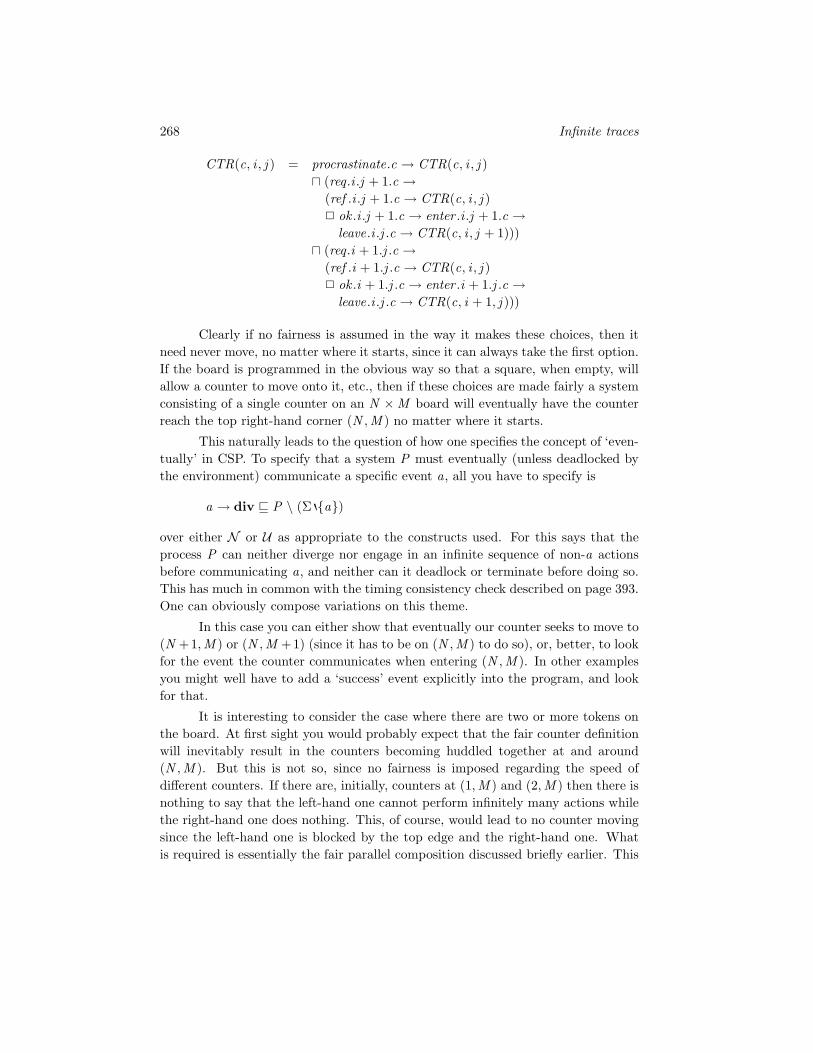
268 Infinite traces
CTR(c, i , j ) = procrastinate.c → CTR(c, i , j ) (req.i .j + 1.c →
(ref .i .j + 1.c → CTR(c, i , j ) ok .i .j + 1.c → enter .i .j + 1.c →
leave.i .j .c → CTR(c, i , j + 1))) (req.i + 1.j .c →
(ref .i + 1.j .c → CTR(c, i , j ) ok .i + 1.j .c → enter .i + 1.j .c →
leave.i .j .c → CTR(c, i + 1, j )))
Clearly if no fairness is assumed in the way it makes these choices, then itneed never move, no matter where it starts, since it can always take the first option.If the board is programmed in the obvious way so that a square, when empty, willallow a counter to move onto it, etc., then if these choices are made fairly a systemconsisting of a single counter on an N ×M board will eventually have the counterreach the top right-hand corner (N ,M ) no matter where it starts.
This naturally leads to the question of how one specifies the concept of ‘even-tually’ in CSP. To specify that a system P must eventually (unless deadlocked bythe environment) communicate a specific event a, all you have to specify is
a → div P \ (Σ a)
over either N or U as appropriate to the constructs used. For this says that theprocess P can neither diverge nor engage in an infinite sequence of non-a actionsbefore communicating a, and neither can it deadlock or terminate before doing so.This has much in common with the timing consistency check described on page 393.One can obviously compose variations on this theme.
In this case you can either show that eventually our counter seeks to move to(N +1,M ) or (N ,M +1) (since it has to be on (N ,M ) to do so), or, better, to lookfor the event the counter communicates when entering (N ,M ). In other examplesyou might well have to add a ‘success’ event explicitly into the program, and lookfor that.
It is interesting to consider the case where there are two or more tokens onthe board. At first sight you would probably expect that the fair counter definitionwill inevitably result in the counters becoming huddled together at and around(N ,M ). But this is not so, since no fairness is imposed regarding the speed ofdifferent counters. If there are, initially, counters at (1,M ) and (2,M ) then there isnothing to say that the left-hand one cannot perform infinitely many actions whilethe right-hand one does nothing. This, of course, would lead to no counter movingsince the left-hand one is blocked by the top edge and the right-hand one. Whatis required is essentially the fair parallel composition discussed briefly earlier. This

10.3 Using infinite traces 269
only makes sense if we remove from the environment the ability to choose whichcounter communicates next. The appropriate way to do this is to place the systemin parallel with a fair arbiter whose job it is to choose which counter acts. If
choices(c) = procrastinate.c, req .i .j .c | i , j ∈ N
then for counters c1 and c2, you can use the arbiter Fair(choices(c1), choices(c2)).(End of example)
Exercise 10.3.1 Complete the programming of the system in the example above bydefining a Square(i , j ) process, any others you need, and putting the complete networktogether.
Exercise 10.3.2 If instead of moving just up and right, the counter chooses fairlybetween trying to move up, down, left and right, need it ever leave the board?
Exercise 10.3.3 The implementation of F given in the text does not work for po-tentially terminating processes. Put this right as follows:
(a) Revise the definition of Fair(A,B) to produce a process TFair(A,B , tk) (for tk ∈Σ (A ∪ B)) whose behaviour is identical except that it is always willing to com-municate tk (as an alternative to its current choice of A or B), upon which itterminates.
(b) In transforming a program with F ’s in, as on page 266, sequentially compose theprevious result with tk → SKIP for some new event tk .
(c) Put together the resulting process with TFair processes, synchronizing appropri-ately, and explain why the result behaves as you would wish.
Exercise 10.3.4 The process Cfin(in, out) can both lose and duplicate messages.Define (in CSP) the most general process Efin(in, out) that acts like a one-place bufferexcept that it can lose any message as long as it does not lose an infinite consecutivesequence of them (i.e., it behaves like Cfin(in, out) except that it never duplicates). Whatrefinement relation, if any, holds between the Cfin(in, out) and Efin(in, out)? Hint: definethe process using F and then use the transformation implementing this.
Exercise 10.3.5 The process
SemiFair(A,B) = RUNA ||| Fair(A,B)
always allows any event in A and need never allow B , but specifically does not permitan infinite trace unless it contains infinitely many events from A. Compute its sets offailures and infinite traces and find a direct definition of this process in the style of thatof Fair(A,B) on page 263.
Construct the process which, for three disjoint sets A, B and C , may at any timeselect between them, and which does not allow infinitely many of either A or B without

270 Infinite traces
the other, and which does not allow infinitely many C without infinitely many each of Aand B .
Exercise 10.3.6 Use a fair arbiter (using the F to introduce it, if you wish) toconstruct the most general finite buffer FinBUFF 〈〉 discussed on page 263.
10.3.2 Fixed-point induction over U
As we saw on page 254, it is not possible to use restriction functions to generatecomplete metrics over models incorporating infinite traces, and indeed constructivefunctions often have multiple fixed points. These facts are as true over U as overI. This is a great pity since the UFP rule and fixed-point induction (whose proofsin Section 9.2 depend on constructiveness and the uniqueness of fixed points) arevery important tools for establishing facts about recursively defined processes.
It is possible to establish weak versions of fixed-point induction and the‘unique’ fixed point rule over U and I. To do this we have to define what a con-structive function is via a family of restriction functions: over U these are defined(F ,D , I ) ↓ n = (F ,D) ↓ n where the restriction on the right-hand side is thatdefined over N , with a similar definition over I. Though these do not generatea metric (there are pairs of distinct processes they cannot separate), we can stilldefine ‘constructive’ and ‘non-destructive’ functions exactly as before, and exactlythe same collections of the standard operators are respectively one or the other (see,for example, Lemma 8.2.3).
While a constructive function over U may not have a unique fixed point, it iseasy to show that all fixed points have identical projections into N . This is becauseyou can inductively prove that if P and Q are two fixed points then P ↓ n = Q ↓ nfor all n. This argument leads to the following result.
Lemma 10.3.1 Suppose F : U → U is constructive, monotonic and has a leastfixed point µF , and P ∈ N (a closed member of U) is such that P U F (P). ThenP U µF
Proof By induction on n it is easy to prove that
P U Fn(P) and Fn(P) ↓ n = (µF ) ↓ n
Suppose b is a finite-length behaviour of µF (i.e., a failure or divergence). Choosingn to be any number greater than its length we thus have that b is a behaviour ofFn(P) and hence of P . Hence
failures⊥(µF ) ⊆ failures⊥(P) (+)
divergences(µF ) ⊆ divergences(P)
10.4 Notes 271
We thus have
infinites(µF ) ⊆ traces⊥(µF ) (1)⊆ traces⊥(P) (2)= Traces(P) (3)
Here, (1) is a consequence of axiom I1, (2) is by (+), and (3) is because of ourassumption that P ∈ N . This implies that
infinites(µF ) ⊆ infinites(P)
completing the proof that P U µF .
This result means that the rule of fixed-point induction (Sections 5.1 and 9.2)is valid over U provided the property you are proving is finitely nondeterministicand the function is constructive.
Of course, both the above lemma and the conclusion regarding fixed-pointinduction extend easily to mutual recursions (i.e., functions in UΛ → UΛ). It alsoleads to the following weak analogue of the UFP rule since under the assumptionsof the following rule we have P U µF by the lemma, but µF is the least fixedpoint.
Unique closed fixed point rule Suppose F : UΛ → UΛ is a constructive, CSPdefinable function, and that P ∈ (N )Λ is such that F (P) = P . Then P = µF .
Thus, if a finitely nondeterministic process satisfies a constructive recursion,it is always the value of the recursion. There are, of course, recursions that do nothave a closed solution like this, an example is µ q .(a → q) ‖
aA∗ which we studied
earlier.
10.4 Notes
The role of infinite traces in modelling unboundedly nondeterministic constructssuch as fairness was well understood before CSP was invented. They were notincorporated into the semantic models for some years, however, because of technicaldifficulties they introduce such as incompleteness and discontinuity.
U was introduced in [105], which also is the main reference for the basicproperties of this model. It proves the existence of fixed points of recursions viaoperational congruence. Barrett’s alternative proof can be found in [5, 7], and isanalyzed further in [84]. Some finer properties of the model can be found in [6, 12].Our understanding of the axioms of U (especially I2) owes much to the work ofStephen Blamey.

272 Infinite traces
2005: The author has now shown [114] that it is possible to build an infinitetraces which is not divergence-strict. A vestige of this strictness remains in thatinfinite traces which are the limits of divergent finite traces are always included.Otherwise it only includes real traces, failures, divergences and infinite traces. Thepenalty for this is an elaborate fixed-point theory.

Chapter 11
Algebraic semantics
11.1 Introduction
Throughout the introductory chapters we used algebraic laws to help explain themeanings of the various operators of CSP. Laws of this type have historically playedan important role in the field of process algebra (the very name of which suggeststhis).
An algebraic semantics for a programming language is one where the notionof process equivalence is derived from a set of laws. Some authors proposing pro-cess algebras have regarded algebraic semantics as the most basic means of definingprocess equality, in that they propose a given set of laws and set about investi-gating what equivalence they produce. The theory most closely associated withthis approach is ACP (see, for example, [9, 10]). This gives a remarkable degree offreedom, since essentially any set of laws will create an equivalence on the set ofprocess terms. There is no constraint on one’s choices that is nearly as sharp as therequirement that a denotational model induce a congruence.
Simply quoting a set of laws does bring the dangers of not identifying pro-cesses that you had intended should be equal, or, more worryingly, identifying far toomany. See Exercises 11.1.1, 11.4.5 and 11.5.3 for examples of the latter. Thereforethe equivalence induced by a proposed set of laws must be thoroughly investigatedto make sure it has the intended effect.
Since we already have a well-established concept of equivalence between CSPprocesses, our approach will be to attempt to characterize that. In other words, wewill attempt to capture the equivalences induced by the various denotational modelsfor CSP described in Chapter 8. Obviously all laws used must be theorems of theequivalence under consideration: if the semantics we are attempting to duplicate is

274 Algebraic semantics
written S[[·]], this just involves proving a series of simple lemmas such as
S[[P Q ]] = S[[Q P ]]
S[[SKIP ; P ]] = S[[P ]]
S[[P ||| (Q ||| R)]] = S[[(P ||| Q) ||| R]]
(in each case for all processes P , Q and R). It is usually not hard to find a largenumber of true laws with respect to a sensible notion of equivalence. Providedall your laws satisfy this basic ‘sanity’ stipulation, and all rules which you use inconjunction with them are valid also, it is plain that they can never prove a pair ofinequivalent processes equal. In the usual logical sense of the word, such a theoryis sound.
The real challenge is in finding, and being able to show you have found,enough laws to be able to prove any pair of equivalent processes equal; in otherwords, creating a complete algebraic theory. This chapter shows how you can dothis. We will deal only with the semantics of finitely nondeterministic CSP withΣ finite. We will also, for now, deal only with the fragment of the CSP languagewithout SKIP or sequential composition since these require special cases that wouldunnecessarily complicate an introductory view of the way algebraic methods work.Most attention is given to the equivalence induced by N , since that is the maindenotational model for finitely nondeterministic CSP.
All the laws given names (e.g., ‘〈hide-dist〉 (3.1)’) in earlier chapters are trueunder all the equivalences generated by the models described in Chapters 8 and 10.Since each of our models equates some pairs of processes that are discriminated inat least one of the others, a set of laws true in all three models cannot be sufficientto capture any one of the model-based equivalences completely, but, as we will see,they require very few additions.
Examples of such pairs of processes are
P = div
P ′ = div ||| a → STOP (equivalent to P in N but not in T )
Q = STOP
Q ′ = STOP div (equivalent to Q in T and F but not in N )
Our existing laws thus cannot prove the equivalences
P =N P ′ and Q =T Q ′
since any such proofs would contradict the inequivalences
Q =N Q ′ and P =T P ′

11.2 Operational semantics via algebra 275
Exercise 11.1.1 A certain text ([53]1) proposes the following laws for CSP (amongstmany others)
(1) P ‖ ⊥ = ⊥(2) P ‖ STOP = STOP
(3) P ‖ Q = Q ‖ P
(4) ⊥ Q = ⊥(5) STOP Q = Q
Which of these are true, and which false, over N on the assumption that ⊥ is identifiedwith div? Show that these laws alone (and hence any superset) are sufficient to provethat P = Q for all processes P and Q .
Exercise 11.1.2 Prove that the following laws are all valid in the semantics of CSPover N :
(a) 〈; -assoc〉 (6.3), (b) 〈hide-step〉 (3.6), (c) 〈hide-combine〉 (3.3).
11.2 Operational semantics via algebra
An operational semantics does not have to follow the pattern set out in Chapter7: all we require is a formally-based method of implementing a language. You cando this via systematic algebraic transformations: a reduction strategy very muchlike those used for functional programming. A way of implementing CSP in thisfashion is to calculate the selections of initial actions a process can communicate bytransformation to a process of the form2
N
i=1?x : Ai → Pi
where, of course, the Pi are terms that can depend on the identifier x . By anal-ogy with functional programming, an appropriate name for this is head normalform (hnf)3. To execute a process, you thus transform it into this form and make
1An amazing proportion of the ‘laws’ stated in [53] are false, and it is possible to find manydistinct combinations which prove all processes equal. Three disjoint such sets can be found inthis exercise and Exercises 11.4.5 and 11.5.3 in this chapter. Some of the laws given in that bookmake even less sense than simply being false: for example ‘P ||| Q ∧ Q ||| R ⇒ P ||| R’ which istrivially ill-typed since processes are not truth values.
2Here, N
i=1Qi is an abbreviation for Q1 (Q2 . . . (QN−1 QN ) . . .), though in what
follows we will not go explicitly through the transformations required to turn more arbitrarilyconstructed nondeterministic compositions into this precise, right-associated, form. This can, ofcourse, be done with the laws 〈-assoc〉 (1.6), 〈-sym〉 (1.4) and 〈-idem〉 (1.2) in such a way asto guarantee that all the Qi are different.
3The formal definition of hnf will appear on page 280 and be a little more general than this.

276 Algebraic semantics
an arbitrary selection from the nondeterministic choice of initial selections Ai ofactions which are thereby displayed. If the environment picks one of these, it iscommunicated and we can repeat the procedure on the result process, and so on.
There are four types of laws required to do this:
• the distributive laws, for removing nondeterministic choices to the outside;
• the step laws, which calculate the first-step actions of constructs like P ⊕Qin terms of those of P and Q ;
• the unwinding law of recursion; and
• manipulations of the expressions within processes.
Just as in earlier chapters we have avoided going into details about the syntaxand semantic details of sub-process expressions, here we will generally assume thatone of these can always be replaced by an equivalent expression without comment.The only law as such we will need is one to change the names of input identifiers:
?x : A→ P = ?y : A→ P [y/x ]if y is not free in P
〈input α-cnv〉 (11.1)
While this is frequently needed to perform the transformations below, in describingthem we will simply assume it has been used to unify the names of inputs wherenecessary without further comment.
The strategy for reducing an arbitrary process P into hnf is quite simple,and is as follows:
• If P has the form ?x : A→ P ′, it is already in the required form so we needdo nothing.
• If P has the form P ′ P ′′, then reduce each of P ′ and P ′′. The resultingprocess (P ′
1 P ′′1 , say) is in the required form.
• If P is STOP , then apply the law 〈STOP -step〉 (1.15).
• If P has the form P ′ ⊕ P ′′, where ⊕ is any other standard binary operator(i.e., , ‖
X, ||| or X ‖Y ), then first reduce each of P ′ and P ′′, to P† and P‡,
say. Next, use the left and right distributive laws of ⊕ (in each case the rightdistributive law is proved using the left distributive law and the symmetrylaw) to move all the top-level nondeterminism from P† and P‡ to the outside.The result then has the form
N
i=1(?x : Ai → P†
i )⊕ (?x : Bi → P‡i )

11.2 Operational semantics via algebra 277
In each case the respective step law (〈-step〉 (1.14), 〈‖X
-step〉 (2.10), 〈|||-step〉(2.6) or 〈X ‖Y -step〉 (2.2)) transforms this into the required form.
• If P has the form P ′[[R]], then very much the same procedure (using 〈[[R]]-dist〉(3.13) and 〈[[R]]-step〉 (3.15)) is followed.
• If P has the form P ′ \ X , then applying the same procedure (using 〈hide-dist〉(3.1) and 〈hide-step〉 (3.6)) will result in a process of the formN
i=1Qi where
the Qi either have the form ?x : Ai → (Q ′i \ X ), which is what we want, or
(?x : Ai → (Q ′i \ X )) P ′′
i,j \ X | j ∈ 1, . . . ,Mi
which is not. The second case occurs, evidently, when some of the initialactions of P ′ are hidden and so do not create initial visible actions of P (inthe operational semantics of Chapter 7 they would have become τ ’s).The strategy in the second case is to reduce the processes P ′′
i,j \ X , and thenuse the definition of P Q = (P Q) Q and 〈-step〉 (1.14) to organizethe result into the correct shape. (*)
• If P is recursively defined, simply apply 〈µ-unwind〉 (1.23) and reduce theresult. (**)
There is a significant problem with this strategy, namely it need not termi-nate. The problem is that the clauses for reducing P \ X and µ p.P can both resultin infinite regression: the reduction-based operational semantics diverges ratherthan produces a term of the required form. In fact, this is just as well, becauseof course there are CSP terms in the language we are considering that are notequivalent in N to any process in head normal form: the ones that can divergeimmediately.
The reduction strategy must therefore certainly fail on any term mapped bythe semantics to ⊥N . This can easily be demonstrated on divergent terms such as
(µ p.a → p) \ a µ p.p µ p.STOP p
The converse (i.e., the strategy succeeds on any other term) is also true, because itis easy to show that any infinite regression contains an infinite number of uses of (*)and (**), the application of either of which generates a τ in the original operationalsemantics.
Example 11.2.1 Consider the process (COPY ||| COPY ) \ | left |. To trans-form this to hnf we first expand the two recursions: this immediately brings eachof them into the hnf
left?x → right !x → COPY

278 Algebraic semantics
The law 〈|||-step〉 (2.6) then brings the interleaving to the hnf
left?x → ( (right !x → COPY ) |||(left?x → right !x → COPY ))
left?x → ( (left?x → right !x → COPY ) |||(right !x → COPY ))
which (thanks to 〈|||-sym〉 (2.7) and 〈-idem〉 (1.2) and re-folding the recursion)can be simplified to the hnf
left?x → ((right !x → COPY ) ||| COPY )
(Such simplifications are not a necessary part of the procedure, but help.)
We then apply 〈hide-step〉 to this to transform the complete process (incor-porating the external hiding) to
((right !x → COPY ) ||| COPY ) \ | left | | x ∈ T
This, of course, is not in hnf since the hiding takes away the visible guard. Wetherefore have to re-apply our strategy to the processes
((right !x → COPY ) ||| COPY ) \ | left | (§)
which yields
right !x → (COPY ||| COPY ) left?y → ((right !x → COPY ) ||| (right !y → COPY ))
for the process inside the hiding. (Bear in mind that in practice it is a lot clearerto use an appropriate mixture of prefix choices such as left?y and external choicesof these to represent a given initial set of actions of a given branch of an hnf, ratherthan using the pure prefix-choice form used in the definition, though the latter couldeasily be recovered using 〈-step〉 (1.14).) Thus (via 〈hide-step〉 again) the process(§) becomes
right !x → (COPY ||| COPY ) \ | left | ((right !x → COPY ) ||| (right !y → COPY )) \ | left | | y ∈ T
This is still not hnf, since we have once again lost some of the guards to thehiding. We now have to re-apply our strategy once more to
((right !x → COPY ) ||| (right !y → COPY )) \ | left |

11.3 The laws of ⊥N 279
which fortunately does now yield an hnf:
right !x → (COPY ||| (right !y → COPY )) \ | left | right !y → ((right !x → COPY ) ||| COPY ) \ | left |
(It would really be purer to separate the cases of x = y and x = y as would be doneby 〈-dist〉, but it would be even more complex!) We can now collect together anhnf for (§): after a little manipulation it is
right !x → (COPY ||| COPY ) \ | left | (COPY ||| right !y → COPY )) \ | left |
right !y → (right !x → COPY ||| COPY )) \ | left || y ∈ T
and the hnf for the original process is then just the nondeterministic choice overthis as x varies.
Obviously if we had hidden | left | in a buffer with no initial bound on howmany inputs it can take, such as BUFF 〈〉, then the strategy would not terminate.(End of example)
Exercise 11.2.1 Reduce the following processes to hnf:
(a) COPY \ | right |(b) ((a → Pa) (b → Pb)) ||| ((b → Qb) (c → Qc))
(c) COPY \ left .0 where the type T of the channels is 0, 1
11.3 The laws of ⊥N
Our attempts to reduce divergent processes to hnf failed in the previous sectionbecause the divergence translated itself into non-termination of the reduction algo-rithm. It is a good idea to include an explicit representation of a divergent processin the language we reason about algebraically: let div represent this as it did inSection 3.1. We can then see how a term that is equivalent to a diverging processbehaves algebraically.
As one might expect from the discussions in Chapter 8, it is in the handling ofdiv that N differs from the models without an explicit representation of divergence(F and T ). The laws for div (equalling ⊥N ) over N are thus often not validover these other models: with the exception of prefixing and the right-hand side ofsequencing, all operators are strict (in the sense defined on page 496). Notice thatthe names of these laws reflect their selective validity. They are called zero lawsbecause of their similarity to the arithmetic equivalence 0× x = 0.
div P = div 〈-zeroN 〉 (11.2)

280 Algebraic semantics
div P = div 〈-zeroN 〉 (11.3)
div ‖X
P = div 〈‖X
-zeroN 〉 (11.4)
div X ‖Y P = div 〈X ‖Y -zeroN 〉 (11.5)
div ||| P = div 〈|||-zeroN 〉 (11.6)
div \ X = div 〈hide-zero〉 (11.7)
div[[R]] = div 〈[[R]]-zero〉 (11.8)
div; P = div 〈; -zero-l〉 (11.9)
These laws mean it makes sense to add the term div as an alternative headnormal form: we can now formally define a process to be in hnf if
• it is div, or
• it has the form ?x : A→ P , or
• it is N
i=1Qi for processes Qi in hnf.
The laws mean that if either div appears explicitly in a program or youcan recognize and replace4 some divergent term by it, then you can extend thereduction strategy to deal with this. Essentially, if div is encountered at any levelin reducing a process P to calculate its initial behaviour, then these laws (togetherwith symmetry laws to derive the right-zero laws for binary operators other than ;)will reduce the process itself to div.
The definition of hnf above makes it optional whether to reduce a process inwhich div appears as a choice, such as
(?x : A→ P) div
to div using 〈-zeroN 〉. For simplicity, let us assume that we always do make thisreduction.
4If the replacement is going to form part of our algebraic semantics, then it is clear thatthe means of performing it would have to be formalized, justified, and incorporated within thesemantics.

11.4 Normalizing 281
The possible outcomes of the reduction strategy are then (i) the originaltype of hnf, (ii) the term div and (iii) non-termination of the strategy. There isno complete algorithm for telling if a given CSP term diverges5 or not, and so noeffective procedure which will tell us which terms our strategy will fail to terminateon.
There is a simple and powerful6 algebraically-based method for detectingdivergence, namely:
LoopN If, during an attempt to reduce a process P to head normal form the (syn-tactic) process P is encountered other than at the root of the reduction,then P is divergent and may be replaced by div.
This is not, of course, a law in the conventional sense of the word, rather arule. To implement this rule it is necessary to keep a record of the tree structurethat results from the attempt to reduce a process, and look for loops (nodes identicalto predecessors). The notation LoopN indicates that this is a valid rule over N ,but not over T or F .
11.4 Normalizing
It is our objective to be able to prove any pair of equivalent processes equal usingan algebraic theory. An obvious approach to this is to identify a normal form: ahighly restricted syntax for processes meeting the following requirements.
• A pair of normal form programs are only semantically equal if they are eithersyntactically identical, or perhaps differ in a well-defined and trivial way suchas the name of a bound variable or the order of terms composed under asymmetric and associative operator.
• Every program is equivalent to one in normal form.
• This equivalence can be demonstrated by the algebraic theory.
Let us restrict ourselves, for the time being, to processes that are finitelytransformable to hnf, as are all successors reached when executing their algebraicoperational semantics. (In other words, processes in which all divergences are eithersyntactically explicit, div, or detectable using a rule such as LoopN .)
5This would solve the halting problem.6Inevitably, given the previous discussion, it is not complete in the sense of detecting all di-
vergence. It is, however, complete provided the process is finite state. It then corresponds to adepth-first search for loops in the graph of nodes reachable from the chosen root.

282 Algebraic semantics
Our approach will be to refine the concept of head normal form into a fullnormal form, and to show how a program in head normal form can be transformedusing the laws of and into this restricted form.
Given that Σ is finite, the first-step behaviour P ↓ 1 of any process P iscompletely characterized by the following information:
• Does P diverge immediately? If not,
• what is P ’s set of initial actions initials(P), and
• what are P ’s maximal refusals?
The divergent case of head normal form evidently captures the first of these precisely,but the non-divergent one is too loose in that there are typically many different setsA1, . . . ,AN of initial actions that would give rise, in
N
i=1x : Ai → Pi
to exactly the same sets of initial actions and maximal refusals, bearing in mindthat the complements of the Ai are the refusals. For example,
a, b, c, a, bb, c, a, ba, b, c, a, b, a, ba, b, c, a, b, a, c, b, c, a, b
all give the same result, and are by no means the only sets that give this particularone. We need to decide on a unique representation of any given collection of accep-tance sets7 Ai and provide a way of transforming any non-div head normal formto this. There are various sensible choices one could make, but the one we opt forhere is to specify that the set A1, . . . ,AN
7The concept of an acceptance set is obviously very closely related to that of a refusal set. If wedefine an acceptance set just to be the complement of a refusal set (in Σ) then clearly we couldhave replaced all uses of refusal sets in our models with them, subject to systematic changes indefinitions. This would, however, imply that acceptance sets were superset-closed (as an analogyto axiom F2), implying there were members of ‘acceptance sets’ that a process could never accept.Thus an acceptance is arguably better defined to be a set of events which is (a) the complement ofsome refusal and (b) contained in initials(P). This modification means that the translation fromrefusal sets to acceptance sets is not so direct and means that model, operator, etc. definitionswork better with failures rather than with their acceptance-set analogues. So it seems that inorder to create acceptance-based analogues of the models N and F one either has to compromiseon naturalness or on ease of manipulation. Perhaps the most natural acceptance-set model is thatproposed in [87], which has no superset closure condition at all: modulo divergence, an acceptanceset is the set of all events offered by some stable state. This gives a subtly different (and lessabstract) congruence which fails the law 〈--dist〉 (1.13).

11.4 Normalizing 283
• has the property that A1 ⊃ Aj for all j > 1 (i.e., A1 is the union of all Ai
and represents initials(P)), and
• if i , j > 1 are distinct then Ai ⊆ Aj (i.e., all these Ai represent minimalacceptances, and hence their complements, the maximal refusals).
Note that in the case where initials(P) is a (necessarily the only) minimal accep-tance, N = 1 and A1 plays a double role.
A simple procedure, which is described below, transforms an arbitrary non-div head normal form to this format. It rests almost entirely on the laws of , ,prefixing and conditionals.
You can ensure that each set Ai only appears once in the result by applyingthe law 〈input-dist〉 (1.11) repeatedly till all pairs of identical ones are eliminated.
If there is only one Ai remaining after this, there is nothing further to do. Ifthere are more than one, we have to ensure the collection contains the union andthat all the rest are minimal. Observe that, for any processes P and Q ,
P Q = (P Q) (P Q)by 〈-idem〉 (1.1)
= (P Q) P Qby 〈-dist〉 (1.7), 〈-idem〉 (1.2), etc.
This argument can (see Exercise 11.4.1) be extended, by induction, to show thatfor any N and processes Qi ,
N
i=1Qi = (
N
i=1Qi) (N
i=1Qi)
In the case where Qi =?x : Ai → Pi , the extra process Q1 . . . QN can betransformed using 〈-step〉 (1.14) to the form
?x : A† → R
where A† =⋃N
i=1 Ai and such that, for any a ∈ Aj , we have
Pj [a/x ] R[a/x ] = R[a/x ]
Any a ∈ A† may appear in several different Ai , and the processes Pi [a/x ],which are the possible results of performing it, may all be different from each otherand R[a/x ]. What the above does ensure is that R[a/x ] is the most nondeterministic
284 Algebraic semantics
of these choices. Consider the transformation:
(?x : A† → R) (?x : Ai → Pi)
=(?x : A† Ai → R ?x : Ai → R) (?x : Ai → Pi)
by 〈-step〉 and 〈<I ·>I -idem〉 (1.17)
= (?x : A† Ai → R ?x : Ai → Pi) (?x : Ai → R ?x : Ai → Pi)by 〈--dist〉 (1.13)
= (?x : A† Ai → R ?x : Ai → Pi) (?x : Ai → (R Pi))by 〈input-dist〉 (1.11)
= (?x : A† Ai → R ?x : Ai → Pi) (?x : Ai → R)by what we established about R above
= (?x : A† Ai → R ?x : Ai → R) (?x : Ai → Pi ?x : Ai → R)by 〈-dist〉
= (?x : A† → R) (?x : Ai → Pi R)by 〈-step〉, etc.
= (?x : A† → R) (?x : Ai → R)by what we established about R above
What this does is to show we can replace all the old result processes Pi by R in theprocess we are transforming, making all the possible results of performing a given aidentical. This is both a vital part of the normalization process itself and is helpfulfor the next and final part of transforming it to our target shape of hnf, which is theremoval of any non-minimal Ai (other than A†). This makes use of the followingidentity, which is essentially that proved in the last part of Exercise 3.1.5.
(P Q S ) P = (P Q S ) (P Q) P
since we can then, for any Ai ⊂ Aj , set
P = ?x : Ai → RQ = ?x : Aj Ai → RS = ?x : A† Aj → R
and apply the identity from right to left.

11.4 Normalizing 285
What we have managed to do is transform our process P into a one-stepnormal form: a hnf which is either div or satisfies the restrictions on its acceptance-set pattern set out above and furthermore has a unique successor process for eachinitial action. This gives a complete characterization of the first-step behaviourof the original process P , and has the property that (provided P does not equaldiv) for each a ∈ initials(P) we have P/〈a〉 = R[a/x ]. If P ′ were another processequivalent to P in N then it would reduce to a one-step normal form with exactlythe same shape (pattern of Ai , except that the Ai for i > 1 may be re-ordered)and such that its successor process R′ is equivalent to R in N (in the sense thatR[a/x ] = R′[a/x ] for all a in the initials set A†).
This notion of a one-step normal form extends naturally to a full normalform: the definition is exactly the same except that, in addition, we insist that eachof the result processes R[a/x ] is also in normal form. (It is in doing these lower-level normalizations of the leaf processes of a one-step normal form that we need theassumption that all successor processes can be reduced to hnf.) The argument inthe previous paragraph can easily be extended by induction to show that any pairof normal form programs which are equivalent in N have equivalent normal formstructures and can trivially be inter-transformed by laws. The only things that candiffer are things like the order of Ai ’s and the names of input variables.
It would seem that we have attained our goal of completely capturing thedenotational equivalence via algebra. Essentially we have, but not as simply asit appears on the surface. The problem is how to handle processes that can goon communicating for ever and which therefore fail to have a finite-depth normalform. It is evident that we can attempt fully to normalize a process P by firsttransforming it to one-step normal form and then normalizing each of the resultprocesses R[a/x ], but this transformation will only terminate and produce a finite-depth normal form program if the set traces⊥(P) divergences(P) is finite (which,under our assumptions, is equivalent to there being a bound on the length of itsmembers). There are several ways around this difficulty, but all mean we have toabandon any hope that all pairs of equivalent CSP processes are inter-transformableby a finite sequence of law applications.
The first approach we can take is to incorporate into our theory the fact thatprocesses P and Q are equivalent in N if, and only if, P ↓ n = Q ↓ n for all n ∈ N,where the restriction functions ↓ n are as defined on page 200. We can expressP ↓ n directly in CSP8, it is P ‖
ΣRest(n) where
Rest(0) = divRest(n) = ?x : Σ→ Rest(n − 1) for n > 0
8The expression given here is dependent on our assumption that P never terminates. For howto extend this idea to processes that can communicate , see Exercise 11.5.4.

286 Algebraic semantics
Since each P ↓ n always has a finite normal form, the rule
EquivN If P and Q are any processes in finitely nondeterministic CSP, definedwithout SKIP or sequential composition, then they are equivalent in Nif and only if, for all n ∈ N,
P ‖Σ
Rest(n) = Q ‖Σ
Rest(n)
leads directly to a decision procedure for equivalence which involves convertinginfinitely many processes into finite normal form and seeing if you get the sameresults for each pair. It is complete on processes satisfying our assumptions aboutreducibility to hnf.
Another approach is to transform the program into a potentially infinitenormal form tree. It is perhaps easiest to understand this in terms of deriving,from a process P , a recursive definition of a vector of processes which turns outto be indexed by T , the set of members of traces⊥(P) other than non-minimaldivergences. If s is such a trace, we can compute Rs , the result process (equivalentto P/s) derived from applying the one-step normal form transformation down s asfollows.
R〈〉 = PRs 〈a〉 = Q [a/x ], where applying the one-step normal form trans-
formation to Rs yields something of the form
N
i=1?x : Ai → Q
Along with this derivation you have produced an expression for each Rs in termsof the Rs 〈a〉: the one-step normal form of Rs . If you now replace the processesRs by the corresponding components of a vector N of process variables, the resultis a constructive one-step tail recursion whose unique fixed point in NT is clearly〈Rs | s ∈ T 〉 = 〈P/s | s ∈ T 〉. If P ′ is a process equivalent to P then the recursionproduced will be exactly the same, since the one-step normal form of P ′/s has thesame shape as that of P/s for all s . So we have managed to transform P and P ′ tothe same process definition, albeit using in many cases an infinite number of steps.
When deriving this ‘tree’ expression for the normal form, it may very wellbe the case that the number of distinct values of P/s visited is actually finite. Thisis always so if P is finite state and even sometimes when it is not, for example
µ p.a → (p ||| p) (equivalent to µ p.a → p)
If you can recognize these equivalences (by transformation, for example), then youcan produce a more compact representation of the normal form tree as a finite graph

11.4 Normalizing 287
or as a recursion with a finite indexing set. Thus you can represent the process
P0 = µ p.(a → a → p) (a → STOP)
as the two-state recursion
N〈〉 = a → N〈a〉
N〈a〉 = a → N〈〉 STOP
rather than having a component for each member of a∗.The problem with this is that it re-introduces an element of flexibility into
the way normal form processes are structured: flexibility is just what you do notwant of a normal form. The main source of flexibility is the fact that one may ormay not spot an equivalence between a pair of processes. Consider, for example,the process
P1 = P0 ‖a,b
(µ p.a → a → ((a → p) (b → STOP)))
This is, in fact, equivalent to P0, but the finite-state normal form you would bemost likely to derive for it is
N ′〈〉 = a → N ′
〈a〉
N ′〈a〉 = a → N ′
〈a,a〉 STOP
N ′〈a,a〉 = a → N ′
〈a,a,a〉
N ′〈a,a,a〉 = a → N ′
〈a,a,a,a〉 STOP
N ′〈a,a,a,a〉 = a → N ′
〈a,a,a,a,a〉
N ′〈a,a,a,a,a〉 = a → N ′
〈〉 STOP
because the structures of, for example, P1/〈〉 and P1/〈a, a〉 are sufficiently differentthat it is unlikely one would spot or easily prove their equality while transformingto normal form.
If the above were computed for P1, then one can no longer establish its equiv-alence with P0 by the identity of their normal forms. The way around this, though it
288 Algebraic semantics
is not in any obvious sense an algebraic operation, is to factor each normal form youcompute by the maximal bisimulation computed over it9 (see Section 7.2). In thecase above this identifies N ′
〈〉,N′〈a,a〉,N
′〈a,a,a,a〉 and N ′
〈a〉,N′〈a,a,a〉,N
′〈a,a,a,a,a〉
resulting in a structure identical to the normal form of P0 (which has no interestingequivalences between its nodes).
These bisimulated normal forms are in some ways less attractive from apurely algebraic standpoint than the ones with separate components for all traces,but they are a lot more practical since they are so often finite. Though they arederived via direct manipulation of the underlying LTS rather than by algebraictransformations, the normal forms which play a crucial part in FDR’s operationsare essentially the same objects. See Appendix C for more details.
The reader might have noticed the great similarity between the normal formsdescribed in this section and the recursion defined on page 235 to demonstrate thecoverage of N by the CSP notation. This should not come as a surprise, since ineach case our task was to find a standard way of representing a given semanticvalue, even if we did have to approach this problem from opposite ends. Exceptfor the fact that we have, in this chapter, yet to deal with SKIP and sequencing,the only difference between the recursions Ns defined above and IntN
(F ,D) definedon page 235 is the indexing sets used. In the second case this is, for a given value(F ,D) ∈ N ,
(F ,D)/s | s ∈ T
where T is, again, the set of traces other than non-minimal divergences. Naturally,in comparing this with the normal form of a process P such that
(F ,D) = (failures⊥(P), divergences(P)) = SN [[P ]]
it is not hard to prove that the relation over T defined
s ≡ s ′ ⇔ SN [[P ]]/s = SN [[P ]]/s ′
corresponds precisely to the maximal bisimulation over the processes Ns derivedfrom P . This demonstrates nicely that the result of quotienting the maximal bisim-
9This bisimulation can be computed in two ways. The first is to use the ordinary bisimulationrelation over the LTS you get from the standard operational semantics of the normal form recursion.Before bisimulating you would then start with distinct nodes for all the normal form states, andalso extra states (reachable under τ actions from this first sort) for the initials sets and maximalrefusals. The second, and much more elegant, way is to consider only the normal form states asnodes of the transition system. The nodes are marked with divergence or with maximal refusalinformation which is taken into account when computing the maximal bisimulation: no two nodeswith different markings are ever identified. See Section C.2 for more discussion of this idea.
11.4 Normalizing 289
ulation into any ‘normal form’ of the sort represented by the N ′s above gives a true
normal form. In other words, it demonstrates the ‘completeness’ of the method.
To summarize, we have shown that the algebraic laws completely characterizethe semantics of CSP over N , though the procedures we have provided for decidingequivalence are infinitary. The only remaining issue is our assumption that we candetect all divergent terms and replace them with div. The procedure for reducing aprocess to hnf does, of course, provide an infinitary complete method for this, and wecould argue reasonably that if we are to accept an infinitary procedure for one thingthen it will do for this too! The unfortunate feature is that it leads to one infinitaryprocedure (divergence detection) being a frequently-used subroutine in another.You can get round this (i.e., back to a single level of infinity) by several methods,perhaps the most frequently used of which is the concept of syntactic approximationwhere, instead of comparing the desired pair of processes algebraically, you comparepairs of recursion-free approximations (where recursions have been unwound a finitenumber of times, and those that remain are replaced by div). For more details ofthis, see [45], for example.
It is well worth commenting that the normalization procedure uses a sur-prisingly small proportion of the laws set out in earlier chapters. The laws ofprefixing and choice have been used extensively in normalization, but the only lawsused for other operators have been unwinding and their distributive, step and zero(strictness) laws (with the exception that some symmetry laws are needed to derivesymmetric versions, such as right distributive laws from left ones). The only possibleconclusion is that the rest of the laws must be implied by the ones we used, ex-amples being 〈|||-assoc〉 (2.8), 〈X ‖Y -assoc〉 (2.5), 〈hide-‖
X-dist〉 (3.8), 〈hide-combine〉
(3.3) and 〈f [·]-‖X
-dist〉 (3.9). None of these is a trivial consequence of the ones we
used in the same sense that 〈hide-sym〉 follows from 〈hide-combine〉. It is usuallypossible to prove them from the algebraic theory, but the proofs are generally muchharder than those directly using the underlying models. The proofs often make useof the rule EquivN and inductions such as
((P ||| Q) ||| R) ↓ n = (P ||| (Q ||| R)) ↓ n
in which, for the inductive step, the two sides are reduced to hnf. See Exercise11.4.2.
Algebraic semantics also give us (as discussed earlier) the freedom to ask thequestion of what equivalence is induced if we drop one or more of the laws thatactually were necessary to characterize failures/divergences equivalence. The mostinteresting ones to consider dropping are 〈--dist〉 (1.13), which plays a crucial rolein normalization and which is, as discussed at the point of its definition on page32, somewhat hard to justify on intuitive grounds, and the step laws of parallel

290 Algebraic semantics
operators. But all of this is beyond the scope of this text, and in any case theoccupation of experimenting with sets of laws for its own sake is a great deal morefascinating theoretically than it is practically useful.
Exercise 11.4.1 Prove, using the laws and induction on N , that for any P1, . . . , PN
N
i=1Pi = (
N
i=1Pi) (N
i=1Pi)
Exercise 11.4.2 Using the expression for P ↓ n given in the statement of the ruleEquivN , show by induction on n that for any processes P , Q and R
((P ||| Q) ||| R) ↓ n = (P ||| (Q ||| R)) ↓ n
by computing the hnf’s of the right- and left-hand sides in terms of hnf’s of P , Q and R. Doyou think this form of induction would work as easily for proving the law 〈hide-combine〉?
Exercise 11.4.3 Compute finitely mutual recursive normal forms for (COPY |||COPY ) \ | left |, dealt with in Example 11.2.1 and the process of Exercise 11.2.1part (c).
Exercise 11.4.4 Recall the interrupt operator described on page 239. P a Qbehaves like P except that at any time a may occur and the process subsequently behavelike Q . Give the failures/divergences semantics of P a Q . Is it strict in P? and in Q?
Now give a step law that allows the reduction strategy to hnf to be extendedto processes involving a constructs together with the strictness properties above anddistributive laws.
Notice that these laws completely determine the semantics of this new operator.Do you think a similar principle applies to any new operator?
Exercise 11.4.5 Repeat Exercise 11.1.1 for the following ‘laws’ (also taken from [53]),though this time only showing all divergence-free processes equal.
(1) P ‖ RUN = P
(2) P STOP = P
(3) P Q = Q P
(4) P ||| STOP = P
(5) P ||| RUN = RUN ⇔ divergences(P) =

11.5 Sequential composition and SKIP 291
11.5 Sequential composition and SKIP
We have not dealt with SKIP , and hence sequential composition, so far becauseit necessarily adds cases to the reduction/normalization strategies and to the def-initions of the normal forms. This is not only because we are not permitted toinclude in choice sets Ai but also because is, as seen in earlier chapters, nottreated like other actions. The law 〈-SKIP resolve〉 (6.6) was crucial in explainingthe difference earlier, and it has a large impact on how the algebraic semantics areaffected by .
The crux of the problem is that we now have processes like (a → STOP)
SKIP which can offer an event in Σ transiently before they terminate. In manyways the behaviour of this process is similar to
((a → STOP) (b → c → STOP)) \ b
in that both can independently make the decision to remove the choice of doing ain favour of something else. This latter process has hnf (indeed, normal form)
(?x : a, c → STOP) c → STOP
In other words, the process with the transient event a has been replaced by a processdefinition without transients which has identical observed behaviour. This is notpossible with the first process, because it involves the trick of offering the externalchoice of the transient a and the result of the internal choice, and we do not permitprocess definitions like
(?x : a, → STOP) SKIP
which would be the translation.
There are two reasonable ways to incorporate termination into hnf. In someways the more pleasing is to bring the sliding choice/timeout operator P Q intothe syntax of hnf, thinking of it as a primitive operator implemented as in the directoperational semantics for it on page 169 rather than as (P Q) Q (thoughthe equality over denotational models with this representation would still hold).However, because some people might find this ‘doublethink’ about confusing,and because it is probably simpler overall, we will add termination by allowing(?x : A→ P) SKIP to be considered an hnf.
The definition of hnf now becomes:
• div is in hnf;
• SKIP is in hnf;

292 Algebraic semantics
• ?x : A→ P is in hnf;
• (?x : A→ P) SKIP is in hnf;
• if each Qi is a hnf, then N
i=1Qi is;
When we want to distinguish this extended form we will refer to it as -hnf.
The idea that reducing to hnf provides an operational semantics easily ex-tends to this larger class. Obviously SKIP terminates, whereas (?x : A→ P) SKIPmay offer the choice of A for a short time before terminating.
Imagine you are reducing a construct like P⊕Q (⊕ being any binary operatorother than or, with the obvious modifications, renaming or hiding) to -hnf. Therecipe given earlier calls for us first to reduce P and Q . Clearly you need to dealwith the extra cases that arise when one or both of the results, P ′ and Q ′, areof the form SKIP or (?x : A → R) SKIP . The laws of SKIP given in Section6.3 easily deal with all combinations of SKIP with itself and prefix choices. AndSKIP ; Q ′ and ((?x : A → P) SKIP); Q ′ reduce, for any Q ′, via 〈; -unit-l〉 (6.4)and 〈; -step〉 (6.7).
The remaining cases for can be dealt with using existing laws, and the caseof ((?x : A → P) SKIP)[[R]] by 〈[[R]]--dist〉 (3.14) and 〈SKIP-[[R]]-Id〉 (6.10).The corresponding case for \ X requires a new law which is closely based on itsexisting step law:
((?x : A→ P) SKIP) \ X =
(?x : A→ (P \ X )) SKIP<I A ∩ X = >I
((?x : A X → (P \ X )) SKIP P [a/x ] \ X | a ∈ A ∩X
〈hide-SKIP-step〉 (11.10)
Parallel operators require three new laws each: one each for an input/SKIP com-bination in parallel with a different type of -hnf. (There is no need to introducea law to deal with the cases where the other process is a nondeterministic choice ordiv since these are reducible by distributive and zero laws respectively.) Becauseof this multiplicity we only give those for ‖
X, since each of ||| and X ‖Y are express-
ible in terms of it. The second and third of these are better and more succinctlyexpressed as general principles involving the construction (bearing in mind thelaw 〈-SKIP resolve〉). These laws make it straightforward to extend the strat-egy so that it can reduce CSP processes possibly involving SKIP and sequential

11.5 Sequential composition and SKIP 293
composition to -hnf.
((?x : A→ P) SKIP) ‖X
SKIP =
(?x : A X → (P ‖X
SKIP)) SKIP〈‖X
- SKIP〉 (11.11)
(P Q) ‖X
(R S ) =
(P ‖X
R) ((Q ‖X
(R S )) ((P Q) ‖X
S ))〈‖X
--split〉 (11.12)
(P Q) ‖X
(?x : A→ R)) =
?x : A X → ((P Q) ‖X
R)
((P ‖X
?x : A→ R) (Q ‖X
?x : A→ R))
if x is not free in P or Q
〈‖X
--input〉 (11.13)
Given its similarity to the normal form in the SKIP -free case, it is naturalto look to the full abstraction recursion on page 235 for guidance about how toextend the definitions of one-step and full normal forms. The first-step behaviourof any non-divergent process is now characterized by its initial actions (which maynow include ) and the minimal acceptance sets which are subsets of Σ. Minorextensions to the strategy given in the previous section can transform any -hnf toone of the following forms:
(a) div
(b) ?x : A→ R
(c) (?x : A→ R) SKIP
(d) (?x : A → R) (N
i=1?x : Ai → R) where the Ai are incomparable proper
subsets of A
(e) ((?x : A→ R) SKIP) (N
i=1?x : Ai → R) where the Ai are incompara-
ble subsets (not necessarily proper subsets) of A.
Here, (a) is the representation of a divergent process, (b) of a process which cannotterminate or behave nondeterministically on its first step and (c) of a process whichcan terminate immediately and must do so if no member of A is accepted quicklyenough. (d) and (e) add the possibilities of nondeterministic offers of proper subsetsof the initials to the cases in (b) and (c).

294 Algebraic semantics
The most important new transformation required to bring the manipulationof an arbitrary -hnf to one of these forms is developed in Exercise 11.5.1 below.
The above is the extended definition of one-step normal form, and the methodsand problems associated with converting this to a full normal form are exactly asfor the smaller language in the previous section.
Exercise 11.5.1 Show algebraically that for any P and Q ,
(P SKIP) (Q SKIP) = (P Q SKIP)
Why is this useful for transforming a -hnf process to one-step normal form?
Exercise 11.5.2 Our dealings with the combinations involving P SKIP and paralleloperators would have been simplified if the distributive law
(P Q) ‖X
R = (P ‖X
R) (Q ‖X
R)
were true. Give an example to show that it is not.
Exercise 11.5.3 Repeat Exercises 11.1.1 and 11.4.5 for the following ‘laws’ (also takenfrom [53]), proving all processes equal.
(1) STOP ; P = STOP
(2) P ; STOP = P
(3) SKIP ; P = P
(4) P ; (Q ; R) = (P ; Q); R
It can be done with, or without, the associative law (4), which is, of course, true.
Exercise 11.5.4 Recall that on page 285 we showed how to define restriction overN for -free processes via a process context. Assuming that there is some event a ∈ Σthat P never communicates on a non-divergent trace, find a corresponding way of definingP ↓ n when P can terminate.
Hint: consider P ; (a → SKIP) in parallel with a well-chosen process.
11.6 Other models
We will not deal with the algebraic characterization of the other models for finitelynondeterministic CSP in as much detail, since many of the basic principles are thesame and, as we will see, in some ways the algebraic approach does not work quiteas cleanly for T and F as for N .

11.6 Other models 295
Over both F and T we have the law
P div = P 〈-unitT ,F 〉 (11.14)
which is, of course, radically different from the corresponding law over N (namely〈-zeroN 〉). The characteristic law of T is
P Q = P Q 〈trace-equivT 〉 (11.15)
which, together with 〈-unitT ,F 〉, 〈-unit〉 (1.16) and symmetry, can establish thatdiv =T STOP . The fact that div can be replaced by STOP means that the lackof all the div-strictness laws true over N is no handicap over T when it comes totransforming processes involving div to hnf.
The situation over F is more complex because the processes div, P andP div are all, in general, different. This leads to the need for a variety of newlaws in much the same way we needed laws to deal with processes of the formP SKIP in the previous section. We do not enumerate them here.
An essential ingredient of demonstrating that you have captured one of theother models is, as with N , the creation of normal forms which capture all possiblesemantic values in exactly one way. This is always done by creating what is essen-tially a picture in syntax of the semantic model, but we are still left with choices,which generally increase in weaker models like T .
Given the close correspondence between the normal form for N and theconstruction used for full abstraction in Section 9.3, you might expect the same tobe true for T and F . While their representations in Section 9.3 are perhaps thestarkest imaginable syntactic pictures of the representations of processes, they dohave disadvantages as normal forms. One is the fact that finitely nondeterministicprocesses over finite Σ would often require aS construct, with infinite S , in theirnormal forms. Another is the fact that the highest-level syntactic structure nowdepends not on the first-step behaviour of the target process (as it did for N ) buton all levels. The crucial difference is in the place where nondeterministic choicesare made: in the N normal form (and its construction in Section 9.3) all choicesare left as late as possible, whereas in the Section 9.3 constructions for T and F achoice is made immediately which effectively determines what the process will dothrough all time.
There is no need for any nondeterministic choices in a normal form for T : aprocess is in one-step normal form if it is either
?x : A→ P or (?x : A→ P) SKIP
since all we have to specify of a process is what its initial actions are, and how it

296 Algebraic semantics
behaves after each. You can build full normal forms from this one-step form in justthe same way as over N .
The normal form for F is like that for N , though heavily influenced by theradically different role of div: see Exercise 11.6.1.
When we were reducing a process to hnf over N , we could be sure thateither we would succeed or the process was equivalent to div (with this frequentlydetectable via the rule LoopN ). How helpful this is can be seen when we look atthe contrasting situation in models such as T which are not divergence-strict.
In T , the fact that a process can diverge does not mean it is identified withdiv. For example, even though you can immediately deduce that it diverges, theprocess
µ p.(a → Q) p[[R]]
needs its recursion unwound potentially many times (infinitely if Σ is infinite) justto reveal its first-step behaviour (its initial actions being the smallest set whichcontains a and is closed under the renaming relation R). The real problem is thatthe procedure for reducing this process to hnf diverges without the simple answerthis inevitably leads to over N .
This means that reduction to hnf (at least, the same hnf) cannot be at thecore of a reduction-based operational semantics which faithfully reflects all possiblebehaviours predicted by T and F beyond points of possible divergence. In essence,the strategy is certain to diverge on processes like the above which these modelssuggest have alternative behaviours. The operational semantics described in Section11.2 would, if the behaviours they predicted for processes were abstracted into theseother models, yield sometimes proper refinements of the denotational semantics ofthe processes.
The possibility of divergence on reducing a process to hnf also creates prob-lems in reducing an arbitrary process to one-step normal form, since we previouslyrelied on conversion to hnf first. Since these problems do not arise for recursion-freeprocesses, probably the best way of completing the algebraic characterizations of Tand F is via the concept of syntactic approximations discussed on page 289.
Exercise 11.6.1 Show that every member of F can be expressed in one, and onlyone, of the following four ways
(i) (?x : A → P) div
(ii) (?x : A → P) SKIP
(iii) ((?x : A → P) div) (N
i=1?x : Ai → P)
(iv) ((?x : A → P) SKIP) (N
i=1?x : Ai → P)

11.7 Notes 297
where in (iii) and (iv) the Ai are all incomparable subsets of A.
Hence define a normal form for F .
Calculate the normal form of the process
(div (SKIP a → SKIP)); STOP
11.7 Notes
Algebraic laws have played an important part in the definition of CSP from itsearliest beginnings, and many of those presented here can be found in [18].
The algebraic semantics for the language was first given in Brookes’s thesis[15]. The version presented here deals with a wider range of operators (consequentlyrequiring more laws) and deals with recursion differently, but is in most importantrespects the same.
A closely related algebraic semantics is that of occam [121], which dealswith parallel language based on CSP with the added complexity of assignable state.Algebraic approaches to other process calculi may be found in [1, 9, 10, 51, 81](amongst many other works).
The concept of algebraic reduction as an operational semantics has its originsin the λ-calculus and similar. Hoare and He have advocated their use on moregeneral languages, see [47, 48].
2005: At the time of writing the author is engaged in some work to show howthe laws and normal forms of the algebraic semantics vary with the model we seekto characterise. This encompasses both models described here and more elaborateones. A limited part of it can be found in [116].


Chapter 12
Abstraction
One view of systems is said to be more abstract than another if it hides more detail,thereby identifying more processes. Greater or lesser abstraction can result fromthe choice of model used, where, for example, the traces model T is more abstractthan the stable failures model F . What we will be studying in this chapter are waysin which one can deliberately abstract detail away from a process by applying CSPconstructs. We will then apply these ideas to formulating a variety of specifications,including fault tolerance. Perhaps the most important of these is characterizinginformation flow across processes and hence security.
What we will be doing, in other words, is learning both how to build carefullydesigned fuzzy spectacles which let us see just that aspect of process behaviour thatmay seem relevant and, equally importantly, why this activity can be useful.
One such abstraction mechanism is many-to-one renaming, which allows usto ignore distinctions between events which may be irrelevant for some purpose. Atypical example of such a renaming might be to ignore the data that passes along achannel by mapping all communications over the channel to a single value. Thoughwe will be using renaming occasionally in the rest of this chapter, the effects ofrenaming, in itself, as an abstraction are covered in Sections 3.2.2 and 13.6.1 (seeDeadlock Rule 15 on page 384 in particular) and we will study the concept ofdata-independence, which in some respects is similar, in Section 15.3.2.
It is worth remarking that many-to-one renaming often introduces nonde-terminism, as is well shown by the routeing node example on page 383. In thisit has something in common with just about all imaginable abstraction mecha-nisms: in forming an abstraction you deliberately obscure some detail about howa process behaves and therefore risk losing information about how some choice ismade, though the effects of the choice remain visible. Any example of many-to-one

300 Abstraction
renaming introducing nondeterminism illustrates this, such as
((a → c → STOP) (b → d → STOP))[[b/a]]
= a → ((c → STOP) (d → STOP))
The rest of this chapter is devoted to abstraction mechanisms with one spe-cific aim: taking a process P and a set of events X ⊆ Σ and working out what Plooks like to a user who can only see the events X (though there may be other usersinteracting with P in the complement of X ).
12.1 Modes of abstraction
Throughout this section we will assume that P is a divergence-free, finitely nonde-terministic process with two users, Hugh and Lois, who respectively communicatewith P in the disjoint sets of events H and L which contain between them all theevents P ever uses, with each user only being able to see his or her own events. IfP could ever terminate () we would have to worry about which of our two userscould see this; to avoid special cases of limited practical use we will assume thatP never does terminate. (This does not, of course, exclude the possibility that thedefinition of P might internally use SKIP and sequential composition.)
12.1.1 Lazy and eager abstraction
Given a process P and set of events L, it is tempting to believe that the abstractedview of P in L is given by P \ (Σ L). In the traces model T this is the right answer,but over the richer models the situation is more complex since this definition doesnot necessarily deal with refusal sets and divergences appropriately. The problem isthat the hiding operator P \ X assumes that X has passed out of sight and controlof the entire environment and hence that events from H become τ actions and thus‘eager’. We will thus identify hiding with eager abstraction1:
EH (P) = P \ H
though we will find that, outside T , this is of rather limited use as a means ofabstraction.
If, on the other hand, we believe that the events H are under the controlof some other part of P ’s environment (the other user Hugh) but happen to be
1When choosing the notation for abstraction there is an important choice we have to make,namely whether to make the set parameter either the events we are abstracting from, as done here,or to, which would have led us to replace the subscript H here by L. Obviously this is arbitrary.

12.1 Modes of abstraction 301
invisible to us (looking at P through Lois’s eyes), then when an event in H becomesavailable it may be either accepted or refused by Hugh. Thus Hugh, from Lois’sperspective, gets to introduce nondeterminism into the system both by the choiceof which action to communicate and also by whether to communicate at all. If, forexample, Hugh decides to refuse absolutely all communications offered to him, Pwill appear to act like P ‖
HSTOP .
The most general behaviour of the abstracted environment (Hugh) is ChaosH ,accepting or refusing any event available to him. This suggests that the right wayto form the abstraction is
(P ‖H
ChaosH ) \ H
and indeed this has a lot to recommend it. However, in the failures/divergencesmodel N , this construction will introduce a divergence whenever P can performan infinite sequence of events in H even though P is not itself diverging. Whileyou can imagine that this corresponds to the real possibility of Hugh continuouslyoffering events to the process which are accepted, thereby excluding Lois from doinganything, it is, particularly in conjunction with the severe way N treats divergence,too strong an abstraction for most practical purposes: the divergences typicallymask much L behaviour we should really want to see. It is usually better to assumeeither that Hugh is always sufficiently lazy not completely to use up the process,or equivalently that the implementation is sufficiently fair between Hugh and Loisthat neither is infinitely excluded simply because of the eagerness of the other.There are three, largely equivalent but stylistically different, ways of constructinga lazy abstraction LH (P) which behaves like the above except for not introducingthe divergences.
Our assumptions about P mean that its representations in the three modelsN , U and F are essentially the same (entirely characterized in each case by theset of stable failures failures(P)). The following versions of the abstraction exist,respectively, in these models.
The N version is best defined by direct manipulation of the failures of P .As P is a divergence-free process, the projection of P into the alphabet L is thedivergence-free process P@L with failure-set
(s \ H ,X ) | (s ,X ∩ L) ∈ failures⊥(P)
The main difference between this and the definition of the hiding operator P \ H(see page 203) is that it does not insist that the whole of H is refused beforegenerating a failure. This is because Hugh can always refuse all the events in H X .LN
H (P) is defined to be P@L.

302 Abstraction
For example, if L = l1, l2 and H = h, we might define P by
P = l1→ P l2→ h → P h → P
LNH (P) is then equivalent to Q where
Q = l1→ Q l2→ (STOP Q)
Notice that the (finite) traces of LNH (P) are precisely s \ H | s ∈ traces(P),
which is what we might have expected and coincides with the abstraction mechanismfor T , namely hiding.
The second version, using the infinite traces/failures/divergences model U ,can be expressed directly using CSP operators, since in that model we can expressfairness properties, as seen in Section 10.3.1. As discussed in Exercise 10.3.5,
SemiFair(A,B) = RUN A ||| Fair(A,B)
is a process which never refuses events in A, allows any finite combination of A’sand B ’s, but only allows infinitely many B events to occur if infinitely many A’s doas well.
LUH (P) = (P ‖
ΣSemiFair(L,H )) \ H
cannot diverge unless P can, as the structure of the infinite traces of SemiFair(L,H )prevents new divergences being introduced by the hiding here. The failures ofLU
H (P) are exactly the same as those of P@L. The infinite traces are preciselythose infinite traces of P with infinitely many L events, with all H events hidden.(Obviously the other infinite traces of P cannot be mapped sensibly onto infinitetraces in Lω, since u \ H is then finite. Naturally, it is then a finite trace ofLU
H (P). This is because u will have a finite prefix s such that u \ H = s \ H andSemiFair(L,H ) does not prevent P performing s .)
It should be remarked that abstraction in U distinguishes more processes thanabstraction in N , since the infinite traces component of the model can vary whenthe abstraction construct (which is, itself, infinitely nondeterministic) is applied tofinitely nondeterministic processes whose LN
H abstractions are identical. Examples

12.1 Modes of abstraction 303
are Q1 and (Q2; STOP), where
Q1 = l1→ Q1 h → Q1
Q2 = h → (Q2; l1→ SKIP) SKIP
Each of LUH (Q1) and LU
H (Q2; STOP) can perform any number of l1’s before refus-ing this event, but only the abstraction of Q1 can perform an infinite trace of l1’s,since the only infinite trace of Q2; STOP is 〈h, h, h, . . .〉. This is a very reasonabledistinction to make, but it is one which is only possible over U .
The above discussion shows that lazy abstraction should be added to the listof operators which can have the effect of introducing infinite nondeterminism, andtherefore require U as opposed to N for full precision. In fact the extra distinctionsonly become an issue if either we need to place lazy abstractions into contexts inwhich they affect the divergence-set via hiding as discussed in Section 8.3.2, or if wewant to prove that they meet specifications which constrain infinite traces. Noneof the examples we will see in the rest of this chapter does either of these things, sothe extra precision of LU
H (P) is not something we will need.
As we will see later in this chapter, the case where LH (P) is deterministic isvery important. If the failures of LU
H (P) show it to be deterministic then we know(see page 256) that only one set of infinite traces (all those that are limits of finiteones) is possible. Thus, if LN
H (P1) = LNH (P2) and this value is deterministic, then
also LUH (P1) = LU
H (P2).
The third, and for practical purposes the best, way of computing the lazyabstraction is the one over the stable failures model F where divergence is not aconcern for the simple reason that it is not recorded in the model: the value of
LFH (P) = (P ‖
HChaosH ) \ H
in this model is precisely
(traces(P) \ H , failures(P@L))
because (s ,X ∩ L) ∈ failures(P) implies that (s ,X ∪ H ) ∈ failures(P ‖H
ChaosH )
and hence
(s \ H ,X ) ∈ failures((P ‖H
ChaosH ) \ H )
Since, under our basic assumptions, the traces of LFH (P) are exactly those of its
failures, this form of abstraction is identical in strength to LNH (P): these two values

304 Abstraction
being trivially inter-translatable. In fact, it is best to think of LFH (P) as an alter-
native way of computing LNH (P). Under our assumptions about P ,
• the determinism of LFH (P) is equivalent to that of the other two versions,
and
• if S is a divergence-free and finitely nondeterministic (specification) process,then the three refinements
S F LFH (P) S FD LN
H (P) S U LUH (P)
are all equivalent.
LFH (P) is the best form of lazy abstraction in practice simply because it is
directly computable by FDR for finite-state P , and the above equivalences meanthat in most cases we are free to choose whichever we want. Together with itsapplication to the specification and automated analysis of deadlock discussed aroundpage 217 it provides the main ways of applying F to tell us things about divergence-free processes P by putting them in contexts C [P ] which could introduce divergenceif analyzed over N .
Throughout the rest of this chapter we will only use lazy abstraction incircumstances where all three are equivalent, and therefore cease to distinguish be-tween them in our notation: henceforth we will normally simply refer to LH (P).Equally, the refinement relation will denote any one of the three generally equiv-alent versions referred to above (i.e., not T ).
The following results are both easy to prove and show the extent to whichlazy abstraction really does capture an accurate one-sided view of a process.
Lemma 12.1.1 If Σ is partitioned by H ,L and P = PL ||| PH where PL andPH are processes satisfying the assumptions of this section whose finite traces arerespectively contained in L∗ and H ∗, then LH (P) and LL(P) respectively equal PL
and PH .
A process that can be factored into two components with disjoint alphabetslike this is called separable. Invariably, separability will be considered relative to aspecific pair of alphabets.
The proof of this lemma is left as an exercise.
Theorem 12.1.2 If Σ is partitioned by H ,L and P is any process satisfying thebasic assumptions of this section, then
P LL(P) ||| LH (P)

12.1 Modes of abstraction 305
in any of the three models over which lazy abstraction is defined. Additionally, overthe traces model T we have the analogous result:
P T P \ H ||| P \ L
Proof We deal with the result over N , which is equivalent to that over F andimplies that over T . Suppose (s ,X ) ∈ failures⊥(P). Then, by definition of P@A(see page 301), (s \ H ,X ) ∈ failures⊥(LN
H (P)) and (s \ L,X ) ∈ failures⊥(LNL (P)).
Since plainly s ∈ (s \ H ) ||| (s \ L) for any s ∈ Σ∗ (where ||| is the trace version ofthe operator defined on pages 67 and 148), it follows from the definition of ||| overN (see page 203) that
(s ,X ) ∈ failures⊥(LNH (P) ||| LN
L (P))
which establishes our result.
The result for U follows because if u is any infinite trace of P , then u \ Hand u \ L are respectively traces (which may be either finite or infinite) of LU
H (P)and LU
L(P). u is then an interleaving of these two.
The above theorem cannot be extended to equivalence: the refinement isoften proper, as it is if
P = l → h → P
when Lh(P) = l → Chaosl and Ll(P) = Chaosh so that the interleaving ofthe two abstractions contains all traces in l , h∗ rather than the highly restrictedset of P . This is hardly surprising, since we would rather expect the behaviour of Pvisible to Lois to depend on what Hugh does, and vice-versa, and the interleavinginto two abstractions removes all such influences and hence all linkage between whatthey see. The lemma above shows that the refinement turns into equality when theredemonstrably is no linkage because P is separable. The following result gives aninteresting partial converse to this, allowing us to determine when deterministicprocesses are separable.
Corollary 12.1.3 P is deterministic and separable (over H ,L) if and only ifthe processes LH (P) and LL(P) are both deterministic.
Proof The ‘=⇒’ half of this result follows from the lemma and properties ofdeterminism. For the ‘⇐=’ half, suppose both the abstractions are deterministic.Then, as the alphabetized parallel operator A‖B preserves determinism (see page223), so is
LH (P) L‖H LL(P) = LH (P) ||| LL(P)

306 Abstraction
But we know that P refines this process, so the two must be equal by maximalityof deterministic processes under refinement.
For example, this shows that the deterministic process P = l → h → P con-sidered above is not separable, since its two abstractions are both nondeterministic.On the other hand, the process Q(n) defined
Q(n) = h → Q(n) ((l → Q(n − 1))<I n > 0>I STOP)
is separable, since its abstractions are respectively
n︷ ︸︸ ︷l → . . .→ l → STOP and µ p.h → p
The above series of results, and especially the last, hints at one of the mostimportant uses of abstraction: characterizing when one user of P can influence whatanother user sees. We will return to this in Section 12.4.
12.1.2 Mixed abstraction
While lazy abstraction is the one truest to the underlying philosophy of CSP, it issometimes necessary to weaken the assumption that the abstracted user Hugh candelay all events he sees. One quite often builds models of systems in CSP whosealphabets contain some events that the environment really can delay – typically in-puts to the system – and some, perhaps outputs, that it would be more comfortableto picture as not really delayable. If Hugh is sitting at a workstation, his keystrokeswould naturally be thought of as delayable actions, but outputs displayed on theVDU would not. In many respects, undelayable signal events have much in commonwith the way the termination signal is thought of (see Chapter 6).2 As long assuch events remain visible, this is not much of a concern since we can take accountof the differences between events in specifying and animating the process. But, ifthey are to be abstracted, one can get undesirable results if the signal events areabstracted lazily.
2It would be possible to take this analogy further and develop models in which Σ was partitionedinto delayable events and signals; the semantic treatment of signals would then be very like thatwe have developed for . We have not done so in this book in the interests of purity (stickingclose to Hoare’s original concept of CSP) and simplicity. Without this special modelling, signalsonly really make sense at the external interface of a process with its environment unless one isextremely careful to make sure that whatever process context they are placed in does not delaythem. There are close connections between these ideas and some of those we will meet when wemodel timed processes in Chapter 14.

12.1 Modes of abstraction 307
The right abstraction to use is then a mixed one, with delayable events treatedlazily and signal events abstracted eagerly (i.e., by ordinary hiding). If S are P ’ssignal events then we define
MSH (P) = LH (P \ (H ∩ S ))
Essentially, this treats the events in H ∩S exactly as though they are internalactions of the abstracted process. This is reasonable since they are invisible to Loisand cannot be delayed by anyone. There is a potential problem in this definition,namely that the hiding P \ (H ∩ S ) might either introduce divergence or (if thehidden set is infinite) unbounded nondeterminism; either of these take it outside thedomain over which we have defined lazy abstraction. While one should be awareof the second problem, it will rarely occur in practice since in practical examplesprocess alphabets are usually finite, and all it would mean in any case is that wewould be forced to compute the two abstractions over U .
Divergence of P \ (H ∩ S ) corresponds to an infinite unbroken sequence ofsignal events from P to Hugh. We might well think that this sort of behaviour, whichgives Hugh no opportunity to be lazy and gives Lois a slice of P ’s attention, is morecompellingly identified with divergence, from her perspective, than the type we socarefully avoided when defining lazy abstraction. Whatever one thinks, the processproduced by this hiding is not one to which lazy abstraction can be applied, andso we have to stipulate that mixed abstraction is only used for processes where theinner hiding does not introduce divergence. In any case where this is a danger, youshould, if using FDR, establish this divergence freedom separately before computingthe abstracted process MS
H (P) which, as with LH (P), is then evaluated over F .Over this model it equals
(P ‖H S
ChaosH S ) \ H
Example 12.1.1 This form of abstraction is often the appropriate one for processesin which each transaction with a user comprises an input from the user followedby some finite sequence of responses. Consider, for example, a memory device withthe following specification:
Mem(s) = write?user?a?v →(ok .user → Mem(update(s , a, v))<I a ∈WriteAddresses(user)>I(reject .user → Mem(s)))
read?user?a →(value.user !fetch(s , a)→ Mem(s)<I a ∈ ReadAddresses(user)>I(reject .user → Mem(s)))

308 Abstraction
The functions update and fetch respectively modify the state s to execute a write,and look up the value for a read.
Here, we would expect the events in | write, read | to be delayable, andS = | ok , reject , value | to be the signals. We will, naturally, assume that the setof users is Hugh,Lois. If you use lazy abstraction on this, then the abstractedviews can both deadlock immediately because it is assumed that the hidden usermight initiate a read or write and then refuse the response it gets.
Mixed abstraction does not predict these deadlocks. The only way (it says)that either user can affect the other is by writing to variables readable by the other:if L is the set of Lois’s events, thenMS
H (Mem(s)) is equivalent to the process ML(s),where
ML(s) = write.Lois?a?v →(ok .Lois → M L(update(s , a, v))<I a ∈WriteAddresses(Lois)>I(reject .Lois → M L(s)))
read .Lois?a →((value.Lois!fetch(s , a)→ M L(s)
<I a ∈WriteAddresses(Hugh)>Ivalue.Lois!v → M L(s) | v ∈ T)
<I a ∈ ReadAddresses(Lois)>I(reject .Lois → M L(s)))
Here, T is the (finite, to avoid difficulties with unbounded nondeterminism) type ofthe values stored in the memory. The nondeterminism in this abstraction relates tothe fact that Lois has no way of knowing, when she reads a value that is writeable-toby Hugh, what the value will be. On the assumption that T has more than onemember, this process will be deterministic if, and only if,
ReadAddresses(Lois) ∩WriteAddresses(Hugh) =
It might have been preferable, in formulating the above, to have restrictedthe range of memory locations held in the parameter s of ML(s) relative to theoriginal (i.e., only retaining those accessible by Lois). The semantics of the resultwould not, however, differ from the version where the full range is retained, providedof course that everything was done appropriately. (End of example)
Exercise 12.1.1 Find as simple as possible representations, as CSP processes, of thefollowing lazy abstractions.
(i) Ldown(COUNT0) (see page 16)
(ii) Lup(COUNT 0)

12.1 Modes of abstraction 309
(iii) Lup,down(Counter(0, 0)) (see page 26)
(iv) LA(COPY ), where A = left .a, right .a | a ∈ V for = V ⊂ T , T being thetype of left and right .
Which of these processes is separable (in each case relative to the partition of its alphabetimplied by the abstraction quoted above)?
Exercise 12.1.2 Show that LΣ(P) = STOP and L(P) = P for every P satisfyingthe assumptions quoted at the start of this section.
Show that LFA (LF
B (P)) = LFA∪B (P) for any A,B and P .
Exercise 12.1.3 Let V and A be as in Exercise 12.1.1 (iv) above. Describe thebehaviour, respectively, of the mixed abstractions
(i) M|right|A (COPY )
(ii) M|right|A (COPY >> COPY )
Which of these is deterministic? How would you expect the same abstraction to behaveapplied to an N -fold chaining of COPY (i.e., an N -place deterministic buffer)?
Exercise 12.1.4 Suppose we were to replace the formulation of LUH (P) on page 302
by the following:
LUH (P) = (P ‖
HFINITEH ) \ H
where FINITEH is the process (defined as on page 258) which can communicate any finitetrace of events from H , but no infinite trace. Show that this always has exactly the sameset of failures as the other lazy abstractions, but can differ from LU
H (P) in its set of infinitetraces. Find a process P which demonstrates this difference.
Does any refinement relation hold between the two versions (for all allowable P)?Find a reason why LU
H (P) is the better of the two.
Exercise 12.1.5 Prove Lemma 12.1.1 for the failures/divergences model N .
Exercise 12.1.6 Show that, for any P , Q and X , the equivalence
(P ‖X
Q) ‖H
ChaosH = (P ‖H
ChaosH ) ‖X
(Q ‖H
ChaosH )
holds in F . Deduce that, if H ∩ X = , then
LH (P ‖X
Q) = LH (P) ‖X
LH (Q)
and hence that
LH (P ||| Q) = LH (P) ||| LH (Q)

310 Abstraction
12.2 Reducing specifications
It is very common to want to prove that a process P meets a specification S whichrefers only to a subset of its events. It makes no sense to ask the direct question‘S P?’, since we know it will fail. We have either to extend S so that it allowsthe extra events of P , without specifying anything about them, or to abstract theextra events away from P .
With traces specifications, there is little difficulty about achieving this eitherway. If X are the events of P that we want to ignore, then we should establisheither
S ||| RUN X T P or S T P \ X
For example, to prove that a pair a and b of actions alternate, irrespective of anyother events P might do, we could establish the refinement
µ p.a → b → p T P \ (Σ a, b)
On the whole it is better to take the latter, hiding approach rather than theformer in which we ‘boost’ the specification. It is arguably clearer, especially whenexamining any failure of the specification, but the main argument is in terms ofefficiency when running FDR. If the set X is large, the process S ||| RUN X may beslow to normalize, whereas the act of hiding X in P frequently enables the resultto be compressed (as described in Section C.2), thereby substantially speeding upthe check.
When the specification S involves failures, we have to worry not only abouthow to abstract away from events that P may perform outside the alphabet of S ,but also how to deal with its refusals. Perhaps the most spectacular example ofa failures specification abstracted has already been seen in Section 8.4, where wefound that, over F , P is deadlock-free if and only if P \ Σ is. Thus, apparently, wecan reduce deadlock freedom to a specification with an empty alphabet! What turnsout to be important here is the way the (many) irrelevant events are abstracted: bydoing so eagerly, we have said that the only relevant refusal sets are those where allthe abstracted events are refused.
To generalize this, over F , with X being the ‘extra’ events as before,
S F P \ X
means that, in addition to S T P \ X , whenever (s ,Y ∪ X ) ∈ failures(P) then(s \ X ,Y ) ∈ failures(S ). But this says nothing whatsoever about P ’s refusals inany state where it does not reject the whole of X . This may or may not be what we

12.2 Reducing specifications 311
want. For example, it does not allow us to make the specification ‘P always offerseither a or b’, since in fact
µ p.(a → p) (b → p) F P \ (Σ a, b)
is (for -free P) another equivalent of ‘P is deadlock-free’.
The obvious alternative is to replace eager abstraction by lazy abstractionand, indeed,
µ p.(a → p) (b → p) LΣ a,b(P)
says exactly what we wanted, namely that every stable state of P can perform eithera or b. Thus,
• we should eagerly abstract X if, as with the deadlock specification, we areonly interested in those refusals which occur when every member of X isimpossible, and
• we should lazily abstract X if, as is more likely in other situations, we areconcerned about P ’s refusals in the alphabet of S at other times as well.
Given our discussion in the previous section, one would expect that LΣ X (P)will normally give the right abstraction into the alphabet of S and therefore be thecorrect process to test. Of course, if some of the events in X were signals andtherefore not delayable by the environment, it would be appropriate to use mixedabstraction instead. We will see some important examples of this in Chapter 14.Perhaps the right way of looking at the deadlock specification is as an extremeexample of this: it is not that we are assuming that the environment cannot delayany event, only that if it is testing for deadlock then it is reasonable to assume thatit chooses not to.
As discussed in Section 8.4, one of the main advantages of the abstractedproof of deadlock freedom is the compression it often makes possible when perform-ing a check using FDR. This is brought about by pushing the hiding as far into aparallel system as possible. The formulation of LF
H (P) on page 303 does not directlyshow how to extend these manipulations of lazy abstraction: 〈hide-‖
X-dist〉 (3.8) is
no longer directly applicable since the entire hidden set P is synchronized (withChaosH ) immediately below the hiding. Fortunately, however, it is possible tocombine 〈hide-‖
X-dist〉 with properties of Chaos to establish rules for pushing lazy
abstraction down through a process: see Exercise 12.2.1.
Example 12.2.1 A token ring is a parallel network organized as a ring. It isdesigned so that there are a fixed number of tokens that exist in the ring, each

312 Abstraction
conveying some privilege on the node containing it. For example, if there is only one,ownership of the token might permit the node to perform some critical operationwhich must not be simultaneously executed in more than one place at once. (Thisis another view of the mutual exclusion problem, discussed briefly on page 4.)
A very simple implementation of this might be
Empty(i) = ring .i → Full(i)
Full(i) = ring .i ⊕ 1→ Empty(i) start-cr .i → end -cr .i → Full(i)
Ring = ‖N−1
i=0(Full(i)<I i = 0>I Empty(i),Ai)
where Ai = ring .i , ring .i ⊕ 1, start-cr .i , end -cr .i
and the events start-cr .i and end -cr .i respectively represent the start and end ofi executing a critical region. The intention is that at all times exactly one processhas the token.
We might want to specify this in the alphabet CR = | start-cr , end -cr | asfollows:
Spec = start-cr .i → end -cr .i → Spec | i ∈ 0, . . . ,N − 1
Interpreted as a failures specification, this says that the ring is always able toperform some event in CR, and furthermore the events in this set that do occurcomprise the sequencing of a number of disjoint critical regions. Of course, exactlywhich process is allowed to perform start-cr .i will depend on where the token is.
We can test this specification of the ring by the abstracted check
Spec L|ring|(Ring)
This is true, and essentially says that however the passing of tokens roundthe ring is managed, Spec holds.
There will be further discussion of token rings in Exercise 13.3.3 and else-where. (End of example)
Exercise 12.2.1 Use the results of Exercises 12.1.2 and 12.1.6 to prove that
LFH (P A‖B Q) = LF
(A∩B∩H )(LF(H∩A) B (P) A‖B LF
(H∩B) A(Q))
Secondly, prove algebraically that
LFH (P \ X ) = (LF
H X (P)) \ X

12.3 Abstracting errors: specifying fault tolerance 313
Combine these two principles to produce a rule for pushing LFH into processes of
the form (P A‖B Q) \ A ∩ B .
This question is formulated in terms of F because L has the easiest CSP formulationover this model.
Exercise 12.2.2 Let S be a divergence-free, finitely nondeterministic and -freeprocess communicating only in H .
(a) Show that S LH (P) if, and only if,
S ||| ChaosH P
Hint: use the series of results beginning on page 304 and monotonicity properties.
(b) Show that S LH (P) if, and only if,
S ||| RUNH P ||| RUNH
Hint: use a similar argument to part (a), plus the result of Exercise 12.1.6.
12.3 Abstracting errors: specifying fault tolerance
CSP is often used for modelling systems with unreliable or potentially faulty com-ponents, the intention being to overcome these errors and preserve all, or a definedsubset, of their functionality. The main examples we have seen so far have beenunreliable communication media in Chapter 5, as well as subsequent further inves-tigations of the alternating bit protocol in Sections 8.4 and 10.3.1.
The approach to error modelling used so far has been the most obvious one:namely to make the occurrence of each error a nondeterministic choice introducedby : see, for example, the definitions of E0 on page 121 and C (in, out) on page132. In systems with potential faults it is usually the case that, if errors happen in atotally unrestricted way, then at least some of the intended behaviour is lost. Thisis certainly true of the example designed to overcome message corruption on page121, where we built our model of the medium so that it commits at most one errorfor every three transmissions: if we had allowed the corruption of any message, thenneither the transmitter and receiver defined there nor any others could overcomethis. Even the alternating bit protocol relies on there not being so many errors asto create an infinite sequence of consecutive losses or duplications. A fault-tolerantsystem created (as is common) by replicating functionality (such as processors) andusing a voting mechanism will only be immune to some finite limit of errors whichdisable individual elements: plainly it will not function if all the processors aredisabled.
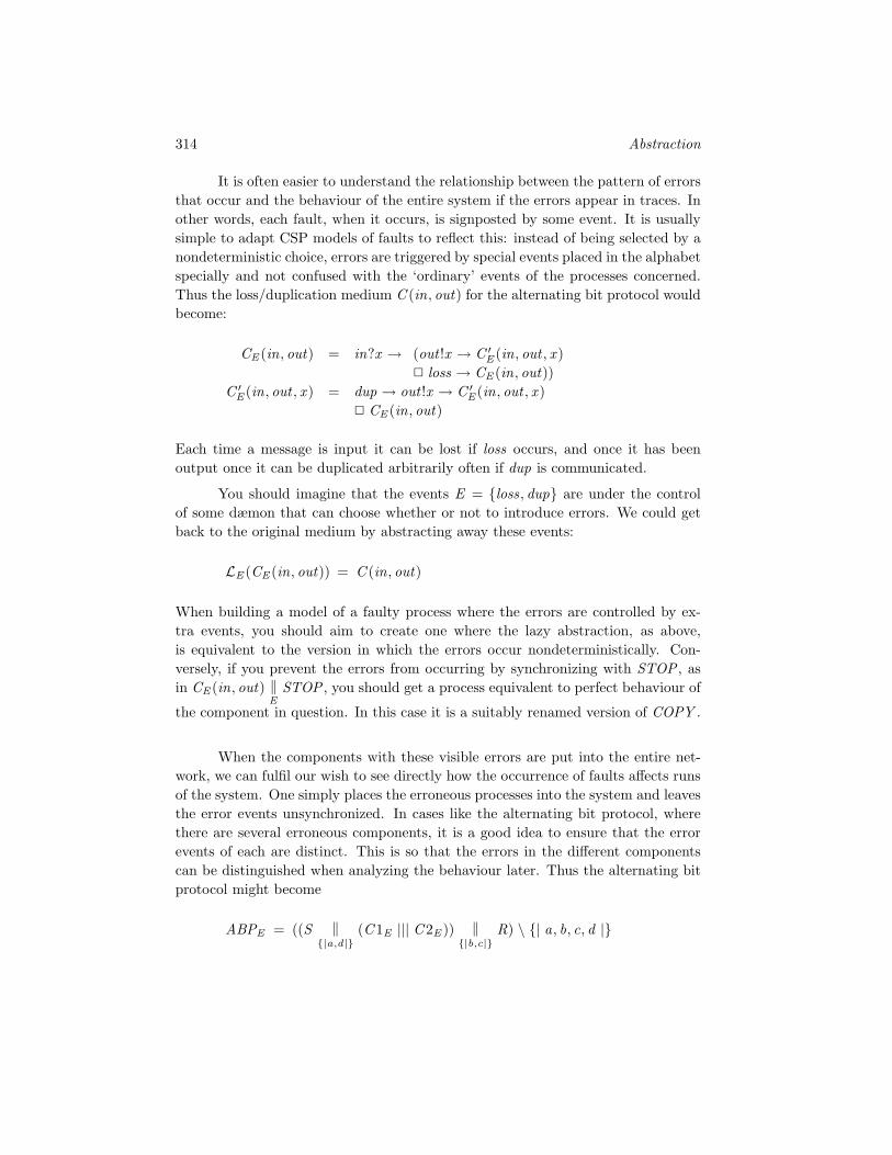
314 Abstraction
It is often easier to understand the relationship between the pattern of errorsthat occur and the behaviour of the entire system if the errors appear in traces. Inother words, each fault, when it occurs, is signposted by some event. It is usuallysimple to adapt CSP models of faults to reflect this: instead of being selected by anondeterministic choice, errors are triggered by special events placed in the alphabetspecially and not confused with the ‘ordinary’ events of the processes concerned.Thus the loss/duplication medium C (in, out) for the alternating bit protocol wouldbecome:
CE (in, out) = in?x → (out !x → C ′E (in, out , x )
loss → CE (in, out))C ′
E (in, out , x ) = dup → out !x → C ′E (in, out , x )
CE (in, out)
Each time a message is input it can be lost if loss occurs, and once it has beenoutput once it can be duplicated arbitrarily often if dup is communicated.
You should imagine that the events E = loss , dup are under the controlof some dæmon that can choose whether or not to introduce errors. We could getback to the original medium by abstracting away these events:
LE (CE (in, out)) = C (in, out)
When building a model of a faulty process where the errors are controlled by ex-tra events, you should aim to create one where the lazy abstraction, as above,is equivalent to the version in which the errors occur nondeterministically. Con-versely, if you prevent the errors from occurring by synchronizing with STOP , asin CE (in, out) ‖
ESTOP , you should get a process equivalent to perfect behaviour of
the component in question. In this case it is a suitably renamed version of COPY .
When the components with these visible errors are put into the entire net-work, we can fulfil our wish to see directly how the occurrence of faults affects runsof the system. One simply places the erroneous processes into the system and leavesthe error events unsynchronized. In cases like the alternating bit protocol, wherethere are several erroneous components, it is a good idea to ensure that the errorevents of each are distinct. This is so that the errors in the different componentscan be distinguished when analyzing the behaviour later. Thus the alternating bitprotocol might become
ABPE = ((S ‖|a,d|
(C1E ||| C2E )) ‖|b,c|
R) \ | a, b, c, d |

12.3 Abstracting errors: specifying fault tolerance 315
where S and R are as previously and
C1E = CE (a, b)C2E = CE (c, d)[[loss
′, dup′/loss, dup]]
We thus extend E to be loss , loss ′, dup, dup′.Having constructed a system with visible errors like this, we can either ab-
stract them immediately or put bounds on the circumstances in which they occurbefore doing so. It turns out that the first of these options is what is required forthe alternating bit protocol. The lazy abstraction LE (ABPE ) is the natural one tolook at: it is well-defined since ABPE is finitely nondeterministic and is, providedR and S are correctly defined as in Section 5.3, divergence-free. This form of ab-straction correctly reflects our expectations of this protocol, namely that an errorcan happen at any time but we should never rely on one happening. The fairnessassumptions built into lazy abstraction also correspond closely to the fact that theprotocol works provided the channels are not permitted to commit an infinite seriesof errors. If S and R are as defined in Section 5.3, it is true that
COPY LE (ABPE )
What this establishes precisely is that the alternating bit protocol refines this speci-fication provided only finitely many errors of any sort occur between each pair ofvisible actions. Another way of saying the same thing is that, whatever errors haveoccurred in the past, if whatever dæmon is selecting them stops doing so for longenough, the protocol will come into a state where it can make the progress requiredby the specification.
This lazy abstraction into non-error events gives what is probably the bestgeneral-purpose picture of the way a system with potential errors can behave underthe assumption that errors do not exclude everything else. However, what we haveshown in this case is not precisely the same as was proved in Section 10.3.1 where welooked directly at how infinite traces can analyze the protocol. There the infinitaryrelation was directly over the two internal channels, whereas here it is between theerrors and the external communications of the entire protocol. While the differencedoes not appear to be of great importance in this example, this is not always so:see Exercise 12.3.3. It teaches us one general lesson, namely that if you want torelate the errors that occur to some internal events of your system, then you mustdelay hiding the latter until after the comparison has been made.
The best way to assume a stronger bound on error behaviour than thatexpressed implicitly by lazy abstraction is by putting a constraining process inparallel with either the whole system or an appropriate part of it. Such a boundis likely to take one of two forms: either a limit on the total number of errors

316 Abstraction
that can occur through all time (perhaps with separate limits for different types oferrors) or a limit on how many errors can occur relative to some other behaviour, inwhich case, of course, the limitation must be imposed before any of the comparativeactions have been hidden.
Imagine, for example, a supposedly fault-tolerant processor built out of fouridentical units enclosed in a context which feeds them all identical inputs and gathersall their results.3 There are at least two different modes of failure of one of theprocessors: they might simply die in such a way that they never communicateagain (i.e., behave like STOP) or might become corrupted so that they can berelied on for nothing, not even not communicating (the most appropriate modelthen being ChaosA where A is the failing processor’s alphabet). In this latter casewe are assuming that a corrupted processor might, either through luck or, in someapplications, malice, do whatever it can to make the surrounding hardware’s jobas difficult as possible. A fault of this second sort is usually termed a Byzantinefailure.
If Proc is a process modelling the correct (and deterministic) behaviour of aprocessor without faults, then
(Proc halt STOP) byzantine ChaosA
gives a natural way of adding the potential for faulty behaviour. (P a Q is theinterrupt operator defined on page 239.)
Suppose that the result of composing the entire system, together with thesefaulty components and the harness used to manage the distribution and collectionof data to and from the four processors, is FTP (fault-tolerant processor).4 Theimportant thing from our point of view is that the four sets of fault events arepermitted to occur freely (i.e., they do not synchronize with each other or anythingelse). We will assume that the error events have become
E = halt .i , byzantine.i | i ∈ 0, 1, 2, 3
You would not expect FTP to work once all four processors have beenbrought down by faults. And Byzantine faults are likely to be harder to over-
3In any application like this it is vital that the programs running on the processors are de-terministic, since otherwise there might be several valid answers that the various copies couldproduce, almost certainly leading to confusion in the surrounding voting hardware!
4The mechanisms used to do this in the general case are really quite complex and would taketoo long to describe for this book. One of the major issues is the extent to which the harness itselfhas to be fault tolerant, since the advantages of running multiple copies of a processor are clearlyreduced significantly if you are dependent on some unreplicated piece of hardware to achieve ‘faulttolerance’. The mechanisms for achieving fault tolerance frequently use the timed dialect of CSPdescribed in Chapter 14. Some references can be found at the end of this chapter.

12.3 Abstracting errors: specifying fault tolerance 317
come than halting faults. It is, for example, reasonable to expect it to continueworking when all but one processor has halted, but it could not work when eventwo chaotic faults have appeared since the pair of faulty processors might agree ona different answer to a problem than the pair of correct ones; plainly there is no wayfor a voting system to distinguish which is right. If we wanted to prove that FTPwas tolerant of one Byzantine, or three halting, faults, the way to do this would beto prove that
LE (FTP ‖E
Halt(3)) and LE (FTP ‖E
Byzantine(1))
both meet an appropriate specification (see later), where, for example
Halt(n) = halt?i → Halt(n − 1)<I n > 0>I STOP
One of the major applications of the style of error modelling where the num-ber of faults is limited relative to some other set of events is in timed modelling,which we will meet in Chapter 14 and where you can express a bound on how manyerrors occur in a given interval. For example, you could state that no more than 3errors occur in any 13 time units. See page 416 for more on this.
In general, if you are imposing limits on how many errors occur, it will almostnever be appropriate to make an implicit assumption that errors definitely occur.This means that if the limit is expressed via the parallel composition
SystemE ‖A∪E
Limiter
where A is part of the alphabet of SystemE , then the process Limiter should neverrestrict which members of A occur. In other words,
LΣ A(Limiter) = RUN A
A process which satisfies this condition is said to be a monitor for A: its E behaviourcan depend on what it sees in A, but it will never refuse any communication in A.
If, for example, you want Limiter to express the condition that no more thanN errors occur for every M events in A, an appropriate process to use would be
Limit(E ,A,N ,M ) = Bound(E ,A,N ) ‖E
. . . ‖E
Bound(E ,A,N ) (M copies)
where
Bound(E ,A,n) = ?a : A→ Bound(E ,A,N ) ((?e : E → Bound(E ,A,n − 1))<I n > 0>I STOP)

318 Abstraction
is the process which prevents more than N error events happening for every Aevent. This subtle parallel composition expresses exactly the right condition ontraces via the way it synchronizes only on E : it acts as a monitor on A becauseeach Bound(N ) does. See Exercise 12.3.4.
The most extreme limitation on errors is to ban them outright. If E is the setof error events in a process SystemE modelled with visible errors (perhaps limitedin a less severe way), then
NoFaults = SystemE ‖E
STOP
represents its behaviour under the assumption that no error ever occurs. Thereis no need to abstract error events in this process since they never occur. Therefinement check
NoFaults LE (SystemE )
has a very interesting interpretation: it says that the system, with error eventspermitted to the extent allowed by the definition of SystemE , behaves no worsethan the error-free version. In other words, it asserts that SystemE is fault tolerantto the extent that it assumes faults can occur. The definition of lazy abstractionimplies that the reverse refinement relation holds for any process SystemE at all,so proving the above relation actually implies equivalence.
This gives a very clean definition of what it means for a process to be faulttolerant, and it is invaluable when faced with a system for which it is difficult togive a complete functional specification in a more abstract way. In using it youshould, however, realize that simply proving a system is fault tolerant does notmean it does what you intended. All it means is that any misbehaviour which ispresent in the version with faults is also there without. For example, the processChaosA∪E (which is, of course, refined by any divergence-free process with thisalphabet) is fault tolerant because it behaves no worse when faults are allowed thanwithout. Thus it is not, in general, the case that if P is fault tolerant and P Qthen Q is fault tolerant: fault tolerance is not a behavioural specification. (Unlikedeterminism it does satisfy a distributive law – see Exercise 12.3.5.)
Thus, if faced with the problem of developing a system which combines com-plex external behaviour with the need for fault tolerance, you should combine theabove refinement check with tests of whatever basic functional specifications (suchas freedom from deadlock and safety checks) seem appropriate. Of course, it wouldonly be necessary to prove these of the NoFaults version.
In conclusion to this section, it is the author’s opinion that the approachto modelling faults as controlled by visible actions, subsequently regulated and

12.3 Abstracting errors: specifying fault tolerance 319
error.0
error.1
error.2
Figure 12.1 Replicating data over multiple lanes (see Exercise 12.3.1).
abstracted, gives a more flexible and usually superior method than simply usingnondeterministic choices. The exceptions to its superiority are cases, such as over-coming a specified level of message corruption by replicating messages on page 121,where (i) there is no need to specify patterns of errors above a very low level, (ii) theoccurrence of errors is sufficiently bounded to avoid problems with divergence and(iii) the overall system behaviour is sufficiently simple so as to make the abstractspecification of fault tolerance above unnecessary.
By their nature, interesting complete examples of fault tolerance are moder-ately complex. Thus it was not possible to give as many examples in this sectionas we might have wished. The interested reader can, however, find various analy-ses based on the methods described in this section at the associated web site (seePreface for details).
Exercise 12.3.1 Define a buffer of bits (0, 1) which uses three error-prone channelsas shown in Figure 12.1. Channel i , after communicating the event error .i , may corrupt(but, for simplicity, does not lose) any bit it subsequently receives. Each bit is sentseparately through the channels and voted on at the other end.
Describe such a system and formulate a refinement check that asserts it is tolerantof one such error.
Exercise 12.3.2 Let P be any deterministic process with alphabet A. We can definea process
reboot(P) = P error reboot(P)

320 Abstraction
which reboots itself (back to initial state) each time the event error ( ∈ A) occurs. Definea context rebuild(·) which, though allowing all error events to occur, is such that
P = Lerror(rebuild(reboot(P)))
Hint: rebuild(Q) should record the external trace. Whenever an error event occursit should communicate that trace to Q so as to bring it back from its rebooted state to theone it was in before the error. Be careful to take account of any errors that occur duringthis rebuilding. It is helpful to use 1 → 2 renaming on the argument Q so that some of theevents it communicates are visible, but a second copy of them is available to be used whileresetting, and hidden. Specifically, you do not want to hide the ‘normal’ actions of Q, butneed to hide the rebuilding actions.
Why is it important that P is deterministic?
Exercise 12.3.3 Define a process Alt which alternately outputs 0 and 1 on channel c,and another Switch which inputs values on channel d and communicates the event switcheach time it inputs a consecutive pair of values that are different. Show that, as definedin this section, with CE as defined on page 314, the process
((Alt ‖|c|
CE (c, d)) ‖|d|
Switch) \ | c, d |
is fault tolerant.
Show that this behaviour is not preserved when CE (c, d) is replaced by the mediumprocess CN (c, d) defined on page 132 used in the original version of the alternating bitprotocol which guarantees to transmit at least one of each N messages and to duplicateeach no more than N times. How does the misbehaviour manifest itself?
This is an illustration of the effect mentioned in the text by which a system isconsidered fault tolerant, using the lazy abstraction definition, if it works provided thereare no more than finitely many faults between consecutive visible actions.
Exercise 12.3.4 Prove that the traces of Limit(E ,A, N ,M ) (page 317) are preciselythose members s of (A ∪ E )∗ satisfying
s = s 1 s 2 s3 ∧ #(s2 E ) > N ⇒ #(s2 A) ≥ M
Exercise 12.3.5 Suppose P and Q are both fault tolerant (in the sense defined usingNoFaults) with respect to the same set E of error events. Show that P Q is also faulttolerant.
12.4 Independence and security
In the first section of this chapter we imagined the existence of two users, and formedviews of how some process P looks to one of them with the other abstracted away.
12.4 Independence and security 321
Suppose they are working in a security conscious environment, and that Hugh hasa higher security classification than Lois. It is a problem of considerable practicalimportance to understand when information about what Hugh is doing can get toLois via their joint use of P . You can imagine the following scenarios:
(a) Lois, a spy, attempts to find out about Hugh’s interactions with P , theassumption here being that Hugh is unaware of Lois’s presence.
(b) Hugh is a ‘mole’, namely an agent working in the high security levels of hisenemies. He is trying to set up a ‘covert channel’ with Lois, who is his friendon the outside, so that the information he has learned can be relayed back totheir spy-masters. Therefore they try to use P to get information from oneto the other, and may well have agreed some code in advance.
Though the second of these is, on the face of it, the more challenging problemfor the process designer from the point of view of counter-espionage, in an absolutesense they are the same. If no information about what Hugh does ever leaks throughto Lois (i.e., P is secure in the sense (a)) then automatically no covert channelcan exist since anything a malicious Hugh does under (b) to pass information, aninnocent one under (a) might have done ‘by accident’. It is only when consideringimperfect systems that the two modes should perhaps be differentiated.
Clearly what is important is Lois’s abstracted view of P . She can only seewhat Hugh is doing if what he does affects what she sees. What we are trying tospecify is what one can either view non-interference (i.e., what Hugh does does notinterfere with what Lois sees) or independence (i.e., what Lois sees is independentof Hugh). The latter of these two terms is more appropriate for the applications wenow have in mind. A very clear specification of this is simply that Lois’s view isdeterministic: you can think of Hugh as a nondeterminism resolving dæmon withinan abstraction such as LH (P), so if the abstraction is actually deterministic thennone of his choices is reflected in what she sees. You should use either lazy or mixedabstraction depending on the nature of the interface between Hugh and P .
For a finitely nondeterministic, divergence and -free process P we can thusdefine
• P is lazily independent from H (written LINDH (P)) if and only if LH (P) isdeterministic, and
• P is mixed, or transaction5 independent from H , with respect to the set ofsignals S (written MIND
SH (P)) if and only if MS
H (P) is deterministic.
5The term transaction independence (used by Wulf [138]) derives from the most common useof mixed abstraction: interpreting the output phases of transactions such as those seen in thememory example on page 307 correctly.

322 Abstraction
There is a clear connection between this definition and Corollary 12.1.3, sinceit is evident that the condition of separability is closely related to security. Afterall, a process which is built as the parallel composition of two processes which donot synchronize and respectively serve only Hugh and only Lois is self-evidentlysecure. Indeed, some authors have used it as one definition of non-interference/independence. It has two disadvantages: the easier to understand is that it isclearly symmetric whereas independence is not. We do not mind Hugh being ableto see what Lois can do, since we have not banned information flowing that way.We will discuss the second disadvantage later.
The best way to understand our definitions is to see some examples. LetL = l , l1, l2, ls1, ls2, H = h, h1, h2, hs1, hs2 and S = ls1, ls2, hs1, hs2 (theset of signal events). The following simple processes show the main ways securityand insecurity manifest themselves.
1. Let P1 = h → l → P1. This is insecure because LH (P1) = Chaosl, whichis nondeterministic. Intuitively, this process is insecure because Lois can seeexactly how many events Hugh has performed.
2. On the other hand, P2 = (h → l → P2) (l → P2) is secure, sinceLH (P2) = µ p.l → p. It is not, however, separable since the abstraction intoH is nondeterministic. The fact that l can always occur means that Lois canno longer count h’s by counting l ’s.
3. Define
P3 = l1→ P3′
h1→ P3
P3′ = l2→ P3 h2→ P3′
P3 is secure since LH (P3) = µ p.l1→ l2→ p. It is not secure in the reversedirection since
LL(P3) = µ q .(h1→ q) (h2→ q)
The point is that only Lois controls which state (P3 or P3′) it is in, butHugh can detect the state by looking which of h1 and h2 is permitted. Thusinformation can pass from Lois to Hugh but not back.

12.4 Independence and security 323
4. The following process, unlike those seen so far, uses signal events:
P4 = l1→ ls1→ P4 l2→ ls2→ P4 h1→ hs1→ P4 h2→ hs2→ P4
You can think of this process as one that both Hugh and Lois can ask ques-tions of by inputting values, and it gives them the appropriate answer backas a signal. The lazy abstraction of this process is nondeterministic, since ifHugh could delay the events hs1 and hs2 then Lois could tell he was doingso (and had input some value). The mixed abstractionMS
H (P4) is, however,deterministic and so this process satisfies MIND
SL(·). This is appropriate,
since its behaviour towards Lois does not depend on what Hugh has done.
5. If Hugh is certain to receive a signal at some point then the fact that he doesdoes not convey information to Lois. Thus the following process satisfiesMIND
SL(·), since to Lois it looks exactly like µ p.l → p.
P5 = hs1→ l → P5
6. On the other hand, if Lois can tell something about which signal Hugh re-ceived, then we get an insecure process, and indeed
P6 = hs1→ l1→ P6 hs2→ l2→ P6
fails the mixed condition. This only applies when, as in this example, thevalue Hugh gets is not predictable on the basis of what Lois legitimatelyknows.
Now look back to the memory example on page 307. The work we did thereshows that this is secure, for | T |> 1, if and only if there is no location that Hughcan write to and Lois can read. This is, of course, exactly what one might expect.This is perhaps the simplest of a wide range of situations where our two users areboth reading and writing to some system. Some extensions that can lead to furthersecurity difficulties are listed below.
• They might be reading and writing to files, which have to be created usingsome name. It is possible for information to flow by Lois testing, by tryingto create a file with a given name, whether Hugh has one of the same nameopen. (This assumes that either user will have a request to create a filerefused if the other has one with the chosen name.)

324 Abstraction
• There might be contention for resources: if what Hugh does affects whetherthere is room (in memory, on disk etc.) for an action of Lois to be executed,then information can flow.
• Instead of the transactions on the data being only atomic reads and writes,they may comprise series of actions which require locks to be placed on somedata items (usually non-exclusive read locks or exclusive write locks). IfHugh were to place a read lock on a location Lois wants to write to, then itis possible for information to flow.
All of these situations have been dealt with successfully via the methods describedin this chapter. For more details, see [123, 138] and the worked examples on theweb site (see Preface).
Example 12.4.1 (sharing a communication medium) Interference, and henceinformation flow, can also appear in other applications where high-level and low-level processes share resources. One of these is shared communication media. Sup-pose Hugh and Lois respectively want to send messages to Henry and Leah, whoshare their security clearances. Consider the network
Comm1 = ((SendH ||| SendL) ‖|in|
Medium) ‖|out|
(RecH ||| RecL)
where
SendL = send .lois?x → in.lois.leah!x → SendL
SendH = send .hugh?x → in.hugh.henry !x → SendH
RecL = out .leah?x → rec.leah!x → RecL
RecH = out .henry?x → rec.henry !x → RecH
Medium = in?s?t?x → out !t !x → Medium
Even though the high-level processes cannot send messages to the low-levelones through this system, it does not satisfy the obvious lazy security property.Despite the buffering provided at the two ends, it is possible for the high-levelprocesses to block up the network if Henry refuses to accept the messages thatarrive for him. This means that the low-level lazy abstraction is nondeterministic:the low-level processes can detect certain high-level activity via their own messagesbeing blocked.
The following two solutions illustrate much more widely applicable methodsfor overcoming security problems which arise, like this one, from contention forresources.
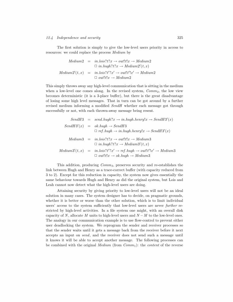
12.4 Independence and security 325
The first solution is simply to give the low-level users priority in access toresources: we could replace the process Medium by
Medium2 = in.lois?t?x → out !t !x → Medium2 in.hugh?t?x → Medium2′(t , x )
Medium2′(t , x ) = in.lois?t ′?x ′ → out !t ′!x ′ → Medium2 out !t !x → Medium2
This simply throws away any high-level communication that is sitting in the mediumwhen a low-level one comes along. In the revised system, Comm2, the low viewbecomes deterministic (it is a 3-place buffer), but there is the great disadvantageof losing some high level messages. That in turn can be got around by a furtherrevised medium informing a modified SendH whether each message got throughsuccessfully or not, with each thrown-away message being resent.
SendH 3 = send .hugh?x → in.hugh.henry !x → SendH 3′(x )
SendH 3′(x ) = ok .hugh → SendH 3 ref .hugh → in.hugh .henry !x → SendH 3′(x )
Medium3 = in.lois?t?x → out !t !x → Medium3 in.hugh?t?x → Medium3′(t , x )
Medium3′(t , x ) = in.lois?t ′?x ′ → ref .hugh → out !t ′!x ′ → Medium3 out !t !x → ok .hugh → Medium3
This addition, producing Comm3, preserves security and re-establishes thelink between Hugh and Henry as a trace-correct buffer (with capacity reduced from3 to 2). Except for this reduction in capacity, the system now gives essentially thesame behaviour towards Hugh and Henry as did the original system, but Lois andLeah cannot now detect what the high-level users are doing.
Attaining security by giving priority to low-level users will not be an idealsolution in many cases. The system designer has to decide, on pragmatic grounds,whether it is better or worse than the other solution, which is to limit individualusers’ access to the system sufficiently that low-level users are never further re-stricted by high-level activities. In a file system one might, with an overall diskcapacity of N , allocate M units to high-level users and N −M to the low-level ones.The analogy in our communication example is to use flow-control to prevent eitheruser deadlocking the system. We reprogram the sender and receiver processes sothat the sender waits until it gets a message back from the receiver before it nextaccepts an input on send , and the receiver does not send such a message untilit knows it will be able to accept another message. The following processes canbe combined with the original Medium (from Comm1): the content of the reverse

326 Abstraction
messages is irrelevant.
SendL4 = send .lois?x → in.lois .leah!x → out .lois?x → SendL4
SendH 4 = send .hugh?x → in.hugh.henry !x → out .hugh?x → SendH 4
RecL4 = out .leah?x → rec.leah!x → in.leah.lois .Zero → RecL4
RecH 4 = out .henry?x → rec.henry !x → in.henry .hugh.Zero → RecH 4
The resulting Comm4 is not only secure, it is separable and equivalent to thecomposition of a one-place buffer (i.e., COPY ) between each of the two pairs ofprocesses. Note that the medium is used more than previously, since two internalmessages are required for each external one, but it is used more carefully as eachtime one of the four processes around it sends a communication to it on in, it isimpossible for the resulting out to be refused. (End of example)
We have seen that the natural specifications of both security and fault toler-ance involve similar ideas. They are, in fact, closely related specifications. SupposeLINDH (P) holds. The determinism of LH (P) easily implies that it equals
LH (P ‖H
Q)
for any divergence-free process Q with alphabet H . This is reassuring, since itmeans that what Lois sees does not depend on what high-level process we put inparallel with P . It also means that
LH (P) = P ‖H
STOP
and so P is ‘fault tolerant’ if you think of the high-level actions as the errors. Thisis not surprising, since if there is no way of telling, by looking at the pattern of aprocess’s behaviour in its non-error alphabet, what, if any, errors have occurred,then it must be fault tolerant!
On the other hand, a process can be fault tolerant without the abstraction
LE (P)
being deterministic, so the reverse implication does not hold. The difference is that,when considering fault tolerance we have an inbuilt standard to judge the processagainst, namely the way it behaves without errors. If it should happen that someerror resolves a nondeterministic choice which would have had to be made anyway,this does not matter in judging fault tolerance, but it might convey information tothe user about the pattern of errors. See Exercise 12.4.2 for a class of examples.
12.4 Independence and security 327
In real applications one will frequently have more than just the two securitylevels we have modelled in this section. One could have any number with a partialorder security policy relating them: user Ui ’s behaviour can affect Uj if and only ifclearance(i) ≤ clearance(j ). There is, however, no need to extend our theory furthersince all you have to do is to show that, for each security level λ, the collection ofall users with this level or below is independent of the collection of all the others.Thus you simply look at a series of two-way partitions of the overall alphabet. Forexample, if there is another user Mhairi with alphabet M whose clearance is mid-way between Hugh’s and Lois’s, then to establish security of a process P you shouldprove
LINDH∪M (P) and LINDH (P)
i.e., neither Hugh nor Mhairi can influence what Lois sees, and Hugh cannot influ-ence what Lois and Mhairi see.
The limitations of security modelling
Security modelling is a subject full of philosophical difficulties, and just about allspecifications of what it means for a process to be ‘secure’ can be criticized in oneway or another. A general text is not the place to go into this in detail, but it is aswell to understand just what our particular specification can and cannot do.
First and foremost, a security specification couched in a particular model canonly reflect information flow via the sort of behaviour the model records. The mostobvious thing missing from the models we have used is timing information, and itis certainly possible to construct examples which appear secure over N which onewould suspect might contain ‘timing channels’ if implemented in the obvious way.The various secure communication examples above, such as Comm4, come into thiscategory as the low users will presumably get a variable bandwidth depending onthe level of activity of Hugh and Henry.
By and large, the more detailed a model one chooses, the more complexboth process modelling and security analysis become, and (presumably) the morelikely we are to find small flaws in security. All one can do is to pick one’s modelintelligently and be aware of the limitations built into the choice.
As we will see in Chapter 14, it is possible to take time into account in mod-elling CSP. There is no reason in principle why the determinism-based specificationcould not be used to specify security over that sort of model too.
There is a clear sense in which the determinism-based condition can be viewedas too strong. It only defines as secure those processes whose low view-point is de-terministic. However, it is undoubtedly possible to build a secure process whose
328 Abstraction
low-level abstraction is nondeterministic, since the mechanism resolving the non-determinism has nothing to do with how the high interface behaves. For example,there are many separable processes whose low-level abstraction is nondeterministic,and clearly any process implemented as an interleaving of entirely disjoint high andlow-level processes is secure. In this sense,
ChaosH∪L = ChaosH ||| ChaosL
is secure.The point you should try to understand, however, is that just because one
implementation of a given process is secure, this is no guarantee that all are. Forexample, if LEAK is any divergence-free process whatsoever, for example
µ p.hugh?x → lois !x → p
you would not naturally think of
ChaosH∪L LEAK
as secure since it is free to behave like LEAK every single time it is used. Theabove process is, however, equivalent to ChaosH∪L, and we thus have two processdefinitions that none of our semantic models can tell apart, one being plainly secureand one insecure. Perhaps the problem is that our models go to great lengths torepresent nondeterminism as abstractly as possible, and specifically do not give usinformation about whether a given nondeterministic decision is resolved innocentlyor in a way that allows information to flow.
A number of authors have attempted to define conditions to decide whethera general CSP process is secure in the sense we have being trying to capture. In-variably these conditions are satisfied by ChaosH∪L, even though this process isrefined by many others which do not satisfy them. We might call this the refine-ment paradox. The idea that P can be secure and Q P insecure is contrary toall our understanding of what refinement means. Reassuringly, it is true that ifLINDH (P) and P Q then LINDH (Q), because by construction
P Q ⇒ LH (P) LH (Q)
and the only refinement of a deterministic process is itself. In truth, it simply is notpossible to determine whether a general process is secure by looking at its value inthe standard denotational models of CSP.
A good analogy is provided by deadlock freedom: if P is deterministic youcan tell if it can deadlock by looking at its value in T , but for general processes youneed a richer model like N . Similarly, if P is low-deterministic6 in the sense that
6Any deterministic process is low-deterministic, as is any process satisfying LINDH (·).

12.4 Independence and security 329
for all traces s and a ∈ L
s 〈a〉 ∈ traces⊥(P) ⇒ (s , a) ∈ failures⊥(P)
then you can accurately decide whether or not it is secure from its value in N . Forvalues outside this class, like ChaosH∪L, they do not give enough information.
Just how much finer a model is required to deal with the general case isdebatable: certainly you need something about as fine as that provided by theoperational semantics in Chapter 7, and arguably you should incorporate probabilityas well. In any case it is very unlikely that such an attractive, persuasive, orpractical (thanks to FDR’s ability to check determinism: see page 225) definitioncan be found.
Exercise 12.4.1 Recall from page 317 that a monitor for a set A of events is one thatnever refuses any member of A. Say that P is semi-separable with respect to (H ,L) if thereis a monitor M for L and a process PL using only events from L such that P = M ‖
LPL.
(a) Show that if P is separable then it is semi-separable.
(b) Suppose P is semi-separable (into (M ,PL) as above) with respect to (H ,L). Showthat LH (P) = PL for such P . Deduce that if PL is deterministic then LINDH (P)holds.
(c) Now suppose that P is such that LINDH (P). Let M be the process whose failuresare
(s,X ∩ H ) | (s,X ) ∈ failures(P)∪ (s 〈l 〉 t , Y ) | Y ∩ L = ∧ s ∈ traces(P) ∧ 〈l 〉 t ∈ L∗ ∧ l ∈ initials(P/s)
Show that M is a monitor such that P = M ‖L
LH (P) and hence that P is semi-
separable.
Exercise 12.4.2 Let P be any divergence-free process with alphabet H ∪ L. Showthat P ′ = P ChaosL satisfies the definition of fault tolerance
P ′ ‖H
STOP LH (P ′)
but need not be secure.7
7There are a number of definitions of ‘security’ in the literature which would define such P ′ tobe secure for all P , even though if with P = LEAK from page 328, for example, you can guaranteethat if Hugh communicates anything with P ′, then Lois gets to hear it.

330 Abstraction
12.5 Tools
With the exception of the fine distinctions made at the start by the interpretationof abstraction over infinite traces, just about everything in this chapter is relevantto FDR. The ways of structuring the checking of specifications using abstractionboth helps in formulating the properties you want of processes and in using thetool’s compression functions (see Section C.2).
We have seen various applications of determinism checking in this chapter,in the sense that it has been used to characterize security and separability. FDR’sability to check determinism was included mainly because of these results. Notethat because of the way lazy and mixed abstraction are formulated it will often benecessary to use the stable failures model F for these determinism checks, just as itis used for refinement checks involving abstraction. For the only formulation of lazyabstraction which can be rendered in finitely nondeterministic CSP is the one onpage 303 which, if interpreted over N , often introduces false divergences that wouldconfuse FDR. This means that you are, in fact, checking a process that might welldiverge for F-determinism as discussed on page 221. This is only a technicality,however, since the F-determinism of LF
H (P) is equivalent to the (true) determinismof the other two formulations of LH (P).
All the significant examples from this chapter, and several larger applicationsof the definitions of fault tolerance and security, can be found on the web site.
12.6 Notes
The work in this chapter has developed over the past three years, with many of theresults arising from Lars Wulf’s doctoral studies with the author: his thesis providesby far the most extensive study of the compositional properties of abstraction andits application to security. Jim Woodcock was very influential on the early phasesof this work.
The precise formulations of lazy and mixed abstractions in this chapter arenew. They are direct descendants of the versions used in [109, 123, 124] which werebased on a definition of lazy abstraction using interleaving:
L|||H (P) = P ||| RUN H
The intuitive justification for that form of abstraction is that the process RUN H
camouflages events in H : you can never get any information about P from such anevent occurring since it could always have come from RUN H .
The one advantage of the earlier version is that it is easily definable usingstandard operators over N , while we have had to compute ours over F (in the

12.6 Notes 331
knowledge that the N version is, in fact, the same). It has at least three disadvan-tages. The first is that it is not natural to have an abstraction into L performinglots of events in H , with the consequence that many of the results and definitionswe have formulated do not work as neatly since they have to take account of thecamouflage events. The second is that the corresponding way of lifting a specifi-cation on L to one on the whole alphabet (implied by the second part of Exercise12.2.2) does not lend itself nearly as well to facilitating compression.
The third and main disadvantage is that L|||H (P) is not quite abstract enough:
it identifies strictly less processes than LH (P). If the event l ∈ L is only possibleafter h ∈ H this is still true of the interleaving abstraction. Thus if
P1 = STOP l → STOP
P2 = h → l → STOP
P3 = h → h → l → STOP
we have that LH (Pi) are all the same, but L|||H (Pi) are all different. The interleaving-
based abstraction of P1 has the trace 〈l〉, whereas the shortest traces of the otherabstractions containing an l are respectively 〈h, l〉 and 〈h, h, l〉. Intuitively, theinterleaving definition gets this wrong since surely all these three processes actuallydo look the same in L.
Having seen this example you might wonder why the interleaving definitionwas ever used, but in fact this difference does not show up in three of the mostimportant applications of lazy abstraction. Thanks to the result contained in thesecond part of Exercise 12.2.2, noting that
NoFaults = P ‖E
STOP
never communicates in E , we get that P is fault tolerant in the sense describedearlier if and only if
L|||E (NoFaults) L|||
E (P)
So it yields an identical definition of fault tolerance.
It can be shown that LH (P) is deterministic if and only if L|||H (P) is. This
is left as an (interesting) exercise. It follows that independence defined in terms ofthe determinism of either abstraction is identical, and that a deterministic processis separable if and only if both L|||
H (P) and L|||L (P) are deterministic.
An example of the use of abstraction in formulating fault tolerance propertiescan be found in [141]. Earlier fault tolerance case studies such as [14] have usedspecifications crafted to the examples under consideration.

332 Abstraction
There have been numerous definitions of security, in the sense of indepen-dence/non-interference, over CSP models. Several of these, namely those of [125, 2,44, 38] turn out to be equivalent to ours for deterministic P , though they usuallymake the decision to extend their definitions over all processes rather than restrict-ing them to the low-deterministic processes or a subset. That usually leads to theirconditions passing processes that appear decidedly suspect.
An exception to this problem is the work of Forster [38], who develops con-ditions on labelled transition systems that are both equivalent to ours for low-deterministic processes and which are extremely careful not to admit any insecureprocesses – at least provided one interprets labelled transition systems in a partic-ular way. That is, he insists that when a process’s operational semantics produce agiven labelled transition system, all the potential behaviours displayed in the LTSmust actually be possible in every implementation. In other words, there must beno implementation decisions taken that refine away some options. In this possiblis-tic view of processes, where the range of potential behaviours may not be reduced,the concept of refinement more-or-less has to be discarded. While this is hardlywelcome, the fact that we lose the refinement paradox with it is some compensa-tion.
His conditions themselves are very simple in concept. They essentially statethat the result of each high-level action in any state σ is equivalent, in the lowview produced by banning all subsequent high actions, to the same low view of σ.Though generalisations of lazy independence, they are nevertheless still very strongconditions, perhaps chiefly because they look at LTS’s as basically sequential thingswhere all actions subsequent to a given one are influenced by it. Perhaps for thatreason they seem to be good at handling examples in which nondeterminism is usedto mask8 potential insecurities arising in the low-level user’s interactions with thesame process in a network, but not at handling ones in which the nondeterminismis introduced by a different one.
Forster named his conditions (there are variations based on different processequivalences and different ways of handling the case where a given state has severalcopies of the same high-level action) local non-interference. An implementation ofperhaps the main variant has since been included in some versions of FDR.
Both Forster’s thesis [38] in which the conditions are described in detail, andseveral example files, can be found via the web site of this book.
Though we have, of course, couched our determinism-based definition of se-curity in the models of CSP, one can argue that it is largely independent of which
8This typically means that an analysis is done to discover what range of behaviours might bevisible to low as a result of different high-level choices, and we ensure that these choices are alwayspresent whatever high has done.

12.6 Notes 333
process algebra equivalence is used. This is explained in [109] and illustrated in[37].
2005: The work on noninterference in this chapter has recently been extendedto timed processes of the form found in Chapter 14.


Part III
Practice


Chapter 13
Deadlock!
We have already met several examples of deadlock, which is certainly the best-known pathology of concurrent systems. It is also – probably for this reason – themost feared. A system becomes deadlocked when no further progress can be made.We distinguish it from livelock, where an infinite amount of internal progress isbeing made without any interaction with the external environment, even thoughfrom the outside a deadlocked and a livelocked system look similar. Internally thetwo phenomena are quite unalike, meaning, for example, that different techniquesare needed for analyzing when they can appear.
In the first section we find out how deadlock arises, how to eliminate dead-locks arising for local reasons, and hence how to eliminate deadlock in tree networks.There are various useful ad hoc conditions on networks, many based on orderings,which can be used to eliminate deadlock; these are surveyed in the second sec-tion. The third section looks at some more general global techniques for deadlockavoidance. The fourth shows how the construction and topology of a network cansometimes allow us to factor its deadlock analysis into a number of smaller parts.The fifth section looks at the limitations of the style of local analysis we advocate.
13.1 Basic principles and tree networks
13.1.1 Assumptions about networks
We cannot detect or reason about deadlock using traces alone. After all, for anyprocess P ,
traces(P) = traces(P STOP)

338 Deadlock!
and the right-hand side can deadlock immediately whether or not the left-hand sidecan. Deadlock is best described in the stable failures model of CSP, where it isrepresented by the failure (s , Σ ∪ ) for s any trace in Σ∗. (The fact that aprocess does nothing after it terminates should not be regarded as deadlock.) Infact, systems in which both deadlock and termination are simultaneously an issueare (at least in the author’s experience) very rare and it would be an unnecessarycomplication to have to deal at every turn with the case of processes or networksterminating. This leads us to make the first of a number of assumptions aboutthe sorts of network we are dealing with. These are all things we will assumethroughout the first four sections of this chapter, since they all help in pinningdown and reasoning about deadlock in realistic systems.
(A) Throughout this chapter we will assume that none of the component pro-cesses of our networks can terminate (though this does not preclude thembeing constructed out of sub-processes that can).
Deadlock is a static condition: when it happens no process is making progressand, in particular, both the shape of the network and the states of all the processesin it are, from that moment, fixed. This leads to our second assumption about thenetworks we are considering:
(B) We will consider only statically-defined networks ‖n
i=1(Pi ,Ai), where the
communications of Pi are entirely within Ai .
This does not mean we are excluding dynamically-growing networks such as thosewe can build with piping and enslavement, merely that one would have to take asnapshot of such a network at the moment of deadlock and think of it in our newterms. The use of the alphabetized parallel operator means we have excluded usesof ||| and ‖
Xwhere there are some events that can be communicated independently
(i.e., without synchronization) by more than one process. We want to know exactlywhich process or processes participate in each event. The majority of practicaluses of ‖
Xand ||| could be written in this way since they do not use the power
of those operators to introduce ambiguity about which process performs an event.In practice we will allow the use of these operators as long as the network couldhave been built using the alphabetized parallel operator. What we have done isto concentrate on ‘realistic’ style compositions, at the expense of forms of parallelcomposition which are mainly used for establishing specification effects. This isequally true of our next assumption:
(C) We will consider only networks that are triple-disjoint, meaning that thereis no event that requires the synchronization of more than two processes. In

13.1 Basic principles and tree networks 339
other words, if Pi , Pj and Pk are three distinct nodes in the network, thenAi ∩Aj ∩ Ak = .
Thus all events are either communications between a pair of processes, or are simpleinteractions between a single process and the environment. All interaction withinthe network must be point-to-point. The main thing that this excludes is the useof parallel composition as the many-way conjunction of trace specifications.1
Implicit in assumption (B), but sufficiently important that it should be stateddirectly, is the following:
(D) We consider only networks built using parallel composition from their com-ponent processes. In particular, they contain no renaming or hiding.
Since the majority of networks one meets in practice violate this, especially becauseof the hiding of internal communications, this looks like an over-strong assumption.The reason why we make it is to allow us to concentrate on a single central case andto see the communications of all the component processes of a network directly. Twobasic facts and a series of laws mean that we can always transform any reasonablenetwork into one which is, from the point of view of deadlock, equivalent and whichmeets condition (D). The two facts are:
• P is deadlock-free if, and only if, P \ X is for any X ⊆ Σ. (P \ X may beable to diverge when P cannot, but see Section 8.4.)
• P is deadlock-free if, and only if, P [[R]] is for any alphabet transformation Rwhich contains all of P ’s events in its domain.
Intuitively these are both obvious: since deadlock means reaching a state where noaction of whatever name and whether visible or invisible is possible, it does notmatter if the actions are renamed or hidden.
The laws referred to are just 〈hide-X ‖Y -dist〉 (3.7), 〈f [·]-X ‖Y -dist〉 (3.10),〈f [·]-hide-sym〉 (3.11), and 〈f [·]-hide-null〉 (3.12).
These usually allow us to move all the hiding to the outside of a parallelcomposition, and all the renaming onto the individual component processes. Thehiding is then irrelevant from the point of view of deadlock, and the renaming sim-ply creates new (and necessarily busy if the originals were) component processes.(Two of these laws are restricted to 1–1 renaming, but fortunately it is that sort ofrenaming which is generally used in the construction of realistic models of imple-mentations – typically modularized into operators like >> and //.) An example isgiven at the end of this chapter in Section 13.7.
1In that case, deadlock is likely to arise because of ‘inconsistency’ in the specifications: theyallow a trace s but no continuation of s.

340 Deadlock!
Our final assumption is much easier to understand than the one above:
(E) We assume the network is busy, defined to mean that each component processis deadlock-free.
While there are many deadlock-free networks that do not satisfy this, the deadlocksoccurring in their individual processes usually fall into one of the following twocategories:
• states (often error states) which in fact – and often because of the correctfunctioning of the network – the component process never reaches; and
• the component process that is deadlocking is one (most often the processSTOP itself) which is an ‘extra’ process designed to prevent some undesirableevent from happening in the main network.
In the second case one can usually (and always when the offending process is STOP)just redesign the individual processes so that they simply avoid the offending be-haviour rather than require an externally imposed ban. To expect a deadlock analy-sis technique to be able to handle the first case is like using a screwdriver to hammerin a nail – one should not expect it to be able to analyze trace conditions of in-dividual component processes. Thus this assumption of busy-ness is a reasonablestarting point for examining deadlock behaviour per se.
Finally we make an assumption about the way we describe processes ratherthan about the processes themselves. The concept of a channel in CSP is ratherbroad, and in general many processes may share events from the same channel (i.e.,the events c.x for the name c) even when the network is triple-disjoint. This istypically because the name c really represents an array of ‘real’ channels. Through-out our discussions of deadlock, the word channel will be restricted to this ‘real’sense: a collection of events used either by a single process to communicate withthe environment, or by a pair of processes to talk to each other. In other words,any channel that intersects the alphabet of a process is contained in it. There isalso the implication in the word ‘channel’ that communications over it are somehowwell-behaved and co-ordinated. This is an idea we will be able to make clearer atthe end of the next section.
This completes our base assumptions. Though they may seem severe, theintention is only to concentrate on the central cases of deadlock and to give ourselvesa common language to talk about the systems we are considering. In fact we willfind that the methods used to combat deadlock are often phrased in a way that isnot specific to our tightly-defined class of networks, merely to the class of networksthat could be transformed into it in the ways described above.

13.1 Basic principles and tree networks 341
13.1.2 Ungranted requests and conflicts
The assumption of triple-disjointness gives particular importance to the concept ofa communication graph, something we first discussed in Section 2.2, for this graph(a node for each process and an edge between a pair if their alphabets intersect)now ‘shows’ all the interactions between processes. The essence of any deadlockstate will be the collection of requests for communication that processes are makingto each other along the edges of this graph.
We might as well assume that this graph is connected (i.e., that there is a paththrough the edges between any chosen pair of nodes). If it were not connected thevarious connected components into which it divides can be thought of as completelyindependent processes from the point of view of deadlock analysis.
Since deadlock is a static phenomenon, we can examine the fixed state inwhich it occurs. Each component process is in a state which we can add to thecommunication graph. Because of our assumption of busy-ness, each process mustbe able to perform some action. In general this might be either one which doesnot require the agreement of any other process or (because of triple-disjointness)one which requires the agreement of exactly one other process. The first of these(which breaks into two cases: internal (τ ) actions and ‘external’ communications)cannot be the case in a deadlock state since there would be nothing in the networkpreventing the action – meaning that it was not deadlocked. Therefore every processmust have one or more requests to other processes – necessarily ones that do notagree to any of the requested actions.
Thus, all of the interest in a deadlock state is concentrated on the set ofcommunications that are shared by two processes: we will call this set
⋃Ai ∩ Aj | i = j
the vocabulary of the network.
Suppose P and Q , with alphabets A and B , are processes in the networkwhich can communicate with each other (i.e., A∩B = ). We define an ungrantedrequest to exist from P to Q in the state σ (the details of which we will discuss later),written P σ=⇒•Q , if neither process can communicate outside the vocabulary of thenetwork; P can communicate in B but they cannot agree on any communication inA ∩ B .
Ungranted requests are the building blocks of a deadlock. We can form asnapshot graph of a deadlock by superimposing the (directed) arcs representing themonto the communication graph. A possible example is shown in Figure 13.1 (wherethe dotted lines represent edges of the communication graph with no ungrantedrequest). We should notice that any ungranted request which appears between a

342 Deadlock!
e
a
b
d
c
Figure 13.1 Typical snapshot graph of a deadlock state.
pair (Pi ,Pj ) of processes in the entire network can also appear when Pi and Pj areput in parallel (only) with each other.
There are very good reasons why as much as possible of the analysis (whetherfor deadlock or anything else) of a large network should be done locally rather thanconsidering the whole system all the time. The patterns of behaviour that occurbetween small and localized collections of processes are much easier to understandboth for humans and computer tools – the latter because of the state-space explosionwhich occurs as networks grow. The various assumptions (A)–(E) above are allconditions that apply to an individual process (i.e., are local in the strongest sense),and it is clear that enumerating the ungranted requests between pairs of processesis also very local.
Start from any process P0 in a deadlocked network. It has an ungrantedrequest to another process P1, which in turn has an ungranted request to some P2,and so on. Since the network we are looking at is finite this sequence must repeat,giving a cycle of processes
〈Pr ,Pr+1, . . . ,Pr+s−1〉
where Pr = Pr+s . This simple argument, and the chains and cycles of processes itcreates, are central in deadlock analysis.
Look again at Figure 13.1. Wherever you start here, and whatever choices
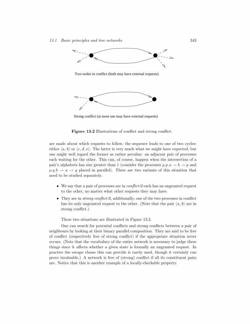
13.1 Basic principles and tree networks 343
Two nodes in conflict (both may have external requests)
Strong conflict (at most one may have external requests)
Figure 13.2 Illustrations of conflict and strong conflict.
are made about which requests to follow, the sequence leads to one of two cycles:either 〈a, b〉 or 〈c, d , e〉. The latter is very much what we might have expected, butone might well regard the former as rather peculiar: an adjacent pair of processeseach waiting for the other. This can, of course, happen when the intersection of apair’s alphabets has size greater than 1 (consider the processes µ p.a → b → p andµ q .b → a → q placed in parallel). There are two variants of this situation thatneed to be studied separately.
• We say that a pair of processes are in conflict if each has an ungranted requestto the other, no matter what other requests they may have.
• They are in strong conflict if, additionally, one of the two processes in conflicthas its only ungranted request to the other. (Note that the pair 〈a, b〉 are instrong conflict.)
These two situations are illustrated in Figure 13.2.
One can search for potential conflicts and strong conflicts between a pair ofneighbours by looking at their binary parallel composition. They are said to be freeof conflict (respectively free of strong conflict) if the appropriate situation neveroccurs. (Note that the vocabulary of the entire network is necessary to judge thesethings since it affects whether a given state is formally an ungranted request. Inpractice the escape clause this can provide is rarely used, though it certainly canprove invaluable.) A network is free of (strong) conflict if all its constituent pairsare. Notice that this is another example of a locally-checkable property.

344 Deadlock!
As we will see in the rest of this chapter, these are extremely useful prop-erties for a network to have. Most well-designed systems, except ones with rathersymmetric communication patterns, are (or can readily be made) conflict-free. Forexample, any pair of processes connected by a single channel will be conflict-free (ex-cept in unusual circumstances where the inputter can select which inputs it wants),as will any pair where both sides agree on the sequence of channels/events to becommunicated (with the same caveat).
Note that freedom from strong conflict is a weaker condition than conflictfreedom. (It is better to avoid the potentially ambiguous phrase ‘strong conflictfreedom’ so as not to get confused about this.) Since to fail it there must beone process Q which is willing to communicate only with another one, P , whichstrangely offers some communication to Q but none that Q can accept, this is acondition which is met by the great majority of practical networks. And the fewcorrectly functioning networks that fail to satisfy it can invariably (at least in theauthor’s experience) be redesigned so that they do satisfy it without changing thebehaviour of the network at all. The author believes it should be adopted as adesign principle for parallel networks.
Example 13.1.1 (dining philosophers) One of the first examples of deadlockwe saw (in Section 2.2.1), and certainly the best known generally, is the five diningphilosophers (the number of philosophers, as it turns out, being immaterial). Welook at it again here because it turns out to be an excellent example for illustratingthe design principle discussed above.
The basic example described earlier is easily shown to be conflict-free. Theonly pairs of processes we have to examine are adjacent FORK j and PHILi processes(i ∈ j , j ⊕ 1), and both of these agree that the sequence of communicationsbetween them will be a potentially unbounded alternating sequence of picksup.i .jand putsdown.i .j events. Since they always agree on what their next communicationwill be, they can never be in conflict.
The situation becomes much more interesting if we adopt one of the standardways of avoiding the deadlock: the introduction of a BUTLER process whose dutyit is to prevent all the philosophers sitting down simultaneously. Perhaps the mostobvious definition of this process is BUTLER0, where
BUTLERn = (sits?i → BUTLERn+1<I n < 4>I STOP) (getsup?i → BUTLERn−1<I n > 0>I STOP)
This process just keeps a count of how many philosophers there are at the table,allowing another as long as there are no more than three already there, and allowingone to leave as long as there is any there. This process works: if it is put in parallel
13.1 Basic principles and tree networks 345
with the network described in Section 2.2.1, synchronizing on | sits , getsup |, theresult is deadlock-free.
This solution has much more the feeling of a patch put on to cure the observeddeadlock than of a network designed from first principles to be deadlock-free. It isrelatively easy to find the right patch for this example since there really is only onedeadlock possible in the original system (as well as there only being one cycle in thecommunication graph), but on more complex systems it would be relatively harder.For that reason we will, in the rest of this chapter, concentrate on ways of buildingsystems that are intrinsically deadlock-free rather than on removing deadlocks afterthey have been introduced.
The network augmented by this definition of BUTLER, perhaps surpris-ingly, contains strong conflicts between the new process and philosophers. Thesearise when four philosophers are sitting down and the fifth (PHIL0 say) wants tosits down. The BUTLER quite correctly refuses, but also (on close examination,bizarrely) is quite happy to let PHIL0 get up from the table (the event getsup.0),an event that this philosopher in turn refuses, not being at the table! Because thesetwo processes each have an ungranted request to the other, this is a conflict; becausePHIL0 has no other request it is a strong conflict.
We can remove this by a slightly more careful definition of BUTLER: itbecomes BUTLER′(), where
BUTLER′(X ) = (sits?i : (0, 1, 2, 3, 4 X )→ BUTLER′(X ∪ i)<I | X |< 4>I STOP) getsup?i : X → BUTLER′(X i)
This is designed so that it does not make offers to philosophers that it should knowthey cannot accept. The behaviour of the network with BUTLER′ is identicalto that with the other; the new network is, however, more amenable to deadlockanalysis. (End of example)
We can easily transfer the notion of conflict freedom to a single channelconnecting two processes. This will be when the two processes cannot both offercommunication on the channel without agreeing on at least one event in the chan-nel. This definition is more focused than simply saying that the two processes areconflict-free since it ignores the other channels they may have and their externalcommunication. However, we can say that if two processes are only connected by asingle conflict-free channel then they are conflict-free.
Channels that are not conflict-free, while easy to give examples of, are asomewhat counter-intuitive concept. From the point of view of deadlock analysis itwill sometimes be helpful to assume all channels are conflict-free.

346 Deadlock!
Formal definitions
Many of the concepts in this section have been defined more in words than in math-ematical notation. Though hopefully these words have clearly expressed what wewanted, it is important that we can formalize our reasoning within our mathemat-ical models. While the concepts and definitions in this section may help clarifythings for the mathematically inclined reader, it is only necessary to understandthe concepts below if it is intended to pursue deadlock proofs at a very formal level.The rest of this chapter does not depend significantly on the precise definitionsbelow; other readers can safely proceed to the next section.
As discussed earlier, the model we are using here is the stable failures modelF where (except for the special case of actions which is irrelevant to this chapterbecause of assumption (A)) a process is identified with the sets
(i) of pairs (s ,X ) such that it can perform the trace s and then reach a stablestate where it cannot perform any action from X , and
(ii) of its finite traces.
The network V = ‖n
i=1(Pi ,Ai) is deadlocked when it has the failure (s , Σ)
for some s ∈ Σ∗. (Our assumption that no Pi can terminate means that we canignore the refusal of , which must now be refused in every stable state.) Weknow (from the failures definition of the parallel operator) that s ∈ (
⋃ni=1 Ai)∗,
that si = s Ai ∈ traces(Pi) and that there are refusal sets Xi such that (si ,Xi) ∈failures(Pi) and
⋃ni=1 Ai =
⋃ni=1 Ai ∩Xi
(In general there may be many different combinations of Xi that work here.) A dead-lock state is the pair (s , 〈X1, . . . ,Xn〉): it allows us to see how each Pi contributedto the deadlock. Except in quite exceptional circumstances, where both Σ is infiniteand the definitions involve unbounded nondeterminism, we can assume that all thecomponent failures (si ,Xi) are maximal in the sense that there is no Y ⊃ Xi with(s ,Y ) ∈ failures(Pi). We can and will always assume that Xi ⊇ Σ initials(P/si).
In the common case that a Pi is deterministic, the only option is to setXi = Σ initials(Pi/s).
We can generalize the above notion of deadlock state to look at how anyfailure of a parallel composition arises:
Definition A state of ‖n
i=1(Pi ,Ai) is a pair (s , 〈X1, . . . ,Xn〉) where
• s ∈ (⋃n
i=1 Ai)∗,
• (s Ai ,Xi) ∈ failures(Pi),

13.1 Basic principles and tree networks 347
• Xi ⊇ Σ initials(Pi/s Ai)
A state is maximal if all the Xi are maximal refusals as described above. It is adeadlock state if
⋃ni=1 Ai =
⋃ni=1 Ai ∩Xi
Note that from any state we can deduce a state for each subnetwork, in particularall adjacent pairs of processes.
The notions of request, ungranted request, conflict, etc. are now straightfor-ward to define formally.
Definition If (s ,X ) ∈ failures(Pi) and X ⊇ Σ initials(Pi/s), then we say Pi ismaking a request to Pj (i = j ) if Aj ∩ (Σ X ) = .
Definition There is an ungranted request from P to Q in the composition P A‖BQ , with respect to vocabulary C ⊇ A ∩ B if it has a state (s , 〈XP ,XQ 〉)
• (Σ XP ) ∪ (Σ XQ ) ⊆ C
• B ∩ (Σ XP ) =
• B ∩ (Σ XP ) ⊆ XQ .
There is an ungranted request from Pi to Pj in the deadlock state σ (writtenPi
σ=⇒•Pj ) if the corresponding state of the parallel composition of Pi and Pj is anungranted request with respect to the vocabulary of the whole network V .
Definition A conflict (with respect to vocabulary C ⊇ A ∩ B) in the parallelcomposition P A‖B Q is a state (s , 〈XP ,XQ〉) which is simultaneously an ungrantedrequest (with respect to C ) in both directions.
Definition A strong conflict of the pair P A‖B Q with respect to C is a conflict(s , 〈XP ,XQ〉) with respect to C such that either Σ XP ⊆ B or Σ XQ ⊆ A.
Definition The network V is free of conflict (respectively strong conflict) if eachpair of adjacent processes in its communication graph are, in the sense that no stateof their pairwise composition is a conflict (respectively strong conflict) with respectto the vocabulary of V .
13.1.3 The Fundamental Principle and tree networks
If a network is free of strong conflict, we can make an important assumption aboutthe sequence of nodes 〈P0,P1,P2 . . .〉 constructed when developing the FundamentalPrinciple, namely that Pn = Pn+2 for any n. This is because, even though Pn+1

348 Deadlock!
may have an ungranted request to Pn , we can guarantee that it has one to at leastone other node, for otherwise Pn and Pn+1 would be in strong conflict. We canimmediately deduce that the cycle of ungranted requests produced by the sequencemust be a proper cycle, namely one which is a sequence of at least three distinctnodes. This is the fundamental result which underpins all of our deadlock analysistechniques.
Fundamental principle of deadlock If V is a network which satisfies ourbasic assumptions (A)–(E)2 and which is free of strong conflict, then any deadlockstate of V contains a proper cycle of ungranted requests.
It has one immediate consequence, since no tree network (i.e., one whosecommunication graph is a tree) can contain a proper cycle of ungranted requests.
Deadlock rule 1 If V is a tree network which is free of strong conflict, then Vis deadlock-free.
This is likely to be the only rule you ever need for proving deadlock freedom intree networks. What it shows is that deadlock is not a real concern in well-designedtree networks.
Since the dynamic networks produced by recursing though operators like >>
and // (see Chapter 4) are almost invariably trees, it is worth noting here thateven though these do not fit directly within assumptions (A)–(E) set out earlier,the remarks and transformations set out with those assumptions mean that to allintents and purposes Rule 1 still applies. Thus, so long as basic principles (suchas busy-ness and freedom from strong conflict) are adhered to, deadlock is rarely aproblem in this type of network.
One could generalize Rule 1 a little to deal with the case where the commu-nication graph is not a tree, but where there are enough (directed) edges betweennodes over which ungranted requests are impossible to exclude proper cycles ofthem. Obviously one should bear this in mind if there are such edges, but it doesnot seem to be a very common situation.
Exercise 13.1.1 Let us suppose we need to pass messages in either direction betweena pair of users separated by a chain of intermediate nodes. Someone proposes the followingdesign for a node:
Node = leftin?m → rightout !m → Node rightin?x → leftout !m → Node
where, in composing the network, these channels are renamed so that each adjacent pairis connected by a pair of channels, one in each direction. He argues that this must bedeadlock-free because the communication graph is a tree.
2In subsequent results we will, for brevity, omit these assumptions, which will be implicit.

13.2 Specific ways to avoid deadlock 349
Show that he is wrong and that it can deadlock, and explain why in terms of theanalysis in this section.
What modification would you suggest so that the system meets its intended purposebut is deadlock-free?
Exercise 13.1.2 Sketch a proof that the dynamic network described on page 110 forimplementing the quicksort algorithm is deadlock-free. To do this you should show thatany deadlock state is equivalent, from the point of view of deadlock, to one of a conflict-free tree network satisfying our assumptions. (Unless you are keen to do this, there is noneed to go into details of the transformations that manipulate the renaming and hidingintroduced by enslavement.)
Exercise 13.1.3 A token ring, as previously discussed on page 311, is a network inwhich a fixed number of tokens are passed round the processes in a ring network. Weare not yet in a position to prove one these deadlock-free since it is evidently not a treenetwork! One can, however, produce an interesting variant on this which is.
Suppose we are presented with an arbitrary connected tree structure of processes,and we want to ensure that exactly one of these has a token at any time. Design a nodeprocess which achieves this, and additionally allows any node to issue a request for thetoken which will normally result in it being sent. (The resulting network should have thegiven tree as its communication graph.) It should be deadlock-free by Rule 1.
It is helpful to note that (with correct initialization) each node can always eitherhave the token or know which of its neighbouring processes is the right one to ask for thetoken. After our node has seen the token, this is simply the neighbour to whom it mostrecently passed the token.
13.2 Specific ways to avoid deadlock
If the communication graph of V is not a tree (i.e., it contains cycles) we need tofind ways of showing that the sort of cycle produced by the Fundamental Principlecannot appear, even though there is now ‘room’ for it to do so.3 In this section wemeet a number of design rules which, when they are followed, guarantee that nosuch cycle can appear. Each of these rules tends to apply to only a certain class ofsystem.
3Though in fact there are cases of deadlock-free networks that can contain proper cycles ofungranted requests, all our rules are based on removing them. In fact the careful reader maynotice that a few of our later rules do not exclude the possibility of there being some, providedthat ones that ‘matter’ in some sense are not there.

350 Deadlock!
13.2.1 Node orderings
Our first few rules and examples are based on the existence of some partial orderingon the nodes which represents something like the direction in which data, or perhapssome decision process, flows. A node ordering on a network is a partial order on itsnodes where every pair of processes whose alphabets intersect (i.e., have an edgebetween them in the communication graph) are comparable. We will use theseorderings to break symmetry and eliminate the possibility of cycles.
Deadlock rule 2 Suppose V is conflict-free and has a node ordering < suchthat whenever node Pi has a request to any Pj with Pj < Pi then it has a requestto all its neighbours Pk such that Pk < Pi . Then V is deadlock-free.
The proof of this particular rule is very easy: if there were a cycle of un-granted requests 〈P0,P1, . . . ,Pn〉 then necessarily this contains at least one Pi whichis maximal (under <) among the members of the cycle. Necessarily Pi has an un-granted request to Pi+1, a process less than itself; the assumptions of the rulemean that it therefore has a request (necessarily ungranted) to each Q such thatQ < Pi . But the predecessor Pi−1 of Pi in the cycle is necessarily one of these, andso (in contradiction to the assumption of conflict freedom) these two processes arein conflict. This completes the proof.
Notice that the assumptions of Rule 2 imply that when a node Pj has anungranted request to a Pi with Pj < Pi , then Pi must have a request to a Pk withPi < Pk (for, by busy-ness, Pi must have a request somewhere and it cannot havea request to any of its predecessors). This fact alone is enough to imply deadlockfreedom since it would imply that any deadlock state contains an ever-increasingsequence of nodes, each with an ungranted request to the next. This is impossiblebecause the network is finite. This rule would be slightly more general than Rule 2but also it would also be harder to verify its conditions, since one has to look at howpairs of processes behave in parallel rather than at the construction of individualprocesses.
Example 13.2.1 (layered routeing) An elegant example of the use of this Ruleis provided by a routeing algorithm invented by Yantchev [140], which he calls‘virtual networks’.4 Suppose we have a rectangular5 grid of nodes Ni,j | 0 ≤ i ≤A, 0 ≤ j ≤ B and might want to send a message packet from any one of thesenodes to any other. On the face of it, this system is too symmetric to apply theabove rule: messages can be sent in any direction so there is no obvious partial
4He also invented a clever hardware-level packet propagation mechanism which minimizes prop-agation latency in this network. He called this the mad postman algorithm, but the details arenot relevant to the present discussion.
5In fact the algorithm works equally well in any number of dimensions.

13.2 Specific ways to avoid deadlock 351
N1,1 1,2 1,3 1,4
2,42,32,1
3,1 3,2
2,2
3,3 3,4
O
I
I-up O-up
I-down O-down
I-right
O-rightO-left
I-leftover
in
out
N N N
NNNN
N N N N
Figure 13.3 Virtual network routing and detail of a node.
ordering on the nodes that we could begin to use for Rule 2. The trick is to divideeach node Ni,j into the parallel composition of two processes Ii,j and Oi,j and toput the following ordering on the resulting network:
Ii,j ≤ Ii′,j ′ iff i ≤ i ′ ∧ j ≤ j ′
Oi,j ≤ Oi′,j ′ iff i ≥ i ′ ∧ j ≥ j ′
Ii,j ≤ Oi′,j ′ for all i , j , i ′, j ′
This implies (following the intuition of the order) that data flows into the Ii,j ;

352 Deadlock!
through these in increasing index order; over to a Oi′,j ′ , and then through these indecreasing index order before leaving the network.
In fact it is possible to route from any Ni,j to any other Ni′,j ′ in this way:data is input into Ii,j ; routed to Ii′′,j ′′ where i ′′ = maxi , i ′ and j ′′ = maxj , j ′;passed over to Oi′′,j ′′ and then routed to Oi′,j ′ before being output. A picture of the4 × 3 version of this network is shown in Figure 13.3, with the routeing techniqueillustrated by the path a message takes from N1,3 to N2,1.
One implementation of this is given by the following process descriptions:
Ii,j = in?x?y?m → I ′i,j (x , y ,m)
I-up?x?y?m → I ′i,j (x , y ,m)
I-left?x?y?m → I ′i,j (x , y ,m)
I ′i,j (x , y ,m) = I-right!x !y !m → Ii,j
<I i < x>I(I-down!x !y !m → Ii,j<I j < y>I over !x !y !m → Ii,j )
Oi,j = over?x?y?m → O ′i,j (x , y ,m)
O-down?x?y?m → O ′i,j (x , y ,m)
O-right?x?y?m → O ′i,j (x , y ,m)
O ′i,j (x , y ,m) = O-left!x !y !m → Oi,j
<I i > x>I(O-up!x !y !m → Oi,j
<I j > y>I out !x !y !m → Oi,j )
Here, X-up, X-down, X-left and X-right (with X ∈ I ,O) are the channels con-necting Ii,j or Oi,j to the process of the same sort in the chosen direction in theX -plane, over is the channel connecting Ii,j and Oi,j , and in, out are the chan-nels connecting Ni,j to the environment. (All of these need to be renamed whencomposing the complete network so as to get the synchronizations right.) Theseprocesses transparently satisfy the requirements of Rule 2 with respect to the givenorder. (End of example)
Rule 2 applies to networks where, whatever nodes are doing with the datathey are taking in, they do not mind what order it arrives on the various inputchannels (i.e., the neighbours that precede them). There is no restriction on whichoutput channels are used and when. The rule applies to systems where (like theexample above) each input is in some sense complete and atomic. It does not reallydeal with situations where a pair of neighbours have a related series of communica-tions, since the greater one in the partial order is obliged to deal with all its other

13.2 Specific ways to avoid deadlock 353
neighbours every time it offers a communication to the lesser one of the pair: it can-not concentrate temporarily on one predecessor. Rule 3 below, a direct extensionof Rule 2, specifically allows for this in a way that is frequently useful.
Deadlock rule 3 Suppose V is conflict-free and has a node ordering <. Further,suppose that the state space of each process Pi of V breaks into two parts A andB in such a way that
• when Pi is in a state of type A it obeys the assumptions of Rule 2;
• when Pi is in a state of type B it has a request to some Pj with Pj < Pi ;
• the parallel composition of each pair of neighbours Pj and Pi with Pj < Pi
is such that whenever Pi , in a state of type B , has an ungranted request toPj , then Pj is also in a state of type B .
Then V is deadlock-free.
The proof of this is almost as easy as Rule 2: we can ensure that the cycleof ungranted requests picked by the Fundamental Principle has the property thatthe ungranted request from any node in a B -state is to another, lesser node in aB -state. It follows that if one of the nodes in the cycle is in a B -state then theyall are, in a sense that is incompatible with the node ordering; so they are all in anA-state and the Rule 2 argument applies.
In this rule, a node is in a B -state just when it is waiting for a communicationfrom the (usually) unique predecessor to whom it is temporarily engaged. The rulesays that we must only allow such a request to be ungranted when the predecessor issimultaneously engaged with one of its predecessors and waiting for communicationon that session. In this way, chains (or occasionally more complex patterns) of theseengagements can build up through the network. The wormhole routeing examplebelow shows how these arise.
Networks of the form amenable to this rule are often termed client/servernetworks, the idea being that each process acts as a server for some activity forthose processes less than it in the order, which are its clients. The conditions of therule can then be paraphrased:
• A server process is either engaged by one of its clients or is available to themall.
• A client and server never get into conflict, and the only way an ungrantedrequest can arise from a server to a client it is currently engaged by is whenthat client is itself a server to another process and has itself a request to thatprocess.

354 Deadlock!
S1
S2
R2
R1 *
Figure 13.4 Wormhole routeing in action.
Example 13.2.2 (wormhole routeing) A typical example of the type of net-work supported by Rule 3 is an extension of the class of network seen in our previousexample. Suppose a typical message is large: it may be that they can be too large tofit into a single node in our routeing system; even if not, the time taken to transmita message step-by-step across the network may be substantial if the whole messagehas to enter a node before the node can begin to send it out.
What we do is to break up each message into a variable number of packetswhere the first one (the header) contains all of the routeing information and eachnode can tell when it has received the last packet (either by counting relative tosome earlier figure contained in the header or by a marker).
When a node is not currently engaged in transmitting a message it behavesvery much like one of the nodes in the earlier example. After receiving and passingon a message header it will only accept input from the node which sent it theheader (passing on the packets one at a time) until the message is complete. Thusa complete message, at any one time, occupies a connected chain of nodes which,when the message is completely within the network, is at least as long as the numberof packets it comprises. The way it works leads to this method being given the name

13.2 Specific ways to avoid deadlock 355
wormhole routeing.
Figure 13.4. shows how this might look, with two messages currently intransit. The two messages are from S1 to R1 and S2 to R2 respectively. Noticethat the second message is temporarily blocked by the first: it will only be able toprogress when the first message clears the node labelled ∗.
The actual coding of wormhole routeing in CSP is left as an exercise. (Endof example)
13.2.2 Cyclic communication networks
There is a large class of calculations that can be performed on (usually) regularnetworks where data and partially-computed results flow through, and where eachprocessor regularly inputs one collection of values before performing a calculationand then outputting another collection on another set of channels. These are oftenreferred to as systolic arrays, though that term more properly applies to the casewhere the calculations and communications in the network are regulated by a globalclock rather than being self-timed. These networks are perhaps the most commonexample of a rather different class of ordered networks to those treated by Rules2 and 3: ones where each node communicates in a fixed cyclic pattern with itsneighbours.
Definition A cyclic communication network is a network V in which
• Every node is connected to each of its neighbours by one or more distinct,conflict-free channels.
• The communications of each node Pi are divided into cycles.
• On each cycle Pi communicates exactly once on each of its channels in afixed order.
The following two rules show how to design these networks to be deadlock-free.
Deadlock rule 4 A cyclic communication network is deadlock-free if and onlyif there is a linear (total) ordering of all the channels linking the nodes such thateach Pi addresses its neighbours in order on each cycle.
Deadlock rule 5 If there is exactly one channel connecting each pair of neigh-bours in a cyclic communication network V (i.e., no pair of processes communicatetwice in any one cycle), and there is a linear node ordering on V such that eachnode addresses its neighbours in this order, then V is deadlock-free.

356 Deadlock!
Rule 5 is just a somewhat simplified version of Rule 4: it is easy to show thatit is a corollary of it since under the assumptions of Rule 5 one can find an orderingon the channels satisfying Rule 4 – see the exercises.
The proof that Rule 4 works is rather like those of earlier rules. It dependson the following two facts, both of which are easy to see when you consider how theparallel composition of a pair of neighbouring processes communicate in a cycliccommunication network:
• If Piσ=⇒•Pj then the number of cycles completed by Pi either equals the
corresponding number for Pj or exceeds it by exactly 1.
• If Piσ=⇒•Pj and they have completed the same number of cycles, then the
channel currently offered by Pj (there is always exactly one) precedes thatoffered by Pi (to Pj ) in the order on channels.
From the first of these we get that all the nodes in a cycle of ungranted requestshave completed the same number of communication cycles. The second then showsthe cycle cannot exist because the order on channels decreases all the way round.Showing that deadlock freedom actually implies the existence of such an order (theother half of this if-and-only-if result) is rather harder.
Often the way this type of network is built makes it natural for the nodesto perform a group of communications within a cycle in parallel. In other words,instead of enforcing a fixed order between the communications a1, . . . , ak , say, theyare all made available, and as each is performed it is removed from the set untilthey have all happened. These communications are termed parallel because it isequivalent to writing
(a1 → SKIP ||| . . . ||| ak → SKIP); P ′
where P ′ is the subsequent behaviour (though there are likely to be identifier bindingproblems if this style is used for parallel inputs).
We can liberalize the definition of cyclic communication networks to takethis into account.
Definition A generalized cyclic communication network is a network V in which
• every node is connected to each of its neighbours by one or more distinct,conflict-free channels;
• the communications of each node Pi are divided into cycles;
• each Pi partitions its channels into a number of subsets and offers these eachof these sets in parallel in turn, the order of the sets being fixed.

13.2 Specific ways to avoid deadlock 357
It is a good idea to make the communications in one of these networks asparallel as possible. Putting communications in parallel can substantially reducethe computation time because nodes are not blocked from communicating for solong. It is important to know that this ‘parallelization’ does not interfere withdeadlock freedom: this is captured in the following rule.
Deadlock rule 6 If V is a deadlock-free generalized cyclic communication net-work, and V ′ is identical except that one or more groups of consecutive communi-cations in nodes of V have been made parallel, then V ′ is still deadlock-free.
The proof of this result can be found in [118].
Example 13.2.3 (matrix multiplication) The rows and columns of two matri-ces we want to multiply together can flow, respectively, along the rows and columnsof a rectangular grid. As pairs of values meet, their product is added to a valuethat is accumulating in the node where they meet. Recall that the product of thep × q and q × r matrices [ai,j ] and [bj ,k ] is the p × r matrix whose terms are
ci,k =∑q
j=1 ai,j bj ,k
The top left-hand corner of the array is shown in Figure 13.5, including anexample configuration of data.
We will first code this without parallel communication. Since the nodes allcommunicate once with each neighbour per cycle, we can do this by selecting alinear node ordering and using Rule 5. Since we expect our node to input (up andleft) on each cycle before outputting (right and down), the order must make thetwo nodes that a given one inputs from less than the two it outputs to. This stillgives a great deal of freedom in the choice of order, but there are only a few naturalones, one of which is
Ni,j ≤ Ni′,j ′ ⇔ i + j < i ′ + j ′ ori + j = i ′ + j ′ ∧ i ≤ i ′.
The resulting code for a node (omitting whatever method is used to access the finalvalue) is N (0), where
N (x ) = up?a → left?b → right !b → down!a → N (x + a × b)
since, for any fixed node, the surrounding ones are ordered in the way implied bythese communications.
It is rather unnatural to impose an order on the two inputs and the twooutputs of a node in this example. Knowing that the above system is deadlock-free

358 Deadlock!
b b b b
b
b
b
b b
b
a a a
aaa
a
a
a
4,1
2,23,1
2,1
3,2
1,2
2,3
1,3
1,4
a
4,1
3,1
2,12,22,3
3,2
a
a
a
a
2,4
3,3
b b b b4,25,1 3,3 2,4
1,5
1,2 1,1
1,1
1,4 1,3
4,2
Figure 13.5 Matrix multiplication on a rectangular array.
we can use Rule 6 to observe that the system where the inputs and outputs areboth put in parallel is still deadlock-free:
N ′(x ) = up?a → left?b → N ′′(x , a, b) left?b → up?a → N ′′(x , a, b)
N ′′(x , a, b) = (down!a → SKIP ||| right !b → SKIP); N ′(x + a × b)
Notice that inputs have been ‘put in parallel’ by giving explicit alternatives to allowthe values of a and b to carry over. (End of example)
It is worth noting that the generalized cyclic communication network pro-duced over any node-ordered network in which each node communicates with all thepreceding processes in parallel, and then with all the following processes in parallel,is bound to be deadlock-free.

13.2 Specific ways to avoid deadlock 359
Finally, if it is possible to put all the communications of each cycle in parallelthen the network is guaranteed to be deadlock-free without the need to considerany orders at all. This could well be possible in a network iterating the solutionto an equation6 by a method in which the (n+1)th value at a given point is somefunction of the nth values at that point and the four surrounding ones.
13.2.3 Resource sharing
Many classic deadlocks, not least the dining philosophers, occur because of con-tention for resources. The basic set-up is that the network consists of two separateclasses of process: users and resources. For simplicity we will assume that the onlycommunications are between a user and a resource7 (i.e., the alphabets of any twousers, or any two resources, are disjoint). Each resource can be acquired by a userU , and then cannot be acquired by any other until it is released by U . Notice howthis describes the dining philosophers, where the resources are the fork processesand each fork can only be acquired by the two neighbouring philosophers.
More formally, the user processes will be enumerated Ux | x ∈ Υ and theresource processes are Rn | n ∈ 1, . . . , k. The resource processes each allowthemselves to be acquired by one user at a time (acq.x .n represents the acquisitionof Rn by Ux ), and have to be released (release.x .n) before being available to others:
Rn = acq?x :Xn !n → release.x .n → Rn
Here Xn ⊆ Υ is the non-empty set of users that Rn can be acquired by.
Notice that this definition of Rn completely abstracts away from whateverthe users do with the resources once they have them. In a real example it is likelythat there would be other communications, but eliminating them here allows us toconcentrate on the central issue of contention.8
Our objective is to understand how the users must behave to prevent dead-locks like that in the dining philosophers. We must obviously assume that the usersinteract properly with the individual resources: any trace of a user alternates ac-quiring and releasing a specific Rn . For simplicity we will assume that, initially, nouser holds any resource so that the first event of each of these alternating sequencesis the appropriate acq .x .n. Notice that this assumption means that our network iscertainly conflict-free.
6Perhaps an elliptic partial differential equation like Poisson’s equation.7Technically, the communication graph is bipartite.8From the point of view of eliminating deadlock when communications between users and
currently-held resources are allowed, it should be very helpful to observe that at all times theseclusters are all rather simple tree networks.

360 Deadlock!
If tr is any trace of a user process Ux , we can easily compute the set ofresources held after tr :
resourcesx (tr) = n | tr ↓ acq .x .n > tr ↓ release.x .n
Because there will never be an ungranted request from a user to an unusedresource, or from a user to a resource which it currently has possession of, it followsthat any cycle of ungranted requests in such a network is bound to look essentiallylike the one in the dining philosophers. It will alternately consist of users andresources; with a given user waiting for the next resource on the cycle while holdingthe previous one with the resources waiting to be released.
The classic way to prevent this, which you will see is very like the methodswe have already developed for other types of network, is to follow the principle setout in the following rule.
Deadlock rule 7 Suppose we have a network V of users and resources as setout above, and each Ux follows the principle that it never tries to acquire a resourceof lower index than one it presently holds, i.e.,
tr 〈acq.x .n〉 ∈ traces(Ux )⇒ resourcesx (tr) ∩ m | m > n =
then V (under our usual assumptions such as busy-ness) is deadlock-free.
Of course this assumption about the users would imply that the indexes ofthe resources increase as we move round the cycle of ungranted requests discussedabove, which is clearly impossible, hence the deadlock freedom.
Example 13.2.4 (asymmetric dining philosophers) Given the above rule itis simple to apply it to the dining philosophers example. We would not expect it tomatter to a philosopher in which order he or she picks up the forks, but the aboverule shows that this order is the key to eliminating deadlock. All we have to dois pick any enumeration whatsoever of the forks and to program the philosophersso that each of them picks up the one with lower index first. Using the obviousenumeration (the one used to define them) we get the following definition of aphilosopher: if i ∈ 0, 1, 2, 3 then
PHILi = thinks .i → sits .i → picksup.i .i → picksup.i .i + 1→eats.i → putsdown.i .i + 1→ putsdown.i .i → getsup.i → PHILi
while
PHIL′4 = thinks .4→ sits.4→ picksup.4.0→ picksup.4.4→
eats.4→ putsdown.4.4→ putsdown.4.0→ getsup.4→ PHIL′4

13.2 Specific ways to avoid deadlock 361
If the network is otherwise constructed as in Section 2.2.1, it satisfies all the con-ditions of Rule 7, and so this very slight adjustment has made it deadlock-free.What we have in essence done is to break the symmetry of the original example byvarying the order (in the sense of the ring) in which the philosophers pick up theirforks. We end up with four left-handed ones and one right-handed (say). (End ofexample)
13.2.4 Communication order
The rules introduced so far have certainly not covered all the possible ways ofeliminating cycles of ungranted requests. Any reader who cannot make a networkfit any of the rules given here is encouraged to try to capture why it is deadlock-freeand to attempt to formulate it either in the same way or to translate it into themethods described in the rest of this chapter.
To illustrate this process we will give an example which does not fit into anyof the categories shown so far, and then show how this motivates another class ofrule.
Example 13.2.5 (non-blocking message ring) The objective here is to createa ring network where messages may be input at any node, addressed to any othernode. They are to be transported in one direction (clockwise, say) round the ringuntil they get to their destination, and are then output.
It is very easy to build such a system that deadlocks: this is the fate, forexample, of just about the simplest possibility, described below.
Di = in.i?m → D ′i(m)
ring .i?m → D ′i (m)
D ′i(m) = out .i !m → Di
<I destination(m) = i>Iring .(i ⊕ 1)!m → Di
Here every node has one ‘slot’ for a message: this can be occupied either by amessage input from the local user over in.i or by one from the ring. One way todeadlock the resulting ring is for all the users simultaneously to transmit a messagefor another node. All the processes are then stuck waiting to output to the nextmember of the ring.
One’s first reaction to this might be to add more buffering capacity to thenodes. But this in itself does not help, since however large a finite capacity we giveeach node we cannot stop them becoming full if the external users are very keen tosend messages.
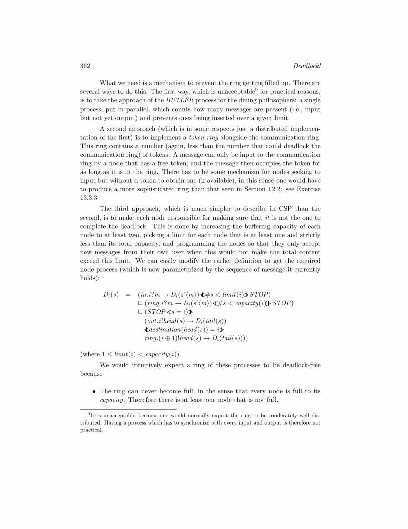
362 Deadlock!
What we need is a mechanism to prevent the ring getting filled up. There areseveral ways to do this. The first way, which is unacceptable9 for practical reasons,is to take the approach of the BUTLER process for the dining philosophers: a singleprocess, put in parallel, which counts how many messages are present (i.e., inputbut not yet output) and prevents ones being inserted over a given limit.
A second approach (which is in some respects just a distributed implemen-tation of the first) is to implement a token ring alongside the communication ring.This ring contains a number (again, less than the number that could deadlock thecommunication ring) of tokens. A message can only be input to the communicationring by a node that has a free token, and the message then occupies the token foras long as it is in the ring. There has to be some mechanism for nodes seeking toinput but without a token to obtain one (if available), in this sense one would haveto produce a more sophisticated ring than that seen in Section 12.2: see Exercise13.3.3.
The third approach, which is much simpler to describe in CSP than thesecond, is to make each node responsible for making sure that it is not the one tocomplete the deadlock. This is done by increasing the buffering capacity of eachnode to at least two, picking a limit for each node that is at least one and strictlyless than its total capacity, and programming the nodes so that they only acceptnew messages from their own user when this would not make the total contentexceed this limit. We can easily modify the earlier definition to get the requirednode process (which is now parameterized by the sequence of message it currentlyholds):
Di(s) = (in.i?m → Di(s 〈m〉)<I #s < limit(i)>I STOP) (ring .i?m → Di(s 〈m〉)<I #s < capacity(i)>I STOP) (STOP<I s = 〈〉>I
(out .i !head(s)→ Di(tail(s))<I destination(head(s)) = i>Iring .(i ⊕ 1)!head(s)→ Di(tail(s))))
(where 1 ≤ limit(i) < capacity(i)).
We would intuitively expect a ring of these processes to be deadlock-freebecause
• The ring can never become full, in the sense that every node is full to itscapacity . Therefore there is at least one node that is not full.
9It is unacceptable because one would normally expect the ring to be moderately well dis-tributed. Having a process which has to synchronize with every input and output is therefore notpractical.

13.2 Specific ways to avoid deadlock 363
• A node that is not full will accept input from its ring predecessor.
• The said predecessor can at all times either communicate with its own useror output to our node.
The crux of this argument is, of course, the first line. To turn it into a formalproof we would have to define and prove this statement, which itself requires under-standing every state the ring can reach. (One would probably go about this byformulating and proving a suitable invariant – something we will discuss later.) Wewill shortly find that the proof of deadlock freedom can be cast in rather differentterms, much more akin to the methods seen hitherto.
A substantial case study (most of which is cast in occam rather than CSP)of how this ring mechanism can be extended to a deadlock-free routeing protocolfor use on an arbitrarily connected network can be found in [103]. (End of example)
The only cycle of ungranted requests that could arise in the ring above is ofeach node blocked from outputting to its clockwise neighbour. (The reverse cycle ofeach node waiting for input does not arise because then all the nodes are preparedto input – i.e., communicate outside the vocabulary of the network, which meansthis is not formally an ungranted request.) Consider the state of an individual nodein this cycle: it is certainly full, and the last communication it performed was theone that filled it. But that communication must have been from its anticlockwiseneighbour rather than from its external user, because of the way it is defined. Wecan deduce that our node has communicated more recently with its anticlockwiseneighbour than with its clockwise one.
This brings us right back into familiar territory: as we progress clockwiseround the cycle of ungranted requests we find that the most recent communicationson the channels were earlier and earlier, creating the usual contradiction whenwe have gone all the way round. Thus the cycle, and consequently deadlock, areimpossible. This is formalized in the following.
Deadlock rule 8 Suppose V is a network which is free of strong conflict andsuch that, for each pair P ,Q of neighbouring processes, it can be shown that,whenever P =⇒•Q ,
(i) Q has previously communicated with P and
(ii) Q has done so more recently than with at least one other process to whichQ has a request,
then V is deadlock-free.
This rule allows us to prove our ring deadlock-free by local analysis (since,like all of our rules, the conditions underlying this one are checked by looking at

364 Deadlock!
the behaviour of individual processes or small collections of them). Another, largerexample that uses Rule 8 can be found in Section 15.3.1.
Of course, once we have discovered this rule, other related rules immediatelyoccur to us. We could, for example, turn the above rule around and specify thatQ must have communicated with another neighbour (to which it has a currentrequest) more recently than any communication with P . This looks less likely andthe author is not aware of any natural applications.
Exercise 13.2.1 Recall the treatment of the alternating bit protocol in Section 5.3.We argued on page 134 that it is deadlock-free. That argument can be re-cast in terms ofone of the rules in this section: do so.
Exercise 13.2.2 Suppose V is a cyclic communication network satisfying the assump-tions of Rule 5. Show how to build an ordering on the edges that satisfies the conditionsof Rule 4, showing that Rule 5 is a consquence of its predecessor. Hint: identify each edgewith the two-element set of the nodes at each end.
Exercise 13.2.3 Define a version of the ‘virtual network’ on page 350 that operates inthree dimensions rather than two. You still only require 2 layers. Define the node orderingwith respect to which Rule 2 applies to your network.
Exercise 13.2.4 Create a ring network in which the communications of each node nconsist of external events in.n.m.x and out .n.m.x , respectively meaning that the messagex is being sent to or received from node m, plus communications with the adjoining nodesof the form ring .n.p meaning that packet p is being sent to node n by its predecessor (i.e.,anti-clockwise neighbour), where p is either of the form Message.a.b.x (meaning that itcarries message x to b from a) or is Null , meaning that it carries no message. It shouldhave the effect of reliably delivering messages as addressed. Each node should basicallyhave the capacity of one packet, and should only be able to input on in when this packetis null.
The result should be a cyclic communication network that is deadlock-free by Rule4. (Note that it is only the communications with other nodes that have to follow a strictcyclic pattern and that the external inputs and outputs therefore do not.) Why are thenull packets important? (In other words, why can we not simply get away with twoconsecutive ring nodes only communicating when they have something substantive to sayto each other.)
Comment on what happens when there are no real messages passing round thesystem, so that all packets are null. What are the advantages and disadvantages of thisapproach as compared to the one in Example 13.2.5?
Exercise 13.2.5 Provide definitions of the nodes in a wormhole routeing networkbased (like that in Figure 13.4) on a two-dimensional virtual routeing network. Assumethat each message consists of a series of packets, with a special one representing the end

13.3 Variants 365
of the message. Identify which of the states of these processes are types A and B for Rule4, and check that they satisfy the necessary conditions to make this rule work.
13.3 Variants
13.3.1 Introduction
The arguments underlying the various principles in the previous section seem to bevariations on a common theme: we follow a putative cycle of ungranted requestsand find that some ordering property gives a contradiction once we have gone allthe way round.
We can unify the rules under a single theory, which gives perhaps the mostgeneral practical tool for proving deadlock freedom in networks with cycles. Theidea is related to a well-known method of proving loop termination in sequentialprogramming, namely variants. In sequential programming a variant function is ausually natural-number valued function of state, with the property that every timethe loop body is executed the value of the function decreases. The fact that such afunction cannot decrease for ever means that the loop must terminate after a finitenumber of iterations.
The corresponding idea in deadlock analysis is to make sure a variant functiondecreases round a cycle of ungranted requests. We associate a value – its variant –with the state of each process. Showing this decreases once round the cycle isenough since the variant of each process is then less than itself in the same state,which gives exactly the sort of contradiction we were getting in the arguments inthe previous section. Because this type of argument is essentially finitary, thereis no need to restrict ourselves to orders which, like the natural numbers, have noinfinite descending sequences.
The first thing we have to do to use variants is to define the functions them-selves. Usually these depend on two things: the node’s position in the network andits current trace. But there is no particular limitation on what is included – it maybe necessary, for example, to include internal process parameters or to take accountof the way an internal nondeterministic choice is resolved. All that matters is thatthe variant can be calculated in terms of the node’s own state and history.
The reason why this last condition is necessary is the requirement that thepreconditions to our proof rules are locally checkable. We need to be sure that thefact that variants decrease across ungranted requests between P and Q when weexamine their parallel composition implies that the same is true when they are partof a large network.
Given a network (Pi ,Ai) | 1 ≤ i ≤ N the associated variant functionswill usually be written fi | 1 ≤ i ≤ N . The fi are all functions into the same

366 Deadlock!
partial order Z , and as discussed above will usually be functions of the traces ofthe corresponding Pi . For clarity, many of the rules and arguments below assumethat they are functions of traces but can be modified easily to take account ofother circumstances. The objective in defining these functions is to make the valuedecrease over any ungranted request. In many – perhaps a majority of – practicalcases it is possible to make the variant decrease strictly over every ungranted request,which gives the easiest-to-understand case.
Deadlock rule 9 A network V is deadlock-free if it has a system of variantfunctions such that, for every pair (Pi ,Pj ) of neighbouring processes and everystate σ of their parallel composition
Piσ=⇒•Pj ⇒ fi(trσ Ai) > fj (trσ Aj )
Notice that we did not explicitly assume the network to be free of strongconflict: in fact the assumptions of the rule imply conflict freedom since two pro-cesses with an ungranted request to each other would both need to have variantsless than the other.
Most of the rules in the previous section can be reduced to this one. Twoexamples of this are given below, and others are included as exercises at the end ofthis section.
Example 13.3.1 (rule 4 in terms of rule 9) We can more or less translatethe proof that Rule 4 (concerning cyclic communication networks) guarantees dead-lock freedom into a system of variant functions. Notice that the proof uses two levelsof order: a cycle count and then events. This suggests that the partial order shouldcompound these two ideas together: N×L, where the first component is the naturalnumber of cycles a node has completed and the second is the linear order from thestatement of the rule. The order on this structure is
(n, a) ≤ (m, b) ⇔ n ≤ m ∨ (n = m ∧ a ≤ b)
The variant of process Pi after trace s is then just the pair (n, c) where n isthe number of cycles completed (i.e., the natural number #s div ki where ki is thenumber of events Pi communicates each cycle) and c is the channel on which it isdue to communicate on next. The statement that, for each state σ of the parallelcomposition of Pi and Pj ,
Piσ=⇒•Pj ⇒ fi(trσ Ai) > fj (trσ Aj )
then follows by exactly the arguments we put forward earlier when justifying Rule

13.3 Variants 367
4. We have simply translated the original proof to the framework of variants ratherthan found a genuinely different proof.
We can, of course, use orders (for the range of the variant functions) thatare less contrived. For example, if we enumerate the channels in the order of L:c1, c2, . . . , cM then, for sufficiently large K the variant functions
fi(s) = K × (s div ki) + nextindex (s)
work, where nextindex (s) is the index in this enumeration of the channel that Pi
is due to communicate on next. (K has to be sufficiently large so that any pair ofneighbouring processes with one a cycle behind the other always give the smallervariant to that one. M is certainly large enough.)
Slightly simpler variant functions than these can be found for many examplesof this type: see the exercises for ones that work on the matrix multiplicationexamples. (End of example)
Example 13.3.2 (rule 2 in terms of rule 9) The two things we have to buildthe variant from in Rule 2 are a node’s position in the node ordering, and what itis doing. So far as the rule is concerned there are really only two possibilities forthe latter: either it is making a request to all processes less than itself (call this anα state), or it is not making a request to any of them (a β state). There are foursorts of ungranted requests we can get in one of these networks:
1. A process in an α state can have an ungranted request to a predecessor inan α state.
2. A process in an α state can have an ungranted request to a predecessor in aβ state (because the latter is waiting for a different successor).
3. A process in an α state might (if able to output as well as input) have anungranted request to a successor in a β state.
4. A process in a β state can have an ungranted request to a successor in a β
state.
The other four cases are impossible because of the assumptions of the rule: aprocess in a β state has no requests to its predecessors, and no process can have anungranted request to a successor in an α state (here we are using the assumptionof conflict freedom from the rule).
The partial order we use is thus α, β×W , where W is the node ordering,and
• (α, x ) > (β, y) for all x and y

368 Deadlock!
• (α, x ) > (α, y) if, and only if, x > y
• (β, x ) > (β, y) if, and only if, x < y (note that the sense of the node orderingis reversed for this clause).
The variants are then obvious: a process maps to the pair of the type of its stateand its position in the node ordering. That these satisfy the requirements of Rule9 follows directly from the analysis above.
It is worth remarking that these variant functions may have to be thoughtof as functions on (maximal) failures rather than traces: in the general case it maynot be possible to tell from the trace alone whether a process is in an α or β state.(End of example)
13.3.2 Cycle-cutting sets
Having established the basic idea of a variant function, we can develop a few varia-tions which give it a little more power. The first of these is based on the realizationthat making the variant decrease strictly all the way round a cycle contains anelement of overkill. It would be just as effective if we were to guarantee the variantis non-strictly decreasing (i.e., ≥) over each ungranted request, in such a way thatthere is always at least one strict decrease in every cycle.
The easiest-to-understand way to obtain this is to nominate a set C of di-rected edges such that every proper cycle in the communication graph contains oneof them. Then we simply have to insist that ungranted requests over an edge in Calways have a strictly decreasing variant. Such a set will be called a cycle-cuttingset for obvious reasons.
As an example, consider a rectangular grid network like that defined for thematrix multiplier array earlier in this chapter. A possible C for this network is theset of all directed edges leading in any one of the four directions up, down, left orright – since any cycle is bound to contain at least one of each.
Deadlock rule 10 If the network V is free of strong conflict and has a systemof variant functions fj and a cycle-cutting set C such that, for every pair (Pi ,Pj )of neighbouring processes and every state σ of their parallel composition
Piσ=⇒•Pj ⇒ fi(trσ Ai) ≥ fj (trσ Aj ) and
fi(trσ Ai) > fj (trσ Aj ) if (i , j ) ∈ C
then V is deadlock-free.
We have had to bring in the explicit assumption of freedom from strongconflict, since the non-strict variant decrease is not enough to exclude it.

13.3 Variants 369
The more liberal requirements for variant functions can be used both tocreate simpler variants for networks that could have been dealt with by Rule 9, andto deal with some that could not. Below there is an example of each.
Example 13.3.3 (matrix multiplication again) We once again deal with thefirst – purely cyclic – array of processes defined for matrix multiplication. Chooseas C the set of downward-pointing edges. It turns out that with this choice we cansimplify the variant functions to just the cycle-count: i.e.,
fi,j (s) = #s div 4
Work previously done implies that this variant is non-increasing over all ungrantedrequests in any cyclic communication network. The important thing to notice aboutthe cyclic order we chose (guided by a linear order) – 〈up, left , right , down〉 – is thatbecause the first thing a node does on each cycle is look up, the existence of anungranted request on a downward-pointing edge (i.e., one in C ) implies that theupper node is one cycle ahead of the lower one. In other words the simplifiedvariants decrease and the conditions of Rule 10 are satisfied. (End of example)
Example 13.3.4 (binary switching network) Suppose there are a number ofpotential senders and receivers of messages, each of whom might wish to send amessage to any one of a class of receivers. With a carefully chosen network structureone can connect 2n of each with the average path length only being as long (to withina small constant factor) as that of the n2 nodes connected by a square version ofthe virtual routeing network we saw earlier.10
The network, shown for n = 3 in Figure 13.6, has 2n columns of n ‘switch’processes, with a sender and a receiver connected at each end. Each is connected toexactly one process in a different column: the one in column i and row j is connectedto the one in row k and column i j , the natural number with the same binaryrepresentation as i except that the j th least significant bit has been complemented.
The routeing algorithm is very simple: it is the duty of the processes in row jto make sure that the j th least significant bit in the address of the message matchesthat of the place it is sent to. In other words, if the (i , j ) process receives a messagefrom above, the j th bit of i is compared with that of the address. If they are thesame the message is sent down, if not it is switched across to the node’s partner(i j , j ). The path from 6 (110 in binary) to 5 (101) is illustrated in Figure 13.6.
In fact the precise nature of this routeing algorithm is irrelevant from thepoint of view of deadlock analysis, as are the contents of the messages communi-cated. Thus, we abstract away from these details. All we need concern ourselves
10Though that network certainly has compensating advantages.

370 Deadlock!
S
S
S
S
S
S
S
S
S
S
S
S
S
S
S
S
S
S
S
S
S
S
S
S
0,1
0,2
0,3
1,1
1,2
1,3 2,3
2,2
2,1 3,1
3,2
3,3 4,3
4,2
4,1 6,1
5,2
5,3 6,3
6,2
7,3
7,2
7,15,1
Figure 13.6 Binary switching network.
with is the fact that a node might receive a message from above or its partner.A message from the partner (on channel swin, say) is always sent down (channelout), while one from above (channel in) is either sent down or across to the partner(channel swout). From our point of view, under this abstraction, this latter choiceis nondeterministic.
The behaviour of a typical node is given below:
Sw = in → (Sw ′ out → Sw) swin → out → Sw
Sw ′ = swout → Sw swin → out → Sw ′
Notice that, when this process contains a message which it has decided to sendover its link (i.e., is in state Sw ′), it retains the ability to accept a message fromthe linked process. This is to avoid the strong conflict which would otherwise havearisen if both of a pair of partners decided simultaneously to relay messages to eachother. The network is free of strong conflict, but not of conflict, since when each of

13.3 Variants 371
a pair of partners is empty they have ungranted requests to each other. This lastfact implies that Rule 9 does not apply, but it is straightforward to apply Rule 10with C the set of all vertical edges (i.e., all except the ones linking partner nodes).The variant function fi,j of node Swi,j is defined:
fi,j (s) =
j when the node contains no message−j when it contains one or more messages
These work because, in our network, no node that contains a message can have anungranted request to one that is empty. Notice that when a pair of partners areeither both empty or both non-empty, their variants are equal.
The node process above is what you would get if you started with a definitionin which all the information necessary for routeing were included, and the decisionsmade accordingly, and then applied a forgetful many-to-one renaming which omittedthe address and data components of communications. This abstraction mechanismwill be re-examined in Section 13.6.1 (End of example)
13.3.3 Selective requests
The rules seen so far insist that all ungranted requests a process makes have areducing variant across them. Looking back at how we derived the FundamentalPrinciple, this is a little more than we really need. All we require is that theungranted requests which we happen to have chosen for the processes in the cyclehave this property. And of course we are free to select any ungranted request forthe process Pn in the sequence as long as it is not back to Pn−1.
In just about all the examples we have seen to date (the nearest thing to anexception among the concrete examples being the binary switching network), all therequests a process makes in any one state have been similar to each other. There wasno particular reason why the process should single one out. But in less symmetricexamples one can imagine a process might be making several very different requestsat once, and of course it (and we) might have different expectations about theprocesses at the other ends of these requests. Since we only need to follow a singlepath to find the cycle for the Fundamental Principle, it may be sensible in suchcircumstances to nominate which request to follow from a given one (selected fromthe set of requests it is making in its current state). Ordinarily one would expectto select the one (or one of those) that we are relying on eventually being able tosatisfy the request.
So as well as having a variant function of each process’s state, we will alsohave a request selector function. For each state σ of process Pi which is (i) stableand (ii) refuses all events not in the vocabulary of the network, ci(σ) must choose a

372 Deadlock!
process to which Pi has a request in σ (the assumption of busy-ness implying thereis at least one to choose from). The advantage of this is that the variant only hasto decrease across chosen ungranted requests: Pi
σ=⇒•Pj where ci(σ) = j .
We state here the rule that corresponds to Rule 9 – i.e., the variant functionsalways decrease strictly. One could similarly produce an analogue of Rule 10, butin that case care has to be taken to ensure that a pair of nodes in conflict do notselect each other.
Deadlock rule 11 If the network V has a system of variant functions such that,for every pair (Pi ,Pj ) of neighbouring processes and every state σ of their parallelcomposition
Piσ=⇒•Pj ∧ j = ci(σ) ⇒ fi(trσ Ai) > fj (trσ Aj )
then V is deadlock-free.
It is possible to modify some of the rules of Section 13.2 in the same way toallow for explicit selection, notably Rule 8 (which already contains an element ofit).
One of the best uses of selection functions is to liberalize communicationsin a network that has been carefully engineered to be deadlock-free, but where aseemingly heavy penalty has been paid for this. The approach is to extend therange of requests a process makes – adding some ‘optimistic’ ones – but in sucha way that the variant functions continue to be defined and to work for the oldrequests. The selection functions then choose the old requests.
One example of this – relaxing the constraints imposed by Rule 7 on resourceacquisition – can be found in the exercises below.
13.3.4 Weak variants
A weak set of variants is one where there is never the requirement of a strict decreaseover an ungranted request. All we insist on is a non-strict reduction. (While theremay be some use for ones equipped with selection functions as discussed above, wewill assume that this decrease occurs over all ungranted requests.) Weak variants donot in themselves prove absence of deadlocks – after all if we simply choose the sameconstant function for each process in a network, the non-decreasing requirement issatisfied whether the network deadlocks or not.
What they can do is refine our understanding of where a deadlock mightbe in a network, allowing us to concentrate our search. In some cases it may bepossible to refine the weak variants into a set that does prove deadlock freedom byone of our earlier rules, or to establish deadlock freedom by some other method. Inother words, weak variants are an analytic tool.

13.3 Variants 373
The following rule captures the main analytic principle using weak variants.
Deadlock rule 12 If the network V is free of strong conflict, and has a systemof variant functions such that for every pair (Pi ,Pj ) of neighbouring processes andevery state σ of their parallel composition
Piσ=⇒•Pj ⇒ fi(trσ Ai) ≥ fj (trσ Aj )
(a weak set of variant functions) then every deadlock state of V has a proper cycleof ungranted requests in which all the variant values are equal.
Example 13.3.5 (cyclic communication again) Good examples of the ana-lytic power of weak variants can be found in the area of cyclic communicationnetworks and, more generally,11 conflict-free networks where each process commu-nicates exactly once each cycle on each channel.
The natural weak variants for such systems are just cycle counts: in thenotation of earlier discussions of similar networks:
wi(s) = s div ki
No process can have an ungranted request to a neighbour that has completedmore cycles, because this would imply that the requesting process has communi-cated on the requested channel less times than the other process (contradicting thefact that the two processes synchronize on such events and so have at all timescommunicated on the channel exactly the same number of times).
Thus, by Rule 12, any deadlock state must contain a cycle of ungrantedrequests with every process having completed the same number of cycles. Thismeans, for example, that the fact that a process can vary its order from cycle tocycle is irrelevant: all that matters is the particular order they have chosen for thiscycle. One can, by examining how this cycle can arise, deduce that there is a cycle ofprocesses 〈Q0, . . . ,Qr−1〉 and one (with the same length) of channels 〈c0, . . . , cr−1〉where ci and ci⊕1 are both in the alphabet of Pi which insists (in the offendingcycle) on communicating ci⊕1 before ci .
If we had not already seen Rules 4, 5 and 6 we would have been in a muchbetter position to deduce them after the above analysis.
We now turn to a fascinating specific example, where we can refine the weakvariants a little. Imagine a network which behaves like the rectangular matrixmultiplication array except that nodes are allowed to choose nondeterministicallyin which order to communicate the two inputs and in which order to communicate
11The generalization comes from not assuming that the communications are in the same ordereach cycle.

374 Deadlock!
the two outputs. (We still insist that inputs precede outputs.) Ignoring the datavalues and calculations, the resulting node then behaves like
NDN = ((left → up → SKIP) (up → left → SKIP));((right → down → SKIP) (down → right → SKIP));NDN
Now consider the number of half-cycles a node has completed when it has an un-granted request to its neighbour.
• When it has an ungranted output (down or right) request it must have com-pleted at least one more half-cycle than the process it is requesting to.
• When it has an ungranted input (left or in) request it must have completedat least the number that is one less than the half-cycle count of the processit is requesting.
If we therefore define a set of weak variants
wi,j (s) = i + j + (s div 2)
we find that these satisfy the conditions of Rule 12. For a process such that i+j = K(level K ) outputs to ones at level K + 1 and inputs from ones at level K − 1.
We can thus infer that any deadlock state of the resulting network must havea cycle of nodes whose variants wi,j (s) are equal. Closer examination shows this tobe impossible, for
• If a process (in level K , say) has an ungranted request to one in level K + 1and their variants are equal (i.e., the first process has completed exactly onemore half-cycle than the second) then the second process itself has all itsungranted requests to other processes in level K . (In other words, it mustbe waiting for its other input first.)
• If a process (in level K , say) has an ungranted request to one in level K−1 andtheir variants are equal, then the second process itself has all its ungrantedrequests to other processes in level K .
• If follows that the cycle of ungranted requests lies in the nodes on two ad-joining levels: K and K + 1, say. But there is no cycle amongst these nodes(which actually form a chain when thought of as a graph).

13.3 Variants 375
In other words, from the point of view of deadlock, it actually does not matterwhat order the nodes choose to input and output in on each cycle (and they maychoose independently) so long as they make all their inputs before their outputs.
Exactly the same analysis applies when we move up to higher-dimensionalgrids of processes (e.g., three-dimensional) and allow the processes to order theirinputs and outputs nondeterministically (there being as many of each as there aredimensions). Except, that is, the very last part, for in three or more dimensions theset of processes in two consecutive layers does contain cycles, and the system canactually deadlock (see exercises). This difference between two and three dimensionsis most surprising and the fact that we can discover it so easily illustrates the powerof weak variants in focusing in on the essentials of a deadlock analysis. (End ofexample)
Exercise 13.3.1 Show that the variants
fi,j (s) = 2 × (i + j ) + #s
work for Rule 9 for the matrix multiplier array.
Exercise 13.3.2 On page 367 we showed how Rule 2 could be shown to be a conse-quence of Rule 9 by constructing a set of variant functions. Do the same thing for Rule3.
Exercise 13.3.3 Recall Exercise 13.1.3. Now design a token ring, in which a sin-gle token circulates in anti-clockwise direction, and in which nodes acquire the token bysending requests to their clockwise neighbours (either on their own behalf or in passingon requests received when they do not hold the token). Find a set of variant functions forRule 9, and a simplified set (together with a set of cycle-cutting edges) for Rule 10.
Exercise 13.3.4 (a) Show that Rule 7 (resource acquisition) can by proved via Rule9, again by defining a suitable set of variants.
(b) Use the variant functions defined in (a) and Rule 11 to liberalize Rule 7:users can be given the additional ability to acquire any resource they want at any timeprovided they follow rules about there being at least one ‘legitimate’ request in each state.Formulate these rules.
Exercise 13.3.5 Figure 13.7 shows a road layout allowing visitors to drive round amonument. Cars all enter the road at A and pass round the loop until they exit at B . Asyou can see, a pair of rocks have meant that one stretch of road is too narrow for cars topass each other: it is single lane there and two-lane elsewhere.
Code CSP processes which implement this layout, with one process per lane seg-ment with the assumption that no more than one car can occupy each with, for themoment, no other restriction on who can move forward onto the next segment on their

376 Deadlock!
B
AC
D
Figure 13.7 Road with a narrow section: see Exercise 13.3.5.
route. (Except for segment C , each should have two states, Empty and Full ; C shouldhave three states, Empty , Leftwards and Rightwards .) Show that this can lead to deadlock.
It is then decided to give out-going (i.e., rightward in our picture) cars priority overin-coming ones, in the sense that an in-coming car is not allowed to enter the single-lanesegment (C ) until segment D is empty. Modify your coding to achieve this, it will requireextra communication between C and D . Your aim should be to produce a system that isnow deadlock-free via a rigorous argument. The following is a suggested argument.
Use a set of weak variants (taking values in 0, 1) to show that, in any state with adeadlock, either all segments are empty or there is a cycle of ungranted requests involvingfull segments only. Show that the first of these is not deadlocked.
Now show that, when full, segment C can never have an ungranted request to Dnor vice-versa, and that therefore the cycle of full processes cannot arise.
How would your coding and argument be affected if there were more than onesingle lane segment (all separated by two-lane stretches)? Would it work to give in-comingtraffic priority rather than out-going?
Exercise 13.3.6 Find the deadlock discussed on page 375 that appears in a three-dimensional version of a nondeterministic input/output systolic array.
13.4 Network decomposition
Remember Rule 1, which shows how simple deadlock analysis is for tree networks.We might hope to inherit some of this simplicity in cases where the network, thoughnot a tree itself, can be decomposed into a number of components (probably nottrees themselves) which are connected to each other like a tree. Specifically, wemight hope that the proof of deadlock freedom can be broken down into a separateproof for each component.
13.4 Network decomposition 377
First, we have to decide on exactly what it means for a graph to breakdown into a number of components. There are really two sensible answers to thisquestion, both of which turn out to be relevant to decomposing deadlock analyses.For simplicity we will concentrate on the coarser factorization (i.e., the one thatdivides a network into fewer pieces), but will later indicate where the other onecould have been used.
Define a disconnecting edge to be one whose removal would disconnect thecommunication graph. Such an edge can never be part of any cycle since the restof the cycle provides an alternative path between its two ends. These edges canbe thought of as the edges of a tree whose nodes are the components they leavebehind when they are all removed. These components might be termed essentialcomponents since we hope to concentrate our deadlock analysis on these.
This gives a very pleasing decomposition of our network: if C1,C2, . . . ,Ck arethe partition of the nodes (or rather their indexes) into essential components, andA∗
1,A∗2, . . . ,A∗
k are the unions of the alphabets of the members of these components,we have
‖n
i=1(Pi ,Ai) = ‖k
i=1(P∗
i ,A∗k ) where P∗
j = ‖i∈Cj(Pi ,Ai)
is the composition of the processes in the component Cj . The communication graphof this re-construction of the network is, of course, a tree and the intersection in thealphabets of two neighbouring components is just the intersection of the alphabetsof the unique pair of processes in them that are adjacent in the original graph(across a disconnecting edge).
Since we have a tree (the network V ∗ comprising the (P∗j ,A∗
j )), the obvioushope is that we can apply Rule 1. There are two requirements of Rule 1 that weneed to be careful are satisfied:
• The new network has to be busy. In other words, the subnetworks definingthe P∗
j must all be deadlock-free. This is hardly surprising: the individualproofs of deadlock freedom for the P∗
j are just the parts our overall analysisgets factored into.
• The new network has to be free of strong conflict. This creates more of aproblem since it turns out that even if the original network V was free ofstrong conflict, V ∗ need not be. If, however, each of the (disconnecting)edges in V linking two of the P∗
j is free of conflict, then it is easy to see thatV ∗ is also free of conflict, which is of course enough.
Deadlock rule 13 If each of the essential components of the network V is freeof deadlock, and each of the disconnecting edges in V is free of conflict, then V isdeadlock-free.
378 Deadlock!
This rule is pleasingly general except for the requirement that the discon-necting edges are conflict-free. This more or less excludes the nodes at either endgetting into a state where each is waiting for some stimulus (e.g., a message packet)from the other. Its use is therefore largely restricted to cases where, either naturallyor by careful design (e.g., the introduction of to-and-fro polling across such edges),the two processes at the ends of a disconnecting edge agree which channel their nextcommunication will be on.
Of course we are still left with the problem of proving the essential compo-nents deadlock-free. It is quite likely that we will use some of the methods seenin this chapter which work by proving the non-existence of cycles of ungrantedrequests. If this is done, then the restriction that the disconnecting edges areconflict-free can be dropped.
Deadlock rule 14 If the network V is free of strong conflict, and such thatnone of the essential components can contain a cycle of ungranted requests (judgedrelative to the vocabulary of V , not those of the components) then V is deadlock-free.
This is, of course, a trivial consequence of the Fundamental Principle sincethe cycle of ungranted requests this generates must lie entirely within one of theessential components. Of our rules so far, Rules 2, 3, 4, 5, 7, 9 and 10 all excludecycles entirely.
For example, we can choose the variant functions (if Rule 9 or 10 is to beour chosen method) for the different essential components independently: there isno need for variants to decrease across disconnecting edges.
We mentioned above that there are two natural ways to decompose a network.The difference between these comes from so-called articulation points: nodes ratherthan edges whose removal would disconnect the graph. The biconnected componentsof a graph are the largest subsets of a graph such that any two different points belongto a proper cycle. In general one essential component12 may divide into severalbiconnected components: the divisions coming at articulation points like the oneshown in Figure 13.8 which belongs to three different biconnected components. Tofind out more about this, consult a book on graph theory such as [46].
Rule 14 applies if essential components are replaced by biconnected com-ponents, since any proper cycle always lies completely inside one of these (whichare the smallest regions of which this can be said). This can lead to the curioussituation where we have to define two (or even more) different variant functions fora single node: one for each biconnected component it belongs to!
Exercise 13.4.1 Suppose there are two adjacent tables of dining philosophers, each
12In graph theoretic terms essential components are termed edge biconnected components.

13.5 The limitations of local analysis 379
Articulation point
Essential component
Smaller biconnected component
Disconnecting edge
Figure 13.8 Two ways of decomposing graphs.
individually made deadlock-free as in Example 13.2.4. A pair of them (one from each table)make a pact that they will always eat at the same time: how is this situation described inCSP? Show that it does not harm deadlock freedom. What can happen if there are two,disjoint, pairs of philosophers like this?
13.5 The limitations of local analysis
Deadlock is a global phenomenon over a network and sometimes arises – or fails toarise – for extremely subtle reasons. There is probably no complete method for de-ciding whether or not a network deadlocks other than brute-force state exploration.And yet all the methods described in this chapter so far have relied entirely onlocal analysis: establishing properties of the behaviour of small collections – usuallyno more than 2 – of processes. Such methods can never hope to decide all cases,though they do seem to work in a large proportion of the examples that we humansare cunning enough to devise.
If faced with the problem of designing a network that had to be deadlock-free,you should look first to the principles already established in this chapter, includingconcepts not emphasized much such as building some of the pairs of processes sothat an ungranted request can never arise in one or both directions.
There is a rather precise sense in which all of our existing methods producenetworks that are robustly deadlock-free. It is this: all of the existing rules whichthemselves guarantee deadlock freedom (Rules 1–11) actually guarantee the strongercondition of hereditary deadlock freedom, meaning that the network and all itssubnetworks are deadlock-free.

380 Deadlock!
Full track segment
Empty track segment
Figure 13.9 A simple railway layout with two trains.
What this does mean is that there can be no hope of using them to provethe deadlock freedom of networks where one subnetwork relies on the behaviour ofother processes to prevent it reaching a deadlock state it might otherwise find itselfin. The archetypal example of this is the dining philosophers with butler we sawearlier: this is not hereditarily deadlock-free since the network can deadlock if theBUTLER process is removed.
That was a case where it was very easy to do things properly, but there areother examples where this is much harder and/or unreasonable. An example of thisis shown in Figure 13.9 which shows a picture of a small railway layout, in whicheach of the pieces of track is one-way and there are two sets of points. The rules arethat a train can only move onto an empty section of track (where, if relevant, thepoints are not against it) and that each set of points can only be switched when thesegment of track containing it is empty. Unlike some other codings of railways inthis book, the only processes in this network are the track segments, with adjoiningones communicating with each other to represent the movement of a train, ratherthan there being separate train processes.
If we happen to know that there are only two trains running round thispicture we will probably quickly come to believe it is deadlock-free. On the otherhand, it is not hereditarily deadlock-free: as soon as we look at a proper subnetworksuch as that shown in Figure 13.10 there is nothing to prevent what is left becomingfilled up with trains. We have to rely on the fact that the overall network is closedto prevent any more getting in. And this can lead to deadlocks: the configuration in

13.6 Deadlock and tools 381
Figure 13.10 A subnetwork that deadlocks.
Figure 13.10 (in which one track-segment process has been removed) is deadlockedbecause the lower ‘exit’ set of points on the small loop cannot move to let out anyof the trains that are clogging this loop.
In this particular case a substantial re-coding to make trains explicit processeswould help, but the more natural way to go is probably to prove an invariant of thenetwork (namely that the total number of trains is 2) and then use this to contradictthe existence of cycles of ungranted requests. This specific sort of invariant, whichcan be written
∑ni=1 fi(σi) = K
where fi(σi) is a function of the state σi of the ith process, can itself be establishedby local analysis: what we have to show is that each action of a single process Pi
leaves its contribution unchanged, and that each communication between a pair ofprocesses leaves their joint contribution fi(σi) + fj (σj ) invariant.
13.6 Deadlock and tools
We already know how to test a process for deadlock via refinement checking13: testit against one of the specifications
DF = a∈Σa → DF
DF = (a∈Σa → DF) SKIP
13FDR has a specific deadlock-checking function. At the time of writing all this does is toperform this refinement check; everything discussed in this section about improving the efficiencyof the said check therefore applies to the FDR deadlock check.

382 Deadlock!
depending whether or not it has the potential to terminate. When a system iswithin the scope of this type of check, this is usually the easiest way to analyze fordeadlock. It has the added advantage that none of the basic assumptions such asbusy-ness and triple-disjointness made at the start of this chapter is required. Inthe first part of this section we look at ways of bringing relatively complex networkswithin the scope of this form of checking; in the second we discuss tools whichimplement techniques more like those seen hitherto in this chapter.
13.6.1 Direct mechanical checking of deadlock freedom
The direct approach to analyzing systems for deadlock: simply testing for refinementof DF has two main drawbacks. The first, which we can do little about, is thatany check of a system on FDR requires us to define a specific network. There isno sense in which we can directly prove that a particular structure of network isdeadlock-free whatever its size. We can only attack N dining philosophers for aparticular N , not for all N at once.
The second problem is one of state-space size. Many problems of interesthave (at least in non-trivial instances) very large state-spaces and quickly get outof the range that FDR can deal with by enumerating one state at a time. Thereare two main tricks that can be used to bring a problem down to the size where itsdeadlock behaviour can be analyzed on FDR.
The first is abstraction. Usually our intended use of a network will involveit in handling data values; for example, passing messages around or processingnumbers. Certainly we would expect the values passed along channels to dependon this data. It may or may not be the case that which channels the processcommunicates on also depends on data. Good examples to consider here are thematrix multiplication nodes, where the values passed along channels depend ondata, but the choices of which channels do not, and our various routeing networks,where both the contents of messages and where they are sent depend on data (i.e.,address fields).
Assume that communication on a given channel is straightforward (specifi-cally, conflict-free). In the first case above – where the only thing that depends oninput data is output data – it is clear that the data being passed is quite irrelevantfrom the point of view of deadlock analysis. Thus, for deadlock analysis, the matrixmultiplication node process
N (x ) = up?a → left?b → right !b → down!a → N (x + a × b)
is equivalent to one with all the data values removed:
N † = up → left → right → down → N †

13.6 Deadlock and tools 383
This process of abstraction has reduced a process with an infinite state space (as-suming the values are real numbers) to one with four states.14
Now consider a node from the virtual routeing network (Section 13.2.1). Thedata it transmits is in two parts: address and message contents. We would expectto be able to abstract away from the contents field in exactly the same way, sincethe only thing that depends on what is input is the value later output in the samefield. The address field is, however, used in a crucial way to decide where (in eachcase of three options) to send the data, so we cannot eliminate that so easily.
Whether we can eliminate it at all depends on whether we believe (and this isa belief we can test using the following) that the precise choice between the availableoptions is important from the point of view of deadlock. Unless you are sure it isimportant, you should turn all the choices, made on the basis of the data you aretrying to abstract, into nondeterministic ones. Thus, the two types of node in thevirtual network will become
I † = in → I ′†
I-up→ I ′†
I-left→ I ′†
I ′† = I-right→ I †
I-down→ I †
over → I †
O† = over → O ′†
O-down→ O ′†
O-right→ O ′†
O ′† = O-left→ O†
O-up→ O†
out → O†
This abstraction procedure is one you can check: if forget is the renaming functionthat forgets whatever data values we are abstracting from channel communication(e.g., forget(in.i .j .m) = in), you should find that
I † forget(I )
In other words, every behaviour that I might make is reflected in the abstractedprocess.
14This form of abstraction – removing detail which is irrelevant to the internal operation ofcomponent processes – is very closely linked to the topic of data-independence which we will studyin Section 15.3.2.

384 Deadlock!
You should then use the processes I † and O† in place of the originals whenchecking for deadlock freedom. In this case it would work: in fact the proof ofdeadlock freedom in terms of Rule 2 works just as well for the abstracted networkas it did for the original. If it does work this guarantees deadlock freedom forthe unabstracted network. If it does not, and a deadlock is found, you have todecide whether the offending behaviour was one that the unabstracted networkcould have produced or not. Bear in mind that just because a single deadlock ofthe abstracted network could not appear in the original, this does not imply theoriginal is deadlock-free.
The formal basis of this abstraction procedure is captured in the followingrule.
Deadlock rule 15 (abstraction rule) Suppose ‘forget ’ is the function thatabstracts away the data contents of one or more conflict-free channels (each of whichis contained in each process alphabet it intersects) in the network V = (Pi ,Ai) |1 ≤ i ≤ n. Then
‖n
i=1(P†
i ,A†i ) forget(‖n
i=1(Pi ,Ai))
where (P†i ,A†
i ) = (forget(Pi), forget(Ai)). Hence if the left-hand side of the aboverefinement is deadlock-free, so is V .
Notice that we already performed the same sort of abstraction in the bi-nary switching network (page 369). It can, of course, also be applied to wormholerouteing.
The second method of making the state spaces of explicit checks manageableis the combination of hiding and compression. In the stable failures model a CSPprocess P can deadlock if and only if P \ Σ can (see Section 8.4 for technical details).This is of interest because it is generally the case that the more hiding is presentin a process definition, the more susceptible it is to hierarchical compression. Theobjective of hierarchical compression (which is discussed in more detail in SectionC.2) is to build up processes in stages, at each one trying to minimize the number ofstates in their representations. The effectiveness of this technique is demonstratedby several of the example files on the web site (see Preface).
13.6.2 Automated checking of rule-based proofs
While the methods described above frequently allow one to investigate automaticallywhether a network is deadlock-free, it will certainly sometimes occur that, evenusing compressions, addressing the state space of the entire network is too great aproblem.

13.6 Deadlock and tools 385
It is then natural to ask whether automation can help in the sort of deadlockanalysis addressed in the rest of this chapter. All of the basic conditions on networkswe have used, such as busy-ness and freedom from (strong) conflict, as well as thepreconditions to Rules 1–8, can quickly be checked for any network of finite-stateprocesses, though it sometimes requires a good deal of ingenuity to do so witha refinement checker like FDR. The reason for this problem is that in conditionsrelating to how a pair of processes evolve (such as strong conflict) it is necessaryto examine the inner workings of the pair (such as whether they have requests toeach other) as well as their outward appearance as a process. It is really better,particularly because of this need to examine how pairs evolve, to build a specializedtool for checking the preconditions for deadlock rules. This has been done by JeremyMartin, whose tool is called the Deadlock Checker.15
The later, variant-based, rules are a little more problematic to automatebecause we need some way to represent the variant function. It must be recognizedthat sometimes adding a variant function can turn a finite-state process into aninfinite-state one: this obviously happens when, as in the variants used for cycliccommunication networks, the variant has an infinite range.
Martin’s tool incorporates an additional method of analyzing for deadlockwhich is arguably very close to the concept of variant, but has the advantage ofbeing completely automatic. This is based on the State Dependency Digraph (SDD),something which is usually too unwieldy to work out by hand but which is wellwithin the scope of an automated tool even for very large networks. The SDD ofa network has one node for each state of an individual process in the network V –thus its size is the sum of the state space sizes of the component processes. It has anedge from (i , σ) (Pi in state σ) to (j , ρ) if, and only if, Pi and Pj can simultaneouslyreach σ and ρ when put in parallel and then Pi has an ungranted request to Pj .
It is possible to show that the SDD is acyclic if, and only if, there is a setof variant functions for V satisfying the preconditions of Rule 9 and such that thefunctions are all based purely on the position the processes are in their finite statemachine representations. (It should be noted that not all the variant functionsused earlier have this latter property. The exceptions are those relating to cycliccommunication networks and similar.) Thus an acyclic SDD implies deadlock free-dom. Martin’s thesis [78] and tool both contain extensions of this technique to allowSDDs to be used for proving deadlock freedom in wider classes of network such asnetworks with conflict.
Clearly any cycle of ungranted requests in the network implies the existenceof a cycle in the SDD. It is tempting to believe the reverse, but there are two reasonswhy the existence of a cycle in the SDD does not necessarily imply the possibility
15See the Bibliography for the availability of this tool.

386 Deadlock!
of a cycle of ungranted requests in V .
Firstly, just because the processes round some cycle in V can reach someassignment of states when we consider their parallel compositions pairwise does notmean that the same combination can be reached in the parallel composition of theentire network.
Secondly, and more interestingly, it is entirely possible for different states ofthe same process to appear in the same cycle in the SDD. Obviously no such cyclecan correspond to a cycle of ungranted requests. It is this possibility that generatesthe restriction above that the variant functions have to be based on the specificstates used in constructing the SDD. Clearly one can look only for those cycles thatinvolve all different processes, but this appears to be much more time consuming.
Despite these drawbacks, methods based on analyzing SDD graphs appearto be perhaps the most interesting and powerful class for building deadlock analysistools.
13.7 Notes
The definitions and results in this chapter are largely taken from the author’s paperswith Dathi and Brookes [118] and [21] together with the theses of Dathi [28] andMartin [78], as are many of the examples. These are probably the best sources topursue for further details. Earlier work on the analysis of deadlock in CSP networkscan be found in [101] and [20]. There have been various applications of this type ofanalysis, especially in the occam community, see [103, 136], for example.
The fact that tree networks are a special and easy case in deadlock analysishas been long known and it is hard to pin down where it originates. The conditionsand definitions in Section 13.1 can be thought of as an attempt to capture formallythe circumstances under which the result ‘trees are deadlock-free’ is true.
The concept of a cyclic communication network was described by Dijkstraand Scholten in [33], and Deadlock Rule 4 is essentially derived from that source.
It should be appreciated that none of the combinatorial techniques describedin this chapter is complete, in the sense of guaranteeing to establish deadlock free-dom whenever it is true. It seems almost certain that no tractable locally-basedtechnique could do this, since in general the problem of deciding whether a CSPnetwork can deadlock is NP complete. All one can hope for is that the methods wehave described, and other similar ones, are sufficient to deal with the majority ofpractical deadlock analyses. Provided one is prepared to espouse the principle dis-cussed on page 345 that we should build our systems to be inherently deadlock-freerather than adding patches later, this seems a much more reasonable desire.

13.7 Notes 387
The author hopes that the wide range of deadlock analysis techniques in thischapter will deal with many of the examples readers want to handle, and also givethem ideas about how to formulate and prove their own rules to deal with otherexamples.
2005: It has recently come to the author’s attention that the concept of con-fluent processes (namely ones where if two events are possible then performing onewill not preclude the other), which can be found in Milner’s work [82], is closelyconnected with the CCNs presented in this chapter. Furthermore, it can be shownthat both these classes of network (and any others for which a set of non-decreasingvariant functions can be found, that never decrease as a process evolves) are buffer-tolerant with respect to deadlock freedom. Namely, adding arbitrary buffering neverintroduces deadlock into them.
Example transformation
A typical transformation using algebraic laws to manipulate hiding and renamingas discussed when introducing assumption D in Section 13.1.1 is given below. Theexample considered is the parallel/hiding/renaming combination
(P >>Q) >>R
We wish to move all hiding to the outside, and all renaming on to the componentprocesses.
First we observe that the name of the channel mid used in defining >> isirrelevant, because, for any other name n (apart from left and right),
P >>Q = (P [[right ,mid/mid , right]] |left,mid|‖|mid,right |
Q [[mid , left/left ,mid ]]) \ | mid |= ((P [[right ,mid/mid , right ]] |left,mid |‖|mid ,right|
Q [[mid , left/left ,mid ]]) \ | mid |)[[n/mid ]]
= (P [[right ,n/n, right ]] |left,n|‖|n,right | P [[left ,n/n, left ]]) \ | n |
(Here the second line follows by 〈f [·]-hide-null〉, and the final one by a combinationof 〈f [·]-hide-sym〉, 〈f [·]-X ‖Y -dist〉 and 〈[[R]]-combine〉 (3.16).) Note that the last lineabove is identical to the definition of P >>Q except that the name n replaces mid .
This shows that (P >>Q) >>R can be written:
(((P [[right ,n/n, right ]] |left,n|‖|n,right |
Q [[left , n/n, left ]]) \ | n |)[[right ,mid/mid , right ]]
|left,mid |‖|mid ,right | R) \ | mid |

388 Deadlock!
This is important because it allows us to push the renaming of the inner combinationdown to P and Q (using 〈f [·]-hide-sym〉 and 〈f [·]-X ‖Y -dist〉) without changing thename of the channel hidden at the intermediate level:
(((P [[right ,n/n, right ]][[mid , right/right , mid ]] |left,n|‖|n,mid |
Q [[left , n/n, left ]][[mid , right/right ,mid ]]) \ | n |)
|left,mid |‖|mid ,right | R) \ | mid |
And equally importantly it then lets us move this intermediate-level hiding, using〈hide-X ‖Y -dist〉, to the outside since the events hidden do not intersect the alphabetof the right-hand process.
((P [[right ,n/n, right ]][[mid , right/right ,mid ]] |left,n|‖|n,mid|
Q [[left , n/n, left ]][[mid , right/right ,mid ]])
|left,mid ,n|‖|mid,right | R) \ | n | \ | mid |
Finally, we can collect all the renamings of each component, and all the hiding atthe outside, together.
((P [[right ,n/n, right ]][[mid , right/right ,mid ]] |left,n|‖|n,mid|
Q [[left , n/n, left ]][[mid , right/right ,mid ]])
|left,mid ,n|‖|mid,right | R) \ | n | \ | mid |

Chapter 14
Modelling discrete time
14.1 Introduction
All of the modelling we have done so far has been done without measuring thepassage of time. We have cared about what order events happen in, but not howlong there is between them or at what time any specific one happens. When ourcorrectness criteria are independent of time (as have been all we have seen to date, ofcourse) and our implementations do not rely on internal timing details to meet theirspecifications, this abstraction is very useful since it simplifies both the descriptionof, and reasoning about, processes. Nevertheless, it is in the nature of the sort ofinteractive systems we describe using CSP that sometimes it is desirable to be ableto reason about their timed behaviour.
There are two distinct approaches to this. The more elegant is to re-interpretthe CSP language over time, and record the exact time at which each event occurs.A trace thus consists of a series of time/event pairs rather than just events. Thisleads to a range of semantic models incorporating time, just as we have seen avariety of models for the untimed version. This theory of Timed CSP, though itsmodels are sometimes surprisingly different to those we have seen (and generallymore complex), has elegant links into the untimed theory allowing development andverification to be carried out in both. This will typically allow the developer to usethe more complex timed models only for those parts of his or her work which requireit.
There is a substantial literature on Timed CSP (see Section 14.8) and, inparticular, a textbook (by S.A. Schneider) covers it in detail. We will not, therefore,go into the details of it here.
In Timed CSP, the times associated with events are non-negative real num-bers. In other words, it adopts a dense, continuous model of time. This has an

390 Modelling discrete time
intuitive appeal, since it corresponds with the standard way in which we thinkabout measuring time. It is unfortunately true that using continuous time sub-stantially complicates the problem of automating verification and, except in veryrestricted circumstances, makes decision procedures based on state enumeration in-feasible or impossible. For continuous time adds an extra infinite dimension both tothe recording of events and to the evolving process state, and it is only by imposingsevere restrictions and using clever equivalences that this infinity can be avoided.
The most obvious alternative model of time is of an infinite series of discreteinstants, equally separated. This results in a time domain which looks like thenatural numbers, though the interval between successive beats of the drum mightbe any size, from nanoseconds (as would typically be the case for a clocked circuit)upwards. In most computer applications where all of the component processes areultimately controlled by a single clock, such as clocked VLSI or scheduler-basedsystems, a discrete clock is closer to the spirit of the system than a continuous timemodel. In any case it is often possible to give a good enough approximation to othersystems using sufficiently fine discrete models.
There is a considerable variety of ways in which we could include a discretetime model into CSP. Many of these would involve incorporating time explicitly intosemantic models, as described above for Timed CSP. The subject of this chapter,however, is how to model timed systems in ordinary, ‘untimed’ CSP by including thedrum-beat of the passage of time as an explicit event. This event is conventionallycalled tock (rather than tick since that is easily – especially on tools – confused with). All of the processes with timing constraints must synchronize on the event tock :this allows us to regulate and reason about the amount each process and the overallsystem does in given time intervals.
Advantages of this approach are:
• As we will see, it gives considerable flexibility about how to model and reasonabout timed systems.
• The human user can understand timed systems without having to learn an-other model.
• Existing tools can be applied to timed systems.
14.2 Meeting timing constraints
Having taken the decision to include the tock event in a process’s alphabet, one isforced to make detailed decisions about what its actions mean and how they occurin time. This is illustrated by a timed version of COPY . Suppose it takes one unit

14.2 Meeting timing constraints 391
of time for a data value to pass through this one-place buffer, and that a further unitof time is required between the output and the next input. The obvious definition,given this, is
TCOPY 1 = left?x → tock → right !x → tock → TCOPY 1
But there is a big difference between this process and the original COPY , becausethis one insists on performing an action each unit of time: it does not allow timeto pass until it has done something on each and every cycle. The original COPYwill wait as long as you like either to input or output. It is reasonable to saythat TCOPY 1 becomes urgent one time unit after performing any action: it insistson doing some visible action before time can progress. The correct translation ofCOPY (with the same assumptions about how long it takes for one communicationto enable another) is actually
TCOPY 2 = left?x → tock → TCOPY 2′(x ) tock → TCOPY 2
TCOPY 2′(x ) = right !x → tock → TCOPY 2 tock → TCOPY 2′(x )
since this process says that there has to be at least one time unit between inputand output events, without expressing an upper bound. The states TCOPY andTCOPY 2(x ) might be said to be idling, in that the passage of time has no effecton them.
An interesting hybrid between these processes is one which will wait to input,but not to output – it idles on input but is urgent about outputting:
TCOPY 3 = left?x → tock → right !x → tock → TCOPY 3 tock → TCOPY 3
By slight modifications one can come up with versions which expect one orother of their communications to occur within any fixed N time units, or which cannondeterministically select when (and for how long) a communication is available.
Clearly, then, we can be much more expressive about how a process behavesin this timed world than previously. This makes it possible to describe paradoxicalnetworks which must meet inconsistent timing constraints. Imagine, for example,placing TCOPY 1 in parallel with a process expressing the constraint that therecannot be more than M communications in the first N time units: TLimiter(N ,M ),where
TLimiter(n,m) = RUN <I n = 0>I((STOP<I m = 0>I ?x : Σ tock → TLimiter(n,m − 1)) tock → TLimiter(n − 1,m))

392 Modelling discrete time
If M < N then our two sets of timing requirements are inconsistent, whichmanifests itself in the combination deadlocking. This is what happens when oneputs together a combination whose timing requirements do not match, which givesus an easy way of testing for this. This situation is called a time-stop. If we can placea process like TCOPY 1 or TCOPY 3 into a system without creating a time-stop, itessentially means that the timing assumptions on the availability of communicationthat are built into these processes are consistent with the system.
As a further example to illustrate this idea, we can modify TCOPY 3 so thatit is parameterized by the channels it uses and, more importantly, by the delaybetween the input and output of a datum:
TCOPY 4(left , right ,D) = left?x → TCOPY 4′(left , right ,D ,D , x ) tock → TCOPY 4(left , right ,D)
TCOPY 4′(left , right ,D ,N , x ) = tock → TCOPY 4′(left , right ,D ,N − 1, x )<I N > 0>Iright !x → tock → TCOPY 4(left , right ,D)
Let us think about what happens if we ‘pipe’ two of these together:
TCOPY 4(a, b,D1) ‖|b,tock |
TCOPY 4(b, c,D2)
If D2 ≤ D1, all is fine: we can guarantee that the right-hand process will not beexpected to make its (n+1)th input until at least D1 + 1 time units after its nth,and it is therefore ready. On the other hand, if D2 > D1, then if (though it neednot) the left-hand process makes its second input as soon as it can, this will leadto a ‘time-stop’ when it needs to output D1 units later and the right-hand processis not ready. If, on the other hand, the environment is sufficiently slow in puttinginputs into the combination, the problem will not arise.
Notice that processes like TCOPY 4 and TLimiter(n,m) have many statesthat are neither urgent nor idling: in other words they allow tock but are notunchanged by it. It is as well to have a name for this type of state too, so wewill call them evolving. Every state of a timed system falls into one of the threecategories of urgent, idling and evolving, and it is a most helpful distinction to bearin mind when designing programs for this style of CSP system.
In most examples it would be ridiculous to have infinitely many ordinaryactions between two tocks, since this would mean that infinitely many actions occurin a finite time interval. This is equally easy to check for, all we have to do is lookfor divergence in
P \ (Σ tock)

14.2 Meeting timing constraints 393
Indeed, the most basic ‘sanity check’ on this sort of model of a timed system isto verify that the above process equals (which is equivalent, because the followingprocess is deterministic, to saying that it refines)
TOCKS = tock → TOCKS
in the failures/divergences model. This shows that infinitely many actions cannotoccur in any finite time interval, and that no matter what happens it is possible(provided the environment communicates appropriately) for time to progress – inother words, there are no reachable inconsistencies in the timing constraints. If therewere any possibility of our process terminating () we would have generalized thisto proving refinement of
TOCKS = (tock → TOCKS) SKIP
though this will never be necessary for any of the examples we deal with in thischapter.
As said above, a process can satisfy this check when, in order to let time pass,it is necessary for the environment to engage in suitable communications with theprocess. Both TCOPY 1 and TCOPY 3 satisfy it, for example. It may well be thatwe need the process to be tolerant of not receiving some or all communications in-stantly – the most obvious distinction here being between input and output events.1
(It may well be reasonable to assume that the environment is always willing toaccept an output, but it may be unreasonable to assume that the environment isalways waiting to send an input.)
If there is a set of events D which the environment is assumed to be allowed todelay indefinitely, but may still allow, the above test should be modified to showingthat
(P ‖D
ChaosD) \ (Σ tock)
refines TOCKS . If D = | left |, we will have that TCOPY 3 satisfies this but thatTCOPY 1 does not. The point is that ChaosD may either allow or prevent actionsfrom D , so the process can neither discount the occurrence of these events nor relyon them happening. Setting D equal to Σ tock would correspond to all normalevents being arbitrarily delayable by the environment – the conventional CSP viewof communication.
1There are similarities between this distinction and the one between ordinary and signal eventsdiscussed in Section 12.1.2. Indeed, the process defined here for testing timing constraints isexactly the mixed abstraction defined in that section. Setting D = Σ tock reduces it to lazyabstraction.

394 Modelling discrete time
In the above checks, using failures-divergences refinement will ensure thatonly finitely many events happen between tocks, whereas using failures refinementwould check only for time-stops. It might well be the case that you want to relaxthe condition that only finitely many events can happen between tocks, but onlyas regards delayable events. In some circumstances it may be more appropriate torely on the external process instigating these events not to send infinitely many in afinite time, and so putting in restrictions into our process P might seem unnecessaryand overcomplex. A good example of this will be found in the case study of thebully algorithm (Section 15.2). One appropriate check to use in this case is that
P \ (Σ (D ∪ tock))
failures/divergences refines
TOCKS ||| ChaosD
This says that events in D are never required to enable tock to happen, and thatonly finitely many other events happen between each pair of events that are eithertock or in D . If you intend to join a pair of processes together, with each process’ssignal events being the delayable ones of the other, then this weaker check oughtonly to be used at one end of the interface.
It would also be possible to allow for an environment that will guaranteeintermediate levels of acceptance of communication, such as guaranteeing to acceptany communication in a set B if offered for at least N units. There might well be arole for such tests when we know that the component in hand will ultimately be putin a system that makes such guarantees (because, for example, of scheduling). Butin specifying a ‘complete’ system, events will tend to come into the category thatare simply observed by the environment, which it cannot delay, and those whichthe environment can delay indefinitely.
Exercise 14.2.1 Define a version of TCOPY which outputs at a time it nondeter-ministically chooses between A and B time units from the corresponding input. It is thenready to input again C units later. What might happen when two of these are connectedtogether?
Exercise 14.2.2 Give trace specifications for the following: (i) no more than Nordinary events occur between any two tocks, (ii) no more than M tocks occur betweenconsecutive occurrences of the event a. Give definitions for the characteristic processes ofthese specifications.
Exercise 14.2.3 Recall the cash-point machine examples in Part I. Define a versionin which the machine will wait only M time units for the correct insertion of the PIN, andotherwise will retain the card. It should wait indefinitely for all its other communications.Identify which states of the system are urgent, which are idling, and which are evolving.
14.3 Case study 1: level crossing gate 395
14.3 Case study 1: level crossing gate
A level crossing is where a road crosses a railway track (without a bridge or tunnel).The road direction is usually controlled by a gate that is meant to stop cars gettingonto the railway line when a train is passing. In this example we consider a simplemodel of this, in which timing is used to establish basically untimed safety properties(e.g., when a train is near or on the gate, the gate is down) and to specify timingproperties of the system (e.g., the gate goes up within K units when there is notrain near or approaching).
We describe this system as a parallel combination consisting of a number ofparts:
• processes representing track segments;
• processes representing trains;
• processes describing timing constraints on these things;
• a process representing the gate;
• a controller process which monitors sensors, etc., and sends control signalsto the gate.
For simplicity we will model the case of a single line along which trains onlymove in one direction. The track is broken into segments (which are at least as longas any train). They are numbered, with this sensor in segment 1 and the crossingand output sensor in segment GateSeg .
We are not going to rely on timing for anything other than the properties ofthe gate. Other safety requirements obviously apply to our little system, such asthat there are never two trains on the same track segment, but these will not be ourprimary concern here. Our method of system development will be to describe thetrack segments and trains as untimed processes, and later put processes in parallelwith them to describe their timed behaviour.
The following gives an untimed description of train t on track segment j .Note that a train enters the next segment (j + 1) before it leaves segment j , andthat there is a ‘track segment’ 0 which represents the outside world. SC denotesthe number of segments including this segment 0. We will assume that the levelcrossing itself is in segment GateSeg , which lies between 1 and SC − 1. For timingreasons it should never, in fact, be either the first or last segment.2 Here, t ranges
2If it were the first then it would not be possible to get the gate down in time and if it were thelast then the way we later arrange our timing constraints means there would be no guarantee atrain would ever leave GateSeg, thus preventing the gate from rising. The best value for GateSegis probably SC − 2.

396 Modelling discrete time
over a set TRAINS of train names and ⊕ represents addition modulo SC .
Train(t , j ) = enter .t .j⊕1→ leave.t .j → Train(t , j⊕1)
The track segments can be occupied by one train at a time, and each time atrain enters segment 1 or leaves GateSeg the appropriate sensor fires.
Track(j ) = (enter?t !j → sensor .in → Trackf (t , j ))<I j = 1>I(enter?t !j → Trackf (t , j ))
Trackf (t , j ) = leave.t .j → sensor .out → Track(j )<I j = GateSeg>Ileave.t .j → Track(j )
It makes sense to consider the combination of the SC − 1 track segmentprocesses with as many trains as we wish to consider. The processes within each ofthese classes do not communicate with each other, but the collection of all trainssynchronizes with the tracks on all enter and leave events apart from those relatingto the notional ‘outside’ segment 0.
Tracks = Track(1) ||| . . . ||| Track(SC − 1)
Trains = Train(Duncan, 0) ||| . . . ||| Train(Thomas, 0)
Network = Trains ‖IFace
Tracks
where IFace = enter .t .j , leave.t .j | t ∈ TRAINS ∧ j ∈ 1 . . .SC−1
It would, of course, be possible to prove various safety properties of this system,such as the fact that there are never two trains on the same track segment.
None of these processes uses the time event tock , but since our eventual goalis to ensure via timing that the gate is up and down at appropriate moments, wehave to make some assumptions about the relative timing of the events in the abovesystem. What we do in this case is to introduce one or more timing processes toregulate the behaviour of each of the component processes that needs it.
We can make assumptions about the speed of the trains as they pass throughour system by regulating how many units of time are taken over a track segment.Let us suppose there are identifiers MinTocksPerSeg and MaxTocksPerSeg whichrepresent our assumptions about the minimum and maximum number of time unitsa train can spend per track segment. This could be expressed either as a constrainton trains or on track segments. In the former case one might set out the range oftimes a train can spend between successive enter events (in which case it is necessaryto special-case the behaviour when outside the system). In the latter case one might

14.3 Case study 1: level crossing gate 397
express a bound on the time between any train entering and leaving a segment, orbetween them entering a segment and entering the next. While the enter/leaveapproach has obvious attractions, it has the disadvantage that the length of a trainaffects how fast it can travel – presumably the enter event is triggered by the frontof the train and the leave event by the back. This would also mean that the sametocks can apply to the train’s passage through two different segments: the timetaken to pass through several would not be the sum of the times apparently takenfor the individual ones. The approach we take is therefore the first alluded toabove: expressing upper and lower speed limits on all the real track segments viaconsecutive enter events.
SpeedReg(j ) = enter?t !j → SpeedReg ′(j , 0)tock → SpeedReg(j )
SpeedReg ′(j ,n) = (tock → SpeedReg ′(j ,n+1)<I n < MaxTocksPerSeg>I STOP) (enter?t !j⊕1→ SpeedReg(j )<I n ≥ MinTocksPerSeg>I STOP)
Slight modifications would allow the speed limits to vary from segment to segment,or to change from this ‘track-centred’ constraint to a ‘train-centred’ one (with oneprocess per train).
The only other timing constraints we need are on the firing of the sensors:we specify that these must fire within one unit of a train entering the first segmentor leaving the last, as appropriate.
InSensorTiming = enter?t !1→ sensor .in → InSensorTiming tock → InSensorTiming
OutSensorTiming = leave?t !GateSeg → sensor .out → OutSensorTiming tock → OutSensorTiming
Thus we end up with timing regulators only on the track segments. Thanksto the associative properties of parallel operators, there are two equivalent ways ofadding in these constraints:
• We could rebuild the process Network by adding the timing constraints in-dividually onto the component processes before combining them together(bearing in mind that all the ones this is done to – in this case the tracksegments – need to be synchronized on tock). This approach is complicatedin our example by the fact that most SpeedReg(j )’s overlap the alphabets oftwo Track(j )’s.
• We could combine all the timing constraints together as a single process

398 Modelling discrete time
and put it in parallel (synchronizing on all relevant events) with the existingNetwork .
Using the second of these approaches, we get the additional process structure
SpeedRegs = ‖SC−1
j=1(SpeedReg(j ), αSR(j ))
where αSR(j ) = tock , enter .t .j , enter .t .j⊕1 | t ∈ TRAINS
SensorTiming = InSensorTiming ‖tock
OutSensorTiming
NetworkTiming = SpeedRegs ‖S
SensorTiming
where S = tock ∪ enter .t .1 | t ∈ TRAINS
TimedNetwork = Network ‖T
NetworkTiming
where T = leave.t .GateSeg | t ∈ TRAINS ∪ | enter , sensor |
The gate is operated by a controller process. In terms of CSP modelling, wecould either build our assumptions about the timing behaviour of the gate into thecontroller process itself, or have a separate gate process. It is probably better todo the latter, particularly if there is any nondeterminism about the gate timing.Therefore we will define separate controller and gate processes. There are then fourbasic states of the controller, some of them parameterized by a count of trains (thenumber currently in the domain).
To illustrate a different way of constructing timed processes, we include therather simple timing constraints on the operation of the controller into its basicdefinition rather than add them in later.
When the gate is up we allow time to pass or the inward sensor to fire, whichimmediately (i.e., before the next tock) causes the godown command to be sent tothe gate. The first of the four states is thus:
ControllerUp = sensor .in → gate!godown → ControllerGoingDown(1) tock → ControllerUp
This raises an interesting question about our model: what happens if the sensor .outevent occurs in state ControllerUp? Now of course we do not want this to happen,since it would mean that a train was on the segment including the crossing while thegate is up. The process above, as written, would simply refuse the sensor event –a refusal that does not really correspond to reality since simply refusing to look ata problem does not mean it is not there! There are at least three ways one couldresolve this:

14.3 Case study 1: level crossing gate 399
1. Remember that our description is not accurate in this eventuality but provelater that it never happens. (One of our aims will be to show that the gateis always down when there is a train nearby.)
2. Note that the process OutSensorTiming implies that the event in questionmust happen within one unit of time from the one that causes it, and thatthe refusal of it when possible would cause a time-stop, since the basic timingconsistency check would have failed.
3. Add a clause to the above definition of ControllerUp which accepts the event.It might then either cause an error/alarm condition or simply ignore it.
Of these, the author prefers the last since it avoids using either assumptions orthe subtleties of timing to ensure our definitions make sense. And while we canlater verify quite independently that the basic safety condition holds, it is useful fordebugging purposes explicitly to catch obvious error conditions, so we modify theabove definition to
ControllerUp = sensor .in → gate!godown → ControllerGoingDown(1) sensor .out → ERROR tock → ControllerUp
On the whole, if a process is one that simply observes an event (as the controllerobserves various sensors) rather than being able to refuse it, it is good practiceto write the definition of the process in such a way that this pattern is obviouslyadhered to.3
The two states ControllerGoingDown and ControllerDown both keep a recordof how many trains have to pass before the gate may go up. Each time the sensorevent occurs this count is increased. In order to keep the controller finite state,we put in a clause to ensure that the count should not get greater than the num-ber of trains that can legally be in the domain (which equals the number of tracksegments). The ControllerGoingDown state comes to an end when the gate.downevent occurs. It is no more legitimate for the sensor .out event to occur in this statethan the previous one, so the same solution is adopted.
ControllerGoingDown(n) = (ERROR<I n > GateSeg>Isensor .in → ControllerGoingDown(n+1)) tock → ControllerGoingDown(n) gate.down → ControllerDown(n) sensor .out → ERROR
3This is related to the concept of a monitor that was defined on page 317.

400 Modelling discrete time
When the gate is down, either sensor event may occur, incrementing or decre-menting the train count as appropriate (subject to the same finite state limitation).When there are no trains left in the system the gate is signalled to go up.
ControllerDown(n) = (ERROR<I n > GateSeg>Isensor .in → ControllerDown(n+1)) tock → ControllerDown(n) sensor .out →((gate!goup → ControllerGoingUp)<I n = 1>I ControllerDown(n−1))
When the gate is going up, the inward sensor may still fire, which means thatthe gate must be signalled to go down again. Any occurrence of the other sensorevent is an error, as previously. Of course this state may get the signal confirmingthe gate is up, and will then return to its initial state.
ControllerGoingUp = sensor .in → gate!godown → ControllerGoingDown(1) sensor .out → ERROR tock → ControllerGoingUp gate.up → ControllerUp
In the above definitions, you can take ERROR to be any process whoseactivation would make itself felt in the complete network, in the sense that it istrivial to check that it never occurs. The two obvious possibilities for ERRORare the divergent process div (which requires the full failures/divergences modelto detect it), and a process that raises an alarm via an error event (which shouldnot, of course, be synchronized with any other error events there may be in otherprocesses).
ERROR = error → STOP
If the latter approach is taken, one should assert that the error event neverappears by proving that the ultimate system refines ChaosΣ error.
Neither ERROR nor div makes any allowance for how the system behavesafter an error occurs. This is fine when, as in this case, our objective is to provethat errors never occur; but when errors can occur and have to be handled, a morecareful treatment would be required.
The gate process can always be commanded to go up or down, and will obeythe command in some nondeterministically chosen time within assumed bounds.

14.3 Case study 1: level crossing gate 401
When it reaches either the up or down state it sends a signal indicating this.
GateUp = gate.goup → GateUp gate.godown → GateGoingDown(0) tock → GateUp
GateGoingDown(n) = gate.goup → GateGoingUp(0) gate.godown → GateGoingDown(n) (((gate.down → GateDown)
tock → GateGoingDown(n+1))<I n < DownTime>I (gate.down → GateDown))
GateDown = gate.goup → GateGoingUp(0) gate.godown → GateDown tock → GateDown
GateGoingUp(n) = gate.goup → GateGoingUp(n) gate.godown → GateGoingDown(0) (((gate.up → GateUp)
tock → GateGoingUp(n+1))<I n < UpTime>I (gate.up → GateUp))
This completes the definition of the component processes, and we can nowadd the last two processes to the network:
GateAndController = ControllerUp ‖|tock ,gate|
GateUp
SYSTEM = TimedNetwork ‖|sensor ,tock |
GateAndController
It is worth noting that all the components of the system have been initializedto indicate that there are no trains in the domain and the gate is up. This is muchthe simplest (both to define and to understand) initialization, but it would bepossible to deal with other situations as long as care were taken to make sure thatall of the components were initialized consistently.
The reason why timing analysis is necessary in this system is that there isno interlock that prevents a train getting onto the level crossing when the gate isnot down: note that TimedNetwork and GateAndController only synchronize ontock and the sensor events. We are relying simply on the relative times that thetrain takes to get from being sensed, to reaching the gate, and from the firing ofthe sensor to the gate being fully down. Whether the basic safety requirement is

402 Modelling discrete time
satisfied will depend on just what parameters (number of track segments, speedlimits and gate timings) are used.
Before looking at this issue in detail we need to establish, on the patterndiscussed earlier, that the timing descriptions in our code are consistent. Most ofthe events in our system are ones which are observed by, rather than controlledby, the external environment. The only events that the system does not rely onhappening within some bound are those representing trains’ entries into segment 1.Beyond that it does make various progress assumptions. So the only events that areconsidered to be delayable by the environment are D = enter .t .1 | t ∈ TRAIN in the check that
(SYSTEM ‖D
ChaosD ) \ (Σ tock)
failures/divergences-refines TOCKS .
Given the chosen initialization, the assertion that the gate is always downwhen there is a train on the same segment as the crossing comes down to two things:
• When a train enters GateSeg , the gate is down, in that the most recent (non-tock) event communicated by the gate process is gate.down . (Note that thegate is initially up.)
• The gate never goes up when there is a train on GateSeg , in that no gateevent occurs between a train entering GateSeg and leaving it.
These are both elementary safety specifications which can be expressed as follows.Let A, B and C be disjoint sets of events. We can define a general trace speci-fication BetweenSets(A,B ,C ) stating that events in C only happen between be-ing enabled by any element of A and the next element of B (which disables C ).OutsideSets(A,B ,C ) is the same except that elements of C are initially enabled(becoming disabled by the first member of B). We define two processes representingtrace specifications of these things over the events A ∪ B ∪ C , and then lift4 these
4This is a case where we are specifying the behaviour of a process in what is potentially aproper subset of its alphabet. See Section 12.2 for alternative ways to formulate such checks.

14.3 Case study 1: level crossing gate 403
to specifications that allow other events as well.
BetweenSets ′(A,B ,C ) = ?x : A→ OutsideSets ′(A,B ,C )?x : B → BetweenSets ′(A,B ,C )
OutsideSets ′(A,B ,C ) = ?x : C → OutsideSets ′(A,B ,C )?x : A→ OutsideSets ′(A,B ,C )?x : B → BetweenSets ′(A,B ,C )
BetweenSets(A,B ,C ) = BetweenSets ′(A,B ,C ) ‖A∪B∪C
ChaosΣ
OutsideSets(A,B ,C ) = OutsideSets ′(A,B ,C ) ‖A∪B∪C
ChaosΣ
The two requirements described above can thus be formalized as specifica-tions to test for the refinement of:
EnterWhenDown = BetweenSets(gate.down,gate.up, gate.goup, gate.godown,enter .t .GateSeg | t ∈ TRAINS)
GateStillWhenTrain = OutsideSets(leave.t .GateSeg | t ∈ TRAINS,enter .t .GateSeg | t ∈ TRAINS, | gate |)
Since these are trace specifications we can take their conjunction by placingthem in parallel:
Safety = EnterWhenDown ‖ GateStillWhenTrain
Whether or not this is satisfied will depend on the timing details, as discussedabove, even though the specification itself does not mention time.
This is a safety specification in more than one sense of the word! Anothersafety, in the technical sense only, specification we might want is that the gatedoes not go down unless there is a train in the domain. The most natural way ofexpressing this one is as a pure trace property:
tr = tr ′ 〈gate.godown〉 ⇒ #(tr INS ) > #(tr OUTS )
where
INS = enter .t .1 | t ∈ TRAINSOUTS = leave.t .GateSeg | t ∈ TRAINS
This can be expressed as a process to refine, but since that process involves a countof the number of trains presently in the domain, in order to make it finite-state onehas to assume a limit (just as in the controller process).

404 Modelling discrete time
It is also possible to express safety conditions involving time, typically ex-pressing some limitation on the times certain events can happen. In the presentcase one could, for example, assert that the event gate.up only happens within acertain interval of an event of the form leave.t .GateSeg .
There are two distinct varieties of liveness conditions that appear in thissort of timed reasoning: those which assert that some set of events is offered by theprocess in appropriate circumstances (very possibly involving time in the conditions)and those that assert that things definitely occur within some time. The first sortcorresponds best to untimed liveness conditions, and we will shortly look at animportant class of these in detail. The second sort is made possible by our abilityto define urgent processes that insist on certain communications before allowing theevent tock . They are, in fact, trace conditions, since they make statements such as‘no more than three tocks occur before an output’ and depend on our model of time:we know that tocks appear regularly, so if the only way for four tocks to happen isfor an output to appear, then it does. Thus any trace condition which expresses alimit on when the event tock can occur is, in fact, a liveness condition of this secondvariety.
The following expresses a condition of this sort, namely that the gate riseswithin K units of the last train leaving unless some other train appears before thattime limit expires. Once again we express it as a pure trace condition, the sameconsiderations applying to the construction of a process-style specification as in theearlier case.
⎛⎝ ((tr = tr ′ 〈leave.t .GateSeg 〉 tr ′′)∧ (#(tr ′ INS ) = #(tr ′ OUTS ) + 1)∧ #(tr ′′ INS ) = 0 ∧ tr ′′ ↓ tock > K )
⎞⎠ =⇒ tr ′′ ↓ gate.up > 0
Again, whether or not this is satisfied will depend on the parameters. An examplefile to allow you to experiment with them for this and all the other specificationsrelating to this example can be found on the web site (see Preface).
Exercise 14.3.1 How should the system be adapted to handle two or more railwaytracks running over our crossing gate? Hint: different tracks are independent of each other,and the total number of trains present is the total of those on the individual tracks.
Exercise 14.3.2 Give the controller the responsibility of turning on and off a redtraffic light that must always be on when the gate is down and for some defined timebeforehand. You should both modify the ControllerUp process to do this, and formulateappropriate specifications for the new events used by the light.

14.4 Checking untimed properties of timed processes 405
14.4 Checking untimed properties of timed processes
It will often be the case that we want to compare a process in our timed styleagainst an untimed specification (which could be simply an untimed version of thesame process). Where the specification is of traces only, there is no real problem incomparing a timed process against it: all one has to do is modify the specificationso it ignores tock events – something we did without thinking about it several timesin the level crossing gate example and which could be done simply by hiding tock .
Divergence (except for cases where an infinite number of events appear ina finite time) is a rather different phenomenon in the timed world than in theuntimed one. In many ways it is less dangerous because of the fact that timedways of looking at processes tell you what they are doing at each moment, ratherthan only giving an accurate picture when internal activity has stopped (whichnever happens in a diverging process). It is sufficiently different that, except for thecase of infinitely many actions in a finite time, it is difficult to formulate a generalmethod for approaching the question in our timed formulation. Indeed, in manycases timed analysis can make sense of, and prove well-behaved, systems that theuntimed models would regard as divergent.
What we will concentrate on in this section is how to prove untimed failuresspecifications of timed systems. In other words, we want to place limits on whattraces a process can perform, and specify things about what the process offersafter each trace. (This is distinct from the extremely strong liveness propertiesillustrated in Section 14.3 which asserted that events were not only offered, butdefinitely happened.) The crucial issue with this type of property is deciding whatwe mean by the word ‘offer’. An untimed failure (s ,X ) means that the process canget into a state after the trace s where it can refuse X and will refuse it for everafter because it has become stable. The best timed analogue of what is intendedby an untimed failures specification that precludes a particular refusal X is that,after some time beyond the end of the trace, the process will get into a state whereit must accept an element of X , and will do so for ever after until some (non-tock)visible event occurs.
What we will in fact attempt to do in this section is to prove this statement,but with the additional demand that the (permanent) offer occurs within some fixedtime bound. For the timed model gives us ability to see how long it takes for anoffer to be made and makes it impossible to say that an offer will eventually bemade without a limit of this sort.
The specification methods we use will be developed using an example. Thisparticular example is one where the internal timing behaviour is needed to establishthat the specification is met: the corresponding untimed process would not meetthe specification.

406 Modelling discrete time
It simply consists of a pipeline of two processes, feeding data items from leftto right.
The sender process waits for an input, and then outputs it on the next timeinterval (i.e., after exactly one tock). It then waits three tocks before being able toinput again.
TS = tock → TS left?x → tock → mid !x → tock → tock → tock → TS
The receiver waits for an input, then outputs and returns to its initial stateon the next two time intervals.
TR = tock → TR mid?x → tock → right !x → tock → TR
The system is put together by synchronizing and hiding the shared datachannel and synchronizing on tock .
TIMP = (TS ‖|tock ,mid|
TR) \ | mid |
Thinking about this system, it is clear that the output must have occurredbefore three tocks have happened since the corresponding input. This is before thenext input is possible and therefore this process behaves, in an untimed sense, likethe one-place buffer COPY
COPY = left?x → right !x → COPY
even though the untimed analogues of S and R would behave like a two-place bufferif piped together. Note we are assuming that the external output is not refusableby the environment.
Since COPY is an untimed specification that does not mention tock , and ourproposed implementation is a system that certainly does communicate this event,it is clear that we cannot simply ask the question
COPY TIMP?
and expect a sensible answer. We will have to do one of two things:
• Build an understanding of time, and of our requirements for when offers needto be made, into the specification.
• Abstract away the time event tock from the implementation in an appropriateway.

14.4 Checking untimed properties of timed processes 407
In fact, either of these is possible. The obvious argument against the first isthat we have negated the objective of this section: if internal manipulation to bringtime into the specification is needed, it is no longer an untimed specification! Infact we can do better than that and one can devise rather precise recipes for doingthe check in ways that do not require internal manipulation of either the untimedspecification or the timed implementation. Since they are both quite interesting intheir own right and give insight into the problem and each other, we will describethem in the following subsections.
14.4.1 Abstracting time
We know two basic ways to abstract away from a set of events: lazy and eagerabstraction (see Chapter 12). Since the tock event is interpreted rather differentlyfrom other events, it is worth while investigating what it would mean to abstract itin these two ways.
In lazy abstraction we are placing no reliance on the abstracted events everhappening. Thus the refinement test appropriate for the use of lazy abstraction:
COPY F (TIMP ‖tock
Chaostock) \ tock
asserts that the process TIMP does what is required of it by COPY no matter howmany tocks it has done. In particular, it can never refuse whatever event COPYsays it must accept next, no matter how short a time has passed since the lastaction. Clearly, then, this refinement does not hold because our system takes sometime before it is able to move from one communication to the next.
In eager abstraction, where the corresponding check would be
COPY FD TIMP \ tock
we are assuming that the abstracted events are never resisted by the environment.While this is true (hopefully) of the tock event, the different interpretation we makeof this event means that eager abstraction’s consequences for failures refinementtesting are wrong. For any process which can let time pass indefinitely (i.e., com-municate infinitely many tocks without other intervening communication) will giverise to divergence under this form of abstraction (which is just hiding) so that noassertion can be made about what the process accepts or refuses between thesetocks. In other words, eager abstraction will only pick up refusal information whenand if the process has run out of tocks to perform.
What we want to achieve is a mixture of the two. We want to allow a fixedinterval to pass during which the process can offer what it likes, but after that we

408 Modelling discrete time
want to specify what it must offer irrespective of whether it can perform anothertock . We need to apply eager abstraction to the first few tocks after an event, andlazy abstraction to the rest.
A certain amount of subterfuge is required to achieve this hybrid abstraction(which is not the same as the mixed abstraction used in Chapter 12). We employthe ideas introduced on page 3.2.3 to differentiate between identically-names eventsvia one-to-many renaming and parallel composition. We transform the timed im-plementation process by allowing either of two sorts of tock events when the originalcommunicates the original one:
RTIMP = TIMP [[tock1, tock2/tock , tock ]]
Having got two sorts of tock , we then constrain the process so that exactly one ofthem is possible whenever the original process can perform a tock . Specifically, thefirst N after the start of time or a non-tock event become tock1’s while the restbecome tock2’s.
REG(n) = nontock → REG(N ) (tock2→ REG(n)<I n = 0>I tock1→ REG(n−1))
Reg = REG(N )[[x/nontock | x ∈ Σ tock , tock1, tock2]]
RegTIMP = RTIMP ‖Σ
Reg
The effect of this complex procedure is to give the classes of tock ’s that wewant to treat differently different names. We can therefore apply eager abstractionto the tock1’s and lazy to the tock2’s to get the effect we want. The appropriatetest is then
COPY F (RegTIMP ‖tock2
Chaostock2) \ tock1, tock2
This establishes that the refusal of the implementation process is correctwhen either (i) at least N time units have passed either from the beginning or thelast non-tock event or (ii) the process insists on a communication before allowingtime to pass. In general, increasing N weakens this test, and decreasing it until itfails will reveal the longest time one might have to wait before the underlying timedprocess is ready to accept whatever is required by the specification.
A larger example of this technique can be found in Section 14.5. Note the useof one-to-many (actually one-to-two) renaming here; as ever a very powerful toolfor achieving interesting effects when combined with a parallel regulator process.

14.4 Checking untimed properties of timed processes 409
14.4.2 Untimed specifications in a timed harness
In the first method we essentially put a harness around the implementation whichunderstood the timing requirements we were putting on the process, and did ap-propriate things to tock events to allow for these. We will now deal with thedual approach: putting a similar harness round the untimed specification so as totransform it into one which allows for the occurrence of tock and makes the samestatement about the relationship between the untimed specification and the timedimplementation as was made by the first method.
The check set out above in terms of the first method seeks to establish thefollowing:
• The untimed traces of the implementation are correct.
• If it is within N time units of the last non-time event or the start, theneither time can pass or the set of events offered by the specification meetsthe current requirements of the untimed specification.
• If at least N time units have passed then the set of events offered meets theserequirements whether time can pass further or not.
This careful statement takes account of the fact that our processes sometimes insiston communicating before tock occurs. What we will do is construct a processSpecReg which, put in parallel with any untimed specification (synchronizing on allnon-tock events), transforms it so that it says the above:
SpecReg = RSpec(N ,N )[[x/anyother | x ∈ (Σ tock)]], where
RSpec(M , r) = (tock → RSpec(M , r − 1) anyother → RSpec(M ,M ))<I r > 0>I(anyother → RSpec(M ,M )) (STOP tock → RSpec(M , 0))
We can now ‘lift’ our untimed specification to a timed one by putting this processin parallel with it:
TSpec = SpecReg ‖Σ tock
Spec
(where Spec = COPY in the example we are considering). This achieves the goalsset out above since SpecReg allows any trace of Spec with arbitrary insertions of tock ,and when RSpec offers anyother the renamed version SpecReg offers all non-tockevents and hence TSpec offers whatever of these events that Spec does.

410 Modelling discrete time
The refinement check TSpec F System makes exactly the same statementabout System as the check developed using abstraction in the previous section. Thissecond version is easier to implement, since the amount of process transformationis less, but arguably required a closer understanding of exactly what we wanted tosay about such things as the passage of time.
One possible reason for proving an untimed specification UTS of a timedprocess TC is because you want to include it as a component in an otherwiseuntimed system. It would then be natural to develop the untimed system with thespecification in the place of TC , before developing TC to meet UTS in the sensediscussed in this section. One important thing that should be borne in mind if youdo this is that we have here considered processes to meet untimed specifications eventhough they may place upper time bounds on when some visible communicationsoccur: for example the outputs of the buffers above must happen within one timeunit even though the untimed COPY process would wait. It is therefore necessaryto perform a second check on the process TC which is developed to fill the slot leftby UTS : any event of its interface with the rest of the system, which you are nottotally confident will never be delayed, must be included in the Delayable set for atiming consistency check on TC .
Exercise 14.4.1 Modify SpecReg so that it never refuses tock , but otherwise behavesas before. Comment on how the revised timed specification it produces (when combinedwith an untimed one) is relevant to the discussion above about TC and UTS . How wouldthe TIMP process above fare when checked against it?
Exercise 14.4.2 The example in this section shows how what is apparently a two-place buffer might become a one-place one thanks to timing. Find an example of anapparently deadlocking system which is deadlock-free because of timing.
14.5 Case study 2: the alternating bit protocol
In this section we give a slightly larger example of the sort of reasoning introducedin the previous section, namely proving what are largely untimed specifications ofa system which depends on timing for its correct functioning. This is a versionof the alternating bit protocol which relies on time-outs to decide when it resendsmessages and acknowledgements, rather than the mechanisms described in Section5.3.
The overall specification we want it to satisfy will still be the same, namelythat it is a one-place buffer.
Unlike the untimed example, this version does not rely on the eventual correcttransmission of data to avoid CSP divergence, but we do need some bound on the
14.5 Case study 2: the alternating bit protocol 411
loss if we are to prove that data does eventually get through, and how long this takes.Rather than make the occurrence of error ’s explicitly nondeterministic as in theearlier treatments of communications protocols, here we use the more sophisticatedcoding where error ’s are prompted by external actions as discussed in Chapter 12.This has the advantage that the limits on errors do not have to be coded into thebasic system definition, and we can thus construct a single system and analyze itunder a variety of assumptions rather than having to reconstruct the system eachtime. The only error modelled here is message loss; duplication could easily beadded.
TE = a?tag?data → tock → (b!tag !data → TE error → TE ) tock → TE
TF = c?tag → tock → (d !tag → TF error → TF ) tock → TF
Note that we have specified that all messages take precisely one unit of timeto get through and that an arbitrary time then passes before the next input. Clearlyone could make this more nondeterministic. Also, the fact that the outputs havebeen made urgent imposes the obligation on us to ensure that the processes receivingthese outputs never refuse them when offered.
The implementation of the protocol consists of a sender process and receiverprocess, linked by E and F above.
14.5.1 Describing time-outs
The crucial feature of the sender and receiver processes in this presentation is theiruse of time-outs. A time-out is a sort of choice operator between two processes(like and ), that only fully makes sense in a timed model. A time-out gives oneprocess the chance to communicate for some length of time (which is a parameterto the time-out operator) and then, if no such communication has occurred, givesup and behaves like the other process. In Timed CSP it is written
P t Q
meaning the process which times-out to Q if P has not communicated within t timeunits. It looks very like the untimed operator P Q that we have seen from timeto time, since in its most natural implementation the latter essentially behaves likea time-out though without the control over exactly when the decision to time-outis made.
In the style of CSP discussed in this chapter we will obviously have to tie theoccurrence of time-outs to the tock event. Unless we are thinking that tock has some

412 Modelling discrete time
real existence, like a broadcast clock signal, it is better not to make the time-out(i.e., the transition from P to Q) occur precisely at some tock (counted, presumably,from when the time-out combination was started). This would create a potentialsynchronization between time-outs in different parallel processes when there is nomechanism to achieve it. As a simple example, consider P t Q ‖ Q t P ,where P = a → P and Q = b → Q . If the time-outs are triggered by the sametock , this combination is certain to deadlock while, assuming that in reality theyare managed by unsynchronized clocks, we would have the possibility (though notthe certainty) of being able to communicate one of a or b for a short interval.
It is usually preferable, therefore, to specify an interval (amongst the tocks)during which a time-out will occur, without forcing it to occur at a tock. Thus atime-out will be an event whose occurrence is tied to a specific interval, very likemany of the other events we have seen in this chapter.
Perhaps the most elegant way of achieving this is to delegate the firing of thetime-out to a separate parallel process which, rather like a kitchen timer, can be setup to ‘ring’ at a given time in the future. In general the time-out controller processmight, like the more sophisticated kitchen timers,5 be programmable with a varietyof intervals. It should therefore have an input channel setup over which this datais communicated, an event it communicates back when it fires, plus the tock event.Because any time-out is abandoned if the left-hand process communicates beforethe set time, the time-out controller has to be programmed so that it can be reset.
TOC = setup?n → Armed(n) tock → TOC reset → TOC
Armed(n) = ((timesout → TOC )<I n = 0>I (tock → Armed(n − 1))) reset → TOC
The main process then sends TOC the setup signal to arm the time-out function,and includes the event timesout amongst the choices it offers during the period whilethe time-out might fire. It is combined with the TOC process (of which there is onefor every separate component that needs one, since it is possible for the network tohave more than one time-out running at once) with the setup and timesout eventshidden.
5Ones that are not egg timers!

14.5 Case study 2: the alternating bit protocol 413
The structure of the complete process is then either
(Main ‖Σ
TOC [[a/reset | a ∈ R]]) \ | setup, timesout | or
(Main ‖Σ tock
TOC [[a/reset | a ∈ R]]) \ | setup, timesout |
where R = Σ tock , setup, timesout
depending on whether or not (respectively) the process Main is timed.
For example, if P and Q are the processes described earlier when discussingthe consequences of synchronized time-outs, we can describe P t Q by definingMain (in the first line above) to be setup.t → (S ||| RUN tock), where
S = timesout → Q P
(This is a timed process because it insists on sending the setup.t signal immediately –before any tocks. The subsequent interleaving with RUN tock means there are nofurther timing constraints apart from the ones introduced by TOC .)
If Q t P is defined similarly, it is now possible for
P t Q ‖ Q t P
to synchronize on either a or b between tocks number t and t + 1.
14.5.2 The sender and receiver
In this treatment of the alternating bit protocol we have factored the sender processinto three parallel components: one for transmitting data, one for managing thetime-outs for retransmissions, and one for receiving acknowledgement signals andfiltering out repeats. By doing this it is easier to ensure that signals are sent andreceived at appropriate times. It is, of course, possible to do the same thing with asequential process: see Exercise 14.5.1.
Send(bit) = left?x → tock → Snd1(bit , x ) tock → Send(bit)
Snd1(bit , x ) = a!bit !x → setup!sto → Snd2(bit , x )
Snd2(bit , x ) = timesout → Snd1(bit , x ) tock → Snd2(bit , x ) ack → Send(1−bit)

414 Modelling discrete time
sto is a constant defining how long the process waits between successiveoutputs of the same piece of data. The following process sends the ack signal justwhen it gets each new, rather than repeated, acknowledgement on channel d .
SAck(bit) = d .bit → ack → SAck(1−bit) d .(1−bit)→ SAck(bit) tock → SAck(bit)
Note below that this ack event is used to reset the time-out timer.
SEND = ((Send(0) ‖tock ,ack
SAck(0))
‖A
TOC [[ack/reset]]) \ | ack , setup, timesout |
where A = | tock , setup, ack , timesout |
The receiver has one main component plus a timer, which is only reset (nowexplicitly) when a new (rather than repeat) input is received. In this sense itsbehaviour is not a classic time-out, since there are events the main process doesthat do not reset the timer. (This illustrates the flexibility of this approach ofusing parallel timers.) rto is the interval between successive sendings of the sameacknowledgement. Note that, in both the sender and receiver processes, it is onlyelapsed time which determines how many times each message and acknowledgementare sent.
Rec(bit) = b?tag?data →(reset → tock → right !data → c!bit →setup!rto → Rec(1−bit)<I tag = bit>IRec(bit)) timesout → c!(1−bit)→ setup!rto → Rec(bit) tock → Rec(bit)
REC = (Rec(0) ‖|tock∪αTOC
TOC ) \ αTOC
where αTOC = | setup, timesout , resetTABP = SEND ‖
|a,d,tock |((TE ‖
tockTF ) ‖
|b,c,tock |REC ) \ | a, b, c, d |
Aside from tock , the external alphabet of this system is | left , right , error |.Of these events we are relying on the environment accepting the system’s outputs(on right) promptly. Therefore the timing consistency check deems the delayable

14.5 Case study 2: the alternating bit protocol 415
events to be the complement of this set. It is appropriate to include the event errorin this set since not to do so would mean that we could not exclude the possibilitythat the process is relying on some error ’s happening to ensure correct behaviour!(Essentially we are lazily abstracting the error events, as recommended in Section12.3.)
D = | left , error |TimingConsistency = (TABP ‖
DChaosD ) \ (Σ tock)
As ever, this check simply shows there are no contradictory timing require-ments in our system. The main check, that our system behaves like a one-placebuffer, follows the pattern set out in the previous section. The checks set out belowattempt to show that the system meets the untimed specification COPY with allrequired communications being offered within a specified number of time units sincethe last external communication.
With Reg defined as on page 408:
RTIMP = TABP [[tock1, tock2/tock , tock ]]
RegTIMP = RTIMP ‖ Reg
This can now be checked against COPY by eagerly abstracting tock1 andlazily abstracting tock2 and error :
RHS = (RegTIMP ‖tock2,error
Chaostock2,error) \ tock1, tock2, error
This check, if successful (which depends on the timing parameters used), showssomething quite interesting because of the way it deals with errors. Since theprocess Reg (which chooses between tock1’s and tock2’s) allows an error event toreset its clock, what we are showing is that the offers required by COPY are madeby the time that a fixed interval has passed since the last input or output, and thelast error. This is the advantage of keeping the errors visible: we allow any numberof errors but only insist that the system makes progress when there have not beenany errors recently. If the thing which decides whether or not errors occur was aninvisible nondeterministic choice operator, there is no way such a statement couldbe made.
Having put the system together in such a way as to leave errors (or, at least,events that give us control over when these happen) visible, one can, if one chooses,make assumptions about the error rate and see what effect this has on systemperformance. The typical assumption it might be appropriate to make would be

416 Modelling discrete time
‘there are no more than L errors in any T time units’: something it is easy to specifyusing the tock style of CSP. If L = 1 we can define
ER1(T ) = ER′1(T , 0), where
ER′1(T , j ) = tock → ER′
1(T , j−1)<I j > 0>I(tock → ER′
1(T , 0) (STOP error → ER′1(T ,T )))
and ERL+1(T ) = ERL(T ) ‖tock
ER1(T ). (This definition has a lot in common with
that of Limit on page 317.) The last line in the definition of ER′1(T , j ) includes the
nondeterministic choice between error and STOP because we do not want processesto be able to rely on errors happening.
The appropriate thing to do with one of these assumptions is to use it toconstrain TABP and then to hide the error event.
CSYSTEM = (TABP ‖tock ,error
ERL(T )) \ error
One would then seek to prove that CSYSTEM meets the untimed specificationCOPY using the same methods as above, though this time there is no need to putin the abstraction of error and the fact that error has already been hidden meansthat it does not reset the specification clock. One would expect to find that thetime one needs to wait before this version of the system makes the offers requiredof it will be longer than in the version where error is allowed to reset the waitingperiod for this, and also that there would be critical error rates beyond which no‘settle time’ is long enough because there are enough errors to prevent real progress.
When this check succeeds it establishes that, provided the error pattern iswithin the limits specified, the system meets the specification in a way independentof exactly when the errors happen. This shows how one can elegantly extend totimed systems the concepts of fault tolerance described in Chapter 12. Thus, onemight prove that, provided there are no more than L errors every T time units, thesystem meets the COPY specification with settle-time (since the last proper inputor output) of N units.
Exercise 14.5.1 Write an alternative version of Send(bit) that does not require thespecial acknowledgement handler SAck(bit) in parallel with it (though it should still useTOC to handle its time-outs). Be careful that, whenever TOC wants to perform the eventtimesout , your Send does not deadlock it.
Exercise 14.5.2 Use the time-out mechanism provided by TOC to re-work youranswer to Exercise 14.2.3. Then produce a further version where the TOC is also used toplace limits on the time the user has to perform each of his or her other actions.

14.6 Urgency and priority 417
14.6 Urgency and priority
Recall the process TCOPY 2, the timed version of COPY from the start of thischapter that behaves most like the original. It will wait indefinitely for either aninput or an output. Now, preferably without looking ahead in this text, think howyou would expect the result of piping two copies of this together to behave:
(TCOPY 2[[mid/right]] ‖|mid,tock |
TCOPY 2[[mid/left ]]) \ | mid |
The issue you have to decide is: when does the hidden communication on midhappen? One time unit after the corresponding input by the left-hand process,both processes (assuming the right-hand one is not full) are willing and able to dothis action, but are also able to wait. A hidden action is one that the environmenthas no control over, so the implementation (and our modelling) has to decide whichroute to follow.
In all the timed examples seen so far we have carefully avoided this ambiguity.Whenever a hidden communication occurred between two parallel processes, one ofthem (invariably the one doing the ‘outputting’) specified exactly when it happened.This puts us under the obligation to ensure that these communications are acceptedat precisely the specified moments, for otherwise the TimingConsistency checks fail.
In reasoning about untimed CSP we made the assumption that when a pro-cess had a hidden action (a τ ) available then the τ always happens unless someother action occurs quickly. Certainly the process could not wait for ever in a statewith a τ available. The problem we have to face in modelling the passage of timeby tock events is that the untimed models of CSP do not understand the specialnature of this event. They would model the system of two TCOPY 2’s shown abovein such a way that the hidden mid event can nondeterministically happen after anynumber of tocks or never, in the sense that the infinite trace
〈left .0, tock , tock , tock , . . .〉
is possible without the transfer on mid occurring. Thus, this attempt at modellinga timed system in untimed CSP fails in an important way to model accurately ourunderstanding of how this system ought to behave.
Imagine the state this system is in one time unit after the input event left .0(which we can assume is the first event the combination does). The internal commu-nication (mid .0) is available; if it does not happen before the next tock then, unlesswe are to keep some timer running, the state the system is in after the tock is iden-tical to that before it. This means that if one tock is possible then, without specialtreatment, it must be possible for there to be any finite number before the hiddenaction occurs, and even for the hidden action never to happen at all. This would

418 Modelling discrete time
mean that the interpretation we were putting on this internal event in this worldof tocks would be different to the usual untimed models, where we have assumedthat a process cannot sit waiting for ever when there is an internal action possible.The cleanest solution to this problem is to assert that a tock never happens whenthere is an internal event available. In other words, internal events are urgent inthe sense that time does not pass when they are enabled. (Note that this mirrorsprecisely the concept of an urgent state that we have already discussed.) This isoften called the assumption of maximal progress and is common across a variety ofmodels of timed concurrency, including conventional Timed CSP.
Looking at a timed system in this way gives a (possibly strict) refinement ofthe way we would interpret it over the usual models of CSP, thinking of tock as anyother event. This is because these models (in particular the failures/divergences one)allow the implementation to choose internal events that are available in preferenceto any or all others (including tock), while our new view simply asserts that in somecircumstances it is obliged to do this.
It is perfectly clear how to simulate a system running under these new rules:we have to give internal events priority over tock . (Other events are not affectedby this.) In terms of operational semantics, what we are doing is describing a newtransition rule x−→T in terms of the old one x−→: here T is a set of time-like actions(usually tock). Unless x ∈ T we have
P x−→T Q ⇔ P x−→ Q
If x ∈ T , then
P x−→T Q ⇔ P x−→ Q ∧ ¬∃Q ′.P τ−→ Q ′ ∨ P −→ Q ′
Here, τ is the usual internal action we are familiar with.
The consequences of this re-interpretation for our system of two TCOPY 2’sis that the data moves across as soon as both sides are willing, namely, one timeunit after the later of the corresponding input and the output of the previous datum(if any) by the right-hand process.
In almost all circumstances this new, prioritized, view is the right way oflooking at timed systems and the cases where the conventional semantics providesthe right answer (like all those in previous sections of this chapter) are writtenso that the above rules are, to all intents and purposes, followed by the standardtransition rule x−→ without the need to impose them. In other words, in those casesthe semantic values of the standard and prioritized views coincide.
As discussed above, this will be true whenever one of the participants in eachinternal action is unwilling to let time pass until it has occurred. Fortunately, since

14.6 Urgency and priority 419
the new prioritized view always gives a refinement of the old one, checking a timedsystem against a specification6 will never give a false positive.
14.6.1 Consequences for semantic models
While the prioritized view of time is easy to understand in terms of operationalsemantics, it presents rather more difficulties if you want to get a denotational theoryfor predicting process behaviour (like the traces model, or the failures/divergencesmodel). The problem is that our usual models conceal all details of internal τ
actions, so there is no way of imposing the new interpretation on a process once wehave reduced it to its description in one of them. Whole new models, giving muchmore detail about what was refused by a process during a trace as well as after it,are required. While these are interesting, they are also complex and this is not theplace to describe them. The issues which arise are essentially the same as those asin modelling (continuously) Timed CSP, and there is extensive discussion of thesein the literature.
It is possible, under the prioritized view, to have two processes that areequivalent in all the denotational models of untimed CSP which are inequivalentwhen put in a simple CSP context. What this means from a practical point of viewis that the compression functions described in Section C.2 are unsafe for prioritizedanalysis, and that techniques for proving properties of processes by putting themin contexts should be considered carefully before use. Basically, you should regardthe primary means of understanding a prioritized program as being its operationalsemantics, rather than the denotational models which dominate for the standardinterpretation.
We need to understand how this new prioritized view interacts with themethods described in Section 14.4 for proving a timed process meets an untimedspecification. The answer is very simple: the first method creates problems becauseof the way time is abstracted by hiding. The problem is that once one hides a tockevent, it becomes a τ and so is put into precisely the category of events we are givingpriority to over tocks. Thus, once this hiding is done, we have lost the mechanismto impose priority of more normal τ ’s over the passage of time. Thus this methodshould not be used for systems with priority.
On the other hand, the second method, where the specification was trans-formed and the implementation left unaltered, creates no problems and should beused in preference.
The lazy abstraction of error events in this type of analysis does not appear
6Necessarily a specification that does not depend on the prioritized interpretation of time todeduce its own behaviour.

420 Modelling discrete time
to cause any problems since, by construction, it allows the abstracted events to berefused at any time.
14.7 Tools
The style of CSP presented in this chapter was developed specifically to meet thedemand for a mechanism for analyzing timed systems with FDR. Probably becauseof the practical importance of timing analysis it has become widely used for thatpurpose. A larger case study of the automated analysis of a timed system can befound in Section 15.2.
Except where priority is required, no special considerations apply to usingtools. The main thing anyone intending to use CSP tools for timing analysis shoulddo is get a good grasp of the principles of modelling time set out in this chapter.
It is possible7 to add an operator prioritize(P) to FDR as a functionapplied to processes: the process the function is applied to is given a revised opera-tional semantics of the sort described above.
Potential users of the prioritized implementation of timing are warned toensure they understand just what this construction achieves and the limitations onwhen it is safe to use it.
All the examples in this chapter, plus further examples of the style of CSPit describes, can be found on the associated web site.
14.8 Notes
As we have said previously, the techniques presented in this chapter are not TimedCSP in the sense described in the work of the author, Reed, Schneider, Davies andothers [29, 30, 31, 97, 98, 99, 127] because we do not use the continuous time modelused there. It has more in common, in terms of timing, with work on other flavoursof timed copncurrency. A good survey can be found in [3], and the rest of the papersin that conference proceedings are also useful. The primary reason for advocatingthe discrete approach here is pragmatic: while it is not as mathematically elegant,it is easier to automate its analysis and, in many respects, easier to program in.David Jackson has played an important role in the development of the style and inpromoting it.
There have been several papers published applying the tock-timed style ofCSP [14, 49], but no widely available general introductions to this style before. The
7This operator was present in later versions of FDR1. At the time of writing it has not yetbeen included in FDR2.

14.8 Notes 421
level crossing example was originally proposed in [69] and was the example used in[49].
2005: The style of CSP presented in this chapter remains widely used. JoelOuaknine [88] proved the existence of unexpectedly close links between a variant onit and (continuous) Timed CSP in his thesis. Recently the theory of informationflow presented in Chapter 12 has been extended to tock-CSP and there has beeninteresting work on semantic models for the priority model by Ouaknine and Lowe.The priority model is now supported by FDR.


Chapter 15
Case studies
We have already seen some moderately large examples of systems described andspecified in CSP in relation to protocols (Chapter 5), information flow (Chapter12), deadlock (Chapter 13) and timing (Chapter 14). In this chapter we look atsome more which illustrate some different ideas and methods, and the notation’spower in a wide variety of applications, some of which are by no means obvious atfirst sight.
All of the examples in this chapter are drawn from case studies developedas applications of FDR by the author and his colleagues. The definitions of morerealistically-sized processes such as those we use here are often easier to read inthe ASCII-based syntax used by FDR with its slightly lower emphasis on ‘alge-braic’ constructs. This syntax also helps in presenting the functional programs1
for manipulating data which form a vital part of most realistic FDR examples and,hopefully, will assist the reader to get used to the machine-readable version of thelanguage (details of which can be found in Appendix B).
In each case all the process definitions are included in the text, as are suf-ficient subsidiary definitions to make these clear and to show what is involved insetting up a realistic system description in CSP. Copies of the complete files fromwhich they are drawn are obtainable on the Internet (see Preface). Where possible,readers are encouraged to run these files in conjunction with studying this chapter.
The author hopes that readers will gain both ideas and confidence in theexpressive power of CSP from looking at these examples.
1These programs are frequently simple and self-explanatory, as the ones in this chapter hopefullyare. However, an understanding of functional programming such as can be obtained from [11] isundoubtedly useful for dealing with some types of example using FDR.

424 Case studies
Figure 15.1 Peg solitaire.
15.1 Combinatorial systems: rules and tactics
CSP can be used to describe systems quite unlike the obvious applications to net-works of communicating parallel processes. There are a great many types of systemwhich evolve according to rules based on their states’ structures and where there isa designated set of states which either one wishes to prove unreachable, or perhapsone is simply interested in finding out whether the set is reachable and if so how.An example of the former might be a railway signalling system, where we wouldhope to prove that, provided some set of rules were applied, no two trains end upon the same segment of track (amongst other properties of a similar flavour).
Examples of the latter are provided by the class of puzzles where the objectiveis to reach one of a set of target states (frequently this set has only one member)from a fixed starting state. The example we use in this section is one of the best-known puzzles of this sort: peg solitaire. The starting position of the usual versionof this puzzle is shown in Figure 15.1. Thus initially there are 32 slots with a pegin, plus an empty slot in the middle.
The rules are very simple: in any one of the four horizontal and verticaldirections (up, down, left, right) you can hop any peg over another peg into anempty slot, after which you remove the hopped-over peg. The objective is to remove

15.1 Combinatorial systems: rules and tactics 425
all but one of the pegs and leave the remaining one in the slot that was initiallyempty. Most human beings find this a very difficult puzzle.
Evidently the initial configuration can be varied, thus creating an infinity ofdifferent puzzles, some of which are soluble and some of which are not.2 The CSPscript on which this section is based supports a simple notation which allows theuser to design his or her own puzzles and try them out.
This is done by writing each puzzle as a rectangular list of lists (i.e., a list ofrows) in which the standard version is shown
Board = <<X,X,P,P,P,X,X>,
<X,X,P,P,P,X,X>,
<P,P,P,P,P,P,P>,
<P,P,P,E,P,P,P>,
<P,P,P,P,P,P,P>,
<X,X,P,P,P,X,X>,
<X,X,P,P,P,X,X>>
Here, X is a non-slot (there just to fill up the rectangle), P is a slot with apeg and E is an empty slot. (These are members of a data type which is declaredin the script.)
The rest of the script just compiles a parallel network out of the abovenotation. To do this we need the dimensions of the board:
Height = #Board
Width = #(head(Board))
and a function which extracts the value of the (i , j )th member of the array. Thefollowing definition allows for the fact that the above picture is inverted becausethe 0th row is at the top, whereas it is easier to think of the origin (point (0, 0)) asbeing at the bottom left-hand corner.
init(i,j) = nth(j,nth(Height-1-i,Board))
The following set then consists of all the co-ordinates of slots on the board.
BoardCoords = (i,j) | i <- 0..Height-1,
j <- 0..Width-1, init(i,j)!=X
2The puzzle can be analyzed mathematically and a theory developed which helps predict whichboards can be solved, and in some cases how to solve them. See [8] for an extensive treatment ofthis. We will, however, treat the puzzle ‘blind’ to its theory.

426 Case studies
When using FDR you have to declare the types of all channels used. The mainevents we will use are ones representing moves, with the indexing of the eventscorresponding to the co-ordinates of the slot the move is to (rather than from orover). For reasons that will become apparent later we declare the possible indexesof these events to range over an area a little bigger than the actual board:
Ycoords = (-2)..Height+1
Xcoords = (-2)..Width+1
channel up,down,left,right:Ycoords.Xcoords
channel done
We next define a process for each slot with just two states: full and empty.These record the effects of the various moves and also permit the special event donejust when the state is correct for a solution (as recorded in the parameter target
using one of the values P and E used in the list-picture).
When a slot is full it can become empty in two basic ways: either the pegthat is in it hops out, or another hops over it. Since either of these can happen infour directions, there are eight move events it can participate in.
Full(i,j,target) = (target==P) & done -> Full(i,j,target)
[] up.i+2.j -> Empty(i,j,target)
[] down.i-2.j -> Empty(i,j,target)
[] right.i.j+2 -> Empty(i,j,target)
[] left.i.j-2 -> Empty(i,j,target)
[] up.i+1.j -> Empty(i,j,target)
[] down.i-1.j -> Empty(i,j,target)
[] right.i.j+1 -> Empty(i,j,target)
[] left.i.j-1 -> Empty(i,j,target)
When it is empty, the slot cannot allow any of the above moves, but does allow fournew ones, namely the four directions of a peg hopping in.
Empty(i,j,target) = (target==E) & done -> Empty(i,j,target)
[] up.i.j -> Full(i,j,target)
[] down.i.j -> Full(i,j,target)
[] right.i.j -> Full(i,j,target)
[] left.i.j -> Full(i,j,target)
The initial value of the process at co-ordinates (i , j ) is determined by thepicture: note the target is always the opposite.

15.1 Combinatorial systems: rules and tactics 427
Slot(i,j) = if init(i,j) == E then Empty(i,j,P)
else Full(i,j,E)
We are going to put all the various slot processes in parallel. To do so weneed an expression for the alphabet of each: it is just done plus all the moves theslot is involved in.
Alpha(i,j) = Union(done,
up.i+k.j | k <-0,1,2,
down.i-k.j | k <-0,1,2,
left.i.j-k | k <-0,1,2,
right.i.j+k | k <-0,1,2)
Placing done in all the alphabets like this will mean that it can only occur whenevery process is in its target state.
In a sense the definitions of the Full and Empty states, and also the alphabets,are too general. They assume that all slots have a full complement of moves, ignoringthe fact that ones within two units of an edge of the board (in any direction) havefewer. For example, a slot on the left-hand edge has no moves hopping over it toleft or right, none hopping in from the left and none hopping out to the left. Fora move to be a ‘real’ move, all of the from-, over- and to-slots need to be on theboard. This calculation is performed by the following:
JumpTos = up.i.j, down.i.j, left.i.j,
right.i.j | (i,j) <- BoardCoords
JumpOvers = up.i+1.j, down.i-1.j, left.i.j-1,
right.i.j+1 | (i,j) <- BoardCoords
JumpFroms = up.i+2.j, down.i-2.j, left.i.j-2,
right.i.j+2 | (i,j) <- BoardCoords
RealMoves = inter(JumpTos,inter(JumpOvers,JumpFroms))
OffBoardMoves = diff(|up,down,left,right|,RealMoves)
The following definition of the complete puzzle comprises the parallel compositionof one process for each slot, which is put in parallel with STOP to prevent themoves OffBoardMoves from occurring:
Puzzle = (|| (i,j):BoardCoords @ [Alpha(i,j)] Slot(i,j))
[|OffBoardMoves|] STOP
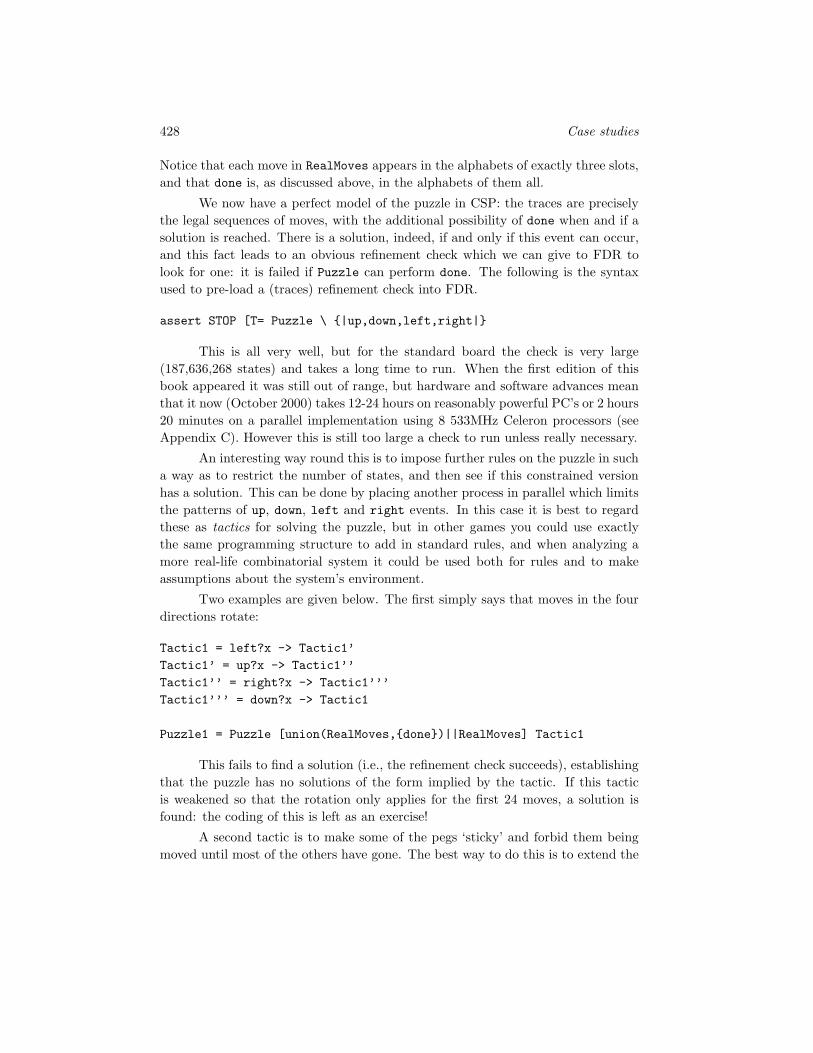
428 Case studies
Notice that each move in RealMoves appears in the alphabets of exactly three slots,and that done is, as discussed above, in the alphabets of them all.
We now have a perfect model of the puzzle in CSP: the traces are preciselythe legal sequences of moves, with the additional possibility of done when and if asolution is reached. There is a solution, indeed, if and only if this event can occur,and this fact leads to an obvious refinement check which we can give to FDR tolook for one: it is failed if Puzzle can perform done. The following is the syntaxused to pre-load a (traces) refinement check into FDR.
assert STOP [T= Puzzle \ |up,down,left,right|
This is all very well, but for the standard board the check is very large(187,636,268 states) and takes a long time to run. When the first edition of thisbook appeared it was still out of range, but hardware and software advances meanthat it now (October 2000) takes 12-24 hours on reasonably powerful PC’s or 2 hours20 minutes on a parallel implementation using 8 533MHz Celeron processors (seeAppendix C). However this is still too large a check to run unless really necessary.
An interesting way round this is to impose further rules on the puzzle in sucha way as to restrict the number of states, and then see if this constrained versionhas a solution. This can be done by placing another process in parallel which limitsthe patterns of up, down, left and right events. In this case it is best to regardthese as tactics for solving the puzzle, but in other games you could use exactlythe same programming structure to add in standard rules, and when analyzing amore real-life combinatorial system it could be used both for rules and to makeassumptions about the system’s environment.
Two examples are given below. The first simply says that moves in the fourdirections rotate:
Tactic1 = left?x -> Tactic1’
Tactic1’ = up?x -> Tactic1’’
Tactic1’’ = right?x -> Tactic1’’’
Tactic1’’’ = down?x -> Tactic1
Puzzle1 = Puzzle [union(RealMoves,done)||RealMoves] Tactic1
This fails to find a solution (i.e., the refinement check succeeds), establishingthat the puzzle has no solutions of the form implied by the tactic. If this tacticis weakened so that the rotation only applies for the first 24 moves, a solution isfound: the coding of this is left as an exercise!
A second tactic is to make some of the pegs ‘sticky’ and forbid them beingmoved until most of the others have gone. The best way to do this is to extend the

15.1 Combinatorial systems: rules and tactics 429
notation used to define the puzzle to include a sticky peg S as well as an ordinaryone P. An arrangement that works well for the standard puzzle is
Board1 = <<X,X,P,P,P,X,X>,
<X,X,P,P,P,X,X>,
<S,S,P,P,P,P,P>,
<P,P,P,E,P,P,P>,
<S,S,P,P,P,P,P>,
<X,X,S,P,S,X,X>,
<X,X,S,P,S,X,X>>
Adopting this extended notation does not change the network produced by theearlier definition of Puzzle, because of the way the process Slot(i,j) was definedabove. It does, however, allow us to define a tactic process to implement ourrestricted search for a solution. The following constants (derived from this newboard) represent the number of pegs that are not to be delayed, and the moveswhich are respectively in the alphabets of any sticky peg and those which are not.
NoDelays = card((i,j) | (i,j) <- BoardCoords, init(i,j) == P)
DelayMoves = diff( Union(Alpha(i,j) | (i,j) <- BoardCoords,
init(i,j)==S),
done)
NoDelayMoves = diff(RealMoves,DelayMoves)
To define the tactic fully we need to know how many moves need to happenbefore a sticky peg can move. Perhaps the cleanest way to do this is to define aconstant NonStickiesLeft which defines how many other pegs are left when thefirst peg marked S can move. This can be used, in conjunction with NoDelays, tocompute the initial parameter for a process that runs in parallel with the system toimplement the tactic.
Tactic2(n) = if n==0 then []x:RealMoves @ x -> Tactic2(0)
else []x:NoDelayMoves @ x -> Tactic2(n-1)
Puzzle2 = Puzzle [|RealMoves|]
Tactic2(NoDelays-NonStickiesLeft)
Provided this allowance is set to be at least 4, the configuration given above(the first one the author tried, and the one described in [108], where the impliedNonStickiesLeft is 5) finds a solution.

430 Case studies
Solving puzzles like this is great fun, and several times we have found solu-tions to other ones which are shorter than the best previously known. (Evidentlyall solutions to solitaire have the same length!) The serious points of this exampleare firstly to show how the constructs of CSP (especially its ability to synchronizean arbitrary number of processes on a given event) allow us to model combinatorialsystems which evolve according to rules, secondly how to add further rules, tacticsor assumptions via parallel composition, and finally to show that model-checkingtools such as FDR really can discover things that are at or beyond the limit of whatthe unassisted human can do.
Most of the exercises in this chapter require FDR or some similar tool.
Exercise 15.1.1 Modify Tactic1 so that it allows any move after 24 rotating onesand find a solution to the puzzle that follows this pattern.
Exercise 15.1.2 A farmer has to ferry a wolf, a goat and a cabbage across a riverusing a boat that is only big enough for him and one of his charges. Unfortunately, withoutthe farmer to control then, the goat would eat the cabbage and the wolf would eat thegoat. Devise a CSP program to find the way the farmer can get all across safely.
Use your program to demonstrate that his task would become impossible if he hadeven one more of any of the cargo items. Would it help him, in that case, to have an islandin the middle of the river?
Exercise 15.1.3 Produce a version of the solitaire script which uses a hexagonal gridlike the two example puzzles shown in the upper part of Figure 15.2, with the pieces nowable to hop in any one of six directions along the lines. Are the puzzles shown soluble, inthe sense that you can end up with a single peg left, in the initially empty slot?
Hint: you might find adapting the script easier if you transform the hexagonal gridto a rectangular one with moves allowed on one set of diagonals, as shown in the bottomof the figure.
15.2 Analysis of a distributed algorithm
In books such as [25] you will find clear but relatively informal presentations of awide variety of distributed algorithms for things like clock synchronisation, trans-action processing, database management and communication. These algorithmsare sometimes presented as a sequence of messages each node has to send andtheir reactions to each, and sometimes as an overall description of the pattern ofcommunication that arise in the system. The purpose of this section is to take aspecific example and to show how, unless one is exceptionally careful, this styleof description can lead to possibly dangerous imprecision. The example we use isof a leadership election algorithm – distributed algorithms frequently depend on

15.2 Analysis of a distributed algorithm 431
Figure 15.2 Hexagonal solitaire (see Exercise 15.1.3).
there being an agreed node who can play some co-ordinating role – called the bullyalgorithm (for reasons that will become apparent).
The following description is paraphrased from p. 306 of [25].
The bully algorithm This is used to allow a group of processors to have anagreed co-ordinator from amongst them, despite the fact that processors may atvarious times fail and revive, The aim is always to have them agree that the co-ordinator is the highest indexed processor that is working. We assume that commu-nication is reliable, but processes can fail at any time (including during the electionprocedure that the algorithm represents).
As with many distributed algorithms, time plays an important role in thisone. Therefore we use the tock-timed dialect of CSP introduced in Chapter 14 tomodel it.
There are three types of message that the algorithm description refers toexplicitly:
channel election:Proc.Proc
channel answer:Proc.Proc

432 Case studies
channel coordinator:Proc.Proc
where Proc=0..N-1, say, and all these represent synchronisations between asender process (the first index) and a receiver.
An election.n.m message is used to announce an election (from n to m);an answer message is sent in response to an election message; and a coordinator
is sent to announce the identity of the new co-ordinator. A process begins anelection “when it notices that the co-ordinator has failed”. This last statementlacks detail about the mechanism by which this noticing of failure is done. We usethe two channels test and ok that are declared here: any process can decide tosend a test message to its co-ordinator, who only sends ok back if it is a properlyworking co-ordinator. This raises the question of what happens if a process tests itsco-ordinator but the latter, though working, does not think is is the co-ordinator!
channel fail, revive:Proc
channel test,ok:Proc.Proc
The first two are communicated when a process fails or revives (allowing us to seewhat the current status of each process is). The last two are used by one processto test another, and to give a positive response to such a test.
To begin an election, a process sends an election message to all those witha higher index. It then awaits an answer message in response. If none arriveswithin time T1, the processor considers itself the co-ordinator (as it thinks all thehigher ones must be dead), and sends a coordinator message to all processes withlower identifiers announcing this fact. Otherwise, the process waits a further limitedperiod (T2), expecting to receive a co-ordinator message as described in the nextparagraph, before beginning another election (if no such message is received).
If a process receives a co-ordinator message, it records the identifier of theco-ordinator contained within it (i.e., the sender of that message) and treats thatprocess as the co-ordinator.
If a process receives an election message, it sends back an answer messageand begins another election, unless it has begun one already.
When a failed process is revived, it begins an election. If it is has the highestlive process identifier, then it will eventually decide that it is the co-ordinator, andannounce this to the other processes. Thus it will become the co-ordinator, eventhough the current co-ordinator is functioning. It is for this reason that the thealgorithm is called the bully algorithm.
For example, consider the case where there are four nodes 1–4, all initiallyworking so that the initial coordinator is node 4.

15.2 Analysis of a distributed algorithm 433
If this node fails, and node 2 tests it, then an election will be started by node2. It sends election messages to 3 (who answers and starts its own election) andto 4, who does not answer. Node 3 will get no answer to its election message to4, and will therefore send everyone a coordinator message. When 4 eventuallyrevives it will realise that it ought to be coordinator (since there is no process withhigher index) and bully all the others into accepting it.
The intention, it would seem, is that except when the co-ordinator has failedand has not been tested since, the nodes either all agree on the correct coordinator(i.e., the live one with highest index) or are in the process of an election which will,in the absence of any further process failures or revivals, produce this result in abounded time. It is that which we will test in this section.
Part 1: Specification
It is, of course, good practice to design your specification before your system. Inthe present case the specification is also rather easier.
Assume all the actions described above, except for fail, revive and test
have been hidden as internal, and do not therefore play a part in our specifications.Assume, furthermore, that there are additional channels
channel tock
channel leader:Proc.Proc
the first showing the passage of time (as in Chapter 14), the second an externalchannel of each process showing who it believes is the current co-ordinator, whichit is prepared to communicate on whenever it is neither failed nor in mid-election.
Basically, what we have to do is to translate the English specification aboveinto CSP. This will require us to interpret some of its parts such as the concept of‘agree’ in CSP terms, and to give concrete interpretation to things like time bounds.
We can capture the intended specification in terms of traces or (more strongly)in terms of failures.
(a) Whenever no process has revived for TS time units, and each fail has beenfollowed by some revive or test event (the two sorts that could set anelection going) at least TS timed units ago, then if any node believes there isa co-ordinator (i.e., communicates leader.m.n) then n is the highest “living”node.There are three basic states to this specification: one in which the conditionis enforced, and two where it is not because either the system is being allowed

434 Case studies
time to settle, or an untested coordinator failure has occurred. All three areparameterised by the set of live processes (ones that have revived since lastfailing).The first case is when the condition is being enforced.
AGREEBY(0,alive) =
alive != & leader?m:alive!max(alive) ->
AGREEBY(0,alive)
[] tock -> AGREEBY(0,alive)
[] fail?k -> (if k==max(alive) then
AGREEBY’(diff(alive,k))
else
AGREEBY(0,alive))
[] revive?k -> AGREEBY(TS,union(alive,k))
[] test?n?k -> AGREEBY(0,alive)
In the second we are waiting n > 0 tocks before enforcing it. Note thatwe allow failures other than the natural leader to reset the timer since theymight well disrupt an in-progress election.
AGREEBY(n,alive) = leader?m:alive?k -> AGREEBY(n,alive)
[] tock -> AGREEBY(n-1,alive)
[] fail?k -> (if k==max(alive) then
AGREEBY’(diff(alive,k))
else
AGREEBY(TS,alive))
[] revive?k -> AGREEBY(TS,union(alive,k))
[] test?m?k -> AGREEBY(n,alive)
Finally, we have the state in which the leader has failed but has not yet beentested. Since either a test or a process revival ought to start an election,either breaks this state.
AGREEBY’(alive) = leader?m:alive?k -> AGREEBY’(alive)
[] tock -> AGREEBY’(alive)
[] fail?k -> AGREEBY’(diff(alive,k))
[] revive?k -> AGREEBY(TS,union(alive,k))
[] test?n?k -> AGREEBY(TS,alive)
The above is, of course, a trace specification. On the assumption that allprocesses start off working properly the natural starting state of this speci-fication is AGREEBY(alive,0).

15.2 Analysis of a distributed algorithm 435
(b) It is, however, easily turned into a failures(/divergences) specification thatsays that under the same conditions all live processes definitely do believe inthe correct leader process. Simply replace the first lines of the second twocases above by themselves nondeterministically composed with STOP, and putthe entire specification in parallel with
CHAOS(|tock,fail,revive,test|)
synchronising on this set of all events that the specification uses other than|leader|.
In addition to these functional specifications, we would obviously like our im-plementation to be deadlock-free and to satisfy the appropriate timing consistencycheck (see page 393).
Part 2: Implementation
Given the freedom with which the nodes potentially run, it seems to be necessary,for the avoidance of deadlock, to make the nodes continually receptive of almost allthe messages that might be directed at them by another node. This even applieswhen the node has failed, since we would expect a dead node to ignore things thatare directed at it rather than prevent them from happening. In other words thisis a case where the handshaken communication of CSP is being used to model asomewhat freer form of interaction.
In programming the nodes you soon realise that, because of the necessity setout in the above paragraph, you have to deal with cases not directly catered forin the English description of the protocol. This is a very common experience intranslating from English to formal specifications. The situations we have in mindhere are ones in which a node is doing what it has to to perform its role in one runof the protocol when it gets interrupted by a message from another run.
For example, if node n receives an election message in the middle of dis-tributing its own coordinator signal, then we might think we ought to abandonthe distribution and get on with the election, after answering the election message.That, however would be a mistake, especially because the coordinator messagemay well have arrived after (and therefore overridden) the election message else-where, including at its origin. If, on the other hand, it ignored an election messagefrom node m in a situation where this was sent subsequent to m having receivedits own coordinator.n (e.g., because m has revived) this could also lead to prob-lems. The right solution to this particular conundrum appears to be that sincenothing has happened to shake n from its belief that it is the rightful co-ordinator,
436 Case studies
the appropriate thing is for it to re-start its coordinator distribution so that theelection sender will definitely receive it again.
We take a minimalist approach to introducing timing into our system. Inparticular we always assume that any response that the protocol calls for from noden without it having to wait for anything else, happens immediately (i.e., before thenext tock). One could perhaps get a slightly more accurate model by introducingsmall delays here, but we would get a more complex model with more states. Andin the end it does not appear to influence the outcome greatly. What the authordid have to do to avoid some oddities and failures of timing consistency was toassume that no process generates more than one test of the co-ordinator in anytime interval, and that at least one tock occurs between any process failing andreviving.
The following definitions set up the number of nodes, and some time delays.We will find later that this particular number of nodes is important.
N=4
Proc = 0..N-1
T1 = 1
T2 = 2
TS = 5
All communications in this algorithm go from high to low or low to high soit is useful to have the following sets defined:
above(n) = k | k <- Proc, k>n
below(n) = k | k <- Proc, k<n
Each process can be in one of a number of states. Let us begin with the onein which it is just starting an election:
BeginElection(n) = SendElections(N-1,n)
which results in it sending successive election messages to the appropriate nodes.Note how it can handle the receipt of any message it might receive, with varyingresults...
SendElections(k,n) = (if k<=n then AwaitAnswers(T1,n)
else election.n.k -> SendElections(k-1,n))
[] election?k’:below(n)!n ->answer.n.k’ ->

15.2 Analysis of a distributed algorithm 437
SendElections(k,n)
[] answer?k:above(n)!n -> AwaitCoordinator(T2,n)
[] ok?k’:above(n)!n -> SendElections(k,n)
[] coordinator?c:above(n)!n -> Running’(n,c)
[] fail.n -> Failed(n)
[] test?m:below(n)!n -> SendElections(k,n)
Below, it is waiting for answers from its election messages, with the time-out making it the coordinator if it has not had one within T1:
AwaitAnswers(t,n) = if t==0 then BecomeCoordinator(n)
else
tock -> AwaitAnswers(t-1,n)
[] answer?k:above(n)!n -> AwaitCoordinator(T2,n)
[] ok?k:above(n)!n -> AwaitAnswers(t,n)
[] election?k:below(n)!n -> answer.n.k ->
AwaitAnswers(t,n)
[] coordinator?c:above(n)!n -> Running’(n,c)
[] fail.n -> Failed(n)
[] test?k:below(n)!n -> AwaitAnswers(t,n)
After it has had an answer message, it sits and waits to be sent a coordinator
message (or any of a number of others), before starting another election if nothingsignificant has happened.
AwaitCoordinator(t,n) = if t==0 then BeginElection(n)
else
tock ->AwaitCoordinator(t-1,n)
[] coordinator?c:above(n)!n -> Running’(n,c)
[] answer?k:above(n)!n -> AwaitCoordinator(t,n)
[] ok?k:above(n)!n -> AwaitCoordinator(t,n)
[] election?k:below(n)!n -> answer.n.k ->
AwaitCoordinator(t,n)
[] fail.n -> Failed(n)
[] test?k:below(n)!n -> AwaitCoordinator(t,n)
The following state represents when it has decided, for want of life above it,that it is the current co-ordinator
BecomeCoordinator(n) = SendCoords(n-1,n)
It distributes a coordinator.n message to all below it. Note that since it is thecoordinator, it sends a positive response to the test message, unlike earlier states

438 Case studies
SendCoords(j,n) = if j<0 then RunAsCoord(n)
else coordinator.n.j -> SendCoords(j-1,n)
[] election?k:below(n)!n -> BecomeCoordinator(n)
[] coordinator?c:above(n)!n -> Running’(n,c)
[] fail.n -> Failed(n)
[] test?k:below(n)!n -> ok.n.k -> SendCoords(j,n)
All the above states represent stages in the election protocol. Obviouslywe also need states in which a process is running, or has failed. When a node isco-ordinator it takes the following state:
RunAsCoord(n) = tock -> RunAsCoord(n)
[] test?k:below(n)!n -> ok.n.k -> RunAsCoord(n)
[] coordinator?k:above(n)!n -> Running’(n,k)
[] election?k:below(n)!n -> answer.n.k ->
BeginElection(n)
[] fail.n -> Failed(n)
[] leader.n.n -> RunAsCoord(n)
and one in which thinks some other node k is coordinator
Running(n,k) = test.n.k -> Testing(n,k)
[] tock -> Running(n,k)
[] coordinator?k:above(n)!n -> Running’(n,k)
[] answer?j:above(n)!n -> Running(n,k)
[] leader.n.k -> Running(n,k)
[] election?k:below(n)!n -> answer.n.k ->
BeginElection(n)
[] test?j:below(n)!n -> Running(n,k)
[] fail.n -> Failed(n)
When it has sent a test message to the node it believes is co-ordinator, it waitsuntil one time unit has passed before deeming the co-ordinator to have failed andbeginning an election. Yet again, it is necessary to allow for anything else thatmight arrive in the meantime.
Testing(n,k) = ok.k.n -> Running’(n,k)
[] tock -> BeginElection(n)
[] answer?j:above(n)!n -> Testing(n,k)
[] coordinator?k:above(n)!n -> Running’(n,k)
[] election?k:below(n)!n -> answer.n.k ->
BeginElection(n)

15.2 Analysis of a distributed algorithm 439
[] fail.n -> Failed(n)
[] test?j:below(n)!n -> Testing(n,k)
[] leader.n.k -> Testing(n,k)
After performing one test successfully, it goes into the following state in which ithas to wait a time unit before performing another one (thereby avoiding a potentialdivergence):
Running’(n,k) = tock -> Running(n,k)
[] coordinator?k:above(n)!n -> Running’(n,k)
[] answer?j:above(n)!n -> Running’(n,k)
[] election?j:below(n)!n -> answer.n.j ->
BeginElection(n)
[] fail.n -> Failed(n)
[] leader.n.k -> Running’(n,k)
[] test?j:below(n)!n -> Running’(n,k)
[] ok?j:above(n)!n -> Running’(n,k)
A failed process just absorbs messages sent to it until
Failed(n) = tock -> Failed’(n)
[] coordinator?k:above(n)!n -> Failed(n)
[] election?k:below(n)!n -> Failed(n)
[] test?k:below(n)!n -> Failed(n)
[] ok?k:above(n)!n -> Failed(n)
[] answer?k:above(n)!n -> Failed(n)
it is revived, which is not until at least one time unit has passed
Failed’(n) = tock -> Failed’(n)
[] coordinator?k:above(n)!n -> Failed’(n)
[] election?k:below(n)!n -> Failed’(n)
[] test?k:below(n)!n -> Failed’(n)
[] ok?k:above(n)!n -> Failed’(n)
[] answer?k:above(n)!n -> Failed’(n)
[] fail.n -> Failed(n)
[] revive.n -> (if n==N-1 then BecomeCoordinator(n)
else BeginElection(n))
Note that if the highest-index process revives it has no need to carry out an electionto know it should be co-ordinator.

440 Case studies
We can then give each process its obvious alphabet and run them in parallelas a network.
Alpha(n) = union(|tock, fail.n, revive.n, election.n,
coordinator.n, test.n,
answer.n, leader.n, ok.n| ,
election.k.n, coordinator.k.n,
test.k.n, answer.k.n, ok.k.n| k <- Proc)
Node(n) = if n==N-1 then RunAsCoord(n) else Running(n,N-1)
Network = || n:Proc @ [Alpha(n)] Node(n)
The first thing to try with any timed example is a timing consistency check along thelines set out on page 393. The following events are all deemed ‘delayable’ becausewe do not want to have to rely on them happening urgently for time to pass (theinclusion of test here serves the purpose of showing that the individual nodes canbe ‘lazy’ about instigating tests of they want to be, though we will later be forcedto re-think this in some circumstances).
Delayable = |fail, revive, leader, test|
Urgent = diff(Events,union(tock,Delayable))
The following give us two nearly equivalent ways of testing it, the second beingstronger because it proves that hiding the urgent events can’t introduce divergence,which would break various assumptions of the abstraction method.
assert TOCKS [F= (Network [|Delayable|]
CHAOS(Delayable))\diff(Events,tock)
assert TOCKS ||| CHAOS(Delayable) [FD= Network \ Urgent
TOCKS = tock -> TOCKS
15.2.1 Analysis
With the values of the parameters given, the timing consistency checks succeed,meaning that our model makes sense as a timed system. Fascinatingly, however,the others fail, even though we have done our best to implement the algorithm fromthe literature. A typical error trace follows (though it is far from unique):
fail.2, fail.3, test.1.3, tock,

15.2 Analysis of a distributed algorithm 441
election.1.3, election.1.2,
revive.2, revive.3, coordinator.3.2,
fail.3, test.0.3, tock,
coordinator.1.0, tock,
tock, tock, tock, leader.2.3
This can be interpreted as follows:
1. Nodes 2 and 3 fail.
2. Node 1 tests node 3; when it gets no response an election is started.
3. Both 2 and 3 revive shortly after they miss (through being failed) the electionmessages they get from 1.
4. 3 manages to tell 2 it is the coordinator before failing again.
5. 0 begins a test of 3.
6. By this time, 1 decides that since it has not had any response to the electionit started, that it is the rightful co-ordinator. It therefore tells 0, whichpre-empts the test the latter is doing.
7. The specification then gives the system time to settle (the tock events to-wards the end of the trace), though nothing of significance actually happensin this time.
8. We are left in a state where 0 and 1 believe 1 is the co-ordinator, and 2believes that 3 is (though 3 has failed). Actually, of course, 2 ought to be.
It is the way various elections get mixed up, and the way in which processes canfail in the middle of broadcasting a message to the others, that causes the problem.These two themes are common to about every error the author has examined tocome out of FDR. Indeed, if process failure is prevented during the SendCoords
phase of broadcasting coordinator messages, all the specifications succeed.
The impossibility of this sort of failure might or might not be regarded asa reasonable assumption, though it would appear a dangerous one if the messagesreally do get sent out one after another. If not, the fact that the protocol appearsto work if we do assume it provides a clue as to how we might correct the program.We need to guard against only some of the nodes that ought to be informed aboutn’s co-ordinator status getting this message. The dangerous scenario following thisappears to be that one of the nodes who has not heard the coordinator.n messagetests who it thinks is the coordinator, which is sufficient for the specification to thinkthat the network ought to settle to a correct state. One way to avoid this is to ensurethat each node m that gets a coordinator.n tests n long enough after so that if
442 Case studies
this succeeds then it knows the broadcast has not been interrupted, for if the testfails then a new election will be started, and the inconsistent state will be clearedup. It is sensible to extend the minimum possible time between node failure andrevival, to make sure that n as discussed above has not done these things betweenm getting coordinator.n and completing the test of n. (If such an assumption isnot realistic, nodes could simply be programmed to wait an appropriate time afterrevival before doing anything.)
It is straightforward to adapt our program to encompass these extra testsand delay assumption. One slight complication arises from the timing model: in thefirst model it was helpful to think of the test events as delayable, since we did notwant to rely on them happening simply to allow time to progress. We would stilllike to take this view of the tests that arise ‘optionally’, but it does not fit with thecompulsory tests that happen after being sent a coordinator event. To solve thiswe make test.n events urgent, and guard each optional test with a new delayableevent dotest.n.
Thus the following state can perform dotest, which takes it
Running(n,k) = dotest.n -> Testing1(n,k)
[] tock -> Running(n,k)
[] coordinator?k:above(n)!n -> Running’’(n,k)
[] answer?j:above(n)!n -> Running(n,k)
[] leader.n.k -> Running(n,k)
[] election?k:below(n)!n -> answer.n.k ->
BeginElection(n)
[] test?j:below(n)!n -> Running(n,k)
[] fail.n -> Failed(n,TR)
to the Testing1 state, which actually starts the test proper.
Testing1(n,k) = test.n.k -> Testing2(n,k)
[] answer?j:above(n)!n -> Testing1(n,k)
[] coordinator?k:above(n)!n -> Running’’(n,k)
[] election?k:below(n)!n -> answer.n.k ->
BeginElection(n)
[] fail.n -> Failed(n,TR)
[] test?j:below(n)!n -> Testing1(n,k)
[] leader.n.k -> Testing1(n,k)
Testing2(n,k) = ok.k.n -> Running’(n,k)
[] tock -> BeginElection(n)
[] answer?j:above(n)!n -> Testing2(n,k)

15.2 Analysis of a distributed algorithm 443
[] coordinator?k:above(n)!n -> Running’’(n,k)
[] election?k:below(n)!n -> answer.n.k ->
BeginElection(n)
[] fail.n -> Failed(n,TR)
[] test?j:below(n)!n -> Testing2(n,k)
[] leader.n.k -> Testing2(n,k)
Here, Running’(n,k) a state like Running(n,k) except that it will not instigatea further test until after a tock. Running’’(n,k) is a state that moves to stateTesting1(n,k) after one tock, thereby testing the co-ordinator one time unit aftercoordinator.k is received.
With this amendment, the protocol meets its specification for all the cases(with reasonable timing parameters) that we have tried.
15.2.2 Conclusions
There are a number of observations we might make about this case study. Duringthe process of creating the program for the bully algorithm set out above, therewere far more problems encountered than is obvious from how we have describedit. Specifically, a number of iterations of the program failed deadlock or timingconsistency checks, usually because the author had not allowed for various sorts ofmessages arriving at nodes who (one might have thought) were not really expectingthem. The fact that these messages had to be handled, and the decisions abouthow to handle them, impressed on him that the English description of the protocolleft more unanswered than one might think on first reading it.
Having ironed out these problems, we were left with an apparently workingmodel (the uncorrected one presented above). Indeed, for three nodes all the spec-ifications of it succeed, though as we have seen four is sufficient to find problems.It doesn’t seem likely that many humans would find the ways in four nodes have tointeract in order to find the subtle problems FDR discovered. Indeed, the authorhad taught the bully algorithm in tutorials for several years without spotting them.It was only the feeling that there were stones left unturned in the arguments weconstructed annually as to why the algorithm worked that led to this FDR analysis.
It is hard to say that the problem we encountered with inconsistent statesfor four or more nodes represents a definite error in the algorithm itself. Whatit does show is that a highly plausible implementation of the algorithm can failwhat looks like an equally plausible formalisation of its specification. The authoronce used this example as an end-of-course assessment for Masters students, givingthem the English description and a few hints on how to create the necessary CSPspecifications and implementations. A majority of the students found essentially

444 Case studies
the same problem, and in at least one case a different problem that occurs whenthe order in which broadcast messages are sent out is changed. This might be takenas evidence that, at least for this algorithm, simply implementing what you finddescribed in English in a book is far from being a guarantee of correctness.
The fact that the original implementation worked for three but not fournodes is both interesting and worrying. The only Masters student who made aserious attempt at correcting the problem uncovered at four nodes came up with aversion that worked for four but not five nodes – amazingly enough repeating whathad happened to the author on an earlier attempt at correcting the system. Theseexperiences are likely to leave anyone worried that the corrected version might workup to some limit (say 10) and after that fails in a system of such size that FDRcannot handle it.
One method for addressing this scaling problem, but unfortunately not onethat can be used (at least, straightforwardly) to address the current example, canbe found in the next section. The best option for a general proof would appearto be mathematical induction. This would probably take the form of showing thatthe uppermost k nodes of our implementation meet some condition that implies thespecifications when all n nodes are present, and which is closed under the inductivestep of attaching a further node at the bottom. The basic properties one wouldrequire are fairly obvious, namely that within appropriate time limits of either anelection message being sent from below (when one of the k is alive) or a processfrom the k reviving, an appropriate coordinator broadcast occurs. As with theoriginal protocol description, this broad brush specification ignores lots of nuances,and it seems certain that any working inductive hypothesis would have to deal withmany of these. This is not something we have yet done.
This example thus displays both the strengths of the automated approach –since it found errors a human was unlikely to discover and allowed us to correctthese at least to the bounds of FDR’s capabilities to handle the resulting system –and one of its main weaknesses.
Exercise 15.2.1 Observing that it is node n-1 who is the first recipient of any batchof coordinator messages from node n, it is plausible to suggest that only this node needsto instigate the test of node n that was introduced in the correction. Is this correct? (Youshould first attempt to solve this problem without using FDR on a modified file, but canof course use this method should you not be sure of the answer you then get.)
Exercise 15.2.2 Are the answer.n.m messages a necessary part of the protocol? If so,why, and if not can you suggest any pragmatic arguments as to why they are neverthelessthere?
Exercise 15.2.3 Consider the following modification to the algorithm. There arenow two sorts of election message. Elections caused by someone noticing co-ordinator

15.3 Distributed data and data-independence 445
failure use one sort, and follow exactly the same path as before. Elections caused bya node reviving use an election’ channel, with the property that when a node who isrunning normally receives it, it simply tells the sender who the coordinator is via a channelcoordinator’.n.m.c (n telling m that the co-ordinator is c). If a reviving node has notbeen sent such a message or an answer (sent by nodes receiving election’ when they arein the process of an election themselves) within a reasonable time, it deems itself to be theco-ordinator and broadcasts this fact as before.
Does this work (a) when the uncorrected program is modified accordingly, and ifnot, (b) the corrected one is modified so that only coordinator as opposed to coordinator’messages force a test, and if not (c) the corrected one is modified so that both sorts forcea test? What advantages and disadvantages do you see for this new approach?
15.3 Distributed data and data-independence
Many of the applications CSP is best suited to are systems that handle data itemswithout altering them. Rather they manage data values, and input and outputthem – hopefully at appropriate times on the desired channels. We have seen manyexamples in buffers and communication protocols, stacks and bags. Some of themost striking examples are systems that store multiple copies of data (either forsecurity against failure or speed of access) but seek to maintain the appearance ofa single copy which can be accessed for reading and writing.
In this section we see two of these: one where copies of a store are heldat every node on a ring, and a model of a cache not unlike those used on mostmicroprocessors. One of our main objectives is to explain and illustrate the theoryof data-independence, whereby it is often possible to prove facts about processes ofthe type described in the previous paragraph for any data type by showing theyhold for a particular finite data type.
15.3.1 A ring database
Imagine that you have a ring of processes, each holding a copy of a selection ofregisters, and that you want each node to be able to update any of these. Anupdate is first executed locally, and then transmitted around the other nodes inturn until it arrives back home. See Figure 15.3. If two nodes at opposite sides(A and D , say) of the ring choose to update the same register at very nearly thesame time, it is evident that the resulting updates will be seen in different ordersif they both simply pass all the way round the ring. This, in turn, might lead to asituation where even after all updates have completed their journeys, nodes B andF disagree on the value of the register.
Unless some sort of locking mechanism is employed – inevitably expensivein time and effort – it is certain that we must put up with there being instants

446 Case studies
Z
WXY
Z
WXY
Z
WXY
Z
WXY
Z
WXY
Z
WXY
A
B
C
D
F
E
Figure 15.3 The ring database.
where simultaneous reads to the same register will yield different results. What wecannot tolerate is any inconsistency which persists, like the one described above,even when the system is quiescent. The author proposed several related algorithmsin [106]3 which guarantee at least this degree of consistency under various scenarios:the simplest one is described below.
Let the nodes on the ring be Ni for 0 ≤ i < M , with indexes increasing inthe direction messages pass round. The user of any node may read or write anyof a set of registers locally. When a local write has occurred, Ni will generate anupdate that is entered into the ring to carry the new value round the other nodes.
3In that paper they are proved mathematically. The mathematical arguments have the advan-tage that they apply to any size of ring, and yield rather more detail about the pattern of valuesvisible than we do here: provided the priorities are restructured to follow a logical time regime, aform of sequential consistency can be proved. They have the disadvantage of being very far fromtrivial, and also do not address questions such as deadlock and livelock freedom as we will here.

15.3 Distributed data and data-independence 447
If otherwise uninterrupted, an update passes round until it arrives back at the nodethat generated it; updates thus carry the identity of their origins with them, andeach node keeps a list Ei of the updates it has generated that are expected back.
In order to resolve the inconsistencies that can arise due to simultaneouslyexisting updates to the same register, the nodes are all assigned unique priorities:let pi be the priority of Ni . These affect what happens when an update u originatedby Ni arrives at Nj :
• If i = j then u is removed from the head of Ej provided it is there. Its absenceis an error: we can deal with it any way we please. In the implementationbelow we do not notice it belongs to the node if Ej is empty, and so it justgets executed and passed round. Other options would be to STOP locally ortransmit some error event.
• If i = j and there is no clashing update (i.e., an update of the same location)in Ej , u is executed locally and passed on round the ring.
• If pi < pj , and Ej contains any updates that clash with it, then u is stopped:it is neither passed on round the ring nor executed locally.
• If pi > pj , and Ej contains any updates that clash with it, then u is executedlocally and passed on round the ring, and the clashing updates are cancelled(removed from Ej ).
In studying this algorithm it is plainly sufficient to consider only a singleregister (i.e., each node has a copy of this register), since, while updates to thesame location interfere with each other in a complex way, ones to different locationsdo not. Thus, in building our implementation we will restrict ourselves to thatcase. This has the twin advantages of somewhat simplifying the programming andreducing the size of the state space, though it would not be difficult to adapt thedefinitions to deal with any number of registers.
It is clearly desirable that the system we build is free of deadlock and livelockas well as satisfying consistency results. There would be no hope of achievingthis if the underlying mechanism that transports updates round the ring coulddeadlock or livelock. We therefore base this aspect of our system on sound principles,namely Deadlock Rule 8 (see page 363) in a way similar to the message-passing ringdescribed with the rule. Specifically we give each node the capacity to hold two(travelling, as opposed to expected-back) updates, but only allow it to become fulldue to an input from the ring.
Our later specifications will be predicated on what the system looks like whenit is quiescent (no updates circulating and none expected). This is the role of theevent quiet: each node can communicate it when it is locally quiescent; we force

448 Case studies
them all to synchronize on it so that the event can happen when, and only when, thewhole system truly is quiescent. This event is not one that would be part of a realimplementation; it is simply something we will need for the purpose of specificationand verification. It actually has a lot in common with the event done from theprevious section, since they are both synchronized over all processes to identify aparticular global state.
The processes defined below do not actually hold the local copy of the register:we will later combine each of them in parallel with a process that does. What theydo is handle updates according to the above algorithm, assuming that any that areinput have already been executed on local data and that any output are immediatelyapplied (at the point of output).
Below, N0(i,E,T) represents the node Ni which presently holds no travellingupdates, and which is expecting the list E of updates back from the ring. Theparameter T is the type which is being stored in the register: the reasons for makingthis explicit will become apparent later. We impose a limit on the length of E sincethis is necessary to keep the process finite state.
N0(i,E,T) = (#E<limit) & in.i?x:T -> N1(i,E^<x>,i,x,T)
[] #E==0 & quiet -> N0(i,E,T)
[] ring.i?j?x:T -> (if #E==0
then (out.i.j!x -> N1(i,E,j,x,T))
else (if i==j
then N0(i,tail(E),T)
else (if priority(i)<priority(j)
then (out.i.j!x -> N1(i,<>,j,x,T))
else N0(i,E,T) )))
The connections of the channels when these are put in parallel are shown in Figure15.4. Since there is only one register, there is no need to name it when passingupdates round the ring. The communication ring.i.j.x means the passing to Ni
round the ring of an update to the register originated by Nj of value x . In theabove state our node can (subject to the limit on E) accept inputs either from itsenvironment or the ring. When it already holds an update j.x which it is readyto output on the ring, then because of the requirements of Deadlock Rule 8, it willonly accept a ring input, but otherwise it behaves similarly.

15.3 Distributed data and data-independence 449
N1
N0
N5
N4
N3
N2
ring.0
ring
.5
ring.1
ring.4 ring.3
ring.2
out.0in.0
in.5
out.5
out.4
out.3
out.2
out.1
in.1
in.2
in.3
in.4
Figure 15.4 Communications in the implementation.
N1(i,E,j,x,T) = ring.((i+1)%M)!j!x -> N0(i,E,T)
[] ring.i?k?y:T ->
(if #E==0
then (out.i.k!y -> ring.((i+1)%M)!j!x -> N1(i,E,k,y,T))
else (if k==i
then N1(i,tail(E),j,x,T)
else (if priority(i)<priority(k)
then (out.i.k!y -> ring.((i+1)%M)!j!x ->
N1(i,<>,k,y,T) )
else N1(i,E,j,x,T) )))
Since the capacity of these nodes is 2, whenever they are full they insist on out-putting on the ring before accepting any more inputs. The ring can then be assem-bled as follows.
Alpha(i) = |in.i, out.i, ring.i, ring.(i+1)%M, quiet|
RING(T) = (|| i:NodeNames @ [Alpha(i)] N0(i,<>,T))\|ring|

450 Case studies
It is natural to split the desired properties of this system into safety (traces)and liveness (failures/divergences) specifications. For this basic ring without regis-ters, one can identify three different liveness checks.
The first and most obvious is deadlock freedom, established, for example, viathe check4
DF [F= RING(T) (1)
It is not too hard to see that the ring as constituted is divergence-free, becauseeach time a hidden action occurs (i.e., a communication on ring), this is precededby either the input (in) or an output (out) of the relevant update. It is, however,interesting to ask whether the process RING(T)\|out| can diverge.
CHAOS(Events) [FD= RING(T)\|out| (2)
Such a divergence would correspond to one or more updates circulating endlesslywithout the need for further input; this is plainly not meant to happen but couldif an update ever arrived back home to find the relevant Ej empty (i.e., it was notexpected).
Assuming that both deadlock freedom and this extended form of livelockfreedom have been proved as they can be (for given implementations) with FDR,the final liveness check we use is to establish that, on the assumption that nodesare never prevented by the environment from outputting updates, they inevitablystabilize in the quiescent state. In other words, left to its own devices, the ringwill eventually come back to the state where no updates are active and none isexpected back. We need to show that, eagerly abstracting the output events andlazily abstracting the input events, the ring failures refines the process
QS = quiet -> QS
The abstracted process can be represented and checked as follows:
QS [F= MixedAbstraction(|in|,|out|,RING(T)) (3)
where the mixed abstraction operator is defined
MixedAbstraction(D,E,P) = (P[|D|]CHAOS(D)) \(union(D,E))
See Section 12.2 for more details of this style of specification using abstraction. Thisparticular check has much in common with the style of timing consistency checkdescribed on page 415. A more direct and equivalent check is to show that
4The checks in this section are numbered so we can refer to them later.

15.3 Distributed data and data-independence 451
CHAOS(|in|) ||| QS
is failures or, equivalently, failures/divergences, refined by RING(T)\|out|.
Now that we know that our system always returns to the quiescent state, anatural way of formulating the basic safety specification (namely, consistency) is toassert that whenever it is quiescent all the copies of the register are equal. One cando this directly on the process RING(T) described above by carefully monitoringthe pattern of updates that occur in each node within the specification. This isdone as an alternative in the example file which illustrates this section, but herewe concentrate on the more obvious method, which is to add the actual registersinto the network. The following definition adds a new channel read, but identifieswrites to the register at node i with the communications in.i.x. There is nothingessential about this approach and writes could also take place on a separate channelprovided the register process carried a flag which indicates whether an update needsto be sent to the ring. (It would be set just when a local write had occurred morerecently than the last communication on in.i or out.i.)
VAR(i,x,T) = (out.i?j?v:T -> VAR(i,v,T))
[] (in.i?v:T -> VAR(i,v,T))
[] read.i!x -> VAR(i,x,T)
VARS(x0,T) = ||| i:NodeNames @ VAR(i,x0,T)
DDB(x0,T) = (RING(T) [||in,out||] VARS(x0,T))\|out|
Here x0 (ranging over the type T) represents the initial value of the register.
The appropriate trace specification is then simply that whenever a quiet hasoccurred more recently than a write (i.e., in this case an in event), two reads willgive the same answer. This can be established by showing that
SS [T= |˜| x0:T @ DDB(x0,T) (4)
where the specification process SS is defined
SS = quiet -> Q0
[] read?j?x -> SS
[] in?j?u -> SS
Q0 = read?j?x -> Q1(x)
[] quiet -> Q0
[] in?j?u -> SS

452 Case studies
Q1(x) = read?k!x -> Q1(x)
[] quiet -> Q1(x)
[] in?j?u -> SS
Note that Q1(x) only permits one value to be read (any other leading to a failureof refinement) whereas the other two states permit any. This is because Q1(x)
represents the case where at least one read (giving value x) has occurred since aquiet event and before any further input on in.
15.3.2 Data-independence
Processes often have one or more parameters, namely quantities or objects that canvary giving different instances of the system. Only the very simplest CSP processesare usually defined without using parameterization at all. Parameters are typicallyused to help capture the states of individual processes or to create a number ofsimilar components to include in a network (e.g., PHILi), but often a completenetwork will still depend on one or more parameters (such as the total number ofphilosophers). The parameters of the distributed database in the previous sectionare:
1. The data type T of stored values.
2. The number of nodes.
3. The limit on the sizes of expected-back queues.
4. The ordering on nodes used to determine priority.
In addition, one could address the question of whether it was buffer tolerant (asdiscussed in Section 5.2) and regard the sizes of the buffers as parameters.
What we would really like to do is prove all the results about liveness andconsistency of the database independently of these parameters. However, tools likeFDR generally only address one specific instance at a time and are usually only cap-able of handling ones with relatively small values for variable-sized parameters suchas the first three above. The general Parameterized Verification Problem (PVP), ofwhether a system satisfies a correctness condition for all parameter values, is cer-tainly formally undecidable [4] (it being easy to reduce other undecidable problemssuch as the halting problem to it), but the subject of looking for specific classesof problems where it might be made tractable is an active area of research (over amuch wider range of theories than simply CSP) and will probably remain one formany years to come.

15.3 Distributed data and data-independence 453
At the time of writing the most progress, by far, has been made with para-meters of the first sort described above, namely data types, and this section isdevoted to presenting the most accessible and useful results about these.
A data type T used in a program P can fairly be said to be a parameter ifP treats it data-independently : it can input and output values of type T along itschannels, store them for later use, but never perform any ‘interesting’ computationson them that constrain what T might be. (For example, if members of T were addedto each other, they would have to be numbers, . . . ) With one or two exceptions,the criteria for deciding whether a type is data-independent are identical to thosefor deciding whether it is a free polymorphic type variable in the sense of languagessuch as ML. Precise criteria for this, which are readily automatable, can be foundin [65], but the following are the main principles:
(i) Concrete values from T (such as 0, true, etc.) may not appear in the programtext of P , though abstract constant symbols can appear.
(ii) You may use basic polymorphic operations on T such as tupling, list forma-tion and suitable operations for extracting members of structures built out ofT in these ways. Intuitively these can be thought of as operations which passmembers of T around without looking inside them at all. No other functionswhich involve T either in the types of their arguments or result may be used.
(iii) No predicate (in a conditional) used in the program can depend on valuesfrom T . The only exception to this rule is that we allow equality (andinequality) tests between members of T . We do not, however, allow ordercomparisons such as ≤ and >.
(iv) Operations such as card(S) (the size of a set) may not be applied to any setinvolving set T . (This would give a way of extracting information from Tthat could be used to influence how P behaved.)
(v) No replicated constructs except nondeterministic choice (|~| x:S @ Q(x))can appear in the process if their indexing set depends in any way on T .Thus, parallel and external choice constructs indexed over T are banned,though the effect of the latter can, in practical circumstances, almost alwaysbe recovered using input (c...?x:S...), which is allowed.
Typical data-independent processes are COPY (in the type communicated)and all the processes in the section on the distributed database (in the parametertype T).
A data-independent program over type T makes sense whatever non-emptyset is substituted for T . If Spec and Impl are two of them, then it makes sense toask questions such as

454 Case studies
• Spec T Impl?
• Spec F Impl?
• Spec FD Impl?
• is Impl deterministic?
for any specific T . Anybody performing many checks of this sort quickly comes tothe conclusion that there must be a strong relationship between the answers to thesequestions for different sizes of T (it being relatively easy to see that the answer forany pair of T ’s of the same size must be the same). Fortunately this intuition istrue and in almost all cases there is a threshold: an integer N such that the answerto one of the above questions for a type of size M ≥ N is independent of M . Inother words, one can prove or refute a result for all sufficiently large5 T via onecheck on FDR.
It is obviously of great practical importance to determine when these thresh-olds exist, and to find as small a threshold value as possible for each question we arepresented with. There is a recently developed theory, too complex to present here,which allows the computation of thresholds by an extension of the theory of logicalrelations (or parametricity) to processes, by augmenting the operational semanticsand CSP normalization to encompass terms with free variables as symbols for mem-bers of the independent type, and by using techniques for exploiting symmetry instate spaces. For details of this theory, see Section 15.5 and [68, 64]. Referencesto related work can be found in these papers and in Section 15.5. What we canpresent here are the main conclusions.
There are four main factors which influence the size (and in some cases theexistence) of a threshold for a given refinement check. These are
• the extent to which the specification constrains which members of T arecommunicated,
• the kinds of equality checks between members of T that are present in thespecification and implementation,
• the subtlety of any nondeterminism in the specification, and
• the extent to which any values of type T which the specification uses arerecorded in its traces (rather than only having some ‘behind the scenes’effect)
5Where there is such a threshold N the answer for sufficiently large finite T also applies to allinfinite T .

15.3 Distributed data and data-independence 455
Lazic has proved a wide variety of results for calculating thresholds for re-finement and determinism checks, falling into four main categories. The followingsections present the central ideas and results from each. Often the result presentedcan be improved (e.g., by weakening its assumptions or strengthening its conclu-sions) if, for example, we are interested only in traces refinement: the interestedreader should consult [65, 68, 64].
When | T |= 1 is enough
One frequently wants to prove specifications of data-independent processes that donot say anything of significance about how they are permitted to handle membersof T . Examples are deadlock and divergence freedom and any trace specificationthat is always happy to allow any member of T in an event when it allows one.It turns out that in many cases it is sufficient to prove such specifications for thesimplest possible T : a one-element type. In other words, the threshold is just 1.
Equality tests over T are banned altogether from both the specification andimplementation6:
NoEqT A data-independent process P satisfies this when it contains no test ofequality between members of T .
All the processes of the distributed database example satisfy NoEqT, as do COPYand all the other buffer and similar examples we have seen.
NoEqT effectively rejects the liberal side of condition (iii) in the definitionof data-independence. To ensure that the specification basically ignores T we assertthat the only way a member of T can occur in a communication of the specificationprocess Spec is via a nondeterministic selection of the form a$x:T -> P which isintroduced as an abbreviation for
|~| x:T @ a.x -> P
(For the purpose of trace specification, this is equivalent to a?x:T -> P.) In otherwords, Spec can never specify which member of T is communicated or that any
6It should be pointed out that there are ways of introducing ‘hidden equality tests’ into CSPprograms via some operations and predicates on sets and sequences, and via communication. Thecommunication effect appears when we synchronize on two output events: c!x -> P [||c||]c!y -> Q contains an implicit equality check between x and y and therefore violates NoEqT.These problems do not appear in the great majority of practical programs and can be avoidedprovided the only set constructs used involving T are unioning of straightforward channel alphabets(for synchronization and hiding), and each synchronization over channels of type T only has oneoutput. If you are in doubt about the legitimacy of some construct you should consult one of[65, 64].

456 Case studies
more than one arbitrary member of T is offered. We will only use the $ form onthe specification side of refinement, since it will always be permissible to re-writeones in the implementation using the more general |~| as above.
The characteristic processes DF of deadlock freedom and ChaosΣ of diver-gence freedom satisfy these criteria, as do processes like
ALT = a$x:T -> b$x:T -> ALT
This particular example just says that communications over a and b alternate with-out placing any constraint on which members of T appear.
We can now state the first of a number of results establishing exact criteriafor data-independent reasoning.
Theorem 15.3.1 Suppose we have processes Spec(T ) and Impl(T ), each data-independent with respect to the type parameter T and additionally satisfying con-dition NoEqT. Suppose further that Spec is restricted to nondeterministic selec-tions over T as described above. Then, with representing any of T ,F ,FDthe result of the refinement check
Spec(T ) Impl(T )
is independent of which non-empty T is used. In particular, the answer for all T isanswered by the check when T = 0 is a one-element type.
What this result says, in essence, is that if we have a program whose control-flow does not depend on which members of T it holds, and a specification whichignores how it handles members of T relative to each other, then we can collapseT to a single value without affecting the result of a refinement check. Obviouslythis will usually give a significant advantage in state space size. It applies to checks(1–3) from the distributed database example.
In fact, essentially the same result holds when Impl is, in addition, allowedto use arbitrary functions whose result is of type T . These processes, which we canterm weakly data-independent, can thus calculate values in T in non-trivial ways,but still cannot let T affect their control-flow. See [67, 68, 65, 64] for details.
When | T |= 2 is enough
If we build a system which is data-independent in some type T then it is likelythat we will want to prove things about how it handles members of T as well asspecifications that ignore T like those dealt with above. It turns out that, providedwe make the same assumptions about the implementation as in the previous section(i.e., it is data-independent and satisfies NoEqT), and follow a set of conditions

15.3 Distributed data and data-independence 457
on the specification designed to remove ambiguity about what state it is in after agiven trace, then we can assume that T has just two elements. In other words, thethreshold is then 2.
The following condition states, in essence, that the specification is alreadynearly in the normal form for CSP used in the algebraic semantics (Section 11.4)and in refinement checking (Appendix C).
Norm A process Spec meets this condition if
(i) its definition contains no hiding or renaming;
(ii) the only parallel operators allowed are alphabetized parallel P[X||Y]Q andits replicated version;
(iii) other than the nondeterministic selection construct7 a$x:S -> P describedabove, no indexed nondeterministic choice is used whose indexing set de-pends on T ;
(iv) all internal and external choice constructs (Q |~| R, Q [] R, indexed ver-sions of these, and [> (the ‘time-out’ operator)) have the initial events ofeach argument disjoint (i.e., once one event has occurred we must knowwhich branch was chosen) and
(v) any uses of the operators ; and /\ ( , the interrupt operator) conform tosome technical conditions given in [65] which essentially ensure that (iv) isnot broken implicitly.
The main role of this condition is to avoid the introduction of any nondeterminismexcept when its effects are immediately apparent. Almost all natural specificationprocesses one ever builds satisfy this condition, or could easily be transformed toones that do, since in order for us to know what a specification says it should beclear what state it is in after a given trace. In other words, Norm can be regardedalmost as a well-formedness condition on specifications in a wider sense.8
Theorem 15.3.2 Suppose Spec and Impl are data-independent processes, bothsatisfy NoEqT and Spec satisfies Norm. Let be any of T ,F ,FD.
7It is legitimate to use complex prefixes such as c$x$y?z, but for technical reasons (see [68, 64])you may not mix (either here or anywhere else the nondeterministic selection construct is used inthe study of data-independence) nondeterministic selections over T with inputs over types otherthan T .
8The only major class of specifications we have seen that do not fall within this categoryare the fault-tolerance specifications such as NoFaults on page 318. These, being derived fromimplementations, may very well contain hiding, etc.

458 Case studies
• If Spec(2) Impl(2) holds (i.e., for T of size 2) then Spec(m) Impl(m)holds for all finite and infinite m ≥ 1.
• If the refinement Spec(2) Impl(2) fails then Spec(m) Impl(m) fails forall finite and infinite m ≥ 2.
The difference between this result and the previous one is that here there isnothing to prevent the specification restricting which of the values of T it knowsabout is communicated after a given trace. Also, in the case of failures and fail-ures/divergences specifications, it can specify much more about which refusal setsinvolving members of T are acceptable. Thus, for example, any of the processesBUFFN
〈〉 and WBUFFN〈〉 from Section 5.1 would be acceptable for Spec in this result
but not for Theorem 15.3.1.
Intuitively, this result says that if we have both an implementation and aspecification which pass members of T around without letting them determine thecontrol-flow, then in order to check whether a refinement holds it is sufficient tolook at T of size 2. What you have to check in these cases is that each value inputinto an implementation is output in just the right places. In [67, 68, 65, 64] itis shown that in many cases you can restrict the state space of the check further:although it still requires a data type of size 2, one can assume that all but one of thevalues input into the implementation are equal. These references also contain (i)significant strengthenings of Theorem 15.3.2 which depend on definitions we havenot had space for here, and (ii) discussion of the extent to which specifications thatdo not satisfy the condition Norm can be transformed into ones that do via anequivalent of the normalization procedures described in Section 11.4 and AppendixC.
The consistency check (4) of the distributed database, as well as most of theearlier correctness conditions of communications protocols and similar processes,come directly within the scope of the above theorem, however. Thus all the checksin the previous section have, as far as the type parameter T is concerned, a thresholdof 1 or 2.
There is an important generalisation to this case that we ought to mentionhere, since it will be important in the section on cryptographic protocols. This isthat many of the results in this subsection continue to hold if we relax our insistencethat there are no equality tests and replace it with conditions that permit equalitytests but only allow progress when equality is true. In other words, we allow thetests in contexts like
if e1 == e2 then P else STOP
where e1 and e2 are expressions of the data-independent type. The precise form of

15.3 Distributed data and data-independence 459
both the booleans in these conditional and the process P depends on which form ofthe condition we are using.
A process description is said to satisfy PosConjEqT when it contains noequality tests (explicit or implicit) which can result in some behaviour on inequalitythat is not possible on equality (other than on tests for equality with constantsymbols). For a formal definition see [64].
The general case
The definition of data-independence quoted at the start of this section allowed forequality tests between members of T . Thus the process
RemDups = left?x -> right!x -> RemDups’(x)
RemDups’(x) = left?y -> if x==y then RemDups’(x)
else right!y -> RemDups’(y)
which removes adjacent duplicates from a stream of values is data-independent eventhough its control-flow depends on the values of T it uses. Evidently, however, thisdoes not satisfy the condition NoEqT, and so neither of the earlier results applies toit. In cases like this it is still, under appropriate conditions, usually possible to findthresholds, but they vary with the complexity of the processes under consideration.For example, a process which inputs N values and then communicates a only ifthey are all different plainly needs a threshold of at least N in order to show thatit can sometimes communicate a.
Lazic has shown how to compute thresholds in terms of the following quanti-ties. Bear in mind that we are going to assume that the specification Spec satisfiesNorm whereas no such assumption will be made of Impl.
W Impl is the maximum number of values of type T that the implementation Impl
ever has to store for future use. This number can be computed by go-ing through the operational semantics of the process in such a way thatmembers of T are treated as ‘symbolic’ identifiers and counting how manyof them are required in any state. For the RemDups example above, thisnumber is 1 because in any state it only has to store ‘x’ or ‘y’. (It mightappear that the point in RemDups’(x) just before the equality test has tostore two values, but in fact the operational semantics merges the effectof any conditional with the preceding action. The fork produced by theconditional thus occurs as part of the left?y action, with some values ofy leading one way and some the other.)
W Spec is the corresponding number for the specification.

460 Case studies
LImpl? is the largest number of values of type T that can be input in any single
visible event of Impl. This can be greater than one when dealing withchannels with multiple components and/or components that are tuples,lists and similar.
LSpec is the corresponding number for the specification, except that it addition-ally takes into account nondeterministic selections (using $) which may bepresent in Spec.
LImpl is the largest number of values from T that can be nondeterministically
chosen in any single nondeterministic choice made over sets involving T inImpl. Thus the choice |~| p:(T,T) @ Q(p) requires this quantity to be(at least) 2.
All of these quantities can be infinite in some circumstances, for example, throughthe use of unrestricted-length sequences of type T . When a constant necessary forcomputing a given threshold is infinite, it essentially means that no useful one canbe obtained in this way.
The following results show the thresholds. We get a lower one for tracesrefinement because it is not necessary to worry about how the members of T getinvolved in the creation of refusal sets. There are examples (see [68, 65, 64]) whichshow that neither of the thresholds given in the following pair of results can beimproved under the stated assumptions.
Theorem 15.3.3 Suppose Spec and Impl are data-independent processes, Spec
satisfies Norm, and
B ≥ W Spec + W Impl + max (LImpl? ,LImpl
)
Then for all N ≥ B , the following traces refinements are equivalent:
Spec(B) T Impl(B)
Spec(N ) T Impl(N )
Theorem 15.3.4 Suppose Spec and Impl are data-independent processes, Spec
satisfies Norm, and
B ≥ W Spec + W Impl + max (LSpec,LImpl? ,LImpl
)
Then for all N ≥ B and either of F or FD , the refinements
Spec(B) Impl(B)
Spec(N ) Impl(N )

15.3 Distributed data and data-independence 461
are equivalent.
For example, we might define a dual process to RemDups which, instead of re-moving duplicates, only keeps the members of a sequence of values that do duplicatetheir immediate predecessors.
OnlyDups = left?x -> OnlyDups’(x)
OnlyDups’(x) = left?y -> if x==y then right!y -> OnlyDups’(y)
else OnlyDups’(y)
Obviously we would expect the process
FilterAll = RemDups [right <-> left] OnlyDups
(the machine-readable version of RemDups>> OnlyDups) not to transmit any valueat all. In other words, it should refine
Sink = left?x -> Sink
The various parameters for the refinement check Sink FilterAll are W Sink = 0,W FilterAll = 2, LFilterAll
? = LSink = 1 and LFilterAll = 0. Thus the threshold value
for both Theorem 15.3.3 and Theorem 15.3.4 is 3. Similarly, the process
Partition = RemDups [||left||] OnlyDups
can be shown to refine COPY with a threshold of 4 (since W COPY is 1 rather than 0).
In fact, the threshold for this last check can be lowered to 3 by observingthat, in Partition, the two component processes always hold the same member ofT so that, in fact, W Partition is 1 rather than 2.
A bigger application of these results can be found in the next section.
Though this has not been done at the time of writing, there is an obvi-ous potential for the creation of tools that check the various conditions of data-independence and calculate thresholds. It should also be possible to do two furtherthings:
• Transformation of more arbitrary specifications into ones satisfying Norm.
• The theory that Lazic developed to prove the theorems in this section alsoanticipates the possibility of proving a refinement parameterized by a datatype by carrying out the check symbolically, in the sense that members of thetype are kept as symbols during the check which is otherwise performed not

462 Case studies
unlike the method described in Appendix C. This should be automatableand, in many cases, should be significantly more efficient than checks derivedfrom thresholds calculated using general formulae. (One can argue that inmany cases the ‘real’ threshold of a given check is often lower than the valuespredicted by Theorems 15.3.3 and 15.3.4.)
Determinism checks
It is natural to ask whether versions of the results we have seen for refinement checksalso exist for determinism checking, as this is a condition of processes that is notreadily characterized as a refinement check. In other words, can we compute thresh-olds which are sufficient to prove that a given data-independent process Impl(N )is deterministic for all larger N ? We have already seen the practical importance ofthis question, particularly in Chapter 12 where determinism was the key to decidingissues of security.
As with refinement checking, there are a number of results depending onthe complexity of the use of T within Impl. We quote two here, respectively forprocesses that do, and do not, satisfy NoEqT. In the first case, perhaps surprisinglygiven Theorem 15.3.2, we get a variable threshold rather than the fixed value of 2.It is, however, equal to 2 in most simple cases since the following constant is usuallythen 1:
LImplOccur is the largest number of distinct values of type T that can appear in any
single visible event of Impl.
Theorem 15.3.5 Suppose Impl is data-independent and satisfies NoEqT. Then
(a) If Impl(LImplOccur + 1) is deterministic, then Impl(N ) is deterministic for all
N ≥ 1.
(b) If Impl(LImplOccur + 1) is nondeterministic, then Impl(N ) is nondeterministic
for all N ≥ LImplOccur + 1.
This result applies to all the versions of Example 12.4.1 (page 324 et seq), ineach case giving threshold 2 (in the type of messages).
The second result covers the same class of Impl as Theorem 15.3.3, namelygeneral data-independent processes, and uses the same quantities to compute thresh-olds. The assumption about renamings should hold in the great majority of cases:a threshold can still be computed when it does not hold, see [64].
Theorem 15.3.6 Suppose Impl is data-independent and contains no renamingwhich conceals the value of any member of T input in a communication, then

15.3 Distributed data and data-independence 463
the threshold for determinism is given by
2×W Impl + max(LImpl? ,LImpl
)
in the sense that Impl(N ) is deterministic if and only if Impl(M ) is, for M ,N atleast this value.
Both these results apply equally9 to true determinism (decided in N ) and tothe weaker notion of F-determinism discussed on page 221. The latter is relevantsince the recommended way of of deciding the determinism of lazy abstractionsLH (P) (as discussed in Chapter 12) is via the F-determinism of the potentiallydivergent process (P ‖
HChaosH ) \ H .
15.3.3 Cache coherency
Imagine your computer has a large memory which is relatively slow to access com-pared to the clock-speed of the process that is accessing it. The standard solutionto this is to use a cache: a relatively small piece of fast memory through which theprocessor makes all accesses and which always keeps part of the main memory init, in the hope that the addresses which are required will be already there. Moderncomputers may have several levels of cacheing, for example:
• ‘Real’ (i.e., RAM) memory versus virtual memory (on disk)..
• An off-processor (often SRAM) cache versus slow (often DRAM) memory.
• Cache which is an integral part of the processor chip versus off-processormemory.
Though the technology of these different levels may be different, the logicalproblems are the same, namely ensuring that, though there are in fact several copiesof some memory locations around, this does not affect the values the processor readsrelative to any writes that may have occurred. Logically, the combination of thecache and the memory which it uses must be equivalent to the memory itself. Youcan think of the memory as being enslaved to the cache:
Memory = Cache//m : Memory
Since enslavement is not supported directly in machine-readable CSP (seeSection 4.3) we will re-write this as
9In fact, at the time of writing, the quoted threshold in Theorem 15.3.6 is known to be tightfor F-determinism but not for true determinism. It is conjectured that, for the latter, the factorof 2 on W Impl can be removed.

464 Case studies
Memory = Cache [m_ra <-> ra, m_rv <-> rv, m_w <-> w] Memory
where the memory has three channels respectively for read requests, read valuesand writes, and the cache has the same three channels (for its processor interface)and separate versions (m_ra etc.) for communicating with the memory.
channel ra, m_ra:address
channel rv, m_rv:value
channel w, m_w:address.value
In order to prove this equivalence it will be sufficient to prove that the right-hand side refines Memory, since the latter will be deterministic. (There should beno need to apply the data-independence results above to establish this determin-ism: Lemma 9.1.4 on page 224 should apply.) We will therefore concentrate onestablishing this refinement.
At any time the cache keeps a list of triples (a,(v,b)) where a is an address10
presently resident in the cache, v is the value stored in that address and b is a bitwhich records whether or not the address has been written to since it was broughtinto the cache. b is necessary because it lets us tell, when the address is eventuallyremoved from the cache, whether or not the stored value has to be written-back tothe main memory. The four parameters of the process Cache are this list, the typesof addresses and storable values in use, and the maximum number of addresses thatcan be stored in the cache at once.
The cache starts off empty and fills itself up as the processor asks to read andwrite to addresses. Such reads evidently require a fetch from memory. Any reador write to a location already in the cache is done without any interaction with themain memory. When the cache is full and a miss occurs (i.e., an attempt to accessa location not presently held) it is necessary to flush one thing out of the cache inorder to make room for the new member. There are a number of cache replacementpolicies used to do this, such as FIFO (first in, first out), random, and least recentlyused. It is the last of these which is implemented below since each time an addressis used it moves up to the front of the queue.
The following definition captures all the behaviour of such a cache exceptwhat happens when a flush is required. Note how the boolean flags that controlwrite-backs are set to true whenever a write to the given location occurs.
Cache(ps,A,V,N) = ra?a:A ->
(if elem(a,<a’ | (a’,_) <- ps>) then
10In practice, data tends to be stored in blocks of more than one address. This would have aminor impact on what follows.

15.3 Distributed data and data-independence 465
(rv!val(a,ps) -> Cache(tofront(a,ps),A,V,N))
else if #ps < N then
m_ra!a -> m_rv?v:V -> rv!v ->
Cache(<(a,(v,false))>^ps,A,V,N)
else FlushAndRead(ps,a,A,V,N))
[] w?a:A?v:V ->
if elem(a,<a’ | (a’,_) <- ps>) then
Cache(update(a,v,ps),A,V,N)
else if #ps < N then
Cache(<(a,(v,true))>^ps,A,V,N)
else FlushAndWrite(ps,a,v,A,V,N)
The following three functions used above respectively fetch a value from the cache,move a just-read address to the front of ps and perform a write to an address alreadyin the cache.
val(a,ps) = head(<v | (a’,(v,_)) <- ps, a’==a>)
tofront(a,ps) = <(a’,x) | (a’,x) <- ps, a’==a>^
<(a’,x) | (a’,x) <- ps, a’!=a>
update(a,v,ps) = <(a,(v,true))>^<(a’,x) | (a’,x) <- ps, a’!=a>
The following two processes flush the last member of the queue (i.e., the leastrecently used member) out, performing a write-back to memory if necessary. Theythen fill up the vacant space with a new location either read-from or written-to.
FlushAndRead(ps^<(a’,(v’,wr_bk))>,a,A,V,N) =
if wr_bk then
m_w!a’!v’ -> m_ra!a -> m_rv?v:V -> rv!v ->
Cache(<(a,(v,false))>^ps,A,V,N)
else
m_ra!a -> m_rv?v:V -> rv!v ->
Cache(<(a,(v,false))>^ps,A,V,N)
FlushAndWrite(ps^<(a’,(v’,wr_bk))>,a,v,A,V,N) =
if wr_bk then
m_w!a’!v’ -> Cache(<(a,(v,true))>^ps,A,V,N)
else
Cache(<(a,(v,true))>^ps,A,V,N)

466 Case studies
There are various ways in which one can provide a model of the memory thatthe cache is intended to interact with. Perhaps the obvious one is to model it as asimple shell around a function from addresses to values.
Memory(A,V,f) = ra?a:A -> rv!f(a) -> Memory(A,V,f)
[] w?a:A?v:V -> let f’(a’) = if a==a’ then v else f(a’)
within Memory(A,V,f’)
This does not work with FDR at the time of writing since the tool, for very goodreasons, does not detect the equalities between the functions that arise as it exploresthe states of this process. The above definition can easily be modified so that itdoes work by replacing the function with, for example, a set of address/value pairs.
The check that the Memory/Cache combination refines the Memory alone hasinteresting data-independence properties in the types V of storable values and A ofaddresses. The processes concerned are data-independent in both types, and satisfyNoEqT in V. The process Memory satisfies Norm with respect to both. They donot, however, satisfy NoEqT with respect to A since the behaviour of Cache dependsquite explicitly on comparisons between addresses, and Memory needs, whatever thedetails of its definition, to be able to compare addresses to know which internalvalue to read or modify.
Theorem 15.3.2 tells us that, whatever A is, it is sufficient to prove refinementwith V of size 2. If we can find a threshold for A with such V, we can then guaranteethat refinement holds for all larger instances of both types.
Unfortunately there is no useful threshold deducible from Theorems 15.3.3and 15.3.4 in the type A for the refinement check involving the cache coupled withthe whole memory, since the process Memory has every member of A in its state:there is no bound on either W Impl or W Spec.
This can be remedied in an interesting way: we can concentrate on a singlebut arbitrary address. Instead of proving that all interactions with the cache are asexpected for a well-behaved memory, we show that for any particular location eachread from the cache gives the right answer purely on the assumption that the readsthat the cache itself makes for the chosen location are well-behaved. The followingprocess behaves like a reliable memory for whatever address is chosen (togetherwith initial value) in the first communication. On the other locations it selects thevalue of a read nondeterministically rather than by reference to previous writes:this means that it only has to remember a single address rather than them all.
OneLoc(A,V) = loc?a:A?v:V -> OneLoc’(a,v,A,V)
OneLoc’(a,v,A,V) = w?a’:A?v’:V -> (if a==a’ then OneLoc’(a,v’,A,V)

15.3 Distributed data and data-independence 467
else OneLoc’(a,v,A,V))
[] ra?a’:A ->
(if a==a’ then rv!v -> OneLoc’(a,v,A,V)
else |~| v’:V @ rv!v’ -> OneLoc’(a,v,A,V))
We can then check to see if this process is refined by a combination of the cacheand itself, which takes the form below to prevent any communications between theenvironment and the cache before the special location is chosen:
Test(A,V,N) = loc?a:A?v:V ->
(Cache(<>,A,V,N)
[m_ra <-> ra, m_rv <-> rv, m_w <-> w]
OneLoc’(a,v,A,V))
In a sense, the fact that OneLoc(A,V) is refined by Test(A,V,N) proves astronger correctness condition than the more obvious one involving Memory, sinceit shows that the reads made from the cache of address a only depend on the readsthe cache makes of the memory at a being correct.
Theorems 15.3.3 and 15.3.4 can be applied to this check since all the quan-tities they use are finite with respect to the type A: W Test = 2 + N , W OneLoc =LOneLoc = LTest
? = 1 and LTest = 0. Thus, for a cache of size N it is sufficient to
prove the refinement for N + 4 addresses (and 2 storable values).
It should not come as a surprise that the required size of A increases withN , since the control-flow of the cache depends crucially on whether it is full or not,and obviously it could not get full if it had more slots than there were addresses!The size of the cache is, of course, another parameter that we would like to dispensewith within the scope of the PVP. It is not, however, one that can be dealt withvia data-independence. At the time of writing there is no technique of comparablegenerality to handle variation in N . We have to resort to ad hoc (i.e., applicationspecific) arguments. It can be shown without too much difficulty that the possiblebehaviours relating to any given address are independent of cache size since anybehaviour of a small cache corresponds to a behaviour of a large one with moreaccesses to other addresses between accesses to the chosen one.
Three different arguments have thus shown that our cache works for any11
V, A and N provided it does for them respectively being of sizes 2, 5 and equalling 1.
Exercise 15.3.1 Recall the buffer defined on page 121 which worked by majorityvoting over groups of three bits, and was tolerant of no more than one corrupted bit in
11In fact, the data-independence theorems do not always allow us to conclude refinement belowthe threshold from refinement at it, and so it is actually necessary to deal separately with smallervalues of A.

468 Case studies
any three. Define a version of this in which bits are replaced by an arbitrary type. We thenhave to deal, when programming the receiver, with a group of three all being different:you should make it deadlock in that case.
Your complete program, including a revised version of the corrupting channel,should be data-independent and a buffer refining BUFF 3
〈〉. What threshold for the data-independent type do the results predict for this (failures/divergences) refinement check?
Exercise 15.3.2 In the previous section we briefly discussed cache replacement poli-cies. One such policy is FIFO, where the value in the cache to be replaced is always theone that has been there longest (irrespective of how recently it has been used). It canhappen with this policy that adding to the size of the cache increases the number of cachemisses in a given series of reads and writes.
Build a CSP model that allows you to find an example of this behaviour withFDR: it will probably consist of two different-sized caches to allow you to compare howthey behave on each possible run.
Although it is about caches, this fairly difficult question has much more in commonwith the puzzles of Section 15.1 than with the cache model seen in this section. In particular,the values stored in the memory and caches are irrelevant. All that matters is how theaddresses in the two FIFO queues of the large and small caches correspond.
Exercise 15.3.3 In books such as [25] you will find many intriguing distributed al-gorithms for a wide variety of tasks, generally expressed at a lower level of formality thanthose we have seen in this section. It is a fascinating practical exercise to take one of these,re-work it in CSP and analyze versions with FDR, as we did for the database and cachealgorithms. Clearly these vary significantly in difficulty: suggestions taken from [25] areTwo-phase commit and concurrency control techniques. Many will require timing to bebuilt into the model in the style of Chapter 14.
15.4 Analyzing crypto-protocols
One sometimes needs to achieve secure interactions between individuals over amedium which is untrustworthy and subject to tampering by potential intruders.These interactions, and the consequent need for security, vary widely from applica-tion to application, and several possibilities are given below.
1. The most obvious is to make communications between parties secret. Noinformation which Alice sends confidentially to Bob should become knownto an intruder.
2. Parties should be able to authenticate others: if Bob thinks he has beentalking to Alice, then he should have been (and Alice should think she hasbeen talking to Bob).

15.4 Analyzing crypto-protocols 469
3. We might want to authenticate that a message is precisely the one issued byAlice, even when we are not concerned about confidentiality.
4. In contexts where financial transactions are being implemented, we clearlyneed to protect their integrity from interference and fraud.
To do these things in a context where an intruder can overhear messages,stop messages from reaching their intended destinations, and even potentially fakemessages, for example, to Bob purporting to be from Alice, you need to make useof encryption and related methods which limit:
(a) an intruder’s ability to understand the messages he or she hears, and equallyimportantly,
(b) the potential for the intruder to create fake messages which can convincesomeone else that they are genuine.
CSP is not an appropriate vehicle either for describing encryption algorithmsor for devising methods of deciphering coded messages. That involves a lot ofsophisticated mathematics in number theory, algebra, etc. However, it is often thecase that a use of encryption fails not because of vulnerability of the cipher in use,but because of the way it is used. Frequently it is possible to defeat protocols usingand supporting encryption even under the assumption that the encryption methodused is unbreakable.
A cryptographic protocol is a series of carefully defined messages, often en-crypted, between two or more participants designed so that when it is complete,they can be sure that a specified goal has been achieved, even in the presence of anintruder who can perform the malicious acts described above. The only restrictionwe place on the intruder is that it is unable to decrypt coded messages without theappropriate key or to generate faked messages when it does not possess the neces-sary information. Many cryptographic protocols are concerned with establishing aconnection between two nodes, often involving the trading or generation of a key foruse during the resultant session. CSP and FDR have proved to be excellent tools formodelling and analyzing cryptographic protocols, using symbolic representations ofencryption.
The following is an authentication protocol known as the Needham–SchroederPublic-Key protocol. It is intended to authenticate a pair of nodes to each other (sothat each is aware that the other is willing to talk to it), and to ensure that eachpossesses the other’s public key.12 We assume that there are potentially many nodesthat might want to talk to each other, and that they do not necessarily remember
12Public-key encryption is based on the idea that it is possible to find algorithms where (i)the key required to decrypt a message is different from the one used for encryption, and (ii) it is

470 Case studies
all other’s public keys, but do remember that of a server S from which they canrequest other users’ keys. (Servers are a common, though by no means universal,feature of cryptographic protocols, and play a wide range of roles in them.) Theprotocol proceeds as follows when node A wants to establish communication withB :
1. A→ S : B
2. S → A : pk(B),Bsk(S)
3. A→ B : NA,Apk(B)
4. B → S : A
5. S → B : pk(A),Ask(S)
6. B → A : NA,NBpk(A)
7. A→ B : NBpk(B)
Here X Y means the public-key encryption of the message X under the key Y .A commentary on this protocol follows:
1. A asks the server for B ’s public key.
2. S sends it, signed. There is no need for this information to be encrypted, butit has to be signed (as a combination with B ’s name) to prevent, for example,a malicious node substituting its own public key so it can impersonate B to
computationally infeasible to construct one of this pair of keys from the other. Any node maythus publish one of a pair of keys like this as its public key, retaining the other for itself as itssecret key. Then anyone holding the public key can send it a private message that only our nodecan understand.
A more subtle use is for the node to send a message encrypted with its secret key: anyone candecrypt this on the assumption that (as is true with some algorithms such as RSA), the decryptionkey for the secret key is the public key. But when they do they will realize that the only personwho could have sent it is the node holding the secret key. This is an example of a cryptographicsignature. In fact it is generally considered good practice to use separate pairs of keys for signingmessages and confidentiality, but the same ideas still apply.
There are several problems in the use of public-key encryption in transmitting informationbetween nodes. An important one on practical grounds is that the algorithms used tend to becomputationally significantly more complex than symmetric algorithms (ones where the encryptionand decryption keys are the same). A second, and more directly security-related problem, is thatone has to guard against the situation where it is possible for an intruder to guess that a messageis going to be a member of a small set such as yes, no, since all the intruder has to do is toencrypt each member of the set using the public key and compare them against the one actuallysent. Therefore public-key encryption is often used only during the establishment of a session, andis replaced by a symmetric algorithm once it is possible to give the participants a key known onlyto them (the session key).

15.4 Analyzing crypto-protocols 471
A. The body of this message can be regarded as a certificate that B ’s publickey is pk(B).
3. A can then send a message to B , which has the purpose of requesting a sessionset-up. NA represents a nonce, which is a piece of random information whichhas just been made up by A so that when it gets a response containing NA
it knows it must have been generated for this message 3.
4. B then requests A’s public key from the server,
5. and is sent it exactly as with message 2.
6. B can then reply to message 3, acknowledging it with the nonce NA and anew nonce of its own, which
7. A then sends back to B so that B knows that the message 3 it has been actingon was genuine (bearing in mind that, from B ’s point of view until it receivesmessage 7, anyone could have made message 3 up, and the confirmation toB that it is real is when A understands and acts on message 6).
Apparently, when the run is complete, both A and B are reassured that the otherexists and is willing to talk to it, and the nonces NA and NB that have been createdare secrets known only to these two.
Note that messages 1 and 4 of this protocol are completely unsecured, merelybeing indications to the server that a particular sort of information would be appre-ciated. There is nothing to stop an intruder preventing one or both of these gettingthrough and then replaying old messages 2 and 5 it may have recorded much earlier,but the signature mechanism means that they would be identical to the ones theserver actually would have sent, and no fundamental security problem is created.(However, if a node’s public key ever changes, this would create a problem and theprotocol would have to be improved.)
In fact, the mechanism for distributing public keys in messages 1, 2, 4 and5 is largely independent of the authentication mechanism contained in messages 3,6 and 7, which still makes sense as a protocol if we assume that nodes do not needto communicate with a server to discover each others’ public keys. For simplic-ity we will concentrate henceforth on the three-message version, re-numbering themessages accordingly.
To test a protocol like this one with CSP we have to build models of well-behaved nodes and an intruder and see how the latter can interfere with the former.There is usually no need to create more than two well-behaved nodes (plus a well-behaved server, if one is used in the protocol, which it is not in the abbreviatedNeedham–Schroeder protocol). Rather, we give the intruder the ability to behavelike other nodes and to interact properly as well as improperly with the good ones.

472 Case studies
The basic facts we then aim to prove are that the security of a session between thewell-behaved nodes is intact whatever else happens, and that neither of them canbe fooled into thinking it has a session with the other when it does not. Both ofthese things should hold even though one or both nodes may previously have hadsessions with other, possibly corrupt, users.
An attack on a protocol is a series of messages that the intruder can bringabout in which each trustworthy node carries out its role properly but which bringsthe network into an insecure state. Essentially our job in analyzing a protocol is tocapture this concept precisely and find out if attacks are possible.
15.4.1 Data types for symbolic encryption
What follows is a coding of this network. As we have already said, the encryptionsand similar will be modelled as symbolic objects: we create an appropriate datatype to contain them which consists of various constants we will need, public-key(PK) and symmetric-key encryption constructions and a sequencing construct.
datatype fact = Sq. Seq(fact) |
PK. (fact , fact) |
Encrypt. (fact, fact) |
Alice | Bob | Cameron |
Na | Nb | Nc |
pkA | pkB | pkC |
skA | skB | skC |
AtoB | BtoA | Cmessage
The type fact contains various collections of constants, which can be col-lected together into sets for later use. The three identities used are those of twonodes we will later treat as reliable, plus one (Cameron) for the intruder to assumewhen it acts as another party.13
agents = Alice, Bob, Cameron
publickey = pkA, pkB, pkC
secretkey = skA, skB, skC
nonces = Na, Nb, Nc
13With the great majority of protocols it would not improve the intruder’s prospects to haveany more identities (Donald, Eve, etc.) to play with. This is because any attack which involvedmore than one of these identities acting would also work with them all being Cameron.

15.4 Analyzing crypto-protocols 473
sessmess = AtoB, BtoA, Cmessage
The roles of these sets will become apparent later.
We can tie the keys to these identities as follows, thereby defining functionsfor determining the public and secret keys of each node and for mapping a key toits inverse or dual.
keybindings = (Alice,pkA,skA), (Bob,pkB,skB),
(Cameron, pkC, skC)
pk(a) = pick(k | (a’,k,_) <- keybindings, a==a’)
sk(a) = pick(k | (a’,_,k) <- keybindings, a==a’)
dual(k) = pick(Union(k’’ | (_,k’,k’’) <- keybindings, k==k’,
k’ | (_,k’,k’’) <- keybindings, k==k’’))
Here pick is a function that maps a singleton set x to its member x (see also page528). The following definitions allow us to make the symbolic encryption operationsinto functions.
pke(k,m) = PK . (k , m)
encrypt(k,m) = Encrypt . (k , m)
15.4.2 Defining reliable nodes
We are now in a position to define processes representing the behaviour of a reliablenode implementing the protocol. The following defines the node with identity id
which has the supply of nonces ns to use in sessions: we have to keep these lists finiteand fairly small if the size of checks generated on FDR is to be reasonable. Evidentlythe definition below, which gives up when the list is empty, is not adequate if weexpect the resulting system to satisfy liveness14 but in this treatment we will onlyworry about safety (traces) properties and so the only real concern is whether thesize of system used is sufficient to reveal any pathologies in the protocol. A nodecan either act as an initiator of the protocol (Send) or as the responder (Resp).
14The coding that follows is, for quite separate reasons, insufficient to achieve liveness. In orderto stop the intruder deadlocking well-behaved nodes in a protocol like this, very careful use ofconstructs like time-outs is required, which produces a system too complex to include here. Inany case, the presentations of crypto-protocols in the literature generally ignore issues of livenessand so, to analyze them in their own terms, it is probably better to restrict the implementationsto simple ones that allow only safety properties to be addressed.

474 Case studies
User(id,ns) = if ns == <> then STOP else
Send(id,ns) [] Resp(id,ns)
When acting as an initiator, the node chooses a target to start up a sessionwith, and then communicates the three messages of the protocol in turn with it.Note that any nonce is accepted as NB in the second message. When the threemessages are complete, it enters a state (which is discussed below) in which it ishappily in a session with its partner.
Send(id,ns) = |~| b:diff(agents,id) @
comm.id.b.pke(pk(b),Sq.<head(ns),id>) ->
([] nb:nonces @
comm.b.id.pke(pk(id),Sq.<head(ns),nb>) ->
comm.id.b.pke(pk(b),nb) ->
Session(id,b,nb,tail(ns)))
The responder process performs the same three messages, only from the oppositeperspective regarding who chooses nonces, etc. Note that each side, by acceptingonly those events in an appropriate set, performs a check on the message it getsfrom its partner containing its own nonce. Because we are only studying the three-message version of the protocol, we assume each node has a (true) knowledge of thepublic key it must use to communicate with the other.
Resp(id,ns) = [] a:diff(agents,id) @
[] na:nonces @
comm.a.id.pke(pk(id),Sq.<na,a>) ->
comm.id.a.pke(pk(a),Sq.<na,head(ns)>) ->
comm.a.id.pke(pk(id),head(ns)) ->
Session(id,a,head(ns),tail(ns))
There is nothing in the protocol description which says what the nodes doonce their sessions are set up. They may very well send each other messages eitherunder their public keys or under a symmetric session key constructed out of thesecrets established in the protocol run. Clearly the design of the code that does thishas to be as careful as that of the protocol itself, since for example:
• there is no way of knowing who has sent a public-key encrypted messageunless it is either signed or contains a secret known only to the sender andrecipient;
• a symmetrically encrypted message can potentially be replayed at the nodewho sent it, who will (unless is contains something to securely authenticateits origin) believe it has come from its partner; and

15.4 Analyzing crypto-protocols 475
• in either case the intruder can trap, duplicate or reorder messages.
The Session state below uses the second nonce as a key for symmetric en-cryption, but you should bear in mind that our purpose in designing this process isnot really to pass messages, but to test the correct behaviour of the main protocol.Namely, we wish to show that when a node behaving like either the initiator or re-sponder has completed the protocol and entered the Session state then its partnerhas also engaged in the protocol in the opposite mode and the secrets of the run(namely the two nonces) really are secret.
When connected to another node, a process in state Session uses the (ar-bitrarily chosen) second nonce as the key and sends appropriately chosen messagesto its partner. Alice and Bob send messages that are symbols introduced to repre-sent secrets, when they believe they are connected to each other (namely AtoB andBtoA) but do not use these when connected to Cameron.15 We add a clause (onemade possible by the special choice of messages) which checks to see whether, ifone trustworthy node (Alice, say) receives a message which is apparently part of asession with the other one (Bob), it really is. If, in this case, Alice receives anythingother than BtoA then something must have gone wrong.
Session(id,a,n,ns) = comm.id.a.encrypt(n,mess(id,a)) ->
Session(id,a,n,ns)
[] ([] m:sessmess @
comm.a.id.encrypt(n,Sq.<id,m>) ->
(if ok(id,a,Sq.<id,m>) then Session(id,a,n,ns)
else error -> STOP))
[] close.id -> User(id,ns)
ok(a,b,m) = (mess(b,a)==m) or (b==Cameron)
Equally, we would expect the intruder to be unable to learn the secrets AtoB andBtoA, since these are never revealed to Cameron deliberately.
We are going to plumb the system together as shown in Figure 15.5. Thespy or intruder can hear whatever passes between Alice and Bob, can interact withthem as Cameron, and can intercept and fake messages.
• An intercepted message must look to its sender no different to one that gotthrough successfully, but obviously it should not be received by its intendedrecipient.
15There is no sense in which Cmessage, AtoB and BtoA are real messages that Alice, Bob, andCameron might wish to send to each other. Rather, they are tangible ways of demonstrating andtesting their beliefs about who they are connected to.

476 Case studies
A B
Spy
Connections with "imaginary" nodes
Spy overhearing normal communications
comm
take fakeChannel where communications can be intercepted or faked by the spy
Figure 15.5 Network to test a simple crypto-protocol.
• A faked message should be indistinguishable at its destination from an iden-tical message that was sent from its supposed sender (who, of course, shouldnever have seen it).
We have programmed our nodes so all communications use a channel called comm
(labelled with sender and address fields). An elegant way of implementing intercep-tion (abbreviated take) and faking is to introduce two ‘shadow’ channels with thesame type, and then put a shell around each node that doubles each communicationby renaming:
channel comm,take,fake:agents.agents.messages
RenUser(id,ns) = User(id,ns)[[comm.id <- comm.id,
comm.id <- take.id]]
[[comm.a.id <- comm.a.id,
comm.a.id <- fake.a.id |

15.4 Analyzing crypto-protocols 477
a <- agents]]
Each output comm can now either happen (so far as the outside world is concerned)either as itself or as the corresponding take, and similarly each input comm can nowhappen as the result of an external comm or fake. It is important to realize that theUser process inside has no way of knowing which way any of its communicationsappears to the outside. The following parallel connection thus synchronizes Aliceand Bob on their mutual comm channels, but leaves the corresponding take and fake
channels to be manipulated by the spy. The resulting system actually gives the spytwo routes to and from each node when it acts as the third identity Cameron:the divisions of the channels are unnecessary there. The final line below simplyremoves this ambiguity: all communications with Cameron are (from the externalperspective) along take and fake rather than comm.
Network = (RenUser(Alice,<Na>)
[||comm.Alice.Bob,comm.Bob.Alice||]
RenUser(Bob,<Nb>))
[|union(|comm.Cameron|,
|comm.a.Cameron | a <- agents|)|] STOP
15.4.3 Creating a set of deductions
All that remains is to build the spy process. At first thought, you might expectthis to be a process endowed with great ingenuity and cunning to allow it to breakprotocols. The great disadvantage of following this approach is that if, eventually, itproves that your spy cannot break the protocol, all you have established is that theparticular tactics employed by the spy you happen to have created do not succeed.
There is no real evidence about the possible effects of other tactics, some ofwhich you might not even have imagined. As we saw in Section 15.1, the effect ofadding a tactic is to narrow a search making the finding of a solution (in the case ofa protocol, an attack) less likely. It is far better, unless prevented by a combinatorialexplosion as we were in Section 15.1, to create a definition which models all possibletactics : we simply build a process that can perform any trace that a spy reasonablyever could, and incorporate that into our network. If, after doing this, the result isa system where the protocol remains intact in the sense that it satisfies appropriatesafety specifications, then you can be sure that no spy, however cunning, could havebroken it.
The most general spy can always overhear (comm) and intercept (take) anymessage available to it. The limitation comes in what it can fake, since we aremaking basic assumptions about the cryptographic devices used, such as the un-decipherability of encryptions without appropriate keys and the non-guessability

478 Case studies
of nonces. The entire coding that follows is devoted to the problem of creating aprocess whose message generation ability is determined by what it initially knew,what it has overheard or intercepted since, and a set of rules governing deducibilityof messages through encryption.
The rules of deducibility have to be programmed into our spy. We can workout what deductions are relevant to a given finite subset X of the data type fact
using the following clauses. In them, a deduction is a pair (Y , a) where Y is afinite set of facts and a is a fact which anyone in possession of the whole of Y canconstruct. Below, we set up three types of deduction, each of which operates in twodirections, one ‘constructing’ and the other ‘destructing’. The first type says thatif one knows a sequence one can extract any of its members, and if one knows allits members one can build the sequence:
deductions1(X) = (Sq . m, nth(j,m)) ,
(nth(i,m) | i <-0..#m-1, Sq . m) |
Sq.m <- X, j<-0..#m-1
The other two types of deduction are based on encryption, one on symmetric-key encryption and the other on public-key encryption. In each case they say thatanyone in possession of a message and the appropriate key can build an encryption,and that someone holding an encryption and the key necessary to decrypt it (thedetail of which differs between the two cases) can know the contents. Finally, wecan put together all three sorts of deductions into a single set.
deductions2(X) = (m, k, encrypt(k,m) ) ,
(encrypt(k,m), k, m) |
Encrypt.(k,m) <- X
deductions3(X) = (m, k, pke(k,m) ) ,
(pke(k,m), dual(k), m) |
PK.(k,m) <- X
deductions(X) = Union(deductions1(X),deductions2(X),
deductions3(X))
We omit here the definition of the finite set messages: it is the subset of fact
consisting of all message bodies which could form part of any protocol run or sessionbetween two of our three nodes. It is finite because the sets of agents, nonces, etc.are finite. messages obviously forms the basis of what the spy might ever learn orwant to construct for faking. However, since the spy might build or learn messagesin parts it helps to have a way of taking a subset X of fact, and creating from it

15.4 Analyzing crypto-protocols 479
a larger set consisting of all objects which are of direct relevance to members of X.Applied to messages, this gives the set of facts which it might be sensible for thespy to construct en route to building a message. The final clause of the following,which is present to deal with all the constants (such as Alice and pkC) from fact,exploits the convention that where a function is ‘over-defined’ on a particular value,the textually first definition applies.
explode(Sq.xs) = union(Sq.xs,
Union(explode(x) | x <- set(xs)))
explode(PK.(k,m)) = union(PK.(k,m),k,dual(k),explode(m))
explode(Encrypt.(k,m)) = Union(Encrypt.(k,m),explode(k),
explode(m))
explode(x) = x
AllFacts = Union(explode(m) | m <- messages)
AllDeductions = deductions(AllFacts)
AllFacts is a finite set, unlike the full data type fact, which is infinite.
The spy will have an initial basic knowledge: public facts such as agentnames and public keys, and the private facts necessary to enable it to act as theagent Cameron.
Known’ = Union(agents, publickey,
sk(Cameron), Nc,Cmessage)
Our spy can initially construct a number of legitimate messages (such as initialmessages asking for sessions with either Alice or Bob, acting as Cameron) fromthis set. The full initial knowledge can be found by closing up Known’ under thedeductions.
Close(S) = let
S’ = f | (X,f) <- AllDeductions, diff(X,S)==
within
if diff(S’,S)== then S else Close(union(S,S’))
Known = Close(Known’)
There remain many messages that the spy does not initially know, so we need todescribe how its state of knowledge evolves as it overhears more things. An obviouscoding of the spy which says exactly what we want is Spy1(Known) where

480 Case studies
Spy1(X) = learn?x -> Spy1(Close(union(X,x)))
[] say?x:X -> Spy1(X)
In other words, it can always create any message it knows, and each time it learnsa new one it adds in all the resultant deductions. Here, learn and say are twochannels of type messages which would subsequently be plumbed by renaming sothat they respectively took the roles of overhearing and intercepting, and of faking(see below).
This would be a perfect definition, as well as being delightfully simple, if itwere not for one practical problem. This is that there are, for a typical protocolmodel, between 50 and 1000 messages and perhaps 50% more other facts of relevanceto the spy (in the example presented here, there are respectively 90 and 42). Thestate space of the spy when defined as above becomes impossibly large, given FDR’sdesire to pre-compute the state spaces of all ‘low-level’ processes such as this thatit encounters. In fact Spy1’s state space, when measured like this, is generallyexponential in the number of interesting facts. Most of these states are neveractually reached when the spy is eventually explored as part of the complete system,but this only adds to the frustration of having computed them in the first place.
15.4.4 The lazy spy
We need to find an equivalent process definition that avoids this impossible amountof pre-computation. We will do this by creating a parallel network which has oneprocess for every fact that the spy (i) does not initially know and (ii) could conceiv-ably learn during a run. These are the facts contained in the set LearnableFactsdefined below, since the spy can never know anything outside what can be deducedfrom its initial knowledge and all the messages it could ever hear. (In the presentexample this set has 96 members.)
PossibleBasicKnowledge = union(Known,messages)
KnowableFacts = Close(PossibleBasicKnowledge)
LearnableFacts = diff(KnowableFacts,Known)
We can discard all those deductions whose conclusion is something the spyknows already, or where either the conclusion or one of the assumptions is neverknowable by him. For different reasons we know that these will never be relevantto the spy in any run.
Deductions = (X,f) | (X,f) <- AllDeductions,

15.4 Analyzing crypto-protocols 481
member(f,LearnableFacts),
not member(f,X),
diff(X,KnowableFacts)==
For each fact in LearnableFacts we can then create a component of our spy: itonly has two states, respectively representing ignorance and knowledge of the fact.It can always learn its fact, but can say it only when the fact is known. Sincethese actions are only relevant when the fact is a complete message these actionsare limited to this case. Inferences are carried out by a channel infer of typeDeductions: each one can only occur when all its assumptions are known (eitherbecause they are in the set Known or because the relevant process is in state knows)and the conclusion is not known. Thus each infer.(X,f) action may have manydifferent components synchronize on it.
ignorantof(f) = member(f,messages) & learn.f -> knows(f)
[] infer?t:(X,f’) | (X,f’) <- Deductions, f’==f
-> knows(f)
knows(f) = member(f,messages) & say.f -> knows(f)
[] member(f,messages) & learn.f -> knows(f)
[] infer?t:(X,f’) | (X,f’) <- Deductions, member(f,X)
-> knows(f)
[] member(f,Banned) & spyknows.f -> knows(f)
The last line above assumes we have defined a set Banned of events which the spy isnot allowed to know. For our example we define this to be AtoB, BtoA since weknow that these two facts will never properly be sent to Cameron. The respectivealphabets AlphaL(f) of these processes are the sets of events they can perform.
The spy is then constructed by putting all the component processes in paralleland hiding the infer events, since these are internal actions of this parallel inferencesystem. It is important to note that, by definition of Deductions, any assumptionof an infer.(X,f) which is not in LearnableFacts is initially Known to the spy.Thus, whenever this event occurs in the following process, all the assumptions areknown.
Spy = (|| f:LearnableFacts @ [AlphaL(f)] ignorantof(f))
\|infer|
||| SayKnown
SayKnown = say?f:inter(Known,messages) -> SayKnown
[] learn?f:inter(Known,messages) -> SayKnown

482 Case studies
Note that Spy incorporates a process which can always communicate any message inKnown, since evidently the spy can generate these messages and we did not includethem in the set LearnableFacts.
This version of the spy process is equivalent to Spy1(Known), but does notsuffer the same problems. As it runs the infer.(X,f) actions which occur (hidden)within it have the same effect as the Close function used in Spy1. Whenever it learnsa new fact it can carry out just those inferences which extend its present state ofknowledge (defined to be Known plus the set of facts f whose component process is instate knows(f)) appropriately. We have christened this model the lazy spy becauseit avoids the eager pre-computation of inferences, most of which are unnecessary,present in Spy1.
To use the spy in the network proper, we rename it so that the messages itlearns come from communications it has overheard or intercepted, and what it saysbecomes a fake. Obviously the messages it overhears and fakes in actual runs havesender and address fields, but since these are irrelevant to the issue of knowing whatthe spy can generate16 we left these off when building the spy processes for reasonsof efficiency.
RenSpy = Spy[[learn.f <- comm.a.a’.f,
learn.f <- take.a.a’.f |
a <- agents, a’<- agents]]
[[say.f <- fake.a.a’.f |
a <- agents, a’<- agents]]
System = Network [||comm,take,fake||] RenSpy
We can then test for attacks on the protocol by checking for occurrence of theevents error and spyknows.f, since none of them should be possible. Essentially,the first represents a failure of authentication and the second a failure of confiden-tiality. In the particular case we are looking at, either of these checks reveals astriking attack (discovered by Gavin Lowe17 [71] many years after the protocol waspublished and despite the fact that it had been analyzed with various logics with-out revealing problems). The bottom line of this attack is that if one trustworthynode (Alice, say) chooses to communicate with a node (Cameron) who proves to be
16The address fields never contain information unknown to the spy, and whenever the spy cangenerate a message it can send it to whomever, and ‘from’ whomever, it pleases.
17Lowe was the first person to apply the combination of FDR and CSP to crypto-protocols. TheCSP model Lowe developed for the Needham–Schroeder Public-Key protocol in [71] differs fromthe one presented here mainly in its relatively ad hoc spy model. The lazy spy model presentedhere, with its power and easy adaptation to new protocols, has since become the standard methodand has been integrated into Lowe’s protocol compiler Casper: see below.

15.4 Analyzing crypto-protocols 483
corrupted, then the intruder can impersonate Alice in opening a session (learningall the secrets therein) with any other trustworthy node (Bob). Thus Bob thinkshe has a session with Alice, even when she may never have heard of him. We mightdoubt Alice’s judgement in talking to Cameron, but she always behaves honestly.It is clearly unacceptable for the security of sessions between a pair of honest nodesto depend on the set of nodes with whom they have previously interacted.
The attack proceeds as follows: it contains two interleaved runs of the pro-tocol, labelled α and β. Where you see C (A) below it means a situation where Cintercepts a message for A or fakes one apparently from A, as appropriate. Eachmessage is shown in two ways, with the right-hand one being the literal output fromFDR.18
α.1 A→ C : NA,Apk(C ) take.Alice.Cameron.(pkC.Sq.<Na,Alice>)
β.1 C (A)→ B : NA,Apk(B) fake.Alice.Bob.(pkB.Sq.<Na,Alice>)
β.2 B → C (A) : NA,NBpk(A) take.Bob.Alice.(pkA.Sq.<Na,Nb>)
α.2 C → A : NA,NBpk(A) fake.Cameron.Alice.(pkA.Sq.<Na,Nb>)
α.3 A→ C : NBpk(C ) take.Alice.Cameron.(pkC.Nb)
β.3 C (A)→ B : NBpk(B) fake.Alice.Bob.(pkB.Nb)
The spy uses node A in run α to decode the message it receives (but cannot at thatstage understand) in message β.2, since because of the way the protocol works Aassumes the nonce NB was generated by C in run α and so sends it back to C inmessage α.3. Upon receipt of message β.3 node B has completed a run apparentlywith A, as claimed.
The methods described in this section have been employed to analyze a widevariety of protocols, dealing with a range of protocol features and specificationtechniques we have not had time to cover here. Many of the analyses have involvedtiming analysis along the lines set out in Chapter 14. Frequently they have dis-covered attacks which were in no way imagined at the time of creating the CSPmodel.
In the three years since the first edition of this book appeared the techniquesfor analysing crypto protocols have developed enormously. There have been threeespecially significant developments. The first is the ability to handle the far morecomplex protocols that are common in growing applications like electronic cashand electronic commerce: the basic idea here is that the security of such protocolsusually depends only on a few of their many details, and Lowe has developed a set
18The trace continues take.Bob.Alice.Encrypt.(Nb,Sq.<Alice,BtoA>) which enables the eventspyknows.BtoA.

484 Case studies
of safe, simplifying transformations which allow one to reduce them to a size FDRcan handle without losing any attacks. Namely, if there is an attack on the originalprotocol, there will be one on the simplified one.
The second and third both address the problem of proving protocols secure:the methods described so far allow us to discover if a very small implementationof a protocol (with very few users and runs) can be attacked. There is no obviousway of inferring, from an FDR run that finds no attack on a small system, thatthere is no attack on larger ones: at the time of the first edition it could reasonablyhave been said that our methods were excellent at finding attacks, but were foundwanting when it came to proof. One approach [74] to this problem has been throughcareful analysis of how a potential attack might proceed, and Lowe produced a set ofessentially syntactic conditions (such as that both participants identities are boundup in each encrypted component of the protocol) which, if true, enable one to inferthat an implementation of any size of a protocol will satisfy certain natural secrecy(as opposed to authentication) properties if a minimal one does (consisting of justAlice and Bob, able to run the protocol once each, plus a server if necessary andan intruder like the one set out above except that it does not need an identity likeCameron to play with).
The other approach to proof is via data-independence [113, 117, 13], as de-scribed in the previous section of this chapter. It seems a reasonable goal that wemight use data-independence to derive thresholds for the sizes of types like nodeidentities, nonces and keys that are used in protocol models. This is so because theway our programs treat these objects is data-independently (they are just passedaround and compared for equality, possibly bound up in the complicated tuplingconstructs that our symbolic models of protocol messages really are). Indeed, itwas recognition of this possibility that led the author to get seriously interested indata-independence in 1995. There are, however, significant hurdles to overcome,especially regarding the intruder process, which meant that this ambition was notrealised untilrelatively recently. The problem is that the most general intruder(i.e., the one we are trying to model) clearly has an unbounded memory for datathat it sees and deduces. So the contribution this process makes to the thresholdcomponent WImpl is, regrettably, infinite. Except in the case of the type of nodeidentities (perhaps) there seems no option but to use the data-independence theo-rems that make use of the theorems involving this parameter. The solution is to usea transformation that is safe (in the sense that it never loses an attack) but mighttheoretically introduce false attacks (ones that are not really possible). What wedo is to introduce a Manager process for each type like nonces and keys, which hasthe duty of monitoring what each foreground value in the type is being used for,issuing them to processes who request them, and, when such a value is forgottenby all nodes other than intruder, maps it to a background value by causing trans-

15.4 Analyzing crypto-protocols 485
fers within the intruder’s memory. Thus all memories of runs that are no longeractive in either Alice or Bob will be clustered around these background values. Thepotential for false attacks comes if the intruder can exploit the fact that values inseveral old runs have been artificially identified to bring about an attack, for exam-ple by making deductions which are possible only because of the identification. Acrucial component in this work is the condition PosConjEqT, described on page459, and small variations upon it, which cryptographic protocols usually satisfy fortwo reasons:
• Nodes often test for equality between values (e.g., for equality between aname in a received message and the node that the session is supposedlywith, or between a nonce received and one generated earlier) but rarely forinequality. Thus the result of an inequality is likely to be the run aborting,which can easily be made consistent with PosConjEqT.
• The deductions that the intruder performs often rely on the equality of twoor more values (such as the key used to encrypt a message and the one wehappen to know) but rarely inequality. We say that a deductive system thatnever relies on inequality is positive.
The proofs that the transformations we do are safe rely crucially upon these things,so the methods only apply to protocols and deductive systems that satisfy them.
The result is that we can now often prove that protocols meet their specifi-cations for any number of node identities with agents who can perform any numberof protocol runs sequentially (i.e., they must finish or abort one run before start-ing another). At the time of writing, research to extend this to the case where asingle agent can perform any number of runs in parallel is underway, but is not yetconcluded.
Gavin Lowe has produced a compiler (Casper, [73]), which inputs protocolsdescribed in a notation close to the one used to describe the Needham–Schroederprotocol on page 470, and outputs a CSP file which can be used to check variousforms of correctness. See the Bibliography for how to obtain this tool. All of thishas made FDR into arguably the most powerful tool available at the time of writingfor checking properties of crypto-protocols.
There are two main lessons to get out of this example aside from the intrinsicinterest of security protocols. The first of these is the way renaming has been usedat various points to achieve subtle effects in plumbing the network together. Infact this idea can be taken a stage further to allow crypto-protocol analyses to takeaccount of any algebraic equivalences that may relate encrypted terms, such as
M ab = M ba

486 Case studies
(the statement that if a message is encrypted twice, the order of the encryptionsdoes not matter). The second is how we managed to code what is effectively aninference system as a parallel process,19 exploiting the multi-way synchronizationsallowed in CSP.
This example is also illuminating because it shows how very large networksof CSP processes (almost exactly 100 processes in the present example, and quite alot larger in the case of other protocols we have worked with) can have a practicaluse on FDR. The way it stores states means that it gets 32 one-bit spy componentsinto each word of memory.
15.4.5 Cutting corners
Initially the spy process used above does not know the nonce Na. It can easily learnthis nonce by being sent the message
comm.Alice.Cameron.pke(pk(Cameron),Sq.<Na,Alice>)
This immediately allows it to generate many more messages than it could before:9 new message 1’s (of the abbreviated protocol), 9 new message 2’s and 3 moremessage 3’s. In all, there are 31 facts which can be inferred from this new one. Theycannot be deduced in any order. For example, the deduction of Sq.<Na,Alice>from the body of the above message (and the spy’s knowledge of sk(Cameron)) viaa Deduction3 must be done first, and the subsequent deduction of Na from thisis necessary for almost all the others. However, there is an enormous number ofalternatives for the order in which these inferences are performed (certainly greaterthan 2412), and similarly a huge number of states that the spy process can passthrough en route to the state where it knows all 31 new things (more than 224).
This combinatorial explosion is unfortunate since it considerably slows upchecks of protocols on FDR, and severely limits the sizes of protocols and depthsof checks it can manage. Fortunately, however, there is a way round the problem.When our spy performs an inference it never loses the ability to perform any otheraction (either visible or inference) it could already do. If we simply force all availableinferences to be performed in the spy, in an arbitrarily chosen order, before any otheraction is allowed, then the observable behaviour of the spy is unchanged but thestate explosion is completely avoided. In the example above, it will simply be forcedthrough 30 inferences (‘appearing’ externally as τ actions) before coming to rest inthe state corresponding to
Spy1(Close(union(Known,pke(pk(Cameron),Sq.<Na,Alice>))))
19It would be interesting to try the techniques of the lazy spy on other applications where onewants an inference system as part of a network.

15.4 Analyzing crypto-protocols 487
A function has been incorporated into FDR for this purpose: chase(P) be-haves like P except that whenever P reaches a state where it can perform a τ action,this operator executes τ ’s until no more are possible. The other behaviour pathsare not explored. Thus this operator has, in general, the right to select from a rangeof states since it may have many paths of τ ’s to follow. In the case of the spy (orany similar inference system) there is a unique final state which any path reaches,but this is certainly not true for general processes.
Unlike the other compression operators (see Section C.2) defined in FDR,chase sometimes changes the value of the process it is applied to and should onlybe used when, as with the Spy example, we are confident it does not. It is alwaystrue that
P FD chase(P)
since the chase operator only takes decisions which an implementation is free tomake. Thus chase(P) is equivalent to P whenever P is deterministic (as our spy is,since it is equivalent to the process Spy1(Known)), but in most cases the above re-finement is proper when P is nondeterministic. (It need not be since chase does notremove nondeterminism other than that introduced by τ actions. It will not removethe nondeterminism created by the initial ambiguity in (a → P) (a → Q).) Youshould note that chase is an operator which is properly thought of as being appliedto a transition system, not to an abstract process, and that, for nondeterministic P ,different transition system implementations of P may well produce different resultswhen the operator is applied.
In principle you can, of course, use the determinism checking capability ofFDR (see Section 9.1) to test if a process is one suitable to chase. Indeed, thedeterminism checking algorithm has a lot in common with chase. But since adeterminism check involves visiting each state of the process under examination,this is rarely a sensible option with processes we want to chase, since the wholepoint of the exercise is to avoid visiting them all! Thus most applications willprobably involve a more mathematical proof of determinism.
The use of the chase operator has an enormously beneficial effect on protocolchecks in FDR. For the one described above, running on the version of FDR2 currentat the time of writing, it cut the number of states visited in finding the attack fromseveral million to 325. The reduction is even greater in cases where no attack isfound, since finding the above attack takes fewer actions than would allow an un-chased version to go through the complete combinatorial explosion detailed above,while a complete refinement check inevitably explores it all. For example, if thesecond message of the abbreviated protocol is changed from
B → A : NA,NBpk(A) to B → A : NA,NB ,Bpk(A)

488 Case studies
Lowe’s attack is avoided and (subject to various assumptions we do not have time todetail here) the protocol appears to be secure. Certainly the corresponding checksnow succeed, using about 300 states with the use of chase and being well out ofreach on the present tool without it. Thus, the lazy spy model only really makessense as a practical proposition on FDR with the chase operator, and fortunately,with it, one is able to model protocols significantly more complex than the one wehave seen here.
The chase operator is an extreme – and by far the clearest applying to CSPat the time of writing – example of a model-checking technique known as partialorder methods. These can be defined as methods for avoiding complete stateexplorations in model-checking runs by the knowledge that certain actions can beperformed in any order (when available) without affecting the check, so that not allorders need be explored. More examples of these as applied to other notations canbe found in [131, 96], amongst many others. (This is a regular topic for papers inthe annual proceedings of CAV, for example.)
15.5 Notes
The solitaire example presented here is a slightly updated version of the one de-scribed in [108]. A number of similar puzzles can be found on the web site describedin the Preface.
The topics of Sections 15.2, 15.3.1 and 15.4 all come under the general head-ing of distributed algorithms. There are, of course, many more, and an extensivesurvey can be found in [25]. Certainly many of the others would make interestingcase studies for CSP and FDR, and, indeed, some of them already have been.
The bully algorithm was invented by H Garcia-Molina [41]. It is much usedin distributed systems. Since the curious behaviour we discovered depends both onimplementation details and the precise specification chosen, it is really for anyonewho has implemented it to decide whether it applies to them. Even if it is not,they might decide that it is a good idea to run a check that does correspond totheir implementations and expectations. As far as the author knows, the behaviourdiscovered here and the consequential correction are original.
The algorithm for managing a distributed database presented in Section 15.3is taken, as stated there, from one of the author’s earlier papers [106] where it isproved mathematically. The main reason for including it in this chapter is that itshares one important quality with the examples from Sections 15.1 and 15.4, namelythat it is far from obvious on first encountering it whether it works or not.
The concept of data-independence, or something like it, has occurred inde-pendently to many people. This is probably because of the amount of time they

15.5 Notes 489
have wasted watching their respective tools analyzing successively larger versions ofsome system in which, in some sense, all the ‘interesting’ behaviours really ought tohave been caught using relatively small examples. The first person to have studiedit formally is Wolper [137], other references being [50, 58, 61].
Some of the data-independence rules for CSP set out in this chapter wereconjectured by the author in [122] (an earlier version of the distributed database casestudy). These conjectures were proved, and many further results found, by RankoLazic [65, 64, 67, 68], who established, amongst other things, a formal connectionwith the theory of parametricity, or logical relations from functional programming[17, 62, 85, 93, 100, 134] and developed versions of the operational semantics andnormal forms that differ from those seen in Chapters 7 and 11 in that they usesymbolic representations of data values (parts of this work are similar to workon other process algebras, for example [52]). This work also exploits techniques,related to those in [24, 34, 35, 58, 59] for exploiting symmetry in state spaces.The data-independence results in this chapter were produced by Lazic specificallyfor this book, and are mainly consequences of more complex results that you canfind in [65, 64, 67, 68]. The cache example in this chapter is adapted from theone presented in [67]. See [42, 95] for other examples of how techniques relatedto data-independence can be applied to caches. Many more references to work ondata-independence and related topics can be found in [64, 67, 68].
2005: Work on data independence has proceeded rapidly since this book cameout. Work to note includes the extension of data independence to include such thingsas arrays (indexed by data independent types and possibly containing a differentdata independent type) and partial orderings (e.g. [66]), and the combination ofdata independence and induction to create a new proof method for arbitrary-sizednetworks called “data independent induction” [26, 27].
There is a large literature on the subject of crypto-protocols, fascinatingbecause of the remarkable proportion of protocols which are proposed with highlyplausible rationale for, or formal proofs in some logic of, their security, only to havean attack found on them in a subsequent paper. There can be no other area ofcomputer science where such short programs are so frequently wrong. It is alsointeresting how little consensus there is on how this security should be specified inthe abstract. Usually, though not invariably, researchers will agree on whether aspecific ‘attack’ is real; it is much harder to get them to agree on what constitutesan attack in general. Some references to applications of CSP to these protocolsare [71, 72, 73, 75, 110, 111]; for more general references the reader should followup some of the citations in these papers or look through publications such as theJournal of Computer Security and the annual proceedings of the IEEE ComputerSecurity Foundations workshop.
A natural question that may well have arisen in the minds of readers who

490 Case studies
have studied both Section 12.4 and Section 15.4 is how the rather different viewsof computer security seen in them are related. The non-interference/independencediscussed in the first of these is an absolute notion and is best applied to analyze thesecurity of systems whose internal details are assumed to be inaccessible to potentialintruders. We look for ways in which one user can affect another, when bothare using ‘natural’ (generally unencrypted) interfaces to the system. Encryptionis necessary, in essence, when it is assumed that an intruder might well have anentree to some information being stored or passed around the interior of a system.(You should think of networks over which encrypted messages pass as being highlydistributed systems in which the intruder can see and manipulate much of theinternal state, namely the messages.) It does not seem, at the time of writing, tobe possible to make the independence conditions properly understand the fact thatencrypted traffic is incomprehensible without the relevant key. The problem is thatthe definition of independence does not understand that the distinctions betweenthe intruder seeing the encrypted messages X K and Y K are of less significancethan those between it seeing X and Y . Therefore the notions of independence andnon-interference are of limited used when dealing with the security of any encryptedview of a system. So even though at an intuitive level one might characterizeour requirements of crypto-protocols as achieving two-way non-interference betweenlegitimate users and the intruder (i.e., the intruder cannot disrupt the users andcannot detect what they are doing), the two approaches are not as closely relatedas one might immediately expect. In fact, the level at which it is traditional toanalyze crypto-protocols (and is the level in Section 15.4) rarely achieves absolutenon-interference in either direction.
2005: There has been an explosion of work on crypto protocols since 1997,both using CSP/FDR and other methods. It is now possible to check and (if possible)prove such protocols reasonably routinely over quite a wide range. However the coreof the CSP approach remains exactly as set out here, though the need to create suchmodels by hand is generally eliminated by Casper.
Appendix A
Mathematical background
Much of our work on semantics requires knowledge of the mathematics that under-lies the models we build. This appendix is designed to provide a tutorial intro-duction to two theories which go beyond the basic mathematics of sets, relationsand functions we have used throughout this book and which are essential to a fullunderstanding of Chapters 8, 9 and 10. These are partial orders and metric spaces.Naturally, we concentrate on those aspects of these things which are most neededelsewhere in this book, in particular the fixed-point theories derivable in each. Theintention is that each of the two sections is, however, freestanding (in particular,being independent of the other). Examples are drawn both from conventional math-ematics and from the world of CSP.
A.1 Partial orders
A.1.1 Basics
A partial order is a relation that describes when one member of a set is less thananother in some sense. It is generally written either something like x < y , indicatinga strict order where an element is not less than itself, or like x ≤ y , indicating a‘less-than-or-equal-to’ style order where each element is comparable to itself. Thefollowing are some examples.
• The usual order on numbers.
• The ‘divides’ relation on natural numbers: n | m ≡ ∃ r .n × r = m.
• The subset relation ⊆ on any set of sets.
• The prefix order ≤ on Σ∗ (s ≤ t ≡ ∃u.s u = t).

492 Mathematical background
There are two properties a relation must have to be a partial order. It must betransitive:
x ≤ y ∧ y ≤ z ⇒ x ≤ z
(Here, x , y , z are arbitrary members of the underlying set X .) This simply says thatif x is less than y and y is less than z then x is less than z . The statement of theother property, that no pair of distinct objects are less than each other, is differentdepending on whether we are looking at a strict or non-strict order, namely
x ≤ y ∧ y ≤ x ⇔ x = y
x < y ⇒ ¬(y < x )
These are called anti-symmetry properties, with the former encompassing reflexivity(meaning that everything is related to itself) and the second anti-reflexivity.
There is no requirement that any two objects are comparable, and indeedonly the first of the four examples above satisfies the following property which, whenit is true in addition to the other properties, defines a total order:
x < y ∨ y < x ∨ x = y
As a relation, ≤ is always the (disjoint) union of the corresponding < andthe identity relation (a, a) | a ∈ X . When discussing an order we will feel freeto move between <, ≤ and the reverse versions > and ≥ when discussing a givenorder, even though they are all different relations in a formal mathematical sense.
It is often convenient to represent partial orders (especially finite ones) aspictures: Figure A.1 is an example of a Hasse diagram which shows the subset orderon P(a, b, c).
Two partial orders with the same Hasse diagram are said to be order iso-morphic. This generalizes to infinite orders: (X ,≤1) is order isomorphic to (Y ,≤2)if and only if there is a bijection f from X to Y such that x ≤1 x ′ ⇔ f (x ) ≤2 f (x ′)for all x , x ′ ∈ X .
A number of branches of mathematics and theoretical computer science havebeen built on top of partial orders, each of them generating its own set of specialconditions on orders to generate appropriate results about them. Two well-knownexamples are lattice theory and domain theory. In the rest of this section we willintroduce just the relatively small portions of these theories that are important tothe study of CSP.
If a partial order has a least element (one that is less than all others), it isconventionally written ⊥ (pronounced ‘bottom’). Similarly, a greatest element is

A.1 Partial orders 493
•
•a •b •c
•a, b •a, c • b, c
•a, b, c
Figure A.1 Hasse diagram of a simple partial order.
written (‘top’). Clearly, an order can have at most one ⊥ or , though, if itdoes not have one or other of these, it can have many minimal or maximal elements(ones that have no other element less than, or respectively greater than, them). Forexample, the set N (natural numbers) with its usual order has a bottom (0) but notop. P(X ), under the subset order, has both a bottom () and a top (X ). The setN 1 = 0, 2, 3, . . . under the divisibility order described above has a top element(0, since n | 0 for all n) and all prime numbers as its minimal elements.
Suppose P is a partial order. If X ⊆ P and a ∈ P then a is an upper boundfor X if x ≤ a for all x ∈ X . Similarly it is a lower bound if a ≤ x for all x ∈ X . Itis the least upper bound of X (written
⊔X ) if it is an upper bound and a ≤ b for
all upper bounds b of X , and is the greatest lower bound (written X ) if a lowerbound and greater than all others. The following remarks should help to explainthese concepts:
• Since a (least) upper bound is just a (greatest) lower bound in the reverseorder, everything that is said about one can, with suitable modifications totake account of the switch, be said about the other.

494 Mathematical background
• A set X can have many upper (lower) bounds or none at all. For example, ifthe set Σ∗ is given the prefix order and s , t ∈ Σ∗, then the set s , t alwayshas at least one lower bound (〈〉) and perhaps many, but only has upperbounds if s is a prefix of t or vice-versa. Note that if P has a ⊥ (), thenevery set has a lower (upper) bound.
• If⊔
X exists it is unique, and similarly for X .
• Even when a set has upper bounds, there may be no least one. The simplestexample to show this is a four-point order a, b, c, d where a < c, a < d ,b < c, b < d and the pairs a, b and c, d are incomparable. Here, a, b hastwo upper bounds (c and d) but no least one.
• Note the similarity between the pairs of symbols ,⋂
and⊔
,⋃
. Over the
powerset P(A) (with subset order) they correspond exactly: X =⋂
X and⊔X =
⋃X for all X ⊆ P(A).
• Since every x ∈ P is both an upper and a lower bound for the empty set ,⊥ =
⊔ and = (these two bounds existing just when ⊥ and do).
If they both exist and P has at least two points we have the odd situationthat
⊔ < : something that can be true for no other set since x ∈ X
implies that
X ≤ x ≤⊔
X
• Similarly, ⊥ =P and =⊔
P whenever these objects exist.
It will often be important to us to understand which sets X have X and⊔X existing, and how these operators behave. Just about the strongest possible
assumption that could be made in this department is that every set has both. Anorder with this property is called a complete lattice.1 Good examples of completelattices are the powerset P(A) and the traces model T of CSP (the non-empty,prefix-closed subsets of Σ∗), both ordered by ⊆. That the latter is a completelattice is seen from the following observations.
• If X is any non-empty subset of T then⋃
X is necessarily non-empty andprefix closed. It follows that
⊔X =
⋃X .
• If X ⊆ T is non-empty then⋂
X is non-empty (it contains 〈〉) and prefixclosed (if s < t and t ∈
⋂X then necessarily s belongs to all x ∈ X ).
•⊔ = 〈〉 (the bottom element) and = Σ∗ (the top).
1A lattice is a partial order in which all finite sets X haveX and⊔
X existing.

A.1 Partial orders 495
In fact, there is an interesting proof that if every set has a greatest lowerbound, then every set also has a least upper bound. Of course, the reverse is alsotrue by symmetry. Thus an order is a complete lattice if each set has a least upperbound or if each set has a greatest lower bound.
Lemma A.1.1 If X exists for every set X , then so does⊔
X .
Proof Let X ⊆ P , and define Y = y | y is an upper bound for X . Clearlyx ≤ y whenever x ∈ X and y ∈ Y , so we can deduce that each x ∈ X is a lowerbound for Y . It follows that x ≤ Y , since the latter is the greatest lower bound.
Thus Y ∈ Y , by definition of Y , and it is clear that Y is necessarily the leastmember of Y , i.e., the least upper bound of X .
Note that any complete lattice L necessarily has both a ( and⊔
L)
and a ⊥ (⊔ and L). It tends to be the case in computer science that we use
orders where x < y means that y is in some way better than, or more defined than,x . It is usually possible and realistic to arrange that there is a worst process, or ⊥,but it is often inconceivable that any process could exist that was better than allothers. For this and other reasons we frequently have to deal with orders that have⊥’s but do not have such rich structures of and
⊔as complete lattices.
There are two main reasons why we will frequently need CSP models tohave interesting structures of least upper bounds and greatest lower bounds. Theseare the finding of fixed points to yield the semantics of recursive terms, and thesemantics of nondeterministic choice. The latter requirement comes from the factthat very often the order on the models corresponds to refinement: P Q if, andonly if, Q refines P . In that case it is natural to expect that the nondeterministicchoice S of the set of processes S is the most refined process that is refined by allthe members of S , i.e., the greatest lower bound of S . This explains the coincidencein symbols between greatest lower bound and nondeterministic choice. In a modellike this, greatest lower bounds have to exist for all sets of processes over which weexpect to be able to take nondeterministic choices. Depending on whether or notyou expect to be able to handle unbounded nondeterminism, these will either be allthe non-empty sets, or all the non-empty finite sets.
Exercise A.1.1 There are two essentially different partial orders with two elements:one where they are comparable and one where they are not. How many are there with 3 and4 elements respectively? Draw Hasse diagrams of all the possibilities. For higher numbersthan 4 elements it is better to use a computer to enumerate the number of different orders.

496 Mathematical background
A.1.2 Functions and fixed points
If P and Q are partial orders with least elements ⊥P and ⊥Q , then the functionf : P → Q is said to be strict if f (⊥P ) = ⊥Q .
A function from one partial order to another is called monotonic (or mono-tone) if
x ≤ y ⇒ f (x ) ≤ f (y)
In other words, the larger the input to the function, the larger the output. It turnsout that, provided a partial order with a ⊥ has a reasonably rich structure of leastupper bounds, any monotone function from a partial order to itself has a fixed point.Indeed, it has a least fixed point, and this is in most cases the correct one to assignas the value of a recursively defined program. Note that the least fixed point of anystrict function from a partial order to itself has least fixed point ⊥.
There are numerous versions of this theorem proved by many people, butthey are all traditionally collected together under the name ‘Tarski’s theorem’,or sometimes ‘Knaster-Tarski’. The strongest possible assumption we could makeabout an order is that it is a complete lattice; in this case the theorem has a simpleif clever proof.
Theorem A.1.2 (tarski’s theorem for complete lattices) If P is a com-plete lattice and f : P → P is monotonic, then f has a least fixed point.
Proof The least fixed point is given by the following formula
x = y ∈ P | f (y) ≤ y
Call the set on the right-hand side above Y : the set of all points that are mappeddown by f . (Though this is not important for the proof, this set is clearly non-emptysince it contains .) If y ∈ Y then x ≤ y , so
f (x ) ≤ f (y) as f is monotonic≤ y by definition of Y
It follows that f (x ) is a lower bound of Y , and hence
f (x ) ≤ x as x is the greatest lower bound⇒ f (f (x )) ≤ f (x ) as f is monotonic⇒ f (x ) ∈ Y
We can thus conclude that f (x ) ≥ x and, putting this together with the above, thatx = f (x ). The least-ness of x is an easy consequence of the fact that Y containsevery fixed point.

A.1 Partial orders 497
We need to weaken the assumption that the underlying order is a completelattice, since we will often need to find fixed points in orders that do not satisfy it.It turns out that we can still prove Tarski’s theorem provided that certain subsetsthat look as though they ought to have least upper bounds actually do.
Definition A subset D of P is said to be directed if each finite subset F of D hasan upper bound in D ; in other words, there is y ∈ D such that x ≤ y for all x ∈ F .
The concept of a directed set generalizes that of a chain, a subset in whichevery pair of elements is ordered, i.e., a totally ordered subset. Every chain C isdirected, since a finite subset F of C necessarily has a greatest element. There aremany directed sets that are not chains, for example
• in P(N) with the subset order, the set of all finite subsets is directed;
• any set with a greatest element is directed (whether a chain or not).
You should think of a directed set D as an abstract picture of how a systemof elements of P ‘converges’ from below to a limit (that may or may not actuallyexist in P). The higher an element is in D , the closer it is to the place we areconverging to. This is easiest to understand for an increasing sequence
x0 ≤ x1 ≤ x2 ≤ . . .
which simply converges upwards towards a supposed limit. A directed set with agreatest element is just like a converging sequence that is eventually constant.
The limit of a directed set is thus its least upper bound, where this exists.Not all directed subsets of partial orders have limits, since for example the naturalnumbers N have no least upper bound in R. Putting the condition on a partial orderthat all directed sets do have limits is therefore a definite restriction. It characterizesan extremely important class of partial orders.
Definition A complete partial order (often abbreviated cpo) is one in which everydirected set2 has a least upper bound, and which has a ⊥.
Clearly every complete lattice is a cpo, but the reverse does not hold. Themost obvious distinction is that cpo’s need not have ’s. For example, since everyfinite directed set D has a greatest element (the one in D that bounds the whole ofD), which is necessarily
⊔D , any finite partial order with a ⊥ is complete.
2Directed sets are sometimes replaced by chains in this definition. It is possible, but far fromeasy, to show that this substitution does not matter, in the sense that an order is directed-set closedif and only if it is chain closed. These equivalent concepts are both strictly stronger than anotherdefinition one frequently encounters, namely ω-completeness, in which only countable increasingsequences x0 ≤ x1 ≤ . . . are obliged to have limits. For example, the set of all countable subsetsof an uncountable set such as is (under the subset order) ω-complete but not complete.

498 Mathematical background
Σ∗ is not complete under the prefix order, since directed sets such as
〈〉, 〈a〉, 〈a, a〉, 〈a, a, a〉, . . .
have no upper bound. It becomes complete, however, if we add in the infinite traces:Seq = Σ∗∪Σω. Each infinite trace u is then maximal in the order, in the sense thatthere is no v such that v > u.
Two interesting examples of cpo’s are (i) the set FXY of all partial and totalfunctions from X to Y (arbitrary sets) and (ii) the set OX of all strict (i.e., < ratherthan ≤) partial orders on any set X . In each case the order is subset (⊆) on therespective representation as a set of pairs. Both of these have least elements (theempty set, representing respectively the partial function with no mappings and theorder in which no distinct objects are comparable). The arguments why these twoorders are closed under the limits of directed sets depend crucially on directedness.If ∆ ⊆ FXY is directed, then
⋃∆ is its least upper bound, because it is a function.
This is because the only way it could fail to be a function would be if there werex and y , y ′ with y = y ′ such that (x , y), (x , y ′) ∈
⋃∆; but then there would be
f , g ∈ ∆ such that (x , y) ∈ f and (x , y ′) ∈ g . Directedness of ∆ then tells us thatthere is h ∈ ∆ such that f , g ⊆ h, contradicting the fact that h, as a function,cannot contain both (x , y) and (x , y ′). The very similar argument for OX is left asan exercise.
Both FXY and OX have interesting classes of maximal elements. The max-imal elements of FXY are precisely the total functions (as any non-total functioncan clearly be extended, and a total function cannot be extended without losingthe property of being a function) and those of OX are the total orders (see ExerciseA.1.5).
Not all partial orders have maximal elements: this happens when, as in N
and R, we can find a way of moving upwards through the order so that there is noelement greater than all the ones we pass through. This means we are ‘converging’out of the top of the order with some chain or perhaps other directed set. Thiscannot happen in a cpo since every directed set has an upper bound in the order,meaning that however far we move up through it we can never find this sort ofbehaviour. Thus, we would expect every cpo to have maximal elements. Thisprinciple, which is known as Zorn’s lemma, is a subtle and important result ofadvanced mathematics.3 Clearly it is extremely important in understanding thestructures of cpo’s. For proofs of Zorn’s lemma and discussion of its position in
3It is one of the standard equivalents of the Axiom of Choice. Zorn’s lemma is usually quotedas the statement that any partial order in which every chain has a (not necessarily least) upperbound has maximal elements. The version given here (that every cpo has maximal elements) canreadily be shown equivalent.

A.1 Partial orders 499
mathematics, the interested reader should consult a book on set theory such as[36].
We are now in a position where we can state and prove perhaps the mostgeneral version of Tarski’s theorem.
Theorem A.1.3 (tarski’s theorem for complete partial orders)
Suppose P is a cpo and f : P → P is monotonic. Then f has a least fixed point.
Proof We begin this proof with two observations that are frequently useful whenreasoning about monotonic functions between cpo’s:
• If D is a directed set, then f (D) = f (x ) | x ∈ D is also directed, since anyfinite subset of f (D) is f (F ) for some finite subset of D , and monotonicityimplies that f (y) is an upper bound for f (F ) where y ∈ D is chosen to bean upper bound for F .
• If X is any set for which both⊔
X and⊔
f (X ) are defined (something thatis true for any directed X by the above), then
⊔f (X ) ≤ f (
⊔X ). This is be-
cause x ≤⊔
X for all x ∈ X , which implies f (x ) ≤ f (⊔
X ) by monotonicity.
Now, let Fix be the set of f ’s fixed points in P . For all we know so far, thismight be empty. This is used to define a subset Q of P :
Q = x ∈ P | x ≤ f (x ) ∧ ∀ y ∈ Fix . x ≤ y
Q is the set of all points that are mapped up by f and are less than or equal to everyfixed point of f . Q is non-empty, since it contains ⊥. If we look at the partial orderstructure Q inherits from P , it is actually complete. To show this, it is enough toestablish that whenever D ⊆ Q is directed then
⊔D ∈ Q (where the upper bound
is taken in P). Since each y ∈ Fix is an upper bound for D , it follows that⊔
D ≤ yalso. And f (D) is a directed set such that
⊔D ≤
⊔f (D) as x ≤ f (x ) for x ∈ D
≤ f (⊔
D) by the second observation above
These two things show⊔
D ∈ Q .
If x ∈ Q then f (x ) ∈ Q since (i) x ≤ f (x )⇒ f (x ) ≤ f (f (x )) by monotonicityand (ii) if y ∈ Fix then x ≤ y ⇒ f (x ) ≤ f (y) = y . So if we choose x to be one of themaximal elements of Q that Zorn’s lemma tells us exist, then necessarily x = f (x )since x < f (x ) would contradict x ’s maximality. Thus x is a fixed point and, bydefinition of Q , is plainly the least one. (Incidentally, this proves that Q actuallyonly has one maximal element.)

500 Mathematical background
The least fixed point of a function f is frequently written µ f .
The two proofs of versions of Tarski’s theorem we have seen to date arestylistically rather similar, though understandably the second required a little moremachinery. In essence they are clever manipulations of the ordering that give littleor no idea why it might be reasonable to use the least fixed point as the naturaldenotation of recursively defined programs. This can be remedied for an importantsubclass of the monotonic functions, to which we can frequently restrict our atten-tion. The concept of a function whose value at a limit point can be determinedfrom its values on a sequence converging to that point is familiar to students of realanalysis and topology: it is said to be continuous. Recalling that we are thinking ofa directed set in a cpo as being a generalized convergent sequence, we can extendthe idea of continuity to partial orders.
Definition If P and Q are two cpo’s and f : P → Q , then f is said to becontinuous if, whenever ∆ ⊆ P is directed,
⊔f (x ) | x ∈ ∆ exists and equals
f (⊔
∆).
Notice that this definition does not assume f is monotonic. It does, however,imply this, for if x ≤ y then
⊔x , y = y , so if f is continuous
⊔f (x ), f (y) exists
and equals f (y), which of course implies that f (x ) ≤ f (y). (If this had not beenprovable, we would certainly just have added a condition that f was monotone intothe definition of continuity. Almost invariably the first thing one does when tryingto prove that a function is continuous is to prove it is monotone.)
Because we already know that monotone functions preserve directedness,this shows that continuous functions map ‘convergent sequences’ to ‘convergentsequences’, and by definition map the limit of one to the limit of the other.4 Notall monotonic functions are continuous: consider P = P(N) under the subset order,and the function f : P → P defined
f (x ) = if x is finiteN if x is infinite.
Continuity fails for this function whenever ∆ is an infinite directed set of finite sets,for example ∆ = X ∈ P | X is finite.
Figure A.2 illustrates the definitions of monotonicity and continuity by threesimple examples. The partial orders with ‘and so on’ dots (ellipsis) all consist of aninfinite increasing sequence below a single limit point.
Both monotonicity and continuity are preserved under function composition,in the sense that if f : Q → R and g : P → Q both have one of these properties,then the composition f g : P → R has the same one.
4These properties define what it means for a function to be continuous in real analysis or overmetric spaces.

A.1 Partial orders 501
•
•P Qf
•
•
.........
.........
not monotone
•
•
•
•
•
•P Qf
. . . . . . . . .
.........
. . . . . . . . .
.........
. . . . . . . . .
monotone butnot continuous
•
•
•
•
•
P Qf
•
•
•
•
•
•
. . . . . . . . .
. . . . . . . . .
.........
. . . . . . . . .
. . . . . . . . .
continuous
Figure A.2 Monotonicity and continuity.
Since continuous functions are all monotone, the theorem proved above estab-lishes that they have least fixed points. There is, however, a very different proofthat is highly suggestive of how to build the fixed point, as might be done by arecursive definition.
Proof of Tarski’s theorem for continuous functions on a cpo P Since⊥ is the least element, we have⊥ ≤ f (⊥). Now suppose f n(⊥) ≤ f n+1(⊥). It followsimmediately from the fact that f is monotone that f n+1(⊥) ≤ f n+2(⊥). We havethus proved by induction that 〈f n(⊥) | n ∈ N〉 is an increasing sequence in P .
But f is continuous, so
f (⊔f n(⊥) | n ∈ N) =
⊔f n+1(⊥) | n ∈ N .
It is obvious that if ∆ is any directed set then⊔
∆ =⊔
(∆ ∪ ⊥). (Clearly anyupper bound of one set is an upper bound of the other!) Therefore
⊔f n+1(⊥) |
n ∈ N =⊔f n(⊥) | n ∈ N, and it follows that x =
⊔f n(⊥) | n ∈ N is a fixed
point of f .
Now, if y is any other fixed point then clearly ⊥ ≤ y . Suppose f n(⊥) ≤ y .

502 Mathematical background
Then
f n+1(⊥) ≤ f (y) = y
as f is monotone and y is a fixed point. It follows that f n(⊥) ≤ y for all n andhence that y is an upper bound for f n(⊥) | n ∈ N. But x is the least upperbound, so x ≤ y .
The least fixed point of a continuous function is thus the limit of the in-creasing sequence we get by applying f over and over to ⊥. This is a much moreconstructive picture of µ f than that produced by the earlier proofs, but unfortu-nately it only applies to continuous functions.5
There are a great many ways in which we can establish properties of the leastfixed point. Some of the simplest are described below and more can be found inSection 9.2.
If x is any point in a cpo P then it is easy to see that the sets
Ux = y ∈ P | x ≤ yLx = y ∈ P | y ≤ x
are themselves both cpo’s (under P ’s order) with least elements x and ⊥ respec-tively. Thus, if the monotone function f : P → P maps either of these sets toitself (i.e., f (Ux ) ⊆ Ux or f (Lx ) ⊆ Lx ) then f has a fixed point in the given set.If f (x ) ≤ x then f (Lx ) ⊆ Lx (by monotonicity), so f has a fixed point less than x(meaning, of course, that the least fixed point is less than x ). Such an x is calleda post-fixed point. Similarly if f (x ) ≥ x then f (Ux ) ⊆ Ux so f has a fixed pointgreater than x , and x is termed a pre-fixed point.
If it is known, for whatever reason, that f has a unique fixed point, andx ≤ f (x ), the above of course implies that x ≤ µ f . The main way of showing theuniqueness of fixed points is discussed in Section A.2 below, but there are others,such as the simple observation that if the least fixed point is maximal in P then itis necessarily unique.
Exercise A.1.2 Suppose f : A × B → P , where A and B are sets and P is a partialorder, such that
•⊔
f (a, b) | a ∈ A ∧ b ∈ B exists, and
• F (b) =⊔
f (a, b) | a ∈ A exists for all b ∈ B .
5In fact, the more usual proof of the monotone function on cpo version works on the sameprinciple with potentially much longer sequences than these merely infinite ones! It requiressome advanced mathematical concepts such as ordinal numbers, which is why we gave the lessconstructive but easier to understand Zorn’s lemma proof.

A.1 Partial orders 503
Show that⊔
F (b) | b ∈ B exists and equals⊔
f (a, b) | a ∈ A ∧ b ∈ B. (This showsthat it does not matter whether one takes a complex upper bound ‘all at once’ or takesthe upper bounds of suitable cross-sections first and then bounds these. Of course, if theopposite cross-sectional upper bounds F ′(a) =
⊔f (a, b) | b ∈ B also exist, the above
result establishes
⊔⊔
f (a, b) | b ∈ B | a ∈ A =⊔
⊔
f (a, b) | a ∈ A | b ∈ B
or, in other words, we can take upper bounds with respect to a and b in either order.)
Exercise A.1.3 Which of the following partial orders are complete lattices or cpo’s?
(a) The natural numbers = 0, 1, 2, 3, . . . under the divisibility order n ≤ m ≡ n |m.
(b) The closed interval [0, 1] = x ∈ | 0 ≤ x ≤ 1.
(c) [0, 1] 12
(d) C = X ⊆ | a, b ∈ X ∧ a = b ⇒ gcd(a, b) = 1 under the subset order, wheregcd(a, b) is the greatest common divisor of a and b. C ⊂ ( ) is the set of coprimesubsets of .
Exercise A.1.4 Find a complete partial order that has a but is not a completelattice. Hint: find a finite partial order with and ⊥ where not all subsets have leastupper bounds.
Exercise A.1.5 Recall that OX is the set of all strict partial orders of a set X .
(a) Show that OX is a cpo under the subset order.
(b) Show that the maximal elements of OX are precisely the total orders on X . Hint:show that if < is a partial order and x , y are incomparable under < (x = y, x < yand y < x) then there is an order <′ which extends < and in which x <′ y. Becareful to ensure that the <′ you build is transitive.
Exercise A.1.6 Consider the complete partial order Σ∗ ∪Σω. Let a and b be distinctmembers of Σ. Show carefully that the functions
f (s) = 〈a 〉 sg(s) = 〈a 〉 (s[a, b/b, a])
are continuous, where s[a, b/b, a] means the trace s with all a’s replaced by b’s and vice-versa.
What are µ f and µ g?

504 Mathematical background
A.1.3 Product spaces
A product space is one where objects have a number of components, each from somesmaller space. The simplest product space is the Cartesian product P × Q of thesets P and Q – consisting of all pairs (x , y) where x ∈ P and y ∈ Q .
If P and Q are both partially ordered then P × Q can be given an orderin several different ways. The standard order (which we will always use except,perhaps, in a few exercises) is defined
(x , y) ≤ (x ′, y ′) ⇔ x ≤ x ′ ∧ y ≤ y ′ .
It is sometimes called the component-wise order because one pair is less than anotherif and only if each of its components is less than the corresponding component ofthe other pair.
We will sometimes need to use product spaces where there are many or eveninfinitely many components. The elements of such a space can be thought of asvectors or tuples with the appropriate number of components, or alternatively asfunctions from an indexing set to the union of the sets from which the componentsare taken. Thus, for ordered pairs in P ×Q , we would choose an indexing set withtwo elements (say 1, 2) and think of pairs as being functions from 1, 2 to P ∪Q ,where the image of 1 is in P , and the image of 2 is in Q .
The most obvious case where this need arises is in defining the semantics ofa mutual or parameterized recursion, since instead of defining a single process as afixed point, we have to compute a whole system of processes.
A typical example of an infinite product space is Pω, the infinite sequencesof elements of P ; this is identified with the functions from N to P . Another is the0, 1X for any set X – this is naturally isomorphic to the powerset P(X ) since wecan identify a tuple with the set of all components with value 1, and the productorder becomes the usual subset order ⊆.
Note that we have used the ‘to-the-power-of’ notation XY to denote thefunction space Y → X where this means the product of Y copies of X . This isjustified by the observation that if X has n elements and Y has m elements, thenthe product space XY has nm elements. A more general notation is
∏λ∈Λ Pλ
which denotes the product space with indexing set Λ in which λth components oftuples are picked from Pλ.
It is often convenient to use vector notation for product spaces (especiallylarge ones): a typical element of PΛ will be underlined, x and its λ component isxλ. In ‘tuple’ notation we then have x = 〈xλ | λ ∈ Λ〉.

A.1 Partial orders 505
The partial order on an arbitrary product space is a straightforward extensionof the one above:
〈xλ | λ ∈ Λ〉 ≤ 〈yλ | λ ∈ Λ〉 ⇔ ∀λ .xλ ≤ yλ .
With the exception of total ordering, which is not preserved (for example,the product of a two-point total order with itself has two incomparable points),almost all of the properties identified in earlier sections are preserved by product.This is shown by the following result.
Theorem A.1.4 If each of Pλ has (the same) one of the following properties, then∏λ∈Λ Pλ also has that property.
(a) complete
(b) lattice
(c) complete lattice
Proof Suppose that X ⊆∏
λ∈Λ Pλ and that, for each λ ∈ Λ, the set Xλ = xλ |x ∈ X has a least upper bound yλ. Then y = 〈yλ | λ ∈ Λ〉 is an upper bound forX – since if x ∈ X we know xλ ≤ yλ for all λ – and if z is any other upper boundthen zλ is an upper bound for Xλ for all λ, and so y ≤ z . In other words, y is theleast upper bound of X .
The same component-wise construction also works for greatest lower bounds.
These observations essentially prove each of (a), (b) and (c) since if X ⊆∏λ∈Λ Pλ is (a) directed or (b) finite then it is clear that all Xλ also have the
corresponding property. The only thing left to show is that the product of cpo’shas a bottom element: this is obviously 〈⊥λ | λ ∈ Λ〉 where ⊥λ is the bottom ofPλ.
Clearly a function such as f (x , y) that has more than one argument drawnfrom partial orders can be thought of as a function with a single argument drawnfrom some product space. This identification defines what it means for such afunction to be monotone or continuous. The following result shows that wherethere are two (and hence, inductively, any finite number of) arguments, there is astraightforward test for these properties.
Lemma A.1.5 Suppose P ,Q ,R are partial orders and f : P × Q → R. Then wemay define two functions f ′
x : Q → R and f ′′y : P → R for any x ∈ P and y ∈ Q by
f ′x (y) = f ′′
y (x ) = f (x , y) .
The continuity and monotonicity of f is related to that of f ′x and f ′′
y as follows.

506 Mathematical background
(a) f is monotone if and only if all f ′x and f ′′
y are (i.e., if f is monotone in eachargument separately).
(b) f is continuous6 if and only if all f ′x and f ′′
y are (i.e., if f is continuous in eachargument separately).
Proof The fact that f being monotone implies all f ′x and f ′′
y are is trivial, sosuppose that all f ′
x and f ′′y are monotone and that (x , y) ≤ (x ′, y ′). Then x ≤ x ′
and y ≤ y ′, so
f (x , y) = f ′x (y)
≤ f ′x (y ′) as f ′
x monotone= f ′′
y′(x )≤ f ′′
y′(x ′) as f ′′y′ monotone
= f (x ′, y ′)
This proves part (a).
If ∆1, ∆2 are directed subsets of P and Q respectively then (x , y) | x ∈ ∆1and (x , y) | y ∈ ∆2 are directed in P × Q with respective limits (
⊔∆1, y) and
(x ,⊔
∆2). It follows immediately that if f is continuous then all f ′x and f ′
y are. Sosuppose all f ′
x and f ′′y are continuous and that ∆ ⊆ P ×Q is directed. Define
∆1 = x | (x , y) ∈ ∆ and ∆2 = y | (x , y) ∈ ∆ .
We know already from the proof of Theorem A.1.4 that⊔
∆ = (⊔
∆1,⊔
∆2). It isclear that ∆∗ = ∆1×∆2 is directed with the same limit as ∆, and that ∆ ⊆ ∆∗. If(x , y) ∈ ∆∗ then there are x ′, y ′ such that (x , y ′) and (x ′, y) are in ∆ and hence, bydirectedness, there is (x ′′, y ′′) ∈ ∆ with (x , y) ≤ (x ′′, y ′′) and so by monotonicity off :
⊔f (x , y) | (x , y) ∈ ∆∗ ≤
⊔f (x , y) | (x , y) ∈ ∆
and the reverse inequality holds because ∆ ⊆ ∆∗, so that in fact the terms areequal. But we then have
⊔f (x , y) | (x , y) ∈ ∆ =
⊔f (x , y) | (x , y) ∈ ∆∗
=⊔f (x , y) | y ∈ ∆2 ∧ x ∈ ∆1
=⊔⊔f (x , y) | y ∈ ∆2 | x ∈ ∆1 (1)
=⊔f (x ,
⊔∆2) | x ∈ ∆1 (2)
= f (⊔
∆1,⊔
∆2) (3)= f (
⊔∆∗)
6Continuity only makes sense if P , Q and R are cpo’s.

A.1 Partial orders 507
Line (1) is an application of the result established in Exercise A.1.2. Lines (2) and(3) follow respectively from the continuity of f ′
x and f ′′∆2
. This completes the proof.
This result does not generalize to the case of infinite product spaces: iff : 0, 1ω → 0, 1 is defined
f (x ) =
0 if infinitely many xn equal 11 otherwise
then f is not monotone but all the fn are (being constant functions, since the valueof f (x ) is unaffected by a change to a single component of x ). A trivial modificationto this example (defining g(x ) = 1− f (x)) produces a monotone but discontinuousfunction all of whose ‘sections’ gn are continuous.
However, the corresponding result for functions to product spaces is notrestricted in this way. All parts of the following result are easy to prove.
Lemma A.1.6 The function f : P →∏
λ∈Λ Qλ is (a) monotone or (b) continuousif and only if all of the component functions fλ : P → Qλ are (a) monotone or (b)continuous, where fλ(x ) = f (x )λ.
Function spaces as product spaces
We have already seen how product spaces can be thought of as the sets of functionsfrom some indexing set to a partial order (or several partial orders). These spacespay no attention to any partial order structure that may be present in the indexingset, but we have already met two classes of functions that do, namely the monotonicones and the continuous ones. In this subsection we will examine the partial ordersthese restricted function spaces inherit from the full product space. Notice that thepartial order can be written
f ≤ g ⇔ ∀ x .f (x ) ≤ g(x ) .
Definitions If P and Q are two cpo’s, define P m→ Q and P c→ Q respectivelyto be the sets of all monotone and continuous functions from P to Q .
Both of these constructions preserve the two main categories of cpo’s we havedefined:
Lemma A.1.7 Both of the spaces P m→ Q and P c→ Q are cpo’s if P and Q are. IfQ is, in addition, a complete lattice, then both function spaces are, too.

508 Mathematical background
Proof The least upper bound of a set Φ of functions (directed in the case whereQ is a cpo rather than a complete lattice) is, in all cases we have to consider, thesame as that in the full product space, namely
(⊔
Φ)(x ) =⊔f (x ) | f ∈ Φ .
To prove the result we must simply prove that if all elements of Φ are respectivelymonotone or continuous then so is
⊔Φ.
The monotone case is very straightforward since, if x ≤ y , then f (x ) ≤ f (y)for all f ∈ Φ, so certainly
⊔f (x ) | f ∈ Φ ≤
⊔f (y) | f ∈ Φ .
For the continuous case, suppose ∆ ⊆ P is directed. Then we have
(⊔
Φ)(⊔
∆) =⊔f (
⊔∆) | f ∈ Φ
=⊔⊔f (x ) | x ∈ ∆ | f ∈ Φ (1)
=⊔⊔f (x ) | f ∈ Φ | x ∈ ∆ (2)
=⊔(
⊔Φ)(x ) | x ∈ ∆ (3)
where line (1) is by continuity of the f ’s, line (2) is a general property of partialorders (see Exercise A.1.2) and line (3) is by definition of
⊔Φ.
The final result of this section is important because it is needed to justifythe application of versions of Tarski’s theorem to functions which have themselvesbeen defined using least fixed points (i.e., finding the value of a recursive constructwhich has another recursion nested within it). For example, in order to show that
F (p) = µ q .(a → (p ‖a
q))
is a continuous function, you need to have not only that the operations of prefixingand parallel composition are continuous over the chosen semantic model, but alsothat the very process of extracting fixed points is continuous.
Lemma A.1.8 Let P be a cpo. Then (a) the least fixed point operator µ : (P m→P)→ P on the space of monotonic functions is itself monotonic, and (b) restrictedto the space of continuous functions µ : (P c→ P)→ P it is continuous.
Proof For part (a), we note that if f is any monotone function then
µ f = x | f (x ) ≤ x
A.1 Partial orders 509
since we know that µ f belongs to the set on the right-hand side and have alreadyobserved that if y belongs to this set then µ f ≤ y . But now if f ≤ f ′ in thefunction-space order, then trivially
x | f (x ) ≤ x ⊇ x | f ′(x ) ≤ x
so the greatest lower bound of the left-hand side is necessarily less than or equal tothe greatest lower bound of the right-hand side, which is what we require.
For part (b), suppose Φ ⊆ P c→ P is directed. We know from the proof ofTarski’s theorem on page 501 that, for any continuous f ,
µ f =⊔f n(⊥) | n ∈ N .
Claim that for all n we have
(⊔
Φ)n(⊥) =⊔f n(⊥) | f ∈ Φ .
This is certainly true when n = 0 (both sides are ⊥), so suppose it holds for n.Then by induction, the definition of
⊔Φ and the continuity of all g ∈ Φ we have
(⊔
Φ)n+1(⊥) =⊔g(f n(⊥)) | g , f ∈ Φ .
But since all f , g ∈ Φ have k ∈ Φ with k ≥ f , g this is in turn equal to
⊔kn+1(⊥) | k ∈ Φ
as claimed.
Given this, we have
µ(⊔
Φ) =⊔(
⊔Φ)n(⊥) | n ∈ N
=⊔⊔f n(⊥) | f ∈ Φ | n ∈ N
=⊔⊔f n(⊥) | n ∈ N | f ∈ Φ
=⊔µ f | f ∈ Φ
which proves the lemma.
Exercise A.1.7 Suppose P , Q and R are cpo’s. Prove that the following pair ofpartial orders are order isomorphic when → is interpreted as (i) the full function space(equivalently product space) operator, (ii) m→ and (iii) c→.
(P × Q) → R and P → (Q → R)

510 Mathematical background
This is the identity underlying the functional programming construct of Currying;7 toprove these isomorphisms you should show that the maps
curry : ((P × Q) → R) → (P → (Q → R)) anduncurry : (P → (Q → R)) → ((P × Q) → R)
are (well-defined) order isomorphisms in each of the three cases.
Exercise A.1.8 If X is any partial order, show that X ω and (X ω)ω are order isomor-phic.
Exercise A.1.9 Let P = ∪ a, b be ordered with the usual order on and suchthat n < a < b for all n ∈ . Construct a directed set ∆ of functions in P m→ P such that⊔
µ f | f ∈ ∆ = µ(⊔
∆). What does this demonstrate?
Exercise A.1.10 Suppose P and Q are cpo’s. The mutual recursion
p0 = F (p0, q0)q0 = G(p0, q0)
for monotonic functions f : P × Q m→ P and g : P × Q m→ Q is naturally identifiedwith the least fixed point of the composite function H (p, q) = (F (p, q),G(p, q)). We canalternatively interpret the recursion as an iterated fixed point: let
p1 = µ p.F (p, µ q .G(p, q))q1 = µ q .G(p1, q)
Show that (p1, q1) is a fixed point of H and hence that (p0, q0) ≤ (p1, q1). Next, show thatq0 ≥ µ q .G(p0, q) and hence that
F (p0, µ q .G(p0, q)) ≤ q0
Deduce that p1 = p0 and q1 = q0,
A.2 Metric spaces
The concept of distance should be familiar to readers, both through everyday ex-perience and through the mathematical study of ordinary Euclidean space. Forexample, if a = (x , y , z ) and a′ = (x ′, y ′, z ′) are two members of R
3 (Euclidean3-space), the distance between them would ordinarily be defined to be
de(a,a′) =√
((x − x ′)2 + (y − y ′)2 + (z − z ′)2)
7Currying (named after H.B. Curry) involves taking a function f (x , y) of two arguments andturning it into a function which takes them separately: curry(f )(x) is the function which takes anyy and returns the value f (x , y). Thus, if plus is the function that adds two numbers, curry(plus)(1)is the function that adds one to any number.

A.2 Metric spaces 511
As with many other phenomena, mathematicians have sought to identifyand axiomatize the essential properties which make a distance function like thisone work. A metric is a function from any two points in a space X to R
+ (thenon-negative real numbers) which satisfies the following three laws:
d(x , y) = 0 ⇔ x = y diagonald(x , y) = d(y , x ) symmetryd(x , z ) ≤ d(x , y) + d(y , z ) triangle inequality
These just say that the distance from any point to itself is 0 but the distance betweenany two distinct points is strictly positive; that the distance from y back to x is thesame as that from x to y ; and that the distance from x to z via y must be at leastthat of the direct route.
All of these are either obvious or well known for de .
It is possible to have many different metrics on the same space. For example,if d is any metric then so is any multiple of d , and if X is any set then the followingdiscrete metric always satisfies the axioms:
d(x , y) =
0 if x = y1 otherwise
A metric space is just the pair (X , d) for a space X and metric d on X . Justas with partial orders, we will usually be happy to refer to X alone as a metricspace as long as the metric d can be understood from the context.
Example A.2.1 The metric spaces used in CSP (and other process algebras) bearremarkably little resemblance to ordinary Euclidean space. In many ways they aresimpler to reason about. Consider the example of finite and infinite traces over aset Σ:
Seq = Σ∗ ∪ Σω
We can define a distance function on this set by examining how far down thesequences we have to look to tell two of them apart. This can conveniently be doneby defining restriction functions ↓ n that give a standardized view of any sequenceto a chosen depth n ∈ N:
s ↓ n = s if s ∈ Σ∗ and #s ≤ ns t ↓ n = s if s ∈ Σn and t ∈ Seq
The important features of these functions are
(a) s ↓ 0 = t ↓ 0 for all s , t ;
512 Mathematical background
(b) s ↓ n ↓ m = s ↓ min(n,m) for all s ,n,m;
(c) if s = t , then there is n such that s ↓ n = t ↓ n
Together, these imply that whenever s = t there is n ∈ N such that s ↓ m = t ↓ mif and only if m ≤ n. A set together with a family of restriction operators satisfying(a), (b) and (c) will be called a restriction space.
The distance between two points of a restriction space can be defined to be
inf 2−n | s ↓ n = t ↓ n
(the choice of 2 being arbitrary). This is just 2−n where n is the length of theirlongest common prefix when s = t , and 0 when s = t . This is a strange measureof distance, not least since the range of possible distances is restricted to powers of12 . It obviously satisfies the first two conditions for a metric, so the only remainingthing we have to check is the triangle inequality. This is trivial to check in the casethat any two of the points x , y and z are equal, so we can assume
d(x , y) = 2−n and d(y , z ) = 2−m
If k = min(n,m), it follows that x ↓ k = y ↓ k and y ↓ k = z ↓ k , and hence thatx ↓ k = z ↓ k . Thus
d(x , z ) ≤ 2−k = max(d(x , y), d(y , z )) (≤ d(x , y) + d(y , z ))
which is actually a much stronger inequality than the triangle law.8 This inequalityis very hard to visualize since it says that the distance from x to z is no longer thanthe greater of the two legs of this journey via y , for arbitrary y !
The metrics used for CSP models are almost invariably derived from restric-tion spaces in this way.
Metric spaces allow us to transfer understanding about things like conver-gence – derived from distance over Euclidean space – to a more general settingwhere we have any well-behaved distance function. Firstly, it is simple to definewhat it means for a sequence of points 〈xi | i ∈ N〉 to converge to a point y : for anypositive distance ε > 0, if we go far enough down the sequence the entire remainderof the sequence must lie within ε of y :
ε > 0 ⇒ ∃N . ∀n ≥ N .d(y , xn) < ε
The limit point y is unique, because if there were another, say y ′, then you couldset ε = d(y , y ′)/2 which would lead quickly to a contradiction.
8Metrics satisfying it are sometimes called either ultra-metrics or non-Archimedean metrics.

A.2 Metric spaces 513
Notice that the only convergent sequences under the discrete metric are thosethat are eventually constant, since otherwise there would be no way of getting ε
below 1. This is also true of sequences with a finite trace as limit in Seq, since if#s = n then the only point within 2−(n+1) of s is s itself. However, all membersof Σω have many ‘interesting’ sequences converging to them. For example, thesequences
〈〉, 〈a〉, 〈a, a〉, 〈a, a, a〉, . . . and〈b, b, . . .〉, 〈a, b, b, . . .〉, 〈a, a, b, b, . . .〉, 〈a, a, a, b, . . .〉
both converge to 〈a, a, a, . . .〉.The subset C of a metric space X is said to be closed if, whenever 〈xi | i ∈ N〉
is a sequence of points in C that converges to a point y of X , then y ∈ C . In otherwords, the process of convergence cannot take us outside C . Closed sets have thefollowing crucial properties:
• The empty set is closed (having no convergent sequences); the whole spaceX is closed, and any one-point set x is closed as the sequence 〈x , x , x , . . .〉converges to x .
• If C and D are closed, then so is C ∪ D since if 〈xi | i ∈ N〉 is a convergentsequence of points in it then an infinite subsequence must belong either to Cor D . It is easy to see that any infinite subsequence of a convergent sequenceis convergent with the same limit; and since C and D are closed it followsthat the limit of our sequence is contained in one of them.
• If C is any non-empty set of closed sets, then⋂C is closed, because the limit
of each infinite sequence in this set clearly belongs to each C ∈ C.
An open set U is one whose complement is closed. This is equivalent to saying thatwhenever x ∈ U there is no convergent sequence in X U with limit x . An elegantway of re-phrasing this is to say that for each x ∈ U there is a ball (of sufficientlysmall positive radius ε) about x contained in U :
Bε(x ) = y ∈ X | d(x , y) < ε ⊆ U
Just as the set of closed sets is closed under finite union and arbitrary inter-section, the open sets are closed under finite intersection and arbitrary union.9
(This follows, amongst other things, from de Morgan’s laws.)
9Mathematicians’ love of abstraction is shown by the fact that, just as metric spaces putdistance into a general setting, a whole subject has been built up from these properties of openand closed sets. A topology on a set X is any collection of subsets containing and X , and closedunder finite intersection and arbitrary union. This is just a yet-more-abstract way of looking at

514 Mathematical background
Every subset of the discrete metric space is closed (and open). A prefix-closed subset C of Seq is closed if, and only if, each s ∈ Σω is in C whenever all itsfinite prefixes are.
A sequence of points 〈xi | i ∈ N〉 is said to be a Cauchy sequence if it looksas though it ought to be converging in the following tightly defined sense: for everypositive distance δ > 0, if we go far enough down the sequence the points areall within δ of each other. And this means all points beyond some N , not justconsecutive ones:
δ > 0 ⇒ ∃N . ∀ n,m ≥ N .d(xn , xm) < δ
Every converging sequence is a Cauchy sequence: this follows by taking theN obtained for ε = δ/2 in the definition of convergence, and using the symmetryand triangle properties of a metric.
Cauchy sequences play exactly the same role in metric spaces as directed setsdo in partial orders: they are the ‘formally convergent’ structures, and we judgecompleteness by seeing if they really all do converge.
Definition A metric space is said to be complete if, and only if, all Cauchysequences converge to some point.
Not all metric spaces are complete: a good example is the set of all rationalnumbers ( n
m where n ∈ N and m ∈ Z 0) with its usual distance function (| x−y |).If you take the decimal expansion of any irrational number such as π (a number beingirrational when it is not rational, of course), then the sequence of finite truncationsof this, for example
3, 3.1, 3.14, 3.141, 3.1415, 3.14159, 3.141592, . . .
is a Cauchy sequence of rationals that fails to converge to a rational.
Seq is complete: if 〈xi | i ∈ N〉 is a Cauchy sequence then for any r we canfind Nr such that n,m ≥ Nr implies xn ↓ r = xm ↓ r . The limit of the sequence isconstructed as the unique sequence which agrees with xNr up to depth r for all r .
In general we say a restriction space is complete if its associated metric is alsocomplete, which turns out to be equivalent to the property that for every sequenceof points 〈x0, x1, x2, . . .〉 such that xn+1 ↓ n = xn , there is a (necessarily unique)point x such that x ↓ n = xn for all n.
the idea of convergence and, in fact, it is sufficiently general to encompass the partial order notionsof convergence we have previously seen. We do not pursue this subject here, since it is not neededfor a basic treatment of the theory of CSP.

A.2 Metric spaces 515
The most important property of complete metric spaces, at least for us,bears a striking similarity to the corresponding property of complete partial orders:a useful class of functions can be shown always to have fixed points.
Suppose f : X → Y is a function between two metric spaces. f is said to be
• non-expanding if d(f (x ), f (y)) ≤ d(x , y) for all x , y ∈ X , and
• a contraction map if there is a positive constant α < 1 such that
d(f (x ), f (y)) ≤ αd(x , y)
for all x , y ∈ X . (α must be independent of x and y .)
Thus a non-expanding function is one that guarantees not to increase the distancebetween points, and a contraction is one that decreases the distance in a uniformway. Obviously
• each contraction map is non-expanding;
• the composition f g of two non-expanding functions is non-expanding, and
• if f and g are both non-expanding and one is a contraction, then f g is acontraction.
The following result is certainly the most widely-used fixed point theorem in math-ematics, even though it is not quite as frequently used as Tarski’s theorem in com-puter science. The proof has much in common with that for the continuous functionversion of Tarski’s theorem, since both involve constructing the fixed point as thelimit of a sequence formed by iterating the function we are extracting the fixedpoint from.
Theorem A.2.1 (contraction mapping theorem or banach’s theorem)
Suppose X is a complete metric space and f : X → X is a contraction map. Thenf has a unique fixed point (i.e., exactly one y ∈ X such that f (y) = y).
Proof It turns out that sequence obtained by applying f over and over to anypoint converges to a fixed point: if we choose any x0 ∈ X and define xn+1 = f (xn),then if α is the contraction factor of f , we have
d(xn+2, xn+1) = d(f (xn+1), f (xn)) ≤ αd(xn+1, xn)
and hence d(xn+1, xn) ≤ αnd(x1, x0) for all n. Thus the distance between con-secutive points in this series decreases (at least) like powers of α starting fromwhatever happens to be the distance K = d(x1, x0) between the first two. The

516 Mathematical background
series K , Kα, Kα2, . . . is known as a geometric progression and has a finite sum:K/(1−α). This easily leads to the conclusion that 〈xi | i ∈ N〉 is a Cauchy sequence:
d(xr , xr+n) ≤ d(xr , xr+1) + . . . + d(xr+n−1, xr+n)
≤r+n−1∑j=r
Kαj
≤∞∑
j=r
Kαj
=Kαr
1− α
The first line of the above follows from the triangle inequality, and the last linecan be made as small as we please by choosing large enough r . Thus this sequenceconverges on a point y . This is certain to be a fixed point: to show this we supposethe contrary, i.e., d(y , f (y)) > 0. The fact that 〈xi | i ∈ N〉 converges to y implies wecan find r such that d(xr , y) and d(xr , xr+1) are both strictly less than d(y , f (y))/3.Then
d(y , f (y)) ≤ d(y , xr ) + d(xr , xr+1) + d(xr+1, f (y))≤ d(y , xr ) + d(xr , xr+1) + αd(xr , y)< (2 + α)d(y , f (y))/3
which is a contradiction. Here, the first line is just the triangle inequality and thesecond follows as xr+1 = f (xr ).
We can thus conclude y = f (y). If z is any fixed point, then
d(y , z ) = d(f (y), f (z )) as y and z are fixed points≤ αd(y , z ) as f is a contraction
which implies d(y , z ) = 0, proving that y = z . Thus y is the unique fixed point.
A particularly simple example is given over the complete metric space R bythe contraction map x → x/2. Wherever we start iterating this function from weend up with a sequence converging to 0, for example 〈1, 1/2, 1/4, 1/8, . . .〉.
Notice that it was much easier to show in the proof that the fixed point isunique than to show it exists in the first place. All we really need, to show that thereis no more than one fixed point, is that d(f (x ), f (y)) < d(x , y) whenever x = y :neither the uniformity of α nor the completeness of X is required. Both of these arenecessary to get us a fixed point: in the incomplete space x ∈ R | x > 0 (with theusual metric | x − y |), the contraction map f : x → x/2 has no fixed point. Andsimilarly, in the complete space x ∈ R | x ≥ 1, again with the usual metric, the

A.2 Metric spaces 517
function g : x → x + 1/x has no fixed point even though | g(x ) − g(y) |<| x − y |when x = y .
The structure of the metric on Seq means that d(f (x ), f (y)) < d(x , y) impliesthat d(f (x ), f (y)) ≤ d(x , y)/2, so that any function that brings distinct points closertogether is bound to be a contraction. Remembering that the distance between twopoints is determined by the depth up to which they look the same, for a functionf to be a contraction over Seq it must be that, to whatever depth x and y lookidentical, f (x ) and f (y) must look the same to a strictly greater depth. If x ↓ n =y ↓ n, then f (x ) ↓ n+1 = f (y) ↓ n+1. This is the formal definition of f being aconstructive function over any restriction space. Similarly, non-expanding functionscorrespond to non-destructive functions: ones such that if x ↓ n = y ↓ n, thenf (x ) ↓ n = f (y) ↓ n.
A simple example of a constructive function over Seq is the one defined
f (s) = 〈a 〉 s
We can infer from the proof of the fixed point theorem that from wherever you beginto construct the sequence 〈xi | i ∈ N〉, a sequence will be found that converges tothe same fixed point. If we iterate this from the starting points 〈〉 and 〈b, b, b, . . .〉we get precisely the two sequences seen earlier that converge to 〈a, a, a, . . .〉, whichis obviously this function’s fixed point.
The structure of the metric means that any constructive function whose fixedpoint is a finite sequence with length n must reach this fixed point after no morethan n + 1 iterations.
Non-destructive functions might have many fixed points (for example, theidentity function fixes all points) or none at all. An example of the latter for Seqwhen Σ = a, b is given by
f (〈〉) = 〈a〉f (〈a 〉 s) = 〈b〉 sf (〈b〉 s) = 〈a 〉 s
Thus constructiveness is clearly required to get us the unique fixed point result.The great advantage of the contraction mapping theorem over Tarski’s theo-
rem, where both can be applied, is the uniqueness of the fixed point it generates.It is, of course, the justification of the UFP rule that we have used to good effectover several CSP models.
A good general introduction to the simpler topics in metric spaces and topol-ogy can be found in [128].
Exercise A.2.1 Show that a closed, non-empty subset Y of a complete metric spaceX is itself a complete metric space under the restriction of X ’s metric to Y .

518 Mathematical background
Now suppose that f is a contraction mapping on X such that f (Y ) ⊆ Y . Showthat the unique fixed point of f lies in Y .
Exercise A.2.2 Show that the infinite traces Σω are a closed subset of Seq. Use theresult of the previous question to show that if f : Seq → Seq is a constructive functionthat maps infinite traces to infinite traces (i.e., f (s) ∈ Σω when s ∈ Σω) then its fixedpoint is infinite.
Can Σω be replaced by Σ∗ in this result. If not, why not?
Exercise A.2.3 Find a constructive function from Seq to itself which is not monotonicin the sense described in Section A.1.2.

Appendix B
A guide to machine-readable CSP
B.1 Introduction
The machine-readable dialect of CSP (CSPM ) is one result of a research effort1
with the primary aim of encouraging the creation of tools for CSP. FDR was thefirst tool to utilize the dialect, and to some extent FDR and CSPM continue toevolve in parallel, but the basic research results are publicly available (see later formore details). The language described here is that implemented by the 2.1 releaseof FDR and has many features not present in FDR1.
CSPM combines the CSP process algebra with an expression language which,while inspired by languages like Miranda/Orwell and Haskell/Gofer, has been modi-fied to support the idioms of CSP. The fundamental features of those languages are,however, retained: the lack of any notion of assignment, the ability to treat functionsas first-class objects, and a lazy reduction strategy.
Scripts
Programming languages are used to describe algorithms in a form which can beexecuted. CSPM includes a functional programming language, but its primarypurpose is different: it is there to support the description of parallel systems ina form which can be automatically manipulated. CSPM scripts should, therefore,be regarded as defining a number of processes rather than a program in the usualsense.
1This Appendix was written by Bryan Scattergood, of Formal Systems (Europe) Ltd. He isthe main developer and implementor of this version of CSP. Comments and queries about thenotation, and potential tool developers who wish to use his results, should contact him by email:[email protected] .

520 A guide to machine-readable CSP
B.2 Expressions
At a basic level, a CSPM script defines processes, along with supporting functionsand expressions. CSP draws freely on mathematics for these supporting terms, sothe CSPM expression-language is rich and includes direct support for sequences,sets, booleans, tuples, user-defined types, local definitions, pattern matching andlambda terms.
We will use the following variables to stand for expressions of various types.
m, n numberss , t sequencesa, A sets (the latter a set of sets)b booleanp, q processese eventsc channelx general expression
When writing out equivalences, z and z’ are assumed to be fresh variableswhich do not introduce conflicts with the surrounding expressions.
Identifiers
Identifiers in CSPM begin with an alphabetic character and are followed by anynumber of alphanumeric characters or underscores optionally followed by any num-ber of prime characters (’). There is no limit on the length of identifiers and caseis significant. Identifiers with a trailing underscore (such as fnargle_) are reservedfor machine-generated code such as that produced by Casper [73].
CSPM enforces no restrictions on the use of upper/lower-case letters in iden-tifiers (unlike some functional languages where only data type constructors can haveinitial capital letters.) It is, however, common for users to adopt some conventionon the use of identifiers. For example
• Processes all in capitals (BUTTON, ELEVATOR_TWO)
• Types and type constructors with initial capitals (User, Dial, DropLine)
• Functions and channels all in lower-case (sum, reverse, in, out, open_door)
Note that while it is reasonable to use single character identifiers (P, c, T) for smallillustrative examples, real scripts should use longer and more descriptive names.

B.2 Expressions 521
Numbers
Syntax12 integer literalm+n, m-n sum and difference-m unary minusm*n productm/n, m%n quotient and remainder
Remarks
Integer arithmetic is defined to support values between -2147483647 and 2147483647inclusive, that is those numbers representable by an underlying 32-bit representation(either signed or twos-complement.) The effect of overflow is not defined: it mayproduce an error, or it may silently wrap in unpredictable ways and so should notbe relied upon.
The division and remainder operations are defined so that, for n = 0,
m = n ∗ (m/n) + m%n
| m%n | < | n |m%n 0 (provided n > 0)
so that, for positive divisors, division rounds down and the remainder operationyields a positive result.
Floating point numbers (introduced experimentally for Pravda [70]) are notcurrently supported by FDR. Although the syntax for them is still enabled, it isnot documented here.
Sequences
Syntax<>, <1,2,3> sequence literals<m..n> closed range (from integer m to n inclusive)<m..> open range (from integer m upwards)s^t sequence catenation#s, length(s) length of a sequencenull(s) test if a sequence is emptyhead(s) the first element of a non-empty sequencetail(s) all but the first element of a non-empty sequenceconcat(s) join together a sequence of sequenceselem(x,s) test if an element occurs in a sequence<x1,..., xn| x<-s, b> comprehension

522 A guide to machine-readable CSP
Equivalences
null(s) ≡ s==<>
<m..n> ≡ if m<=n then <m>^<m+1..n> else <>
elem(x,s) ≡ not null(< z | z<-s, z==x >)
< x | > ≡ < x >
< x | b, ...> ≡ if b then < x | ...> else <>
< x | x ′<-s, ...> ≡ concat(< < x | ...> | x ′<-s >)
Remarks
All the elements of a sequence must have the same type. concat and elem behaveas if defined by
concat(s) = if null(s) then <> else head(s)^concat(tail(s))
elem(_, <>) = false
elem(e, <x>^s) = e==x or elem(e,s)
The following function tests if a sequence reads the same forwards and backwards
palindrome(<x>^s^<y>) = x==y and palindrome(s)
palindrome(_) = true
Sets
Syntax1,2,3 set literalm..n closed range (between integers m and n inclusive)m.. open range (from integer m upwards)union(a1,a2) set unioninter(a1,a2) set intersectiondiff(a1,a2) set differenceUnion(A) distributed unionInter(A) distributed intersection (A must be non-empty)member(x,a) membership testcard(a) cardinality (count elements)empty(a) check for empty setset(s) convert a sequence to a setSet(a) all subsets of a (powerset construction)Seq(a) set of sequences over a (infinite if a is not empty)x1,..., xn| x<-a, b comprehension

B.2 Expressions 523
Equivalences
union(a1,a2) ≡ z,z’ | z<-a1, z’<-a2
inter(a1,a2) ≡ z | z<-a1, member(z,a2)
diff(a1,a2) ≡ z | z<-a1, not member(z,a2)
Union(A) ≡ z | z’<-A, z<-z’
member(x,a) ≡ not empty( z | z<-a, z==x )
Seq(a) ≡ union(<>, <z>^z’ | z<-a, z’<-Seq(a))
x | ≡ x
x | b, ... ≡ if b then x | ... else
x | x ′<-a, ... ≡ Union( x | ... | x ′<-a )
Remarks
In order to remove duplicates, sets need to compare their elements for equality, soonly those types where equality is defined may be placed in sets. In particular, setsof processes are not permitted. See the section on pattern matching for an exampleof how to convert a set into a sequence by sorting.
Sets of negative numbers ( -2) require a space between the opening bracketand minus sign to prevent it being confused with block comment.
Booleans
Syntaxtrue, false boolean literalsb1 and b2 boolean and (shortcut)b1 or b2 boolean or (shortcut)not b boolean notx1==x2, x1!=x2 equality operationsx1<x2, x1>x2, x1<=x2, x1>=x2 ordering operationsif b then x1 else x2 conditional expression
Equivalences
b1 and b2 ≡ if b1 then b2 else false
b1 or b2 ≡ if b1 then true else b2
not b ≡ if b then false else true

524 A guide to machine-readable CSP
Remarks
Equality operations are defined on all types except those containing processes andfunctions (lambda terms).
Ordering operations are defined on sets, sequences and tuples as follows
x1 >= x2 ≡ x2 <= x1
x1 < x2 ≡ x1 <= x2 and x1 != x2
a1 <= a2 ≡ a1 is a subset of a2
s1 <= s2 ≡ s1 is a prefix of s2(x1,y1) <= (x2,y2) ≡ x1 < x2 or (x1 == x2 and y1 <= y2)
Ordering operations are not defined on booleans or user-defined types.
if b then 1 else <2>
is an error2 because both branches of a conditional expression must have the sametype.
Tuples
Syntax(1,2), (4,<>,7) pair and triple
Remarks
Function application also uses parentheses, so functions which take a tuple as theirargument need two sets of parentheses. For example the function which adds to-gether the elements of a pair can be written either as
plus((x,y)) = x+y
or as
plus(p) = let (x,y) = p within x + y
The same notation is used in type definitions to denote the correspondingproduct type. For example, if we have
2At the time of writing no type-checker has yet been produced for CSPM (though the devel-opment of one is undoubtedly desirable). The parser does some limited type checking (it wouldreject the above example), but sometimes type errors are only caught at run-time in FDR.

B.2 Expressions 525
nametype T = (0..2,1,3)
then T is
(0,1), (0,3), (1,1), (1,3), (2,1), (2,3)
Local definitions
Definitions can be made local to an expression by enclosing them in a ‘let within’clause.
primes =
let
factors(n) = < m | m <- <2..n-1>, n%m == 0 >
is_prime(n) = null(factors(n))
within < n | n <- <2..>, is_prime(n) >
Local definitions are mutually recursive, just like top-level definitions. Notall definitions can be scoped in this way: channel and datatype definitions are onlypermitted at the top-level. Transparent definitions can be localized, and this canbe used to import FDR’s compression operations on a selective basis. For example,
my_compress(p) =
let
transparent normal, diamond
within normal(diamond(p))
Lambda terms
Syntax\ x1, ...xn @ x lambda term (nameless function)
Equivalences
The definition
f(x,y,z) = x+y+z
is equivalent to the definition
f = \ x, y, z @ x+y+z

526 A guide to machine-readable CSP
Remarks
There is no direct way of defining an anonymous function with multiple branches.The same effect can be achieved by using a local definition and the above equiva-lence. Functions can both take functions as arguments and return them as results.
map(f)(s) = < f(x) | x <- s >
twice(n) = n*2
assert map(\ n @ n+1)(<3,7,2>) == <4,8,3>
assert map(map(twice))(< <9,2>, <1> >) == < <18,4>, <2> >
B.3 Pattern matching
Many of the above examples made use of pattern matching to decompose values.The version of CSPM used by FDR2.1 introduced much better support for patternmatching; for example, we can write
reverse(<>) = <>
reverse(<x>^s) = reverse(s)^<x>
as well as
reverse(s) = if null(s) then <> else reverse(tail(s)) ^ <head(s)>
The branches of a function definition must be adjacent in the script, otherwisethe function name will be reported as multiply defined.
Patterns can occur in many places within CSPM scripts
• Function definitions (reverse above)
• Direct definitions (x,y) = (7,2)
• Comprehensions x+y | (x,y) <- (1,2),(2,3)
• Replicated operators ||| (x,y):(1,2),(2,3) @ c!x+y->STOP
• Communications d?(x,y)->c!x+y->STOP
The patterns which are handled in these cases are the same, but the behaviourin the first two cases is different. During comprehensions, replicated operators andcommunications we can simply discard values which fail to match the pattern: wehave a number of such values to consider so this is natural. When a function failsto match its argument (or a definition its value) silently ignoring it is not an optionso an error is raised. On the other hand, functions can have multiple branches (as

B.3 Pattern matching 527
in the case of reverse) which are tried in top to bottom order while the otherconstructs only allow a single pattern. For example,
f(0,x) = x
f(1,x) = x+1
print f(1,2) -- gives 3
print f(2,1) -- gives an error
print x+1 | (1,x) <- (1,2), (2,7) -- gives 3
The space of patterns is defined by
1. Integer literals match only the corresponding numeric value.
2. Underscore (_) always matches.
3. An identifier always matches, binding the identifier to the value.
4. A tuple of patterns is a pattern matching tuples of the same size. Attemptingto match tuples of a different size is an error rather than a match failure.
5. A simple sequence of patterns is a pattern (<x,y,z>) matching sequences ofthat length.
6. The catenation of two patterns is a pattern matching a sequence which islong enough, provided at least one of the sub-patterns has a fixed length.
7. The empty set is a pattern matching only empty sets.
8. A singleton set of a pattern is a pattern matching sets with one element.
9. A data type tag (or channel name) is a pattern matching only that tag.
10. The dot of two patterns is a pattern. (A.x)
11. The combination of two patterns using @@ is a pattern which matches a valueonly when both patterns do.
12. A pattern may not contain any identifier more than once.
For example, , (x,y) and <x,y>^_^<u,v> are valid patterns. How-ever, x,y and <x>^s^t are not valid patterns since the decomposition of the valuematched is not uniquely defined. Also (x,x) is not a valid pattern by rule 12: theeffect that this achieves in some functional languages requires an explicit equalitycheck in CSPM .
When a pattern matches a value, all of the (non-tag) identifiers in the patternare bound to the corresponding part of the value.
The fact that tags are treated as patterns rather than identifiers can causeconfusion if common identifiers are used as tags. For example, given

528 A guide to machine-readable CSP
channel n : 0..9
f(n) = n+1
attempting to evaluate the expression f(3) will report that the function \ n @ n+1
does not accept the value 3. (It accepts only the tag n.)
Only names defined as tags are special when used for pattern matching. Forexample, given
datatype T = A | B
x = A
f(x) = 0
f(_) = 1
g(A) = 0
g(_) = 1
then f is not the same as g since f(B) is 0 while g(B) is 1.
The singleton-set pattern allows us to define the function which picks theunique element from a set as
pick(x) = x
This function is surprisingly powerful. For example, it allows us to define a sort
function from sets to sequences.
sort(f,a) =
let
below(x) = card( y | y<-a, f(y,x) )
pairs = (x, below(x)) | x <- a
select(i) = pick( x | (x,n)<-pairs, i==n )
within < select(i) | i <-<1..card(a)> >
where the first argument represents a <= relation on the elements of the second.Because pick works only when presented with the singleton set, the sort functionis defined only when the function f provides a total ordering on the set a.
B.4 Types
Simple types
Types are associated at a fundamental level with the set of elements that the typecontains. Type expressions can occur only as part of the definition of channels orother types, but the name of a type can be used anywhere that a set is required.

B.4 Types 529
For example, the type of integer values is Int and the type of boolean valuesis Bool, so
0..3 <= Int
true, false == Bool
In type expressions the tuple syntax denotes a product type and the dotoperation denotes a composite type so that
(0,1,2,3) denotes (0,2),(0,3),(1,2),(1,3)
0,1.2,3 denotes 0.2, 0.3, 1.2, 1.3
The Set and Seq functions which return the powerset and sequence space oftheir arguments are also useful in type expressions.
Named types
Nametype definitions associate a name with a type expression, meaning that ‘.’and ‘( , , )’ operate on it as type constructors rather than value expressions. Forexample,
nametype Values = 0..199
nametype Ranges = Values . Values
has the same effect as
Values = 0..199
Ranges = x.y | x<-Values, y<-Values
If, on the other hand, we had left Values as an ordinary set, Values . Values
would have had the entirely different meaning of two copies of the set Values
joined by the infix dot. Similarly the expression (Values,Values) means eitherthe Cartesian product of Values with itself or a pair of two sets depending on thesame distinction.
Data types
Syntaxdatatype T = A.0..3 | B.Set(0,1) | C definition of typeA.0, B.0, B.0,1, C four uses of type

530 A guide to machine-readable CSP
Remarks
Data types may not be parameterized (T may not have arguments).
The datatype corresponds to the variant-record construct of languages likePascal. At the simplest level it can be used to define a number of atomic constants
datatype SimpleColour = Red | Green | Blue
but values can also be associated with the tags
Gun = 0..15
datatype ComplexColour = RGB.Gun.Gun.Gun | Grey.Gun | Black | White
Values are combined with ‘.’ and labelled using the appropriate tag, so thatwe could write
make_colour((r.g.b)@@x) =
if r!=g or g!=b then RGB.x else
if r==0 then Black else
if r==15 then White else Grey.r
to encode a colour as briefly as possible.
Note that while it is possible to write
datatype SlowComplexCol = RGB.r.g.b | r<-Gun, g<-Gun, b<-Gun | ...
this is less efficient and the resulting type must still be rectangular, that is express-ible as a simple product type. Hence it is not legal to write
datatype BrokenComplexColour = -- NOT RECTANGULAR
RGB.r.g.b | r<-Gun, g<-Gun, b<-Gun, r+g+b < 128 | ...
Channels
Syntaxchannel flip, flop simple channelschannel c, d : 0..3.LEVEL channels with more complex protocolEvents the type of all defined events
Remarks
Channels are tags which form the basis for events. A channel becomes an eventwhen enough values have been supplied to complete it (for example flop above isan event). In the same way, given

B.4 Types 531
datatype T = A.0..3 | ...
we know that A.1 is a value of type T, given
channel c : 0..3
we know that c.1 is a value of type Event. Indeed, the channel definitions in ascript can be regarded as a distributed definition for the built-in Events data type.
Channels must also be rectangular in the same sense as used for data types.It is common in FDR2 to make channels finite although it is possible to declareinfinite channels and use only a finite proportion of them.
Channels interact naturally with data types to give the functionality pro-vided by variant channels in occam2 (and channels of variants in occam3.) Forexample, given ComplexColour as above, we can write a process which strips outthe redundant colour encodings (undoing the work performed by make_colour)
channel colour : ComplexColour
channel standard : Gun.Gun.Gun
Standardize =
colour.RGB?x -> standard!x -> Standardize
[]
colour.Grey?x -> standard!x.x.x -> Standardize
[]
colour.Black -> standard!0.0.0 -> Standardize
[]
colour.White -> standard!15.15.15 -> Standardize
Closure operations
Syntaxextensions(x) The set of values which will ‘complete’ xproductions(x) The set of values which begin with x|x1,x2| The productions of x1 and x2
Equivalences
productions(x) ≡ x.z | z<-extensions(x)
|x | ...| ≡ Union( productions(x) | ... )

532 A guide to machine-readable CSP
Remarks
The main use for the | | syntax is in writing communication sets as part of thevarious parallel operators. For example, given
channel c : 0..9
P = c!7->SKIP [| | c | |] c?x->Q(x)
we cannot use c as the synchronization set; it denotes the singleton set containingthe channel c, not the set of events associated with that channel.
All of the closure operations can be used on data type values as well aschannels. They are defined even when the supplied values are complete. (In thatcase extensions will supply the singleton set consisting of the identity value forthe ‘.’ operation.)
B.5 Processes
SyntaxSTOP no actionsSKIP successful terminationc->p simple prefixc?x?x ′:a!y->p complex prefixp;q sequential compositionp/\q interruptp\a hidingp[]q external choicep|~|q internal choicep[>q untimed time-outb & p boolean guardp[[a<- b]] renamingp|||q interleavingp[|a|]q sharingp[a||a ′]q alphabetized parallelp[c<->c′]q linked parallel;x:s@p replicated sequential composition[]x:a@p replicated external choice|~|x:a@p replicated internal choice (a must be non-empty)|||x:a@p replicated interleave[|a ′|]x:a@p replicated sharing||x:a@[a ′]p replicated alphabetized parallel[c<->c′]x:s@p replicated linked parallel (s must be non-null)

B.5 Processes 533
Equivalences
As a consequence of the laws of CSP,
p|||q ≡ p[| |]q
;x:<>@p ≡ SKIP
[]x:@p ≡ STOP
|||x:@p ≡ SKIP
[|a|]x:@p ≡ SKIP
||x:[a]p ≡ SKIP
By definition
p[>q ≡ (p[]q)|~|q
Remarks
The general form of the prefix operator is cf ->p where c is a communication chan-nel, f a number of communication fields and p is the process which is the scope ofthe prefix. A communication field can be
!x Output?x:A Constrained input?x Unconstrained input
Fields are processed left to right with the binding produced by any input fieldsavailable to any subsequent fields. For example, we can write
channel ints : Int.Int
P = ints?x?y:x-1..x+1 -> SKIP
Output fields behave as suggested by the equivalence
c !x f -> p ≡ c.x f -> p
The proportion of the channel matched by an input fields is based only onthe input pattern. There is no lookahead, so if
channel c : 0..9.0..9.Bool
P = c?x!true -> SKIP -- this will not work
Q = c?x.y!true -> SKIP -- but this will

534 A guide to machine-readable CSP
then P is not correctly defined. The input pattern x will match the next completevalue from the channel (0..9) and true will then fail to match the next copyof 0..9. In the case of @@ patterns, the decomposition is based on the left-handside of the pattern.
If an input occurs as the final communication field it will match any remainingvalues, as in
channel c : Bool.0..9.0..9
P = c!true?x -> SKIP -- this will work
Q = c!true?x.y -> SKIP -- this will also work
This special case allows for the construction of generic buffers.
BUFF(in,out) = in?x -> out!x -> BUFF(in, out)
is a one place buffer for any pair of channels.
Dots do not directly form part of a prefix: any which do occur are eitherpart of the channel c, or the communication fields. (FDR1 took the approach thatdots simply repeated the direction of the preceding communication field. This is asimplification which holds only in the absence of data type tags.)
The guard construct ‘b & P’ is a convenient shorthand for
if b then P else STOP
and is commonly used with the external choice operator ([]), as
COUNT(lo,n,hi) =
lo < n & down -> COUNT(lo,n-1,hi)
[]
n < hi & up -> COUNT(lo,n+1, hi)
This exploits the CSP law that p[]STOP = p.
The linked parallel and renaming operations both use the comprehensionsyntax for expressing complex linkages and renamings. For example,
p [ right.i<->left.((i+1)%n), send<->recv | i<-0..n-1] q
p [[ left.i <- left.((i+1)%n), left.0<-send | i<-0..n-1 ]]
Both the links (c<->c’) and the renaming pairs (c<-c’, read ‘becomes’) takechannels of the same type on each side and extend these pointwise as required. Forexample

B.6 Special definitions 535
p [[ c <- d ]]
is defined when extensions(c) is the same as extensions(d) and is then the sameas
p [[ c.x <- d.x | x<-extensions(c) ]]
The replicated operators allow multiple generators between the operator andthe @ sign in the same way as comprehensions. The terms are evaluated left toright, with the rightmost term varying most quickly. So
; x:<1..3>, y:<1..3>, x!=y @ c!x.y->SKIP
is the same as
c.1.2->c.1.3->c.2.1->c.2.3->c.3.1->c.3.2->SKIP
The linked parallel operator generalizes the chaining operator >>. For ex-ample, if COPY implements a single place buffer,
COPY(in,out) =
in?x -> out!x -> COPY(in,out)
then we can implement an n-place buffer by
BUFF(n,in,out) =
[out<->in] i : <1..n> @ COPY(in, out)
The precedence rules for operators (both process and expression level) areset out in Table B.1. The replicated versions of the process operators have thelowest precedence of all. The @@ pattern operator has a precedence just below thatof function application.
B.6 Special definitions
External
External definitions are used to enable additional ‘magic’ functions supported bya specific tool. Requiring a definition, rather than silently inserting names intothe initial environment, has two advantages: any dependencies on such functionsare made explicit and there is no possibility that users will introduce conflictingdefinitions without being aware of it. For example, to make use of an (imaginary)frobnicate external function, we might say

536 A guide to machine-readable CSP
Class Operators Description AssociativityApplication f(0) function application
[[ <- ]] renamingArithmetic - unary minus
*, /, % multiplication left+, - addition left
Sequence ^ catenation# length
Comparison <, >, <=, >= ordering none==, != equality none
Boolean not negationand conjunctionor disjunction
Sequential -> prefix& guard; sequence
Choice [> untimed time-out/\ interrupt[] external choice|~| internal choice
Parallel [| |], [ || ], [ <-> ], parallel none||| interleave
Other if then else conditionallet within local definitions\ @ lambda term
Table B.1 Operator precedence.: the operators at the top of thetable bind more tightly than those lower down.
external frobnicate
P(s) = c!frobnicate(s^<0>, 7) -> STOP
Without the external definition, frobnicate would be reported as an unde-clared identifier. Tools should report as an error any attempt to define an externalname which they do not recognize.
Transparent
As described in Section C.2, FDR uses a number of operators that are used toreduce the state space or otherwise optimize the underlying representation of a

B.6 Special definitions 537
process within the tool. While these could be defined using external definitions,they are required to be semantically neutral. It is thus safe for tools which donot understand the compression operations to ignore them. By defining them astransparent, tools are able to do so; unrecognized external operations would betreated as errors. As an example,
transparent diamond, normal
squidge(P) = normal(diamond(P))
enables the diamond and normal compression operators in FDR2, while other toolssee definitions of the identity functions, as if we had written
diamond(P) = P
normal(P) = P
squidge(P) = normal(diamond(P))
Assert
Assertions are used to state properties which are believed to hold of the otherdefinitions in a script. (FDR1 scripts adopted a convention of defining two processesSPEC and SYSTEM, with the understanding that the check SPEC[=SYSTEM should beperformed. This has weaknesses: the correct model for the check is not alwaysapparent, and some scripts require multiple checks.) The most basic form of thedefinition is
assert b
where b is a boolean expression. For example,
primes = ...
take(0,_) = <>
take(n,<x>^s) = <x> ^ take(n-1,s)
assert <2,3,5,7,11> == take(5, primes)
It is also possible to express refinement checks (typically for use by FDR)
assert p [m= q
where p and q are processes and m denotes the model (T, F or FD for trace, failuresand failures/divergences respectively.) Note that refinement checks cannot be usedin any other context. The (refinement) assertions in a script are used to initializethe list of checks in FDR2.
Similarly, we have

538 A guide to machine-readable CSP
assert p :[ deterministic [FD] ]
assert p :[ deadlock free [F] ]
assert p :[ divergence free ]
for the other supported checks within FDR. Only the models F and FD may be usedwith the first two, with FD assumed if the model is omitted.
Note that process tests cannot be used in any other context. The processassertions in a script are used to initialize the list of checks in FDR2.
Print definitions indicate expressions to be evaluated. The standard tools in theCSPM distribution include ‘check’ which evaluates all (non-refinement) assertionsand print definitions in a script. This can be useful when debugging problems withscripts. FDR2 uses any print definitions to initialize the list of expressions for theevaluator panel.
B.7 Mechanics
CSPM scripts are expressible using the 7-bit ASCII character set (which forms partof all the ISO 8859-x character sets.) While this can make the representation ofsome operators ugly, it makes it possible to handle the scripts using many existingtools including editors, email systems and web-browsers.
Comments can be embedded within the script using either end-of-line com-ments preceded by ‘--’ or by block comments enclosed inside ‘-’ and ‘-’. Thelatter nest, so they can be safely used to comment out sections of a script.
If it is necessary to exploit an existing library of definitions, the ‘include’directive performs a simple textual inclusion of another script file. The directivemust start at the beginning of a line and takes a filename enclosed in double quotes.Block comments may not straddle file boundaries (comments cannot be opened inone file and closed in another.)
Definitions within in a script are separated by newlines. Lines may be splitbefore or after any binary token and before any unary token. (There are exceptionsto this rule, but they do not occur in practice.)
The attribute, embed, module and subtype keywords are currently reservedfor experimental language features.

B.8 Missing features 539
B.8 Missing features
Those familiar with functional languages such as Haskell will notice several omis-sions in CSPM .
Floating point
Floating point numbers are a natural part of the timed and probabilistic variantsof CSP, and the machine-readable dialect has a syntax to support them. However,as the current generation of tools have concentrated on the simpler variants of thenotation, the underlying semantics have not been implemented.
Strings
Real programming languages have string and character types, along with an in-put/output system. CSPM is not a programming language: input and outputintroduce unnecessary complications when performing analysis of scripts.
Characters and strings could be useful for modelling some problem domains,but no compelling example has yet to be demonstrated. Integers and sequencesprovide workable alternatives.
Sections and composition
Operator sections and functional composition are a convenient shorthand allowingthe terse expression of some powerful constructs. This terseness conflicts with theneed for CSP process descriptions to be readable, often by new users of the language.For now, it is felt that their utility is outweighed by their unreadability.
B.9 Availability
The research into tools for CSP has been sponsored by the US Office of Naval Re-search under N00014-87-J1242 and as such the basic results from that research arefreely available on request. It is hoped that this will help encourage a common inputsyntax between CSP-based tools. The results include the machine-readable formof CSP complete with both denotational and operational semantics, a congruenceproof between the two semantic models using a bridging semantics, an implemen-tation of a parser for the language using flex and bison to produce a syntax-treein C++ and methods defined over that tree which are sufficient to implement theoperational semantics.


Appendix C
The operation of FDR
Though the basic concept of what FDR does, namely refinement checking, is simple,the mechanisms it uses to make this efficient are much more complex. Understand-ing them undoubtedly helps one to use the tool effectively. This appendix, therefore,seeks to give the interested user some insight, frequently guided by the theory devel-oped in Part II, about how it works. It is in no sense, however, a manual. The firstpart looks at the basic principles; the second deals with the compression functionsFDR provides to enable the user to check larger networks of processes than wouldotherwise be in range.
C.1 Basic operation
C.1.1 Running the operational semantics efficiently
With the exception of its potential support for the prioritized view of time (as dis-cussed in Sections 14.6 and 14.7) everything FDR does is rooted in the denotationalmodels of CSP described in Chapter 8. These are refinement checking, determinismchecking and looking for deadlocks and divergences. There is, however, no directsense in which the tool calculates sets of traces, failures etc.; it manipulates processesat the level of operational semantics and labelled transition systems, borrowing oneimportant idea (normalization) from the algebraic semantics. Thus all three of thesemantic methods described in Part II of this book are involved in its design.
While the operational semantics presented in Chapter 7 allow one to calculatethe transitions of any process at all, any implementation which treats all processesthe same is likely to be more inefficient than one would like in both space andtime when running checks involving millions of states. The problem is, that inorder to treat such features as unfolding recursions properly, it is necessary to use
542 The operation of FDR
a symbolic representation of each state (probably as a syntax tree) and to use amethod probably not unlike the basic inference system over syntax seen in Chapter7 in order to calculate transitions.
FDR therefore uses a two-level approach to calculating operational semantics;it is important to appreciate the differences between these levels if you want to useit effectively. The low level is fully general but relatively inefficient, whereas thehigh level is restricted (specifically, it cannot handle recursion) but much moreefficient in space and time. When you ask FDR to perform a check it analyzesthe structure of the process or processes it is given and decides on an appropriatecut-off point between the low and high levels. Everything below this level is fullyevaluated using the low-level compiler (i.e., each individual low-level componenthas its full operational semantics evaluated). What the compiler outputs for thehigh-level structure is a series of recipes for combining together the transitions ofthese low-level components into transitions of the whole.
At the time of writing the division between low and high levels is decided bya complex algorithm which is closely approximated by the following.
• All true recursions are low level. A true recursion is a process name (pos-sibly parameterized) whose value depends (possibly through other recursiveexpansions) on itself (where parameterized, with the same arguments). Thusthe recursion
P(n) = a -> P(if n==0 then N else n-1)
is low level (for 0 ≤ n ≤ N ) but
Q(n) = a -> if n==0 then STOP else Q(n-1)
is not.
• Subject to the above over-riding principle, as many ‘high-level’ operators (allparallel operators, renaming and hiding) as possible are high level, but anyother operators are treated at low level unless they are forced to high level1
by being outside one of these. Thus, in the unlikely combination
LevelExample = a -> ((b -> STOP)
|~|
((c -> STOP) ||| Q))
(where the identifier LevelExample does not appear in Q), the processesb -> STOP and c -> STOP are both compiled at low level, while the internal
1At the time of writing there is no high-level implementation of , so this forces a process tolow level irrespective.

C.1 Basic operation 543
choice |~| and the a -> construct are both high level because they areoutside the |||.
The first principle arises from necessity: the high-level approach only works wherethe set of basic structures a process might have is predictable and finite. The secondis pragmatic and designed to keep the number of these structures generated as smallas possible for typical examples.
Indeed, for a majority of practical examples this approach will produce justone structure. These well-behaved examples fall into two categories: processes(often designed as specifications) with no high-level operators which are entirelycompiled at low level, and combinations of low-level processes using parallel, hidingand renaming operations. The crucial point about a combination using only theseoperators is that the overall process structure is unaffected by any action it performs.Consider, for example, the solitaire board described in Section 15.1: for the standardboard, the process Puzzle on page 427 is a parallel composition of 34 processes atthe outset, and keeps the same basic structure throughout. It is only the statesof the individual components that change: every single state it goes through isequivalent to
(|| (i,j):BoardCoords @ [Alpha(i,j)] Slot’(i,j))
[|OffBoardMoves|] STOP
where Slot’(i,j) is one of the states of the original process Slot(i,j). In thiscase, of course, most of the processes have just two states2 and the other one, STOP,has only one.
For this example, and any other with a single structure, the compiler inFDR works out the complete state spaces of the component processes and the rulesunder which actions of the components combine to give actions of the whole. Inthis case you would get a rule that allowed a τ action of any individual processto be promoted to a τ action of the whole, and rules for each visible action. Foreach move in RealMoves the rule would simply say that it can happen just whenthe three processes whose alphabet it is in can. (The introduction of hiding andrenaming operators can make these relationships more complex.) Except in rarepathological cases the number of rules has the same order of magnitude3 as thealphabet of actions being used (including any hidden actions).
2The operational semantics in Chapter 7 would give them four, the extra ones being createdby τ actions introduced on unfolding recursions. By default these are omitted by FDR since theyserve no purpose except in making sense of very badly defined recursions as described on page 165.
3In particular, this approach, based on combinations of events as opposed to states of the com-ponent processes, works well for many-way synchronization. The earlier version, FDR1, used thelatter approach which frequently caused a combinatorial explosion on timed systems (as describedin Chapter 14) where many processes have to synchronize on tock.

544 The operation of FDR
If there is more than one structure the system could go through as it evolved,the rules have to encompass the transitions from one to another. For example, onthe assumption that Q is a process compiled at low level, the process LevelExampledefined above would give four structures: the initial one (prefix), one in which thechoice is unresolved, and one each for after it has been resolved each way. Then,for example, the second of these would have two available τ actions, which resolveit into the third or fourth.
Within the terminology of FDR, the individual structures the system can gothrough are termed configurations, or formats and the rules which allow it to inferthe actions of one of these from those of its components are called supercombinators.In the version of the tool current at the time of writing it is possible to switch offthe use of supercombinators, whereupon a mechanism rather closer to the basicoperational semantics is used to derive transitions. The slow-down this creates isgenerally spectacular.
Because all the low-level processes have been fully evaluated at compile time,as have all the potential structures, a single state of the complete system can berepresented by an indication of which structure this is and the indexes of the statesthe components are in. Since in a typical run you may encounter a huge numberof states, it is desirable to store them as compactly as possible. Therefore FDRpacks this information so that each component process Pi with Si states only oc-cupies k bits, where k is minimal such that 2k ≥ Si . Thus each of the two stateSlot processes in Puzzle occupies one bit. Some versions of the tool offer furthercompressions which exploit similarities between collections of states.
Once a process has been compiled the recipe for running it (i.e., the statespaces of its components, its configurations and supercombinators, and of courseits initial state) are passed to another program which runs it. This might be toevaluate it for normalization, to check it against a specification, or for compression.The later sections of this appendix describe all of these possibilities.
A recipe like this is an implicit representation of an LTS, since it gives theinitial state and sufficient information to calculate all the transitions and all theother states. This is in contrast to the compiled low-level components, which areincluded as explicit LTSs (i.e., a list of states and transitions). It does not, ofcourse, matter to such a recipe how its components were generated, only that theyare explicit LTSs. You can think of such a recipe as some CSP context applied tosome processes represented as explicit LTSs.
In deciding how to structure a process for input into FDR, you should bear inmind the distinction between how it deals with high- and low-level state evaluation.High level is many times more efficient. At the time of writing a reasonable limiton the size of a low-level component to compile is in the range 1,000–5,000 statesdepending on example.

C.1 Basic operation 545
The most likely source of problems in compiling (as opposed to any of thepost-compilation functions) a process on FDR is an over-large (perhaps infinite)low-level component. Bear in mind that since these components are evaluated infull, the fact that the context they are put in means they never reach most stateswould not help in this (the archetypal example of this is the sequential coding ofthe Spy1 process on page 479). It is also possible, but much rarer, for combinatorialproblems to arise in the enumeration of configurations or supercombinator rules.
C.1.2 Normalization
Suppose we have asked FDR to check the refinement P Q (the precise model ismore or less irrelevant). The first thing it does is to compile P and Q , as describedin the previous section. It cannot do the refinement check directly on the raw statemachines these would give when run: it has to transform P (only) into a normalform. The normal form it aims at is essentially of the type described on page 287,i.e., a state machine in which all states are semantically distinct (thanks to thefactorization by bisimulation) and which follows normal form structure rules. Theexact shape of the nodes varies depending on which model is being used, but theyalways satisfy the basic principles that (i) there are no τ actions and (ii) each nodehas a unique successor on each visible initial action it can perform.
The crucial point about normal form state machines is that they have aunique state for each trace: once we are told the present trace, there is only onestate it can be in.
There are two main differences with the normal forms seen in Chapter 11.Firstly, they are now stored as state machines, with a node represented solely byits index, its transitions, and perhaps refusal/divergence information, rather thanas highly stylized pieces of syntax. Secondly, rather than normalizing a processby algebraic transformation using laws, FDR performs this function (rather moreefficiently) by directly manipulating the transition diagram of the process.
If you carry out a normalization as described in Chapter 11 you will find thatthe process you are left with to normalize after a trace s , namely P/s , ends up beingthe nondeterministic choice of a number of states P can get into – namely, all thosestates it can be in after s . When we directly normalize an LTS, this corresponds tothe decision below to form a graph whose nodes are sets of nodes of the original.Each set node of the normal form behaves like the nondeterministic choice of theoriginal nodes it contains. The normalization algorithm that FDR uses comes intwo stages.
Stage 1 Given a finite labelled transition system L = (V ,E , v0), we form a graphPL whose nodes are members of P(V ) as follows

546 The operation of FDR
• The initial node is τ∗(v0), where τ∗(v) is defined to be w | v 〈〉=⇒ w, the
nodes reachable under some sequence of τ ’s from v0.
• For each node generated we have (if using the failures/divergences modelN ) to decide whether it is divergent: this is true if and only if it contains adivergent node of L. Techniques for deciding this are discussed in the nextsection. A divergent normal form node over N has no successors. (Overother models divergence is ignored.)
• If a node N is not divergent, we determine the set of non-τ actions possiblefor v ∈ N . For each such action a we form a new node, the set
⋃τ∗(w) |
∃ v ∈ N .v a−→ w, the set of all nodes reachable after action a and anynumber of τ ’s from members of N .
• The search is completed when all ‘new’ nodes generated are ones that havebeen previously expanded.
The resulting graph will be termed the pre-normal form of L. It coincides with theoutput of the procedure for looking for a finite algebraic normal form described onpage 287, but it suffers from the same drawback, namely (as was the case with thenormal form N ′ derived for P1 there) that it may have equivalent nodes. FDR usesthe same solution as adopted there, namely to factor the pre-normal form by a strongbisimulation calculated taking account of divergence and refusal information (whererelevant to the model). This strong bisimulation calculation comprises Stage 2.
The possible refusals of a pre-normal form node v are just the sets refusedby the stable v ∈ N . (Refusals are represented by the set of minimal acceptances,the complements of maximal refusals.)
The normalization process of an LTS corresponding to a data-free version ofCOPY >>COPY >>COPY is shown in in Figure C.1. The left-hand graph showsthe states and transitions of the basic process, and the sets of nodes identified bypre-normalization. These are mapped to the normal form transition diagram onthe right. Each node on the right is marked with its set of minimal acceptances (inthis case, as this is a deterministic process, there is just one of these for each node,namely its set of initials).
In this case the pre-normal form nodes are all semantically distinct, and sothe final bisimulation makes no further identification.
The complexity of normalization
Given that the pre-normalization process builds a transition system over the power-space of the original one, there is the possibility that the normal form will beexponential in the size of the original system. This can indeed occur, as is shown

C.1 Basic operation 547
left
right
τ left
left τ
left
right
rightrightτ
left
left
leftright
right
right
τ
left
left,right
left,right
right
Figure C.1 Normalizing a transition system.
by the example below. This possibility is to be expected given the result [63] thatchecking failures/divergences refinement of transition systems is PSPACE-hard (acomplexity class at least as hard as NP).
Fortunately there are two mitigating factors that work in our favour, makingthis particular obstacle more or less disappear.
1. ‘Real’ process definitions simply do not behave as badly as the pathologicalexample below. In practice it is rare for the normal form of a naturallyoccurring process to have more states than the original transition system.Indeed, the normal form is frequently significantly smaller, offering scope forintermediate compression. It seems that deciding refinement is one of thatlarge class of NP-complete and similar problems where the hard cases arerare.
2. It is only the specification end of the refinement that we have to normalize.

548 The operation of FDR
In practice the simpler process is usually that one rather than the imple-mentation. Frequently, indeed, the specification is a representation of anabstract property such as two events alternating or deadlock freedom, andhas a trivial number of states.
One would usually expect that a process playing the role of a ‘speci-fication’ is reasonably clearly and cleanly constructed, with understandablebehaviour. These aims are more-or-less inconsistent with the sort of nonde-terminism that leads to an explosion in the normal form.
Example C.1.1 The potential for state explosion on normalization is shown inextreme form by the following pathological system, defined for any n > 0. Weconstruct a transition system with n + 1 states and n events 1, . . . ,n = B . If thekth state is Pk we define
P0 = STOPPk = ?r : B → Pk+1 k ∈ 1, . . . ,n − 1Pn = ?r : B → P0
?r : B → P1
?r : B → Pr
This system is illustrated in Figure C.2. The pre-normal and normal formsof this system (with initial state P1) both have precisely 2n − 1 states (one for eachnon-empty subset A of the states P1, . . . ,Pn since, as can be proved by induction onthe size of A, there is for each such subset a trace sA such that the states reachableon sA are A and perhaps P0). The role of the state P0 is to allow us to distinguishbetween these sets: if it is in the set reachable after a given trace, then P1 candeadlock after that trace, otherwise not. If the state P0 is removed we get a systemwith the same number of pre-normal form states but only one normal form state,since every one is then semantically equal to RUN B . (End of example)
The pragmatics of normalization
While you are never likely to happen upon a system which behaves as badly as theone above by accident, you are likely to come across some where normalization isslow and expands rather than contracts the process it is applied to. Fortunatelythis happens much more often when normalization is being used as a compressionfunction (as described in the Section C.2) where it is optional, rather than when itis being used on a specification, where it is compulsory and automatic.
The size of system it is possible to normalize depends on the size of theunderlying system, the size of the sets comprising the pre-normal form nodes, andthe number of transitions and minimal acceptance sets, amongst other things. Thuswhile you may have no problem normalizing a 50,000-state process, another one

C.1 Basic operation 549
= all events
P
P
P
P
P
P
1
2
3
n-1
n
0
2
3
n-1
Figure C.2 Transition system with pathological normalization.
of 5,000 can turn out to be too slow or demanding of memory. In any case thesubstantial transformation performed by normalization means that it can only beapplied to systems which are, at best, one or two orders of magnitude smaller thanthose which can be used on the right-hand sides of refinement checks.
Bear in mind that hierarchical compression, as described in the next section,is at least as useful in helping the normalization of complex specifications as it ison the implementation side.
C.1.3 Checking refinement
Given that determinism checking is reduced by the algorithm given on page 225to refinement checking, and both divergence freedom and deadlock freedom arenaturally expressed as refinement checks, the only basic function of FDR we haveto detail further is refinement checking.
Once the specification end of a refinement check has been normalized, thefollowing two phases are necessary to establish failures/divergence refinement.

550 The operation of FDR
• Establish which states of the implementation transition system are divergent,marking them as such.
• Model-check the implementation, thus marked, against the normal form.
Only the latter is necessary for refinement checks over F and T . For N these twophases can (as was the case in early versions of FDR) be done one after the other,or interleaved.
A state P of a finite LTS is divergent if, and only if, the directed graphformed by considering only τ actions has a cycle reachable from P . There are twostandard algorithmic approaches to this problem: computing the transitive closureof the graph or taking advantage of the properties of depth-first search (DFS).A DFS algorithm can be used to find the strongly connected components of thedirected graph formed by an LTS under τ actions: the maximal collections of nodeswhich are mutually reachable. Subject to various assumptions about speed of arrayaccess, etc., there are algorithms to do this, such as Tarjan’s algorithm, whichare essentially linear. Since any cycle is necessarily contained in a single stronglyconnected component, this easily yields a method for identifying divergent nodes.
In the main, model-checking phase we have to discover whether all the be-haviours of each implementation state are allowable in all the normal form statessuch that they have a trace in common. This is done by exploring the Cartesianproduct4 of the normal form and implementation state machines as follows. (Herewe describe what is done for the failures/divergences model N ; the other models doessentially the same on the behaviours relevant to them. For simplicity we do notcover here the special cases required to deal with actions.)
We maintain a set of checked pairs and a set of pending pairs; initially theformer is empty and the latter is the singleton set of the pair of initial states of thetwo systems. Until it is empty, we repeatedly inspect pairs from pending. The pair〈ν,w〉 checks if (i) the normal-form state ν is divergent or (ii) the implementationstate w is non-divergent and
• the set of initial actions of w is a subset of those of ν and
• either w is unstable (has a τ -action) or the set of actions it refuses (thecomplement of its initials) is a subset of one of the maximal refusals of ν.
The set of all pairs reachable from 〈ν,w〉 and not in checked is added to pending. Apair 〈ν′,w ′〉 is reachable from 〈ν,w〉 if either
4The fact that you are exploring the Cartesian product means that occasionally the model-checking phase visits more ‘states’ than there are states in the implementation. This happens whenproving refinement demands that a single implementation state refines more than one specificationstate. This is relatively rare in practice.

C.1 Basic operation 551
(a) w τ−→ w ′ and ν = ν′, or
(b) w a−→ w ′ and νa−→ ν′ for a = τ ; noting that whenever w a−→ w ′, then this
ν′ must exist and be unique.
If a pair is found which fails to check, then the proposed refinement does nothold. If the above process completes without finding such a pair, then refinementdoes hold.
The first case (failure of refinement) is easy to see: the implementation hasa trace (the sequence of visible actions used to bring the Cartesian product to thefailing state-pair), which can bring it into a state with behaviours not possible forthe normal form. This means there is a divergence, a trace or a refusal of theimplementation that is not allowed in the specification. Provided we have a wayof finding the trace that led to a specific pair 〈ν,w〉 being considered, it is thuspossible to report not only the failure of refinement but also a reason.
Conciseness being a virtue, it is as well to report the shortest possible se-quence of actions that can lead to an error. This is achieved if we perform abreadth-first search (BFS) during the model-checking phase. We will see later thatthis brings other advantages.
The case of successful proof is a little more subtle. One can justify theclaim that refinement always holds in these circumstances either operationally orabstractly. If refinement fails then, from an operational perspective, this is becausethe implementation has some behaviour that is banned by the normal form. Thereis therefore some sequence of actions which exhibit this, potentially bringing theimplementation into some state w where it can (a) diverge illegally, (b) performan event that takes the traces outside the set permitted by the normal form or (c)refuse a set not refused by the normal form. It is clear that the unique normal formstate ν corresponding to this trace is such that 〈ν,w〉 will be found in the searchabove, leading to a failure to check.
Abstractly, one can show that the refinement-checking process is simultane-ously formulating and proving a sort of mutual recursion induction over the statespace of the implementation akin to those analyzed in Section 9.2.
Breadth-first searching
In a large refinement check you may have to search through state spaces with manymillions of states, with similar numbers of transitions being found for the states ateach level. It is of vital importance to manage these efficiently.
The algorithms FDR uses show an interesting difference between the DFSused for divergence checking and the BFS used for model checking. Both of thesealgorithms rely on the maintenance of sets of which states have been visited before.

552 The operation of FDR
In a DFS we need a constantly updated representation of this set so that we candiscover whether the state we are looking at has been visited before. Since weimmediately look at the children of the most recently visited node, there is nopotential for grouping these tests. In order to perform this you either need a muchlarger and more complex representation of the LTS (such as that generated by theexplicate function described in the next section) or a hash table.
In performing a BFS there is a high latency between generating a pendingstate and actually visiting it, if it is new. The test of whether it is new can beperformed at any time during this interval. A natural way of doing this is to lookat all successor states generated during a particular ‘layer’ of the search. If thecurrent list of visited states is stored as a sorted structure (a list or a B-tree5), thenwe can find out which of the successors are new by sorting the successors (naturally,removing duplicates) and then merging them into the established structure. Obvi-ously the successors of each genuinely new state can be generated as it is mergedin.
This latter method has been found to be faster and more memory-efficientthan the former. The greatest benefit appears when the set of states becomes toolarge to fit within the physical memory of the computer. Hash table representationsof sets map so badly onto virtual memory that they are effectively unusable at thislevel. The sorted representation maps onto virtual memory extremely well: accessinto the lists or B-trees is sequential. Especially with the B-tree version, we havefound very little degradation in performance in checks when they are forced to usevirtual memory.
This fact has meant that it is often significantly quicker to perform the model-checking phase than the divergence-checking, and indeed the former can frequentlybe performed on systems when the latter is not within reach. This is why it is fre-quently better to factor a FD check in FDR into a proof (perhaps not automated)of divergence freedom and a failures-only refinement check.
One of the primary reasons for the introduction of the B-tree method ofstoring states in recent versions of FDR was the fact that the speed and memorycapacity of modern machines was making it all to easy to exceed the maximumprocess size that operating systems permit (typcially 1 or 2 Gb) when all stateswere contained within a single process. The B-trees make it easier to spread theaccumulated state space across a number of temporary files on disc, and indeed thatis what the latest versions of FDR do. The application of data-compression methodson these files overcomes the inefficiency that B-trees are, by their nature, typicallyonly part-full. The space per state used by checks varies substantially depending
5Versions of FDR2 before 2.60 used lists, and versions after have used B-trees, which has beenfound to carry significant advantages in terms of efficiency.

C.2 Hierarchical compression 553
on the complexity of the processes being stored, but with this data compressionon reasonably simple process structures you might typically use 11 or 12 bytes perstate-pair, on a large check.
C.1.4 Parallel FDR
FDR has been modified to run on a cluster of PC’s. State-pairs are distributedacross a number of PC’s by using a hash function, and each processor is responsiblefor looking after and working out the successors of the ones it is allocated. Peri-odically it sends those successors which do not belong to it over to the appropriateprocessor in blocks. At the time of writing it is only the traces and failures re-finement checks that are parallelised, but more aspects such as divergence checkingmay follow.
Experience has shown that the speed-up obtained is usually close to linear.Readers wanting to know more about this development are advised to contact For-mal Systems.
C.2 Hierarchical compression
The state spaces of systems described in CSP or any similar notation can grow veryquickly as the number of parallel components increases. In the worst case – onethat is unfortunately often experienced – this growth is exponential. Anyone whoexperiments with many variable-sized systems on FDR will quickly encounter it anddiscover that it is all too easy to build networks which exceed the order 106–107
states that can conveniently be handled on a typical workstation or PC.
If one wants to deal with larger state spaces then it is necessary to findsome way of avoiding visiting each state explicitly. Several clever approaches havebeen taken to this in the model-checking community as a whole; the ones that havebeen successfully used for refinement checking CSP are Binary Decision Diagrams(BDDs), and hierarchical compression. BDDs provide a radically different methodof refinement checking to the one outlined in the previous section: in it, the statemachines and refinement relations are encoded as logical formulae and checked inthat form. BDDs have proved very successful in many hardware design applications,see [23], for example. Several people have developed BDD-based tools for CSP, forexample [139]: it is hoped to include an up-to-date list of these in the web site sitereferenced in the Preface.
At the time of writing, FDR does not include BDD capability, though thismay change in the long term. It does, however, support hierarchical compression,

554 The operation of FDR
which is a technique directly rooted in the semantic theory of CSP6. The basic ideais to take the description of a complex CSP process, say P ‖
XQ , and instead of
calculating the state space given it by the operational semantics, finding smallerLTSs representing P and Q and combining these. This is done by calculating thecomplete state spaces of P and Q and applying a compression function. If, forexample, P and Q are both 1,000 state processes but can be compressed to 100each, this may have reduced the states of the complete system from 106 to 104.The crucial results which support this technique are the congruences between theoperational and denotational semantics (see Section 9.4), since that means that theoverall denotational semantics of any context C [P1,P2, . . . ,Pk ] depends only on thedenotational semantics of P1, . . . ,Pk , not on the precise LTSs chosen to representthem. Thus, if you have evaluated the operational semantics of the Pi , in building arecipe for an implicit machine to represent the complete context you can replace theresulting component LTSs with any smaller ones which happen to have equivalentsemantics.
C.2.1 Methods of compression
At the time of writing, FDR2 uses five different methods of taking one LTS andattempting to compress it into a smaller one. Each of these is called by simplyapplying a function to the process you want to compress. Since these do not changethe semantic value of the process they are applied to, FDR terms them transparentfunctions. Each one you want to use has to be declared as such.
1. Normalization (normal(P)) is as discussed in Section C.1.2. It can givesignificant gains, but it suffers from the disadvantage that by going throughpowerspace nodes it can be expensive and lead to expansion.
2. Strong bisimulation (sbisim(P)): the standard notion defined in Section 7.2enriched (as necessary) by any labellings of minimal acceptances and/or di-vergences found on the nodes. FDR computes this relation by using explicititeration based on the proof of Tarski’s theorem for continuous functions (seepage 501) to find the maximal bisimulation on the input LTS, which is thenfactored by this relation. Ordinarily, bisimulation is faster than normaliza-tion and can be applied to larger systems. The size of system it can beapplied to still depends somewhat an the application, though less so thanwith normalization.
6It is possible to base similar compression methods on congruences for other languages thanCSP, as shown, for exmaple, in [43], and we were by no means the first people to point out theadvantages of CSP equivalences for this purpose [133].

C.2 Hierarchical compression 555
Applied to the process shown in Figure C.1, strong bisimulation wouldgive no compression at all: it would not identify any nodes. The sort ofbehaviour it can compress is shown in Figure 7.4 on page 160.
3. τ -loop elimination (tau loop factor(P)): since a process may choose auto-matically to follow a τ action, it follows that all the processes on a τ -loop(or, more properly, a strongly connected component under τ -reachability) areequivalent. Therefore all the nodes on such a component can be identified.As discussed in the previous section, this calculation is done via depth-firstsearch algorithms.
Since this can only compress divergent processes, its stand-alone usesare necessarily rather specialized. It exists mainly as a precursor to diamond,described below.
4. Diamond elimination (diamond(P)): this carries out a transformation whichcuts out all τ actions from an LTS. Like normalization, it produces an LTSwith explicitly marked minimal acceptance and divergence information, butunlike normalization it never increases the number of nodes. (It can, onoccasion, have the drawback of creating large numbers of transitions betweenstates.)
It applies τ -loop elimination as its first step. A detailed description ofthe diamond transformation can be found in [119].
Applied to the system of Figure C.1, diamond compression will pro-duce identical results to normal, i.e., the four-state process.
It is often a good idea to apply strong bisimulation to the result of adiamond compression.
5. Factoring by semantic equivalence (model compress): the compositionalmodels of CSP we are using all represent much weaker congruences thanbisimulation. Therefore if we can afford to compute the semantic equivalencerelation over states it will be at least as good a compression as bisimulation tofactor by this equivalence relation. A formal justification of this method canbe found in [119]. As with normal, the degree of compression this functiongives depends on which model is being used.
The algorithm used to compute these equivalences is based on an ex-tension to normalization. On the basis of our experience so far the cost ofthis function (it is the slowest of all the compressions to compute) is notusually worth the usually small extra benefits. Therefore we will not discussit further here.
Some of these functions, if given an ordinary LTS, will return a Generalized LTS,an LTS where nodes may be marked with divergence or minimal acceptance infor-

556 The operation of FDR
mation. In fact, therefore, the whole of FDR is programmed to operate with theseGLTSs rather than the basic sort.
The range of options is supplied because the one that is most effective varieswith example. In the author’s experience, the most effective is usually eithernormal(P) or sbisim(diamond(P)). Normalization tends to work well where theinternal choices present in P do not result in a lot of externally visible nondeter-minism arising for subtle reasons. Diamond elimination, and to a lesser extentnormalization, work best on processes with many τ actions.
None of the compression techniques will affect a normalized process: not onlythe semantic value but also the transition system will be identical.
There is another transparent function supported by FDR that should bementioned, though not a compression function in the sense described above:
• explicate(P) takes any description FDR can understand of a (G)LTS andturns it into an explicit list of states, transitions and minimal acceptance/divergence markings. This is usually applied to any machine implementedas an implicit supercombinator machine as described on page 544 beforecarrying out other transformations. All of the compressions above explicatetheir arguments before doing anything else.
It is typically benificial to explicate a transition system when, likethe compressions, you need to perform a reasonably complex calculation ortransformation of it.
Though chase, described on page 487, is used as a compression function, itdoes not (as discussed there) preserve the semantics of nondeterministic processes.It is therefore declared as external rather than transparent. The same is true ofthe prioritize function discussed on page 420, where implemented.
C.2.2 Using compression
The purpose of using these compression functions is to reduce the number of statesexplored when checking or normalizing a complete system. Since the cause of stateexplosion is almost invariably the multiplication that arises from parallel compo-sition, the right place to apply compression is to a process that is to be put inparallel with another. These might either be individual sequential components orsubnetworks consisting of a number of these in parallel. You can of course compresssubnetworks built up of smaller ones that have themselves been compressed, and soon.
It is difficult to give any hard and fast rules about when compression tech-niques will work effectively. The author has frequently been surprised both at how

C.2 Hierarchical compression 557
well they work on some examples and at how badly they work on others. Someexamples are given below and the reader will find many more in the files to befound on the web site, but there is no real substitute for personal experience.
Broadly speaking, you have a reasonable chance of success when the followingare all true:
(a) Part of the alphabet of the process you are compressing has been hidden,either because the hidden events are true internal actions or because theyhave been abstracted as irrelevant to the specification (following the princi-ples set out in Section 12.2).
(b) It sometimes helps if these hidden actions represent progress within the pro-cess, as opposed to the resolution of nondeterminism.
(c) It is not the case that a large part of the state space of the process you arecompressing is never visited when it is put into the complete system. (Thedanger here is that you will expend too much effort compressing irrelevantstates, or that the irrelevant states will make the subsystems too large tocompress. Some tricks for getting round this type of problem are illustratedin example files.)
The following principles7 should generally be followed when you are struc-turing a network for compression:
1. Put together processes which communicate with each other together early.For example, in the dining philosophers, you should build up the system outof consecutive fork/philosopher pairs rather than putting the philosophers alltogether, the forks all together and then putting these two processes togetherat the highest level.
2. Hide all events at as low a level as is possible. The laws of CSP allow themovement of hiding inside and outside a parallel operator as long as itssynchronizations are not interfered with. In general, therefore, any eventthat is to be hidden should be hidden the first time that (in building up theprocess) it no longer has to be synchronized at a higher level. The reason forthis is that the compression techniques all tend to work much more effectivelyon systems with many τ actions.
We give three examples here, each of which indicates a different class ofnetwork where compression can be used with considerable success.
7The second of these principles is easy to automate if the description of a network is inputinto FDR in a format that allows it to apply the necessary laws. The best choices to follow inautomating the first are rather more subjective, and the success in getting a program to makewhat turn out to be the ‘right’ decisions consequently more variable.

558 The operation of FDR
Figure C.3 Modular compression strategy.
Example C.2.1 Compression is likely to work well if some subcomponent of anetwork is relatively self-contained. It may have complex internal behaviour, whileits external functionality is comparatively simple.
Imagine, for example, a communication service which uses a number of copiesof the alternating bit protocol to overcome an error-prone medium. We might havea ring of nodes Ni (i ∈ 0, . . . ,K − 1) with a channel between Ni and Ni⊕1 beingimplemented by an ABP. There would thus be K copies of this process.
Each copy of the alternating bit protocol would have many fewer states oncecompressed: if the type it operates over has size 2 (as is frequently justifiableby data-independence as discussed in Section 15.3.2) the reduction (on applyingnormal) will typically be from some 100’s or 1000’s of states to just 3 states. Thusthe overall reduction in state-space size is by a factor of perhaps 100K . The structureof this compression is illustrated in Figure C.3. For obvious reasons we might termthis strategy modular compression.
This specific case is, in a sense, too good in that it is easy to find a di-

C.2 Hierarchical compression 559
FORK PHIL
FORK
PHIL
FORK
PHIL
0 0
1
1
2
2
Figure C.4 Inductive compression strategy applied to dining philosophers.
rect representation of the process an ABP compresses to (namely COPY ) and useproperties of refinement effectively to perform the compressions by hand (simplysubstituting a COPY for each ABP in the program text). One does frequently,however, come across cases where the reduced components are, while significantlymore complex than this, still a great improvement on the originals.
The whole concept of hierarchical compression, but especially modular com-pression, has a lot in common with the idea of compositional development describedon page 47. The only difference is that here the intermediate specification is com-puted automatically.
Example C.2.2 A second class of example which tends to work well is providedby networks whose communication graph is basically one-dimensional, in the sensethat it either is a chain of processes or is built in a simple way by joining a fewchains together. These frequently, though not invariably, compress well providedit is possible to build up the chains in a way that hides all or nearly all of thealphabets of the processes that are not at the ends of partially constructed chains.
A typical example of this is provided by the deadlock analysis of the dining

560 The operation of FDR
philosophers which can, of course, be built up as a chain until the two ends arejoined together. We use the fact, discussed in Section 8.4, that over the stablefailures model F a process P is deadlock-free if and only if P \ Σ is. The diningphilosophers network with all events hidden can be structured
(‖K−1
i=0(PandF i ,APi)) \ Σ
where PandF i is the combination
PHILi ‖AFi
FORK i
We can take the process definitions to be either those used in Section 2.2.1 (whichdeadlock) or as revised in Section 13.2.4 (made asymmetric so they do not). Thelaw 〈hide-X ‖Y -dist〉 (3.7) is then used to push the hiding into the parallel network,which can then be defined with compression:
C1 = PandF 0
Cn+1 = compress(Cn \ (Σ In)) In‖APnPandFn for n < K
Here, In are the events that the chain Cn of the first n philosopher/fork pairs hasto synchronize with other processes, namely
picksup.K−1.0, putsdown.K−1.0, picksup.n−1.n, putsdown.n−1.n
This leaves only APK−1 to hide at the outside. As mentioned earlier, in practicethe manipulation of hiding is done automatically.
If compress is chosen to be normalization, each Cn for n < K reduces tojust four states independent of n (basically one state for each combination of thefork at either end being up or down). Thus K philosophers can be checked in timelinear8 in K , though the uncompressed network has exponentially many states. Theinductive compression structure used here is shown in Figure C.4.
Example C.2.3 Our final example is taken from Milner’s text [82]. Like the din-ing philosophers, it is a ring network, but it turns out to have rather differentcharacteristics. The code given here is translated (trivially) from CCS.
It is a ‘scheduler’ which has the job of arranging two classes of event: a.i andb.i for i ∈ 0, . . . ,N − 1. It lets the a.i happen in strict rotation and (for every i)insists on precisely one b.i occurring between each pair of a.i ’s. Milner’s network
8In fact, using a doubling-up technique rather than adding one at a time, you can check 2K
philosophers in O(K ) time: see [119].

C.2 Hierarchical compression 561
achieves this with a ring of simple cell processes connected using an extra, internalchannel c:
Cell(0) = a.0→ c.1→ b.0→ c.0→ Cell(0)
Cell(i) = c.i → a.i → c.i ⊕ 1→ b.i → Cell(i) if i > 0
The different case for 0 reflects that the rotation of the a.i starts with a.0. Thealphabet ACi is just the four events Cell(i) uses, in the network description
Scheduler = (‖N−1
i=0(Cell(i),ACi)) \ | c |
There are various specifications one might wish to prove of this: that it isdeadlock-free,9 that the a.i do in fact rotate, and something about the relationshipsbetween a’s and b’s. Like the dining philosophers, the number of states in thisnetwork grows exponentially with its size (it is, in fact, N 2N ), so in order to dealwith a large one it is necessary to use compressions.
Essentially the same inductive strategy as over the dining philosophers worksreasonably well for proving deadlock freedom: one adds a Cell at a time while hidingall events not needed for external synchronization. (The external events of the cellsfrom 0 to n − 1 are c.0, c.n.) In this case the number of states of a partiallyconstructed network grows linearly with size, resulting in an overall quadratic (i.e.,O(N 2)) check.
To prove that the a.i rotate we use a trace specification with alphabet | a |:ASpec(0) where
ASpec(n) = a.n → ASpec(n ⊕ 1)
leading to the refinement check
ASpec(0) T Scheduler \ | b |
Interestingly, in this case, the inductive strategy fails badly with the state spaces ofthe partially constructed networks growing exponentially. The reason for this turnsout to be a possibility we mentioned earlier: it is actually the case that with thenetwork Scheduler , properties of the entire network prevent partially constructedchains getting into many of the states they could reach if working by themselves.The operation of this system is rather like a token ring (as discussed, for example, onpage 311), with the token currently being held by the Cell i that has communicated
9Note that it is, in fact, a cyclic communication network of the type described in Section13.2.2. The methods given there easily establish deadlock freedom, should you wish to follow thatapproach.
562 The operation of FDR
c.i more recently than c.i ⊕ 1. The complete ring maintains the invariant that thereis only one token, and this simplifies its state space considerably. The problem isthat, rather like the incomplete railway network in Figure 13.10, the partial networksbuilt up in the inductive approach do not enjoy this simplifying property.
Fortunately, a simpler approach, which one might term leaf compressionworks very well in this case. The only compressions are applied to the individualcomponents of the network after distributing the abstraction of irrelevant events.In this case this gives the check:
ASpec(0) T (‖N−1
i=0(normal(Cell(i) \ b.i),ACi)) \ | c |
This gives a linear time check (with 2N states), and in fact the same approach(where the set hidden on Cell i becomes a.i , b.i) works better than inductivecompression for deadlock freedom, since it is now a linear time check (with Nstates).
If presented with a specification involving all the events in | a, b |, suchas the assertion that the total number of b’s lies between the number of a’s andthat number minus N , there seems to be no compression of Scheduler which will domuch good. Too many essentially different states exist with respect to the alphabetwe need to see to decide the specification. You can, however, successfully deal withchecks involving only a few events, such as showing that the number of a.i and b.j(for any chosen pair (i , j )) never differ by more than 2. (End of example)
Leaf compression, thanks to its simplicity and the fact that it is very un-likely to lead to computational problems in the calculation of the compressionsthemselves, is probably the first thing you should try on a system for which it ispossible to abstract a reasonable number of events that are specific to individualcomponents (i.e., unsynchronized with others). This approach would have produceda substantial reduction in the number of states checked in the dining philosophersfrom the uncompressed version, but the number of states would still have grownexponentially.10 Thus different methods work well in different circumstances: theexamples given here are indicative of the type of places where you can expect thevarious strategies to succeed or fail, but as we said earlier it is not possible at thetime of writing to give any hard and fast rules.
The example files contain these examples and more, and include general-purpose high-level functions for implementing inductive and leaf compression, gen-eralizations of them using mixed abstraction rather than just hiding, and furtherstrategies we have not had space to describe here.
10The growth slows from approximately 6N to approximately 2N .
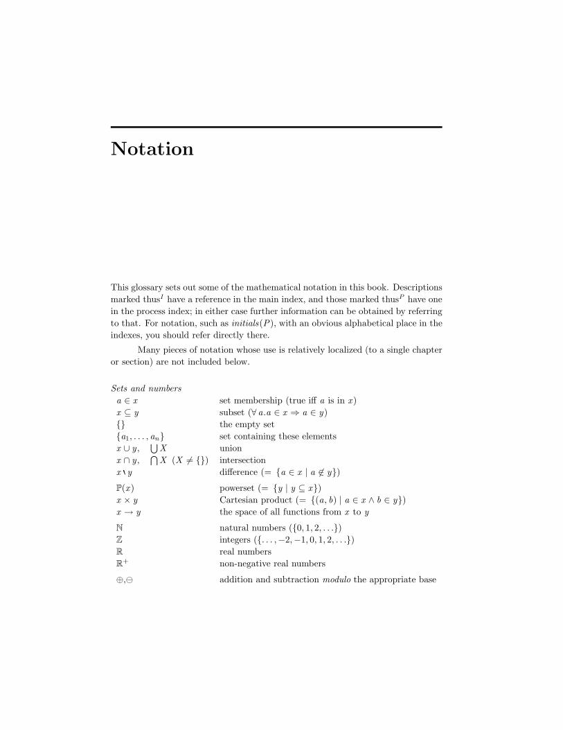
Notation
This glossary sets out some of the mathematical notation in this book. Descriptionsmarked thusI have a reference in the main index, and those marked thusP have onein the process index; in either case further information can be obtained by referringto that. For notation, such as initials(P), with an obvious alphabetical place in theindexes, you should refer directly there.
Many pieces of notation whose use is relatively localized (to a single chapteror section) are not included below.
Sets and numbersa ∈ x set membership (true iff a is in x )x ⊆ y subset (∀ a.a ∈ x ⇒ a ∈ y) the empty seta1, . . . , an set containing these elementsx ∪ y ,
⋃X union
x ∩ y ,⋂
X (X = ) intersectionx y difference (= a ∈ x | a ∈ y)P(x ) powerset (= y | y ⊆ x)x × y Cartesian product (= (a, b) | a ∈ x ∧ b ∈ y)x → y the space of all functions from x to y
N natural numbers (0, 1, 2, . . .)Z integers (. . . ,−2,−1, 0, 1, 2, . . .)R real numbersR
+ non-negative real numbers
⊕, addition and subtraction modulo the appropriate base

564 Notation
Logic
x ∧ y conjunction (x and y)x ∨ y disjunction (x or y)¬x negation (not x )x ⇒ y implication (≡ (¬x ∨ y))x ⇔ y double implication ((x ⇒ y) ∧ (y ⇒ x ))∀ x .χ universal quantification (χ holds for all x )∃ x .χ existential quantification (χ holds for at least one x )
CommunicationsΣ (SigmaI ): alphabet of all communications (tick) terminationI signalτ (tauI ): the invisible actionΣ Σ ∪ Σ,τ Σ ∪ , τa.b.c compound event (see page 26)c?x inputI
c!e outputI
| a, b | events associated with channels (see page 27)
Sequence/trace notation (see pages 36 and 43)
A∗ set of all finite sequences over AA∗ A∗ ∪ s 〈〉 | s ∈ A∗Aω set of all infinite sequences over A
〈〉 the empty sequence〈a1, . . . , an〉 the sequence containing a1,. . . , an in that orders t concatenation of two sequencess \ X hiding: all members of X deleted from ss X restriction: s \ (Σ X )#s length of ss ↓ a (if a is an event) number of a’s: #(s a)s ↓ c (c a channel) sequence of values communicated on c in s
s ≤ t (≡ ∃ u.s u = t) prefix orders ‖
Xt (⊆ Σ∗) generalized parallelI
s ||| t (⊆ Σ∗) interleavingI
S closureI of S (= S ∪ u ∈ Σω | ∀ s < u.s ∈ S)Note that sequence-like notation is also used to denote vectors indexed by arbitrarysets, usually with reference to mutual recursion, for example 〈B∞
s | s ∈ T ∗〉.

Notation 565
Processes
For machine-readable CSP, see Appendix B.
µ p.P recursionI
a → P prefixingI
?x : A→ P prefix choiceI
(a → P | b → Q) guarded alternativeI
P Q external choiceI
P Q , S nondeterministic choiceI
P<I b>I Q conditional choiceI
P ‖ Q synchronous parallelI
P X ‖Y Q alphabetized parallelI
P ‖X
Q generalized parallelI
P ||| Q interleavingI
P \ X hidingI
f [P ] renamingI (functional)P [[R]] renamingI (relational)P [[a/b]] renamingI (relational, by substitution)a.P process namingI
P ; Q sequential compositionI
P >>Q pipingI (or chaining)P//XQ enslavementI
P//m : Q enslavementI (of a named process)P Q ‘time-out’ operator (sliding choice)I
P a Q interruptI
P [x/y ] substitution (for a free identifier x )P/s ‘after’I operatorP ↓ n restrictionI to depth n (model dependent)
LH (P) lazy abstractionI
EH (P) eager abstractionI
MSH (P) mixed abstractionI

566 Notation
Transition systems (see Section 7.2)
C The set of nodes in transition system C .P a−→ Q (a ∈ Σ,τ ) single action transitionP s=⇒ Q (s ∈ Σ∗) multiple action transition with τ ’s removedP t−→ Q (t ∈ (Στ )∗) multiple action transition with τ ’s retained
τ∗(P) (Q | P 〈〉=⇒ Q) τ -expansion of P (see page 545)
P ref B P refuses BP div P diverges
Semantic modelsT traces modelI
N failures/divergences modelI
F stable failures modelI
I infinite traces/divergences modelI
U failures/divergences/infinite traces modelI
⊥N (etc.) bottom elements of modelsP
F (etc.) top elements of modelsP
T traces refinementFD failures/divergences refinementF failures refinement (i.e., over F)I refinement over IU refinement over U refinement over whatever model is clear from the context
(with a special meaning in parts of Chapter 12, and witha default of FD)
P ≤ Q strong orderI (over N or U)
D set of deterministicI processesT d possibly deterministic members of T (see page 222)
Partial orders⊔X least upper boundX greatest lower boundµ f least fixed point of f

Bibliography
[1] L. Aceto and M. Hennessy, Termination, deadlock and divergence, Proceedings ofMFPS89, Springer LNCS 442, 1989.
[2] P.G. Allen, A comparison of non-interference and non-deducibility using CSP, Pro-ceedings of the 1991 IEEE Computer Security Workshop, IEEE Computer SocietyPress, 1991.
[3] R. Alur and T. Henzinger, Logics and models of real time: a survey, in ‘Real time:theory in practice’ (de Bakker et al, eds), Springer LNCS 600, 1992.
[4] K.R. Apt and D.C. Kozen, Limits for automatic verification of finite-state concurrentsystems, 307–309, Information Processing Letters 22, 6, 1986.
[5] G. Barrett, The fixed-point theory of unbounded nondeterminism, Formal Aspects ofComputing, 3, 110–128, 1991.
[6] G. Barrett and M.H. Goldsmith, Classifying unbounded nondeterminism in CSP, in‘Topology and category theory in computer science’ (Reed, Roscoe and Wachter,eds), Oxford University Press, 1991.
[7] G. Barrett and A.W. Roscoe, Unbounded nondeterminism in CSP, Proceedings ofMFPS89, Springer LNCS 442, 1991.
[8] J.D. Beasley, The ins and outs of peg solitaire, Oxford University Press, 1985.
[9] J.A. Bergstra and J.W. Klop, Process algebra for synchronous communicaction, In-formation and Control, 60, 109–137, 1984.
[10] J.A. Bergstra and J.W. Klop, Algebra for communicating processes with abstraction,Theoretical Computer Science, 37, 1, 77–121, 1985.
[11] R.S. Bird, Introduction to functional programming using Haskell, second edition,Prentice Hall, 1998.
[12] S.R. Blamey, The soundness and completeness of axioms for CSP processes, in‘Topology and category theory in computer science’ (Reed, Roscoe and Wachter,eds), Oxford University Press, 1991.

568 Bibliography
[13] P.J. Broadfoot and A.W. Roscoe, Embedding agents within the intruder model todetect parallel attacks, Journal of Computer Security, 12, 2004.
[14] N.A. Brock and D.M. Jackson, Formal verification of a fault tolerant computer,Proceedings of 1992 Digital Aviation Systems Conference, IEEE Computer SocietyPress, 1992.
[15] S.D. Brookes, A model for communicating sequential processes, Oxford UniversityD.Phil thesis, 1983. (Published as a Carnegie-Mellon University technical report.)
[16] S.D. Brookes, Fair communicating processes, in ‘A classical mind: essays in honourof C.A.R. Hoare’, Prentice Hall, 1994.
[17] S.D. Brookes, The essence of Parallel Algol, Proceedings of the 11th IEEE LICS,1996.
[18] S.D. Brookes, C.A.R. Hoare and A.W. Roscoe, A theory of communicating sequentialprocesses, Journal of the ACM 31, 3, 560–599, 1984.
[19] S.D. Brookes and A.W. Roscoe, An improved failures model for CSP, Proceedingsof the Pittsburgh seminar on concurrency, Springer LNCS 197, 1985.
[20] S.D. Brookes and A.W. Roscoe, Deadlock analysis in networks of communicatingprocesses, in ‘Logics and models of concurrent systems’ (K.R. Apt, ed.) NATO ASIseries F, Vol. 13, Springer, 1985.
[21] S.D. Brookes and A.W. Roscoe, Deadlock analysis in networks of communicatingprocesses, Distributed Computing, 4 209–230, 1991.
[22] S.D. Brookes, A.W. Roscoe and D.J. Walker, An operational semantics for CSP,Technical report, 1988.
[23] J.R. Burch, E.M. Clarke, K.L. McMillan, D.L. Dill and L.J. Hwang, Symbolic modelchecking: 1020 states and beyond, 142–170, Information and Computation 98, 2,1992.
[24] E.M. Clarke, R. Enders, T. Filkorn and S. Jha, Exploiting symmetry in temporallogic model checking, Formal Methods in System Design, 9, 77–104, 1996.
[25] G. Colouris, J. Dollimore and T. Kindberg, Distributed systems, concepts and design,Addison-Wesley, 1994.
[26] S. Creese and A.W. Roscoe, Verifying an infinite family of inductions simultane-ously using data independence and FDR, Proceedings of Formal Description Tech-niques for Distributed Systems and Communication Protocols and Protocol Spec-ification, Testing and Verification (FORTE/PSTV’99), October 5-8 1999, Beijing,China. Published by Kluwer Academic Publishers.
[27] S. Creese and A.W. Roscoe Data independent induction over stuctured networks,Proceedings of PDPTA2000
[28] N. Dathi, Deadlock and deadlock-freedom, Oxford University D.Phil thesis, 1990.
[29] J.W.M. Davies, Specification and proof in real-time CSP, Cambridge UniversityPress, 1993.

Bibliography 569
[30] J.W.M. Davies, D.M. Jackson, G.M. Reed, A.W. Roscoe and S.A. Schneider, TimedCSP: theory and applications, in ‘Real time: theory in practice’ (de Bakker et al,eds), Springer LNCS 600, 1992.
[31] J.W.M. Davies and S.A. Schneider, A brief history of Timed CSP, Oxford UniversityComputing Laboratory technical monograph PRG-96, 1992.
[32] R. de Nicola and M. Hennessy, Testing equivalences for processes, Theoretical Com-puter Science 34, 1, 83–134, 1987.
[33] E.W. Dijkstra and C.S. Scholten, A class of simple communication patterns, in‘Selected writings on computing’, EWD643, Springer-Verlag, 1982.
[34] E.A. Emerson and A.P. Sistla, Utilizing symmetry when model checking under fair-ness assumptions: an automata-theoretic approach, 309–324, Proceedings of the 7th
CAV, Springer LNCS 939, 1995.
[35] E.A. Emerson and A.P. Sistla, Symmetry and model checking, Formal Methods inSystem Design, 9, 105–131, 1996.
[36] H.B. Enderton, Elements of set theory, Academic Press, 1977.
[37] R. Focardi and R. Gorrieri, Comparing two information-flow properties, Proceedingsof 1996 IEEE Computer Security Foundations Workshop, IEEE Computer SocietyPress, 1996.
[38] R. Forster, Non-interference properties for nondeterministic systems, Oxford Uni-versity D.Phil. thesis, 1999.
[39] Formal Systems (Europe) Ltd, Failures-Divergence Refinement: FDR2 Manual,1997.
[40] N. Francez, Fairness, Springer, 1986.
[41] , H. Garcia-Molina, Elections in a distributed computing system, IEEE transactionson Computers, January 1982.
[42] S. Graf, Verification of a distributed cache memory by using abstractions, Proceed-ings of the 6th CAV, Springer LNCS 818, 1994.
[43] S. Graf and B. Steffen, Compositional minimisation of finite-state systems, Proceed-ings of CAV ’90, Springer LNCS 531, 1990.
[44] J.C. Graham-Cumming, The formal development of secure systems, Oxford Univer-sity D.Phil thesis, 1992.
[45] I. Guessarian, Algebraic semantics, Springer LNCS 99, 1981.
[46] F. Harary, Graph theory, Addison-Wesley, 1969.
[47] He Jifeng and C.A.R. Hoare, From algebra to operational semantics, InformationProcessing Letters, 46, 2, 1993.
[48] He Jifeng, C.A.R. Hoare and A. Sampaio, Normal form approach to compiler design,Acta Informatica, 30, 701–739, 1993.

570 Bibliography
[49] C.L. Heitmeyer and R.D. Jeffords, Formal specification and verification of real-timesystem requirements: a comparison study, U.S. Naval Research Laboratory technicalreport, 1993.
[50] A. Hojati and R.K. Brayton, Automatic datapath abstraction in hardware systems,98–113, Proceedings of the 7th CAV, Springer LNCS 939, 1995.
[51] M. Hennessy, Algebraic theory of processes, MIT Press, 1988.
[52] M. Hennessy and H. Lin, Symbolic bisimulations, 353–389, Theoretical ComputerScience, 138, 2, 1995.
[53] M.G. Hinchey and S.A. Jarvis, Concurrent systems: formal development in CSP,McGraw-Hill, 1995.
[54] C.A.R. Hoare, Communicating sequential processes, Communications of the ACM,21, 8, 666–677, 1978.
[55] C.A.R. Hoare, A model for communicating sequential processes, in ‘On the construc-tion of programs’ (McKeag and MacNaughten, eds), Cambridge University Press,1980.
[56] C.A.R. Hoare, Communicating sequential processes, Prentice Hall, 1985.
[57] Inmos Ltd., occam2 reference manual, Prentice Hall, 1988.
[58] C.N. Ip and D.L. Dill, Better verification through symmetry, Formal Methods inSystem Design, 9, 41–75, 1996.
[59] K. Jensen, Condensed state spaces for symmetrical coloured Petri nets, Formal Meth-ods in System Design, 9, 7–40, 1996.
[60] G. Jones and M.H. Goldsmith, Programming in occam2, Prentice Hall, 1988.
[61] B. Jonsson and J. Parrow, Deciding bisimulation equivalences for a class of non-finite-state programs, Information and Computation 107, 2, 272–302, 1993.
[62] A. Jung, ed, Domains and denotational semantics: history, accomplishments andopen problems, 1996.
[63] P.C. Kanellakis and S.A. Smolka, CCS expressions, finite state processes and threeproblems of equivalence, Information and Computation 86, 43–68, 1990.
[64] R.S. Lazic, A semantic study of data-independence with applications to the mechan-ical verification of concurrent systems, Oxford University D.Phil thesis, to appearin 1997.
[65] R.S. Lazic, Theorems for mechanical verification of data-independent CSP, OxfordUniversity Computing Laboratory technical report, 1997.
[66] R.S. Lazic, T. Newcomb and A.W. Roscoe, Polymorphic Systems with Arrays, 2-Counter Machines and Multiset Rewriting, Proceedings of INFINITY 2004.
[67] R.S. Lazic and A.W. Roscoe, Using logical relations for automated verification ofdata-independent CSP, Proceedings of the Workshop on Automated Formal Methods(Oxford, U.K.), Electronic Notes in Theoretical Computer Science 5, 1997.

Bibliography 571
[68] R.S. Lazic and A.W. Roscoe, A study of data-independence in CSP, Submitted forpublication, 1997.
[69] N.G. Leveson and J.L. Stolzy, Analyzing safety and fault tolerance using timed Petrinets, Proceedings of TAPSOFT, Springer, 1985.
[70] G. Lowe, Pravda: a tool for verifying probabilistic processes, Proceedings of theWorkshop on Process Algebra and Performance Modelling, 1993.
[71] G. Lowe, Breaking and fixing the Needham-Schroeder public-key protocol using FDR,Proceedings of TACAS ’96, Springer LNCS 1055, 1996.
[72] G. Lowe, Some new attacks upon security protocols, Proceedings of 1996 IEEE Com-puter Security Foundations Workshop, IEEE Computer Society Press, 1996.
[73] G. Lowe, Casper: a compiler for the analysis of security protocols, Proceedingsof 1997 IEEE Computer Security Foundations Workshop, IEEE Computer SocietyPress, 1997.
[74] G. Lowe, Towards a completeness result for model checking of security protocols,ournal of Computer Security, Volume 7, Numbers 2, 3, pages 89-146, 1999. An ear-lier version appeared in Proceedings of 11th IEEE Computer Security FoundationsWorkshop, pages 96-105, 1998.
[75] G. Lowe and A.W. Roscoe, Using CSP to detect errors in the TMN protocol, Uni-versity of Leicester Dept. of Mathematics and Computer Science technical report1996/34, and to appear in the Journal of Computer Security.
[76] W.F. McColl, Scalable computing, in ‘Computer science today: recent trends anddevelopments’, Springer LNCS 1000, 1995.
[77] K. McMillan, Symbolic model checking, Kluwer Academic Publishers, 1993.
[78] J.M.R. Martin, The design and construction of deadlock-free concurrent systems,University of Buckingham D.Phil thesis, 1996.
[79] R. Milner, Fully abstract models of typed lambda-calculi, Theoretical Computer Sci-ence 4, 1–22, 1977.
[80] R. Milner, A calculus of communicating systems, Springer LNCS 92, 1980.
[81] R. Milner, Lectures on a calculus for communicating systems, Proceedings of thePittsburgh seminar on concurrency, Springer LNCS 197, 1985.
[82] R. Milner, Communication and concurrency, Prentice Hall, 1989.
[83] R. Milner, J. Parrow and D. Walker, A calculus of mobile processes, I and II, Infor-mation and Computation 100, 1, 1–77, 1992.
[84] M.W. Mislove, A.W. Roscoe and S.A. Schneider, Fixed points without completeness,Theoretical Computer Science 138, 2, 273–314, 1995.
[85] J.J. Mitchell, Type systems for programming languages, in ‘Handbook of theoreticalcomputer science’ (van Leeuwen, ed), Elsevier, 1990.
[86] Mukkaram, A., A refusal testing model for CSP, Oxford University D.Phil thesis,1993.

572 Bibliography
[87] E.R. Olderog and C.A.R. Hoare, Specification-oriented semantics for communicatingprocesses, Acta Informatica, 23, 9–66, 1986.
[88] J. Ouaknine, Discrete analysis of continuous behaviour in real-time concurrent sys-tems, Oxford University D.Phil thesis, 2001.
[89] D. Park, On the semantics of fair parallelism, in ‘Abstract software specifications’(Bjorner, ed), Springer LNCS 86, 1980.
[90] W.W. Peterson and E.J. Weldon, Jr., Error-correcting codes, M.I.T. Press, 1972.
[91] Phillips, I., Refusal testing, Theoretical Computer Science 50 pp241–284 (1987).
[92] G.D. Plotkin, LCF considered as a programming language, Theoretical ComputerScience 5, 223–255, 1977.
[93] G.D. Plotkin, Lambda-definability in the full type hierarchy, in ‘To H.B. Curry: es-says on combinatory logic, lambda calculus and formalism’ (Seldin and Hindley,eds), Academic Press, 1980.
[94] G.D. Plotkin, A structured approach to operational semantics, DAIMI FN–19, Com-puter Science Dept., Aarhus University, 1981.
[95] A. Pnueli and E. Shahar, A platform for combining deductive with algorithmic veri-fication, 184–195, Proceedings of the 8th CAV, Springer LNCS 1102, 1996.
[96] D.K. Probst and H.F. Li, Using partial order semantics to avoid the state explosionproblem in asynchronous systems, Proceedings of CAV ’90, Springer LNCS 531,1990.
[97] G.M. Reed, A uniform mathematical theory for real-time distributed computing, Ox-ford University D.Phil thesis, 1988.
[98] G.M. Reed and A.W. Roscoe, A timed model for communicating sequential processes,Theoretical Computer Science 58, 249-261, 1988.
[99] G.M. Reed and A.W. Roscoe, Analysing TMFS : a study of nondeterminism in real-time concurrency, in ‘Concurrency: theory, language and architecture’ (Yonezawaand Ito, eds), Springer LNCS 491, 1991.
[100] J.C. Reynolds, Types, abstraction and parametric polymorphism, Information Pro-cessing 83, 513–523, North-Holland, 1983.
[101] A.W. Roscoe, A mathematical theory of communicating proceses, Oxford UniversityD.Phil thesis, 1982.
[102] A.W. Roscoe, Denotational semantics for occam, Proceedings of the Pittsburghseminar on concurrency, Springer LNCS 197, 1985.
[103] A.W. Roscoe, Routing messages through networks: an exercise in deadlock avoid-ance, Proceedings of 7th occam User Group technical meeting, IOS B.V., Amster-dam, 1987.
[104] A.W. Roscoe, An alternative order for the failures model, in ‘Two papers on CSP’,technical monograph PRG-67, Oxford University Computing Laboratory, July 1988.Also Journal of Logic and Computation 2, 5, 557–577, 1992.

Bibliography 573
[105] A.W. Roscoe, Unbounded nondeterminism in CSP, in ‘Two papers on CSP’, techni-cal monograph PRG-67, Oxford University Computing Laboratory, July 1988. AlsoJournal of Logic and Computation, 3, 2 131–172, 1993.
[106] A.W. Roscoe, Maintaining consistency in distributed databases, Oxford UniversityComputing Laboratory technical monograph PRG-87, 1990.
[107] A.W. Roscoe, Topology, computer science and the mathematics of convergence, in‘Topology and category theory in computer science’ (Reed, Roscoe and Wachter,eds), Oxford University Press, 1991.
[108] A.W. Roscoe, Model checking CSP, in ‘A classical mind: essays in honour of C.A.R.Hoare’, Prentice Hall, 1994.
[109] A.W. Roscoe, CSP and determinism in security modelling, Proceedings of 1995 IEEESymposium on Security and Privacy, IEEE Computer Society Press, 1995.
[110] A.W. Roscoe, Modelling and verifying key-exchange protocols using CSP and FDR,Proceedings of 1995 IEEE Computer Security Foundations Workshop, IEEE Com-puter Society Press, 1995.
[111] A.W. Roscoe, Intensional specifications of security protocols, Proceedings of 1996IEEE Computer Security Foundations Workshop, IEEE Computer Society Press,1996.
[112] A.W. Roscoe, Finitary refinement checks for infinitary specifications, Proceedingsof CPA 2004.
[113] A.W. Roscoe, Proving security protocols with model checkers by data independencetechniques, Proceedings of CSFW 1998.
[114] A.W. Roscoe, Seeing beyond divergence, Proceedings of “25 Years of CSP”, LNCS3525 (2005).
[115] A.W. Roscoe, On the expressiveness of CSP refinement, to appear in FAC.
[116] A.W. Roscoe, Revivals, stuckness and responsiveness, to appear, 2005
[117] A.W. Roscoe and P.J. Broadfoot, Proving security protocols with model checkersby data independence techniques, (expanded version of [113]) Journal of ComputerSecurity 7, 1999.
[118] A.W. Roscoe and N. Dathi, The pursuit of deadlock freedom, Information and Com-putation 75, 3, 289–327, 1987.
[119] A.W. Roscoe, P.H.B. Gardiner, M.H. Goldsmith, J.R. Hulance, D.M. Jackson andJ.B. Scattergood, Hierarchical compression for model-checking CSP or how to check1020 dining philosophers for deadlock, Proceedings of the 1st TACAS, BRICS NotesSeries NS-95-2, Department of Computer Science, University of Aarhus, 1995. (AlsoSpringer LNCS 1019.)
[120] A.W. Roscoe and M.H. Goldsmith, The perfect ‘spy’ for model-checking crypto-protocols, Proceedings of DIMACS workshop on the design and formal verificationof cryptographic protocols, 1997.

574 Bibliography
[121] A.W. Roscoe and C.A.R. Hoare, The laws of occam programming, Theoretical Com-puter Science, 60, 177-229, 1988.
[122] A.W. Roscoe and H. MacCarthy, Verifying a replicated database: A case study inmodel-checking CSP, Formal Systems technical report, 1994.
[123] A.W. Roscoe, J.C.P. Woodcock and L. Wulf, Non-interference through determin-ism, Journal of Computer Security 4, 1, 27–54, 1996 (revised from Proceedings ofESORICS 94, Springer LNCS 875).
[124] A.W. Roscoe and L. Wulf, Composing and decomposing systems under security prop-erties, Proceedings of 1995 IEEE Computer Security Foundations Workshop, IEEEComputer Society Press, 1995.
[125] P.Y.A. Ryan, A CSP formulation of non-interference, Cipher, 19–27. IEEE Com-puter Society Press, 1991.
[126] J.B. Scattergood, Tools for CSP and Timed CSP, Oxford University D.Phil thesis,forthcoming 1997.
[127] S.A. Schneider, Correctness and communication in real-time systems, Oxford Uni-versity D.Phil thesis, 1989.
[128] W.A. Sutherland, Introduction to metric and topological spaces, Oxford UniversityPress, 1975.
[129] H. Tej and B. Wolff, A corrected failure-divergence model for CSP in Isabelle/HOL,To appear in the Proceedings of FME97.
[130] L.G. Valiant, A bridging model for parallel computation, Communications of theACM, 33, 8 103–111, 1990.
[131] A. Valmari, Stubborn sets for reduced state space generation, Proceedings of 10th
International conference on theory and applications of Petri nets, 1989.
[132] A. Valmari, The weakest deadlock-preserving congruence, Information ProcessingLetters 53, 341–346, 1995.
[133] A. Valmari and M. Tienari An improved failures equivalence for finite-state sys-tems with a reduction algorithm, Protocol Specification, Testing and Verification XI,North-Holland, 1991.
[134] P.L. Wadler, Theorems for free!, 347–359, Proceedings of the 4th ACM FPLCA,1989.
[135] D.J. Walker, An operational semantics for CSP, Oxford University M.Sc. disserta-tion, 1986.
[136] P.H. Welch, G.R.R. Justo and C.J. Willcock, High-level paradigms for deadlock-freehigh-performance systems, Transputer Applications and Systems ’93, IOS Press,1993.
[137] P. Wolper, Expressing interesting properties of programs in propositional temporallogic, 184–193, Proceedings of the 13th ACM POPL, 1986.
Bibliography 575
[138] L. Wulf, Interaction and security in distributed computing, Oxford University D.Philthesis, 1997.
[139] J.T. Yantchev, ARC – A tool for efficient refinement and equivalence checking forCSP, IEEE 2nd Int. Conf. on Algorithms and Architectures for Parallel Processing,1996.
[140] J.T. Yantchev and C.R. Jesshope, Adaptive, low latency, deadlock-free packet routingfor processor networks, IEE Proc. E, May 1989.
[141] I. Zakiuddin, An FDR analysis of a fault-tolerant information system, Proceedingsof AAS ’97, ACM, 1997.
How to obtain the tools mentioned in this book
The following details are believed to be correct at the time of writing, but potentialusers are advised in the case of difficulty to consult the web site given in the Preface.The web site should also contain details of further tools.
• FDR: this is a product of Formal Systems (Europe) Ltd. At the time ofwriting the release is 2.11. Much of what is described in this book does notapply to the earlier FDR 1. For details please email [email protected].
• ProBE: at the time of writing this animator is under beta-test by FormalSystems (Europe) Ltd, with a formal release expected later in 1997. Fordetails please email [email protected].
• Jeremy Martin’s Deadlock Checker (see Section 13.6) operates (at the time ofwriting) on the more restricted syntax used by FDR 1. It is hoped to rectifythis. You can obtain it through the web site with URL
http://users.ox.ac.uk/~jeremy/Deadlock/index.html
• Gavin Lowe’s Casper (a security protocol compiler, as discussed in Section15.4) can be obtained through the web site with URL
http://www.mcs.le.ac.uk/~gl7/Security/Casper/index.html


Main index
Entries in bold face are the primary reference(s) to the item concerned, while italicentries denote references in exercises. Note that processes have a separate index,following this one.
abstraction, 24, 82, 89, 295–328, 364,376–378, 532
eager, 296, 400, 428lazy, 297–327, 400, 407, 412, 428mixed, 302–305, 326, 387, 401, 428,
538over T (hiding), 296, 306
acceptance sets, 278, 522, 530acknowledgement messages, 128ACP, 269actions
invisible (τ), 48, 77, 78, 80, 92, 136,160, 178, 410, 463, 530
visible, see communications‘after’ operator (P/s), 47algebraic semantics, 29–35, 39, 149, 269–
293, 517alphabet, 13
process, 55, 76transformation, see renaming
alphabetized parallel (X ‖Y ), 55–65, 380as conjunction of trace specifications,
70–74, 333, 396in terms of ‖
X, 68, 70
indexed, 57laws of, 57, 82, 88, 142, 276termination of, 139traces of, 60with intrinsic alphabets, 76
alternating bit protocol, 128–133, 211–213, 221, 259, 309–311, 358, 403–409, 533
animator, 48articulation point, 372ASCII version of CSP, see machine-readable
CSPATM (Automated Teller Machine), see
cash-point machinesattack (on a crypto-protocol), 449, 450,
455, 460, 461, 464, 465authentication, 446, 447, 460axiom, 229
D1, 192, 204, 207, 246D2, 192, 198, 204, 207, 246D2′, 246D3, 192, 196, 246D4, 246F1, 192F2, 192
578 Main index
F3, 192, 219, 251F4, 192, 198I1, 253I1′, 246I2, 254T1, 208, 246T2, 208T3, 208
axiom of choice, 474
bag, 67, 124Banach’s theorem, see contraction map-
ping theoremBarrett, Geoff, 256–257, 268biconnected components, 372binary decision diagram (BDD), 529binary switching network, 363–364, 378bisimulation, 154–158, 284, 521, 522,
529Blamey, Stephen, 268breadth-first search (BFS), 527–528Brookes, Stephen, 178, 214, 292, 380BSP (Bulk Synchronous Parallelism), 5buffer, 18, 78, 81, 85, 103, 113–134
characteristic process, 115failures/divergences specification of,
114infinite, 18, 103, 188laws, 116–121, 125–126, 207specification is infinite state, 50tolerance, 125–128, 133, 430trace specification of, 43, 46, 104,
113weak, 116
busy network, 334, 371, 378Byzantine failure, 312
cache, 465coherency, 441–446miss, 442replacement policy, 442
cash-point machines, 20–21, 24, 28, 53–54, 55, 63–64, 65, 68, 82–83,388, 409
Casper, 461, 550Cauchy sequence, 490CCS, 5, 154, 178, 214, 536chain, 473chaining, see pipingchannels, 18, 26, 27, 99, 334, 376
arrays of, 27, 63conflict-free, 339internal and external, 58, 77type discipline restricts practicality
of >> and //, 110Chaos , 29, 42, 214, 299, 309, 312, 314,
323–324, 428is non-divergent, 83
characteristic process, 46, 65, 97, 115chase(P), 462–464, 531choice
conditional, see conditional choiceexternal, see external choiceguarded, see guarded alternativenondeterministic, see nondetermin-
istic choicesliding, see ‘time-out’ operator
client/server networks, 347closed CSP term, 159closed set, 489–490closure of trace set, 172combinatorial exploration, 416, 422comms(e), 160communication graph, 58, 62, 335, 342,
343, 353, 362, 370, 533communication media, 320
insecure, 446unreliable, 103, 104, 118, 129–130,
212, 260, 309–310, 404communications, 8–10, 13, 20–21
agreement with environment on, 13,152
are instantaneous, 13multi-part, 17, 26
communications protocols, 102, 113, 128,211
layering of, 103completeness of a set of laws, 270

Main index 579
compositional development, 46, 533compression of state spaces, 306, 307, 378,
463, 525, 528–538inapplicable with priority, 412
concurrency, theory of, 1concurrent systems, 1conditional choice, 25–26, 49
for collapsing case definitions, 25laws of, 30–34
confidentiality, 446, 460configurations, 520conflict, 337–339, 341, 364
freedom from, 337, 341, 344, 347,349, 350, 360, 371
congruence, 180–181, 200, 238, 269consistency (of distributed data), 423–
430constraints via parallel composition, 71,
72, 131, 420–422constructiveness, 39, 53, 84–85, 103, 122–
123, 186–189, 196, 203, 206,220, 225, 250, 266–267, 493
contexts, 46, 180, 208, 228, 232–238, 412continuity, 184–186, 204–206, 206, 211,
476–478, 481, 483–485disappears with unbounded nonde-
terminism, 248of predicates, 225
contraction map, 491–494contraction mapping theorem, 181, 224–
225, 491–494convergence, 473, 488covert channel, 317
timing, 323cpo, see partial order, completecritical regions, 308crypto-protocols, 446–466CSP (1978 version), 5CSP, modern version, 5cycle of ungranted requests, 336–379cycle-cutting set, 362cyclic communication network, 349–353,
358, 360, 362, 366–367, 379, 536generalized, 350
data structures implemented as networks,107
data type, 17, 27, 430–440data types for symbolic encryption, 449data-independence, 295, 376, 423, 430–
440, 443–446, 464, 533weak, 434
Dathi, Naiem, 380Davies, J.W.M. (Jim), 413de Nicola, Rocco, 214deadlock, 3, 10, 62, 65, 131, 180, 234–
238, 306, 331–382, 428compression in checking, 533failures specification of deadlock free-
dom, 97fundamental principle of, 342, 343,
347, 365, 371hereditary deadlock freedom, 373–
375is static, 332, 335represented by STOP , 54Rule 1, 342, 370, 373Rule 2, 344, 345, 346, 358, 361, 372,
373, 377Rule 3, 347, 348, 358, 372, 373Rule 4, 349, 358, 360, 372, 373, 380Rule 5, 349, 351, 372, 373Rule 6, 351, 352, 373Rule 7, 354, 355, 372, 373Rule 8, 357, 365, 373, 425, 427Rule 9, 359, 360, 361, 364, 372, 373,
379Rule 10, 362, 364, 372, 373Rule 11, 365, 373Rule 12, 366, 367Rule 13, 371Rule 14, 371Rule 15, 377Rule 4, 358Rule 5, 358state, 335–338, 340–341
Deadlock Checker, 378–379, 550declarative semantics, 19, 136, 138, 150deductions(X), 456

580 Main index
denotational semantics, 149, 179–216,517
denseness, 228depth-first search (DFS), 526, 527, 530derived operator, 99det(P), 219, 254, 255determinism, 3, 23, 96, 97, 194, 204, 217–
222, 243, 252, 257, 258, 299–301, 305, 312, 316–328, 439–440, 463
algorithm for deciding, 222FDR as a checker of, 325over F , 217, 325, 440
diamond elimination, 530, 531diamond(P), 530Dijkstra, E.W., 380dining philosophers, 3, 60–63, 65, 67,
86, 338–339, 353–355compression of, 532, 533
directed set, 184, 194, 195, 205, 473, 482,490
disconnecting edge, 370–372distributed database, 423–430, 464distributed termination, 139–140, 142,
178operational semantics of, 164
distributivity (over ), 30, 54, 183–184,202–203, 206
div, 83, 96, 135, 209laws of (over N ), 275–276laws of (over T and F), 290
divergences, 3, 10, 83, 92–98, 130, 131,137, 161, 170, 191, 195, 204,209, 236–238, 428, 522, 526
in timed processes, 398seeing past, 207, 211strictness after, 95, 172, 192, 193,
200, 204, 205, 207, 276divergences(P), 95, 191, 192
calculation of, 197–202divide and conquer, 108dynamic networks, 103, 107, 188, 332,
342usually infinite state, 110
encryption, 446, 455, 465algebraic identities over, 461public-key, 447, 448, 452symbolic representation of, 449symmetric, 447, 452
enslavement (//), 105–111, 138, 342, 441builds tree networks, 107
environment (external), 13, 24, 145, 387environment (semantic), 160, 239error correcting codes, 128error correction, 119essential component, 370–372Events, 49events
invisible, see actions, invisiblevisible, see communications
events(c), 27eventuality, 264explicate(P), 528, 531explode(P), 456expressibility, 229–232, 253external choice, 22–23, 94, 183, 206
ambiguous initial events, 23laws of, 30–34, 86, 90, 141, 276operational semantics of, 161
fact (data type for encryption), 449failure modes, 312failures, 92–98, 192, 251, 398
stable, 191, 207–214failures(P), 92, 171, 246
calculation of, 210failures⊥(P), 95, 171, 191, 192
calculation of, 197–202failures/divergences model (N ), 95, 144–
145, 191–207, 209, 214, 217–219, 255, 275, 522, 526
applicability of, 200, 231expressibility of elements, 231–232full abstraction, 235–237lazy abstraction over, 297normal forms for, 281–285
failures/divergences/infinite traces model(U), 245–268, 303

Main index 581
lazy abstraction over, 298–299, 305Fair(A,B), 259fairness, 131, 259–266fault tolerance, 309–316, 325, 409, 435
abstract definition of, 314of replicated processor, 312
FDR, xi, 7, 48–50, 60, 97, 98, 306, 325,375, 413, 415–466, 517–538,550
compiler, 519finite state machine, see state machine,
transition systemfixed point induction, 124, 134, 223–226,
250, 266–267fixed points, 38, 84, 158, 181, 196, 223–
228, 471–479, 491for mutual recursions, 38positive and negative, 190, 203–204
fixed-point induction, 122–123, 181FOR loop, 138formats, see configurationsfull abstraction, 180, 228–238, 243, 253–
255, 289, 291affected by adding operators, 235
function, 89injective, 87spaces, 483–485strict, 472
functional programming language, 19, 150,415, 495–515
game theory, 254generalized parallel (‖
X), 68–70
laws of, 69, 82, 88, 142, 276, 288traces of, 69, 144
Gofer, 495greatest lower bound, 193, 209, 246, 255,
469–471, 481guarded alternative, 15–17, 18, 22, 49
representable using , 22guardedness, see constructiveness
halting problem, 135, 277, 430
handshaken communication, 5, 6, 9, 20,51, 71, 126
Haskell, 19, 495Hasse diagram, 468He, Jifeng, 293head normal form (hnf), 271–277, 278,
282, 285, 287, 289, 291, 292Hennessy, Matthew, 214hiding, 77–86, 199–202, 333, 380, 532
never hidden, 140continuity over N , 205discontinuous over T , 184, 190divergences of over U and I, 247infinite, 83, 176laws of, 78–82, 88, 141, 276, 288negates guardedness, 84operational semantics of, 162traces of, 83
high level implementation, 518hnf, see head normal formHoare, C.A.R. (Tony), xi, 5, 43, 76, 140,
214, 293, 302
identifiersnon-process, 25, 37, 159
binding of, 19, 34change of, 272scope of, 136
process, 14, 161, 228, 238, 239independence, 317, 327, 465
lazy, 317, 325mixed (or transaction), 317
inductive compression, 536inference system
via parallel composition, 458–464infinite traces/divergences model (I), 246–
250infinites(P), 172
calculation of, 247infix dot, 18, 26initials(P), 47, 193, 278initiator, 451input, 18–19, 27, 99–102, 302, 346, 385,
387

582 Main index
interaction, 2, 51interface parallel, see generalized parallelinterleaving (|||), 65–68
as abbreviation for disjoint parallel,67
as abstraction mechanism, 326in terms of ‖
X, 68
laws of, 66, 142, 276operational semantics of, 169recursion through, 66traces of, 67, 144
internal choice, see nondeterministic choiceinterrupt operator (), 235, 286intruder (spy), 446, 449, 450, 453–461invariant (of a network), 374iteration
parallel, 102sequential, 137
Jackson, David M., 413Jategoankar, Lalita, 216, 243
knowledge, deduction of, 455–464Konig’s lemma, 173, 205, 242, 258
labelled transition system, see transitionsystem
lambda (λ-) calculus, 232lattice, 470
complete, 182, 209, 246, 470–471,473
law, 29, 34, 39, 78, 149, 206, 269, 285,292, 333, 380
associative, 29, 57commutative, 29distributive, 29idempotence, 29step, 32, 79–81symmetry, 29, 57unit, 29zero, 29, 276
Lazic, Ranko, 150, 433, 437, 439, 465lazy spy, 458–464leaf compression, 537
least upper bound, 194, 209, 469–471,481
level crossing, 388–397, 413livelock, see divergencesliveness, see specification, livenesslogical relations, 432, 465low level implementation, 518low-deterministic process, 324Lowe, Gavin, 460, 461, 550lower bound, 469LTS, see transition system
machine-readable CSP, 8, 19, 25, 27, 48–49, 74, 89, 98, 109–111, 415,495–515
Martin, Jeremy, 378–380, 550matrix multiplication network, 351–352,
362–363, 376maximal progress, 410memory device, 303memory model, 441–443mergesort network, 109message-passing ring, 355–357, 425metric spaces, 181, 186–187, 220, 224–
225, 250, 486–494complete, 490
Meyer, Albert, 216, 243Milner, Robin, 5, 536–537model checking, 17, 75, 82, 422, 464, 526model compress(P), 530modular compression, 533monitor, 313, 325monotonicity, 116, 195, 202, 204, 211,
257, 472–479, 481, 483–485and refinement, 46is implied by distributivity, 184
mutual exclusion, 4, 308
Needham–Schroeder Public-Key protocol,447–461
Newton’s method, 102, 104node ordering, 344NoEqT (no equality tests), 433non-Archimedean metric, 488

Main index 583
non-destructiveness, 104, 187, 196, 206,493
non-expanding map, 491–494non-interference, see independencenonce, 448, 455nondeterminism, 2, 10, 23, 24, 152
angelic, 261finite, 23inevitable in concurrency theory, 83introduced by , 219introduced by ‖
X, 220
introduced by abstraction, 24, 296introduced by external choice, 23introduced by hiding, 80, 82, 220introduced by renaming, 89, 220unbounded, 23, 83, 89, 176, 195,
196, 200, 215, 231, 243, 245–268, 299
nondeterministic choice, 23–25, 94, 183,471
fair, 261–262infinite, 176laws of, 30–34, 276operational semantics of, 160
nondeterministic selection ($), 433, 435nondeterministic systems
are untestable, 3Norm (normality conditions), 435, 436normal form, 277–286, 289, 291, 465,
521, 524one-step, 281, 289
normal(P), 529, 533normalization, 281, 306, 432, 517, 521–
525, 529–531can be exponential, 524
occam, 5, 22, 78, 293, 357, 380Olderog, E.-R., 243Ω (Omega): terminated process, 159open set, 489operating system, 4operational semantics, 78, 149–178, 190,
250, 432, 465, 517–521
congruence with denotational seman-tics, 238–243
via algebraic reduction, 271–277,292
order isomorphism, 468output, 18–19, 27, 99–102, 346, 385, 387
as signal events, 302
pantomime horse, 55, 64, 65parallel communication, 350–352parallel computers, 1, 2parallel networks, 331–343parallel processes
can be sequentialized, 52, 58parameterization, 63, 87parameterized verification problem (PVP),
430, 445parameters, process, 19, 49, 150, 430parametricity, 432, 465partial order, 181, 195, 224, 255–257, 344,
467–486bottom (⊥), 468complete (cpo), 194, 195, 473–475maximal element, 468, 474, 479minimal element, 468top (), 468
partial order methods (in model check-ing), 464
philosophers, dining, see dining philoso-phers
piping (>>), 99–105, 109, 116, 207, 342laws of, 100–102, 142traces of, 102
Plotkin, Gordon, 178point-to-point communication, 78, 333polymorphism, 76, 431post-fixed point, 257, 478pre-deterministic process, 256pre-fixed point, 158, 478pre-normal form, 522, 524prefix choice, 17–19, 49prefix order on sequences, 468prefixing, 14
laws of, 30–34

584 Main index
operational semantics of, 159prioritize(P), 413, 531priority, 409–413
limits applicability of denotationalmodels, 411
ProBE, 8, 48–49, 110, 177, 550process algebras, 5, 6, 154, 214, 269process naming (a.P), 87, 98, 105product of partial orders, 480–486projection, 297public key, 447, 450puzzles, 416
quicksort network, 108, 191, 343
railways, 9, 73, 373–375, 388, 416recursion, 14–15, 122, 203, 223–228
and fixed points, 37, 181, 188–190,195, 203, 248–250
equational and µ styles, 15guarded, see constructivenessill-formed, 83, 188–190, 203, 204is not distributive, 31laws of, 34mutual, 14, 38, 41, 59, 122, 480
infinite, 16, 66operational semantics of, 161, 178parameterized, 19, 38, 53, 63, 480tail, see tail recursionthrough sequential composition, 137trace proof rules, 44
reduction strategy, 271Reed, G.M. (Mike), 413refinement, 24, 300
checking, 525–527is PSPACE-hard in worst case,
523failures, 94, 95, 97failures/divergences, 96–98, 203FDR as checker of, 49over U , 255properties of, 46provable algebraically, 47trace, 45, 48, 97, 182, 184
refinement paradox, 324reflexivity, 468refusal set, 92, 93, 171, 192, 204, 207,
215maximal, 93, 231, 278, 279may contain , 145relationship with acceptance sets, 278relationship with infinite traces, 254
refusals(P), 92, 193relation, 89, 182, 468
composition of, 90domain and range of, 89
relational representations of operators, 182–188, 202, 204, 206, 207, 210,254
remote procedure call, 105renaming, 86–92, 333, 380, 453, 460, 461
never affected, 140as an abstraction mechanism, 295,
377–378infinite-to-one, 176injective, 87–88inverse function, 89laws of, 88, 90–91, 141, 276non-injective, 88–89traces of, 91, 143
request, 335, 341selective, 365ungranted, 335–339, 341, 362, 365
resource sharing, 353–355responder, 451restriction space, 186–188, 196, 206, 224–
225, 488complete, 490
routeing algorithms, 344, 348, 363, 376RUN , 29, 42, 47, 265, 306, 309, 326
safety, see specification, safetysat, 43, 46, 47sbisim(P), 529Scattergood, Bryan, 150, 495scheduler ring, 536–537Schneider, Steven, 7, 413Scholten, C.S., 380

Main index 585
SDD, see state dependency digraphsecret key, 447, 450security
information flow, 316–328limitations of CSP models, 323–325protocols, 446–466
semantic equivalence factoring, 530semaphore, 4semi-separable, 325SemiFair(A,B), 265, 298separability, 300–302, 318, 321, 324, 325,
327sequence notation, 36, 43sequential composition (; ), 135–143, 206,
286–290laws of, 140–143, 276operational semantics of, 162traces of, 143, 182, 184
server, 448session, 452session key, 447, 452set process, 107settle time, 409shared-variable concurrency, 4Σ (Sigma), 8, 13, 49, 78Σ, 135signal (undelayable) events, 145, 302–304,
307signal events, 387signature, cryptographic, 447–449SKIP , 135, 286–290
laws of, 140–143, 288operational semantics of, 159traces of, 143
sliding choice, see ‘time-out’ operatorsnapshot graph (of deadlock), 335solitaire, 416–422, 519–520soundness of a set of laws, 270specification
behavioural, 42, 45, 97, 114, 314compression of, 525failures, 95, 97, 306–309, 398, 428failures/divergences, 97, 114infinite state, 115–116
infinite trace, 258–259liveness, 45, 207
timed, 397of a subset of the alphabet, 306–309operators primarily for, 9partial correctness, 45processes as, 9safety, 45, 395, 429, 451
timed, 388–397total correctness, 45trace, 42–47, 48, 65, 66, 97, 115,
306, 536limitations of, 45, 113
untimed of timed process, 398–403spy, see intruderstable failures model (F), 207–216, 217,
246, 306–307, 340, 378, 526, 534applicability of, 211expressibility of elements, 229–230full abstraction, 234–235, 237lazy abstraction over, 299–300normal form for, 292relationship with algebraic seman-
tics, 290–292without traces, 238
stable node, 92, 191cannot perform , 151, 171
stack, 124, 143state
exploration, 17, 59, 168, 416, 464,521
explosion, 74, 420motivates local analysis of networks,
336space, 19, 168
state dependency digraph (SDD), 379state identifiers, see identifiers, non-processstate machine
explicit, 531finite, 16, 17, 49–50, 115–116, 154implicit, 531normal form, 521
stepwise refinement, 47

586 Main index
STOP , 14, 29, 32, 44, 45, 47, 83, 135,231, 334
operational semantics of, 159strictness, 162, 276strong conflict, 337–339, 341, 364, 378
freedom from, 337, 341, 362structural induction, 177sub-process values, 272subs(a, e,P), 160supercombinators, 520, 521, 531synchronization tree, 154synchronous parallel (‖), 51–55
is not idempotent, 54laws of, 52traces of, 54
syntactic approximation, 285systolic arrays, 349
tactic processes, 420tail recursion, 19, 41
one step, 19, 282Tarski’s theorem, 158, 181, 257, 484, 491,
494for complete lattices, 472–473for continuous functions, 477–478for cpo’s, 475–476
τ (tau) action, see actions, invisibleτ -loop elimination, 530termination (), 135–145, 151–154, 162,
178, 192, 215, 265, 286–290as a signal, 145
testing equivalence, 214theory of concurrency, 6threshold, 432–440, 445–446time-out, 21, 129, 404–406, 407
controller, 405‘time-out’ operator (), 80, 86, 141, 287,
290, 404operational semantics of, 165
time-stop, 386time: discrete vs continuous, 383–384,
413Timed CSP, 6–7, 35, 383–384, 412, 413timed systems, 6–7, 383–413, 461
timing consistency check, 386, 395, 408,410
timing constraints, 384, 389–394inconsistent, 385, 387
tock , 384token ring, 307, 356, 358, 537tools, xi, 7–8, 48–50, 74–75, 98, 109–111,
133–134, 177–178, 325–326, 375–379, 412–413, 439, 461, 495, 517,550
total order, 468, 474, 479trace
infinite, 201notation, see sequence notation
traces, 35–47, 92, 143, 208, 383are inadequate for reasoning about
deadlock, 331finite, 35infinite, 35, 171–177, 245–268, 299proof rules for, 43timed and untimed, 35
traces model (T ), 36, 45, 47, 84, 143–144, 182–191, 203, 209, 214,217, 526
expressibility of elements, 229full abstraction, 233, 237inadequacy of, 37, 40, 54, 92is a complete lattice, 470normal form for, 291relationship with algebraic seman-
tics, 290–292Traces(P), 172, 247traces(P), 35–39, 42, 170, 203, 208traces⊥(P), 95, 171, 203transition system, 78, 87, 92, 151–158,
165–177, 192, 222, 242, 463, 521,526
deterministic, 93, 221explicit, 520finitely branching, 172, 195, 201generalized, 531implicit, 520
transitivity, 468transitivity of refinement, 46

Main index 587
transparent functions, 529, 531tree network, 342, 370triangle inequality, 487, 488triple-disjoint networks, 332, 335tuples, 480
UFP rule, see unique fixed pointsultra-metric, 488unbounded nondeterminism, see nonde-
terminism, unboundedunique fixed points, 40, 52, 53, 55, 59,
68, 84, 97, 142, 143, 181, 187,220, 250, 251, 266–267, 478, 494
unstable node, 92, 151upper bound, 469urgency of hidden actions, 409
Valmari, Antii, 216, 243variants, 358–370, 378
weak, 366–370vector, 38–41, 44, 142, 187, 480virtual memory, 441virtual network routeing, 344, 358, 363,
376–377VLSI, 1, 9vocabulary of network, 335
web site, xi, 8, 133, 378Wolper, Pierre, 464Woodcock, J.C.P. (Jim), 326wormhole routeing, 347–349Wulf, Lars, 326
Yantchev, Jay, 344
Zorn’s lemma, 474, 475


Index of named processes
This book contains many CSP process definitions, some of which are used manytimes. The following index is a reference to the main uses of a selection of theprocesses that we have given distinctive names. The notational conventions are asin the main index.
⊥U , 255⊥I , 246I , 246F , 209, 211, 213, 217, 230, 231, 234⊥F , 208⊥N , 193, 201, 203, 211, 227, 236, 275
ABP , 131, 133, 212ABPE , 311ABS1, 25ABS2, 25A∞, 200, 248AROUND , 41A∗, 200, 232, 248, 255, 267ATM 1, 20, 28, 53ATM 2, 24, 54, 55, 65, 82ATMref n , 63, 65, 82
B+, 103, 122, 123, 134, 188B2
i , 85BCOUNT , 189BetweenSets(A,B ,C ), 396B∞
s , 19, 28, 38, 43, 46, 49, 115, 122, 259BLOCK (r , s)n,m , 72
BUFF , 445BUFF s , 28, 115, 116, 122, 134, 259BUFFN
s , 115, 134, 259, 436BUTLER, 338, 373
Cu [·], 255C(s,X )[·], 236C (a, b), 130, 212, 260, 310CE (a, b), 310, 316Cfin(a, b), 260CN (a, b), 130, 212, 316C ∗(a, b), 260Cache(ps,A,V,N), 442CC i , 59CC ′
i , 59, 85CF(s,X )[·], 234CFD(s,X )[·], 237Chaos , see main indexComm1, 320Comm2, 321Comm3, 321Comm4, 321, 323ControllerUp, 392

590 Index of named processes
COPY , 18, 28, 43, 48, 70, 100, 115, 126,133, 166, 304, 399
COPY ′(a, b), 57, 59, 63, 77, 81COPY ′′(i), 63COUNTn , 16, 17, 25, 28, 38, 43, 49, 54,
66, 67, 87, 91, 137, 142, 304Counter(n,m), 26, 54CP(b,n), 121CSYSTEM , 409CTs [·], 233CT2(n,m), 67CT ′
s [·], 234CT ′′
s [·], 236Ctr , 66CUST1, 53CUST2, 54, 82CUSTspendn , 63, 82
DDB(x,T), 429DF , 97, 375, 428DF, 375Di (node in non-blocking ring), 356div, see main index
Ei , 118, 130EnterWhenDown, 396ERL(T ), 408
F(s,X ), 230, 234Fair(A,B), see main indexFinBUFF s , 259FINITEA, 254, 305FORK i , 61, 338FORKS , 67FTP , 312
GateAndController , 394GateStillWhenTrain , 396GateUp, 394
Initialize, 17IntF
(T ,F), 230, 232IntN
(F ,D), 231, 232, 284IntT
S , 229, 232IP(b,n), 121
ITER, 102IterBuff 2, 138
Limit(E ,A, N ,M ), 313, 316
Medium, 320Medium2, 320Medium3, 321Mem(s), 303Memory(A,V,f), 443
N0(i,E,T) (node in distributed database),426
NDN , 367NoFaults , 314, 327, 435
OneLoc, 444OnlyDups, 438OutsideSets(A,B , C ), 396
P1–P6 (simple security examples), 318PCOUNT , 189PHILi , 61, 65, 338, 354PHIL′
4, 354PHILS , 67POS , 137, 143Puzzle, 420
Qsort , 108
R (ABP), 130RecH , 320RecH 4, 321RecL, 320RecL4, 321RegTIMP , 401RemDups, 436REPEAT , 17, 51, 54Resp(id,ns) (NSPK protocol), 452Rest(n), 281RING(T) (distributed database), 427Ring (token), 308Rmaj , 119ROBOT i,j , 71RTIMP , 401

Index of named processes 591
RUN , see main index
S (ABP), 130Safety , 396SemiFair(A,B), see main indexSend(id,ns) (NSPK protocol), 451SendH , 320SendH 3, 321SendH 4, 321SendL, 320SendL4, 321SET , 107, 109Sink, 439SKIP , see main indexSlot(i,j), 419Smaj , 119SpecReg , 402SpeedReg(j ), 390SPLIT , 88Spy, 459Spy1(X), 457SS, 429STOP , see main indexSw , 364
Ts , 229, 233, 252, 254T ′
s , 230T ′′
s , 236TABP , 407, 409Tactic1, 420Tactic2(n), 421TB , 138TCOPY 1, 385, 386, 387TCOPY 2, 385, 409TCOPY 3, 385, 386, 387TCOPY 4, 386TE , 404TF , 404TimedNetwork , 391TimingConsistency, 407TIMP , 399TLimiter(N ,M ), 385TOC , 405TOCKS , 386, 387, 395
TOCKS, 387TR, 399Track(j ), 389Tracks, 389Train(t , j ), 389Trains, 389TS , 399TSpec, 402
User(id,ns) (NSPK protocol), 451
VAR(x ), 106
WBUFFNs , 116, 128, 134, 436
ZCOUNTn , 41ZERO , 137, 142, 143, 169Zero//, 108Zi (under-defined recursions), 188, 204