THE ROLE OF SIMULATING COMMODITY BASED FREIGHT NETWORKS IN ESTIMATING THE NATIONAL BENEFITS OF INTRODUCING PERFORMANCE BASED STANDARD VEHICLES INTO AUSTRALIA

Graduate of the Australian National University in

Canberra. PhD and Masters Research Degrees in

Logistics Productivity. Director Industrial Logistics Institute and Chair National

Truck Accident Research Centre.

K. HASSALLUniversity of MelbourneAustralia

Abstract

In 1999 the then National Road Transport Commission (NRTC) in Australia re-launched the concept of Performance Based Standards (PBS) for road freight vehicles. In 2010 the now National Transport Commission sought an evaluation of the national benefits for the take up of PBS. The solution to this problem nationally was through a combination of a) simulation modelling of road freight commodity networks linked to b) back end regression techniques. This simulation and econometric approach became the framework for the national benefit cost analysis. The observation that the physical networks traversed by trucks are very distinctive for different commodities is important in realistically calculating the benefits of seeding PBS vehicles into existing fleets. Examining these commodity networks, now worked with a mix of conventional and PBS vehicles, forms a new approach in the analysis of road transport productivity, for both long distance and urban freight. The results, based on this network simulation approach, is a template for many nations to use. From the aspect of sustainability and efficiency this case study is instructive.Hit Words: Performance Based Standards, High Productivity Vehicles, road freight Optimization, Road Freight efficiency, Road transport productivity.

1. BACKGROUND

Australia reinvigorated the concept of Performance Based Standards (PBS) which put in place a new regulatory framework for developing safer and more productive trucks. These PBS trucks are often referred to as High Productivity Freight Vehicles (HPFVs) and the policy framework for the use of these vehicles was developed by the then National Road Transport Commission (NRTC), which is now know as the National Transport Commission.(NTC) (NRTC 1999a, NRTC 1999b). These new types of PBS vehicles are being trialled in Australia the Netherlands, Canada, New Zealand, South Africa and in Scandinavia.This analysis details the benefits associated with the implementation of a unified national regulatory approach in adopting the Performance Based Standards (PBS) allowing these new high productivity vehicles onto Australian road networks. The timeframe for the analysis was taken as 20 years. This timeframe was chosen as it is very similar to the timeframe for adoption and existing integration of the B-Double in Australia, from their initial operational trials to recently released data (ABS, 2011). In 1986 just seven of these B-Double vehicles were being trialled but by 2010there were approximately 15,500 such vehicles operating in Australia.

2. The MAKE UP of the ROAD TRANSPORT INDSTRY and the POTENTIAL for PBS

The Australian road transport industry, as are most road transport industries, is divided into two major sectors, the ‘hire and reward’ sector, often known as ’for hire’, and the ‘ancillary’ sector which is also known as the ‘own account’ sector. As the name suggests, the for-hire sector moves other customers’ goods for money whilst the ancillary sector moves freight, generated by its own industry, with a range of internal payment systems. The farmer with a truck, the small manufacturer that delivers his own goods, are examples of ancillary operators. However, all ancillary operators are not small: for example, Australia Post, Fonterra, as well as elements of the fleets operated by companies such as Boral and Woolworths are examples of ancillary operators. Even some chemical and tanker companies will be owned by their parent manufacturing corporations, and only carry company generated freight. These larger ancillary operators will also often avail themselves of hire and reward sub-contractors. The truck population breakdown between ancillary and for hire operators is presented in Table 1, which also reflects the rigid and articulated split between these two areas of control.

Table 1: Segmentation of the Australian truck fleet > 4.5 T GVM

Truck Type Ancillary For Hire Sub-Total %Rigid 159,926 82,707 242,633 79.4

Articulated 16,422 46,540 62,962 20.6Sub-Total 176,348 129247 305,595

% 57.7% 42.3%Source: ABS SMVU 2006 (detailed)

Table 2 reflects the fleet structure by local industry grouping. Although this analysis has examined, and used, specific vehicle populations split by hire and reward and ancillary operations, some further data was not available to allow more precise kilometre averages by vehicle types and by hire and reward and ancillary operations. However, vehicle populations could be grouped by the classifications of hire and reward and ancillary operations, and by rigid and articulated vehicle numbers within these same classifications. It is very likely that the fleets with 20 or more vehicles might well consider a PBS option in the future.

2.1 Calculating the Benefits of PBS

The Australian Bureau of Statistics reports in the very detailed data cubes the activity of specific vehicle configurations through the former annual Survey of Motor Vehicle Use. This visible classification of vehicles is useful but how they are used will depend, significantly on what commodities are carried, and the usual types of delivery networks the vehicles are used for. For example, forestry trucks bringing logs back from the harvest site and returning for another load is very different to the delivery pattern of a small express parcel truck delivering several bags of express articles to several clients in a CBD setting. Similarly a livestock carrier moving animals several hundred kilometres for processing is not comparable to a petroleum tanker delivering to several service stations per delivery run. Comparing a farmer delivering his grain to a rail head over several days and almost ceasing to use the truck again for most of the year, perhaps averaging only 5,000 kilometres per annum, is different to a sub-contract linehaul operator performing some 300,000 kilometres per annum.

Table 2 proposes the physical fleet population by 2030. The 10 truck types in Bold Type are the prime candidates for PBS development to occur. PBS developments in these truck classes form the basis of the national PBS benefits.

What does PBS do for these operators? Vehicles deliver their goods to points in their respective types of networks. As discussed these could be quite dense urban networks with several hundred customers or a simpler linehaul network between four cities. The fleet operations manager decides to start incorporating PBS vehicles into the fleet. Because of the enhanced capability of these vehicles, extra volume and/or extra mass can be uplifted usually allowing fewer trips, thus fewer kilometres and fewer trucks to deliver the payloads. It is almost certain that seeding PBS vehicles into the fleet will have a reduction in total network kilometres and the number of vehicles needed to undertake the deliveries. Typically the metrics that reflect the physical productivity of PBS adoption are: a reduction in total kilometres, a reduction of total operational hours, a reduction in individual fleet vehicle numbers, and a statistically probable reduction in total severe accidents. The accident rates for PBS vehicles as a specific group are expected to be lower than for non PBS vehicles because of their higher engineered performance and improved stability. Similarly the reduction in network kilometres will see a proportional reduction in total fuel use although individual PBS vehicles will usually be slightly more fuel consumptive than their older non PBS counterparts. However, PBS take-up may have a flow on benefit to the wider ancillary sector and the second hand vehicle market.

2.2 The Take-up of PBS within Existing Fleets by Vehicle Type

As well as being benefits of diffusing PBS vehicles into a particular type of fleet there also needs to be estimates of the fraction that PBS vehicles that will populate of a particular vehicle class in the future. Table 4 presents these estimates for the Hire and Reward sector and the Ancillary sectors. These factors were achieved from a significant number of transport operator interviews.

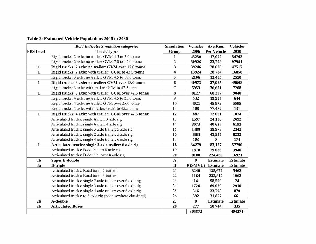
Table 2: Estimated Vehicle Populations 2006 to 2030

Bold Indicates Simulation categories Simulation Vehicles Ave Kms VehiclesPBS Level Truck Types Group 2006 Per Vehicle 2030

Rigid trucks: 2 axle: no trailer: GVM 4.5 to 7.0 tonne 1 45230 17,092 54762Rigid trucks: 2 axle: no trailer: GVM 7.0 to 12.0 tonne 2 80926 23,708 97981

1 Rigid trucks: 2 axle: no trailer: GVM over 12.0 tonne 3 39246 28,606 475171 Rigid trucks: 2 axle: with trailer: GCM to 42.5 tonne 4 13924 28,784 16858

Rigid trucks: 3 axle: no trailer: GVM 4.5 to 18.0 tonne 5 2106 13,485 25501 Rigid trucks: 3 axle: no trailer: GVM over 18.0 tonne 6 40973 27,985 49608

Rigid trucks: 3 axle: with trailer: GCM to 42.5 tonne 7 5953 36,671 72081 Rigid trucks: 3 axle: with trailer: GCM over 42.5 tonne 8 8127 68,307 9840

Rigid trucks: 4 axle: no trailer: GVM 4.5 to 25.0 tonne 9 532 19,957 644Rigid trucks: 4 axle: no trailer: GVM over 25.0 tonne 10 4621 45,973 5595Rigid trucks: 4 axle: with trailer: GCM to 42.5 tonne 11 108 77,477 131

1 Rigid trucks: 4 axle: with trailer: GCM over 42.5 tonne 12 887 72,061 1074Articulated trucks: single trailer: 3 axle rig 13 1597 24,108 2692Articulated trucks: single trailer: 4 axle rig 14 3673 40,627 6192Articulated trucks: single 3 axle trailer: 5 axle rig 15 1389 39,977 2342Articulated trucks: single 2 axle trailer: 5 axle rig 16 4883 45,937 8232Articulated trucks: single 4 axle trailer: 6 axle rig 17 103 0 174

1 Articulated trucks: single 3 axle trailer: 6 axle rig 18 34279 83,177 57790Articulated trucks: B-double: to 8 axle rig 19 1878 79,086 3940Articulated trucks: B-double: over 8 axle rig 20 8108 224,439 16921

2b Super B-double A 0 Estimate Estimate3a B-triple B 0 (SMVU) Estimate Estimate

Articulated trucks: Road train: 2 trailers 21 3240 135,679 5462Articulated trucks: Road train: 3 trailers 22 1164 232,819 1962Articulated trucks: single 2 axle trailer: over 6 axle rig 23 14 98,500 24Articulated trucks: single 3 axle trailer: over 6 axle rig 24 1726 69,079 2910Articulated trucks: single 4 axle trailer: over 6 axle rig 25 516 33,798 870Articulated trucks: to 6 axle rig (not elsewhere classified) 26 392 31,857 661

2b A-double 27 0 Estimate Estimate2b Articulated Buses 28 277 50,744 335

305872 404274

5

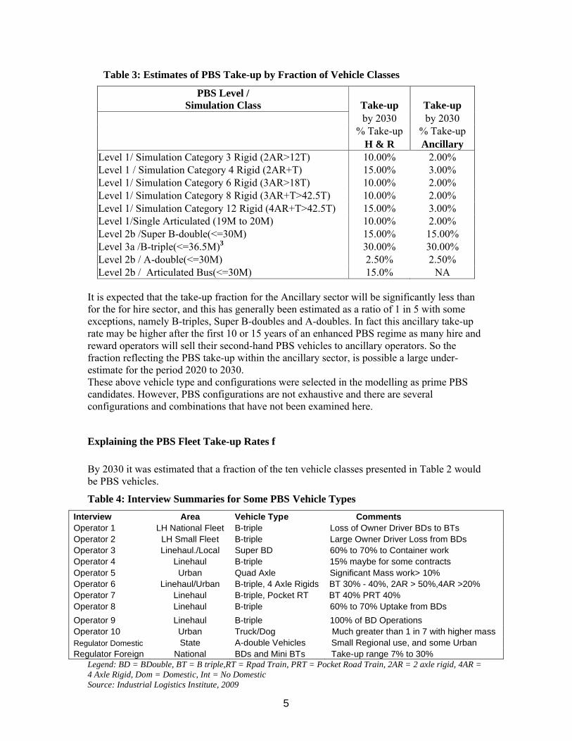
Table 3: Estimates of PBS Take-up by Fraction of Vehicle Classes

PBS Level / Simulation Class Take-up Take-up

by 2030 by 2030% Take-up % Take-up

H & R AncillaryLevel 1/ Simulation Category 3 Rigid (2AR>12T) 10.00% 2.00%Level 1 / Simulation Category 4 Rigid (2AR+T) 15.00% 3.00%Level 1/ Simulation Category 6 Rigid (3AR>18T) 10.00% 2.00%Level 1/ Simulation Category 8 Rigid (3AR+T>42.5T) 10.00% 2.00%Level 1/ Simulation Category 12 Rigid (4AR+T>42.5T) 15.00% 3.00%Level 1/Single Articulated (19M to 20M) 10.00% 2.00%Level 2b /Super B-double(<=30M) 15.00% 15.00%Level 3a /B-triple(<=36.5M)3 30.00% 30.00%Level 2b / A-double(<=30M) 2.50% 2.50%Level 2b / Articulated Bus(<=30M) 15.0% NA

It is expected that the take-up fraction for the Ancillary sector will be significantly less than for the for hire sector, and this has generally been estimated as a ratio of 1 in 5 with some exceptions, namely B-triples, Super B-doubles and A-doubles. In fact this ancillary take-up rate may be higher after the first 10 or 15 years of an enhanced PBS regime as many hire and reward operators will sell their second-hand PBS vehicles to ancillary operators. So the fraction reflecting the PBS take-up within the ancillary sector, is possible a large under-estimate for the period 2020 to 2030.These above vehicle type and configurations were selected in the modelling as prime PBS candidates. However, PBS configurations are not exhaustive and there are several configurations and combinations that have not been examined here.

Explaining the PBS Fleet Take-up Rates f

By 2030 it was estimated that a fraction of the ten vehicle classes presented in Table 2 wouldbe PBS vehicles.

Table 4: Interview Summaries for Some PBS Vehicle Types

Interview Area Vehicle Type CommentsOperator 1 LH National Fleet B-triple Loss of Owner Driver BDs to BTsOperator 2 LH Small Fleet B-triple Large Owner Driver Loss from BDsOperator 3 Linehaul./Local Super BD 60% to 70% to Container workOperator 4 Linehaul B-triple 15% maybe for some contractsOperator 5 Urban Quad Axle Significant Mass work> 10%Operator 6 Linehaul/Urban B-triple, 4 Axle Rigids BT 30% - 40%, 2AR > 50%,4AR >20%Operator 7 Linehaul B-triple, Pocket RT BT 40% PRT 40%Operator 8 Linehaul B-triple 60% to 70% Uptake from BDs

Operator 9 Linehaul B-triple 100% of BD OperationsOperator 10 Urban Truck/Dog Much greater than 1 in 7 with higher massRegulator Domestic State A-double Vehicles Small Regional use, and some UrbanRegulator Foreign National BDs and Mini BTs Take-up range 7% to 30%

Legend: BD = BDouble, BT = B triple,RT = Rpad Train, PRT = Pocket Road Train, 2AR = 2 axle rigid, 4AR = 4 Axle Rigid, Dom = Domestic, Int = No Domestic Source: Industrial Logistics Institute, 2009

6

This would range between 2.5% of the existing B-double fleet becoming A-doubles, to 30% of the growth in B-double fleet becoming B-triples by 2030. These estimates were drawn from 11 operator phone or personal interviews conducted after the 1st July 2009, and drawing on a decade of consultation with industry which has generated several peer reviewed research papers prior this date.

2. PBS COMMODITY NETWORKED BASED SIMULATIONS – PRELIMINARY ANALYSIS

2.1 ` Undertaking the PBS Commodity Network Based

Over the period, from 2006 to 2009, some 15 PBS case studies were undertaken by simulating different truck types carrying different commodities across different types of operational networks. A limited number of these case studies were made available to the NTC at that time.

Table 5: Commodity Freight Classes that will take up PBS

Operational Commodity Potential for PBS Take-up

Petroleum Yes

Other Tanker / Chemicals YesQuarry / earth / mining Yes

Over Dimensional YesCar Carrier Yes

Volumetric parcels Yes

Steel YesGrain Yes

Building Materials YesLogging YesWaste Yes

Container/wharf YesAgricultural Other No

Taxi Trucks YesRefrigerated Operations YesGeneral Freight Other No

Concrete YesMini Skips YesFurniture Yes

Horse movements (long trailer) YesGeneral Retail No

Livestock YesNon Specialised Courier No

Security Collections MaybeSource: Raptour Systems 2006e

The case studies were a first stage in the examination of the impact of PBS vehicles operating on different commodity networks. Further simulations were undertaken for this study.

7

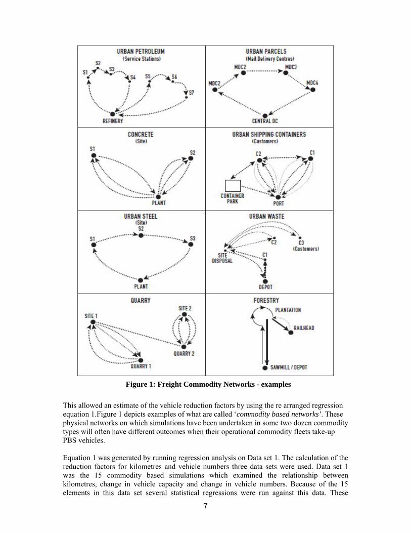
Figure 1: Freight Commodity Networks - examples

This allowed an estimate of the vehicle reduction factors by using the re arranged regression equation 1.Figure 1 depicts examples of what are called ‘commodity based networks’. These physical networks on which simulations have been undertaken in some two dozen commodity types will often have different outcomes when their operational commodity fleets take-up PBS vehicles.

Equation 1 was generated by running regression analysis on Data set 1. The calculation of the reduction factors for kilometres and vehicle numbers three data sets were used. Data set 1 was the 15 commodity based simulations which examined the relationship between kilometres, change in vehicle capacity and change in vehicle numbers. Because of the 15 elements in this data set several statistical regressions were run against this data. These

8

regressions yielded a simplistic business rule that was useful in the application for data set 2, and data set 3.

Table 6: Data Set 1 for the Calculation of Vehicle and Kilometre Reduction Factors

Source: University of Melbourne and Industrial Logistics Institute: Simulations 2006 to 2009

Equation 1

New Vehicle Factor = (New Kilometre Factor +(0.10 x Capacity Change) - 0.25) / 0.75

Table 7: Simulation Reduction factors for Longer Distance PBS Vehicles

Area/Simulation Commodity KM Factor Capacity Change Vehicles

Linehaul1 Inter Capital Parcels 0.7840 0.3300 0.700Linehaul2 Furniture 0.8000 0.3300 0.800Linehaul3 Livestock 0.7545 0.3300 0.800Regional1 Forestry 0.6250 0.3300 0.534Regional2 Mineral Sands 0.7600 0.3300 0.750

AverageLinehaul / Regional 0.7450 0.7167

Source: Industrial Logistics Institute Simulations

The averages from the simulation data output are presented in Table 7 and Table 8 for long distance and urban operations respectively. It should be noted that the massive impact of container related Super B-doubles, urban case 11, was excluded from the average of the other 10 urban case averages, however, the results were used for that specific vehicle type in the financial benefits estimation. Excluding urban case 11 reflects a conservative approach to the benefits estimation derived from the simulation approach. The kilometre and vehicle reduction factors represent that level that kilometres and vehicle numbers will reduce through the introduction of PBS vehicles into a freight transport operation.

Operation Commodity

KilometreReduction

FactorCapacity Change

Vehicle Reduction

FactorLinehaul Inter Capital Parcels 0.7840 0.3300 0.700Linehaul Furniture 0.8000 0.3300 0.800Linehaul Livestock 0.7545 0.3300 0.800Regional Forestry 0.6250 0.3300 0.534Regional Mineral Sands 0.7600 0.3300 0.750Urban Concrete 0.5590 1.0000 0.620Urban Urban Parcels 0.7390 0.4286 0.640Urban Intra Container Port 0.7490 1.0000 0.750Urban Outside Container Port 0.7500 0.3300 0.750Urban Steel Urban 0.8040 0.4800 0.670Urban General Parcels 0.8490 0.4280 0.778Urban Urban Mixed Fleets 0.8500 0.1590 0.889Urban Urban Tanker 0.9170 0.5100 0.875Urban Waste 0.8200 0.3300 0.720Urban Skips 0.7400 1.0000 0.750Urban Outside Container Port 0.5550 1.0000 0.556

9

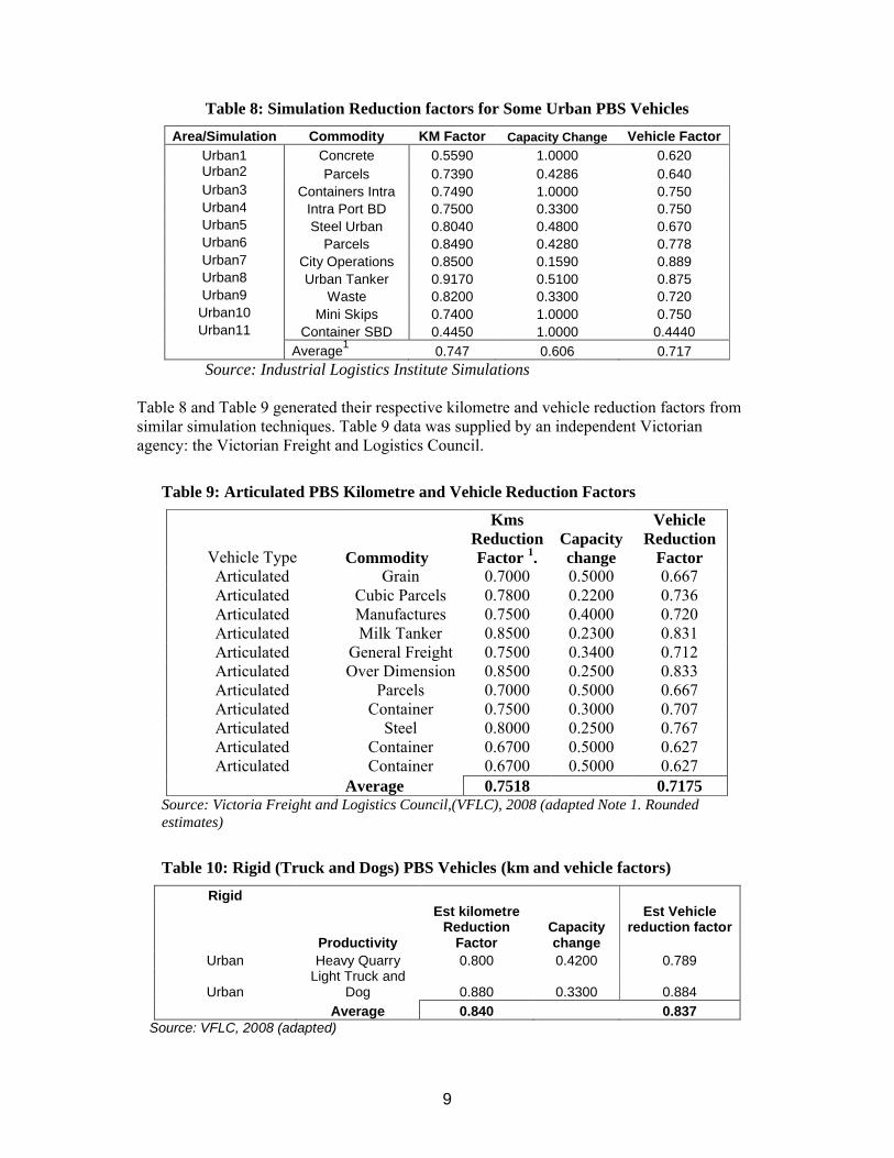
Table 8: Simulation Reduction factors for Some Urban PBS Vehicles

Area/Simulation Commodity KM Factor Capacity Change Vehicle Factor

Urban1 Concrete 0.5590 1.0000 0.620Urban2 Parcels 0.7390 0.4286 0.640Urban3 Containers Intra 0.7490 1.0000 0.750Urban4 Intra Port BD 0.7500 0.3300 0.750Urban5 Steel Urban 0.8040 0.4800 0.670Urban6 Parcels 0.8490 0.4280 0.778Urban7 City Operations 0.8500 0.1590 0.889Urban8 Urban Tanker 0.9170 0.5100 0.875Urban9 Waste 0.8200 0.3300 0.720

Urban10 Mini Skips 0.7400 1.0000 0.750Urban11 Container SBD 0.4450 1.0000 0.4440

Average1

0.747 0.606 0.717Source: Industrial Logistics Institute Simulations

Table 8 and Table 9 generated their respective kilometre and vehicle reduction factors from similar simulation techniques. Table 9 data was supplied by an independent Victorian agency: the Victorian Freight and Logistics Council.

Table 9: Articulated PBS Kilometre and Vehicle Reduction Factors

Vehicle Type Commodity

Kms Reduction Factor 1.

Capacity change

Vehicle Reduction

FactorArticulated Grain 0.7000 0.5000 0.667Articulated Cubic Parcels 0.7800 0.2200 0.736Articulated Manufactures 0.7500 0.4000 0.720Articulated Milk Tanker 0.8500 0.2300 0.831Articulated General Freight 0.7500 0.3400 0.712Articulated Over Dimension 0.8500 0.2500 0.833Articulated Parcels 0.7000 0.5000 0.667Articulated Container 0.7500 0.3000 0.707Articulated Steel 0.8000 0.2500 0.767Articulated Container 0.6700 0.5000 0.627Articulated Container 0.6700 0.5000 0.627

Average 0.7518 0.7175Source: Victoria Freight and Logistics Council,(VFLC), 2008 (adapted Note 1. Rounded estimates)

Table 10: Rigid (Truck and Dogs) PBS Vehicles (km and vehicle factors)

Rigid

Productivity

Est kilometre Reduction

FactorCapacity change

Est Vehicle reduction factor

Urban Heavy Quarry 0.800 0.4200 0.789

UrbanLight Truck and

Dog 0.880 0.3300 0.884

Average 0.840 0.837Source: VFLC, 2008 (adapted)

10

The Table 10 Data Set was derived from actual PBS applications for the Truck and Dog class of vehicles. (Rigid trucks with trailers). Vehicle reduction factors were derived from Equation 1.

Equation 2

New Total Kilometres = 0.75 x New Vehicles – (0.10 x Capacity Change) + 0.25

Equation 3

New Vehicles = (New Kilometres +(0.10 x Capacity Change) - 0.25) / 0.75

Equation 3 was again derived from the output of the urban commodity based simulations presented in Table 8.

Equation 4

New Urban Kilometres = 0.80 x New Urban Vehicles – (0.12 x Capacity Change) + 0.25

The savings for the longer distance operations, the urban operations and the truck and dog operations were used in the financial analysis. The exception being for the Super B-double which used simulation results across a 15% subset of the total urban articulated road transport task, which represented the container kilometre task for an example using the City of Melbourne, including vehicle operations being full, partly loaded or empty. It is certain that Super B doubles will also carry other commodities besides containers, so this was again a conservative assumption and should be revisited.

2.2 The Financial Benefits of PBS

The financial benefits of PBS were generated from applying the vehicle class take-up rate, divided by the total 20 year period, to estimate the number of PBS vehicles likely to emerge in that year. The PBS vehicle reduction factor is applied to a fraction of the vehicle population that will take up PBS. A reduction comes about as fewer PBS vehicles will be required to undertake a proportion of the task that would have been done by non PBS vehicles.The expected number of new PBS vehicles will also generate kilometre savings when the PBS kilometre factor is applied to the expected number of kilometres generated by that group of PBS vehicles. This reduction in kilometres is the basis for the benefits of PBS. The saved kilometres times the $/per kilometre rate for hire and reward and for ancillary operators is applied to their respective sectoral vehicle populations in each vehicle class for that year. It should be noted that generally ancillary operator costs are lower than the for hire operators as labour need not be fully paid against an award, eg a farmer, and generally trucks are older and therefore the operating cost profiles will also have a lower capital component.This process is repeated by vehicle class, each year, with the costs being escalated by the adjusted TransEco cost index.

The full PBS benefits by take-up vehicle type are presented in Table 12.

Equation 5

$ PBS Savings = ∑PBSv ∑n [(Kms saved)* ($/km Orig Veh Kms) – PBS Kms * (PBS $/km – Orig Veh $/km)]

The growth in vehicles – rigid, articulated, or B-double class, is applied to the next year’s vehicle population, and the process of new PBS vehicles is re-estimated, and the kilometresavings generated by these vehicles recalculated. This process is continued for the 11 vehicle classes that have been targeted for PBS take-up, over the 20 year period 2001 to 2030. The

11

vehicle operating costs are presented in Appendix B. The highest dollars per kilometre rates are not necessarily for the largest vehicles but can also be incurred by low, or very low,average kilometre vehicles.

The above equation suggests that there are kilometre savings in the original vehicle kilometres but this is offset somewhat by the extra cost of running PBS vehicles. This calculation is performed across each year from 2011 to 2030 and across all potential PBS vehicle types.

Table 11: Direct Operating Benefits of PBS Options, by Vehicle Class

PBS Vehicle type $ SavingsRigid trucks: 2 axle: no trailer: GVM over 12.0 tonne $270,028,079Rigid trucks: 2 axle: with trailer: GCM to 42.5 tonne $128,447,799Rigid trucks: 3 axle: no trailer: GVM over 18.0 tonne $421,102,673Rigid trucks: 3 axle: with trailer: GCM over 42.5 tonne $130,294,818Rigid trucks: 4 axle: with trailer: GCM over 42.5 tonne $24,139,103Articulated trucks: single 3 axle trailer: 6 axle rig $425,947,589Super B-double $704,711,545B-triple $3,060,210,825A-double $280,010,185Articulated Buses $7,881,125Total $5,452,773,742Industrial Logistics Institute estimates

3. PBS ‘FLOW-ON ECONOMIC EFFECTS’ – The INPUT-OUTPUT METHODS

3.1 Application of the Input-Output Method

The input-output system has found extensive use especially in economic forecasting and planning, both in the short and in the long run. It is especially useful in examining the impact of sub-sectors of the economy on the entire economy as a whole. In this case the use of I/O methods was used to estimate the flow on impacts of the savings generated by PBS to the rest

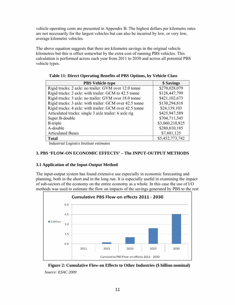
Figure 2: Cumulative Flow-on Effects to Other Industries ($ billion nominal)

Source: ESAC 2009

12

of the economy. The method has proved particularly effective in the analysis of sudden and large changes or other far-reaching transformations of an economy. In brief this extensive analysis was not included in the Benefit Cost Analysis but is outlined here as being an adjunct benefit which is not explored in this paper.This I/O method suggests that PBS also delivers a considerable benefit to the other non road transport sectors of the economy. Also the benefits from the analysis are certainly low as only the Hire and Reward flow-on benefits have been modelled.

CONCLUSION

Table 12 presents the impacts and savings in nominal terms for introducing PBS vehicles into Australia for the 20 year period 2011 to 2030.In brief the introduction of 13,848 vehicles will save some 4,362 existing type vehicles becoming operational. There will be a 3.7 billion kilometer saving . Total operational savings will approach 5.5 billion dollars with a further economic flow on of $4.5 billion in value added terms.

Table 12: Summary Benefits of Australian PBS for 2011 - 2030

PBS Metrics ImpactPBS Vehicles at 2030 13,848PBS Vehicle Savings at 2030 4,362PBS Vehicle Savings % of fleet at 2030 1.1%PBS Vehicle as % Fleet at 2030 3.5%PBS Kilometre Savings 2011 - 2030 3.7 Billion kmsPBS Kilometres at 2030 1.44 Billion kms% PBS Kilometres at 2030 6.60%Financial Savings ($) 2011 - 2030 $5.45BFlow on Impacts ($) 2011 - 2030 $4.57BTotal Operational and Financial Impacts $10.02B

Industrial Logistics Institute and ESAC Estimates

The estimation of this result was derived though the use of simulation tools looking at the impacts of seeding PBS vehicles onto commodity based networks. This is a new research area that warrants further investigation from both a freight efficiency and productivity perspective. The physical commodity networks provide a new template for PBS analysts to use nationally.

Appendix 1: Weighted Unit Costs per KilometreTable A1 reflects the weighted averages of vehicle costs in dollars per kilometre. The PBS and non PBS unit costs are a weighted average of for hire unit costs and ancillary unit costs. These two sectors are weighted by the population of vehicles in the class for each sector. In some instances the ancillary operator will have similar operating costs to the for hire operator but in most cases ancillary operating costs are lower than the for hire counterpart as labour is not costed at all against the transport operation, and capital equipment is based on the take up of a second hand vehicle.

Table A1: Unit Rates by Vehicle Class for PBS and non PBS VehiclesPBS Level / Simulation

Group Ave Kms PBS $/km1 Non PBS $/Km1

Level 1 / Cat 3 28,606 2.11 1.92Level 1 / Cat 4 28,784 2.21 2.01

13

Level 1 / Cat 6 27,985 2.68 2.44

Level 1 / Cat 8 68,307 3.15 2.86Level 1 / Cat 12 72,061 3.14 3.00

Level 1 / Single Articulated 83,177 1.55 1.54

Level 2b / Super B-double 35,000 3.21 2.69Level 3a / B-triple 224,439(e) 1.66 1.66

Level 2b / A-double 224,439(e) 1.76 1.76Level 2b / Articulated Bus 50,744 (e) 3.87 3.60

Source: 1. Translog unpublished databases(e) Estimated

Appendix 2: Vehicle Growth Rates and deflators to 2030The long term growth rates were calculated by examining the macro vehicle classes from 1971 to 2007 adjusted for rigid trucks below 4.5 tonnes and for non freight carrying articulated and rigid vehicles. The B-double growth rate calculated was not from their beginnings in 1986 which would yield a compound growth rate of 39% per annum, but instead from a stable level since 2004 when B-doubles have been at a steady level of 15.2% of SMVU articulated truck totals. This B-double percentage within the total articulated truck population was carried through till 2030. Many observers may argue that this B-double growth rate may be much higher but again this forecast was considered conservative, but it should be noted that any B-triple introduction will also cut into the existing growth in the B-double market.

Table A2: Annual Vehicle Growth Factors 2008 to 2030

B-double, A-double, B-triple growth rates p.a 1.032Single Articulated Trucks growth rates p.a 1.022

Rigid Trucks growth rates p.a 1.008

Road Transport Cost Escalators 1.0299NPV Discount Rate 1.07

Cost of Life escalator 1.03CO2 market escalator 1.07

Source: Industrial Logistics Institute 2009

REFERENCES and BIBLIOGRAPHY

1. Industrial Logistics Institute (2009) Forecasting the Benefits of Performance Based Standards for the Australian Road Transport Industry, 2011 to 2030, for the National Transport Commission, Melbourne, 1-82.

2. ABS, (2008), Australian Bureau of Statistics. ”Survey of Motor Vehicle Use, Category 9208.0”, Australian Bureau of Statistics, Canberra.

3. Victorian Freight and Logistics Council, (2008),“Higher Productivity Vehicle Industry Case”, HPV Case Study Examples”. HPV Taskforce, VFLC, Melbourne, Australia.

4. Hassall K, Thompson R, Larkins I. (2007), “Estimating the Benefits of Performance Based Standard vehicles in Australia”, 2nd T-Log Conference, Shenzhen China, Tsinghua University.

5. de Kievit, E.R, Aarts, L.(2007) ”Introduction of Longer Heavier Trucks on Dutch Roads”, Ministry of Transportation and Public Works, Transport Research Centre, the Netherlands.

6. Raptour Systems, (2006)“Impacts of Performance Based Standards in Australian Road Based Networks. Selected Case Studies”, Raptour Systems, Melbourne (for NTC).

14

7. Hassall K (2005), July, “Introducing High Product Vehicles into Australia: Two Case Studies”, Fourth International City Logistics Conference, pp 163 – 176, Proceedings IV City Logistics, Elsevier, ISBN 0 08 0447996

8. NRTC (1996),” Structure of the Australian Road Transport Industry”, NRTC, Melbourne.

9. TransEco (1994-2012),”TransEco Cost Indices”, Vol 1 to Vol 17, TransEco. Melbourne

GLOSSARY

BD B-doubleBT…B-tripleAD…A-doubleCO2 Carbon DioxideDFD Department of Finance and DeregulationESAC Economic and Statistical Analysis CanberraGVM…Gross Vehicle MassH&R…Hire and RewardILI Industrial Logistics InstituteI/O…Input-OutputNTC…National Transport CommissionNPV Nett Present ValueNTC…National Transport Commissionp.a. Per AnnumSBD Super B-doubleSMVU…Survey of Motor Vehicle UsePBS Performance Based StandardsL Linehaul OperationsR Regional OperationsU...Urban Operations2AR…2 Axle Rigid Truck3AR…3 Axle Rigid Truck4AR…4 Axle Rigid Truck 2AR + T…2 Axle Rigid Truck plus Trailer3AR + T…3 Axle Rigid Truck plus Trailer4AR + T…4 Axle Rigid Truck plus Trailer