The Puzzle of Muslim Advantage in Child Survival in India - Iza

IZA DP No. 4009

The Puzzle of Muslim Advantage in Child Survivalin India

Sonia BhalotraChristine ValenteArthur van Soest

DI

SC

US

SI

ON

PA

PE

R S

ER

IE

S

Forschungsinstitutzur Zukunft der ArbeitInstitute for the Studyof Labor

February 2009

The Puzzle of Muslim Advantage in

Child Survival in India

Sonia Bhalotra University of Bristol

and IZA

Christine Valente University of Nottingham

Arthur van Soest

Tilburg University and IZA

Discussion Paper No. 4009 February 2009

IZA

P.O. Box 7240 53072 Bonn

Germany

Phone: +49-228-3894-0 Fax: +49-228-3894-180

E-mail: [email protected]

Any opinions expressed here are those of the author(s) and not those of IZA. Research published in this series may include views on policy, but the institute itself takes no institutional policy positions. The Institute for the Study of Labor (IZA) in Bonn is a local and virtual international research center and a place of communication between science, politics and business. IZA is an independent nonprofit organization supported by Deutsche Post Foundation. The center is associated with the University of Bonn and offers a stimulating research environment through its international network, workshops and conferences, data service, project support, research visits and doctoral program. IZA engages in (i) original and internationally competitive research in all fields of labor economics, (ii) development of policy concepts, and (iii) dissemination of research results and concepts to the interested public. IZA Discussion Papers often represent preliminary work and are circulated to encourage discussion. Citation of such a paper should account for its provisional character. A revised version may be available directly from the author.

mailto:[email protected]

IZA Discussion Paper No. 4009 February 2009

ABSTRACT

The Puzzle of Muslim Advantage in Child Survival in India*

The socio-economic status of Indian Muslims is, on average, considerably lower than that of upper caste Hindus. Muslims have higher fertility and shorter birth spacing and are a minority group that, it has been argued, have poorer access to public goods. They nevertheless exhibit substantially higher child survival rates, and have done for decades. This paper documents and analyses this seeming puzzle. The religion gap in survival is much larger than the gender gap but, in contrast to the gender gap, it has not received much political or academic attention. A decomposition of the survival differential reveals that some compositional effects favour Muslims but that, overall, differences in characteristics between the communities and especially the Muslim deficit in parental education predict a Hindu advantage. Alternative outcomes and specifications support our finding of a Muslim fixed effect that favours survival. The results of this study contribute to a recent literature that debates the importance of socioeconomic status (SES) in determining health and survival. They augment a growing literature on the role of religion or culture as encapsulating important unobservable behaviours or endowments that influence health, indeed, enough to reverse the SES gradient that is commonly observed. JEL Classification: O12, I12, J15, J16, J18 Keywords: religion, caste, gender, child survival, anthropometrics, Hindu, Muslim, India Corresponding author: Sonia Bhalotra Department of Economics University of Bristol 8 Woodland Road Bristol BS8 1TN United Kingdom E-mail: [email protected]

* Sonia Bhalotra acknowledges funding from ESRC and DFID under research grant RES-167-25-0236 held at the CMPO in Bristol. Earlier versions of this paper were presented at a DFID and CMPO funded workshop on Child Health in Developing Countries in Bristol in June 2005 and at the European Society of Population Economics Conference in Verona in June 2006.

mailto:[email protected]

2

The Puzzle Of Muslim Advantage In Child Survival In India

Sonia Bhalotra, Christine Valente, Arthur van Soest

1. Introduction

Hindus and Muslim have cohabited in India for centuries, with Muslims ruling

most of the Indian subcontinent from the early 16th to the mid-19th centuries under the

Mughal Empire. However, today, their socioeconomic condition is thought to be not

much better than that of low caste Hindus, who have a long history of deprivation

(Government of India 2006).1 But despite being, on average, less educated and poorer,

Indian Muslims exhibit a substantial advantage in child survival. This paper documents

and analyses this seeming puzzle. It shows that the Muslim advantage is large, persistent,

and hard to explain.

A number of recent studies document socioeconomic status (SES) gradients in

health and survival, across countries, across SES groups within country and within

groups over time; for a survey see Cutler et al. (2006). Previous analyses of health

inequalities along ethnic or religious lines tend to start out with a differential consistent

with SES differences, as is the case, for example, with black-white differences in health

in the United States. While it has been recognised that unhealthy behaviours like smoking

or drinking may vary positively with SES (e.g. Rogers et al., 2000, p. 245), these are

seldom large enough to alter the raw differential in favour of the lower-SES group. The

case of Muslims in India is, in this respect, most unusual.

By age five, the Muslim survival advantage over Hindus is as high as 2.31%-

points, which is about 17% of baseline mortality risk amongst Hindus. Restricting the

comparison to upper-caste Hindus, who enjoy unambiguously higher social status than

Muslims, the differential is 1.30%-points, or about 10% of baseline mortality risk. Based

on the total number of births recorded in 2000 (Census of India 2001), and on the

proportions of high- and low-caste children born that year (obtained from representative

survey data used in this paper), this differential translates into an annual 127,955

(244,535) excess under-5 deaths amongst high-caste (low-caste) Hindus. To put the size

of this differential in perspective, consider that the more widely discussed gender

differential in under-5 mortality is 0.30%-points. Also, the average annual rate of

decrease in under-5 mortality risk between 1960 and 2001 in India was 0.61%-points p.a., 1 This is topical because the last two decades have witnessed renewed conflict between Hindus and Muslims (Varshney 2002), and this has also been a period of considerable political and socio-economic change.

3

which is about half the differential between Muslims and high-caste Hindus. The

Muslim-Hindu survival differential is not a new or an isolated phenomenon. It is evident

for most of the last half century. It has nevertheless claimed little public or academic

attention. Although it is flagged by Shariff (1995), Bhat and Zavier (2005), Bhalotra and

van Soest (2008) and Deolalikar (forthcoming), we know of no previous research that

carefully investigates this phenomenon.

This paper attempts to fill this gap, using microdata on more than 0.6 million

children born to about 200,000 Indian women during 1960-2006. The data and context

are described in Section 2. Section 3 profiles the seeming puzzle, showing how the

Muslim advantage varies by gender, age and birth order, how it has evolved over time,

and how it differs across Indian states and between rural and urban areas. Section 4

presents the estimation methods used. We use existing techniques for decomposition of

outcome differentials to investigate the extent to which the mortality differential can be

explained by the sorts of characteristics that are commonly used to explain or predict

child mortality rates (results are in Section 5). We then investigate alternative outcomes

and specifications (Section 6). Section 7 concludes. Our main finding is that the Muslim

advantage over high caste Hindus cannot be explained by the usual covariates included in

the model.

It is possible that there are omitted variables that improve survival and that are

inversely correlated with SES, but that have no particular relation to religion. The

layering of religion and caste in Indian society provides us with an opportunity to

investigate this. We do this by considering the extent to which the Muslim advantage

over low caste Hindus (of lower SES) is explained by the same set of characteristics. We

find that less than half of their advantage is explained. Overall, the evidence points to a

persistent Muslim “fixed effect” that favours child survival. The fixed effect survives our

attempts to include further controls for socio-economic status, access to health services

and rural infrastructure, maternal health and diet, and it is evident again when we

examine differences between Hindu and Muslim communities in child nutritional status.

Our findings suggest a research agenda that investigates what attitudes,

behaviours or unobserved traits Muslims might have, unlocking the key to which would

make an enormous impact on average mortality rates in India. We suggest that some of

the Muslim advantage may stem from their lower degree of son-preference, their closer

kinship, their more non-vegetarian diet, the better health of Muslim mothers and their

lower propensity to work outside the home.

4

The results contribute to a recent literature that argues that socioeconomic status

may not be as important a determinant of health or survival as attitudes at the individual

level and medical technology and services at the aggregate level (Cutler et al. 2006,

Fuchs 2004). It extends this discussion to incorporate the importance of culture or

community. Although there is a surge of interest amongst economists in ethnicity effects,

especially in education (e.g. Fryer and Levitt 2004, Wilson et al 2005), there remains

limited research on religion effects. The effects of religion on fertility have been

analysed, for example, for India (Bhat and Zavier 2005) and historical Europe (Guinnane

2005), but there is little work on religion and health. The analysis leads us to reconsider

the power of commonly estimated equations for mortality and health that neglect

unobserved heterogeneity between communities. The results also highlight the fact that

mortality is not systematically related to other indicators of health. In particular, although

the incidence of malnutrition by a cumulative indicator (height) is lower amongst

children in the higher SES group (Hindus), they are nevertheless more likely to die by the

age of five. This echoes the contrary patterns of malnutrition and mortality in

comparisons of sub-Saharan Africa and South Asia (e.g. Klasen 2003).

2. Background and Data

Muslims constituted 13.4% of the Indian population in 2001, up from 9.9% in

1951. Their total fertility rate was 3.06, as compared with 2.47 for Hindu women, a 24%

differential (Census of India 2001). The Sachar Committee Report commissioned by the

Indian Prime Minister documents their relatively weak social, economic and educational

status (Government of India 2006, henceforth GOI). Muslims are poorer than upper caste

Hindus, especially in urban areas (GOI). They have been less educated than upper caste

Hindus for decades and, although Muslim women have exhibited some catch-up, Muslim

men have not (Deolalikar forthcoming). There is intergenerational persistence in

education, which is a mechanism for the perpetuation of Muslim disadvantage (Bhalotra

et al. 2008). The educational deprivation of Muslims has been shown to drive their

disadvantage in the labour market (Bhaumik and Chakrabarty 2007). Their political

representation is small relative to their population share (GOI), and it has been argued

that the areas in which they are concentrated receive poorer public services (GOI).

Overall, the SES of Muslims is not much better than that of low caste Hindus. Yet,

although there are reserved places for the low castes in higher education, in public sector

jobs and in state legislatures, there is no similar positive discrimination in favour of

5

Muslims. These facts all make their relative success in averting child mortality quite

remarkable.2

To investigate the mortality differential, we stack three rounds of the National

Family Health Survey of India (NFHS) conducted in 1992/3, 1998/9, and 2005/06 (see

IIPS 1995, IIPS and ORC Macro 2000, and IIPS and Macro International 2007). These

surveys interviewed women aged 15-49 (13-49 in NFHS-1) at the time of the survey and

obtained complete fertility histories, including the dates of live births and of any child

deaths. The surveys contain information on relevant individual and household

characteristics, and the first two rounds also include information on village characteristics

including health infrastructure. Births in the original sample occur during 1954-2006. We

restrict the sample to mothers who are normal residents in the dwelling in which they are

interviewed. We drop children born before 1960 (0.08% of the sample), as the sample

sizes are very small for these years. We right-truncate the sample to ensure that all

children analysed have full exposure to the relevant mortality risk; for instance, for

under-5 mortality, we remove children less than 60 months old at the time of interview

(17.43% of births). We drop mothers who have ever had a multiple birth (3.11% of

births)3 and mothers for whom information on caste is missing (0.38% of all births). We

also drop the 11.49% of births in the survey that occur in households of religions other

than Muslim or Hindu, so that from now on, we refer to the mortality differential between

Muslim and Hindus as the religion-differential.4 The largest sample analysed (namely,

the one for children fully exposed to neonatal risk) has 653,496 live births of 197,952

mothers.

We pool data from across the states and include state fixed effects and trends in

the model. Our objective is to address the broad question of how Muslims and Hindus in

India as a whole compare although future work might focus on between-state differences.

Large samples are generated from the NFHS by using the full history of births. A

potential problem with this is recall bias in dates of birth and death, which is greater the

2 In this paper, low caste Hindus refers to scheduled castes and tribes (SC, ST). There are also castes within the Muslim community but they do not have the same history as the Hindu lower castes and castes not listed as SC or ST do not qualify for positive discrimination. 3 It is standard practice in the demographic literature to restrict the analysis to singletons as death risks are many times higher for multiple births and can skew the statistics. Amongst Muslims 1.48% of live births are multiple (twin, triplet etc) and amongst Hindus the corresponding figure is 1.29%. 4 Due to sampling design, the non-weighted share of births in households of religions other than Muslim or Hindu is much larger than the share of these other religions in the total population. When the number of births is corrected for sampling design, the share of the other religions is closer to figures from the population census: 4.2% of births compared to 6.1% of the population of all ages in 2001.

6

further back in time the event occurred. If any recall error is similar across communities

then this will not matter. We allow for recall that is expressed as age heaping by defining

indicators of mortality (e.g. under-5) to include deaths in the last month (e.g. 60th). A

second possible issue is that the further back one goes in time, the more scarce and the

less representative of the complete cohorts of children in these birth years is the sample

of births in the birth-history data because only mothers younger than 50 were

interviewed. This results in the early years including a disproportionate share of children

born to young mothers.5 These mothers are likely to be poorer and have higher fertility

than the average mother of children born at the same time. To account for this triangular

nature of the data structure, we condition on mother’s age at birth.

The heights and weights of children are indicators of the child’s nutritional status

(e.g. Micklewright and Ismail 2001). They were measured by surveyors for recent births

rather than reported by the mother. These data are therefore available for a shorter sample

of births that occurred 3-5 years before the survey. To render the samples in the three

rounds comparable, we restrict attention to the indicators of nutritional status of children

aged 0-3 and exclude the states of Andhra Pradesh, Madhya Pradesh, Tamil Nadu, West

Bengal, and Himachal Pradesh. The anthropometric data are standardized by age and

gender and reported as z-scores. They are, by their nature, subject to survival selection.

Sample weights included in the surveys are used to obtain summary statistics that

are representative for the all India population of mothers aged 15-49 at the time of the

survey and their children. Regressions are also weighted using these weights. The sample

we analyse changes because, for example, we drop births in the last month for the

analysis of neonatal mortality but we drop births in the last five years when we

investigate under-5 mortality. Alternatively, we are restricted to a shorter sample once we

incorporate a set of regressors that are only available for recent years. All descriptive

statistics are, unless otherwise stated, for the largest sample analysed, which is the sample

of children fully exposed to neonatal mortality risk in the pooled sample.

3. Descriptive Statistics

This section first describes the religion differential in mortality and the way in

which it varies with caste, age, gender, birth order, rural/urban and state location and 5 For example, in the 1998 round, births that occur near the survey date will come representatively from mothers aged 15 to 49. However, births in earlier years, for example 1968, come disproportionately from women who gave birth early. This is because older mothers, for instance age 25 in 1968, were 55 in 1998 and so excluded from the sample by design.

7

time. It also documents religion differentials in child nutritional status. It then describes

the explanatory variables used in the analysis.

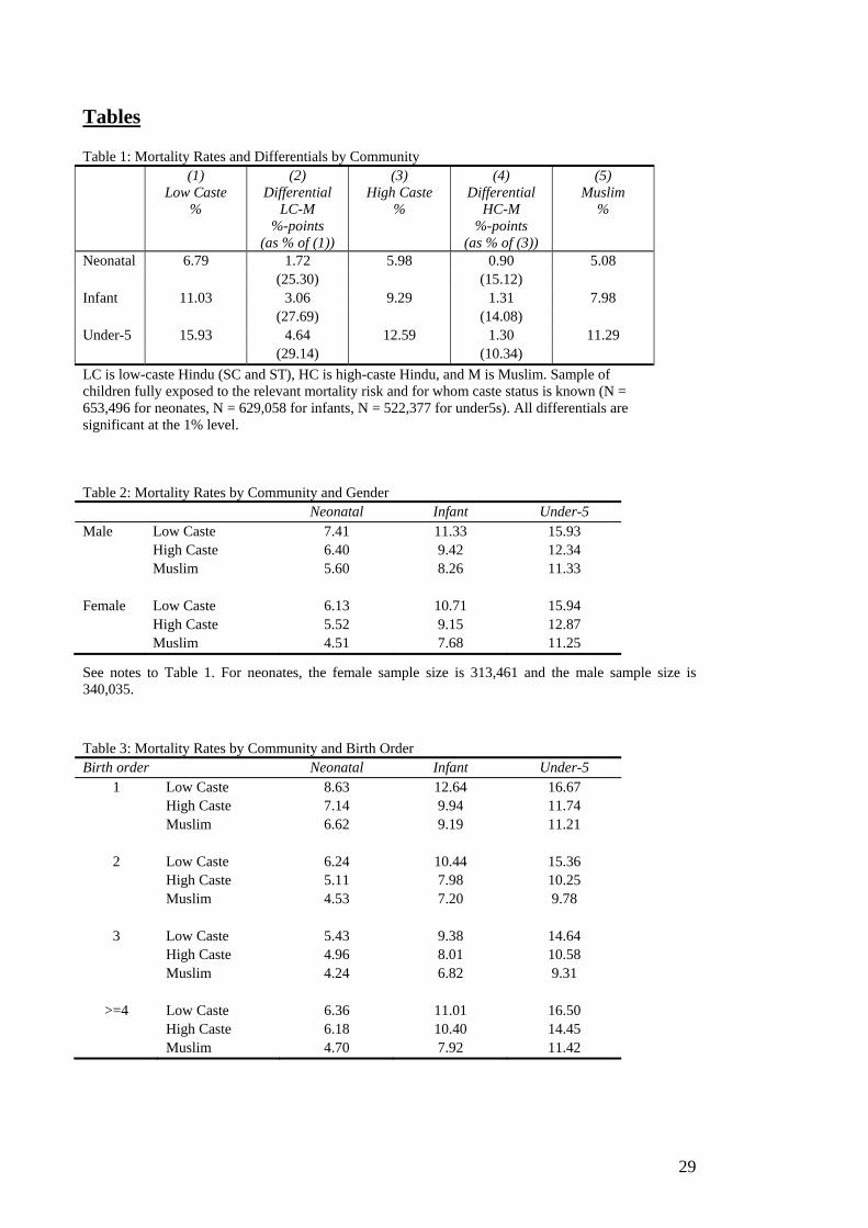
Table 1 goes about here.

Neonatal, infant, and under-5 mortality

Neonatal, infant and under-5 mortality are defined as the risk of dying between

birth and the age of one month, one year, and five years, respectively. After dropping

other religions, the sample of children analysed in this paper contains 84.58% Hindus and

14.42% Muslims. Across births in the data, which span the period 1960-2006, average

under-5 mortality is 15.93% amongst low caste Hindus, 12.59% amongst high caste

Hindus, and 11.29% amongst Muslims. So Muslims have an advantage of 2.31% points

(17% of baseline mortality risk) over all Hindus. Their advantage over low caste Hindus,

at 4.64%-points (29.14%) is, unsurprisingly, greater than their advantage over high caste

Hindus, which is 1.30%-points (10.34%). The latter is the real puzzle since upper caste

Hindus are clearly better off than Muslims, whereas lower caste Hindus are, by many

indicators, worse off (Government of India 2006). For neonatal [infant] mortality, the

raw differential relative to low caste Hindus is 1.72 [3.06] %-points, and relative to high

caste Hindus it is 0.90 [1.31] %-points.

In proportional terms, the mortality advantage with respect to high caste Hindus is

decreasing with age of exposure (Table 1). As much as 70% of the difference between

Muslims and high caste Hindus is established at birth, and the difference remains

constant from infancy up until age five. In contrast, the Muslim advantage with respect to

low caste Hindus is increasing in age of exposure, consistent with the higher SES of

Muslims as compared with the lower castes.


Averaging across communities, the under-5 survival advantage of boys over girls

is 0.30%-points. Disaggregating by community, we find that the all-India advantage of

boys over girls is entirely driven by high caste Hindus amongst whom the differential is

0.53%-points (Table 2). At birth, girls are, by nature, endowed with lower mortality risks.

Their advantage is eroded with age. It is notable that while the Muslim advantage over

low caste Hindus increases with age for both males and females, the Muslim advantage

over high caste Hindus only increases with age for females. By age five, there is no

gender difference in mortality rates amongst low caste Hindus, and girls exhibit an

advantage of 0.08%-points amongst Muslims. In Section 5.1 we shall see that these

8

patterns persist after conditioning on other covariates. These facts are striking, and

consistent with previous studies suggesting that higher caste Hindus exhibit greater son

preference than lower caste Hindus (e.g. Drèze and Sen 1997). The survival data analysed

here indicate that son preference amongst Muslims is lower than amongst Hindus and

especially high caste Hindus. The Muslim advantage over upper caste Hindus is greater

for girl survival, even if Muslims also show an advantage in boy survival. A lower degree

of son preference amongst Muslims would not only influence survival chances for

children of both genders by improving maternal health but it may further contribute to

reducing the gender gap in survival. A lower degree of son-preference amongst Muslims

(as compared with Hindus) is also apparent for other outcomes. For instance, Muslims

exhibit a lower sex ratio (males/females) at birth (e.g. Barooah and Iyer 2006) and a

smaller gender gap in educational enrolment (e.g. Bhalotra and Zamora forthcoming).


The Muslim/high caste differential increases monotonically with birth-order,

whereas the Muslim/low caste differential is nonlinear in birth order (Table 3). For

neonatal mortality, however, after conditioning on covariates including maternal age at

birth, it is only in the high caste group that the higher birth order child is significantly

more vulnerable (Section 5.1). These patterns are consistent with Muslims having a

higher taste for fertility.

Figure 1 goes about here.

The Muslim advantage is not a recent phenomenon, nor a diminishing one: see

Figure 1, and also see Bhat and Zavier (2005).6 Annual averages of religion-specific

mortality rates in survey data are subject to considerable sampling variation but taking

decadal averages, we find a Muslim under-5 survival advantage of 1.91%-points (8.9% of

the Hindu under-5 mortality rate) for births occurring during 1960-70 which decreased in

absolute but not in proportional terms to 1.64%-pts (16.24%) in 1990-2001.


Although the Muslim advantage over low caste Hindus is observed in both rural

and urban sectors, disaggregation by sector reveals that Muslims only do significantly

6 Their Table 6, p.389 reports the relevant means from the National Sample Surveys of 1963/4 and 1965/6, the Sample Registration Survey of 1979, Census 1981 and 1991, and the National Family Health Surveys (NFHS) of 1992/3 and 1998/9. In this paper, we use the NFHS surveys for 1992/3, 1998/9, and 2005/6, which contain information on births and child deaths over a span of 42 years. While data on mortality from surveys such as the NFHS can be subject to large sampling errors, SRS and Census data are not likely to suffer from this problem. The religion difference investigated here is apparent in these alternative data sets.

9

better than upper caste Hindus in rural areas (Table 4). For this reason, we investigate the

community differential for all-India as well as for the rural sample only. The Muslim

advantage is not driven by special circumstances in any one region; it is apparent in 11 of

26 states for high caste Hindus and in 19 of 26 states for low caste Hindus (see Appendix

Table 2). It is notable given our observations regarding community differences in gender

preference that the Muslim advantage is least visible in the East and the Northeast, where

Hindus have more matriarchal societies. Mortality rates vary substantially across the

states, as does the size and the religion-composition of the state population. States with a

higher proportion of Muslims appear to have lower under-5 mortality, although this may

simply be a composition effect, with the lower mortality risks of Muslims driving the

state average (Appendix Figure 1). States with a higher share of the country’s Muslim

population tend to have higher child mortality (Appendix Figure 2). The analysis to

follow allows for compositional effects by including state fixed effects and trends.

Nutritional Status

We investigate two indicators of nutritional status for children aged 0-3, namely

stunting and wasting. The first refers to height-for-age and indicates retardation of long-

term growth, and the second refers to weight-for-height, which reflects contemporaneous

insults to health (e.g. Martorell and Habicht 1986). Following WHO conventions, both

indicators are defined as equal to one if the child is more than two standard deviations

below the NCHS reference population median.7


The average child’s height-for-age and weight-for-height is below the reference

population median in every community. Long-term health outcomes are particularly

poor: the average low caste Hindu child is stunted, the average Muslim child is almost so,

and even the average high caste Hindu child is 1.8 standard deviations below the

reference median. Stunting rates are 52.0%, 46.7%, and 43.9% respectively. Indian

children fare better in terms of short-term health, with wasting rates at 20.3%, 17.3% and

16.9% (Table 5). The ranking of communities by stunting is consistent with their SES

ranking; this is less clear for wasting.8 While Muslim children are more often stunted

7 The U.S. National Center for Health Statistics (NCHS) standard, recommended by the World Health Organization (WHO) until recently, is the standard used to produce the z-scores provided in the first two NFHS waves. 8 Regressions of disease probabilities on parental education and indicators for caste and religion suggest that Muslim children are significantly more prone to fever and, in urban areas, also more prone to diarrhoea

10

than high caste Hindus, they are not more often wasted. Disaggregation by gender reveals

no boy-girl differences amongst Muslims and low caste Hindus. However, amongst high

caste Hindu, girls are shorter than boys (Table 6). This is a further indication of son

preference being most marked in this relatively well-off group. Overall, Muslims have no

large advantage in nutritional status that might directly explain their advantage in

survival, although they do a bit better on wasting than the better off high caste Hindu

group. We will investigate formally whether their better performance in weight-for-

height poses a puzzle analogous to that concerning their better survival performance.


To summarise, variation in community differences in survival by age of exposure

suggests that they may be related to maternal health, and community differences in

survival by birth order and gender indicate that at least some of the high caste Hindu

disadvantage may stem from their stronger preference for sons and their weaker

preference for high fertility (birth-order). Community differences in nutritional status are

much smaller than community differences in survival. Muslims have no advantage with

respect to stunting (height) and only a small advantage with respect to wasting (weight).

The Independent Variables

These include gender, birth order (whether born second, third, or fourth or above),

birth month and birth year of the child, categories for the age of the mother at the birth of

the child, rural/urban location of the household, a set of variables indicating the

educational level of the mother and of the father, state dummies, and state-specific trends.

This sort of specification is commonly used as a reduced form for the production of

health outcomes; see Strauss and Thomas (1995), for example. Education may be thought

to behave like technology in facilitating efficient use of inputs (Grossman 1972). It also

represents socioeconomic status.

All-India means by religion are in Appendix Table 1. Some relevant community

differences are summarised here. The sex ratio (male/female) at birth is lowest amongst

Muslims, and this difference is marginally statistically significant in relation to high caste

Hindus. As a consequence of higher Muslim fertility, a much larger share of Muslim

children are of fourth or higher birth-order. High caste Hindu mothers and fathers tend to

be more educated and the religion gap in education widens (in relative terms) with the (in the two weeks before the survey) than are Hindu children; see Bhalotra (2007), from whom detailed results are available upon request.

11

level of education. Averaging over the sample, Muslims are more educated than low

caste Hindus. Muslims are more urbanised than (all) Hindus and, although not shown in

these descriptive statistics, their poverty rate relative to Hindus is higher within urban

areas than within rural areas (GOI, p. 153). In this way, inequality in SES between

Muslims and Hindus appears to be lower in rural areas. The higher fertility of Muslims

has the consequence that the average child is of higher birth order but it also exerts

compositional effects associated with Muslim children being born, on average, to older

mothers and later in (calendar) time (Figure 2). Overall, it seems clear that the standard

(and especially, socioeconomic) predictors of mortality risk do not favour Muslims even

if some compositional effects may favour them.

Figure 2 goes about here.

4. Methods

We estimate community specific reduced-form logits for mortality of the form

(1) Mist* =F( xist, states, yeart, state*yearst; θ) + uist ;

Mist=1 if Mist*>0 and Mist=0 if Mist

*<0

Mist denotes an indicator variable with value 1 if child i born in year t and state s

dies before the reference age and 0 otherwise. The reference age varies, being either one

month (neonatal mortality), 12 months (infant mortality), or five years (under-5

mortality). States denotes a set of state dummies, yeart a set of child birth cohort

dummies, and state*yearst a set of interaction terms between state dummies and a linear

time trend that will control for state-time varying unobserved factors. The u term denotes

errors, assumed to be logistic, independent of the covariates, and independent for children

in different villages (but not necessarily for children of the same village), and θ is a

vector of parameters to be estimated. The vector xist contains exogenous or predetermined

child and household characteristics described in Section 3.9

Equation (1) is estimated separately for each of the three communities – low caste

Hindus, high caste Hindus and Muslims. (see Section 5.1). The Hindu-Muslim gap is

then decomposed to isolate the share due to differences in the independent variables

9 These include maternal age at birth and birth order which are endogenous if fertility is endogenous. Bhalotra and van Soest (2008) describe a structural model that endogenises them and estimate it for neonatal mortality. Their model does not hold for infant or under-5 mortality, and it is not a priority to model structural effects of birth-spacing or fertility on mortality because we observe lower death risks amongst Muslim children despite their higher fertility and shorter birth-intervals. We nevertheless estimated their structural model for the case of neonatal mortality, and found qualitatively similar results to those presented here.

12

across communities. This is done separately for low- and high caste Hindus (Section 5.2).

We then explore extensions to the set of regressors in the mortality model and also

investigate nutritional status rather than mortality (Section 6).

The decomposition uses an extension of the Blinder-Oaxaca technique that is

appropriate for binary models (Fairlie 2006, Jann 2006).10 The average difference in the

child mortality rate of the Hindu community H and the Muslim community M can be

expressed as:

( )( ) ( ) ( ) ( )

1 1 1 1

ˆ ˆ ˆ ˆ2

H M M MH H M H M H M MN N N Ni i i iH M

H M M Mi i i i

F X F X F X F XY Y

N N N N

θ θ θ θ

= = = =

⎡ ⎤ ⎡ ⎤⎢ ⎥ ⎢ ⎥− = − + −⎢ ⎥ ⎢ ⎥⎣ ⎦ ⎣ ⎦∑ ∑ ∑ ∑

with H indexing Hindus (either low- or high caste) and M indexing Muslims. JY (J=H,M) is the average probability of child death at the relevant age, JX is a row

vector of independent variables, ˆJθ is a vector of logit coefficient estimates including an

intercept and JN is the number of observations. The first term in Eq. (2), is the mortality

differential which we would see given the different characteristics of the two groups if

Muslims behaved like Hindus (i.e. with parameters set equal to ˆHθ for both groups). It is

an estimate of the extent to which the gap would close if Hindus were assigned the

characteristics of Muslims. We could just as well estimate this term forcing the responses

of the two groups to be represented by the parameters of the Muslim equation, ˆMθ . We

present both estimates.

The second term in equation (2) picks up the residual or “unexplained” variation

in mortality between the two groups. This may be interpreted as reflecting group-specific

cultural norms, information, discount rates, attitudes or indeed any omitted variables.

The characteristics effect can be further decomposed into contributions of (groups

of) covariates. For this purpose, it is necessary to match observations from both groups to

obtain samples of similar sizes. Since decomposition results are potentially sensitive to

the matching procedure, 100 low- or high caste Hindu samples were drawn randomly to

be matched with the (smaller) Muslim sample, and the reported results are means across

simulations. Moreover, when looking at the contribution of each variable, the order of

regressors in the equation matters since the contribution of each characteristic is

calculated conditional on the contribution of the previous ones (see Fairlie 2006, p.4).

10 Despite the popularity of the Blinder-Oaxaca approach, there are few instances of decomposition exercises for non-linear models; exceptions include Fairlie (2006) and Bauer et al. (2007).

13

This potential arbitrariness is minimised by randomising the ordering of the independent

variables in each replication and reporting the average results thus obtained. The detailed

decomposition is not sensitive to the choice of the omitted category for dummies

included in the model (Oaxaca and Ransom 1999).]

5. Results

5.1. Comparing determinants of child mortality amongst Muslims and Hindus

Logit estimates for under-5 mortality are in Appendix Table 5 and the

corresponding estimates for neonatal and infant mortality are in Appendix Table 4.

Consistent with the biological advantage of newborn girls, they have a significant

neonatal survival advantage in all three communities, and this is smallest amongst high

caste Hindus. By the age of five, the advantage of girls is eroded in every community

and, amongst high caste Hindus, it is turned around into a significant disadvantage.

Mortality odds tend to be highest for first-borns and then to increase with birth order

though less steeply for Muslims. It is notable that it is only for high caste Hindus that the

neonatal odds are significantly higher at birth-order four and higher. Note that the

estimated birth order effects are purged of the (correlated) effects of maternal age at birth

since this is also included in the equation. These findings tie in with long-standing

evidence of greater son-preference and lower desired fertility amongst high caste Hindus.

Mortality risk decreases monotonically with mother’s age at birth for low caste

Hindus and Muslims, except for Muslim infants of older (age 31-49) mothers, whose

mortality risk is higher than in the 25-30 category. Amongst high caste Hindus, mortality

odds decrease until age 25-30, before going up for older mothers. There is a tendency for

children born in March and October/November, when temperatures are, on average,

moderate, to face better survival chances. These effects are most clear in the low caste

group, possibly indicating that vulnerability to the epidemiological environment is

positively associated with poverty. The beneficial effects of parents’ education increase

with child age, consistent with an increasing role for environment and care in the survival

technology. In general, the effects of paternal and maternal education are similar across

the communities. As is commonly found, the coefficients on mother’s education are

somewhat larger than on fathers’ education, possibly because mothers are the principal

care-givers.

The disadvantage associated with living in a rural area is similar across

communities although it is a bit smaller amongst high caste Hindus. State of residence

14

matters more for Hindus than for Muslims. The year dummy coefficients, which are

jointly significant in all regressions, suggest that low caste Hindus have experienced the

smallest improvement in survival over time, and Muslims the largest. State-specific linear

trends are jointly significant for the two Hindu groups at any reference age, but they are

only significant for under-5 mortality amongst Muslims. Overall, there is significant

between-community variation in state-level unobservables and in the rate of decline of

mortality.

5.2. Baseline Decomposition Results

In this section, we present a decomposition of the mortality differential between

Muslims and high caste Hindus and between Muslims and low caste Hindus for each

mortality indicator. Estimates for under-5 mortality are in Tables 7 (whole sample) and 8

(rural sample). Estimates for neonatal and infant mortality are in Appendix Tables 6 and

7 respectively. The discussion will mostly focus on under-5 mortality where the paradox

is most pronounced, but the essential conclusions are similar for neonatal and infant

mortality. Results are benchmarked first on one parameter set ( ˆHθ ) and then on the other

( ˆMθ ). The results are sensitive to the choice of benchmark, but the overall conclusions of

the analysis are not.


Muslims versus High Caste Hindus

Differences in average characteristics between the communities predict a Muslim

disadvantage relative to high caste Hindus of 0.36%-points, explaining none of the 1.30%

points advantage that Muslims exhibit. The characteristics that drive the predicted

advantage of Hindus are their better parental education and their lower fertility, expressed

as lower average birth order. The decomposition reveals that Muslims gain some

advantage over Hindus on account of compositional factors. These are their greater

urbanisation and two compositional factors associated with their higher fertility. First, the

average Muslim child is born later in calendar time, which means it benefits from secular

improvements in medical technology and institutional quality, and second, Muslim

mothers are, on average, older at birth.11 State-specific trends also show some favour for

11 These results are for the case where high caste Hindus are the reference group. Alternative results are in the Tables.

15

Muslims. It is interesting that the higher fertility of Muslims exerts both direct and

compositional effects on their relative chances, the first negative and the latter positive.

Overall, the decomposition shows that compositional advantages that accrue to

Muslims on account of their location or their higher fertility are overwhelmed by their

lower levels of education. This confirms that the substantial survival advantage that they

exhibit remains, with the current (conventional) specification, a puzzle.

Muslims versus Low Caste Hindus

So as to detach omitted variables correlated with SES from religion and gain at

least a casual understanding of the role of SES versus religion (i.e. unobservables

associated with religion), we also compare Muslims with low caste Hindus. As discussed

earlier, high caste Hindus are distinctly better off than Muslims but Muslims are, by

many indicators, better off than low caste Hindus (Government of India 2006). The

decomposition shows that only about a third of the Muslim advantage over low caste

Hindus can be explained by the more favourable characteristics of Muslims.12


Isolating the Rural Sample

Although the all-India decomposition showed that their greater urbanisation

confers an advantage upon Muslims, we observed earlier that the Muslim advantage over

high caste Hindus is only significant in the rural sample (Section 3). We therefore repeat

the decomposition isolating rural households. In general, characteristics again completely

fail to explain the Muslim advantage. The closest we get is that in the comparison with

high caste Hindus that uses ˆHθ rather than ˆMθ , birth-year, state effects and state trends are

able to explain 10.6% of the Muslim advantage (Table 8).

So the paradox apparent in the raw data persists in that the better-off group does

worse and Muslims appear to carry a favourable community fixed effect. In the next

section, we put this assertion to the test by exploring extensions of the model, adding

covariates that have been omitted so far to see if including them in the model diminishes

the unexplained share of the Muslim advantage.

12 In contrast, about 56% of the high caste Hindu advantage over low caste Hindus is explained by differences in the same covariates. Results are available upon request.

16

6. Extensions

This section extends the analysis of mortality differences by adding controls for

household wealth, state expenditure on health and development, indicators of health

infrastructure at the village level and measures of maternal diet and health. It then

investigates how well community differences in anthropometric indicators are explained

by the more standard covariates.

The Role of Wealth

So far we have controlled for socioeconomic status using paternal and maternal

education. These are likely to be strongly correlated with wealth but, if Muslims are

systematically wealthier than Hindus for a given educational level, for instance, because

they own more land, then we may not be picking up adequately the effect of wealth

differentials. Although there is strictly no role for income or wealth in a health production

function since, together with prices, these determine the level of inputs, income or wealth

often appear in reduced form models of health (Strauss and Thomas 1995). Wealth is

endogenous if omitted regressors such as ability and social connections influence both

wealth and mortality or if mortality, by influencing the number of children and thus their

costs, determines wealth. This is therefore not our preferred specification but we

investigate it in order to be certain of the role of SES.

The NFHS contain information on a range of assets owned by households at the

time of the survey- there are no retrospective data that record the evolution of household

wealth over time that can be matched to the sequence of births in the retrospective

mortality data. We therefore restrict the sample to children born no more than 10 years

before the survey. The equation is estimated for under-5 mortality risk and so the sample

is further restricted to remove children who have not had five years exposed to this risk.

We use the first principal component of a set of assets as an indicator of wealth and

include a set of dummies for the quartile of the wealth distribution that the individual

household falls into.

Low and high caste Hindus face lower odds of dying if they are in the third or

fourth quartiles of the wealth distribution, but there are no significant wealth effects for

Muslims. The extended decomposition shows that wealth makes no contribution to the

Muslim-Hindu mortality differential. And, overall, in this smaller, more recent sample,

the overall contribution of characteristics to explaining the Muslim advantage is even

more negative than in the full sample (Appendix Tables 8A and 8B).

17

State-level Macroeconomic Variables

The baseline decomposition showed that state-time varying characteristics and

(later) year of birth favour Muslim children, especially relative to low caste Hindus. It

seems plausible that these reflect secular improvements in survival associated with the

quality and spread of medical facilities, health awareness and overall prosperity. These

same factors possibly also explain the higher mortality risk associated with rural areas.

We investigate this for under-5 mortality by looking at the effects of (log) real per capita

state expenditure on health and development projects, controlling for (log) real state

income per capita and for rural and urban income inequality using Gini coefficients.13 We

add to equation (1), for under-5 mortality, a vector of these state-level macroeconomic

variables. These data are only available for the 15 larger Indian states, which account for

more than 95% of India’s population, but result in us removing about 15.5% of

observations because women in smaller states are over-sampled in the NFHS design. We

find that state expenditure and income are insignificant but that rural inequality increases

child mortality amongst Muslims and high caste Hindus. Together, the set of

macroeconomic variables make no significant contribution to explaining the mortality

differential (see Appendix Tables 9A and 9B).

Village-level Infrastructure

So changes in state-level expenditure and income do not explain much of the

religion mortality differential, although state fixed effects and trends do. One potential

explanation is that the state-level variables are too aggregative; we do not know how

expenditure is distributed across villages with different concentrations of Hindus and

Muslims. Another is that increases in expenditure do not translate into effective

improvement in services because of absenteeism, corruption or absent complementary

inputs. We therefore consider directly indicators of the availability of health facilities at

the village level.

This information was only collected for rural areas and only in the first two

rounds of the survey. Since the data in these two rounds turn out not to be strictly

13 The effects of these variables are identified because the model includes state specific trends rather than interactions of state and time dummies.

18

comparable,14 this extension uses only the rural sample from NFHS-2. As facilities are

recorded for the time of the survey, we keep children born no more than six years before

the interview. This makes it hard to analyse under-5 mortality and allow 5 years exposure

and so this analysis is conducted for neonatal and infant mortality (Appendix Tables 10A,

10B and 10C). Given the short time-span and some fairly small state-specific samples,

we drop the state-specific time trends but, otherwise, the estimated model is as in

equation (1), with added village regressors. In this sample, the Muslim survival

advantage over high caste Hindus is not significant. However, even equal survival

chances of these groups represent a “puzzle” because, as we will show below, differences

in the characteristics of the two groups predict a Muslim disadvantage of up to 0.77%-

points (column 7).

The added village variables are the log of the village population, indicators for an

all-weather road, a pharmacy, a mahilamandal (women’s council), an anganwadi

(community childcare centre), a primary health centre, a primary health sub-centre, a

hospital, and dispensary or clinic.15 In both the neonatal and infant mortality

specifications, the contributions of the village variables to explaining the differential are

insignificant even if some are large in magnitude. Using more aggregated variables that

are comparable in NFHS-1 and NFHS-2, and thus using both datasets, we similarly found

no systematic evidence of differential access to health services after controlling for

village size in Bhalotra, Valente and van Soest (forthcoming). We identified some factors

that deepen the puzzle, such as the fact that Hindu women achieve better antenatal care

and child immunization and some that help explain it, such as that Muslim mothers are

more likely to seek treatment for diarrhoea, which is an important cause of child death.

Potential reasons behind the failure of village infrastructure differences to explain any of

the observed community differences in survival are (i) reverse causality, since areas with

higher mortality may be specifically targeted by health authorities - e.g. Rosenzweig and

Wolpin 1986; (ii) that access to facilities is largely disconnected from simple presence,

for example, due to time-poverty (e.g. Bhalotra 2007) or staff absenteeism (e.g.

14 For example, some unexpected patterns appear when comparing these data, such as a seeming reduction in the percentage of villages with a hospital or a clinic between NFHS-1 and NFHS-2. 15 For neonatal mortality, these variables are only jointly significant in the Muslim regression. For infant mortality, the only individually significant variables are the presence of a mahilamandal, which is correlated with higher infant mortality amongst low caste Hindus, most likely due to reverse causality going from higher mortality to the establishment of this type of centre, and the availability of an anganwadi, which is correlated with lower mortality amongst Muslims.

19

Chaudhury et al. 2006) and (iii) that quality of health facilities is weak – (e.g. World

Bank 2004).

Maternal health and diet

As we have seen in Section 3, a large share of the survival advantage of Muslims

is apparent at birth. This suggests a role for maternal health in explaining the puzzle. In

Bhalotra et al. (forthcoming), we show that Muslim women in India are taller, have

higher Body Mass Index (BMI), and are more likely to have a non-vegetarian diet than

their Hindu counterparts. We also show that each of these factors is associated with

improved survival chances for children.

Information on maternal height, BMI and diet is not available in NFHS-1, and so

we focus here on the two latest NFHS rounds. Since maternal BMI and diet at the time of

the survey are only relevant to children born in the few years preceding the survey, we

restrict the sample to children born no more than six years before the interview. As in the

case of village infrastructure, we drop the state-specific time trends but, otherwise, the

estimated model is as in equation (1) for neonatal mortality, augmented with a dummy

for vegetarian diet, a dummy for low BMI (i.e., BMI<18.5), its interaction with an

indicator for being pregnant at the time of the interview, and the logarithm of maternal

height (see Appendix Tables 12A and 12B). In this sample, the advantage of Muslim

mothers in terms of height and BMI is only significant relative to low-caste Hindu

mothers. We find that a vegetarian diet has an adverse impact on neonatal mortality for

high-caste Hindus, and no significant impact in the other groups. Low BMI does not

significantly affect neonatal mortality unless extreme, as indicated by the statistically

significant effect of the interaction between the dummies for low maternal BMI and

pregnancy. Taller mothers in every community are significantly less likely to see their

children die in the first month of life (see Appendix Table 12A; Bhalotra and Rawlings

2008).

The decomposition of the community differential shows that maternal height

explains some of the Muslim advantage over low-caste Hindus and a non-vegetarian diet

explains some of their advantage over high-caste Hindus. Differences in BMI only

reinforce the puzzle of the Muslim advantage over high-caste Hindus. We also estimated

an alternative specification in which the only regressor added to our baseline model is

maternal height. The advantage of this is that, as maternal height is time-invariant, we

can now use the complete set of births as before. Pooling data from NFHS-2 and NFHS-

20

3, we find that Muslim mothers have a height advantage over high and low caste Hindus.

Analysing under-5 mortality, we find that this contributes to explaining some of the

Muslim advantage, but the overall message from the decomposition is again that

differences in characteristics add up to predict a high-caste Hindu advantage over

Muslims, leaving the observed advantage of Muslims unexplained (see Appendix Tables

13A and 13B).

To summarise, controlling for household wealth, access to health services and

public infrastructure, and maternal health and diet does not contribute much to

understanding the puzzle of why mortality among children of Muslims is lower than

among children of Hindus .

Nutritional Status

We noted in Section 3 that community differences in anthropometric deficits

present a more mixed picture than for survival rates. We expect that nutritional status is

correlated with survival although it is unclear whether it plays a causal role; see Almond

et al. (2005) who suggest that mother-level heterogeneity is likely to be a strong

confounder in the cross-sectional literature on birth weight. We cannot investigate this

with our data because anthropometrics are only measured for children alive at the time of

the survey. Indeed, there is survival selection in the data on heights and weights. To the

extent that it is children with low potential height and weight who succumb early to

mortality and are eliminated from the sample, we may expect greater similarity across

communities in anthropometrics than we do in mortality rates.

The sample for this part of the analysis was described in Section 2, and stunting

and wasting were defined and summarised in Section 3. The set of regressors is as in

equation (1) although we do not include state-specific trends because this sample is

relatively short, consisting of three years for each of the three survey rounds. The logit

estimates are in Appendix Table 11.

Consider stunting first, for which the ranking of communities is consistent with

their SES. The decomposition shows that between 75 and 94 per cent of the high caste

Hindu advantage over Muslims is on account of differences in characteristics (Table 9).


The characteristics that favour high caste Hindus are parental education, birth order and

month of birth, and their advantage is only partly offset by a Muslim advantage on

account of their urbanisation, birth year and state of residence. The Muslim advantage

21

over low caste Hindus is more enigmatic. No more than 29% of the differential in

stunting is explained by differences in characteristics. Mother’s education, age at birth

and birth year disadvantage lower caste Hindus and overwhelm factors that disadvantage

Muslims, namely, higher birth order, distribution of month of birth and father’s

education.16 Thus there appear to be omitted variables specific to Muslim children that

favour their height performance relative to low caste Hindus. When Muslims do worse,

as is the case compared with high caste Hindus, then most of their disadvantage is

explained. However, when they do better, as is the case relative to low caste Hindus, their

advantage is unexplained. This is consistent with our earlier finding that the Muslim

community has some unobservable traits that favour health.


Now consider wasting, the indicator on which Muslims do relatively well.

Although wasting amongst Muslims is lower by 0.40%-points, differences in

characteristics suggest it should be higher by up to 0.56%-points, compared with high

caste Hindus, who are favoured again by better parental education and lower birth order.

Muslims do better than the low caste group but at most 20% of their advantage is

explained by characteristics and this rests upon unobservables captured by the state

dummies (Table 10). So Muslims show an unexplained advantage relative to both castes

of Hindus in avoiding low weight-for-age just as they do in avoiding mortality. The

summary results are arrayed for our many alternative specifications in Table 11.Table 11

goes about here.

7. Conclusion

Our initial specification examined the contribution to the community survival

differential of parental education, family demographics and state and cohort-specific

unobservables for three indicators of survival and two indicators of nutritional status. For

survival, we further explored the contribution of asset ownership, state macroeconomic

variables, rural health services and infrastructure, and maternal health and diet. We find

that, in general, none of the Muslim advantage over high caste Hindus can be explained

while, typically, less than half of their advantage over low caste Hindus can be explained

by differences in characteristics.

16 In this short sample, Muslim fathers are less educated than low caste Hindus. This is a reflection of the more rapid educational progress of low caste as compared with Muslim men over time. In contrast, Muslim women have advanced fairly rapidly (see Deolalikar 2008).

22

The essence of the paradox that this paper highlights is that, when we consider

averages by religious community in India, then the commonly found positive association

of socioeconomic status and survival breaks down. Our decomposition of the community

differential suggests that the effects of SES are overwhelmed by some unobservable trait

owned by the lower SES group.17 Correlates of religion that may plausibly influence

survival without exhibiting a strong positive correlation with SES include diet, attitudes

to women’s work, personal hygiene, political clout or social norms and networks. Some

of these effects may be better cast as historical, cultural or biological factors in that they

are unrelated to religious belief per se even if they have gelled around a community that

is identified by its religion.

Some clues emerged from profiling the religion differential by age, gender and

birth order (Section 3). More than two-thirds of the survival advantage of Muslims over

high-caste Hindus is apparent at birth and, in proportional terms, it decreases between the

age of one and five. This suggests that explanations of the differential may have more to

do with maternal health, delivery and early feeding practices and less to do with access to

resources or public services post-infancy. If we argue that maternal health is key, then we

must also argue that there are aspects of maternal health that are not directly linked to

their SES, or else controlling for parental education and asset ownership would have

explained at least part of the differential.

Scattered evidence suggests that there are. For example, a lower degree of son

preference amongst Muslim as compared with Hindu households (see Section 3) may

have meant that Muslim mothers received a more equal share of household resources in

their own childhoods. This is suggested to hold in Basant (2007). Trends in adult height

for birth cohorts 1956-86 are also consistent with this assertion, given evidence that

childhood conditions have a profound influence on adult height (Bozzoli et al.

forthcoming): Over this period, Muslim women gained height significantly faster than

Hindu women, while Muslim men grew more slowly than Hindu men (Bhalotra 2008).

Alternatively, better maternal health amongst Muslims may be the result of their having a

more balanced or non-vegetarian diet (Section 6), or of their being less likely to work

during and just after pregnancy (Bhalotra et al. forthcoming). A third factor that may

favour maternal health amongst Muslims despite their lower SES is their stronger kinship

structures which, in part, have to do with a greater prevalence of endogamy in this 17 Read Muslims relative to high caste Hindus, although comparisons of Muslims with low caste Hindus reinforce this conclusion.

23

community. This is associated with lower marriage payments and the perception of the

girl child as less of a burden, as well as with the availability of extended care for the

mother and the newborn child from the natal family (e.g. Robinson 2007). It may also

make for better information sharing amongst women, and stronger insurance networks.

In Bhalotra et al. (forthcoming), we show that antenatal care practices are less

favourable to child survival amongst Muslims, and that Muslim women give birth outside

medical facilities more often than their Hindu counterparts, thus reinforcing the puzzle.

On the other hand, in the same study we find that Muslim women tend to put the baby to

the breast sooner after birth. This may contribute to explaining the Muslim survival

advantage. Differences in maternal BMI and vegetarian diet at the time of the survey, as

well as in maternal height, make only a small contribution to explaining the puzzle

(Section 6), but further research using alternative measures of mother’s health and

maternal and child diet, in particular during pregnancy and in the immediate postnatal

period (including breastfeeding), may shed more light on the conundrum.

Although there is no evidence on which way this goes, it is worth flagging a

potential role here for differences in foetal survival. Since the evidence points to the

importance of maternal health, it is plausible that Muslims not only have (visibly) better

survival chances of newborn children but that they experience, for the same reasons,

(invisibly) lower risks of foetal death. This would contribute to explaining the higher

fertility of Muslim women which, so far, has been explained in terms of higher desired

fertility and greater aversion to the use of contraception. However, selection may turn this

around. If poverty (SES) dominates in the risk of foetal loss and Muslims are in fact more

likely than upper caste Hindus to suffer it then, assuming that it is the frailest children

who die in utero; the average live birth amongst Muslims will tend to be less frail and

more likely to survive. This may contribute to explaining the higher survival chances of

Muslim children (which is, by convention, measured as a fraction of live births).

There is a clear agenda for future research in this area. Differences between

communities in maternal health and in attitudes to pregnancy may create differences in

foetal death risk, with consequences for observed differences in both childhood mortality

and fertility. This has not been previously investigated. It would be useful for policy if we

could separate inalienable characteristics from behaviours (like labour supply or

treatment of sons versus daughters) that are more transferable and, related, if we could

identify the extent to which information or risk-sharing networks operate along religion

lines (e.g. Munshi and Myaux (2006) find that social change emerges from separate

24

social interaction amongst Muslims and Hindus in rural Bangladesh). It would also be

useful to map the geographic distribution of low and high caste Hindus and Muslims at

the village level, to indicate, for example, the degree of residential segregation of the

communities. This may have implications for the provision of public services (Alesina et

al. 1999). Finally, it would be instructive to directly consider the political economy of

public provision and the extent to which it is influenced by caste and religion of both

elected leaders and constituency members (e.g. Pande 2003).

25

References

Alesina, Alberto, Reza Baqir and William Easterly (1999), “Public Goods and Ethnic

Divisions,” Quarterly Journal of Economics, November 1999, 114: 1243-84.

Almond, Douglas, Kenneth Chay and David Lee. 2005. "The Costs of Low Birth

Weight". Quarterly Journal of Economics 120(3): 1031-1083.

Barooah, Vani K. and Sriya Iyer. 2005. "Vidya, Veda and Varna: The Influence of

Religion and Caste on Education in Rural India". Journal of Development Studies 41(8):

1369-1404.

Bauer, Thomas, Silja Golhmann and Mathias Sinning. 2007. "Gender Differences in

Smoking Behavior". Health Economics 16:895-909.

Basant, Rakesh. 2007. "Social, Economic and Educational Conditions of Indian

Muslims". Economic and Political Weekly 42(10): 828-832.

Bhalotra, Sonia. 2007. "Fatal Fluctuations? Cyclicality in Infant Mortality in India, IZA

Discussion Paper 3086". Institute for the Study of Labor (IZA), Bonn.

Bhalotra, Sonia. 2008. "Gender Differentials Again: Evidence from Cohort Profiles of the

Heights of Men and Women". Mimeograph, University of Bristol.

Bhalotra, Sonia, Arnim Langer, Frances Stewart and Bernarda Zamora. 2008. "Persistent

Muslim/Hindu Inequalities in India". Mimeograph, CRISE, University of Oxford.

Bhalotra, Sonia and Sam Rawlings. 2008. "The Intergenerational Transmission of Health

in Developing Countries". Mimeograph, University of Bristol.

Bhalotra, Sonia, Christine Valente and Arthur van Soest. Forthcoming. "Religion and

Childhood Death in India" In Handbook of Muslims in India, ed. A Sharif and R Basant,

Delhi: Oxford University Press.

Bhalotra, Sonia and Arthur van Soest. 2008. "Birth-Spacing, Fertility and Neonatal

Mortality in India: Dynamics, Frailty, and Fecundity". Journal of Econometrics 143(2):

274-290.

Bhalotra, Sonia and Bernarda Zamora. Forthcoming. "Social Divisions in Education in

India" In Handbook of Muslims in India, ed. A. Sharif and R. Basant, Delhi: Oxford

University Press.

Bhat, Mari and Francis Zavier. 2005. "Role of Religion in Fertility Decline: The Case of

Indian Muslims". Economic and Political Weekly 40(5): 385-402.

26

Bhaumik, Sumon K. and Manisha Chakrabarty. 2006. "Earnings Inequality in India: Has

the Rise of Caste and Religion Based Politics in India Had an Impact?" Working Paper

819, William Davidson Institute, University of Michigan.

Bozzoli, C, Angus Deaton and C Quintana-Domeque. Forthcoming. "Adult Height and

Childhood Disease". Demography.

Census of India. 2001. "Fertility Tables, available online at

http://www.censusindia.gov.in/Data_Products/Data_Highlights/Data_Highlights_link/dat

a_highlights_F9_F10.pdf."

Chaudury, Nazmul, Jeffrey Hammer, Michael Kremer, Karthik Muralidharan and Halsey

Rogers. 2006. "Missing in Action: Teacher and Health Worker Absence in Developing

Countries". Journal of Economic Perspectives 20(1): 91-116.

Cutler, D, Angus Deaton and A Lleras-Muney. 2006. "The Determinants of Mortality".

Journal of Economic Perspectives 20(3): 97-120.

Deolalikar, Anil B. Forthcoming , How Do Indian Muslims Fare on Social Indicators? In

Handbook of Muslims in India, ed. A Sharif and R Basant, Delhi: Oxford University

Press.

Drèze, Jean and Amartya Sen. 1997. Indian Development: Selected Regional

Perspectives, Oxford: Clarendon Press.

Fairlie, Robert. 2006. "An Extension of the Blinder-Oaxaca Decomposition Technique to

Logit and Probit Models". IZA Discussion Paper No. 1917, Institute for the Study of

Labor (IZA), Bonn.

Fryer, R.G. and S.D Levitt. 2004. "Understanding the Black-White Test Score Gap in the

First Two Years of School". Review of Economics and Statistics 86: 447-464.

Fuchs, Victor R. 2004. "Reflections on the Socio-Economic Correlates of Health".

Journal of Health Economics 23: 653-661.

Government of India. 2006. "Social, Economic and Educational Status of the Muslim

Community of India: A Report. Prime Minister’s High Level Committee".

Grossman, Michael. 1972. The Demand for Health: A Theoretical and Empirical

Investigation. New York: Columbia University Press for the National Bureau of

Economic Research.

Guinnane, Timothy. 2005. "The Fertility Transition in Europe”. European Society of

Population Economics, keynote address.

IIPS. 1995. "National Family Health Survey (MCH and Family Planning), India 1992-

93." International Institute for Population Sciences (IIPS), Mumbai.

27

IIPS and ORC Macro. 2000. "National Family Health Survey (NFHS-2) 1998-99 India".

International Institute for Population Sciences (IIPS), Mumbai.

IIPS and Macro International. 2007. "National Family Health Survey (NFHS-3), India

2005-06". International Institute for Population Sciences (IIPS), Mumbai.

Jann, Ben. 2006. "Fairlie: Stata Module to Generate Nonlinear Decomposition of Binary

Outcome Differentials. Available from http://ideas.repec.org/c/boc/bocode/s456727.html.

Klasen, Stephan. 2003. "Malnourished and Surviving in South Asia, Better Nourished

and Dying Young in Africa: What Can Explain this Puzzle?" In Measurement and

Assessment of Food Deprivation and Undernutrition, ed. FAO, Rome: FAO.

Martorell, Reynaldo and Jean-Pierre Habicht. 1986. "Growth in Early Childhood in

Developing Countries" In Human Growth: A Comprehensive Treatise. Volume 3:

Methodology and Ecological, Genetic, and Nutritional Effects on Growth, 2nd ed., ed.

Frank Falkner and J.M. Tanner, New York: Plenum Press.

Micklewright, John and Suraiya Ismail. 2001. “What Can Child Anthropometrics Reveal

About Living Standards and Public Policy: An illustration from Central Asia”, Review of

Income and Wealth, March, Vol. 47 Issue 1, p 65-80.

Munshi, Kaivan and Jacques Myaux. 2006. “Social Norms and the Fertility Transition.”

Journal of Development Economics 80(1):1-38.

Oaxaca, Ronald and Michael Ransom. 1999. "Identification in Detailed Wage

Decompositions". The Review of Economics and Statistics 81(1): 154-157.

Pande, Rohini. 2003. “Can Mandated Political Representation Provide Disadvantaged

Minorities Policy Influence? Theory and Evidence from India”. American Economic

Review, Vol. 93(4), pp. 1132-1151, September.

Robinson, Rowena. 2007. "Indian Muslims: The Varied Dimensions of Marginality".

Economic and Political Weekly 42(10): 839-843.

Rogers, Richard G., Robert A. Hummer and Charles B. Nam. 2000. Living and Dying in

the USA. Behavioral, Health, and Social Differences in Adult Mortality. New York:

Academic Press.

Rosenzweig, Mark and Kenneth Wolpin. 1986. "Evaluating the Effects of Optimally

Distributed Public Programs: Child Health and Family Planning Interventions". American

Economic Review 76: 470-482.

Shariff, Abusaleh. 1995. "Socio-Economic and Demographic Differentials between

Hindus and Muslims in India". Economic and Political Weekly 30(46): 2947-2953.

28

Straus, John and Duncan Thomas. 1995. "Human Resources: Empirical Models of

Household Decisions" In Handbook of Development Economics, Volume IIIA, ed. J.R.

Behrman and T.N. Srinivasan, Amsterdam: North Holland.

Varshney, Ashutosh. 2002, Ethnic Conflict and Civic Life: Hindus and Muslims in India,

Yale University Press.

Wilson, Deborah, Simon Burgess and Adam Briggs. 2005. "The Dynamics of School

Attainment of England’s Ethnic Minorities". Working Paper 05/130, CMPO, University

of Bristol.

World Bank. 2004. World Bank Development Report: Making Services Work for Poor

People. World Bank, Washington DC.

29

Tables Table 1: Mortality Rates and Differentials by Community (1)

Low Caste %

(2) Differential

LC-M %-points

(as % of (1))

(3) High Caste

%

(4) Differential

HC-M %-points

(as % of (3))

(5) Muslim

%

Neonatal 6.79 1.72 5.98 0.90 5.08 (25.30) (15.12) Infant 11.03 3.06 9.29 1.31 7.98 (27.69) (14.08) Under-5 15.93 4.64 12.59 1.30 11.29 (29.14) (10.34) LC is low-caste Hindu (SC and ST), HC is high-caste Hindu, and M is Muslim. Sample of children fully exposed to the relevant mortality risk and for whom caste status is known (N = 653,496 for neonates, N = 629,058 for infants, N = 522,377 for under5s). All differentials are significant at the 1% level.

Table 2: Mortality Rates by Community and Gender Neonatal Infant Under-5 Male Low Caste 7.41 11.33 15.93 High Caste 6.40 9.42 12.34 Muslim 5.60 8.26 11.33 Female Low Caste 6.13 10.71 15.94 High Caste 5.52 9.15 12.87 Muslim 4.51 7.68 11.25

See notes to Table 1. For neonates, the female sample size is 313,461 and the male sample size is 340,035.

Table 3: Mortality Rates by Community and Birth Order Birth order Neonatal Infant Under-5

1 Low Caste 8.63 12.64 16.67 High Caste 7.14 9.94 11.74 Muslim 6.62 9.19 11.21



>=4 Low Caste 6.36 11.01 16.50 High Caste 6.18 10.40 14.45 Muslim 4.70 7.92 11.42

30

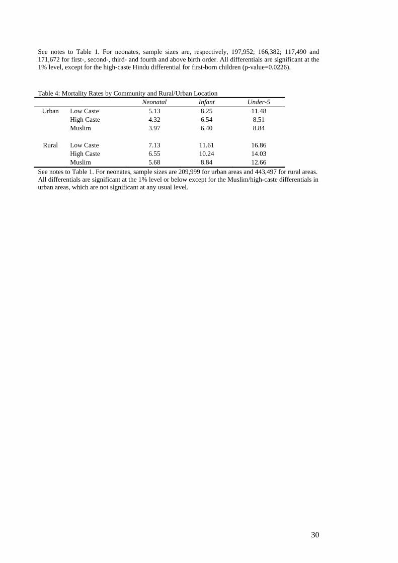
See notes to Table 1. For neonates, sample sizes are, respectively, 197,952; 166,382; 117,490 and 171,672 for first-, second-, third- and fourth and above birth order. All differentials are significant at the 1% level, except for the high-caste Hindu differential for first-born children (p-value=0.0226). Table 4: Mortality Rates by Community and Rural/Urban Location Neonatal Infant Under-5

Urban Low Caste 5.13 8.25 11.48 High Caste 4.32 6.54 8.51 Muslim 3.97 6.40 8.84

Rural Low Caste 7.13 11.61 16.86 High Caste 6.55 10.24 14.03 Muslim 5.68 8.84 12.66

See notes to Table 1. For neonates, sample sizes are 209,999 for urban areas and 443,497 for rural areas. All differentials are significant at the 1% level or below except for the Muslim/high-caste differentials in urban areas, which are not significant at any usual level.

31

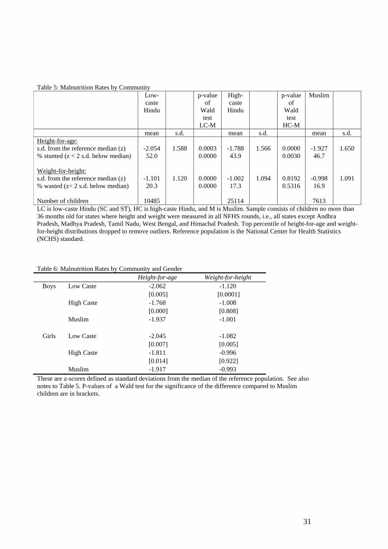
Table 5: Malnutrition Rates by Community Low-

caste Hindu

p-value of

Wald test

LC-M

High-caste

Hindu

p-value of

Wald test

HC-M

Muslim

mean s.d. mean s.d. mean s.d. Height-for-age: s.d. from the reference median (z) -2.054 1.588 0.0003 -1.788 1.566 0.0000 -1.927 1.650 % stunted (z < 2 s.d. below median) 52.0 0.0000 43.9 0.0030 46.7 Weight-for-height: s.d. from the reference median (z) -1.101 1.120 0.0000 -1.002 1.094 0.8192 -0.998 1.091 % wasted (z< 2 s.d. below median) 20.3 0.0000 17.3 0.5316 16.9 Number of children 10485 25114 7613 LC is low-caste Hindu (SC and ST), HC is high-caste Hindu, and M is Muslim. Sample consists of children no more than 36 months old for states where height and weight were measured in all NFHS rounds, i.e., all states except Andhra Pradesh, Madhya Pradesh, Tamil Nadu, West Bengal, and Himachal Pradesh. Top percentile of height-for-age and weight-for-height distributions dropped to remove outliers. Reference population is the National Center for Health Statistics (NCHS) standard. Table 6: Malnutrition Rates by Community and Gender Height-for-age Weight-for-height

Boys Low Caste -2.062 -1.120 [0.005] [0.0001] High Caste -1.768 -1.008 [0.000] [0.808] Muslim -1.937 -1.001

Girls Low Caste -2.045 -1.082 [0.007] [0.005] High Caste -1.811 -0.996 [0.014] [0.922] Muslim -1.917 -0.993

These are z-scores defined as standard deviations from the median of the reference population. See also notes to Table 5. P-values of a Wald test for the significance of the difference compared to Muslim children are in brackets.

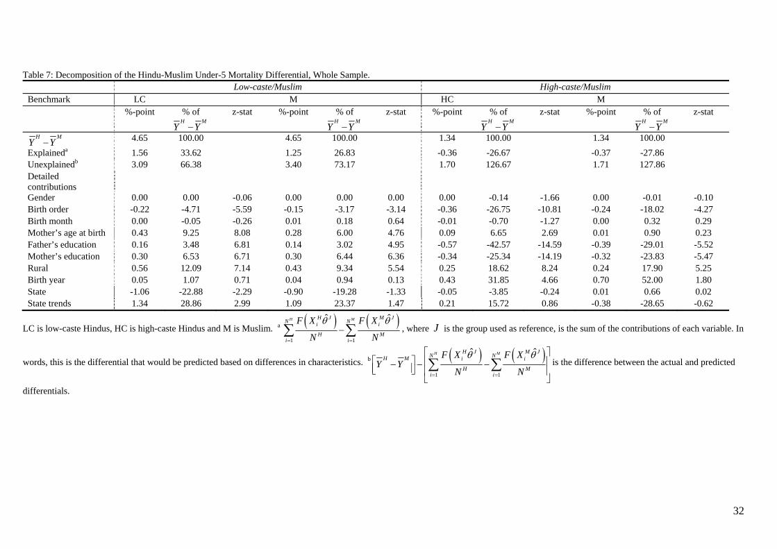
32

Table 7: Decomposition of the Hindu-Muslim Under-5 Mortality Differential, Whole Sample. Low-caste/Muslim High-caste/Muslim Benchmark LC M HC M %-point % of

H MY Y−

z-stat %-point % of H M

Y Y−z-stat %-point % of

H MY Y−


Y Y−z-stat

H MY Y− 4.65 100.00 4.65 100.00 1.34 100.00 1.34 100.00 Explaineda 1.56 33.62 1.25 26.83 -0.36 -26.67 -0.37 -27.86 Unexplainedb 3.09 66.38 3.40 73.17 1.70 126.67 1.71 127.86 Detailed contributions

Gender 0.00 0.00 -0.06 0.00 0.00 0.00 0.00 -0.14 -1.66 0.00 -0.01 -0.10 Birth order -0.22 -4.71 -5.59 -0.15 -3.17 -3.14 -0.36 -26.75 -10.81 -0.24 -18.02 -4.27 Birth month 0.00 -0.05 -0.26 0.01 0.18 0.64 -0.01 -0.70 -1.27 0.00 0.32 0.29 Mother’s age at birth 0.43 9.25 8.08 0.28 6.00 4.76 0.09 6.65 2.69 0.01 0.90 0.23 Father’s education 0.16 3.48 6.81 0.14 3.02 4.95 -0.57 -42.57 -14.59 -0.39 -29.01 -5.52 Mother’s education 0.30 6.53 6.71 0.30 6.44 6.36 -0.34 -25.34 -14.19 -0.32 -23.83 -5.47 Rural 0.56 12.09 7.14 0.43 9.34 5.54 0.25 18.62 8.24 0.24 17.90 5.25 Birth year 0.05 1.07 0.71 0.04 0.94 0.13 0.43 31.85 4.66 0.70 52.00 1.80 State -1.06 -22.88 -2.29 -0.90 -19.28 -1.33 -0.05 -3.85 -0.24 0.01 0.66 0.02 State trends 1.34 28.86 2.99 1.09 23.37 1.47 0.21 15.72 0.86 -0.38 -28.65 -0.62

LC is low-caste Hindus, HC is high-caste Hindus and M is Muslim. a ( ) ( )1 1

ˆ ˆH MH J M JN Ni i

H Mi i

F X F X

N N

θ θ

= =

−∑ ∑ , where J is the group used as reference, is the sum of the contributions of each variable. In

words, this is the differential that would be predicted based on differences in characteristics. b ( ) ( )1 1

ˆ ˆH MH J M JN NH M i i

H Mi i

F X F XY Y

N N

θ θ

= =

⎡ ⎤⎡ ⎤ ⎢ ⎥− − −⎢ ⎥⎣ ⎦ ⎢ ⎥

⎣ ⎦∑ ∑ is the difference between the actual and predicted

differentials.

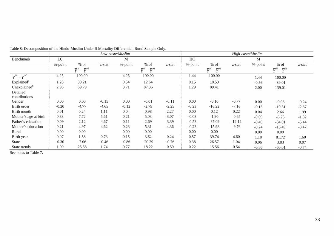
33

Table 8: Decomposition of the Hindu-Muslim Under-5 Mortality Differential, Rural Sample Only. Low-caste/Muslim High-caste/Muslim Benchmark LC M HC M %-point % of

H MY Y−



H MY Y−


Y Y−z-stat

H MY Y− 4.25 100.00 4.25 100.00 1.44 100.00 1.44 100.00 Explaineda 1.28 30.21 0.54 12.64 0.15 10.59 -0.56 -39.01 Unexplainedb 2.96 69.79 3.71 87.36 1.29 89.41 2.00 139.01 Detailed contributions

Gender 0.00 0.00 -0.15 0.00 -0.01 -0.11 0.00 -0.10 -0.77 0.00 -0.03 -0.24 Birth order -0.20 -4.77 -4.65 -0.12 -2.79 -2.25 -0.23 -16.22 -7.16 -0.15 -10.31 -2.67 Birth month 0.01 0.24 1.11 0.04 0.98 2.27 0.00 0.12 0.22 0.04 2.66 1.99 Mother’s age at birth 0.33 7.72 5.61 0.21 5.03 3.07 -0.03 -1.90 -0.65 -0.09 -6.25 -1.32 Father’s education 0.09 2.12 4.67 0.11 2.69 3.39 -0.53 -37.09 -12.12 -0.49 -34.01 -5.44 Mother’s education 0.21 4.97 4.62 0.23 5.31 4.36 -0.23 -15.98 -9.76 -0.24 -16.49 -3.47 Rural 0.00 0.00 0.00 0.00 0.00 0.00 0.00 0.00 Birth year 0.07 1.58 0.73 0.15 3.62 0.24 0.57 39.74 4.60 1.18 81.72 1.60 State -0.30 -7.06 -0.46 -0.86 -20.29 -0.76 0.38 26.57 1.04 0.06 3.83 0.07 State trends 1.09 25.58 1.74 0.77 18.22 0.59 0.22 15.56 0.54 -0.86 -60.01 -0.74

See notes to Table 7.

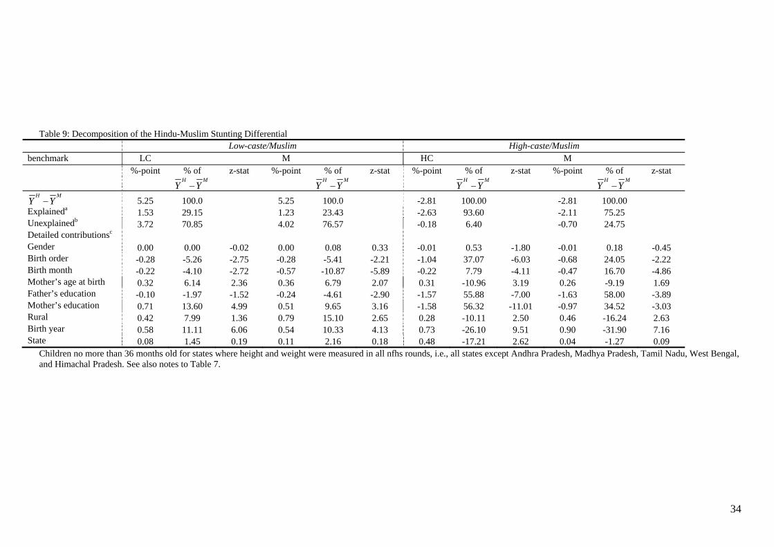
34

Table 9: Decomposition of the Hindu-Muslim Stunting Differential Low-caste/Muslim High-caste/Muslim benchmark LC M HC M %-point % of

H MY Y−



H MY Y−


Y Y−z-stat

H MY Y− 5.25 100.0 5.25 100.0 -2.81 100.00 -2.81 100.00 Explaineda 1.53 29.15 1.23 23.43 -2.63 93.60 -2.11 75.25 Unexplainedb 3.72 70.85 4.02 76.57 -0.18 6.40 -0.70 24.75 Detailed contributionsc Gender 0.00 0.00 -0.02 0.00 0.08 0.33 -0.01 0.53 -1.80 -0.01 0.18 -0.45 Birth order -0.28 -5.26 -2.75 -0.28 -5.41 -2.21 -1.04 37.07 -6.03 -0.68 24.05 -2.22 Birth month -0.22 -4.10 -2.72 -0.57 -10.87 -5.89 -0.22 7.79 -4.11 -0.47 16.70 -4.86 Mother’s age at birth 0.32 6.14 2.36 0.36 6.79 2.07 0.31 -10.96 3.19 0.26 -9.19 1.69 Father’s education -0.10 -1.97 -1.52 -0.24 -4.61 -2.90 -1.57 55.88 -7.00 -1.63 58.00 -3.89 Mother’s education 0.71 13.60 4.99 0.51 9.65 3.16 -1.58 56.32 -11.01 -0.97 34.52 -3.03 Rural 0.42 7.99 1.36 0.79 15.10 2.65 0.28 -10.11 2.50 0.46 -16.24 2.63 Birth year 0.58 11.11 6.06 0.54 10.33 4.13 0.73 -26.10 9.51 0.90 -31.90 7.16 State 0.08 1.45 0.19 0.11 2.16 0.18 0.48 -17.21 2.62 0.04 -1.27 0.09

Children no more than 36 months old for states where height and weight were measured in all nfhs rounds, i.e., all states except Andhra Pradesh, Madhya Pradesh, Tamil Nadu, West Bengal, and Himachal Pradesh. See also notes to Table 7.

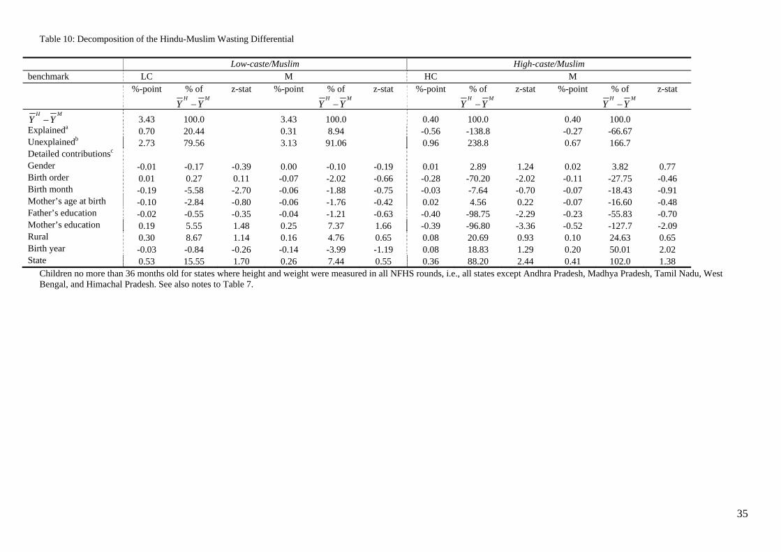
35

Table 10: Decomposition of the Hindu-Muslim Wasting Differential

Low-caste/Muslim High-caste/Muslim benchmark LC M HC M %-point % of

H MY Y−



H MY Y−


Y Y−z-stat

H MY Y− 3.43 100.0 3.43 100.0 0.40 100.0 0.40 100.0 Explaineda 0.70 20.44 0.31 8.94 -0.56 -138.8 -0.27 -66.67 Unexplainedb 2.73 79.56 3.13 91.06 0.96 238.8 0.67 166.7 Detailed contributionsc Gender -0.01 -0.17 -0.39 0.00 -0.10 -0.19 0.01 2.89 1.24 0.02 3.82 0.77 Birth order 0.01 0.27 0.11 -0.07 -2.02 -0.66 -0.28 -70.20 -2.02 -0.11 -27.75 -0.46 Birth month -0.19 -5.58 -2.70 -0.06 -1.88 -0.75 -0.03 -7.64 -0.70 -0.07 -18.43 -0.91 Mother’s age at birth -0.10 -2.84 -0.80 -0.06 -1.76 -0.42 0.02 4.56 0.22 -0.07 -16.60 -0.48 Father’s education -0.02 -0.55 -0.35 -0.04 -1.21 -0.63 -0.40 -98.75 -2.29 -0.23 -55.83 -0.70 Mother’s education 0.19 5.55 1.48 0.25 7.37 1.66 -0.39 -96.80 -3.36 -0.52 -127.7 -2.09 Rural 0.30 8.67 1.14 0.16 4.76 0.65 0.08 20.69 0.93 0.10 24.63 0.65 Birth year -0.03 -0.84 -0.26 -0.14 -3.99 -1.19 0.08 18.83 1.29 0.20 50.01 2.02 State 0.53 15.55 1.70 0.26 7.44 0.55 0.36 88.20 2.44 0.41 102.0 1.38

Children no more than 36 months old for states where height and weight were measured in all NFHS rounds, i.e., all states except Andhra Pradesh, Madhya Pradesh, Tamil Nadu, West Bengal, and Himachal Pradesh. See also notes to Table 7.

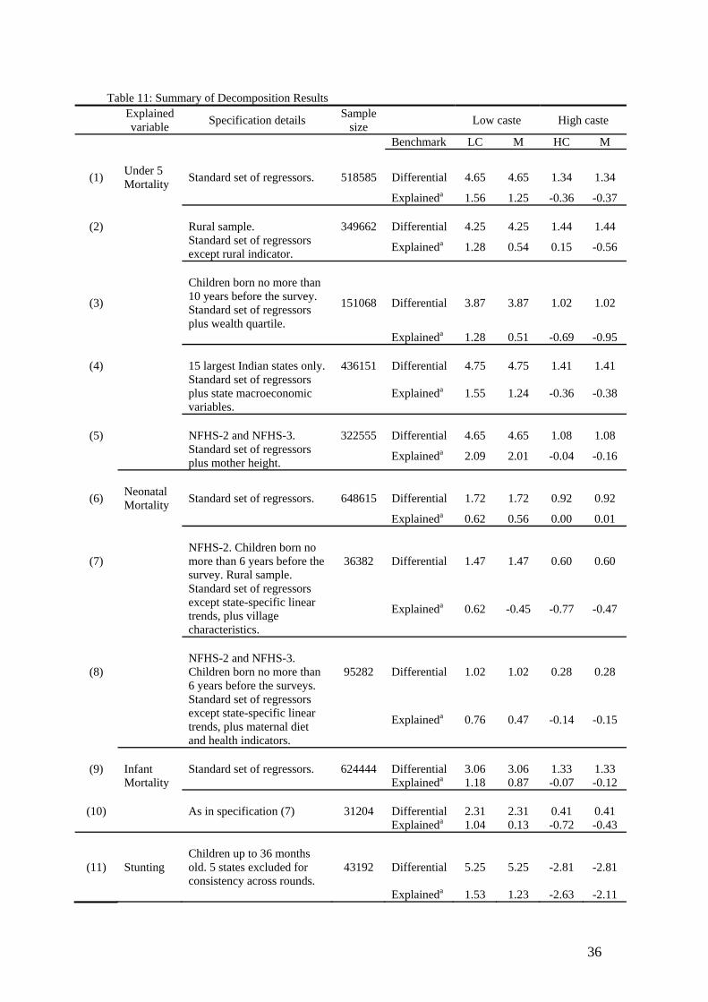
36

Table 11: Summary of Decomposition Results

Explained variable Specification details Sample

size Low caste High caste

Benchmark LC M HC M

(1) Under 5 Mortality Standard set of regressors. 518585 Differential 4.65 4.65 1.34 1.34

Explaineda 1.56 1.25 -0.36 -0.37

(2) Rural sample. 349662 Differential 4.25 4.25 1.44 1.44

Standard set of regressors except rural indicator. Explaineda 1.28 0.54 0.15 -0.56

(3)

Children born no more than 10 years before the survey. Standard set of regressors plus wealth quartile.

151068

Differential 3.87 3.87 1.02 1.02

Explaineda 1.28 0.51 -0.69 -0.95

(4) 15 largest Indian states only. 436151 Differential 4.75 4.75 1.41 1.41

Standard set of regressors plus state macroeconomic variables.

Explaineda 1.55 1.24 -0.36 -0.38

(5) NFHS-2 and NFHS-3. 322555 Differential 4.65 4.65 1.08 1.08

Standard set of regressors plus mother height. Explaineda 2.09 2.01 -0.04 -0.16

(6) Neonatal Mortality Standard set of regressors. 648615 Differential 1.72 1.72 0.92 0.92

Explaineda 0.62 0.56 0.00 0.01

(7) NFHS-2. Children born no more than 6 years before the survey. Rural sample.

36382 Differential 1.47 1.47 0.60 0.60

Standard set of regressors except state-specific linear trends, plus village characteristics.

Explaineda 0.62 -0.45 -0.77 -0.47

(8) NFHS-2 and NFHS-3. Children born no more than 6 years before the surveys.

95282 Differential 1.02 1.02 0.28 0.28

Standard set of regressors except state-specific linear trends, plus maternal diet and health indicators.

Explaineda 0.76 0.47 -0.14 -0.15

(9) Infant

Mortality Standard set of regressors.

624444

Differential 3.06 3.06 1.33 1.33

Explaineda 1.18 0.87 -0.07 -0.12

(10) As in specification (7) 31204 Differential 2.31 2.31 0.41 0.41 Explaineda 1.04 0.13 -0.72 -0.43

(11) Stunting Children up to 36 months old. 5 states excluded for consistency across rounds.

43192

Differential 5.25 5.25 -2.81 -2.81

Explaineda 1.53 1.23 -2.63 -2.11

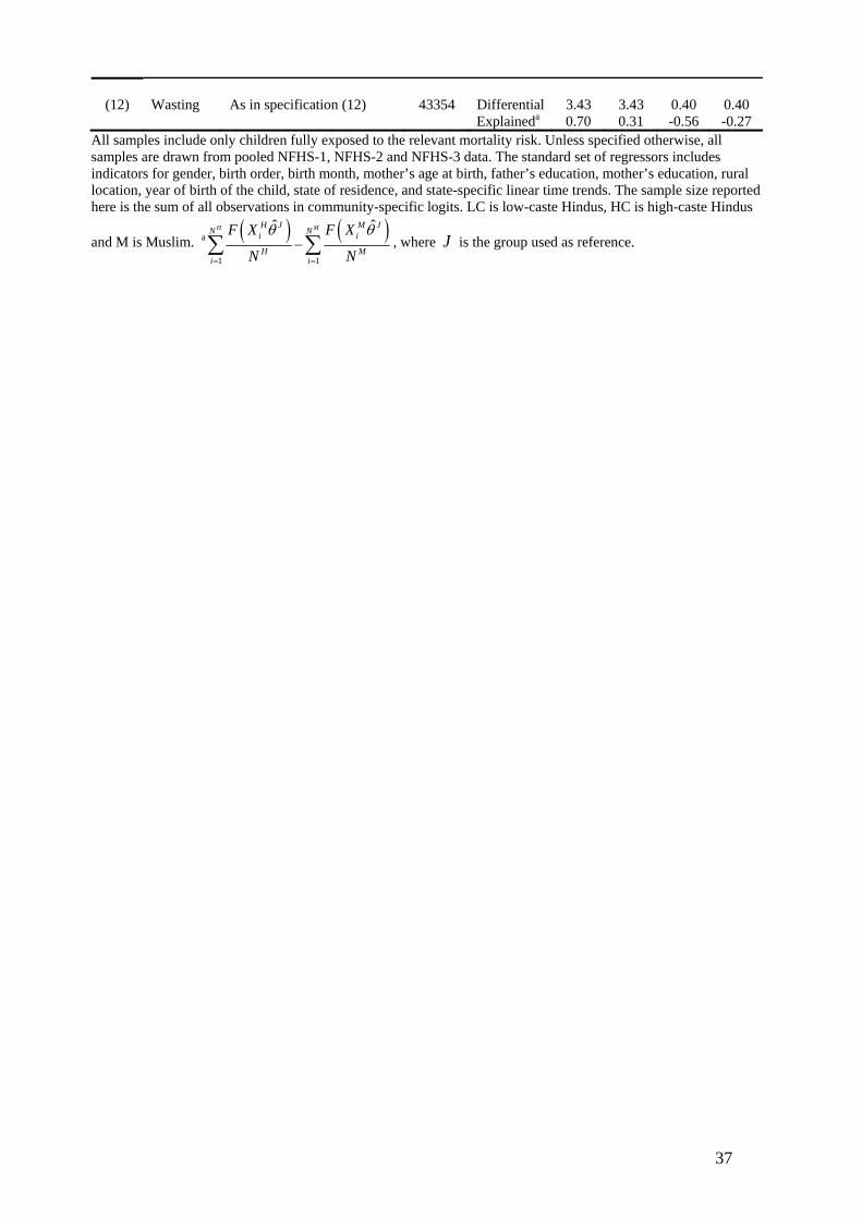
37

(12) Wasting As in specification (12) 43354 Differential 3.43 3.43 0.40 0.40

Explaineda 0.70 0.31 -0.56 -0.27 All samples include only children fully exposed to the relevant mortality risk. Unless specified otherwise, all samples are drawn from pooled NFHS-1, NFHS-2 and NFHS-3 data. The standard set of regressors includes indicators for gender, birth order, birth month, mother’s age at birth, father’s education, mother’s education, rural location, year of birth of the child, state of residence, and state-specific linear time trends. The sample size reported here is the sum of all observations in community-specific logits. LC is low-caste Hindus, HC is high-caste Hindus

and M is Muslim. a ( ) ( )1 1

ˆ ˆH MH J M JN Ni i

H Mi i

F X F X

N N

θ θ

= =

−∑ ∑ , where J is the group used as reference.

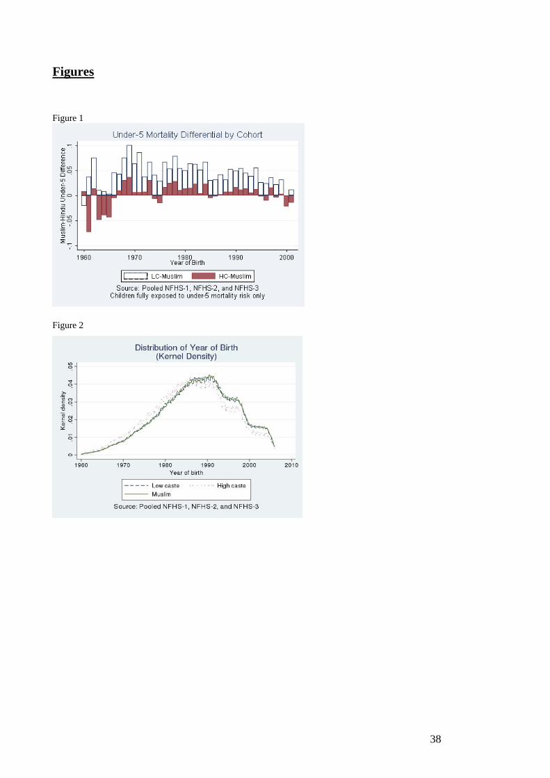
38

Figures Figure 1

Figure 2

39

Appendix Appendix Table 1: Summary Statistics LC

(%) p-value of Wald test

LC-Ma

Obs. HC (%)

p-value of Wald test HC-Ma

Obs. M (%)

Obs.

Female 48.13 0.459 163387 47.92 0.063 388634 48.30 101475 Child birth order: First childb 28.00 163387 31.30 388634 25.60 101475 Second child 23.92 163387 26.26 388634 22.01 101475 Third child 18.32 163387 18.06 388634 17.18 101475 Fourth or later child 29.76 163387 24.38 388634 35.21 101475 Month of birth: January b 7.20 0.7473 163387 7.30 0.6227 388634 7.24 101475 February 6.66 0.1502 163387 6.59 0.0280 388634 6.86 101475 March 7.92 0.6911 163387 7.58 0.0026 388634 7.98 101475 April 7.98 0.0001 163387 7.54 388634 8.58 101475 May 8.12 0.0001 163387 8.01 388634 8.74 101475 June 8.81 0.0079 163387 8.54 388634 9.24 101475 July 8.81 163387 8.91 388634 8.04 101475 August 10.25 163387 10.50 388634 9.11 101475 September 8.57 0.5006 163387 8.85 0.0048 388634 8.47 101475 October 9.54 163387 9.81 388634 8.78 101475 November 8.78 0.7594 163387 8.88 0.7290 388634 8.83 101475 December 7.37 163387 7.49 388634 8.14 101475 Maternal age at birth: 9-15 6.19 163387 4.52 388634 5.13 101475 16-18 19.12 163387 16.97 0.8395 388634 17.02 101475 19-24 b 44.34 163387 47.39 388634 43.13 101475 25-30 22.05 163387 23.45 0.0093 388634 24.01 101475 31-49 8.30 163387 7.66 388634 10.71 101475 Father’s education: No schooling b 50.03 162354 28.51 386677 43.56 100558 Primary 21.62 162354 22.25 0.0010 386677 24.08 100558 Secondary 23.96 162354 37.29 386677 27.16 100558 Higher 4.38 0.0031 162354 11.95 386677 5.19 100558 Mother’s education: No schooling b 80.26 163227 58.17 388106 68.52 101265 Incomplete primary 7.27 163227 11.40 0.4243 388106 11.75 101265 Complete primary 3.23 163227 5.75 388106 4.76 101265 Incomplete secondary 7.73 163227 17.96 388106 12.19 101265 Complete secondary and higher

1.51 163227 6.71 388106 2.78 101265

Rural 83.08 163387 74.29 388634 64.82 101475 Urbanb 16.92 163387 25.71 388634 35.18 101475 Year of birth 1987.5 0.6253 163387 1986.1 388634 1987.6 101475 State: Andhra Pradeshb 6.08 0.0261 163387 8.49 388634 4.70 101475 Assam 2.53 163387 1.89 388634 6.06 101475 Bihar 9.93 0.0008 163387 11.94 0.0796 388634 14.04 101475 Goa 0.03 0.0005 163387 0.11 388634 0.06 101475 Gujarat 5.41 163387 5.36 388634 3.01 101475 Haryana 1.92 163387 2.20 388634 0.84 101475 Himachal Pradesh 0.60 163387 0.69 388634 0.07 101475 Jammu and Kashmir 0.45 163387 0.38 388634 2.69 101475 Karnataka 4.69 0.6634 163387 5.48 0.0325 388634 4.47 101475 Kerala 0.89 163387 1.79 388634 5.81 101475 Madhya Pradesh 13.70 163387 8.24 388634 3.42 101475

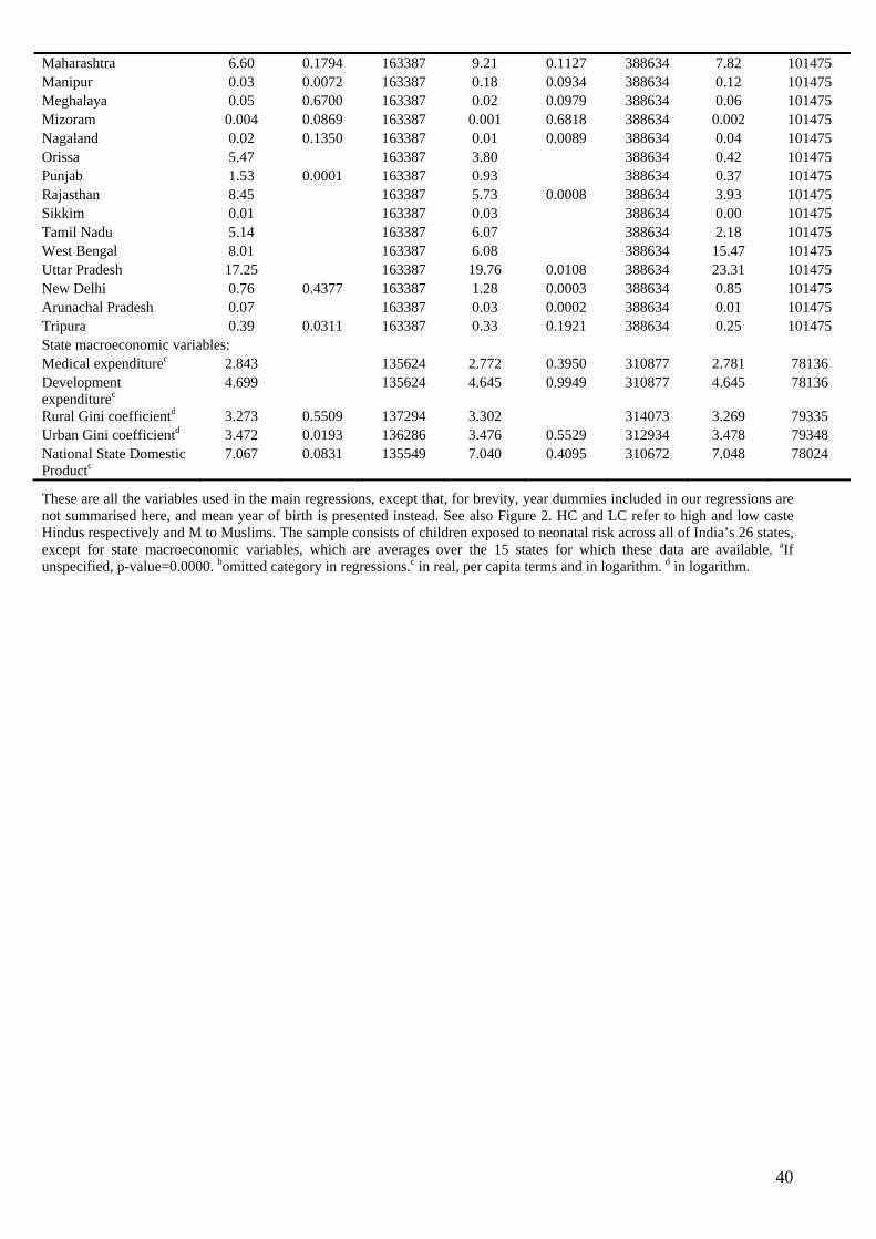
40

Maharashtra 6.60 0.1794 163387 9.21 0.1127 388634 7.82 101475 Manipur 0.03 0.0072 163387 0.18 0.0934 388634 0.12 101475 Meghalaya 0.05 0.6700 163387 0.02 0.0979 388634 0.06 101475 Mizoram 0.004 0.0869 163387 0.001 0.6818 388634 0.002 101475 Nagaland 0.02 0.1350 163387 0.01 0.0089 388634 0.04 101475 Orissa 5.47 163387 3.80 388634 0.42 101475 Punjab 1.53 0.0001 163387 0.93 388634 0.37 101475 Rajasthan 8.45 163387 5.73 0.0008 388634 3.93 101475 Sikkim 0.01 163387 0.03 388634 0.00 101475 Tamil Nadu 5.14 163387 6.07 388634 2.18 101475 West Bengal 8.01 163387 6.08 388634 15.47 101475 Uttar Pradesh 17.25 163387 19.76 0.0108 388634 23.31 101475 New Delhi 0.76 0.4377 163387 1.28 0.0003 388634 0.85 101475 Arunachal Pradesh 0.07 163387 0.03 0.0002 388634 0.01 101475 Tripura 0.39 0.0311 163387 0.33 0.1921 388634 0.25 101475 State macroeconomic variables: Medical expenditurec 2.843 135624 2.772 0.3950 310877 2.781 78136 Development expenditurec

4.699 135624 4.645 0.9949 310877 4.645 78136

Rural Gini coefficientd 3.273 0.5509 137294 3.302 314073 3.269 79335 Urban Gini coefficientd 3.472 0.0193 136286 3.476 0.5529 312934 3.478 79348 National State Domestic Productc

7.067 0.0831 135549 7.040 0.4095 310672 7.048 78024

These are all the variables used in the main regressions, except that, for brevity, year dummies included in our regressions are not summarised here, and mean year of birth is presented instead. See also Figure 2. HC and LC refer to high and low caste Hindus respectively and M to Muslims. The sample consists of children exposed to neonatal risk across all of India’s 26 states, except for state macroeconomic variables, which are averages over the 15 states for which these data are available. aIf unspecified, p-value=0.0000. bomitted category in regressions.c in real, per capita terms and in logarithm. d in logarithm.

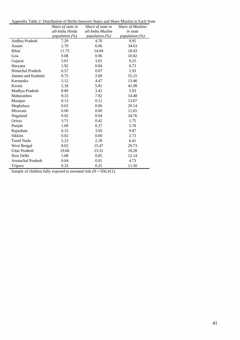
41

Appendix Table 2: Distribution of Births between States and Share Muslim in Each State

Share of state in all-India Hindu population (%)

Share of state in all-India Muslim population (%)

Share of Muslims in state

population (%) Andhra Pradesh 7.29 4.70 9.95 Assam 2.70 6.06 34.63 Bihar 11.75 14.04 18.43 Goa 0.08 0.06 10.82 Gujarat 5.01 3.01 9.25 Haryana 1.92 0.84 6.73 Himachal Pradesh 0.57 0.07 1.93 Jammu and Kashmir 0.75 2.69 55.15 Karnataka 5.12 4.47 13.46 Kerala 2.18 5.81 41.08 Madhya Pradesh 8.89 3.42 5.93 Maharashtra 8.33 7.82 14.48 Manipur 0.13 0.12 13.87 Meghalaya 0.03 0.06 29.14 Mizoram 0.00 0.00 11.65 Nagaland 0.02 0.04 34.76 Orissa 3.71 0.42 1.75 Punjab 1.00 0.37 5.78 Rajasthan 6.15 3.93 9.87 Sikkim 0.02 0.00 2.73 Tamil Nadu 5.23 2.18 6.41 West Bengal 8.02 15.47 29.73 Uttar Pradesh 19.66 23.31 18.28 New Delhi 1.08 0.85 12.14 Arunachal Pradesh 0.04 0.01 4.73 Tripura 0.33 0.25 11.50 Sample of children fully exposed to neonatal risk (N = 656,411).

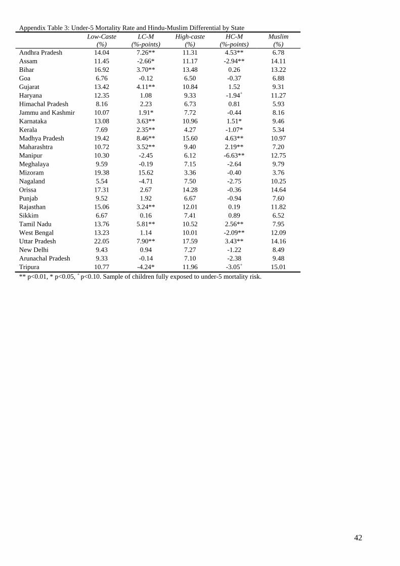
42

Appendix Table 3: Under-5 Mortality Rate and Hindu-Muslim Differential by State Low-Caste

(%) LC-M

(%-points) High-caste

(%) HC-M

(%-points) Muslim

(%) Andhra Pradesh 14.04 7.26** 11.31 4.53** 6.78 Assam 11.45 -2.66* 11.17 -2.94** 14.11 Bihar 16.92 3.70** 13.48 0.26 13.22 Goa 6.76 -0.12 6.50 -0.37 6.88 Gujarat 13.42 4.11** 10.84 1.52 9.31 Haryana 12.35 1.08 9.33 -1.94+ 11.27 Himachal Pradesh 8.16 2.23 6.73 0.81 5.93 Jammu and Kashmir 10.07 1.91* 7.72 -0.44 8.16 Karnataka 13.08 3.63** 10.96 1.51* 9.46 Kerala 7.69 2.35** 4.27 -1.07* 5.34 Madhya Pradesh 19.42 8.46** 15.60 4.63** 10.97 Maharashtra 10.72 3.52** 9.40 2.19** 7.20 Manipur 10.30 -2.45 6.12 -6.63** 12.75 Meghalaya 9.59 -0.19 7.15 -2.64 9.79 Mizoram 19.38 15.62 3.36 -0.40 3.76 Nagaland 5.54 -4.71 7.50 -2.75 10.25 Orissa 17.31 2.67 14.28 -0.36 14.64 Punjab 9.52 1.92 6.67 -0.94 7.60 Rajasthan 15.06 3.24** 12.01 0.19 11.82 Sikkim 6.67 0.16 7.41 0.89 6.52 Tamil Nadu 13.76 5.81** 10.52 2.56** 7.95 West Bengal 13.23 1.14 10.01 -2.09** 12.09 Uttar Pradesh 22.05 7.90** 17.59 3.43** 14.16 New Delhi 9.43 0.94 7.27 -1.22 8.49 Arunachal Pradesh 9.33 -0.14 7.10 -2.38 9.48 Tripura 10.77 -4.24* 11.96 -3.05+ 15.01 ** p<0.01, * p<0.05, + p<0.10. Sample of children fully exposed to under-5 mortality risk.

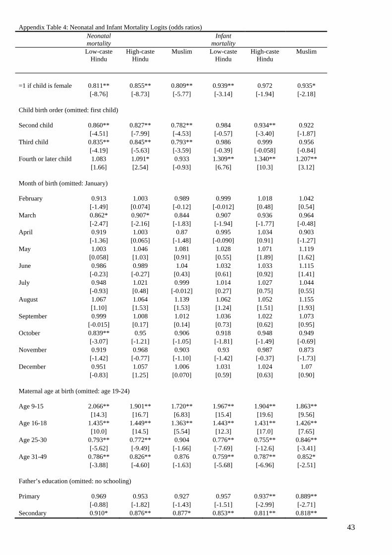
43

Appendix Table 4: Neonatal and Infant Mortality Logits (odds ratios) Neonatal

mortality Infant

mortality

Low-caste Hindu

High-caste Hindu

Muslim

Low-caste Hindu

High-caste Hindu

Muslim

=1 if child is female 0.811** 0.855** 0.809** 0.939** 0.972 0.935* [-8.76] [-8.73] [-5.77] [-3.14] [-1.94] [-2.18] Child birth order (omitted: first child) Second child 0.860** 0.827** 0.782** 0.984 0.934** 0.922 [-4.51] [-7.99] [-4.53] [-0.57] [-3.40] [-1.87] Third child 0.835** 0.845** 0.793** 0.986 0.999 0.956 [-4.19] [-5.63] [-3.59] [-0.39] [-0.058] [-0.84] Fourth or later child 1.083 1.091* 0.933 1.309** 1.340** 1.207** [1.66] [2.54] [-0.93] [6.76] [10.3] [3.12] Month of birth (omitted: January) February 0.913 1.003 0.989 0.999 1.018 1.042 [-1.49] [0.074] [-0.12] [-0.012] [0.48] [0.54] March 0.862* 0.907* 0.844 0.907 0.936 0.964 [-2.47] [-2.16] [-1.83] [-1.94] [-1.77] [-0.48] April 0.919 1.003 0.87 0.995 1.034 0.903 [-1.36] [0.065] [-1.48] [-0.090] [0.91] [-1.27] May 1.003 1.046 1.081 1.028 1.071 1.119 [0.058] [1.03] [0.91] [0.55] [1.89] [1.62] June 0.986 0.989 1.04 1.032 1.033 1.115 [-0.23] [-0.27] [0.43] [0.61] [0.92] [1.41] July 0.948 1.021 0.999 1.014 1.027 1.044 [-0.93] [0.48] [-0.012] [0.27] [0.75] [0.55] August 1.067 1.064 1.139 1.062 1.052 1.155 [1.10] [1.53] [1.53] [1.24] [1.51] [1.93] September 0.999 1.008 1.012 1.036 1.022 1.073 [-0.015] [0.17] [0.14] [0.73] [0.62] [0.95] October 0.839** 0.95 0.906 0.918 0.948 0.949 [-3.07] [-1.21] [-1.05] [-1.81] [-1.49] [-0.69] November 0.919 0.968 0.903 0.93 0.987 0.873 [-1.42] [-0.77] [-1.10] [-1.42] [-0.37] [-1.73] December 0.951 1.057 1.006 1.031 1.024 1.07 [-0.83] [1.25] [0.070] [0.59] [0.63] [0.90] Maternal age at birth (omitted: age 19-24) Age 9-15 2.066** 1.901** 1.720** 1.967** 1.904** 1.863** [14.3] [16.7] [6.83] [15.4] [19.6] [9.56] Age 16-18 1.435** 1.449** 1.363** 1.443** 1.431** 1.426** [10.0] [14.5] [5.54] [12.3] [17.0] [7.65] Age 25-30 0.793** 0.772** 0.904 0.776** 0.755** 0.846** [-5.62] [-9.49] [-1.66] [-7.69] [-12.6] [-3.41] Age 31-49 0.786** 0.826** 0.876 0.759** 0.787** 0.852* [-3.88] [-4.60] [-1.63] [-5.68] [-6.96] [-2.51] Father’s education (omitted: no schooling)

Primary 0.969 0.953 0.927 0.957 0.937** 0.889** [-0.88] [-1.82] [-1.43] [-1.51] [-2.99] [-2.71] Secondary 0.910* 0.876** 0.877* 0.853** 0.811** 0.818**

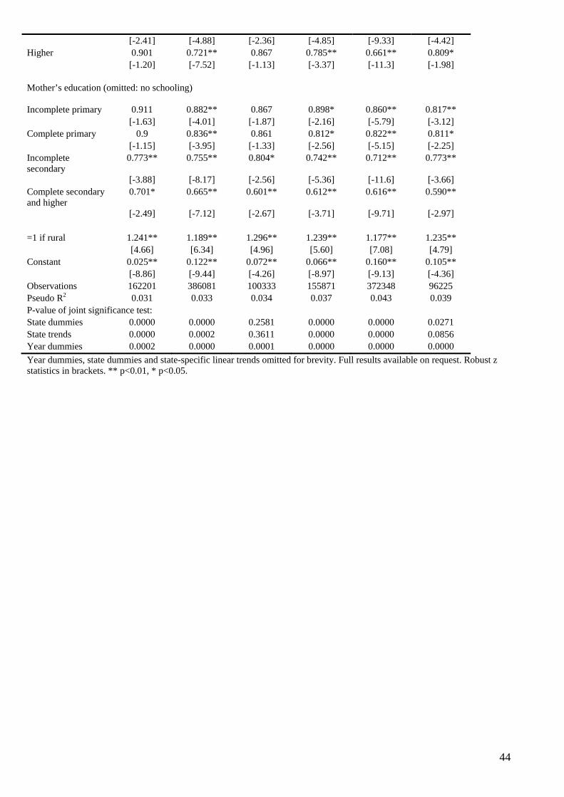
44

[-2.41] [-4.88] [-2.36] [-4.85] [-9.33] [-4.42] Higher 0.901 0.721** 0.867 0.785** 0.661** 0.809* [-1.20] [-7.52] [-1.13] [-3.37] [-11.3] [-1.98] Mother’s education (omitted: no schooling)

Incomplete primary 0.911 0.882** 0.867 0.898* 0.860** 0.817** [-1.63] [-4.01] [-1.87] [-2.16] [-5.79] [-3.12] Complete primary 0.9 0.836** 0.861 0.812* 0.822** 0.811* [-1.15] [-3.95] [-1.33] [-2.56] [-5.15] [-2.25] Incomplete secondary

0.773** 0.755** 0.804* 0.742** 0.712** 0.773**

[-3.88] [-8.17] [-2.56] [-5.36] [-11.6] [-3.66] Complete secondary and higher

0.701* 0.665** 0.601** 0.612** 0.616** 0.590**

[-2.49] [-7.12] [-2.67] [-3.71] [-9.71] [-2.97] =1 if rural 1.241** 1.189** 1.296** 1.239** 1.177** 1.235** [4.66] [6.34] [4.96] [5.60] [7.08] [4.79] Constant 0.025** 0.122** 0.072** 0.066** 0.160** 0.105** [-8.86] [-9.44] [-4.26] [-8.97] [-9.13] [-4.36] Observations 162201 386081 100333 155871 372348 96225 Pseudo R2 0.031 0.033 0.034 0.037 0.043 0.039 P-value of joint significance test: State dummies 0.0000 0.0000 0.2581 0.0000 0.0000 0.0271 State trends 0.0000 0.0002 0.3611 0.0000 0.0000 0.0856 Year dummies 0.0002 0.0000 0.0001 0.0000 0.0000 0.0000 Year dummies, state dummies and state-specific linear trends omitted for brevity. Full results available on request. Robust z statistics in brackets. ** p<0.01, * p<0.05.

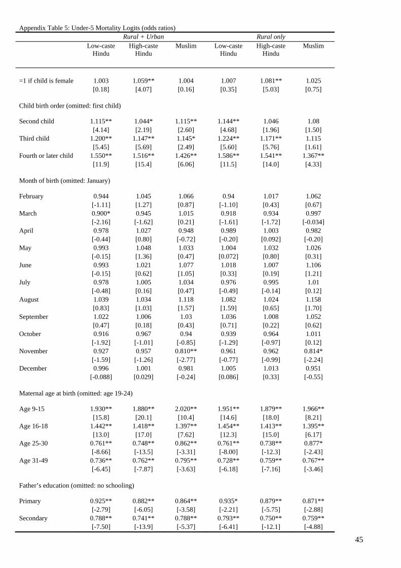
45

Appendix Table 5: Under-5 Mortality Logits (odds ratios) Rural + Urban Rural only Low-caste

Hindu High-caste

Hindu Muslim

Low-caste

Hindu High-caste

Hindu Muslim

=1 if child is female 1.003 1.059** 1.004 1.007 1.081** 1.025 [0.18] [4.07] [0.16] [0.35] [5.03] [0.75] Child birth order (omitted: first child) Second child 1.115** 1.044* 1.115** 1.144** 1.046 1.08 [4.14] [2.19] [2.60] [4.68] [1.96] [1.50] Third child 1.200** 1.147** 1.145* 1.224** 1.171** 1.115 [5.45] [5.69] [2.49] [5.60] [5.76] [1.61] Fourth or later child 1.550** 1.516** 1.426** 1.586** 1.541** 1.367** [11.9] [15.4] [6.06] [11.5] [14.0] [4.33] Month of birth (omitted: January) February 0.944 1.045 1.066 0.94 1.017 1.062 [-1.11] [1.27] [0.87] [-1.10] [0.43] [0.67] March 0.900* 0.945 1.015 0.918 0.934 0.997 [-2.16] [-1.62] [0.21] [-1.61] [-1.72] [-0.034] April 0.978 1.027 0.948 0.989 1.003 0.982 [-0.44] [0.80] [-0.72] [-0.20] [0.092] [-0.20] May 0.993 1.048 1.033 1.004 1.032 1.026 [-0.15] [1.36] [0.47] [0.072] [0.80] [0.31] June 0.993 1.021 1.077 1.018 1.007 1.106 [-0.15] [0.62] [1.05] [0.33] [0.19] [1.21] July 0.978 1.005 1.034 0.976 0.995 1.01 [-0.48] [0.16] [0.47] [-0.49] [-0.14] [0.12] August 1.039 1.034 1.118 1.082 1.024 1.158 [0.83] [1.03] [1.57] [1.59] [0.65] [1.70] September 1.022 1.006 1.03 1.036 1.008 1.052 [0.47] [0.18] [0.43] [0.71] [0.22] [0.62] October 0.916 0.967 0.94 0.939 0.964 1.011 [-1.92] [-1.01] [-0.85] [-1.29] [-0.97] [0.12] November 0.927 0.957 0.810** 0.961 0.962 0.814* [-1.59] [-1.26] [-2.77] [-0.77] [-0.99] [-2.24] December 0.996 1.001 0.981 1.005 1.013 0.951 [-0.088] [0.029] [-0.24] [0.086] [0.33] [-0.55] Maternal age at birth (omitted: age 19-24) Age 9-15 1.930** 1.880** 2.020** 1.951** 1.879** 1.966** [15.8] [20.1] [10.4] [14.6] [18.0] [8.21] Age 16-18 1.442** 1.418** 1.397** 1.454** 1.413** 1.395** [13.0] [17.0] [7.62] [12.3] [15.0] [6.17] Age 25-30 0.761** 0.748** 0.862** 0.761** 0.738** 0.877* [-8.66] [-13.5] [-3.31] [-8.00] [-12.3] [-2.43] Age 31-49 0.736** 0.762** 0.795** 0.728** 0.759** 0.767** [-6.45] [-7.87] [-3.63] [-6.18] [-7.16] [-3.46] Father’s education (omitted: no schooling)

Primary 0.925** 0.882** 0.864** 0.935* 0.879** 0.871** [-2.79] [-6.05] [-3.58] [-2.21] [-5.75] [-2.88] Secondary 0.788** 0.741** 0.788** 0.793** 0.750** 0.759** [-7.50] [-13.9] [-5.37] [-6.41] [-12.1] [-4.88]

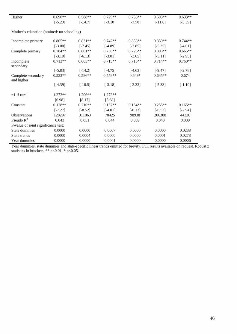
46

Higher 0.690** 0.588** 0.729** 0.755** 0.603** 0.633** [-5.23] [-14.7] [-3.18] [-3.58] [-11.6] [-3.39] Mother’s education (omitted: no schooling)

Incomplete primary 0.865** 0.831** 0.742** 0.853** 0.859** 0.744** [-3.00] [-7.45] [-4.89] [-2.85] [-5.35] [-4.01] Complete primary 0.784** 0.801** 0.750** 0.726** 0.803** 0.665** [-3.19] [-6.13] [-3.01] [-3.65] [-5.11] [-2.95] Incomplete secondary

0.713** 0.665** 0.715** 0.715** 0.714** 0.760**


0.533** 0.586** 0.558** 0.649* 0.635** 0.674

[-4.39] [-10.5] [-3.18] [-2.33] [-5.33] [-1.10] =1 if rural 1.272** 1.206** 1.273** [6.98] [8.17] [5.68] Constant 0.128** 0.210** 0.157** 0.154** 0.255** 0.165** [-7.27] [-8.52] [-4.01] [-6.13] [-6.53] [-2.94] Observations 128297 311863 78425 98938 206388 44336 Pseudo R2 0.043 0.051 0.044 0.039 0.043 0.039 P-value of joint significance test: State dummies 0.0000 0.0000 0.0007 0.0000 0.0000 0.0238 State trends 0.0000 0.0004 0.0000 0.0000 0.0001 0.0278 Year dummies 0.0000 0.0000 0.0001 0.0000 0.0000 0.0006 Year dummies, state dummies and state-specific linear trends omitted for brevity. Full results available on request. Robust z statistics in brackets. ** p<0.01, * p<0.05.

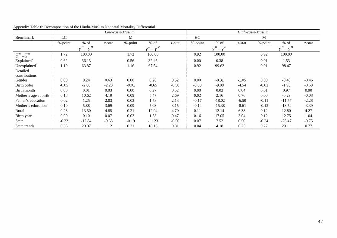
47

Appendix Table 6: Decomposition of the Hindu-Muslim Neonatal Mortality Differential Low-caste/Muslim High-caste/Muslim Benchmark LC M HC M %-point % of

H MY Y−



H MY Y−


Y Y−z-stat

H MY Y− 1.72 100.00 1.72 100.00 0.92 100.00 0.92 100.00 Explaineda 0.62 36.13 0.56 32.46 0.00 0.38 0.01 1.53 Unexplainedb 1.10 63.87 1.16 67.54 0.92 99.62 0.91 98.47 Detailed contributions

Gender 0.00 0.24 0.63 0.00 0.26 0.52 0.00 -0.31 -1.05 0.00 -0.40 -0.46 Birth order -0.05 -2.80 -2.20 -0.01 -0.65 -0.50 -0.08 -9.08 -4.54 -0.02 -1.93 -0.60 Birth month 0.00 0.01 0.03 0.00 0.27 0.52 0.00 0.02 0.04 0.01 0.97 0.90 Mother’s age at birth 0.18 10.62 4.10 0.09 5.47 2.69 0.02 2.16 0.76 0.00 -0.29 -0.08 Father’s education 0.02 1.25 2.03 0.03 1.53 2.13 -0.17 -18.02 -6.50 -0.11 -11.57 -2.28 Mother’s education 0.10 5.88 3.69 0.09 5.03 3.15 -0.14 -15.38 -8.61 -0.12 -13.54 -3.39 Rural 0.23 13.50 4.85 0.21 12.04 4.70 0.11 12.14 6.38 0.12 12.80 4.27 Birth year 0.00 0.10 0.07 0.03 1.53 0.47 0.16 17.05 3.04 0.12 12.75 1.04 State -0.22 -12.84 -0.68 -0.19 -11.23 -0.50 0.07 7.52 0.50 -0.24 -26.47 -0.75 State trends 0.35 20.07 1.12 0.31 18.13 0.81 0.04 4.18 0.25 0.27 29.11 0.77

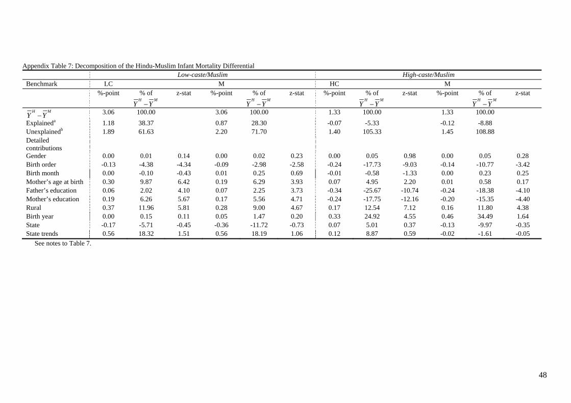
48

Appendix Table 7: Decomposition of the Hindu-Muslim Infant Mortality Differential Low-caste/Muslim High-caste/Muslim Benchmark LC M HC M %-point % of

H MY Y−



H MY Y−


Y Y−z-stat

H MY Y− 3.06 100.00 3.06 100.00 1.33 100.00 1.33 100.00 Explaineda 1.18 38.37 0.87 28.30 -0.07 -5.33 -0.12 -8.88 Unexplainedb 1.89 61.63 2.20 71.70 1.40 105.33 1.45 108.88 Detailed contributions

Gender 0.00 0.01 0.14 0.00 0.02 0.23 0.00 0.05 0.98 0.00 0.05 0.28 Birth order -0.13 -4.38 -4.34 -0.09 -2.98 -2.58 -0.24 -17.73 -9.03 -0.14 -10.77 -3.42 Birth month 0.00 -0.10 -0.43 0.01 0.25 0.69 -0.01 -0.58 -1.33 0.00 0.23 0.25 Mother’s age at birth 0.30 9.87 6.42 0.19 6.29 3.93 0.07 4.95 2.20 0.01 0.58 0.17 Father’s education 0.06 2.02 4.10 0.07 2.25 3.73 -0.34 -25.67 -10.74 -0.24 -18.38 -4.10 Mother’s education 0.19 6.26 5.67 0.17 5.56 4.71 -0.24 -17.75 -12.16 -0.20 -15.35 -4.40 Rural 0.37 11.96 5.81 0.28 9.00 4.67 0.17 12.54 7.12 0.16 11.80 4.38 Birth year 0.00 0.15 0.11 0.05 1.47 0.20 0.33 24.92 4.55 0.46 34.49 1.64 State -0.17 -5.71 -0.45 -0.36 -11.72 -0.73 0.07 5.01 0.37 -0.13 -9.97 -0.35 State trends 0.56 18.32 1.51 0.56 18.19 1.06 0.12 8.87 0.59 -0.02 -1.61 -0.05

See notes to Table 7.

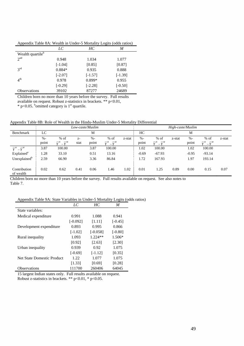
49

Appendix Table 8A: Wealth in Under-5 Mortality Logits (odds ratios) LC HC M Wealth quartileb 2nd 0.948 1.034 1.077 [-1.04] [0.85] [0.87] 3rd 0.884* 0.935 0.888 [-2.07] [-1.57] [-1.39] 4th 0.978 0.899* 0.955 [-0.29] [-2.28] [-0.50] Observations 39102 87277 24689 Children born no more than 10 years before the survey. Full results available on request. Robust z-statistics in brackets. ** p<0.01, * p<0.05. bomitted category is 1st quartile.

Appendix Table 8B: Role of Wealth in the Hindu-Muslim Under-5 Mortality Differential Low-caste/Muslim High-caste/Muslim Benchmark LC M HC M %-

point % of H M

Y Y− z-

stat %-

point % of H M

Y Y−z-stat %-

point % of H M

Y Y−z-stat %-

point % of H M

Y Y−z-stat

H MY Y− 3.87 100.00 3.87 100.00 1.02 100.00 1.02 100.00 Explaineda 1.28 33.10 0.51 13.16 -0.69 -67.93 -0.95 -93.14 Unexplainedb 2.59 66.90 3.36 86.84 1.72 167.93 1.97 193.14 Contribution of wealth

0.02 0.62 0.41 0.06 1.46 1.02 0.01 1.25 0.89 0.00 0.15 0.07

Children born no more than 10 years before the survey. Full results available on request. See also notes to Table 7.

Appendix Table 9A: State Variables in Under-5 Mortality Logits (odds ratios) LC HC M State variables: Medical expenditure 0.991 1.088 0.941 [-0.092] [1.11] [-0.45] Development expenditure 0.893 0.995 0.866 [-1.02] [-0.058] [-0.80] Rural inequality 1.093 1.224** 1.506* [0.92] [2.63] [2.30] Urban inequality 0.939 0.92 1.075 [-0.69] [-1.12] [0.35] Net State Domestic Product 1.22 1.077 1.075

[1.33] [0.69] [0.28] Observations 111700 260406 64045 15 largest Indian states only. Full results available on request. Robust z-statistics in brackets. ** p<0.01, * p<0.05.

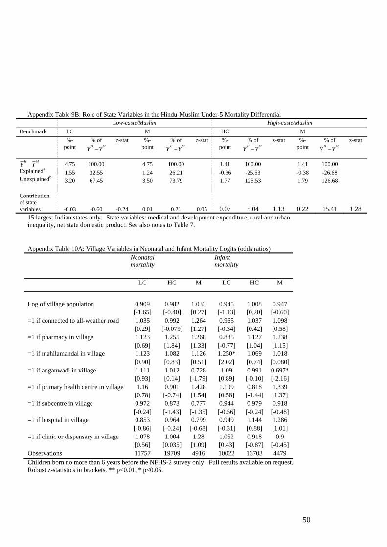
50

Appendix Table 9B: Role of State Variables in the Hindu-Muslim Under-5 Mortality Differential

Low-caste/Muslim High-caste/Muslim Benchmark LC M HC M %-

point % of H M

Y Y−

z-stat %-point

% of H M

Y Y− z-stat %-

point % of H M

Y Y− z-stat %-

point % of H M

Y Y− z-stat

H MY Y− 4.75 100.00 4.75 100.00 1.41 100.00 1.41 100.00 Explaineda

1.55 32.55 1.24 26.21 -0.36 -25.53 -0.38 -26.68 Unexplainedb

3.20 67.45 3.50 73.79 1.77 125.53 1.79 126.68 Contribution of state variables -0.03 -0.60 -0.24 0.01 0.21 0.05 0.07 5.04 1.13 0.22 15.41 1.28

15 largest Indian states only. State variables: medical and development expenditure, rural and urban inequality, net state domestic product. See also notes to Table 7. Appendix Table 10A: Village Variables in Neonatal and Infant Mortality Logits (odds ratios) Neonatal

mortality Infant

mortality

LC HC M LC HC M

Log of village population 0.909 0.982 1.033 0.945 1.008 0.947 [-1.65] [-0.40] [0.27] [-1.13] [0.20] [-0.60] =1 if connected to all-weather road 1.035 0.992 1.264 0.965 1.037 1.098 [0.29] [-0.079] [1.27] [-0.34] [0.42] [0.58] =1 if pharmacy in village 1.123 1.255 1.268 0.885 1.127 1.238 [0.69] [1.84] [1.33] [-0.77] [1.04] [1.15] =1 if mahilamandal in village 1.123 1.082 1.126 1.250* 1.069 1.018 [0.90] [0.83] [0.51] [2.02] [0.74] [0.080] =1 if anganwadi in village 1.111 1.012 0.728 1.09 0.991 0.697* [0.93] [0.14] [-1.79] [0.89] [-0.10] [-2.16] =1 if primary health centre in village 1.16 0.901 1.428 1.109 0.818 1.339 [0.78] [-0.74] [1.54] [0.58] [-1.44] [1.37] =1 if subcentre in village 0.972 0.873 0.777 0.944 0.979 0.918 [-0.24] [-1.43] [-1.35] [-0.56] [-0.24] [-0.48] =1 if hospital in village 0.853 0.964 0.799 0.949 1.144 1.286 [-0.86] [-0.24] [-0.68] [-0.31] [0.88] [1.01] =1 if clinic or dispensary in village 1.078 1.004 1.28 1.052 0.918 0.9 [0.56] [0.035] [1.09] [0.43] [-0.87] [-0.45] Observations 11757 19709 4916 10022 16703 4479 Children born no more than 6 years before the NFHS-2 survey only. Full results available on request. Robust z-statistics in brackets. ** p<0.01, * p<0.05.

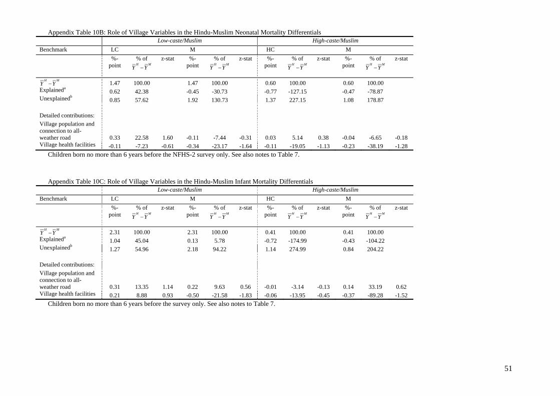
51

Appendix Table 10B: Role of Village Variables in the Hindu-Muslim Neonatal Mortality Differentials Low-caste/Muslim High-caste/Muslim Benchmark LC M HC M %-

point % of H M

Y Y−

z-stat %-point

% of H M

Y Y−

z-stat %-point

% of H M

Y Y−

z-stat %-point

% of H M

Y Y−

z-stat

H MY Y− 1.47 100.00 1.47 100.00 0.60 100.00 0.60 100.00 Explaineda

0.62 42.38 -0.45 -30.73 -0.77 -127.15 -0.47 -78.87 Unexplainedb

0.85 57.62 1.92 130.73 1.37 227.15 1.08 178.87 Detailed contributions: Village population and connection to all-weather road 0.33 22.58 1.60 -0.11 -7.44 -0.31 0.03 5.14 0.38 -0.04 -6.65 -0.18 Village health facilities -0.11 -7.23 -0.61 -0.34 -23.17 -1.64 -0.11 -19.05 -1.13 -0.23 -38.19 -1.28

Children born no more than 6 years before the NFHS-2 survey only. See also notes to Table 7.

Appendix Table 10C: Role of Village Variables in the Hindu-Muslim Infant Mortality Differentials

Low-caste/Muslim High-caste/Muslim Benchmark LC M HC M %-

point % of H M

Y Y−

z-stat %-point

% of H M

Y Y−

z-stat %-point

% of H M

Y Y−

z-stat %-point

% of H M

Y Y−

z-stat

H MY Y− 2.31 100.00 2.31 100.00 0.41 100.00 0.41 100.00 Explaineda

1.04 45.04 0.13 5.78 -0.72 -174.99 -0.43 -104.22 Unexplainedb

1.27 54.96 2.18 94.22 1.14 274.99 0.84 204.22 Detailed contributions: Village population and connection to all-weather road 0.31 13.35 1.14 0.22 9.63 0.56 -0.01 -3.14 -0.13 0.14 33.19 0.62 Village health facilities 0.21 8.88 0.93 -0.50 -21.58 -1.83 -0.06 -13.95 -0.45 -0.37 -89.28 -1.52

Children born no more than 6 years before the survey only. See also notes to Table 7.

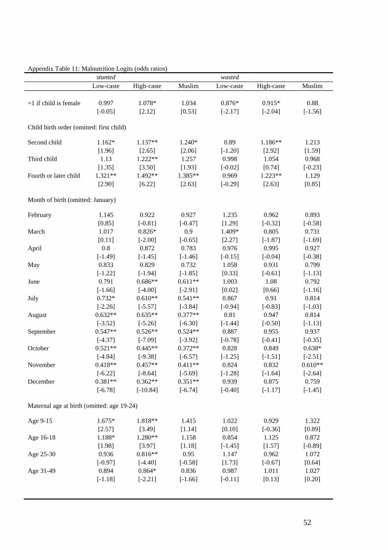
52

Appendix Table 11: Malnutrition Logits (odds ratios) stunted wasted Low-caste High-caste Muslim Low-caste High-caste Muslim =1 if child is female 0.997 1.078* 1.034 0.876* 0.915* 0.88 [-0.05] [2.12] [0.53] [-2.17] [-2.04] [-1.56] Child birth order (omitted: first child) Second child 1.162* 1.137** 1.240* 0.89 1.186** 1.213 [1.96] [2.65] [2.06] [-1.20] [2.92] [1.59] Third child 1.13 1.222** 1.257 0.998 1.054 0.968 [1.35] [3.50] [1.93] [-0.02] [0.74] [-0.23] Fourth or later child 1.321** 1.492** 1.385** 0.969 1.223** 1.129 [2.90] [6.22] [2.63] [-0.29] [2.63] [0.85] Month of birth (omitted: January) February 1.145 0.922 0.927 1.235 0.962 0.893 [0.85] [-0.81] [-0.47] [1.29] [-0.32] [-0.58] March 1.017 0.826* 0.9 1.409* 0.805 0.731 [0.11] [-2.00] [-0.65] [2.27] [-1.87] [-1.69] April 0.8 0.872 0.783 0.976 0.995 0.927 [-1.49] [-1.45] [-1.46] [-0.15] [-0.04] [-0.38] May 0.833 0.829 0.732 1.058 0.931 0.799 [-1.22] [-1.94] [-1.85] [0.33] [-0.61] [-1.13] June 0.791 0.686** 0.611** 1.003 1.08 0.792 [-1.66] [-4.00] [-2.91] [0.02] [0.66] [-1.16] July 0.732* 0.610** 0.541** 0.867 0.91 0.814 [-2.26] [-5.57] [-3.84] [-0.94] [-0.83] [-1.03] August 0.632** 0.635** 0.377** 0.81 0.947 0.814 [-3.52] [-5.26] [-6.30] [-1.44] [-0.50] [-1.13] September 0.547** 0.526** 0.524** 0.887 0.955 0.937 [-4.37] [-7.09] [-3.92] [-0.78] [-0.41] [-0.35] October 0.521** 0.445** 0.372** 0.828 0.849 0.638* [-4.84] [-9.38] [-6.57] [-1.25] [-1.51] [-2.51] November 0.418** 0.457** 0.411** 0.824 0.832 0.610** [-6.22] [-8.64] [-5.69] [-1.28] [-1.64] [-2.64] December 0.381** 0.362** 0.351** 0.939 0.875 0.759 [-6.78] [-10.84] [-6.74] [-0.40] [-1.17] [-1.45] Maternal age at birth (omitted: age 19-24) Age 9-15 1.675* 1.818** 1.415 1.022 0.929 1.322 [2.57] [3.49] [1.14] [0.10] [-0.36] [0.89] Age 16-18 1.188* 1.280** 1.158 0.854 1.125 0.872 [1.98] [3.97] [1.18] [-1.45] [1.57] [-0.89] Age 25-30 0.936 0.816** 0.95 1.147 0.962 1.072 [-0.97] [-4.40] [-0.58] [1.73] [-0.67] [0.64] Age 31-49 0.894 0.864* 0.836 0.987 1.011 1.027 [-1.18] [-2.21] [-1.66] [-0.11] [0.13] [0.20]

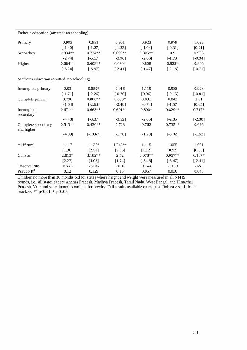
53

Father’s education (omitted: no schooling)

Primary 0.903 0.931 0.901 0.922 0.979 1.025 [-1.40] [-1.27] [-1.23] [-1.04] [-0.31] [0.21] Secondary 0.834** 0.774** 0.699** 0.805** 0.9 0.963 [-2.74] [-5.17] [-3.96] [-2.66] [-1.78] [-0.34] Higher 0.684** 0.603** 0.690* 0.808 0.823* 0.866 [-3.24] [-6.97] [-2.41] [-1.47] [-2.16] [-0.71] Mother’s education (omitted: no schooling)

Incomplete primary 0.83 0.859* 0.916 1.119 0.988 0.998 [-1.71] [-2.26] [-0.76] [0.96] [-0.15] [-0.01] Complete primary 0.798 0.806** 0.658* 0.891 0.843 1.01 [-1.64] [-2.63] [-2.48] [-0.74] [-1.57] [0.05] Incomplete secondary

0.671** 0.663** 0.691** 0.800* 0.829** 0.717*


0.513** 0.430** 0.728 0.762 0.735** 0.696

[-4.09] [-10.67] [-1.70] [-1.29] [-3.02] [-1.52] =1 if rural 1.117 1.135* 1.245** 1.115 1.055 1.071 [1.36] [2.51] [2.66] [1.12] [0.92] [0.65] Constant 2.813* 3.182** 2.52 0.078** 0.057** 0.137* [2.27] [4.03] [1.74] [-3.46] [-6.47] [-2.41] Observations 10476 25106 7610 10544 25159 7651 Pseudo R2 0.12 0.129 0.15 0.057 0.036 0.043 Children no more than 36 months old for states where height and weight were measured in all NFHS rounds, i.e., all states except Andhra Pradesh, Madhya Pradesh, Tamil Nadu, West Bengal, and Himachal Pradesh. Year and state dummies omitted for brevity. Full results available on request. Robust z statistics in brackets. ** p<0.01, * p<0.05.

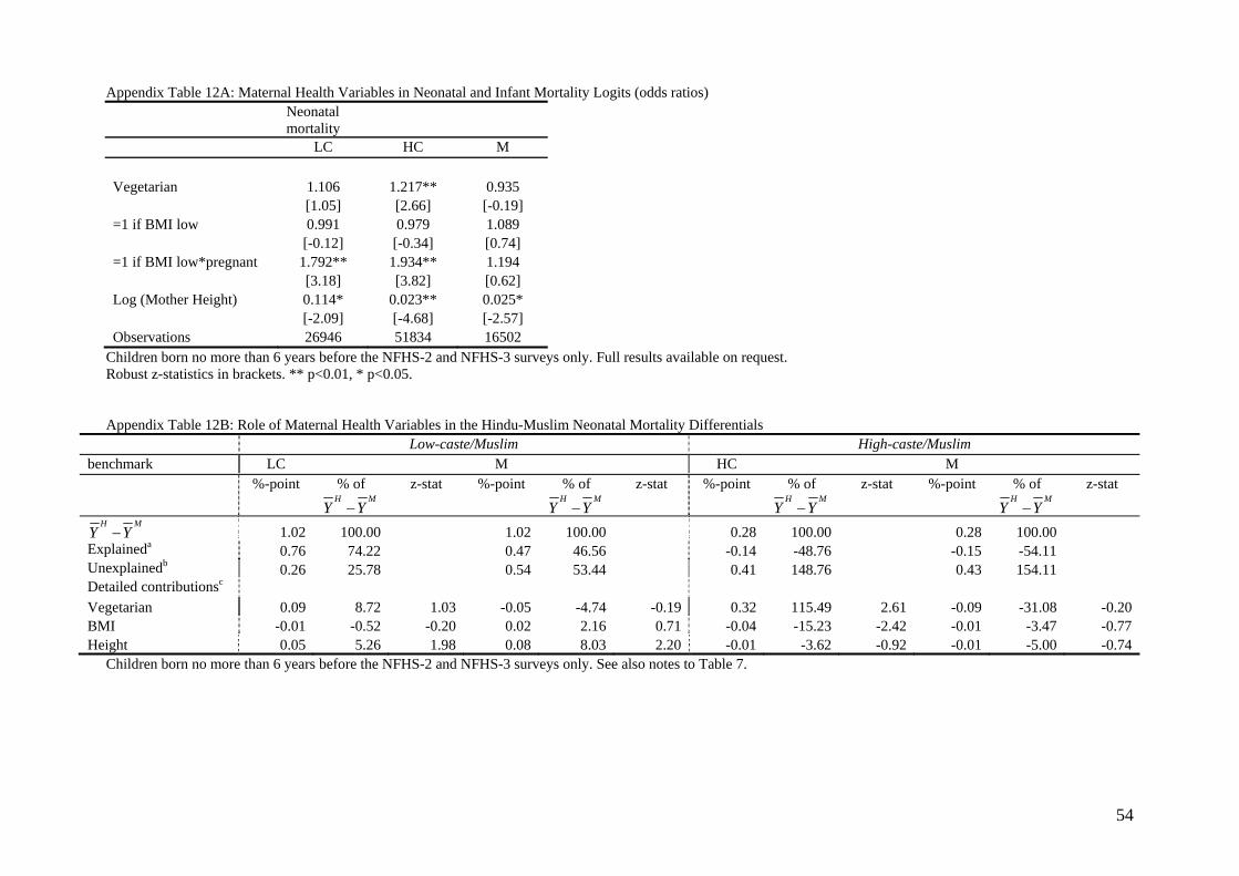
54

Appendix Table 12A: Maternal Health Variables in Neonatal and Infant Mortality Logits (odds ratios) Neonatal

mortality

LC HC M Vegetarian 1.106 1.217** 0.935 [1.05] [2.66] [-0.19] =1 if BMI low 0.991 0.979 1.089 [-0.12] [-0.34] [0.74] =1 if BMI low*pregnant 1.792** 1.934** 1.194 [3.18] [3.82] [0.62] Log (Mother Height) 0.114* 0.023** 0.025* [-2.09] [-4.68] [-2.57] Observations 26946 51834 16502

Children born no more than 6 years before the NFHS-2 and NFHS-3 surveys only. Full results available on request. Robust z-statistics in brackets. ** p<0.01, * p<0.05. Appendix Table 12B: Role of Maternal Health Variables in the Hindu-Muslim Neonatal Mortality Differentials


H MY Y−



H MY Y−


Y Y−z-stat

H MY Y− 1.02 100.00 1.02 100.00 0.28 100.00 0.28 100.00 Explaineda 0.76 74.22 0.47 46.56 -0.14 -48.76 -0.15 -54.11 Unexplainedb 0.26 25.78 0.54 53.44 0.41 148.76 0.43 154.11 Detailed contributionsc Vegetarian 0.09 8.72 1.03 -0.05 -4.74 -0.19 0.32 115.49 2.61 -0.09 -31.08 -0.20 BMI -0.01 -0.52 -0.20 0.02 2.16 0.71 -0.04 -15.23 -2.42 -0.01 -3.47 -0.77 Height 0.05 5.26 1.98 0.08 8.03 2.20 -0.01 -3.62 -0.92 -0.01 -5.00 -0.74

Children born no more than 6 years before the NFHS-2 and NFHS-3 surveys only. See also notes to Table 7.

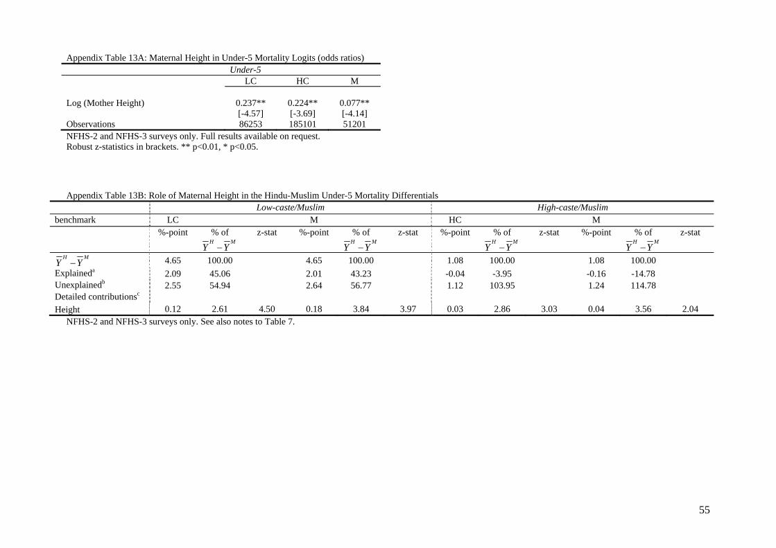
55

Appendix Table 13A: Maternal Height in Under-5 Mortality Logits (odds ratios) Under-5 LC HC M Log (Mother Height) 0.237** 0.224** 0.077** [-4.57] [-3.69] [-4.14] Observations 86253 185101 51201 NFHS-2 and NFHS-3 surveys only. Full results available on request. Robust z-statistics in brackets. ** p<0.01, * p<0.05. Appendix Table 13B: Role of Maternal Height in the Hindu-Muslim Under-5 Mortality Differentials


H MY Y−



H MY Y−


Y Y−z-stat

H MY Y− 4.65 100.00 4.65 100.00 1.08 100.00 1.08 100.00 Explaineda 2.09 45.06 2.01 43.23 -0.04 -3.95 -0.16 -14.78 Unexplainedb 2.55 54.94 2.64 56.77 1.12 103.95 1.24 114.78 Detailed contributionsc Height 0.12 2.61 4.50 0.18 3.84 3.97 0.03 2.86 3.03 0.04 3.56 2.04

NFHS-2 and NFHS-3 surveys only. See also notes to Table 7.

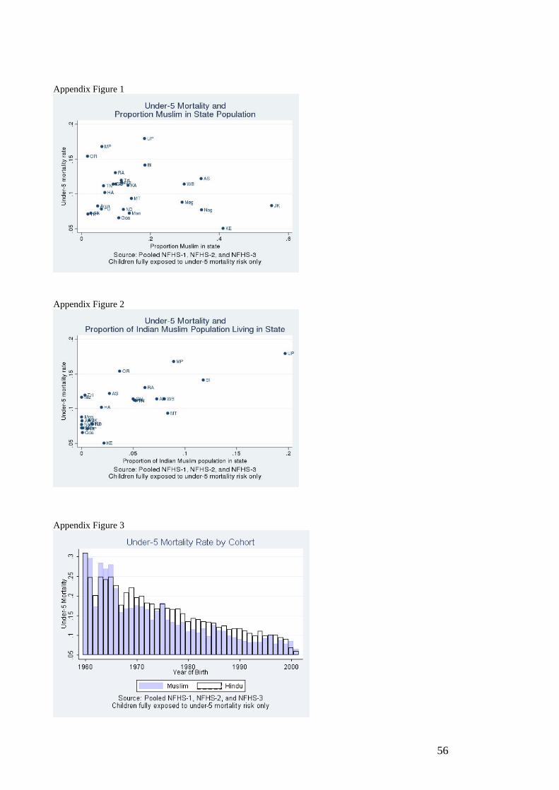
56

Appendix Figure 1

Appendix Figure 2

Appendix Figure 3

Documents

The Puzzle of Muslim Advantage in Child Survival in India - Iza