Embed Size (px)
Citation preview
Prepared for: Unum Group 2211 Congress Street Portland, ME 04122
Financial Security for Working Americans: An Economic Analysis of Insurance Products in Workplace Benefits Programs
Prepared by: Charles River Associates John Hancock Tower 200 Clarendon Street, T-33 Boston, MA 02116 Date: July 2011
Financial Security for Working Americans: An Economic Analysis of Insurance Products in Workplace Benefits Programs
Authors and contributors
This study was produced under the direction of David F. Babbel, Emeritus Professor at The Wharton School, the University of Pennsylvania and Senior Advisor and Leader of the Insurance Economics Practice at Charles River Associates. Professor Babbel was assisted in this report by Dr. Jaime Cuevas Dermody (Principal, Financial Engineering LLC of Delray Beach, Florida), Dr. Miguel Herce (Principal, Charles River Associates), Dr. Mark Meyer (Vice President and Co-Leader of the Insurance Economics Practice at Charles River Associates), and Dr. Navendu Vasavada (Financial Engineering LLC). Mr. David Schramm (Consulting Associate, Charles River Associates) and Mr. Daniel Mower (Associate, Charles River Associates) assisted in the research and production of this study.
Acknowledgements
The authors of this study want to thank Unum Group for financial support and information, particularly Scott Maker (Senior Vice President and Chief Government Affairs Officer), Tim Smith (Vice President, Government Affairs), Matt Monaghan (Vice President, Government Affairs), and Tom Hinrichs, FSA, MAAA (AVP & Actuary, Group Disability Pricing). We are also grateful for discussions with and information provided by Robert W. Beal, FSA, MAAA (Consulting Actuary, Milliman, Inc.) and Rick Leavitt (VP, Pricing and Consulting Actuary, Smith Group).
Disclaimer
The conclusions set forth herein are based on independent research and publicly available material. The views expressed herein are the views and opinions of the authors and do not reflect or represent the views of Charles River Associates or any of the organizations with which the authors are affiliated. Any opinion expressed herein shall not amount to any form of guarantee that the authors or Charles River Associates has determined or predicted future events or circumstances and no such reliance may be inferred or implied. The authors and Charles River Associates accept no duty of care or liability of any kind whatsoever to any party, and no responsibility for damages, if any, suffered by any party as a result of decisions made, or not made, or actions taken, or not taken, based on this study. Detailed information about Charles River Associates, a registered trade name of CRA International, Inc., is available at www.crai.com.
Copyright 2011 Unum Group

Financial Security for Working Americans: An Economic Analysis of Insurance Products in Workplace Benefits Programs
Charles River Associates | i
Table of contents
1. Executive summary .............................................................................................. 1
2. Impetus for the study of disability insurance ........................................................... 5
3. Introduction to the value of insurance products offered through the workplace ......... 9
4. The value of employer-sponsored insurance products to employees ....................... 14
4.1 Introduction ..................................................................................................... 14
4.2 The “premium” approach—a lower bound on value ......................................... 14
4.3 A single-period model of the value of insurance incorporating risk aversion ..... 15
4.4 The value of group disability insurance ............................................................. 18
4.5 The value of life insurance ................................................................................ 24
4.6 The value of long-term care insurance .............................................................. 27
4.7 The general multi-period model........................................................................ 28
5. The benefits of employer-supplied disability insurance to government and the taxpayer ............................................................................................... 29
5.1 Introduction ........................................................................................................ 29
5.2 Taxpayer-funded benefits in the case of disability ............................................... 30
5.3 Sizing the issue—employment, income, and assets affecting ESDI and public welfare disability insurance ....................................................................... 33
5.4 The probability of impoverishment arising from disability ................................... 36
5.5 First estimates of the short-term benefits of ESDI—easing the burden on public assistance programs.................................................................................. 38
5.6 Possible, but not-yet-quantifiable, long-term benefits of ESDI—preserving income and wealth of the newly disabled yielding more tax revenue .................. 40
5.7 The capital market benefits of employer-sponsored insurance ............................ 41
6. Conclusion ........................................................................................................ 42
Appendix A: One-period model of the welfare value of private insurance………………………….44
Appendix B: Multi-period model of long-term disability insurance……………………………………..52
Financial Security for Working Americans: An Economic Analysis of Insurance Products in Workplace Benefits Programs
Charles River Associates | ii
Tables
Table 1: US SSDI average replacement rates (2010) ................................................................. 19
Table 2: SSDI and ESDI replacement rates ............................................................................... 21
Table 3: Economic welfare value of ESDI (expense factor is 10%) ............................................. 22
Table 4: Economic welfare value of ESDI (expense factor is 15%) ............................................. 24
Table 5: Economic welfare value of ESDI (expense factor is 30%) ............................................. 24
Table 6: Economic welfare value of group life insurance (expense factor is 10% and savings ratio is 10%) ..................................................... 26
Table 7: Economic welfare value of group life insurance (expense factor is 15% and savings ratio is 10%) ..................................................... 26
Table 8: Economic welfare value of group life insurance (expense factor is 10% and savings ratio is 20%) ..................................................... 27
Table 9: Economic welfare value of group life insurance (expense factor is 15% and savings ratio is 20%) ..................................................... 27
Table 10: Characteristics of income, assets, and debt by income quintile (2007) ........................ 34
Table 11: Characteristics of income, assets, and debt by net worth quartile (2007) .................... 35
Table 12: Characteristics of income, assets, and debt by age cohort (2007) .............................. 36
Figures
Figure 1: The welfare value of insurance ................................................................................... 17
Figure 2: Optimal insurance ....................................................................................................... 46
Figure 3: Optimal insurance and the certainty line ...................................................................... 48
Figure 4: Certainty equivalents and welfare value of private insurance ....................................... 50

Financial Security for Working Americans: An Economic Analysis of Insurance Products in Workplace Benefits Programs
Charles River Associates | 1
1. Executive summary
A fundamental truth of life is that anyone, at any time, can be affected by death, disabling injury, or debilitating illness. Death during an individual’s working years can leave a family without the economic resources to meet needs and fulfill dreams. Disability during the working years means an individual suffers not only from the malady but risks losing the ability to earn a living.
These events can mean physical, emotional, and financial stress on family and friends. They can also lead one to rely on society’s resources through public assistance programs. Individuals can, and often do, arrange to lessen the financial burdens of death or disability. Governments and not-for-profit organizations have also instituted programs to alleviate economic distress. And in the modern American economy, employers facilitate and provide the means for their employees to deal with death, sickness, injury, and advancing age.
This study presents an analysis of the economic value of certain insurance products offered through workplace benefits programs in the US.
A valuable safety net
Employer-sponsored disability, life, long-term care, and critical illness insurance provide a crucial financial safety net for employees, their families, taxpayers, and society. These insurance benefits allow employees and their families to maintain a higher standard of living and financial security in the event of disability or death than if the employee and family had to rely on their savings or on government assistance. This financial security delivers significant economic value to the employee and family. Because these employer-sponsored benefits provide income in the event of a misfortune, they also prevent affected families from becoming impoverished, saving the government billions of dollars each year in public welfare program benefits.
What is the value of the employer-sponsored private insurance coverage to individuals, employers, and the government? In this study we apply rigorous economic analysis incorporating fundamental principles of consumer choice in the face of uncertainty, employer responses to tax and labor market conditions, and the provisions of government public assistance programs to answer these questions.
The value of insurance to any employee depends on the individual’s dislike of risk, but assuming typical levels of risk aversion this study demonstrates that the value of these employer-sponsored insurance products is multiples of the premiums, even if the employee never files a claim. We find, for example, that employees value each dollar of disability insurance at 20 to 60 times its cost in premiums. Similarly, employees value each dollar of life insurance at 60 to 170 times its cost in premiums. And this is looking at the value prospectively—before the employee actually receives any insured benefits. If the insurance is needed, the actual value of the benefit received is even higher for the affected employee.
Employees and their families benefit from the financial protection the insurance provides. Employers benefit from offering insurance products that help attract and retain quality workers. Society benefits from the economic safety net these products supply, and the government avoids billions of dollars in public assistance payments as a direct consequence of the insurance.
Financial Security for Working Americans: An Economic Analysis of Insurance Products in Workplace Benefits Programs
Charles River Associates | 2
An affordable resource
Premiums on group disability and life insurance available through employers are generally quite low.
Group disability premiums can be as little as $25 per month or $300 per year.
Group term life insurance premiums for someone just starting a career can be less than $1 per year per $1,000 of death benefit.
Other group insurance products benefit similarly from the economics of group underwriting. In return for the modest sum of about $300 per year, covered employees receive significant benefits.
An employee in his thirties can obtain a $300,000 group term life policy.
An employee in his forties earning $80,000 to $85,000 per year experiencing a disability can obtain approximately $1 million over 20 years from an employer-sponsored disability plan.
An employee in his twenties earning $40,000 to $50,000 per year suffering a disability can obtain well over $1 million in payments from an employer-sponsored disability plan.
Adding up the benefits
This study goes beyond the concrete but limited examples above to rigorously quantify the economic welfare value of employer-sponsored disability and group life insurance. For an individual starting a 40-year or longer career at $50,000 per year in salary, the economic welfare value of employer-sponsored disability insurance over the span of the anticipated career is at least $500,000.
In other words, an individual at the start of his working career informed of the probability of a disabling injury or sickness and the stream of benefit payments arising from the employer-sponsored disability insurance would value the disability coverage at a minimum of $500,000.
If the individual is more than moderately risk-averse, the value of the disability insurance would be higher—perhaps $1 million or more. This is the present economic welfare value of employer-sponsored disability insurance for one individual circumstance.
This study finds that the total economic welfare value for all employees covered by employer-sponsored disability insurance (approximately 40 million employees) is between $230 billion and $590 billion. Total premiums for employer-sponsored disability insurance are approximately $10 billion annually. The ratio of economic value for the employee to premium cost is clearly large—for each dollar of premiums paid, employees obtain an economic welfare value of between $20 and $60.
Using the same analytical approach, we find that the total economic welfare value for all individuals covered by employer-sponsored group life insurance (approximately 75 million employees and 105 million lives) is between $1.25 trillion and $3.58 trillion annually. Total premiums for employer-sponsored group life insurance are approximately $21 billion annually Again, the ratio of economic value for the employee to premium cost is large—for each dollar of premiums paid, employees obtain an economic welfare value between $60 and $170.
Financial Security for Working Americans: An Economic Analysis of Insurance Products in Workplace Benefits Programs
Charles River Associates | 3
It is important to recognize that these large economic welfare values for group disability and group life insurance arise from only a fraction of the US working population. In 2009, only 60% of civilian wage earners were covered by group life insurance, and only 32% were covered by group long-term disability insurance.1
The total economic welfare value of these insurance products could be substantially higher if more employers would make the insurance available to their workers, especially in the lower and middle wage levels where access to group insurance products is comparatively lower than at higher wage levels.2
Offering broad social value
In addition to the economic welfare value that employees individually and as a group attribute to employer-sponsored insurance benefits, these same products provide undeniable and concrete benefits to the government and the taxpayers.
The existence of employer-sponsored insurance products decreases the dependency on public assistance programs and increases public revenues by providing a stream of income that prevents families from falling into distressed financial straits.
This study documents that the income protection provided by employer-sponsored disability insurance alone means that between 280,000 and 575,000 families each year avoid impoverishment and, therefore, do not need public assistance programs. This is because approximately three-fourths of those disabled receiving employer-sponsored disability insurance would, in its absence, become impoverished and have to rely on public assistance programs.
On a very conservative basis, this translates into a savings to the government (and the taxpayer) of at least $2.25 to $4.5 billion per year. So, in addition to the pure economic welfare value of group disability insurance to the individuals, it actually saves significant public resources at the same time.
The analysis conducted in this study demonstrates that employer-sponsored insurance products provide enormous value to employees, employers, and the government. A crucial component of this value is how employer-sponsored insurance works with government programs and individually provided resources in a manner that benefits all parties—the employees, employers, and the government.
1 US Bureau of Labor Statistics, National Compensation Survey: Employee Benefits in the United States, March 2009, Bulletin 2731, Table 16. The same participation rate for group life insurance, 60%, was also reported by the Bureau in 2010, although they did not report the participation rate for group disability insurance in this publication. See US Bureau of Labor Statistics, Employee Benefits in the United States—March 2010, USDL-10-1044, July 27, 2010, Table 5, p. 13.
2 The “take-up rates” for group life and disability insurance is very high across all wage percentiles—starting in the high 80s for the lowest 10% of civilian wage earnings and rising to the 90s for the higher civilian wage earners. “Access” to these insurance benefits, however, rises notably with wages. This pattern indicates that employers with higher-earning workforces provide more access to these insurance workplace benefits. Access also increases with increasing firm size as measured by number of employees. US Bureau of Labor Statistics, National Compensation Survey: Employee Benefits in the United States, March 2009, Bulletin 2731, Table 16.
Financial Security for Working Americans: An Economic Analysis of Insurance Products in Workplace Benefits Programs
Charles River Associates | 4
Of particular note is the way the widely available but limited benefits of the government disability insurance program integrates with the more expansive benefits of the private program to generate substantial societal support for the government program while simultaneously allowing for individual choice. In light of increasingly burdened public welfare systems such as the Social Security Disability Insurance (SSDI) program, this study documents that robust private sector insurance products can and do play a critical role in ensuring adequate financial security for working Americans.

Financial Security for Working Americans: An Economic Analysis of Insurance Products in Workplace Benefits Programs
Charles River Associates | 5
2. Impetus for the study of disability insurance
If you were asked what your most valuable possession is, how would you respond? Homeowners might say it is their house (although these days, due to the recent financial crisis, for many of us our homes are worth less than is owed).
In any given year there are roughly three chances in 1,000 that our houses and their contents will be damaged by fire, although the chances of fire leading to a total loss are much lower. Of course, depending on location, we could also lose or have our houses and their contents damaged in a mudslide, windstorm, or other calamity. Most of us have insurance against such losses.
Younger people or renters might say their most valuable possession is their automobile. It may be worth thousands of dollars, net of any remaining auto loan. During any single year, there is approximately one chance in 100 that an automobile will be stolen and, over our lifetimes, a one in four chance that we will be involved in an automobile accident, according to the National Safety Council. Our chances of dying in a car crash over a lifetime are about 1%.3 The odds for a given individual depend on a lot of factors, such as type of car, gender, age, location, driving habits, miles driven, and so forth. Most of us have auto insurance coverage against these contingencies.
If a good economist were asked the same question, she would likely respond that for most people in the workforce—all but those nearing retirement—the most valuable asset is their “human capital” (i.e., their ability to earn a wage or salary or to obtain income from their own business). Consider for a moment the value of human capital. In the US, a typical level of annual income for an individual worker is somewhat less than $50,000. People at the start of their careers often earn less while those with more experience and education may earn more—some substantially more. Using the $50,000 figure as a standard, a person over his or his working life of (say) 44 years may have earned upwards of $2.2 million.
So, what are the odds of losing part or all of that potential income due to disability? Perhaps surprisingly, about one in three workers will be disabled for at least six months during the course of his or her earning years, according to the Social Security Administration. The median length of the disability is two-and-a-half years, although half of the time it is longer—sometimes much longer, such as 30 or more years. Failing to protect the very valuable asset of human capital exposes the individual and his or her dependents to a high risk with a probability of loss akin to that faced when playing Russian roulette with a three-shooter with only two empty chambers. Few Americans are willing to play such a risky game with assets such as their home or car, yet many leave their most valuable asset exposed to tremendous risk. Financially speaking, the risk is higher than that of three-shooter roulette because when a worker becomes disabled, the costs of sustaining that individual’s life do not go away but continue to drain household resources.
How can we protect ourselves against that financial risk? The first recourse is typically a reliance on personal savings. There are two problems with this solution. First, 71% of American
3 National Safety Council, Injury Facts, 2008 Edition.

Financial Security for Working Americans: An Economic Analysis of Insurance Products in Workplace Benefits Programs
Charles River Associates | 6
households consume 100% or more (through credit cards and debt) of their paycheck each month.4 This leaves nothing for savings. Of course, we might be able to net something from our car or the sale of other household possessions at the local pawn shop or on Craigslist, but we’ll probably run out of cash unless our disability lasts only for a very short time.
Second, if we find ourselves among the 29% of American households who do save money each month, we’ll be able to handle a few more months—or perhaps years, depending on how soon in our working life the disability occurs—of disability. But if the disability hits before we’re 45, we’re potentially leaving more than $1 million on the table, and it takes time to accumulate that much in personal savings. Sure, we could tap our retirement account if we have one, but then what will be left for retirement—a period that typically lasts for 20 years and can exceed 30 years?
The next recourse we may have is our family. If married, perhaps we could get by on one income if we scale down our expenses and sufficiently reduce our lifestyle. However, the lives of many families already lack enough “extras” to reduce it by much. If that is not a viable option, we could become dependent on public or private welfare. Perhaps we may need to go beyond our spouse and include our extended family before we find sufficient resources to help. Unfortunately, these days families and even extended families are often overextended and can offer no help, but family can offer some assistance in many cases.
If our disability was occasioned by work-related activities, we may be eligible for workers’ compensation. This is a program that will cover injury-related medical expenses and provide a monthly income for some percentage of lost wages. The income replacement can be as high as two-thirds of normal pay up to some limit (such as state average weekly wages), depending on where we reside. In addition to limitations on the percentage of pay replaced, workers’ compensation programs are also limited in duration with maximum benefit payment periods of 200 to 400 weeks.5
More crucially, 90% of disabilities are not caused by work-related injuries or conditions6 and are therefore not covered by workers’ compensation programs. The most common causes of long-term disability are cancer, complications of pregnancy, back injuries, stroke and neurological disease, and other injuries.
The next layer of financial protection, and for many of us the first and only layer, is public assistance of some sort. Thankfully, in the US, we do have some limited coverage for disability as part of the federal Social Security Disability Insurance (SSDI) program. To be eligible, we must prove that we have a total disability that will last longer than one year. For various reasons, most disabilities do not qualify under this standard. Approximately 70% of first-time applicants for benefits under this federal program are denied. What then?
4 American Payroll Association, “Getting Paid in America” Survey, 2008.
5 See US Chamber of Commerce, Analysis of Workers’ Compensation, 2008 (and updates); The Workers’ Compensation Compendium, Workers’ Disability Income Systems, Inc., Princeton, NJ, 2006; and State Workers’ Compensation Laws, Office of Workers’ Compensation Programs, Employment Standards Administration, US Department of Labor, 2005.
6 National Safety Council, Injury Facts, 2008 edition.
Financial Security for Working Americans: An Economic Analysis of Insurance Products in Workplace Benefits Programs
Charles River Associates | 7
If we do wind up qualifying for SSDI benefits, it typically takes about two years before we receive our first payment. With the loss of income, how do we cover our expenses during the interim? If we are denied Social Security disability benefits upon first application, as most applicants are, we can appeal—indeed, there are four layers of appeal. The typical waiting period is longer than 880 days,7 and the appeals process can be costly as well as unsuccessful. What then? Even if we are ultimately awarded benefits, it is likely that our lives will suffer major disruption while waiting for the administrative process to conclude. (We note that in 2005, one study claimed that about half of all home foreclosures were precipitated by a disability—and this was before the massive parade of foreclosures occasioned by the Great Recession of 2007–2009.8 This is a telling indicator of the nature of disruption people suffer when a disability strikes a household.)
If we are judged eligible for benefits under the SSDI program, we will eventually be paid a portion of our salary/wages, and the larger the salary/wages the smaller the portion. Although the SSDI taxes collected are a fixed proportion of income up to the taxable maximum, the program payouts are structured in a manner that provides a declining proportion of the pre-disability income—i.e., the program favors most those who were earning the least. For example, if we were earning $17,000 per year, we will receive 59% of our prior annual earnings in the event of disability. If we were earning $37,000 annually, we will receive 43% of our prior earnings, and if our former earnings were $106,800, we will receive only about 22%. Any earnings levels above $106,800 will receive no more in absolute dollars, translating into an ever-decreasing percentage of pre-disability income coverage. People who are in any one but the lowest earnings echelon will most likely have to drastically alter their living standard should they become disabled and have to rely on only SSDI benefits.
Fortunately, private disability insurance is available to supplement SSDI and other public benefit programs. Many of us are eligible to participate in our companies’ group disability programs. In such programs, we are typically covered for short-term disabilities lasting one to six months but can elect to obtain or are automatically covered for long-term disability coverage as well. This coverage may cost as little as $300 per year per employee. If we work for an employer that does not offer this benefit, we can buy it directly as an individual, although in most cases premiums are higher for an individual policy.
Unlike the public program, which offers decent coverage if we’re in the lowest 10% of the income distribution (60% of lost wages) but much lower coverage if we have higher income to cover (perhaps less than 10%), with private disability insurance we can supplement federal coverage so that our total coverage can reach 60% or more of lost income.
One of the valuable aspects of private disability insurance is that benefit payments can start immediately through the short-term disability program and then continue uninterrupted through the long-term disability program. Then, if and when SSDI begins paying disability benefits, the
7 See SSDI Fast Facts and Figures, 2010.
8 See Health Affairs, Policy Journal of the Health Sphere, February 2, 2005. The same study shows that only 2% of home foreclosures are caused by death, so disability creates a much higher risk of losing one’s home.
Financial Security for Working Americans: An Economic Analysis of Insurance Products in Workplace Benefits Programs
Charles River Associates | 8
private insurance benefits may be reduced to maintain the overall level of disability benefit chosen and purchased: for example, 60% of salary.9
The existence of private disability insurance is particularly important for those people deciding to invest eight to 12 years in higher education, incurring upwards of $300,000 in additional schooling costs, and foregoing the earnings that could have been received over those years had they chosen to enter the workforce. Consider a medical student or PhD scientist. A disability could end their ability to earn a living and their ability to repay their heavy debt burden from investing in the additional "human capital" it takes to perform these occupations. Although this group may be a relatively small portion of the population, it is a key segment and it is important to society to encourage these investments in time and money for the benefit of us all. Without the availability of disability insurance, such an educational and training undertaking could be financially reckless.
Many types of insurance from various sources (private companies, public agencies, and one’s own savings as self-insurance) provide a wide variety of protection from the negative events that occur in our lives. An important, but in our opinion understudied, source of insurance protection are those programs supplied, supported, or facilitated by employers for the benefit of their employees. Now that we have outlined the protections that one of these employer-sponsored insurance programs offers to employees, we will devote the remainder of this study to understanding and quantifying where possible the value of some of these programs to the employee, the employer, and the government.
9 An important factor in the affordability of disability insurance is its integration with government disability insurance programs such as Social Security Disability Insurance. The integration has a double benefit. To the extent that government program payments replace private insurance payments, the cost for the private insurance is lower. The private insurance also allows employees to replace a significantly higher portion of their pre-disability income and generally initiates payments far more quickly than the government program. These advantages benefit the disabled individual enormously while also reducing the call on public assistance programs.

Financial Security for Working Americans: An Economic Analysis of Insurance Products in Workplace Benefits Programs
Charles River Associates | 9
3. Introduction to the value of insurance products offered through the workplace
In the US, individuals can obtain protection from adverse events, such as a disability, via several means.
First, an individual can make his own arrangements by accumulating savings or purchasing an insurance policy. While this path is common for protecting against certain types of adverse events (e.g., auto insurance, homeowners’ or renters’ insurance, life insurance, individually purchased disability insurance, etc.) and involves some interesting analysis, individually purchased insurance is not the focus of this investigation.
Second, society as a whole, as represented by government at various levels, can also provide protection or compensation to individuals as part of a social insurance program. Some of these are mandatory programs at least partially financed by dedicated taxes (e.g., Social Security and Medicare) or means-tested programs mostly financed from general tax revenues (public assistance programs such as Medicaid, Temporary Assistance to Needy Families, Supplemental Nutrition Assistance, or other programs). The rationale for government involvement in designing and implementing these social insurance programs is largely twofold: (1) by mandatory participation, the government can mitigate adverse selection issues; and (2) the programs can be designed to redistribute income or wealth to the more needy. In the US, all levels of government can have some role in designing or implementing at least some elements of the “social safety net,” as some have called it.
The health care and Social Security systems in the US, for example, are fundamental components of the social safety net that advanced industrial societies have developed to protect individuals against the economic consequences of illness and disability as well as to provide retirement and unemployment income. In spite of their success and wide acceptability, the medium- and long-term sustainability of the health care and Social Security systems at their current levels, in the US as well as in most advanced economies, has been questioned. These government programs face notable challenges that include rising medical costs, unfavorable demographic and employment trends, increasing life expectancies, increasing disability morbidity, and the weight of mounting public debt. Recent legislative efforts and proposals in the US and numerous reports by public interest groups and academics point to an urgent need to substantially reform the current health care and Social Security programs. This reform, should it happen, will be a complex and contentious process, but we think it accurate to say that the role of the private insurance sector will continue, and should be enhanced, given the grim outlook for public finances and the hard choices that will need to be made in the years ahead. Indeed, it can be reasonably concluded that by expanding the role of private insurance in the areas of health, life, disability, and retirement income, more efficient health care and Social Security programs will be able to preserve their position as an important element of social policy.10 While these
10 The Social Security tax rate in the US is currently a fixed percentage of gross wages up to a maximum Social Security Wage Base. Although this tax formula is regressive, the benefits formula used is progressive in the sense that the percentage of earnings replaced by retirement pensions and disability benefits is significantly higher for lower-earning
Financial Security for Working Americans: An Economic Analysis of Insurance Products in Workplace Benefits Programs
Charles River Associates | 10
government programs are large, ubiquitous, and the subject of much study and debate, their design and use are not the primary focus of this investigation.11
The third method by which individuals can obtain protection is through their employers. Most people in the US, for example, currently obtain their health insurance coverage through the auspices of their employers.12 Many employers also provide the means through which their employees obtain some level of retirement income (defined benefit or defined contribution pension programs).13 And, the focus of this investigation, employers also sponsor or facilitate the ability of their employees to obtain disability insurance (short- and long-term), life insurance, supplemental insurance, and long-term care insurance.
In the US, the two main insurance products among the ones we focus on in this report—group life insurance and group disability insurance—cover large segments of the private sector labor force. In 2009, the group life insurance industry had policies in force covering approximately 105 million employees (about two-thirds of the private sector labor force) with annual premiums of more than $21 billion and associated face value of in-force insurance of approximately $7.25 trillion. Also, for 2009, the group long-term disability insurance industry had policies in force covering approximately 40 million employees with annual premiums of about $9.8 billion.14 These figures attest to the significant usage in the US of the employer-sponsored insurance products we consider.
Why do employers expend the resources to provide, sponsor, or facilitate various types of insurance for their employees? In the first place, employer-provided insurance is part of each employee’s total compensation package. Economists studying labor decisions have long recognized that employees evaluate not only the salary or wage they will earn at a particular employer, but also many other elements that determine the employees’ satisfaction with the job—the work environment, the length of the commute, the content of the job, the prospects for advancement, the amount of vacation, etc. Additional benefits, such as employer-provided
individuals than it is for middle- and, especially, higher-earning individuals. This implies that higher-earning individuals effectively subsidize the pensions of lower-earning individuals. The progressiveness of the benefits formula is one example of the social policy aspect of social security to which we refer. Other notable examples can be found in Medicare and Medicaid.
11 The way these programs interact with employer-sponsored disability insurance, the focus of this study, will be addressed in later analysis.
12 Fifty-five percent of all civilian workers participate in medical care benefit programs through their employer. Restricting attention only to full-time employees, 67% participate in medical care benefit programs through their employer. As wages increase, the participation rate also increases. US Bureau of Labor Statistics, Employee Benefits in the United States—March 2010, USDL-10-1044, July 27, 2010, Table 2, p. 7.
13 Fifty-five percent of all civilian workers participate in retirement benefit programs through their employer. Restricting attention only to full-time employees, 65% participate in retirement benefit programs through their employer. As wages increase, the participation rate also increases. Ibid., Table 1, p. 5.
14 JHA: 2009 US Group Life Market Survey; 2009 US Group Disability Market Survey Summary Report. Lives covered by group life insurance are from “2011 Group Disability & Group Life Insurers,” accessed May 25, 2011, http://www.workforce.com/section/benefits-compensation/feature/2010-group-disability-group-life-insurers/index.html. Approximately two million people obtain disability insurance through individual policies.

Financial Security for Working Americans: An Economic Analysis of Insurance Products in Workplace Benefits Programs
Charles River Associates | 11
insurance, are part of the total compensation package that each employee (or potential employee) considers.15 Surveys demonstrate that insurance products available through the workplace can be part of that evaluation. Almost half of employees in a recent survey cited employee benefits as “an important reason why I came to work for this company.” And 60% of the surveyed employees agreed that “the employee benefits offered to me are an important reason why I remain with my employer.” This same survey found that “employees who are satisfied with benefits are more likely to be loyal and satisfied with their jobs” and “employees who are satisfied with benefits are least likely to leave and believe that benefits are an important reason to stay.”16
Another important motivator for employers to provide certain types of insurance coverage is government taxation and regulation. Governments at all levels and around the world have decided that employers must provide certain types of either governmentally or privately supplied insurance programs—Social Security, Medicare, unemployment insurance, workers’ compensation insurance, etc. Governments have also decided that certain other types of insurance are so beneficial to society that they have endowed these programs with beneficial tax treatment. In the US, for example, health insurance paid for by employers is deductible from their income, whereas an individual cannot deduct health insurance premiums on his or her tax return. Certain types of retirement income programs, which can be considered a type of insurance, are tax-favored in that employers’ contributions to defined benefit programs and any matching amounts they provide to their employees’ defined contribution programs are tax-deductible. This tax deductibility at the employer level influences the mix of types of compensation provided to employees. Those programs that are tax favored are generally more prevalent as “fringe benefits” in employees’ compensation programs.
Employers, however, also sponsor or facilitate other types of privately supplied insurance products for their employees—and those products are the focus of this investigation. In 2009, according to the US Bureau of Labor Statistics, 62% of all civilian workers had access to life insurance through their employer, and 96% of those who had access obtained it. Similarly, 37% of all civilian workers had access to a short-term disability program, and 33% had access to a long-term disability program through their employers. The “take rate” for these was similarly high—97% and 96%, respectively. If you limit attention to those civilian workers with full-time jobs, employee access increases (and the “take rate” is no lower): 76% access for life insurance, 44% for short-term disability, and 41% for long-term disability.17 In the case of these three products, the tax situation is somewhat complicated. At least a portion of the cost of providing these can be tax favored, although employees are likely better off paying for the disability coverage (especially long-term) out of after-tax dollars.18
15 See, for example, Campbell McConnell, Stanley Brue, and David Macpherson, Contemporary Labor Economics (2009), Chapter 7.
16 MetLife, 9th Annual Study of Employee Benefits Trends: A Blueprint for the New Benefits Economy, 2011, pp. 15–6.
17 US Bureau of Labor Statistics, National Compensation Survey: Employee Benefits in the United States, March 2009, Bulletin 2731, Table 16. The figures for life insurance are confirmed in the available 2010 data. See US Bureau of Labor Statistics, Employee Benefits in the United States—March 2010, USDL-10-1044, July 27, 2010, Table 5, p. 13.
18 Generally speaking, the premiums for employer-provided group term life insurance are tax-deductible to the employer up to a certain level of coverage—currently $50,000. Any premiums for coverage over that amount are, under most typical
Financial Security for Working Americans: An Economic Analysis of Insurance Products in Workplace Benefits Programs
Charles River Associates | 12
With less compelling tax benefits for the provision of life and disability insurance, why would an individual employee choose to obtain life and disability insurance through their employer rather than purchase these directly as an individual? One reason is that employers can facilitate the coverage on a group basis. This has two advantages for the employee. First, there is little or no underwriting or examination of the individual to determine his or her insurability. This makes it extremely convenient for the employee to obtain coverage. There is no visit to an insurance agent and no medical examination involved. At the same time the employee is making a decision on other benefits offered by the employer, he or she can quickly and easily sign up for meaningful amounts of group life, group disability, critical illness, and long-term care insurance coverage. The convenience factor is significant, and there is no insurance agent selling other products you may not yet need.
The second advantage is that group coverage tends to be less expensive because there are cost and underwriting efficiencies in the process that do not always apply to the sale of individual disability insurance in a one-to-one setting. Obtaining individual coverage often involves a selling agent that obtains some level of compensation for his or her efforts. Individual coverage is also subject to a potentially higher level of “adverse selection”— a greater likelihood that less healthy or more accident-prone people would seek out individual coverage. Through group coverage, the insurer, in a sense, uses the employer’s screening process for hiring as a means to avoid excessive adverse selection. Group coverage also means that the selling compensation and other necessary distribution and setup cost per policy is lower than when it is done on an individual basis. At least these two factors lower the costs of insuring employees through group coverage as opposed to each employee obtaining individual coverage.
The fact that employers sponsor various forms of group insurance extends the opportunity for such coverage to individuals and families that otherwise might find access to insurance restricted by cost or lack of information. For many people starting out in their careers, employer-sponsored insurance programs are their first encounter with the realities of financial risk and planning. For some who are older, actively seeking insurance may prove difficult with the other demands of their lives. This facilitated access in a controlled environment is conducive to thoughtful decisions.
Can the employer accrue any benefits from facilitating group insurance purchases by its employees? As an initial matter, recall that employees consider many factors when determining whether to take, or stay at, a particular job. The level of fringe benefits, including the availability and cost of group life and disability insurance, will enter into many employees’ considerations. And competition for the best workforce will make the absence of such coverage, holding all else equal, a disadvantage to employers.19
In addition, disability insurers in particular have economic incentives and notable capabilities to minimize the cost of disabilities to themselves, employees, and employers. Each employee who
circumstances, taxable income for the employee. Tax-deductible disability premiums generally result in taxable benefit payments should disability occur. Paying disability premiums with after-tax dollars generally results in non-taxable benefit payments should disability occur. For many (if not most) employees, the expected advantage of non-taxable benefit payments exceeds the tax cost on the premiums.
19 See MetLife, 9th Annual Study of Employee Benefits Trends: A Blueprint for the New Benefits Economy, 2011.
Financial Security for Working Americans: An Economic Analysis of Insurance Products in Workplace Benefits Programs
Charles River Associates | 13
goes out on disability (and the longer that employee is disabled) constitutes a cost to the employer. The employer loses the services of the employee with the attendant costs. So, the incentive of the employer is to reduce the incidence and the duration of disability. And the employee is certainly also interested in reducing the incidence of the disability as well as the effect of the disability on his or her life.
The employer most likely has little knowledge or ability to address the myriad issues associated with a disability. The disability insurer, on the other hand, has taken on this responsibility for its clients. This is a prime example of the economic benefits of specialization. The insurer can interface with health care and rehabilitation providers to focus on getting the disabled employee back to the highest possible level of functioning. As a specialist to thousands of employer customers and even more covered employees, the disability insurer will have experience with many disabilities and potentially disabling situations. The insurer can bring this knowledge to the employer and its employees to help reduce the incidence and duration of the disability.
Significant benefits to the employer result from the back-to-work expertise of the insurer. Dealing with thousands of disabled people, health care providers and rehabilitation specialists over the course of many years have supplied the insurers with many opportunities to work with people to overcome their disabilities. This accumulated knowledge can be applied to get the disabled employee back to a higher-functioning lifestyle, including returning to work.
By facilitating the access of employees to disability, life, critical illness, and other insurance products, employers also play an important role in contributing to their employees’ financial education and decision making. The workplace is an efficient environment to disseminate information, not only about the specific insurance products we consider in this report, but also about other products—such as annuities, universal and whole life insurance products, etc.—provided by insurers. There is a recognized need for individuals and families to participate more actively in their financial planning. The convergence of employees, employers, and insurers in the workplace, aimed at reducing the financial risk of unfavorable health events, is an important step in the goal of satisfying this need.
The role of the employer in sponsoring or facilitating insurance coverage for its employees is real, substantial, and multifaceted. The employer benefits from a higher-quality and more satisfied workforce, the employee benefits from a more secure financial position, and the government benefits from lower demands on public assistance, higher tax revenues, and a more stable society. The next section of this study discusses two methods that provide estimates of the value of disability insurance to the employee and the resulting figures.
Financial Security for Working Americans: An Economic Analysis of Insurance Products in Workplace Benefits Programs
Charles River Associates | 14
4. The value of employer-sponsored insurance products to employees
4.1. Introduction
In this section we describe the approach we use to estimate the value of employer-sponsored insurance products to the insured employee. First, we outline the methodology we use and then we provide estimates of the value of insurance.
As is the case with all types of insurance, the employer-sponsored insurance products we consider in this report protect employees (or their beneficiaries) against potential losses due, in this case, to disability, death, cancer and critical illness, and long-term care needs. The availability of insurance allows those who purchase it to achieve a level of expected economic welfare that is higher than what they can achieve in its absence. Expected economic welfare is more than the sum of current income and (net) assets. It is forward-looking and incorporates the value of provisions that supply income or services in the case of an adverse event for the insured—which is the role of insurance. The value assigned by an individual to the increased expected welfare brought about by the availability of insurance depends, among other things, on his or her attitude toward risk in the sense that individuals who have a higher aversion to risk will place more value on the protection that insurance provides than less risk-averse individuals.20 The value of insurance methodology we use in this report, which we refer to as the “economic welfare value” methodology, focuses on the welfare gain, measured in monetary terms, that employer-sponsored insurance provides to enrolled employees. To apply this methodology, we use a model of consumer choice under uncertainty that allows us to estimate monetary value using publicly available data as well as proprietary data provided to us by a major insurer. However, in order to provide a point of reference to our methodology, we next discuss a direct approach to calculate the value of insurance that gives us a lower bound on such value.
4.2. The “premium” approach—a lower bound on value
A simple and direct approach, which we refer to as the “premium” approach, to estimate the value of the employer-sponsored insurance products considered in this report is to equate value with the total amount of premiums paid. Under this approach, the values (per year) of group life insurance and group long-term disability insurance in the US are approximately $21 billion and $9.8 billion, respectively, for 2009.
20 Economists use the term “utility” to refer to the welfare provided by a consumer’s different choices and use a “utility function” to evaluate the welfare provided by such choices. The terms “expected utility” and “expected welfare” are used when the consumer makes choices in the presence of uncertainty because the choice has to be made, based on expectations, before the uncertainty is resolved. This is the case when an individual has to decide, for instance, whether to purchase term life insurance. The individual’s degree of risk aversion plays an important role in determining the amount of insurance purchased and the welfare value of insurance.

Financial Security for Working Americans: An Economic Analysis of Insurance Products in Workplace Benefits Programs
Charles River Associates | 15
As simple and direct as the premium approach is, however, it does not take into account all of the additional value that even moderately risk-averse employees place on insurance.21 For this reason, the premium approach provides a lower bound on the value of insurance. The real value to the insured employee is much higher.
4.3. A single-period model of the value of insurance incorporating risk aversion
In order to calculate the welfare value of employer-sponsored insurance products, we develop a model of consumer choice under uncertainty. The decision to purchase insurance coverage is a prime example of decision making under uncertainty since insurance is purchased before uncertainty is resolved. The insurance contract specifies the amounts to be paid in case the covered event occurs (e.g., the onset of disability) in exchange for periodic premium payments. To focus on the role of risk aversion in the valuation of insurance, the model in this section abstracts from many other real-world considerations. In particular, this model treats all decisions by individuals as being made at one initial point in time. All decisions are made by the employee under conditions of uncertainty regarding the future, but all decisions are also made on the presumption that the employee makes the decisions that will most likely lead to the highest level of welfare given what he or she knows right now. Subsequent to the initial decisions being made, events unfold and the employee finds out whether he or she becomes disabled. As decisions and events happen only once in this model, we designate this as a single-period model. The exact time frame of the single period is unspecified; it could be a year or it could be longer or shorter. The important aspect of this model, again, is that both decision making and any event happen only once. This simplification allows us to focus careful attention on how the insurance product(s) generate consumer welfare and value. Once we have described how value can be measured with this model, we can then turn to an examination of a model where the employee has to make decisions on a periodic basis and then experience the resulting events in a series. We designate this as the multi-period model. A detailed description of the single-period model is included in Appendix A, but we summarize its main features and its interpretation in this subsection.
In our single-period model, an employee makes a decision on the amount of private insurance to purchase during a given period to maximize expected utility of income, depending on his wage, the price of insurance, existing levels of other coverage (for instance, Social Security Disability Insurance), and his degree of risk aversion.22 At the time insurance is purchased, there is uncertainty about whether the covered event will occur during the coverage period. For this reason, the employee maximizes expected utility rather than the actual utility that would be achieved once the coverage period is over and the uncertainty is revealed.23
21 The premium approach does not include all of the additional value that the availability of insurance provides because employees paying the same premium for a given amount of coverage will differ by their degree of risk aversion and any single employee will generally value the first units of coverage more than subsequent ones. Since the premium per unit of coverage is the same for all units and across all employees, it is determined by the marginal (or last) unit of coverage of the least risk-averse employee. Therefore, there is a potentially large amount of additional value (also referred to as consumer surplus) that is not accounted for by aggregating premiums paid across units of coverage and employees.
22 For convenience, the employee will be considered a male.
23 To fix ideas, consider the case of disability insurance and assume that the employee decides to purchase coverage for one year by agreeing to pay an annual premium. Also assume that there are two possible outcomes that may happen
Financial Security for Working Americans: An Economic Analysis of Insurance Products in Workplace Benefits Programs
Charles River Associates | 16
The model can be applied to the various types of employer-sponsored insurance that we consider. In the case of disability insurance, where it is generally not possible to replace 100% of pre-disability wages, we impose a target wage replacement rate (such as the approximately 60% in the US) that will generally be smaller than the replacement rate implied by the optimal amount of private insurance.24
The level of expected utility achieved by an employee who purchases an optimal amount of employer-sponsored insurance is higher than the level that can be achieved without such insurance. An increase in expected utility can also occur even if the amount of private insurance purchased is less than the optimal amount due to constraints in the marketplace—as is the case, for example, when the total replacement rate in disability insurance is capped at 60%, even if the employee would have preferred a replacement rate of, say, 85%. The gain in utility provided by the existence of employer-sponsored private insurance can be translated in a monetary value that represents the economic welfare value to the employee of being able to purchase private insurance. We calculate this welfare value as the monetary amount that, in the absence of employer-sponsored private insurance, would have to be given to the employee so that he can achieve the same level of utility available to him when he buys employer-sponsored private insurance. Figure 1 illustrates the calculation of the welfare value of insurance. A more detailed description of the model is given in Appendix A.
We assume two states of the world where the employee is either (1) disabled and unable to work or (2) healthy and working. We also assume that income when the employee is disabled is W0 and income when healthy and employed is W1.25 Through consumption of income, the employee obtains a given level of utility (or welfare) that is indicated by the curved line in Figure 1. Income level W0 is associated with utility level U0 and income level W1 is associated with utility level U1. Income in the disabled state, W0, is less than income in the healthy and employed state, W1, so utility in the disabled state, U0, is less than utility in the healthy and employed state, U1. Points A and B show the income and associated utility corresponding to each of the two possible outcomes, where A represents the combination of income and utility in the disabled state and B is income and utility in the healthy and employed state.
The curvature of the utility line reflects the degree of risk aversion of the employee. More specifically, the utility line shown in Figure 1 indicates risk aversion. As income decreases, utility
during the year. In the first outcome, the employee is healthy and able to earn a wage. His income in this case is the wage net of premium paid (we abstract from taxes and other deductions to keep the explanation simple). In the second outcome, the employee is disabled, and instead of a wage he will receive disability insurance benefits. At the time disability insurance is purchased, it is not known which one of these two events will occur during the coverage period. Therefore, the employee’s decision to purchase insurance is based on the expected, or average, utility that results from considering the two possible outcomes. The actual utility or welfare achieved can only be determined at the end of the coverage period, based on which one of the two possible outcomes has occurred.
24 In general, insurance premiums observed in the marketplace include an “expense factor” that incorporates the necessary costs and normal profits involved in the provision of insurance. For this reason, optimal disability insurance will generally imply a wage replacement rate smaller that 100% but larger than the target replacement rate we consider.
25 Income in the disabled state can be a combination of savings and other sources of income such as Social Security Disability Insurance benefits.

Financial Security for Working Americans: An Economic Analysis of Insurance Products in Workplace Benefits Programs
Charles River Associates | 17
decreases at an even faster rate (the steeper the utility line, the lower the income). The more risk-averse an individual is, the more curved his utility line will be.
Figure 1: The welfare value of insurance
In the presence of uncertainty, we assume that the employee has a given probability of staying healthy during a given year and a corresponding probability of being disabled. Given the two possible income levels and their corresponding probabilities, we can calculate the average income the employee expects to have as well as the corresponding expected (or average) utility. Both averages are shown in Figure 1 as average income WE and expected utility UE.26 A consequence of the calculation of the mean income and expected utility is that the combination (WE, UE), represented by point C, lies on the straight line joining points A and B. This is a useful property that lies behind the economic welfare value of insurance that we calculate.
Two income amounts shown in Figure 1 are relevant for our calculation of the economic welfare value of insurance.
First, the difference between W1 and WE is the expected loss due to potential disability and equals what is referred to in the academic literature as the “actuarially fair” insurance premium. The concept of “actuarially fair” in the academic literature abstracts completely from any expenses entailed in the provision of the insurance. There is no company to design and stand
26 In general, the probability of an event such as disability within a given year is relatively low, so that the average income is closer to W1 than it is to W0. The depiction in Figure 1 reflects a much higher probability of disability than actual experience would suggest solely for the purpose of visual clarity.
U1
UE
U0
W0 W1WEWCE
MaximumWelfare Value:
(WE − WCE)Expected
Loss:(W1 − WE)
A
DC
B
Income
U1
UE
U0
W0 W1WEWCE
Maximumwelfare value:
(WE − WCE)Expected
loss:(W1 − WE)
A
DC
B
Utility

Financial Security for Working Americans: An Economic Analysis of Insurance Products in Workplace Benefits Programs
Charles River Associates | 18
behind the insurance product, there are no selling or distribution expenses, there are no claims or underwriting expenses. This, of course, serves the academic literature well, but we will use the term “actuarially expected claim cost” to more accurately characterize the economics. Therefore, if insurance could be purchased at the premium that equals the “actuarially expected claim cost,” the insured would receive the amount WE whether healthy or disabled. However, since insurance companies incur costs and operate to earn a profit, an “expense factor” determined by the market is applied to the “actuarially expected claim cost” premium, so that the premium actually paid by consumers is greater than the “actuarially expected claim cost” premium. This means that the insurance premium paid in the marketplace is somewhat greater than (W1 − WE).
The second income amount we consider is (WE − WCE). Note that the level of utility UE can be achieved not just as the average of U0 and U1, but also if the employee were to receive the amount WCE in both the healthy and the disabled state. For this reason, the amount WCE is referred to as the “certainty equivalent” income of the uncertain prospect of receiving either W0 or W1. The interpretation of the certainty equivalent income amount WCE is that the individual whose preferences and disability probability are illustrated in Figure 1 would be indifferent between (1) receiving the amount WCE whether disabled or not and (2) receiving either W0 when disabled or W1 when healthy. Note also that the certainty equivalent amount WCE is the one corresponding to a situation where no private insurance is yet available.
Indeed, if private insurance could be purchased at the “actuarially expected claim cost” premium discussed above, the corresponding certainty equivalent amount with private insurance can be shown to be given by WE, and the difference between WE and WCE is therefore the maximum welfare value that the employee assigns to the purchase of private insurance given his degree of risk aversion, the levels W0 and W1, and the probabilities of being healthy or being disabled in a given year. As we discussed, this maximum welfare value is not obtained in actual private insurance markets due to the existence of insurance expenses. Taking this expense factor into account results in a premium larger than (W1 − WE) and a welfare value smaller than the possible maximum (WE − WCE). Competition in the marketplace forces expense factors to be as small as possible so that actual welfare value of insurance is generally close to its maximum value.
The concept of the economic welfare value of insurance is simple. Risk-averse individuals purchase private insurance because they dislike the prospect of a large loss (due to disability) more than they dislike paying the insurance premium that covers them against the possibility of that loss. Purchasing private insurance increases expected utility compared to not purchasing it. This increase in expected utility can be unambiguously converted into a monetary value based on the certainty equivalent income amounts that correspond to the expected utility levels with and without private insurance.
It is important to note that the welfare value of insurance just discussed is different from the premiums paid. In the following sections we conclude that this welfare value is significantly larger than the premiums paid.
4.4. The value of group disability insurance
The framework just discussed can be applied to various types of insurance, such as disability insurance or life insurance. In the case of employer-sponsored disability insurance (ESDI), the amount W0 may represent disability benefits provided by the SSDI program, so that WCE is the certainty equivalent income amount associated with SSDI, and the welfare value that private

Financial Security for Working Americans: An Economic Analysis of Insurance Products in Workplace Benefits Programs
Charles River Associates | 19
insurance provides results from the fact that private insurance generally allows the employee to increase the amount of coverage beyond that provided by SSDI.
Figure 1 can be used to understand the complementary roles that SSDI and ESDI play in providing protection against the economic consequences of adverse health outcomes. If we interpret W0 as the annual SSDI benefit that the employee receives for a given level of annual income W1, then the ratio (W0 ÷ W1) is the SSDI replacement ratio (i.e., the fraction of wages replaced by SSDI benefits). ESDI allows the employee to obtain additional replacement earnings (in exchange for a premium) and results in a higher total, or combined, replacement ratio, which in most cases is approximately 60%. Therefore, the higher the SSDI replacement ratio, the lower the ESDI replacement ratio required to obtain a given combined replacement ratio.
More specifically, disability benefits paid by the SSDI program are determined by a benefits formula that results in higher replacement rates for lower-income employees. The various levels of replacement income that SSDI provides, depending on the employee’s earning history, will lead to different levels of private insurance per dollar of coverage, and we incorporate these possibilities in our calculation. Table 1 reports average SSDI replacement rates for selected earnings levels based on the 2010 benefit formula bend points.27
Table 1: US SSDI average replacement rates (2010)
Annual salary
Monthly salary
SSDI monthly benefit
Average replacement rate
$25,000 $2,083 $1,108 53.2%
$50,000 $4,167 $1,775 42.6%
$75,000 $6,250 $2,159 34.5%
$125,000 $10,417 $2,556 24.5%
$175,000 $14,583 $2,556 17.5%
The average earnings replacement rates in Table 1 decrease as the earnings level increases. This feature of SSDI makes the program progressive in benefits, constituting an element of social policy that distinguishes SSDI from private insurance in general and ESDI in particular. Partly for this reason, SSDI and ESDI complement, rather than compete with, one another. Indeed, recent proposals to strengthen SSDI in the face of expected future shortfalls, and to preserve the element of social policy implicit in its progressive benefits formula, rely on the existence of a vigorous private disability insurance sector.28
27 Fast Facts & Figures About Social Security, 2010, SSA Publication No. 13-11875, August 2010, p. 2. For 2010, the monthly benefit, expressed in terms of average indexed monthly earnings (AIME), is given by 90% of the first $761 of AIME plus 32% of AIME over $761 through $4,586, plus 15% of AIME over $4,586. For purposes of calculating disability benefits, we cap annual wages at the Social Security maximum of $106,800 for 2010.
28 David H. Autor and Mark Duggan, Supporting Work: A Proposal for Modernizing the U.S. Disability Insurance System, Center for American Progress, December 2010.

Financial Security for Working Americans: An Economic Analysis of Insurance Products in Workplace Benefits Programs
Charles River Associates | 20
The brief discussion of the relationship between SSDI and ESDI related to Table 1 is relevant for our calculation of the welfare value of ESDI since different employees have different wage levels and require, when enrolled in SSDI, a different replacement rate from ESDI in order to achieve a combined (SSDI and ESDI) replacement rate of approximately 60%. The value of private disability insurance for an employee earning less than, say, $50,000 per year is smaller than that of an employee earning more than this amount, not only because the earnings to be replaced are lower for the former, but also because a higher fraction of those earnings are replaced by SSDI.
In addition to an employee’s earnings and the fraction that SSDI replaces in case of disability, there are other factors that determine the welfare value of ESDI. The additional factors that we consider are risk aversion, the probability of being disabled and qualified to receive ESDI benefits, and the premium expense factor that insurance companies charge in order to cover costs and profits.29 We discuss these factors briefly and then provide the range of values we calculate.
Figure 1 does not directly illustrate the fact that the welfare value of employer-sponsored insurance is higher, the higher an employee’s degree of risk aversion.30 But, other things being equal, more risk-averse individuals generally demand more insurance coverage—and derive more value from it—than less risk-averse individuals. Our calculation of the welfare value of insurance considers various degrees of risk aversion in order to illustrate how the welfare value of private insurance depends on employees’ attitudes toward risk.
The prevalence of being disabled (a function of the probability and duration of the disability) and qualified to receive ESDI benefits is not easy to determine accurately without access to detailed proprietary data for the industry as a whole.31 For this reason, we use a range of possible values for this prevalence, between 1% and 3% per year. A useful reference value for this prevalence is the percentage of individuals, aged 25 to 64 years, receiving SSDI benefits. For 2009, this percentage was approximately 4.7%.32 The corresponding fraction for private ESDI is likely to be significantly smaller.33
29 The interpretation of the probability of disability in the one-period model for a single individual is that of what is referred in the industry as the “incidence rate,” or the probability of being newly disabled during a given period of time, generally a year. The incidence rate is to be distinguished from the “prevalence rate,” which takes into consideration both newly and previously disabled employees during a given year. When calculating the welfare value of insurance across all employees during a typical year, we interpret the probability of disability as the prevalence rate since claims paid during a given year are for both newly disabled and previously disabled employees.
30 A higher degree of risk aversion is associated with an increased level of curvature of the indifference curves.
31 We have had no access to such data for the industry as a whole. A major insurer has kindly provided us with data that may allow us to estimate this probability at an aggregate level. These data, however, reflect the experience of one of the industry’s leaders and is not necessarily an accurate representation of the overall industry experience. For this reason, and also to protect proprietary information, we have used the data provided to us to broadly check the reasonableness of our assumptions.
32 Autor and Duggan, p. 1. The probability of interest for the calculation of the welfare value of insurance is not the probability of being medically disabled but that of being qualified to receive disability insurance benefits.
33 An approximate estimate of this probability can be obtained from the fact that the approximately 40 million employees enrolled in group long-term ESDI paid premiums of approximately $9.8 billion in 2009 or about $245 per year per
Financial Security for Working Americans: An Economic Analysis of Insurance Products in Workplace Benefits Programs
Charles River Associates | 21
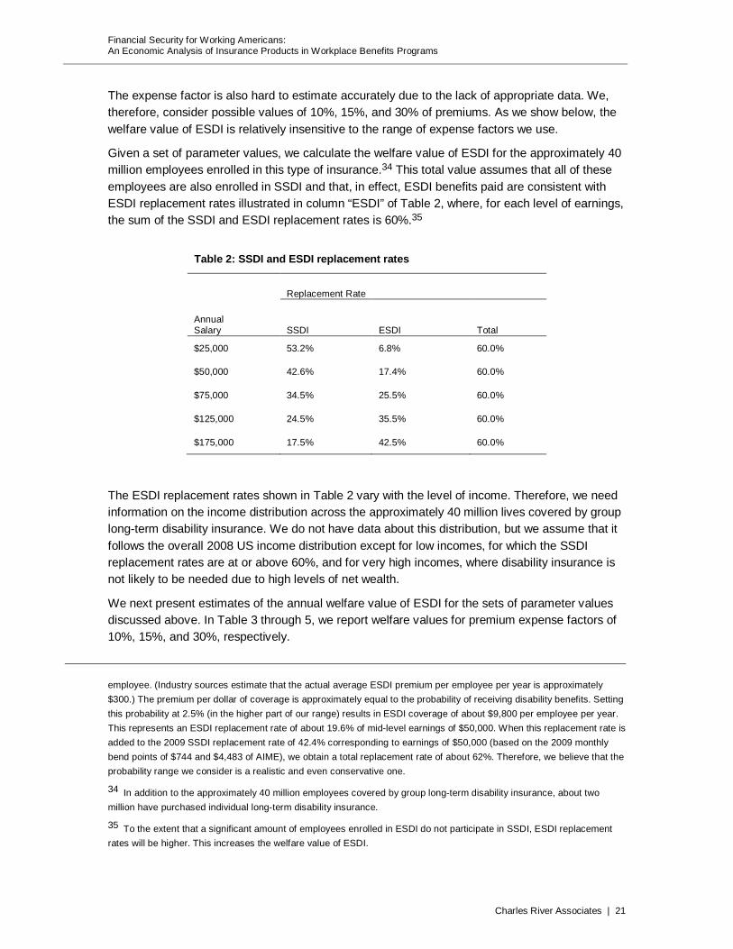
The expense factor is also hard to estimate accurately due to the lack of appropriate data. We, therefore, consider possible values of 10%, 15%, and 30% of premiums. As we show below, the welfare value of ESDI is relatively insensitive to the range of expense factors we use.
Given a set of parameter values, we calculate the welfare value of ESDI for the approximately 40 million employees enrolled in this type of insurance.34 This total value assumes that all of these employees are also enrolled in SSDI and that, in effect, ESDI benefits paid are consistent with ESDI replacement rates illustrated in column “ESDI” of Table 2, where, for each level of earnings, the sum of the SSDI and ESDI replacement rates is 60%.35
Table 2: SSDI and ESDI replacement rates
Replacement Rate
Annual Salary SSDI ESDI Total
$25,000 53.2% 6.8% 60.0%
$50,000 42.6% 17.4% 60.0%
$75,000 34.5% 25.5% 60.0%
$125,000 24.5% 35.5% 60.0%
$175,000 17.5% 42.5% 60.0%
The ESDI replacement rates shown in Table 2 vary with the level of income. Therefore, we need information on the income distribution across the approximately 40 million lives covered by group long-term disability insurance. We do not have data about this distribution, but we assume that it follows the overall 2008 US income distribution except for low incomes, for which the SSDI replacement rates are at or above 60%, and for very high incomes, where disability insurance is not likely to be needed due to high levels of net wealth.
We next present estimates of the annual welfare value of ESDI for the sets of parameter values discussed above. In Table 3 through 5, we report welfare values for premium expense factors of 10%, 15%, and 30%, respectively.
employee. (Industry sources estimate that the actual average ESDI premium per employee per year is approximately $300.) The premium per dollar of coverage is approximately equal to the probability of receiving disability benefits. Setting this probability at 2.5% (in the higher part of our range) results in ESDI coverage of about $9,800 per employee per year. This represents an ESDI replacement rate of about 19.6% of mid-level earnings of $50,000. When this replacement rate is added to the 2009 SSDI replacement rate of 42.4% corresponding to earnings of $50,000 (based on the 2009 monthly bend points of $744 and $4,483 of AIME), we obtain a total replacement rate of about 62%. Therefore, we believe that the probability range we consider is a realistic and even conservative one.
34 In addition to the approximately 40 million employees covered by group long-term disability insurance, about two million have purchased individual long-term disability insurance.
35 To the extent that a significant amount of employees enrolled in ESDI do not participate in SSDI, ESDI replacement rates will be higher. This increases the welfare value of ESDI.

Financial Security for Working Americans: An Economic Analysis of Insurance Products in Workplace Benefits Programs
Charles River Associates | 22
For each table, the prevalence reported in the first column is the prevalence that an employee enrolled in ESDI will receive ESDI payments during a given year. The coefficient of risk aversion used in Table 3 through Table 5 is a measure of the degree of risk aversion in an employee’s utility function. Higher values of this coefficient indicate higher degrees of risk aversion.36 Risk aversion coefficients estimated in empirical work are consistent with the range used in Tables 3 through 9.37
Table 3: Economic welfare value of ESDI (expense factor is 10%)
($ billion per year)
Coefficient of risk aversion Disability prevalence 4.5 5.0 5.5 6.0 6.5 1% $243.9 $310.0 $375.9 $439.2 $498.3
2% $339.2 $408.4 $472.9 $530.9 $581.6
3% $397.7 $464.6 $524.1 $575.3 $617.9
In Table 3, we observe that the welfare value of ESDI in the US is significant, given the size of the industry—40 million employees covered and annual premiums of $9.8 billion for group long-term disability insurance plus an estimated two million lives in individual long-term disability insurance in 2009. At the lower end of the range, this value is approximately $243.9 billion per year; at the higher end of the range, the value is approximately $617.9 billion per year. For a disability prevalence of 2% and risk aversion coefficients between five and six, the value of ESDI is between $408.4 billion and $530.9 billion.
The values in Table 3 are large compared to annual premiums of about $9.8 billion, but it is important to bear in mind that the welfare benefits brought about by the ability to enter into mutually beneficial exchanges can be many times higher than the monetary value exchanged. Insurance is a social institution where mutually beneficial exchanges are arranged so that premiums paid by enrolled individuals are exchanged for coverage payments upon occurrence of the insured event. Insurance companies make this mutually beneficial pooling of resources and exchange possible and charge a factor to cover expenses and normal profits. The exchanges facilitated by the existence of insurance are beneficial because, as measured by expected utility, all insured individuals are better off than they would be without the ability to get insurance. In an efficient insurance industry, the welfare value of insurance will generally be higher than premiums
36 The coefficient of risk aversion in Tables 3 through 5 is referred to as the coefficient of relative risk aversion and measures the rate at which an individual’s marginal utility decreases when wealth is increased by 1%. Marginal utility is defined as the increase in utility per unit of wealth. For risk-averse individuals, additional increases in wealth yield smaller and smaller utility gains. This implies that their marginal utility decreases as wealth increases. Given a 1% increase in wealth, the more risk-averse an individual is (in the relative sense), the higher the percentage decrease in his marginal utility and, therefore, the higher his coefficient of relative risk aversion is.
37 See Sherman D. Hanna and Suzanne Lindamood, “An Improved Measure of Risk Aversion,” Financial Counseling and Planning, Volume 15(2), 2004, pp. 27–38.

Financial Security for Working Americans: An Economic Analysis of Insurance Products in Workplace Benefits Programs
Charles River Associates | 23
paid. As we see in Table 3, the degree of risk aversion is an important determinant of how high this value can be. A high degree of risk aversion means that the welfare losses of adverse outcomes are so high that even a small amount of coverage is very valuable.
The probability of loss is also an important determinant of the welfare value of private insurance. For the prevalence range used in Table 3, the higher this prevalence, the higher the welfare value is.38 In view of the impact that a higher probability of loss has on the welfare value of private insurance, it is important to note that efforts by the insurance industry to reduce the incidence of disability and to get disabled employees back to work faster by means of back-to-work programs aim to effectively reduce the prevalence of loss. While this may reduce the welfare value of private disability insurance, it will also produce an increase in overall social welfare due to a healthier and more productive labor force. We do not analyze the trade-off implied by this comparison in this report, but it is worth mentioning that by improving the efficiency in the marketplace, the insurance industry is likely to extend further the appeal of disability insurance, increasing the number of employees enrolled and the corresponding welfare value. In addition, the best practices developed in the process of implementing back-to-work programs may be successfully applied to the SSDI program, which is struggling with significant backlogs, inefficiencies, and cases of abuse. By reducing the duration of disability, back-to-work programs help lower the disability costs to employers that translates into more competitive value for employees by means of reduced prevalence and expense factors.
These observations about the welfare value of private insurance also apply, with some qualifications because of its very different structure, to SSDI. As in the case of private insurance, SSDI also facilitates the pooling of resources in order to provide disability benefits and, in so doing, it creates welfare value compared to the situation where no social insurance exists. This welfare value could be very large indeed, especially for low income levels, due to the progressive nature of the SSDI benefit formula. And because a lot more employees are enrolled in the SSDI program than in private disability insurance, the overall welfare value of SSDI could possibly be higher than the value of ESDI.
Table 4 reports similar ESDI welfare values for an expense factor of 15%. We observe that values in this case are systematically smaller than the corresponding values in Table 3 but not by much.
38 The reason for this effect is rather technical and related to the fact that the utility schedule exhibits a degree of risk aversion. When the probability of loss is small, as is the case in most insurance markets, the point WE in Figure 1 is close to point W1. As the probability of loss increases, WE decreases and the certainty equivalent without private insurance, WE, decreases by a larger amount. Therefore, the welfare value of insurance, given by (WE − WCE), increases when the probability of loss increases. It is important to note that for unrealistically high values of the probability of loss, the effect discussed runs in the opposite direction, that is, an increase in a high probability of loss results in a smaller welfare value of insurance.
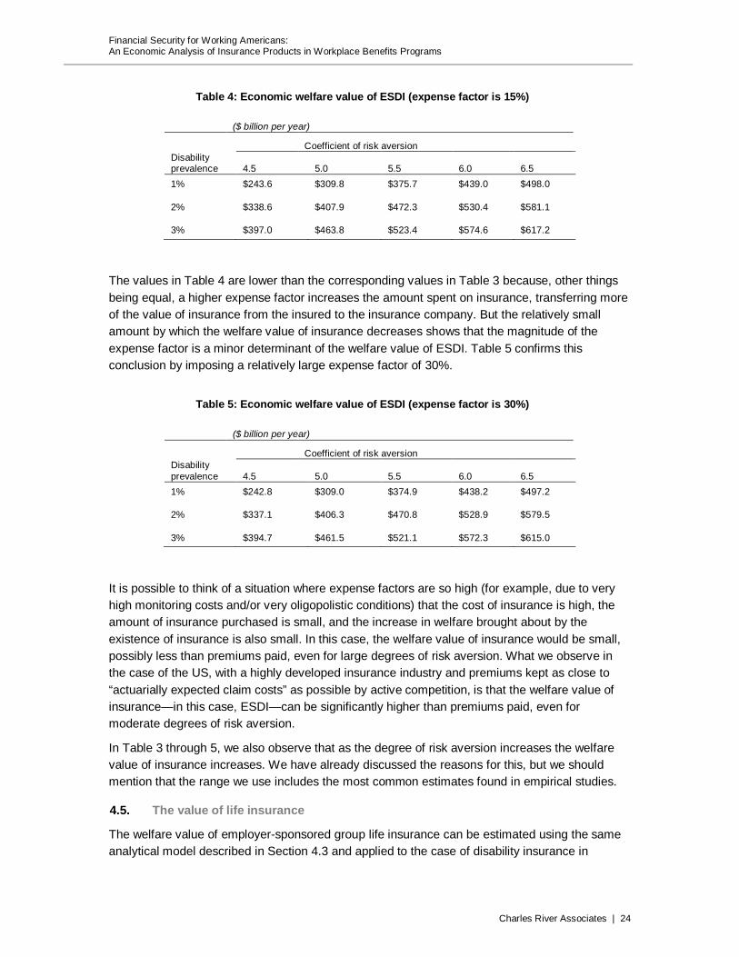
Financial Security for Working Americans: An Economic Analysis of Insurance Products in Workplace Benefits Programs
Charles River Associates | 24
Table 4: Economic welfare value of ESDI (expense factor is 15%)
($ billion per year)
Coefficient of risk aversion Disability prevalence 4.5 5.0 5.5 6.0 6.5 1% $243.6 $309.8 $375.7 $439.0 $498.0
2% $338.6 $407.9 $472.3 $530.4 $581.1
3% $397.0 $463.8 $523.4 $574.6 $617.2
The values in Table 4 are lower than the corresponding values in Table 3 because, other things being equal, a higher expense factor increases the amount spent on insurance, transferring more of the value of insurance from the insured to the insurance company. But the relatively small amount by which the welfare value of insurance decreases shows that the magnitude of the expense factor is a minor determinant of the welfare value of ESDI. Table 5 confirms this conclusion by imposing a relatively large expense factor of 30%.
Table 5: Economic welfare value of ESDI (expense factor is 30%)
($ billion per year)
Coefficient of risk aversion Disability prevalence 4.5 5.0 5.5 6.0 6.5 1% $242.8 $309.0 $374.9 $438.2 $497.2
2% $337.1 $406.3 $470.8 $528.9 $579.5
3% $394.7 $461.5 $521.1 $572.3 $615.0
It is possible to think of a situation where expense factors are so high (for example, due to very high monitoring costs and/or very oligopolistic conditions) that the cost of insurance is high, the amount of insurance purchased is small, and the increase in welfare brought about by the existence of insurance is also small. In this case, the welfare value of insurance would be small, possibly less than premiums paid, even for large degrees of risk aversion. What we observe in the case of the US, with a highly developed insurance industry and premiums kept as close to “actuarially expected claim costs” as possible by active competition, is that the welfare value of insurance—in this case, ESDI—can be significantly higher than premiums paid, even for moderate degrees of risk aversion.
In Table 3 through 5, we also observe that as the degree of risk aversion increases the welfare value of insurance increases. We have already discussed the reasons for this, but we should mention that the range we use includes the most common estimates found in empirical studies.
4.5. The value of life insurance
The welfare value of employer-sponsored group life insurance can be estimated using the same analytical model described in Section 4.3 and applied to the case of disability insurance in
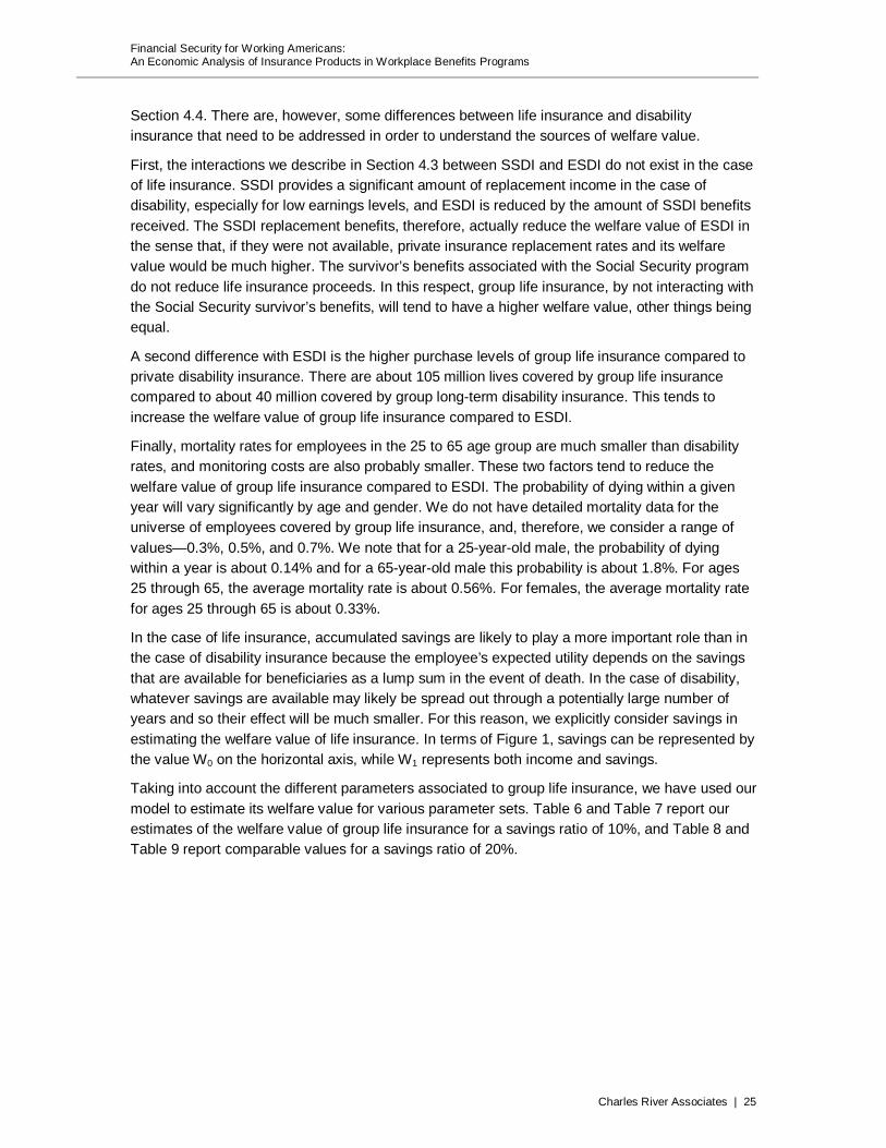
Financial Security for Working Americans: An Economic Analysis of Insurance Products in Workplace Benefits Programs
Charles River Associates | 25
Section 4.4. There are, however, some differences between life insurance and disability insurance that need to be addressed in order to understand the sources of welfare value.
First, the interactions we describe in Section 4.3 between SSDI and ESDI do not exist in the case of life insurance. SSDI provides a significant amount of replacement income in the case of disability, especially for low earnings levels, and ESDI is reduced by the amount of SSDI benefits received. The SSDI replacement benefits, therefore, actually reduce the welfare value of ESDI in the sense that, if they were not available, private insurance replacement rates and its welfare value would be much higher. The survivor’s benefits associated with the Social Security program do not reduce life insurance proceeds. In this respect, group life insurance, by not interacting with the Social Security survivor’s benefits, will tend to have a higher welfare value, other things being equal.
A second difference with ESDI is the higher purchase levels of group life insurance compared to private disability insurance. There are about 105 million lives covered by group life insurance compared to about 40 million covered by group long-term disability insurance. This tends to increase the welfare value of group life insurance compared to ESDI.
Finally, mortality rates for employees in the 25 to 65 age group are much smaller than disability rates, and monitoring costs are also probably smaller. These two factors tend to reduce the welfare value of group life insurance compared to ESDI. The probability of dying within a given year will vary significantly by age and gender. We do not have detailed mortality data for the universe of employees covered by group life insurance, and, therefore, we consider a range of values—0.3%, 0.5%, and 0.7%. We note that for a 25-year-old male, the probability of dying within a year is about 0.14% and for a 65-year-old male this probability is about 1.8%. For ages 25 through 65, the average mortality rate is about 0.56%. For females, the average mortality rate for ages 25 through 65 is about 0.33%.
In the case of life insurance, accumulated savings are likely to play a more important role than in the case of disability insurance because the employee’s expected utility depends on the savings that are available for beneficiaries as a lump sum in the event of death. In the case of disability, whatever savings are available may likely be spread out through a potentially large number of years and so their effect will be much smaller. For this reason, we explicitly consider savings in estimating the welfare value of life insurance. In terms of Figure 1, savings can be represented by the value W0 on the horizontal axis, while W1 represents both income and savings.
Taking into account the different parameters associated to group life insurance, we have used our model to estimate its welfare value for various parameter sets. Table 6 and Table 7 report our estimates of the welfare value of group life insurance for a savings ratio of 10%, and Table 8 and Table 9 report comparable values for a savings ratio of 20%.
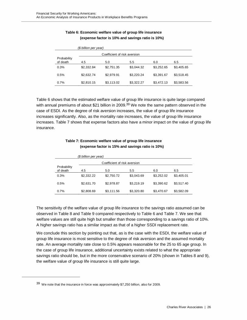
Financial Security for Working Americans: An Economic Analysis of Insurance Products in Workplace Benefits Programs
Charles River Associates | 26
Table 6: Economic welfare value of group life insurance (expense factor is 10% and savings ratio is 10%)
($ billion per year)
Coefficient of risk aversion Probability of death 4.5 5.0 5.5 6.0 6.5 0.3% $2,332.84 $2,751.35 $3,044.32 $3,252.65 $3,405.65
0.5% $2,632.74 $2,979.91 $3,220.24 $3,391.67 $3,518.45
0.7% $2,810.15 $3,113.02 $3,322.27 $3,472.13 $3,583.56
Table 6 shows that the estimated welfare value of group life insurance is quite large compared with annual premiums of about $21 billion in 2009.39 We note the same pattern observed in the case of ESDI. As the degree of risk aversion increases, the value of group life insurance increases significantly. Also, as the mortality rate increases, the value of group life insurance increases. Table 7 shows that expense factors also have a minor impact on the value of group life insurance.
Table 7: Economic welfare value of group life insurance (expense factor is 15% and savings ratio is 10%)
($ billion per year)
Coefficient of risk aversion Probability of death 4.5 5.0 5.5 6.0 6.5 0.3% $2,332.22 $2,750.72 $3,043.69 $3,252.02 $3,405.01
0.5% $2,631.70 $2,978.87 $3,219.19 $3,390.62 $3,517.40
0.7% $2,808.69 $3,111.56 $3,320.80 $3,470.67 $3,582.09
The sensitivity of the welfare value of group life insurance to the savings ratio assumed can be observed in Table 8 and Table 9 compared respectively to Table 6 and Table 7. We see that welfare values are still quite high but smaller than those corresponding to a savings ratio of 10%. A higher savings ratio has a similar impact as that of a higher SSDI replacement rate.
We conclude this section by pointing out that, as is the case with the ESDI, the welfare value of group life insurance is most sensitive to the degree of risk aversion and the assumed mortality rate. An average mortality rate close to 0.5% appears reasonable for the 25 to 65 age group. In the case of group life insurance, additional uncertainty exists related to what the appropriate savings ratio should be, but in the more conservative scenario of 20% (shown in Tables 8 and 9), the welfare value of group life insurance is still quite large.
39 We note that the insurance in force was approximately $7,250 billion, also for 2009.

Financial Security for Working Americans: An Economic Analysis of Insurance Products in Workplace Benefits Programs
Charles River Associates | 27
Table 8: Economic welfare value of group life insurance (expense factor is 10% and savings ratio is 20%)
($ billion per year)
Coefficient of risk aversion Probability of death 4.5 5.0 5.5 6.0 6.5 0.3% $751.96 $1,100.11 $1,458.21 $1,780.71 $2,050.04
0.5% $1,037.80 $1,409.72 $1,753.56 $2,042.82 $2,276.02
0.7% $1,246.52 $1,616.94 $1,940.25 $2,203.55 $2,412.68
Table 9: Economic welfare value of group life insurance (expense factor is 15% and savings ratio is 20%)
($ billion per year)
Coefficient of risk aversion Probability of death 4.5 5.0 5.5 6.0 6.5 0.3% $751.41 $1,099.55 $1,457.65 $1,780.15 $2,049.48
0.5% $1,036.88 $1,408.80 $1,752.64 $2,041.89 $2,275.09
0.7% $1,245.23 $1,615.65 $1,938.95 $2,202.25 $2,411.38
4.6. The value of long-term care insurance
Long-term care (LTC) insurance is designed to pay a share of the costs of care due to chronic illness not covered by traditional health insurance or Medicare. These costs include skilled nursing care, medical equipment, physical and rehabilitation therapy, and the costs of nursing homes or other facilities.
Long-term care costs can be significant. More importantly, they are expected to increase in the near future as the US population ages and baby boomers enter their retirement years. In addition, lack of understanding about the financial impact of long-term care among the public (as well as lack of understanding as to whom pays for it), the relatively large cost of LTC insurance, and the small size of the industry relative to the role played by Medicaid and families themselves are important factors in explaining the currently limited usage of LTC insurance.40
There is ample consensus, however, that individuals should value long-term care insurance quite highly.41 In 2006, about 7% of long-term care expenses were paid by private insurance, with 40%
40 See Howard Gleckman, The Role of Private Insurance in Financing Long-Term Care, Center for Retirement Research at Boston College, September 2007, No. 7-13.
41 Jeffrey R. Brown and Amy Finkelstein, The Private Market for Long-term Care Insurance in the US: A Review of the Evidence, October 2008.

Financial Security for Working Americans: An Economic Analysis of Insurance Products in Workplace Benefits Programs
Charles River Associates | 28
paid by Medicaid and 28% directly paid by families (total expenditures in 2008 were about $230 billion).42 In this report, we have not estimated a value of this type of insurance to the policyholder given the relatively small size of the private insurance market and the uncertainties surrounding its future development.43 These uncertainties include how the government might change its program given the economic strains facing Medicaid, as well as the unanticipated increase in benefit payment costs facing the private insurers due to higher and longer morbidity on the part of policyholders. It is important to note, however, that if the financial impact of long-term care and the sources of financing are properly understood by the public, one should expect the industry to grow, relieving families from the significant, and largely overlooked, burden of out-of-pocket (and the even larger in-kind) expenses.
4.7. The general multi-period model
The single-period model set forth in Section 4.3 carefully and rigorously described how an individual would choose and then value certain types of insurance. While the single-period model provides an excellent exposition of the value of a single set of decisions and outcomes, it cannot inform us regarding decisions and events that happen through a longer period of time. For that examination, we specifically need to employ a multi-period model, which is described in detail in Appendix B.
The multi-period model is highly general. It can take a person of a particular age, income, and savings position and compute the value of ESDI over his or her remaining work life. It does this assuming that the individual has, hypothetically, thousands of lives (more technically, life paths) that are determined by choices and random events. The key random event, of course, is becoming disabled. If this one person could live, say, 1,000 lives, in how many of those 1,000 lives would the person be unlucky and, for example, experience a disabling accident while commuting home from work? Understanding the random nature of disability, the model, consistent with the method outlined in the single-period case, can estimate the certainty-equivalent present value of disability insurance over the remaining span of the employee’s working life. The model can also calculate the probability that the employee would run through his or her existing financial resources and need to access some public assistance program. That probability is a crucial input into estimating the benefit of ESDI to government, a task we address in the next section.
42 Howard Gleckman, Long-Term Care Financing Reform: Lessons from the US and Abroad, The Urban Institute, February 2010, Exhibit 1.
43 Howard Gleckman, Long-Term Care Financing Reform: Lessons from the US and Abroad, The Urban Institute, February 2010.
Financial Security for Working Americans: An Economic Analysis of Insurance Products in Workplace Benefits Programs
Charles River Associates | 29
5. The benefits of employer-supplied disability insurance to government and the taxpayer
5.1. Introduction
The prior section of this study demonstrated the significant economic value to employees of privately supplied disability insurance provided through employers (ESDI). While the value of ESDI to those who actually suffer a disability is readily apparent through the benefit stream that they obtain, even individuals who are fortunate enough never to suffer a work-impeding disability obtain an expected or ex ante value from ESDI through the mere circumstance of being insured against the prospect of such an event. Knowing that you have income protection throughout your working years in the event of a debilitating injury or health condition is worth significantly more to you than the premiums you pay for the coverage, assuming even modest levels of risk aversion. Assuming that the US working population as a whole exhibits, on average, a modest degree of risk aversion, and scaling up the value of private disability insurance to an individual to reflect the overall composition of the US workforce, we find a value for ESDI to the workforce as reported above.
In addition to this enormous value to individuals as employees and consumers, ESDI provides clear benefits to all levels of government (and the taxpayers at large), as it reduces the call on public resources needed to serve the disabled. In addition, it helps maintain the income and assets of some portion of the disabled that then can yield taxes to the government, and it facilitates the functioning of world capital markets.44 This section of the paper reports on some initial efforts to quantify at least a portion of these benefits.
Quantifying the reduction in the call on public resources or the amount of avoided tax losses is an inherently complex endeavor involving an evaluation of the current circumstances and then an estimation of how those would change in the event of a disability with and without ESDI. ESDI’s actual benefit to governments (at all levels) depends on a number of factors, some of which interact with each other. Moreover, the disabled individual can also change his or her response to changes in the situation he or she faces. Finally, while considerable information exists in the public realm, much of the data are estimated or derived from surveys, often for different purposes than what we attempt here. Nevertheless, we believe that the estimates provided here are reasonable and, if anything, understate the benefits to the public monetary resources.
Before proceeding to an examination of the information underlying our estimates, we outline some of the factors and considerations that make quantifying the benefits of ESDI to government and taxpayers challenging.
The first factor to consider is that the benefit a newly disabled person would receive from ESDI depends on decisions the individual will have made before the disabling event, and each employee covered by ESDI makes these choices based on his or her own preferences and circumstances. This includes the fundamental choice of career that implies an expected
44 These considerations are discussed briefly in Sections 5.6 and 5.7.

Financial Security for Working Americans: An Economic Analysis of Insurance Products in Workplace Benefits Programs
Charles River Associates | 30
compensation profile and the prospects of continuing that career in some form with the disability. It would also include choices regarding characteristics of the privately provided disability insurance—the percent of income replaced, whether the premiums are paid with pre- or post-tax dollars (which affects the taxability of the benefits), when the benefit payment stream starts after the disability occurs, and a number of other variables.
A second, even more complicating factor is the overall financial position of the hypothetically newly disabled person’s family at the start of the disability. Some may be fairly young with the potential for decades of work and earnings before them. Others could be middle-aged with substantial obligations arising from children and mortgages. Still others could be in the waning years of their working life with relatively few obligations but high hopes for retirement. Across all of these age cohorts, the non-work-related resources of the newly disabled person will vary substantially. Some, for example, will have very little in the way of available resources to draw on in the event of a period of disability. These have the potential to demand much of the public welfare resources. Others may be quite wealthy and pose no demand on the public resources directly. They could, however, have to reduce their spending and wealth in a way that would reduce income and sales tax receipts for the government. Still others may not have easy access to financial resources but have families or affiliations that can support them in their need.
A third factor involves the nature of choices made after the onset of the disability by the newly disabled person or his or her family. The spouse, for example, might choose to become more—or less—engaged in the working economy. The disabled person can devote greater or lesser efforts to reengaging the workplace—at the previous job or by pursuing new endeavors.
There is, therefore, a wide range of situations and responses to the situations that will ultimately determine the effect of ESDI on public resources.
5.2. Taxpayer-funded benefits in the case of disability
Individuals who become disabled, as indicated previously, are eligible for SSDI. As we have already discussed, the lag between the time of disability that precludes someone from working and the time when that person typically becomes eligible for SSDI is significant. Six months after the onset of disability, only 4.3% of those persons had qualified for SSDI. Twelve months after the onset of disability, only 20.2% had; and two years after the disability, still only 50.3% had qualified for SSDI.45 The provision of ESDI bridges the gap of that time for those covered. In essence, for those that receive SSDI, ESDI provides an interest-free loan while the SSDI application works its way through the system for final determination, and this period of time can be extended.
If ESDI did not exist, some portion of the disabled would need to access public welfare resources to carry them through to the receipt of SSDI, assuming that they ever do become eligible for
45 See GenRe Research, Disability Fact Book, 6th Edition, 2010, p. 65, citing further America’s Health Insurance Plans and the Life and Health Insurance Foundation for Education (prepared by Milliman, Inc.), The Impact of Disability, May 2009, Figure 10, p. 12. Examining all the figures in the cited table, the average time from the onset of disability until the reception of SSDI benefits is at least three years. As the data in the table are truncated at six years of disability duration, and we know that some individuals on long-term disability wait longer than six years to become eligible for SSDI, the actual average will be some unknown but significant amount higher.
Financial Security for Working Americans: An Economic Analysis of Insurance Products in Workplace Benefits Programs
Charles River Associates | 31
SSDI. These would be those who have few other available resources to carry them through the time from the disability to the commencing of SSDI payments.
Government welfare programs provide families and individuals with a certain level of economic resources to attain, or maintain, a (very) modest living. The amounts potentially available, however, are so low as to impose major dislocations of lifestyle and associated costs (both economic and psychological) for those who receive the public assistance. Also, reducing these costs provides the value of ESDI to the individual employee or consumer discussed in Section 4 and the Appendices to this study.
There are a number of different public assistance or welfare programs available, each with its own objectives and eligibility requirements. The welfare benefits provided come from federal, state, and local resources. The major welfare programs available across the country include cash assistance, food assistance, child support, medical assistance, energy or utility assistance, and vocational rehabilitation assistance.
The primary cash assistance program available now is the Temporary Assistance for Needy Families (TANF) program, which was created in 1996 to replace the Aid to Families with Dependent Children (AFDC) and other related welfare programs.46 Another major national welfare assistance program is the Supplemental Nutrition Assistance Program (SNAP), which replaced the so-called Food Stamp program. During fiscal year 2009, “SNAP served approximately 33.5 million people in an average month.”47
Monthly cash assistance under TANF varies with the number of children being supported and by state. For fiscal year 2008, the average monthly cash assistance for all families receiving TANF was $382.95.48
There is considerable overlap between the families that receive TANF, Medicaid, and SNAP. In fiscal year 2008, the latest available information, 97.5% of all families receiving TANF also received public medical assistance, primarily through Medicaid, SCHIP (State Children’s Health Insurance Program), and Medicare. Of all families receiving TANF, 79.1% also received SNAP or Food Stamp benefits. Of the families that received cash assistance through TANF, those also
46 US Department of Health and Human Services, Administration for Children and Families, Office of Family Assistance, Temporary Assistance for Needy Families Program Eighth Annual Report to Congress, June 2009, p. v. Retrieved from http://www.acf.hhs.gov/programs/ofa/data-reports/annualreport8/ar8index.htm in February 2011.
47 US Department of Agriculture, Food and Nutrition Service, Characteristics of Supplemental Nutrition Assistance Program Household: Fiscal Year 2009, Report No. SNAP-10_CHAR, October 2010, pp. xiii and 1. Retrieved from http://www.fns.usda.gov/oane/MENU/Published/SNAP/FILES/Participation/2009Characteristics.pdf in February 2011.
48 US Department of Health and Human Services, Administration for Children and Families, Office of Family Assistance, Characteristics and Financial Circumstances of TANF Recipients, Fiscal Year 2008, Table 41. Retrieved from http://www.acf.hhs.gov/programs/ofa/character/FY2008/tab41.htm in February 2011. For a family with one child, the average monthly cash assistance was $316.70, while for four or more children it was $577.94. Arkansas was the state with the lowest average cash assistance under TANF, while Alaska and Utah had the highest TANF schedules.
Financial Security for Working Americans: An Economic Analysis of Insurance Products in Workplace Benefits Programs
Charles River Associates | 32
receiving SNAP benefits received an average of $292.46 per month in fiscal year 2008.49 “The average monthly SNAP benefit for all participating households in fiscal year 2009 was $276.”50
For purposes of this study, we will assume that any employee suffering a disability that placed him or her in poverty (in a sense to be characterized more concretely below) would need to access both the TANF and SNAP programs if the employee was not covered by ESDI.51 While this varies by family composition (larger families receive more benefits) and state, we will apply the 2008 average monthly amounts presented above ($382.95 for TANF and $292.46 for SNAP) as the minimum government-provided welfare benefit. In other words, without ESDI, each disabled employee that becomes impoverished as a consequence of the disability would draw at least an average of $675 per month from the time that he or she would become eligible for the assistance benefits (within a few months of the disability) until such time as he or she would become eligible for SSDI, assuming that time ever comes. This figure would be $8,100 for each 12-month period and is certainly a low estimate of the public assistance an impoverished disabled person would require.
Many disabled individuals without access to ESDI would need more public assistance than that offered by TANF and SNAP. Almost by definition, a disabled individual will likely be an above-average user of medical services. To the extent that any employer-provided health care continues for the disabled person, that person for that period of time may not need to obtain public medical assistance. To the extent, however, that the disabled individual loses the previously provided medical coverage, or is required to cover some portion of its expense, the disabled individual will likely need to access public medical care. Employers determine the length of time medical care coverage continues in the case of an employee’s disability. Industry sources indicate that medical coverage would be provided typically for a period of up to one year. After employer-provided coverage runs out, the disabled individual would almost certainly need to access public medical care from the Medicaid program or from the Medicare program for those spending two years as SSDI recipients. While the average Medicaid cost per enrollee in 2009 was $6,890, this figure varied by “eligibility group.” The average-aged enrollee incurred $15,678 in spending; the average spent on children was $2,848 and on adults it was $4,123. The “blind/disabled” category of
49 US Department of Health and Human Services, Administration for Children and Families, Office of Family Assistance, Characteristics and Financial Circumstances of TANF Recipients, Fiscal Year 2008, Table 13. Retrieved from http://www.acf.hhs.gov/programs/ofa/character/FY2008/tab13.htm in February 2011. Of the TANF recipients, 14% also obtained housing assistance either in the form of public housing (4.7%) or rent subsidy (9.3%). Of the TANF recipients, 8.0% also received federally subsidized child care benefits. The SNAP benefits varied by state.
50 US Department of Agriculture, Food and Nutrition Service, Characteristics of Supplemental Nutrition Assistance Program Household: Fiscal Year 2009, Report No. SNAP-10_CHAR, October 2010, p. 1. Retrieved from http://www.fns.usda.gov/oane/MENU/Published/SNAP/FILES/Participation/2009Characteristics.pdf in February 2011.
51 A disabled person is also likely to qualify for a number of other public assistance programs. In particular, we know that almost all those receiving TANF are also eligible for Medicaid or Medicare. To understand fully the benefits of ESDI to governments and the taxpayers, we should ideally incorporate figures for all public assistance benefits that a newly disabled individual might access in the absence of ESDI. To date, unfortunately, we have not been able to determine with sufficient accuracy and clarity the likely usage of the other public assistance programs by the newly disabled. For purposes of this study, we very conservatively associate only TANF and SNAP benefits with disability, recognizing that additional public resources are indeed likely consumed by the newly disabled.
Financial Security for Working Americans: An Economic Analysis of Insurance Products in Workplace Benefits Programs
Charles River Associates | 33
Medicaid recipients had the highest overall spending—$16,563 per enrollee.52 While it is clear that disabled individuals are, on average, costly for Medicaid, we cannot determine how the presence of ESDI benefits affects Medicaid usage by the disabled. Clearly the largest effect on Medicaid usage is the continuation of employer-provided health care. But ESDI benefits may raise the disabled family’s income above the level where they would qualify for Medicaid, thus reducing the call on the resources devoted to that program.
Similarly, it is clear that the existence of ESDI reduces the call on the subsidized housing and child care programs by raising the resources of the disabled family above the qualifying level. We lack information, however, on the magnitudes.
Despite the fact that we cannot document the exact figures for medical care, housing, and child care, it is undeniable that ESDI reduces the call on those programs by families affected by disability. Our general knowledge of program costs suggest that the amount per family can be quite large, even exceeding the combined TANF and SNAP payments that we have documented above—at least $675 per month or $8,100 per year. The unknown element is the portion of disabled individuals receiving ESDI whose families would otherwise need to access these other public programs and how intensively they would need to use them. We will investigate the implications of the usage of Medicaid and subsidized housing and child care on a pro forma basis later in this paper.
5.3. Sizing the issue—employment, income, and assets affecting ESDI and public welfare disability insurance
The analysis above provides the rationale for a minimum $675 per month draw on public assistance for a disabled person bereft of income and most savings. Depending on the family size and the circumstances surrounding the use of Medicaid and housing and child care assistance, that monthly draw could be much higher—possibly an average of $1,000 to $1,500 per month. We now need to characterize more fully what constitutes (disability-induced) impoverishment and how many people would suffer such a fate in the absence of ESDI. While addressing all the complexities, subtleties, and interactions in the financial situation of those who benefit from ESDI is difficult, we can gain insight into the financial ramifications by examining available data on the distribution of income, assets, and debt across consumers in the economy. Those employees with lower incomes and fewer savings are at higher risk of impoverishment should they suffer a disability without access to ESDI.
The US Federal Reserve conducted an analysis of consumer finances in 2007 by interviewing 4,422 heads of families. This survey contains the most comprehensive and rigorous information for our needs. The results of this survey are projected to represent the situation of an estimated 116.1 million families in the US at that time.53 Table 10 presents information on the 2007 income,
52 US Department of Health & Human Services, Centers for Medicare & Medicaid Services, Office of the Actuary, 2010 Actuarial Report on the Financial Outlook for Medicaid, December 21, 2010, Table 2, p. 13 (retrieved from http://www.cms.gov/ActuarialStudies/downloads/MedicaidReport2010.pdf in February 2011).
53 Brian K. Bucks, Arthur B. Kennickell, Traci L. Mach, and Kevin B. Moore, “Changes in US Family Finances From 2004 to 2007: Evidence from the Survey of Consumer Finances,” Federal Reserve Bulletin, February 2009, pp. A54–5. The Survey of Consumer Finances has been conducted under the sponsorship of the Federal Reserve every three years since
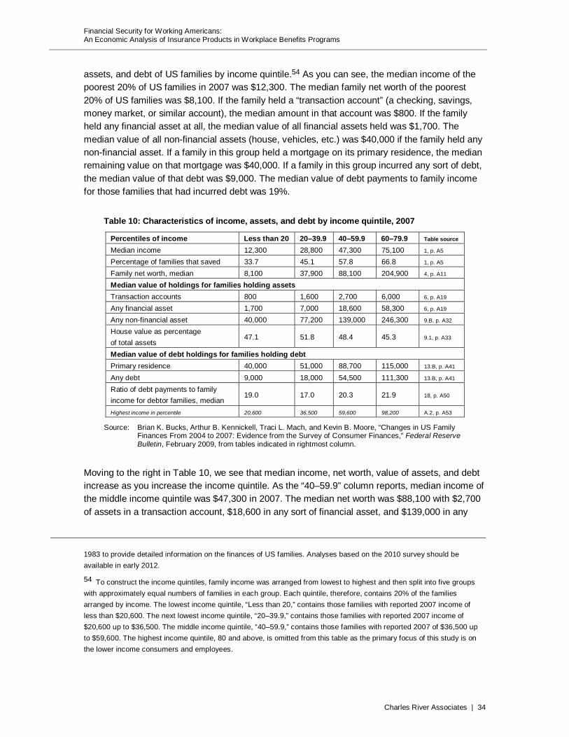
Financial Security for Working Americans: An Economic Analysis of Insurance Products in Workplace Benefits Programs
Charles River Associates | 34
assets, and debt of US families by income quintile.54 As you can see, the median income of the poorest 20% of US families in 2007 was $12,300. The median family net worth of the poorest 20% of US families was $8,100. If the family held a “transaction account” (a checking, savings, money market, or similar account), the median amount in that account was $800. If the family held any financial asset at all, the median value of all financial assets held was $1,700. The median value of all non-financial assets (house, vehicles, etc.) was $40,000 if the family held any non-financial asset. If a family in this group held a mortgage on its primary residence, the median remaining value on that mortgage was $40,000. If a family in this group incurred any sort of debt, the median value of that debt was $9,000. The median value of debt payments to family income for those families that had incurred debt was 19%.
Table 10: Characteristics of income, assets, and debt by income quintile, 2007
Percentiles of income Less than 20 20–39.9 40–59.9 60–79.9 Table source
Median income 12,300 28,800 47,300 75,100 1, p. A5
Percentage of families that saved 33.7 45.1 57.8 66.8 1, p. A5
Family net worth, median 8,100 37,900 88,100 204,900 4, p. A11
Median value of holdings for families holding assets Transaction accounts 800 1,600 2,700 6,000 6, p. A19
Any financial asset 1,700 7,000 18,600 58,300 6, p. A19
Any non-financial asset 40,000 77,200 139,000 246,300 9.B, p. A32
House value as percentage of total assets
47.1 51.8 48.4 45.3 9.1, p. A33
Median value of debt holdings for families holding debt Primary residence 40,000 51,000 88,700 115,000 13.B, p. A41
Any debt 9,000 18,000 54,500 111,300 13.B, p. A41
Ratio of debt payments to family income for debtor families, median
19.0 17.0 20.3 21.9 18, p. A50
Highest income in percentile 20,600 36,500 59,600 98,200 A.2, p. A53
Source: Brian K. Bucks, Arthur B. Kennickell, Traci L. Mach, and Kevin B. Moore, “Changes in US Family Finances From 2004 to 2007: Evidence from the Survey of Consumer Finances,” Federal Reserve Bulletin, February 2009, from tables indicated in rightmost column.
Moving to the right in Table 10, we see that median income, net worth, value of assets, and debt increase as you increase the income quintile. As the “40–59.9” column reports, median income of the middle income quintile was $47,300 in 2007. The median net worth was $88,100 with $2,700 of assets in a transaction account, $18,600 in any sort of financial asset, and $139,000 in any
1983 to provide detailed information on the finances of US families. Analyses based on the 2010 survey should be available in early 2012.
54 To construct the income quintiles, family income was arranged from lowest to highest and then split into five groups with approximately equal numbers of families in each group. Each quintile, therefore, contains 20% of the families arranged by income. The lowest income quintile, “Less than 20,” contains those families with reported 2007 income of less than $20,600. The next lowest income quintile, “20–39.9,” contains those families with reported 2007 income of $20,600 up to $36,500. The middle income quintile, “40–59.9,” contains those families with reported 2007 of $36,500 up to $59,600. The highest income quintile, 80 and above, is omitted from this table as the primary focus of this study is on the lower income consumers and employees.

Financial Security for Working Americans: An Economic Analysis of Insurance Products in Workplace Benefits Programs
Charles River Associates | 35
non-financial asset (including the primary residence). As you look across the income quintiles, the house value as a percent of total assets and the ratio of debt payments to family income are notably stable.
Table 11 presents the information gathered in the survey grouped by net worth quartile.55 In other words, instead of grouping the families by income and observing their resulting assets and net worth, this table groups the families by net worth in order to observe the change in income, assets, and debt. This confirms the stylized fact of economics that as net worth increases, so does median income, asset value, and debt. This is not to say that the causality runs directly from net worth to income; the more direct linkage works from income to net worth, but that higher income is associated with higher net worth and vice versa.
Table 11: Characteristics of income, assets, and debt by net worth quartile, 2007
Percentiles of net worth: Less than 25 25–49.9 50–74.9 75–89.9 Table source
Median income 23,600 41,000 56,700 82,300 1, p. A5
Percentage of before-tax family income from wages
79.9 79.9 77.8 72.4 2. p. A7
Percentage of families that saved 40.4 52.9 59.0 69.0 1, p. A5
Family net worth, median 1,200 54,200 219,800 571,400 4, p. A11
Median value of holdings for families holding assets Transaction accounts 700 2,000 6,100 15,500 6, p. A19
Any financial asset 1,400 13,200 59,600 215,000 6, p. A19
Any non-financial asset 8,600 95,800 229,100 443,700 9.B, p. A32
Median value of debt holdings for families holding debt Primary residence 107,000 85,000 104,00 130,000 13.B, p. A41
Any debt 11,900 64,200 97,500 127,000 13.B, p. A41
Ratio of debt payments to family income for debtor families, median
12.1 23.4 21.5 18.2 18, p. A50
Highest net worth in percentile 14,100 120,300 372,000 908,200 A.2, p. A53
Source: Brian K. Bucks, Arthur B. Kennickell, Traci L. Mach, and Kevin B. Moore, “Changes in U.S. Family Finances From 2004 to 2007: Evidence from the Survey of Consumer Finances,” Federal Reserve Bulletin, February 2009, from tables indicated in rightmost column.
Finally, Table 12 looks at the same information but groups it according to age cohort. As age increases, so does income, family net worth, and asset value. This is the organization of the survey data we will use for this study, as it is chronological and comports with the needs of the multi-period model. Ideally, we would want to examine age cohorts by income distribution. While income and assets generally increase with age, in each age cohort there are some families whose income and net worth remain quite low while others advance financially. Those families with the lowest income and net worth in each age cohort are most likely to face financial stress, and possibly ruin, in the situation where a major income producer suffers a work-impeding
55 Where quintile divides the total assemblage into five approximately equally sized groups, quartile divides the total into four approximately equally sized groups. The survey actually splits the highest net worth quartile into two parts—75th through 89.9 percentiles and 90th and above. The highest grouping, 90th percentile and above, is omitted from this table.
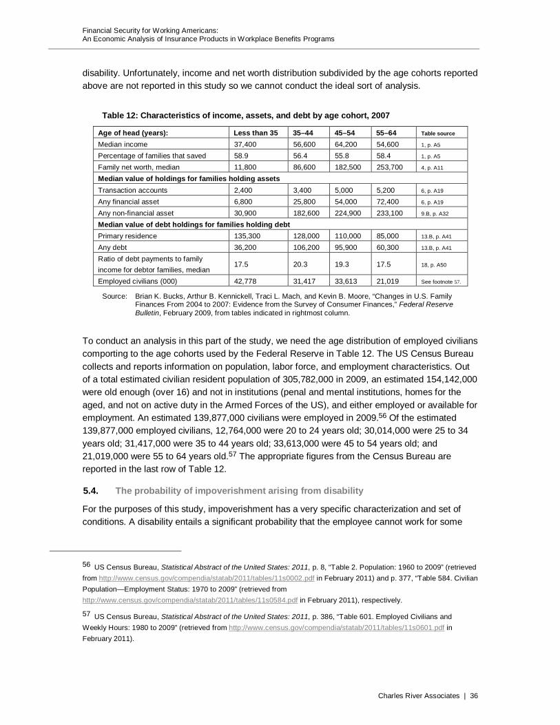
Financial Security for Working Americans: An Economic Analysis of Insurance Products in Workplace Benefits Programs
Charles River Associates | 36
disability. Unfortunately, income and net worth distribution subdivided by the age cohorts reported above are not reported in this study so we cannot conduct the ideal sort of analysis.
Table 12: Characteristics of income, assets, and debt by age cohort, 2007
Age of head (years): Less than 35 35–44 45–54 55–64 Table source
Median income 37,400 56,600 64,200 54,600 1, p. A5
Percentage of families that saved 58.9 56.4 55.8 58.4 1, p. A5
Family net worth, median 11,800 86,600 182,500 253,700 4, p. A11
Median value of holdings for families holding assets Transaction accounts 2,400 3,400 5,000 5,200 6, p. A19
Any financial asset 6,800 25,800 54,000 72,400 6, p. A19
Any non-financial asset 30,900 182,600 224,900 233,100 9.B, p. A32
Median value of debt holdings for families holding debt Primary residence 135,300 128,000 110,000 85,000 13.B, p. A41
Any debt 36,200 106,200 95,900 60,300 13.B, p. A41
Ratio of debt payments to family income for debtor families, median
17.5 20.3 19.3 17.5 18, p. A50
Employed civilians (000) 42,778 31,417 33,613 21,019 See footnote 57.
Source: Brian K. Bucks, Arthur B. Kennickell, Traci L. Mach, and Kevin B. Moore, “Changes in U.S. Family Finances From 2004 to 2007: Evidence from the Survey of Consumer Finances,” Federal Reserve Bulletin, February 2009, from tables indicated in rightmost column.
To conduct an analysis in this part of the study, we need the age distribution of employed civilians comporting to the age cohorts used by the Federal Reserve in Table 12. The US Census Bureau collects and reports information on population, labor force, and employment characteristics. Out of a total estimated civilian resident population of 305,782,000 in 2009, an estimated 154,142,000 were old enough (over 16) and not in institutions (penal and mental institutions, homes for the aged, and not on active duty in the Armed Forces of the US), and either employed or available for employment. An estimated 139,877,000 civilians were employed in 2009.56 Of the estimated 139,877,000 employed civilians, 12,764,000 were 20 to 24 years old; 30,014,000 were 25 to 34 years old; 31,417,000 were 35 to 44 years old; 33,613,000 were 45 to 54 years old; and 21,019,000 were 55 to 64 years old.57 The appropriate figures from the Census Bureau are reported in the last row of Table 12.
5.4. The probability of impoverishment arising from disability
For the purposes of this study, impoverishment has a very specific characterization and set of conditions. A disability entails a significant probability that the employee cannot work for some
56 US Census Bureau, Statistical Abstract of the United States: 2011, p. 8, “Table 2. Population: 1960 to 2009” (retrieved from http://www.census.gov/compendia/statab/2011/tables/11s0002.pdf in February 2011) and p. 377, “Table 584. Civilian Population—Employment Status: 1970 to 2009” (retrieved from http://www.census.gov/compendia/statab/2011/tables/11s0584.pdf in February 2011), respectively.
57 US Census Bureau, Statistical Abstract of the United States: 2011, p. 386, “Table 601. Employed Civilians and Weekly Hours: 1980 to 2009” (retrieved from http://www.census.gov/compendia/statab/2011/tables/11s0601.pdf in February 2011).

Financial Security for Working Americans: An Economic Analysis of Insurance Products in Workplace Benefits Programs
Charles River Associates | 37
period of time and therefore will not earn income. The employee may have accumulated vacation or sick leave time from the job, but this will under most circumstances run out. For our purposes, any accumulated vacation or sick time is part of the employee’s wage compensation. Lacking income, the employee’s family will be forced to rely on any accumulated savings available. As reported in Table 10 through Table 12, however, tens of millions of employees and their families have very limited savings to fall back on. Survey and anecdotal information confirm the limited financial cushion many families have in the event of a loss of income.
“More than a quarter (27%) of working Americans say they would have trouble supporting themselves financially ‘immediately’ following a disability that keeps them out of work while nearly half (49%) would reach that point in a month or less. Three out of four (74%) would face financial trouble within six months.”58
“Seven in 10 workers could not cover their normal living expenses for more than six months” in the event they lost their source of income.59
“Ninety-five percent of those surveyed would need to make some lifestyle changes if they lost part of their families’ income, and two-thirds of those changes would need to be significant.”60
“Eight in 10 workers are concerned about how they would pay their living expenses if they had to miss work for six months or longer due to disability.”61
Approximately one-half of Americans surveyed in 2009 reported that they were either certainly or probably not able to come up with $2,000 in cash within thirty days. Nearly one-quarter of the households making between $100,000 and $150,000 claimed an inability to raise $2,000 cash in a month.62
Using the multi-period model described in Section 4.7 and Appendix B, we characterize impoverishment arising from disability as the point in time when the disabled family has insufficient income or assets available to pay the bills associated with a modest living (defined as $14,710 per year). At this point, absent ESDI benefits or help from family or charitable organizations, the family would have to rely on some level of public welfare assistance to pay
58 GenRe Research, Disability Fact Book, 6th Edition, 2010, p. 19, citing further LIFE Foundation Press Release, Hit Hard by the Economy, Americans Risk Knockout Without Disability Insurance, May 2009 (based on an online survey poll of 1,007 Americans ages 18 and over).
59 GenRe Research, Disability Fact Book, 6th Edition, 2010, p. 20, citing further Council for Disability Awareness, Worker Disability Planning and Preparedness Study, 2008 (based on an online survey of 1,448 full-time working US adults ages 21 to 65).
60 GenRe Research, Disability Fact Book, 6th Edition, 2010, p. 20, citing further The Hartford, The Hartford’s Benefit Landscape Study: Economy and Stress, March 2010 (based on an online survey of 1,000 adults).
61 GenRe Research, Disability Fact Book, 6th Edition, 2010, p. 20, citing further Council for Disability Awareness, Worker Disability Planning and Preparedness Study, 2008 (based on an online survey of 1,448 full-time working US adults ages 21 to 65).
62 Annamarie Lusardi, Daniel J. Schneider and Peter Tufano, “Financially Fragile Households: Evidence and Implications,” National Bureau of Economic Research Working Paper 17072, May 2011.
Financial Security for Working Americans: An Economic Analysis of Insurance Products in Workplace Benefits Programs
Charles River Associates | 38
current shelter, food, and clothing costs. Those with lower incomes and fewer assets are more likely to face impoverishment in a disability situation. Younger people, on average, have lower incomes and fewer assets than older people, although they are also less likely to become disabled. Public assistance programs are actually designed to make families eligible for assistance before the point they exhaust all assets. Excluding this earlier likely access to public assistance is another instance of reducing the call on public assistance resources embedded in this analysis. Ideally we would incorporate this element, but the information needed to make reasonable calculations is not available. With this understanding, we acknowledge another instance of conservatism in the analysis—we are using figures for the call on public assistance resources that are in all likely lower than the actual resources needed.
5.5. First estimates of the short-term benefits of ESDI—easing the burden on public assistance programs
Our initial estimates of the short-term benefits of ESDI outline the avoided burden on public assistance programs arising because families have access to privately supplied disability insurance benefits. These estimates are based on the figures and analysis presented above combined with the information presented below.
Not all employees have access to disability insurance through their employers. The US Bureau of Labor Statistics estimated in 2010 that 37% of civilian workers had access to short-term disability while 33% had access to long-term disability insurance. Of those employees that had access to these types of insurance, nearly all (97%) participated—36% of all civilian employees participated in short-term disability insurance while 32% of all civilian employees participated in long-term disability insurance.63
Estimates of the incidence and severity of disability vary. One source estimates that the chances that any person will experience at least one episode of a long-term disability (one of at least 90 days) before the age of 65 ranges between one in three (for older workers) and one in two (for younger workers with a longer expected work life).64 In any one year, however, the incidence of an initial disabling event (accident or illness) is considerably less, but it does increase with age. For example, for employees under the age of 35, there are less than four long-term disability claims per thousand. This figure rises with age so that employees over the age of 55 experience 10 or more long-term disability claims per thousand.65 Short-term disability claims, however, are far more frequent. In 2009, for example, while there was an average of 5.3 long-term disability claims per 1,000 insured lives, there was also an average of 58.4 short-term disability claims per 1,000 insured lives.66
63 US Bureau of Labor Statistics, Employee Benefits Survey: Life, Short-Term Disability, and Long-Term Disability Insurance Benefits, March 2010, Table 17 (retrieved from http://www.bls.gov/ncs/ebs/benefits/2010/ownership/civilian/table12a.pdf in February 2011).
64 GenRe Research, Disability Fact Book, 6th Edition, 2010, p. 18, citing further Donald F. Cady, 2010 Field Guide to Estate, Employee & Business Planning, National Underwriter Company, 2010.
65 GenRe Research, Disability Fact Book, 6th Edition, 2010, p. 36, citing further GenRe, Analysis of 1987 GLTD Table.
66 GenRe Research, Disability Fact Book, 6th Edition, 2010, p. 36, citing further GenRe, US Group Disability Rate & Risk Management Survey. It is important to note that these figures are new claims incidence rates and not the cumulative
Financial Security for Working Americans: An Economic Analysis of Insurance Products in Workplace Benefits Programs
Charles River Associates | 39
To estimate the short-term benefits of ESDI, we first determine the number of new disability incidents over the course of a period of, say, a year. We know from the US Census Bureau that there were approximately 128.9 million civilian employees between the ages of 20 and 64 in 2009. We also know that 32% of these had long-term disability insurance, so approximately 40 million civilian employees were covered.67 Moreover, these employees had a long-term disability incidence of in the range of three to six per thousand insured (around .05%). This means that between 120,000 and 240,000 civilian employees suffered from a new disabling event at some point in 2009 that would end up being a long-term situation (generally over 90 or 180 days).68
Not every employee suffering a new disabling incident in 2009 would suffer impoverishment. Those suffering a long-term disability, holding all else equal, have a higher probability of slipping into poverty. The multi-period model described in Appendix B suggests that at least 70%, and possibly up to 90%, of individuals facing long-term disability would face impoverished circumstances requiring access to public assistance programs in the absence of ESDI.69 Using the midpoint of this range, 80%, as the portion of disabled individuals covered by ESDI who would otherwise need to use extensive public assistance, somewhere between 96,000 and 192,000 families are affected.70 As this is long-term disability, on average the disabled individuals will need assistance for more than the first year, and a new set of disabled individuals will need to be included in the calculations. Conservatively assuming that there are always at least three years of disabled individuals receiving ESDI that would otherwise be on public assistance, the number of families that avoid using public assistance programs as a consequence of ESDI ranges between 280,000 and 575,000 in each year.71 At an average amount of $8,100 per year,
prevalence rates that include claims paid in a given year for disability from prior years. A group of leading long-term disability insurance companies reported that they were providing 627,000 disabled individuals with insurance payments in 2009. (Council for Disability Awareness, 2010 Long-Term Disability Claims Review, p. 1.)
67 Industry sources indicate that approximately two million people purchase long-term disability insurance on an individual basis.
68 “141,000 new disabled individuals were approved by reporting CDA Member Companies for long-term disability insurance claim benefits in 2009.” Of these disability claims, 95% were not work-related and 31.2% of the individuals on long-term disability insurance did not qualify for SSDI payments. Council for Disability Awareness, 2010 Long-Term Disability Claims Review, p. 2.
We also know that 36% of the 128.9 million civilian employees in 2009 (or 46.4 million) had short-term disability insurance. These 46.4 million had an incidence of short-term disability of 58.4 per thousand insured (not quite 6%). This means that 2.7 million insured employees suffered a new short-term disability of some sort.
69 These results will be narrowed and quantified more precisely as the model undergoes additional vetting and refinement.
70 Using the 141,000 figure for new disability claims in 2009 cited in footnote 68, the analogous number is approximately 113,000 families.
71 Analysis supporting the three year figure is presented in footnote 45. Using the 141,000 figure for new disability claims in 2009 cited in footnote 68, the analogous number is approximately 330,000 families.

Financial Security for Working Americans: An Economic Analysis of Insurance Products in Workplace Benefits Programs
Charles River Associates | 40
the reduction in public assistance for the long-term disabled as a consequence of their having ESDI ranges between $2.25 and $4.5 billion per year.72
On a very conservative basis, ESDI relieves US public assistance of at least $3 billion per year in expenditures.73 As suggested above, the average public assistance benefit of $675 per month (or $8,100 per year) is very likely a low estimate of the total public assistance benefits that ESDI replaces. If, for example, the actual average public assistance benefits replaced by ESDI is $12,000 per year (not quite 50% higher than the figure we used), we can arrive at an estimate of between $3.3 and $6.8 billion per year of ESDI relief for public assistance.
This estimate of public assistance benefits arises with a participation rate for ESDI of one-third or less. To the extent that a larger portion of US civilian employees participate in ESDI insurance programs, the reduction in the demand for public assistance would increase.
5.6. Possible, but not-yet-quantifiable, long-term benefits of ESDI—preserving income and wealth of the newly disabled yielding more tax revenue
In addition to relieving the burden on public assistance resources, ESDI helps maintain the income and assets of some portion of the disabled that then can yield direct or indirect taxes to the government. First, under some circumstances, ESDI benefits are taxable income and contribute directly to the tax receipts of government. ESDI benefits are taxable if the premiums for ESDI coverage are deducted from either the employer’s or employee’s income before taxes. Comprehensive data on the amount of ESDI subject to income taxes are not available. Nevertheless, some portion of the over $8 billion per year in long-term disability payments is subject to direct taxation at both the federal and state levels.
Even in the situation where ESDI benefit payments are not included in taxable income because the premiums were paid on an after-tax basis, the ESDI benefit payments can result in additional tax receipts by the government. As described previously, SSDI payments are capped at a modest level. Someone whose career-earning prospects were bright will find that SSDI payments are low enough that they will lower their consumption of goods and services or draw down any assets accumulated pre-disability or both.
The extra income that ESDI provides the disabled individuals replaces more of the work income lost than SSDI. As a natural consequence of this additional income, the disabled can buy more, leading to sales tax receipts for state and local governments. In other words, non-taxable ESDI benefit payments above and beyond the SSDI benefits facilitate purchases of goods and services, some portion of which will generate sales and excise taxes to government coffers. Here again, there are insufficient data available to quantify these government receipts.
72 Using the 141,000 figure for new disability claims in 2009 cited in footnote 68 above, the analogous figure is $2.7 billion per year.
73 By way of comparison, insurers representing roughly 75% of the commercial disability insurance business paid $8.1 billion in long-term insurance claim payments to disabled individuals in 2009. Council for Disability Awareness, 2010 Long-Term Disability Claims Review, p. 1. In 2009, long-term disability premiums were $9.8 billion while short-term disability premiums were $3.8 billion. Given typical expense factors, this magnitude of benefit to the government and taxpayer of ESDI seems quite reasonable. GenRe Research, Disability Fact Book, 6th Edition, 2010, p. 4, citing further GenRe, 2009 US Group Disability Market Survey.

Financial Security for Working Americans: An Economic Analysis of Insurance Products in Workplace Benefits Programs
Charles River Associates | 41
Finally, the additional income from ESDI will also allow the disabled to maintain higher savings balances to the extent that the individual had them before the disability. Savings balances, in turn, lead to interest, dividend, and capital gain income on the part of individuals. To the extent that non-taxable ESDI benefit payments maintain savings balances, taxable income from the savings will be higher. This, in turn, leads to higher income tax revenues at both the federal and state level, all else being held equal.
While all of these tax receipt benefits, in principle, arise from the provision of ESDI, data to determine their magnitudes are not yet available.
Society as a whole obtains additional benefits from ESDI that are above and beyond those quantifiable (in principle) from tax receipts or reduced public assistance. ESDI allows families to maintain something closer to their “normal” standard of living than they would without this sort of income protection. That means that bills get paid, foreclosures are avoided, and dislocations (both physical and psychological) are minimized. The hardships of suffering through a disability are challenging enough. While ESDI or other forms of disability insurance cannot erase the consequences, they can ease the burden—particularly the financial burden—considerably.
5.7. The capital market benefits of employer-sponsored insurance
Our discussion so far has focused on the value of employer-sponsored insurance products and their ability to create public sector savings. Separate from these benefits, and in addition to them, there are significant benefits for society as a whole that derive from the prominent role that the private insurance industry plays in the capital markets. The US and the UK insurance industries are respectively the largest and third largest in the world, accounting for 28% and 8% respectively of worldwide premium income in 2009. (Japan has the second largest insurance industry, accounting for 13% of 2009 worldwide premium income). The very large reserves held by insurance companies are invested in the US, the UK, and the international capital markets, contributing to their depth and liquidity and facilitating the growth of businesses.
The insurance industry, as a whole, occupies a leading position in the world capital markets. They own a large chunk of all corporate bonds and privately placed fixed income securities. Their annual fixed income investment needs supplies much of the demand for government, corporate and mortgage-related debt as well as a notable amount of equities.74 The workplace benefit programs examined in this study are a significant component of the insurance industry and therefore are a participant in the world capital markets.
74 See, for example, Anthony M. Santomero and David F. Babbel, Financial Markets, Instruments, and Institutions, 2nd Edition, McGraw-Hill Irwin, pp. 563–4.
Financial Security for Working Americans: An Economic Analysis of Insurance Products in Workplace Benefits Programs
Charles River Associates | 42
6. Conclusion
Attaining, and then maintaining, the American Dream is neither assured nor easy. To pursue financial freedom and security in today’s society, individuals must enhance their human capital through education and training. They must then find an occupation that will convert their human capital into income so they can purchase food, shelter, and the various comforts in life. Along the way, many will form families and enter into long-term financial commitments such as holding a mortgage, making car payments, etc. If fortunate, at the end of their working lives, they can retire and spend at least some portion of their last days in comfort.
Unfortunately, obstacles can arise and hinder the attainment of the American Dream for many. As recent experience has demonstrated, the economy can fail or nature can wreak havoc—destroying lives, property, jobs, and plans. Catastrophes need not affect entire economies or substantial geographic areas to pose significant problems for individuals, however. An accident such as a car wreck, a fire, or a fall can both destroy an asset and cause injury to a person. A debilitating illness can place a person under medical care and stop him or her from earning income. For most individuals and families, such personal catastrophes can rapidly deplete existing assets and preclude them from making a living. And the fact is that a very small portion of the population has accumulated assets sufficient to cover the lost income from their own resources. Individuals at the beginning of their careers have not had enough time to acquire savings, and many in the middle of their careers have committed their savings (and future income) to supporting families, car payments, college tuition repayments, mortgages, etc.
Various forms of insurance have evolved over the centuries to provide protection against the misfortunes that may befall us. As individuals, we can purchase a wide variety of insurance products to replace property (e.g., homes and automobiles), pay others for services (e.g., medical care), or provide income under specific circumstances (e.g., life insurance and annuities). As a society we have also charged governments with providing various types of social insurance (e.g., public assistance, medical care for the aged and indigent, retirement income, etc.). A third, and often overlooked, channel of insurance protection is that facilitated by employers. This study provides a needed economic analysis into the benefits of employer-sponsored insurance programs for employees (and their families), the government, and the employers themselves.
Using standard tools of economic analysis applied to insurance, this study demonstrated a likely welfare value of employer-sponsored group disability insurance ranging from a minimum of $230 billion up to about $590 billion per year for the approximately 40 million employees covered. Likewise, employer-sponsored group life insurance provides economic value of $1.25 trillion to $3.5 trillion annually to the approximately 105 million people covered. Other employer-facilitated insurance (accidental death and dismemberment, cancer and critical illness, and long-term care, for example) also provide substantial value to those covered, although their usage is relatively limited.
Employer-sponsored disability insurance also provides significant benefits to society at large as benefit payments from this program substantially reduces the call on public assistance resources. Annual group long-term disability premiums of approximately $10 billion per year help hundreds of thousands of families avoid calling on public assistance and thereby reduces the burden on
Financial Security for Working Americans: An Economic Analysis of Insurance Products in Workplace Benefits Programs
Charles River Associates | 43
these programs by $2.25 to $4.5 billion per year. In addition, of course, the actual recipients of group long-term disability insurance benefits can maintain a much higher standard of living than if they had to rely solely on government disability and public assistance programs. Finally, employers gain from a workforce that is better protected from adverse events, be they work-related or not. Employers can offer access to insurance at attractive rates and substantial convenience, which is an advantage when competing in the labor market for talent.
The provision or facilitation of various insurance products in workplace benefit programs in the US supplies substantial returns to all involved in the process.
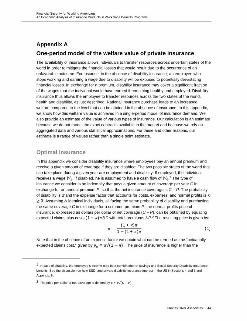
Financial Security for Working Americans: An Economic Analysis of Insurance Products in Workplace Benefits Programs
Charles River Associates | 44
Appendix A One-period model of the welfare value of private insurance The availability of insurance allows individuals to transfer resources across uncertain states of the world in order to mitigate the financial losses that would result due to the occurrence of an unfavorable outcome. For instance, in the absence of disability insurance, an employee who stops working and earning a wage due to disability will be exposed to potentially devastating financial losses. In exchange for a premium, disability insurance may cover a significant fraction of the wages that the individual would have earned if remaining healthy and employed. Disability insurance thus allows the employee to transfer resources across the two states of the world, health and disability, as just described. Rational insurance purchase leads to an increased welfare compared to the level that can be attained in the absence of insurance. In this appendix, we show how this welfare value is achieved in a single-period model of insurance demand. We also provide an estimate of the value of various types of insurance. Our calculation is an estimate because we do not model the exact contracts available in the market and because we rely on aggregated data and various statistical approximations. For these and other reasons, our estimate is a range of values rather than a single point estimate.
Optimal insurance In this appendix we consider disability insurance where employees pay an annual premium and receive a given amount of coverage if they are disabled. The two possible states of the world that can take place during a given year are employment and disability. If employed, the individual receives a wage 푊 . If disabled, he is assumed to have a cash flow of 푊 .1 The type of insurance we consider is an indemnity that pays a given amount of coverage per year C in exchange for an annual premium P, so that the net insurance coverage is C – P. The probability of disability is π and the expense factor that accounts for costs, expenses, and normal profits is κ ≥ 0. Assuming N identical individuals, all facing the same probability of disability and purchasing the same coverage C in exchange for a common premium P, the normal-profits price of insurance, expressed as dollars per dollar of net coverage (C – P), can be obtained by equating expected claims plus costs (1 + 휅)휋푁퐶 with total premiums NP.2 The resulting price is given by:
푝 = (1 + 휅)휋
1 − (1 + 휅)휋 (1)
Note that in the absence of an expense factor we obtain what can be termed as the “actuarially expected claims cost,” given by 푝 = 휋 (1 − 휋)⁄ . The price of insurance is higher than the
1 In case of disability, the employee’s income may be a combination of savings and Social Security Disability Insurance benefits. See the discussion on how SSDI and private disability insurance interact in the US in Sections 4 and 5 and Appendix B.
2 The price per dollar of net coverage is defined by 푝 = 푃 (퐶 − 푃)⁄ .
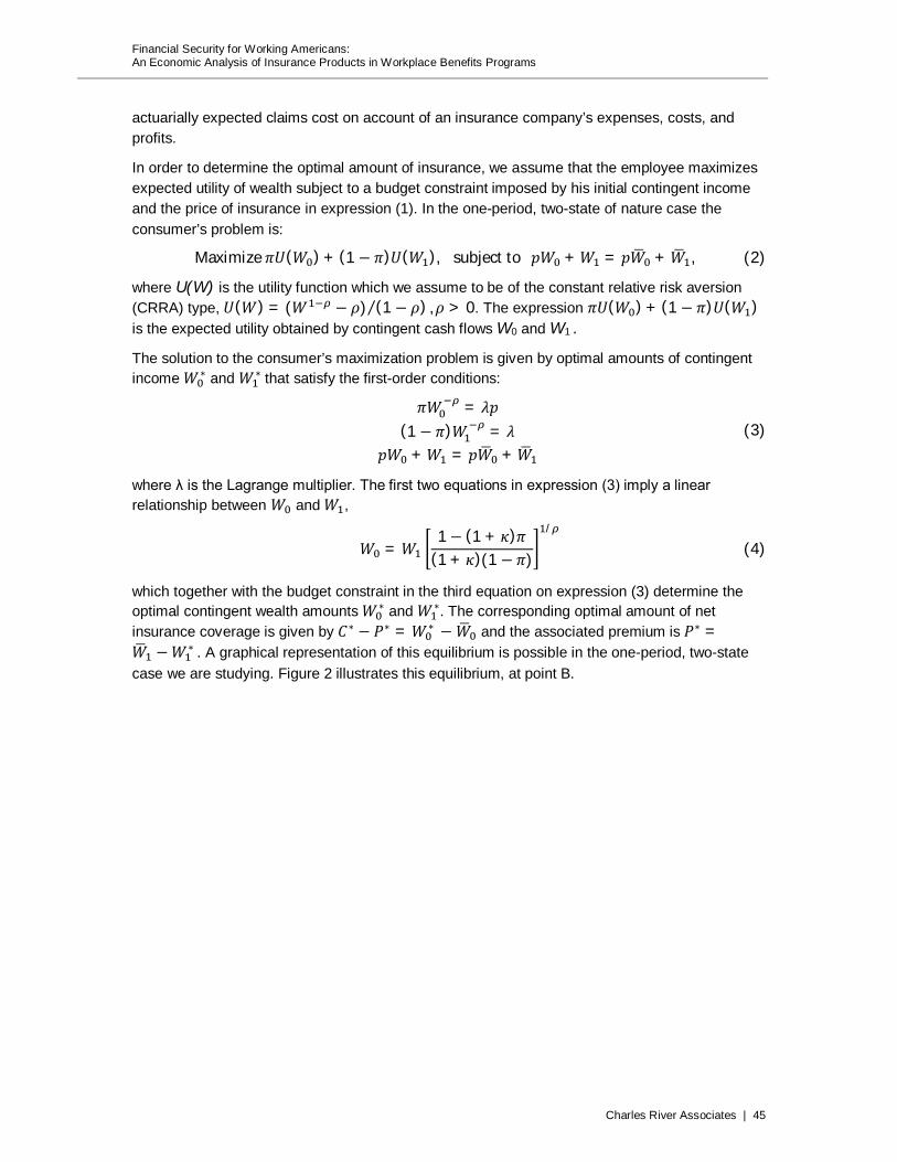
Financial Security for Working Americans: An Economic Analysis of Insurance Products in Workplace Benefits Programs
Charles River Associates | 45
actuarially expected claims cost on account of an insurance company’s expenses, costs, and profits.
In order to determine the optimal amount of insurance, we assume that the employee maximizes expected utility of wealth subject to a budget constraint imposed by his initial contingent income and the price of insurance in expression (1). In the one-period, two-state of nature case the consumer’s problem is:
Maximize 휋푈(푊 ) + (1 − 휋)푈(푊 ), subject to 푝푊 + 푊 = 푝푊 + 푊 , (2)
where U(W) is the utility function which we assume to be of the constant relative risk aversion (CRRA) type, 푈(푊) = (푊 − 휌) (1 − 휌)⁄ , 휌 > 0. The expression 휋푈(푊 ) + (1 − 휋)푈(푊 ) is the expected utility obtained by contingent cash flows W0 and W1 .
The solution to the consumer’s maximization problem is given by optimal amounts of contingent income 푊∗ and 푊∗ that satisfy the first-order conditions:
휋푊 = 휆푝
(1 − 휋)푊 = 휆푝푊 + 푊 = 푝푊 + 푊
(3)
where λ is the Lagrange multiplier. The first two equations in expression (3) imply a linear relationship between 푊 and 푊 ,
푊 = 푊1 − (1 + 휅)휋
(1 + 휅)(1 − 휋)
/
(4)
which together with the budget constraint in the third equation on expression (3) determine the optimal contingent wealth amounts 푊∗ and 푊∗. The corresponding optimal amount of net insurance coverage is given by 퐶∗ − 푃∗ = 푊∗ − 푊 and the associated premium is 푃∗ =푊 − 푊∗ . A graphical representation of this equilibrium is possible in the one-period, two-state case we are studying. Figure 2 illustrates this equilibrium, at point B.
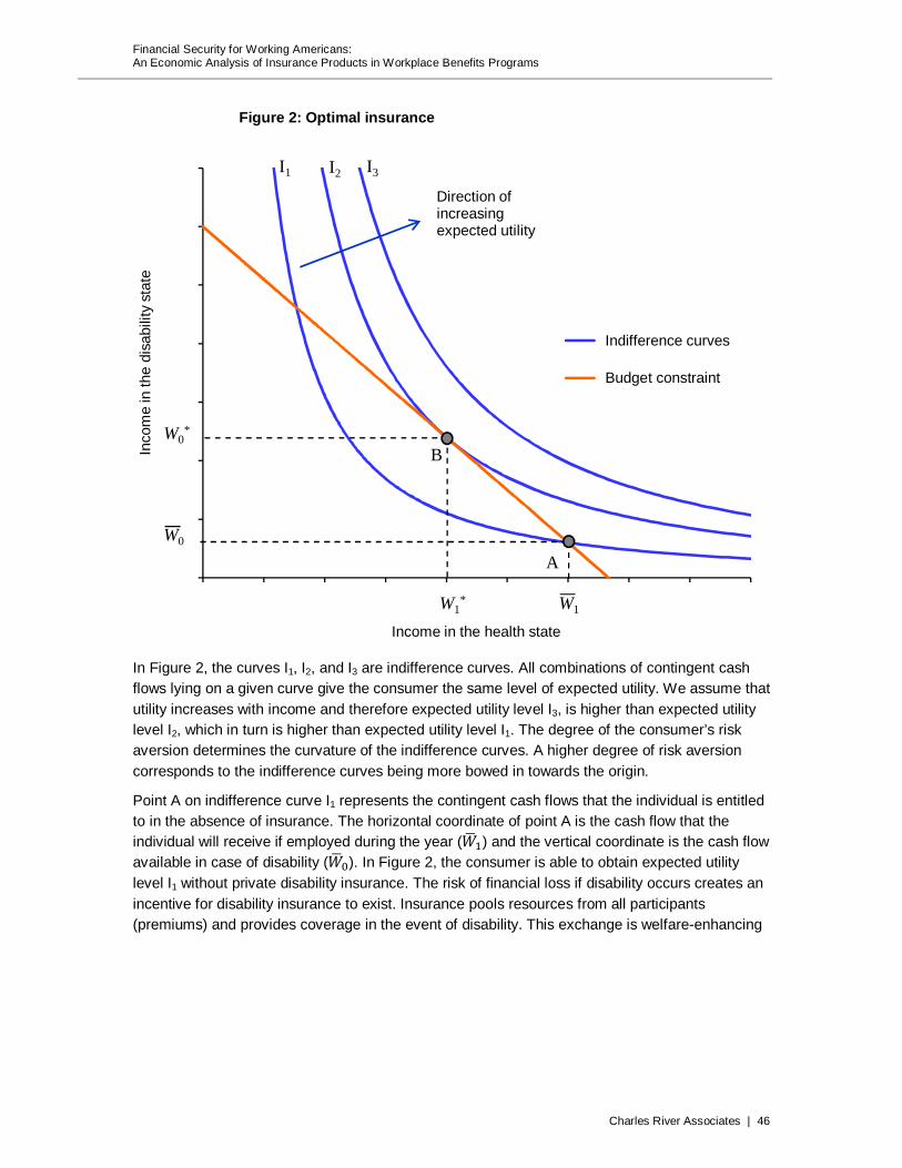
Financial Security for Working Americans: An Economic Analysis of Insurance Products in Workplace Benefits Programs
Charles River Associates | 46
Figure 2: Optimal insurance
In Figure 2, the curves I1, I2, and I3 are indifference curves. All combinations of contingent cash flows lying on a given curve give the consumer the same level of expected utility. We assume that utility increases with income and therefore expected utility level I3, is higher than expected utility level I2, which in turn is higher than expected utility level I1. The degree of the consumer’s risk aversion determines the curvature of the indifference curves. A higher degree of risk aversion corresponds to the indifference curves being more bowed in towards the origin.
Point A on indifference curve I1 represents the contingent cash flows that the individual is entitled to in the absence of insurance. The horizontal coordinate of point A is the cash flow that the individual will receive if employed during the year (푊 ) and the vertical coordinate is the cash flow available in case of disability (푊 ). In Figure 2, the consumer is able to obtain expected utility level I1 without private disability insurance. The risk of financial loss if disability occurs creates an incentive for disability insurance to exist. Insurance pools resources from all participants (premiums) and provides coverage in the event of disability. This exchange is welfare-enhancing
0
5
10
15
20
25
30
35
0 5 10 15 20 25 30 35 40 45
Inco
me
in th
e di
sabi
lity
stat
e
Income in the health state
Indifference curves
Budget constraint
A
B
W1* W1
W0*
W0
I1 I3I2
Direction of increasing expected utility
Financial Security for Working Americans: An Economic Analysis of Insurance Products in Workplace Benefits Programs
Charles River Associates | 47
in the sense that it allows risk-averse individuals to obtain a higher level of expected utility by purchasing disability insurance.3
Figure 2 demonstrates the welfare-enhancing value of private insurance by showing how the purchase of insurance allows the consumer to achieve a higher level of expected utility. The straight line crossing the horizontal and vertical axes and going through point A is the combination of contingent cash flows that can be obtained, given the endowments represented by point A and the price of insurance p given in expression (1). This line is referred to as the budget constraint. Among all combination of contingent cash flows that lie on this budget constraint, the one that maximizes expected utility (that is, the combination for which an indifference curve is tangent to the budget constraint) is the optimal combination implying the optimal amount of net insurance coverage. This optimal combination is shown as point B. Comparison of points A and B reveals that a premium 푃∗ = 푊 − 푊∗ is paid in exchange for net coverage 퐶∗ − 푃∗ = 푊∗ −푊 .
4 The amount of insurance implied by point B is, among all possible amounts the consumer
could purchase given his initial endowments and the price of insurance, the one that leads to the highest possible level of expected utility, given by I2. The existence of insurance allows consumers to move from an initial expected utility level I1 to a higher level I2.
5The degree of risk
aversion, measured by the coefficient of relative risk aversion ρ, has an influence on the amount of optimal insurance. Expression (4) shows that as ρ increases, the relationship between W0 and W1 approaches W0 = W1. In Figure 1, higher risk-aversion would be represented by an optimal insurance point B that is higher up on the budget constraint. Other things being equal (i.e., initial endowments represented by point A and the price of insurance determined by π and κ), more risk aversion leads to more insurance consumption. The relationship between the optimal insurance amount and the degree of risk aversion is due to the existence of a non-zero expense factor κ. When the expense factor is zero, the degree of risk aversion has no impact on the level of optimal insurance. Figure 3 illustrates this fact.
3 The optimal insurance point illustrated in Figure 2 is welfare enhancing because the probability of disability and the expense factor are not so high as to prevent the existence of a market for insurance. Very high disability probabilities and/or expense factors resulting in large premiums may render disability insurance unattractive. In this case, even if some individuals would be better off purchasing insurance due to high risk aversion, the market may not develop because insurance companies would not be able to sell enough policies to properly diversify their risks.
4 In Figure 2, the magnitudes of the premium paid and the net coverage obtained are roughly the same for purposes of presentation. In reality, premiums are a fraction of coverage, reflecting relatively small probabilities of loss and expense factors kept as low as possible by competitive forces. Using Equation (1), one can show that the premium per dollar of net coverage is far less than $1 per $1 of net coverage in most realistic situations. For instance, if the probability of disability is 3% per year and the expense factor is 20%, the annual premium, calculated using Equation (1), is 3.73 cents per dollar of net coverage. If the expense factor is 40%, the annual premium is 4.38 cents per dollar of net coverage.
5 At its core, the welfare-enhancing value of insurance is the result of the existence of a market for any given product. In our case, the product of interest is disability insurance. The insight that voluntary exchange facilitated by markets leads to broad welfare gains is a fundamental one in economics.

Financial Security for Working Americans: An Economic Analysis of Insurance Products in Workplace Benefits Programs
Charles River Associates | 48
Figure 3: Optimal insurance and the certainty line
When the expense factor κ is zero, Equation (4) does not involve the degree of relative risk aversion ρ and simply becomes 푊 = 푊 , shown in Figure 3 as the 45-degree line through the origin. This line is referred to as the certainty line because any point on it implies the same level of income in either state of the world. In other words, while the state of the world that will occur is uncertain, the corresponding amount of income available is not. The solution to the consumer’s maximization problem is to choose a level of coverage that implies the same net income in either state of the world. This means that optimal insurance implies that the employment income net of premium paid equals disability income plus net coverage. This situation is referred to as “full insurance.” One can say that in exchange for a premium, full insurance completely eliminates the risk of loss.
The full insurance equilibrium is shown as point C in Figure 3, where the dashed line is the budget constraint corresponding to the no-expense price, or actuarially expected claims cost, pa
6
6 The no-expense budget line is steeper that the budget line with a non-zero expense factor because pa is smaller than p. This means that a given premium can purchase a larger amount of coverage. By construction, the budget line always goes through the initial endowment point A. Also, due to the expression for expected utility, the optimal insurance point is always on the certainty line when the price of insurance is the actuarially expected claims cost.
0
5
10
15
20
25
30
35
0 5 10 15 20 25 30 35 40 45
Inco
me
in th
e di
sabi
lity
stat
e
Income in the health state
Indifference curves
Certainty line
Budget constraint
A
C
B
W1* W1
W0*
W0
I1 I3I2
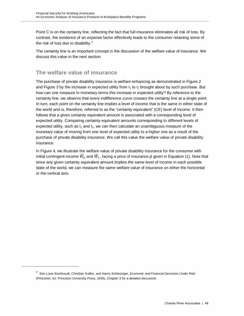
Financial Security for Working Americans: An Economic Analysis of Insurance Products in Workplace Benefits Programs
Charles River Associates | 49
Point C is on the certainty line, reflecting the fact that full insurance eliminates all risk of loss. By contrast, the existence of an expense factor effectively leads to the consumer retaining some of the risk of loss due to disability.7
The certainty line is an important concept in the discussion of the welfare value of insurance. We discuss this value in the next section.
The welfare value of insurance The purchase of private disability insurance is welfare enhancing as demonstrated in Figure 2 and Figure 3 by the increase in expected utility from I1 to I2 brought about by such purchase. But how can one measure in monetary terms this increase in expected utility? By reference to the certainty line, we observe that every indifference curve crosses the certainty line at a single point. In turn, each point on the certainty line implies a level of income that is the same in either state of the world and is, therefore, referred to as the “certainty equivalent” (CE) level of income. It then follows that a given certainty equivalent amount is associated with a corresponding level of expected utility. Comparing certainty equivalent amounts corresponding to different levels of expected utility, such as I1 and I2, we can then calculate an unambiguous measure of the monetary value of moving from one level of expected utility to a higher one as a result of the purchase of private disability insurance. We call this value the welfare value of private disability insurance.
In Figure 4, we illustrate the welfare value of private disability insurance for the consumer with initial contingent income 푊 and 푊 , facing a price of insurance p given in Equation (1). Note that since any given certainty equivalent amount implies the same level of income in each possible state of the world, we can measure the same welfare value of insurance on either the horizontal or the vertical axis.
7 See Louis Eeckhoudt, Christian Gollier, and Harris Schlesinger, Economic and Financial Decisions Under Risk (Princeton, NJ: Princeton University Press, 2005), Chapter 3 for a detailed discussion.
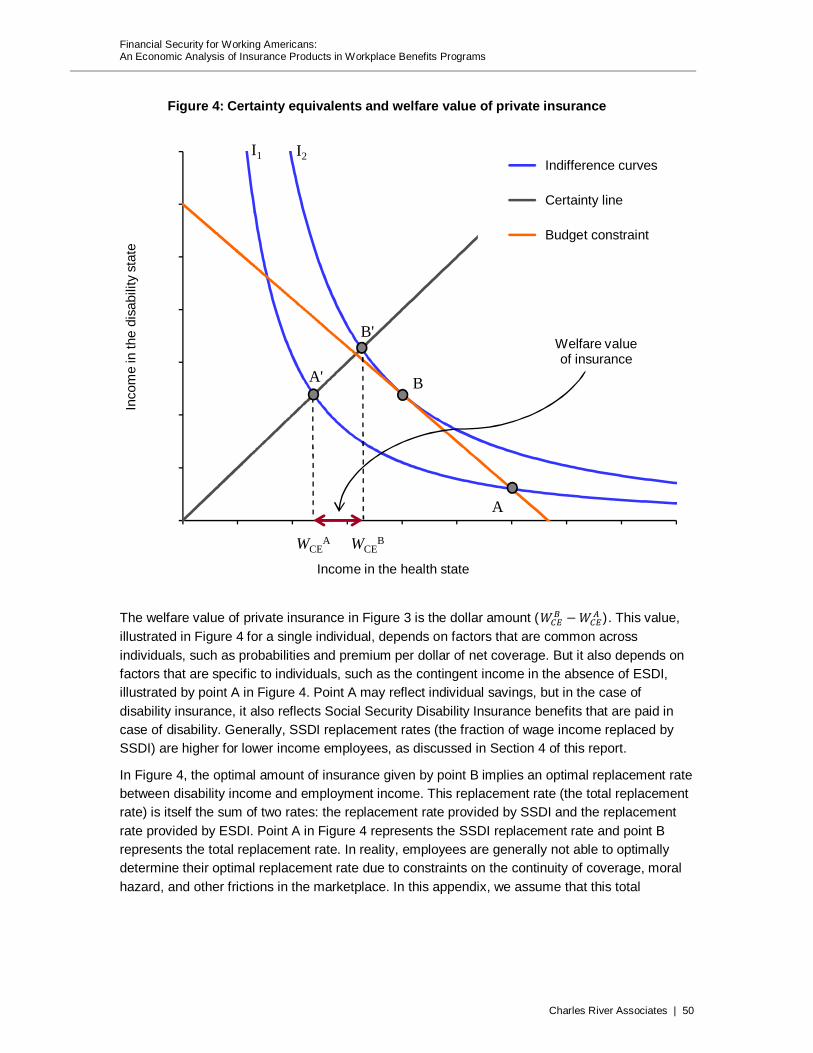
Financial Security for Working Americans: An Economic Analysis of Insurance Products in Workplace Benefits Programs
Charles River Associates | 50
Figure 4: Certainty equivalents and welfare value of private insurance
The welfare value of private insurance in Figure 3 is the dollar amount (푊 − 푊 ). This value, illustrated in Figure 4 for a single individual, depends on factors that are common across individuals, such as probabilities and premium per dollar of net coverage. But it also depends on factors that are specific to individuals, such as the contingent income in the absence of ESDI, illustrated by point A in Figure 4. Point A may reflect individual savings, but in the case of disability insurance, it also reflects Social Security Disability Insurance benefits that are paid in case of disability. Generally, SSDI replacement rates (the fraction of wage income replaced by SSDI) are higher for lower income employees, as discussed in Section 4 of this report.
In Figure 4, the optimal amount of insurance given by point B implies an optimal replacement rate between disability income and employment income. This replacement rate (the total replacement rate) is itself the sum of two rates: the replacement rate provided by SSDI and the replacement rate provided by ESDI. Point A in Figure 4 represents the SSDI replacement rate and point B represents the total replacement rate. In reality, employees are generally not able to optimally determine their optimal replacement rate due to constraints on the continuity of coverage, moral hazard, and other frictions in the marketplace. In this appendix, we assume that this total
0
5
10
15
20
25
30
35
0 5 10 15 20 25 30 35 40 45
Inco
me
in th
e di
sabi
lity
stat
e
Income in the health state
Indifference curves
Certainty line
Budget constraint
A
B'
B
WCEA WCE
B
I1 I2
A'
Welfare value of insurance

Financial Security for Working Americans: An Economic Analysis of Insurance Products in Workplace Benefits Programs
Charles River Associates | 51
replacement rate is fixed at 60%.8 This implies that, for instance, lower-level income employees who have higher SSDI replacement rates will generally be able to obtain a lower ESDI replacement rate given that the sum of these two ratios is approximately 60%.
The total replacement rate of 60% we use in this report is a pre-tax rate. Depending on how ESDI benefits are taxed, the after-tax replacement rate of a given employee could be higher than 60%, but it is hard to determine how much higher because this depends, among other factors, on the employee’s marginal tax rate and how the premium paid is split between the employee and the employer. If we were able to determine this across the distribution of employees enrolled in ESDI, we could determine the welfare value of ESDI for after-tax replacement rates.9
The model discussed in this appendix is not only applicable to disability insurance. It can also accommodate other types of insurance, such as life insurance, by reinterpreting income in the adverse state of the world. In the case of life insurance, there is no consideration of disability income and, therefore, the adverse state income level 푊 is to be interpreted as bequest for the policyholder’s beneficiary in case of death. In our calculation of the welfare value of group life insurance, we take this bequest motive into account.
8 The 60% replacement rate is generally below the optimal rate that it would obtain in a frictionless market. In Figure 3, the optimal total replacement rate that corresponds to the case with a zero expense factor is 100% (i.e., full insurance) represented by point C on the certainty line. A positive expense factor reduces the optimal total replacement rate, which in this case also depends on the degree of risk aversion. Under realistic expense factors and for relevant degrees of risk aversion, the optimal total replacement rate is well above 60%.
9 Approximately 34% of employers pay all of the disability insurance premiums, and 45% pay some of the premiums. See GenRe Research, Disability Fact Book, Sixth Edition, 2010, p. 28.
Financial Security for Working Americans: An Economic Analysis of Insurance Products in Workplace Benefits Programs
Charles River Associates | 52
Appendix B
Multi-period economic models of long-term disability insurance
Introduction The purpose of this Appendix is to investigate the benefit to society of private disability insurance programs of the sort that currently exist in the US, in addition to the public programs for such insurance. To accomplish this, we created and compared results from two economic models of disability insurance programs. MODEL 0 represents a hypothetical world with a mandatory government disability insurance program for all workers but no private market offering. MODEL 1 has the public program along with a voluntary private market program. The private market offers self-financing (actuarially neutral) disability insurance with characteristics most common to the typical employer-sponsored plans in the US, including a 20% expense margin. In MODEL 0, the worker makes no choices, and in MODEL 1, the worker chooses whether to buy private disability insurance to supplement the available government disability insurance. In this Appendix, we use “insurance” to mean only disability insurance.
Our primary measure of consumer welfare is the annual expected utility (measured in dollars) for a statistically typical (or representative) worker resulting from access to the private insurance market. We employ a new measure of cash-certainty equivalent of utility for annual consumption during a career. This consumption, in turn, is based on both:
i. scenarios of disability during working careers that we constructed through Monte Carlo simulation, and
ii. average worker salary rates from US employment survey data.
Average US salary rates for each age are used in the models. For male and female workers, this figure is $21,869 and $19,829 at age 21 and grows to $51,843 and $36,177 at age 65, respectively.1 These models assume no inflation and no income tax as well as no unemployment when not disabled.
Monte Carlo simulation is used to take into account the random elements (e.g., length of working life and both incidence and length of disability events) and the risk aversion of our typical worker. The former is based on a publicly filed disability insurance rate experience of US insurance companies. Assume our worker has constant relative risk aversion. Then comparing our metric applied to such a worker in each model tells us that the gains from access to the private disability insurance market, existing in the US, are substantial.
This gain for workers with risk aversion levels typical of the US population, varying from 4.4 to 6.6, is equivalent to a single payment at the start of their careers, ranging from $665,000 to
1 US Bureau of Labor Statistics, “Earnings by Age and Sex Third Quarter of 2009.” Retrieved from http://www.bls.gov/opub/ted/2009/ted_20091021.htm

Financial Security for Working Americans: An Economic Analysis of Insurance Products in Workplace Benefits Programs
Charles River Associates | 53
$779,000, respectively.2 We find that workers characterized by these levels of risk aversion will prefer having private insurance to supplement their mandatory government insurance coverage. In particular, workers will supplement their government insurance by purchasing the most common private disability insurance (paying benefits of 60% of wages for disabilities lasting in excess of 90 days) when faced with a choice of that or no private insurance in addition to their mandatory government insurance. Indeed, a typical worker exhibiting a risk aversion of as low as two will buy this most common private insurance, if available.
Apart from our primary measure of consumer welfare, we also examine the effect of private insurance on poverty or, more specifically, the reduction of poverty. If all workers were covered by standard employer-sponsored insurance, then poverty arising from a disability would be virtually eliminated. The proportion of workers ever in poverty during their career due to disability would fall from 7.26% to 0.23%.
For ease of explication, we will develop the notions, paradigms, and Monte Carlo simulation for the simpler MODEL 0 first and defer addressing the more complex MODEL 1 until Section 5.
1. Basic conventions and notation The two economic models we construct will be described through the prism of our single representative worker and will be based on that worker’s consumption in each year of his or her career. The models assume that a worker’s career starts at the beginning of some calendar year, which also happens to be that worker’s Nth birthday, and ends on the last day of some subsequent calendar year, either at death or retirement (on the day before their Mth birthday if still alive). Years are indexed by 푡, and our worker’s last working year is labeled with the integer 푸. The first year of the worker’s career is calendar year 푡 = 1, which starts at 퐷푎푡푒 and ends a year later at 퐷푎푡푒 . Similarly, every career year 푡 for 푡 = 1,2,3, … , 푄 starts on 퐷푎푡푒 and ends on 퐷푎푡푒 .
Assume all dollar amounts are in real dollars and that there is no inflation or income tax. Money is exchanged only at yearend for computational tractability. That is, only at a yearend 푡 (i.e., at 퐷푎푡푒 for each 푡 = 1,2,3, … , 푄), does a worker ever:
i. receive any wages 푺풕 and/or disability benefits 푩풕 due,
ii. pay any disability premiums 품풑풓풆풕 due,
iii. deposit savings 푺푨푽풕 or withdraw savings 푫푰푺푺푨푽풕,
iv. spend on consumption 푪풕, and/or
v. retire or die on 푫풂풕풆푸.
Disability events can start on any Date within a career year 푡 (not necessarily at yearend) for
2 The estimates of average risk aversion in the US population are given by S.D. Hanna and S. Lindamood, in “An Improved Measure of Risk Aversion,” Financial Counseling and Planning, 15(2) (2004), pp. 27–38; R.B. Barsky, F.T. Juster, M.S. Kimball, and M.D. Shapiro, “Preference parameters and behavioral heterogeneity: An experimental approach in the Health and Retirement Study,” Quarterly Journal of Economics, 112 (2) (1997), pp. 537–579; and S.D. Hanna, M.S. Gutter, and J.X. Fan, “A measure of risk tolerance based on economic theory,” Financial Counseling and Planning, 12 (2) (2001), pp. 53–60. Barsky et al. provided a mode of 5.65, and the other two studies provided the upper and lower bounds.
Financial Security for Working Americans: An Economic Analysis of Insurance Products in Workplace Benefits Programs
Charles River Associates | 54
푡 = 0,1,2,3, … , (푄 − 1), and can end at any subsequent yearend 퐷푎푡푒 for 푘 = 푡, 푇 + 1, … , 푄. Disability is not allowed after 퐷푎푡푒 as the worker has retired from the workforce. Our primary measure of consumer welfare is the present value of a cash certainty equivalent of our worker’s expected utility for consumption each year. That expected utility is computed over 100,000 Monte Carlo scenarios (or paths) of the cash flow available to our worker for consumption on each 퐷푎푡푒 via (i) to (v) above.
The existence of disability, which determines the 푆 and 퐵 in (i) to (v) above for each year 푡, depends on the outcome of a four-stage compound draw described in Section 2. Our representative worker enters this compound draw in each calendar year of his or her working life where he or she is not disabled form a previous disability event. Our results derive from the consumption patterns among 100,000 such working lives in a Monte Carlo simulation based on those compound draws.
2. Mortality and disability of the worker
2.1. Stage 0 Draw at 퐷푎푡푒 : gender and 푄–year working life
The gender of each representative worker is designated along with a 푄-year working life at the start of his or her career on 퐷푎푡푒 . We call these drawings the STAGE 0 DRAW. Its probability distribution is developed from the 2006 Social Security survival table web page found at http://www.ssa.gov/OACT/STATS/table4c6.html. We distinguish between males and females since they are separately tracked in the survival table. A draw at the initiation of the process on each 퐷푎푡푒 , with 50% probability to each gender, provides the worker’s gender for assigning both a salary and the various disability draws.3 These are the key inputs to the Monte Carlo simulation, which is used to determine the worker’s consumption 퐶 each year 푡.
The models assume that 퐷푎푡푒 is the worker’s 21st birthday and that he or she will retire at age 65, if alive then. We call the maximum 푡 value in the worker’s career 푸풎풂풙 = 65 − 21 = 44. The Social Security survival source table provides the probability of dying at each yearend 푡 (each age from 22 to 65), for each gender, conditional upon survival up to yearend 푡 − 1. This is translated into a probability of our worker dying at each career yearend on 퐷푎푡푒 . 푄 is drawn from the distribution of these translated probabilities. The worker never knows the value of 푄 drawn.
2.2. Stage 1 Draw: disability event in each year t
Once 푄 is chosen in the STAGE 0 DRAW of Subsection 2.1, we proceed to construct a working/disability scenario over the worker’s 푄-year career. This scenario is a vector 푾 = 푊 , 푊 , 푊 , … , 푊 , where each 푾풕 is the proportion of year 푡 that this worker was not disabled. It is constructed from a four-stage compound draw at the start of certain years 푡 (i.e., on
3 We recognize that the working population is not always evenly balanced between males and females but varies over time and by age. However, for our purposes of a first approximation of social welfare gain from private insurance, we have not refined our measures, although both of our models accommodate any patterns over time and by age.
Financial Security for Working Americans: An Economic Analysis of Insurance Products in Workplace Benefits Programs
Charles River Associates | 55
certain 퐷푎푡푒 ). This process always starts with the first set of the STAGE 1 DRAWS on 퐷푎푡푒 (i.e., at the beginning of year 1). It is repeated at the beginning (on 퐷푎푡푒 ) of each subsequent year that the worker enters the draws as described below (whenever he or she is not disabled past such 퐷푎푡푒 from a previous disability event). Formally, for any positive integer number of years k, for which a prior disability event drawn on a previous 퐷푎푡푒 continues (i.e., there is such a positive integer k such that 퐷 > 푗 − 1 + 푘), the worker does not enter the STAGE 2 to STAGE 4 DRAWS on 퐷푎푡푒 . The last possible set of draws is on 퐷푎푡푒 . The outcome of this draw is either a disability event, labeled 푯풕 = 1, or not, labeled 푯풕 = 0.
On 퐷푎푡푒 for 푡 = 1,2,3, … , 푄 − 1, the worker enters the disability draw for year 푡 with probability 푷풕 of a disability event, which is separate from any consideration of the length 푫풕 of disability that may start on year t. If this draw yields no disability event, then we say 퐻 = 0, 퐷 = 0, and the worker
i. works for all of year 푡 (i.e., 푊 = 1),
ii. skips STAGE 2, STAGE 3, and STAGE DRAWS at 퐷푎푡푒 , and
iii. participates in the next STAGE 1 DRAW on 퐷푎푡푒 .
Otherwise, the worker has a disability event on 퐷푎푡푒 , we say 퐻 = 1, and the worker immediately enters STAGE 2 and STAGE 3 DRAWS to determine the value of 퐷 and a component of benefit computations on 퐷푎푡푒 .
The probability 흅풕 of a disability event at any such start of a calendar year 푡 is based on advance private actuarial data received from Rick Leavitt, a pricing and consulting actuary with the Smith Group. Those data are from publically filed GLTD Incidence Rates that reflect the average reported incidence and rates for individuals insured with 90-day elimination periods (initial disability period before disability coverage begins) from the disability claims filed with MetLife, Sun, Guardian, and Principal insurance companies.4
2.3. Stage 2 Draw: length of disability event
The length 푫풕 of any disability event is drawn from a uniform probability density function 풇풕(푫풕), over the various intervals in the Experience Tables that accompanied the GLTD 2008 Incidence Rates described in Subsection 2.2. 퐷 is a real number on those intervals of time. 푓 (퐷 ) is based on long-term disability claim survivorship in those tables, which has the following characteristics:
(a.) Includes only claims with a 90-day and 180-day elimination period and assumes lifetime benefit duration for all claims (i.e., a disability event lasting beyond retirement is insured). Note: we corrected for disability duration lasting past age M, which we do not allow in our two models.
(b.) Benefit amounts, claim diagnosis, and definitions of disability match the mix of workers in the insured pools included in that 2008 study.
2.4. Start and end of disability period
4 These incident rates were compiled from manual rate filings submitted to North Carolina by Guardian (6/2008), MetLife (9/2008), and Principal (6/2010), and to Florida by SunLife (5/2009).

Financial Security for Working Americans: An Economic Analysis of Insurance Products in Workplace Benefits Programs
Charles River Associates | 56
The models adopt the following convention for the start and end dates of any disability event with duration 퐷 that was drawn on 퐷푎푡푒 in STAGE 1. 푫풅풐풘풏풕 and 푫풖풑풕 are defined as the smallest and largest integers that are not smaller and not larger, respectively, than 퐷 . This disability event starts the fraction 퐷푢푝 – 퐷 of a year after 퐷 (i.e., it starts during year t) and ends 퐷푢푝 years after 퐷푎푡푒 . Note these two fractions are 0 if 퐷 is an integer.
The disabled worker does not work for 퐷 years after the disability event that starts during year 푡 (between 퐷푎푡푒 and 퐷푎푡푒 ). Nor does the worker participate in any draws while disabled (e.g., the worker does not draw on any 퐷푎푡푒 for any integer k such that 푡 − 1 < 푘 < 푡 − 1 + 퐷 ). We assume that each of the 휋 and 푓 is independent of all the others and will refer to the 푄-vector of their probabilities and distributions as 휋 = 휋1, 휋2, 휋3, … , 휋푄 and 푓 = 푓 , 푓 , 푓 , … , 푓 , respectively. To the extent that a worker with higher cumulative prior disability has a higher future probability of disability and/or longer duration than a worker with a lower such cumulative prior disability, this modeling understates the social welfare gains from access to the private insurance market. This follows from the risk aversion of our worker and Jensen’s inequality.
2.5. Stage 3 Draw: government claim denied or not
The probabilities of disability 휋 and the density functions of its duration 푓 in Subsection 2.3 are taken from private insurance company historical data and thus reflect disabilities as defined and paid by such companies. The Social Security Administration and administrators for state disability insurers do deny claims that are accepted and paid by private insurers. We take the private insurance company data as the baseline disability for our model and add yet another draw to determine if such disabled workers are denied government benefits in determining our worker’s cash flow in MODEL 0. From the Social Security Administration data on the denial rate of claims, we have probability 풑풓풐풃풙 that the worker’s disability event will have his claim denied. We set 푝푟표푏푥 = 0.5, roughly consistent with an average two-year waiting period discussed immediately below. If the worker draws a denial we set 푋 = 1, and if not we set 푋 = 0.
2.6. Social Security eligibility period and delay of payments owed
In the US there is a Social Security Administration minimum disability duration 풇풎풅풅 = 1 year. Only if the STAGE 2 draw provides 퐷 ≥ 푓푚푑푑 is the worker entitled to federal government disability benefits from the Social Security Administration. But these benefits are often denied and always delayed. Any Social Security disability benefits due, for disability during the initial 푔푤푎푖푡 years of disability, are not payable until 푔푤푎푖푡 years after the start of the disability. We set this benefit parameter 품풘풂풊풕 = 0.5 years in order to conform with current Social Security rules.
Distinct from this 푔푤푎푖푡, there is an average delay of 품풅풆풍풂풚 years from the time that benefits, which are eventually paid, were first payable (which is already after the 푔푤푎푖푡 delay) to their actual payment. This means, on average, the first 푔푑푒푙푎푦 years of benefits payments due are paid all at once 푔푑푒푙푎푦 years late. A table of Social Security rates for workers not yet receiving a Social Security disability benefit, but who have received private disability benefits, is used to estimate this parameter. We set 푔푑푒푙푎푦 equal to the average period of time that private disability claims for disabilities, of at least one year, are paid but for which the Social Security Administration has not paid. This is adjusted for the difference between the typical 90-day elimination period of private insurance and the 푔푤푎푖푡 of the Social Security Administration.
It turns out that a large part of the social welfare gain from access to the private disability
Financial Security for Working Americans: An Economic Analysis of Insurance Products in Workplace Benefits Programs
Charles River Associates | 57
insurance market is attributable to the delay in benefits paid. If 퐷 < 푓푚푑푑, then the worker receives no federal disability benefits but may receive disability benefits from the state, territory, or the District of Columbia where the worker is employed. We call these jurisdictions “states” and their disability benefits “state benefits.”
2.7. Stage 4 Draw: work-related or not
This draw determines whether the cause of the disability event is work related or not. There is probability 풘풓풆풍 that it is work related and probability (1 − 푤푘푟푒푙) that it is not, where 0 <푤푘푟푒푙 ≤ 1. STAGE 2 and STAGE 3 DRAWS occur at the same time as the STAGE 1 draw on 퐷푎푡푒 . We set 푤푘푟푒푙 = 0.10.5
If the disability is work related, then the worker receives state benefits (in the US this is called workers’ compensation) up to the state-prescribed maximum period of disability benefit payments. We assume the rate of such state benefits per year of disability equals that of the federal benefits modeled below, but state benefits offset any federal benefits eventually paid for the same disability period of time. Thus, the total of federal and state benefits in MODEL 0 and MODEL 1 equals the federal benefits amounts/year modeled below. Furthermore, we ignore the disutility and benefits associated with compensation for medical costs incurred from the disability. This ignoring of the uncertainty in the timing of such medical benefits understates the social welfare of private insurance because of worker risk aversion and Jensen’s inequality.
If the disability is not work related, then the worker receives no state benefits. Thus a worker's disability, of less than 푓푚푑푑 (which currently is 퐷 < 1) from a cause that is not work related, does not entitle the worker to any federal or state disability benefits. Note that most states in the US have workers’ compensation programs that can, or must, be underwritten by private insurance companies with benefits set by the state. However, we model these state benefits as part of government disability insurance.
2.8. Results of Stages 1 to 4
Given a 푄 value and a gender from the STAGE 0 draw for our representative worker, the implementation of our sequence of compound draws is straightforward and is not elaborated here. The result of one set of 푄 number and the STAGE 1 to STAGE 4 draws is a scenario of disabilities for that one worker. It is handy to have a notation for the proportion of each year 푡 that the worker is disabled, such as 풀풕. The 푌-vector of proportions of each calendar year that the worker is disabled is 푌 = 푌 , 푌 , 푌 , … , 푌 for a particular Monte Carlo scenario, where 푌 = 1 – 푊 for 푡 = 1,2,3, … , 푄.
Here we summarize this set of compound draws. For any 퐷푎푡푒 on which no prior disability event continues, the worker enters the STAGE 1 DRAW. If that draw is 퐻 = 0, we have no disability that year, 푊 = 1, 푌 = 0, and we are done with the compound draw for year 푡 (i.e., the draws at 퐷푎푡푒 ). Otherwise 퐻 = 1, and the worker enters the STAGE 2 to STAGE 4 DRAWS on that date. STAGE 2 provides a 퐷 value; STAGE 3 either federal benefit denial 푋 = 1 or not 푋 = 0; and
5 This is consistent with the information that 90% of disabilities are not caused by work-related injuries or conditions, as reported by the National Safety Council in Injury Facts, 2008 edition.

Financial Security for Working Americans: An Economic Analysis of Insurance Products in Workplace Benefits Programs
Charles River Associates | 58
STAGE 4 either the disability event is work related 푤푘푟푒푙 = 1 or not 푤푘푟푒푙 = 0. If 퐷 < 1 or 푋 = 1, the worker receives no federal benefits, otherwise he or she receives federal benefits. Regardless, if 푤푘푟푒푙 = 1, the worker receives state benefits that offset any federal benefits that might be received for the same disability period. Otherwise, he or she receives no state benefits. Note, we set: 푊 = 1 if 퐷 = 0, 푊 = 0 if 퐷 ≥ 1, and 푊 = 퐷 if 퐷 < 1. Furthermore, if for some positive integer 푘 we have, 퐷 ≥ 푘, then we set 푌 = 1 and 푊 = 0 for 푖 =1,2,3, . . , 푘. The main purpose of the Monte Carlo simulation is to create 100,000 work scenarios 푊 = 푊 , 푊 , 푊 , … , 푊 .
3. Worker cash flow and consumption in MODEL 0: mandatory government insurance only
For each of the 100,000 sets of Monte Carlo STAGE 1 to STAGE 4 DRAWS for our worker, specified in Subsections 2.2 to 2.5 above, there are the following components of that worker’s cash flow each year, and that net cash flow is his or her consumption in that year:
3.1. Salary
As noted in Subsection 2.1, the gender of the individual worker is designated in STAGE 0 along with working life 푄. Our worker earns wages 푆 per year for whatever fraction 푊 of a year that he or she is not disabled in each working year 푡 = 1,2,3, … , 푄. The worker’s gender and annual salary rate 푠 for each year 푡 are taken from the data described in the Introduction. The worker’s wages earned for each year 푡 are thus 푆 = 푠 푊 , which are paid on 퐷푎푡푒 .
3.2. Government insurance premium
On Date the worker pays mandatory government disability insurance premium 품풑풓풆풕, where 푔푝푟푒 = 푔 MIN{푆 , 푔푐푎푝}. These parameters, 품 and 품풄풂풑, chosen by the government disability insurance administration to be actuarially neutral (at least as a policy), i.e., self-financing, in conjunction with their choice of premium parameters, and the administrative cost (as a proportion of benefits paid) gload they will face in Subsection 3.6. The current (2011) values are 푔 = 0.104 (sum of worker and employer rates) and 푔푐푎푝 = $106,800.6
We use this sum of rates to capture the social welfare cost and to be comparable with unsubsidized private insurance. If the government charges too little or too much to be just self-financing, it is a cost or benefit to the government (and thus society) that offsets to members of society on average at least. If employers mischarge, it is a cost or benefit of employing a worker that lowers or raises wages of such workers in a competitive labor market.
6 The Social Security withholding tax is generally 6.2% of the employee’s gross wage amount with the employer paying another 6.2% of that amount for a total of 12.4% up to the Social Security Wage Base, which is $106,800 for 2009 through 2011. In 2011, the employee portion of the Social Security withholding tax is reduced to 4.2%, so the total is 10.4%. This tax funds both the Disability Income and the Old Age and Survivors trust funds of Social Security. See http://www.socialsecurity.gov/OACT/ProgData/taxRates.html.
Financial Security for Working Americans: An Economic Analysis of Insurance Products in Workplace Benefits Programs
Charles River Associates | 59
3.3. Savings
On 퐷푎푡푒 the worker saves nonnegative proportion 풔풂풗풑풓풐 of any wages 푆 that the worker earns for year 푡 in excess of the disability premium 푔푝푟푒 paid for year 푡. The amount of the worker’s year 푡 marginal savings is thus 푆퐴푉 = 푠푎푣푝푟표 (푆 − 푔푝푟푒 ). We call it “rainy day savings” because it is distinct from any retirement savings. His or her accumulated rainy day savings on 퐷푎푡푒 is 푨푪푺푨푽풕, and this is net of any previous or current dissaving. The amount of dissaving in any year 푡 will be specified in Subsection 3.7.
퐴퐶푆퐴푉 = (푆퐴푉 − 퐷퐼푆푆퐴푉 )
3.4. Government benefit eligibility
Consider a worker’s disability event that starts in year 푡 (drawn on 퐷푎푡푒 ), with:
i. duration 퐷 , according to a set of STAGE 0, STAGE 1, and STAGE 2 DRAWS,
ii. that was not denied in a STAGE 3 DRAW, and
iii. either 푤푟푒푙 value according to a STAGE 4 DRAW.
This worker receives disability benefit 퐵 ≥ 0 paid on certain Date for 푘 ≥ 푡, according to which of the three mutually exclusive and exhaustive cases, listed below, are satisfied by 퐷 , 푋 , and 푤푟푒푙. These cases hinge on whether:
a. 퐷 < 푓푚푑푑 or not, where 푓푚푑푑 is the minimum disability period that can qualify for federal government disability benefits;
b. the disability claim is denied or not (whether 푋 = 1 or = 0)
c. the disability cause was work related or not (whether 푤푟푒푙 = 1 or 0). Let 푓푚푑푑푢푝 be the smallest integer not less than 푓푚푑푑, and recall from Subsection 2.6 that 퐷푢푝 is the smallest integer not smaller than 퐷 . The four Government Benefit Eligibility Cases are as follows:
Government benefits are owed for disability events occurring in and only in:
CASE 1 year (푡 + 푘) for 푘 = 0,1,2, … , 퐷푢푝 if STAGE 4 draws 푤푘푟푒푙 = 1. CASE 2: year (푡 + 푘) for k = 푓푚푑푑푢푝, 푓푚푑푑푢푝 + 1, 푓푚푑푑푢푝 + 2, … , 퐷푢푝푡
if STAGE 2 draws 퐷 ≥ 푓푚푑푑, STAGE 3 draws 푋 = 0, and STAGE 4 draws 푤푘푟푒푙 = 0
CASE 3: no year if STAGE 2 draws 퐷 < 푓푚푑푑 or STAGE 3 draws 푋 = 1, and STAGE 4 draws 푤푘푟푒푙 = 0.
Note in Case 1 that Social Security pays part of those benefits (in addition to the state insurance) only if 퐷 ≥ 푓푚푑푑 and 푋 = 1, but any state benefits received for disability in the overlapping CASE 2 years must be rebated to Social Security. Thus, the total government benefits in Case 1
Financial Security for Working Americans: An Economic Analysis of Insurance Products in Workplace Benefits Programs
Charles River Associates | 60
are the same regardless of the 퐷 and 푋 values. Recall in Subsection 2.7 that we set state benefits equal to Social Security benefits in amount, but that: (i) they have different eligibility requirements, (ii) are paid with 푔푤푎푖푡 = 0 = 푔푑푒푙푎푦, and (iii) any state benefits overlapped by Social Security benefits are deducted from the latter. Thus, there is no need to distinguish in our models between state and Social Security benefits in terms of payment amounts for any period of disability that is covered by either.
3.5. Government benefits amounts paid each year
Suppose our worker is entitled to some benefits for a given period of disability 푌 that occurs in year 푡, according to Subsection 3.4. Then the amount of benefits due to be paid 퐵푂 as a result of 푌 , is determined as follows. For 푗 = 1,2,3, we express 퐵푂 in terms of:
i. proportions 풔풔풋 of that part of salary which would have been earned while he or she is disabled in year t (i.e., 푠푠 proportion of 푌 푠 ), and
ii. income levels 풃풆풏풅풋, which is the amount of 푌 푆 at which these rates change,
where 0 < 푠푠 ≤ 1 and 푏푒푛푑 > 0.
Social Security benefits owed for disability during year 푡 are 퐵푂 are:
a. 풔풔ퟏ proportion of any 푆 up to 푏푒푛푑 amount of 푆 , plus
b. 풔풔ퟐ proportion of any 푆 from 푏푒푛푑 to 푏푒푛푑 amounts, plus
c. 풔풔ퟑ proportion of any 푆 from 푏푒푛푑 to 푏푒푛푑 amounts, and
d. Zero proportion of any 푆 above 푏푒푛푑 amount.
We write this mathematically to conform, to the current Social Security Administration rules, as
퐵푂 = ss MAX 0, 푀퐼푁 푆 − 푏푒푛푑 , 푏푒푛푑 − 푏푒푛푑 ,
where 푠푠 = 0.90, 푠푠 = 0.35, 푠푠 = 0.15, 푏푒푛푑 = $0, 푏푒푛푑 = $9,132, 푏푒푛푑 = $55,032, and 푏푒푛푑 = $106,800.
3.6. Delay of government benefit payment
Our Monte Carlo simulation allows us to model the delay in the payment of Social Security benefits due (for 푔푑푒푙푎푦 years) that was described in Subsection 2.6. Since our models pay only at yearends, we introduce 푔푑푒푙푎푦푢푝 as the smallest integer not less than 푔푑푒푙푎푦. This delay is implemented in our models, or not, by setting the switch 푠푤 to 1 or to 0, respectively. We define the benefits paid 퐵 to our worker as a function of the 퐵푂 stemming from a disability event in year 푡 as:
퐵 = (1 − 푠푤) 퐵푂 for 푘 = 0,1,2, … , 푔푑푒푙푎푦푢푝 − 1,
= 퐵푂푡+푘 + 푠푤 퐵푂푡 + 퐵푂푡+1 + ⋯ + 퐵푂푡+(푘−1) for 푘 = 푔푑푒푙푎푦푢푝, and
= 퐵푂 for 푘 > 푔푑푒푙푎푦푢푝.

Financial Security for Working Americans: An Economic Analysis of Insurance Products in Workplace Benefits Programs
Charles River Associates | 61
These parameters in Subsections 3.4, 3.5, and this subsection are chosen, in conjunction with their choice of 푔 and 푔푐푎푝 in Subsection 3.2, to make the insurance program, including the administrative cost, self-financing. By self-financing we mean that the present value of the premiums collected equal the present value of the benefits paid plus an administrative “load” that we label 품풍풐풂풅. This is true over the average career of the 100,000 representative workers in our Monte Carlo simulation. Thus, it holds for any change of age distribution in the insured population and does not depend on a steady state of age cohorts that would be the case if we computed it for any particular distribution of age cohorts. It does depend on the stability of 푓 and 휋.
More particularly, let 푔푙표푎푑 be the total cost (apart from benefits paid) of the government disability insurance administration as a proportion of the total benefits paid out each year. For our models, 푔푙표푎푑 = 0.2 because that approximates the private disability insurance company average expense margin, and the Social Security Administration is likely not significantly more efficient than that average. We assume 푔푙표푎푑 is constant over time. Given the government’s choice of benefit parameters above, that is, 푔푐푎푝 = $106,800, and our 푔푙표푎푑 = 0.2, we set 푔 by trial and error, so that the expected present value in our Monte Carlo simulation of the benefit cost (associated with the (1 + 푔푙표푎푑) ∑ 퐵 (1 + 푅푔) ) equals the expected present value of the disability premiums 푔푝푟푒 collected, given a government discount factor 푅푔. We set 푅푔 =.02.
3.7 Dissavings
Workers dissave only in years in which they have a disability event and at retirement or death. Consider a given year 푡 when our worker has a disability event. In such year, the worker dissaves in an effort to maintain part of their full-year-employment consumption level. Such year 푡 dissaving is 푞 proportion of this gap: (a) what consumption would have been with no disability event, minus (b) what it would have been with the disability in the absence of dissaving. Note (a) is just (1 − 푔푟푝푒) 푠 . But the subtler (b) is the worker’s year t consumption from:
b.1 wages received during the 푊 portion of year 푡, if any, in which the worker is not disabled (net of any disability premiums paid and savings from those wages), plus
b.2. any disability benefits 퐵 received in year 푡.
We specify that a worker with any disability event in year 푡 dissaves on 퐷푎푡푒 this amount:
DISSAV = MIN{ACSAV , 푞[(1 − 푠푎푣푝푟표)(1 − 푔푝푟푒) 푠 − (푆 − 푔푝푟푒 + 퐵 )]}
where 0 ≤ 푞 ≤ 1. We set 푞 = 0.5. Recall 퐴퐶푆퐴푉 is defined in Subsection 3.3 and we write 푠 to mean a full year of wages in year 푡.
3.8. Consumption
At the end of each career year 푡 before the year of retirement or death, our worker consumes
퐶 = MIN{ 푀푖푛푐표푛, 푆 − 푆퐴푉 + 퐷퐼푆푆퐴푉 + 퐵 } on Date for all 푡 = 1,2,3, … , 푄 − 1.
At retirement or death on 퐷푎푡푒 , our worker consumes
퐶 = MIN 푀푖푛푐표푛, 푆 − 푆퐴푉 + 퐷퐼푆푆퐴푉 + 퐵 + 퐴퐶푆퐴푉 .
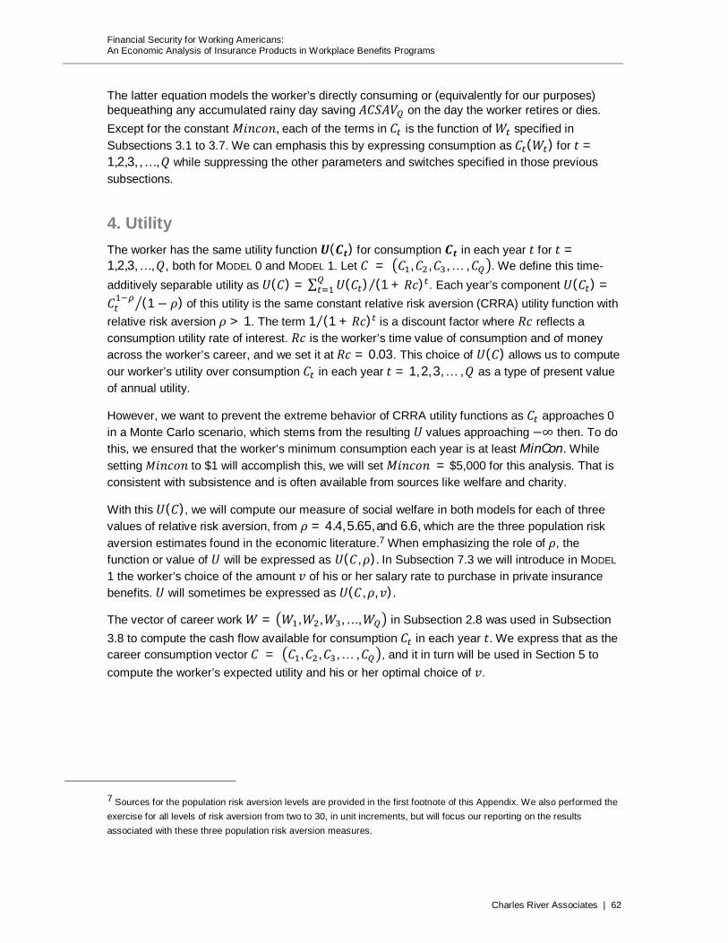
Financial Security for Working Americans: An Economic Analysis of Insurance Products in Workplace Benefits Programs
Charles River Associates | 62
The latter equation models the worker’s directly consuming or (equivalently for our purposes) bequeathing any accumulated rainy day saving 퐴퐶푆퐴푉 on the day the worker retires or dies. Except for the constant 푀푖푛푐표푛, each of the terms in 퐶 is the function of 푊 specified in Subsections 3.1 to 3.7. We can emphasis this by expressing consumption as 퐶 (푊 ) for 푡 =1,2,3, , … , 푄 while suppressing the other parameters and switches specified in those previous subsections.
4. Utility
The worker has the same utility function 푼(푪풕) for consumption 푪풕 in each year 푡 for 푡 =1,2,3, … , 푄, both for MODEL 0 and MODEL 1. Let 퐶 = 퐶 , 퐶 , 퐶 , … , 퐶 . We define this time-additively separable utility as 푈(퐶) = ∑ 푈(퐶 ) (1 + 푅푐)⁄ . Each year’s component 푈(퐶 ) =퐶 (1 − 휌) of this utility is the same constant relative risk aversion (CRRA) utility function with relative risk aversion 휌 > 1. The term 1 (1 + 푅푐)⁄ is a discount factor where 푅푐 reflects a consumption utility rate of interest. 푅푐 is the worker’s time value of consumption and of money across the worker’s career, and we set it at 푅푐 = 0.03. This choice of 푈(퐶) allows us to compute our worker’s utility over consumption 퐶 in each year 푡 = 1, 2, 3, … , 푄 as a type of present value of annual utility.
However, we want to prevent the extreme behavior of CRRA utility functions as 퐶 approaches 0 in a Monte Carlo scenario, which stems from the resulting 푈 values approaching −∞ then. To do this, we ensured that the worker’s minimum consumption each year is at least MinCon. While setting 푀푖푛푐표푛 to $1 will accomplish this, we will set 푀푖푛푐표푛 = $5,000 for this analysis. That is consistent with subsistence and is often available from sources like welfare and charity.
With this 푈(퐶), we will compute our measure of social welfare in both models for each of three values of relative risk aversion, from 휌 = 4.4, 5.65, and 6.6, which are the three population risk aversion estimates found in the economic literature.7 When emphasizing the role of 휌, the function or value of 푈 will be expressed as 푈(퐶, 휌). In Subsection 7.3 we will introduce in MODEL 1 the worker’s choice of the amount 푣 of his or her salary rate to purchase in private insurance benefits. 푈 will sometimes be expressed as 푈(퐶, 휌, 푣).
The vector of career work 푊 = 푊 , 푊 , 푊 , … , 푊 in Subsection 2.8 was used in Subsection 3.8 to compute the cash flow available for consumption 퐶 in each year 푡. We express that as the career consumption vector 퐶 = 퐶 , 퐶 , 퐶 , … , 퐶 , and it in turn will be used in Section 5 to compute the worker’s expected utility and his or her optimal choice of 푣.
7 Sources for the population risk aversion levels are provided in the first footnote of this Appendix. We also performed the exercise for all levels of risk aversion from two to 30, in unit increments, but will focus our reporting on the results associated with these three population risk aversion measures.
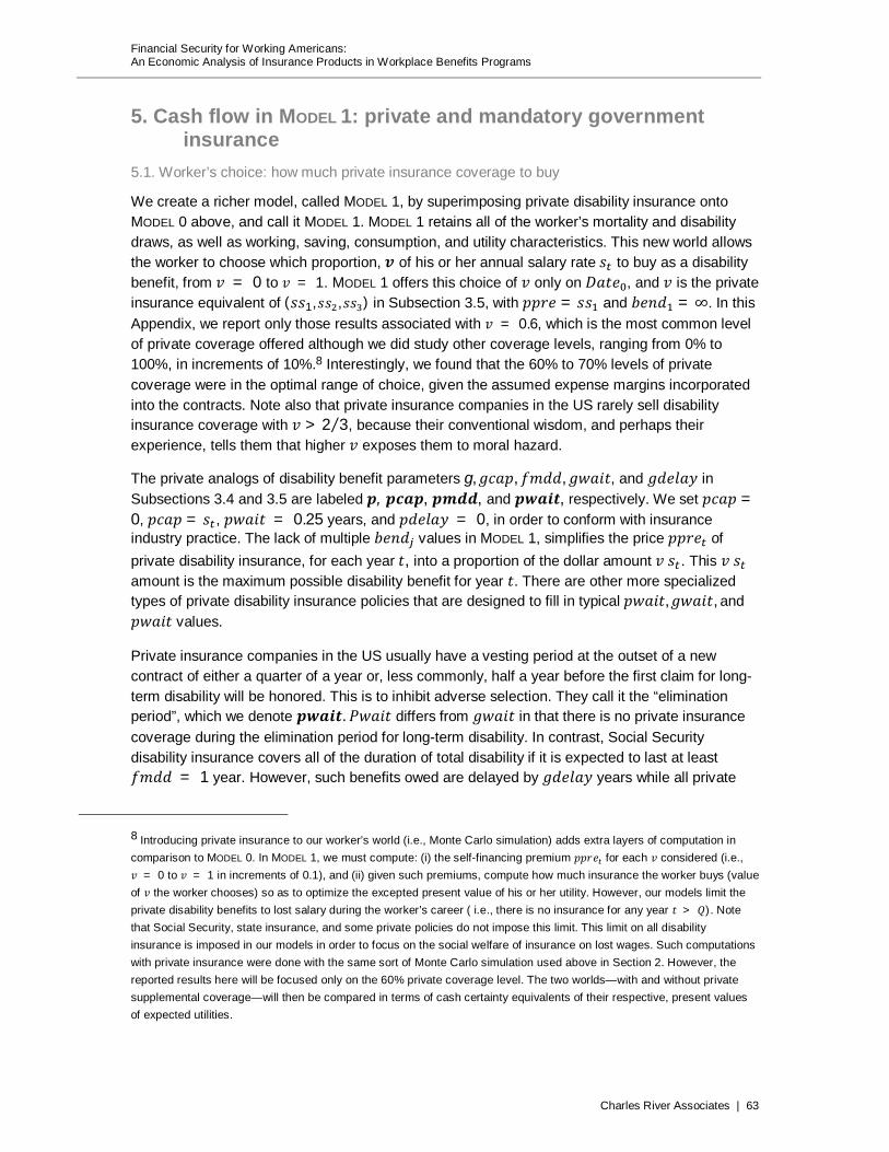
Financial Security for Working Americans: An Economic Analysis of Insurance Products in Workplace Benefits Programs
Charles River Associates | 63
5. Cash flow in MODEL 1: private and mandatory government insurance
5.1. Worker’s choice: how much private insurance coverage to buy
We create a richer model, called MODEL 1, by superimposing private disability insurance onto MODEL 0 above, and call it MODEL 1. MODEL 1 retains all of the worker’s mortality and disability draws, as well as working, saving, consumption, and utility characteristics. This new world allows the worker to choose which proportion, 풗 of his or her annual salary rate 푠 to buy as a disability benefit, from 푣 = 0 to 푣 = 1. MODEL 1 offers this choice of 푣 only on 퐷푎푡푒 , and 푣 is the private insurance equivalent of (푠푠1, 푠푠 , 푠푠 ) in Subsection 3.5, with 푝푝푟푒 = 푠푠 and 푏푒푛푑 = ∞. In this Appendix, we report only those results associated with 푣 = 0.6, which is the most common level of private coverage offered although we did study other coverage levels, ranging from 0% to 100%, in increments of 10%.8 Interestingly, we found that the 60% to 70% levels of private coverage were in the optimal range of choice, given the assumed expense margins incorporated into the contracts. Note also that private insurance companies in the US rarely sell disability insurance coverage with 푣 > 2 3⁄ , because their conventional wisdom, and perhaps their experience, tells them that higher 푣 exposes them to moral hazard.
The private analogs of disability benefit parameters g, 푔푐푎푝, 푓푚푑푑, 푔푤푎푖푡, and 푔푑푒푙푎푦 in Subsections 3.4 and 3.5 are labeled 풑, 풑풄풂풑, 풑풎풅풅, and 풑풘풂풊풕, respectively. We set 푝푐푎푝 =0, 푝푐푎푝 = 푠 , 푝푤푎푖푡 = 0.25 years, and 푝푑푒푙푎푦 = 0, in order to conform with insurance industry practice. The lack of multiple 푏푒푛푑 values in MODEL 1, simplifies the price 푝푝푟푒 of private disability insurance, for each year 푡, into a proportion of the dollar amount 푣 푠 . This 푣 푠 amount is the maximum possible disability benefit for year 푡. There are other more specialized types of private disability insurance policies that are designed to fill in typical 푝푤푎푖푡, 푔푤푎푖푡, and 푝푤푎푖푡 values.
Private insurance companies in the US usually have a vesting period at the outset of a new contract of either a quarter of a year or, less commonly, half a year before the first claim for long-term disability will be honored. This is to inhibit adverse selection. They call it the “elimination period”, which we denote 풑풘풂풊풕. 푃푤푎푖푡 differs from 푔푤푎푖푡 in that there is no private insurance coverage during the elimination period for long-term disability. In contrast, Social Security disability insurance covers all of the duration of total disability if it is expected to last at least 푓푚푑푑 = 1 year. However, such benefits owed are delayed by 푔푑푒푙푎푦 years while all private
8 Introducing private insurance to our worker’s world (i.e., Monte Carlo simulation) adds extra layers of computation in comparison to MODEL 0. In MODEL 1, we must compute: (i) the self-financing premium 푝푝푟푒 for each 푣 considered (i.e., 푣 = 0 to 푣 = 1 in increments of 0.1), and (ii) given such premiums, compute how much insurance the worker buys (value of 푣 the worker chooses) so as to optimize the excepted present value of his or her utility. However, our models limit the private disability benefits to lost salary during the worker’s career ( i.e., there is no insurance for any year 푡 > 푄). Note that Social Security, state insurance, and some private policies do not impose this limit. This limit on all disability insurance is imposed in our models in order to focus on the social welfare of insurance on lost wages. Such computations with private insurance were done with the same sort of Monte Carlo simulation used above in Section 2. However, the reported results here will be focused only on the 60% private coverage level. The two worlds—with and without private supplemental coverage—will then be compared in terms of cash certainty equivalents of their respective, present values of expected utilities.

Financial Security for Working Americans: An Economic Analysis of Insurance Products in Workplace Benefits Programs
Charles River Associates | 64
benefits are paid as owed.
5.2. Double dipping private and government benefits
The real world of private disability insurance imposes yet another complication on MODEL 1. Most, but not all, private disability benefits for any given disability period are reduced by the amount of government disability benefits actually paid. Because of 푔푑푒푙푎푦, such rebate usually occurs long after the associated private benefits are paid—if they are ever paid. To accommodate this in MODEL 1, we introduce a switch that rebates government benefits to the private insurer. The rebated benefits are for the disability period on which private benefits have been paid. This reduction is said to eliminate "double dipping" of benefits, so we label the switch 푑푑 and set 푑푑 = 1 when the reduction is imposed and 푑푑 = 0 when it is not. Obviously, the actuarially neutral price 푝푝푟푒 will be smaller for 푑푑 = 1 than for 푑푑 = 0.
5.3. Interplay of private benefits and government benefit payment uncertainty
Note that the rebate of double-dipped benefits is far less important than the tardy and uncertain payment of government benefits. Many state and Social Security benefits are delayed for years by their adjudication because: (i) private firms that administer state workers’ compensation delay and often deny payment of legitimate disability through administrative and court actions, and (ii) Social Security has a perennial multi-year backlog of appeals and a high denial rate. The latter is evidenced by the private industry data on Social Security delay and denial of claims by workers receiving private benefits. Moreover, all this occurs at arguably the worst possible time for the disabled worker.
Private disability insurance companies responded to this tardiness and uncertainly by paying full benefits, unreduced by potential government benefits, as soon as they are due. In our MODEL 1 with 푠푠 = 1, the insurance companies doing so take assignment of any government benefits that may be paid over the same disability period for which they paid private benefits. If the assigned government benefits materialize, they go to the insurance company to offset a portion of the private benefits paid during the waiting period. This promptness makes them more attractive to private clients, even at the expense of forgoing the uncertain future government payments.
6. Cash flows of private disability insurance clients
The following cash flows occur in each year 푡 = 1,2,3 … , 푄, that are associated with the private insurance. We specify here only cash flows that are in addition to those in Subsection 4.1 if 푠푠 = 0, and we label them as (p3.2) and (p3.4). The other difference between computations for private insurance and for government insurance is that we use the higher 푅푐 = 3% real interest rate, rather than the lower 푅푔 = 2% government real rate of interest, to compute the actuarially fair premium for private insurance. This reflects the private insurer’s higher cost of capital.
p3.2. Insurance premium
On 퐷푎푡푒 the worker pays private disability premium 푝푝푟푒 = 푝 푣 푠 . We assume that the price or rate 푝 charged by the private disability insurance seller reflects self-financing in conjunction with their administrative load, 풑풍풐풂풅, which we defined to be at the same level as 푔푙표푎푑 = .2 in Subsection 3.4. The maximum value for any 푝푝푟푒 is 푝푝푟푒푚푎푥 = 푝 푠 , which occurs if the

Financial Security for Working Americans: An Economic Analysis of Insurance Products in Workplace Benefits Programs
Charles River Associates | 65
worker works all of year 푡, since 푆 = 푠 푊 and 푊 ≤ 1 by definition.
p3.6. Benefits
For any disability event of duration 퐷 , that starts in any year 푡, the worker receives private disability benefit
푃퐵푡 = 푣 푠푡푌푡 − 푑푑 퐵푡 for 푡 = 1,2,3, … , 푄, where 퐵 is government benefits paid on 퐷푎푡푒 , and 푑푑 is the double-dipping switch specified in Subsection 3.6. Since MODEL 1 assumes that the private insurance companies pay the benefits as due (푝푑푒푙푎푦 = 0) but collect any government benefits only if and when they are paid, we do not have to account for delays in private benefits payments due as we did in Subsection 3.5. Recall that the specification of 퐵 in Subsection 3.6, contains a switch, 푠푤, that can implement the delay in paying government benefits owed.
7. Computing the social benefit of private disability insurance
7.1. Expected utility of consumption
With the assumed parameters above in the compound STAGE 0-through-STAGE 4 DRAWS of Section 2, we find a set of 100,000 resulting Monte Carlo scenarios of our worker’s career work scenario: 푊 = 푊 , 푊 , 푊 , … , 푊 for 푖 = 1,2,3, … ,100,000. In our models, we will refer to a particular combination of one of value of 휌 = 4.4, 5.65, 6.6 and our assumed level of available private coverage 푣 = 0.6, as a (휌, 푣) combination. We use the specification in Subsection 3.8 to compute our worker’s consumption for each 푊 scenario for each (휌, 푣) combination: 퐶 푊 , 휌, 푣 = 퐶 푊 , 휌, 푣 , 퐶 푊 , 휌, 푣 , 퐶 푊 , 휌, 푣 , … , 퐶 푊 , 휌, 푣 for each of the 134
(휌, 푣) combinations, separately for each of the 100,000 푊 vectors.
Note that there are 44 different values of 푄 possible for each 푊 vector, which we can call 푄 . To facilitate summations, let us rewrite each 푊 and 퐶 of a Monte Carlo scenario as a vector with 푄푚푎푥 number of components and fill in any components numbered higher than 푄 with zeros.
Each of these vectors is applied to the utility specification in Section 4 to determine the worker’s associated utility value for that vector:
푈 퐶 푊 , 휌, 푣 = 푈 퐶 푊 , 휌, 푣 (1 + 푅푐)
where each year’s component of utility 푈 퐶 푊 , 휌, 푣 = 퐶 푊 , 휌, 푣 (1 − 휌). For a given (휌, 푣) combination, the worker’s expected utility:
EU(휌, 푣) = 푈 퐶 푊 , 휌, 푣,
.
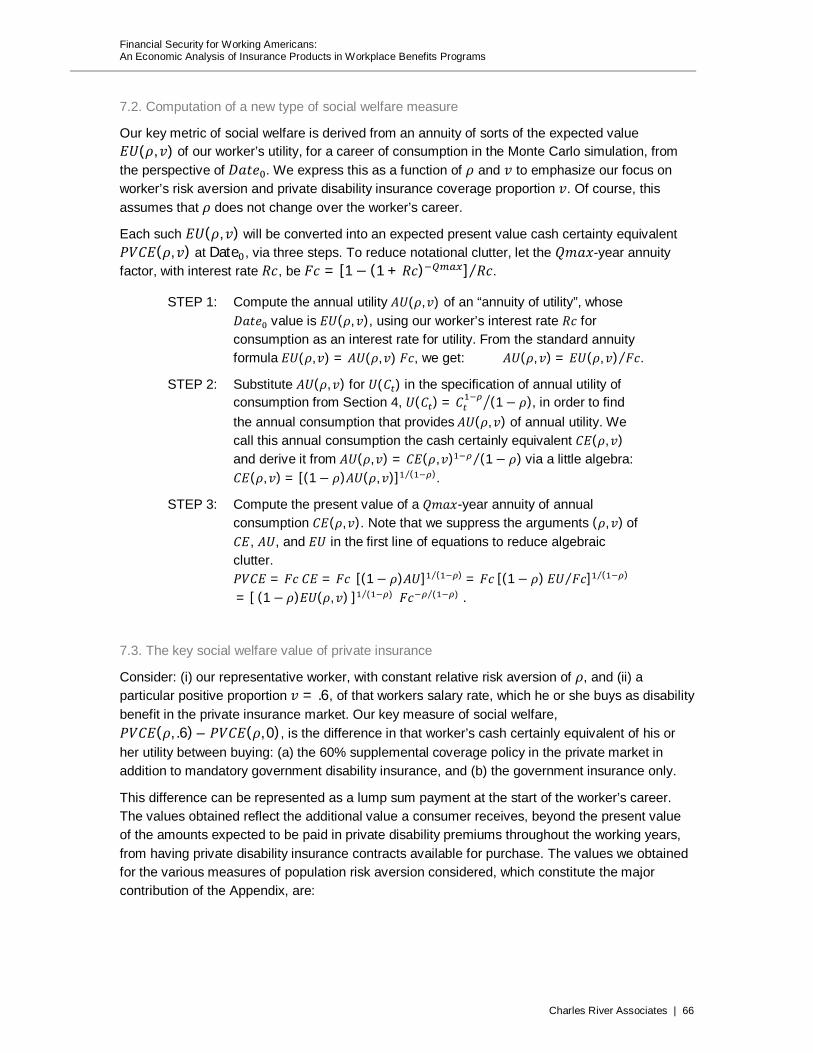
Financial Security for Working Americans: An Economic Analysis of Insurance Products in Workplace Benefits Programs
Charles River Associates | 66
7.2. Computation of a new type of social welfare measure
Our key metric of social welfare is derived from an annuity of sorts of the expected value 퐸푈(휌, 푣) of our worker’s utility, for a career of consumption in the Monte Carlo simulation, from the perspective of 퐷푎푡푒 . We express this as a function of 휌 and 푣 to emphasize our focus on worker’s risk aversion and private disability insurance coverage proportion 푣. Of course, this assumes that 휌 does not change over the worker’s career.
Each such 퐸푈(휌, 푣) will be converted into an expected present value cash certainty equivalent 푃푉퐶퐸(휌, 푣) at Date , via three steps. To reduce notational clutter, let the 푄푚푎푥-year annuity factor, with interest rate 푅푐, be 퐹푐 = [1 − (1 + 푅푐) ] 푅푐⁄ .
STEP 1: Compute the annual utility 퐴푈(휌, 푣) of an “annuity of utility”, whose 퐷푎푡푒 value is 퐸푈(휌, 푣), using our worker’s interest rate 푅푐 for consumption as an interest rate for utility. From the standard annuity formula 퐸푈(휌, 푣) = 퐴푈(휌, 푣) 퐹푐, we get: 퐴푈(휌, 푣) = 퐸푈(휌, 푣) 퐹푐⁄ .
STEP 2: Substitute 퐴푈(휌, 푣) for 푈(퐶 ) in the specification of annual utility of consumption from Section 4, 푈(퐶 ) = 퐶 (1 − 휌), in order to find the annual consumption that provides 퐴푈(휌, 푣) of annual utility. We call this annual consumption the cash certainly equivalent 퐶퐸(휌, 푣) and derive it from 퐴푈(휌, 푣) = 퐶퐸(휌, 푣) (1 − 휌)⁄ via a little algebra: 퐶퐸(휌, 푣) = [(1 − 휌)퐴푈(휌, 푣)] ( )⁄ .
STEP 3: Compute the present value of a 푄푚푎푥-year annuity of annual consumption 퐶퐸(휌, 푣). Note that we suppress the arguments (휌, 푣) of 퐶퐸, 퐴푈, and 퐸푈 in the first line of equations to reduce algebraic clutter. 푃푉퐶퐸 = 퐹푐 퐶퐸 = 퐹푐 [(1 − 휌)퐴푈] ( )⁄ = 퐹푐 [(1 − 휌) 퐸푈 퐹푐⁄ ] ( )⁄ = [ (1 − 휌)퐸푈(휌, 푣) ] (⁄ ) 퐹푐 ( )⁄ .
7.3. The key social welfare value of private insurance
Consider: (i) our representative worker, with constant relative risk aversion of 휌, and (ii) a particular positive proportion 푣 = .6, of that workers salary rate, which he or she buys as disability benefit in the private insurance market. Our key measure of social welfare, 푃푉퐶퐸(휌, .6) – 푃푉퐶퐸(휌, 0), is the difference in that worker’s cash certainly equivalent of his or her utility between buying: (a) the 60% supplemental coverage policy in the private market in addition to mandatory government disability insurance, and (b) the government insurance only.
This difference can be represented as a lump sum payment at the start of the worker’s career. The values obtained reflect the additional value a consumer receives, beyond the present value of the amounts expected to be paid in private disability premiums throughout the working years, from having private disability insurance contracts available for purchase. The values we obtained for the various measures of population risk aversion considered, which constitute the major contribution of the Appendix, are:
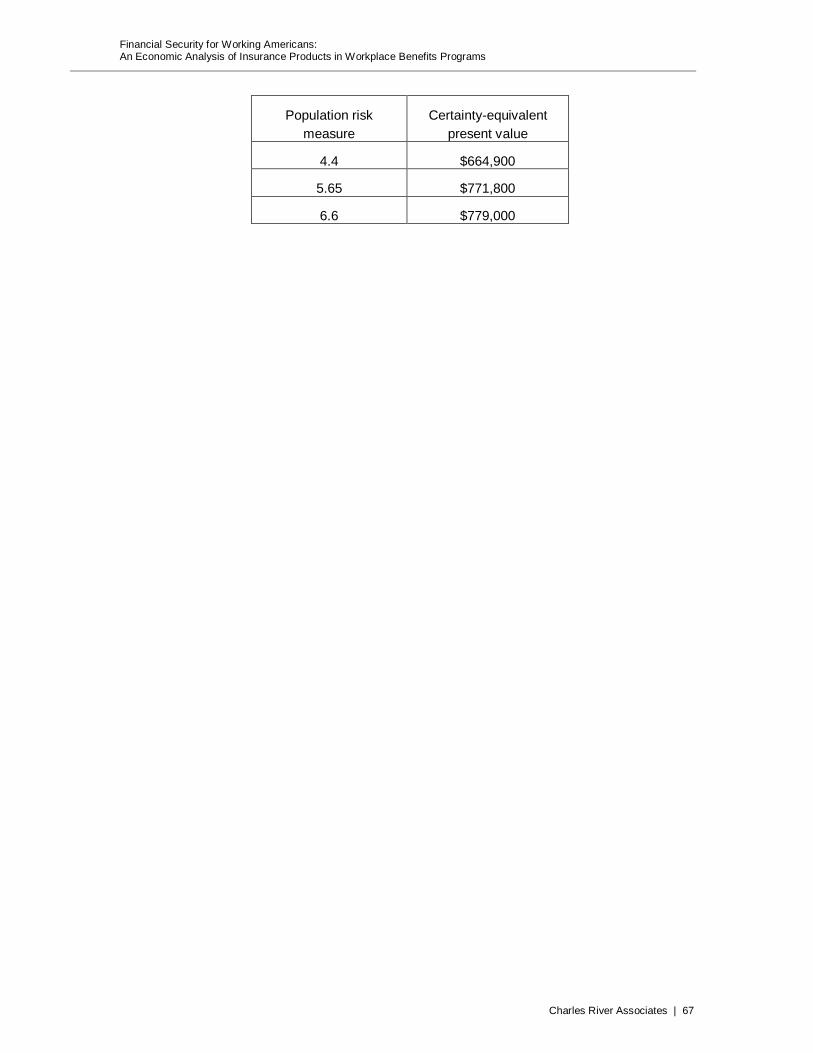
Financial Security for Working Americans: An Economic Analysis of Insurance Products in Workplace Benefits Programs
Charles River Associates | 67
Population risk measure
Certainty-equivalent present value
4.4 $664,900
5.65 $771,800
6.6 $779,000