The Power of Alternative Kolmogorov-Smirnov Tests Based …ww2040/Kim_Whitt_TOMACS_2015.pdf · The Kolmogorov-Smirnov (KS) statistical test is commonly used to determine if data can

24

The Power of Alternative Kolmogorov-Smirnov Tests Basedon Transformations of the Data

SONG-HEE KIM, Yale UniversityWARD WHITT, Columbia University

The Kolmogorov-Smirnov (KS) statistical test is commonly used to determine if data can be regarded as asample from a sequence of independent and identically distributed (i.i.d.) random variables with specifiedcontinuous cumulative distribution function (cdf) F, but with small samples it can have insufficient power,that is, its probability of rejecting natural alternatives can be too low. However, in 1961, Durbin showed thatthe power of the KS test often can be increased, for a given significance level, by a well-chosen transformationof the data. Simulation experiments reported here show that the power can often be more consistently andsubstantially increased by a different transformation. We first transform the given sequence to a sequenceof mean-1 exponential random variables, which is equivalent to a rate-1 Poisson process. We then applythe classical conditional-uniform transformation to convert the arrival times into i.i.d. random variablesuniformly distributed on [0, 1]. And then, after those two preliminary steps, we apply the original Durbintransformation. Since these KS tests assume a fully specified cdf, we also investigate the consequence ofhaving to estimate parameters of the cdf.

Categories and Subject Descriptors: I.6.5 [Simulation and Modeling]: Model Development

General Terms: Theory

Additional Key Words and Phrases: Hypothesis tests, Kolmogorov-Smirnov statistical test, power, datatransformations

ACM Reference Format:Song-Hee Kim and Ward Whitt. 2015. The power of alternative Kolmogorov-Smirnov tests based on trans-formations of the data. ACM Trans. Model. Comput. Simul. 25, 4, Article 24 (May 2015), 22 pages.DOI: http://dx.doi.org/10.1145/2699716

1. INTRODUCTION

We are pleased to contribute to this special issue honoring Donald L. Iglehart, ouracademic grandfather and father, respectively. Don deserves recognition in this journalbecause of the research he and his students have done on simulation methodology, forexample, Crane and Iglehart [1974a, 1974b, 1975], Glynn and Iglehart [1989], andHeidelberger and Iglehart [1979].

We consider the basic statistical problem of testing whether observations can be re-garded as a sample from a sequence of independent and identically distributed (i.i.d.)random variables with a specified cumulative distribution function (cdf). Such testingcommonly should be done in simulation input modeling, for example, to judge whether

This work is supported by the U.S. National Science Foundation grants CMMI 1066372 and 1265070 and bythe Samsung Foundation.Authors’ addresses: S.-H. Kim, Yale School of Management, Yale University, New Haven, CT 06520; email:[email protected]; W. Whitt, Department of Industrial Engineering and Operations Research,Columbia University, New York, NY 10027; email: [email protected] to make digital or hard copies of part or all of this work for personal or classroom use is grantedwithout fee provided that copies are not made or distributed for profit or commercial advantage and thatcopies show this notice on the first page or initial screen of a display along with the full citation. Copyrights forcomponents of this work owned by others than ACM must be honored. Abstracting with credit is permitted.To copy otherwise, to republish, to post on servers, to redistribute to lists, or to use any component of thiswork in other works requires prior specific permission and/or a fee. Permissions may be requested fromPublications Dept., ACM, Inc., 2 Penn Plaza, Suite 701, New York, NY 10121-0701 USA, fax +1 (212)869-0481, or [email protected]© 2015 ACM 1049-3301/2015/05-ART24 $15.00

DOI: http://dx.doi.org/10.1145/2699716

ACM Transactions on Modeling and Computer Simulation, Vol. 25, No. 4, Article 24, Publication date: May 2015.

http://dx.doi.org/10.1145/2699716

http://dx.doi.org/10.1145/2699716

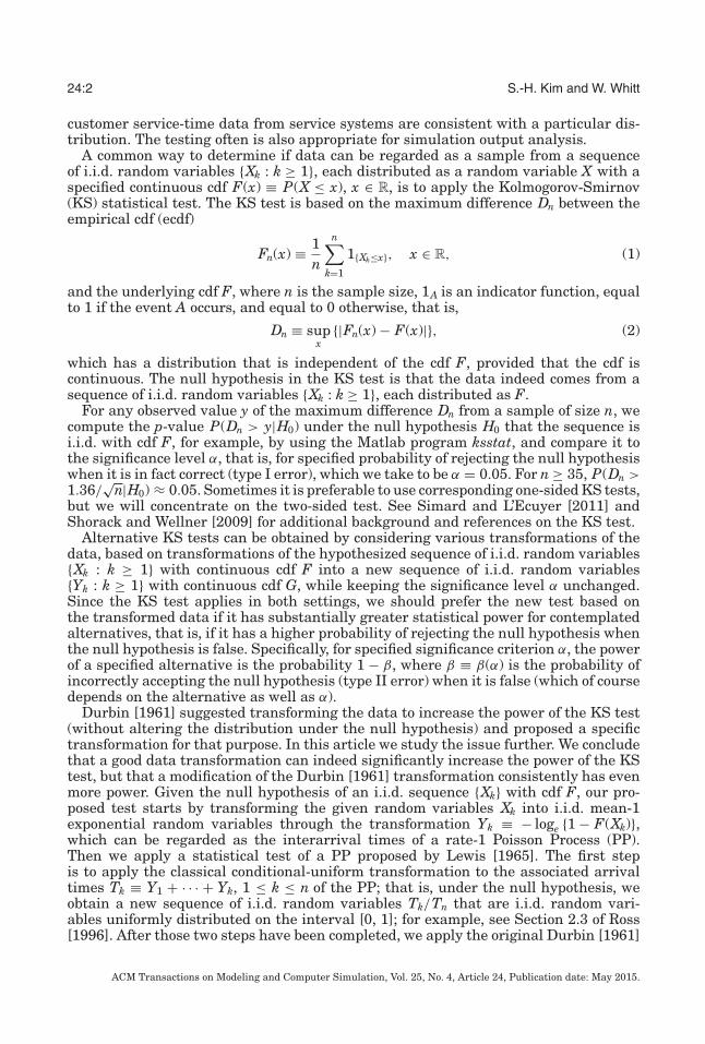
24:2 S.-H. Kim and W. Whitt

customer service-time data from service systems are consistent with a particular dis-tribution. The testing often is also appropriate for simulation output analysis.

A common way to determine if data can be regarded as a sample from a sequenceof i.i.d. random variables {Xk : k ≥ 1}, each distributed as a random variable X with aspecified continuous cdf F(x) ≡ P(X ≤ x), x ∈ R, is to apply the Kolmogorov-Smirnov(KS) statistical test. The KS test is based on the maximum difference Dn between theempirical cdf (ecdf)

Fn(x) ≡ 1n

n∑k=1

1{Xk≤x}, x ∈ R, (1)

and the underlying cdf F, where n is the sample size, 1A is an indicator function, equalto 1 if the event A occurs, and equal to 0 otherwise, that is,

Dn ≡ supx

{|Fn(x) − F(x)|}, (2)

which has a distribution that is independent of the cdf F, provided that the cdf iscontinuous. The null hypothesis in the KS test is that the data indeed comes from asequence of i.i.d. random variables {Xk : k ≥ 1}, each distributed as F.

For any observed value y of the maximum difference Dn from a sample of size n, wecompute the p-value P(Dn > y|H0) under the null hypothesis H0 that the sequence isi.i.d. with cdf F, for example, by using the Matlab program ksstat, and compare it tothe significance level α, that is, for specified probability of rejecting the null hypothesiswhen it is in fact correct (type I error), which we take to be α = 0.05. For n ≥ 35, P(Dn >1.36/

√n|H0) ≈ 0.05. Sometimes it is preferable to use corresponding one-sided KS tests,

but we will concentrate on the two-sided test. See Simard and L’Ecuyer [2011] andShorack and Wellner [2009] for additional background and references on the KS test.

Alternative KS tests can be obtained by considering various transformations of thedata, based on transformations of the hypothesized sequence of i.i.d. random variables{Xk : k ≥ 1} with continuous cdf F into a new sequence of i.i.d. random variables{Yk : k ≥ 1} with continuous cdf G, while keeping the significance level α unchanged.Since the KS test applies in both settings, we should prefer the new test based onthe transformed data if it has substantially greater statistical power for contemplatedalternatives, that is, if it has a higher probability of rejecting the null hypothesis whenthe null hypothesis is false. Specifically, for specified significance criterion α, the powerof a specified alternative is the probability 1 − β, where β ≡ β(α) is the probability ofincorrectly accepting the null hypothesis (type II error) when it is false (which of coursedepends on the alternative as well as α).

Durbin [1961] suggested transforming the data to increase the power of the KS test(without altering the distribution under the null hypothesis) and proposed a specifictransformation for that purpose. In this article we study the issue further. We concludethat a good data transformation can indeed significantly increase the power of the KStest, but that a modification of the Durbin [1961] transformation consistently has evenmore power. Given the null hypothesis of an i.i.d. sequence {Xk} with cdf F, our pro-posed test starts by transforming the given random variables Xk into i.i.d. mean-1exponential random variables through the transformation Yk ≡ − loge {1 − F(Xk)},which can be regarded as the interarrival times of a rate-1 Poisson Process (PP).Then we apply a statistical test of a PP proposed by Lewis [1965]. The first stepis to apply the classical conditional-uniform transformation to the associated arrivaltimes Tk ≡ Y1 + · · · + Yk, 1 ≤ k ≤ n of the PP; that is, under the null hypothesis, weobtain a new sequence of i.i.d. random variables Tk/Tn that are i.i.d. random vari-ables uniformly distributed on the interval [0, 1]; for example, see Section 2.3 of Ross[1996]. After those two steps have been completed, we apply the original Durbin [1961]


The Power of Alternative Kolmogorov-Smirnov Tests Based on Transformations of the Data 24:3

transformation. While the component transformations that we use are not new, to thebest of our knowledge, this combination of transformations has not been considered be-fore. The idea of considering this alternative KS test came to us while working on waysto test if service-system arrival process data can be modeled as a nonhomogeneous PP,which is reported in Kim and Whitt [2014a, 2014b] and Kim et al. [2015]; we elaborateafter we define the alternative tests that we examine.

We close this introduction by indicating how the rest of the article is organized. Westart in Section 2 by carefully defining the six different KS tests we consider. Next,in Section 3, we elaborate on our motivation and explain why the new method shouldbe promising. In Section 4 we describe our first simulation experiment, which is afixed-sample-size discrete-time stationary-sequence analog of the fixed-interval-lengthcontinuous-time stationary point process experiment, aimed at studying tests of a PP,conducted in Kim and Whitt [2014b]. In addition to the natural null hypothesis ofi.i.d. exponential random variables, we also consider i.i.d. nonexponential sequenceswith Erlang, hyperexponential, and lognormal marginal cdf ’s. We report the results inSection 5, which surprisingly show that the original Durbin [1961] method performspoorly, but we consider different models than those in Durbin [1961]. In contrast, ournew method, which we call the Lewis test because it is based on an idea from Lewis[1965], performs well, providing increased power. However, Durbin [1961] considereddifferent examples. Motivated by the good results found for a standard normal nullhypothesis by Durbin [1961], in Section 6 we consider a second experiment to testfor a sequence of i.i.d. standard normal random variables. Consistent with Durbin[1961], we find that the original Durbin [1961] method performs much better for thestandard normal null hypothesis, but again the new version of the Lewis [1965] testalso performs well. In Section 7 we discuss the common problem that we typically mustestimate parameters when we apply the KS test. We draw conclusions in Section 8.Additional information appears in the online Appendix.

2. THE ALTERNATIVE KS TESTS

We consider the following six KS tests of the null hypothesis H0 that n observationsXk, 1 ≤ k ≤ n, can be considered a sample from a sequence of i.i.d. random variableshaving a continuous cdf F. We start by forming the associated variables Uk ≡ F(Xk),which are i.i.d. uniform variables on [0, 1] under the null hypothesis.

Standard Test. We use the standard KS test based on (2) to test whether Uk ≡ F(Xk),1 ≤ k ≤ n, can be considered to be i.i.d. random variables uniformly distributedon [0, 1].

Sort-Log Test. Starting with the n random variables Uk, 1 ≤ k ≤ n, in the standardtest, let U( j) be the jth smallest of these, so that U(1) < · · · < U(n). As in Section 3.1of Brown et al. [2005], we use the fact that under the null hypothesis

Y (L)j ≡ − j loge

(U( j)/U( j+1)

), 1 ≤ j ≤ n − 1,

are n−1 i.i.d. mean-1 exponential random variables; a proof is given in Section 2.2of Kim and Whitt [2014c]. We then apply the KS test with n replaced by n− 1 andthe mean-1 exponential cdf.

Durbin (≡ Sort-Durbin) Test. This is the original test proposed by Durbin [1961],which also starts with Uk ≡ F(Xk) and U(k) with U(1) < · · · < U(n) as previously. Inthis context, look at the successive intervals between these ordered observations:

C1 ≡ U(1), Cj ≡ U( j) − U( j−1), 2 ≤ j ≤ n + 1, and Cn+1 ≡ 1 − U(n).

Then let C( j) be the jth smallest of these intervals, 1 ≤ j ≤ n, so that 0 < C(1) <· · · < C(n+1) < 1. Now let Zj be scaled versions of the intervals between these new



ordered intervals, that is, let

Zj = (n + 2 − j)(C( j) − C( j−1)), 1 ≤ j ≤ n + 1, (with C(0) ≡ 0). (3)

Remarkably, Durbin [1961] showed (by a simple direct argument giving explicitexpressions for the joint density functions, exploiting the transformation of ran-dom vectors by a function) that, under the null hypothesis, the random vector(Z1, . . . , Zn) is distributed the same as the random vector (C1, . . . , Cn). Hence,again under the null hypothesis, the vector of associated partial sums (S1, . . . , Sn),where Sk ≡ Z1 + · · · + Zk, 1 ≤ k ≤ n, has the same distribution as the originalrandom vector (U(1), . . . ,U(n)) of ordered uniform random variables. Hence, we canapply the KS test with the ecdf

Fn(x) ≡ n−1n∑

k=1

1{Sk≤x}, 0 ≤ x ≤ 1,

for Sk above, comparing it to the uniform cdf on [0, 1].

CU (Conditional-Uniform ≡ Exp+CU) Test. We start with Yk ≡ − loge {1 − F(Xk)},1 ≤ k ≤ n, which are i.i.d. mean-1 exponential random variables under the nullhypothesis. Thus, the cumulative sums Tk ≡ Y1 + · · · + Yk, 1 ≤ k ≤ n, are thearrival times of a rate-1 PP. In this context, the conditional-uniform propertystates that, under the null hypothesis, Tk/Tn, 1 ≤ k ≤ n − 1, are distributed asthe order statistics of n− 1 i.i.d. random variables uniformly distributed on [0, 1].Thus we can apply the KS statistic with the ecdf

F (CU )n (x) ≡ 1

n − 1

n−1∑k=1

1{(Tk/Tn)≤x}, 0 ≤ x ≤ 1, (4)

and the underlying uniform cdf on [0, 1].

Log (Exp+CU+Log) Test. We start with the partial sums Tk, 1 ≤ k ≤ n, used in theCU test, which are the arrival times of a rate-1 PP under the null hypothesis. Weagain use the conditional-uniform property for fixed sample size to conclude that,under the null hypothesis, Tk/Tn, 1 ≤ k ≤ n− 1, are distributed as U(k), the orderstatistics of n− 1 random variables, with U(1) < · · · < U(n−1). Hence, just as in theprevious Sort-Log test,

Y (L)j ≡ − j loge

(Tj/Tj+1

), 1 ≤ j ≤ n − 1,

should be n − 1 i.i.d. rate-1 exponential random variables, to which we can applythe KS test.

Lewis (Exp+CU+Durbin) Test. We again start with the partial sums Tk, 1 ≤ k ≤ n,used in the CU test, which are the arrivals times of a rate-1 PP under the nullhypothesis. We again use the conditional-uniform property for fixed sample sizeto conclude that, under the null hypothesis, Tk/Tn, 1 ≤ k ≤ n − 1, are distributedas U(k), the order statistics of n− 1 random variables uniformly distributed on [0,1], with U(1) < · · · < U(n−1). From this point, we apply the previously mentionedDurbin [1961] test with n replaced by n− 1, just as Lewis [1965] did in his test ofa PP.

3. MOTIVATION AND EXPLANATION

In this section, we describe our motivation for considering these new KS tests and weexplain why the good performance we find in our experiments might be anticipated.



3.1. Testing if Arrival Processes Can be Regarded as Nonhomogeneous Poisson Processes

Our research was motivated by the desire to fit stochastic queueing models to datafrom large-scale service systems, such as telephone call centers and hospital emergencyrooms, as discussed in Brown et al. [2005] and Armony et al. [2011]. These queueingmodels typically possess at least two stochastic elements that might be tested: arrivalprocesses and service times. We started by looking at the arrival processes.

Since the arrival rate typically varies strongly by time of day in these service sys-tems, the natural arrival process model is a nonhomogeneous PP (NHPP). The Poissonproperty arises from many people acting independently, each of whom uses the servicesystem infrequently. Mathematical support is provided by the Poisson superpositiontheorem (see Section 9.8 of Whitt [2002], and references therein).

However, as emphasized by Brown et al. [2005], it is important to perform statisticaltests on arrival data to see if the NHPP model is appropriate. For that purpose, Brownet al. [2005] proposed a variant of the Log KS test. First, Brown et al. [2005] assumedthat the arrival rate function can be approximated by a Piecewise-Constant (PC) arrivalrate function, which is often reasonable, because the arrival rate evidently changesrelatively slowly. (We investigate how the subintervals should be chosen in Kim andWhitt [2014a].) Under the PC NHPP null hypothesis, the NHPP is then equivalent to aPP over each subinterval where the rate is constant. Then Brown et al. [2005] appliedthe CU transformation over each of these subintervals. Since the CU transformationis independent of the rate of the PP, the CU transformation can be applied to eachinterval where the rate is constant, and then all the data can be combined into a singlesequence of i.i.d. random variables uniformly distributed on [0, 1].

For a PC NHPP, we strongly exploit the fact that the CU transformation eliminates allnuisance parameters. We need not estimate the rate on each of the many subintervals.As a consequence, however, the KS test after applying the CU transformation does notsupport any given arrival rate, and even allows it to be random. Thus, as discussed inKim and Whitt [2014a, 2014b], the KS test might also be regarded as being for a Coxprocess, that is, a PP with a rate function that is a stochastic process. However, thepossible rate stochastic processes are greatly restricted by the requirement that therate be constant over each subinterval over which the CU property is applied.

After applying the CU transformation in that way to the PC NHPP, it is possible toapply the standard KS test directly, but Brown et al. [2005] did not do that. Instead,they performed the Log test. They then justified an NHPP model for the banking callcenter arrival data they were studying by showing that they could not reject the PPhypothesis with their Log KS test.

We wondered why Brown et al. [2005] applied the Log test with the additional loga-rithmic transformation instead of applying the CU KS test. As we presumed must bethe case, we found that the CU KS test of a PP has remarkably little power againstcommon alternative hypotheses such as renewal processes with nonexponential inter-arrival time distributions. We present theoretical support via asymptotic analysis andempirical evidence from extensive simulation experiments in Kim and Whitt [2014b].

We also found that there is a substantial history in the statistical literature. First,Lewis [1965] made a significant contribution for testing a PP, recognizing that theDurbin [1961] transformation could be effectively applied after the CU transformation.Second, from Lewis [1965] we discovered that the direct CU KS test of a PP wasevidently first proposed by Barnard [1953]; and Lewis [1965] showed that it had littlepower.

Upon discovering Lewis [1965], we first supposed that the Log KS test of Brown et al.[2005] would turn out to be equivalent to the Lewis [1965] transformation and that theKS test proposed by Lewis [1965], drawing upon Durbin [1961], would coincide with theKS test given in Durbin [1961], but neither is the case. Thus, this past work suggests



several different KS tests. In Kim and Whitt [2014b], we concluded that the Lewis testof a PP has the most power against stationary point processes having nonexponentialinterarrival distributions, providing a significant improvement over the Log KS test.

On the other hand, we also found that none of the KS tests has much power againststationary point processes with dependent exponential interarrival times, that is, whichdiffer from a PP only through the dependence. In fact, for those alternative hypotheses,we found the CU KS test tended to be most effective.

3.2. The Explanation

The key insight is the observation that the uniform random variables in the CU KStest are very different from the uniform random variables in the Standard KS test.Under the null hypothesis of i.i.d. exponential variables, these exponential variablesdirectly correspond to the interarrival times of a PP. The uniform random variables inthe standard test are direct transformations of these interarrival times, one by one.

In contrast, the uniform random variables produced by the CU transformation ap-plied to the PP correspond to the successive arrival times in the PP, that is, the cu-mulative sums of the interarrival times. As a consequence, the CU KS test is evidentlyless able to detect differences in the interarrival-time distribution. In Section 7 ofKim and Whitt [2014b] we provide mathematical support by proving that the ecdf inEquation (1) converges to the uniform cdf as the sample size n increases for any rate-1stationary ergodic point process, that is, for any stationary point process satisfying astrong law of large numbers. Thus, to first order, asymptotically, the CU KS test hasno power at all against any of the alternatives in this large class.

This insight also helps explain why the Lewis test does so much better. It appliesthe Durbin transformation after performing the CU transformation. However, the firststep of the Durbin transformation is to focus on the interarrival times and put themin ascending order. Thus, the Durbin transformation strongly brings the focus back tothe interarrival times.

This advantage of the Lewis test is well illustrated by the problem of data rounding,which is studied in Kim and Whitt [2014a]. In applications, the data are often rounded,for example, to the nearest second. With large datasets, this produces zero-lengthinterarrival times. Before applying the Durbin transformation, these are spread outthroughout the data, so that they tend not to be detected by the KS test. On the otherhand, the Durbin transformation shifts all these zero-length interarrival times to theleft end of the distribution, leading to rejection. This is easy to see in the plots of theecdfs.

The reordering property of the Durbin transformation also helps explain why theCU KS test tends to do relatively well against dependent exponential sequences. Thereordering of the interarrival times, which is helpful for identifying nonexponentialdistributions, tends to dissipate the dependence among dependent exponential randomvariables. The cumulative impact of the dependence evidently can best be seen throughthe cumulative sums of the interarrival times, that is, the arrival times, without re-ordering.

4. THE FIRST EXPONENTIAL EXPERIMENT

Our first simulation experiment is for the discrete-time analog of the experiment fortesting the continuous-time PP in Kim and Whitt [2014b]. To study the alternative KStests of a PP, in Kim and Whitt [2014b] we let the null hypothesis in the base case bea rate-1 PP observed over the time interval [0, 200], so that the expected sample sizewas 200, but we also considered the longer time interval [0, 2,000].

Hence, closely paralleling that experimental design, our null hypothesis here in thebase case is a sample of size n = 200 i.i.d. mean-1 exponential random variables, but



to see the impact of the sample size, we also give results for the larger sample size ofn = 2,000.

Closely linking the experiments helps make insightful comparisons. From an applica-tions perspective, the exponential distribution is also a natural reference case, becausethe exponential distribution is often assumed for service times as well as interarrivaltimes in queueing models in order that associated stochastic processes, such as thenumber of customers in the system, will be Markov processes. We are thus developingstatistical tests of Markov model components.

4.1. The Cases Considered

We use the same alternative hypotheses to the continuous-time PP used in Kim andWhitt [2014b], except that we replace the time intervals of fixed length t by samplesizes of fixed size n. That is, we now consider stationary sequences of mean-1 randomvariables. There are nine cases, each with from one to five subcases, yielding 29 casesin all. Again, using the same cases as before facilitates comparison.

The first five cases involve i.i.d. mean-1 random variables; the last four cases involvedependent identically distributed mean-1 random variables. The first i.i.d. case is ournull hypothesis with exponential random variables. The other i.i.d. cases have nonexpo-nential random variables. Cases 2 and 3 contain Erlang and hyperexponential randomvariables, which are, respectively, stochastically less variable and stochastically morevariable than the exponential distribution in convex stochastic order, as in Section 9.5of Ross [1996]. Thus, they have squared coefficient of variation (scv; variance dividedby the square of the mean, denoted by c2), c2 < 1 and c2 > 1, respectively. Thesedistributions show deviations from the exponential distribution in their variability.They are special phase-type distributions, which are also often assumed in order toobtain Markov process models (that are more complicated than when the distributionis exponential); for example, see Neuts [1981].

Cases 4 and 5 contain other i.i.d. sequences with nonexponential cdfs. Case 4 containsa nonexponential distribution with the same scv c2 = 1 as the exponential distribution,as well as E[X] = 1, while Case 5 contains lognormal distributions, with four differentscvs. Lognormal distributions often have been found to fit service-time data well (e.g.,see Brown et al. [2005]).

Case 1, Exponential. The null hypothesis with i.i.d. mean-1 exponential randomvariables (Base Case).

Case 2, Erlang, Ek. Erlang-k (Ek) random variables, a sum of k i.i.d. exponentialsfor k = 2, 4, 6 with c2

X ≡ c2k = 1/k .

Case 3, Hyperexponential, H2. Hyperexponential-2 (H2) random variables, a mix-ture of two exponential cdfs with c2

X = 1.25, 1.5, 2, 4, and 10 (five cases).The cdf is P(X ≤ x) ≡ 1 − p1e−λ1x − p2e−λ2x. We further assume balancedmeans (p1λ

−11 = p2λ

−12 ) as in (3.7) of Whitt [1982] so that given the value of

c2X, pi = [1 ±

√(c2

X − 1)/(c2X + 1)]/2 and λi = 2pi.

Case 4, mixture with c2X = 1. A mixture of a more variable cdf and a less variable

cdf so that the c2X = 1; P(X = Y ) = p = 1 − P(X = Z), where Y is H2 with c2

Y = 4,Z is E2 with c2

Z = 1/2, and p = 1/7.

Case 5, lognormal, LN. Lognormal (LN(1, σ 2)) random variables with mean 1 andvariance σ 2 for σ 2 = c2

X = 0.25, 1.0, 4.0, 10.0 (four cases).



Cases 6 and 7 are dependent stationary sequences that deviate from the null hypoth-esis (Case 1) only through dependence among successive variables, each exponentiallydistributed with mean 1. It is not customary to test for dependence among successiveservice times in applications, but see Gans et al. [2010]. We think that it deserves moreattention. Toward that end, we consider the two cases:

Case 6, RRI, dependent exponential interarrival times. Randomly Repeated Interar-rival (RRI) times with exponential interarrival times, constructed by letting eachsuccessive interarrival time be a mixture of the previous interarrival time withprobability p or a new independent interarrival time from an exponential distri-bution with mean 1, with probability 1 − p (a special case of a first-order DiscreteAutoregressive process, DAR(1), studied by Jacobs and Lewis [1978, 1983]). Itsserial correlation is Corr(Xj, Xj+k) = pk. We consider three values of p: 0.1, 0.5,and 0.9.

Case 7, EARMA, dependent exponential interarrival times. A stationary sequenceof dependent exponential interarrival times with the correlation structure of anautoregressive-moving average process, called EARMA(1,1) in Jacobs and Lewis[1977]. Starting from three independent sequences of i.i.d. random variables {Xn :n ≥ 0}, {Un : n ≥ 1}, and {Vn : n ≥ 1}, where Y0 and Xn, n ≥ 1, are exponentiallydistributed with mean m = 1, while

P(Un = 0) = 1 − P(Un = 1) = β and P(Vn = 0) = 1 − P(Vn = 1) = ρ, (5)

the EARMA sequence {Sn : n ≥ 1} is defined recursively by

Sn = βXn + UnYn−1,

Yn = ρYn−1 + VnXn, n ≥ 1. (6)

Its serial correlation is Corr(Sj, Sj+k) = γρk−1, where γ = β(1−β)(1−ρ)+(1−β)2ρ.We consider five cases of (β, ρ): (0.75, 0.50), (0.5, 0.5), (0.5, 0.75), (0.00, 0.75), and(0.25, 0.90) so that the cumulative correlations

∑∞k=1 Corr(Sj, Sj+k) increase: 0.25,

0.50, 1.00, 3.00, and 5.25. For more details, see Pang and Whitt [2012]. We specifythese cases by these cumulative correlations.

The final two cases are stationary sequences that have both nonexponential marginaldistributions and dependence among successive variables:

Case 8, mH2, superposition of m i.i.d. H2 renewal processes. A stationary sequence ofinterarrival times from a superposition of m i.i.d. equilibrium renewal processes,where the times between renewals (interarrival times) in each renewal processhas a hyperexponential (H2) distribution with c2

a = 4 (mH2). As the number mof component renewal processes increases, the superposition process convergesto a PP, and thus looks locally more like a PP, with the interarrival distributionapproaching exponential and the lag-k correlations approaching 0, but small cor-relations extending further across time, so that the superposition process retainsan asymptotic variability parameter, c2

A = 4. We consider four values of m: 2, 5,10, and 20.

Case 9, RRI (H2), dependent H2 interarrival times with c2 = 4. RRI times with H2interarrival times, each having mean 1, c2 = 4 and balanced means (as specifiedin Case 3). The repetition is done just as in Case 6. We again consider three valuesof p: 0.1, 0.5, and 0.9.

Cases 6 and 7 have short-range dependence, whereas Case 8 for large m tends tohave nearly exponential interarrival times, but longer-range dependence. For small



m, the mH2 superposition process should behave much like the H2 renewal process inCase 3 with the component c2 = 4; for large m, the mH2 superposition process shouldbehave more like Cases 6 and 7 with dependence and exponential interarrival times.

Since the new KS tests apply to i.i.d. sequences with arbitrary continuous cdfs, wealso consider alternative null hypotheses. In particular, here we report results for E2,H2 (with c2 = 2), and lognormal LN(1, 4) (with c2 = 4) marginal cdfs having mean 1 aswell as the exponential base case.

4.2. Simulation Design

For each case, we simulated 104 replications of 3,000 interarrival times. We generatemuch more data than needed in order to get rid of any initial effects. We are supposingthat we observe a stationary sequence. There is, of course, no problem if the sequenceis i.i.d. However, for the dependent sequences, stationarity is achieved approximatelyby having the system operate for some time before collecting data. The initial effectwas observed to matter for the cases with dependent interarrival times and relativelysmall sample sizes.

We use this simulation output to generate sample sizes of a fixed size n. With fixedsample size n = 200, in each replication of the 104 simulated interarrival times we useinterarrival times from the 103th interarrival time to the 103 +200th interarrival time.To consider large sample sizes, we increased n from 200 to 2,000. We then consider theinterarrival times from the 103th interarrival time to the 103 + 2,000th interarrivaltime to observe the effect of larger sample size. This choice leaves little doubt aboutthe stationarity assumption.

For each sample, we checked our simulation results by estimating the mean and scvof each interarrival-time cdf both before and after transformations; tables of the resultsand plots of the average of the ecdfs appear in the online Appendix.

5. RESULTS OF THE FIRST EXPERIMENT

The online Appendix contains detailed results of the experiments; we present a sum-mary here. First, we found that the sort-Log and Log tests were consistently dominatedby the Durbin [1961] test or the Lewis [1965] test, so we do not present detailed resultsfor those two Log cases here. For the CU, CU+Log, and Lewis tests, we consideredvariants based on the exponential variables − loge {F(X)} and well as − loge {1 − F(X)},but we did not find great differences, so we do not report those either. Thus, we presentthe results of four KS tests: (i) the standard test, using the variables Uk ≡ F(Xk),(ii) the Durbin [1961] test, (iii) the CU test, and (iv) the Lewis [1965] test, as specifiedin Section 2. Under the null hypotheses, the cdf in all four cases is uniform on [0, 1].

5.1. The Base Case: i.i.d. Mean-1 Exponential Variables

For our base case, we let the null hypothesis H0 be that the data are from i.i.d. mean-1 exponential variables. We report the number of KS tests passed (not rejected) outof 10,000 replications as well as the average p-value with associated 95% confidenceintervals. Thus, the estimate of the power is 1−(number passed/10,000). The p-value isthe significance level below which the hypothesis would be rejected. Thus low p-valuesindicate greater power. Just as in Table 1 of Kim and Whitt [2014b], the differences inthe tests is striking for the middle H2 alternative with c2 = 2.0, as shown in Table Ihere. The results for the Lewis, standard, and CU tests are very similar to those forthe corresponding KS tests of a PP in Table 1 of Kim and Whitt [2014b], but the resultsfor the Durbin [1961] test are new, and surprisingly bad.

The results for all 29 cases are given in Table II. The first “exponential” case is thei.i.d. exponential null hypothesis. The results show that all tests behave properly forthe i.i.d. exponential null hypothesis. The results also show that the tests perform quite



Table I. The Power of Alternative KS Tests of the Null Hypothesisthat Data are i.i.d. Mean-1 Exponential Variables for the SampleSize n = 200 with Significance Level α = 0.05: The Alternative

Hypothesis of i.i.d. H2 Interarrival Times having c2X = 2

KS test Lewis Standard CU DurbinPower 0.93 0.64 0.28 0.14Average p-value 0.02 0.09 0.24 0.40

Table II. The Power of Alternative KS Tests of the Null Hypothesis that Data are i.i.d. Mean-1 ExponentialVariables for the Sample Size n = 200 for Various Alternative Hypotheses: Number of KS Tests Passed (denotedby #P) at Significance Level 0.05 out of 10,000 Replications and the Average p-Values (denoted by E [ p-value ])

with Associated 95% Confidence Intervals

Standard Durbin CU LewisCase Subcase #P E[p-value] #P E[p-value] #P E[p-value] #P E[p-value]

Exp − 9487 0.50 ± 0.0057 9515 0.50 ± 0.0056 9511 0.50 ± 0.0056 9493 0.50 ± 0.0057Ek k = 2 28 0.00 ± 0.0001 3320 0.08 ± 0.0029 9985 0.78 ± 0.0045 0 0.00 ± 0.0000

k = 4 0 0.00 ± 0.0000 0 0.00 ± 0.0000 10,000 0.94 ± 0.0021 0 0.00 ± 0.0000k = 6 0 0.00 ± 0.0000 0 0.00 ± 0.0000 10,000 0.98 ± 0.0011 0 0.00 ± 0.0000

H2 c2 = 1.25 8843 0.42 ± 0.0058 9451 0.49 ± 0.0057 8956 0.41 ± 0.0056 7501 0.30 ± 0.0056c2 = 1.5 7204 0.27 ± 0.0053 9331 0.48 ± 0.0058 8418 0.33 ± 0.0053 3966 0.12 ± 0.0039c2 = 2 3603 0.09 ± 0.0032 8667 0.40 ± 0.0058 7186 0.24 ± 0.0046 695 0.02 ± 0.0013c2 = 4 90 0.00 ± 0.0003 4569 0.13 ± 0.0039 3648 0.08 ± 0.0027 22 0.00 ± 0.0003c2 = 10 0 0.00 ± 0.0000 878 0.02 ± 0.0012 928 0.02 ± 0.0014 67 0.00 ± 0.0006

Mixture − 1200 0.02 ± 0.0009 7016 0.26 ± 0.0053 9438 0.57 ± 0.0061 187 0.00 ± 0.0004LN (1, 0.25) 0 0.00 ± 0.0000 0 0.00 ± 0.0000 10,000 0.94 ± 0.0022 0 0.00 ± 0.0000

(1, 1) 98 0.00 ± 0.0002 3482 0.08 ± 0.0025 9517 0.53 ± 0.0058 24 0.00 ± 0.0001(1, 4) 176 0.00 ± 0.0005 5542 0.18 ± 0.0047 4742 0.13 ± 0.0036 28 0.00 ± 0.0002(1, 10) 0 0.00 ± 0.0000 353 0.01 ± 0.0008 2024 0.04 ± 0.0019 0 0.00 ± 0.0000

RRI p = 0.1 9048 0.41 ± 0.0055 1911 0.03 ± 0.0012 9044 0.42 ± 0.0056 9121 0.41 ± 0.0054p = 0.5 4659 0.11 ± 0.0030 0 0.00 ± 0.0000 5587 0.16 ± 0.0039 4624 0.11 ± 0.0030p = 0.9 16 0.00 ± 0.0001 0 0.00 ± 0.0000 701 0.01 ± 0.0011 13 0.00 ± 0.0001

EARMA 0.25 9284 0.47 ± 0.0058 9475 0.50 ± 0.0057 8564 0.36 ± 0.0055 9498 0.50 ± 0.00570.5 8865 0.43 ± 0.0059 9516 0.50 ± 0.0057 7519 0.27 ± 0.0050 9393 0.49 ± 0.00581 8178 0.37 ± 0.0059 9419 0.50 ± 0.0057 6009 0.19 ± 0.0043 8964 0.44 ± 0.00593 5209 0.21 ± 0.0055 6356 0.23 ± 0.0050 1896 0.04 ± 0.0018 6796 0.30 ± 0.00615.25 4100 0.14 ± 0.0044 8215 0.38 ± 0.0061 1598 0.03 ± 0.0018 5680 0.21 ± 0.0051

mH2 m = 2 4398 0.14 ± 0.0044 8871 0.42 ± 0.0058 4355 0.11 ± 0.0032 1546 0.04 ± 0.0024m = 5 7514 0.32 ± 0.0058 9363 0.48 ± 0.0057 5400 0.17 ± 0.0043 7228 0.29 ± 0.0057m = 10 7818 0.35 ± 0.0060 9423 0.49 ± 0.0057 6562 0.24 ± 0.0051 9004 0.44 ± 0.0059m = 20 7996 0.37 ± 0.0060 9457 0.50 ± 0.0057 7804 0.33 ± 0.0057 9431 0.49 ± 0.0057

RRI(H2) p = 0.1 104 0.00 ± 0.0003 126 0.00 ± 0.0003 2987 0.07 ± 0.0024 37 0.00 ± 0.0003p = 0.5 253 0.00 ± 0.0005 0 0.00 ± 0.0000 1105 0.02 ± 0.0013 215 0.00 ± 0.0006p = 0.9 4 0.00 ± 0.0000 0 0.00 ± 0.0000 229 0.00 ± 0.0005 5 0.00 ± 0.0000

differently for the alternative hypotheses. Table II shows that the standard and Lewistests all perform reasonably well for the i.i.d. cases with nonexponential interarrival-time cdfs, in marked contrast to the CU and Durbin tests. Table II also shows that theLewis test is consistently most powerful for these cases. The ordering remains for H2cdfs with both lower and higher scvs.

Just as in Kim and Whitt [2014b], the story is more complicated for the depen-dent sequences. The Durbin KS test performs remarkably well for the RRI cases, farbetter than all others. Upon further reflection, this makes sense, because the RRIsequence produces strings of identical observations. When the random variables are



Fig. 1. Comparison of the average ecdf based on H2 (c2 = 2) data for 104 replications and n = 200 with thecdf of the exponential null hypothesis: Standard, Durbin, CU, and Lewis tests (from left to right).

Fig. 2. Comparison of the average ecdf based on E2 data for 104 replications and n = 200 with the cdf of theexponential null hypothesis: Standard, Durbin, CU, and Lewis tests (from left to right).

Fig. 3. Comparison of the average ecdf based on LN(1, 4) data for 104 replications and n = 200 with the cdfof the exponential null hypothesis: Standard, Durbin, CU, and Lewis tests (from left to right).

ordered in ascending order, all repeated values will remain next to each other. And then,afterwards, when the Durbin transformation looks at the intervals between the orderedvariables, these intervals will all be 0’s. Hence, all the repetitions will be converted to0’s by the Durbin transformation. That in turn increases F̄n(0) for the ecdf F̄n in Equa-tion (1), which typically increases the KS statistic Dn in Equation (2). It is evident thatthis property is not achieved by any of the other KS tests.

For the RRI(H2) cases, all tests except CU perform very well. Hence, the Lewis test isconsistently superior against nonexponential marginals. As in Kim and Whitt [2014b],none of the tests has much power against the EARMA alternatives, but the CU testhas the most power.

5.2. Plots of the Average Empirical Distributions

As in Kim and Whitt [2014b], we find that useful insight is provided by plots comparingthe average of the ecdfs over all 10,000 replications to the cdf associated with the nullhypothesis, which is uniform in each case here. Figures 1–4 illustrate for the i.i.d.variables having cdfs H2 with c2 = 2, E2, and LN(1, 4), and for the dependent RRI(0.5)variables with n = 200. These figures show that the transformation in the Lewis KStest provides greater separation between the average ecdf and the cdf in the i.i.d. cases.



Fig. 4. Comparison of the average ecdf based on RRI(0.5) data for 104 replications and n = 200 with the cdfof the exponential null hypothesis: Standard, Durbin, CU, and Lewis tests (from left to right).

In each case, the Durbin and Lewis tests tend to produce stochastic order comparedto the uniform cdf, whereas the ecdf crosses over for the standard KS test, which isespecially evident for E2.

We have already observed that the Durbin test excels for RRI because it convertsthe repetitions into 0’s. For RRI with p = 0.5, half of the variables are repetitions.Hence, half of the variables will be transformed into 0’s. That is confirmed by the ecdfassociated with the Durbin test in Figure 4.

5.3. Erlang, Hyperexponential, and Lognormal Null Hypotheses

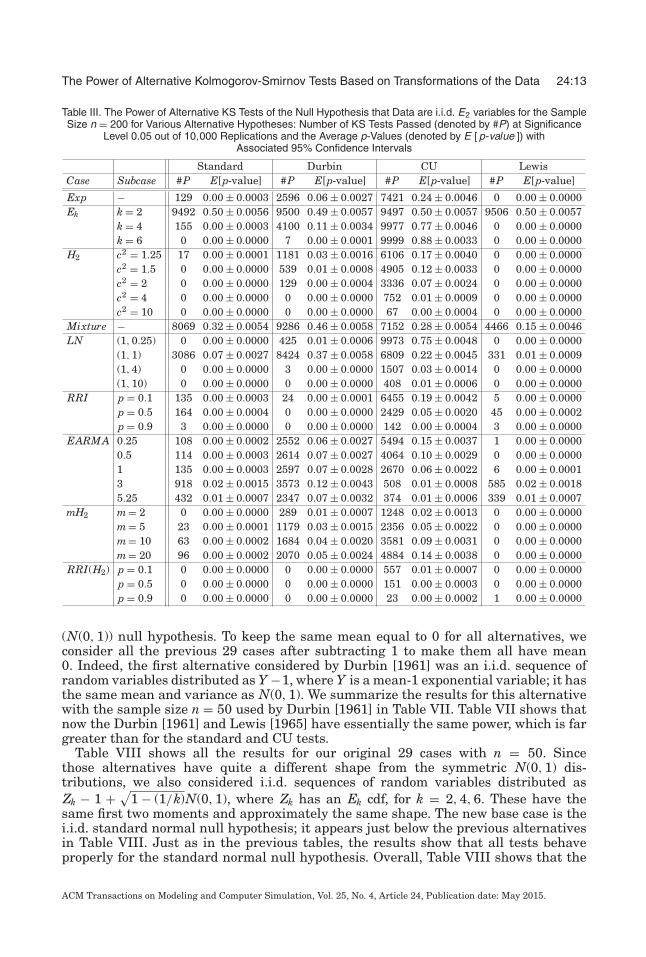
We now consider three different i.i.d. null hypotheses: E2, H2 with c2 = 2, and LN(1, 4);lognormal hypotheses are especially interesting for service systems, for example, Brownet al. [2005]. The results are shown for the same 29 cases in the following Tables III–Vfor the base case of n = 200. As before, all tests perform properly for the null hy-potheses. The ordering of the tests by power when we consider the i.i.d. exponentialalternative hypothesis is the same as before. Overall, these tables show that the pre-vious conclusions for the i.i.d. exponential null hypothesis conclusions extend to i.i.d.null hypotheses with other marginal cdfs.

As with the exponential null hypothesis, the Durbin test performs especially wellfor the RRI, because the repetitions are converted to 0’s, but for these other nullhypotheses, the standard and Lewis tests have almost equal power.

5.4. Larger Sample Sizes

Tables II–V clearly show how the power decreases as the alternative gets closer to thei.i.d. null hypothesis. For the i.i.d. exponential null hypothesis and the i.i.d. alternativehypotheses, we see this as the scv c2

X approaches 1; for the dependent exponentialsequences, we see this as the degree of dependence decreases. However, all of these arefor the sample size n = 200. The power also increases as we increase the sample size, aswe now illustrate by considering the case n = 2,000 for the exponential null hypothesisin Table VI. Corresponding results for Erlang, hyperexponential, and lognormal nullhypotheses appear in the online Appendix. When the sample size is increased to n =2,000, all the tests except the CU test reject the alternative hypotheses in all 104

replications for most of the alternatives. Nevertheless, the superiority of the Lewis testfor nonexponential marginals is evident from the H2 case with c2 = 1.25, the superiorityof the Durbin test for the RRI cases is evident, and the superiority of the CU test forthe EARMA cases is evident, consistent with the previous results for n = 200.

6. THE SECOND NORMAL EXPERIMENT

The poor results for the Durbin [1961] test for the i.i.d. cases in Section 5 seem incon-sistent with the results in Durbin [1961] and the enthusiastic endorsement by Lewis[1965], so we decided to repeat some of the experiments actually performed by Durbin[1961]. We now consider the same four KS tests applied to the i.i.d. standard normal



Table III. The Power of Alternative KS Tests of the Null Hypothesis that Data are i.i.d. E2 variables for the SampleSize n = 200 for Various Alternative Hypotheses: Number of KS Tests Passed (denoted by #P) at Significance

Level 0.05 out of 10,000 Replications and the Average p-Values (denoted by E [ p-value ]) withAssociated 95% Confidence Intervals


Exp − 129 0.00 ± 0.0003 2596 0.06 ± 0.0027 7421 0.24 ± 0.0046 0 0.00 ± 0.0000Ek k = 2 9492 0.50 ± 0.0056 9500 0.49 ± 0.0057 9497 0.50 ± 0.0057 9506 0.50 ± 0.0057

k = 4 155 0.00 ± 0.0003 4100 0.11 ± 0.0034 9977 0.77 ± 0.0046 0 0.00 ± 0.0000k = 6 0 0.00 ± 0.0000 7 0.00 ± 0.0001 9999 0.88 ± 0.0033 0 0.00 ± 0.0000

H2 c2 = 1.25 17 0.00 ± 0.0001 1181 0.03 ± 0.0016 6106 0.17 ± 0.0040 0 0.00 ± 0.0000c2 = 1.5 0 0.00 ± 0.0000 539 0.01 ± 0.0008 4905 0.12 ± 0.0033 0 0.00 ± 0.0000c2 = 2 0 0.00 ± 0.0000 129 0.00 ± 0.0004 3336 0.07 ± 0.0024 0 0.00 ± 0.0000c2 = 4 0 0.00 ± 0.0000 0 0.00 ± 0.0000 752 0.01 ± 0.0009 0 0.00 ± 0.0000c2 = 10 0 0.00 ± 0.0000 0 0.00 ± 0.0000 67 0.00 ± 0.0004 0 0.00 ± 0.0000

Mixture − 8069 0.32 ± 0.0054 9286 0.46 ± 0.0058 7152 0.28 ± 0.0054 4466 0.15 ± 0.0046LN (1, 0.25) 0 0.00 ± 0.0000 425 0.01 ± 0.0006 9973 0.75 ± 0.0048 0 0.00 ± 0.0000

(1, 1) 3086 0.07 ± 0.0027 8424 0.37 ± 0.0058 6809 0.22 ± 0.0045 331 0.01 ± 0.0009(1, 4) 0 0.00 ± 0.0000 3 0.00 ± 0.0000 1507 0.03 ± 0.0014 0 0.00 ± 0.0000(1, 10) 0 0.00 ± 0.0000 0 0.00 ± 0.0000 408 0.01 ± 0.0006 0 0.00 ± 0.0000

RRI p = 0.1 135 0.00 ± 0.0003 24 0.00 ± 0.0001 6455 0.19 ± 0.0042 5 0.00 ± 0.0000p = 0.5 164 0.00 ± 0.0004 0 0.00 ± 0.0000 2429 0.05 ± 0.0020 45 0.00 ± 0.0002p = 0.9 3 0.00 ± 0.0000 0 0.00 ± 0.0000 142 0.00 ± 0.0004 3 0.00 ± 0.0000

EARMA 0.25 108 0.00 ± 0.0002 2552 0.06 ± 0.0027 5494 0.15 ± 0.0037 1 0.00 ± 0.00000.5 114 0.00 ± 0.0003 2614 0.07 ± 0.0027 4064 0.10 ± 0.0029 0 0.00 ± 0.00001 135 0.00 ± 0.0003 2597 0.07 ± 0.0028 2670 0.06 ± 0.0022 6 0.00 ± 0.00013 918 0.02 ± 0.0015 3573 0.12 ± 0.0043 508 0.01 ± 0.0008 585 0.02 ± 0.00185.25 432 0.01 ± 0.0007 2347 0.07 ± 0.0032 374 0.01 ± 0.0006 339 0.01 ± 0.0007

mH2 m = 2 0 0.00 ± 0.0000 289 0.01 ± 0.0007 1248 0.02 ± 0.0013 0 0.00 ± 0.0000m = 5 23 0.00 ± 0.0001 1179 0.03 ± 0.0015 2356 0.05 ± 0.0022 0 0.00 ± 0.0000m = 10 63 0.00 ± 0.0002 1684 0.04 ± 0.0020 3581 0.09 ± 0.0031 0 0.00 ± 0.0000m = 20 96 0.00 ± 0.0002 2070 0.05 ± 0.0024 4884 0.14 ± 0.0038 0 0.00 ± 0.0000

RRI(H2) p = 0.1 0 0.00 ± 0.0000 0 0.00 ± 0.0000 557 0.01 ± 0.0007 0 0.00 ± 0.0000p = 0.5 0 0.00 ± 0.0000 0 0.00 ± 0.0000 151 0.00 ± 0.0003 0 0.00 ± 0.0000p = 0.9 0 0.00 ± 0.0000 0 0.00 ± 0.0000 23 0.00 ± 0.0002 1 0.00 ± 0.0000

(N(0, 1)) null hypothesis. To keep the same mean equal to 0 for all alternatives, weconsider all the previous 29 cases after subtracting 1 to make them all have mean0. Indeed, the first alternative considered by Durbin [1961] was an i.i.d. sequence ofrandom variables distributed as Y −1, where Y is a mean-1 exponential variable; it hasthe same mean and variance as N(0, 1). We summarize the results for this alternativewith the sample size n = 50 used by Durbin [1961] in Table VII. Table VII shows thatnow the Durbin [1961] and Lewis [1965] have essentially the same power, which is fargreater than for the standard and CU tests.

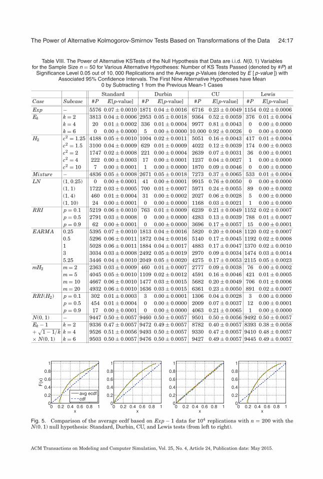
Table VIII shows all the results for our original 29 cases with n = 50. Sincethose alternatives have quite a different shape from the symmetric N(0, 1) dis-tributions, we also considered i.i.d. sequences of random variables distributed asZk − 1 +

√1 − (1/k)N(0, 1), where Zk has an Ek cdf, for k = 2, 4, 6. These have the

same first two moments and approximately the same shape. The new base case is thei.i.d. standard normal null hypothesis; it appears just below the previous alternativesin Table VIII. Just as in the previous tables, the results show that all tests behaveproperly for the standard normal null hypothesis. Overall, Table VIII shows that the



Table IV. The Power of Alternative KS Tests of the Null Hypothesis that Data are i.i.d. H2 with c2 = 2 Variables forthe Sample Size n = 200 for Various Alternative Hypotheses: Number of KS Tests Passed (denoted by #P) atSignificance Level 0.05 out of 10,000 Replications and the Average p-Values (denoted by E [ p-value ]) with

Associated 95% Confidence Intervals


Exp − 3661 0.10 ± 0.0034 8951 0.43 ± 0.0058 9935 0.69 ± 0.0051 1613 0.03 ± 0.0014Ek k = 2 0 0.00 ± 0.0000 92 0.00 ± 0.0003 10000 0.89 ± 0.0032 0 0.00 ± 0.0000

k = 4 0 0.00 ± 0.0000 0 0.00 ± 0.0000 10000 0.98 ± 0.0012 0 0.00 ± 0.0000k = 6 0 0.00 ± 0.0000 0 0.00 ± 0.0000 10000 0.99 ± 0.0005 0 0.00 ± 0.0000

H2 c2 = 1.25 6574 0.23 ± 0.0052 9433 0.49 ± 0.0057 9850 0.63 ± 0.0055 5543 0.15 ± 0.0038c2 = 1.5 8530 0.39 ± 0.0059 9497 0.50 ± 0.0057 9750 0.58 ± 0.0056 8307 0.34 ± 0.0055c2 = 2 9511 0.50 ± 0.0056 9482 0.50 ± 0.0057 9482 0.50 ± 0.0057 9507 0.50 ± 0.0056c2 = 4 4983 0.14 ± 0.0040 9107 0.44 ± 0.0058 8143 0.31 ± 0.0052 3888 0.11 ± 0.0038c2 = 10 269 0.01 ± 0.0005 6142 0.19 ± 0.0046 5098 0.15 ± 0.0039 1221 0.04 ± 0.0024

Mixture − 0 0.00 ± 0.0000 1932 0.04 ± 0.0021 9989 0.80 ± 0.0043 0 0.00 ± 0.0000LN (1, 0.25) 0 0.00 ± 0.0000 0 0.00 ± 0.0000 10000 0.98 ± 0.0011 0 0.00 ± 0.0000

(1, 1) 0 0.00 ± 0.0000 585 0.01 ± 0.0006 9982 0.77 ± 0.0046 0 0.00 ± 0.0000(1, 4) 5685 0.18 ± 0.0045 9051 0.44 ± 0.0059 8493 0.36 ± 0.0055 5281 0.16 ± 0.0043(1, 10) 13 0.00 ± 0.0001 4888 0.15 ± 0.0043 5824 0.17 ± 0.0042 11 0.00 ± 0.0001

RRI p = 0.1 3400 0.09 ± 0.0032 1352 0.02 ± 0.0010 9804 0.61 ± 0.0056 1410 0.03 ± 0.0013p = 0.5 2058 0.05 ± 0.0020 0 0.00 ± 0.0000 7608 0.28 ± 0.0050 883 0.02 ± 0.0012p = 0.9 9 0.00 ± 0.0001 0 0.00 ± 0.0000 1282 0.03 ± 0.0017 6 0.00 ± 0.0000

EARMA 0.25 3697 0.10 ± 0.0035 8922 0.43 ± 0.0058 9684 0.56 ± 0.0056 1577 0.03 ± 0.00140.5 3839 0.11 ± 0.0037 8872 0.42 ± 0.0059 9216 0.45 ± 0.0057 1630 0.03 ± 0.00151 3755 0.11 ± 0.0037 8629 0.40 ± 0.0059 8364 0.34 ± 0.0055 1607 0.03 ± 0.00173 3607 0.13 ± 0.0044 5683 0.19 ± 0.0047 3333 0.08 ± 0.0028 2577 0.07 ± 0.00325.25 2770 0.08 ± 0.0032 6642 0.27 ± 0.0056 3118 0.08 ± 0.0029 1690 0.05 ± 0.0025

mH2 m = 2 8771 0.42 ± 0.0058 9466 0.49 ± 0.0057 7788 0.29 ± 0.0052 9091 0.43 ± 0.0057m = 5 6227 0.24 ± 0.0053 9290 0.47 ± 0.0058 7974 0.33 ± 0.0056 5465 0.16 ± 0.0041m = 10 5052 0.18 ± 0.0047 9032 0.44 ± 0.0058 8543 0.40 ± 0.0061 3210 0.07 ± 0.0025m = 20 4598 0.15 ± 0.0044 9013 0.43 ± 0.0058 9265 0.50 ± 0.0061 2263 0.05 ± 0.0018

RRI(H2) p = 0.1 4641 0.14 ± 0.0040 1227 0.02 ± 0.0010 7377 0.26 ± 0.0048 3720 0.11 ± 0.0037p = 0.5 2542 0.05 ± 0.0022 0 0.00 ± 0.0000 3586 0.09 ± 0.0029 2467 0.05 ± 0.0022p = 0.9 13 0.00 ± 0.0001 0 0.00 ± 0.0000 440 0.01 ± 0.0008 9 0.00 ± 0.0001

Durbin [1961] test performs much better now, just as originally reported. In this caseboth the Durbin [1961] and Lewis [1965] KS tests perform much better than the stan-dard and CU alternatives. An exception is the set of three modified Erlang cases, withthe same shape and first two moments as N(0, 1). The Lewis test has the most power,but all four tests have low power for these cases.

As in Section 5, the power increases as the sample size increases; see the Appendixfor the test results for the larger sample size n = 200. In that case, we observe thatall tests except CU have estimated perfect power except in the last three modifiedErlang cases, where the Lewis test stands out with power 0.375 for the modified E2case compared to 0.130 for standard and CU, and only 0.055 for Durbin. Figures 5 and6 show that the reason can be seen in the average of the ecdfs of the transformed data.

7. ESTIMATING PARAMETERS

The KS test assumes a fully specified cdf, which is rarely the case in applications. Inthis section we investigate the consequence of having to estimate the parameters ofthe cdf in the null hypothesis. Before doing so, we observe that there is one case in



Table V. The Power of Alternative KS Tests of the Null Hypothesis that Data are i.i.d. LN(1, 4) Variables for theSample Size n = 200 for Various Alternative Hypotheses: Number of KS Tests Passed (denoted by #P) at

Significance Level 0.05 out of 10,000 Replications and the Average p-Values (denoted by E [ p-value ]) withAssociated 95% Confidence Intervals


Exp − 181 0.00 ± 0.0005 5509 0.18 ± 0.0046 9972 0.75 ± 0.0047 38 0.00 ± 0.0002Ek k = 2 0 0.00 ± 0.0000 0 0.00 ± 0.0000 10000 0.93 ± 0.0024 0 0.00 ± 0.0000

k = 4 0 0.00 ± 0.0000 0 0.00 ± 0.0000 10000 0.99 ± 0.0007 0 0.00 ± 0.0000k = 6 0 0.00 ± 0.0000 0 0.00 ± 0.0000 10000 1.00 ± 0.0003 0 0.00 ± 0.0000

H2 c2 = 1.25 811 0.02 ± 0.0012 7382 0.29 ± 0.0056 9939 0.70 ± 0.0051 513 0.01 ± 0.0007c2 = 1.5 2340 0.05 ± 0.0023 8354 0.37 ± 0.0058 9895 0.66 ± 0.0053 2255 0.05 ± 0.0020c2 = 2 5665 0.17 ± 0.0043 9006 0.43 ± 0.0058 9788 0.59 ± 0.0055 6140 0.19 ± 0.0043c2 = 4 9164 0.36 ± 0.0048 8864 0.41 ± 0.0058 9294 0.46 ± 0.0056 8783 0.31 ± 0.0046c2 = 10 3774 0.08 ± 0.0023 6700 0.23 ± 0.0050 8538 0.35 ± 0.0054 5450 0.13 ± 0.0032

Mixture − 0 0.00 ± 0.0000 196 0.00 ± 0.0005 10,000 0.87 ± 0.0034 0 0.00 ± 0.0000LN (1, 0.25) 0 0.00 ± 0.0000 0 0.00 ± 0.0000 10,000 0.99 ± 0.0005 0 0.00 ± 0.0000

(1, 1) 0 0.00 ± 0.0000 90 0.00 ± 0.0003 9999 0.85 ± 0.0037 0 0.00 ± 0.0000(1, 4) 9508 0.50 ± 0.0056 9508 0.50 ± 0.0056 9508 0.50 ± 0.0057 9490 0.50 ± 0.0057(1, 10) 232 0.01 ± 0.0005 6261 0.22 ± 0.0051 8094 0.30 ± 0.0051 185 0.00 ± 0.0004

RRI p = 0.1 193 0.00 ± 0.0005 346 0.01 ± 0.0004 9921 0.68 ± 0.0053 47 0.00 ± 0.0001p = 0.5 408 0.01 ± 0.0007 0 0.00 ± 0.0000 8255 0.34 ± 0.0054 120 0.00 ± 0.0003p = 0.9 13 0.00 ± 0.0001 0 0.00 ± 0.0000 1738 0.04 ± 0.0021 3 0.00 ± 0.0001

EARMA 0.25 206 0.00 ± 0.0006 5443 0.18 ± 0.0046 9866 0.64 ± 0.0054 34 0.00 ± 0.00010.5 312 0.01 ± 0.0007 5388 0.17 ± 0.0045 9571 0.53 ± 0.0058 44 0.00 ± 0.00021 436 0.01 ± 0.0009 5032 0.16 ± 0.0045 9023 0.43 ± 0.0058 72 0.00 ± 0.00033 1594 0.04 ± 0.0024 4073 0.13 ± 0.0041 4018 0.10 ± 0.0033 647 0.01 ± 0.00125.25 1220 0.03 ± 0.0019 3612 0.12 ± 0.0042 4027 0.11 ± 0.0036 469 0.01 ± 0.0013

mH2 m = 2 4930 0.15 ± 0.0040 8640 0.39 ± 0.0058 8786 0.39 ± 0.0057 4425 0.12 ± 0.0035m = 5 1706 0.04 ± 0.0022 7193 0.27 ± 0.0055 8677 0.40 ± 0.0059 606 0.01 ± 0.0008m = 10 1083 0.03 ± 0.0017 6179 0.22 ± 0.0051 9085 0.48 ± 0.0062 178 0.00 ± 0.0004m = 20 808 0.02 ± 0.0013 5752 0.19 ± 0.0049 9572 0.57 ± 0.0060 79 0.00 ± 0.0002

RRI(H2) p = 0.1 8581 0.29 ± 0.0046 834 0.02 ± 0.0008 8830 0.39 ± 0.0055 8117 0.26 ± 0.0044p = 0.5 3857 0.08 ± 0.0024 0 0.00 ± 0.0000 5080 0.14 ± 0.0036 3547 0.07 ± 0.0024p = 0.9 17 0.00 ± 0.0001 0 0.00 ± 0.0000 658 0.01 ± 0.0010 5 0.00 ± 0.0001

which we do not need to estimate any parameters. That fortunate situation occurs withexponential cdfs. Exponential cdfs can be regarded as the interarrival times of a PPwith a rate equal to the reciprocal of its mean. However, we do not need to know thatmean, because the conditional-uniform transformation is independent of the rate ofthe PP. Thus, the new KS tests of an i.i.d. sequence with an exponential cdf that exploitthe CU property have the advantage that they do not require estimating the mean.

Having to estimate the parameters can have a big influence. For example, in Kimand Whitt [2014b] (see Section 6 of its online Appendix [Kim and Whitt 2014c] forfurther details), we found that in a standard KS test of a mean-1 exponential cdf, if weuse the KS test with the estimated mean and act as if it is the known mean, then itis necessary to increase the nominal significance level from 0.05 to 0.18 with a samplesize of n = 200 in order for the actual significance level to be α = 0.05. The resultingstatistical test with estimated mean then coincides with the Lilliefors [1969] test.

To examine the impact of estimating the parameters, we consider testing for lognor-mal and normal distributions with estimated parameters, using the maximum like-lihood estimators. (See Section F of the Appendix for further information on how weestimated the parameters and selected the nominal significance levels.) The nominal



Table VI. The Power of Alternative KS Tests of the Null Hypothesis that Data are i.i.d. Mean-1 ExponentialVariables for the Sample Sze n = 2,000 for Various Alternative Hypotheses: Number of KS Tests Passed

(denoted by #P) at Significance Level 0.05 out of 10,000 Replications and the Average p-Values (denoted byE [ p-value ]) with Associated 95% Confidence Intervals


Exp − 9515 0.50 ± 0.0056 9495 0.50 ± 0.0057 9481 0.50 ± 0.0057 9495 0.50 ± 0.0057Ek k = 2 0 0.00 ± 0.0000 0 0.00 ± 0.0000 9985 0.79 ± 0.0044 0 0.00 ± 0.0000

k = 4 0 0.00 ± 0.0000 0 0.00 ± 0.0000 10,000 0.95 ± 0.0019 0 0.00 ± 0.0000k = 6 0 0.00 ± 0.0000 0 0.00 ± 0.0000 10,000 0.98 ± 0.0009 0 0.00 ± 0.0000

H2 c2 = 1.25 3380 0.08 ± 0.0029 9360 0.48 ± 0.0057 8957 0.40 ± 0.0055 281 0.01 ± 0.0006c2 = 1.5 68 0.00 ± 0.0002 8320 0.36 ± 0.0059 8313 0.32 ± 0.0051 0 0.00 ± 0.0000c2 = 2 0 0.00 ± 0.0000 3425 0.08 ± 0.0030 6893 0.21 ± 0.0043 0 0.00 ± 0.0000c2 = 4 0 0.00 ± 0.0000 0 0.00 ± 0.0000 2788 0.05 ± 0.0019 0 0.00 ± 0.0000c2 = 10 0 0.00 ± 0.0000 0 0.00 ± 0.0000 34 0.00 ± 0.0002 0 0.00 ± 0.0000

Mixture − 0 0.00 ± 0.0000 4 0.00 ± 0.0001 9450 0.52 ± 0.0058 0 0.00 ± 0.0000LN (1, 0.25) 0 0.00 ± 0.0000 0 0.00 ± 0.0000 10,000 0.95 ± 0.0019 0 0.00 ± 0.0000

(1, 1) 0 0.00 ± 0.0000 0 0.00 ± 0.0000 9501 0.51 ± 0.0057 0 0.00 ± 0.0000(1, 4) 0 0.00 ± 0.0000 0 0.00 ± 0.0000 2610 0.06 ± 0.0023 0 0.00 ± 0.0000(1, 10) 0 0.00 ± 0.0000 0 0.00 ± 0.0000 242 0.00 ± 0.0005 0 0.00 ± 0.0000

RRI p = 0.1 9010 0.41 ± 0.0055 0 0.00 ± 0.0000 9129 0.41 ± 0.0055 9014 0.40 ± 0.0055p = 0.5 4410 0.10 ± 0.0028 0 0.00 ± 0.0000 4666 0.11 ± 0.0030 4531 0.10 ± 0.0028p = 0.9 0 0.00 ± 0.0000 0 0.00 ± 0.0000 25 0.00 ± 0.0001 0 0.00 ± 0.0000

EARMA 0.25 9336 0.47 ± 0.0057 9483 0.50 ± 0.0057 8326 0.33 ± 0.0052 9429 0.49 ± 0.00570.5 8806 0.42 ± 0.0059 9505 0.50 ± 0.0057 7063 0.22 ± 0.0044 9408 0.49 ± 0.00571 8210 0.37 ± 0.0059 9488 0.50 ± 0.0057 4722 0.12 ± 0.0031 8901 0.43 ± 0.00583 5247 0.21 ± 0.0054 6406 0.22 ± 0.0049 822 0.01 ± 0.0008 6715 0.29 ± 0.00615.25 4111 0.14 ± 0.0045 9290 0.47 ± 0.0058 193 0.00 ± 0.0003 5769 0.21 ± 0.0051

mH2 m = 2 0 0.00 ± 0.0000 5272 0.16 ± 0.0042 3029 0.06 ± 0.0022 0 0.00 ± 0.0000m = 5 3135 0.09 ± 0.0032 9281 0.46 ± 0.0058 3434 0.07 ± 0.0024 182 0.00 ± 0.0004m = 10 6428 0.25 ± 0.0054 9471 0.49 ± 0.0057 3732 0.09 ± 0.0027 4432 0.13 ± 0.0040m = 20 7364 0.31 ± 0.0058 9470 0.50 ± 0.0057 4365 0.11 ± 0.0033 8127 0.35 ± 0.0058

RRI(H2) p = 0.1 0 0.00 ± 0.0000 0 0.00 ± 0.0000 1897 0.03 ± 0.0015 0 0.00 ± 0.0000p = 0.5 0 0.00 ± 0.0000 0 0.00 ± 0.0000 177 0.00 ± 0.0003 0 0.00 ± 0.0000p = 0.9 0 0.00 ± 0.0000 0 0.00 ± 0.0000 0 0.00 ± 0.0000 0 0.00 ± 0.0000

Table VII. The Power of Alternative KS Tests of the Null Hypothesis that Data arei.i.d. Standard Normal N(0, 1) Variables for the Sample Size n = 50 with Significance

Level α = 0.05: The Alternative Hypothesis of i.i.d. Random Variables Distributedas Y − 1, where Y is a Mean-1 Exponential Random Variable

KS test Lewis Standard CU DurbinPower 0.885 0.443 0.328 0.813Average p-value 0.02 0.07 0.23 0.04

significance level had to be increased from 0.05 to 0.38 for the Standard test andto 0.16 for the Lewis test in order for the actual significance level to be α = 0.05.Tables IX–XI provide the test results.

The four lognormal distributions with different variances can each be regarded asthe null hypothesis when the KS tests of a lognormal null hypothesis are applied withestimated parameters, because they will have the appropriate estimated parameters.Table IX for n = 200 and Table X for n = 2,000 shows that, after the adjustmentsdescribed earlier, they all have the correct significance level. Comparing Table IX toTable V, we see that the relative performance of the four KS tests is about the same: The



Table VIII. The Power of Alternative KSTests of the Null Hypothesis that Data are i.i.d. N(0, 1) Variablesfor the Sample Size n = 50 for Various Alternative Hypotheses: Number of KS Tests Passed (denoted by #P) at

Significance Level 0.05 out of 10, 000 Replications and the Average p-Values (denoted by E [ p-value ]) withAssociated 95% Confidence Intervals. The First Nine Alternative Hypotheses have Mean

0 by Subtracting 1 from the Previous Mean-1 Cases


Exp − 5576 0.07 ± 0.0010 1871 0.04 ± 0.0016 6716 0.23 ± 0.0049 1154 0.02 ± 0.0006Ek k = 2 3813 0.04 ± 0.0006 2953 0.05 ± 0.0018 9364 0.52 ± 0.0059 376 0.01 ± 0.0004

k = 4 20 0.01 ± 0.0002 336 0.01 ± 0.0004 9977 0.81 ± 0.0043 0 0.00 ± 0.0000k = 6 0 0.00 ± 0.0000 5 0.00 ± 0.0000 10,000 0.92 ± 0.0026 0 0.00 ± 0.0000

H2 c2 = 1.25 4188 0.05 ± 0.0010 1004 0.02 ± 0.0011 5051 0.16 ± 0.0043 417 0.01 ± 0.0004c2 = 1.5 3100 0.04 ± 0.0009 629 0.01 ± 0.0009 4022 0.12 ± 0.0039 174 0.00 ± 0.0003c2 = 2 1747 0.02 ± 0.0008 221 0.00 ± 0.0004 2639 0.07 ± 0.0031 36 0.00 ± 0.0001c2 = 4 222 0.00 ± 0.0003 17 0.00 ± 0.0001 1237 0.04 ± 0.0027 1 0.00 ± 0.0000c2 = 10 7 0.00 ± 0.0001 1 0.00 ± 0.0000 1870 0.09 ± 0.0046 0 0.00 ± 0.0000

Mixture − 4836 0.05 ± 0.0008 2671 0.05 ± 0.0018 7273 0.37 ± 0.0065 533 0.01 ± 0.0004LN (1, 0.25) 0 0.00 ± 0.0001 41 0.00 ± 0.0001 9915 0.76 ± 0.0050 0 0.00 ± 0.0000

(1, 1) 1722 0.03 ± 0.0005 700 0.01 ± 0.0007 5971 0.24 ± 0.0055 89 0.00 ± 0.0002(1, 4) 460 0.01 ± 0.0004 31 0.00 ± 0.0002 2027 0.06 ± 0.0028 5 0.00 ± 0.0000(1, 10) 24 0.00 ± 0.0001 0 0.00 ± 0.0000 1168 0.03 ± 0.0021 1 0.00 ± 0.0000

RRI p = 0.1 5219 0.06 ± 0.0010 763 0.01 ± 0.0009 6239 0.21 ± 0.0049 1152 0.02 ± 0.0007p = 0.5 2791 0.03 ± 0.0008 0 0.00 ± 0.0000 4283 0.13 ± 0.0039 788 0.01 ± 0.0007p = 0.9 62 0.00 ± 0.0001 0 0.00 ± 0.0000 3696 0.17 ± 0.0057 15 0.00 ± 0.0001

EARMA 0.25 5395 0.07 ± 0.0010 1813 0.04 ± 0.0016 5820 0.20 ± 0.0048 1120 0.02 ± 0.00070.5 5296 0.06 ± 0.0011 1872 0.04 ± 0.0016 5140 0.17 ± 0.0045 1192 0.02 ± 0.00081 5028 0.06 ± 0.0011 1884 0.04 ± 0.0017 4883 0.17 ± 0.0047 1370 0.02 ± 0.00103 3034 0.03 ± 0.0008 2492 0.05 ± 0.0019 2970 0.09 ± 0.0034 1474 0.03 ± 0.00145.25 3446 0.04 ± 0.0010 2049 0.05 ± 0.0020 4275 0.17 ± 0.0053 2115 0.05 ± 0.0023

mH2 m = 2 2363 0.03 ± 0.0009 460 0.01 ± 0.0007 2777 0.09 ± 0.0038 76 0.00 ± 0.0002m = 5 4045 0.05 ± 0.0010 1109 0.02 ± 0.0012 4591 0.16 ± 0.0046 421 0.01 ± 0.0005m = 10 4667 0.06 ± 0.0010 1477 0.03 ± 0.0015 5682 0.20 ± 0.0049 706 0.01 ± 0.0006m = 20 4932 0.06 ± 0.0010 1636 0.03 ± 0.0015 6361 0.23 ± 0.0050 891 0.02 ± 0.0007

RRI(H2) p = 0.1 302 0.01 ± 0.0003 3 0.00 ± 0.0001 1306 0.04 ± 0.0028 3 0.00 ± 0.0000p = 0.5 454 0.01 ± 0.0004 0 0.00 ± 0.0000 2009 0.07 ± 0.0037 12 0.00 ± 0.0001p = 0.9 17 0.00 ± 0.0001 0 0.00 ± 0.0000 4063 0.21 ± 0.0065 1 0.00 ± 0.0000

N(0, 1) − 9447 0.50 ± 0.0057 9460 0.50 ± 0.0057 9501 0.50 ± 0.0056 9492 0.50 ± 0.0057Ek − 1 k = 2 9336 0.47 ± 0.0057 9472 0.49 ± 0.0057 8782 0.40 ± 0.0057 8393 0.38 ± 0.0058+ √

1 − 1/k k = 4 9526 0.51 ± 0.0056 9493 0.50 ± 0.0057 9330 0.47 ± 0.0057 9410 0.48 ± 0.0057× N(0, 1) k = 6 9503 0.50 ± 0.0057 9476 0.50 ± 0.0057 9427 0.49 ± 0.0057 9445 0.49 ± 0.0057

Fig. 5. Comparison of the average ecdf based on Exp − 1 data for 104 replications with n = 200 with theN(0, 1) null hypothesis: Standard, Durbin, CU, and Lewis tests (from left to right).



Table IX. Performance of Alternative KS Tests of i.i.d. Lognormal Variables with Estimated Mean and Variancefor the Sample Size n = 200: Number of KS Tests Passed at Significance Level 0.05 out of 10,000 ReplicationsThe nominal significance levels are increased from 0.05 to 0.38 for the Standard test and to 0.16 for the Lewistest in order for the actual significance level to be 0.05.

Case Subcase Standard Durbin CU Lewis

Exp − 432 7238 9950 46Ek k = 2 2712 9001 9896 1030

k = 4 5782 9381 9833 3858k = 6 7027 9427 9781 5636

H2 c2 = 1.25 926 8152 9931 197c2 = 1.5 1716 8689 9915 598c2 = 2 2616 9121 9877 1467c2 = 4 3358 9036 9695 2823c2 = 10 1607 7609 9496 1503

Mixture − 1182 8049 9888 483LN (1, 0.25) 9497 9496 9493 9454

(1, 1) 9501 9525 9505 9477(1, 4) 9535 9519 9516 9530(1, 10) 9499 9479 9505 9484

RRI p = 0.1 396 638 9872 61p = 0.5 223 0 7823 123p = 0.9 0 0 830 2

EARMA 0.25 435 7313 9795 410.5 384 7214 9440 331 432 7033 8721 613 2606 5846 2862 13695.25 712 5716 3318 223

mH2 m = 2 1952 8888 9008 950m = 5 959 8145 8604 228m = 10 653 7728 8917 114m = 20 460 7517 9448 63

RRI(H2) p = 0.1 2874 1173 9437 2644p = 0.5 1041 0 6128 1408p = 0.9 1 0 463 4

Fig. 6. Comparison of the average ecdf based on E2 − 1 + √1 − 1/kN(0, 1) data for 104 replications and

n = 200 with the N(0, 1) null hypothesis: Standard, Durbin, CU, and Lewis tests (from left to right).

Lewis KS test is best, with the standard KS test close behind, and both significantlybetter than the other two.

We also find that the relative performance of the KS tests of the normal null hy-pothesis when we estimate parameters is about the same as for specified parameters.Table XI shows the results for n = 50. Comparing Table XI to Table VIII, we see thatin some cases the parameter estimation causes a loss in power, but the degradationis least for the Lewis KS test. As in Section 6, we consider i.i.d. sequences of random



Table X. Performance of Alternative KS Tests of i.i.d. Lognormal Variables with Estimated Mean and Variance forthe Sample Size n = 2,000: Number of KS Tests Passed at Significance Level 0.05 out of 10,000 Replications

The nominal significance levels are increased from 0.05 to 0.38 for the Standard test and to 0.16 for the Lewistest in order for the actual significance level to be 0.05.


Exp − 0 28 9968 0Ek k = 2 0 3214 9907 0

k = 4 0 7743 9838 0k = 6 24 8744 9805 0

H2 c2 = 1.25 0 510 9955 0c2 = 1.5 0 1857 9922 0c2 = 2 0 4445 9870 0c2 = 4 0 4774 9693 0c2 = 10 0 267 9422 0

Mixture − 0 675 9889 0LN (1, 0.25) 9522 9496 9521 9500

(1, 1) 9506 9477 9512 9494(1, 4) 9455 9513 9517 9452(1, 10) 9482 9494 9483 9488

RRI p = 0.1 0 0 9892 0p = 0.5 0 0 7717 0p = 0.9 0 0 203 0

EARMA 0.25 0 22 9797 00.5 0 36 9351 01 0 21 8295 03 0 575 2272 05.25 0 95 1322 0

mH2 m = 2 0 3325 8834 0m = 5 0 625 7830 0m = 10 0 160 7522 0m = 20 0 62 7694 0

RRI(H2) p = 0.1 0 0 9445 0p = 0.5 0 0 5555 0p = 0.9 0 0 43 0

variables distributed as Ek − 1 +√

1 − (1/k)N(0, 1) for k = 2, 4, 6, which have the samefirst two moments and approximately the same shape as N(0, 1). For this relativelychallenging example, we see from Tables VIII and XI that the Lewis KS test has greaterpower than for known parameters, and outperforms the other KS tests. Similar resultsfor n = 200 can be found in the Appendix.

8. CONCLUSIONS

We have conducted simulation experiments to study the power of alternative KS sta-tistical tests of the null hypothesis that observations come from a sequence if i.i.d.random variables with continuous cdf F, focusing on the exponential and standardnormal null hypotheses. Our analysis strongly supports the data-transformation ap-proach proposed by Durbin [1961] for the normal null hypothesis, but we find that itperforms poorly for the exponential distribution and related distributions of nonnega-tive random variables.

Our main conclusion is that a new KS test, involving a new combination of trans-formations, has more power. In particular, we find that it is better to transform thegiven hypothesized sequence to i.i.d. exponential random variables (under the null



Table XI. Performance of Alternative KS Tests of i.i.d. Normal Variables with Estimated Mean and Variance forthe Sample Size n = 50: Number of KS Tests Passed at Significance Level 0.05 out of 10,000 Replications

The first nine alternative hypotheses have mean 0 by subtracting 1 from the previous mean-1 cases. (The nominalsignificance levels are increased from 0.05 to 0.38 for the Standard test and to 0.16 for the Lewis test in order forthe actual significance level to be 0.05.)


Exp − 431 2511 6425 170Ek k = 2 3083 7517 7417 1465

k = 4 6063 9185 8168 4001k = 6 7199 9400 8468 5392

H2 c2 = 1.25 141 1293 5490 52c2 = 1.5 58 774 4753 22c2 = 2 21 339 3778 7c2 = 4 14 167 2197 7c2 = 10 68 424 1659 24

Mixture − 2053 5699 5795 925LN (1, 0.25) 3409 8109 7089 1618

(1, 1) 268 2154 5009 80(1, 4) 3 75 3110 0(1, 10) 0 5 2299 0

RRI p = 0.1 464 1161 5785 200p = 0.5 276 0 2962 260p = 0.9 2 0 742 5

EARMA 0.25 482 2663 5272 1800.5 604 2924 4411 2511 924 3456 3819 4403 1668 4500 1244 8965.25 3282 5718 1771 2534

mH2 m = 2 68 667 2826 19m = 5 222 1680 4277 72m = 10 343 2181 5287 117m = 20 380 2419 6046 142

RRI(H2) p = 0.1 26 77 1958 10p = 0.5 54 0 1265 51p = 0.9 1 0 575 4

N(0, 1) − 9489 9477 9516 9437Ek − 1 k = 2 8670 9489 8826 7729+

√1 − (1/k) k = 4 9469 9504 9348 9314

× N(0, 1) k = 6 9526 9465 9439 9415

hypothesis), which can be regarded as the interarrival times of a PP. Then we applythe CU transformation to the PP and afterwards apply the Durbin transformation,as was done by Lewis [1965] in his test of a PP. This new KS test, which we call theLewis test, is usually superior, often markedly so. Thus, we recommend the Lewis test,implemented as described in Section 2.

The Lewis test was found to have more power against alternatives with nonexpo-nential distributions. To test against dependent exponential alternative hypotheses,we recommend also applying the CU KS test. None of the KS tests has much poweragainst dependent exponential alternatives, but the CU KS test seems best.

The realized performance of these different KS tests can be better understood byrecognizing that the CU transformation converts the arrival times into uniform randomvariables, whereas the standard KS test focuses on the interarrival times. The Durbin[1961] transformation is so effective after the CU transformation because it starts by



reordering the interarrival times in ascending order. That explains the performance ofthe CU and Lewis KS tests.

We have observed that the original Durbin KS test has exceptional power againstthe RRI alternative hypotheses and we have explained why. That occurs because therepeated values are converted into 0’s. That repetition structure makes the modelrelatively easy to analyze, but it probably is not often a realistic model of dependence.

Since there is some variation in the results, we recommend applying simulation aswe have done in this article, if there is the opportunity, in order to assess what KStest has the most power and what that power should be in a new setting of interest.The tables and plots based on 104 replications give a very clear picture. As we sawin Section 7, simulation plays an important role in determining the appropriate KStest with estimated parameters. As in the Lilliefors [1969] test of an i.i.d. sequenceof exponential random variables using the estimated mean, it is often necessary toincrease the nominal significance level substantially in order that the KS test withestimated parameters has the final desired significance level. For example, to achievethe target significance level of α = 0.05 in the standard KS test of the exponential nullhypothesis, we found that it is necessary to increase the nominal significance level to0.18.

Both in Kim and Whitt [2014b] and here we have focused on the two-sided KS test,but we also conducted one-sided KS tests. We found that the one-sided test can furtherincrease power when it is justified (see Kim and Whitt [2014c]). As usual with statisticaltests, the power increases with the sample size, so that some sample sizes may be toosmall to have any power, whereas other sample sizes may be too large to accept eventhe slightest deviation from a null hypothesis. Thus, as many have discovered before,judgment is required in the use of statistical tests.

ACKNOWLEDGMENTS

This work was done at Columbia University while Song-Hee Kim was a doctoral student. Support wasreceived from U.S. National Science Foundation grants CMMI 1066372 and 1265070 and by the SamsungFoundation.

REFERENCES

M. Armony, S. Israelit, A. Mandelbaum, Y. Marmor, Y. Tseytlin, and G. Yom-Tov. 2011. Patient Flow inHospitals: A Data-based Queueing-Science Perspective. New York University, http://www.stern.nyu.edu/om/faculty/armony.

G. A. Barnard. 1953. Time Intervals Between Accidents–A Note on Maguire, Pearson & Wynn’s Paper.Biometrika 40 (1953), 212–213.

L. Brown, N. Gans, A. Mandelbaum, A. Sakov, H. Shen, S. Zeltyn, and L. Zhao. 2005. Statistical analysis ofa telephone call center: A queueing-science perspective. J. Am. Stat. Assoc. 100 (2005), 36–50.

M. A. Crane and D. L. Iglehart. 1974a. Simulating stable stochastic systems, I: General multiserver queues.J. ACM 21, 1 (1974), 103–113.

M. A. Crane and D. L. Iglehart. 1974b. Simulating stable stochastic systems, II: Markov chains. J. ACM 23,1 (1974), 114–123.

M. A. Crane and D. L. Iglehart. 1975. Simulating stable stochastic systems: III. Regenerative processes anddiscrete-event simulations. Oper. Res. 23, 1 (1975), 33–45.

J. Durbin. 1961. Some methods for constructing exact tests. Biometrika 48, 1 (1961), 41–55.N. Gans, N. Liu, A. Mandelbaum, H. Shen, and H. Ye. 2010. Service times in call centers: Agent heterogeneity

and learning with some operational consequences. In Borrowing Strength: Theory Powering Applications,A Festschrift for Lawrence D. Brown. Institute of Mathematical Statistics, New York.

P. W. Glynn and D. L. Iglehart. 1989. Importance sampling for stochastic simulations. Manage. Sci. 35, 11(1989), 1367–1392.

P. Heidelberger and D. L. Iglehart. 1979. Comparing stochastic systems using regenerative simulation withcommon random numbers. Adv. Appl. Prob. 11 (1979), 804–819.


http://www.stern.nyu.edu/om/faculty/armony

http://www.stern.nyu.edu/om/faculty/armony


P. A. Jacobs and P. A. W. Lewis. 1977. A Mixed autoregressive-moving average exponential sequence andpoint process (EARMA 1,1). Adv. Appl. Prob. 9, 9 (1977), 87–104.

P. A. Jacobs and P. A. W. Lewis. 1978. Discrete time series generated by mixtures. I: Correlational and runsproperties. J. Roy. Stat. Soc. B 40, 1 (1978), 94–105.

P. A. Jacobs and P. A. W. Lewis. 1983. Stationary autoregressive discrete moving average time series gener-ated by mixtures. J. Roy. Stat. Soc. B 4, 1 (1983), 19–36.

S.-H. Kim and W. Whitt. 2014a. Are call center and hospital arrivals well modeled by nonhomogeneousPoisson processes. Manufact. Service Oper. Manage. 16, 3 (2014), 464–480.

S.-H. Kim and W. Whitt. 2014b. Choosing arrival process models for service systems: Tests of a nonhomoge-neous Poisson process. Nav. Res. Logist. 61, 1 (2014), 66–90.

S.-H. Kim and W. Whitt. 2014c. Choosing Arrival Process Models for Service Systems: Tests of a Non-homogeneous Poisson Process: Appendix. Columbia University. Retrieved from http://www.columbia.edu/∼ww2040/allpapers.html.

S.-H. Kim, P. Vel, W. Whitt, and W. C. Cha. 2015. Poisson and non-Poisson properties in appointment-generated arrival processes: The case of an endocrinology clinic. Operations Research Letters 43 (2015),247–253.

P. A. W. Lewis. 1965. Some results on tests for Poisson processes. Biometrika 52, 1 (1965), 67–77.H. W. Lilliefors. 1969. On the Kolmogorov-Smimov test for the exponential distribution with mean unknown.

J. Am. Statist. Assoc. 64 (1969), 387–389.M. F. Neuts. 1981. Matrix-Geometric Solutions in Stochastic Models: An Algorithmic Approach. The Johns

Hopkins University, Baltimore.G. Pang and W. Whitt. 2012. The impact of dependent service times on large-scale service systems. Manufact.

Service Oper. Manage. 14, 2 (2012), 262–278.S. M. Ross. 1996. Stochastic Processes (2nd. ed.). Wiley, New York.G. R. Shorack and J. A. Wellner. 2009. Empirical Processes with Applications in Statistics (SIAM Classics in

Applied Mathematics ed.). SIAM, Philadelphia.R. Simard and P. L’Ecuyer. 2011. Computing the two-sided Kolmogorov-Smirnov distribution. J. Statist.

Softw. 39, 11 (2011), 1–18.W. Whitt. 1982. Approximating a point process by a renewal process: Two basic methods. Oper. Res. 30 (1982),

125–147.W. Whitt. 2002. Stochastic-Process Limits. Springer, New York.

Received August 2013; revised July 2014; accepted November 2014


http://www.columbia.edu/~ww2040/allpapers.html.

http://www.columbia.edu/~ww2040/allpapers.html.

Documents

The Power of Alternative Kolmogorov-Smirnov Tests Based …ww2040/Kim_Whitt_TOMACS_2015.pdf · The Kolmogorov-Smirnov (KS) statistical test is commonly used to determine if data can