- 1 -

The Intangible Globalization: Explaining the Patterns of

International Trade and FDI in Services

Leo A. Grünfeld* NUPI

(Norwegian Institute of International Affairs )

Andreas Moxnes Department of Economics

University of Oslo

Abstract: Although international trade in services represent more than 20% of worldwide trade, and

trade liberalization within this sector plays a key role in the ongoing WTO negotiations, economists

have devoted surprisingly little attention to the empirical modeling of service trade. In this paper, we

model service trade using a gravity model, based on recently collected bilateral trade and FDI data as

well as indicators for trade barriers, both on macro and more disaggregated levels. We particularly

emphasize the strong links between FDI and international trade in services, since a large proportion of

service trade relates to local supply (Mode 3 trade in the GATS classification).

We provide evidence showing that service trade and FDI are strongly driven by the size and

the similarity in size of the trading partners. The effect of similarity is larger for FDI than for trade,

indicating that multinational enterprises benefit the most when the income of countries converges. This

is consistent with recently developed theoretical models (see e.g. Markusen and Venables, 1998). Our

data on trade barriers and public corruption also contributes to reduce service trade and FDI. However,

when we run regressions based on a more disaggregated data set, the sector specific trade barriers

become less significant. We find that service trade and FDI are complements. We show that an

exporting country fixed effect specification of the gravity model improves the model fit, implying that

there are significant unexplained country specific effects determining service trade. Finally, we predict

the volume of service trade and FDI when barriers are eliminated. The results reveal that there are large

gains from continuing further liberalization efforts, for example via the GATS agreement, but that the

gains from trade are unevenly distributed among countries.

Keywords: Services, International trade, FDI, Gravity models, trade barriers,

JEL classification code: F13, F15, F17, L80

* Corresponding address: NUPI, P.O.Box 8159 Dep. 0033 Oslo, Norway. Tel: (+47) 22056568. Fax: (+47) 22177015. E-mail: leoa.grunfeld@nupi.no URL: http://www.nupi.no

- 2 -

1. Introduction

The composition of global production and trade has changed dramatically over the

last decades. Primary and secondary sectors account for a declining share, while the

relative importance of the tertiary service sectors is growing fast. The rapid

development and deployment of new technology have contributed to strengthen the

importance and volume of international service trade. Communications and

information processing activities have opened new opportunities for cross border

service trade through the Internet and e-commerce. Heavy deregulation of previously

state-controlled service sectors, such as telecommunication and land transport, has

enabled companies to enter new markets outside their home country. Also,

multilateral efforts to liberalize service trade are now taking form through the GATS

and other extensive regional agreements like NATFA and the EU.

Although international trade in services clearly plays an increasingly important role in

the global economy, there is a lack of empirical studies that map the determinants

driving such trade. This comes as no surprise since data availability has been strongly

limited, However, this problem has recently been alleviated as the OECD has started

to publish detailed bilateral service trade figures for its member countries, see OECD

(2002). A second problem that has strong relevance for the empirical study of cross

border service trade is the fact that a large proportion of such trade is mediated

through foreign affiliate sales. According to Karsenty (2000), approximately 40% of

all service trade relates to the activities of foreign subsidiaries, which again requires

some form of service sector FDI. Consequently, the traditional methods for collection

of data on cross border trade in goods are not well suited for mapping trade in

services. To deal with this problem, the UN in cooperation with the EU, IMF, WTO

and the OECD has now published a manual on statistics of international trade in

services (UN, 2002), which describes in detail how countries should collect service

trade data. Unfortunately, only a few countries have initiated programs to follow up

the procedures outlined in the manual.

Impediments to international commodity trade can easily be measured in terms of

trade barriers like tariffs and quotas, but impediments to international trade in services

- 3 -

are more complex and harder to quantify. Here, more diffuse measures like license

requirements, national contents requirements, policies that hinder the movement of

core personnel or the repatriation of profits earned by foreign companies are all

examples of impediments that are hard to quantify, yet strongly relevant for the

service sectors. Nevertheless, a few institutions have recently constructed databases

that contain quantitative indicators mapping impediments to service trade in a large

number of countries. An excellent example is the project administered by the

Australian Productivity Commission1, which is documented by Findlay and Warren

(2000). Furthermore, the World Bank is now finalizing a database on measures

affecting trade in services.

In this paper, we estimate a gravity model that identifies the determinants of

international service trade. We employ recently released data on international trade

and FDI in services, as well as data on the impediments to such trade. We estimate

two models: The first is a gravity model for bilateral exports from the OECD

countries to their trading partners. Here, we find a clear home market effect in service

trade, as the GDP of the exporting country has a stronger impact than the GDP of the

importing country. This is in line with the results derived by Feenstra, Markusen and

Rose (2001) and is consistent with the idea that services are of a highly heterogeneous

nature. Results based on an exporting country fixed effects model show that trade

barriers are detrimental to service trade, but we find no such effect when we look at

service FDI. This is often believed to indicate that impediments to traditional service

trade provide incentives to establish foreign affiliates that supply the foreign market.

However, our study finds that service trade and FDI are complements, which is not

consistent with this story. Moreover, corruption in the importing countries tends to

discourage service trade and FDI, whereas a common membership in a regional free

trade agreement has no significant effect on service trade. This may reflect that many

regional free trade agreements as of today do not emphasize the liberalization of

service trade. Geographical distance is consistently more important for traditional

service exports than for service FDI. Our study shows that the full removal of barriers

to international service trade may increase trade by as much as 50%. Japan, Korea and

the UK will be the largest winners while Northern European countries like Sweden,

1 http://www.pc.gov.au/research/memoranda/servicesrestriction/index.html#book

- 4 -

Norway and Belgium will experience more moderate gains from liberalization (closer

to 30%). However, there are no losers from service liberalization in our sample.

The second model is a gravity model where we employ a 4 year panel of sector

specific Norwegian data on service exports. This data material allows us to take full

advantage of the information contained in the sector specific data on impediments to

service trade. Furthermore, we estimate a 2-stage Heckman model in order to also

take into account observations where there is no export in the data material. This is

important since such observations may indicate a stronger elasticity of trade with

respect to distance, economy size as well as impediments to trade. A standard OLS

regression gives once again support to the negative effect of service trade barriers,

however, when we allow for sector specific fixed effects, the effect of trade barriers

becomes insignificant. This is also the case when we run the 2-stage Heckman model,

and this may indicate that the first and more aggregated model hides important sector

specific information that may alter the empirical results. As outlined above, we find

evidence of significant selection problems in the data set. Moreover, the 2-stage

Heckman model assigns a much stronger effect of both geographical distance and the

size of the importing country. This suggests that future studies of international trade in

service as well as commodities should adjust for selection biases.

The paper is organized as follows. Section 2 gives a brief introduction to the size,

composition and importance of international trade in services. In section 3, we discuss

the gravity model and its relevance for service trade. Here, we briefly review the

earlier literature using gravity models and relate this work to theoretical models.

Section 4 presents data and the model specifications. In section 5 we discuss the

results, while section 6 concludes.

2. The patterns of international service trade There are two important characteristics of services that clearly distinguish trade in

services from trade in goods. First, production and consumption of a service must

appear simultaneously. Communication services are good examples here. Once you

call someone on the phone, the telephone company must instantaneously respond by

producing the requested line connection. One may claim that such services are non-

- 5 -

storable. However, a considerable amount of services, like R&D, business consulting,

literature, film and video services are easily stored and do not demand the outlined

production-consumption simultaneity. Hence, the simultaneity condition is not a

necessary condition for an activity to be characterized as a service. Second, services

have an intangible or non-material nature. That is, services cannot be measured in

traditional volume or metric terms. In his seminal paper «On goods and services», Hill

(1977) defined services as the transformation of already existing goods and

consumers. Here, the production of a movie may serve as a good example. In physical

terms, a movie is only a transformation of an existing, yet empty roll of film. Also,

health services clearly contribute to transform a consumer (patient) by improving her

health condition.

Both the simultaneity condition and the intangible nature of services often require that

suppliers and consumers are physically located at the same place. This is especially so

if the provision of a service rests on the participation of both producers and

consumers, as is the case in education, most kinds of personnel transportation, hair

dressing, restaurant services, retail trade, etc. Furthermore, due to the intangible

nature, the simultaneity condition and the question of geographic proximity, services

are easily differentiable. The same service provided in Oslo and Tokyo is still

different due to location. Moreover, even taxi services provided along the same route

may differ dramatically due to the way it is driven, the way the driver acts and the

quality of the car. Hence, there is a strong element of product heterogeneity in the

supply of services.

According to Tirole (1988), the quality or properties of a good cannot always be

identified before it is purchased or consumed. Tirole labels such goods as experience

goods (quality can only be ascertained after consumption) or credence goods (it is not

possible to identify the level of quality). Apparently, most services are experience

goods, both because production and consumption is performed simultaneously and

because services often are highly differentiated. Consequently, consumers face a

problem of asymmetric information and become the uninformed principal in a moral

hazard situation. In such situation, the service supplier has less incentive to provide a

high quality product. However, if the supplier operates in a market where repeated

purchases are common, the consumer can monitor the service quality over time.

- 6 -

Alternatively, to avoid some of the information disadvantages, consumers can co-

operate by generating systems of reputation regarding service providers. Hence,

reputation becomes one of the most important factors of competition in the service

segment. As Sapir (1991) points out, service producers often become multinational to

be able to follow consumers wherever they have a reputation advantage.

The WTO/GATS classification of service trade modes has now become the ruling

approach to the analysis of international service trade. Four possible modes are

identified:

Mode 1: Cross-border supply of services. Buyer and seller are separated

geographically. Transportation of the service occurs through an electronic network,

for example via phone or email, or, if the service can be embodied in a physical good,

via traditional means of transportation.

Mode 2: Consumers travelling abroad. Here, international tourism and education

services may serve as good examples.

Mode 3: Firms establish a foreign affiliate. This is the traditional way of supplying

business consulting services and financial services. Such trade requires some form of

foreign direct investment (FDI).

Mode 4: The presence of natural persons. In other words, producers travel abroad to

provide the service.

According to Karsenty (2000), mode 1 and mode 3 trade dominate the pattern of

international service trade, where each category represents approximately 40% of total

service trade (see Table 1). Mode 4 trade plays a marginal role and according to the

schedules of the GATS, it is also here we find the strongest barriers to trade.

Table 1: International trade in services by GATS mode classification: 1997 Mode bnUSD % Mode 1 890 41.0% Mode 2 430 19.8% Mode 3 820 37.8% Mode 4 30 1.4% Total 2170 100% Source: Karsenty (2000)

- 7 -

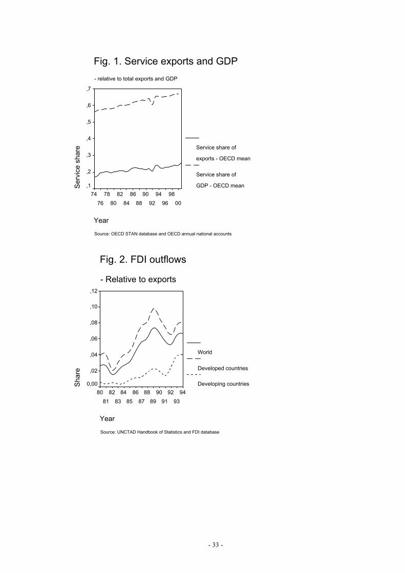
In Figure 1, we plot the service share of GDP and the share of service exports in total

exports for the OECD countries over the period 1974 to 2000. The share of services

in GDP has increased steadily over the whole period and now represents 2/3 of all

economic activity in the OECD area. For the world as a whole, the World Bank

(2001) estimates that service industries contribute to 60 per cent of world GDP. The

share of services in total OECD export rose from 17% in 1974 to 26% in 2001.

Similarly.

Insert Figure 1 here

It is important to recognize that these figures miss a crucial element of overall service

trade, since they only to a limited extent include mode 3 trade through foreign affiliate

sales. Thus, there is reason to claim that that the share of services in total exports is

considerably higher than what is reported in the official statistics. One way to

approach this deficiency is to use FDI as a proxy for foreign affiliate sales. There have

been several studies measuring the aggregate relationship between FDI stocks and

affiliate sales. UNCTAD (1996) estimates that a $1 FDI stock produced $3 in goods

and services in 1993. Petri (97) finds that $1 FDI stock invested in the service sector

generates $1 in service production. USITC (95), which has the most extensive

database on US affiliate sales, finds that, on aggregate, $1 FDI stock in the US service

sector generated $0.6 in sales in the US domestic service market in 1992, however,

their numbers vary considerably when examining the relationship sector by sector.

Figure 2 shows the evolution of the ratio of FDI outflows to exports from 1980 to

1994. Except for a minor decline in 1992, FDI outflows have increased relative to

trade in the whole period. A large share of these FDI flows are related to service trade.

The service share in outward FDI stocks for OECD countries in 1999 was 59.6 %

(OECD International Direct Investment Statistics Yearbook). This indicates that mode

3 trade plays a central role in the overall trade in services and that its role is becoming

ever more important.

Insert figure 2 here.

- 8 -

International statistics clearly show that the relative size of the service sector in a

country is strongly linked to its GDP per capita. Richer countries both have a larger

service sector and a higher share of services in overall exports. This pattern is

illustrated in Figure 3 and is well documented in the earlier literature. The patterns

described in Figure 4 are more surprising. Here, we regress the share of services in

overall imports on services as percent of GDP. The significant negative relationship

illustrates that richer countries have a competitive advantage in service production and

trade, i.e. they export more and import less. This could be a direct consequence of the

fact that these countries have a larger and more developed service sector, providing

services of higher quality.

Insert Figures 3 and 4 here.

3. The gravity model and its relevance for service trade The gravity equation first appeared in the empirical literature with the contributions of

Tinbergen (1962) and Pöyhönen (1963). The standard model is usually specified as

follows:

ijjiijij YYDT Ε= 321 βββ ,

where ijT is trade between country i to j, iY is GDP in country i, ijD represents

distance between the two countries and ijΕ is a regular error term. Distance is usually

interpreted as a proxy for transaction costs. Estimated on a log linear form, the model

often displays an extremely good fit, with a 2R often exceeding 0.80. The income

elasticities are usually found to be in the area around one, while the distance elasticity

is found to be somewhere between –0.9 and –1.5, see e.g. Frankel, 1991 and Learner

1993.

The gravity model for international trade has long been criticized for not having a

clear theoretical basis. Although the model first appeared as a pure empirical

relationship, several theoretical explanations have later appeared in the literature.

Helpman (1987) used the good fit from gravity models as an argument supporting the

new trade theory. Deardorff (1995) showed that the model is consistent with standard

Heckscher-Ohlin-Samuelson (HOS) theory. Moreover, Anderson (1979) developed a

general equilibrium model, assuming differentiated products and CES preferences,

- 9 -

where a reduced-form gravity relationship appears. Thus, economic theory can justify

the gravity model from a multitude of economic perspectives.

On the other hand, there have been no formal attempts to provide a theory that justify

the use of gravity models to predict FDI. Markusen & Venables (1998) however, have

constructed a theory explaining national and foreign affiliate activity as a function of

country income and transport costs. Some of their results are in line with the

predictions of the gravity model. For example, the theory predicts that affiliate sales

increase with income in both the foreign and domestic market, which is also a feature

of the gravity model. Furthermore, the model only considers horizontal FDI. This

feature of the model makes it appealing in relationship to service trade: Vertical FDI

is probably not important in the service segment. In later papers (Carr, Markusen and

Maskus, 2001, Blonigen, 2002), the theories of horizontal and vertical FDI and the

knowledge-capital theory are tested empirically, trying to assess which regime is

consistent with data, and their results give strong support for the horizontal model.

As discussed above, international service trade has some unique properties that make

the gravity modeling appealing. First, the importance of physical proximity between

producer and consumer should give the distance effect a strong boost. Marshall (1987)

examines three geographical regions in the UK and finds that 80% of services

purchased by a local manufacturer are supplied by a firm located in the same region.

Second, service products are often differentiated by quality and location, which may

give rise to monopolistic competition. In a Helpman-Krugman-style “new trade

theory”-model (NTT), these attributes are the driving force behind intra-industry

trade. In the gravity model trade is maximized when ji YY = which is highly

consistent with the predictions of the NTT-model. Helpman (1987) constructed an

econometric specification of the NTT model, quite similar to a gravity specification.

His results gave positive but weak support for the NTT model. Notice however, that

other models such as a HOS-style model or any model with an “Armington” demand

side is compatible with the fact that large income differences produce low trade

(Leamer and Levinsohn, 1995).

- 10 -

Third, we know that the market for services is often characterized by asymmetric

information where reputation and signaling e.g. through marketing play a central role.

Melchior (2002) has expanded the traditional intra industry trade model to include a

mechanism which links market investments (advertising, etc) to trade. The author

assumes that each firm can invest in endogenous sunk costs that will increase demand

for their product. The model predicts that firms will be more export-oriented if their

market investments are not very efficient (does not increase demand much) and if

trade costs are low. If investments are efficient, the presence of transport costs will

increase the total payoff to local investments relative to foreign investments and trade

will decline. In other words, firms become more home market oriented when the

efficiency of the sunk costs increase. How does this result affect the gravity model? If

trade costs increase with distance, the elasticity of exports with respect to distance is

higher in sectors in which fixed market investments are important, such as service

sectors.

Some earlier work

Previous empirical studies have estimated the effects of liberalization on cross-border

trade within a gravity equation framework, often with highly successful results, see

for example Leamer and Levinsohn (1995).

At present, there have not been any previous attempts to use the gravity framework to

estimate the determinants of service trade, measuring both cross-border trade (mode

1) and commercial presence (mode 3). However, there exist studies that examine total

trade and FDI within a gravity framework. Brenton, Di Mauro and Lücke (1998)

assess the impact on bilateral trade and FDI of the deepening integration between the

EU and the CEECs. They apply a gravity model where also population size, income

growth and policy are included. Using a fixed effects specification, they find that

income growth and business-friendly government policies are key determinants of

both FDI and trade. However, they do not find evidence supporting the hypothesis

that the CEECs may increase their trade volume by further integration with the EU. Di

Mauro (2000) contains an econometric study where she attempts to identify the

impact of economic integration on FDI and trade. This is a fixed effects model that

requires that the country specific GDP variables are substituted by a variable

describing the degree of similarity between pairs of countries and a variable

- 11 -

representing the sum of GDP for the two countries. The paper shows that FDI is

mainly horizontal in nature, in the sense that MNEs are motivated by the size and

income similarity of the foreign market and not differences in factor endowments.

Moreover, tariffs have no significant impact on FDI, which implies that tariff-jumping

is not a motivation for MNEs. However, non-tariff barriers do have a negative and

significant impact on FDI. Finally, distance has a significantly negative effect, both on

exports and outgoing FDI stocks.

4. Data and model specification

4.1. The OECD service trade model

A main problem affecting all econometric research in the field of service trade is the

lack of relevant data. However, the surge of increased interest in service trade in

recent years has improved the conditions and our study takes advantage of newly

available data on service trade flows as well as relevant statistics on barriers to such

trade. We estimate the following baseline gravity equations:

(1) 1 2 3 4 5 6ij

ij i j j ij j ijij

td y y cpi FTA tri

fdiα β β β β β β ε

= + + + + + + +

where we use lower case letters since all variables are expressed in logs. The variables

ijt and ijfdi represent bilateral service exports and outgoing FDI stocks from country

i to country j in 1999 respectively. Data on bilateral service exports is taken from the

recently published OECD statistics on international trade in services, OECD (2002),

which covers service exports from 22 OECD countries to their trading partners

(including non-OECD countries).2 Data on bilateral outward FDI stocks are taken

from the OECD International Direct Investment Statistics Yearbook (2002), covering

approximately the same countries. Both variables constitute what is regarded as

service trade by the WTO. Principally, it should be sufficient to only study the trade

variable, however, as argued above there is reason to expect that the statistics on trade

in services collected by the OECD severely underestimates actual service trade since

trade sorting under mode 3 tends to fall out of the data. Since such trade is strongly 2 The data sources are described in detail in the appendix (A.2).

- 12 -

linked to the volume of FDI, we run separate regressions using outward FDI stocks.

One may claim that we conduct separate regressions for mode 1 and 2 trade (tij) and

mode 3 trade (fdiij). However, this is not completely correct since the two

specifications may capture some activity that sorts under other modes. Nevertheless,

the correspondence is rather clear.

The OECD database on FDI stocks does not include bilateral data on service FDI.

Hence we are forced to assume that the ratio of service FDI inflows to total FDI

inflows to a particular host country is identical with respect to every parent country.

To give an example we assume that if 20% of incoming FDI to the US is service

related, than 20% of FDI from Norway to the US is service related. This assumption is

of course a rather crude approximation – obviously the service share might vary

considerably between a particular host and its’ trading partners. Nevertheless, in the

absence of bilateral multi-sector FDI data, this approach is the best available.

The left hand side variables in (1) are as follows: dij represents the geographical

distance between the capital of the exporting and the importing country, yi is GDP in

country i in 1999, cpij is a measure of the level of corruption in country j, based on the

index developed by Transparency International3. FTAij is a dummy variable taking 1

if the two countries i and j are linked through a regional free trade agreement. The

variable trij is a measure of the barriers to service trade in country j.

More on the Trade Restrictiveness Index

Our data on barriers to service trade cover all forms of service trade (i.e. mode 1 to

mode 4 trade) and is taken from the Trade Restrictiveness Index (TRI) database,

developed by the Australian Productivity Commission in cooperation with the

Australian National University4. The database was originally developed by McGuire

and Schuele (2000) for banking services and then applied by Kalirajan (2000),

McGuire et al.(2000) and Nguyen-Hong (2000) for other service sectors. Presently,

the index covers the following sectors: Banking, telecom, maritime services,

distribution (wholesale and retail), education and professional services (engineering,

architectural and legal). The TRI is a pseudo-frequency ratio, which measures market

3 For more information on this index, see www.transparency.org 4 For more information on the TRI index, see http://www.pc.gov.au and Findlay and Warren (2001).

- 13 -

regulations (market access both for domestic and foreign firms, in what is labeled the

‘domestic index’) and protection (exemptions from national treatment, in what is

labeled the ‘foreign index’) for a wide variety of services and countries. The index

contains separate measures for NTBs affecting ongoing operations and NTBs

affecting new establishment of activity. The data is gathered from several different

sources, not just the GATS schedules. Information is taken from APEC, WTO, ITU,

OECD, Tradeport and USTR (Dee, 2001). A TRI listing is constructed as follows:

First, all NTBs affecting a particular sector are counted, then, the different

impediments are assigned weights according to the researchers’ assessment of the

economic impact of the particular NTB.

There are several features and limitations of the index that are worth noting: First, the

TRI is a pseudo-frequency measure, not a tariff equivalent. This means that the index

does not provide information about likely impacts on prices, costs or rates of return in

the economy. In principle, computable general equilibrium (CGE) models will benefit

from using a tariff equivalent, first pioneered by Hockman’s “guessimate” (Hockman,

1995), instead of a frequency index. However, tariff equivalents are difficult to obtain

for service trade, since there is a vast amount of NTBs for every country and each of

them affects the economy differently for each sector.

Second, the TRI does not measure anti-competitive practices (establishment barriers),

like price-fixing, market-sharing arrangements and cartels. These barriers may vary

from country to country, for example, a natural monopoly in Norway might not

appear in the US, due to market size, variable fixed costs, etc. Fink, Matoo and Neago

(2002) argue that private anti-competitive practices in the maritime industry have a

stronger influence on prices than public restrictions. These results suggest that the TRI

might exclude some important aspects of impediments to trade. As noted by Nguyen-

Hong (2000), a higher score may simply reflect a greater availability of information,

rather than a more restrictive regime. This bias may arise when countries do not report

all restrictions to relevant institutions. For example, in the GATS, areas and sectors

that are left out of the schedules might have severe NTBs associated with them.

Third, the indices have only been computed for six industries, which represent

approximately 35 per cent of the 155 sectors covered by Hockman (1995). This is an

- 14 -

important limitation, since our econometric specification examines the effects of tri

on total service trade, not sector specific trade. In econometric terms, this means that

our results might suffer from an omitted variable bias. However, compared to the

Hockman index which is only based on the GATS schedules, the TRI index is much

richer and more detailed, based on a large variety of data sources.

Fourth, we calculate the mean TRI for all countries, giving each industry for which a

TRI is available equal weight. Obviously, this might generate biased results. For

instance, if Austria predominantly imports telecom services, an extraordinarily high

maritime-TRI should not affect trade to a great extent. Ideally, one should weight each

sector specific TRI with an index reflecting the economic importance of imports for

that particular sector, for example, by giving Austria’s telecom TRI a higher weight

than the maritime TRI. Our rationale for choosing the average-TRI approach is first of

all that the sectors covered by the TRI are limited, and second, that the sector specific

TRIs are highly correlated, i.e. a high telecom TRI is usually accompanied by a high

maritime TRI. This means that the average TRI, to a certain extent, captures the

general degree of protection in a country.

Alternative model specifications

The simple gravity model outlined in (1) may suffer from omitted variable bias

because unobservable or unknown country specific effects are left out of the equation.

To deal with this problem, we construct an exporting country fixed-effects model.

However it is not possible to simply apply such a fixed effects regression to model

(1), since the income variables iy and jy are perfectly collinear with the fixed

effects. We deal with this problem by following Egger (2000) and Di Mauro (2000)

who construct the alternative models:

(2) 1 2 3 4 5 6( ) ( )ijji ij ij ij j ij ij

ij

td tgdp sim cpi FTA tri

fdiα ν β β β β β β ε

= + + + + + + + + +

where )ln( jiij YYtgdp += and

+−

+−= 22 )()(1ln

ji

j

ji

iij YY

YYY

Ysim

The variable ijsim is bounded between 0 (absolute divergence in size) and 0.5 (equal

country size). Note what we are not able to include an importing country fixed effect

- 15 -

jν , since this variable is collinear with jtri . We expect that income in both countries

have the same impact on trade as in (1), i.e. economy size increases trade and trade is

maximized when countries have similar income levels.

A closer look at our data reveals that a protectionist regime in the exporting country

seems to reduce exports considerably. Why is this so? A possible explanation is that a

protectionist regime might reduce service exports due to a third variable. For example,

we know that high barriers to imports are correlated with a lower level of skilled

employment and GDP per capita (Holmes and Hardin, 2000), which again is

detrimental to service exports as discussed in section 2. In this context we are

confronted with a spurious relationship between a country’s TRI and exports. An

alternative explanation is that a low exporting country TRI is associated with both

higher exports and imports. We know that many small open economies (for example

Norway) have lower domestic barriers to trade. The reason for this can be twofold:

First, such countries might have a better understanding of the gains from trade.

Second, in the process of bilateral or multilateral liberalization, countries are often

forced to “give something to get something”, i.e. lowering domestic barriers to

acquire access to important foreign markets. This problem justifies an additional

model specification (model 3) where we substitute trij with the sum of trade

restrictions in the exporting and importing country (trii + trij).5

One should expect that corruption in the importing country is detrimental to imports

since it increases trading costs and complicates the distribution and sales of services.

However, exporters that are accustomed to highly corrupt conditions at home should

be less bothered by corruption among its trading partners. Thus, in model 4 we test a

specification where we substitute the cpi index in (2) with the difference in CPI

between the exporting and the importing country.

Finally, since there is a strong relationship between the share of services in total

exports and the relative size of the service sector in the exporting country, one could

claim that our models are miss-specified and that one should rather use service GDP

5 Notice that it is not possible to include a separate variable for exporting country tri in the fixed effects model since this will produce perfect colinearity.

- 16 -

instead of total GDP in the gravity equations.6 This specification error may contribute

to overestimate trade for low-income countries and underestimating trade for high-

income countries. To avoid this problem we substitute the GDP related variables in

(2) with variables based on service sector value added in model 5.

4.2. The sector specific model

As opposed to the OECD statistics on service trade, Norwegian data on service trade

mapping sector specific bilateral trade flows is now available. Statistics Norway

(2002) has now started to collect such data on an annual basis, where exports and

imports of 18 service categories are registered. Out of the 18 service categories, 9

correspond directly with the sector specific trade restrictiveness indexes discussed

above. Hence, the data set allows us to model sector specific effects of barriers to

service trade on a bilateral level. The baseline model takes the following form:

(3) 1 2 3 4js s j j j js jst d y cpi triα κ β β β β ε= + + + + + +

where, tjs is registered service exports of service category s from Norway to country j,

ks represent sector specific fixed effects, dj is the distance from Norway to the

importing country, while the remaining variables are as described above.

Observations on trade and GDP are based on data from 2000. The trade data used in

this exercise contains several observations where there are no exports. This is

important information since it may tell us something about the necessary conditions

for observing exports. In other words, if we disregard the existence of zero-

observations, the econometric model may suffer from selection bias. Earlier

contributions to the modeling of gravity equations rarely deal with this problem,

however, as we shall see, selection bias problems are strongly present when we study

the patterns of service trade. To deal with this problem, we apply a two-stage

Heckman model where the probability of observing export of a service category to a

specific country is estimated in the first stage using a Probit model. In the second

6 A simple example illustrates this specification error: If the “true” gravity relationship is

sj

siij yyt 21 ββ += (excluding distance, etc for simplicity), where s

ky is service GDP for country k,

and the share of service GDP to total GDP is related as follows: ii

si yy

y α= , then estimation of

jiij yyt 21 ββ += is incorrect. The valid regression is 22

21 jiij yyt αβαβ += .

- 17 -

stage, we include the selection information from stage 1, by including the inverse Mill

ratio as a so-called lambda parameter in the regression described above.

5. Econometric results 5.1. Results based on the OECD service trade models

Tables 2 and 3 report summary statistics and cross correlations for the variables that

enter the OECD service trade models, respectively. Summary statistics are reported in

two separate tables since the export sample differs from the FDI sample in our

regressions. All economic variables are measured in bnUSD. The TRI indexes are

bound between 0 and 1 with 1 representing prohibitive barriers. The corruption index

varies between 0 and 10 where 10 represents the least possible corrupt regime. The

cross correlation matrix displays only a few highly correlated variables. GDP and

service GDP are strongly correlated, which gives reason to expect that models based

on the two variables should provide similar results. FDI and exports are highly

correlated (0.83) but this represents no significant problem since the variables are

estimated in separate regressions. There is also a significant correlation between TRI

and CPI (-0.62), indicating that we may have some multicolinearity problems in our

model.

Insert Table 2 and 3 here

In Tables 4 and 5, we report the results based on the 5 models representing alternative

econometric specifications under the OECD service trade model. In Table 4, we focus

one service exports according to the OECD service trade figures, while Table 5

reports the results from the FDI regressions. The models based on export data (Table

4) report an adjusted R2 around 0.8, while the R2 in the models based on FDI data is

slightly lower, but still highly satisfactory. Reported standard errors are adjusted for

heteroskedastisity according to the robust estimation procedures of STATA version 7.

Insert Tables 4 and 5 here

Model 1 is based on OLS regressions where we distinguish between parent

(exporting) and host (importing) country GDP. The GDP coefficients are highly

- 18 -

significant and show that there is a clear home market effect in both the export and

FDI regressions (i.e. the parent GDP coefficient is larger than the host country GDP

coefficient). Since services are regarded as highly differenciated products, the results

are consistent with the predictions made by Feenstra, Markusen and Rose (2001),

where they find both theoretical and empirical evidence stating that more

heterogeneous products display a stronger home market effect. As expected, the

pattern is also maintained if we use service GDP instead of total GDP as the

explanatory variable. In our fixed effects models, both the total GDP and the

similarity variables are highly significant for exports as well as FDI.

Model 1 gives no support to the negative effect of trade barriers, as the coefficient

comes out insignificant. However, the tri variable becomes highly significant in all

export models when we estimate them using country fixed effects. On the other hand,

the fixed effects models identify no negative effect of tri on service FDI, whether

measured in terms of host country tri (Model 2) or the tri difference (Model 3). This

may indicate that impediments to service trade do not bite as hard on trade mediated

through foreign affiliates as compared to trade mediated through other channels. This

is an interesting observation since our trade barrier data explicitly takes into account

obstacles to service FDI.

The elasticity of service exports with respect to corruption (cpi) is strongly significant

for all model versions, and carries the expected sign. When it comes to FDI however,

the picture is less stable. The OLS regression fails to provide significant results and

the cpi coefficient in the fixed effects model is sensitive to whether GDP is measured

in terms of total GDP or service GDP. Hence, there our analysis gives no clear

conclusions as to whether corruption in the host country discourages service trade

through foreign affiliate sales. This indeterminate result is however, consistent with

the theoretical prediction in a recent paper on FDI and endogenous bribes by Field,

Sosa and Wu (2003).

Somewhat surprisingly, a common membership in a regional free trade area has no

significant impact on service exports, nor FDI. This may reflect the fact that many of

the free trade agreements fail to include services. Furthermore, those free trade areas

- 19 -

that have liberalized service trade, still struggle with strong impediments to service

trade through national regulations etc.

Finally, the elasticities of service exports and FDI with respect to distance are highly

significant. Although there are theoretical arguments supporting both a positive and a

negative effect of distance on FDI and foreign affiliate sales, earlier evidence shows

that distance and trade barriers have a negative, but less dampening effect on FDI than

trade (Brainard (97), Eaton & Tamura (96)). These results have an intuitive

explanation. Although multinational firms do not have positive variable transport

costs, distance may play a key role because it is correlated with the costs of moving

personnel to the host country, communication costs, cultural differences, etc. We are

also interested in the absolute value of the distance elasticity. According to the

endogenous sunk cost model by Melchior (2002) one should expect that distance is

more detrimental to service trade trade in goods (see section 2 for more on this).

Compared to the results of Di Mauro (2000), the size of our elasticities is significantly

larger. However, Di Mauro operates with a slightly different econometric

specification and simple comparison of the estimated coefficients may yield incorrect

conclusions.

5.2 Full service trade liberalization and predicted trade flows

Given that the TRI in fact captures all barriers to trade, we are now able to predict

world service trade and FDI under a fully liberalized regime. We proceed as follows:

Least squares estimation of model (II) allows us to calculate

(6) 1 2 3 5 6 7

ˆˆ ˆ ˆ ˆ ˆ ˆˆ ( ) ( )

ij

i ij ij ij j j ij

ij

td tgdp sim tri cpi fta

fdiα ν β β β β β β∧

= + + + + + + +

which is the predicted value of service exports and FDI from country i to j, and

(7) 1 2 3 5 6 7

ˆˆ ˆ ˆ ˆ ˆ ˆˆ ( ) ( )

FTij

FT i ij ij ij FT j ij

ij

td tgdp sim tri cpi fta

fdiα ν β β β β β β∧

= + + + + + + +

which predicts trade when barriers to trade are low (FT = free trade). Here, we define

free trade as a TRI value lower than )min(TRI , implying 1.0=FTTRI . Predicted total

service exports and FDI from country i under the existing regime in 1999 is thus

- 20 -

ˆ ˆˆ ˆ and i ij i ijj j

t t fdi fdi= =∑ ∑ , from (6), while free-trade regime trade yields

ˆ ˆˆ ˆ and FT FT FT FTi ij i ij

j jt t fdi fdi= =∑ ∑ , from (7). These aggregate variables enable us to

examine the change in trade patterns before and after the service barriers are reduced.

Figures 5 and 6 display the percentage change in predicted service exports and FDI if

trade is fully liberalized. Notice that we take into account the exporting country fixed

effects in (6) and (7) in order to adjust for unobserved variation in the sample. Insert Figures 5 and 6 here

The main message based on this exercise is that all countries increase their service

exports and FDI considerably in response to service trade liberalization. It is also

important to notice that the effect on patterns of trade is rather similar for all

countries. Japan, Korea, The UK and Germany are the countries with the largest

increase in exports, while Belgium, Norway, Sweden and Denmark face a more

moderate increase. However, the strongest increase is less than 50% while the

smallest increase is almost 35%. So the differences are small. The patterns for service

FDI is rather similar to those found in the service exports exercise. Yet, Austria,

Netherlands and Finland now climb up as winners from trade liberalization while the

countries in the lower range are pretty much the same.

5.3. Are service exports and foreign affiliate sales complements or substitutes?

Since the late 60s, the issue of whether trade and foreign direct investment are

complements or substitutes has received much attention. Early studies of this kind are

Reddaway et al. (1967) and Hufbauer & Adler (1968). They found that outward FDI

stimulates exports (mostly capital and intermediate goods), without stimulating

imports in an equal magnitude. Lipsey and Weiss (1981) used data of US outward

FDI and exports, and their results also suggested that the relationship was

complementary, even after controlling for firm size, expenditures on R&D, marketing,

etc. Fontagné (1999) found that outward FDI stimulates growth of exports from the

same country and that each dollar of outward FDI produces about two dollars’ worth

of increased exports.

However, a complementary relationship at the macro level does not necessarily imply

complementarity at the firm-, sector- or product-level. Blonigen (2001) examined

- 21 -

product-level data for different Japanese automobile parts, and he found evidence for

both a substitution and a complementarity effect between exports and affiliate sales

for the US market.

Estimating the relationship between service exports and FDI in a regression a la

ijijij tradefdi εβα ++= )( is not very useful, because both FDI and trade might

respond to a common element, for example income, thereby generating spurious

correlations. We will follow the approach of Graham (1996). We assume that the

gravity equations from model (2) remove all factors that might simultaneously

determine exports and FDI, and we then examine the relationship between these

variables with the source of the simultaneity bias removed. The model is

(i) ijij uv ˆˆ βα +=

where ijv and iju represent the residuals from least squares regression of model (1)

when the dependent variable is FDI and exports, respectively. A positive β will then

signify that unexplained variation in FDI is accompanied by unexplained variation in

exports (in the same direction). In other words, that FDI and exports are complements.

Note that this procedure crucially rests on the assumption that the gravity equation

from model (2) actually removed all causal elements from the dependent variables –

that the gravity equation is a “true” representation of reality, which is obviously a

crude approximation. Hence, we interpret our results with caution.

Insert Table 6 here

Ordinary least squares on (i) yields results reported in the first column in Table 6. β

is positive and highly significant, suggesting that the relationship is complementary –

if exports from country i to j are 1 unit above “normal” (above the predicted value),

then FDI outstocks are 0.70 units above normal.

5.4. Results based on the sector specific models Results based on the sector specific model are reported in Tables 7 and 8. In table 7,

we report estimated coefficients without considering selection bias. Model 6a reports

- 22 -

OLS regressions without the TRI variable. Model 6b is a sector fixed effects model of

the same sort. In model 6c and 6d, we only include the sectors where we have

information on the sector specific TRIs. Consequently, the number of observations is

cut from 346 to 152.

Insert Tables 7 and 8 here

First of all, the estimates show that the model without sector fixed effects (6c) gives

support to the importance of trade barriers. However, when we allow for fixed effects,

the significance of the tri variable is removed, implying that sector characteristics may

explain much of the claimed effect of trade barriers. Second, the elasticity of service

exports with respect to distance and host country GDP is more than doubled when we

take selection bias into consideration. This may indicate that previous estimates of

these elasticities have been biased downwards. Finally, the selection bias model in 7b

once again confirms that the trade barriers variable is not a significant factor in

explaining Norwegian service exports. 6. Conclusions In this work we have examined aggregate service trade flows, studying both service

supply through commercial presence and cross-border supply within the gravity

framework. First, distance has a considerable negative impact on mode-1 and mode-3

supply from the parent country. Compared with Di Mauro’s study (2000) of total

trade - not just services - distance has a greater impact on service trade, which was

predicted in our theoretical discussion. Income has significant positive effects and

parent country GDP produces more exports than host country GDP. In other words,

we observe a strong home market effect, which is in concordance with recent theory.

Second, in the fixed-effects model specifications we observe that similar income

levels have a much stronger impact on affiliate sales than exports, which suggest that

a “Markusen-effect” is at play – the ratio of affiliate sales to exports is increasing

when countries converge in income. The impact on exports is also positive, but less

so, indicating that a Helpman-Krugman intra-industry trade “size effect” may be at

work. Third, contrary to the predictions of the horizontal Markusen model, we find

that aggregate exports and FDI from the same parent country are complements. This

- 23 -

result does not seem to crucially depend on the exact specification of the gravity

model – alternative specifications (OLS and fixed effects) yield the same result.

Nevertheless, we interpret this result with caution – if we have left out important

variables which affect both export and FDI, we could get spurious results.

Fourth, barriers to trade are detrimental for aggregate cross-border service trade, but

not for trade through FDI. Our analysis of Norwegian sector-specific panel data

suggests that the issue is further complicated on a more disaggregated level, where

sector-specific barriers are not significantly hampering trade in the fixed-effects

model.

The service sector is interesting in many respects: Through technological progress,

service production is becoming the most important economic activity in terms of

volume and size, and international service trade seems to follow the same pattern.

Also, service consumption and production have some unique characteristics compared

to manufactured goods exchange, amplifying the need for separate studies covering

this industry. However, the economic analysis in this field is still sparse, and the need

for further theoretical and econometric studies is therefore greater than ever. We hope

that this work has shed light on some important issues, and that it will contribute to

inspire future research.

- 24 -

References Altinger, L., Enders, A. (1996): “The scope and depth of GATS commitments”, World Economy 19 (3), pp. 307-332 Anderson, J.E. (1979): “A theoretical foundation for the gravity equation”, The American Economic Review 69 (1), pp.106-116 Bergstrand, J.H. (1985): “The gravity equation in international trade: Some microeconomic foundations and empirical evidence”, The review of economics and statistics 67 (3), pp. 474-481 Blonigen, Bruce A. (2001): “In search of substitution between foreign production and exports”, Journal of International Economics 53 (1), pp. 81-104 Blonigen, Bruce A., Davies, Ronald B., Head, Keith (2002): “Estimating the knowledge-capital model of the multinational enterprise: Comment”, NBER Working Paper 8929 Brainard S.L. (1997): “An Empirical Assessment of the Proximity-Concentration Trade-off Between Multinational Sales and Trade”, American Economic Review 87 (4), pp. 520-544. Brenton, Di Mauro and Lücke (1998): “Economic integration and FDI: An empirical analysis of foreign investment in the EU and in Central and Eastern Europe”, Kiel Working Paper No. 890 Broadman, H. (1994): “GATS: The Uruguay Round accord on international trade and investment in services”, World Economy 17 (3): pp. 281-292 Cabbalero, R. and Lyons, R. (1992): “The case for external economies”, Political Economy, Growth and Business Cycles, Cambridge, Massachusetts: MIT Press Carr, David L., Markusen, James R., Maskus, Keith E. (2001): “Estimating the Knowledge-Capital model of the multinational enterprise”, American Economic Review 91 (3), pp. 693-708 Ciccone, A. and Hall, R. (1996): “Productivity and the density of economic activity”, American Economic Review, 86 (1): pp. 54-70 Deardorff, Alan V. (1995): “Determinants of bilateral trade: Does gravity work in a neoclassical world?”, NBER Working Paper 5377. Dee, P (2001): “Trade in services”, Australian Productivity Commission Di Mauro (2000): “The Impact of Economic Integration on FDI and Exports: A Gravity Approach”, CEPS Working Document No. 156 Eaton J. and Tamura A. (1996), “Japanese and US Exports and Investment as Conduits of Growth”, NBER Working Paper 5457.

- 25 -

Egger, P. (2000): “A note on the proper econometric specification of the gravity model”, Economics Letters 66 (1), pp. 25-31 Feenstra, Markusen and Rose (2001): “Using the gravity equation to differentiate among alternative theories of trade”, Canadian journal of economics 34 (2). Findlay, Ch. and Warren, T., editors, (2000): Impediments to trade in services, Routledge. Fink, Matoo and Neago (2002): “Trade in international maritime services: How much does policy matter?”, World Bank Economic Review 16 (1), pp. 81-108 Fontagné, Lionel (1999): “Foreign Direct Investment and International Trade: Complements or substitutes?”, STI Working Papers 1999/3, OECD-DSTI Frankel, J. (1991): “Is a yen bloc forming in Pacific Asia”, Finance and the International Economy, pp. 4-20, Oxford University Press. Graham, Edward M. (1996): “On the relationships among direct investment and international trade in the manufacturing sector: Empirical results for the United States and Japan”, http://www.ap.harvard.edu/mainsite/papers/recoop/graham/graham.pdf Helpman, Elhanan (1987): “Imperfect competition and international trade: Evidence from fourteen industrial countries”, Journal of the Japanese and International Economies 1, pp. 62-81 Hoekman, Bernard (1995): “Assessing the General Agreement on Trade in Services,” The Uruguay Round and the Developing Economies, World Bank Discussion Paper No. 307. Washington, D.C. Holmes, Leanne and Alexis Hardin (2000): "Assessing Barriers to Services Sector Investment," Impediments to Trade in Services: Measurement and Policy Implications, pp. 52-70, London: Routledge. Hufbauer, Gary C., and F. M. Adler (1968), “Overseas Manufacturing Investment and the Balance of Payments”, US Treasury Department Tax Policy Research Study No. 1, Washington, DC, US Government Printing Office. Kalirajan, K. (2000): “Restrictions on Trade in Distribution Services”, Productivity Commission Staff Research Paper. Karsenty, G. (2000):.”Assessing trade in services by mode of supply”, GATS 2000: New Directions in Services Trade Liberalisation, Brookings Institution, Washington DC, pp. 33.56. Leamer, E. E. (1993): “U.S. manufacturing and an emerging Mexico”, North American Journal of Economics and Finance, 4 (1), pp. 51-89.

- 26 -

Leamer, E. and J. Levinsohn (1995): “International Trade Theory: The Evidence”, Handbook of International Economics, Vol. 3, Elsevier, Amsterdam. Lipsey, R. E., and M. Y. Weiss (1981), "Foreign Production and Exports in Manufacturing Industries", Review of Economics and Statistics 63 (4), pp. 488-494. Markusen, James R. & Venables, Anthony J. (1998): “Multinational firms and the new trade theory”, Journal of International Economics 46 (1), pp. 183-203. Markusen, James R., Rutherford, T.F, Tarr, D. (1997): "Foreign direct investment in services and the domestic market for expertise", NBER Working Paper 7700 Markusen & Venables (2000): "The theory of endowment, intra-industry, and multinational trade", Journal of international economics 52 (1), pp. 209-234 Marshall, J.N., Wood, P., Daniels, P., McKinnon, A. (1987), “Producer services and uneven development”, Area 19 (1), pp. 35-41 McGuire, G. and Schuele, M. (2000): ‘Restrictiveness of international trade in banking services’, Impediments to Trade in Services: Measurement and Policy Implications, Routledge, London and New York. Melchior, A. (2002), “Sunk costs in the exporting activity: Implications for international trade and specialization”, NUPI Working Paper 634 Nguyen-Hong, D. (2000): “Restrictions on trade in professional services”, Australian Productivity Commission OECD (2002): “OECD statistics on international trade in services, partner country data and summary analysis, 1999-2000” Petri, P. A. (1997): “Foreign direct investment in a computable general equilibrium framework”, paper prepared for the conference, “Making APEC work: Economic challenges and policy alternatives”, 13-14 March, Keio University, Tokyo. Pöyhönen, Pentti (1963): “A tentative model for the volume of trade between countries”, Weltwirtschaftliches Archiv 90, pp. 93-99 Reddaway, W. B., J. O. N. Perkins, S. J. Potter, and C. T. Potter (1967): Effects of U.K. Direct Investment Overseas, London, Cambridge University Press Redding, S., Venables, A.J. (2002): “The economics of isolation and distance”, Nordic Journal of Political Economy (Conference Volume) 28 (1), pp. 93-108. Sapir, A. (1991): “The structure of services in Europe: A conceptual framework”, CEPR Discussion Paper 498 Tinbergen, J. (1962): Shaping the world economy: Suggestions for an international economic policy, New York: The Twentieth Century Fund

- 27 -

UNCTAD (1996): “World investment report, 1996: Investment, trade and international policy arrangements”, United Nations, New York and Geneva. USITC (1995): “General agreement on trade in services: Examination of major trading partners’ schedules of commitments”, Washington DC.

- 28 -

A.1. Tables and figures

Table 2 : Descriptive statistics Data from model (II), dependent variable: exports N Mean Median Std. Dev. Min MaxExports, bn USD 585 1.2 0.2 3.2 0.0 31.8Parent GDP bn USD 585 949.6 395.4 1516.9 19.7 9228.0Host GDP, bn USD 585 839.3 183.1 1844.5 8.7 9228.0Parent service GDP, bn USD 543 637.8 345.4 770.9 25.2 3293.3Host service GDP, bn USD 511 388.7 152.1 699.2 5.5 3293.3Distance, miles 585 3818.8 3540.9 3086.9 106.0 12338.9Parent TRI 585 0.3 0.3 0.1 0.1 0.5Host TRI 585 0.3 0.3 0.2 0.1 0.8CPI 585 6.1 6.0 2.5 1.6 10.0FTA 585 0.3 0.0 0.4 0.0 1.0

Descriptive statistics: Data from model (II), dependent variable: FDI outstocks N Mean Median Std. Dev. Min MaxFDI outstock, bn USD 660 3.3 0.3 12.9 0.0 156.2Parent GDP bn USD 660 1189.5 259.8 2309.2 8.7 9228.0Host GDP, bn USD 660 748.0 175.9 1667.7 8.7 9228.0Parent service GDP, bn USD 572 459.8 184.9 528.1 5.5 1810.8Host service GDP, bn USD 586 370.4 152.1 638.1 5.5 3293.3Distance, miles 660 3701.6 3546.9 2954.8 148.6 12164.9Parent TRI 660 0.3 0.3 0.1 0.1 0.7Host TRI 660 0.3 0.3 0.2 0.1 0.9CPI 660 6.1 6.6 2.4 1.7 10.0FTA 660 0.3 0 0.5 0 1

FDI ExportsParent

GDPHost GDP

Parent SGDP

Host SGDP Distance

TRI parent TRI host CPI

FDI 1.00 0.83 0.45 0.39 0.16 0.14 -0.07 0.00 -0.17 0.18Exports 1.00 0.49 0.47 0.20 0.33 -0.12 -0.08 -0.19 0.18Parent GDP 1.00 -0.01 0.99 0.06 0.04 -0.09 -0.06 -0.01Host GDP 1.00 -0.04 0.99 0.07 -0.01 -0.16 0.12Parent SGDP 1.00 -0.04 0.02 -0.13 0.00 0.13Host SGDP 1.00 0.05 -0.02 -0.23 -0.03Distance 1.00 0.09 -0.14 -0.06TRI parent 1.00 0.02 -0.05TRI host 1.00 -0.62CPI 1.00

Table 3 : CorrelationsData from model (II), depentent variable: exports

SGDP = service GDP, TRI is TRI-foreign.

- 29 -

Table 4:Regression results when dependent variable is exports

Constant -2.31 *** 0.98 1.03 2.41 *** -29.05 ***(0.56) (0.70) (0.77) (0.70) (2.20)

Distance -0.81 *** -0.87 *** -0.88 *** -0.88 *** -0.89 ***(0.06) (0.06) (0.06) (0.06) (0.06)

Host TRI -0.22 -0.36 ** -0.47 *** -0.30 *(0.16) (0.14) (0.15) (0.16)

TRI sum -0.73 ***(0.25)

Host CPI 0.79 *** 0.73 *** 0.71 ***(0.17) (0.14) (0.15)

CPI diff -0.75 *** -0.42 ***(0.14) (0.15)

Parent GDP 1.24 ***(0.04)

Host GDP 0.81 ***(0.04)

Total GDP 1.61 *** 1.61 *** 1.62 *** 1.57 ***(0.06) (0.07) (0.06) (0.08)

Similarity 0.57 *** 0.53 *** 0.54 *** 0.55 ***(0.06) (0.06) (0.06) (0.07)

FTA 0.10 -0.07 -0.27 -0.22 -0.25(0.14) (0.16) (0.17) (0.16) (0.17)

Number of obs 585 585 512 557 475F( 5, 579) 253.17 118.27 109.76 112.77 91.24Prob > F 0.00 0.00 0.00 0.00 0.00R-squared 0.78 0.85 0.85 0.85 0.84Root MSE 1.19 1.01 1.00 1.00 0.99Heteroskedasticity robust standard errors in parenthesis.* = 10% significance level ** = 5% significance level *** = 1 % significance level

Model 4 Model 5Model 1 Model 2 Model 3

- 30 -

Table 5:Regression results when dependent variable is FDI outstocks

Constant -4.01 *** 1.96 * 2.48 * 2.88 ** -15.01 ***(1.28) (1.16) (1.27) (1.14) (3.62)

Distance -0.55 *** -0.73 *** -0.76 *** -0.73 *** -0.81 ***(0.13) (0.09) (0.09) (0.09) (0.11)

Host TRI -0.46 * -0.34 -0.34 -0.03(0.27) (0.21) (0.21) (0.25)

TRI sum -0.99 ***(0.33)

Host CPI 0.26 0.43 ** 0.32 *(0.25) (0.19) (0.19)

CPI diff -0.43 ** -0.25(0.19) (0.22)

Parent GDP 1.38 ***(0.05)

Host GDP 0.73 ***(0.07)

Total GDP 1.38 *** 1.35 *** 1.38 *** 1.03 ***(0.11) (0.11) (0.11) (0.13)

Similarity 0.95 *** 0.91 *** 0.95 *** 0.85 ***(0.13) (0.12) (0.13) (0.14)

FTA 0.62 * -0.20 -0.30 -0.20 -0.20(0.32) (0.25) (0.25) (0.25) (0.29)

Number of obs 660 660 660 660 506F( 5, 579) 176.47 88.08 87.36 88.08 74.15Prob > F 0.00 0.00 0.00 0.00 0.00R-squared 0.55 0.74 0.74 0.74 0.72Root MSE 2.04 1.58 1.57 1.58 1.60Heteroskedasticity robust standard errors in parenthesis.* = 10% significance level ** = 5% significance level *** = 1 % significance level

Model 1 Model 2 Model 3 Model 4 Model 5

Table 6: OLS residual regressionDependent variabConstant 0.03

(0.07)Exports residual 0.70 ***

(0.08)Number of obs 354F( 23, 451) 74.72Prob > F 0.00R-squared 0.18Root MSE 1.3291Heteroskedasticity robust standard errors in parenthesis.* = 10% significance level ** = 5% significance level *** = 1 % significance level

FDI residual

- 31 -

Table 7 : Sector specific bilateral service exportsModels 6a 6b 6c 6dy j 0.512 (0.077) *** 0.654 (0.053) *** 0.532 (0.153) *** 0.623 (0.106) ***d ij -0.614 (0.130) *** -0.839 (0.086) *** -0.776 (0.205) *** -0.778 (0.128) ***TRIj 0.723 (0.214) *** -0.265 (0.216)

Travel 1.684 (0.342) ***Construction -1.671 (0.444) *** -1.798 (0.465) ***Insurance 0.170 (0.360) 0.093 (0.450)Financials -1.710 (0.393) *** -1.738 (0.449) ***IT services -1.077 (0.557) * -1.336 (0.669) **Royalties & licences -1.294 (0.432) ***Other business 2.105 (0.349) 2.329 (0.418) ***Personal, cultural etc. -1.003 (0.423) ** -0.845 (0.484) *Government -0.227 (0.386)Repairs on goods -1.696 (0.373) ***Harbour -1.153 (0.352) *** -0.989 (0.436) **Sea transport 3.212 (0.364) *** 3.399 (0.436) ***Air transport -0.404 (0.502)Rail transport -2.207 (0.452) ***Road transport -1.798 (0.417) ***Pipeline transport 3.875 (0.263) ***Other transport 0.432 (0.376)Constant -5.902 (1.870) *** -8.034 (1.317) *** -3.734 (3.757) -8.095 (2.763) ***

Number of obs 346 346 152 152F( 2, 368) 24.15 27.32 8.33 30.47Prob > F 0.000 0.000 0.000 0.000R-squared 0.1158 0.614 0.1454 0.6582Root MSE 2.0545 1.392 2.1049 1.3688Heteroskedastisity robust standard errors in parenthesis* = 10% significance level ** = 5% significance level ***= 1% significance level

- 32 -

Table 8 : 2 stage Heckman estimatesSector specific bilateral service exportsModels 7a 7by j 1.367 (0.304) *** 1.022 (0.312) ***

d j -1.965 (0.474) *** -1.404 (0.474) ***

TRIjs -0.124 (0.235)

Travel 1.640 (0.342) ***Construction -1.757 (0.465) *** -1.879 (0.484) ***Insurance 0.121 (0.359) 0.028 (0.455)Financials -1.728 (0.392) *** -1.770 (0.441) ***IT services -1.123 (0.571) * -1.357 (0.684) **Royalties & licences -1.322 (0.426) ***Other business 2.061 (0.350) *** 2.262 (0.416) ***Personal, cultural etc. -1.065 (0.426) ** -0.916 (0.497) *Government -0.244 (0.394)Repairs on goods -1.777 (0.374) ***Harbour -1.214 (0.348) *** -1.070 (0.436) **Sea transport 3.167 (0.359) *** 3.333 (0.438) ***Air transport -0.444 (0.507)Rail transport -2.244 (0.452) ***Road transport -1.818 (0.411) ***Constant -21.251 (5.709) *** -14.910 (5.808) **Heckmans λ 5.103 (2.049) *** 2.420 (1.816)

Number of obs 346 152F( 18, 352) 26.63 29.68Prob > F 0.000 0.000R-squared 0.5977 0.6628Root MSE 1.3818 1.3644

- 33 -

Fig. 1. Service exports and GDP- relative to total exports and GDP

Source: OECD STAN database and OECD annual national accounts

Year

0098

9694

9290

8886

8482

8078

7674

Ser

vice

sha

re,7

,6

,5

,4

,3

,2

,1

Service share of

exports - OECD mean

Service share of

GDP - OECD mean

Fig. 2. FDI outflows

- Relative to exports

Source: UNCTAD Handbook of Statistics and FDI database

Year

9493

9291

9089

8887

8685

8483

8281

80

Sha

re

,12

,10

,08

,06

,04

,02

0,00

World

Developed countries

Developing countries

- 34 -

Fig. 3. GDP, service value added and service exports Figure 4: The service economy and imports

log og GDP per capita

Services value added as % of GD Fitted values

4 6 8 10 12

20

40

60

80

100

Services value added as % of GDP

share of services in exports: Fitted values

20 40 60 80 100

0

.2

.4

.6

.8

Services value added as % of GDP

share of services in imports: Fitted values

20 40 60 80 100

0

.2

.4

.6

- 35 -

Fig. 5. Increase in exports

- after removing barriers to trade

Parent country

JapanUnited Kingdom

Germany

KoreaUnited States

SpainAustralia

Netherlands

Austria

Slovakia

Hungary

ItalyIreland

Greece

France

Finland

Canada

Portugal

Denmark

Sweden

Norway

Belgium-Luxembourg

% in

crea

se in

exp

orts

50

40

30

Fig. 6. Increase in FDI

- after removing barriers to trade

Parent country

KoreaAustria

Netherlands

United Kingdom

Finland

Greece

Portugal

Australia

Czech Republic

Switzerland

Germany

Poland

Denmark

United States

ItalyFrance

Canada

Sweden

Iceland

Norway

% in

crea

se in

FD

I out

war

d st

ocks

50

48

46

44

42

40

38

36

- 36 -

A.2. Data sources

Mode-1 service trade data is gathered from OECD’s Statistics on International Trade

in Services (2002), which includes multilateral imports and exports data for parent (22

OECD member countries) and host countries (55 OECD and non-OECD countries).

These 22 OECD countries accounted for about 74 per cent of world service exports

and 70 percent of world service imports. The data is provided for two years, 1999 and

2000, and is expressed in millions of US dollars. The full publication can be found at

http://www.oecd.org/pdf/M00032000/M00032981.pdf.

FDI data is gathered from the OECD International Direct Investment Statistics

Yearbook (2002). The database includes measures of multilateral FDI inflows,

outflows, inward stock and outward stock, for 30 OECD parent countries as well as a

multitude of OECD and non-OECD host countries. As described in Section 4, we

have weighed these data with a calculated service share, compiled from OECD’s

“International direct investment by industrial sector Vol 2001 release 02”. We have

used 1999 data, expressed in millions of US dollars.

We have used 1999-GDP and the service sector’s contribution to 1999-GDP data

from the World Bank’s World Development Indicators (WDI) database

(http://www.worldbank.org/data). GDP figures are provided in billions current US

dollars. Service GDP data is provided in billions of 1995 US dollars.

The ‘trade restrictiveness index’ (TRI), compiled by The Australian Productivity

Commission and the Australian National University, measures the degree of

impediments to trade in the following sectors: Banking, telecom, maritime services,

distribution (wholesale and retail), education and professional services (engineering,

architect, legal). The TRI covers all modes of supply and ranges from 0 to 1 (fully

protected). The database can be found at

http://www.pc.gov.au/research/memoranda/servicesrestriction.

The corruption perceptions index (CPI), 2002 edition, is constructed by Transparency

International (http://www.transparency.org). The score is ranging from 0 to 10, 10

signifying a highly clean country. At present, 102 countries are covered.