[Type text]

Assigment November 2th

The Answer Of forecasting Exercise – Trend Regression

Statitical Techniques in Business and Economics

Lind/Marchal/Wathen

Mc Graw-Hill International Edition

[Type text]

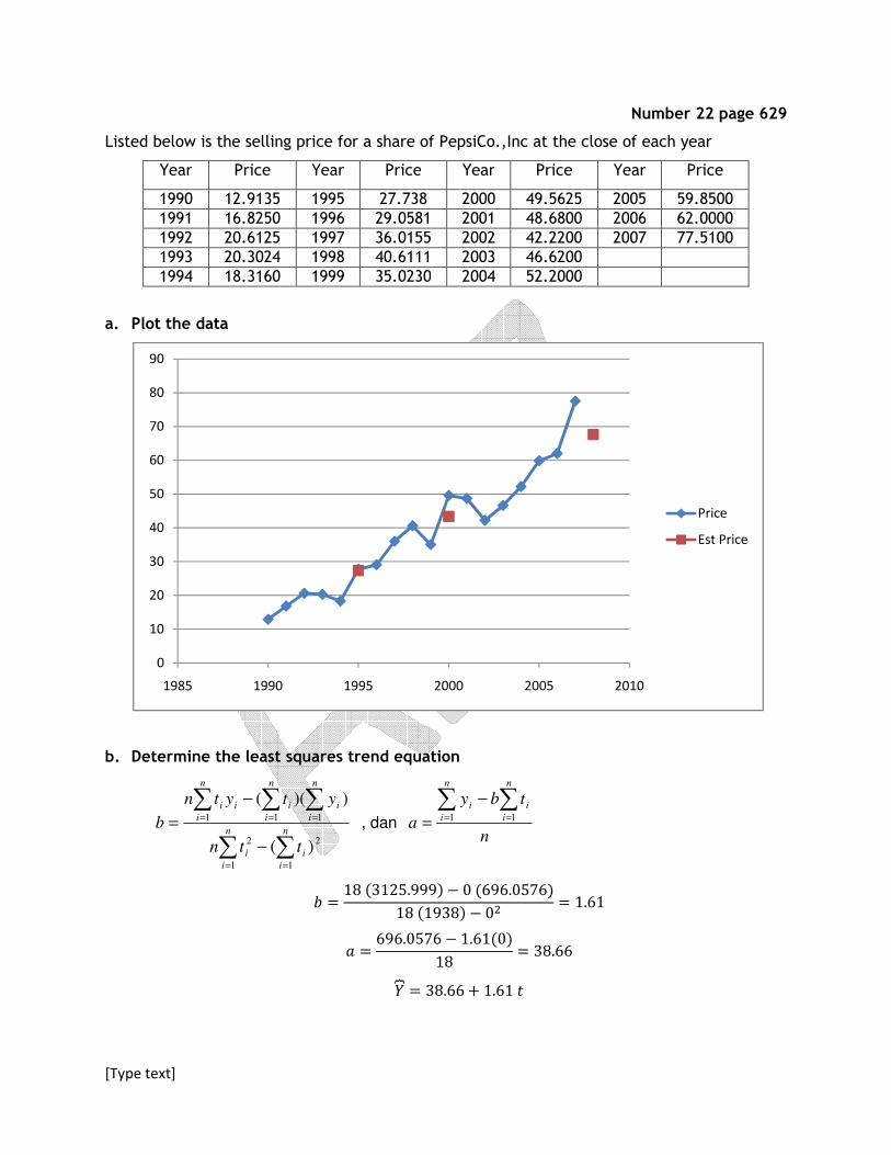
Number 22 page 629

Listed below is the selling price for a share of PepsiCo.,Inc at the close of each year

Year Price Year Price Year Price Year Price

1990 12.9135 1995 27.738 2000 49.5625 2005 59.8500 1991 16.8250 1996 29.0581 2001 48.6800 2006 62.0000 1992 20.6125 1997 36.0155 2002 42.2200 2007 77.5100 1993 20.3024 1998 40.6111 2003 46.6200 1994 18.3160 1999 35.0230 2004 52.2000

a. Plot the data

b. Determine the least squares trend equation

∑∑

∑ ∑ ∑

==

= = =

−

−

=n

i

i

n

i

i

n

i

n

i

n

i

iiii

ttn

ytytn

b

1

2

1

2

1 1 1

)(

))((

, dan n

tby

a

n

i

n

i

ii∑ ∑= =

−

=1 1

� � 18 �3125.999� 0 �696.0576�18 �1938� 0� � 1.61 � � 696.0576 1.61�0�18 � 38.66

�� � 38.66 � 1.61 �

0

10

20

30

40

50

60

70

80

90

1985 1990 1995 2000 2005 2010

Price

Est Price

[Type text]

Tahun Kode (t) Price (Y) KodexProce

(tY) Kode kuadrat (t^2)

1990 -17 12.9135 -219.5295 289 1991 -15 16.825 -252.375 225 1992 -13 20.6125 -267.9625 169 1993 -11 20.3024 -223.3264 121 1994 -9 18.316 -164.844 81 1995 -7 27.738 -194.166 49 1996 -5 29.0581 -145.2905 25 1997 -3 36.0155 -108.0465 9 1998 -1 40.6111 -40.6111 1 1999 1 35.023 35.023 1 2000 3 49.5625 148.6875 9 2001 5 48.68 243.4 25 2002 7 42.22 295.54 49 2003 9 46.62 419.58 81 2004 11 52.2 574.2 121 2005 13 59.85 778.05 169 2006 15 62 930 225 2007 17 77.51 1317.67 289 0 696.0576 3125.999 1938

c. Calculate the points for the years 1995 and 2000

������ � 38.66 + 1.61 (-7) = 27.39 ������ � 38.66 � 1.61 �3� � 43.49

d. Estimate the selling price in 2008

������ � 38.66 � 1.61 �18� � 67.64

[Type text]

e. By how much has the stock price increased or decreased (per year) on average during

the period ? $1.61

Number 23 page 629

If plotted, the following sales series would appear cuvelinear. This indo\icates that sales are

increasing of somewhat constant annual rate (percent) . To fit te sales, therefore, a

logarithmic equation should be used

Year Sales ($million)

Year Sales ($million)

1998 8.0 2004 39.4 1999 10.4 2005 50.5 2000 13.5 2006 65.0 2001 17.6 2007 84.1 2002 22.8 2008 109.1 2003 29.3

a. Determine logarithmic function

� � �� !"# � � !"# � � !"# �

!"# � � $∑ &!"# �& ∑ & ∑ !"#'&$∑ &( �∑ &�(

0

20

40

60

80

100

120

140

160

1994 1996 1998 2000 2002 2004 2006 2008 2010

Sales

Est Sales

[Type text]

!"# � � ∑ !"# �& !"# � ∑ &$

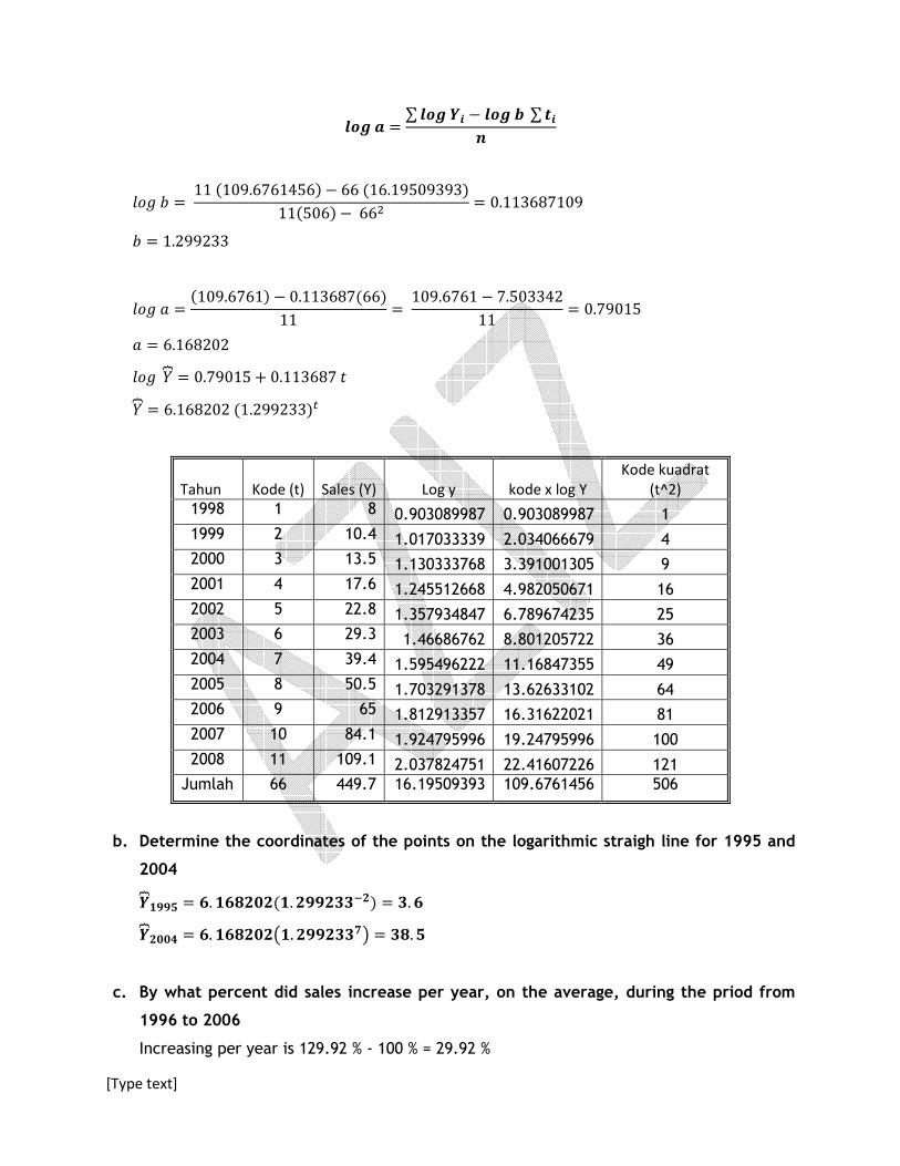
)*+ � � 11 �109.6761456� 66 �16.19509393�11�506� 66� � 0.113687109 � � 1.299233

)*+ � � �109.6761� 0.113687�66�11 � 109.6761 7.50334211 � 0.79015 � � 6.168202 )*+ �� � 0.79015 � 0.113687 � �� � 6.168202 �1.299233�,

Tahun Kode (t) Sales (Y) Log y kode x log Y

Kode kuadrat

(t^2)

1998 1 8 0.903089987 0.903089987 1 1999 2 10.4 1.017033339 2.034066679 4 2000 3 13.5 1.130333768 3.391001305 9 2001 4 17.6 1.245512668 4.982050671 16 2002 5 22.8 1.357934847 6.789674235 25 2003 6 29.3 1.46686762 8.801205722 36 2004 7 39.4 1.595496222 11.16847355 49 2005 8 50.5 1.703291378 13.62633102 64 2006 9 65 1.812913357 16.31622021 81 2007 10 84.1 1.924795996 19.24795996 100 2008 11 109.1 2.037824751 22.41607226 121

Jumlah 66 449.7 16.19509393 109.6761456 506

b. Determine the coordinates of the points on the logarithmic straigh line for 1995 and

2004

��-../ � 0. -01(2(�-. (..(334(� � 3. 0 ��(225 � 0. -01(2(6-. (..(3378 � 31. /

c. By what percent did sales increase per year, on the average, during the priod from

1996 to 2006

Increasing per year is 129.92 % - 100 % = 29.92 %

[Type text]

�����9 � 6.168202�1.299233�� � 65.05 The increasing sales between 1996-2006 (t= 10 years) are 57.04 or average 5.7 % per year

d. Based on the equation, what are the estimated sales for 2009 ?

������ � 6.168202�1.299233��� � 142.7

Number 24 page 629

Reported below are the amount spent on advertising ($million) by a large firm from 1996 to

2006

Year Sales ($million)

Year Sales ($million)

1996 88.1 2002 132.6 1997 94.7 2003 141.9 1998 102.1 2004 150.9 1999 109.8 2005 157.9 2000 118.1 2006 162.6 2001 125.6

0

20

40

60

80

100

120

140

160

180

1994 1996 1998 2000 2002 2004 2006 2008

Adv Expense

Est Adv

[Type text]

a. Determine the logatirmic trend equation

Tahun Kode (t) Sales (Y) Log y kode x log Y

Kode kuadrat

(t^2)

1996 1 88.1 1.944975908 1.944975908 1 1997 2 94.7 1.976349979 3.952699958 4 1998 3 102.1 2.009025742 6.027077226 9 1999 4 109.8 2.04060234 8.16240936 16 2000 5 118.1 2.072249898 10.36124949 25 2001 6 125.6 2.098989639 12.59393784 36 2002 7 132.6 2.122543524 14.85780467 49 2003 8 141.9 2.151982395 17.21585916 64 2004 9 150.9 2.17868924 19.60820316 81 2005 10 157.9 2.19838213 21.9838213 100 2006 11 162.6 2.211120541 24.32232595 121

Jumlah 66 1384.3 23.00491134 141.030364 506

� � �� !"# � � !"# � � !"# �

!"# � � $∑ &!"# �& ∑ & ∑ !"#'&$∑ &( �∑ &�(

!"# � � ∑ !"# �& !"# � ∑ &$

)*+ � � 11 �141.030364� 66 �23.00491134�11�506� 66� � 0.027280873 � � 1.064831458

)*+ � � �23.00491134� 0.02728873�66�11 � � 1.92767034 � � 84.65845527 )*+ �� � 1.92767034 � 0.027280873 � �� � 84.65845527 �1.064831458,�

b. Estimte the advertising expenses for 2009

�� � 84.65845527 �1.064831458.�:� � 203.9870314

[Type text]

c. By what percent per year did advertising expenses during the period?

Average increasing per year = 106.48 % - 100% = 6.48% per year

Number 25 page 629

Listed below is the selling price for a share of aracle,Inc., stock at the close of the year

Year Price Year Price Year Price Year Price

1990 0.1944 1995 3.1389 2000 29.0625 2005 12.2100 1991 0.3580 1996 4.6388 2001 13.8100 2006 19.11 1992 0.7006 1997 3.7188 2002 10.8000 2007 20.23 1993 1.4197 1998 7.1875 2003 13.2300 1994 2.1790 1999 28.0156 2004 13.7200

a. Plot the data

b. Determine the least square trend equation. Use both the actual stock price and the

logarithm of the price.

1. Linier

�� � � � �

∑∑

∑ ∑ ∑

==

= = =

−

−

=n

i

i

n

i

i

n

i

n

i

n

i

iiii

ttn

ytytn

b

1

2

1

2

1 1 1

)(

))((

, dan n

tby

a

n

i

n

i

ii∑ ∑= =

−

=1 1

0

5

10

15

20

25

30

35

1985 1990 1995 2000 2005 2010

Sales

Sales

[Type text]

� � 18�2346.6824� 171 �183.723818�2109� 172� � 1.241

� � 183.7238 1.231�172�18 � 1.583 �� � 1.583 � 1.231 �

Kode (t) Price (Y)

KodexProce

(tY) Kode kuadrat (t^2)

Y

estimate E^2

1 0.1944 0.1944 1

-0.342356 0.28811

2 0.358 0.716 4 0.898731 0.29239 3 0.7006 2.1018 9 2.139817 2.07135 4 1.4197 5.6788 16 3.380903 3.84632 5 2.179 10.895 25 4.62199 5.9682 6 3.1389 18.8334 36 5.863076 7.42113 7 4.6388 32.4716 49 7.104162 6.07801 8 3.7188 29.7504 64 8.345248 21.404 9 7.1875 64.6875 81 9.586335 5.75441 10 28.0156 280.156 100 10.82742 295.434 11 29.0625 319.6875 121 12.06851 288.796 12 13.81 165.72 144 13.30959 0.25041 13 10.8 140.4 169 14.55068 14.0676 14 13.23 185.22 196 15.79177 6.56265 15 13.72 205.8 225 17.03285 10.975 16 12.21 195.36 256 18.27394 36.7714 17 19.11 324.87 289 19.51502 0.16405 18 20.23 364.14 324 20.75611 0.27679 171 183.7238 2346.6824 2109 706.421

;<= � >706.42118 2 � 6.64

[Type text]

2. Curvelinear

� � �� atau !"# � � !"# � � !"# � !"# � � $∑ &!"# �& ∑ & ∑ !"#'&$∑ &( �∑ &�(

!"# � � ∑ !"# �& !"# � ∑ &$

)*+ � � 18 �173.2773255� 171�12.78590356�18�2109� �171�� � 0.106937547 � � 1.279197339

log � � 12.78590356 0.106937547 �171�18 � 0.305578724 � � 0.494790413 log �� � 0.3055 � 0.1069 � atau �� � 0.4948 � 1.2791,�

Tahun Kode

(t) Sales (Y) Log y kode x log Y

Kode

kuadrat

(t^2)

Y

estimate Error

1990 1 0.1944 -0.71130374 -0.71130374 1 0.632935 0.192313

1991 2 0.358 -0.44611697 -0.89223395 4 0.809648 0.203986

1992 3 0.7006 -0.15452987 -0.4635896 9 1.0357 0.112292

1993 4 1.4197 0.152196582 0.608786329 16 1.324865 0.008994

1994 5 2.179 0.33825723 1.691286151 25 1.694763 0.234485

1995 6 3.1389 0.49677748 2.98066488 36 2.167937 0.94277

1996 7 4.6388 0.666405648 4.664839539 49 2.773219 3.480394

1997 8 3.7188 0.570402822 4.563222578 64 3.547494 0.029346

1998 9 7.1875 0.856577858 7.709200719 81 4.537945 7.020143

1999 10 28.0156 1.447399928 14.47399928 100 5.804927 493.314

2000 11 29.0625 1.46333297 16.09666267 121 7.425647 468.1534

2001 12 13.81 1.140193679 13.68232414 144 9.498868 18.58586

2002 13 10.8 1.033423755 13.43450882 169 12.15093 1.825002

2003 14 13.23 1.121559844 15.70183782 196 15.54343 5.351971

2004 15 13.72 1.137354111 17.06031167 225 19.88312 37.98402

2005 16 12.21 1.086715664 17.38745062 256 25.43443 174.8856

2006 17 19.11 1.281260687 21.78143168 289 32.53566 180.2483

2007 18 20.23 1.305995883 23.50792589 324 41.61953 457.5118

171 183.7238 12.78590356 173.2773255 2109 188.421 1850.08

[Type text]

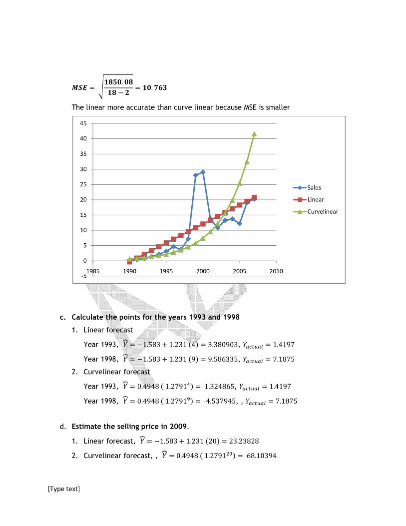
BCD � >-1/2. 21-1 ( � -2. 703 The linear more accurate than curve linear because MSE is smaller

c. Calculate the points for the years 1993 and 1998

1. Linear forecast

Year 1993, �� � 1.583 � 1.231 �4� � 3.380903, �EF,GEH � 1.4197 Year 1998, �� � 1.583 � 1.231 �9� � 9.586335, �EF,GEH � 7.1875

2. Curvelinear forecast

Year 1993, �� � 0.4948 � 1.2791:� � 1.324865, �EF,GEH � 1.4197 Year 1998, �� � 0.4948 � 1.2791�� � 4.537945, , �EF,GEH � 7.1875

d. Estimate the selling price in 2009.

1. Linear forecast, �� � 1.583 � 1.231 �20� � 23.23828 2. Curvelinear forecast, , �� � 0.4948 � 1.2791��� � 68.10394

-5

0

5

10

15

20

25

30

35

40

45

1985 1990 1995 2000 2005 2010

Sales

Linear

Curvelinear

[Type text]

e. By how much has the stock price increases or decreased (per year) on average during

the period?

1. Linear forecast, 23,1 % per year

2. Curvelinear forecast, 27.91 % per year