Institute for Economic Forecasting 10. CASE … · Institute for Economic Forecasting ... A limitation of this paper is that it does not answer the question “what ... county level)

Institute for Economic Forecasting

Romanian Journal of Economic Forecasting –XX (3) 2017 166

DECOMPOSING PRODUCTIVITY

CHANGES – ROMANIA’S COUNTIES CASE 1

Cristina LINCARU2 Speranţa PÎRCIOG3

Abstract The Sectoral Pattern of Growth at county level in Romania may be characterised by “decomposing output growth per worker within sectoral changes and between sectoral changes”. The Job Generation and Growth Decomposition Tool, or JoGGs (Step 3&5) (World Bank, 2011 & Guide), is applied to ten economic sectors (NACE Rev.2) in all 42 counties (NUTS3 level) during the 2010-2013 period. The contribution of each sector, as well as of the inter-sectoral employment shifts, to the observed growth in total output per worker (real 2010 Euros/worker by county) is treated as lattice data (Anselin, 2002). The results are presented in the Chloropleth classification technique univariate maps, by five classes calculated with Jenks natural interval classification scheme. The contribution of each sector to changes in output per worker linked to employment relocation effects offers an image of the manifestation of structural change as a factor behind growth. Keyword: output per worker changes, changes in output per worker within sector,

movements of labour between sectors, structural changes, Locations with sectors with productivity driven by innovation, Locations with sectors without productivity driven by innovation

JEL Classification: O47, O41, O15

1. Introduction In the endeavour to exploit the “new geography of jobs in Romania”, this paper presents some intermediary results. Under Moretti’s (2012) perspective of positive externalities of creative jobs, it provides a spatial labour market analysis. Krugman, Venables and Fujita (1999) explain in the New Economic Geography how production is heterogeneously distributed over space, reflecting the agglomeration tendency 1 This paper was presented in the Section IV - Economic Development, Innovation, Growth from

the 3rd International Conference: Recent Advances in Economic and Social Research May 11-12, 2017, Institute for Economic Forecasting, Romania;

2 National Scientific Research Institute for Labor and Social Protection – INCSMPS, E-mail: [email protected]

3 National Scientific Research Institute for Labor and Social Protection – INCSMPS, E-mail: [email protected]

10.

Decomposing productivity changes – Romania’s counties case

Romanian Journal of Economic Forecasting – XX (3) 2017 167

in highly populated locations (countries, regions, and localities), but also the trend of increasing income in the same areas of success. Ernst & Berg (2009, p.41) point out that employment is essential in “achieving growth with equity”. Komlos (2016, p. 513) makes a new insight regarding the need to re-evaluate the importance of concentration and power (source of monopoly/oligopoly) from the perspective of perfect markets, considering that “any concentration of power is a threat to freedom”. Also, in the recent “Creative destruction” essay, Komlos (2017) proves that innovation is one important source of inequality, in both agglomeration formation and distribution mechanisms. Komlos’s analysis is made on the background that the “contribution of the innovation to employment will be small and its impact on GDP growth will likely be modest and overestimated insofar as the accounts fail to account accurately for the negative externalities caused by the destructive forces of creative destruction” (Komlos, 2017). In this context, he warns that “creative destruction has become more destructive recently about its creative component”. Moretti (2012) proves that some spatial agglomeration allows high return rates of investments (capital) if there is a high concentration of creative people. These locations have spillover effects and positive externalities with diminishing labour market dysfunctionalities at local and regional levels. Pelinescu (2015, p. 189) highlighted “the importance of human capital in ensuring economic growth expressed as gross domestic product per capita”. An externality is a large indirect effect of “consumption, production, and investment decisions of individuals, households, and firms [that] often affect[s] people not directly involved in the transactions” (Helbling, 2012). If the affected party is "fully compensated by the others for this effect then the market has failed and government intervention is potentially justified”. Broadening the framework of economic activities from the sustainability perspective demands that, beyond the direct transaction from production and consumption processes, it also includes both the positive and the negative externalities of promoting eco-innovation (Rennings, 1998 and 2000). Eco-innovation opens new opportunities, mixing creation and destruction processes. (OECD, 2011; OECD, 2012). The analysis of sectoral structure changes in employment and economic growth at the regional level was made by Jula et al. (2013, p. 52), by expanding the Dobrescu model (2011). Jula et al. found “that growth causes structural changes in total regional employment and for regional activities in manufacturing, real estate activities, wholesale and retail, education, mining and quarrying, financial intermediation and insurance, health and social assistance, administrative services, and construction”, but they “reject the hypothesis that structural changes in regional employment cause regional GDP to grow”. Pelinescu et al. (2015c, p.10) look at regional competitiveness as the “aggregate competitiveness of firms and derivative of macroeconomic competitiveness”. The profile of economic growth and competitiveness at county level is complemented with external competitiveness patterns. The partial breakdown of the productivity growth profile has as its main objectives: How is growth reflected in the changes in output per worker? (World Bank, 2011, p. 7) How is growth reflected in the sectoral pattern of growth? (World Bank, p.7). This work is a follow-up to Lincaru (2015, 2016) and Lincaru & Pirciog (2017). A limitation of this paper is that it does not answer the question “what are the sources of changes in output per worker”. The World Bank methodology considers three different sources: i) increases in the capital-labour ratio; ii) increases in Total Factor Productivity (TFP); and iii) relocation of jobs between bad jobs sectors (low productivity) to good job sectors (high productivity). The relocation of jobs is described as a component of growth in output per worker, or as the labour reallocation effect (World Bank, p. 23). Regarding sector



boundaries, we analyse the changes in output per worker within the sector and outside the sector, combing steps 3 and 5 of the World Bank methodology. Regardless of the sources of change in total output per worker (net of inter-sectoral shifts) at the aggregate level, we consider that productivity growth is induced by innovation in both dimensions of capital and knowledge, or “productivity-enhancing innovation” Gordon (2016, cited from Komlos 2017). As a consequence, following Komlos (2016), we consider that the substitution effect of innovation is a negative labour reallocation effect and that the positive externality is employment growth in the sector with productivity growth. The value (significance) of the study is considered as a better understanding of labour market functioning, on the background of spatial heterogeneity of economic growth (at the county level). This paper is anchored in the framework of endogenous growth theory and sheds light on some essential characteristics of human capital (skills, knowledge value or people – Pelinescu, 2015, p.184), social capital, intangible actives (Pelinescu et al., 2015b, p. 8) and labour market functioning (intra- and inter-sectoral labour force reallocation, but not taking into consideration skills matching quality). The main reason to apply this model is to exploit better sample data, which are easily accessible by providing a monitoring process of labour market functioning, tracking valuable inputs in education and skill formation, and improving its functioning framework (as it is the employment protection legislation, EPL) (OECD, 2007, p. 13).

2. Data The aim of JoGGs World Bank methodology is “to understand how growth is linked to changes in employment, output per worker and population structure at the aggregate level and by sectors” (World Bank, 2011, p.4), (Ajakaiye, 2015). The Romanian counties’ growth profile for the 2010-2013 period, given by the changes in aggregate output per worker, is based on Steps 3 and 5 of the JoGGs. Step 3 focuses on decomposing output growth per worker within sectoral changes and between sectoral changes, and Step 5 focuses on the “understanding of the role of inter-sectoral employment shifts”. The “Decomposition Tool – JoGGs” is applied for the first time in Romania to ten economic sectors (NACE Rev.2) in all 42 counties (NUTS3 level) during the 2010-2013 period. The contribution of each sector, as well as of inter-sectoral employment shifts, to the observed growth in total output per worker (real 2010 Euros/worker by county) are treated as lattice data (Anselin, 2002). The results are presented in the Chloropleth classification technique univariate maps, made in Arc GIS Desktop, by five classes calculated with Jenks natural interval classification scheme. The JoGGs county results are treated as spatially vectorised variables using Arc GIS 9.3. In this approach, the counties have both dimensions: geographical and administrative as well as attribute data - the socio-economic indicators used in JoGGs (input, output and the result ones). The geographical dimension is also an administrative dimension. The ESRI 2014 generated polygons used in spatial vectorising of the data are the administrative boundaries described by SIRUTA – Information System of the Register of the Territorial-Administrative Units managed by the National Institute of Statistics (NIS). The county level is codified at level 1 in (SIRUTA), which is equivalent to level 3 in the EU NUTS framework. The county is the main territorial-administrative unit, which is both organisationally and functionally relevant in the socio-economic and statistical systems, as it is a multidimensional integrator. By law, the “county is an administrative-territorial unit composed of municipalities, towns, and communes as the core unit of administrative-territorial organisation of the country,



conditional on the geographical, economic and social-political, ethnic, cultural and traditional ties to the population.” The socio-economic dimension represented by the attribute data is linked in space. Attribute data are structured with reference to the JoGGs model as input level characteristics, intensity level characteristics, data and output data resulting from the model. Y - Gross Value Added (GVA): source Eurostat [nama_10r_3gva], deflated at 2010 real

prices. Y is used by 10 NACE Rev 2. sectors in 2010 (Y2010) and 2013 (Y2013) and rY1013 is the growth rate of GVA (%) during the 2010-2013 period;

N - Total population: National Institute of Statistics (NIS) TEMPO data (POP107A - Population by Domicile on 1 January), the total population for 2010 and 2013 (N2010, N2013) and rN1013 is the growth rate during the 2010-2013 period;

A - The working age population: NIS TEMPO data (FOM101A – Work Resources), the total working age population 15-64 years old in 2010 and 2013 (A2010, A2013) and rA1013 is the growth rate during the 2010-2013 period;

E - The employed population: NIS TEMPO data (FOM103D - employed civilian population), employment for 2010 and 2013 (E2010, E2013) and rE1013 is employment growth rate (%) during the 2010-2013 period;

Four input intensity characteristics : Y/N = y, GVA/capita as a proxy for income per capita, calculated for 2010 and 2013

(Y/N2010, Y/N2013) and rY/N1013 is the growth rate of income per capita (%) during the 2010-2013 period;

Y/E=ω, productivity as output per worker (GVA/worker), calculated for 2010 and 2013 (Y/E2010, Y/E 2013) and rY/E1013 is the growth rate of productivity (%) during the 2010-2013 period;

E/A = e, employment rate, calculated for 2010 and 2013 (E/A2010, E/A 2013) and rE/A1013 is the growth rate of employment (%) during the 2010-2013 period;

A/N=a, the share of the labour force in total population as the activity rate, calculated for 2010 and 2013 (A/N2010, A/N2013, and rA/N1013) is the growth rate of active population (%) during the 2010-2013 period.

3. Model The spatial analysis was conducted with the "Choropleth map" technique by the classification scheme with "Jenks” natural intervals of Arc Gis software 10.2.3. The ESDA Choropleth maps with polychrome progression fall within the broad family of Exploratory Spatial Data Analysis. The Choropleth maps are next to percentile, boxing, cartogram, and hinge basic tools that provide a synthetic image by data geo-visualization. (Anselin, 2005, p.78). This classification scheme is manually applied to five classes (minimum number of classes, impact to provide a central class). The map attributes input data are the results of the JoGGs model for each county. These results are per capita normalised per county, equivalent to rate smoothing. Natural breaks (Jenks) is an optimised classification scheme, with five intervals manually established using an iterative procedure that divides values into classes that minimises within-group variability and maximises between-group variability, in an attempt to create the most homogenous classes that are possible with the dataset (Slocum et al., 2009). The result of this method is the visualisation of spatially vectorized statistical quantitative socio-economic information. Thus, considering all constraints and advertising forms theory, the maps are comparable.



The output per worker breakdown into changes in output per worker within sectors and movements of labour between sectors

In Step 3 of the JoGGs methodology using the Shapley approach, the changes in aggregate output per worker can be decomposed into changes in output per worker within sectors (also known as the “within” component) and movements of labour between sectors (also referred to as the “between” component). (JoGGs, p.19).

= ∑ (1)where: Yij = total Gross Added Value; j = County, from 1 to 42; i = sector of economic activity from 1 to 10; Ei - employment in sector i. Equation (1) basically denotes that the “output per worker is the weighted sum of output per worker in all sectors, where the weights are simply the employment shares of each sector” (JoGGs, p.19, detailed at p.39):

= ∑ (2)where: Y/E=ω output per worker or the total productivity; s=Ei/E the share of sector i in total employment. The logic of this approach is based on the “intuition” that “increases in output per worker within a sector will increase the average output per worker. How large the effect is will depend on the size of each sector (i.e., its share in total employment). On the other hand, the relocation of workers across sectors of different productivity levels can increase the average output per worker if the final relocation implies that a larger share of workers becomes employed in higher productivity sectors.” (JoGGs, p.19). Δωj=ΔωBj+Δωwj (3)Where applying Shapley approach :

Δω - changes in aggregate output per worker or productivity; (real prices, 2010 Euro/worker); ∆ωB - the change in output per worker due to inter-sectoral employment changes (i.e. net movements of workers between sectors); (real prices, 2010 Euro/worker); ∆ωw - the change in output per worker due to changes in output per worker in sector i; it corresponds to total changes in output per worker net of relocation effects, which is also referred to as the ‘within component’ (real 2010 prices, Euro/worker).

Considering that "once we can trace the growth in output per worker back to its within and between components, we can then calculate the amount of growth in total output per capita that can be linked to changes in output per worker in sector i, and to inter-sectoral relocation of labor by combining the contribution of each of these components to changes in output per worker with the contribution of changes in output per worker to total per capita growth (obtained in step 1). As before, the contribution of changes in output per worker within a sector can be interpreted as the total per capita growth consistent with a counterfactual scenario, in which all the others (employment rate, demographics, and output per worker in the remaining sectors) remained unchanged and the only change was the observed change in output per worker in sector i. The contribution of the intersectoral shift component can be interpreted as a counterfactual scenario in which the employment rate, the demographic structure of the population and output per worker in each sector remained unchanged, and labour reallocated across sectors as observed.” (World Bank JoGGs, p.19)



Estimating the role of inter-sectoral employment shift

Step 5 of the JoGGs methodology analyses the role of inter-sectoral employment shifts. The productivity breakdown into within and between sectors is linked with the magnitude of employment shifts between sectors, offering an image of the structural change linked with productivity positive and negative externalities: this is “an important factor behind growth.” (World Bank JoGGs p.42) The structural change is the “movement of labour force shares from low productivity sectors to high productivity sectors” (World Bank JoGGs p.42), where “changes in the share of employment in the different sectors help to explain the overall contribution of inter-sectoral shifts to output per worker”. The JoGGs methodology uses the following interpretation: “Thus if sector i has productivity below the average productivity and increases its share, si, its contribution will be positive; that is, outflows from this low productivity sector have contributed to the increase in output per worker. If, on the other hand, the sector reveals an increase in its share, the inflows into this low productivity sector will decrease output per worker and, thus, will have a negative effect on the inter-sectoral shift term” (World Bank JoGGs p.42). In the context of reference to productivity driven by innovation and its externalities (positive or negative over the employment), we propose the following “understanding” of the results: In sectors with positive externalities of worker outflows on productivity that have contributed to the increase in output per worker:

If there is a positive change in the share of employment in sectors with higher productivity than the average (at county level), there are increasing inflows in sectors with higher productivity levels. In this situation, there is a visible and positive externality on the labour force (the Moretti case). Also, this case indicates the presence of productivity driven by innovation, with positive externalities in the sector;

If there are negative changes in the share of employment in sectors with productivity lower than the average productivity (here at county level), there are increasing outflows from sectors with lower productivity levels (the substitution effect – Komlos). Also, this case indicates the presence of productivity driven by innovation, with negative externalities in the sector.

In sectors with negative externalities of workers flow on productivity that has contributed to the decrease in output per worker:

If there is a positive change in the share of employment in sectors with productivity lower than average (at county level), there are increasing inflows in sectors with lower productivity levels. In this situation, there is a visible and positive externality on the labour force, but it is not sustainable. This case indicates the absence of productivity driven by innovation in the sector.

If there are negative changes in the share of employment with productivity higher than average (at county level), there are increasing outflows from sectors with higher productivity levels. Here, the substitution effect is present (Komlos). Also, this case indicates the presence of productivity driven by innovation, with negative externalities in the sector.



4. Results4 The productivity breakdown into within and between sectors components is linked to the magnitude of employment shift between sectors at county level, and offers some homogenous and other heterogeneous aspects that are relevant for the good functioning of the labour market. Homogenous aspects are visible in the input data in 2013 for the A, R-U, G-I and O-Q sectors. Agriculture (A) with all the counties, Professionals and Arts (R-U) with 41 counties, Commerce (G-I) with 38 counties, and Public Administration (O-Q) with 34 counties are the sectors with average levels of productivity below the national average of 13.94 thousand 2010 Euros/worker, real prices. These sectors are eligible for productivity enhancement applied at national scale. Changes in aggregate output per worker, or the changes in total productivity, were spatially heterogeneous during the 2010-2013 period. We registered positive changes in aggregate output per worker in 26 counties and negative changes in 16 counties. The highest positive productivity changes were in Constanta and Prahova, with values above 3460 Euros/worker, 2010 real prices, followed by Ilfov, Cluj and Bucharest, with important positive levels of changes in aggregate productivity (over 1000 real 2010 Euros/worker). The highest negative changes of productivity were registered in Arges and Giurgiu counties, which experienced levels below -1645 Euros/worker, 2010 real prices. The counties clustered into a regional development pattern by North-East, East, and North, and Bucharest-Ilfov recorded productivity gains, while the counties in the West and Central regions experienced a decrease. The aggregate within-sector productivity changes registered positive values in 20 counties and negative values in 22 counties (Figure 11). The highest negative aggregate within-sector productivity changes were registered in Giurgiu, Argeș, Alba, Mehedinți, Călărași and Bacău, with a level below -1000 real 2010 Euros/worker. The highest positive aggregate within-sector productivity changes were registered in Constanta, Prahova, Ilfov, Tulcea, Buzau, Bucuresti and Vaslui, with a level over 1100 real 2010 Euros/worker. The within-sector productivity changes (see Annex 1) by sector contribution were:

Independent by space - with low variations across counties in: - The sectors O-Q and R-U do not register variations of the within productivity changes. The minimum level was relatively close to the maximum level (- 92 real 2010 Euros/worker; 152 real 2010 Euros/worker) (Figure 9 and Figure 10);

Dependent on space a. With relatively low variance

- The F and J sectors registered the same tendency of decreasing within-productivity changes. The minimum level was relatively high (negative), and the maximum level was very low (- 1392 real 2010 Euros/worker; 136 real 2010 Euros/worker) (Figure 3 and Figure 5); - The K, M-N and A sectors saw the same tendency of increasind within-productivity changes. The minimum level was relatively low (negative), and the maximum level was high (-236 real 2010 Euros/worker; 1529 real 2010 Euros/worker) (Figure 6, Figure 8 and Figure 1);

4 All figures are available as Supplementary Annex on http://www.rjef.ro.



b. With relatively high variance - The B-E, and L and G-I sectors showed the tendency of varying within-productivity changes. They revealed high amplitude, as both the minimum and the maximum levels were high (-2244 real 2010 Euros/worker; 2577 real 2010 Euros/worker) (Figure 2, Figure 7 and Figure 4). This result could be explained by looking at the “Guevara-Rosero conclusion” (2017, p.75), which states that the effect of trade on the spatial concentration of a population depends upon the characteristics of regions” (i.e., depends on the dimensions of the home market, location advantages, the degree of access to international trade, historical disadvantages, etc.) This approach needs to be revisited in a future study.

The aggregate between-sectors productivity changes registered positive values in 32 counties and negative values in 10 counties (Figure 11). The highest negative aggregate between-sector productivity changes were registered in Tulcea and Bistrita-Nasăud, with a level below -1000 real 2010 Euros/worker. The highest positive aggregate between-sector productivity changes were registered in Călărași, Alba and Mehedinți, with a level over 1100 real 2010 Euros/worker. The between-sector productivity changes (see Annex 1) by sector contribution were:

Independent of space - with low variations across counties in: - The K, R-U, O-Q, G-I, F, B-E and M-N sectors, which did not register important variations in the between-sectors productivity changes. The minimum level was relatively close to the maximum level (- 117 real 2010 Euros/worker; 138 real 2010 Euros/worker) (Figure 6, Figure 10, Figure 9, Figure 4, Figure 3, Figure 2 and Figure 8);

c. Dependent on space – with relatively high variance in: - The A and J sectors, with the tendency of increasing between-sectors productivity changes. The minimum level was relatively low (negative), and the maximum level was high (-43 real 2010 Euros/worker; 720 real 2010 Euros/worker) (Figure 1 and Figure 5); - The L sector, with the tendency of variation of between-sectors productivity changes. It has revealed high amplitude, both the minimum and the maximum levelsweare high (-1119 real 2010 Euros/worker; 1356 real 2010 Euros/worker) (Figure 7);

Looking at the average values for the period 2010-2013, the changes in aggregate output per worker (Δω) are mostly explained by the change in output per worker due to sectoral changes (∆ωw). The linear regression model indicates that if the output per worker in the sector increases by 1 Euro per worker (in 2010 real prices), then the aggregate output per worker increases by 0.819 real 2010 Euros per worker. Also, the coefficient of determination is high, indicating that 83% of the variability between the two variables is accounted for. The changes in aggregate output per worker have no relation with the net movements of workers between sectors (∆ωB). If ∆ωB increases, there is a visible tendency of decreasing changes in total productivity. This general result is consistent with Isaksson’s finding that for countries with economies in transition, “the within effect dominates, but as expected, its contribution is smaller than that in industrialised countries” (Isaksson, 2010, p.9). Pushed by technological progress, change, and knowledge, a sector needs to use and exploit specific skills. It should invest in training and new skills creation as a source of increasing human capital and, implicitly, increasing productivity within the sector. This process is dynamic and continuous. Next, the main process of increasing the within-sector



productivity demands adjusting for the optimum balance of demand through the movement of labour force between sectors. Locations with sectors with productivity driven by innovation Sectors with positive externalities of worker outflows on productivity that have contributed to the increase in output per worker:

With the positive change in the share of employment in sectors with productivity higher than average, increasing inflows in sectors with higher productivity levels will have positive externalities on the labour force, indicating the presence of productivity driven by innovation, with positive externalities in the sector:

- In the M-N sectors in 34 counties (Alba, Arad, Arges, Bacau, Bihor, Botosani, Braila, Buzau, Calarasi, Caras-Severin, Cluj, Dâmbovita, Dolj, Galati, Giurgiu, Harghita, Hunedoara, Ialomita, Iasi, Ilfov, Mehedinti, Mures, Neamt Olt, Prahova, Sibiu, Suceava, Teleorman, Timis, Tulcea, Vaslui, Vrancea, Salaj, Bucuresti; see Figure 8); - In the J sector in 9 counties (Bihor, Cluj, Dâmbovita, Sibiu, Suceava, Teleorman, Vaslui, Vrancea, Satu Mare; see Figure 5); - In the L sector in 9 counties (Bacau, Braila, Caras-Severin, Dâmbovita, Iasi, Neamt, Prahova, Timis, Constanta; see Figure 7); - In the B-E sectors in 7 counties (Bistrita-Nasaud, Brasov, Buzau, Calarasi, Prahova, Suceava, Satu-Mare; see Figure 2); - In the R-U sectors in 3 counties (Giurgiu, Ilfov, Salaj; see Figure 10); - In the F sector in one county, Galati; see Figure 3; - In the G-I sectors in one county, Neamt; see Figure 4; - In the K sector in one county, Ilfov; see Figure 6.

This model (1,1,1,1)5 is characterised by the sectoral level of average productivity over the average productivity level of the county. It presents a tendency for positive structural changes, in the sense of increasing the contribution of the sector in the GVA of the economy. This process is based on increasing productivity and the share of employment in the sector, while labour force reallocation within the sector is observed from the lower productivity towards higher productivity jobs, a process accompanied by positive income change. In this case, the productivity is innovation-driven and is accompanied by at least two positive externalities: job creation and increase in income. This structural change is positive and sustainable.

In sectors6 with productivity that is lower than the average, increasing within-sector productivity with positive change in the share of employment increasing inflows in sectors with higher productivity level will have positive externalities on labour force via

5 Digit (Tw01) – 1 if the productivity of the sector is higher than the average productivity of the

county, else 0; Digit 2 (dww) – 1 if the within productivity of the sector is increasing, else 0; Digit 3 (dwB) – 1 if the positive reallocation of the labour force from lower productivity sectors toward higher productivity sectors also indicates the presence of positive income externalities; Digit 4 (AdsiB) - 1 if positive structural change given by increasing the share of employment in the sector tendency

6 . TAw01 dww dwB dsiB

0 1 0 1



job creation, indicating the presence of productivity driven by innovation, with partial positive externalities in the sector. Meanwhile, income is not increasing:

- in the G-I sectors in 32 counties (Arad, Arges, Bacau, Botosani, Braila, Buzau, Cluj, Covasna, Dâmbovita, Dolj, Galati, Harghita, Hunedoara, Ialomita, Iasi, Ilfov, Mehedinti, Mures, Olt, Prahova, Sibiu, Suceava, Timis, Tulcea, Vâlcea, Vaslui, Vrancea, Salaj, Satu Mare, Bucuresti, Constanta, Maramures; see Figure 4); - in the M-N sectors in 3 counties (Brasov, Gorj, Constanta; see Figure 8); - in the A sector in 2 counties (Braila, Bucuresti; see Figure 1); - in the R-U sectors in one county (Hunedoara; see Figure 10);

Negative changes in the share of employment and productivity lower than the average and increasing outflows from sectors with lower productivity levels indicate the presence of productivity driven by innovation, with negative externalities in the sector:

- In the A sector in 30 counties (Alba, Arad, Arges, Bacau, Bihor, Botosani, Brasov, Buzau, Calarasi, Covasna, Dâmbovita, Dolj, Giurgiu, Gorj, Hunedoara, Ialomita, Iasi, Ilfov, Neamt, Olt, Prahova, Sibiu, Suceava, Teleorman, Tulcea, Vâlcea, Vaslui, Vrancea, Salaj, Satu Mare; see Figure 1).; - In G-I sectors in one county, Brasov; see Figure 4; - In O-Q sectors in 5 counties (Arad, Brasov, Cluj, Timis, Constanta; see Figure 9);

This model (0,1,1,0) is characterised by a level of average productivity in the sector below the average productivity level of the county. It reveals a tendency toward positive structural change, in the sense of releasing the labour force (decreasing the employment share of the sector in total employment) and reallocating labour towards sectors with higher productivity and, thus, with higher income. The positive structural change reflects a positive externality effect on income. Locations with sectors without productivity-driven by innovation: Sectors with negative externalities of worker productivity flows that have contributed to the decrease in output per worker:

Sectors7 with productivity higher than the county average have a positive change in the share of employment in the sector and increasing inflows in sectors accompanied by increasing income but are not correlated with increasing productivity. This process has the effect of decreasing the within-productivity of the sector. This case, on the background of a decreasing within-sector productivity level, indicates the absence of productivity driven by innovation in the sector:

- in the J sector in 23 counties (Arad, Arges, Bacau, Bistrita-Nasaud, Botosani, Braila, Brasov, Buzau, Calarasi, Caras-Severin, Covasna, Dolj, Galati, Ialomita, Iasi, Ilfov, Mures, Neamt, Tulcea, Vâlcea, Salaj, Bucuresti, Maramures; see Figure 5); - in the F sector in 22 counties (Alba, Bacau, Bihor, Bistrita-Nasaud, Botosani, Braila, Buzau, Calarasi, Covasna, Giurgiu, Harghita, Hunedoara, Ialomita, Mehedinti, Neamt, Suceava, Teleorman, Vaslui, Vrancea, Salaj, Satu Mare, Maramures; see Figure 3); - in the R-U sectors in 19 counties (Bacau, Bihor, Botosani, Buzau, Calarasi, Covasna, Dâmbovita, Dolj, Galati, Harghita, Iasi, Mehedinti, Mures, Olt, Vâlcea, Vaslui, Vrancea, Satu Mare, Maramures; see Figure 10);

7 TAw01 dww dwB dsiB

1 0 1 1



- in the L sector in 18 counties (Alba, Botosani, Brasov, Calarasi, Cluj, Dolj, Galati, Gorj, Harghita, Hunedoara, Mehedinti, Mures, Olt, Sibiu, Suceava, Teleorman, Vrancea, Maramures; see Figure 7); - in the B-E sectors in 15 counties (Alba, Arad, Arges, Bihor, Botosani, Dolj, Giurgiu, Neamt, Olt, Sibiu, Teleorman, Timis, Vrancea, Salaj, Maramures; see Figure 2); - in the G-I sectors in 5 counties (Calarasi, Caras-Severin, Giurgiu, Gorj, Teleorman; see Figure 4); - in the M-N sectors in 3 counties (Bistrita-Nasaud, Satu Mare, Maramures; see Figure 8);

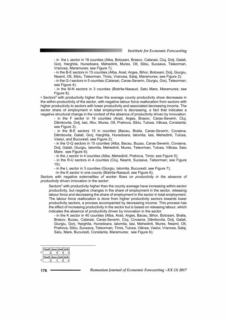
• Sectors8 with productivity higher than the average county productivity show decreases in the within-productivity of the sector, with negative labour force reallocation from sectors with higher productivity to sectors with lower productivity and associated decreasing income. The sector share of employment in total employment is decreasing, a fact that indicates a negative structural change in the context of the absence of productivity driven by innovation.

- in the F sector in 16 counties (Arad, Arges, Brasov, Caras-Severin, Cluj, Dâmbovita, Dolj, Iasi, Ilfov, Mures, Olt, Prahova, Sibiu, Tulcea, Vâlcea, Constanta; see Figure 3); - in the B-E sectors 15 in counties (Bacau, Braila, Caras-Severin, Covasna, Dâmbovita, Galati, Gorj, Harghita, Hunedoara, Ialomita, Iasi, Mehedinti, Tulcea, Vaslui, and Bucuresti; see Figure 2); - in the O-Q sectors in 15 counties (Alba, Bacau, Buzau, Caras-Severin, Covasna, Dolj, Galati, Giurgiu, Ialomita, Mehedinti, Mures, Teleorman, Tulcea, Vâlcea, Satu Mare; see Figure 9); - in the J sector in 4 counties (Alba, Mehedinti, Prahova, Timis; see Figure 5); - in the R-U sectors in 4 counties (Cluj, Neamt, Suceava, Teleorman; see Figure 10); - in the L sector in 3 counties (Giurgiu, Ialomita, Bucuresti; see Figure 7); -in the K sector in one county (Bistrita-Nasaud; see Figure 6);

Sectors with negative externalities of worker flows on productivity in the absence of productivity driven innovation in the sector:

Sectors9 with productivity higher than the county average have increasing within-sector productivity, but negative changes in the share of employment in the sector, releasing labour force and decreasing the share of employment in the sector in total employment. The labour force reallocation is done from higher productivity sectors towards lower productivity sectors, a process accompanied by decreasing income. This process has the effect of increasing productivity in the sector but is based on releasing labour, which indicates the absence of productivity driven by innovation in the sector.

- in the K sector in 40 counties (Alba, Arad, Arges, Bacau, Bihor, Botosani, Braila, Brasov, Buzau, Calarasi, Caras-Severin, Cluj, Covasna, Dâmbovita, Dolj, Galati, Giurgiu, Gorj, Harghita, Hunedoara, Ialomita, Iasi, Mehedinti, Mures, Neamt, Olt, Prahova, Sibiu, Suceava, Teleorman, Timis, Tulcea, Vâlcea, Vaslui, Vrancea, Salaj, Satu, Mare, Bucuresti, Constanta, Maramures; see Figure 6);

8 .

9

TAw01 dww dwB dsiB1 0 0 0




- in the O-Q sectors, in 16 counties (Bihor, Bistrita-Nasaud, Botosani, Braila, Calarasi, Dâmbovita, Harghita, Hunedoara, Iasi, Neamt, Olt, Suceava, Vaslui, Vrancea, Salaj, Maramures; see Figure 9); -in the L sector in 12 counties (Arad, Arges, Bihor, Bistrita-Nasaud, Buzau, Covasna, Ilfov, Tulcea, Vâlcea, Vaslui, Salaj, Satu Mare; see Figure 7); - in the B-E sectors in 5 counties (Cluj, Ilfov, Mures, Vâlcea, Constanta; see Figure 2); - in the J sector in 4 counties (Giurgiu, Harghita, Hunedoara, Olt; see Figure 5); - in the M-N sectors in 2 counties (Covasna, Vâlcea; see Figure 8); - in the R-U sectors in one county (Bistrita-Nasaud; see Figure 10);

Sectors10 that have productivity lower than the county average show decreasing within-sector productivity with positive changes in the share of employment in the sector. Labour force inflows increase the share of employment in the sector in total employment. The labour force reallocation is done from lower productivity sectors towards lower productivity sectors, a process accompanied by decreasing income. This process has the effect of decreasing productivity in the sector and is accentuated by increasing labour inputs, indicating again the absence of productivity driven by innovation in the sector

- in the G-I sectors, in 3 counties (Alba, Bihor, Bistrita-Nasaud; see Figure 4); - in the A sector, in one county (Caras-Severin; see Figure 4); - in F and J sectors in Gorj county; see Figures 3 and 5)

Sectors11 that have productivity lower than the county average show decreasing within-sector productivity and negative changes in the share of employment in the sector. The share of employment in the sector is decreasing in terms of total employment. The labour force reallocation is done from low productivity sectors towards lower productivity sectors, but the process is accompanied by increasing income. This process has the effect of decreasing productivity in the sector and is accompanied by releasing labour and increasing income, indicating the absence of productivity driven by innovation in the sector.

- In the A sector, in 9 counties (Bistrita-Nasaud, Cluj, Galati, Harghita, Mehedinti, Mures, Timis, Constanta, Maramures; see Figure 1); - In the O-Q sectors, in 6 counties (Arges, Gorj, Ilfov, Prahova, Sibiu, Bucuresti; see Figure 9); - In the R-U sectors, in 4 counties (Arad, Brasov, Ialomita, Bucuresti; see Figure 10); - In the F sector, in 2 counties (Timis, Bucuresti; see Figure 3);

5. Discussion Aghion et al. (2009, p.12) select four growth paradigms: the Neoclassical Growth Model, the AK Model, the Product-Variety Model and the Schumpeterian Model (creative destruction). Growth accounting was measured under the standard neo-classical equilibrium concept. The evolutionary economists (e.g., Dosi, 1988; Nelson and Winter, 1982; Nelson, 1981) point out that “equilibrium concepts may be the wrong tools to approach the measurement of productivity change, because if there truly were equilibrium, there would be no incentive

10

11 .





to search, research and innovate, and there would be no productivity growth” (OECD, p. 120). Griliches (1997) links productivity growth with investment in human capital, noting that “accounting is not explaining the underlying causes of growth”. Nelson and Winter (1974) consider the Schumpeterian alternative to neoclassical theory, specifically with the elements of evolutionary growth theory. The limits of this model are many, as it treats sectors equally regardless of their type (OECD, 2001); considers a closed system as its unit of analysis (county); and excludes entry/exit to/from the system (labour market entry for young people in their first job, exits from the national labour market through retirement or external migration/mobility for work). Another limit is the absence of productivity sources (TFP and capital investment) as a profile subject of Step 5 of the JoGGs analysis. The link between productivity and innovation is indirect (based on logic exclusion), with reference to within- and between-sector labour force reallocation, but without regard for the level of scope (local, regional, national, global, etc.). • The paper contributes to the literature by changing the logical criteria to whether or not productivity is driven by innovation (0 or 1, yes or no) at the county level. When the presence of innovation is indirectly identified, some positive or negative socio-economic externalities may be noticed. Also, this approach is more speculative regarding productivity breakdown and its link to the presence of innovation. The JoGGs methodology is relatively simple, with available data: it is an instrument that is capable of monitoring the growth profile. It is composed of issues characterising the “quality of innovation” from the presence of externalities (here, only social – employment/job creation, income level, reallocation effects, structural changes). The within-sector productivity dynamics is linked to the within- and between-sectors labour force reallocation, with direct implications on the share of sector employment in total employment as a reflection of structural change. This logic is integrative, also considering the level of productivity with reference to the average productivity of the county. If the full puzzle of the JoGGs methodology is put together, the growth profile links with the quality of life output. • The spatial scale of analysis is relevant to the sector type. - The aggregate within-sector productivity changes are space independent in O-Q and R-U sectors and highly space dependent in the B-E, l and G-I sectors. Within-sector productivity could be managed by policies at national level for independent sectors, and regional policies could be developed for spatially dependent sectors. - The aggregate between-sector productivity changes are space independent in the K, R-U, O-Q, G-I, F, B-E and M-N sectors and space dependent for the J and L sectors. The ease of labour force reallocation independent of space reflects occupational mobility, on one side, with reflected high specialisation, on the other side. Identifying locations at NUTS level 3 is only part of the broader analysis initiated in this study. More accurate locations and active economic activities are positive externalities to be explored by modelling microdata provided by the INS and census data for the years 2002, 2011. - Productivity is a dynamic process that must be managed carefully, looking for optimum trade-offs. While productivity increases by 80% from within, productivity increases that result in new skills formation (CEDEFOP, 2009, 2010, 2010b) are tremendously important. In accelerating the process of labour force reallocation between sectors, there is a high risk of overburning resources and decreasing total productivity. On the other hand, the lack of competition and the “calcification” of obsolete technological processes blocked by labour market rigidities also have consequences on decreasing productivity.



We propose the following guidelines: • Sectors driven by innovation are the motors/engines of a modern economy and are present in space-dependent sectors. The spatial multiscale (global, national, regional and local) integrated analysis of productivity qualities is the key issue to view when to correlate investment policy with human capital investment, which includes skills and new skills formation as inputs for innovation, in addition to capital. This paper does not analyze the sources of increasing productivity, but this point should receive special attention (including TFP) (see Caliendo et al. 2016). In connection with the endogenous growth model, “venture capital plays a significant role in the country’s economic growth” (Zhang et al., 2013, p.115). Another limitation of our model is its closed system character. The need for human capital policy prioritisation is concluded in this study in accordance with Pelinescu et al. (2015b), as it is the “essential factor of competitiveness in a knowledge society” (Pelinescu, 2016, p.1). She proved that “human capital is the main driver of development and economic growth”. Pelinescu et al. (2014, p. 16.) conclude that “human capital strongly influences the innovation level of society knowledge as well as their efficiency”. But these polices have to avoid the emergent countries trap, or “low return levels of investing in human capital”, mainly due to the migration from emergent economies to developed economies. The functionality of innovation as the engine of the modern economy stresses the need for an adequate wage policy able to “restore the wage-productivity correlations destroyed during the period of transition” (Pelinescu et al. 2011, p.99). • Also, as this is the case of Romania, boosting productivity, especially increasing manufacturing productivity levels, helps to avoid the middle-income trap (OECD, 2014) and certain poverty risks (Ylmaz, 2015). Next to increasing supportive productivity policies, especially in the economic engines sectors, the positive structural changes must be improved. Romania should experience further stimulation and acceleration of between-sectors labour force reallocation, increasing “the labour flows from low-productivity activities to high-productivity activities” (McMillan et al., p.78). • From the endogenous growth perspective, this kind of analysis is relevant for local and regional strategies consolidation, for both specialisation (Xiao et al., 2016) and increasing the regional resilience. • Adjusting JoGG’s instrument to extend the analysis to environment externalities in addition to socio-economic externalities accelerates the transition towards eco-innovation. • In the case of Romania, it is important to focus on possible scenarios of agricultural growth patterns and complementary growth in manufacturing and services (Watcher, 2001). At this moment, our results indicate spatial heterogeneity regarding employment and labour productivity patterns. There is plenty of space to study evolution and substitution effects at the sectoral level. • Productivity analysis, by its content typologies including the “driven by innovation” dimension, is highly important due to its large spectrum of implications and consequences. The sustainable development perspective with sustainable growth (Europe 2020, 2010) requests internalisation of the negative externalities (economic, social and environmental) (Com 2011, Com 2014, Com 2015, Com 2016). In the context of the knowledge economy, human capital is the driving factor of sustainable growth (Timmer et al., 2007). The spatial heterogeneities among the same sector are explained by the distribution of “intellectual capital”, which is more present in urban agglomerations. The “economic growth in developing countries displays a stronger relationship with intellectual capital” (Lopez Ruiz et al., 2016, p.102), more specifically with the human factor more so than with R&D&I. The



R&D&I are more important intangible factors in the developed countries. Human capital “is the component that opens the diverging gap between local development locations” (especially cities) (Lopez Ruiz et al., 2014, p.72, also in line with Moretti, 2012). Human capital is expensive and volatile and requires integration of large sets of costs: formation, education, allocation and reallocation, employment, and protection. All of these processes are space dependent to a greater or lesser degree, fixed or mobile, but always working in a regulated world – the labour market.

6. Conclusion Spatial integration of JoGGs methodology (enforcement Shapley decomposition) at NUTS 3 level provides a useful tool in monitoring the functioning of labour markets in a volatile environment. Analysis of annual changes in productivity also reflects substitution effect speeds. This approach allow an integrated spatial management of innovation including some hints regarding its positive and negative externalities. These models outlines heterogeneous aspects in the quality of economic growth, with important reflex in the functioning of labour markets. Not the least, allow a scan at the territorial level of resilient potential analysis on the Sustainable Development path.

7. Acknowledgements We thanks for the feed back, comments and suggestion offered during the conference by the dr. Elena Pelinescu, dr. Marioara Iordan and dr. Mihaela-Nona Chilian-Institute for Economic Forecasting. This work was supported by a grant from the Romanian National Authority for Scientific Research ANCS, Program Nucleu - PN 16440101 (The New Geography of Jobs in Romania - Labor Market Spatial Perspectives), Acronym: Nucleu 17N/11.03.2016; Research contract 44N/2016, ANCS.

References Aghion,P. and Howitt,P., 2009. The Economics of Growth, The MIT Press, Cambridge,

Massachusetts, London, England. Ajakaiye, O. Jerome, T.A. Nabena, D. and Alaba, O.A., 2015. Understanding the relationship

between growth and employment in Nigeria. 2015/124. Helsinki: UNU-WIDER.

Anselin, L., 2002. Short Course Introduction to Spatial Data Analysis, ICPSR-CSISS, University of California, Santa Barbara. Available at <http://www.spacestat.com/ >[Accessed 22 October 2014].

Anselin, L., 2005. Exploring Spatial Data with GeoDaTM: A Workbook, Spatial Analysis Laboratory, Department of Geography, University of Illinois, Urbana-Champaign, Urbana, IL 61801, <http://sal.agecon.uiuc.edu/>, Center for Spatially Integrated Social Science, Available at <http://www.csiss.org/> [Accessed 13 August 2014].

Caliendo, L. Parro, F. Rossi-Hanaberg, E. and Sarie, P-D., 2017. The Impact of Regional and Sectoral Productivity Changes on the U.S. Economy, Available at



<https://www.princeton.edu/~erossi/RSSUS.pdf>. [Accessed 14 March 2017].

CEDEFOP, 2009. Future skill needs for the green economy. Available at <http://www.cedefop.europa.eu/files/5501_en.pdf > [Accessed 25 November 2016].

CEDEFOP, 2010. Skills for green jobs. Developing a low-carbon economy depends on improving existing skills rather than specialized green skills. Available at < http://www.cedefop.europa.eu/files/9024_en%20(1).pdf> [Accessed 24 November 2016].

CEDEFOP, 2010b. Skills for green jobs. EUROPEAN SYNTHESIS REPORT. Available at < http://www.cedefop.europa.eu/files/3057_en.pdf> [Accessed 23 November 2016].

COM (2011) 899. The Eco-innovation Action Plan (EcoAP). Brussels, 15.12.2011, final (Text with EEA relvance) Available at <https://ec.europa.eu/environment/ecoap/sites/ecoap_stayconnected/files/pdfs/comm_pdf_sec_2011_1598_f_resume_impact_assesment_en.pdf>[Accessed 24 November 2016].

COM (2014) 398. Towards a circular economy: A zero waste programme for Europe. Brussels, 25.09.2014, COM (2014) 398. Available at <final/2http://eur-lex.europa.eu/legal-content/EN/TXT/DOC/?uri=CELEX:52014DC0398R(01)&from=EN> [Accessed 24 November 2016].

COM(2015) 614 final. Closing the loop – An EU action plan for the circular economy COM(2015) 614 final, Available at <http://eur-lex.europa.eu/legal-content/EN/TXT/DOC/?uri=CELEX:52015DC0614&from=EN> [Accessed 24 November 2016].

COM(2016) 381 final , A new skills agenda for Europe. Working together to strengthen human capital, employability and competitiveness {SWD(2016) 195 final}, Available at < https://ec.europa.eu/transparency/regdoc/rep/1/2016/EN/1-2016-381-EN-F1-1.PDF>[Accessed 24 November 2016].

Ernst, C. and Berg, J., 2009. The Role of Employment and Labour Markets in the Fight against Poverty, Promoting Pro-Poor Growth: Employment, OECD 2009. Available at <https://www.oecd.org/dac/povertyreduction/43280231.pdf>, [Accessed 15 March 2017].

European Commission, 2010. EUROPE 2020 A strategy for smart, sustainable and inclusive growth. Brussels, 3.3.2010 COM(2010) 2020 final. Available at <http://eur-lex.europa.eu/LexUriServ/LexUriServ.do?uri=COM:2010:2020:FIN:EN:PDF> [Accessed 15 March 2011].

Guevara-Rosero, G.C., 2017. The effect of trade on agglomeration within regions. Romanian Journal of Economic Forecasting, 20(1), pp.75-97.

Helbling, T., 2012. Externalities: Prices Do Not Capture All Costs, FINANCE & DEVELOPMENT. Available at <http://www.imf.org/external/pubs/ft/fandd/basics/external.htm> [Accessed 15 March 2017].



Isaksson, 2010. Structural Change and Productivity Growth: A Review with Implications for Developing Countries. Research and Statistics Branch Working Paper 08/2009.

Jula, D. and Jula, N-M, 2013. Economic growth and structural changes in regional employment. Romanian Journal of Economic Forecasting, p. 52-69.

Komlos, J., 2016. Another Road to Serfdom, Challenge, 59(6), pp.491–518. Komlos, J., 2017. Has Creative Destruction become more Destructive?. The B.E. Journal of

Economic Analysis & Policy. Available at <https://www.researchgate.net/publication/312564771_Has_Creative_Destruction_become_more_Destructive> [Accessed 7 March 2017].

Krugman, V. and Fujita, 1999. The Spatial Economy. Cities, Regions, and International Trade, The MIT Press Cambridge, Massachusetts London, England. Available at <http://geografi.ums.ac.id/ebook/The_Spatial_Economy--Fujita__Krugman__Venables.pdf > [Accessed 22 October 2014].

Lincaru, C., 2015. Evaluarea relației între creșterea economică şi ocupare. [The evaluation between economic growth and employment], Bucharest: AGIR.

Lincaru, C., 2016. An analysis of the spatial pattern of employment and the role of economic sectors in job creation. In: C. Pauna & al., Eds. Clusters as drivers of value chain development in the Danube Region – Knowledge Triangle. Bucharest: Editura Economică.

Lincaru, C. Ciucă, V. and Pirciog, S., 2017. Chapter 4: Romania’s study case - a national benchmarking counties regarding sustainable economic growth profile using World Bank JoGG’s MODEL. In: Tavidze, A., Eds. Progress in Economics Research. Volume 3. Nova Science Publishers, Inc. Available at <https://www.novapublishers.com/catalog/product_info.php?products_id=61381&osCsid=193b2f184b6d9be0a5957853f4858ff8>

Lopez Ruiz, V.R., Alfaro Navarro, J.L. and Nevado Pena, D., 2016. Economic growth and intangible capitals: an international panel data model applied in the 21st Century. Romanian Journal of Economic Forecasting, 19(2) pp. 102-113.

Lopez Ruiz, V.R., Nevado Pena, D., Alfaro Navarro, J.L. and Grigorescu, A., 2014. Human Development European City Index: Methodology And Results. Romanian Journal of Economic Forecasting, 17(3), pp.72-87.

McMillan, M. and Rodrik, 2011. Globalization, Structural Change and Productivity Growth. In: Bacchetta, M., Jansen,M., Eds. 2011. Making Globalization Socially Sustainable, Chapter 2. International Labour Organization and World Trade Organization, Available at <https://www.wto.org/english/res_e/booksp_e/glob_soc_sus_e.pdf> [Accessed 22 September 2014].

Moretti, E., 2012. The New Geoghraphy of Jobs. New York: Houghton Mifflin Harcourt. Nelson, R.R. and Winter, S.G., 1974. Neoclassical vs. Evolutionary Theories of Economic

Growth: Critique and Prospectus. The Economic Journal, 84(336), pp. 886-905.

OECD, 2014. Perspectives on Global Development 2014 Boosting Productivity to Meet the Middle Income Challenge. OECD Publishing. Available at



<https://www.oecd.org/dev/pgd/EN_Pocket%20Edition_PGD2014_web.pdf> [Accessed 23 November 2016].

OECD, 2001. Measuring Productivity, Measurement of Aggregate and Industry-Level Productivity Growth, OECD Manual. Available at <https://www.oecd.org/std/productivity-stats/2352458.pdf>. [Accessed 19 September 2014].

OECD, 2007. Innovation and Growth: Rationale For An Innovation Strategy, p.13. Available at <http://www.oecd.org/sti/inno/39374789.pdf> [Accessed 24 November 2016].

OECD, 2011. Studies on Environmental Innovation Better Policies to Support Eco-Innovation. Available at <http://www.oecd.org/env/consumption-innovation/betterpoliciestosupporteco-innovation.htm> [Accessed 24 November 2016].

OECD, 2012. The jobs potential of a shift towards a low-carbon economy FINAL REPORT FOR THE EUROPEAN COMMISSION, DG EMPLOYMENT 4th June 2012. Available at <http://www.oecd.org/els/emp/50503551.pdf>[Accessed 23 November 2016].

Pelinescu, E. Crăciun, E.and Dospinescu, B, 2015b. Capitalul uman factor esential al creșterii competitivității în societatea cunoașterii. Editura Universitară.

Pelinescu, E., 2015. The impact of human capital on economic growth. Procedia Economics and Finance, 22, pp.184-190.

Pelinescu, E., 2016. The human capital and development. The Romanian case study. 2nd International Conference on Recent Advances in Economic and Social Re-search May 12-13, 2016. - Conference dedicated to the 150th anniversary of the Romanian Academy - organised by Institute forEconomic Forecasting. p 1-15. Available at <https://ideas.repec.org/p/rjr/wpconf/161105.html> [Accessed 29 May 2017].

Pelinescu, E. and Crăciun, E., 2014. The human capital in the knowledge society. Theoretical and empirical approach. No. 20-2014, Manager- leadership between power temptation and effciency, 7-18. Available at <https://ideas.repec.org/a/but/manage/v20y2014i1p7-18.html> [Accessed 29 May 2017].

Pelinescu, E. Iordan, M., Chilian M-N. and Simionescu, M., 2015c. Competitivitiate. Competitivitiatea regională în România, Editura Universitară.

Pelinescu, E. Iordan, M. and Chilian, M-N. 2011. Competitiveness of the Romanian economy from European perspective. Institute for Economic Forecasting, Romanian Academy "Nicolae Titulescu" University from Bucharest, Romania 1st Workshop on Modelling and Economic Forecast "New Trends in Modelling and Economic Forecast" 9-10 December 2011. Available at <https://ideas.repec.org/a/ntu/ntumef/vol1-iss1-12-086.html> [Accessed 29 May 2017].

Rennings, K., 1998. Towards a Theory and Policy of Eco-Innovation - Neoclassical and (Co-)Evolutionary Perspectives. Center for European Economic Research



(ZEW). Available at <htttp://zinc.zew.de/pub/zew-docs/dp/dp2498.pdf>[Accessed 26 November 2016].

Rennings, K., 2000. Redefining innovation — eco-innovation research and the contribution from ecological economics, Ecological Economics 32, pp.319–332.

Saez,E., Externalities: Problems and Solutions, 131 Undergraduate Public Economics Emmanuel Saez UC Berkeley E., Available at <http://eml.berkeley.edu/~saez/course131/externalities1_ch05.pdf> [Accessed 15 March 2017].

Slocum,T.A. McMaster, Kessler, F.C.and Howard, H.H., 2009. Thematic Cartography and Geovisualization (3rd International Edition), Published by PIE (PS).

Timmer, M.P. O’Mahony, M. van Ark, B., 2007. EU KLEMS Growth and Productivity Accounts: An Overview. Available at <http://www.euklems.net/data/overview_07i.pdf> [Accessed 14 March 2017].

Watcher, T., 2001. Employment and Productivity Growth in Service and Manufacturing Sectors in France, Germany and the US, Working paper no 50, Available at <https://www.ecb.europa.eu/pub/pdf/scpwps/ecbwp050.pdf?2ec36a3570ff9a561ce40e06784d5879> [Accessed 14 March 2017].

WORLD BANK, 2011. Job Generation and Growth Decomposition Tool Understanding the Sectoral Pattern of Growth and its Employment and Productivity Intensity - Reference Manual and User’s Guide ,Version 1.0. Available at <http://siteresources.worldbank.org/INTEMPSHAGRO/Resources/JoGGs_Decomposition_Tool_UsersGuide.pdf>. [Accessed 19 September 2014].

WORLD BANK, Guide to Growth, Employment and Productivity Analysis. [online] Available at:<http://siteresources.worldbank.org/INTEMPSHAGRO/Resources/2743772-1239047170644/Guide_to_Growth_Employment_and_Productivity_Analysis.pdf> [Accessed 19 September 2014].

Xiao, J. Boschma, R. and Andersson, M., 2016. Resilience in the European Union: the effect of the 2008 crisis on the ability of regions in Europe to develop new industrial specializations. Papers in Evolutionary Economic Geography, # 16.08, Utrecht Univesity, Urban & Regional Research Centre Utrecht. Available at <http://econ.geo.uu.nl/peeg/peeg1608.pdf> [Accessed 23 November 2016].

Ylmaz, G., 2015. Decomposition of Labor Productivity Growth: Middle Income Trap and Graduated Countries. Central Bank of the Republic of Turkey, Working Paper No: 15/27.

Zhang, B. Zhang, D. Wang, J. and Huang, X., 2013. Does venture capital spur Economic growth? Evidence from Israel. Romanian Journal of Economic Forecasting, 16(2), p 115-128.

Documents

Institute for Economic Forecasting 10. CASE … · Institute for Economic Forecasting ... A limitation of this paper is that it does not answer the question “what ... county level)