Embed Size (px)
Citation preview
TESTING & DESIGN LIFE MODELING OF POLYUREA
LINERS FOR POTABLE WATER PIPES
by
MUSTAFA Z. KANCHWALA
Presented to the Faculty of the Graduate School of
The University of Texas at Arlington in Partial Fulfillment
of the Requirements
for the Degree of
MASTER OF SCIENCE IN CIVIL ENGINEERING
THE UNIVERSITY OF TEXAS AT ARLINGTON
May 2010
ii
ACKNOWLEDGEMENTS
I would like to express my thanks and sincere gratitude to my advisor and committee chair, Dr.
Mohammad Najafi. Without his guidance and persistent help, this testing and thesis would not have been
possible. I would also like to thank Dr. Stefan A. Romanoschi and Dr. Hyeok Choi for taking time out of
their schedule and to serve on my committee.
I am thankful to Dr. Mario Perez and Mr. Gary Natwig from the 3M Company, Water
Infrastructure, for providing technical advice, test samples, and funding for this research. I am also
grateful to all the UT Arlington faculty and staff members, my colleagues and friends who provided any
form of help during my studies as a graduate student.
In addition, I would like to extend a thank you to my friends who helped me in conducting
experiments: Trupti Anil Kulkarni, Abhay Jain and Jwala Sharma. I gratefully acknowledge the financial
supports from: The Center for Underground Infrastructure Research and Education (CUIRE).
Finally, I would like to thank my parents and family for their endless love and encouragement
throughout the course of my study at The University of Texas at Arlington, U.S.A.
April 8, 2010

iii
ABSTRACT
TESTING & DESIGN LIFE MODELING OF POLYUREA
LINERS FOR POTABLE WATER PIPES
Mustafa Z. Kanchwala, M.S.
The University of Texas at Arlington, 2010
Supervising Professor: Mohammad Najafi
Currently, there are various renewal methods available for different applications, among which
coatings and linings are most commonly used for the renewal of water pipes. Polyurea is a lining material
applied to the interior surface of the deteriorated host pipe using spray technique. It is applied to
structurally enhance the pipe and provide barrier coating. This thesis presents the preliminary results of
an ongoing laboratory testing program designed to investigate the renewal of potable water pipes using
polyurea spray lining. This research focuses on predicting the long-term behavior of polyurea composite.
The goal of this test was to establish a relationship between stress, strain and time. The results obtained
from these tests were used in predicting the life and strength of the polyurea material. In addition to this,
based on the 1,000 hours experimental data, curve fitting and Findley Power Law models were employed
to predict long-term behavior of the material Findley’s power law accurately predicted the non-linear time-
dependent creep deformation of this material with acceptable accuracy. Experimental results indicated
that this material offers a good balance of strength and stiffness and can be utilized in structural
enhancement applications in potable water pipes.
iv
TABLE OF CONTENTS
ACKNOWLEDGEMENTS .................................................................................................................... ii
ABSTRACT ......................................................................................................................................... iii
LIST OF ILLUSTRATIONS ............................................................................................................... viii
LIST OF TABLES ................................................................................................................................ x
Chapter Page
1. INTRODUCTION ............................................................................................................................. 1
1.1 Background ...................................................................................................... 1
1.2 Current State of Water Systems ...................................................................... 2
1.3 Polyurea Lining Material .................................................................................. 4
1.3.1 Introduction ...................................................................................... 4
1.4 History of Polyurea ........................................................................................... 7
1.5 Comparison between 169, 169HB and 269 Specimens .................................. 7
1.5.1 Phases of Polyurea Lining Installation ............................................. 8
1.5.2 General Properties ........................................................................... 9
1.6 Need Statement ............................................................................................. 12
1.7 Objectives and Scope .................................................................................... 13
1.8 Research Methodology .................................................................................. 14
1.8.1 Long-term Tests ............................................................................. 14
1.9 Structure of the Thesis ................................................................................... 16
1.10 Expected Outcome ...................................................................................... 16
1.11 Chapter Summary ........................................................................................ 17
v
2. LITERATURE REVIEW ................................................................................................................. 19
2.1 Introduction to Polymers ................................................................................ 19
2.2 Creep Properties and Theories ...................................................................... 20
2.2.1 Effect of Temperature and Humidity on Creep .............................. 21
2.2.2 Time - Temperature Superposition ................................................ 22
2.2.3 Maxwell and Kelvin Models............................................................ 24
2.2.4 Findley model ................................................................................. 26
2.2.5 Boltzmann-Volterra Superposition Principle .................................. 27
2.3 Use of Standards on Design and Testing ...................................................... 27
2.3.1 ASTM D2990-01 ............................................................................ 28
2.3.2 ISO 899-1-03 ................................................................................. 28
2.3.3 ASTM F1216 Design Principle ....................................................... 29
2.4 Past Research on Lining ................................................................................ 31
2.4.1 Tensile Creep Test on Filled Polychloroprene Elastomer ............ 32
2.4.2 Creep Test of Cured-In-Place Pipe Material .................................. 33
2.4.3 AQUA-PIPE Cured-in-Place-Pipe (CIPP) Resin Project .............. 34
2.5 Chapter Summary .......................................................................................... 36
3. EXPERIMENTATION .................................................................................................................... 39
3.1 Introduction .................................................................................................... 39
3.2 Test Specimens ............................................................................................. 39
3.3 Tensile Creep ................................................................................................. 40
3.3.1 Introduction .................................................................................... 40
3.3.2 Tensile Creep Apparatus ............................................................... 40
3.3.3 Tensile Test Specimens................................................................. 41
3.3.4 Experimental Procedure ................................................................ 42
3.3.5 Tensile Creep Test Calculations .................................................... 43
3.4 Flexural Creep ............................................................................................... 44
vi
3.4.1 Introduction .................................................................................... 44
3.4.2 Flexural Creep Test Apparatus ...................................................... 46
3.4.3 Specimen for Flexural Test ............................................................ 47
3.4.4 Experimental Procedure ................................................................ 48
3.5 Chapter Summary .......................................................................................... 50
4. ANALYSIS OF EXPERIMENTAL DATA ....................................................................................... 51
4.1 Introduction .................................................................................................... 51
4.2 Analysis of Tensile Creep Data...................................................................... 51
4.2.1 Summary of Tensile Creep Test Results ....................................... 57
4.3 Analysis of Flexural Creep Data .................................................................... 58
4.3.1 Long-Term Flexural Modulus EF .................................................... 62
4.3.2 Summary of Flexural Creep Test Results ...................................... 65
4.4 Log Curve Fitting Analysis ............................................................................. 65
4.4.1 Log Curve Fitting Analysis for Flexural Specimens ....................... 67
4.4.2 Log Curve Fitting Analysis for Tensile Specimens ........................ 68
4.5 Findley’s Power Law Model ........................................................................... 69
4.5.1 Tensile Specimens ......................................................................... 71
4.5.2 Flexural Specimens ....................................................................... 75
4.6 Chapter Summary .......................................................................................... 79
5. CONCLUSIONS AND RECOMMENDATIONS ............................................................................. 80
5.1 Conclusions.................................................................................................... 80
5.2 Limitations ...................................................................................................... 81
5.2 Recommendations for Future Research ........................................................ 82
APPENDIX
A. TENSILE CREEP STRAIN DATA................................................................................................. 83
B. TENSILE CREEP STRAIN GRAPHS ........................................................................................... 94
C. TENSILE CREEP MODULUS GRAPHS .................................................................................... 100
vii
D. FLEXURAL CREEP STRAIN DATA ........................................................................................... 106
E. FLEXURAL CREEP STRAIN GRAPH ........................................................................................ 115
F. FLEXURAL CREEP MODULUS GRAPH ................................................................................... 120
G. LIST OF ABBREVIATIONS AND SYMBOLS ............................................................................. 125
REFERENCES .......................................................................................................................................... 127
BIOGRAPHICAL INFORMATION ............................................................................................................. 132
viii
LIST OF ILLUSTRATIONS
Figure Page
1.1 Effects of Tuberculation, Age and Corrosion on Water Pipes ................................................................ 2
1.2 Life Cycle Deterioration Curve for Pipes (EPA Report, 2002) ................................................................ 3
1.3 ASCE Report Card, GPA “D” (ASCE, 2009) ........................................................................................... 4
1.4 Finished Polyurea Spray Lining .............................................................................................................. 5
1.5 Polyurea Formation Reaction (Primeaux II, 2004). ................................................................................. 7
1.6 Phases of the Polyurea Lining Installation Process ................................................................................ 9
1.7 Intensity of Tuberculation Present (Source: 3M Water Infrastructure) ................................................. 12
1.8 Pipe Replacement Estimate Cost in Dollars ($) (EPA Report, 2002) ................................................... 13
2.1 Influence of Temperature on the Strain of Creep Experiment (Riande et.al, 2000) ............................. 21
2.2 Stress–Strain Behavior of Various Polymers (Riande, et.al, 2000) ...................................................... 22
2.3 The Maxwell & Kelvin Elements, Spring Dashpot Models (Riande et.al, 2000) ................................... 24
2.4 Creep Behavior of Maxwell and Kelvin Elements (Riande et.al, 2000) ................................................ 25
2.5 Partially Deteriorated Design Example (Najafi & Gokhale, 2005) ........................................................ 29
2.6 Fully Deteriorated Design Example (Najafi & Gokhale, 2005) .............................................................. 30
2.7 Vertical Creep Displacement for CIPP up to 10,000 hrs of Continuous Loading ................................ 35
2.8 50-Year Creep Modulus of CIPP using Regression Analysis of 1,000 hrs (Knight, 2005) ................... 36
3.1 Specimen for Tensile Creep Test ......................................................................................................... 39
3.2 Specimen for Flexural Creep Test ........................................................................................................ 39
3.3 Pictorial View of Tensile Creep Apparatus............................................................................................ 41
3.4 Specimen for Tensile Creep Experiment .............................................................................................. 42
3.5 Scotchkote 269 Specimen Tested for Tension ..................................................................................... 43
3.6 Schematic Diagram of Flexural Creep Test .......................................................................................... 45
3.7 Schematic View of Central Point Bending Setup .................................................................................. 47
ix
3.8 Specimen for Flexural Creep Experiment ............................................................................................. 48
3.9 Scotchkote 269 Specimen Tested for Bending ..................................................................................... 49
3.10 Three-point Bending Creep Frame ..................................................................................................... 49
4.1 Tensile Creep Strain ε in 169 Polyurea Specimens .............................................................................. 53
4.2 Tensile Creep Strain ε in 169HB Polyurea Specimens ......................................................................... 54
4.3 Tensile Creep Strain ε in 269 Polyurea Specimens .............................................................................. 54
4.4 Tensile Creep Modulus ET versus Time at Various Stress for 169 Specimens .................................... 56
4.5 Tensile Creep Modulus ET versus Time at Various Stress for 169HB Specimens ............................... 56
4.6 Tensile Creep Modulus ET versus Time at Various Stress for 269 Specimens .................................... 57
4.7 Flexural Creep Strain ε in 169 Polyurea Specimens ............................................................................ 60
4.8 Flexural Creep Strain ε in 169HB Polyurea Specimens ....................................................................... 61
4.9 Flexural Creep Strain ε in 269 Polyurea Specimens ............................................................................ 61
4.10 Flexural Creep Modulus EF versus Time at Various Stress for 169 Specimens................................. 63
4.11 Flexural Creep Modulus EF versus Time at Various Stress for 169HB Specimens ........................... 64
4.12 Flexural Creep Modulus EF versus Time at Various Stress for 269 Specimens................................. 64
4.13 Log-Log Plot of Specimen 169 to Evaluate Findley’s Constant .......................................................... 72
4.14 Log-Log Plot of Specimen 169HB to Evaluate Findley’s Constant ..................................................... 72
4.15 Log-Log Plot of Specimen 269 to Evaluate Findley’s Constant .......................................................... 73
4.16 Tensile Strain Prediction for 169, 169HB & 269 Specimens over 50-Year (Findley’s Law) ............... 75
4.17 Log-Log Plot of Specimen 169 to Evaluate Findley’s Constant .......................................................... 76
4.18 Log-Log Plot of Specimen 169HB to Evaluate Findley’s Constant ..................................................... 76
4.19 Log-Log Plot of Specimen 269 to Evaluate Findley’s Constant .......................................................... 77
4.22 Flexural Strain Prediction for 169,169HB & 269 Specimens over 50-Year (Findley’s Law) ............... 79
x
LIST OF TABLES
Table Page
1.1 Structural Classification of Lining Systems (AWWA M28, 2001) ............................................................ 6
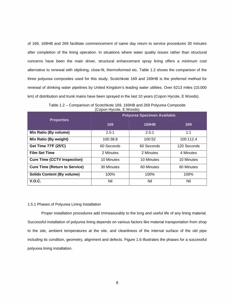
1.2 Comparison of Scotchkote 169, 169HB and 269 Polyurea Composite .................................................. 8
1.3 Physical Properties and Test Methods for Typical Polyurea Material (Copon Hycote, 2009) .............. 10
1.4 Features and Advantages of Polyurea Lining (Scotchkote 269 Coating, 2009) ................................... 11
2.1 Comparison of Conventional Technologies used in Coating Industry (Primeaux II, 2000) .................. 19
2.2 Typical Ovality Factor ‘C’ for Partially and Fully Deteriorated Conditions ............................................ 31
2.3 Coefficients for Four Parameter Equations at 20oC (Lacroix, et.al, 2007) ............................................ 32
2.4 Bending Creep Modulus at Different Times (Lin, 1995) ........................................................................ 33
2.5 Tensile Creep Modulus at Different Times (Lin, 1995) ......................................................................... 33
2.6 Flexural Creep, Deflection & Strain for Specimen 1 (Knight, 2005) ..................................................... 34
2.7 Flexural Creep, Deflection & Strain for Specimen 2 (Knight, 2005) ..................................................... 34
2.8 Creep Modulus at 10,000 hours and Estimated 50-year Modulus (Knight, 2005) ................................ 35
3.1 Dial Gauge Specifications ..................................................................................................................... 47
4.1 Load Selection for Various Polyurea Specimens .................................................................................. 52
4.2 Summary of Measured Tensile Strain at Various Time Intervals.......................................................... 53
4.3 Summary of Short-term Tensile Modulus for the Polyurea Composite ................................................ 55
4.4 Summary of Measured Tensile Modulus ET at Various Time Intervals ................................................ 55
4.5 Load Selection for Various Polyurea Specimens .................................................................................. 59
4.6 Summary of Measured Flexural Strain at Various Time Intervals ........................................................ 60
4.7 Summary of Short-term Flexural Modulus for the Polyurea Composite ............................................... 62
4.8 Summary of Measured Flexural Modulus EF at Various Time Intervals ............................................... 63
4.9 Coefficients for Flexural Creep using Log-Curve Fitting Method .......................................................... 67
4.10 Comparison of Experimental and Theoretical Flexural Strain % ........................................................ 68
xi
4.11 Coefficients for Tensile Creep using Log Curve Fitting Method ......................................................... 68
4.12 Comparison of Experimental and Theoretical Tensile Strain % ......................................................... 69
4.13 Findley’s Coefficient ‘m’ & ‘n’ for Tensile Creep Test ......................................................................... 73
4.14 Comparison of Tensile Creep Strain Theoretical and Experimental ................................................... 74
4.15 Findley’s Coefficient ‘m’ & ‘n’ for Tensile Creep Test ......................................................................... 77
4.16 Comparison of Flexural Creep Strain Theoretical and Experimental ................................................. 78

1
CHAPTER 1
INTRODUCTION
1.1 Background
Pipeline systems have been in use for more than a century and most of them are deteriorated
significantly and are in need for repair, renewal or replacement. Renewal of existing water pipe systems
worldwide using “trenchless technology” has become popular over the past few decades. Trenchless
technology is a rapidly growing industry that eliminates or reduces the need for surface excavation, often
referred to as “NO-DIG” technology. Any pipe material is subjected to deterioration and subsequent
failure due to many factors, such as, corrosion, age, pipe environment, climate, operational factors and so
on. According to ASTM, a deteriorated pipeline is classified into partially or fully deteriorated. Partially
deteriorated pipe can carry soil and surcharge load, but is unable to resist hydrostatic loads. In fully
deteriorated condition, the pipe is present but is no longer considered to support the soil and the
surcharge loads. This research focuses on a new trenchless renewal method, using polyurea as a lining
material to extend the service life of the partially deteriorated potable water pipes. Polyurea is a lining
material applied to the interior surface of the deteriorated host pipe using spray technique. It is applied to
enhance the structural ability of the pipeline. For this research, commercially available polyurea
composites by 3M Water Infrastructure are used under the names Scotchkote 169, Scotchkote 169HB
and Scotchkote 269 are used.
Scotchkote 169, 169HB (formerly known by Copon Hycote brand) was developed by E. Wood, Ltd.,
in the United Kingdom. E. Woods developed this revolutionary spray on application and rapid setting
polymeric product for the semi-structural renewal of potable water pipes for long-term protection and to
address problems of water discoloration and odor. Scotchkote 169, 169HB and 269 are two component
resins specifically designed for use in internal pipeline applications. These products can be applied to
pipelines that may have been considered for replacement, due to their age or overall conditions.

2
1.2 Current State of Water Systems
Renewal and maintenance of buried pipes is a major challenge faced by engineers, utility owners,
and decision makers due to ageing pipes and increasing gap in funding. The U.S. Environmental
Protection Agency (EPA) estimates that nearly $1 trillion is needed in critical drinking water and
wastewater investments over the next two decades (ASCE Report, 2009). Efficient management of these
funds will require tools that managers and decision makers can employ to optimally allocate funds and
prioritize infrastructure improvements (Juhl et al, 1994 & Deb, et al, 1999).
The deterioration rate of buried pipes is a function of many factors such as material, age, soil
condition, and hydraulic parameters of the fluids inside these pipes. It is usually the cumulative effects of
these different factors rather than each individual factor that determines the condition of the pipe (Figure
1.1).
Figure 1.1 - Effects of Tuberculation, Age and Corrosion on Water Pipes (Source: 3M Water Infrastructure)
According to a report by the American Water Works Association (AWWA), both internal and
external forces on the water main have major effects on its expected useful life (AWWA, 2001). Figure 1.2
is an example of deterioration rate over time for water pipes.
3
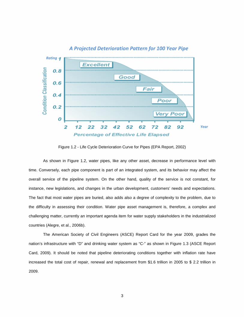
Figure 1.2 - Life Cycle Deterioration Curve for Pipes (EPA Report, 2002)
As shown in Figure 1.2, water pipes, like any other asset, decrease in performance level with
time. Conversely, each pipe component is part of an integrated system, and its behavior may affect the
overall service of the pipeline system. On the other hand, quality of the service is not constant, for
instance, new legislations, and changes in the urban development, customers’ needs and expectations.
The fact that most water pipes are buried, also adds also a degree of complexity to the problem, due to
the difficulty in assessing their condition. Water pipe asset management is, therefore, a complex and
challenging matter, currently an important agenda item for water supply stakeholders in the industrialized
countries (Alegre, et al., 2006b).
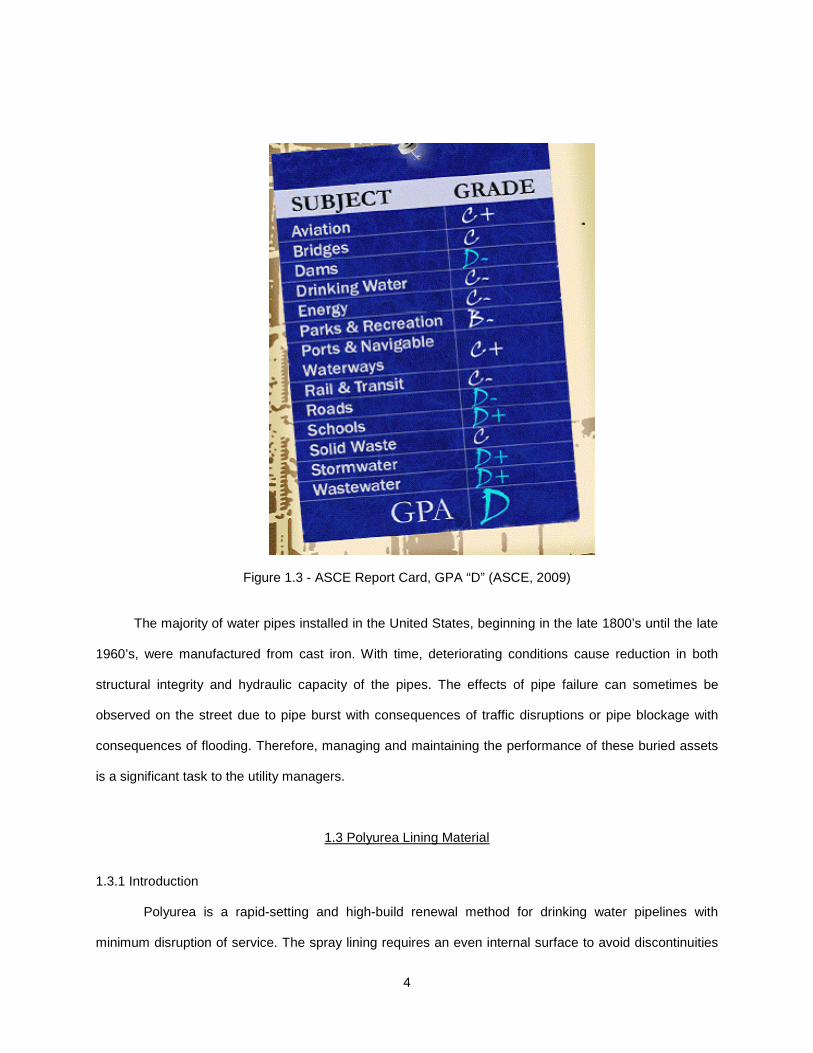
The American Society of Civil Engineers (ASCE) Report Card for the year 2009, grades the
nation’s infrastructure with “D” and drinking water system as “C-” as shown in Figure 1.3 (ASCE Report
Card, 2009). It should be noted that pipeline deteriorating conditions together with inflation rate have
increased the total cost of repair, renewal and replacement from $1.6 trillion in 2005 to $ 2.2 trillion in
2009.
A Projected Deterioration Pattern for 100 Year Pipe
Year
Rating
4
Figure 1.3 - ASCE Report Card, GPA “D” (ASCE, 2009)
The majority of water pipes installed in the United States, beginning in the late 1800’s until the late
1960’s, were manufactured from cast iron. With time, deteriorating conditions cause reduction in both
structural integrity and hydraulic capacity of the pipes. The effects of pipe failure can sometimes be
observed on the street due to pipe burst with consequences of traffic disruptions or pipe blockage with
consequences of flooding. Therefore, managing and maintaining the performance of these buried assets
is a significant task to the utility managers.
1.3 Polyurea Lining Material
1.3.1 Introduction
Polyurea is a rapid-setting and high-build renewal method for drinking water pipelines with
minimum disruption of service. The spray lining requires an even internal surface to avoid discontinuities

5
at joint areas thus ensuring optimum thickness of linings throughout the length of the application. The
lining is formed using centrifugal application equipment. The end result is a high build inert and corrosion
resistant lining system. The speed of application results in rapid renewal of water pipes with quick return
to service.
Polyurea lining is a trenchless technology method, leading to minimum social costs and
disturbances to adjacent utilities and structures, as well as minimum surface and subsurface excavations.
With conventional open-cut construction methods, direct costs are greatly increased with need to restore
ground surfaces such as sidewalks, pavement, landscaping, and so on (Najafi & Gokhale, 2005).
Additionally, social and environmental factors related to open-cut methods include adverse impacts on
the community, businesses, and commuters due to air pollution, noise and dust, safety hazards and traffic
disruptions. Polyurea linings can renew and enhance water pipes with addressing the following problems
as per “Scotchkote 269 Design Guide”:
1. Pipeline Internal Corrosion Problems:
Polyurea lining provides a highly effective and corrosion-resistant barrier coating within the pipe
surface.
2. Water Quality Problems Associated with Pipeline Internal Corrosion:
Lining resists any tuberculation which contributes to conveyed water quality problems. In addition, the
smooth surface of lining prevents the formation of other pipe deposits (Figure 1.4).
Figure 1.4 - Finished Polyurea Spray Lining
6
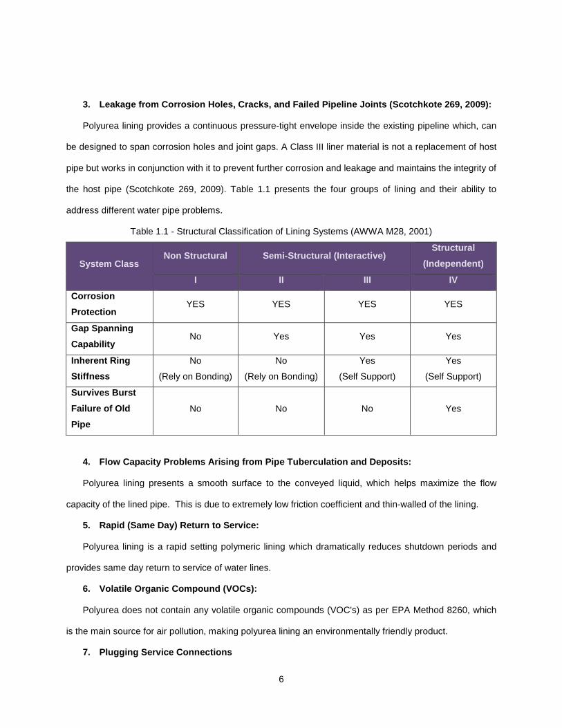
3. Leakage from Corrosion Holes, Cracks, and Failed Pipeline Joints (Scotchkote 269, 2009):
Polyurea lining provides a continuous pressure-tight envelope inside the existing pipeline which, can
be designed to span corrosion holes and joint gaps. A Class III liner material is not a replacement of host
pipe but works in conjunction with it to prevent further corrosion and leakage and maintains the integrity of
the host pipe (Scotchkote 269, 2009). Table 1.1 presents the four groups of lining and their ability to
address different water pipe problems.
Table 1.1 - Structural Classification of Lining Systems (AWWA M28, 2001)
System Class Non Structural Semi-Structural (Interactive)
Structural
(Independent)
I II III IV
Corrosion
Protection YES YES YES YES
Gap Spanning
Capability No Yes Yes Yes
Inherent Ring
Stiffness
No
(Rely on Bonding)
No
(Rely on Bonding)
Yes
(Self Support)
Yes
(Self Support)
Survives Burst
Failure of Old
Pipe
No No No Yes
4. Flow Capacity Problems Arising from Pipe Tubercu lation and Deposits:
Polyurea lining presents a smooth surface to the conveyed liquid, which helps maximize the flow
capacity of the lined pipe. This is due to extremely low friction coefficient and thin-walled of the lining.
5. Rapid (Same Day) Return to Service:
Polyurea lining is a rapid setting polymeric lining which dramatically reduces shutdown periods and
provides same day return to service of water lines.
6. Volatile Organic Compound (VOCs):
Polyurea does not contain any volatile organic compounds (VOC's) as per EPA Method 8260, which
is the main source for air pollution, making polyurea lining an environmentally friendly product.
7. Plugging Service Connections
7
During installation process, polyurea lining eliminates the need for blocking of service connections.
Rapid curing process thus eliminates the need for providing temporary bypass connection to the
customer.
8. Structural Integrity and Design Life of Old Pipe :
Polyurea Class III lining structurally renews the old pipe with a giving a new design life.
1.4 History of Polyurea
Polyurea is a name given to a wide range of polymeric material that has extensively been used in
the coating industry in solid elastomeric or rigid form. Introduced in 1989 by Texaco Chemical Company,
polyurea was regarded as a product that did not fulfill the exaggerated expectations initially advertised,
especially in the coating industry. Recent studies, however, have shown promising mechanical responses
for polyurea that are not limited to only the coating applications but venture into critical applications such
as reinforcement of metal structures against blast and impact loads (Alireza et.al, 2004).
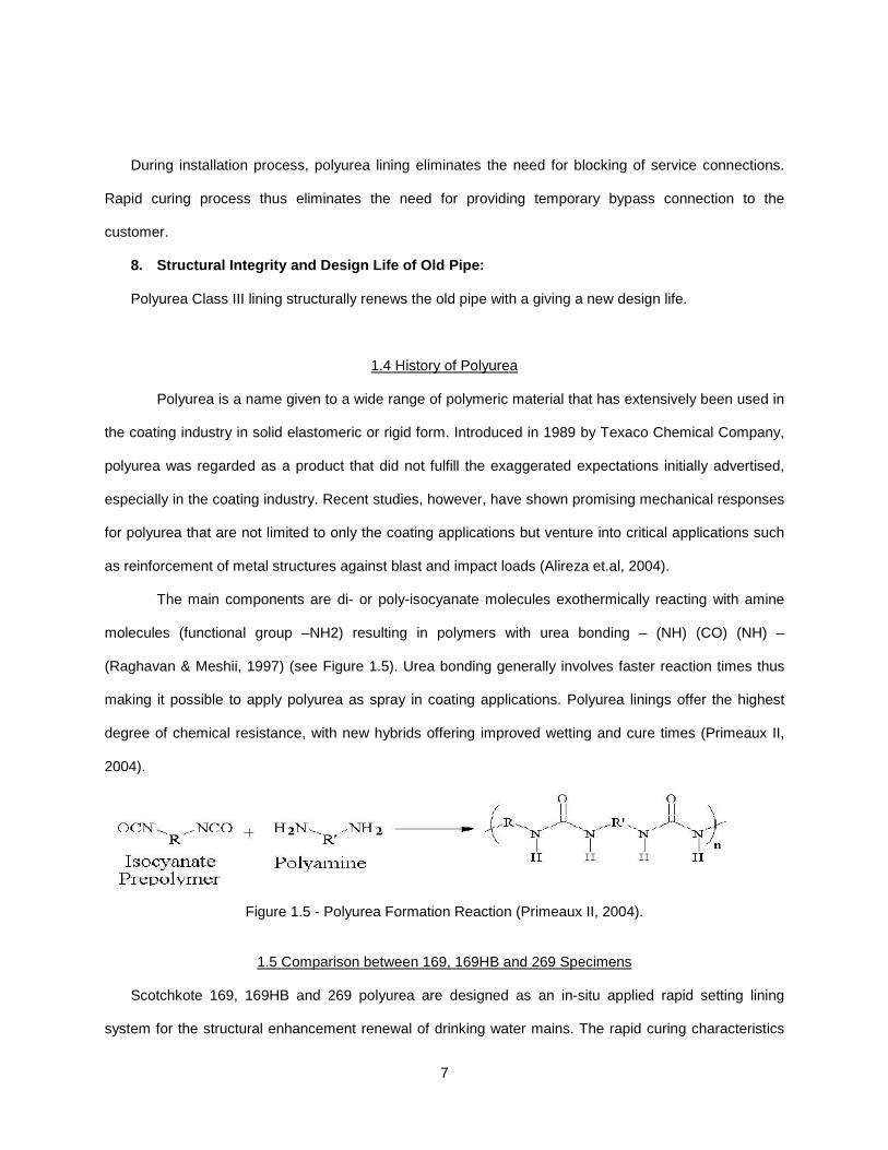
The main components are di- or poly-isocyanate molecules exothermically reacting with amine
molecules (functional group –NH2) resulting in polymers with urea bonding – (NH) (CO) (NH) –
(Raghavan & Meshii, 1997) (see Figure 1.5). Urea bonding generally involves faster reaction times thus
making it possible to apply polyurea as spray in coating applications. Polyurea linings offer the highest
degree of chemical resistance, with new hybrids offering improved wetting and cure times (Primeaux II,
2004).
Figure 1.5 - Polyurea Formation Reaction (Primeaux II, 2004).
1.5 Comparison between 169, 169HB and 269 Specimens
Scotchkote 169, 169HB and 269 polyurea are designed as an in-situ applied rapid setting lining
system for the structural enhancement renewal of drinking water mains. The rapid curing characteristics
8
of 169, 169HB and 269 facilitate commencement of same day return to service procedures 30 minutes
after completion of the lining operation. In situations where water quality issues rather than structural
concerns have been the main driver, structural enhancement spray lining offers a minimum cost
alternative to renewal with sliplining, close-fit, thermoformed etc. Table 1.2 shows the comparison of the
three polyurea composites used for this study. Scotchkote 169 and 169HB is the preferred method for
renewal of drinking water pipelines by United Kingdom’s leading water utilities. Over 6213 miles (10,000
km) of distribution and trunk mains have been sprayed in the last 10 years (Copon Hycote, E Woods).
Table 1.2 – Comparison of Scotchkote 169, 169HB and 269 Polyurea Composite (Copon Hycote, E.Woods)
Properties Polyurea Specimen Available
169 169HB 269
Mix Ratio (By volume) 2.5:1 2.5:1 1:1
Mix Ratio (By weight) 100:38.8 100:52 100:112.4
Get Time 77°F (25°C) 60 Seconds 60 Seconds 120 Seconds
Film Set Time 2 Minutes 2 Minutes 4 Minutes
Cure Time (CCTV Inspection) 10 Minutes 10 Minutes 10 Minutes
Cure Time (Return to Service) 30 Minutes 60 Minutes 60 Minutes
Solids Content (By volume) 100% 100% 100%
V.O.C. Nil Nil Nil
1.5.1 Phases of Polyurea Lining Installation
Proper installation procedures add immeasurably to the long and useful life of any lining material.
Successful installation of polyurea lining depends on various factors like material transportation from shop
to the site, ambient temperatures at the site, and cleanliness of the internal surface of the old pipe
including its condition, geometry, alignment and defects. Figure 1.6 illustrates the phases for a successful
polyurea lining installation.
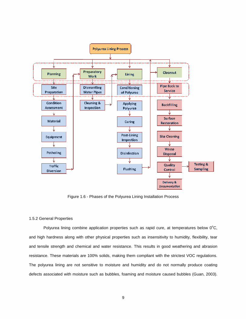
Figure 1.6 - Phases of the
1.5.2 General Properties
Polyurea lining combine application properties such as rapid cure,
and high hardness along with other
and tensile strength and chemical and water resistance.
resistance. These materials are 100% solids, making them compliant with the strictest VOC regulations.
The polyurea lining are not sensitive to moisture and humidity and do not normally produce coating
defects associated with moisture such as bubbles, foaming and moisture caused bubbles (Guan, 2003).
9
Phases of the Polyurea Lining Installation Process
olyurea lining combine application properties such as rapid cure, at temperatures below 0
other physical properties such as insensitivity to humidity,
and tensile strength and chemical and water resistance. This results in good weathering and abrasion
are 100% solids, making them compliant with the strictest VOC regulations.
tive to moisture and humidity and do not normally produce coating
defects associated with moisture such as bubbles, foaming and moisture caused bubbles (Guan, 2003).
at temperatures below 0oC,
insensitivity to humidity, flexibility, tear
weathering and abrasion
are 100% solids, making them compliant with the strictest VOC regulations.
tive to moisture and humidity and do not normally produce coating
defects associated with moisture such as bubbles, foaming and moisture caused bubbles (Guan, 2003).
10
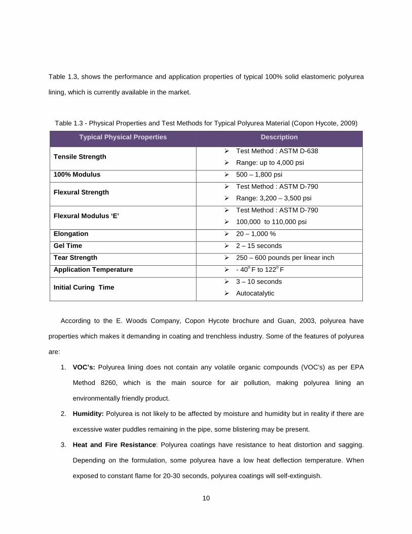
Table 1.3, shows the performance and application properties of typical 100% solid elastomeric polyurea
lining, which is currently available in the market.
Table 1.3 - Physical Properties and Test Methods for Typical Polyurea Material (Copon Hycote, 2009)
Typical Physical Properties Description
Tensile Strength � Test Method : ASTM D-638
� Range: up to 4,000 psi
100% Modulus � 500 – 1,800 psi
Flexural Strength � Test Method : ASTM D-790
� Range: 3,200 – 3,500 psi
Flexural Modulus ‘E’ � Test Method : ASTM D-790
� 100,000 to 110,000 psi
Elongation � 20 – 1,000 %
Gel Time � 2 – 15 seconds
Tear Strength � 250 – 600 pounds per linear inch
Application Temperature � - 40o F to 122o F
Initial Curing Time � 3 – 10 seconds
� Autocatalytic
According to the E. Woods Company, Copon Hycote brochure and Guan, 2003, polyurea have
properties which makes it demanding in coating and trenchless industry. Some of the features of polyurea
are:
1. VOC’s: Polyurea lining does not contain any volatile organic compounds (VOC's) as per EPA
Method 8260, which is the main source for air pollution, making polyurea lining an
environmentally friendly product.
2. Humidity: Polyurea is not likely to be affected by moisture and humidity but in reality if there are
excessive water puddles remaining in the pipe, some blistering may be present.
3. Heat and Fire Resistance : Polyurea coatings have resistance to heat distortion and sagging.
Depending on the formulation, some polyurea have a low heat deflection temperature. When
exposed to constant flame for 20-30 seconds, polyurea coatings will self-extinguish.
11
4. Waterproof : Seamless waterproofing system for concrete, metal, soil, and other substrates.
5. Abrasion Resistance: Polyurea has resistance to withstand mechanical action such as rubbing,
scraping, or erosion that tends progressively to remove material from its surface.
6. Elasticity : Polyurea being an elastomer has a very linear structure with much less cross-linking
which makes it stretchy and elastic.
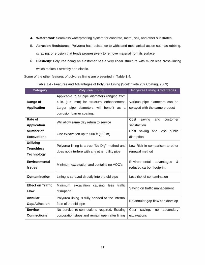
Some of the other features of polyurea lining are presented in Table 1.4.
Table 1.4 - Features and Advantages of Polyurea Lining (Scotchkote 269 Coating, 2009)
Category Polyurea Lining Polyurea Lining Advantages
Range of
Application
Applicable to all pipe diameters ranging from
4 in. (100 mm) for structural enhancement.
Larger pipe diameters will benefit as a
corrosion barrier coating.
Various pipe diameters can be
sprayed with the same product
Rate of
Application Will allow same day return to service
Cost saving and customer
satisfaction
Number of
Excavations One excavation up to 500 ft (150 m)
Cost saving and less public
disruption
Utilizing
Trenchless
Technology
Polyurea lining is a true “No-Dig” method and
does not interfere with any other utility pipe
Low Risk in comparison to other
renewal method
Environmental
Issues Minimum excavation and contains no VOC’s
Environmental advantages &
reduced carbon footprint
Contamination Lining is sprayed directly into the old pipe Less risk of contamination
Effect on Traffic
Flow
Minimum excavation causing less traffic
disruption Saving on traffic management
Annular
Gap/Adhesion
Polyurea lining is fully bonded to the internal
face of the old pipe No annular gap flow can develop
Service
Connections
No service re-connections required. Existing
corporation stops and remain open after lining
Cost saving, no secondary
excavations

12
1.6 Need Statement
Water pipe performance reduces gradually with time, resulting in high maintenance cost, poor
water quality, leakage problems and loss of pressure. Structural and leakage problems are common in
old cast iron water mains, particularly in pipe larger than 30 in. (760 mm). The majority of these problems
are caused by some combination of corrosion, soil movements, traffic loads, and operating pressures.
About 50% of water pipes in the North American water systems are of cast iron, unlined and are installed
prior to 1950s. Many of these water pipes are structurally sound, but show tuberculation, resulting in
reduction in hydraulic capacity and water quality issues (Figure 1.7) (AWWA, 2006).
Figure 1.7 - Intensity of Tuberculation Present (Source: 3M Water Infrastructure)
Spray lining methods such as cement mortar, epoxy and polyurethane have been used for number
years and have performed well in the water industry. Since polyurea is a new product available for the
renewal of corroded underground water pipes, it is necessary to develop an appropriate design procedure
for determining the strength of the lining material and to ensure that it is capable of spanning corrosion
holes without failing over a minimum design life. Therefore, it is important to know the physical and
mechanical properties, among which long-term tensile and flexural creep are the basic parameters which
will help to decide the life expectancy of the polyurea lining material. Not much research has been done in
13
the past in determination of long-term tensile and flexural strength of polyurea material, which is the basic
requirement in the prediction of the design life of this material.
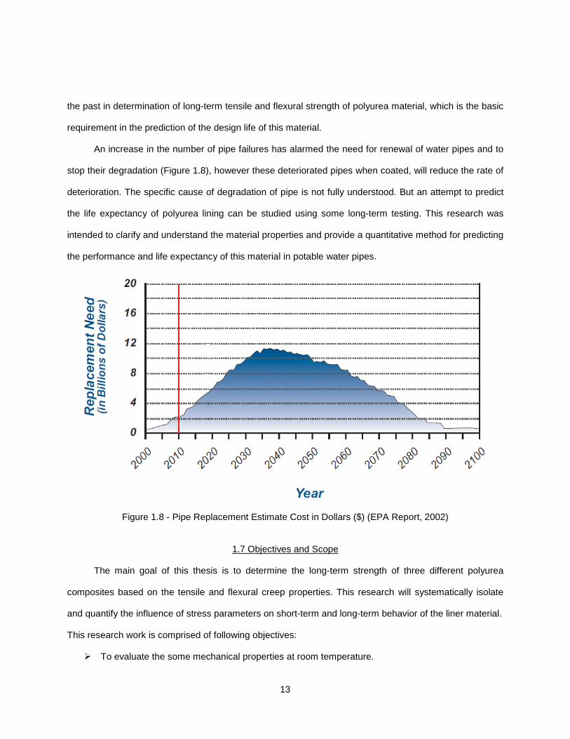
An increase in the number of pipe failures has alarmed the need for renewal of water pipes and to
stop their degradation (Figure 1.8), however these deteriorated pipes when coated, will reduce the rate of
deterioration. The specific cause of degradation of pipe is not fully understood. But an attempt to predict
the life expectancy of polyurea lining can be studied using some long-term testing. This research was
intended to clarify and understand the material properties and provide a quantitative method for predicting
the performance and life expectancy of this material in potable water pipes.
Figure 1.8 - Pipe Replacement Estimate Cost in Dollars ($) (EPA Report, 2002)
1.7 Objectives and Scope
The main goal of this thesis is to determine the long-term strength of three different polyurea
composites based on the tensile and flexural creep properties. This research will systematically isolate
and quantify the influence of stress parameters on short-term and long-term behavior of the liner material.
This research work is comprised of following objectives:
� To evaluate the some mechanical properties at room temperature.
14
� Perform trial test with similar setup to determine the appropriate stress value for long-term test.
� Perform test on the liner material such as long-term tensile and flexural creep and formulate
results.
� Model experimental creep strain responses using Findley’s Power Law.
� Model the experimental creep strain responses using log fitting curve.
� Predict long-term properties and design life of polyurea composite.
1.8 Research Methodology
The research is based on analyzing the mechanical properties of polyurea composite such as
tensile and flexural creep, its behavior and effect, when subjected to long-term continuous and constant
loading. Creep takes into account the total deformation under stress after a specific time at a given
temperature. This property is very useful in the design of pipe liners. To attain these mechanical
properties the following tests are conducted:
1.8.1 Long-term Tests
1.8.1.1 Tensile Creep Test
The research works investigates the long-term tensile creep properties and report the following
information:
� Performing test for 1,000 hours and determining stress value for long-term test.
� Applying constant load to a dumbbell shaped polyurea 169, 169HB & 269 specimens and
measuring its elongation as a function of time.
� Recording strain response using strain gages attached to the specimens and measured
elongation at time intervals of 1, 6, 12, 30 min; 1, 2, 5, 20, 50, 100, 200, 500, 700 and 1,000
hours.
� Carrying out the testing at room temperature.
� Testing the specimens for approximately 1,000 hours or until failure whichever comes first.
15
1.8.1.2 Flexural Creep Test
The research works investigates the long-term flexural creep properties and report the following
information:
� Performing test for 1,000 hours and determining stress value for long-term test.
� Applying constant load to polyurea 169, 169HB & 269 specimens and measuring its flexural
strength as a function of time.
� Measuring the deflection of the specimen at mid-span using accurate deflection gauges.
� Recording the deflection of the specimen at time intervals of 1, 6, 12, 30 min; 1, 2, 5, 20, 50, 100,
200, 500, 700 and 1,000 hours. Plotting the percent creep strain against time.
� Carrying out the testing at room temperature.
� Testing the specimens for approximately 1,000 hours or until failure whichever comes first
(approx 2 months).
1.8.1.3 Modeling and Predicting Design Life
Time dependent deformation of a material under sustained load is referred to as creep. If the load is
large and the duration is long, failure (i.e., creep-rupture) will occur. Since the duration of test is shorter,
following models are used to extrapolate the results.
� Predicting the design life based on results obtained from 1,000 hour creep test and extrapolation
it as described in ASTM D 2990 to ensure design of least 50-year.
� Developing a long-term design model using curve fitting method, and predicting the strain
response for various specimens and comparing with other models.
� Modeling the creep strain by using Findley’s Power law to extrapolate strain to 50-year and
predict the reduction in strength.
� Evaluating and comparing the percent increase in strain over 50-year using curve fitting and
Findley’s law.

16
1.9 Structure of the Thesis
The main challenge in understanding the behavior of polyurea material in potable water pipes is the
speed of degradation. The life expectancy of this material is a very slow process and testing with service
conditions within the laboratory time frame requires large number of results. Hence, it is common practice
in the creep testing to test more samples by varying the temperature and stress.
Chapter 1 introduces the current situation of buried pipes with statistical results showing the past,
present and the future status of pipeline system. Also, it discusses the need of renewal of water pipe
system, and also the cost associated with failure of these pipelines. Additionally, with some advantages,
and benefits of using polyurea lining compared to other spray-on liners currently being used. It provides
an overview of the objective of this thesis, the need statement and the expected outcome of this work.
Chapter 2 explains the literature review, methods of long-term performance curves generation from
short-term experimental results. It also provides an overview of polyurea application in pipe lining
industry. This chapter also highlights some of the past research on creep carried out with summary of
results. Also, explaining some of the research carried out and method developed to determine the creep
behavior of materials.
Chapter 3 discusses all the laboratory tests, test set-ups, test procedures according to ASTM and
ISO standards and their significance in mechanical characterization of the polyurea composite. It also,
explains the experimental setup, with figures of the setup and procedure for recording the readings.
Chapter 4 discusses experiments long-term tensile and flexure test with results, figures, tables and
discussions. Additionally, the calculations for the data obtained are also shown in this chapter. It also
evaluates the experimental results to predict the design life Findley’s Power Law and Log-Fitting curve
method. The results provide an understanding of liner behavior and will help of creep models in predicting
the design life of the liner. Finally, Chapter 5 discusses the conclusions and recommendations for future
work.
1.10 Expected Outcome
From the testing point of view, polyurea can prove to be an effective method in gap spanning and
corrosion protection by providing some design life to the host pipe. Also this material cannot be
17
considered to be a class IV liner (i.e. structural liner) but can provide some structural enhancement to the
host pipe.
Some of the other outcomes from this thesis are highlighted below:
� A theoretical analysis of the experimental data using creep models.
� A simple comparison of the experimental and theoretical analysis data in predicting the
design life.
1.11 Chapter Summary
This chapter provides an overview of current state of water system and a trenchless solution
using polyurea lining renewal method. The chapter also gives a brief introduction on polyurea lining
material with its material properties and advantages in trenchless applications. The most significant
obstacle preventing the extensive use of polyurea lining is lack of long-term performance data, such as
creep testing. The objectives, scope, need statement and expected outcome of this thesis is also
highlighted in this chapter.
19
CHAPTER 2
LITERATURE REVIEW
2.1 Introduction to Polymers
The most basic component of elastomeric material is polymer. The word polymer is derived from
the Greek term “many parts.” Polymers are large molecules of repeated units called monomers
chemically bond into long chains. Elastomeric materials consist of relatively long polymeric chains having
a high degree of flexibility and mobility. When subjected to external stresses, these long chains may alter
their configuration rather rapidly because of the high chain mobility. Polymeric materials are available in
variety of forms. They may be available in the form of solid of varying hardness, liquid or dispersed in
water as latex. Some are converted into finished product and some are modified to provide desired result.
In the last few decades, polymeric materials have been widely used in many industrial
applications, especially in pipe coatings (Guidetti, et al., 1996; Harris and Lorenz, 1993; Kamimura and
Kishikawa, 1998; Leng, et al., 1986). Recently, the lining based on polymer such as polyurethane, epoxy
and polyurea became more and more dominant in the pipe lining. They represent a durable, high
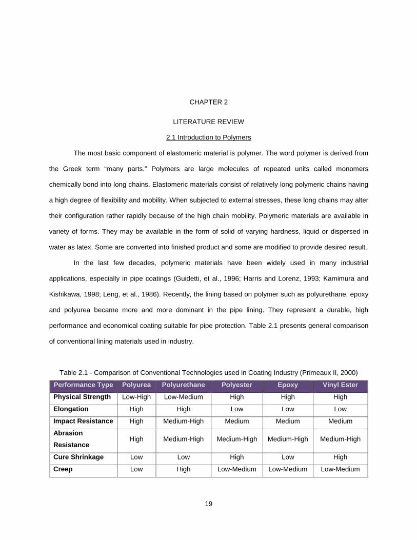
performance and economical coating suitable for pipe protection. Table 2.1 presents general comparison
of conventional lining materials used in industry.
Table 2.1 - Comparison of Conventional Technologies used in Coating Industry (Primeaux II, 2000)
Performance Type Polyurea Polyurethane Polyester Epoxy Vinyl Ester
Physical Strength Low-High Low-Medium High High High
Elongation High High Low Low Low
Impact Resistance High Medium-High Medium Medium Medium
Abrasion
Resistance High Medium-High Medium-High Medium-High Medium-High
Cure Shrinkage Low Low High Low High
Creep Low High Low-Medium Low-Medium Low-Medium
20
However, the use of polymer in a variety of aggressive environments such as corrosive
environments, humidity, wide range of temperature, etc. can affect their lifetime, provoking the
deterioration of their physical and mechanical properties. Study of this deterioration is time consuming; it
may take several years to obtain any result. So, the comprehension of ageing mechanism and prediction
of service life of polymeric coatings require convenient laboratory tests, which effectively speeds up the
changes resulting from the critical weathering conditions and provides a quick indication of weather
resistance (Guermazia, et.al, 1997). One of the most important aspects of long-term durability and
dimensional stability of polyurea material is their long-term creep behavior. Prediction of long-term
integrity of any polymeric composite structure depends on the viscoelastic properties of these materials
(Raghavan & Meshii, 1997).
2.2 Creep Properties and Theories
Creep is defined as increase in strain with time at a constant stress level. When a plastic material
is subjected to a sustained load, it deforms continuously. The initial strain is roughly predicted by its
stress-strain modulus. The material will continue to deform slowly with time indefinitely or until rupture or
yielding causes failure. The primary region is the early stage of loading when the creep rate decreases
rapidly with time. Then it reaches a steady state which is called the secondary creep stage followed by a
rapid increase called the tertiary stage and finally results in break. Some materials do not have secondary
stage, while tertiary creep only occurs at high stresses and for ductile materials. All plastics creep to a
certain extent. The degree of creep depends on several factors, such as type of plastic, magnitude of
load, temperature and time (Pomeroy, 1978). In polymers, creep occurs due to a combination of elastic
deformation and viscous flow of polymer molecules, commonly known as viscoelastic deformation (Park &
Balatinez, 1998).
2.2.1 Effect of Temperature and Humidity on Creep
Temperature and humidity can significantly affect the
resulting in physical and mechanical changes in
polymer is cooled from an elevated temperature at which the molecular mobility is high to a lower
temperature at which relaxation times for molecular motions are long in comparison with the storage time
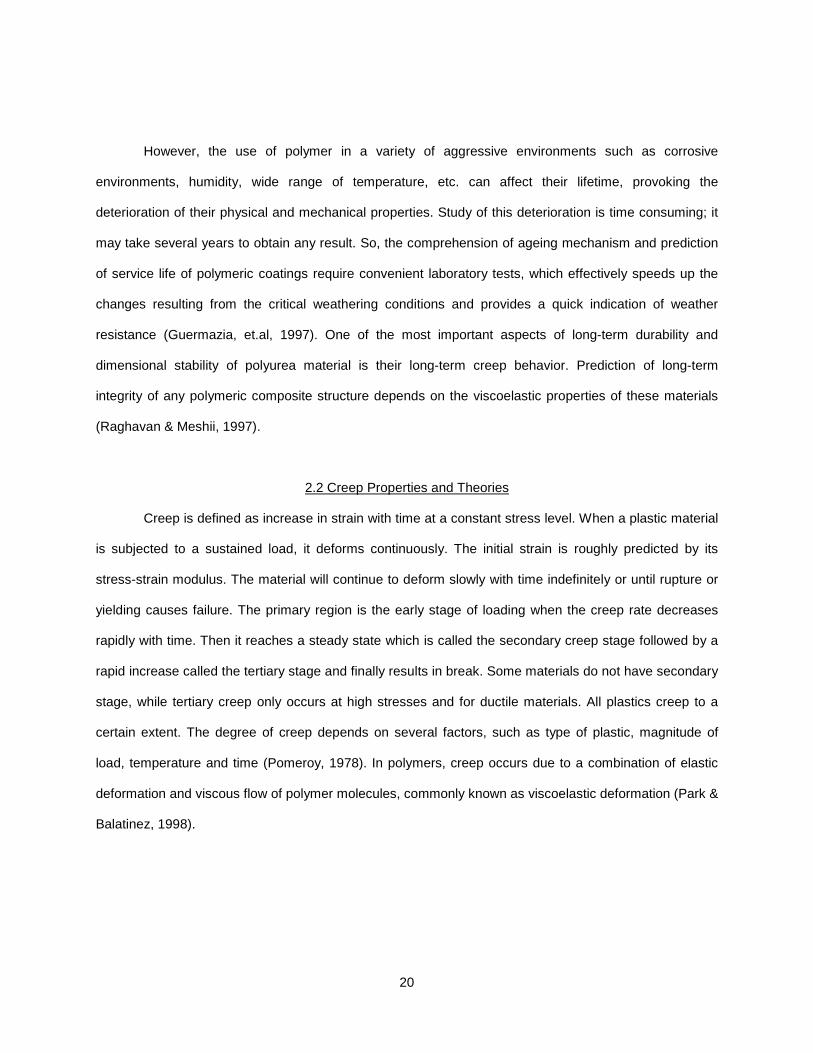
at that temperature (Riande, 2000). The effect of temperature on the response of creep behavior can be
quantitatively observed in Figure 2.1
With the ageing process, there is a progressive decrease in the molecular mobility of the polymer
at constant temperature. As a result, the creep deformation produced by an applied constant stress will
depend upon the age of the polymer, resulting in lower creep rate in highly aged materials
2003). Generally, moisture absorption level is history dependent; hen
different for varying temperatures (Batra, 2009). However, the
the actual ageing time; thus, no significant ag
Figure 2.1 - Influence of Temperat
21
erature and Humidity on Creep
Temperature and humidity can significantly affect the deterioration process of the polymer
resulting in physical and mechanical changes in material properties. Physical ageing takes place when a
polymer is cooled from an elevated temperature at which the molecular mobility is high to a lower
temperature at which relaxation times for molecular motions are long in comparison with the storage time
. The effect of temperature on the response of creep behavior can be
1.
With the ageing process, there is a progressive decrease in the molecular mobility of the polymer
ure. As a result, the creep deformation produced by an applied constant stress will
depend upon the age of the polymer, resulting in lower creep rate in highly aged materials
Generally, moisture absorption level is history dependent; hence the moisture absorption will be
(Batra, 2009). However, the creep test time will be
ing time; thus, no significant ageing will occur during the test.
Influence of Temperature on the Strain of Creep Experiment (Riande et.al, 2000)
process of the polymer
properties. Physical ageing takes place when a
polymer is cooled from an elevated temperature at which the molecular mobility is high to a lower
temperature at which relaxation times for molecular motions are long in comparison with the storage time
. The effect of temperature on the response of creep behavior can be
With the ageing process, there is a progressive decrease in the molecular mobility of the polymer
ure. As a result, the creep deformation produced by an applied constant stress will
depend upon the age of the polymer, resulting in lower creep rate in highly aged materials (ISO 899-2,
ce the moisture absorption will be
much shorter than
(Riande et.al, 2000)

In practical use, however, loading cycles are not so short, and ag
cycle and temperature variations. Determination of how ag
materials is critical to the use of polymers. Depending on the region of viscoelastic behavior, the
mechanical properties of polymers differ greatly. Model stress
illustrated in Figure 2.2.
Figure 2.2 - Stress–S
2.2.2 Time - Temperature Superposition
There currently exist no reliable methods and techniques to predict directly the long
behavior of polymer (Ding & Wang, 2007). There are
place in polymer under natural ageing conditions, occurring very slowly. In order to speed up this ageing
condition, high temperatures are often used to
demonstrate these changes that occur during accelerated ageing and compare them to the changes that
occur during natural ageing at ambient conditions (Erhardt and Mecklenburg
Superposition (TTS) was first noticed experimentally in the late 1930s in a study of viscoelastic behavior
in polymers and polymer fluids (Vinogradov, 1980 & Tobolsky, 1967)
22
In practical use, however, loading cycles are not so short, and ageing occurs during the loading
cycle and temperature variations. Determination of how ageing affects the long-term
materials is critical to the use of polymers. Depending on the region of viscoelastic behavior, the
mechanical properties of polymers differ greatly. Model stress–strain behavior for various polymer types
Strain Behavior of Various Polymers (Riande, et.al, 2000)
Temperature Superposition
There currently exist no reliable methods and techniques to predict directly the long
(Ding & Wang, 2007). There are many chemical and physical changes that take
under natural ageing conditions, occurring very slowly. In order to speed up this ageing
condition, high temperatures are often used to accelerate the changes. It therefore becomes necessary to
se changes that occur during accelerated ageing and compare them to the changes that
occur during natural ageing at ambient conditions (Erhardt and Mecklenburg, 1995). Time
first noticed experimentally in the late 1930s in a study of viscoelastic behavior
Vinogradov, 1980 & Tobolsky, 1967). Further studies indicated that the
ing occurs during the loading
response of such
materials is critical to the use of polymers. Depending on the region of viscoelastic behavior, the
for various polymer types is
(Riande, et.al, 2000)
There currently exist no reliable methods and techniques to predict directly the long-term ageing
many chemical and physical changes that take
under natural ageing conditions, occurring very slowly. In order to speed up this ageing
therefore becomes necessary to
se changes that occur during accelerated ageing and compare them to the changes that
1995). Time-Temperature
first noticed experimentally in the late 1930s in a study of viscoelastic behavior
. Further studies indicated that the
23
TTS could be explained theoretically by some molecular structure models (Ding, et.al 1979). It
has been shown experimentally that the elastic modulus (E) of a polymer is influenced by the dynamic
loading and the response time.
Time-temperature superposition implies that the response time function of the elastic modulus at
a certain temperature resembles the shape of the same functions of adjacent temperatures. Curves of
elastic modulus (E) vs. log (response time) at one temperature can be shifted to overlap with adjacent
curves. The amount of shifting along the horizontal (x-axis) in a typical TTS plot requires to align the
individual experimental data points on the master curve and is generally described using one of two
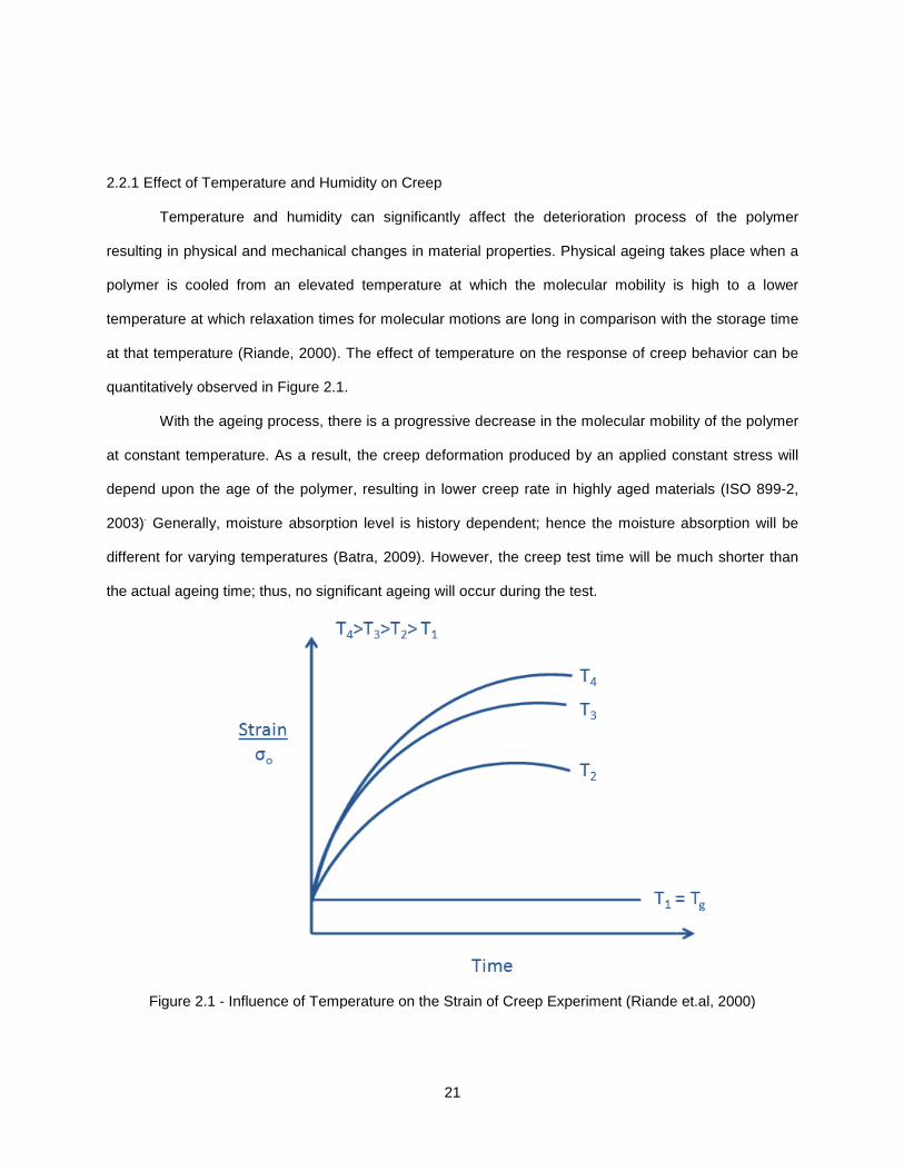
common theoretical models. The first of these models is the Williams-Landel-Ferry (WLF) using Equation
2.1 (Ferry, 1980):
1 0
2 0
( )
( )t
C T TLog A
C T T
− −=
+ − Equation 2.1
Where,
C1 and C2 = Constants,
T0 = Reference Temperature (K),
T = Measurement Temperature (K),
At = Shift Factor.
The WLF equation is typically used to describe the time/temperature behavior of polymers in the
glass transition region. The equation is based on the assumption that, above the glass transition
temperature, the fractional free volume increases linearly with respect to temperature (Williams, et.al,
1955). The model also assumes that as the free volume of the material increases, its viscosity rapidly
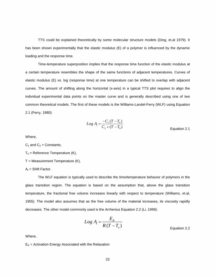
decreases. The other model commonly used is the Arrhenius Equation 2.2 (Li, 1999):
( )R
to
ELog A
R T T=
− Equation 2.2
Where,
ER = Activation Energy Associated with the Relaxation
R = Gas Constant,
T = Measurement Temperature,
T0 = Reference Temperature,
At = Shift Factor.
The Arrhenius equation is typically used to describe behavior outside
but has also been used to obtain the activation energy associated with the glass transition.
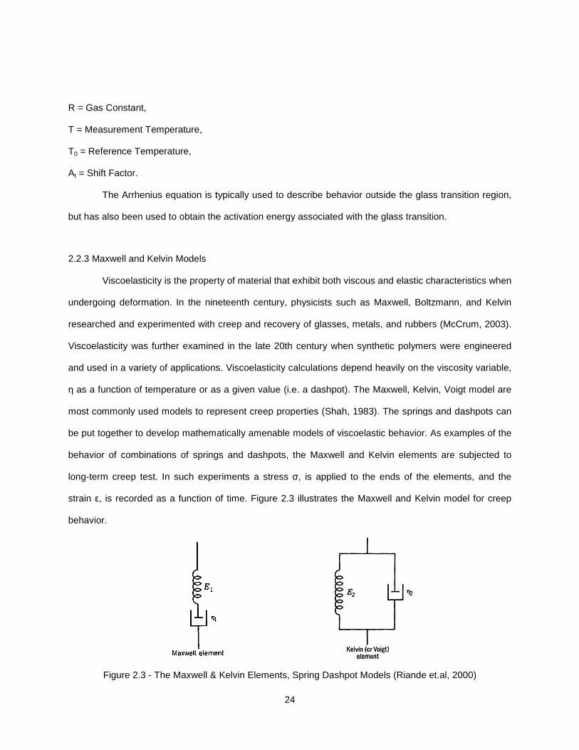
2.2.3 Maxwell and Kelvin Models
Viscoelasticity is the property of material that exhibit both viscous and elastic characteristics wh
undergoing deformation. In the nineteenth century, physicists such as
researched and experimented with
Viscoelasticity was further examined in the late 20th century when synthetic polymers were engineered
and used in a variety of applications. Viscoelasticity calculations depend heavily on the viscosity variable,
η as a function of temperature or as a given value (i.e
most commonly used models to represent creep properties
be put together to develop mathematically amenable models of viscoelastic behavior. As examples of the
behavior of combinations of springs and dashpots, the Maxwell and Kelvin elements are subjected to
long-term creep test. In such experiments a stress
strain ε, is recorded as a function of time. Figure 2.
behavior.
Figure 2.3 - The Maxwell &
24
The Arrhenius equation is typically used to describe behavior outside the glass transition region,
but has also been used to obtain the activation energy associated with the glass transition.
is the property of material that exhibit both viscous and elastic characteristics wh
In the nineteenth century, physicists such as Maxwell, Boltzmann
researched and experimented with creep and recovery of glasses, metals, and rubbers
was further examined in the late 20th century when synthetic polymers were engineered
and used in a variety of applications. Viscoelasticity calculations depend heavily on the viscosity variable,
as a function of temperature or as a given value (i.e. a dashpot). The Maxwell, Kelvin, Voigt model
most commonly used models to represent creep properties (Shah, 1983). The springs and dashpots can
be put together to develop mathematically amenable models of viscoelastic behavior. As examples of the
r of combinations of springs and dashpots, the Maxwell and Kelvin elements are subjected to
term creep test. In such experiments a stress σ, is applied to the ends of the elements, and the
, is recorded as a function of time. Figure 2.3 illustrates the Maxwell and Kelvin model for creep
Kelvin Elements, Spring Dashpot Models (Riande et.al, 2000)
the glass transition region,
but has also been used to obtain the activation energy associated with the glass transition.
is the property of material that exhibit both viscous and elastic characteristics when
Boltzmann, and Kelvin
rubbers (McCrum, 2003).
was further examined in the late 20th century when synthetic polymers were engineered
and used in a variety of applications. Viscoelasticity calculations depend heavily on the viscosity variable,
The Maxwell, Kelvin, Voigt model are
. The springs and dashpots can
be put together to develop mathematically amenable models of viscoelastic behavior. As examples of the
r of combinations of springs and dashpots, the Maxwell and Kelvin elements are subjected to
, is applied to the ends of the elements, and the
rates the Maxwell and Kelvin model for creep
(Riande et.al, 2000)
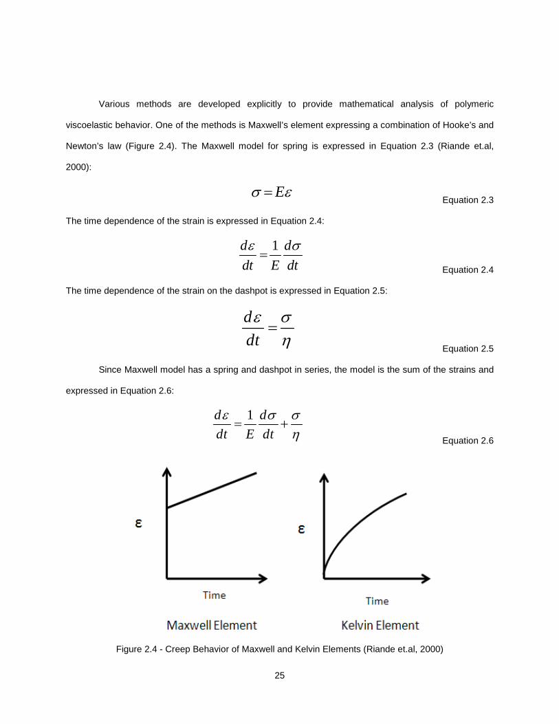
25
Various methods are developed explicitly to provide mathematical analysis of polymeric
viscoelastic behavior. One of the methods is Maxwell’s element expressing a combination of Hooke’s and
Newton’s law (Figure 2.4). The Maxwell model for spring is expressed in Equation 2.3 (Riande et.al,
2000):
Eσ ε= Equation 2.3
The time dependence of the strain is expressed in Equation 2.4:
1d d
dt E dt
ε σ=
Equation 2.4
The time dependence of the strain on the dashpot is expressed in Equation 2.5:
d
dt
ε ση
= Equation 2.5
Since Maxwell model has a spring and dashpot in series, the model is the sum of the strains and
expressed in Equation 2.6:
1d d
dt E dt
ε σ ση
= + Equation 2.6
Figure 2.4 - Creep Behavior of Maxwell and Kelvin Elements (Riande et.al, 2000)
26
The main limitation of the Maxwell model is that it does not give a good prediction of the long-
term behavior of the polymer. The creep behavior of the polymer cannot be represented accurately by
only one exponential decay time. But the model gives a very good representation of the creep behavior at
very short times. The Kelvin-Voigt element expresses a combination of spring and dashpot in parallel.
The Kelvin-Voigt model can be represented in Equation 2.7 (Riande, et.al, 2000):
( )( ) ( )
d tt E t
dt
η εσ ε= +
Equation 2.7
Where,
σ = Experimental Stress, psi
= Strain that Occurs under the given Stress,
E = Elastic Modulus of the Material
= Viscosity of the Material
2.2.4 Findley model
A common experimental approach is the one proposed by Findley W.N. (1987), which was used
successfully to predict the creep behavior up to 26 years. The tensile creep process is governed by
several factors and number of methods, has been proposed to describe the tensile creep behavior of
plastics in terms of stress (psi), strain (%) and loading time (hrs). Findley W.N (1944) has proposed a
generalized discussion on the mechanisms of creep in complex linear polymer, amorphous and
crystalline polymers. He also showed that creep data for a number of thermoplastic materials can be
represented by Equation 2.8 (Findley, 1944).
( ) not mtε ε= + Equation 2.8
Where,
ε(t) = Sum of Elastic Strain and Time Dependent Strain (Function of Stress)
εo = Time-independent Strain
m = Coefficient of the Time-dependent Term (Function of Stress)

27
n = Constant for a Given Material Independent of Stress
t = Elapsed Time of Loading (hours).
In the structural evaluation of polymer liners, it is very important to investigate the short-term and
long-term elastic modulus EL of the material very precisely. Most polymer exhibit large creep strains at
room temperature and at low stress levels. At higher temperature or large stresses, creep behavior
becomes more critical. Generally, highly cross-linked thermoset polymers exhibit lower creep strains as
compared to thermoplastics (Mallick, 2008). Miller and Sterrett (1988) have examined eleven analytical
expressions used for creep data and reported to what extent they fitted experimental data available in
literature. The material investigated were acetal, acrylonitrile butadiene styrene (ABS), Nylon 6/6,
Polyethylene (PE), Polypropylene (PP), Poly Vinyl Chloride (PVC), Polyurethane (PU) and thermoplastic
Polyurethane Elastomer (TPUE) (Lacroix, et. al, 2007). The data obtain from creep test are often used for
the design life prediction of the material under elevated or specific temperature. They provide relationship
between the rupture time (hrs), stress (psi) and temperature (oC) (Aktaa & Schinke, 1996).
2.2.5 Boltzmann-Volterra Superposition Principle
The Boltzmann–Volterra linear hereditary creep theory is commonly used for characterizing the
time-dependent properties of viscoelastic materials (Riande, 2000). The stress-strain relationship in the
simplest loading case of creep is given by Equation 2.9 (Maksimov, et. al. 1975):
0
( )( ) ( )
t
o t
dJ t J t d
d
σ τε σ τ τ
τ= + −∫ Equation 2.9
Where,
Jo = Time independent Creep Compliance
Jt = Time Dependent Creep Compliance.
2.3 Use of Standards on Design and Testing
There are several test methods for evaluating long term properties of materials, including ASTM
D 2990, ISO 899-1-03, and ASTM F1216.

28
2.3.1 ASTM D2990-01
ASTM D2990-01 Standard Test Methods for Tensile, Compressive and Flexural Creep and Creep
Rupture of Plastics describe the measurement of creep and creep-rupture properties of plastics under
specific environmental conditions, mainly temperature and humidity. The method is a good reference as it
describes the test apparatus and calculations, includes the background discussion on basic concepts.
The standard outlines the test procedure for determining the long-term tensile & flexural creep modulus.
While the ASTM specification governing these tests does not specifically state an amount of time that
samples must remain under load.
2.3.2 ISO 899-1-03
ISO 899 Parts 1 and 2 address the same subject, but differ in technical content (and results
cannot be directly compared between the two test methods). ISO 899 Part 1 addresses tensile creep and
creep to rupture and ISO 899 Part 2 addresses flexural creep. Compressive creep is not addressed in
ISO 899. ASTM D2990 does not specify the test load for the samples, whereas ISO specifications also do
not specify the test loads for the samples. ISO standard 889-2 2003 states to select a stress value
appropriate to the application envisaged for the material under test or choose the stress such that the
deflection is not greater than 0.1 times the distance between the supports at any time during the test.
ISO 899-1-03 Plastics – Determination of Creep Behavior – Part 1: Tensile Creep is discusses
method for determining the tensile creep of plastics in the form of standard test specimens under
specified conditions such as those of pretreatment, temperature, and humidity. The method is suitable for
use with rigid and semi-rigid non-reinforced, filled and fiber-reinforced plastics materials in the form of
dumb-bell-shaped test specimens molded directly or machined from sheets or molded articles.
ISO 899-2-03 Plastics – Determination of Creep Behavior – Part 2: Flexural Creep by three-point
loading specifies a method for determining the flexural creep of plastics in the form of standard test
specimens under specified conditions such as those of pretreatment, temperature, and humidity.
29
2.3.3 ASTM F1216 Design Principle
ASTM F 1216-2009 describes the procedure for the renewal of pipelines and conduits in 4 to 108
in. (100 to 2,700 mm) diameters by the installation of a resin-impregnated, flexible tube which is inverted
into the existing conduit by use of a hydrostatic head or air pressure. This reconstruction process can be
used in a variety of gravity and pressure applications such as sanitary sewers, storm sewers, process
piping, electrical conduits, and ventilation systems. F 1216 design equations are often used for evaluating
the design parameters for successful renewal of pipes. Polyurea is a different material compared to CIPP;
however, general design equations can still remain the same with some modifications. The appendix in
the ASTM standard provides the design criteria for design partially and fully deteriorated pipe conditions
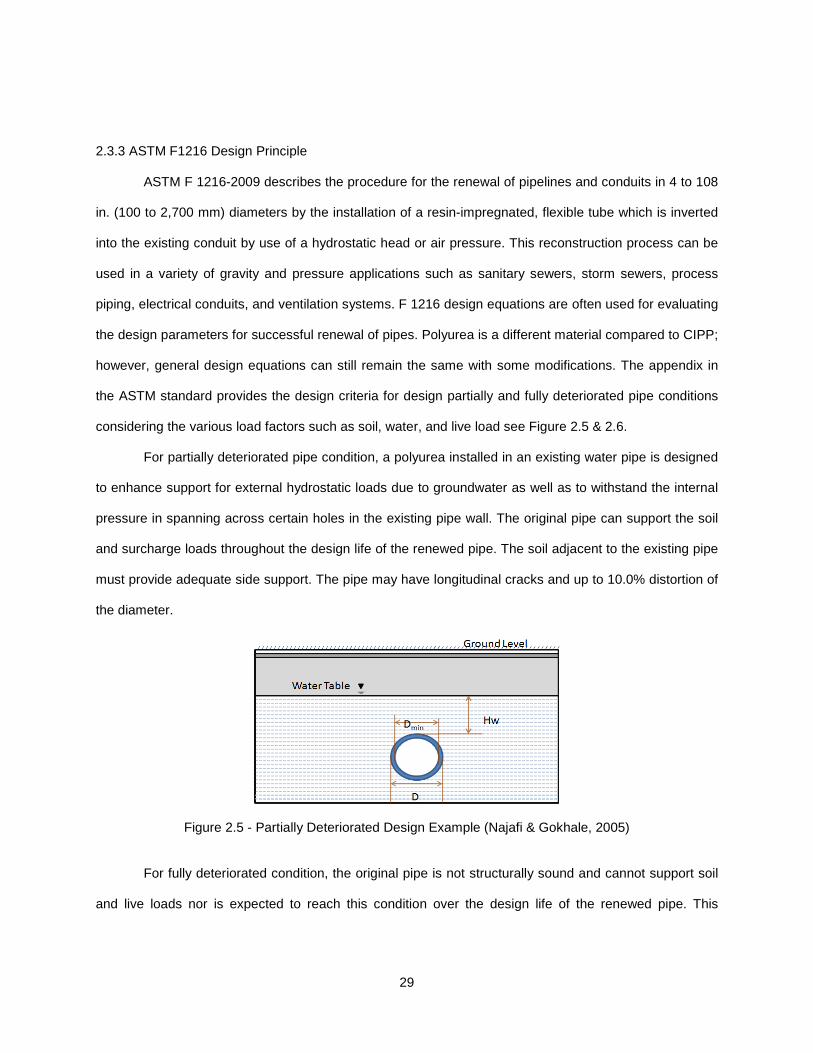
considering the various load factors such as soil, water, and live load see Figure 2.5 & 2.6.
For partially deteriorated pipe condition, a polyurea installed in an existing water pipe is designed
to enhance support for external hydrostatic loads due to groundwater as well as to withstand the internal
pressure in spanning across certain holes in the existing pipe wall. The original pipe can support the soil
and surcharge loads throughout the design life of the renewed pipe. The soil adjacent to the existing pipe
must provide adequate side support. The pipe may have longitudinal cracks and up to 10.0% distortion of
the diameter.
Figure 2.5 - Partially Deteriorated Design Example (Najafi & Gokhale, 2005)
For fully deteriorated condition, the original pipe is not structurally sound and cannot support soil
and live loads nor is expected to reach this condition over the design life of the renewed pipe. This
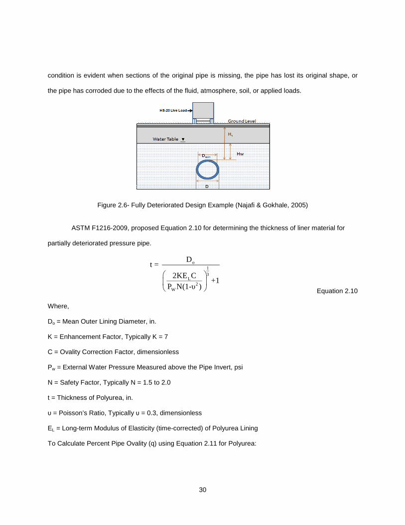
30
condition is evident when sections of the original pipe is missing, the pipe has lost its original shape, or
the pipe has corroded due to the effects of the fluid, atmosphere, soil, or applied loads.
Figure 2.6- Fully Deteriorated Design Example (Najafi & Gokhale, 2005)
ASTM F1216-2009, proposed Equation 2.10 for determining the thickness of liner material for
partially deteriorated pressure pipe.
o1
3L
2W
Dt =
2KE C+1
P N(1-υ )
Equation 2.10
Where,
Do = Mean Outer Lining Diameter, in.
K = Enhancement Factor, Typically K = 7
C = Ovality Correction Factor, dimensionless
Pw = External Water Pressure Measured above the Pipe Invert, psi
N = Safety Factor, Typically N = 1.5 to 2.0
t = Thickness of Polyurea, in.
υ = Poisson’s Ratio, Typically υ = 0.3, dimensionless
EL = Long-term Modulus of Elasticity (time-corrected) of Polyurea Lining
To Calculate Percent Pipe Ovality (q) using Equation 2.11 for Polyurea:

31
Mean Diameter - Minimum Diameterq = 100
Mean Diameter × Equation 2.11
To calculate Ovality Reduction Factor (C) for Polyurea using Table 2.2:
Table 2.2 - Typical Ovality Factor ‘C’ for Partially and Fully Deteriorated Conditions
Ovality q, % 0.0 1.0 2.0 4.0 5.0 6.0 8.0 10.0
Factor C 1.00 0.91 0.84 0.70 0.64 0.59 0.49 0.41
Selection of EL, long-term modulus of elasticity for polyurea composite is one of the objectives of
this study. The selection of EL depends on the design life of the material, for example if the design life of
this material is 50 years, corresponding value of EL will be for that period of time.
2.4 Past Research on Lining
Over the past decades, many researchers have carried out a great deal of research works on the
ageing of polymer materials obtaining some good results (Joachim, et.al, 1999). The behavior of liner
materials encased in a host pipe is complex to analyze. To study the liner behavior under varying internal
pressure and vacuum, it is important to investigate the influence of these different parameters on material
behavior. Polymer materials are known to exhibit viscoelastic behavior, i.e. creep. Polymer liner
performance is affected by creep behavior of the material. Creep strains in polymers its matrix are
dependent upon the percent of creep rupture stress induced in a member and temperature. However,
there is very little published data demonstrated especially how liner products perform over an extended
period of time under actual service conditions (Thomson, et.al. 1995).
Several methods of predicting the long-time deformation properties of polymeric materials are
now known (Urzhumtsev, 1971). These methods are primarily based on the mathematical modeling of the
creep process with subsequent extrapolation on a series of experimentally established analogies such as
superposition. Several investigations have presented different approaches to creep characterization
(Findley & Gautam, 1956). Generally approaches to determine the creep behavior of polymer can be
32
divided into theoretical and experimental methods. In the 19th century, physicists such as Maxwell,
Boltzmann, and Kelvin have researched and experimented with creep and recovery of rubbers.
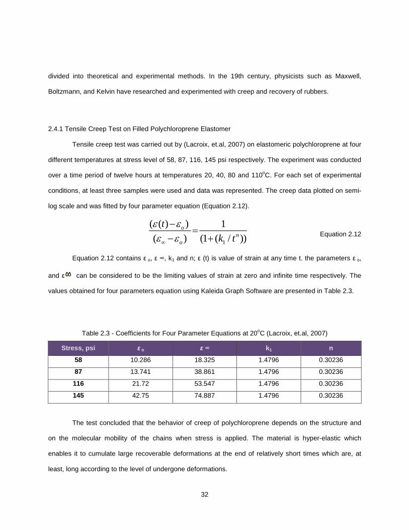
2.4.1 Tensile Creep Test on Filled Polychloroprene Elastomer
Tensile creep test was carried out by (Lacroix, et.al, 2007) on elastomeric polychloroprene at four
different temperatures at stress level of 58, 87, 116, 145 psi respectively. The experiment was conducted
over a time period of twelve hours at temperatures 20, 40, 80 and 110oC. For each set of experimental
conditions, at least three samples were used and data was represented. The creep data plotted on semi-
log scale and was fitted by four parameter equation (Equation 2.12).
1
( ( ) ) 1
( ) (1 ( / ))o
no
t
k t
ε εε ε∞
−=
− + Equation 2.12
Equation 2.12 contains ε o, ε ∞, k1 and n; ε (t) is value of strain at any time t. the parameters ε o,
and ε can be considered to be the limiting values of strain at zero and infinite time respectively. The
values obtained for four parameters equation using Kaleida Graph Software are presented in Table 2.3.
Table 2.3 - Coefficients for Four Parameter Equations at 20oC (Lacroix, et.al, 2007)
Stress, psi ε o ε ∞ k1 n
58 10.286 18.325 1.4796 0.30236
87 13.741 38.861 1.4796 0.30236
116 21.72 53.547 1.4796 0.30236
145 42.75 74.887 1.4796 0.30236
The test concluded that the behavior of creep of polychloroprene depends on the structure and
on the molecular mobility of the chains when stress is applied. The material is hyper-elastic which
enables it to cumulate large recoverable deformations at the end of relatively short times which are, at
least, long according to the level of undergone deformations.

33
2.4.2 Creep Test of Cured-In-Place Pipe Material
Long-term tensile, compression and bending test was performed on Cured-in-Place-Pipe (CIPP)
for 3,000 hrs at Louisiana Tech University, Ruston. Findley’s equation, log-fit method was used as a
baseline to predict the life of CIPP material. ASTM F 1216-93 Standard Practice for Rehabilitation of
Existing Pipelines and Conduits by the Inversion and Curing of Resin Impregnated Tube is often used as
a basis for design of CIPP liner materials. The tests were conducted based on ASTM D 2990-77
Standard Test Method for Tensile Compressive and Flexural and Creep Rupture of Plastics.
The apparatus used were bending table, lever loading and support structures for conducting the
test. For the bending test four stress levels were selected 1,000 psi, 2,000 psi, 3,000 psi, 4,000 psi and
for each stress two specimens were tested and summary of results are presented in Table 2.6. Similarly,
for tensile test four stress levels were selected for the tests, 1,000 psi, 1,500 psi, 2,000 psi and 2,500 psi
and for each stress two specimens were tested and summary of results are presented in Table 2.4 & 2.5.
The results obtained from 3,000 hours testing done are as follows.
Table 2.4 - Bending Creep Modulus at Different Times (Lin, 1995)
Stress, psi Eo (psi) Et (psi) Et (psi) Et (psi)
0.0167 h 1 h 1000 h 3000 h
1,000 488,505 449,935 328,425 285,215
2,000 486,330 444,280 300,005 254,765
3,000 458,490 417,310 273,035 230,695
4,000 452,690 411,075 255,200 181,975
Table 2.5 - Tensile Creep Modulus at Different Times (Lin, 1995)
Stress, psi Eo (psi) Et (psi) Et (psi) Et (psi)
0.0167 h 1 h 1000 h 3000 h
1000 751,390 506,485 288,405 256,360
2000 510,255 393,095 258,390 243,745
3000 449,790 365,690 259,260 243,890
4000 374,970 337,270 255,635 239,685

34
The results obtained from the long-term testing of 3,000 hrs concluded that the flexural creep
modulus is 44.2% of short-term flexural elastic modulus. Similarly average tensile creep modulus is
37.7% of short-term tensile elastic modulus.
2.4.3 AQUA-PIPE Cured-in-Place-Pipe (CIPP) Resin Project
The Centre for the Advancement of Trenchless Technology (CATT) conducted a series long-term
on Cured-in-Place Pipe (CIPP) material for the City of Toronto. The long-term flexural tests were carried
out to determine the creep performance and the creep retention factor. The flexural creep test was
performed according to ASTM D 2990-01. The initial load selected for the test was 25% of yield stress
determined using ASTM D 790. Observed test data were use to predict the design life for 50-year (Knight,
2005).
Six test specimens were water jet cut from resin plate of approximately 3.63 in. (92.1 mm) long by
0.76 in. (19.2 mm) wide by 0.181 to 0.189 in. (4.8 mm to 4.6 mm) deep. The test results for two
specimens at 1,000, 3,000, 6,000 and 10,000 hrs are summarized and shown in Table 2.6 & Table 2.7.
Figures 2.7 and 2.8 show the vertical deflection and the creep modulus for the 10,000 hour of load
application.
Table 2.6 - Flexural Creep, Deflection & Strain for Specimen 1 (Knight, 2005)
Sample Time (hours) Deflection (mm) Strain ε (%) Creep Modulus E F (psi)
S1-1 1,000 1.041 0.49 175,588
S1-1 3,000 1.224 0.58 149,359
S1-1 6,000 1.346 0.64 135832
S1-1 10,000 1.461 0.69 125,202
Table 2.7 - Flexural Creep, Deflection & Strain for Specimen 2 (Knight, 2005)
Sample Time (hours) Deflection (mm) Strain ε (%) Creep Modulus E F (psi)
S1-2 1,000 1.486 0.70 128,469
S1-2 3,000 1.791 0.84 106,602
S1-2 6,000 1.918 0.90 99,542
S1-2 10,000 2.085 0.98 91,540
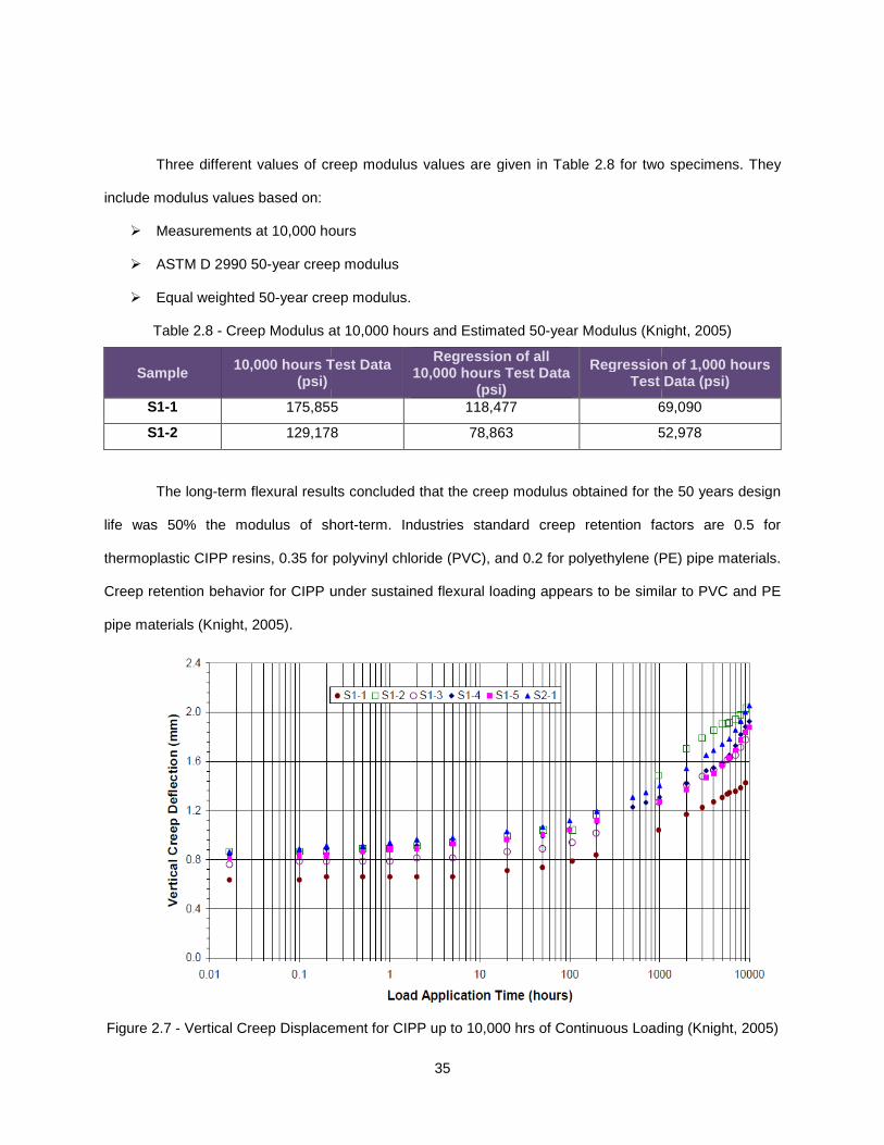
Three different values of creep modulus values are given in Table
include modulus values based on:
� Measurements at 10,000 hours
� ASTM D 2990 50-year creep modulus
� Equal weighted 50-year creep modulus.
Table 2.8 - Creep Modulus at 10,000
Sample 10,000 hours Test Data (psi)
S1-1 175,855
S1-2 129,178
The long-term flexural results
life was 50% the modulus of short
thermoplastic CIPP resins, 0.35 for polyvinyl
Creep retention behavior for CIPP under sustained flexural loading appears to be similar to PVC and PE
pipe materials (Knight, 2005).
Figure 2.7 - Vertical Creep Displacemen
35
Three different values of creep modulus values are given in Table 2.8 for two specimens. They
Measurements at 10,000 hours
year creep modulus
year creep modulus.
Creep Modulus at 10,000 hours and Estimated 50-year Modulus (Knight
10,000 hours Test Data
Regression of all 10,000 hours Test Data
(psi)
Regression of 1,000 hours Test Data (psi)
175,855 118,477 69,090
129,178 78,863 52,978
term flexural results concluded that the creep modulus obtained for the 50 years design
life was 50% the modulus of short-term. Industries standard creep retention factors are 0.5 for
thermoplastic CIPP resins, 0.35 for polyvinyl chloride (PVC), and 0.2 for polyethylene (PE) pipe materials.
Creep retention behavior for CIPP under sustained flexural loading appears to be similar to PVC and PE
Vertical Creep Displacement for CIPP up to 10,000 hrs of Continuous Loading
for two specimens. They
Knight, 2005)
Regression of 1,000 hours Test Data (psi)
69,090
52,978
the creep modulus obtained for the 50 years design
standard creep retention factors are 0.5 for
chloride (PVC), and 0.2 for polyethylene (PE) pipe materials.
Creep retention behavior for CIPP under sustained flexural loading appears to be similar to PVC and PE
f Continuous Loading (Knight, 2005)
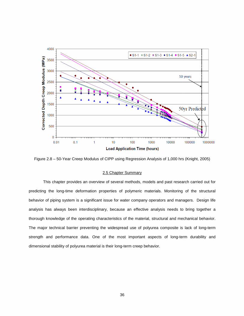
Figure 2.8 – 50-Year Creep Modulus
This chapter provides an overview of s
predicting the long-time deformation properties of p
behavior of piping system is a significant issue for water company operators and managers. Design life
analysis has always been interdisciplinary, because an effective analysis needs to bring together a
thorough knowledge of the operating characteristics of the material, structural and mechanical behavior.
The major technical barrier preventing the widespread use of polyurea composite is lack of long
strength and performance data.
dimensional stability of polyurea material is their long
36
Year Creep Modulus of CIPP using Regression Analysis of 1,000 hrs (
2.5 Chapter Summary
This chapter provides an overview of several methods, models and past research carried out
time deformation properties of polymeric materials. Monitoring of the structural
behavior of piping system is a significant issue for water company operators and managers. Design life
analysis has always been interdisciplinary, because an effective analysis needs to bring together a
h knowledge of the operating characteristics of the material, structural and mechanical behavior.
The major technical barrier preventing the widespread use of polyurea composite is lack of long
strength and performance data. One of the most important aspects of long-term durability and
dimensional stability of polyurea material is their long-term creep behavior.
0 hrs (Knight, 2005)
, models and past research carried out for
Monitoring of the structural
behavior of piping system is a significant issue for water company operators and managers. Design life
analysis has always been interdisciplinary, because an effective analysis needs to bring together a
h knowledge of the operating characteristics of the material, structural and mechanical behavior.
The major technical barrier preventing the widespread use of polyurea composite is lack of long-term
term durability and
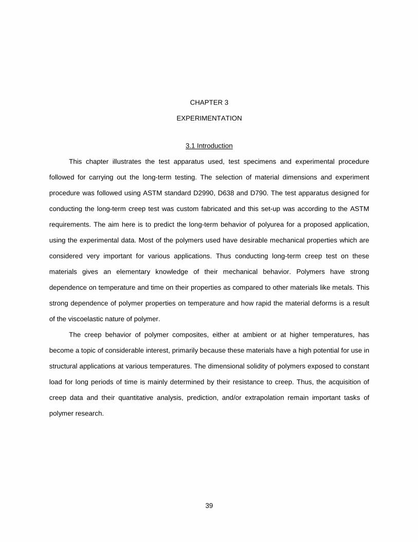
39
CHAPTER 3
EXPERIMENTATION
3.1 Introduction
This chapter illustrates the test apparatus used, test specimens and experimental procedure
followed for carrying out the long-term testing. The selection of material dimensions and experiment
procedure was followed using ASTM standard D2990, D638 and D790. The test apparatus designed for
conducting the long-term creep test was custom fabricated and this set-up was according to the ASTM
requirements. The aim here is to predict the long-term behavior of polyurea for a proposed application,
using the experimental data. Most of the polymers used have desirable mechanical properties which are
considered very important for various applications. Thus conducting long-term creep test on these
materials gives an elementary knowledge of their mechanical behavior. Polymers have strong
dependence on temperature and time on their properties as compared to other materials like metals. This
strong dependence of polymer properties on temperature and how rapid the material deforms is a result
of the viscoelastic nature of polymer.
The creep behavior of polymer composites, either at ambient or at higher temperatures, has
become a topic of considerable interest, primarily because these materials have a high potential for use in
structural applications at various temperatures. The dimensional solidity of polymers exposed to constant
load for long periods of time is mainly determined by their resistance to creep. Thus, the acquisition of
creep data and their quantitative analysis, prediction, and/or extrapolation remain important tasks of
polymer research.
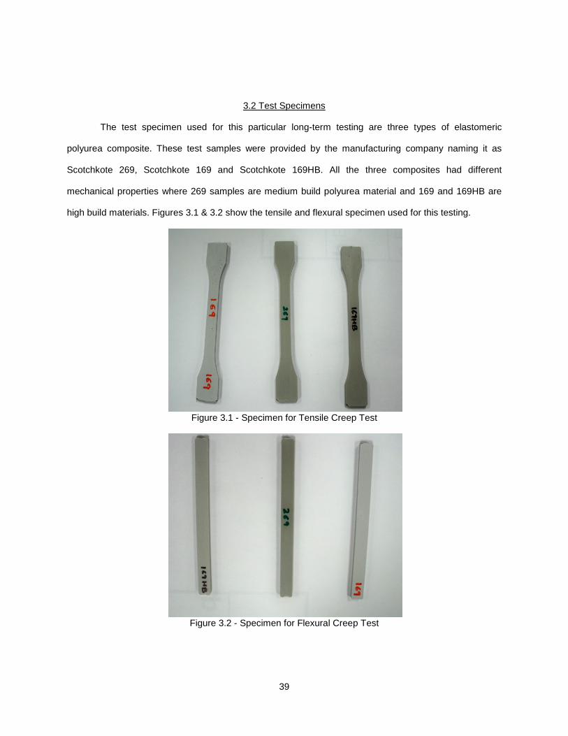
39
3.2 Test Specimens
The test specimen used for this particular long-term testing are three types of elastomeric
polyurea composite. These test samples were provided by the manufacturing company naming it as
Scotchkote 269, Scotchkote 169 and Scotchkote 169HB. All the three composites had different
mechanical properties where 269 samples are medium build polyurea material and 169 and 169HB are
high build materials. Figures 3.1 & 3.2 show the tensile and flexural specimen used for this testing.
Figure 3.1 - Specimen for Tensile Creep Test
Figure 3.2 - Specimen for Flexural Creep Test

40
3.3 Tensile Creep
3.3.1 Introduction
All polymeric material has a tendency to deform or “creep” when subjected to loading. The time-
dependence of such deformation behavior can be determined by standardization tests like tensile creep
and flexural creep tests. Among the most important mechanical properties of any elastomeric polymer
material, are tensile strength and tensile modulus. Tensile creep measurements are made by applying a
constant load on the test specimen and measuring its elongation with time. This elongation can be carried
out in several ways. The most accurate and simplest way is the use of strain gages which is capable of
measuring and amplifying small changes in length with time and directly plotting them on a graph paper.
The percent tensile creep strain is determined by dividing the change in length by the initial gage length
and multiplying by 100. The percent tensile creep is plotted against time to obtain a tensile creep curve.
The tensile strain values are determined at specified time intervals like 1, 6, 12, 30 min; 1, 5, 20, 50, 100,
500, 1,000 hours, to facilitate plotting a creep rupture curve.
3.3.2 Tensile Creep Apparatus
The apparatus designed for conducting the tensile creep test was custom fabricated and used a
simple loading mechanism at constant temperature. The test frame was designed using Mild Steel (MS)
angle frames of 2 in. x 2 in. (50 mm x 50 mm) machine welded. The table is designed to test 12
specimens with each sample bolted to MS square plates of 2 in. x 2 in. (50 mm x 50 mm). The plates
were chamfered from inside to hold the specimen avoid slippage during the experiment. Strain gages
were used to measure the strain at specific time intervals, according to ASTM D 2990 standard. The
strain gage selected for the test was EA-06-250BF-350 with a strain range of +5%. GAK-2-AE-10 strain
gage application kit was used to fix the strain gage to the specimen and was soldered to the terminal
wire. Strain gages were mounted axially along the length of the specimen as shown in Figure 3.3.
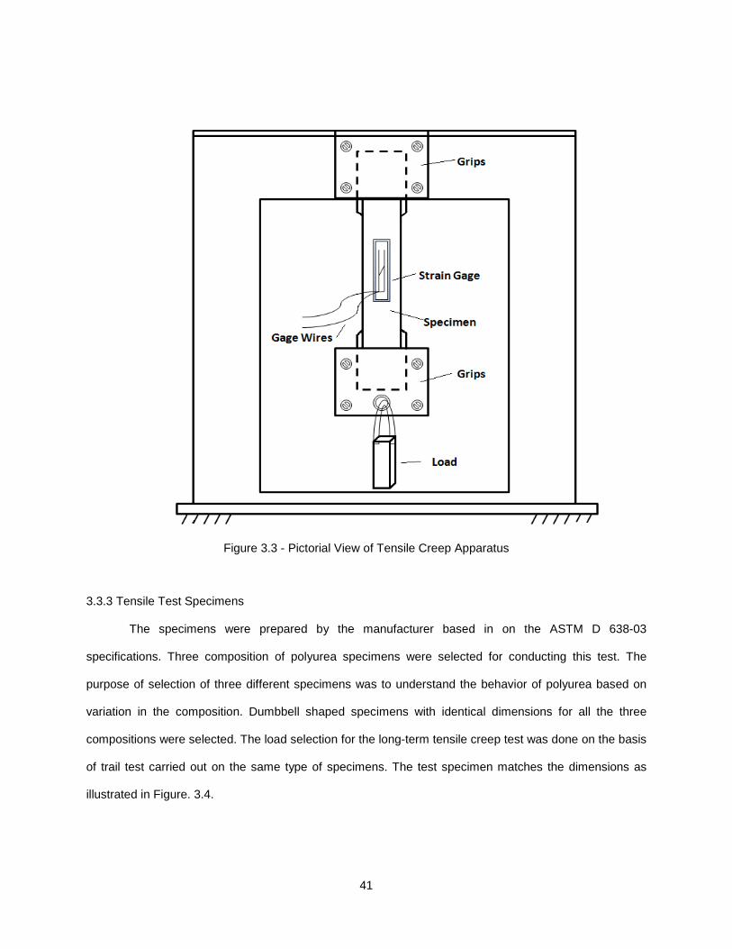
41
Figure 3.3 - Pictorial View of Tensile Creep Apparatus
3.3.3 Tensile Test Specimens
The specimens were prepared by the manufacturer based in on the ASTM D 638-03
specifications. Three composition of polyurea specimens were selected for conducting this test. The
purpose of selection of three different specimens was to understand the behavior of polyurea based on
variation in the composition. Dumbbell shaped specimens with identical dimensions for all the three
compositions were selected. The load selection for the long-term tensile creep test was done on the basis
of trail test carried out on the same type of specimens. The test specimen matches the dimensions as
illustrated in Figure. 3.4.
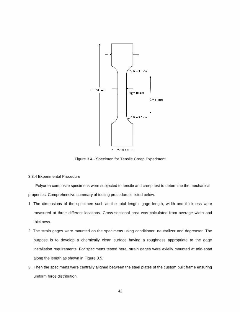
Figure 3.4
3.3.4 Experimental Procedure
Polyurea composite specimens were subjected to
properties. Comprehensive summary of testing
1. The dimensions of the specimen such as the total
measured at three different locations. Cross
thickness.
2. The strain gages were mounted on the specimens using conditioner, neutralizer and degreaser. The
purpose is to develop a chemically clean surface having a roughness appropriate to the gage
installation requirements. For specimens tested here, strain gages
along the length as shown in Figure 3.5
3. Then the specimens were centrally aligned between the steel plates of the custom built frame ensuring
uniform force distribution.
42
Figure 3.4 - Specimen for Tensile Creep Experiment
Polyurea composite specimens were subjected to tensile and creep test to determine the mechanical
properties. Comprehensive summary of testing procedure is listed below.
1. The dimensions of the specimen such as the total length, gage length, width and thickness were
measured at three different locations. Cross-sectional area was calculated from average width and
The strain gages were mounted on the specimens using conditioner, neutralizer and degreaser. The
is to develop a chemically clean surface having a roughness appropriate to the gage
installation requirements. For specimens tested here, strain gages were axially mounted at mid
as shown in Figure 3.5.
3. Then the specimens were centrally aligned between the steel plates of the custom built frame ensuring
and creep test to determine the mechanical
length, gage length, width and thickness were
sectional area was calculated from average width and
The strain gages were mounted on the specimens using conditioner, neutralizer and degreaser. The
is to develop a chemically clean surface having a roughness appropriate to the gage
were axially mounted at mid-span
3. Then the specimens were centrally aligned between the steel plates of the custom built frame ensuring

43
4. Strain gages were connected to the strain indicator unit with connecting wires.
5. Data was recorded for strain variations during the test. Experimental values of tensile strain and
modulus was calculated. This procedure was repeated for all the specimens.
6. Graphs of strain versus time for each specimen were plotted.
Figure 3.5 - Scotchkote 269 Specimen Tested for Tension
3.3.5 Tensile Creep Test Calculations
Tensile Stress (σ) - The tensile load applied per unit area of initial cross-section within the gauge length
(Equation 3.1).
( )( )
( )
Force PTensileStress
InitialCrossSectional Area Aσ = Equation 3.1
Where,
F = Applied Force, lbs
A = Average initial Cross-sectional Area within the Narrow (Gauge) Section of the Specimen, in2
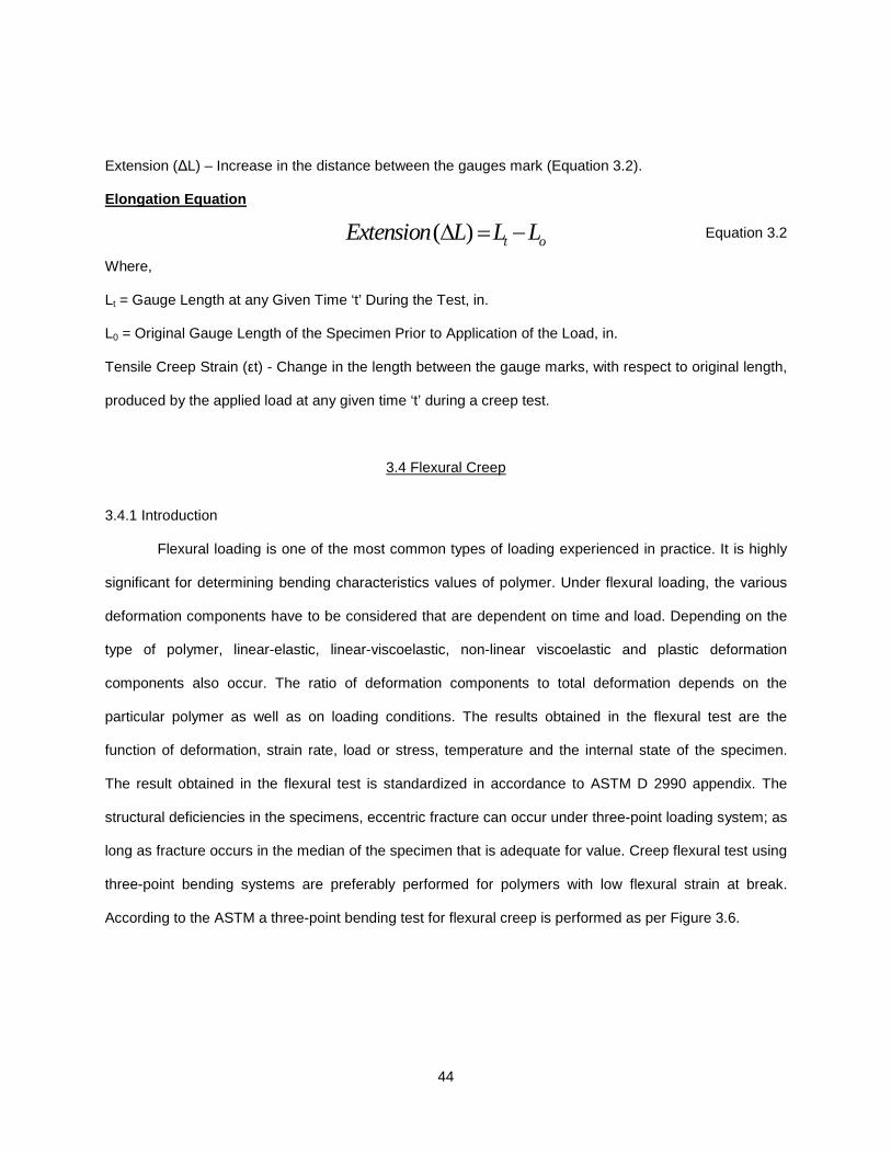
44
Extension (∆L) – Increase in the distance between the gauges mark (Equation 3.2).
Elongation Equation
Equation 3.2
Where,
Lt = Gauge Length at any Given Time ‘t’ During the Test, in.
L0 = Original Gauge Length of the Specimen Prior to Application of the Load, in.
Tensile Creep Strain (εt) - Change in the length between the gauge marks, with respect to original length,
produced by the applied load at any given time ‘t’ during a creep test.
3.4 Flexural Creep
3.4.1 Introduction
Flexural loading is one of the most common types of loading experienced in practice. It is highly
significant for determining bending characteristics values of polymer. Under flexural loading, the various
deformation components have to be considered that are dependent on time and load. Depending on the
type of polymer, linear-elastic, linear-viscoelastic, non-linear viscoelastic and plastic deformation
components also occur. The ratio of deformation components to total deformation depends on the
particular polymer as well as on loading conditions. The results obtained in the flexural test are the
function of deformation, strain rate, load or stress, temperature and the internal state of the specimen.
The result obtained in the flexural test is standardized in accordance to ASTM D 2990 appendix. The
structural deficiencies in the specimens, eccentric fracture can occur under three-point loading system; as
long as fracture occurs in the median of the specimen that is adequate for value. Creep flexural test using
three-point bending systems are preferably performed for polymers with low flexural strain at break.
According to the ASTM a three-point bending test for flexural creep is performed as per Figure 3.6.
( ) t oExtension L L L∆ = −

Figure 3.6
The maximum fiber stress for each specimen in
Where, S = Stress, psi,
P = Load, lbf,
L = Span, in.
b = Width, in.
d = Depth, in.
According to the ASTM the maximum strain in the outer fiber of the mid
ε (t)= Maximum strain, in./in.
∆ = Maximum deflection at mid-span, in.
d = Depth, in. and
L = Span, in.
Multiplying the strain ε(t) by 100 to obtain the percentage strain at specific time interval.
Flexural creep modulus for the specimen at any time during test is given by Equation 3.5:
45
6 - Schematic Diagram of Flexural Creep Test
The maximum fiber stress for each specimen in lb/in2 was calculated using Equation 3.3
According to the ASTM the maximum strain in the outer fiber of the mid-span is given by
span, in.
(t) by 100 to obtain the percentage strain at specific time interval.
Flexural creep modulus for the specimen at any time during test is given by Equation 3.5:
2
3. .
2. .
P L
b dσ =
2
6. .( )
dt
Lε
∆=
using Equation 3.3:
Equation. 3.3
span is given by Equation 3.4:
Equation 3.4
Flexural creep modulus for the specimen at any time during test is given by Equation 3.5:
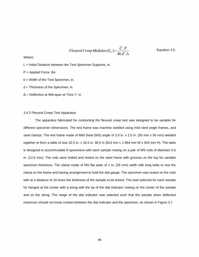
46
Equation 3.5.
Where;
L = Initial Distance between the Test Specimen Supports, in.
P = Applied Force, lbs
b = Width of the Test Specimen, in.
d = Thickness of the Specimen, in.
∆ = Deflection at Mid-span at Time ‘t’, in.
3.4.2 Flexural Creep Test Apparatus
The apparatus fabricated for conducting the flexural creep test was designed to be variable for
different specimen dimensions. The test frame was machine wielded using mild steel angle frames, and
steel clamps. The test frame made of Mild Steel (MS) angle of 2.0 in. x 2.0 in. (50 mm x 50 mm) wielded
together to form a table of size 32.5 in. x 34.5 in. 36.5 in (813 mm L x 864 mm W x 915 mm H). The table
is designed to accommodate 8 specimens with each sample resting on a pair of MS rods of diameter 0.5
in. (12.5 mm). The rods were bolted and rested on the steel frame with grooves on the top for variable
specimen thickness. The clamp made of MS flat plate of 1 in. (25 mm) width with long bolts to rest the
clamp on the frame and having arrangement to hold the dial gauge. The specimen was rested on the rods
with at a distance of 16 times the thickness of the sample to be tested. The load selected for each sample
for hanged at the center with a string with the tip of the dial indicator resting on the center of the sample
and on the string. The range of the dial indicator was selected such that the sample when deflected
maximum should not loose contact between the dial indicator and the specimen, as shown in Figure 3.7.
3
3
.( )
4 . .F
L PFlexural Creep Modulus E
b d=
∆

47
Figure 3.7 - Schematic View of Central Point Bending Setup
An accurate dial gauge (Table 3.1) was mounted on the clamp with the tip of the gauge resting on the
center of the polyurea specimen.
Table 3.1 - Dial Gauge Specifications
Manufacturer Model
Number
Readings
in. (mm)
Dial Reading
in. (mm)
Range
in. (mm)
Ring Diameter
in. (mm)
Tresna Instrument 321-141D 0.0004 (0.01) 0 – 4 (0 - 100) 2 (50) 3.2 (80)
Tresna Instrument 321-237D 0.0004 (0.01) 0 – 4 (0 - 100) 2 (50) 2.4 (60)
Prestige Plus 21881255 0.0008 (0.02) 0 - 4 (0 - 100) 4 (100) 2.4 (60)
3.4.3 Specimen for Flexural Test
Three composite polyurea specimens were selected for conducting this test. The specimen
dimensions were based in accordance to ASTM D790 specifications. The thickness of the all the
specimens were 0.16 in. (4.0 mm). The dimensions of the flexural specimen are illustrated in the following

Figure 3.8. Similarly, the load selection for long
out on the same batch of specimens.
Figure 3.8
3.4.4 Experimental Procedure
Polyurea composite specimens were subjected to bending
properties. Comprehensive summary of testing
1. The flexural specimen with the thi
system, at a support at a distance of (16
as shown in Figures 3.9 & 3.10
2. The dimensions of the specimen were measured at three locations, at
the specimen to the nearest
3. The specimens were placed and tip of the dial gauge
4. The dial gauge was calibrated to zero. The dial gauge had graduations of
and range of 2.0 in. (50 mm
5. Full load was applied to the flexural specimen within 5 seconds and the corresponding deflection
was recorded as per the ASTM specifi
48
. Similarly, the load selection for long-term creep test was done on the basis of trail test carried
of specimens.
Figure 3.8 - Specimen for Flexural Creep Experiment
Polyurea composite specimens were subjected to bending creep test to determine the mechanical
properties. Comprehensive summary of testing procedure is listed below.
The flexural specimen with the thickness of 0.157 in. (4.0 mm) was placed on a three
system, at a support at a distance of (16±1) times the thickness 2.20 in. (56 mm)
as shown in Figures 3.9 & 3.10.
The dimensions of the specimen were measured at three locations, at the two end
the specimen to the nearest 0.00393 in. (0.01 mm).
The specimens were placed and tip of the dial gauge was rested on the center of the specimens.
The dial gauge was calibrated to zero. The dial gauge had graduations of 0.00393
50 mm).
ull load was applied to the flexural specimen within 5 seconds and the corresponding deflection
as per the ASTM specifications.
term creep test was done on the basis of trail test carried
creep test to determine the mechanical
was placed on a three-point
2.20 in. (56 mm) of the specimen
ends and center of
s rested on the center of the specimens.
0.00393 in. (0.001 mm)
ull load was applied to the flexural specimen within 5 seconds and the corresponding deflection
49
6. This procedure was repeated for each of the 169, 169HB and 269 specimens. Experimental
values of flexural strain, and flexural modulus for each specimen were calculated and tabulated.
7. Typical load-deflection curve for these specimens were plotted.
Figure 3.9 - Scotchkote 269 Specimen Tested for Bending
Figure 3.10 - Three-point Bending Creep Frame
50
3.5 Chapter Summary
This chapter provides an overview on the laboratory set-up for conducting the test and also the
procedure followed for conducting the experiment. To characterize the creep behavior of polyurea, time-
dependent material parameters and calculation guidelines were determined based on the standardized
test specifications. In order to design long-term loaded component parts and products from polymers for
reliability; information is required as to their material behavior under long acting static loading. An attempt
to investigate these properties using long-term tensile and flexural test methodology is explained in the
chapter.
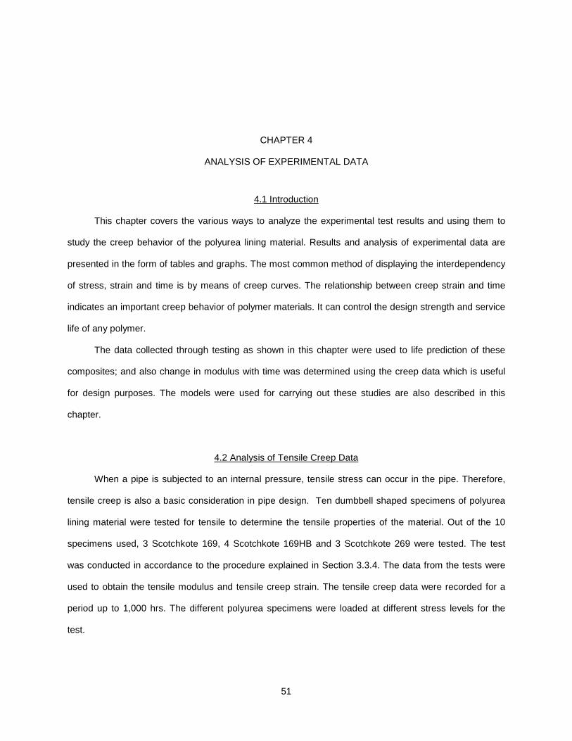
51
CHAPTER 4
ANALYSIS OF EXPERIMENTAL DATA
4.1 Introduction
This chapter covers the various ways to analyze the experimental test results and using them to
study the creep behavior of the polyurea lining material. Results and analysis of experimental data are
presented in the form of tables and graphs. The most common method of displaying the interdependency
of stress, strain and time is by means of creep curves. The relationship between creep strain and time
indicates an important creep behavior of polymer materials. It can control the design strength and service
life of any polymer.
The data collected through testing as shown in this chapter were used to life prediction of these
composites; and also change in modulus with time was determined using the creep data which is useful
for design purposes. The models were used for carrying out these studies are also described in this
chapter.
4.2 Analysis of Tensile Creep Data
When a pipe is subjected to an internal pressure, tensile stress can occur in the pipe. Therefore,
tensile creep is also a basic consideration in pipe design. Ten dumbbell shaped specimens of polyurea
lining material were tested for tensile to determine the tensile properties of the material. Out of the 10
specimens used, 3 Scotchkote 169, 4 Scotchkote 169HB and 3 Scotchkote 269 were tested. The test
was conducted in accordance to the procedure explained in Section 3.3.4. The data from the tests were
used to obtain the tensile modulus and tensile creep strain. The tensile creep data were recorded for a
period up to 1,000 hrs. The different polyurea specimens were loaded at different stress levels for the
test.

52
The maximum strain in the fibers due to elongation of the tensile creep test can be expressed in
terms of change in length by the original length of the specimen. Polyurea being a viscoelastic material
can attain high elongation levels before rupture occurs. Ultimate elongation is the property that defines
elastomeric materials. However, ultimate elongation still does not provide a precise indication of
serviceability because service conditions do not require the polyurea material to stretch to any significant
fraction of its ultimate elongation.
ASTM standard D2990 section 10.3 recommends the tensile stress should be such that it
produces 1% strain in 1,000 hours. In tensile tests, it is recommended that the strain be limited to 5% (i.e.
0.1319 in. (3.35 mm) elongation) if the specimen does not fail before reaching this strain level. Table 4.1
lists the various loads selected for the different polyurea composite specimens based on the trail test
carried out for 700 hours.
Table 4.1 - Load Selection for Various Polyurea Specimens
Polyurea Type Number of Specimens Loads (lbs)
169 3 1.5 1.5 1.75 -
169 HB 4 2 2.5 3 3.5
269 3 2 2 3 -
The following table summarizes the ratio of applied constant stress by corresponding strain.
Table 4.2 presents the stress values of various polyurea specimens along with their corresponding tensile
strain at various time intervals.
The creep test results are presented in Figures 4.1, 4.2 and 4.3 highlighting the effect of stress on
the response characteristic with time. The different graphs for creep strain data (%) versus time (hours)
for 169, 169HB and 269 specimens tested can be obtained using constitutive relationship. It can be seen
clearly that at higher stresses the failure is faster for all specimens.
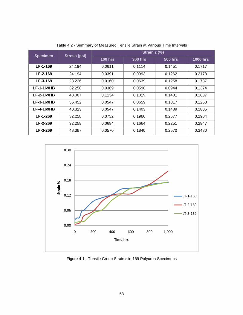
53
Table 4.2 - Summary of Measured Tensile Strain at Various Time Intervals
Specimen Stress (psi) Strain ε (%)
100 hrs 300 hrs 500 hrs 1000 hrs
LF-1-169 24.194 0.0611 0.1114 0.1451 0.1717
LF-2-169 24.194 0.0391 0.0993 0.1262 0.2178
LF-3-169 28.226 0.0160 0.0639 0.1258 0.1737
LF-1-169HB 32.258 0.0369 0.0590 0.0944 0.1374
LF-2-169HB 48.387 0.1134 0.1319 0.1431 0.1837
LF-3-169HB 56.452 0.0547 0.0659 0.1017 0.1258
LF-4-169HB 40.323 0.0547 0.1403 0.1439 0.1805
LF-1-269 32.258 0.0752 0.1966 0.2577 0.2904
LF-2-269 32.258 0.0694 0.1664 0.2251 0.2947
LF-3-269 48.387 0.0570 0.1840 0.2570 0.3430
Figure 4.1 - Tensile Creep Strain ε in 169 Polyurea Specimens
0.00
0.06
0.12
0.18
0.24
0.30
0 200 400 600 800 1,000
Str
ain
%
Time,hrs
LT-1-169
LT-2-169
LT-3-169

54
Based on Figures 4.1 & 4.2 all test specimens demonstrated a similar tensile behavior except for
specimen 269 in Figure 4.3. Specimen 269 showed significantly elongation and thus low creep modulus
than the other specimens.
Figure 4.2 - Tensile Creep Strain ε in 169HB Polyurea Specimens
Figure 4.3 - Tensile Creep Strain ε in 269 Polyurea Specimens
0
0.06
0.12
0.18
0.24
0 200 400 600 800 1,000
Str
ain
%
Time,hrs
LT-1-
169HB
LT-2-
169HB
LT-3-
169HB
0
0.1
0.2
0.3
0.4
0 200 400 600 800 1,000
Str
ain
%
Time,hrs
LT-1-269
LT-2-269
LT-3-269
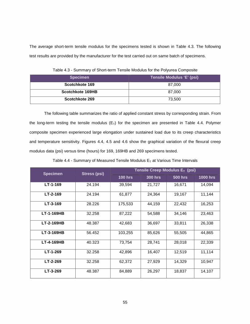
55
The average short-term tensile modulus for the specimens tested is shown in Table 4.3. The following
test results are provided by the manufacturer for the test carried out on same batch of specimens.
Table 4.3 - Summary of Short-term Tensile Modulus for the Polyurea Composite
Specimen Tensile Modulus ‘E’ (psi)
Scotchkote 169 87,000
Scotchkote 169HB 87,000
Scotchkote 269 73,500
The following table summarizes the ratio of applied constant stress by corresponding strain. From
the long-term testing the tensile modulus (ET) for the specimen are presented in Table 4.4. Polymer
composite specimen experienced large elongation under sustained load due to its creep characteristics
and temperature sensitivity. Figures 4.4, 4.5 and 4.6 show the graphical variation of the flexural creep
modulus data (psi) versus time (hours) for 169, 169HB and 269 specimens tested.
Table 4.4 - Summary of Measured Tensile Modulus ET at Various Time Intervals
Specimen Stress (psi) Tensile Creep Modulus E T (psi)
100 hrs 300 hrs 500 hrs 1000 hrs
LT-1-169 24.194 39,594 21,727 16,671 14,094
LT-2-169 24.194 61,877 24,364 19,167 11,144
LT-3-169 28.226 175,533 44,159 22,432 16,253
LT-1-169HB 32.258 87,222 54,588 34,146 23,463
LT-2-169HB 48.387 42,683 36,697 33,811 26,338
LT-3-169HB 56.452 103,255 85,626 55,505 44,865
LT-4-169HB 40.323 73,754 28,741 28,018 22,339
LT-1-269 32.258 42,896 16,407 12,519 11,114
LT-2-269 32.258 62,372 27,929 14,329 10,947
LT-3-269 48.387 84,889 26,297 18,837 14,107
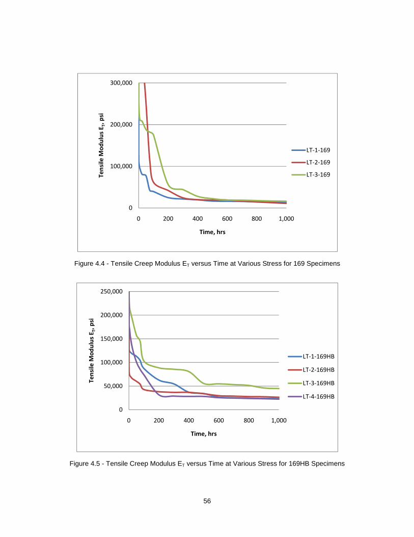
56
Figure 4.4 - Tensile Creep Modulus ET versus Time at Various Stress for 169 Specimens
Figure 4.5 - Tensile Creep Modulus ET versus Time at Various Stress for 169HB Specimens
0
100,000
200,000
300,000
0 200 400 600 800 1,000
Te
nsi
le M
od
ulu
s E
T,
psi
Time, hrs
LT-1-169
LT-2-169
LT-3-169
0
50,000
100,000
150,000
200,000
250,000
0 200 400 600 800 1,000
Te
nsi
le M
od
ulu
s E
T,
psi
Time, hrs
LT-1-169HB
LT-2-169HB
LT-3-169HB
LT-4-169HB
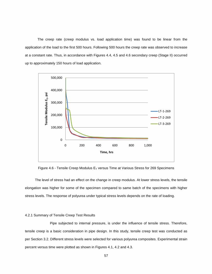
57
The creep rate (creep modulus vs. load application time) was found to be linear from the
application of the load to the first 500 hours. Following 500 hours the creep rate was observed to increase
at a constant rate. Thus, in accordance with Figures 4.4, 4.5 and 4.6 secondary creep (Stage II) occurred
up to approximately 150 hours of load application.
Figure 4.6 - Tensile Creep Modulus ET versus Time at Various Stress for 269 Specimens
The level of stress had an effect on the change in creep modulus. At lower stress levels, the tensile
elongation was higher for some of the specimen compared to same batch of the specimens with higher
stress levels. The response of polyurea under typical stress levels depends on the rate of loading.
4.2.1 Summary of Tensile Creep Test Results
Pipe subjected to internal pressure, is under the influence of tensile stress. Therefore,
tensile creep is a basic consideration in pipe design. In this study, tensile creep test was conducted as
per Section 3.2. Different stress levels were selected for various polyurea composites. Experimental strain
percent versus time were plotted as shown in Figures 4.1, 4.2 and 4.3.
0
100,000
200,000
300,000
400,000
500,000
0 200 400 600 800 1,000
Te
nsi
le M
od
ulu
s E
T,
psi
Time, hrs
LT-1-269
LT-2-269
LT-3-269
58
The average tensile strain for Polyurea 169 specimens after 1,000 hrs was found to be
approximately 0.002, for 169HB was 0.0015, whereas for 269 was 0.003. Similarly the tensile modulus
after 1,000 hours for 169 specimens was 13,830 psi, for 169HB was 29,250 psi and for 269 was 12,056
psi. In the linear creep range, the average tensile creep modulus for 169 specimens is about 34% of
short-term tensile modulus (87,000 psi), for 169HB is about 14% of short-term tensile modulus (87,000
psi) and for 269 specimens it is approximately 16 % of short-term tensile modulus (73,500 psi).
With reference to the above results, the creep strain rates decrease very rapidly at the initial
stage and further deforms slowly after 500 hours of loading during the tests. It can be concluded that
there is very little elongation for all the three composites and load needs to be increased to get
appropriate strain and elongation. Also the elongation needs to be monitored for more number of hours to
study their behavior.
4.3 Analysis of Flexural Creep Data
When a pipe begins to buckle, the pipe no longer keeps its shape in a circle, so the bending
moment which exists in the pipe increases. Therefore, bending is one of the typical factors which could
affect creep behavior of the pipe. Hence, it is necessary to investigate the viscoelastic behavior of the
pipe material under flexure.
Eight specimens of polyurea lining material were tested for flexural in longitudinal directions to
determine the flexural properties of the material. Three different composite of polyurea flexural specimens
169, 169HB and 269 were used for the test period up to 1,000 hrs. The different polyurea composite
specimens were loaded at different stress levels. The specimens 269 and 169 were tested for three
different loads, while the specimen 169HB was tested for two different loading conditions. The respective
strains and flexural modulus for these specimens were calculated and tabulated based on the equations
explained in Chapter 3.
Tests results were analyzed as per the ASTM D790 and ASTM D2990 specifications. The test
was conducted in accordance with the procedure explained in section 3.4.4. The data from the tests were
used to obtain the flexural modulus and flexural strength. Table 4.5 lists the various loads selected for the
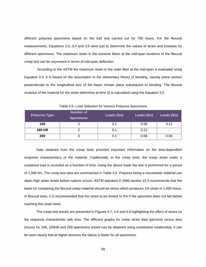
59
different polyurea specimens based on the trail test carried out for 700 hours. For the flexural
measurements, Equations 3.3, 3.4 and 3.5 were just to determine the values of strain and modulus for
different specimens. The maximum strain in the extreme fibers at the mid-span locations of the flexural
creep test can be expressed in terms of mid-span deflection.
According to the ASTM the maximum strain in the outer fiber at the mid-span is evaluated using
Equation 3.4. It is based on the assumption in the elementary theory of bending, namely plane section
perpendicular to the longitudinal axis of the beam remain plane subsequent to bending. The flexural
modulus of the material for the strain determine at time (t) is calculated using the Equation 3.5.
Table 4.5- Load Selection for Various Polyurea Specimens
Polyurea Type Number of
Specimens Loads (lbs) Loads (lbs) Loads (lbs)
169 3 0.1 0.08 0.12
169 HB 2 0.1 0.12 -
269 3 0.1 0.08 0.06
Data obtained from the creep tests provided important information on the time-dependent
response characteristics of the material. Traditionally, in the creep tests, the creep strain under a
sustained load is recorded as a function of time. Using the above loads the test is performed for a period
of 1,000 hrs. The creep test data are summarized in Table 4.6. Polyurea being a viscoelastic material can
attain high strain levels before rupture occurs. ASTM standard D 2990 section 10.3 recommends that the
basis for comparing the flexural creep material should be stress which produces 1% strain in 1,000 hours.
In flexural tests, it is recommended that the strain to be limited to 5% if the specimen does not fail before
reaching this strain level.
The creep test results are presented in Figures 4.7, 4.8 and 4.9 highlighting the effect of stress on
the response characteristic with time. The different graphs for creep strain data (percent) versus time
(hours) for 169, 169HB and 269 specimens tested can be obtained using constitutive relationship. It can
be seen clearly that at higher stresses the failure is faster for all specimens.

60
Table 4.6 - Summary of Measured Flexural Strain at Various Time Intervals
Specimen Stress (psi) Strain ε (%)
100 hrs 300 hrs 500 hrs 1000 hrs
LF-1-169 33.871 0.070 0.100 0.130 0.160
LF-2-169 27.097 0.069 0.111 0.136 0.148
LF-3-169 40.645 0.088 0.145 0.176 0.193
LF-1-169HB 33.871 0.263 0.428 0.685 0.996
LF-2-169HB 40.645 0.201 0.400 0.534 0.652
LF-1-269 33.871 1.240 2.790 4.210 5.625
LF-2-269 27.097 1.350 1.588 2.258 3.444
LF-3-269 20.323 0.819 1.852 2.890 3.980
Figure 4.7 – Flexural Creep Strain ε in 169 Polyurea Specimens
Using Equation 3.4, the maximum strain in the extreme fibers at the mid-span location of the
flexural tests specimens was calculated based on the deflection obtained. The directly proportional
relationship implies that the conclusions drawn earlier for deflection are also applicable for strain.
However, it is important to take a look at the strain values in this case because they are used to define
the flexural modulus of the polyurea composite. From the Figures 4.7 and 4.8 it is concluded that the
0
0.05
0.1
0.15
0.2
0.25
0 200 400 600 800 1000
Str
ain
, %
Time, hrs
LF-1-169
LF-2-169
LF-3-169

61
strain is within the limit of 1% in 1, 000 hours of the test. However, the stress in 169 specimens can be
increased to obtain the more specific results as per the ASTM.
Figure 4.8 - Flexural Creep Strain ε in 169HB Polyurea Specimens
Figure 4.9 - Flexural Creep Strain ε in 269 Polyurea Specimens
0
0.2
0.4
0.6
0.8
1
1.2
0 200 400 600 800 1000
Str
ain
, %
Time, hrs
LF-1-169HB
LF-2-169HB
0
1
2
3
4
5
6
0 200 400 600 800 1000
Str
ain
, %
Time, hrs
LF-1-269
LF-2-269
LF-3-269
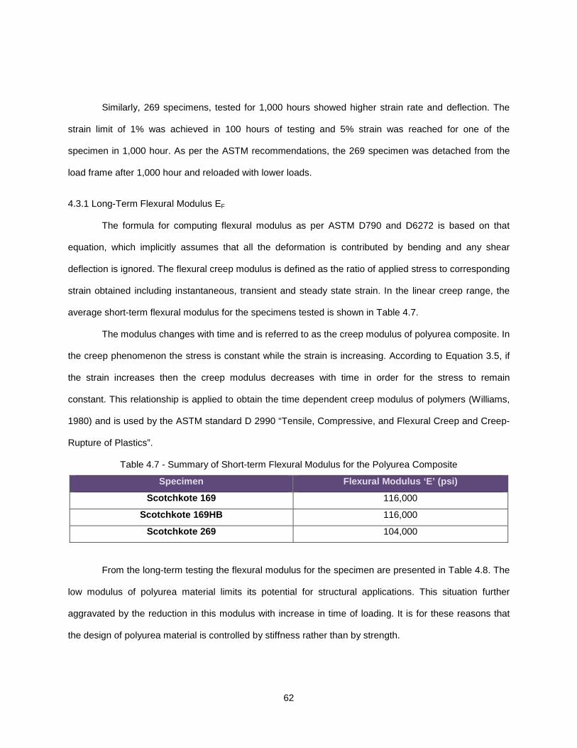
62
Similarly, 269 specimens, tested for 1,000 hours showed higher strain rate and deflection. The
strain limit of 1% was achieved in 100 hours of testing and 5% strain was reached for one of the
specimen in 1,000 hour. As per the ASTM recommendations, the 269 specimen was detached from the
load frame after 1,000 hour and reloaded with lower loads.
4.3.1 Long-Term Flexural Modulus EF
The formula for computing flexural modulus as per ASTM D790 and D6272 is based on that
equation, which implicitly assumes that all the deformation is contributed by bending and any shear
deflection is ignored. The flexural creep modulus is defined as the ratio of applied stress to corresponding
strain obtained including instantaneous, transient and steady state strain. In the linear creep range, the
average short-term flexural modulus for the specimens tested is shown in Table 4.7.
The modulus changes with time and is referred to as the creep modulus of polyurea composite. In
the creep phenomenon the stress is constant while the strain is increasing. According to Equation 3.5, if
the strain increases then the creep modulus decreases with time in order for the stress to remain
constant. This relationship is applied to obtain the time dependent creep modulus of polymers (Williams,
1980) and is used by the ASTM standard D 2990 “Tensile, Compressive, and Flexural Creep and Creep-
Rupture of Plastics”.
Table 4.7 - Summary of Short-term Flexural Modulus for the Polyurea Composite
Specimen Flexural Modulus ‘E’ (psi)
Scotchkote 169 116,000
Scotchkote 169HB 116,000
Scotchkote 269 104,000
From the long-term testing the flexural modulus for the specimen are presented in Table 4.8. The
low modulus of polyurea material limits its potential for structural applications. This situation further
aggravated by the reduction in this modulus with increase in time of loading. It is for these reasons that
the design of polyurea material is controlled by stiffness rather than by strength.
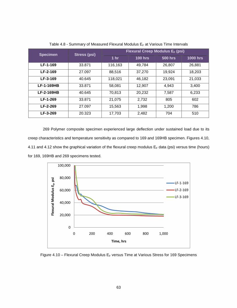
63
Table 4.8 - Summary of Measured Flexural Modulus EF at Various Time Intervals
Specimen Stress (psi) Flexural Creep Modulus E F (psi)
1 hr 100 hrs 500 hrs 1000 hrs
LF-1-169 33.871 116,163 49,784 26,807 26,881
LF-2-169 27.097 88,516 37,270 19,924 18,203
LF-3-169 40.645 118,021 46,182 23,091 21,033
LF-1-169HB 33.871 58,081 12,907 4,943 3,400
LF-2-169HB 40.645 70,813 20,232 7,587 6,233
LF-1-269 33.871 21,075 2,732 805 602
LF-2-269 27.097 15,563 1,998 1,200 786
LF-3-269 20.323 17,703 2,482 704 510
269 Polymer composite specimen experienced large deflection under sustained load due to its
creep characteristics and temperature sensitivity as compared to 169 and 169HB specimen. Figures 4.10,
4.11 and 4.12 show the graphical variation of the flexural creep modulus EF data (psi) versus time (hours)
for 169, 169HB and 269 specimens tested.
Figure 4.10 – Flexural Creep Modulus EF versus Time at Various Stress for 169 Specimens
0
20,000
40,000
60,000
80,000
100,000
0 200 400 600 800 1,000
Fle
xu
ral
Mo
du
lus
EF,
psi
Time, hrs
LF-1-169
LF-2-169
LF-3-169
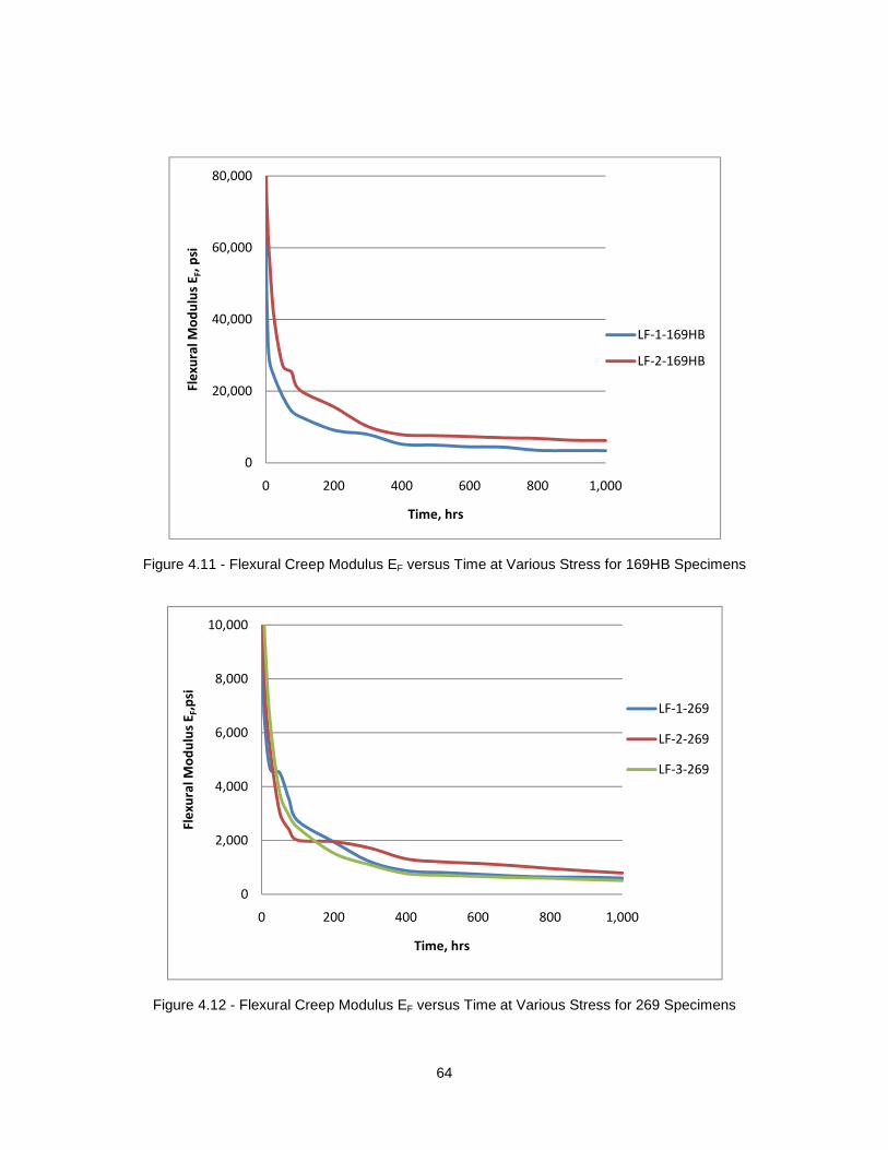
64
Figure 4.11 - Flexural Creep Modulus EF versus Time at Various Stress for 169HB Specimens
Figure 4.12 - Flexural Creep Modulus EF versus Time at Various Stress for 269 Specimens
0
20,000
40,000
60,000
80,000
0 200 400 600 800 1,000
Fle
xu
ral
Mo
du
lus
EF,
psi
Time, hrs
LF-1-169HB
LF-2-169HB
0
2,000
4,000
6,000
8,000
10,000
0 200 400 600 800 1,000
Fle
xu
ral
Mo
du
lus
EF,p
si
Time, hrs
LF-1-269
LF-2-269
LF-3-269
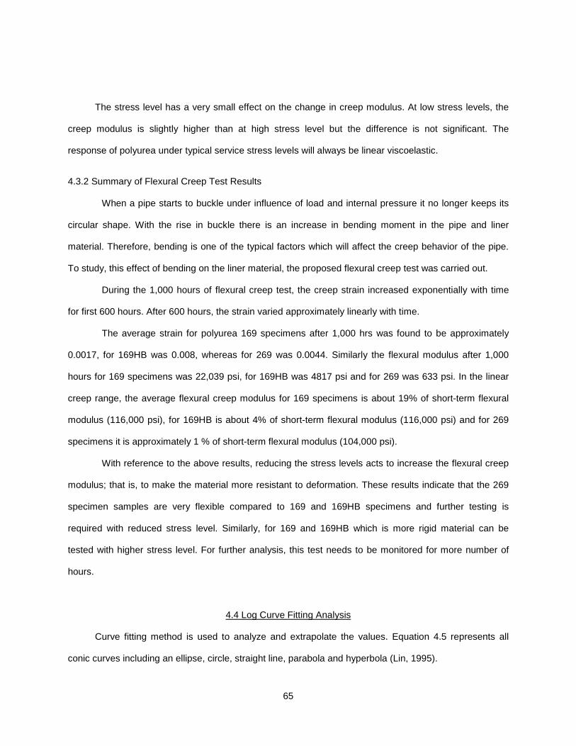
65
The stress level has a very small effect on the change in creep modulus. At low stress levels, the
creep modulus is slightly higher than at high stress level but the difference is not significant. The
response of polyurea under typical service stress levels will always be linear viscoelastic.
4.3.2 Summary of Flexural Creep Test Results
When a pipe starts to buckle under influence of load and internal pressure it no longer keeps its
circular shape. With the rise in buckle there is an increase in bending moment in the pipe and liner
material. Therefore, bending is one of the typical factors which will affect the creep behavior of the pipe.
To study, this effect of bending on the liner material, the proposed flexural creep test was carried out.
During the 1,000 hours of flexural creep test, the creep strain increased exponentially with time
for first 600 hours. After 600 hours, the strain varied approximately linearly with time.
The average strain for polyurea 169 specimens after 1,000 hrs was found to be approximately
0.0017, for 169HB was 0.008, whereas for 269 was 0.0044. Similarly the flexural modulus after 1,000
hours for 169 specimens was 22,039 psi, for 169HB was 4817 psi and for 269 was 633 psi. In the linear
creep range, the average flexural creep modulus for 169 specimens is about 19% of short-term flexural
modulus (116,000 psi), for 169HB is about 4% of short-term flexural modulus (116,000 psi) and for 269
specimens it is approximately 1 % of short-term flexural modulus (104,000 psi).
With reference to the above results, reducing the stress levels acts to increase the flexural creep
modulus; that is, to make the material more resistant to deformation. These results indicate that the 269
specimen samples are very flexible compared to 169 and 169HB specimens and further testing is
required with reduced stress level. Similarly, for 169 and 169HB which is more rigid material can be
tested with higher stress level. For further analysis, this test needs to be monitored for more number of
hours.
4.4 Log Curve Fitting Analysis
Curve fitting method is used to analyze and extrapolate the values. Equation 4.5 represents all
conic curves including an ellipse, circle, straight line, parabola and hyperbola (Lin, 1995).

66
2 2y A x B x C= + + Equation 4.5
For most of the polymer materials, the long-term performance the design life can be quite long
period. The log-log method is used to predict the design life of the material which will tend to display
linearly on the log-log coordinate. Considering x and y coordinates as log.
Therefore, y = Log ε
and x = Log t
Hence, Equation 4.5 becomes
Equation 4.6
Where,
ε = Creep Strain at a Constant Stress
t = Time, in Hours,
A, B, C = Coefficient (Stress, Material, loading condition related)
Since ε, is less than 1, a negative solution of the Equation 4.6 is selected (Lin, 1995).
Equation 4.7
The coefficient of the equation is determined using the following procedure. Three points of test
are selected for each stress, choosing the beginning of the test as t1, t2 =1.0 hr and end of the test t3. In
this study t1 = 0.0167 hr, t2 = 1 hr and t3 = 500 hrs. Since analysis is based on 1000 hrs, which is
insufficient to predict 50-year design life of this material.
When t = 1 hr Equation 4.6 becomes;
Equation 4.8
Substituting the value of t1, t3 and ε t1 and ε t3 into Equation 4.6, we get.
[ ] [ ]2 2( ) ( ) log( )Log A Log t B t Cε = + +
[ ]2( ) ( ) log( )Log A Log t B t Cε = − + +
21(log( ))tC ε ==

67
Equation 4.9
Equation 4.10
Where,
εt1, εt3 = Creep strain at time t1 and t3, respectively.
4.4.1 Log Curve Fitting Analysis for Flexural Specimens
Coefficients of Equation 4.6 for Flexural Creep experiment were obtained using the above method.
Table 4.9 shows the coefficient for the flexural experiment using the curve fitting method.
Table 4.9 – Coefficients for Flexural Creep using Log-Curve Fitting Method
Specimen Stress, psi Coefficient
A B C
LF-1-169 33.871 -0.45027 -0.80026 13.8476
LF-2-169 27.097 -0.04829 -1.38653 12.3105
LF-3-169 40.645 -0.21616 -1.06295 12.0306
LF-1-269 33.871 0.24689 -2.86141 7.81694
LF-1-169HB 33.871 -0.22302 -1.54376 10.4754
LF-2-169HB 40.645 0.07080 -2.17988 10.5243
LF-2-269 27.097 0.07018 -2.00654 7.61456
LF-3-269 20.323 -0.17155 -1.85949 8.63949
Because of the limited time for observation, the coefficients in equation 4.6 were obtained based
on only 500 hours of data. The equation should not be used to predict the creep behavior for more than
single decade at the end of the experimental data. Table 4.10 lists the measured bending creep strain by
curve fitting method at various times comparing it with the long-term flexural experimental values.
[ ] [ ]2 2
1 1 1( ) ( ) log( )tLog A Log t B t Cε = + +
[ ] [ ]2 2
3 3 3( ) ( ) log( )tLog A Log t B t Cε = + +

68
Table 4.10 – Comparison of Experimental and Theoretical Flexural Strain %
Specimen Stress,
psi
Experimental ε (%) Theoretical ε (%)
(Log Curve Fitting Method)
500
hrs
1000
hrs
3000
hrs
1000
0 hrs
500
hrs
1000
hrs
3000
hrs
10000
hrs
LF-1-169 33.871 0.126 0.160 - - 0.126 0.190 0.425 1.395
LF-2-169 27.097 0.136 0.148 - - 0.136 0.166 0.235 0.356
LF-3-169 40.645 0.176 0.193 - - 0.176 0.236 0.405 0.834
LF-1-169HB 33.871 0.685 0.996 - - 0.685 1.099 1.800 2.945
LF-2-169HB 40.645 0.536 0.652 - - 0.536 0.708 1.123 1.932
LF-1-269 33.871 4.210 5.625 - - 4.210 6.220 11.930 27.091*
LF-2-269 27.097 2.258 3.444 - - 2.258 3.219 6.0385 14.341*
LF-3-269 20.323 2.890 3.980 - - 2.885 5.865 48.329 -
Note: * Data extrapolated is beyond the limit of the test results. As per ASTM requirements the maximum strain generated in the specimen should not be more than 5%.
4.4.2 Log Curve Fitting Analysis for Tensile Specimens
Similarly, coefficients of Equation 4.6 for tensile creep experiment were obtained using the above
method. Table 4.11 shows the coefficient for the tensile experiment using log curve fitting method.
Table 4.11 - Coefficients for Tensile Creep using Log Curve Fitting Method
Specimen Stress, psi Coefficient
A B C
LT-1-169 24.194 0.0329475 -2.1216924 13.54132
LT-2-169 24.194 -0.06723859 -3.8643536 19.32283
LT-3-169 28.226 -0.4500371 -1.4925315 15.71778
LT-2-169HB 48.387 0.25724330 -1.5584223 10.42312
LT-4-169HB 40.323 0.26643243 -2.6775276 13.63203
LT-1-269 32.258 0.06068314 -3.9601995 16.94892
LT-2-269 32.258 -0.66137137 -1.6180853 15.84744
LT-3-269 48.387 0.02424393 -2.8446675 14.15419

69
Also for the tensile test because of the limited time for observation, the coefficients in equation
4.9 were obtained based on only 500 hours of data. Table 4.12 lists the measured bending creep strain
by curve fitting method at various times comparing it with the long-term flexural experimental values.
Table 4.12 - Comparison of Experimental and Theoretical Tensile Strain %
Specimen Stress,
psi
Experimental ε (%) Theoretical ε (%)
(Log Curve Fitting Method)
500
hrs
1000
hrs
3000
hrs
10000
hrs
500
hrs
1000
hrs
3000
hrs
10000
hrs
LT-1-169 24.194 0.1451 0.1717 - - 0.1451 0.1846 0.2743 0.4339
LT-2-169 24.194 0.1262 0.2173 - - 0.1262 0.2141 0.5593 2.1369
LT-3-169 28.226 0.1258 0.1736 - - 0.1258 0.2082 0.5553 2.5354
LT-2-169HB 48.387 0.1431 0.1837 - - 0.1430 0.1446 0.1417 0.1612
LT-4-169HB 40.323 0.1439 0.1805 0.1291 0.1486 0.1792 0.2087
LT-1-269 32.258 0.2578 0.2902 - - 0.2576 0.4270 1.0519 3.6149
LT-2-269 32.258 0.2251 0.2947 - - 0.2623 0.6861 3.2238 -
LT-3-269 48.387 0.2568 0.3430 - - 0.2634 0.3834 0.7336 1.6649
Comparing the strain values obtained from curve fitting method with that of the experimental data,
it was found that both the results were close. Using curve fitting method is not suitable for predicting the
strain value for more than a decade. Since 1,000 hours is just a small part of the service life, so the real
slope of the creep cannot be determined with very short-term data. Therefore, Equation 4.6 will not
accurately predict the creep behavior of material more than 10,000 hours if the data observed is not
adequate.
4.5 Findley’s Power Law Model
One of the ways of describing the time-dependent behavior of polymer in linear and moderately
non-linear regions is use of Findley’s constants. Findley’s employed equation of the type (Findley, 1989):
Equation 4.11
( ) s inh sinhn
o to o
t tσ σ
ε ε εσ σ
= +
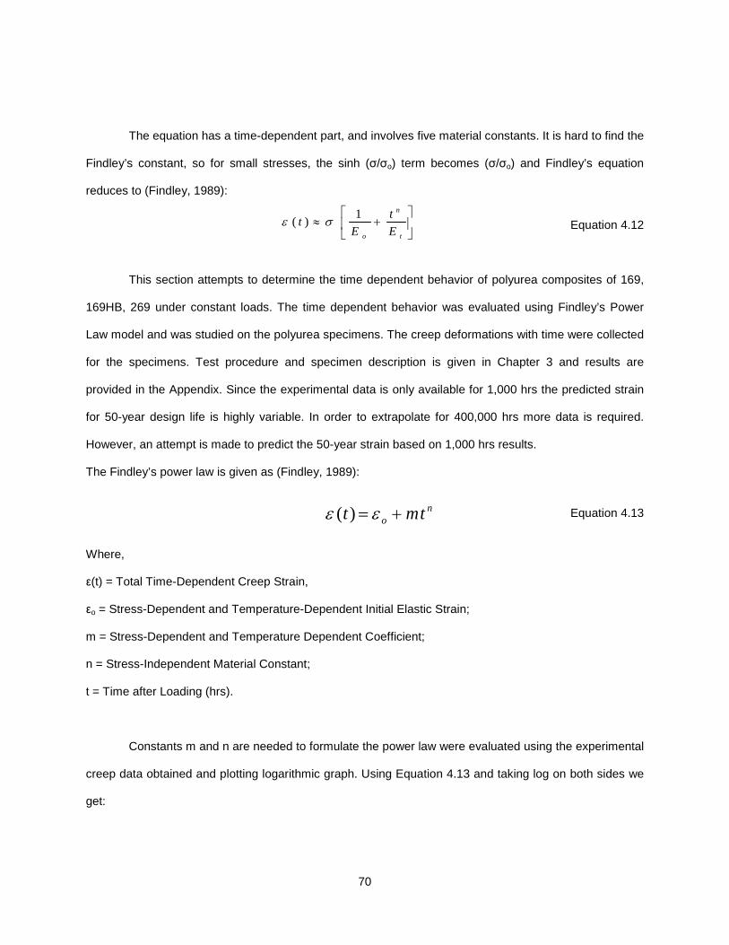
70
The equation has a time-dependent part, and involves five material constants. It is hard to find the
Findley’s constant, so for small stresses, the sinh (σ/σo) term becomes (σ/σo) and Findley’s equation
reduces to (Findley, 1989):
Equation 4.12
This section attempts to determine the time dependent behavior of polyurea composites of 169,
169HB, 269 under constant loads. The time dependent behavior was evaluated using Findley’s Power
Law model and was studied on the polyurea specimens. The creep deformations with time were collected
for the specimens. Test procedure and specimen description is given in Chapter 3 and results are
provided in the Appendix. Since the experimental data is only available for 1,000 hrs the predicted strain
for 50-year design life is highly variable. In order to extrapolate for 400,000 hrs more data is required.
However, an attempt is made to predict the 50-year strain based on 1,000 hrs results.
The Findley’s power law is given as (Findley, 1989):
Equation 4.13
Where,
ε(t) = Total Time-Dependent Creep Strain,
εo = Stress-Dependent and Temperature-Dependent Initial Elastic Strain;
m = Stress-Dependent and Temperature Dependent Coefficient;
n = Stress-Independent Material Constant;
t = Time after Loading (hrs).
Constants m and n are needed to formulate the power law were evaluated using the experimental
creep data obtained and plotting logarithmic graph. Using Equation 4.13 and taking log on both sides we
get:
1( )
n
o t
tt
E Eε σ
≈ +
( ) not mtε ε= +
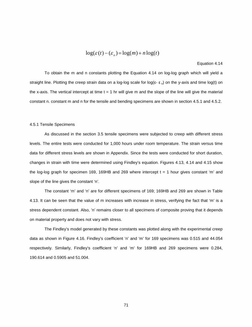
71
log( ( ) ( ) log( ) log( )ot m n tε ε− = +
Equation 4.14
To obtain the m and n constants plotting the Equation 4.14 on log-log graph which will yield a
straight line. Plotting the creep strain data on a log-log scale for log(ε- ε o) on the y-axis and time log(t) on
the x-axis. The vertical intercept at time t = 1 hr will give m and the slope of the line will give the material
constant n. constant m and n for the tensile and bending specimens are shown in section 4.5.1 and 4.5.2.
4.5.1 Tensile Specimens
As discussed in the section 3.5 tensile specimens were subjected to creep with different stress
levels. The entire tests were conducted for 1,000 hours under room temperature. The strain versus time
data for different stress levels are shown in Appendix. Since the tests were conducted for short duration,
changes in strain with time were determined using Findley’s equation. Figures 4.13, 4.14 and 4.15 show
the log-log graph for specimen 169, 169HB and 269 where intercept t = 1 hour gives constant ‘m’ and
slope of the line gives the constant ‘n’.
The constant ‘m’ and ‘n’ are for different specimens of 169; 169HB and 269 are shown in Table
4.13. It can be seen that the value of m increases with increase in stress, verifying the fact that ‘m’ is a
stress dependent constant. Also, ’n’ remains closer to all specimens of composite proving that it depends
on material property and does not vary with stress.
The Findley’s model generated by these constants was plotted along with the experimental creep
data as shown in Figure 4.16. Findley’s coefficient ‘n’ and ‘m’ for 169 specimens was 0.515 and 44.054
respectively. Similarly, Findley’s coefficient ‘n’ and ‘m’ for 169HB and 269 specimens were 0.284,
190.614 and 0.5905 and 51.004.

72
Figure 4.13 - Log-Log Plot of Specimen 169 to Evaluate Findley’s Constant
Figure 4.14 - Log-Log Plot of Specimen 169HB to Evaluate Findley’s Constant
0
500
1000
1500
2000
2500
0 200 400 600 800 1000 1200
(et-
e0
) m
icro
stri
an
Time hrs
LT-1-169
LT-2-169
LT-3-169
PREDICTED
0
200
400
600
800
1000
1200
1400
1600
1800
2000
0 200 400 600 800 1000 1200
(et-
eo
) m
icro
stra
in
Time hrs
LT-1-169HB
LT-2-169HB
LT-3-169HB
LT-4-169HB
PREDICTED
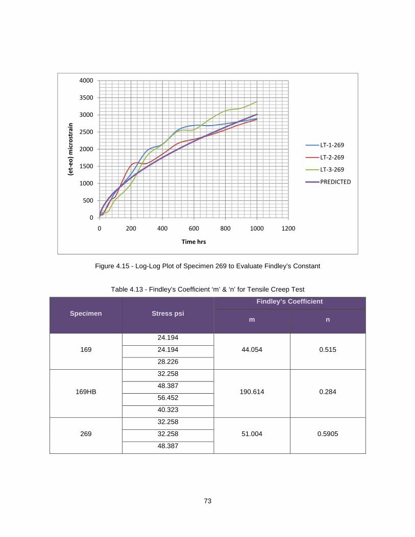
73
Figure 4.15 - Log-Log Plot of Specimen 269 to Evaluate Findley’s Constant
Table 4.13 - Findley’s Coefficient ‘m’ & ‘n’ for Tensile Creep Test
Specimen Stress psi
Findley’s Coefficient
m n
169
24.194
44.054 0.515 24.194
28.226
169HB
32.258
190.614 0.284 48.387
56.452
40.323
269
32.258
51.004 0.5905 32.258
48.387
0
500
1000
1500
2000
2500
3000
3500
4000
0 200 400 600 800 1000 1200
(et-
eo
) m
icro
stra
in
Time hrs
LT-1-269
LT-2-269
LT-3-269
PREDICTED
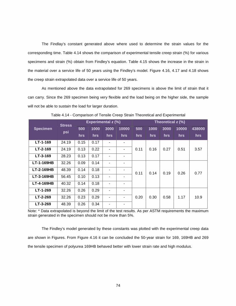
74
The Findlay’s constant generated above where used to determine the strain values for the
corresponding time. Table 4.14 shows the comparison of experimental tensile creep strain (%) for various
specimens and strain (%) obtain from Findley’s equation. Table 4.15 shows the increase in the strain in
the material over a service life of 50 years using the Findley’s model. Figure 4.16, 4.17 and 4.18 shows
the creep strain extrapolated data over a service life of 50 years.
As mentioned above the data extrapolated for 269 specimens is above the limit of strain that it
can carry. Since the 269 specimen being very flexible and the load being on the higher side, the sample
will not be able to sustain the load for larger duration.
Table 4.14 - Comparison of Tensile Creep Strain Theoretical and Experimental
Specimen Stress
psi
Experimental ε (%) Theoretical ε (%)
500
hrs
1000
hrs
3000
hrs
10000
hrs
500
hrs
1000
hrs
3000
hrs
10000
hrs
438000
hrs
LT-1-169 24.19 0.15 0.17 - -
0.11 0.16 0.27 0.51 3.57 LT-2-169 24.19 0.13 0.22 - -
LT-3-169 28.23 0.13 0.17 - -
LT-1-169HB 32.26 0.09 0.14 - -
0.11 0.14 0.19 0.26 0.77 LT-2-169HB 48.39 0.14 0.18 - -
LT-3-169HB 56.45 0.10 0.13 - -
LT-4-169HB 40.32 0.14 0.18 - -
LT-1-269 32.26 0.26 0.29 - -
0.20 0.30 0.58 1.17 10.9 LT-2-269 32.26 0.23 0.29 - -
LT-3-269 48.39 0.26 0.34 - -
Note: * Data extrapolated is beyond the limit of the test results. As per ASTM requirements the maximum strain generated in the specimen should not be more than 5%.
The Findley’s model generated by these constants was plotted with the experimental creep data
are shown in Figures. From Figure 4.16 it can be concluded the 50-year strain for 169, 169HB and 269
the tensile specimen of polyurea 169HB behaved better with lower strain rate and high modulus.

75
Figure 4.16 - Tensile Strain Prediction for 169, 169HB & 269 Specimens over 50-Year (Findley’s Law)
4.5.2 Flexural Specimens
As discussed in the section 3.4 flexural specimens were subjected to creep with different stress
levels. The entire tests were conducted for 1,000 hours under room temperature. The strain versus time
data for different stress levels are shown in Appendix. Since the tests were conducted for short duration,
changes in creep strain response for 50 years were extrapolated using Findley’s Power Law model.
Figures 4.17, 4.18 and 4.19 show the log-log graph for specimen 169, 169HB and 269 where intercept t =
1 hour gives constant m and slope of the line gives the constant ‘n.
The constant m and n are for different specimens of 169, 169HB and 269 are shown in Table
4.15. It can be seen that the value of ‘m’ increases with increase in stress, verifying the fact that ‘m’ is a
stress dependent constant. Also, an ‘n’ remains closer to all specimens of composite proving that ‘n’
depends on material property and does not vary with stress.
0.0
2.4
4.8
7.2
9.6
12.0
14.4
0 100000 200000 300000 400000 500000
Str
ain
%
Time, hrs
169 Specimen 169HB Specimen 269 Specimen
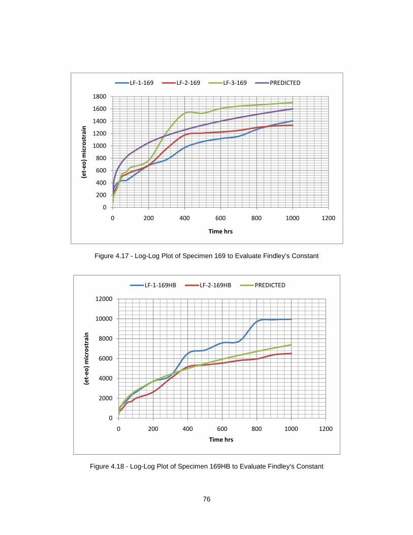
76
Figure 4.17 - Log-Log Plot of Specimen 169 to Evaluate Findley’s Constant
Figure 4.18 - Log-Log Plot of Specimen 169HB to Evaluate Findley’s Constant
0
200
400
600
800
1000
1200
1400
1600
1800
0 200 400 600 800 1000 1200
(et-
eo
) m
icro
stra
in
Time hrs
LF-1-169 LF-2-169 LF-3-169 PREDICTED
0
2000
4000
6000
8000
10000
12000
0 200 400 600 800 1000 1200
(et-
eo
) m
icro
stra
in
Time hrs
LF-1-169HB LF-2-169HB PREDICTED

77
Figure 4.19 - Log-Log Plot of Specimen 269 to Evaluate Findley’s Constant
Table 4.15 - Findley’s Coefficient ‘m’ & ‘n’ for Tensile Creep Test
Specimen Stress
psi
Findley’s Coefficient
m n
169
24.194
44.054 0.515 24.194
28.226
169HB
32.258
386.459 0.427 48.387
56.452
40.323
269
32.258
1164.045 0.509 32.258
48.387
The Findlay’s constant generated above where used to determine the strain values for the
corresponding time. Table 4.16 shows the comparison of experimental flexural creep strain (%) for
0
10000
20000
30000
40000
50000
60000
0 200 400 600 800 1000 1200
(et-
eo
) m
icro
stra
in
Time hrs
LF-1-269 LF-2-269 LF-3-269 PREDICTED

78
various specimens and strain (%) obtain from Findley’s equation. The Findley’s model generated by these
constant were plotted with the experimental data. Findley’s power law model proved to be a good
approximation of linear creep behavior of polyurea composite. Hence, Findley’s power law can be
successfully used to model creep for lower stress levels, since the tertiary creep stage approaches in
case of high stress levels.
Findley’s law does not predict the tertiary creep region, i.e. the time to failure that will occur in the
region. However, the law predicts the secondary creep region well. Figures 4.20 shows the creep strain
extrapolated data for 169, 169HB and 269 using Findley’s Power Law model for a service life of 50 years.
The data extrapolated for 269 specimens is above the limit of strain that it can carry. Since the 269
specimen being very flexible and the load being on the higher side, the sample will not be able to sustain
the load for larger duration.
Table 4.16 - Comparison of Flexural Creep Strain Theoretical and Experimental
Specimen Stress
psi
Experimental ε (%) Theoretical ε (%)
500
hrs
1000
hrs
3000
hrs
10000
hrs
500
hrs
1000
hrs
3000
hrs
10000
hrs
438000
hrs
LF-1-169 33.87 0.13 0.16 - -
0.13 0.16 0.21 0.29 0.78 LF-2-169 27.08 0.14 0.15 - -
LF-3-169 40.65 0.18 0.19 - -
LF-1-169HB 33.87 0.69 0.99 - - 0.55 0.74 1.18 1.98 9.94
LF-2-169HB 40.65 0.54 0.65 - -
LF-1-269 33.87 4.21 5.63 - -
2.76 3.93 6.87 12.69 - LF-2-269 27.08 2.26 3.44 - -
LF-3-269 20.32 2.89 3.98 - -
Note: * Data extrapolated is beyond the limit of the test results. As per ASTM requirements the maximum strain generated in the specimen should not be more than 5%.
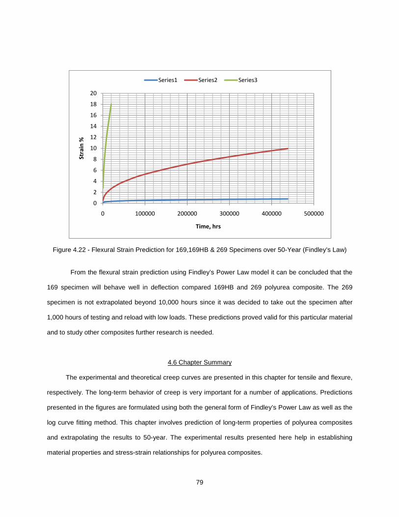
79
Figure 4.22 - Flexural Strain Prediction for 169,169HB & 269 Specimens over 50-Year (Findley’s Law)
From the flexural strain prediction using Findley’s Power Law model it can be concluded that the
169 specimen will behave well in deflection compared 169HB and 269 polyurea composite. The 269
specimen is not extrapolated beyond 10,000 hours since it was decided to take out the specimen after
1,000 hours of testing and reload with low loads. These predictions proved valid for this particular material
and to study other composites further research is needed.
4.6 Chapter Summary
The experimental and theoretical creep curves are presented in this chapter for tensile and flexure,
respectively. The long-term behavior of creep is very important for a number of applications. Predictions
presented in the figures are formulated using both the general form of Findley’s Power Law as well as the
log curve fitting method. This chapter involves prediction of long-term properties of polyurea composites
and extrapolating the results to 50-year. The experimental results presented here help in establishing
material properties and stress-strain relationships for polyurea composites.
0
2
4
6
8
10
12
14
16
18
20
0 100000 200000 300000 400000 500000
Str
ain
%
Time, hrs
Series1 Series2 Series3
80
CHAPTER 5
CONCLUSIONS AND RECOMMENDATIONS
5.1 Conclusions
This study developed an understanding of long-term test behavior of polyurea pipe lining used for
renewal of deteriorated potable water pipes. The liner materials used for testing are commercially
available composites of polyurea i.e. Scotchkote 169, 169HB and 269 used in pipe lining applications.
For this study, it was necessary to adopt an iterative approach to determine the loads that will
best represent the creep response over 10,000 hours of testing. In general, the creep testing provided
valuable information about the durability of the Scotchkote 169, 169HB and 269 lining. The long-term
tests conducted in this thesis, showed that the obtained creep data were in good agreement with
Findley’s Power law and log-fit method. These methods were used to analyze and extrapolate the creep
behavior and strain response of polyurea composite. It was observed that polyurea samples, loaded for
same period under similar loading conditions and stress, did not perform identical results. There were
differences observed both in strain, magnitude of deflection and elongation. This can be attributed to
material composition and stress distribution.
The results of creep behavior under different loading conditions for both tensile and flexure are
presented in the appendices. Based on the experimental results and theoretical studies, the following
conclusions are made:
Flexural Creep
Based on the 1,000 hours on polyurea composite specimens at room temperature, we can
conclude that 169 and 169HB polyurea specimens performed better in bending when compared to 269
specimens. This is due to more rigidity in case of 169 & 169HB specimen which provided a better stress
distribution. There was a 90% reduction in strength for 269 specimens, unlike the other two composites.
81
This concludes 269 polyurea to be more flexible material and 169 and 169HB more rigid. The value of
elastic modulus of the materials obtained from long-term test was compared with the values obtained
from the short-term tests results.
Tensile Creep
Polyurea composite specimens of dumbbell shape were used for evaluating the tensile and creep
properties. The 169, 169HB and 269 specimens, all performed well in tensile under constant stress and at
a constant room temperature. The average tensile modulus ET was very low compared to the short-term
modulus of the specimen.
Log-Curve Fitting
The log curve fitting method was in excellent conformity with the experimental data. Log curve
fitting also proved to be good practice to extrapolate the data up to 10,000 hours. Since the available
experimental data were for short duration, data extrapolation was not done for more than 10,000 hours.
Findley’s Power Law
The equation of Findley was used to predict the creep strain under tensile and flexure. The
results of the experiments were in agreement with the predicted values by this method. Using Findley’s
method to predict the 50-year data was also useful in determining the specimen that reached the 5%
strain limit. Using Findley’s Power Law model, stress-independent model, time-dependent strain was
predicted with accuracies that were acceptable. An important restriction to this model is that it cannot
describe non-linear tertiary creep; therefore stress levels must be kept sufficiently low to avoid this stage
of creep.
5.2 Limitations
Some of the limitations of this research are:
1. These tests are carried out in room temperature, but generally creep tests are usually conducted
at constant and lower temperatures.
2. The humidity was not maintained constant, where in actual cases the humidity is as low as 25%.
3. The loads selected for some of the specimens were too high which resulted in high strain rate.
4. Analysis is based on 1000 hrs, which is insufficient to predict 50-year design life of this material.
82
5.2 Recommendations for Future Research
Based on this study, the following recommendations for future research are being made:
1. Investigating the creep response at various temperatures such as below 70oF (21oC) and above
100oF (37oC). This will be useful in understanding the material behavior at extreme temperatures
and site conditions present in certain regions of the country
2. Investigating the creep behavior of the same specimen for longer duration of time
3. Conducting test by lowering and rising stress levels, than the ones used in this research to obtain
better creep curves
4. Comparing the creep response of polyurea composites under effect of temperature and moisture
5. Conducting other tests like stress relaxation and hydrostatic these specimens for further
understanding of the material properties
6. Developing standard short-term testing procedures with same samples and predicting the long-
term behavior using the results of the short-term tests.

83
APPENDIX A
TENSILE CREEP STRAIN DATA

84
A.1 Tensile Creep Strain Data – Polyurea 169 Specimen, @ Stress 24.19 psi
Creep of Polyurea 169 Tensile Loading at Room Tempe rature
Specimen = LT-1-169
Load, lbs = 1.50
Stress, psi = 24.19
Duration = 1000 hrs
Date Time (hrs) Temperature oF Elongation (mm) Strain % Strain
20-Jan-10 0.0167 71 0.004 0.0000671 0.0067
20-Jan-10 1 71 0.014 0.0002090 0.0209
20-Jan-10 5 71 0.016 0.0002412 0.0241
20-Jan-10 10 71 0.017 0.0002599 0.0260
21-Jan-10 24 71 0.020 0.0003000 0.0300
22-Jan-10 50 70 0.021 0.0003136 0.0314
24-Jan-10 75 70 0.038 0.0005668 0.0567
25-Jan-10 100 70 0.041 0.0006110 0.0611
29-Jan-10 200 72 0.065 0.0009688 0.0969
02-Feb-10 300 73 0.075 0.0011135 0.1114
06-Feb-10 400 71 0.082 0.0012301 0.1230
10-Feb-10 500 72 0.097 0.0014512 0.1451
14-Feb-10 600 69 0.100 0.0014874 0.1487
18-Feb-10 700 69 0.102 0.0015236 0.1524
22-Feb-10 800 70 0.109 0.0016321 0.1632
26-Feb-10 900 72 0.112 0.0016763 0.1676
02-Mar-10 1000 71 0.115 0.0017165 0.1717
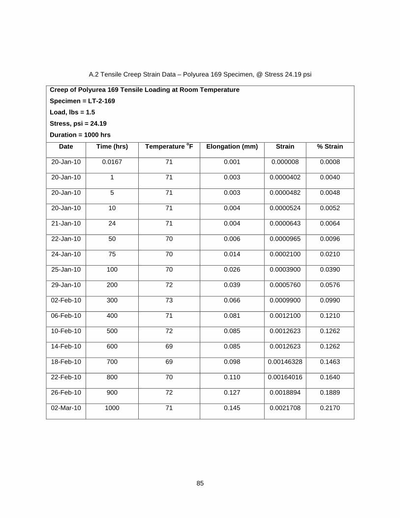
85
A.2 Tensile Creep Strain Data – Polyurea 169 Specimen, @ Stress 24.19 psi
Creep of Polyurea 169 Tensile Loading at Room Tempe rature
Specimen = LT-2-169
Load, lbs = 1.5
Stress, psi = 24.19
Duration = 1000 hrs
Date Time (hrs) Temperature oF Elongation (mm) Strain % Strain
20-Jan-10 0.0167 71 0.001 0.000008 0.0008
20-Jan-10 1 71 0.003 0.0000402 0.0040
20-Jan-10 5 71 0.003 0.0000482 0.0048
20-Jan-10 10 71 0.004 0.0000524 0.0052
21-Jan-10 24 71 0.004 0.0000643 0.0064
22-Jan-10 50 70 0.006 0.0000965 0.0096
24-Jan-10 75 70 0.014 0.0002100 0.0210
25-Jan-10 100 70 0.026 0.0003900 0.0390
29-Jan-10 200 72 0.039 0.0005760 0.0576
02-Feb-10 300 73 0.066 0.0009900 0.0990
06-Feb-10 400 71 0.081 0.0012100 0.1210
10-Feb-10 500 72 0.085 0.0012623 0.1262
14-Feb-10 600 69 0.085 0.0012623 0.1262
18-Feb-10 700 69 0.098 0.00146328 0.1463
22-Feb-10 800 70 0.110 0.00164016 0.1640
26-Feb-10 900 72 0.127 0.0018894 0.1889
02-Mar-10 1000 71 0.145 0.0021708 0.2170

86
A.3 Tensile Creep Strain Data – Polyurea 169 Specimen, @ Stress 28.22 psi
Creep of Polyurea 169 Tensile Loading at Room Tempe rature
Specimen = LT-3-169
Load, lbs = 1.75
Stress, psi = 28.22
Duration = 1000 hrs
Date Time (hrs) Temperature oF Elongation (mm) Strain % Strain
20-Jan-10 0.0167 71 0.005 0.000076 0.0076
20-Jan-10 1 71 0.007 0.000109 0.0109
20-Jan-10 5 71 0.009 0.000129 0.0129
20-Jan-10 10 71 0.009 0.000134 0.0134
21-Jan-10 24 71 0.009 0.000136 0.0136
22-Jan-10 50 70 0.010 0.000150 0.0150
24-Jan-10 75 70 0.010 0.000155 0.0155
25-Jan-10 100 70 0.011 0.000161 0.0161
29-Jan-10 200 72 0.034 0.000503 0.0503
02-Feb-10 300 73 0.043 0.000639 0.0639
06-Feb-10 400 71 0.068 0.001013 0.1013
10-Feb-10 500 72 0.084 0.001258 0.1258
14-Feb-10 600 69 0.099 0.001479 0.1479
18-Feb-10 700 69 0.101 0.001503 0.1503
22-Feb-10 800 70 0.106 0.001588 0.1588
26-Feb-10 900 72 0.112 0.001668 0.1668
02-Mar-10 1000 71 0.116 0.001737 0.1737

87
A.4 Tensile Creep Strain Data – Polyurea 169HB Specimen, @ Stress 32.25 psi
Creep of Polyurea 169HB Tensile Loading at Room Temperature
Specimen = LT-4-169HB
Load, lbs = 2
Stress, psi = 32.25
Duration = 1000 hrs
Date Time (hrs) Temperature oF Elongation (mm) Strain % Strain
20-Jan-10 0.0167 71 0.001 0.000012 0.0012
20-Jan-10 1 71 0.017 0.000249 0.0249
20-Jan-10 5 71 0.018 0.000261 0.0261
20-Jan-10 10 71 0.018 0.000265 0.0265
21-Jan-10 24 71 0.018 0.000274 0.0273
22-Jan-10 50 70 0.019 0.000285 0.0285
24-Jan-10 75 70 0.021 0.000310 0.0309
25-Jan-10 100 70 0.025 0.000370 0.0369
29-Jan-10 200 72 0.034 0.000515 0.0514
02-Feb-10 300 73 0.040 0.000591 0.0590
06-Feb-10 400 71 0.058 0.000872 0.0872
10-Feb-10 500 72 0.063 0.000945 0.0944
14-Feb-10 600 69 0.082 0.001218 0.1218
18-Feb-10 700 69 0.086 0.001278 0.1278
22-Feb-10 800 70 0.089 0.001331 0.1330
26-Feb-10 900 72 0.090 0.001351 0.1350
02-Mar-10 1000 71 0.092 0.001375 0.1374

88
A.5 Tensile Creep Strain Data – Polyurea 169HB Specimen, @ Stress 48.38 psi
Creep of Polyurea 169HB Tensile Loading at Room Temperature
Specimen = LT-5-169HB
Load, lbs = 3.0
Stress, psi = 48.38
Duration = 1000 hrs
Date Time (hrs) Temperature oF Elongation (mm) Strain % Strain
22-Jan-10 0.0167 70 0.012 0.000181 0.0181
22-Jan-10 1 70 0.040 0.000591 0.0591
22-Jan-10 5 70 0.044 0.000663 0.0663
22-Jan-10 10 70 0.046 0.000686 0.0686
23-Jan-10 24 73 0.050 0.000740 0.0740
24-Jan-10 50 71 0.054 0.000804 0.0804
27-Jan-10 75 72 0.060 0.000898 0.0898
28-Jan-10 100 69 0.076 0.001134 0.1134
01-Feb-10 200 69 0.085 0.001270 0.1270
05-Feb-10 300 70 0.088 0.001319 0.1319
09-Feb-10 400 72 0.088 0.001319 0.1319
13-Feb-10 500 71 0.096 0.001431 0.1431
17-Feb-10 600 70 0.110 0.001636 0.1636
21-Feb-10 700 70 0.113 0.001684 0.1684
25-Feb-10 800 70 0.117 0.001749 0.1749
01-Mar-10 900 72 0.119 0.001769 0.1769
05-Mar-10 1000 73 0.123 0.001837 0.1837
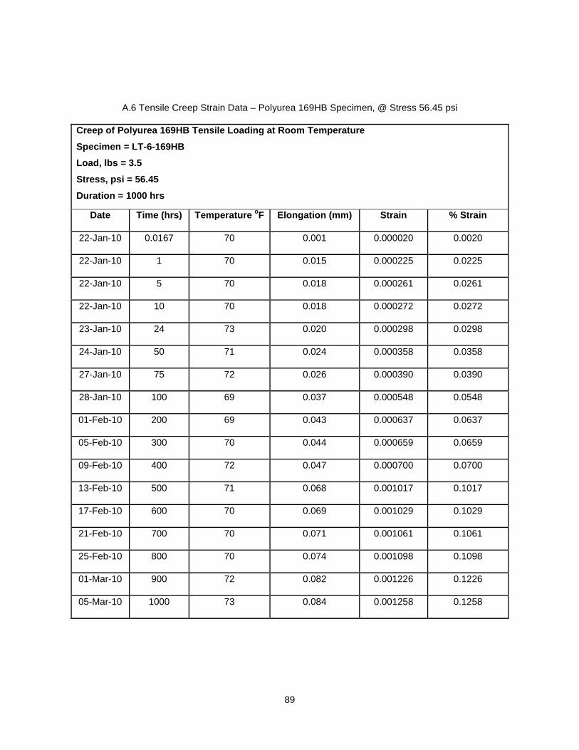
89
A.6 Tensile Creep Strain Data – Polyurea 169HB Specimen, @ Stress 56.45 psi
Creep of Polyurea 169HB Tensile Loading at Room Tem perature
Specimen = LT-6-169HB
Load, lbs = 3.5
Stress, psi = 56.45
Duration = 1000 hrs
Date Time (hrs) Temperature oF Elongation (mm) Strain % Strain
22-Jan-10 0.0167 70 0.001 0.000020 0.0020
22-Jan-10 1 70 0.015 0.000225 0.0225
22-Jan-10 5 70 0.018 0.000261 0.0261
22-Jan-10 10 70 0.018 0.000272 0.0272
23-Jan-10 24 73 0.020 0.000298 0.0298
24-Jan-10 50 71 0.024 0.000358 0.0358
27-Jan-10 75 72 0.026 0.000390 0.0390
28-Jan-10 100 69 0.037 0.000548 0.0548
01-Feb-10 200 69 0.043 0.000637 0.0637
05-Feb-10 300 70 0.044 0.000659 0.0659
09-Feb-10 400 72 0.047 0.000700 0.0700
13-Feb-10 500 71 0.068 0.001017 0.1017
17-Feb-10 600 70 0.069 0.001029 0.1029
21-Feb-10 700 70 0.071 0.001061 0.1061
25-Feb-10 800 70 0.074 0.001098 0.1098
01-Mar-10 900 72 0.082 0.001226 0.1226
05-Mar-10 1000 73 0.084 0.001258 0.1258
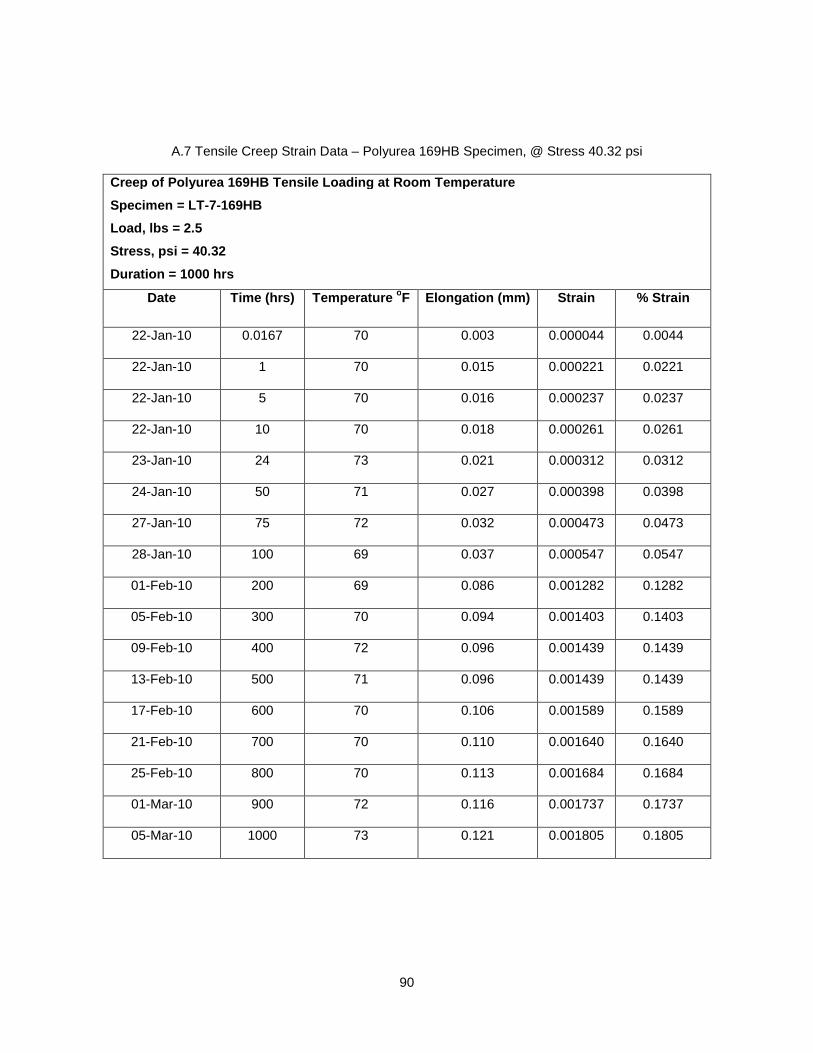
90
A.7 Tensile Creep Strain Data – Polyurea 169HB Specimen, @ Stress 40.32 psi
Creep of Poly urea 169HB Tensile Loading at Room Temperature
Specimen = LT-7-169HB
Load, lbs = 2.5
Stress, psi = 40.32
Duration = 1000 hrs
Date Time (hrs) Temperature oF Elongation (mm) Strain % Strain
22-Jan-10 0.0167 70 0.003 0.000044 0.0044
22-Jan-10 1 70 0.015 0.000221 0.0221
22-Jan-10 5 70 0.016 0.000237 0.0237
22-Jan-10 10 70 0.018 0.000261 0.0261
23-Jan-10 24 73 0.021 0.000312 0.0312
24-Jan-10 50 71 0.027 0.000398 0.0398
27-Jan-10 75 72 0.032 0.000473 0.0473
28-Jan-10 100 69 0.037 0.000547 0.0547
01-Feb-10 200 69 0.086 0.001282 0.1282
05-Feb-10 300 70 0.094 0.001403 0.1403
09-Feb-10 400 72 0.096 0.001439 0.1439
13-Feb-10 500 71 0.096 0.001439 0.1439
17-Feb-10 600 70 0.106 0.001589 0.1589
21-Feb-10 700 70 0.110 0.001640 0.1640
25-Feb-10 800 70 0.113 0.001684 0.1684
01-Mar-10 900 72 0.116 0.001737 0.1737
05-Mar-10 1000 73 0.121 0.001805 0.1805
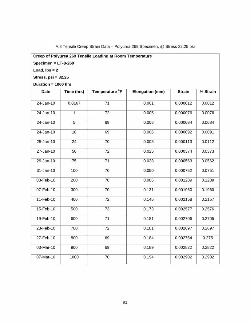
91
A.8 Tensile Creep Strain Data – Polyurea 269 Specimen, @ Stress 32.25 psi
Creep of Polyurea 269 Tensile Loading at Room Temperature
Specimen = LT-8-269
Load, lbs = 2
Stress, psi = 32.25
Duration = 1000 hrs
Date Time (hrs) Temperature oF Elongation (mm) Strain % Strain
24-Jan-10 0.0167 71 0.001 0.000012 0.0012
24-Jan-10 1 72 0.005 0.000076 0.0076
24-Jan-10 5 69 0.006 0.000084 0.0084
24-Jan-10 10 69 0.006 0.000092 0.0091
25-Jan-10 24 70 0.008 0.000113 0.0112
27-Jan-10 50 72 0.025 0.000374 0.0373
29-Jan-10 75 71 0.038 0.000563 0.0562
31-Jan-10 100 70 0.050 0.000752 0.0751
03-Feb-10 200 70 0.086 0.001289 0.1289
07-Feb-10 300 70 0.131 0.001960 0.1960
11-Feb-10 400 72 0.145 0.002158 0.2157
15-Feb-10 500 73 0.173 0.002577 0.2576
19-Feb-10 600 71 0.181 0.002706 0.2705
23-Feb-10 700 72 0.181 0.002697 0.2697
27-Feb-10 800 69 0.184 0.002754 0.275
03-Mar-10 900 69 0.189 0.002822 0.2822
07-Mar-10 1000 70 0.194 0.002902 0.2902

92
A.9 Tensile Creep Strain Data – Polyurea 269 Specimen, @ Stress 32.25 psi
Creep of Polyurea 269 Tensile Loading at Room Tempe rature
Specimen = LT-9-269
Load, lbs = 2
Stress, psi = 32.25
Duration = 1000 hrs
Date Time (hrs) Temperature oF Elongation (mm) Strain % Strain
24-Jan-10 0.0167 71 0.005 0.000080 0.0080
24-Jan-10 1 71 0.007 0.000105 0.0105
24-Jan-10 5 71 0.011 0.000157 0.0157
24-Jan-10 10 71 0.012 0.000176 0.0176
25-Jan-10 24 70 0.015 0.000225 0.0225
27-Jan-10 50 72 0.027 0.000402 0.0402
29-Jan-10 75 71 0.042 0.000621 0.0621
31-Jan-10 100 70 0.046 0.000694 0.0694
03-Feb-10 200 70 0.108 0.001608 0.1608
07-Feb-10 300 70 0.111 0.001664 0.1664
11-Feb-10 400 72 0.130 0.001938 0.1938
15-Feb-10 500 73 0.151 0.002251 0.2251
19-Feb-10 600 71 0.159 0.002368 0.2368
23-Feb-10 700 72 0.167 0.002488 0.2488
27-Feb-10 800 69 0.177 0.002645 0.2645
03-Mar-10 900 69 0.188 0.002810 0.2810
07-Mar-10 1000 70 0.197 0.002947 0.2947
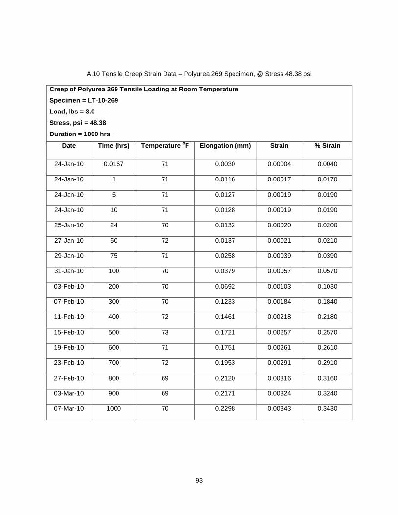
93
A.10 Tensile Creep Strain Data – Polyurea 269 Specimen, @ Stress 48.38 psi
Creep of Polyurea 269 Tensile Loading at Room Tempe rature
Specimen = LT-10-269
Load, lbs = 3.0
Stress, psi = 48.38
Duration = 1000 hrs
Date Time (hrs) Temperature oF Elongation (mm) Strain % Strain
24-Jan-10 0.0167 71 0.0030 0.00004 0.0040
24-Jan-10 1 71 0.0116 0.00017 0.0170
24-Jan-10 5 71 0.0127 0.00019 0.0190
24-Jan-10 10 71 0.0128 0.00019 0.0190
25-Jan-10 24 70 0.0132 0.00020 0.0200
27-Jan-10 50 72 0.0137 0.00021 0.0210
29-Jan-10 75 71 0.0258 0.00039 0.0390
31-Jan-10 100 70 0.0379 0.00057 0.0570
03-Feb-10 200 70 0.0692 0.00103 0.1030
07-Feb-10 300 70 0.1233 0.00184 0.1840
11-Feb-10 400 72 0.1461 0.00218 0.2180
15-Feb-10 500 73 0.1721 0.00257 0.2570
19-Feb-10 600 71 0.1751 0.00261 0.2610
23-Feb-10 700 72 0.1953 0.00291 0.2910
27-Feb-10 800 69 0.2120 0.00316 0.3160
03-Mar-10 900 69 0.2171 0.00324 0.3240
07-Mar-10 1000 70 0.2298 0.00343 0.3430
94
APPENDIX B
TENSILE CREEP STRAIN GRAPHS

95
B.1 Tensile Creep Strain Graph – Polyurea169 Specimen, @ Stress 24.19 psi
Figure B.1 – Strain (%) vs. Time (hours) for Polyur ea 169
B.2 Tensile Creep Strain Graph – Polyurea 169 Specimen, @ Stress 24.19 psi
Figure B.2 – Strain (%) vs. Time (hours) for Polyur ea 169
0.0000
0.0600
0.1200
0.1800
0 200 400 600 800 1000
Str
ain
, %
Time, hrs
0
0.06
0.12
0.18
0.24
0 200 400 600 800 1000
Str
ain
, %
Time , hrs

96
B.3 Tensile Creep Strain Graph – Polyurea 169 Specimen, @ Stress 28.22 psi
Figure B.3 – Strain (%) vs. Time (hours) for Polyur ea 169
B.4 Tensile Creep Strain Graph – Polyurea 169HB Specimen, @ Stress 32.25 psi
Figure B.4 – Strain (%) vs. Time (hours) for Polyur ea 169HB
0
0.06
0.12
0.18
0 200 400 600 800 1000
Str
ian
, %
Time, hrs
0
0.06
0.12
0.18
0 200 400 600 800 1000
Str
ain
, %
Time, hrs
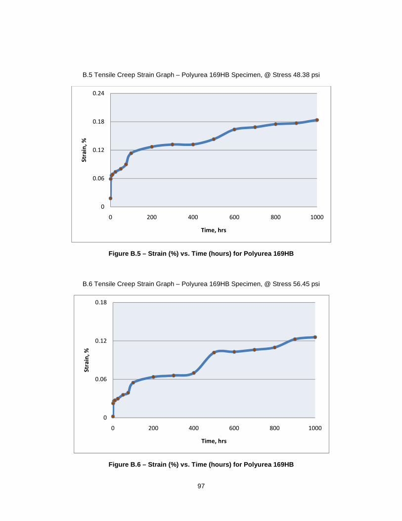
97
B.5 Tensile Creep Strain Graph – Polyurea 169HB Specimen, @ Stress 48.38 psi
Figure B.5 – Strain (%) vs. Time (hours) for Polyur ea 169HB
B.6 Tensile Creep Strain Graph – Polyurea 169HB Specimen, @ Stress 56.45 psi
Figure B.6 – Strain (%) vs. Time (hours) for Polyur ea 169HB
0
0.06
0.12
0.18
0.24
0 200 400 600 800 1000
Str
ain
, %
Time, hrs
0
0.06
0.12
0.18
0 200 400 600 800 1000
Str
ain
, %
Time, hrs
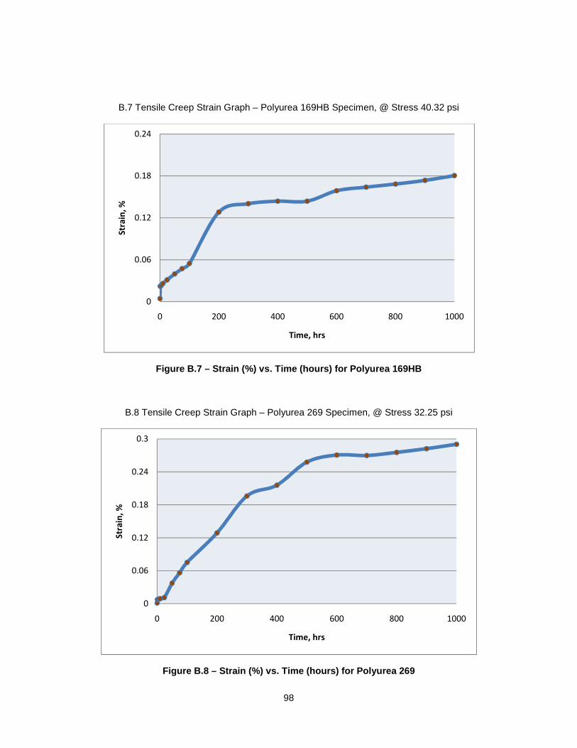
98
B.7 Tensile Creep Strain Graph – Polyurea 169HB Specimen, @ Stress 40.32 psi
Figure B.7 – Strain (%) vs. Time (hours) for Polyur ea 169HB
B.8 Tensile Creep Strain Graph – Polyurea 269 Specimen, @ Stress 32.25 psi
Figure B.8 – Strain (%) vs. Time (hours) for Polyur ea 269
0
0.06
0.12
0.18
0.24
0 200 400 600 800 1000
Str
ain
, %
Time, hrs
0
0.06
0.12
0.18
0.24
0.3
0 200 400 600 800 1000
Str
ain
, %
Time, hrs

99
B.9 Tensile Creep Strain Graph – Polyurea 269 Specimen, @ Stress 32.25 psi
Figure B.9 – Strain (%) vs. Time (hours) for Polyur ea 269
B.10 Tensile Creep Strain Graph – Polyurea 269 Specimen, @ Stress 48.38 psi
Figure B.10 – Strain (%) vs. Time (hours) for Polyu rea 269
0
0.06
0.12
0.18
0.24
0.3
0 200 400 600 800 1000
Str
ain
, %
Time, hrs
0.00
0.06
0.12
0.18
0.24
0.30
0.36
0 200 400 600 800 1000
Str
ian
, %
Time, hrs
100
APPENDIX C
TENSILE CREEP MODULUS GRAPHS
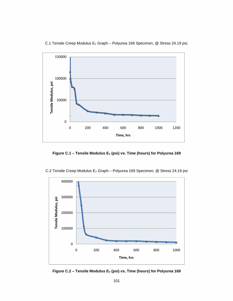
101
C.1 Tensile Creep Modulus ET Graph – Polyurea 169 Specimen, @ Stress 24.19 psi.
Figure C.1 – Tensile Modulus E T (psi) vs. Time (hours) for Polyurea 169
C.2 Tensile Creep Modulus ET Graph – Polyurea 169 Specimen, @ Stress 24.19 psi
Figure C.2 – Tensile Modulus E T (psi) vs. Time (hours) for Polyurea 169
0
100000
200000
300000
400000
0 200 400 600 800 1000
Te
nsi
le M
od
ulu
s, p
si
Time, hrs
0
50000
100000
150000
0 200 400 600 800 1000 1200
Te
nsi
le M
od
ulu
s, p
si
Time, hrs

102
C.3 Tensile Creep Modulus ET Graph – Polyurea 169 Specimen, @ Stress 28.22 psi
Figure C.3 – Tensile Modulus E T (psi) vs. Time (hours) for Polyurea 169
C.4 Tensile Creep Modulus ET Graph – Polyurea 169HB Specimen, @ Stress 32.25 psi
Figure C.4 – Tensile Modulus E T (psi) vs. Time (hours) for Polyurea 169HB
0
100000
200000
300000
0 200 400 600 800 1000
Te
nsi
le M
od
ulu
s, p
si
Time, hrs
0
100000
200000
300000
0 200 400 600 800 1000
Te
nsi
le M
od
ulu
s, p
si
Time, hrs
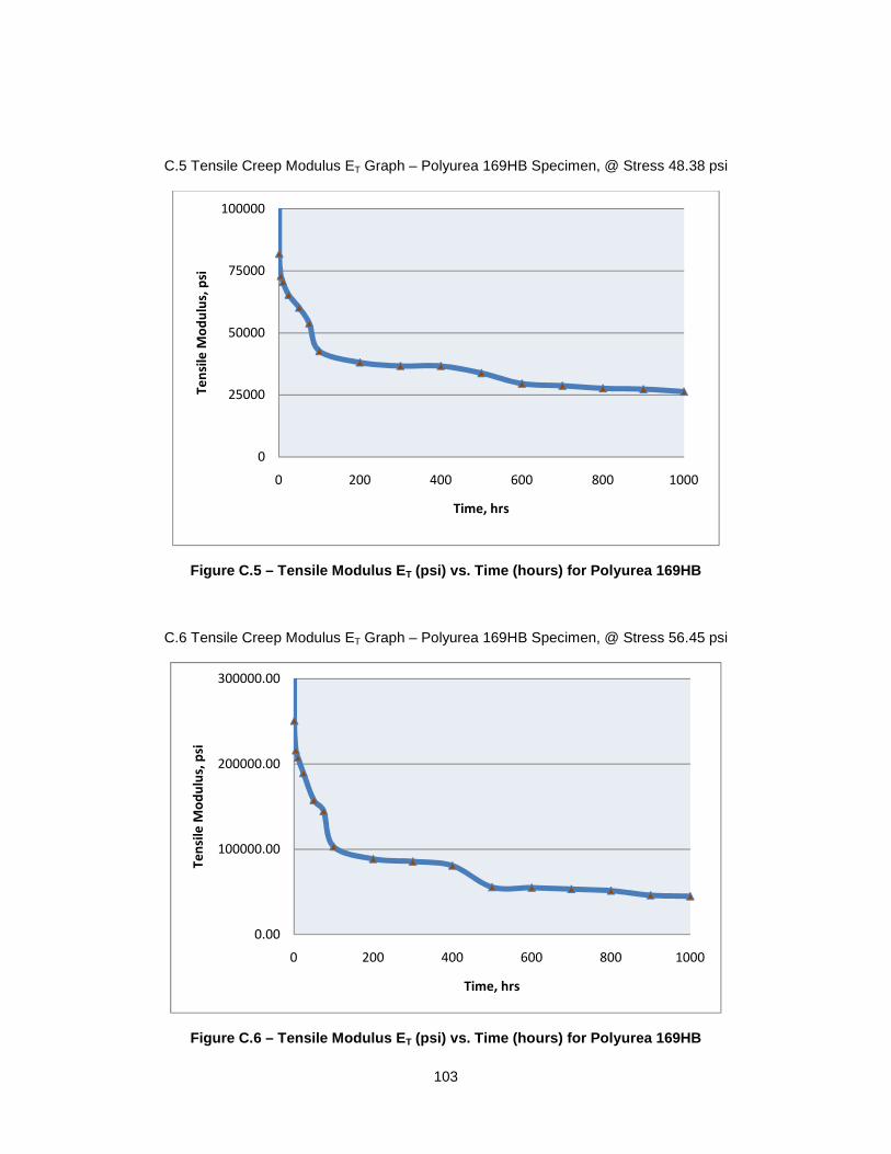
103
C.5 Tensile Creep Modulus ET Graph – Polyurea 169HB Specimen, @ Stress 48.38 psi
Figure C.5 – Tensile Modulus E T (psi) vs. Time (hours) for Polyurea 169HB
C.6 Tensile Creep Modulus ET Graph – Polyurea 169HB Specimen, @ Stress 56.45 psi
Figure C.6 – Tensile Modulus E T (psi) vs. Time (hours) for Polyurea 169HB
0
25000
50000
75000
100000
0 200 400 600 800 1000
Te
nsi
le M
od
ulu
s, p
si
Time, hrs
0.00
100000.00
200000.00
300000.00
0 200 400 600 800 1000
Te
nsi
le M
od
ulu
s, p
si
Time, hrs

104
C.7 Tensile Creep Modulus ET Graph – Polyurea 169HB Specimen, @ Stress 40.32 psi
Figure C.7 – Tensile Modulus E T (psi) vs. Time (hours) for Polyurea 169HB
C.8 Tensile Creep Modulus ET Graph – Polyurea 269 Specimen, @ Stress 32.25 psi
Figure C.8 – Tensile Modulus E T (psi) vs. Time (hours) for Polyurea 269
0
100000
200000
300000
0 200 400 600 800 1000
Te
nsi
le M
od
ulu
s, p
si
Time, hrs
0
100000
200000
300000
400000
0 200 400 600 800 1000
Te
nsi
le M
od
ulu
s, p
si
Time, hrs

105
C.9 Tensile Creep Modulus ET Graph – Polyurea 269 Specimen, @ Stress 32.25 psi
Figure C.9 – Tensile Modulus E T (psi) vs. Time (hours) for Polyurea 269
C.10 Tensile Creep Modulus ET Graph – Polyurea 269 Specimen, @ Stress 48.38 psi
Figure C.10 – Tensile Modulus E T (psi) vs. Time (hours) for Polyurea 269
0
50000
100000
150000
200000
250000
0 200 400 600 800 1000
Te
nsi
le M
od
ulu
s, p
si
Time, hrs
0.00
100000.00
200000.00
300000.00
0 200 400 600 800 1000
Te
nsi
le M
od
ulu
s, p
si
Time, hrs
106
APPENDIX D
FLEXURAL CREEP STRAIN DATA
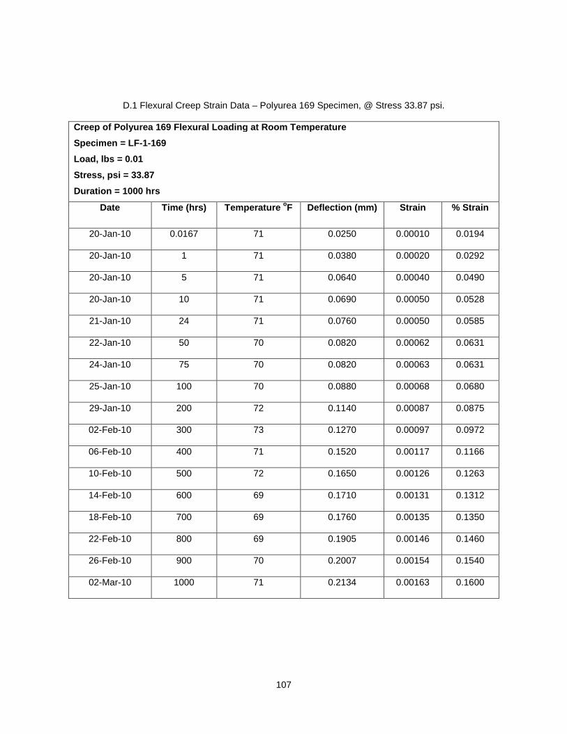
107
D.1 Flexural Creep Strain Data – Polyurea 169 Specimen, @ Stress 33.87 psi.
Creep of Polyurea 169 Flexural Loading at Room Temp erature
Specimen = LF-1-169
Load, lbs = 0.01
Stress, psi = 33.87
Duration = 1000 hrs
Date Time (hrs) Temperature oF Deflection (mm) Strain % Strain
20-Jan-10 0.0167 71 0.0250 0.00010 0.0194
20-Jan-10 1 71 0.0380 0.00020 0.0292
20-Jan-10 5 71 0.0640 0.00040 0.0490
20-Jan-10 10 71 0.0690 0.00050 0.0528
21-Jan-10 24 71 0.0760 0.00050 0.0585
22-Jan-10 50 70 0.0820 0.00062 0.0631
24-Jan-10 75 70 0.0820 0.00063 0.0631
25-Jan-10 100 70 0.0880 0.00068 0.0680
29-Jan-10 200 72 0.1140 0.00087 0.0875
02-Feb-10 300 73 0.1270 0.00097 0.0972
06-Feb-10 400 71 0.1520 0.00117 0.1166
10-Feb-10 500 72 0.1650 0.00126 0.1263
14-Feb-10 600 69 0.1710 0.00131 0.1312
18-Feb-10 700 69 0.1760 0.00135 0.1350
22-Feb-10 800 69 0.1905 0.00146 0.1460
26-Feb-10 900 70 0.2007 0.00154 0.1540
02-Mar-10 1000 71 0.2134 0.00163 0.1600

108
D.2 Flexural Creep Strain Data – Polyurea 169 Specimen, @ Stress 27.09 psi.
Creep of Polyurea 169 Flexural Loading at Room Temp erature
Specimen = LF-2-169
Load, lbs = 0.08
Stress, psi = 27.097
Duration = 1000 hrs
Date Time (hrs) Temperature oF Deflection (mm) Strain % Strain
20-Jan-10 0.0167 71 0.0200 0.00010 0.0153
20-Jan-10 1 71 0.0400 0.00030 0.0306
20-Jan-10 5 71 0.0500 0.00030 0.0383
20-Jan-10 10 71 0.0550 0.00040 0.0421
21-Jan-10 24 71 0.0650 0.00050 0.0497
22-Jan-10 50 70 0.0850 0.00060 0.0651
24-Jan-10 75 70 0.0900 0.00060 0.0689
25-Jan-10 100 70 0.0950 0.00070 0.0727
29-Jan-10 200 72 0.1100 0.00080 0.0842
02-Feb-10 300 73 0.1450 0.00110 0.1110
06-Feb-10 400 71 0.1735 0.00133 0.1330
10-Feb-10 500 72 0.1775 0.00136 0.1360
14-Feb-10 600 69 0.1800 0.00138 0.1378
18-Feb-10 700 69 0.1835 0.00140 0.1404
22-Feb-10 800 69 0.1895 0.00145 0.1450
26-Feb-10 900 70 0.1930 0.00148 0.1477
02-Mar-10 1000 71 0.1945 0.00149 0.1488

109
D.3 Flexural Creep Strain Data – Polyurea 169 Specimen, @ Stress 40.64 psi.
Creep of P olyurea 169 Flexural Loading at Room Temperature
Specimen = LF-3-169
Load, lbs = 0.12
Stress, psi = 40.64
Duration = 1000 hrs
Date Time (hrs) Temperature oF Deflection (mm) Strain % Strain
22-Jan-10 0.0167 71 0.030 0.00020 0.023
22-Jan-10 1 71 0.045 0.00030 0.034
22-Jan-10 5 71 0.055 0.00040 0.042
22-Jan-10 10 71 0.060 0.00040 0.046
23-Jan-10 24 71 0.070 0.00050 0.054
24-Jan-10 50 70 0.100 0.00070 0.077
27-Jan-10 75 70 0.105 0.00080 0.080
28-Jan-10 100 70 0.115 0.00080 0.088
01-Feb-10 200 72 0.130 0.00090 0.100
05-Feb-10 300 73 0.190 0.00140 0.145
09-Feb-10 400 71 0.230 0.00176 0.176
13-Feb-10 500 72 0.230 0.00176 0.176
17-Feb-10 600 69 0.240 0.00184 0.184
21-Feb-10 700 69 0.245 0.00188 0.188
25-Feb-10 800 69 0.248 0.00189 0.189
01-Mar-10 900 71 0.250 0.00191 0.191
05-Mar-10 1000 70 0.253 0.00193 0.193
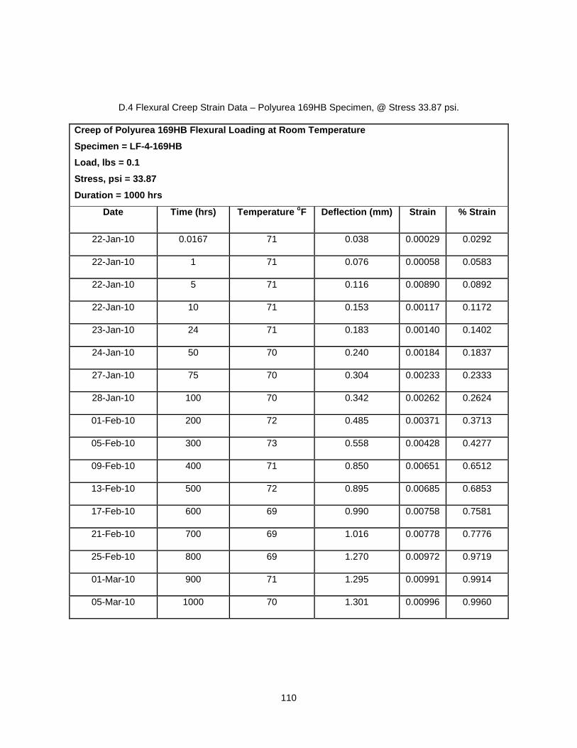
110
D.4 Flexural Creep Strain Data – Polyurea 169HB Specimen, @ Stress 33.87 psi.
Creep of Polyurea 169HB Flexural Loading at Room Te mperature
Specimen = LF-4-169HB
Load, lbs = 0.1
Stress, psi = 33.87
Duration = 1000 hrs
Date Time (hrs) Temperature oF Deflection (mm) Strain % Strain
22-Jan-10 0.0167 71 0.038 0.00029 0.0292
22-Jan-10 1 71 0.076 0.00058 0.0583
22-Jan-10 5 71 0.116 0.00890 0.0892
22-Jan-10 10 71 0.153 0.00117 0.1172
23-Jan-10 24 71 0.183 0.00140 0.1402
24-Jan-10 50 70 0.240 0.00184 0.1837
27-Jan-10 75 70 0.304 0.00233 0.2333
28-Jan-10 100 70 0.342 0.00262 0.2624
01-Feb-10 200 72 0.485 0.00371 0.3713
05-Feb-10 300 73 0.558 0.00428 0.4277
09-Feb-10 400 71 0.850 0.00651 0.6512
13-Feb-10 500 72 0.895 0.00685 0.6853
17-Feb-10 600 69 0.990 0.00758 0.7581
21-Feb-10 700 69 1.016 0.00778 0.7776
25-Feb-10 800 69 1.270 0.00972 0.9719
01-Mar-10 900 71 1.295 0.00991 0.9914
05-Mar-10 1000 70 1.301 0.00996 0.9960
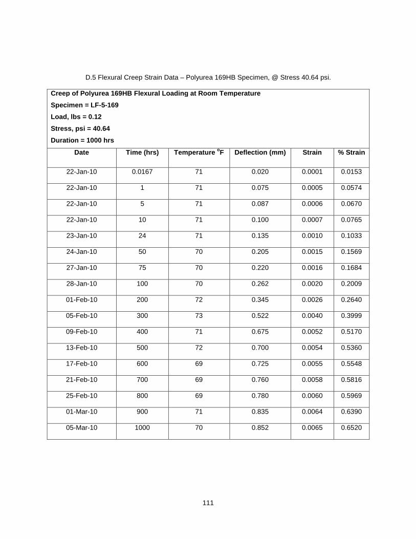
111
D.5 Flexural Creep Strain Data – Polyurea 169HB Specimen, @ Stress 40.64 psi.
Creep of Polyurea 169HB Flexural Loading at Room Te mperature
Specimen = LF-5-169
Load, lbs = 0.12
Stress, psi = 40.64
Duration = 1000 hrs
Date Time (hrs) Temperature oF Deflection (mm) Strain % Strain
22-Jan-10 0.0167 71 0.020 0.0001 0.0153
22-Jan-10 1 71 0.075 0.0005 0.0574
22-Jan-10 5 71 0.087 0.0006 0.0670
22-Jan-10 10 71 0.100 0.0007 0.0765
23-Jan-10 24 71 0.135 0.0010 0.1033
24-Jan-10 50 70 0.205 0.0015 0.1569
27-Jan-10 75 70 0.220 0.0016 0.1684
28-Jan-10 100 70 0.262 0.0020 0.2009
01-Feb-10 200 72 0.345 0.0026 0.2640
05-Feb-10 300 73 0.522 0.0040 0.3999
09-Feb-10 400 71 0.675 0.0052 0.5170
13-Feb-10 500 72 0.700 0.0054 0.5360
17-Feb-10 600 69 0.725 0.0055 0.5548
21-Feb-10 700 69 0.760 0.0058 0.5816
25-Feb-10 800 69 0.780 0.0060 0.5969
01-Mar-10 900 71 0.835 0.0064 0.6390
05-Mar-10 1000 70 0.852 0.0065 0.6520
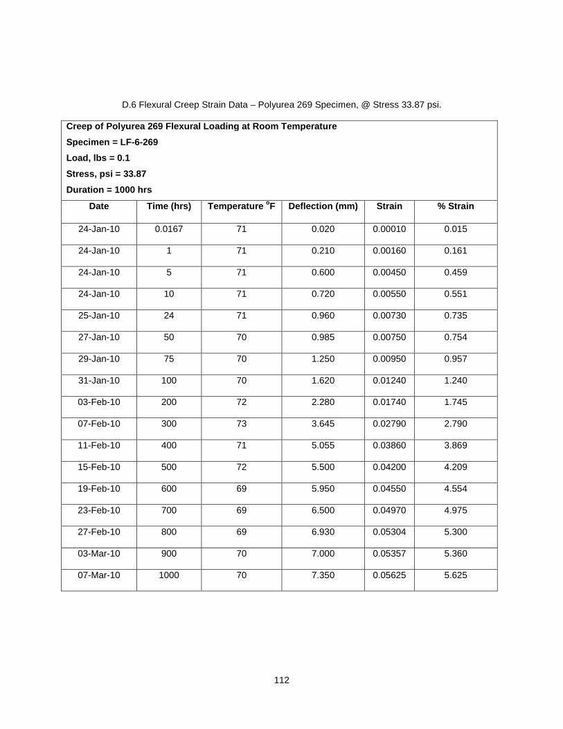
112
D.6 Flexural Creep Strain Data – Polyurea 269 Specimen, @ Stress 33.87 psi. Creep of Polyurea 269 Flexural Loading at Room Temperature
Specimen = LF-6-269
Load, lbs = 0.1
Stress, psi = 33.87
Duration = 1000 hrs
Date Time (hrs) Temperature oF Deflection (mm) Strain % Strain
24-Jan-10 0.0167 71 0.020 0.00010 0.015
24-Jan-10 1 71 0.210 0.00160 0.161
24-Jan-10 5 71 0.600 0.00450 0.459
24-Jan-10 10 71 0.720 0.00550 0.551
25-Jan-10 24 71 0.960 0.00730 0.735
27-Jan-10 50 70 0.985 0.00750 0.754
29-Jan-10 75 70 1.250 0.00950 0.957
31-Jan-10 100 70 1.620 0.01240 1.240
03-Feb-10 200 72 2.280 0.01740 1.745
07-Feb-10 300 73 3.645 0.02790 2.790
11-Feb-10 400 71 5.055 0.03860 3.869
15-Feb-10 500 72 5.500 0.04200 4.209
19-Feb-10 600 69 5.950 0.04550 4.554
23-Feb-10 700 69 6.500 0.04970 4.975
27-Feb-10 800 69 6.930 0.05304 5.300
03-Mar-10 900 70 7.000 0.05357 5.360
07-Mar-10 1000 70 7.350 0.05625 5.625
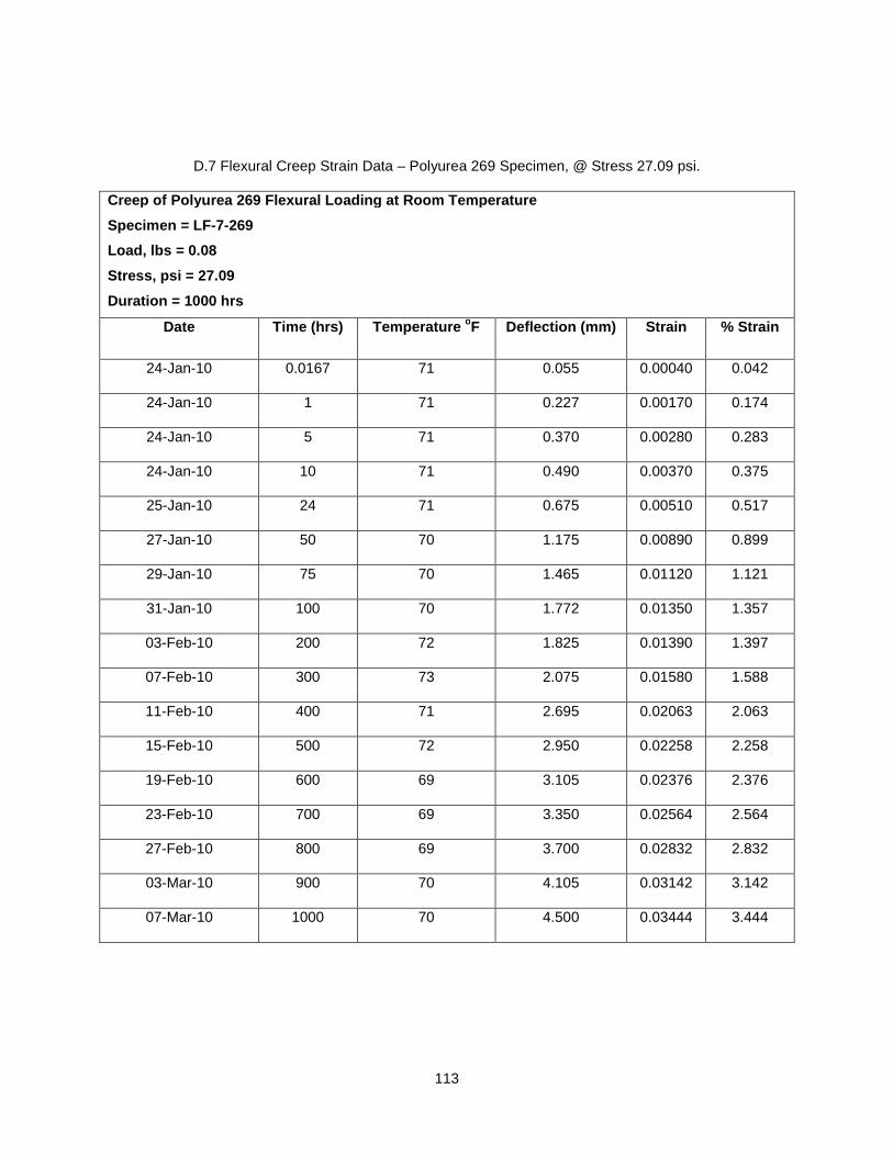
113
D.7 Flexural Creep Strain Data – Polyurea 269 Specimen, @ Stress 27.09 psi.
Creep of Polyurea 269 Flexural Loading at Room Temp erature
Specimen = LF-7-269
Load, lbs = 0.08
Stress, psi = 27.09
Duration = 1000 hrs
Date Time (hrs) Temperature oF Deflection (mm) Strain % Strain
24-Jan-10 0.0167 71 0.055 0.00040 0.042
24-Jan-10 1 71 0.227 0.00170 0.174
24-Jan-10 5 71 0.370 0.00280 0.283
24-Jan-10 10 71 0.490 0.00370 0.375
25-Jan-10 24 71 0.675 0.00510 0.517
27-Jan-10 50 70 1.175 0.00890 0.899
29-Jan-10 75 70 1.465 0.01120 1.121
31-Jan-10 100 70 1.772 0.01350 1.357
03-Feb-10 200 72 1.825 0.01390 1.397
07-Feb-10 300 73 2.075 0.01580 1.588
11-Feb-10 400 71 2.695 0.02063 2.063
15-Feb-10 500 72 2.950 0.02258 2.258
19-Feb-10 600 69 3.105 0.02376 2.376
23-Feb-10 700 69 3.350 0.02564 2.564
27-Feb-10 800 69 3.700 0.02832 2.832
03-Mar-10 900 70 4.105 0.03142 3.142
07-Mar-10 1000 70 4.500 0.03444 3.444

114
D.8 Flexural Creep Strain Data – Polyurea 269 Specimen, @ Stress 20.32 psi.
Creep of Polyurea 269 Flexural Loading at Room Temperature
Specimen = LF-8-269
Load, lbs = 0.06
Stress, psi = 20.32
Duration = 1000 hrs
Date Time (hrs) Temperature oF Deflection (mm) Strain % Strain
24-Jan-10 0.0167 71 0.055 0.00042 0.042
24-Jan-10 1 71 0.150 0.00115 0.115
24-Jan-10 5 71 0.235 0.00180 0.180
24-Jan-10 10 71 0.290 0.00222 0.222
25-Jan-10 24 71 0.420 0.00321 0.321
27-Jan-10 50 70 0.705 0.00540 0.540
29-Jan-10 75 70 0.900 0.00689 0.689
31-Jan-10 100 70 1.070 0.00819 0.819
03-Feb-10 200 72 1.740 0.01332 1.332
07-Feb-10 300 73 2.420 0.01852 1.852
11-Feb-10 400 71 3.450 0.02640 2.640
15-Feb-10 500 72 3.770 0.02885 2.890
19-Feb-10 600 69 3.990 0.03054 3.050
23-Feb-10 700 69 4.290 0.03283 3.280
27-Feb-10 800 69 4.480 0.03429 3.430
03-Mar-10 900 70 4.850 0.03712 3.710
07-Mar-10 1000 70 5.200 0.03980 3.980

115
APPENDIX E
FLEXURAL CREEP STRAIN GRAPH

116
E.1 Flexural Creep Strain Data – Polyurea 169 Specimen, @ Stress 33.87 psi
Figure E.1 – Strain (%) vs. Time (hours) for Polyur ea 169
E.2 Flexural Creep Strain Data – Polyurea 169 Specimen, @ Stress 27.09 psi
Figure E.2 – Strain (%) vs. Time (hours) for Polyur ea 169
0
0.06
0.12
0.18
0 200 400 600 800 1000
Str
ain
, %
Time, hrs
0
0.06
0.12
0.18
0 200 400 600 800 1000
Str
ain
, %
Time, hrs
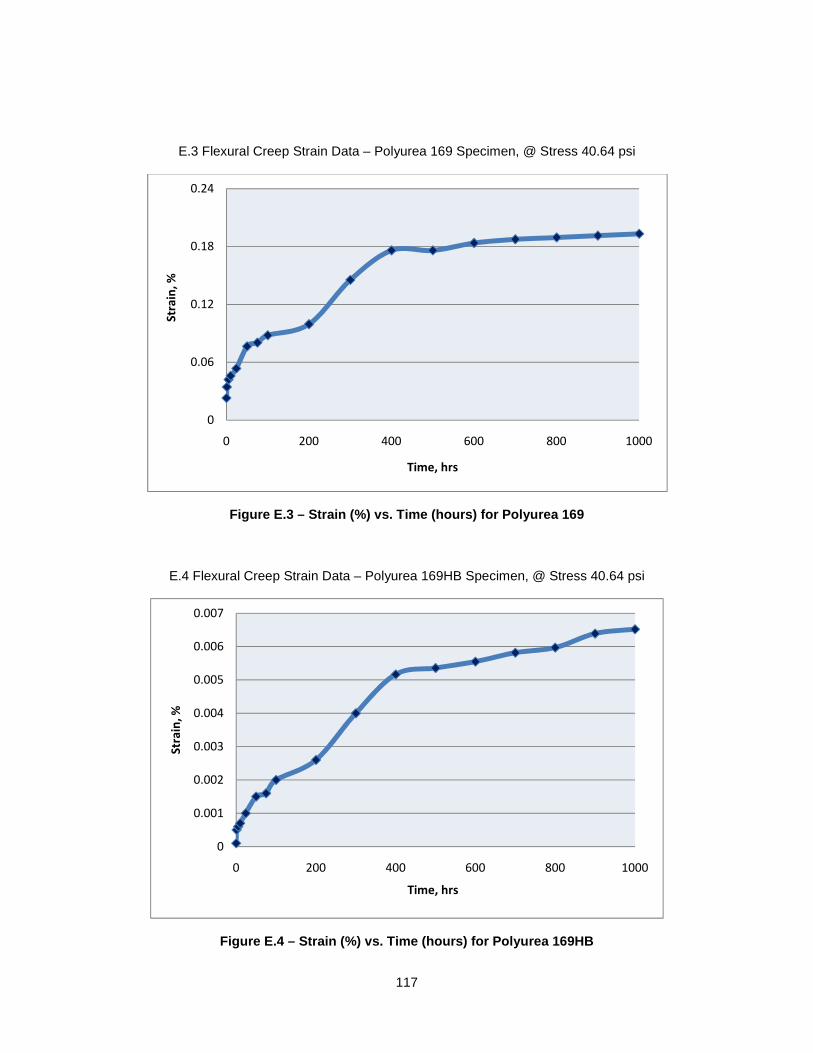
117
E.3 Flexural Creep Strain Data – Polyurea 169 Specimen, @ Stress 40.64 psi
Figure E.3 – Strain (%) vs. Time (hours) for Polyur ea 169
E.4 Flexural Creep Strain Data – Polyurea 169HB Specimen, @ Stress 40.64 psi
Figure E.4 – Strain (%) vs. Time (hours) for Polyur ea 169HB
0
0.06
0.12
0.18
0.24
0 200 400 600 800 1000
Str
ain
, %
Time, hrs
0
0.001
0.002
0.003
0.004
0.005
0.006
0.007
0 200 400 600 800 1000
Str
ain
, %
Time, hrs

118
E.5 Flexural Creep Strain Data – Polyurea 169HB Specimen, @ Stress 33.87 psi.
Figure E.5 – Strain (%) vs. Time (hours) for Polyur ea 169HB
E.6 Flexural Creep Strain Data – Polyurea 269 Specimen, @ Stress 33.87 psi
Figure E.6 – Strain (%) vs. Time (hours) for Polyur ea 269
0
0.6
1.2
0 200 400 600 800 1000
Str
ain
, %
Time, hrs
0
2
4
6
0 200 400 600 800 1000
Str
ain
, %
Time, hrs
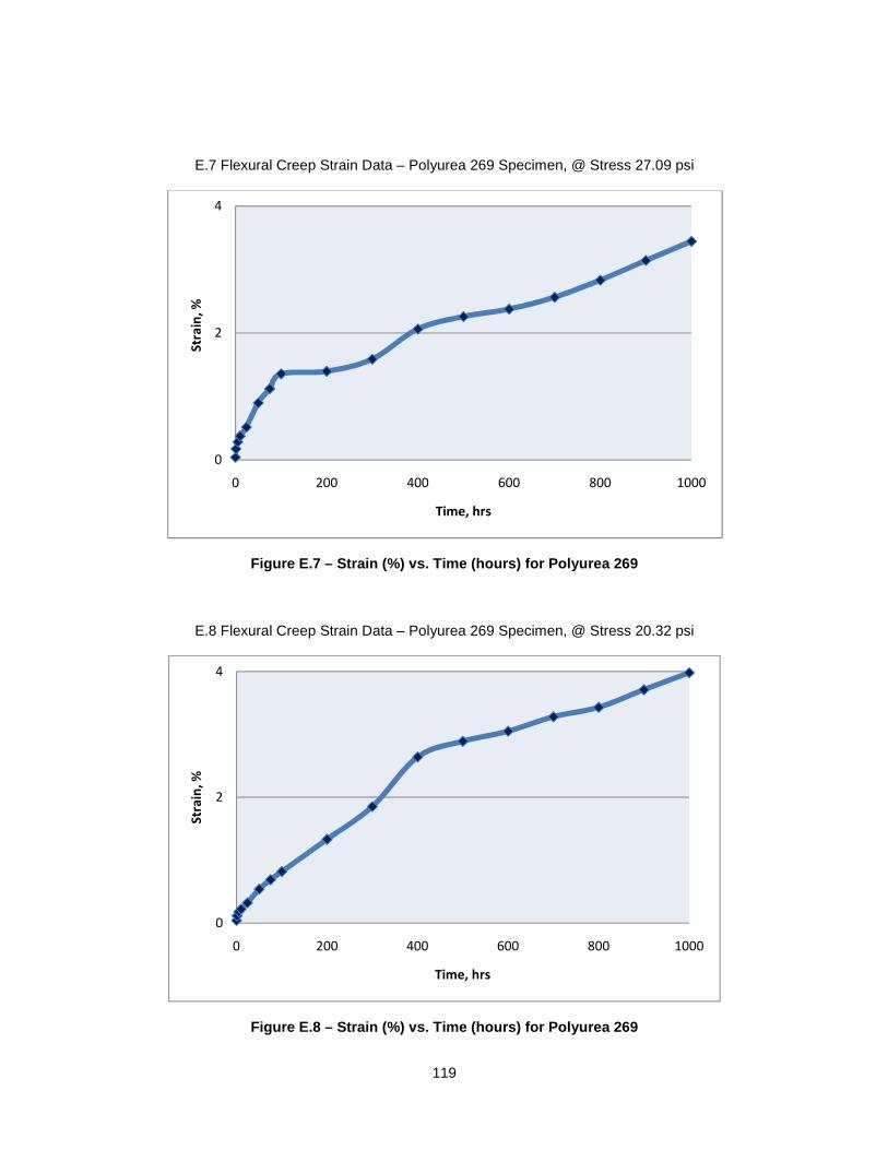
119
E.7 Flexural Creep Strain Data – Polyurea 269 Specimen, @ Stress 27.09 psi
Figure E.7 – Strain (%) vs. Time (hours) for Polyur ea 269
E.8 Flexural Creep Strain Data – Polyurea 269 Specimen, @ Stress 20.32 psi
Figure E.8 – Strain (%) vs. Time (hours) for Polyur ea 269
0
2
4
0 200 400 600 800 1000
Str
ain
, %
Time, hrs
0
2
4
0 200 400 600 800 1000
Str
ain
, %
Time, hrs
120
APPENDIX F
FLEXURAL CREEP MODULUS GRAPH
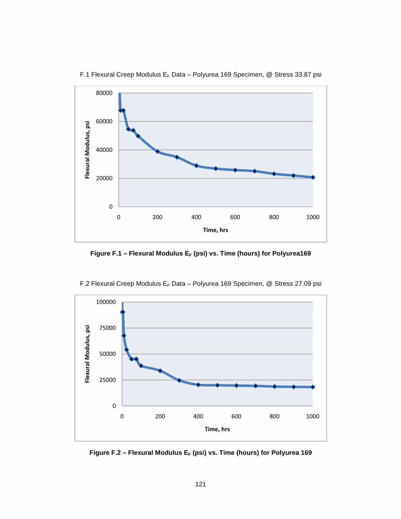
121
F.1 Flexural Creep Modulus EF Data – Polyurea 169 Specimen, @ Stress 33.87 psi
Figure F.1 – Flexural Modulus E F (psi) vs. Time (hours) for Polyurea169
F.2 Flexural Creep Modulus EF Data – Polyurea 169 Specimen, @ Stress 27.09 psi
Figure F.2 – Flexural Modulus E F (psi) vs. Time (hours) for Polyurea 169
0
20000
40000
60000
80000
0 200 400 600 800 1000
Fle
xu
ral
Mo
du
lus,
psi
Time, hrs
0
25000
50000
75000
100000
0 200 400 600 800 1000
Fle
xu
ral
Mo
du
lus,
psi
Time, hrs
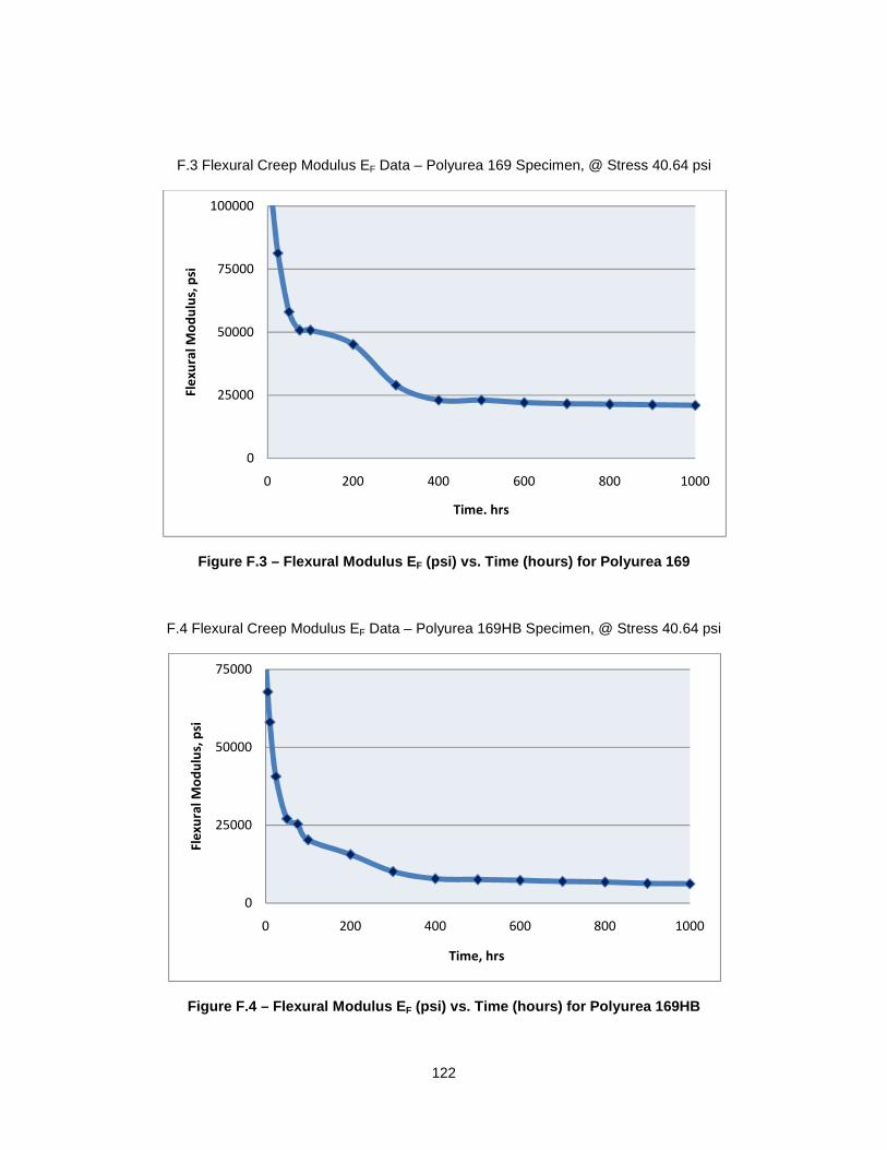
122
F.3 Flexural Creep Modulus EF Data – Polyurea 169 Specimen, @ Stress 40.64 psi
Figure F.3 – Flexural Modulus E F (psi) vs. Time (hours) for Polyurea 169
F.4 Flexural Creep Modulus EF Data – Polyurea 169HB Specimen, @ Stress 40.64 psi
Figure F.4 – Flexural Modulus E F (psi) vs. Time (hours) for Polyurea 169HB
0
25000
50000
75000
100000
0 200 400 600 800 1000
Fle
xu
ral
Mo
du
lus,
psi
Time. hrs
0
25000
50000
75000
0 200 400 600 800 1000
Fle
xu
ral
Mo
du
lus,
psi
Time, hrs

123
F.5 Flexural Creep Modulus EF Data – Polyurea 169HB Specimen, @ Stress 33.87 psi
Figure F.5 – Flexural Modulus E F (psi) vs. Time (hours) for Polyurea 169HB
F.6 Flexural Creep Modulus EF Data – Polyurea 269 Specimen, @ Stress 33.87 psi
Figure F.6 – Flexural Modulus E F (psi) vs. Time (hours) for Polyurea 269
0.00
20000.00
40000.00
0 200 400 600 800 1000
Fle
xu
ral
Mo
du
lus,
psi
Time, hrs
0
2500
5000
7500
10000
0 200 400 600 800 1000
Fle
xu
ral
Mo
du
lus,
p
si
Time, hrs
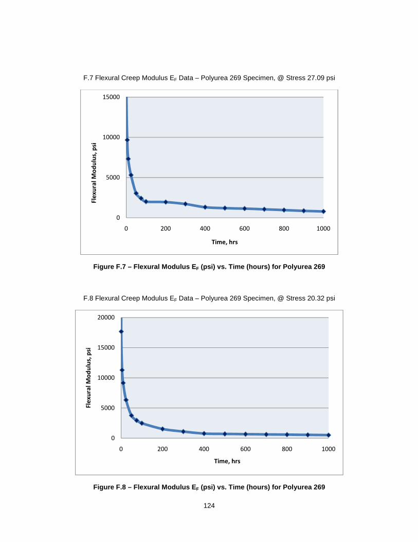
124
F.7 Flexural Creep Modulus EF Data – Polyurea 269 Specimen, @ Stress 27.09 psi
Figure F.7 – Flexural Modulus E F (psi) vs. Time (hours) for Polyurea 269
F.8 Flexural Creep Modulus EF Data – Polyurea 269 Specimen, @ Stress 20.32 psi
Figure F.8 – Flexural Modulus E F (psi) vs. Time (hours) for Polyurea 269
0
5000
10000
15000
0 200 400 600 800 1000
Fle
xu
ral
Mo
du
lus,
psi
Time, hrs
0
5000
10000
15000
20000
0 200 400 600 800 1000
Fle
xu
ral
Mo
du
lus,
psi
Time, hrs

125
APPENDIX G
LIST OF ABBREVIATIONS AND SYMBOLS
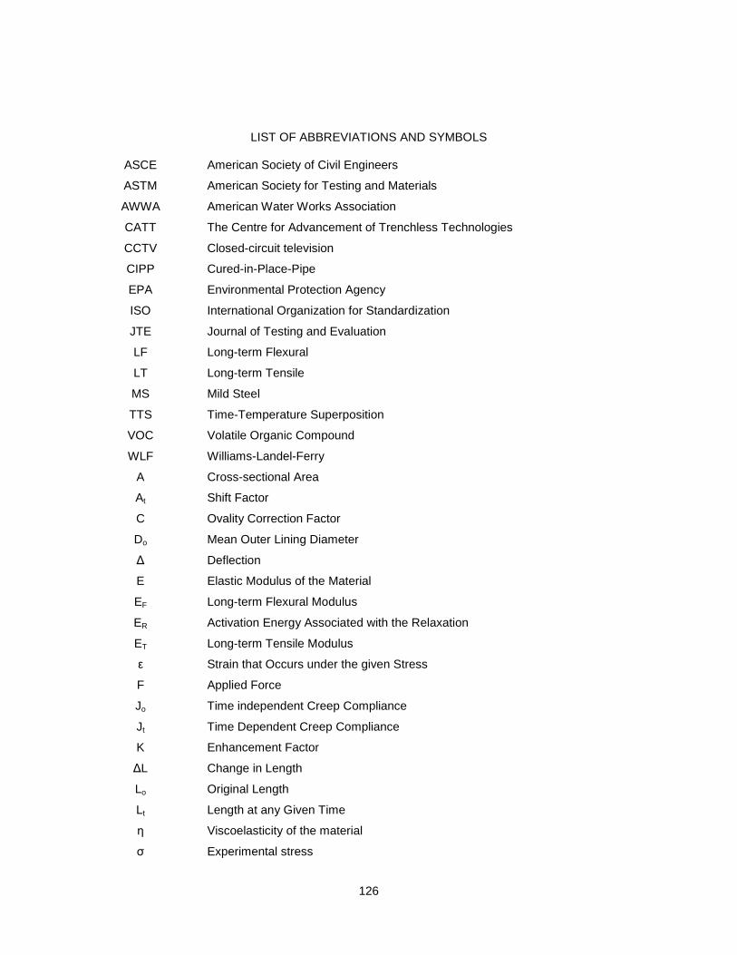
126
LIST OF ABBREVIATIONS AND SYMBOLS
ASCE American Society of Civil Engineers
ASTM American Society for Testing and Materials
AWWA American Water Works Association
CATT The Centre for Advancement of Trenchless Technologies
CCTV Closed-circuit television
CIPP Cured-in-Place-Pipe
EPA Environmental Protection Agency
ISO International Organization for Standardization
JTE Journal of Testing and Evaluation
LF Long-term Flexural
LT Long-term Tensile
MS Mild Steel
TTS Time-Temperature Superposition
VOC Volatile Organic Compound
WLF Williams-Landel-Ferry
A Cross-sectional Area
At Shift Factor
C Ovality Correction Factor
Do Mean Outer Lining Diameter
∆ Deflection
E Elastic Modulus of the Material
EF Long-term Flexural Modulus
ER Activation Energy Associated with the Relaxation
ET Long-term Tensile Modulus
ε Strain that Occurs under the given Stress
F Applied Force
Jo Time independent Creep Compliance
Jt Time Dependent Creep Compliance
K Enhancement Factor
∆L Change in Length
Lo Original Length
Lt Length at any Given Time
η Viscoelasticity of the material
σ Experimental stress
127
REFERENCES
Aktaa, J., & Schinke B. (1996) “Creep Lifetime Under Constant Load and Constant Stress: Theory and
Experiment” American Society For Testing and Materials (1996) 24(4) 212-222.
Alegre, H., J. Baptista, E. Cabrera, J. Cubillo, P. Duarte, W. Hirner, W. Merkel and R. Parena. 2006.
“Performance Indicators for Water Supply Services”. Second Edition, London: International Water
Association Publishing.
Alireza V. A., Isaacs. J., Mcgee. J., and Nematnasser. S. Primeaux II, D. J. (2004), “An Experimentally-
Based Viscoelastic Constitutive Model for Polyurea, Including Pressure and Temperature
Effects,” Polyurea Elastomer Technology: History, Chemistry & Basic Formulating Techniques.
American Society of Civil Engineers (ASCE), (2006). “Report Card for America’s Infrastructure; Drinking
Water”. American Society of Civil Engineers. Reston, VA.
American Society of Civil Engineers (ASCE) (2009). “Report Card for America’s Infrastructure.” Reston,
VA. Available at: http://www.asce.org/reportcard/2009/grades.cfm <accessed on February 2009>
ASTM F 1216 (2009), “Standard Practice for Rehabilitation of Existing Pipelines and Conduits by the
Inversion and Curing of a Resin-Impregnated Tube,” American Society for Testing Materials,
West Conshohocken, Pa.
ASTM D2990 (2009), “Standard Test Methods for Tensile, Compressive, and Flexural Creep and Creep-
Rupture of Plastics.” American Society for Testing and Materials, West Conshohocken, Pa.
ASTM D638 (2008), “Standard Test Method for Tensile Properties of Plastics.” American Society for
Testing and Materials, West Conshohocken, Pa.
ASTM D790 (2007), “Standard Test Methods for Flexural Properties of Unreinforced and Reinforced
Plastics and Electrical Insulating Materials.” American Society for Testing and Materials, West
Conshohocken, Pa.
128
AWWA (2001). “Manual of Water Supply Practices M28: Rehabilitation of Water Mains”, American Water
Works Association, Denver
AWWA (2006). “Service Life Analysis of Water Main Epoxy Lining” American Water Works Association,
Denver.
AWWA (2006). “Infrastructure Reliability: Service Life Analysis of Water Main Epoxy Lining,” American
Water Works Association, Denver.
Barbero, E., & Rangarajan, S. (2005) “Long-Term Testing Of Trenchless Pipe Liners,” American Society
for Testing and Materials (ASTM), West Conshohocken, PA.
Batra, S. (2009). “Creep Rupture and Life-Prediction of Polymer Composite,” M.S Thesis, West Virginia
University, VA, 2009.
McCrum, Buckley, and Bucknell (2003). "Principles of Polymer Engineering," 117-176.
Copon Hycote 169HB, “Technical Guidance Note: Semi Structural Polymeric Lining System,” Company
Brochure, E. Woods Company, United Kingdom. <accessed on December 2009>
Deb, A.K., Y.J. Hasit, and C. Norris. 1999. “Demonstration of Innovative Water Main Renewal
Techniques”. Denver, CO: AWWARF, AWWA.
Ding. H. Z., Wang. Z. D., Phan-Thien. N. and Reol. J (1979). “Time–Temperature Superposition Method
for Predicting the Performance of Paper by Extrapolating Accelerated Ageing Data to Ambient
Conditions” 23 (4) 451–456.
Environmental Protection Agency (EPA), 2002. “The Clean Water and Drinking Water Infrastructure Gap
Analysis”. United States Environmental Protection Agency. Washington, DC.
Ferry JD. “Viscoelastic Properties of Polymers.” Chichester: Wiley, 1980.
Findley, W. N . and Khosla. G. (1956) “An Equation for Tension Creep of Three Unfilled Thermoplastics,”
Society of Petroleum Engineers Technical Journal December 1956, 20-25.
Findley W. N, (1987) “26 Years Creep and Recovery of Poly (Vinyl Chloride) and Polyethylene,” Polymer
Engineering and Science 27(1987): 582-585.
Findley, W. N, (1944) “Creep Characteristics of Plastics,” Symposium on Plastics, American Society for
Testing and Materials (1944):18.

129
Findley, W. N., Lai, S. N., and Onaran, K. (1989). “Creep and relaxation of nonlinear viscoelastic
materials, with an introduction to linear Viscoelasticity” Dover Publications, NY.
Guan, S.W. (2003). “100% Solids Polyurethane and Polyurea Coatings Technology,” Coatings World,
pp.49-58.
Guermazi. N., Elleuch. K., Ayedi. H.K., Kapsa. Ph., Raghavan. J., and Meshii. M. (1997) “Ageing Effect
on Thermal, Mechanical and Tribological Behaviour of Polymeric Coatings Used for Pipeline
Application”, Composite Science Technology, 57, 375.
Guerrero, J.N., (1999). “Flexural Creep Analysis of Recycled Polymeric Structural Elements” PhD
Dissertation, Louisiana State University and Agriculture and Mechanical College.
Guidetti, G.P., Rigosi, G.L., Marzola, R., 1996. “The Use of Polypropylene in Pipeline Coatings.” Progress
in Organic Coating. 27, 79–85.
Harris, G.M., Lorenz, A., 1993. “New Coatings for the Corrosion Protection of Steel Pipelines and Pilings
in Severely Aggressive Environments.” Corrosion Science. 35, 1417–1423.
Heavens, J.W. (1997). “The Trenchless Renovation of Potable Water Pipelines.” Proceeding of Annual
Conference of American Water Works Association, Atlanta, GA.
ISO 899-1 (2003), “Plastics - Determination of Creep Behavior - Part 1: Tensile Creep.” International
Organization for Standardization, Geneva, Switzerland.
ISO 899-2 (2003), “Plastics - Determination of Creep Behavior - Part 2: Flexural Creep by Three-point
Loading.” International Organization for Standardization, Geneva, Switzerland.
Joachim, Markus. G., Christian. P, and W. Johannes, “Polymer Test,” 18, 257(1999).
Kamimura, T., Kishikawa, H., 1998. “Mechanism of Cathodic Disbonding of Three Polyethylene Coated
Steel Pipes.” Corrosion 54, 979–987.
Knight, M. (2005) “Evaluation of Sanexen Technologies “AQUA-PIPE” Watermain Rehabilitation Product,”
The Centre for the Advancement of Trenchless Technologies, Toronto, Canada.
Kulkarni, T., Kanchwala, M., Najafi, M., Natwig, G. and Perez, M. (2009). “Renewal of Water Distribution
Pipes using Elastomeric Polyurea Lining.” Underground Construction Technology Conference,
Tampa, Florida.
130
Lacroix, Tougui. F., Berton. A., Ranganathan. G. and Neelakantan. N. (2007). “Tensile Creep Studies on
Filled Polychloroprene Elastomer,” Journal of Testing and Evaluation (JTE) N. R. Vol 35(4), 449-
454.
Leng, A., Streckel, H., Stratmann, M., 1998a. “The Delamination of Polymeric Coatings from Steel. Part 2:
First Stage of Delamination, Effect of Type and Concentration of Cations on Delamination,
Chemical Analysis of the Interface.” Corrosion Science. 41, 579–597.
Li, R. (2000), “Time-temperature Superposition Method for Glass Transition Temperature of Plastic
Materials,” Materials Science and Engineering A278, 36–45.
Lin, H., “Creep Charaterization of CIPP Material Under Tension, Compression and Bending,” M.S Thesis,
Lousiana Tech University, LA, 1995.
Mallick, P.K (2008), “Fiber-Reinforced Composites: Materials, Manufacturing and Design,” Marcel Dekker
Inc., New York, USA.
Miller, E., and Sterrett, T. (1988). “An Evaluation of Analytical Expressions for the Representation of
Plastics Creep Data,” Journal of Elastomers and Plastics, Vol. 20(4), 346-362.
Mock.W., and Balizer.E, “Polyurea Properties and Enhancement of Structures under Dynamic Loads.”
Airlie, VA (2005).
Najafi, M., & Gokhale, S. (2005). “Trenchless Technology: Pipeline and Utility Design, Construction, and
Renewal”, New York: McGraw-Hill.
Park BD, Balatinez JJ. (1998) “Short-term Flexural Creep Behavior of Wood-fiber/Polypropylene
Composites Polymer Composites,” 19(4):377–82.
Polimerov, M. (1972). “Prediction of the Deformation and Fracture of Polymeric Material” Institute of
Polymer Mechanics, Academy of Sciences of the Latvian SSR, Riga, No. 3, pp. 498-514
Pomeroy CD. (1978) “Creep of engineering materials.” Cambridge U.K.
Primeaux II, D. J., (2000). “Polyurea Spray Coating Systems,” Primeaux Associates LLC.
Riande. E., Galleja. R. D., Prolongo. M. G., Masegosa. R. M., and Salom. C. (2000). “Polymer
Viscoelasticity Stress and Strain in Practice”, Marcel Dekker A.G, Switzerland.
131
Scotchkote 269, (2009). “Rapid Setting Polymeric Lining 269,” Design Guide for Polyurea Lining,
Company Brochure, 3M Water Infrastructure.
Scotchkote 269, (2010). “Rapid Setting Polymeric Lining 269,” Installation Guide for Polyurea Lining,
Company Brochure, 3M Water Infrastructure.
Shah, V. (1983). “Handbook for Plastics Testing Technology,” Wiley Interscience Publication, NY.
Straughan, W. T., Guice, L. K., and Mal-Duraipandian, C., "Long-Term Structural Behavior of Pipeline
Rehabilitation Systems," ASCE Journal of Infrastructure Systems, December 1995.
Thomson, W., Guice. L. K., Straughan, W.T., Norris, C.R., Bennett, R. D., and Iseley, D.T., (1996). ATTC
Report on “Long-Term Structural Behavior of Pipeline Rehabilitation Systems - Closure,” No-Dig
Engineering, Vol. 3(4).
Tobolsky, A.V. (1967) “Properties and Structure of Polymers,” Wiley, New York, pp. 144–159
Vinogradov, G.V., Malkin, A.Y. (1980) “Rheology of Polymers,” Mir, Moscow, pp. 238–248.
Williams, J. G., (1980). “Stress Analysis of Polymers,” Ellis Horwood Limited, England.
WIN (2000). “Clean and Safe Water for the 21st Century; A Renewed National Commitment to Water and
Wastewater Infrastructure,” Water Infrastructure Network. USA.

132
BIOGRAPHICAL INFORMATION
Mustafa Zakiuddin Kanchwala was born in Mumbai, Maharashtra, India on the 23th of June of 1984.
He received his Bachelors of Engineering Degree from the Mumbai University, India in May 2007. The
author had a work experience of 12 months as a project manager, and estimator in his family owned
company for interior designing. The author joined the University of Texas at Arlington in August, 2008 as
a MS candidate in Construction Management. During the course work as a graduate research assistant
under Dr. Mohammad Najafi had an opportunity to work in research project related to trenchless
technology. He has also presented technical paper for Underground Construction Technology (UCT) in
2010. For the near future the author plans to continue his research on the same topic and trenchless
technology by pursuing his PhD degree.