Suburbanization and Transportation in the

Monocentric Model

Nathaniel Baum-Snow

Department of Economics, Box B

Brown University

Providence, RI 02912-B

Nathaniel_Baum-Snow@brown.edu

Phone: 401-863-2697

Fax: 401-863-1970

November 25, 20061

1I thank Derek Neal, the editor and two referees for their many helpful comments. Inaddition, I thank Nathan Schiff for excellent research assistance. All errors are mine.

Abstract

This paper presents a version of the monocentric city model that incorporates hetero-

geneous commuting speeds by introducing radial commuting highways. This model

implies that metropolitan area population spreads out along new highways, which

are positively valued by residents. Simulations of conservative specifications of the

model imply that each additional highway ray causes about a 10 percent decline

in central city population. Given observed central population declines and urban

highway construction between 1950 and 1990, this model implies that highways can

account for an important part of urban population decentralization.

1 Introduction

One standard result from the classical monocentric land use theory developed by

Alonso [1], Muth [7] and Mills [6] is that an increase in transport speed reduces pop-

ulation density near city centers relative to suburban areas. A natural implication

of this comparative static is that improvements to the transportation infrastructure

may be an important explanation for falling urban population density. Indeed, de-

spite robust population growth in metropolitan areas, urban population density has

been declining rapidly. As documented in Baum-Snow [3], the aggregate population

in U.S. central cities as defined by their geography in 1950 declined by 17 percent

between 1950 and 1990 despite national population growth of 64 percent during this

period. This paper examines the extent to which the simple mechanism of the

monocentric city model can account for the post World War II declines in central

city populations.

I adapt a version of the standard monocentric city model to allow for heterogeneity

in commuting speeds through the introduction of radial highways. As in the standard

monocentric framework, all workers commute to a unique central location to work and

choose a residential location based on the trade-off between lost wages due to travel

time and their preference for space. The endogenously determined land rent function

distributes identical individuals over the available land such that in equilibrium,

everyone’s utility is equal and population density is decreasing in commuting time.

The implications of extending this model to allow for heterogenous travel speeds

have been explored in several ways. Some past work (as in Leroy and Sonstelie [5])

has introduced heterogeneity in commuting speed through different travel modes.

While allowing mode choice is clearly a relevant approach for a few big cities, in

only 6 metropolitan areas did at least 20 percent of the population commute by

public transportation in 1960 and by 1990 this had dropped to just one (New York).

Moreover, most previous versions of this model have symmetric or one-dimensional

space. The model developed in this paper is similar to that formulated by Anas

and Moses [2]. As in Anas & Moses’ model, this model incorporates heteroge-

neous commuting speeds through radial highways into the monocentric framework.

1

As such, equilibrium land use structure exhibits heterogeneity in residential density

conditional on distance to the city center. While more stylized than Anas & Moses’

model in some ways, the model specified in this paper generates analytical implica-

tions that apply quite generally across preference specifications and city structures.

The model also generates simulation results that are quantitatively robust to a vari-

ety of metropolitan area structures.

This paper shows that even with a conservative specification for the utility func-

tion and the commuting technology, the monocentric city model implies that new

highways are likely to be an important element needed to explain urban population

decentralization. For a metropolitan area with half of its residents living in the cen-

tral city absent any highways, simulation results indicate that the first few highway

rays each cause about a 10 percent decline in central city population, with the mar-

ginal effect declining 1 or 2 percentage points for each additional ray. Simulations

of the model yield effects of new highways that are quantiatively consistent with the

empirical results in Baum-Snow [3]. The range of simulation estimates in this paper

imply that construction of new highways can account for as much as one-third of

the decline in aggregate central city U.S. population relative to national population

growth. The mean 1950 geography central city saw its population decline by 28

percent and received about 2.5 highway rays between 1950 and 1990 implying that

highway construction can account for nearly the full decline in the population of the

average central city.

This paper proceeds as follows. Section 2 proposes the model. Section 3 proves

a few relevant analytical implications of the model. Section 4 presents some facts

about the empirical relationship between highways and suburbanization. Section

5 presents simulation results using two different utility functions and extends the

analysis to incorporate congestion. Finally, Section 6 concludes.

2 The Model

The model laid out below is a closed city absentee landlord version of the mono-

centric model in which average commuting speed differs as a function of residential

2

location. I focus on one metropolitan area that is treated as its own atomistic

general equilibrium system. There is a continuum of N individuals, each of whom

commutes to the central work location (referred to below as the CBD) and earns an

exogenously given wage w per unit time. Individuals have direct preferences over a

composite consumption good z and space s given by U(z, s). U is increasing and

weakly concave in each of its arguments and both goods are weakly normal. Because

all individuals are identical, an equilibrium consists of a situation in which every-

body has the same utility and cannot gain higher utility by moving to an alternate

residential location.

The main innovation of this model is that it incorporates highways into the trans-

portation infrastructure of a monocentric city. Highways are modelled as linear

"rays" emanating from the city’s core along which the travel speed is faster than

on surface streets. Whiles there is a discrete number of exogenously assigned rays

in the metropolitan area, a continuum of surface streets connect each point in the

metropolitan area to the central work location and to the nearest highway. Define b

as the inverse of speed on surface streets. Denote the speed ratio on surface streets

to highways as γ. Rays are distributed evenly about the origin such that they serve

the maximum number of people possible. M denotes the number of rays in the

metropolitan area. I index space in polar coordinates (r, φ), where φ is the angle to

the nearest highway ray and r is the distance to the work location.

In order to facilitate the analysis of equilibrium land use patterns, it is convenient

to break the metropolitan area up into two regions: one in which residents do not

use a highway for any part of their commutes and another whose residents commute

at least partly via a highway. In the former region, commuting time is given by br.

In the highway commuting region, one can imagine three reasonable assumptions

about how individuals access the highway using surface streets: perpendicularly via

linear streets (technology 1), around streets that form concentric circles about the

origin as in Anas & Moses [2] (technology 2) or via linear streets meeting the highway

at distances chosen to minimize total commuting time (technology 3). A general

form for the travel time from point (r, φ) to the origin that incorporates all three

3

assumptions about the commuting technology is breL(φ) where1eL(φ) = γ cosφ+ sinφ given technology (1)(1)

= γ + φ given technology (2)

= γ cosφ+p1− γ2 sinφ given technology (3)

Individuals living at each location (r, φ) choose the commuting route to minimize

total travel times. As such, the minimum time it takes to travel to the center (0, 0)

from (r, φ) is given by:

(2) L(r, φ) = min[br, breL(φ)]Define φ as the angle separating the zone in which individuals use a highway for part

of their commutes and that in which they commute directly downtown on surface

streets or use an adjacent highway:

(3) φ = min[solution to eL(φ) = 1, πM]

If there are sufficiently few highways such that some commute only on surface streets,

1The expression for eL(φ) given commuting technology (3) is derived as follows. Using the lawof cosines, the optimal choice of CBD distance x at which to access the highway is the result of theminimization problem:

minx[bγx+ b

pr2 + x2 − 2xr cosφ]

The first-order condition implies a quadratic equation in x that when solved implies

x∗ = 2r(1− γ2) cosφ±

pcos2 φ(γ2 − 1)2 − (1− γ2)(cos2 φ− γ2)

1− γ2

Simplifying the expression under the square root and using the fact that x∗ < r cosφ, this becomes

x∗ = r(1− γ2) cosφ− γ sinφ

p1− γ2

1− γ2

= r(cosφ− γp1− γ2

sinφ)

Inserting this expression into the commuting time function above and simplifying yields theclaimed result.

4

commuters living along the ray formed by the angle φ are indifferent between using

a highway for part of their commutes and surface streets exclusively. If there are

enough rays such that everybody uses a highway, φ is the angle at which individuals

are indifferent between using adjacent highways for part of their commutes. If

γ = 0.5 and the commuting route uses linear surface streets perpendicular to the

highway (technology 1), there exist people who do not use a highway for any part of

their commutes for M < 5. I set the pecuniary cost of commuting to 0.2

Given one of these potential commuting technologies, the spatial distribution of

residences is determined by utility maximization subject to time and budget con-

straints. I normalize individuals’ total time endowment to 1 such that all time is

spent either working or commuting. The price of land is given by R(r, φ) and the

price of the consumption good is normalized to 1. As such, the following equation

represents each individuals’ resource constraint conditional on living at point (r, φ):

(4) z +R(r, φ)s = w[1− L(r, φ)]

R(r, φ) is determined endogenously as described in Section 3 below. I denote the

compensated demand functions for the composite good and space as ez(R, u) andes(R, u) respectively. I denote the distance from the central business district to the

border between the central city and the suburbs as rc. This variable is exogenously

determined and will serve only to define boundaries within which to evaluate popu-

lation decline as highway rays are added to the metropolitan area.

The bid-rent function for space is defined as the maximum an individual would

be willing to pay to reside at location (r, φ) given utility level u. It can be derived by

solving for R(r, φ) from Equation (4) and imposing that each consumer is maximizing

over s and z subject to achieving utility level u.

(5) ψ[L(r, φ), u] = maxs

½w[1− L(r, φ)]− Z(s, u)

s

¾2As long as pecuniary travel cost is an increasing linear function of L(r, φ), its exclusion does

not affect the qualitative urban form implied by this model. Provided the wage is high enoughthat pecuniary travel cost is a small fraction of income, it does not matter quantitatively either.

5

Z(s, u) is achieved by inverting the equation U(z, s) = u to solve for z. Differen-

tiating Equation (5) reveals that bid-rent is decreasing and convex in travel time

from the city center. Bid-rent functions are a convenient definition that will be used

extensively in the next section to examine how equilibrium land use patterns change

with the introduction of rays.

3 Equilibrium Land Use and Highways

This model retains the primary standard results of the classic monocentric city model,

except that the uniform linear correspondence between travel time and distance to

the center is broken. Indeed, if space is indexed in terms of travel time rather than

distance to the center, this model maps exactly into the classical land use model.

Since all individuals are identical, equilibrium land rent at each populated location

equals bid-rent given the equilibrium level of utility. The equilibrium land use

pattern in the metropolitan area is thus determined jointly by the demand function

for space, a condition stating everyone has a place to live and an equation that

equalizes rent at the edge of the populated area to rural land rent. I denote uM as

the equilibrium level of utility given M rays in the metropolitan area.

Metropolitan areas are large enough to accommodate the mass of N individuals

with the urban fringe rMf (φ) endogenously determined by equating equilibrium bid-

rent with the market rental rate for rural land at all angles. At angles φ ≥ φ,

Equation (6) determines the distance to the fringe that I denote as rMf :

(6) ψ(brMf , uM) =w[1− brMf ]− Z(es(Ra, u

M), uM)es(Ra, uM)= Ra

Similarly, at angles φ ≤ φ, bid-rent for residential land must equal rural land rent.

Because all individuals at the fringe face the same rental rate of land Ra and have

the same utility uM , it is evident that they also must have the same commuting time.

6

Equilibrium fringe distance is therefore given by the following function:

rMf (φ) =rMfeL(φ) if 0 ≤ φ ≤ φ(7)

= rMf if φ ≥ φ

This function provides the upper limit of integration in the market clearing condition

for space below.

Each ray influences commuting time only in the wedge bounded by angle φ on

either side of it. In the remaining land within the angle 2π−2Mφ, commuting time

is not affected by rays. Define the function q(·) to solve (6) such that rMf = q(uM).

Substitution of the demand function and the rearranged fringe rent function into the

market clearing condition for space yields:

N = 2M

φZ0

q(uM )

L(φ)Z0

rdrdφes[ψ(breL(φ), uM), uM ]+(2π − 2Mφ)

q(uM )Z0

rdres[ψ(br, uM), uM ](8)

Equation (8) determines the equilibrium utility level uM in the city. Fujita’s [4]

discussion of existence and uniqueness of the equilibrium applies exactly with the

replacement of distance to the center with travel time.

Figure 1 presents a schematic diagram of the spatial structure of the city and

what happens to urban form when a new ray is introduced. A new highway ray

represents a decline in commuting time for a sector of the metropolitan area. This

elicits two effects. First, the price of land decreases because more land is accessible

for each given commuting time. Holding the agricultural land rent Ra constant, this

means that for φ > φ, the fringe moves in towards the center. The decrease in land

rent causes agents to increase land consumption via a price effect, inevitably pushing

some people further from the center and lowering population density as a result.

7

Second, average net income rises, causing people to consume more land (assuming

land is normal) through a wealth effect, also pushing them away from the center.

Since people consume more of both space and the composite consumption good, the

new highway causes the equilibrium utility level in the city to rise. In addition, the

highway causes the residential land area of the metropolitan area to rise.

Proposition 1 formalizes these results. It states that an additional ray always

causes (i) equilibrium utility in the metropolitan area to rise, (ii) the portion of the

urban fringe in a region where nobody uses the highway for part of her commute to

move inwards and (iii) the portion of the urban fringe on the new highway ray to

move outward.

Proposition 1. If M 0 =M + 1 then in equilibrium

i) uM0> uM ii) rM

0f < rMf iii)

rM0

f

γ> rMf

Proof See Appendix A.

An intuitive way to see the structure of different urban equilibria with highways

is through examination of bid-rent functions. Indeed, bid-rent and population den-

sity are proportional assuming several standard specifications of the utility function.

Figure 2 shows how the changing shape of the bid-rent function implies the different

city structures in 0, 1 and 2 ray environments. Each line in the figure is a bid-rent

function conditional on the angle to the nearest ray and the number of rays in the

metropolitan area. The first argument gives the travel time to the work location

and the second argument gives the equilibrium utility level. The travel time of rb

indicates that the bid-rent function is relevant for φ > φ while the travel time γrb

indicates that the bid-rent function is relevant for φ = 0. The superscripts on u and

rf give the number of rays in the metropolitan area.

As is a standard result from monocentric theory, an increase in the utility level

in the city is associated with a decline in bid-rent for the same travel speed. This

increase in utility associated with extra rays causes the bid-rent function to shift

down and intersect Ra at a distance that is closer to the CBD. Given a utility level

uM , all bid-rents conditional on φ are the same at the center since travel time is equal

8

at 0. As seen in Figure 2, as φ increases from 0 to φ, the bid-rent function gets

steeper, representing the increased relative value individuals place on being near the

CBD due to the lower average commuting speed. Bid-rent along the ray intersects

Ra at a distance exceeding the fringe absent the ray. This reflects the fact that

in order to house the full population, some extra space has to be claimed along the

highway.

While the average population density in the metropolitan area declines with new

highways, one area sees increased population density. Individuals move to live

near the new ray and enjoy shorter commuting times. As such, an area near the

urban fringe and near the highway sees increased population density as a result of

the new highway. To see that population density increases near the highway but

decreases elsewhere, it is instructive to compare population densities in the 0 and 1

ray equilibria at the coordinates (r1f , φ) and (ε, 0) as examples. To simplify notation,

define sM(r, φ) ≡ es(ψ(L(r, φ), uM), uM). At (r1f , φ), income net of commuting cost

does not change with the introduction of the ray, yet utility of the metropolitan area

goes up. Therefore, consumption of space increases through a pure price effect:

1

s1(r1f , φ)<

1

s0(r1f , φ)

In addition, note that for ε arbitrarily small,

(9)1

s1(ε, 0)<

1

s0(ε, 0)

because the general equilibrium effect of the highway reducing rents overwhelms

the marginal commuting time reduction associated with using the highway for a

very short commute. That is, inequality (9) holds because from Proposition 1,

u1 > u0 and ψu < 0, but commuting cost declines only marginally, implying that

ψ(εγb, u1) < ψ(εb, u0). Therefore, demand for space increases at all angles for a

sufficiently small radius through a price effect. In addition, commuting time at (ε, 0)

falls slightly causing income net of commuting cost to rise. Demand for space near

the new highway therefore also increases through an income effect. This increase in

9

per-capita space consumption implies a decline in population density. Thus if rc is

sufficiently small, central city population is assured to decline with each new highway

ray. This result makes up the main argument in the proof of Proposition 2.

Proposition 2. ForM 0 =M+1 and rc sufficiently small, population of the central city assuming

M 0 rays is less than population of the central city assuming M rays.

Proof Central city population is given by:

Nc = 2M

φZ0

rcZ0

rdrdφes[ψ(breL(φ), uM), uM ]+(2π − 2Mφ)

rcZ0

rdres[ψ(br, uM), uM ](10)

From Proposition 1, u is increasing in M . Using the inequalities ψu <

0, ∂s∂R

< 0 and ∂s∂u

> 0, it must be that 1s[ψ(br,uM0),uM0 ]

< 1s[ψ(br,uM ),uM ]

for all

r > 0.

Define r∗(φ) to solve ψ(breL(φ), uM 0) = ψ(br, uM). As in the argument made

for the proof to Proposition 1 part iii, in the range r ∈ [0, r∗(φ))Xφ ∈ [0, φ),

1es[ψ(breL(φ), uM 0), uM 0 ]<

1es[ψ(br, uM), uM ]Since at all angles from the center population density falls at some radius,

population density falls in the entire region near the center of the city for an

increase in rays.

4 Empirical Observations

In a companion paper, Baum-Snow [3] empirically investigates the extent to which

highway construction caused suburbanization in the United States between 1950

10

and 1990. In that paper, I use variation across metropolitan areas in the number

of highways in a 1947 plan of the national highway system as a source of plausibly

exogenous variation in the number of highways actually received. I find that each ray

causes approximately a 10 percent decline in central city population, ceteris paribus.

When added up, highway construction empirically accounts for about one-third of

the gap between metropolitan area population growth and central city population

growth between 1950 and 1990.

Table 1 explores the empirical relationship between population decentralization

and highway construction. Elements in Table 1 represent the average fraction of

metropolitan area residents living central cities as defined by their 1950 geography

in 1950 and 1990 as a function of the number of highways rays built to serve central

business districts over this period. Panel A includes all metropolitan areas with at

least 100,000 residents with central cities of at least 50,000 residents in 1950. Panel

B limits the sample only to include metropolitan areas with central cities that are

at least 20 miles from the nearest coast, lake shore or international border. I break

out data for the more select sample because these metropolitan areas have structures

that are most similar to that of the theoretical metropolitan area considered in this

paper.

The average fraction of the population living in central cities fell from about 50

percent to about 25 percent between 1950 and 1990. Table 1 shows that highway

construction is associated with this decline. As measured in shares, both panels show

decreasing monotonic relationships between the decline in central city population

share and new highways between 3 and 7 rays. When measured in logs, the more

select sample in Panel B produces a weakly monotonic relationship between 1 and

7 rays.3 The relationship reported in Panel B implies that the average effect of one

ray is associated with a decline in log central city population share of approximately

0.07 if 0 rays are included and 0.10 if 0 rays are excluded4. The more thorough

3The anomaly at 0 rays exists primarily because cities that received 0 rays are smaller geograph-ically than other cities. When the small size is controlled for in regressions, the anomaly largelydisappears.

4These average rates of decline are the coeffiicients on ∆ray in a simple regression of ∆ log(Nc

N )on ∆ray. Both coefficients are significant at the 5 percent level.

11

empirical analysis in Baum-Snow [3] shows that these descriptive results hold up to

causal scrutiny. These numbers are similar in magnitude to the model simulation

results presented in the next section.

5 Simulations

Sections 2 and 3 develop a mechanism by which new highway rays cause declines in

urban population density in the context of a monocentric model. Further restrictions

on the model are required to determine the magnitude of these declines. This section

addresses this question through simulation. It is important to note that the model

specified in this paper is developed in order to facilitate simulation. The model’s

parsimony means that only a few parameters need be chosen for simulation. For all

simulations, I use commuting technology (1), in which commuters must access the

highway using a perpendicular surface street. This technology limits the influence

of new highways on central population decline more than any other technology in

which travel only along straight lines is possible. As such, with an appropriate

specification of preferences, these simulation results represent a near lower bound on

the effect of highways on central city population as implied by this model. After

presenting results from simulating the model, I extend the analysis to incorporate

congestion.

5.1 Basic Results

I focus primarily on simulation examples using the utility function U = z + α ln(s).

Quasilinear utility is a convenient preference specification for two reasons. First,

the quasilinear utility function’s income elasticity of demand for space of 0 limits the

response of population density to faster transportation infrastructure to be driven

only by a price effect. Second, quasilinear utility is convenient because results are

very stable over a wide range of values for the shape parameter of the utility function,

the wage, base travel speed and metropolitan area population.

Numerical calculation of equilibria requires choosing elements of the parameter

12

vector (N,w, b, γ, α,Ra,M). Table 2 shows how several outcomes of interest change

as a function of rays given metropolitan area populations of 100 thousand (Panel

A) and 1 million (Panel B). Central city radius rc is chosen such that in the 0 ray

equilibrium, half of the population lives in the central city. This fraction is near the

mean across metropolitan areas in the data from 1950. The other parameters are

chosen to mimic conditions seen in modern U.S. metropolitan areas. A wage of 100

is chosen to represent $10 an hour in a 10 hour day. Travel speed is chosen to be

30 mph on city streets and 60 mph on highways, implying a b of 1300

and γ of 0.5.

The utility function’s shape parameter α is chosen as 0.3. Finally, rural rent Ra is

chosen to be 1.

Given the patterns of urban decentralization documented in Table 1, one statistic

of interest is the evolution of central city population as a function of the number of

rays. Solving for central city population can be reduced to two steps: solving for

rMf from the implicit function in Equation (11) and inserting the result back into the

expression for Nc, which in general is given by Equation (10).5

(11) N =Ra

αewαbrMf (

wb

α)−2

⎡⎣ (wbα)22M

R φ0

R rMfγ cosφ+sinφ

0 re−wαrbL(φ)drdφ

+(2π − 2Mφ)[1− e−rMf wb/α − rMf

wbαe−r

Mf wb/α]

⎤⎦As is shown below, the evolution of central city population in response to new rays

is quite stable across parameter values.

Table 2 Panels A and B track central city population, fringe distance not near a

ray (rMf ), utility and rent at the origin as a function of the number of rays given small

and large metropolitan area populations. Both panels show central city population,

fringe distance, and central rent declining and utility increasing in the number of

rays. The marginal effect of each additional ray on all of these variables declines

in absolute value in the number of rays. Note that only central city population

depends on the choice of rc.

Taking central city population in the 0 ray equilibrium as given, Panel C traces

out the evolution of the change in central city population as a function of the number

5All calculations relevant for the simulations are available upon request from the author.

13

of rays. Each row shows the effect on central city population of each marginal ray,

holding the radius of the central city fixed. The central city radius is determined

by the fraction of metropolitan area population assumed to reside in the central city

listed in the left-most column. Results in Table 1 Panel C show that the first ray

causes the log central city population to fall by 0.11, with the fall in central city

population declining 1-2 percentage points for each additional ray. The percent

decline in central city population falls with increases in central city population share

in the 0 ray equilibrium and equivalently with increases in the central city radius.

Table 3 presents simulation results analogous to those in Table 2 using the Cobb-

Douglas utility function. Each of the parameters is the same, with space given a

30 percent budget share. Note that since Cobb-Douglas has an income elasticity of

demand for space of 1, the amount of space consumed by the metropolitan area is

much greater. As such, the rent at the origin is much lower than in the quasilinear

utility case reported in Table 2. Despite these differences in levels, the profile of the

changes as a function of the number of rays is very similar for the two specifications

of the utility function.

Table 3 Panel C presents the profile of central city population as a function of

the number of rays. These results show effects within 0.04 greater in absolute value

of those implied by quasilinear utility. A metropolitan area with half its population

in the central city lose about 13 percent of its population for the first ray, 11 percent

for the second ray and 9 percent for the third ray. This effect declines by about 1

percentage point for each additional ray thereafter.6

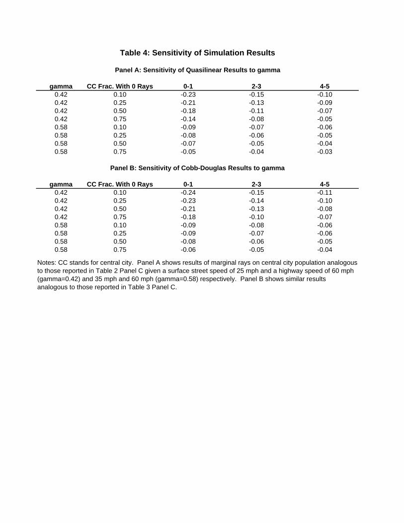
Table 4 explores the sensitivity of the central city population results to the choice

of speeds on highways to city streets. Table 4 Panel A replicates the simulation

results for the profile of central city population reported in Table 2 Panel C assuming

speed ratios on surface streets to highways of 2560and 35

60instead of 30

60. These results

show that the magnitudes of the marginal effects are decreasing in the speed ratio.

Given a speed ratio of 2560, the first few rays cause 18, 14 and 11 percent central city

6Simulation results using the Anas-Moses [2] commuting technology in which highway users musttravel around a circle centered at the CBD to access a highway give effects within 0.02 smaller inmagnitude than those reported in Tables 2 and 3 Panel C.

14

population declines respectively. Given a speed ratio of 3560, the first few rays cause

7, 6 and 5 percent declines respectively. Panel B similarly replicates results based

on Cobb-Douglas preferences, yielding marginal effects on central city population of

21, 16 and 13 percent given the low speed ratio and 8, 7 and 6 percent given the

high speed ratio. Marginal effects of only the first, third and fifth rays are reported

to maintain parsimony in the table.

In addition to examining the sensitivity of simulation results to travel speeds, I

also explored the extent to which the results presented in Tables 2 and 3 Panel C

are sensitive to the wage, metropolitan area population and the shape parameter

of the utility functions. I simulated the model for all shape parameters between

0.1 and 0.9, for population levels up to 10 million and for wage rates down to 50.

In no case do any numbers in Table 2 Panel C change by more than 0.03 nor do

numbers in Table 3 Panel C change by more than 0.05. The largest changes for the

Cobb-Douglas utility case occur when space is given a budget share of 0.9 and the

metropolitan area population is at least 5 million.

5.2 Adding Congestion

The model presented in Sections 2 and 3 assumes that the transport infrastructure

is not congestible. In this subsection, I extend the model to handle congestion in a

simple way and present associated simulation results. I relegate the consideration

of congestion to an extension of the model presented in Sections 2 and 3 for two

reasons. First, the existence of congestion means that the simulation results from

the previous subsection will no longer be insensitive to metropolitan area population.

Second, empirically congestion did not start to become a major source of commuting

time loss until the 1990s.

A straightforward way of extending the analysis to incorporate congestion, similar

to that employed by Anas and Moses [2], is to make γ an increasing function of the

15

population affected by a highway:

γ = f(

Z φ

0

Z rMf

L(φ)

0

rdrdφes[ψ(breL(φ), uM), uM ])(12)

f 0 ≥ 0

Denote γM to be the equilibrium value of γ given M rays. Congestion represents

another force pushing population density up near the center of the city in response

to an increase in N because dNc

dγ> 0 and df

dN> 0. Similarly, this formulation

of congestion implies that ceteris paribus, more rays lead to a weak decline in the

equilibrium value of γ because they induce some highway users to move from using

other rays, thereby reducing the population around each ray. Thus holding the

number of lanes constant, the effect of the first ray on central city population is

smaller than it would be without congestion. The effect of the second ray is larger

than it would be if γ were fixed at γ1 because the next ray causes γ to fall to γ2. The

parameterization of the function f and the profiles of the price and wealth effects of

demand for space as a function of γ determine whether the response of central city

population to the second ray in a world with congestion is less or greater than in a

world without congestion.7

I evaluate the potential importance of congestion by simulating the model allow-

ing γ to be determined by the equilibrium population using the highway. I take the

formula for speed on congested highways from the Texas Transportation Institute’s

(TTI) 2004 Mobility Report [8] and adapt it slightly to fit this context.8 The formula

is estimated by the TTI based on data taken from sampled portions of the highway

network. It is piecewise linear and weakly monotonic in average daily traffic. Equi-

librium highway travel speed is 60 mph at traffic levels below 13,260 vehicles per lane

7Vickrey [9] proposes a more complicated formulation which in the context of this model wouldmanifest itself as a "flow congestion" term in the travel time function: L(r, φ) = min[br, br(γ cosφ+

sinφ) + λR r cosφ0

³N(v)t(v)

´kdv] where N(v) is the number of commuters using the highway between

v and the edge of the MSA and t is the throughput of the highway.8I alter the TTI’s congestion function in order to make it monotonic. Details are in Appendix

Table 1.

16

per day, with the equilibrium speed dropping to 30 mph by 72,000 vehicles per lane

per day. The formula used is reported in Appendix Table 1. For the simulations,

I assume that each new highway is 4 lanes in each direction and that 2 individuals

commute together in each vehicle. Given that only about half the U.S. population

commutes to work outside the home, the 2 person per car assumption allows the

model to better capture commuting patterns for observed population levels.

Unlike the results presented in the previous subsection, simulation results incor-

porating congestion are sensitive to the population of the metropolitan area. Table

5 presents simulation results with γ endogenized to account for the number of road

users according to the formula detailed in Appendix Table 1. Numbers in Table

5 are calculated using the same parameter values as are used for Table 2 except

population. With this formulation of the congestion function and transportation

infrastructure, congestion starts to reduce travel speeds when the metropolitan area

reaches about 500,000 people. As such, Panel A reports simulation results for a

metropolitan area of this size. Panel A shows that congestion reduces the reduction

in central city population caused by the first ray by up to 4 percentage points. Five

rays is enough infrastructure to eliminate all congestion in this case.

Table 5 Panel B reports results for a metropolitan area of 1 million inhabitants.

A metropolitan area of 1 million inhabitants with half its population in the central

city in the 0 ray equilibrium sees central city population drop by 3 percent for the

first ray, 4 percent for the second, third and fourth rays and 5 percent for the fifth

ray. At 10 rays, the spatial distribution of the population looks the same as in the

uncongested case because there is enough transportation infrastructure to bring γ

back to its uncongested value.

Data collected by the Texas Transportation Institute indicates that congestion is

not likely to be a major force mitigating highways’ influence on changing residential

land use patterns since 1950. Among the 139 largest metropolitan areas in 1950,

the average ratio of free-flow to congested traffic speeds on limited access highways

was 1.16 in 1990. Therefore, it appears that communities built up their highway

infrastructure almost sufficiently to fulfill the increased travel demand associated

with their rising and decentralizing populations.

17

6 Conclusions

This paper proposes a land use and commuting model that incorporates radial high-

ways. I show that new highways affect urban form by causing the population to

spread out along the highways. In addition, holding the population of the metropol-

itan area constant, the urban fringe in areas not near the highway moves inwards.

This simple model implies that highway construction may have contributed markedly

to the dramatic change in urban land use patterns observed between 1950 and 1990

in the United States. Results from simulating the model imply that indeed new high-

ways are likely to have had a sizable impact on central city populations. Applying

the simulation results in Table 2 Panel C to observed average highway construc-

tion of about 2.5 rays per metropolitan area, counterfactual central city population

estimates imply that nearly the full decline of 28 percent in average central city pop-

ulation can be explained by highway construction. Descriptive evidence using data

from 139 metropolitan areas reveals changes in observed central city population as

a function of highway construction that is similar to that implied by the simulation

results.

While the mechanism proposed here produces qualitative and quantitative results

that are quite robust, the model used is highly stylized. Indeed, casual empirical

observation reveals that employment decentralization has occurred apace with res-

idential decentralization, a phenomenon that is ignored by the model in this pa-

per. While others have proposed models that endogenize employment location,

these models have few general analytical comparative static implications. As such,

it is valuable to understand the extent to which a simple tractable model featuring

highway construction can explain suburbanization.

18

A Proof of Proposition 1

If M 0 =M + 1 then in equilibrium

i) uM0> uM : Compare a city with 0 rays and 1 ray. The market clearing

condition for space (Equation 8 in the text) implies that

0 = 2

φZ0

q(u1)

L(φ)Z0

rdrdφes[ψ(breL(φ), u1), u1]+(2π − 2φ)

q(u1)Z0

rdres[ψ(br, u1), u1] − 2πq(u0)Z0

rdres[ψ(br, u0), u0](13)

Recall that q(·) gives the equilibrium fringe distance far from highways through

solving the fringe rent condition (Equation 6 in the text) for rMf . Suppose that u0 >

u1. I prove by contradiction that utility cannot be decreasing inM . Using Equation

(6), the Implicit Function Theorem and the Envelope Theorem, drfdu= −−

∂z(s,u)∂u

−wb < 0

so q(u1) > q(u0). Using the fact that space is a normal good, es[ψ(L(r, φ), u1), u1] <es[ψ(L(r, φ), u0), u0]. These two conditions imply that(14) 2π

⎡⎢⎣ q(u1)Z0

rdres[ψ(br, u1), u1] −q(u0)Z0

rdres[ψ(br, u0), u0]⎤⎥⎦ > 0

and applying Equation (14) to (13) we have

(15)

φZ0

q(u1)

L(φ)Z0

rdrdφes[ψ(breL(φ), u1), u1] < φ

q(u1)Z0

rdres[ψ(br, u1), u1]

19

But

φ

q(u1)Z0

rdres[ψ(br, u1), u1] =

φZ0

q(u1)Z0

rdrdφes[ψ(br, u1), u1]<

φZ0

q(u1)

L(φ)Z0

rdrdφes[ψ(br, u1), u1]<

φZ0

q(u1)

L(φ)Z0

rdrdφes[ψ(breL(φ), u1), u1]which contradicts (15). Thus, it must be that u1 > u0. An analogous argument

follows for all M > 0.

ii) rM 0f < rMf : To understand how equilibrium land use changes with M, we must

first understand how the equilibrium land rent function changes with M. We can

express land rent in terms of the bid-rent function:

(16) ψ(L(r, φ), u) = maxs

½w[1− L(r, φ)]− Z(s, u)

s

¾Using the envelope theorem, ∂ψ

∂u< 0. Thus given result i, areas of the city with

no change in travel times see land rents fall with M . Therefore, since Ra does not

change, fringe distance in these same areas also falls with M .

iii)rM

0f

γ> rMf : Once again, consider the case of moving from a regime with 0 rays

to a regime with 1 ray. Result i states that utility rises with M and ii) shows that

equilibrium land rent falls with M for φ > φ. Thus since space is a normal good,es[ψ(L(r, φ), u1), u1] > es[ψ(L(r, φ), u0), u0] in the region φ > φ. Also note from result

ii that ψ(0, u1) < ψ(0, u0).

To examine the φ < φ region, it is instructive to think about the shape of the

bid-rent function for land in the 0-ray equilibrium compared to that in the 1-ray

equilibrium at φ ≥ φ and φ = 0. The derivative of the rent function as a function of

20

r is:

(17) ψr = −wmin[b, beL(φ)]es[ψ(L(r, φ), u), u]

The rent function is thus less steep in the region φ < φ than in the remainder of

the metropolitan area. Further, the rent function at all points is less steep in the

1-ray equilibrium than the 0-ray equilibrium. Define r∗(φ) to solve ψ(rbeL(φ), u1) =ψ(rb, u0) for the region ψ(rb, u0) > Ra. Given the normality of land and the fact

that the fringe distance is the furthest from the center at φ = 0, it must also be true

that for r ≤ r∗(φ), s1(r, φ) > s0(r, φ). Using the market clearing condition for space

and the result that r1f < r0f :

N − (2π − 2φ)r0fZ0

rdres[ψ(br, u0), u0] − 2φZ0

r∗(φ)Z0

rdrdφes[ψ(br, u0), u0]> N − (2π − 2φ)

r1fZ0

rdres[ψ(br, u1), u1] − 2φZ0

r∗(φ)Z0

rdrdφes[ψ(breL(φ), u1), u1]or

2

φZ0

r1f

L(φ)Zr∗(φ)

rdrdφes[ψ(breL(φ), u1), u1] > 2φZ0

r0fZr∗(φ)

rdrdφes[ψ(br, u0), u0]That is, there remain more people to be housed in the region r ∈ [r∗(φ),∞) Xφ ∈ (0, φ) in the 1-ray equilibrium than the 0-ray equilibrium. r∗(φ) must exist

for some φ, otherwise not everybody could be housed in the 1-ray equilibrium. By

definition of r∗ and the fact that ψr(bγr, u1) > ψr(br, u

0), rent must be greater in

the 1-ray equilibrium than the 0-ray equilibrium in the region r > r∗(φ). Because

Ra is the same in both equilibria, the extent of the city at φ = 0 must be greater

in the 1-ray equilibrium than the 0-ray equilibrium. The same argument follows for

all M > 0. Q.E.D.

21

References

[1] W. Alonso. Location and Land Use. Harvard University Press, Cambridge, 1964.

[2] A. Anas, L. Moses. Mode choice, transport structure and urban land use. Journal

of Urban Economics, 6(2):228—246, 1979.

[3] N. Baum-Snow. Did highways cause suburbanization? Quarterly Journal of Eco-

nomics, forthcoming.

[4] M. Fujita. Urban Economic Theory: Land Use and City Size. Cambridge Univer-

sity Press, Cambridge, 1989.

[5] S. F. Leroy, J. Sonstelie. Paradise lost and regained: Transportation innovation,

income, and residential location. Journal of Urban Economics, 13(1):67—89,

1983.

[6] E. S. Mills. An aggregative model of resource allocation in a metropolitan area.

American Economic Review, 57(2):197—210, 1967.

[7] R. F. Muth. Cities and Housing. University of Chicago Press, Chicago, 1969.

[8] D. Schrank, T. Lomax. The 2004 Urban Mobility Report. Texas Transportation

Institute, tti.tamu.edu, 2004.

[9] W. S. Vickrey. Congestion theory and transport investment. American Economic

Review, 59(2):251—260, 1969.

22

highway ray

rc

Figure 1: The Effect on Urban Form of a New Ray

φ

examplecommute

CBD

fr 1

fr 0

φφγ sincos

1

+fr

Figure 2Graphical Depiction of Rent Functions in 0, 1 and 2 Ray Equilibria

ψ(rb,u0)

ψ(rb,u1)

ψ(γrb,u1)

r1frγ

0fr

1fr

Ra

R

2fr

2frγ

ψ(rb,u2)

ψ(γrb,u2)

0 1 2 3 4 5 6 70.44 0.48 0.48 0.41 0.47 0.48 0.54 0.64

(0.14) (0.18) (0.17) (0.15) (0.14) (0.07) (0.17) (0.01)0.23 0.25 0.23 0.18 0.22 0.18 0.18 0.27

(0.10) (0.12) (0.13) (0.09) (0.11) (0.07) (0.09) (0.11)-0.21 -0.23 -0.25 -0.23 -0.25 -0.30 -0.36 -0.37(0.17) (0.22) (0.21) (0.17) (0.18) (0.10) (0.19) (0.11)

Δ log Fraction -0.74 -0.71 -0.79 -0.92 -0.86 -1.04 -1.19 -0.90N 16 21 36 22 27 11 4 2

0 1 2 3 4 5 6 70.43 0.47 0.47 0.39 0.45 0.48 0.54 0.63

(0.13) (0.21) (0.19) (0.12) (0.16) (0.07) (0.17)0.22 0.25 0.23 0.17 0.19 0.18 0.18 0.19

(0.10) (0.13) (0.14) (0.08) (0.09) (0.07) (0.09)-0.21 -0.22 -0.24 -0.22 -0.26 -0.30 -0.36 -0.44(0.16) (0.25) (0.24) (0.14) (0.18) (0.10) (0.19)

Δ log Fraction -0.76 -0.65 -0.77 -0.90 -0.94 -1.04 -1.19 -1.19N 15 13 27 13 17 10 4 1

Table 1: Suburbanization and Highway ConstructionFraction of Metropolitan Area Population in the Central City

Change

Panel B: Large Inland Metropolitan Areas

Change in the Number of Rays

Panel A: Large Metropolitan Areas

Change in the Number of Rays

1950

1990

1950

1990

Change

Notes: Entries are the average fraction of metropolitan area population living in central cities as defined by their 1950 borders. Year2000 geography is used for metropolitan areas. Standard deviations are in parentheses. "Δ log fraction" gives the change in theaverage log fractions for the group. The sample in Panel A includes each metropolitan area with at least 100,000 people and a centralcity of at least 50,000 people in 1950. Panel B restricts the sample to include only metropolitan areas with central cities located atleast 20 miles from a coast, lake shore or international border.

Fraction in CCwith 0 Rays 0 1 2 3 4 5 6 7 8 9

CC Pop (,000) 50 45 41 38 35 34 32 31 30 29Fringe Distance 10.2 10.0 9.9 9.7 9.6 9.4 9.3 9.2 9.2 9.1

Utility 66.95 67.00 67.04 67.07 67.11 67.14 67.16 67.18 67.20 67.21Rent at Origin 2897 2463 2141 1895 1699 1540 1419 1329 1260 1205

Fraction in CCwith 0 Rays 0 1 2 3 4 5 6 7 8 9

CC Pop (,000) 500 447 408 378 354 335 320 308 298 290Fringe Distance 13.2 13.0 12.8 12.7 12.5 12.4 12.3 12.2 12.1 12.1

Utility 66.26 66.31 66.35 66.39 66.42 66.45 66.47 66.49 66.51 66.52Rent at Origin 28,895 24,548 21,339 18,872 16,916 15,329 14,121 13,221 12,528 11,977

Fraction in CCwith 0 Rays 0-1 1-2 2-3 3-4 4-5 5-6 6-7 7-8 8-9 9-10

0.10 -0.15 -0.12 -0.11 -0.09 -0.08 -0.07 -0.06 -0.05 -0.04 -0.030.25 -0.13 -0.11 -0.10 -0.08 -0.07 -0.06 -0.05 -0.04 -0.03 -0.030.50 -0.11 -0.09 -0.08 -0.07 -0.06 -0.05 -0.04 -0.03 -0.03 -0.020.75 -0.08 -0.07 -0.05 -0.05 -0.04 -0.03 -0.03 -0.02 -0.02 -0.02

Number of Rays

Panel C: Δ log (Central City Population Fraction) / Δ Ray

Number of Rays

Notes: CC stands for central city. The utility function used is U = z+.3ln(s). These results assume 30 mph on surface streets and 60 mph on highways.All simulations use w=100, b=1/300, gamma=.5 and Ra=1. This implies a 10 hour day. The results in Panel C use a metropolitan area population of 1million.

Table 2: Simulations Using Quasilinear Utility

Panel A: Outcomes Given Metropolitan Area Population of 100,000

Number of Rays

Panel B: Outcomes Given Metropolitan Area Population of 1,000,000

Fraction in CCwith 0 Rays 0 1 2 3 4 5 6 7 8 9

CC Pop (,000) 50 44 40 37 34 32 31 29 28 27Fringe Distance 211 207 203 199 196 194 191 189 188 186

Utility 0.89 2.47 2.51 2.54 2.57 2.60 2.62 2.64 2.66 2.67Rent at Origin 57 49 43 38 35 32 29 28 26 25

Fraction in CCwith 0 Rays 0 1 2 3 4 5 6 7 8 9

CC Pop (,000) 500 440 395 361 333 311 294 281 270 261Fringe Distance 255 252 250 248 247 245 244 243 242 241

Utility 0.56 1.80 1.84 1.88 1.91 1.94 1.96 1.98 2.00 2.01Rent at Origin 540 459 400 354 318 288 266 249 236 226

Fraction in CCwith 0 Rays 0-1 1-2 2-3 3-4 2-3 5-6 6-7 7-8 8-9 9-10

0.10 -0.15 -0.13 -0.11 -0.10 -0.09 -0.07 -0.06 -0.05 -0.04 -0.030.25 -0.14 -0.12 -0.10 -0.09 -0.08 -0.07 -0.05 -0.04 -0.04 -0.030.50 -0.13 -0.11 -0.09 -0.08 -0.07 -0.06 -0.05 -0.04 -0.03 -0.030.75 -0.11 -0.09 -0.07 -0.06 -0.05 -0.05 -0.04 -0.03 -0.03 -0.02

Notes: CC stands for central city. The utility function used is U = .7ln(z)+.3ln(s). These results assume 30 mph on surface streets and 60 mph onhighways. All simulations use w=100, b=1/300, gamma=.5 and Ra=1. The results in Panel C use a metropolitan area population of 1 million.

Panel C: Δ log (Central City Population Fraction) / Δ Ray

Table 3: Simulations Using Cobb-Douglas Utility

Number of Rays

Panel A: Outcomes Given Metropolitan Area Population of 100,000

Number of Rays

Panel B: Outcomes Given Metropolitan Area Population of 1,000,000

Number of Rays

gamma CC Frac. With 0 Rays 0-1 2-3 4-50.42 0.10 -0.23 -0.15 -0.100.42 0.25 -0.21 -0.13 -0.090.42 0.50 -0.18 -0.11 -0.070.42 0.75 -0.14 -0.08 -0.050.58 0.10 -0.09 -0.07 -0.060.58 0.25 -0.08 -0.06 -0.050.58 0.50 -0.07 -0.05 -0.040.58 0.75 -0.05 -0.04 -0.03

gamma CC Frac. With 0 Rays 0-1 2-3 4-50.42 0.10 -0.24 -0.15 -0.110.42 0.25 -0.23 -0.14 -0.100.42 0.50 -0.21 -0.13 -0.080.42 0.75 -0.18 -0.10 -0.070.58 0.10 -0.09 -0.08 -0.060.58 0.25 -0.09 -0.07 -0.060.58 0.50 -0.08 -0.06 -0.050.58 0.75 -0.06 -0.05 -0.04

Notes: CC stands for central city. Panel A shows results of marginal rays on central city population analogous to those reported in Table 2 Panel C given a surface street speed of 25 mph and a highway speed of 60 mph (gamma=0.42) and 35 mph and 60 mph (gamma=0.58) respectively. Panel B shows similar results analogous to those reported in Table 3 Panel C.

Panel B: Sensitivity of Cobb-Douglas Results to gamma

Table 4: Sensitivity of Simulation Results

Panel A: Sensitivity of Quasilinear Results to gamma

Fraction in CCwith 0 Rays 0-1 1-2 2-3 3-4 4-5 5-6 6-7 7-8 8-9 9-10

0.10 -0.11 -0.12 -0.12 -0.11 -0.10 -0.07 -0.06 -0.05 -0.04 -0.030.25 -0.10 -0.10 -0.10 -0.10 -0.08 -0.06 -0.05 -0.04 -0.03 -0.030.50 -0.09 -0.09 -0.08 -0.08 -0.07 -0.05 -0.04 -0.03 -0.03 -0.020.75 -0.06 -0.06 -0.06 -0.06 -0.05 -0.03 -0.03 -0.02 -0.02 -0.02

gamma 0.543 0.529 0.517 0.505 0.500 0.500 0.500 0.500 0.500 0.500

Fraction in CCwith 0 Rays 0-1 1-2 2-3 3-4 4-5 5-6 6-7 7-8 8-9 9-10

0.10 -0.05 -0.05 -0.06 -0.06 -0.07 -0.08 -0.18 -0.12 -0.08 -0.050.25 -0.04 -0.05 -0.05 -0.06 -0.06 -0.07 -0.16 -0.10 -0.07 -0.040.50 -0.03 -0.04 -0.04 -0.04 -0.05 -0.05 -0.13 -0.09 -0.06 -0.040.75 -0.02 -0.03 -0.03 -0.03 -0.03 -0.04 -0.09 -0.06 -0.05 -0.03

gamma 0.675 0.664 0.653 0.640 0.626 0.611 0.551 0.523 0.506 0.500

Number of Rays

Quasilinear UtilityTable 5: Simulations With Congestion

Notes: The utility function used is U = z+.3ln(s). Each panel shows simulation results assuming that the speed on surface streets is30 mph. Speed reductions due to congestion only occur on highways according to the function given in Appendix Table 1. Thevalues given for gamma apply to the larger number of rays listed in the column headers. Parameter values are the same as thoseused for Table 2 Panel C. Magnitudes are within .01 for other reasonable coefficients on ln(s).

Panel B: Population of 1 million

Number of Rays

Panel A: Population of 500,000

Annual Average Daily Traffic Travel Speed On Highway Annual Average Daily Traffic Travel Speed On Highway(thousands) (miles per hour) (thousands) (miles per hour)

Less than 15 60 Less than 13.26 6015 - 17.5 74.45-1.09*aadt 13.26 - 17.57 74.45-1.09*aadt17.5 - 20 109.76-3.1*aadt 17.57 - 20.59 109.76-3.1*aadt20 - 25 135.08-4.33*aadt 20.59 - 24.44 135.08-4.33*aadt

Greater than 25 72.03-1.75*aadt Greater than 24.44 72.03-1.75*aadt

Notes: The TTI congestion formula is found in Schrank & Lomax [8]. It is altered for the purposes of the simulations becausenear the kink points it is not monotonic. The only difference between the two functions is the set of points at which the linearfunctions being evaluated changes.

TTI Congestion Function

Appendix Table 1: The Congestion Function

Congestion Function Used for Simulations