National Poverty Center Working Paper Series

#08-12

July 2008

Cause or Consequence?

Suburbanization and Crime in U.S Metropolitan Areas

Paul A. Jargowsky, University of Texas at Dallas

Yoonhwan Park, University of Texas at Dallas

This paper is available online at the National Poverty Center Working Paper Series index at: http://www.npc.umich.edu/publications/working_papers/

Any opinions, findings, conclusions, or recommendations expressed in this material are those of the author(s) and do

not necessarily reflect the view of the National Poverty Center or any sponsoring agency.

Cause or Consequence?

Suburbanization and Crime in U.S Metropolitan Areas

Paul A. Jargowsky Professor of Public Policy

School of Economic, Political, and Policy Sciences University of Texas at Dallas

Email: jargo@utdallas.eduPhone: 972-883-2992

Yoonhwan Park Research Scientist

Texas Schools Project University of Texas at Dallas Email: yhpark@utdallas.edu

Forthcoming in Crime and Delinquency

5 Key words: suburbanization, crime, neighborhood, poverty, sprawl

Cause or Consequence? Suburbanization and Crime in U.S Metropolitan Areas Abstract: Inner-city crime is a motivating factor for middle-class flight, and therefore crime is a cause of suburbanization. Movement of the middle- and upper-classes to the suburbs, in turn, isolates the poor in central city ghettos and barrios. Sociologists and criminologists have argued that the concentration of poverty creates an environment within which criminal behavior becomes normative, leading impressionable youth to adopt criminal lifestyles. Moreover, from the perspective of routine activity theory, the deterioration of social capital in high-poverty areas reduces the capacity for guardianship. Therefore, suburbanization may also cause crime. We argue that prior research has not distinguished between the causal and compositional effects of suburbanization on crime. We show that the causal component can be identified by linking metropolitan-level crime rates, rather than central-city crime rates, to measures of suburbanization. Using UCR and Census data from 2000, we find a positive relationship between suburbanization and metropolitan crime.

Introduction Urbanization has both costs and benefits (O’Sullivan, 2003). On the positive side, large

cities encourage innovation, production, and trade, so they are able to improve the standard of

living. Cities also provide consumers with a wide variety of goods and services. However, cities

also become home to concentrations of social and economic problems. Central cities in the U.S

generally have much higher crime rates than their associated suburbs. Violent crime rates in

cities with populations over 250,000 in 2005 were almost three times higher than in suburban

counties and more than four times higher than in rural counties.1

In the United States, metropolitan areas have been suburbanizing rapidly for many

decades. Both residential and commercial activities have moved toward greater spatial

dispersion and lower population densities. Inner-city crime is often cited as a motivating factor

for middle-class flight, and therefore crime is a potential cause of suburbanization. Movement of

the middle and upper classes to the suburbs, in turn, leaves behind and isolates the poor in central

city ghettos and barrios, and reduces the fiscal capacity of central cities to address social and

economic problems. Rapid suburbanization and large scale urban blight have caused declining

tax bases in central cities, shrinking federal subsidies (based in part on population size), and poor

public services. Sociologists and criminologists have long argued that the concentration of

poverty creates an environment within which criminal behavior can become normative, leading

impressionable youth to adopt criminal lifestyles. Moreover, from the perspective of routine

activity theory, the deterioration of social capital in high-poverty areas reduces the capacity for

guardianship. For these reasons, suburbanization may also cause crime indirectly by causing the

social and economic isolation of inner-city neighborhoods.

This paper addresses the potential causal effect of suburbanization on crime using data

- 1 -

from the U.S. Census and Uniform Crime Reports. Using the metropolitan area as the unit of

analysis, we ask whether there is evidence that suburbanization leads in a causal way to increases

in crime. We find that past research has failed to demonstrate this relationship and propose a

method that does have the potential to identify this relationship. We present empirical models

that support the hypothesis that suburbanization plays a causal role in crime, although the

findings depend on the type of crime and the particular measure of suburbanization employed.

Our findings suggest that the rapid suburbanization of U.S. metropolitan areas does not merely

redistribute crimes and victims, but also contributes to higher overall levels of criminal activity.

The next section reviews the prior literature on the relationship between crime and

suburbanization, highlighting methodological difficulties encountered in previous research. The

section after that discusses a framework for thinking about the relationship between

suburbanization and crime that points to an empirical strategy with the potential to isolate the

causal effect of suburbanization on crime. Succeeding sections present the data and variables

used in our analysis, the regression models employed, the findings of our analysis, and

concluding remarks.

Previous Literature The level of crime in one’s neighborhood, particularly violent crime, is a top concern for

most Americans (Pew Center for Civic Journalism, 2000). As a result, high central-city crime

levels have been linked to depopulation of the inner city (Morenoff & Sampson, 1997; Oh,

2005). Crime, or more precisely the desire to avoid it, is said to be a major factor in the rapid

suburbanization of U.S. metropolitan areas (Bursik, 1988; Cullen & Levitt, 1999; Liska &

Bellair, 1995; Liska et al., 1998; Mieszkowski & Mills, 1993).2 The suburbanization process,

and particularly the class-selective nature of out migration from the central cities, has contributed

- 2 -

to increasing economic segregation and concentration of poverty (Jargowsky, 1997, 2002;

Wilson 1987; Yang & Jargowsky, 2006). White and middle-class flight to the suburbs also

reduces the fiscal capacity of central cities to provide public services, including police protection

(Joassart-Marcelli et al., 2005).

High levels of neighborhood poverty, in turn, have long been suspected as a causal factor

in crime. Shaw and McKay (1942), following in the Chicago School tradition of Park and

Burgess (1925), studied the relationship between crime and poverty commonly observed in

transitional neighborhoods. They focused on three structural factors: “low economic status,”

“ethnic heterogeneity,” and “residential mobility.” They argued that these factors lead to the

disruption of local community social organization, which explains variations in crime and

delinquency rates. In particular, they tried to address the strong relationship between social

structural elements and crime by proposing that the spatial distribution of crime in a city was a

product of “larger economic and social processes characterizing the history and growth of the

city and of the local communities which comprise it” (Shaw & McKay, 1942).

Elevated crime levels have been attributed to neighborhood social disorganization

stemming from urban structural changes, residential instability, and racial/ethnic transitions

(Bursik & Grasmick, 1993; Sampson & Wilson, 1995; Sampson, Raudenbush, & Earls, 1997).

The population and family instability of inner-city high-poverty neighborhoods is associated

with high inner-city crime rates (Sampson, 1987; Sampson & Wilson, 1995). Neighborhood

poverty may alter the real or perceived returns to schooling or work, and the high-levels of crime

may alter the costs and benefits of criminal activity, inducing more criminal behavior from

persons on the margin (Ludwig, Duncan & Hirschfield, 2001).

Routine activity theory provides another perspective to understand the effects of

- 3 -

suburbanization on central city crime. For a crime to occur, there must be a convergence in time

and space of a suitable target, a motivated offender, and a lack of capable guardians (Cohen and

Felson, 1979). Violent crime “should be more highly related to the presence of motivated

offenders,” whereas property crime “should be more sensitive to opportunities for crime and

guardianship” (Stahura and Sloan, 1988: 1104). Suburbanization affects the distribution of all

three crime precursors across the metropolitan region (Logan, 1978; Stahura and Sloan, 1988).

On the one hand, to the extent that wealthier persons leave the central city and/or lower-income

persons are excluded from the suburbs, there may be relatively fewer suitable targets and

relatively more motivated offenders in the central city. Potential offenders residing in the central

city far from access to entry-level jobs in rapidly-growing suburban neighborhoods may become

more motivated to turn to crime to satisfy immediate needs. Most importantly, the out-migration

of stable middle-class families, and the deterioration of social capital in inner-city

neighborhoods, reduces informal neighborhood guardianship capacity (Stahura and Sloan, 1988).

Erosion of the per-capita property tax base reduces the ability of central city communities to

provide adequate police protection, further reducing guardianship. Stahura and Sloan (1988)

find that motivation more strongly affects violent crime while guardianship more strongly affects

property crime. Moreover, they find a multiplicative affect of the three crime preconditions for

property crime, but not for violent crimes (Stahura and Sloan, 1988: 1110-1112).

Merely observing that crime rates are higher in poorer neighborhoods, however, does not

provide evidence of a causal effect of neighborhood-level poverty in the sense implied by Shaw

and McKay. Krivo and Peterson (1996), for example, estimate census tract level regressions

purporting to show that neighborhood poverty causes crime. Yet these models are equally

consistent with a non-causal explanation based on the relationship between poverty and crime at

- 4 -

the individual level. Lower income people on average have a higher incidence of involvement in

criminal activity; a high-poverty neighborhood will have a higher crime rate than a better off

neighborhood based solely on its demographic composition (Alba, Logan, & Bellair, 1994;

South & Messner, 2000).

Many analyses of neighborhood effects on criminal activity suffer from the inability to

isolate causal effects from compositional effects. Even with individual-level data, neighborhood

effects are hard to pin down, because persons may self-select into and out of high-poverty or

high-crime neighborhoods based on unobserved characteristics relevant to the probability of

engaging in crime. Several strategies have been attempted to overcome selection bias. Case and

Katz (1991) use instrumental variables to control for selection, and find some evidence of peer

effects on juvenile crime. Ludwig, Duncan, and Hirschfield (2001) use experimental data from

the Moving to Opportunity program, and find reductions in violent crime for juveniles if they

move to low-poverty neighborhoods, but some evidence of increases in property crimes.3

These findings suggest that suburbanization may lead indirectly to higher levels of crime

through its effect on economic segregation and the creation of high-poverty neighborhoods in the

inner city. However, the majority of literature has not dealt with the causal effect of

suburbanization on central city crime in a direct way. Historically, the criminology literature has

focused on the relationship between crime and population density, based on the notion that

suburbanization leads to lower population density. Many previous studies before 1980s focused

on analysis of simple correlations between population density and crime, but their results were

not consistent.4

Several researchers have attempted to estimate the causal effect of suburbanization on

crime directly. These studies have used percent of the metropolitan area population residing in

- 5 -

the central city as an inverse measure of suburbanization. Gibbs and Erickson (1976) and

Skogan (1977) both noted the correlation between crime rates in the central city and the degree

of suburbanization in the metropolitan area. However, such a correlation could be produced

solely by differential suburbanization rates of criminals and non-criminals. While a

compositional effect explains why crime rates in central city are higher than in the more affluent

suburbs, it does not show that the effect of suburbanization is causal. Shihdadeh and Ousey

(1996) also fail to distinguish causal and compositional aspects of the relationship.

Farley (1987) replicated the relationship between suburbanization and certain central city

crime rates after controlling for the percent poor and percent black in the central city. Farley also

noted the problematic nature of central city boundaries, which encompass greater or lesser

portions of a metropolitan area for a host of historical reasons and variations in local laws

concerning annexation. Central city crime rates would be lower in almost any metropolitan area

if the boundaries of the central city were extended to include more of the suburban area. At the

same time, these boundary changes would increase the percent of the metropolitan area

population in the central city, reducing the measured level of suburbanization, and thus induce a

positive association between suburbanization and crime that is merely a statistical artifact.

Stafford and Gibbs (1980) note that both criminals and victims frequently cross the

central city/suburb boundary, so that the central city crime rate can be misleading, as it is based

only on crimes and the population base within one area. They define suburbanization as the

inverse of the percent of the metropolitan area’s residence in the central city. They also add a

variable for “dominance”: the central city’s proportion of the metropolitan retail sales. Finally,

they add the interaction of these two variables. However, it seems that their measures of

suburbanization and dominance should be very nearly the reciprocal of one another, making their

- 6 -

results hard to interpret, especially with the addition of the interaction term. The suburbanization

measure by itself was not significant for either property or violent crimes in regressions

controlling for central city demographics. Moreover, none of the studies discussed above

addresses the fact that higher crime might also cause suburbanization, so that the direction of

causality is not established by these analyses.

Linking Suburbanization and Central City Crime In this section, we describe a framework for thinking about suburbanization and central

city crime that isolates the causal component of the relationship. Previous research has provided

evidence that crime and other social problems concentrated in the central city are contributing

factors to flight to the suburbs (Bradford & Kelijian, 1973; Burnham, Feinberg, & Husted, 2004;

Cullen and Levitt, 1999). Households maximize utility in the choice of residential locations

based on household characteristics and neighborhood amenities, and crime is considered a

disamenity (Mieszkowski & Mills, 1993). In this section, we illustrate how suburbanization

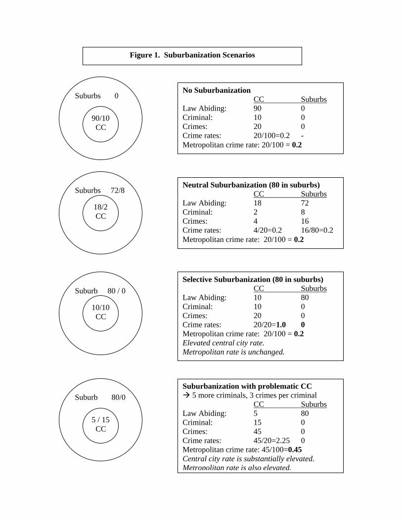
might influence crime by describing a series of hypothetical scenarios. Although simplistic, the

scenarios provide useful insights. They illustrate that suburbanization can lead to increased

central city crime rates whether or not the effect is causal, which presents a challenge for

empirical research.

In the first scenario, we assume there is no suburbanization: all 100 persons reside in the

central city. Ninety percent are law abiding, and 10 percent are criminals. Each criminal

commits two crimes per unit of time, so that 20 crimes occur. The crime rate (defined here

simply as crimes per person) is therefore 20/100 or 0.2. This situation is depicted in the top

panel of Figure 1. From this base, we examine three different possible patterns of

suburbanization. The first, shown in the middle panel of Figure 1, is neutral suburbanization,

- 7 -

which consists of a proportional redistribution of 80 percent of the population to the suburban

area. Criminals are just as likely to move to the suburbs as the law abiding, so that the both the

suburban area and the central city (CC) consist of 90 percent law-abiding persons and 10 percent

criminals. Assuming no change in the rate of offending, and assuming that most crimes are

committed locally, the suburban crime rate will equal the central city crime rate and the overall

metropolitan crime rate will not change. In this scenario, crime has merely been redistributed.

Clearly, this scenario is unlikely, because actual suburbanization tends to be selective with

respect to income, lifestyle, and preferences.

In the second suburbanization scenario, we model a highly selective movement from the

central city to the suburbs. Eighty law-abiding persons move to the suburbs, presumably in part

to escape the possibility of becoming a crime victim. Since all criminals remain in central city,

the crime rate in the suburbs is zero. The central city population now consists of ten law-abiding

persons and ten criminals. The central city crime rate quintuples to 1.0 because the reduced

population base divides the same number of crimes. This gives rise to the commonly observed

pattern of higher crime rates in the central city relative to the suburbs, but only because of the

change in the denominator of the central city crime rate. The overall metropolitan crime rate

remains unchanged, because in the metropolitan area as a whole there is the same population and

the same number of criminals committing the same number of crimes. The apparent rise in

crime is, in a sense, an illusion driven by the different suburbanization patterns of the criminal

and law-abiding segments of the population.

As discussed previously, many researchers going back to Shaw and Mckay (1942) have

argued that crime is not an exogenous phenomenon but is a function of the ecological

environment within which it occurs. In other words, criminal behavior, especially among

- 8 -

adolescents, is in part a response to social disorganization – neighborhoods with high levels of

stressful conditions such as poverty, family breakup, racial and ethnic discrimination, etc. If we

assume the criminals in our hypothetical models have disproportionate levels of economic and

social disadvantage, then the central-city neighborhoods in the selective suburbanization scenario

experience higher levels of poverty, family breakup, and other forms of disadvantage than

suburban neighborhoods. According to social disorganization theory, these extant social

conditions of the central city neighborhoods will have an independent effect of criminal

offending. Moreover, according to routine activity theory, the absence of capable guardians in

high-poverty neighborhoods will contribute to criminal offending, especially for property crime.

The bottom panel of Figure 1 describes a third suburbanization scenario, the problematic

central city, in which there are causal effects of neighborhood composition as alleged by Shaw

and McKay. First, there are three crimes per criminal because the harsh environment leads

people to commit more crimes, perhaps due to lax enforcement or reduced stigma. In addition,

the case assumes that the number of criminals also increases from 10 to 15 because of the

contagion effects of living in a very disadvantaged neighborhood. In other words, five people

who might have been law abiding under other circumstances capitulate to the environmental

influences of the central city neighborhood. For example, they may join a criminal gang to be

protected from other criminals. Clearly, the central city crime rate is higher in this scenario: it

rises to 2.25. Unlike the previous case however, the overall metropolitan crime rate is also

affected, rising from 0.2 to 0.45.

As in the selective suburbanization scenario, the problematic central city results in an

uneven pattern of crime rates. In the former case, however, the higher central city poverty rates

are the result of population movements that affect only the denominator of the crime rate

- 9 -

calculation. In the latter case, the higher central city crime rate results from changes in both the

numerator and the denominator of the crime rate. The changes in the numerator are casually

induced by post-sorting neighborhood conditions.

There are several important implications. First, an observed neighborhood-level

correlation between poverty (or some other measure of disadvantage) and crime is a necessary

but not sufficient condition to conclude that the former causes the latter. Both selective

suburbanization and the problematic central city scenarios result in such a correlation, but only in

the latter case is correlation causal. Even in that case, only part of the correlation results from

Shaw and Mckay-type effects, while the rest of the correlation is a reflection of sorting. It also

follows that an observed correlation between some measure of suburbanization and central city

poverty rates is not sufficient to conclude that suburbanization contributes to central city crime.

However, if problematic social conditions do exacerbate crime, metropolitan-level crime rates

will also be affected, because the total amount of crime is increased. The change in metropolitan

crime rates, unlike the change in central city crime rates, does potentially identify a causal effect.

These insights point to an empirical strategy. There is an expected level of crime in any

metropolitan area base on its population size, demographic composition, age structure, and

income level. If suburbanization affects the incidence of crime in a causal way, suburbanization

should predict crime at the metropolitan level after controlling for these baseline characteristics.

Further, to obtain unbiased estimates of the effect of suburbanization on crime net of baseline

characteristics, we must take into account the reciprocal relationship between suburbanization

and crime. If the spatial organization of the metropolitan area has causal effects on crime, these

effects could vary by the specific type of crime committed, so we distinguish violent crimes from

property crimes in our analysis.

- 10 -

Data and Variables

Crime Rates.

The crime rate is defined as the number of crimes per some unit of population, usually

100,000. Data on the number of crimes of different types are obtained from the Federal Bureau

of Investigation’s Uniform Crime Reports (UCR) program. Over 18,000 policing jurisdictions

across the United States provide UCR data. However, because UCR is “a voluntary program,”

the first-line police agencies do not submit mandatory reports, introducing another source of

error (Maltz & Targonski, 2002). Moreover, crime data is subject to errors based on inconsistent

enforcement and underreporting by victims.

UCR data is available in two different types: agency-level data and county-level data,

each with its own advantages. Police agencies have highly varied and sometimes overlapping

jurisdictions. Because we focus on metropolitan areas, which are composed of counties, we

aggregate county-level data to calculate the overall metropolitan area crime rate. Though the

study uses county-level crime data that is more appealing than agency-level data for our

purposes, the county-level data has some problems as well (Maltz & Targonski, 2002). Because

agencies’ jurisdictions sometimes overlap, and because the agencies may use incorrect or

inconsistent ways to estimate the population they serve, population figures in this data may not

be correct. We observed gross discrepancies between Census and UCR population figures. We

therefore use the population figures from Census data.

The county-level data set provides arrests for Part I offenses (murder, rape, robbery,

assault, burglary, larceny, auto theft, and arson) and for Part II offenses (forgery, fraud,

embezzlement, vandalism, weapons violations, sex offenses, drug and alcohol abuse violations,

gambling, vagrancy, curfew violations, and runaways). We focus on arrests for Part I offenses

- 11 -

(murder, rape, robbery, assault, burglary, larceny, auto theft, and arson). We subdivide these into

two categories: violent crime, including murder, rape, robbery, and assault; and property crime,

including burglary, larceny, auto theft, and arson.

Suburbanization Indicators

Several different measures of suburbanization are used to capture different dimensions of

the concept (Galster, et al., 2001; Yang & Jargowsky, 2006). The first suburbanization measure

is the density gradient. Although previous literature often focused on the relationship between

crime and population density in a given neighborhood or city, population density in a single

jurisdiction does not fully capture the meaning of suburbanization. If we define suburbanization

as “the enlargement and spread of a functionally integrated population over an increasingly wide

expanse of territory” (Berry & Kasarda, 1977), a measure is needed that captures the degree to

which a metropolitan area’s population is spread over a large area and that explicitly compares

density in the central city with density in the suburban areas. The density gradient gets at the

contrast between a centralized urban population and one that is more spread out. The density

gradient shows us how much the population density declines with increasing distance from the

central city. As an area becomes more suburbanized, the density gradient would increase

because the density gradient flattens out, i.e. the gradient becomes less negative. Given that we

hypothesize that suburbanization leads to higher crime levels, a positive coefficient is expected.

Although we prefer the density gradient, we also include the metropolitan area’s average

population density as a second measure of suburbanization. Though there are a variety of

concerns about usefulness of population density, it has frequently been used as a tool to estimate

whether a metropolitan area is compact or not. Some metropolitan areas including Los Angeles

have a high population density yet are also considered to have a high level of suburban sprawl.

- 12 -

Lower population density would be expected with a higher level of suburbanization, so we

expect a negative coefficient on density.

The third suburbanization measure is the percentage of the metropolitan area’s population

residing in the central city. Although frequently used in prior research, this measure may be

criticized on several grounds. It varies with region, era of metropolitan growth, land

configuration, and other factors. Since U.S. metropolitan areas tend to have significantly

different central city sizes relative to their total area, the percentage of central city population

might reflect factors other than suburbanization per se. With that caveat, a lower percentage of

central city population indicates metropolitan area is more suburbanized, so a negative

coefficient is expected.

The fourth measure of suburbanization is the average commuting time to work, which

reflects changing preferences for location and greater mobility of workers and firms. As

suburbanization increases, we expect longer travel time for metropolitan residents.

In summary, we have four measures of suburbanization: the density gradient, the average

population density, the percentage residing in the central city, and the average travel time to

work. If suburbanization increases crime net of other factors, we expect positive coefficients for

the density gradient and average travel time. We expect negative coefficients for average

population density and percentage in the central city, which vary inversely with suburbanization.

Factor analysis could be used to combine these four indicators into a single measure. However,

each of these factors represents a distinct aspect of suburbanization, rather than alternative

measures of a single underlying construct. Moreover, we believe that at least one of the

measures (percent of population in the central city) is inherently flawed. Given these

considerations, we have retained the individual indicators rather than combining them.

- 13 -

Demographic Controls and Instruments

Our analysis strategy is to test whether suburbanization predicts crime rates at the

metropolitan level. Suburbanization is likely to be correlated with population demographics,

which also contribute to crime. Therefore, our analysis includes demographic variables

measured at the metropolitan level, such as population size, age structure, race and ethnic

composition, and median household income, derived from the U.S. Census. The question

addressed is whether, holding these population composition variables constant, the arrangement

of the population into cities and suburbs affects the crime rate.

In view of the possibility of reverse causality, i.e. a causal effect of crime on

suburbanization, we employ instrumental variables estimation in our final set of models.

Plausible instrumental variables must affect suburbanization but not crime (net of the

demographic variables mentioned above). In our analysis, eight variables are used as

instruments for suburbanization. The first three are the number of governments, public transit

usage, and air pollution. When metropolitan areas are politically fragmented, the level of

suburbanization is likely to be higher since multiple suburban communities can develop in a

rapid and uncoordinated way and engage in exclusionary zoning. Public transportation might be

also associated with suburbanization since highly suburbanized areas are more automobile

dependent and tend to have poor public transportation system. The number of governments in

the metropolitan area and the percentage of metropolitan area residents using public

transportation are both derived from the Census. High levels of air pollution, often exacerbated

by congested streets in the downtown area, might drive people out of the central city area and

towards the suburban fringe. The Air Quality Index (AQI) index is provided by U.S.

Environmental Protection Agency (EPA).

- 14 -

Another set of five instruments reflect geographic characteristics of metropolitan areas.

These variables were obtained from Professor Stephen Malpezzi’s website, which provides

useful datasets about population, housing, and urban development by metropolitan area.5

Model Specification The unit of analysis is the metropolitan area. A metropolitan area generally consists of

one or more central counties including one or several central cities, along with surrounding

counties closely related to the central city by commuting patterns and other factors. In the 2000

Census, the Census Bureau defined stand-alone Metropolitan Statistical Areas (MSAs), such as

Indianapolis, and Primary Metropolitan Statistical Areas (PMSAs), such as the Dallas PMSA and

the Ft. Worth PMSA. PMSAs are part of larger units known as Consolidated Metropolitan

Statistical Areas (CMSAs). In this paper, we combine MSAs and PMSAs, and do not employ

CMSAs, which are extremely large relative to MSAs.

We model metropolitan area crime rates as follows:

1 2 3 4 5 6 7 8

9 10 11 12

13 18 65i i i i i i i

i i i i i

VC P B H A A A ING D C C T u

iα α α α α α α αα α α α

= + + + + + + +

+ + + + +

1 2 3 4 5 6 7 8

9 10 11 12

13 18 65i i i i i i i

i i i i i

PC P B H A A A ING D C C T v

iβ β β β β β β ββ β β β

= + + + + + + +

+ + + + +

The dependent variables, and represent violent and property crime rates of

metropolitan area i, respectively. Crime rates in metropolitan areas vary by demographic and

economic characteristics such as population, race, age, and income. P

iVC iPC

i is the log of population,

BBi is percentage Black, Hi is percentage Hispanic, A13i is the percentage of the MSA population

that is 13 to 17 years old, A18i is percentage 18 to 24 years old, A65i is percentage age over 65,

and INi is the median income. We observe the impact of suburbanization net of metropolitan

demographic factors by adding the four suburbanization indicators: Gi is the density gradient, Di

- 15 -

is the population density, CCi is the percentage of central city residents, and Ti is the mean travel

time to work. Finally, ui and vi are disturbance terms.

To address bias in the OLS regressions due to the endogeneity of suburbanization and

crime, we also employ instrumental variables regression (IV Regression), a general way to

obtain consistent estimators of the unknown coefficients when a regressor is correlated with the

error term (Stock & Watson, 2003). Theoretically, a valid instrumental variable has to satisfy

two conditions, know as instrument relevance and instrument exogeneity. First, an instrumental

variable should be correlated with the regressor, X. Second, an instrumental variable should be

uncorrelated with the error term. In the IV Models, the effect of our preferred suburbanization

measure, the density gradient, is estimated by instrumental variables:

1 2 3 4 5 6 7 8 913 18 65ii i i i i i iVC G P B H A A A INi iγ γ γ γ γ γ γ γ γ= + + + + + + + + + ε

i i

1 2 3 4 5 6 7 8 913 18 65ii i i i i i iPC G P B H A A A INδ δ δ δ δ δ δ δ δ= + + + + + + + + +η

where represents the density gradient instrumented with the variables described in the

previous section.

iG

Metropolitan areas vary widely in size; as a result, smaller metropolitan areas have larger

error variances than larger ones. Thus, all models are weighted by the square root of

metropolitan population (Maddala, 1977: 268-269). In addition to regression coefficients and

standard errors, standardized coefficients are presented to facilitate comparisons across variables

measured in different scales; they may be interpreted in terms of the effect in standard deviation

units of a one standard deviation change in the independent variables.

Findings Table 1 summarizes the variable descriptions and Table 2 displays descriptive statistics

for the variables. Crime rates vary significantly across metropolitan areas. For example, for

- 16 -

violent crime the minimum value of is 6.86 per 100,000 people while the maximum level is

1449.96 per 100,000 people. Population density tends to decrease with distance from central city,

so the density gradient is usually negative. As expected, except for Jersey City, NJ, all

metropolitan areas have a negative density gradient. Population densities, percentage of central

city population, and – to a lesser extent – mean travel time to work also vary a great deal from

one metropolitan area to another.

Table 3 shows the OLS regression results for metropolitan violent and property crime

rates. For violent crime, population size, black, and Hispanic are positive and statistically

significant, so large populations and high percentages of black and Hispanic residents are

associated with higher violent crime rates. Income is negative and significant, as expected.

However, some signs are not consistent with general expectations. For instance, “Age 13-17”

and “Age 18-24” are negatively significant, implying that a higher percentage of young

population leads to less violent crime. “Age 65 and more” is not statistically significant for

violent crime.

The estimated impact of suburbanization on crime differs depending on the measurement

of suburbanization. For violent crime, population density and the proportion of population in the

central city are significant. The negative coefficient of population density indicates that high

population density leads to a lower crime rate, consistent with the hypothesis that

suburbanization causes a higher crime rate. However, the sign of the coefficient for the

proportion of population in the central city is positive, contrary to expectations. As noted

previously, we question the efficacy of this measure and include it to demonstrate the importance

of the choice of the measure of suburbanization used. The density gradient and the mean travel

time are positive as expected, but not statistically significant. As a group, the suburbanization

- 17 -

measures are jointly significant (F=3.19, p<0.05). Taken together, these results are weakly

supportive of an impact of suburbanization on violent crime, particularly if one discounts for the

reversed sign on proportion in the central city. However, the endogeneity of suburbanization

may plague these results, which will be addressed below.

Table 3 also displays the results for the property crime rate as a dependent variable. Note

that there are many more property crimes than violent crimes, so the regression coefficients have

a different scale. For this reason, standardized coefficients are provided in the column labeled

“beta.” Several demographic and economic factors are statistically significant. Both percentage

black and Hispanic are significant and positive, so higher percentages of black and Hispanic

residents are associated with higher property crime. However, a few control variables have

different impacts on property crime than on violent crime. Income is negative but not significant.

Gross population is negatively related with property crime. The age structure variables are not

significant.

The impact of the various suburbanization measures also differs depending on the type of

crime. For property crime, both the density gradient and population density are significant and

consistent with suburbanization leading to more crime. The standardized coefficients show that

the effect is larger in magnitude for property crime than violent crime. The coefficient on central

city population, as in the case of violent crime, is inconsistent with the hypothesis. Travel time is

insignificant. A joint test of the suburbanization variables is significant (F=15.85, p<0.001).

The results from two-stage least squares model in Table 4 allow for the endogeneity of

suburbanization. The model includes our preferred measure of suburbanization (the density

gradient) as a regressor and crime (both violent crime and property crime) as dependent variables.

The model employs eight instruments for suburbanization: the number of governments, public

- 18 -

transit, air pollution, and five geographic characteristics of the metropolitan area. As shown in

Table 4, the coefficients of the instrumented density gradient in both the violent and property

models are positive and significant, further supporting the hypothesis that suburbanization leads

to higher crime rates.

Discussion Both demographic and geographic characteristics play a role in explaining high crime

rates in central cities or specific inner-ring suburban regions. Sociologists and criminologists

have long argued that truly disadvantaged neighborhoods in central cities are likely to lead to

higher crime rates. Even though many researchers have noted ecological effects of poor

neighborhoods on crime, generally these analyses have not separated the causal and

compositional effects of suburbanization on central city crime. We argue that Shaw and McKay-

type effects of neighborhood environment on crime can be identified by linking metropolitan

crime rates to measures of suburbanization. This method suffers from the relatively small

number of metropolitan areas and the high correlation and endogeneity of variables measured at

the metropolitan level, and therefore is relatively weak in the empirical sense. The benefit of this

empirical strategy is that it does not confuse true causal effects with changes in the central city

crime rate caused by the out-migration of the denominator.

The regressions in Tables 3 and 4 provide support for the hypothesis that suburbanization

increases crime rates in the central city over and above compositional effects. The increase in

crime is great enough to be measured at the metropolitan level. In particular, the relation

between suburbanization and crime seems to be stronger for property crime than violent crime.

The contrast between violent crime and property crime is consistent with empirical research on

routine activity theory (Stahura and Sloan 1988). The results, however, are sensitive to the

- 19 -

specific indicator used to measure suburbanization. The percentage of metropolitan population

residing in the central city, for example, indicates that suburbanization reduces crime in most

models. Why does it differ from other indicators in regression results? As Farley (1987) noted,

the percent of the population in the central city is related to regional and historical factors other

than suburbanization. For example, there are 31 metropolitan areas with more than 70 percent

of their residents residing in central cities, 12 of which are located in Texas. Yet most analysts

consider metropolitan areas in Texas to be highly suburbanized. Therefore, we are skeptical of

using the percentage of the population in the central city as an indicator of suburbanization, as

is common in prior literature.

Based on the remaining suburbanization measures, we conclude that suburbanization has

a positive impact on the overall crime rates in metropolitan areas. In particular, the effect is

more robust in the property crime models than in the violent crime models. As a result, the

evidence presented here supports an argument that there is a positive relationship between

suburbanization and metropolitan crime, operating via the effect on the economic and social

isolation of central city neighborhoods.

The models presented here must be considered preliminary, and are likely to suffer from

left out variable bias. Factors such as era of construction, topography, and idiosyncrasies of the

local housing market may affect both crime and suburbanization. In future research, we will

attempt to control these factors, at least to the extent that they were constant over time, by

estimating fixed effects models based on several decades of census and crime data. Whether or

not the findings presented here are confirmed by longitudinal analyses, this paper establishes an

important methodological point: past research has not clearly distinguished between the

compositional and causal effects of suburbanization on central city crime levels.

- 20 -

References

Alba, R. D., Logan, J. R., & Bellair, P. (1994). Living with Crime: The Implications of Racial/Ethnic Differences in Suburban Location. Social Forces, 73(2), 395-434.

Angel, S. (1968). Discouraging crime through city planning. (Paper No. 75). Berkeley, CA: Center for Planning and Development Research, University of California at Berkeley.

Barber, N. (2000). The Sex Ratio as a Predictor of Cross-National Variation in Violent Crime. Cross-Cultural Research, 34(3), 264-282.

Beasley, R. W., & Antunes, G. (1974). The etiology of urban crime: An ecological analysis. Criminology, 4, 439-461.

Berry, J. L., & Kasarda, J. D. (1977). Contemporary Urban Ecology. New York: Macmillan Publishing Co.

Booth, A., Welch, S., & Johnson, D. R. (1976). Crowding and urban crime rates. Urban affairs quarterly, 11, 291-307.

Bradford, D. F., & Kelejian, H. H. (1973). An Econometric Model of the Flight to the Suburbs. The Journal of Political Economy, 81(3), 566-589.

Burnham, R., Feinberg, R. M., & Husted, T. A. (2004). Central city crime and suburban economic growth. Applied Economics, 36, 917-922.

Bursik, R. J. (1988). Social Disorganization and Theories of Crime and Delinquency. Criminology, 26, 519-551.

Bursik, R. J. & Grasmick, H. G. (1993). Neighborhoods and Crime. San Francisco: Lexington Books.

Case, A. C. & Katz, L. F. (1991). The Company You Keep: The Effects of Family and Neighborhood on Disadvantaged Youths. (Working Paper No. 3705). Cambridge, MA: Natural Bureau of Economic Research.

Cohen, L. E. & Felson, M. (1979). Social change and crime rate trends: A routine activity approach, American Sociological Review, 44: 588-605.

Cullen, J. B. & Levitt, S. D. (1999). Crime, Urban Flight, and the Consequences for Cities. The Review of Economics and Statistics, 81(2), 159-169.

Farley, J. E. (1987). Suburbanization and Central-City Crime Rates: New Evidence and a Reinterpretation. The American Journal of Sociology, 93(3), 688-700.

Galle, O. R. (1973). Population density, social structure, and interpersonal violence: an intermetropolitan test of competing models. Paper presented at the annual meeting of the American Psychological Association, Montreal.

Galster, G., Hanson, R., Ratcliffe, M. R., Wolman, H., Coleman, S. & Freihage, J. (2001). Wrestling sprawl to the ground: Defining and measuring an elusive concept. Housing Policy Debate, 12, 681-717.

Gibbs, J. P., & Erickson, M. L. (1976). Crime Rates of American Cities in an Ecological Context. American Journal of Sociology, 82, 605-620.

Jacobs, J. (1961). The death and life of great American cities. New York: Random House.

Jargowsky, P. A. (1997). Poverty and place: ghettos, barrios, and the American city. New York: Russell Sage Foundation.

Jargowsky, P. A. (2002). Sprawl, Concentration of Poverty, and Urban Inequality. In G. Squires (Ed), Urban Sprawl: causes, consequences and policy response (pp.39-72). Washington, DC: The Urban Institute Press.

Jarrell, S., & Howsen, R. M. (1990). The Transient Crowing and Crime: The More ‘Strangers’ in an Area, the More Crime Except for Murder, Assault and Rape. American Journal of Economics and Sociology, 49(4), 483-494.

Joassart-Marcelli, Pascale M., Juliet A. Musso, and Jennifer R. Wolch. (2005). “Fiscal Consequences of Concentrated Poverty in a Metropolitan Region.” Annals of the Association of American Geographers 95: 336–356.

Jordan, S., Ross, J. P., & Usowski, K. G. (1998). U.S. suburbanization in the 1980s. Regional Science and Urban Economics, 28, 611-627.

Kling, J. R., Ludwig, J, & Katz, L. F. (2005). Neighborhood Effects on Crime for Female and Male Youth: Evidence From a Randomized Housing Voucher Experiment. The Quarterly Journal of Economics, 120(1), 87-130.

Kposowa, A. J., Breault, K. D., & Harrison, B. M. (1995). Reassessing the Structural Covariates of Violent and Property Crimes in the USA: a County Level Analysis. The British Journal of Sociology, 46(1), 79-105.

Krivo, L. J., & Peterson, R. D. (1996). Extremely Disadvantaged Neighborhoods and Urban Crime. Social Forces, 75(2), 619-648.

Kvalseth, T. O. (1977). A note on the effects of population density and unemployment on urban crime. Criminology, 15(1), 105-110.

Liska, A. E., & Bellair, P. E. (1995). Violent-crime Rates and Racial Composition: Convergence Over Time. American Journal of Sociology, 101, 578-610.

Liska, A. E., Logan, J. R., & Bellair, P. E. (1998). Race and Violent Crime in the Suburbs, American Sociological Review, 63, 27-38.

Logan, J. R. (1978). Growth, Politics and the Stratification of Places, American Journal of Sociology, 84, 404-416.

Lorenz, K. (1967). On aggression. London: Methuen and Co.

Ludwig, J., Duncan, G. J., & Hirschfield, P. (2001). Urban Poverty and Juvenile Crime: Evidence from a Randomized Housing-Mobility Experiment. The Quarterly Journal of Economics, 116(2), 655-679.

Maddala, G.S. (1977). Econometrics. New York: McGraw-Hill.

Maltz, M. D., & Targonski, J. (2002). A Note on The Use of County-level UCR data. Journal of Quantitative Criminology, 18(3), 297-318.

Mieszkowski, P., & Mills, E. S. (1993). The Causes of Metropolitan Suburbanization. The Journal of Economic Perspectives, 7(3), 135-147.

Mladenka, K. R., & Hill, K. Q. (1976). A reexamination of the etiology of urban crime, Criminology. 13, 491-506.

Oh, J. (2005). A Dynamic Approach to Population Change in Central Cities and Their Suburbs: 1980-1990. American Journal of Economics and Sociology, 64(2), 663-681.

O’Sullivan, A. (2003). Urban Economics (5th ed.). New York: McGraw-Hill.

Park, R. E., Burgess, E., & Mckenzie, R. D. (1925). The City. Chicago: University of Chicago Press.

Pew Center for Civic Journalism, Princeton Survey Research Associates. (n.d.). Straight Talk From Americans – 2000: National Survey Results Retrieved March 10, 2006, from http:www.pewcenter.org/doingcj/research/r_ST2000nat1.html

Pressman, I., & Carol, I. (1971). Crime as a diseconomy of scale. Review of Social Economy, 29, 227-236.

Roncek, Dennis W. (1981). “Dangerous Places: Crime and Residential Environment”, Social Forces, 60(1): 74-96.

Sampson, R. J. (1987). Urban Black Violence: The Effect of Male Joblessness and Family Disruption. American Journal of Sociology, 93, 348-382

Sampson, Robert J., & Groves, W. Byron. (1989). “Community Structure and Crime: Testing Social-Disorganization Theory”, The American Journal of Sociology, 94(4): 774-802.

Sampson, R. J., Morenoff, J. D., & Earls, F. (1999). Beyond Social Capital: Spatial Dynamics of Collective Efficacy for Children. American Sociological Review, 64, 633-660.

Sampson, R. J., Raudenbush, S., & Earls, F. (1997). Neighborhoods and violent Crime: A Multilevel Study of Collective Efficacy. Science, 277, 918-924.

Sampson, R. J., & Wilson, W. J. (1995). Toward a Theory of Race, Crime and Urban Inequality. In H. Barlow (Ed.), Crime and Public Policy: Putting Theory to Work (pp. 37-56). Boulder, CO: Westview Press.

Shaw, C. R., & McKay, H. D. (1942). Juvenile delinquency and urban areas. Chicago: University of Chicago Press.

Schichor, D., Decker, D. L., & O’Brien, R. M. (1980). The relationship of criminal victimization, police per capita and population density in twenty-six cities. Journal of Criminal Justice, 8, 309-316.

Shihadeh, E. S., & Ousey, G. C. (1996). Metropolitan Expansion and Black Social Dislocation: The Link between Suburbanization and Central-City Crime. Social Forces, 75(2), 649-666.

Skogan, W. G. (1977). The Changing Distribution of Big-City Crime: A Multi-City Time Series Analysis. Urban Affairs Quarterly, 13, 33-48.

South, S. J., & Messner, S. F. (2000). Crime and Demography: Multiple Linkages, Reciprocal Relations, Annual Review of Sociology, 26, 83-106.

Stafford, M. C., & Gibbs, J. (1980). Crime Rates in an Ecological Context: Extension of a Proposition. Social Science Quarterly, 61, 653-665.

Stahura, J. M., & Sloan, J. J. (1988). Urban Stratification of Places, Routine Activities and Suburban Crime Rates, Social Forces, 66(4), 1102-1118.

Stock, J. H., & Watson, M. W. (2003). Introduction to Econometrics. Boston: Pearson Education.

Van Den Berghe, P. L. (1974). Bringing breasts back in: Toward a biosocial theory of aggression. American sociological review, 39(6), 777-788.

Whethersby, G. B. (1970, October). Some determinants of crime: An econometric analysis of major and minor crimes around Boston. Paper presented at the Thirty-eight National Meeting of the Operations Research Society of America, Ann Arbor, MI.

Wilson, W. J. (1987). The Truly Disadvantaged: The Inner City, the Underclass, and Public Policy. Chicago: University of Chicago Press.

Wolfgang, M. E., & Ferracuti, F. (1967). Subculture of violence. London: Social Science Paperbacks.

Yang, R., & Jargowsky, P. A. (2006). Suburban development and economic segregation in the 1990s. Journal of Urban Affairs, 28, 253-273.

Suburbs 0

90/10 CC

No Suburbanization CC Suburbs Law Abiding: 90 0 Criminal: 10 0 Crimes: 20 0 Crime rates: 20/100=0.2 - Metropolitan crime rate: 20/100 = 0.2

Suburb 80 / 0

10/10 CC

Selective Suburbanization (80 in suburbs) CC Suburbs Law Abiding: 10 80 Criminal: 10 0 Crimes: 20 0 Crime rates: 20/20=1.0 0 Metropolitan crime rate: 20/100 = 0.2 Elevated central city rate. Metropolitan rate is unchanged.

Figure 1. Suburbanization Scenarios

Suburbs 72/8

18/2 CC

Neutral Suburbanization (80 in suburbs) CC Suburbs Law Abiding: 18 72 Criminal: 2 8 Crimes: 4 16 Crime rates: 4/20=0.2 16/80=0.2 Metropolitan crime rate: 20/100 = 0.2

Suburbanization with problematic CC 5 more criminals, 3 crimes per criminal

CC Suburbs Law Abiding: 5 80 Criminal: 15 0 Crimes: 45 0 Crime rates: 45/20=2.25 0 Metropolitan crime rate: 45/100=0.45 Central city rate is substantially elevated. Metropolitan rate is also elevated.

Suburb 80/0

5 / 15 CC

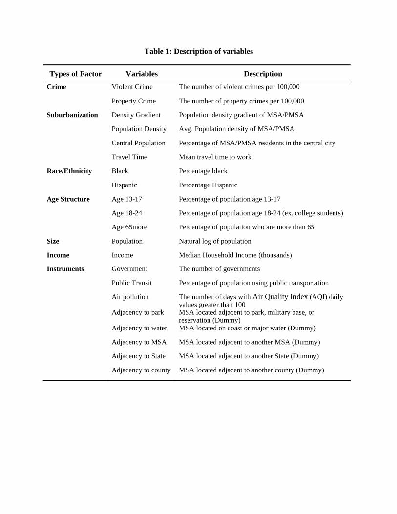
Table 1: Description of variables

Types of Factor Variables Description

Crime Violent Crime The number of violent crimes per 100,000

Property Crime The number of property crimes per 100,000

Suburbanization Density Gradient Population density gradient of MSA/PMSA

Population Density Avg. Population density of MSA/PMSA

Central Population Percentage of MSA/PMSA residents in the central city

Travel Time Mean travel time to work

Race/Ethnicity Black Percentage black

Hispanic Percentage Hispanic

Age Structure Age 13-17 Percentage of population age 13-17

Age 18-24 Percentage of population age 18-24 (ex. college students)

Age 65more Percentage of population who are more than 65

Size Population Natural log of population

Income Income Median Household Income (thousands)

Instruments Government The number of governments

Public Transit Percentage of population using public transportation

Air pollution The number of days with Air Quality Index (AQI) daily values greater than 100

Adjacency to park MSA located adjacent to park, military base, or reservation (Dummy)

Adjacency to water MSA located on coast or major water (Dummy)

Adjacency to MSA MSA located adjacent to another MSA (Dummy)

Adjacency to State MSA located adjacent to another State (Dummy)

Adjacency to county MSA located adjacent to another county (Dummy)

Table 2: Summary of Descriptive Statistics

N Mean Std. Dev Min Max

Violent Crime 323 434.91 237.10 6.86 1449.96

Property Crime 323 3718.29 1394.39 190.59 8104.93

Density Gradient 326 -0.19 0.11 -0.66 0.04

Population Density 323 441.16 957.50 5.41 13043.62

Central Population 323 0.42 0.20 0 1

Travel Time 323 22.58 3.78 15.06 38.93

Black 323 0.11 0.11 0.002 0.51

Hispanic 323 0.10 0.15 0.004 0.94

Age 13-17 323 0.07 .008 0.05 0.10

Age 18-24 332 0.05 0.01 0.02 0.18

Age 65+ 323 0.13 0.03 0.05 0.35

Population 323 12.79 1.05 10.97 16.07

Income 323 41.35 8.39 25.87 78.39

Government 331 35.67 44.72 1 319

Public Transit 323 0.02 0.04 0.001 0.47

Air Pollution 307 10.25 18.99 0 159

Adjacency to Park 306 0.23 0.42 0 1

Adjacency to Water 306 0.25 0.43 0 1

Adjacency to MSA 306 0.72 0.45 0 1

Adjacency to State 306 0.40 0.49 0 1

Adjacency to County 306 0.03 0.18 0 1

Table 3. OLS Regression Models for Metropolitan Crime Rates Violent Crime Property Crime b S.E. beta b S.E. beta Constant 134.38 272.75 -- 7906.60** 1811.97 -- Metropolitan Demographic Characteristics

Population (Log) 49.55** 12.76 0.26 -177.82* 84.75 -0.18

Income -7.63** 1.67 -0.29 -10.59** 11.11 -0.08

Black 1129.77** 123.32 0.46 4885.75** 819.24 0.38

Hispanic 657.07** 78.05 0.43 2581.38** 518.52 0.32 Age 13-17 -3899.74* 1765.29 -0.11 -20138.72* 11727.51 -0.11 Age 18-24 -3640.03** 1186.96 -0.17 6699.92** 7885.44 0.06

Age 65+ 343.79 455.68 0.04 -1843.92** 3027.26 -0.04

Suburbanization Indicators

Density Gradient 96.96 175.20 0.03 3530.61** 1163.92 0.20 Pop. Density -0.02** 0.008 -0.20 -0.31** 0.06 -0.46 Central Pop 199.58** 64.78 0.17 1472.51** 430.34 0.24 Travel Time 6.91 4.22 0.14 -22.42** 28.02 -0.09 F Test on all Suburbanization Indicators

F(4, 306) = 3.19 Prob > F = 0.0138

F(4, 306) = 15.85 Prob > F = 0.0000

R2 0.5835 0.3292 F 38.98** 13.65**

N 318 318 ** p ≤ .01; *p ≤ .05

Table 4. The Results from Two Stage Least Square (IV Regression Model)+

Violent Crime Property Crime b S.E. Beta b S.E. beta Population (Log) 5.79** 24.36 0.03 -1045.74** 193.08 -1.04

Income -4.21** 1.97 -0.16 -2.71** 15.58 -0.02

Black 1191.16** 133.92 0.49 4182.37** 1061.27 0.33

Hispanic 804.45** 84.34 0.54 2587.51** 668.41 0.33

Age 14-17 -7205.10** 2772.44 -0.17 -16035.67** 21971.27 -0.07

Age 18-24 543.53** 854.76 0.04 7159.82** 6773.84 0.11

Age 65+ 350.96** 640.97 0.05 -11144.47** 5079.57 -0.28 Density Gradient 1227.70** 620.62 0.34 19235.18** 4918.37 1.04

F 35.19** 7.42**

N 270 270

** p ≤ .01; *p ≤ .05 + The model employs eight instruments; the number of governments, public transit, air pollution, adjacency to a park, adjacency to water, adjacency to another metropolitan area, adjacency to a state boundary, and adjacency to a county boundary.

1 Calculated from FBI, Uniform Crime Reports, Table 12: Crime Trends by Population Group, 2004-2005. The crime rate is the number of crimes per 100,000 inhabitants. Suburban areas include law enforcement agencies in cities with less than 50,000 inhabitants and county law enforcement agencies that are within Metropolitan Statistical Areas. Suburban areas exclude all metropolitan agencies associated with a central city. 2In contrast, Jordan, Ross, and Usowski (1998) found that central city crime reduced suburbanization, the opposite of their expectation. 3 See also Kling, Ludwig, and Katz (2005). 4 While it is true that a positive relationship was more common (Lornez, 1967; van den Berghe, 1974; Wolfgang & Ferracuti, 1967; Booth & Johnson, 1976; Galle, 1973; Beasley & Antunes, 1974; Mladenka & Hill, 1976), several studies found a negative relationship (Jacobs, 1961; Angel, 1968; Weathersby, 1970; Pressman & Carol, 1971; Kvalseth, 1977; Schichor, Decker, & O’Brien, 1980). See also Jarrel and Howsen (1990), Kpososwa, Breault, and Harrison (1995), and Barber (2000). 5 Malpezzi’s website address for geographic data is www.bus.wisc.edu/realestate/doc/doc/smallmsa.xls.