Embed Size (px)
Citation preview
Stats 95t-Tests
• Single Sample
• Paired Samples
• Independent Samples
William Sealy Gosset
t Distributions
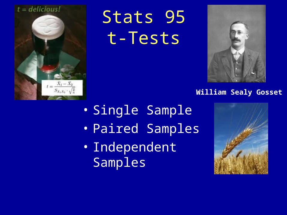
• t dist. are used when we know the mean of the population but not the SD of the population from which our sample is drawn
• t dist. are useful when we have small samples.
• t dist is flatter and has fatter tails
• As sample size approaches 30, t looks like z (normal) dist.
• Same Three Assumptions• Dependent Variable is scale
• Random selection
• Normal Distribution

Fat Tails Lose Weight With Larger Sample Size
The Robust Nature of the t Statistics
Unfortunately, we very seldom know the if the population is normal because usually all the information we have about a population is in our study, a sample of 10-20.
Fortunately,
1) distributions in social sciences often approximate a normal curve, and
2) according to Central Limit Theorem the sample mean you have gathered is part of a normal distribution of sample means, and
3) in practice t tests statisticians have found the test is accurate even with populations far from normal
The Robust Nature of the t Statistics
• The only situation in which using a t test is likely to give a seriously distorted result is when you are using a one-tailed test and the population is highly skewed.
When To Use Single Sample t-Statistic
• 1 Nominal Independent Variable
• 1 Scale Dependent Variable
• Population Mean, No Population Standard Deviation
Check Assumptions
• Random Selection
• Normal Shape Distribution
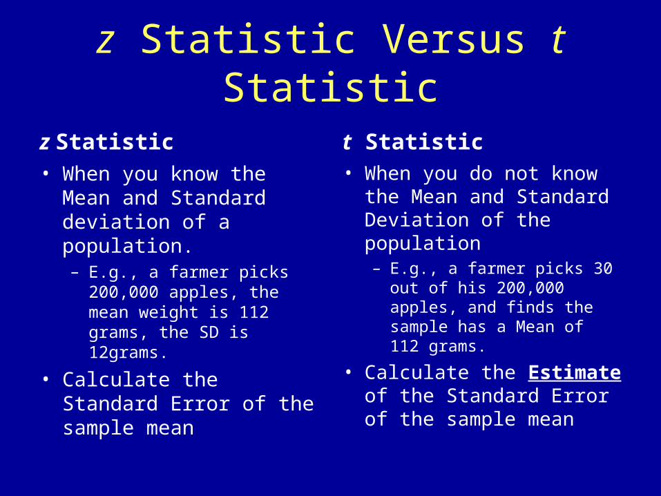
z Statistic Versus t Statistic
z Statistic
• When you know the Mean and Standard deviation of a population.– E.g., a farmer picks 200,000
apples, the mean weight is 112 grams, the SD is 12grams.
• Calculate the Standard Error of the sample mean
t Statistic
• When you do not know the Mean and Standard Deviation of the population– E.g., a farmer picks 30 out of
his 200,000 apples, and finds the sample has a Mean of 112 grams.
• Calculate the Estimate of the Standard Error of the sample mean
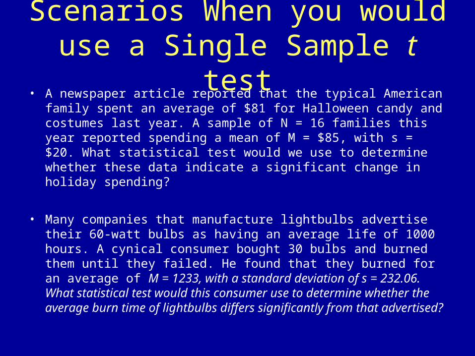
Scenarios When you would use a Single Sample t test
• A newspaper article reported that the typical American family spent an average of $81 for Halloween candy and costumes last year. A sample of N = 16 families this year reported spending a mean of M = $85, with s = $20. What statistical test would we use to determine whether these data indicate a significant change in holiday spending?
• Many companies that manufacture lightbulbs advertise their 60-watt bulbs as having an average life of 1000 hours. A cynical consumer bought 30 bulbs and burned them until they failed. He found that they burned for an average of M = 1233, with a standard deviation of s = 232.06. What statistical test would this consumer use to determine whether the average burn time of lightbulbs differs significantly from that advertised?
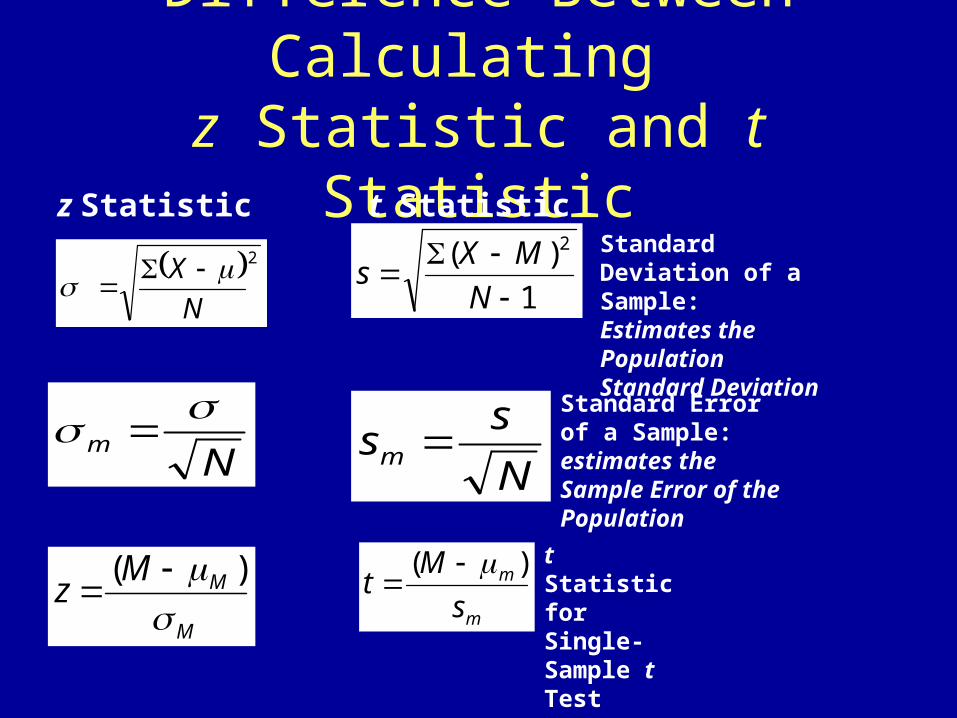
Difference Between Calculating z Statistic and t Statistic
z Statistic t Statistic
2
N
X
Nm
M
MMz
)(
N
ssm
Standard Error of a Sample: estimates the Sample Error of the Population
m
m
s
Mt
)(
t Statistic for Single-Sample t Test
1
)( 2
N
MXs
Standard Deviation of a Sample: Estimates the Population Standard Deviation
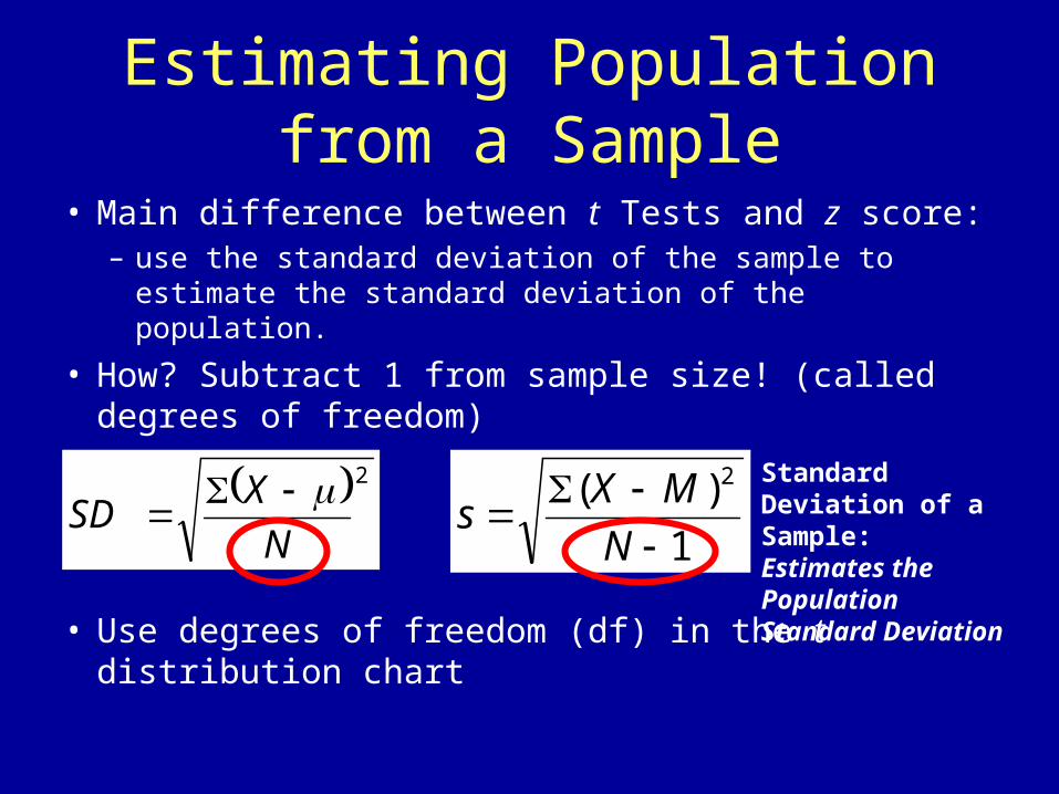
Estimating Population from a Sample
• Main difference between t Tests and z score: – use the standard deviation of the sample to estimate the
standard deviation of the population.
• How? Subtract 1 from sample size! (called degrees of freedom)
• Use degrees of freedom (df) in the t distribution chart
2
N
XSD
1
)( 2
N
MXs
Standard Deviation of a Sample: Estimates the Population Standard Deviation
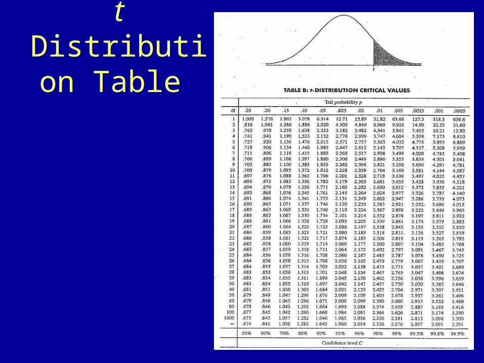
t Distribution Table
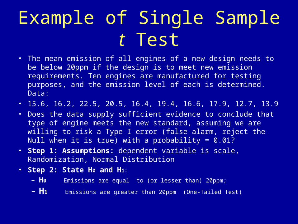
Example of Single Sample t Test
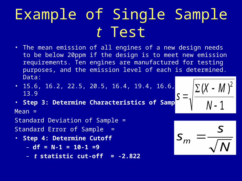
• The mean emission of all engines of a new design needs to be below 20ppm if the design is to meet new emission requirements. Ten engines are manufactured for testing purposes, and the emission level of each is determined. Data:
• 15.6, 16.2, 22.5, 20.5, 16.4, 19.4, 16.6, 17.9, 12.7, 13.9
• Does the data supply sufficient evidence to conclude that type of engine meets the new standard, assuming we are willing to risk a Type I error (false alarm, reject the Null when it is true) with a probability = 0.01?
• Step 1: Assumptions: dependent variable is scale, Randomization, Normal Distribution
• Step 2: State H0 and H1: – H0 Emissions are equal to (or lesser than) 20ppm;
– H1 Emissions are greater than 20ppm (One-Tailed Test)
Example of Single Sample t Test
• The mean emission of all engines of a new design needs to be below 20ppm if the design is to meet new emission requirements. Ten engines are manufactured for testing purposes, and the emission level of each is determined. Data:
• 15.6, 16.2, 22.5, 20.5, 16.4, 19.4, 16.6, 17.9, 12.7, 13.9
• Step 3: Determine Characteristics of Sample
Mean =
Standard Deviation of Sample =
Standard Error of Sample =
• Step 4: Determine Cutoff
– df = N-1 = 10-1 =9
– t statistic cut-off = -2.822 N
ssm
1
)( 2
N
MXs
Example of Single Sample t Test
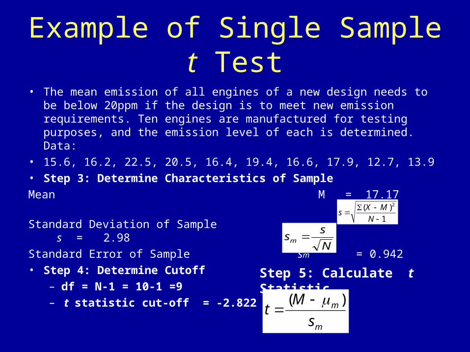
• The mean emission of all engines of a new design needs to be below 20ppm if the design is to meet new emission requirements. Ten engines are manufactured for testing purposes, and the emission level of each is determined. Data:
• 15.6, 16.2, 22.5, 20.5, 16.4, 19.4, 16.6, 17.9, 12.7, 13.9
• Step 3: Determine Characteristics of Sample
Mean M = 17.17
Standard Deviation of Sample s = 2.98
Standard Error of Sample sm = 0.942
• Step 4: Determine Cutoff
– df = N-1 = 10-1 =9
– t statistic cut-off = -2.822
Step 5: Calculate t Statistic
m
m
s
Mt
)(
N
ssm
1
)( 2
N
MXs
Example of Single Sample t Test
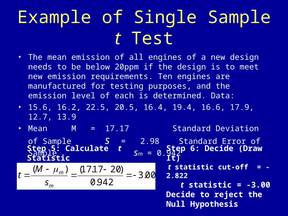
• The mean emission of all engines of a new design needs to be below 20ppm if the design is to meet new emission requirements. Ten engines are manufactured for testing purposes, and the emission level of each is determined. Data:
• 15.6, 16.2, 22.5, 20.5, 16.4, 19.4, 16.6, 17.9, 12.7, 13.9
• Mean M = 17.17 Standard Deviation of Sample s = 2.98
Standard Error of Sample sm = 0.942
Step 5: Calculate t Statistic
00.3942.0
)2017.17()(
m
m
s
Mt
Step 6: Decide (Draw It) t statistic cut-off = -2.822 t statistic = -3.00Decide to reject the Null Hypothesis

How to Write Results
• t(7) = -.79, p < .265, d = -.29
• t Indicates that we are using a t-Test
• (9) Indicates the degrees of freedom associated with this t-Test
• -.79 Indicates the obtained t statistic value
• p < .265 Indicates the probability of obtaining the given t value by chance alone
• d = -.29 Indicates the effect size for the significant effect (the magnitude of the effect is measured in standard deviation units)
Paired Sample t Test
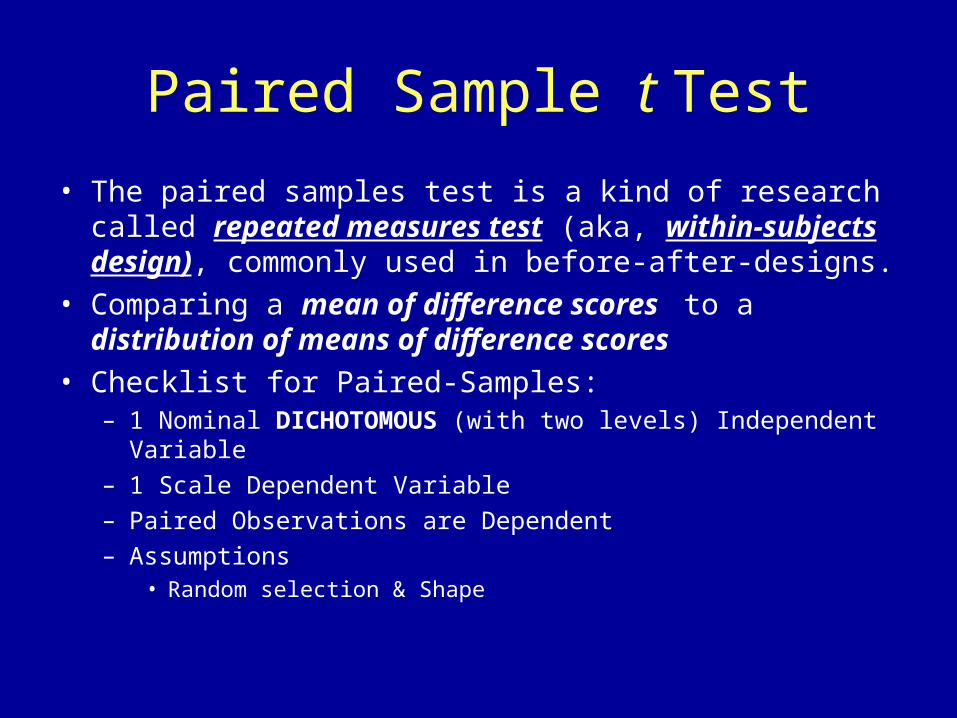
• The paired samples test is a kind of research called repeated measures test (aka, within-subjects design), commonly used in before-after-designs.
• Comparing a mean of difference scores to a distribution of means of difference scores
• Checklist for Paired-Samples:– 1 Nominal DICHOTOMOUS (with two levels) Independent Variable
– 1 Scale Dependent Variable
– Paired Observations are Dependent
– Assumptions• Random selection & Shape
Paired-Samples t-Test
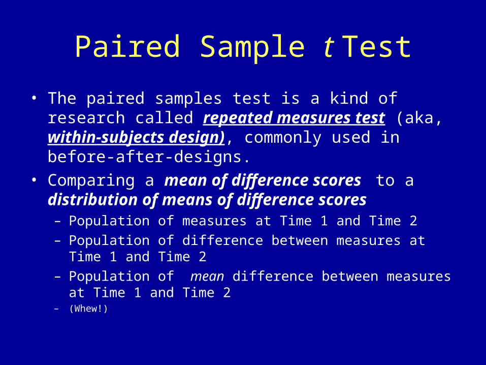
Paired Sample t Test
• The paired samples test is a kind of research called repeated measures test (aka, within-subjects design), commonly used in before-after-designs.
• Comparing a mean of difference scores to a distribution of means of difference scores– Population of measures at Time 1 and Time 2
– Population of difference between measures at Time 1 and Time 2
– Population of mean difference between measures at Time 1 and Time 2– (Whew!)
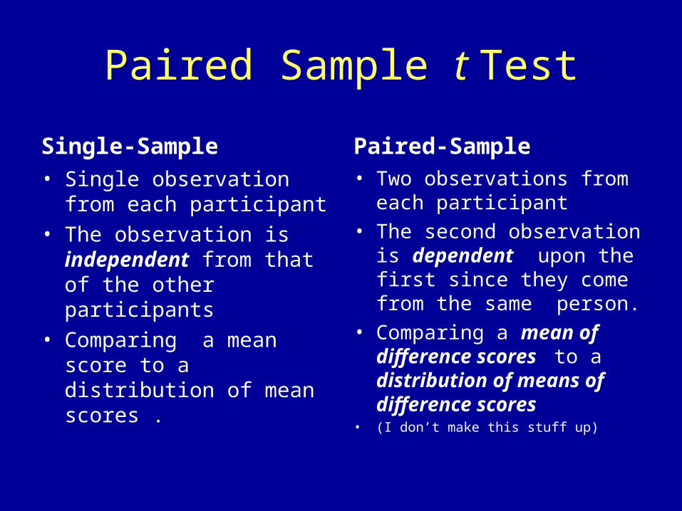
Paired Sample t Test
Single-Sample
• Single observation from each participant
• The observation is independent from that of the other participants
• Comparing a mean score to a distribution of mean scores .
Paired-Sample
• Two observations from each participant
• The second observation is dependent upon the first since they come from the same person.
• Comparing a mean of difference scores to a distribution of means of difference scores
• (I don’t make this stuff up)
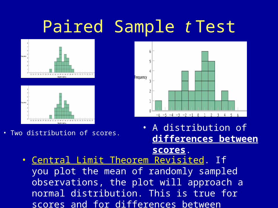
Paired Sample t Test
• Two distribution of scores. • A distribution of
differences between scores.
• Central Limit Theorem Revisited. If you plot the mean of randomly sampled observations, the plot will approach a normal distribution. This is true for scores and for differences between matched scores.
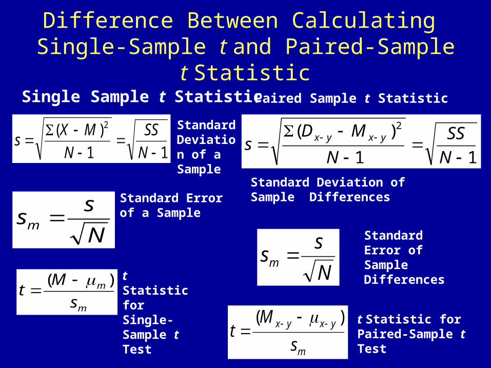
Difference Between Calculating Single-Sample t and Paired-Sample t Statistic
Single Sample t Statistic
N
ssm
Standard Error of a Sample
m
m
s
Mt
)(
t Statistic for Single-Sample t Test
11
)( 2
N
SS
N
MXs
Standard Deviation of a Sample
Paired Sample t Statistic
m
yxyx
s
Mt
)(
t Statistic for Paired-Sample t Test
11
)( 2
N
SS
N
MDs yxyx
N
ssm
Standard Error of Sample Differences
Standard Deviation of Sample Differences
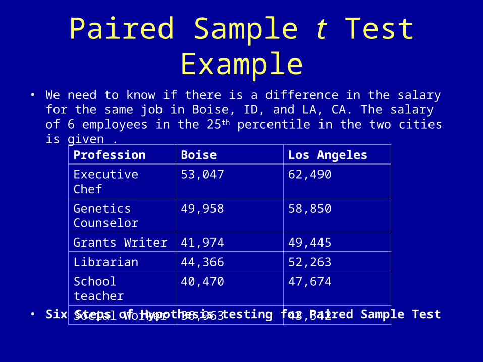
Paired Sample t Test Example
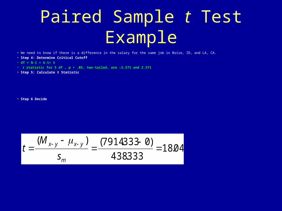
• We need to know if there is a difference in the salary for the same job in Boise, ID, and LA, CA. The salary of 6 employees in the 25th percentile in the two cities is given .
• Six Steps of Hypothesis testing for Paired Sample Test
Profession Boise Los Angeles
Executive Chef 53,047 62,490
Genetics Counselor 49,958 58,850
Grants Writer 41,974 49,445
Librarian 44,366 52,263
School teacher 40,470 47,674
Social Worker 36,963 43,542
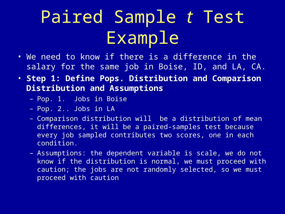
Paired Sample t Test Example
• We need to know if there is a difference in the salary for the same job in Boise, ID, and LA, CA.
• Step 1: Define Pops. Distribution and Comparison Distribution and Assumptions– Pop. 1. Jobs in Boise
– Pop. 2.. Jobs in LA
– Comparison distribution will be a distribution of mean differences, it will be a paired-samples test because every job sampled contributes two scores, one in each condition.
– Assumptions: the dependent variable is scale, we do not know if the distribution is normal, we must proceed with caution; the jobs are not randomly selected, so we must proceed with caution
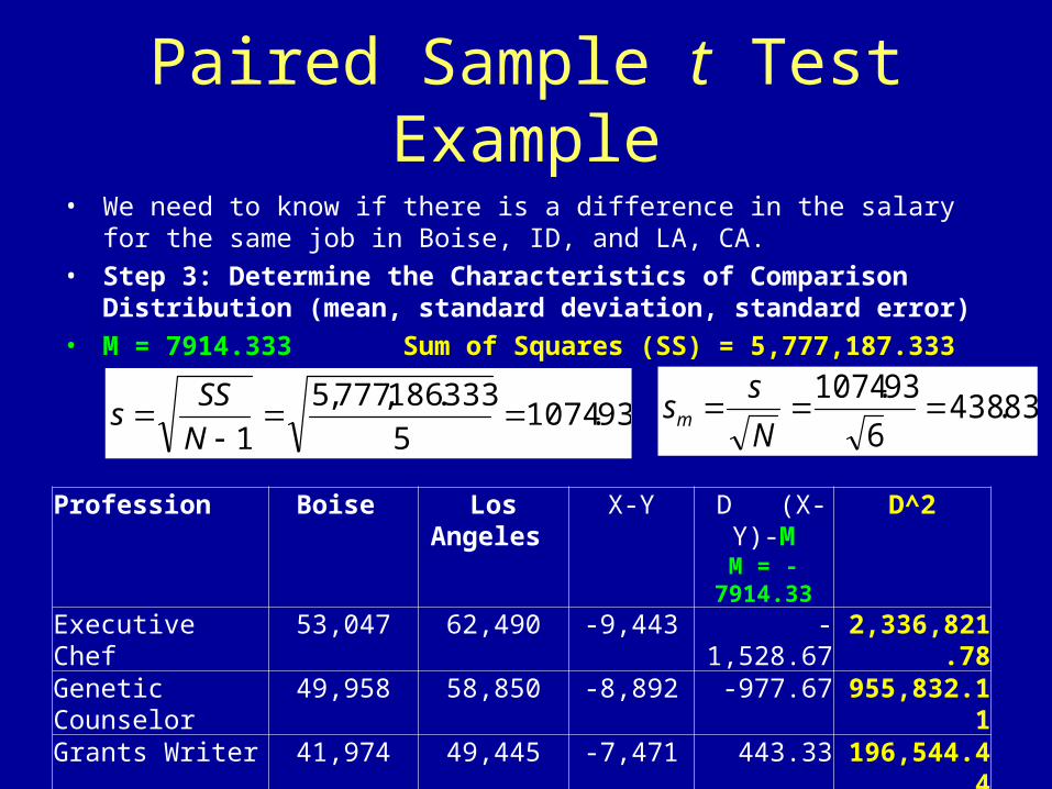
Paired Sample t Test Example
• We need to know if there is a difference in the salary for the same job in Boise, ID, and LA, CA.
• Step 3: Determine the Characteristics of Comparison Distribution (mean, standard deviation, standard error)
• M = 7914.333 Sum of Squares (SS) = 5,777,187.333
Profession Boise Los Angeles X-Y D (X-Y)-MM = -7914.33
D^2
Executive Chef 53,047 62,490 -9,443 -1,528.67 2,336,821.78
Genetic Counselor 49,958 58,850 -8,892 -977.67 955,832.11Grants Writer 41,974 49,445 -7,471 443.33 196,544.44Librarian 44,366 52,263 -7,897 17.33 300.44School teacher 40,470 47,674 -7,204 710.33 504,573.44Social Worker 36,963 43,542 -6,579 1,335.33 1,783,115.11
93.10745
333.186,777,5
1
N
SSs 83.438
6
93.1074
N
ssm
Paired Sample t Test Example• We need to know if there is a difference in the salary for the same job in Boise, ID, and LA, CA.
• Step 4: Determine Critical Cutoff
• df = N-1 = 6-1= 5
• t statistic for 5 df , p < .05, two-tailed, are -2.571 and 2.571
• Step 5: Calculate t Statistic
• Step 6 Decide
04.18333.438
)0333.7914()(
m
yxyx
s
Mt
How to Write Results
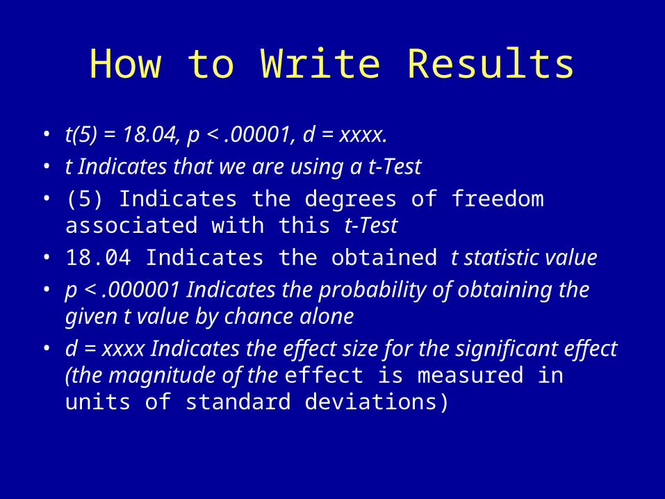
• t(5) = 18.04, p < .00001, d = xxxx.
• t Indicates that we are using a t-Test
• (5) Indicates the degrees of freedom associated with this t-Test
• 18.04 Indicates the obtained t statistic value
• p < .000001 Indicates the probability of obtaining the given t value by chance alone
• d = xxxx Indicates the effect size for the significant effect (the magnitude of the effect is measured in units of standard deviations)
Independent t-Test
Independent t Test
• Compares the difference between two means of two independent groups.
• You are comparing a difference between means to a distribution of differences between means.– Sample means from Group 1 and Group 2 compared to
a Population of differences between means of Group 1 and Group 2
Independent t Test
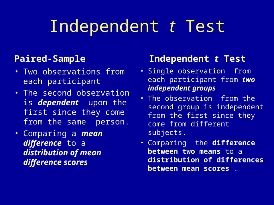
Independent t Test
• Single observation from each participant from two independent groups
• The observation from the second group is independent from the first since they come from different subjects.
• Comparing the difference between two means to a distribution of differences between mean scores .
Paired-Sample
• Two observations from each participant
• The second observation is dependent upon the first since they come from the same person.
• Comparing a mean difference to a distribution of mean difference scores

1
)( 22
N
MYs y
yxtotal dfdfdf
y
total
yx
total
xpooled s
df
dfs
df
dfs 222
1
)( 22
N
MXsx
x
pooledMx N
ss
22
y
pooledMy N
ss
22
222MyMxDifference sss
Independent t Test: Steps
Step 1
Step 2
Step 4
Step 3
Step 5
Calculate the corrected variance for each sample
Calculate the degrees of freedom
Calculate the pooled variance
Calculate the squared estimate of the standard error for each sample
Calculate estimated variance of the dist. of mean differences
Like the Standard error in a z test
In a z test you find SD, for ind. t, you take weighted avg of SD2
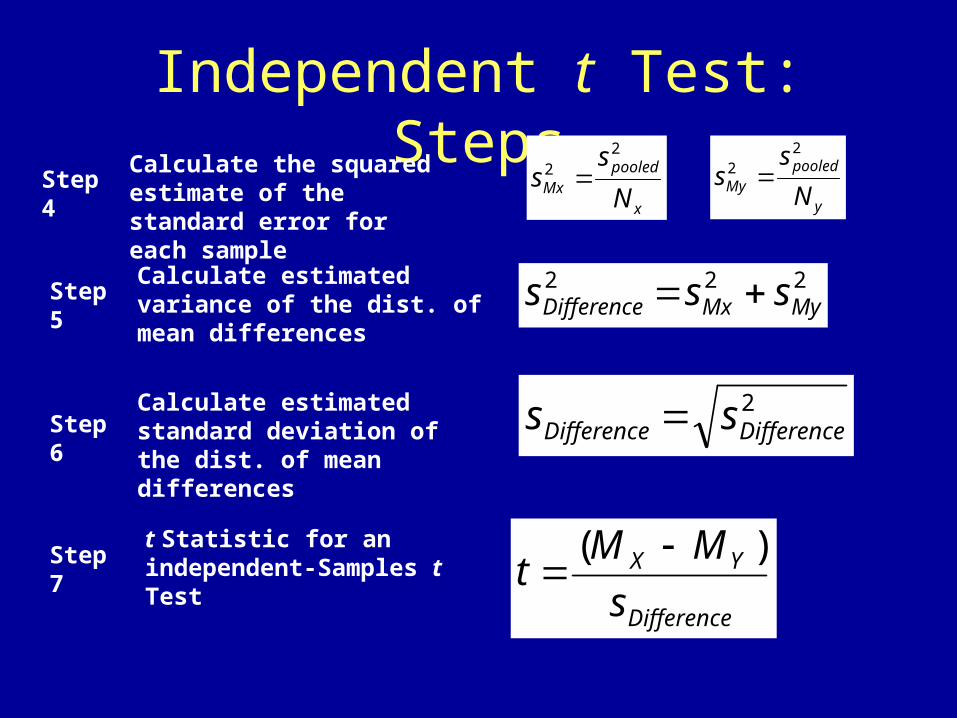
2DifferenceDifference ss
Independent t Test: Steps
Step 6
x
pooledMx N
ss
22
y
pooledMy N
ss
22
222MyMxDifference sss
Step 4
Step 5
Calculate the squared estimate of the standard error for each sample
Calculate estimated variance of the dist. of mean differences
Calculate estimated standard deviation of the dist. of mean differences
Difference
YX
s
MMt
)(
t Statistic for an independent-Samples t TestStep 7
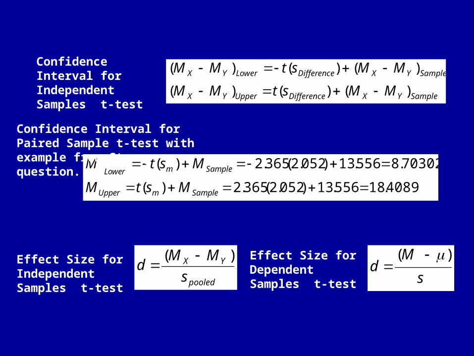
SampleYXDifferenceUpperYX
SampleYXDifferenceLowerYX
MMstMM
MMstMM
)()()(
)()()(
pooled
YX
s
MMd
)(
4089.18556.13)052.2(365.2)(
70302.8556.13)052.2(365.2)(
SamplemUpper
SamplemLower
MstM
MstM
Confidence Interval for Independent Samples t-test
Effect Size for Independent Samples t-test
Confidence Interval for Paired Sample t-test with example from Stroop question.
s
Md
)(
Effect Size for Dependent Samples t-test
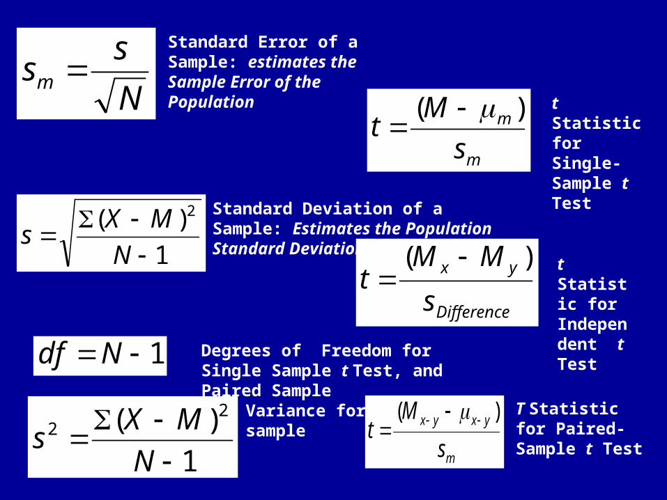
1
)( 22
N
MXs
Variance for a sample
1Ndf Degrees of Freedom for Single Sample t Test, and Paired Sample
N
ssm
Standard Error of a Sample: estimates the Sample Error of the Population
m
m
s
Mt
)(
t Statistic for Single-Sample t Test
1
)( 2
N
MXs
Standard Deviation of a Sample: Estimates the Population Standard Deviation
Difference
yx
s
MMt
)(
t Statistic for Independent t Test
m
yxyx
s
Mt
)(
T Statistic for Paired-Sample t Test
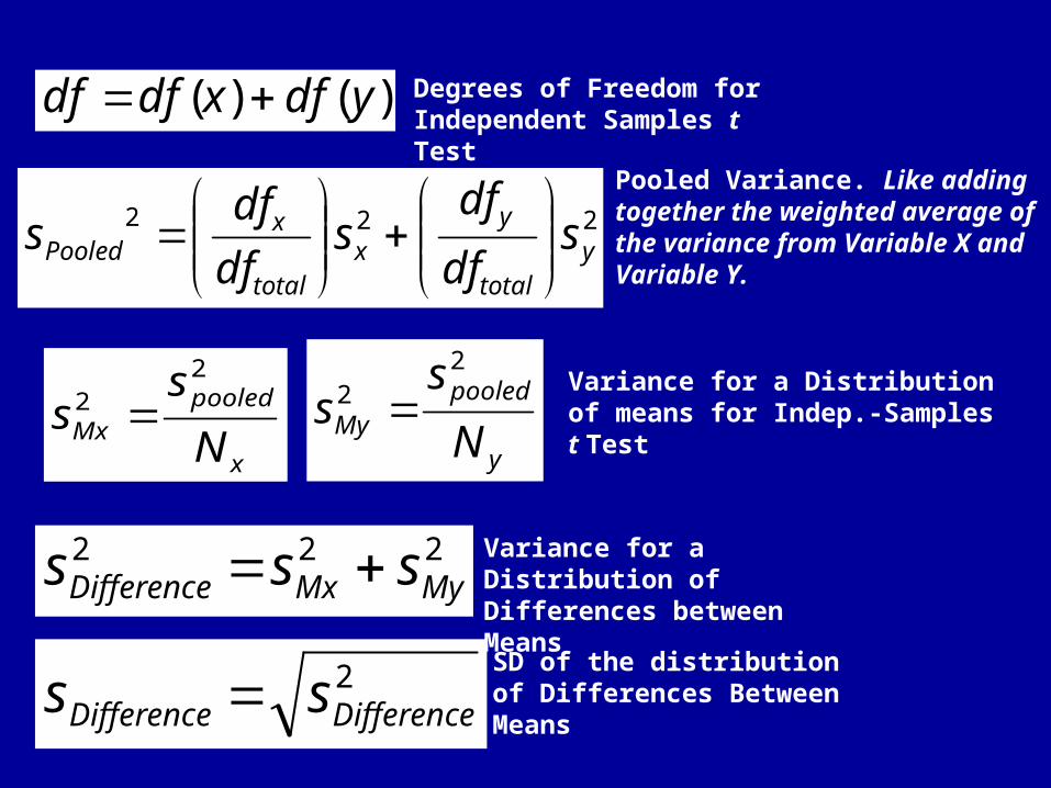
)()( ydfxdfdf Degrees of Freedom for Independent Samples t Test
222y
total
yx
total
xPooled s
df
dfs
df
dfs
Pooled Variance. Like adding together the weighted average of the variance from Variable X and Variable Y.
x
pooledMx N
ss
22
Variance for a Distribution of means for Indep.-Samples t Test
y
pooledMy N
ss
22
222MyMxDifference sss Variance for a Distribution of
Differences between Means
2DifferenceDifference ss
SD of the distribution of Differences Between Means
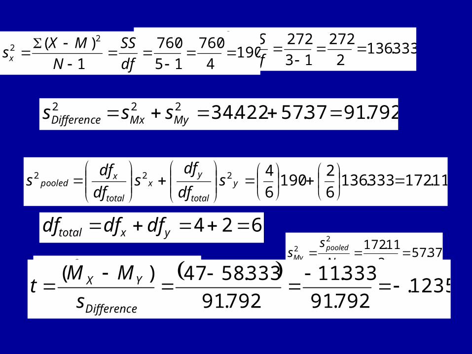
333.1362
272
13
272
1
)( 22
df
SS
N
MYs y 190
4
760
15
760
1
)( 22
df
SS
N
MXsx
624 yxtotal dfdfdf
11.172333.1366
2190
6
4222
y
total
yx
total
xpooled s
df
dfs
df
dfs
422.345
11.1722
2 x
pooledMx N
ss
37.573
11.1722
2 y
pooledMy N
ss
792.9137.57422.34222 MyMxDifference sss
1235.
792.91
333.11
792.91
333.5847)(
Difference
YX
s
MMt
16
09.61
11
)( 22
N
SS
N
Ms yxyx
11
)( 2
N
SS
N
Ms yxyx
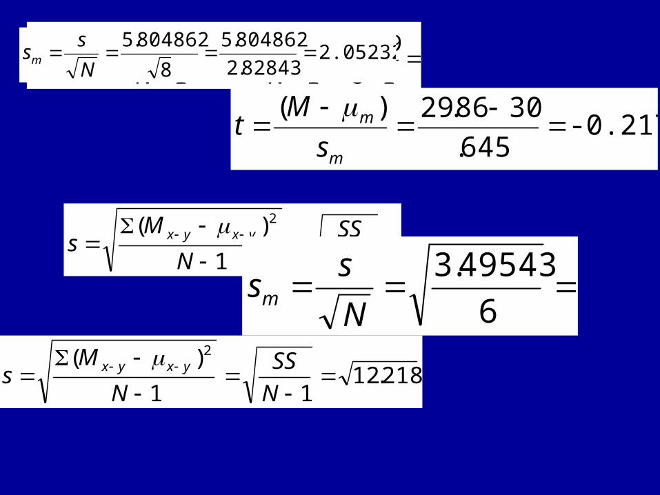
218.1211
)( 2
N
SS
N
Ms yxyx
6
49543.3
N
ssm
-0.2171645.
3086.29)(
m
m
s
Mt
2.05232982843.2
804862.5
8
804862.5
N
ssm
3.1362
667.272
11
)( 22
N
SSy
N
MYs y
yxtotal dfdfdf
1.1723.1366
2190
6
4222
y
total
yx
total
xpooled s
df
dfs
df
dfs
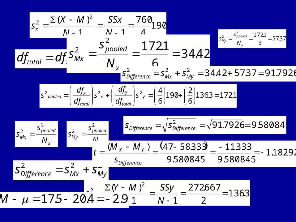
1904
760
11
)( 22
N
SSx
N
MXsx
x
pooledMx N
ss
22
y
pooledMy N
ss
22
222MyMxDifference sss
580845.97926.912 DifferenceDifference ss
42.346
1.1722
2 x
pooledMx N
ss
37.573
1.1722
2 y
pooledMy N
ss
7926.9137.5742.34222 MyMxDifference sss
18292.1
580845.9
333.11
580845.9
333.5847)(
Difference
YX
s
MMt
9.24.205.17 M
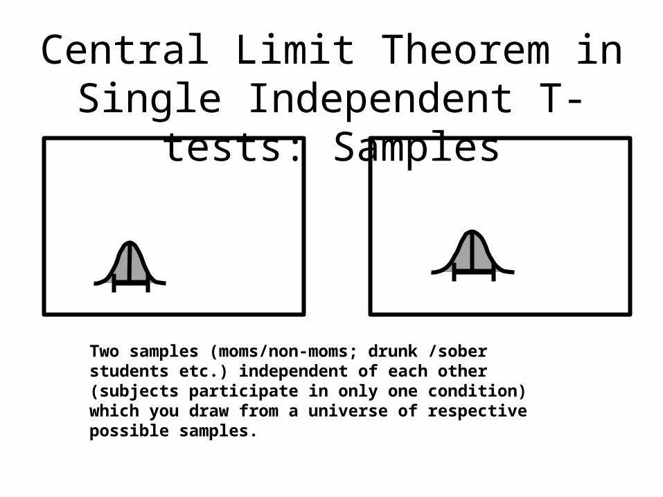
Central Limit Theorem in Single Independent T-tests: Samples
Two samples (moms/non-moms; drunk /sober students etc.) independent of each other (subjects participate in only one condition) which you draw from a universe of respective possible samples.
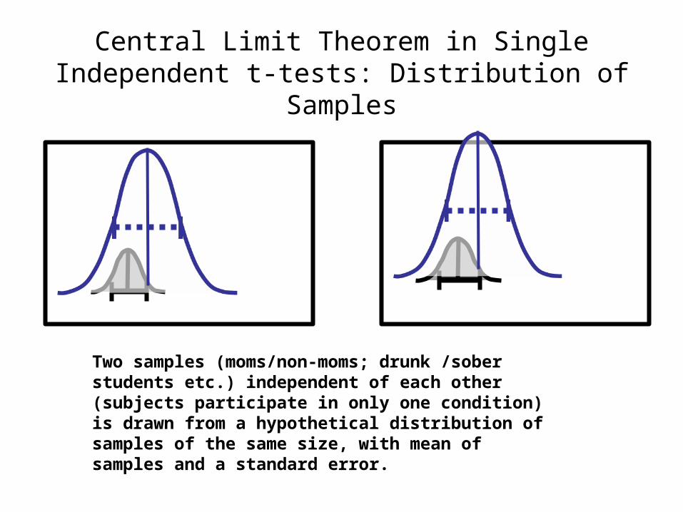
Central Limit Theorem in Single Independent t-tests: Distribution of Samples
Two samples (moms/non-moms; drunk /sober students etc.) independent of each other (subjects participate in only one condition) is drawn from a hypothetical distribution of samples of the same size, with mean of samples and a standard error.
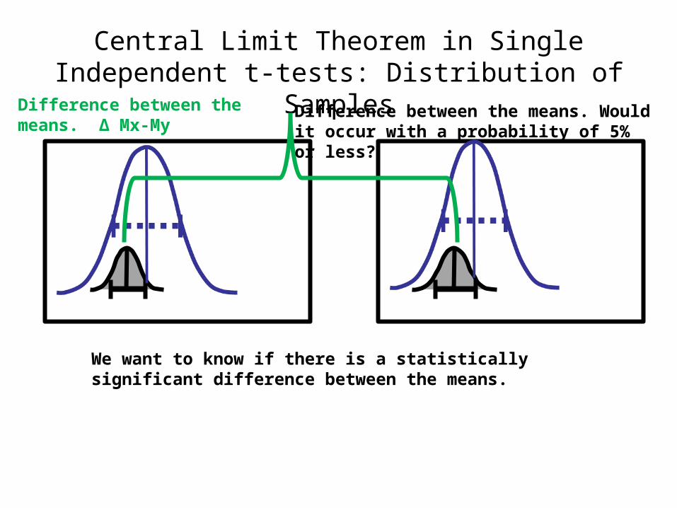
Central Limit Theorem in Single Independent t-tests: Distribution of Samples
We want to know if there is a statistically significant difference between the means.
Difference between the means. Would it occur with a probability of 5% or less?
Difference between the means. Δ Mx-My
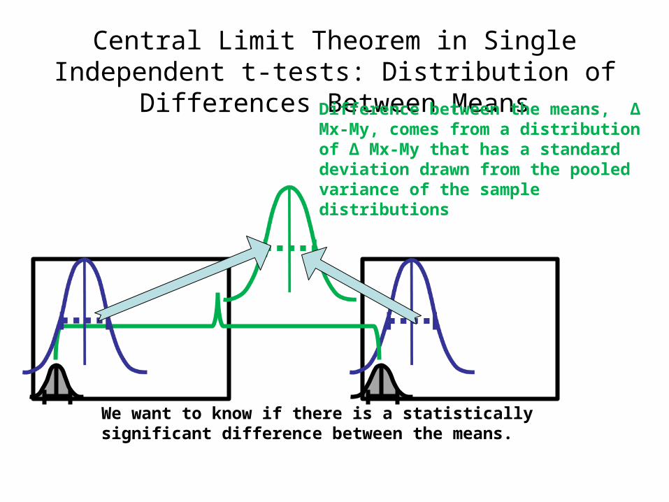
Central Limit Theorem in Single Independent t-tests: Distribution of Differences Between Means
We want to know if there is a statistically significant difference between the means.
Difference between the means, Δ Mx-My, comes from a distribution of Δ Mx-My that has a standard deviation drawn from the pooled variance of the sample distributions
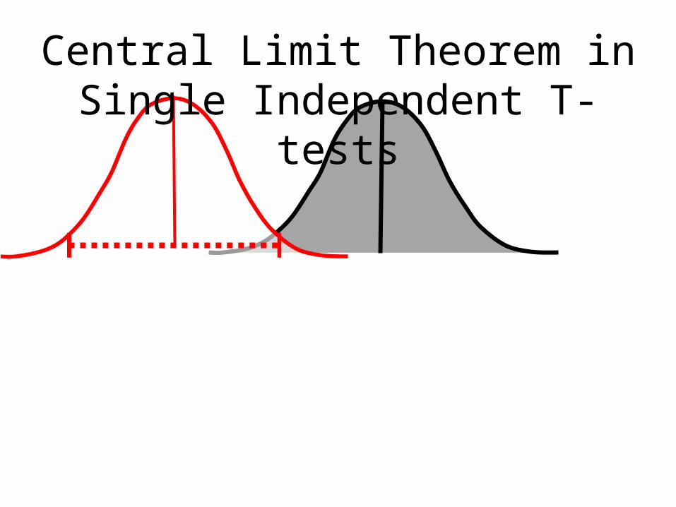
Central Limit Theorem in Single Independent T-tests