WILLIAM SEALY GOSSET: A HISTORY OFBEER AND STATISTICS

Presented to the Faculty of Mathematics at the University of

Waterloo

Melissa Chan, Jessica Lai, Eleni Kolovos, Parth Bibra

July 26, 2017

1

Contents

1 The Guinness Brewery 4

1.1 The Right Man in the Right Place . . . . . . . . . . . . . . . . . . . . . . . 4

1.2 Humble Beginnings: Guinness Brewery (1759 - Early 20th Century) . . . . . 4

1.3 Edward Cecil Guinness and his City within a City . . . . . . . . . . . . . . . 5

1.4 The Intersection of Pint and Science: Advancements in the Brewing Process 5

1.5 The Research Laboratory (1901) and the Search for the ‘Perfect Pint’ . . . . 6

1.6 Conclusion . . . . . . . . . . . . . . . . . . . . . . . . . . . . . . . . . . . . . 7

2 William Sealy Gosset: A Biographical Overview 7

2.1 Early Life . . . . . . . . . . . . . . . . . . . . . . . . . . . . . . . . . . . . . 7

2.2 The Quest for the Perfect Pint . . . . . . . . . . . . . . . . . . . . . . . . . . 7

2.3 Karl Pearson’s Laboratory and the Probable Error of a Mean . . . . . . . . . 9

2.4 Friendship with Ronald A. Fisher . . . . . . . . . . . . . . . . . . . . . . . . 10

2.5 Conclusion . . . . . . . . . . . . . . . . . . . . . . . . . . . . . . . . . . . . . 10

3 Student’s t-Distribution: Derivation and Applications 11

3.1 The General Problem . . . . . . . . . . . . . . . . . . . . . . . . . . . . . . . 11

3.2 The Probable Error of a Mean: Biometrika, 1908 . . . . . . . . . . . . . . . 12

3.3 Derivation of the Student’s t-Distribution . . . . . . . . . . . . . . . . . . . . 12

3.3.1 Calculating E[T] . . . . . . . . . . . . . . . . . . . . . . . . . . . . . 15

3.3.2 Properties of the t-Distribution . . . . . . . . . . . . . . . . . . . . . 16

3.4 Student’s t-Test . . . . . . . . . . . . . . . . . . . . . . . . . . . . . . . . . . 16

3.5 Statistical Applications . . . . . . . . . . . . . . . . . . . . . . . . . . . . . . 17

3.5.1 Monte Carlo Analysis . . . . . . . . . . . . . . . . . . . . . . . . . . . 17

1

3.5.2 Confidence Intervals . . . . . . . . . . . . . . . . . . . . . . . . . . . 17

3.6 Sample Problems . . . . . . . . . . . . . . . . . . . . . . . . . . . . . . . . . 18

3.7 Concluding Remarks . . . . . . . . . . . . . . . . . . . . . . . . . . . . . . . 19

2

Abstract

It is the mathematical contributions of William S. Gosset that pioneered the developmentof small sample statistics in modern times. In an unlikely convergence of two vastly di�erenttopics, Gosset seamlessly married the practice of brewing beer with the beauty of mathe-matics. Guinness, the brewery where he was employed, prohibited him to publish his worksunder his true identity. Thus, he penned his mathematical ideas under the name Student,the monicker given to his famous distribution, the Student’s t-Distribution.

The greatness of Gosset comes not from his mathematical ingenuity and intellect, butrather, his keen ability to apply theory to real life applications. Through this, he vehementlysearched for mathematical and statistical solutions to the problems at the Guinness Brewery.It was, in fact, the quest for the perfect pint which revolutionized modern day statistics. Atthe brewery, Gosset encountered and conducted numerous experiments which contained smallsample sizes by nature. These small sample sizes contributed to large errors when inferringpopulation characteristics from sample parameters. Gosset realized that the probable error’sdistribution itself changes depending on the experiment’s sample size. Thus, began hisjourney and work into finding a distribution that may represent small sample sizes.

Ultimately, Gosset’s development of the t-Distribution inspired further developments instatistical significance, quality control, and e�cient experimental design mechanisms. Gossetgraced the mathematical realm with the ability to extrapolate from small sample sizes andblessed mankind with a great pint of beer.

3

1 The Guinness Brewery

1.1 The Right Man in the Right Place

It is likely that the images that come to mind when Guinness is mentioned are black beer,St. Patrick’s Day, and Ireland, and not mathematics. But the St. James Gate Brewery inIreland provides context for William Sealy Gosset’s breakthroughs in the field of statistics. Abrewery seems an unlikely place for mathematical advancements, however, Guinness’ cultureof innovation and excellence, combined with their commitment to scientific discovery, madeSt. James Gate the perfect incubator for Gosset’s discovery of the Student’s t-Distribution.

1.2 Humble Beginnings: Guinness Brewery (1759 - Early 20thCentury)

Arthur Guinness was born in 1725 in Celbridge, County Kildare, Ireland. He was ed-ucated in the art of brewing at a young age, as his father was the personal brewer for aprotestant Archbishop Price, who also happened to be Arthur’s godfather [10].

Guinness had been operating his own small brewery for a few years in the village ofLeixlip when he decided to move his operations to Dublin. At age 34, Guinness found thesmall, abandoned St. James Game Brewery in Dublin. Given that the brewery was in astate of disarray and lacking in equipment, the owners agreed to lease the brewery for 9000years for a mere 45 pounds a year [10]. Although that lease is no longer valid, it is still ondisplay at the Guinness Storehouse today [11].

Arthur began brewing ale and, upon his success in the Irish market, he began exportingto England in 1769. However, in the 1770’s, he started brewing ‘porter’ to accommodatechanging English tastes. Porter is made with roasted barley, which gives the beer a darkamber tint and a rich aroma. Although Guinness did not invent porter, it became so popularthat in 1779, they stopped brewing ale altogether [3]. In 1801, Arthur brewed the first batchof West India Porter, which is still sold today as Guinness Foreign Extra Stout [10].

Arthur Guinness passed away in 1803, leaving the business to his son Arthur GuinnessII. Under Arthur II’s leadership, Guinness began to expand its exports to include Lisbon,New York, Barbados, South Carolina and Sierra Leone. In 1821, Guinness invented a newbrew, the Guinness Superior Porter, a precursor to today’s Guinness Original and GuinnessExtra Stout [10]. By the 1830’s, St. James Gate became the largest brewery in Ireland.

In 1850, Benjamin Lee Guinness took over the brewery from his father. The first trade-mark label for Guinness was developed under his leadership. The trademark includes ArthurGuinness’ signature, a harp and the word ‘GUINNESS’. That label is still used on Guinnessstout today. The business continued to be successful up until Edward Cecil Guinness took

4

over in mid-1880s [3].

1.3 Edward Cecil Guinness and his City within a City

Edward Cecil Guinness took over leadership at St. James Gate upon his father’s deathin 1886. Under his leadership, Guinness became the first major brewery to incorporate asArthur Guinness Son and Company Ltd. It was floated on the London Stock Exchange andhad an initial public o�ering of six million pounds [6]. This move helped elevate the wealthand status of the Guinness family in Dublin and England. In 1891, Edward was appointedthe first Lord of Iveagh.

Sir Edward was not satisfied with Guinness being the largest brewery in Ireland; hehad ambitions to lead the largest in the world. Thus, he set out to double the size of St.James Gate. In 1872, the firm began the construction of housing for 300 brewers and theirfamilies on the property. Guinness also added its own railway system, a cooperage and barleymaltings. St. James Gate also had its own medical dispensary, fire brigade and canteen forsta�.

These amenities and benefits made Guinness a very attractive place to work in the latenineteenth and early twentieth-century Dublin. Wages were always ten to twenty percenthigher than the Dublin average, and dismissals and resignations were very rare. One of thegreatest benefits provided to employees was the famous Guinness pension that dates backto 1860. This was a voluntary pension program that could benefit the retiree, their widowsand their orphans. Guinness employees and their families also had access to free medicalservices and benefits, with the first medical dispensary opening at St. James Gate in 1870.They were also paid medical leave in the event of illness which could be as much as three-quarters of their regular wages, had annual paid vacations and the employees were fed dailymeals. Lastly, employees were also given a beer allowance of two pints a day which theycould exchange for goods in the co-operative store if they chose to [2].

1.4 The Intersection of Pint and Science: Advancements in theBrewing Process

Beer reigns as man’s most consumed alcoholic beverage of all time [31]. The Merriam-Webster dictionary defines beer as an alcoholic beverage usually made from malted cerealgrain (such as barley), flavoured with hops, and brewed to slow fermentation [4]. The oldestbeer recipe dates back to 1800 BC Babylon in the ‘Hymn to Ninkasi’, a poem to the Goddessof Beer describing in detail the brewing process [20]. Throughout the years, beer has beenenjoyed in all the great civilizations, from the Ancient Chinese, to the Romans, to the Celts,and has survived into modern times.

Until the 19th century, brewing was more an art form passed down from master to

5

apprentice, rather than a science. Quality varied greatly from batch to batch since brewershad little knowledge or control over the process, and beer could not be stored reliably forlong periods due to spoilage. Major leaps in the production of beer began in the nineteenthcentury through the application of scientific techniques to the brewing process.

With the industrial revolution came the advent of instruments such as thermometers,saccharometers and hydrometers. This meant greater accuracy over quality control in beerproduction. In 1875, upon the invention of Linde ammonia refrigeration, breweries werefinally able to conduct large scale brewing during any season without the fear of spoilage.Advancements in microbiology began to be applied to the brewing process. By 1876, theFrench scientist Louis Pasteur established the role of yeast in alcohol fermentation andrecommended ensuring purifying yeast from bacteria to ensure it was free of ‘disease causingferments’. Later, in 1883, C.E. Hansen, while working for the Carlsberg Brewery in Germany,was the first to separate three di�erent strains of yeasts, thus establishing the theory of pureyeasts to be used in the fermentation process, which prevailed at the end of the century[19]. Ultimately, as the turn of the 19th century arrived, breweries all over the world wereintegrating scientific processes into brewing.

1.5 The Research Laboratory (1901) and the Search for the ‘Per-fect Pint’

As the largest brewery in the world with exports to the four corners of the earth, Guinnessneeded to find a way to ensure consistency of their products while simultaneously reachingeconomies of scale. In line with the move from traditional brewing techniques to moremethodical approaches taken by both German and Dutch brewers, Guinness, along withManaging Director Digges La Touche, decided to hire young chemists straight out of thetop universities as brewers. The selected students entered a two-year rotational programand studied under senior brewers in each of Guinness’ departments. Once training wascompleted, the students were then promoted to senior management positions. As managers,they lead various sections of the brewery and coordinated a selection of research subjects.By 1900, Guinness had hired seven brewers, including William Sealy Gosset.

As the recently appointed chemist-brewers began their research, it was clear that newfacilities were required to support their work. Thus, the new Guinness Research Laboratorywas established in addition to the brewers’ laboratories. The goal of the Research Labo-ratory was to determine the necessary conditions that produced the best quality beer andthe optimal storage environment. This prompted Guinness to spearhead an experimentalbarley plot program with farmers in Ireland in order to compare a vast variety of barley andfertilizers. After harvesting, crops were sent to an experimental malthouse and the experi-mental brewery, built in 1901 and 1903 respectively. Guinness conducted hops experimentsin similar fashion. In this way, hops and barley could be monitored from seed to beer in afully comprehensive experiment [6].

6

1.6 Conclusion

It was in the context of these improvements at Guinness that a young William Gossetwas able to let his imagination and creativity flourish. Although hired as a chemist, hismathematical mind was put to use to determine significance in the results of the manyexperiments conducted at Guinness, all in the name of perfecting the brewing process. Thefact that these experiments had small sample sizes had helped to revolutionize statistics ina way that neither Guinness nor Gosset could ever imagine.

2 William Sealy Gosset: A Biographical Overview

A man of diverse interests, William Sealy Gosset is known for pioneering the developmentof modern statistics. Gosset was widely recognized for his practical applications of statisticsto real life problems, including the development of statistical methods for experimentation.The English scientist and mathematician was part of the beginning of an intellectual revo-lution; many were beginning to realize that an understanding of statistical theory was notenough, and that inductive reasoning based on real data and practical problems went beyondthe theory [6]. Thus, the power of Gosset was not in his mathematical elegance, but ratherin his ability to intuitively grasp mathematical principles and see them to practical ends.

2.1 Early Life

Born in Canterbury, England in 1876, Gosset was the eldest of five children of ColonelFrederic Gosset of the Royal Engineers. Gosset was of French descent, as his family leftFrance after the revocation of the Edict of Nantes, which deprived French protestants ofcivil and religious liberties. Gosset was a scholar at Winchester College, a boarding schoolfor boys. This illustrates his brightness and intelligence at an early age. He then went on toNew College, Oxford to study mathematics and chemistry, where he was again brought inas a scholar [9]. Gosset was known among his friends for being kind, humorous, and patient.Many trusted him, and a childhood friend even mentioned that he had “an immovablefoundation of niceness” [35].

2.2 The Quest for the Perfect Pint

An energetic, innovative, and curious scientist, Gosset was also widely imaginative andenjoyed experimenting and inventing. Gosset was also a top performing student at Oxford,which perfectly aligned to the brewery’s newfound pursuit towards scientific brewing [35].The brewery was looking for talented innovators who would provide the brewing process

7

with a scientific foundation - scientific brewing was the coined term. It was thus no surprisethat in 1899, Guinness brought in Gosset to help with this radical shift.

Scientific brewing is the process of creating beer through large scale, controlled production[35]. Thus, the minimum requirement to join Guinness as a brewer was a degree in chemistry,rather than hiring Guinness family members as previously practiced. Furthermore, thebrewers needed to have graduated from Oxford or Cambridge, which demonstrates the newhigh standards of hiring for Guinness. Interestingly, the newly hired brewers lived in theGuinness house at St. James Gate until they were married. Thus, the brewers developeda close camaraderie at work. During their spare time, they enjoyed a variety of activitiestogether, such as skiing, golfing, fishing, reading, and cycling [6]. This seemed to fit Gosset’slifestyle and personality, as he was extremely active and thoroughly enjoyed these pastimes.

The brewers were ultimately tasked with researching the brewing process at Guinness.Questions arose around the two important raw ingredients for beer - barley and hops. Whatwere the correct conditions for harvesting these ingredients to brew the perfect beer? Whatdrying and storing conditions, cultivation and manuring processes, should be used? Puttingan economical goal in mind for the brewers, their end objective was essentially determininghow to get the best flavour from the ingredients, how to achieve the longest shelf life forthe beer, and how to execute it at an acceptable cost for the firm. One example of theexperiments that was conducted was analyzing the softness of the hop skin resin, as this wasproven to be an indicator of better flavour. Other routine analyses were conducted by many ofthe brewers, however, it was ultimately discovered that the results of the experiments variedgreatly. This variation led to a more statistical focus in order to determine which variableswere statistically significant or not. Ultimately, most of these problems were handled byGosset due to his background in mathematics [6].

An apprentice brewer from 1899 - 1906, Gosset was first tasked to count yeast colonies.In order to consistently brew great beer, the perfect amount of yeast had to be infused,else the brewer risks incomplete fermentation or over brewing [6]. Thus, Gosset’s task wasextremely important - he was searching for the formula of the perfect beer! This provedchallenging, however, as it was di�cult to estimate the quantities of the yeast colonies basedon the small sample sizes taken from them. Little did Gosset and Guinness know, this questwould revolutionize the field of statistics.

The statistical concepts that Gosset used in his yeast colony experiments mainly camefrom Karl Pearson. Pearson suggested that measurement and observations taken from exper-iments (the sample data) provided information about the population. Namely, he discoveredfour skewed distributions that describe a population [23]. Gosset discovered that the countsof the yeast colony did not fit any of Pearson’s four distribution curves and thus realized thatmodifications of Pearson’s statistical theory was needed for small sample sizes. Clearly, themean of, for example, a sample size of four is quite inaccurate, and the standard deviationerror of such experients was very large. Gosset recognized that for small sample sizes, newparameters must be introduced to denote the sample population and standard deviation, mand s. His interest was thus finding how much more error small sample sizes introduced in

8

estimating the population mean and standard deviation, µ and ‡.

With his results and this question in mind, Gosset published his first report for Guinness,called “The Application of the Law of Error to Work of the Brewery.” The report exploredthe applications of the theory of errors and statistics to brewery analysis, and concludedthat the brewery should consult mathematicians on specific problems such as small samples.Ultimately, this led to the encounter of Gosset and Karl Pearson [6].

2.3 Karl Pearson’s Laboratory and the Probable Error of a Mean

Karl Pearson was a leading mathematician who is reputed with founding the disciplineof mathematical statistics. His work dealt largely with large sample statistical analysis.Pearson headed an industrious biometric lab at the University College of London, which wasused for research on his large sample theory [32].

With the pressing question of finding the error between m and µ, Gosset set on a questto find answers from Pearson. In the summer of 1905, Gosset biked over 20 miles fromhis parent’s house to Pearson’s. During this consultation, Pearson taught Gosset how toput his statistical theory in use with the context of the brewery (although Pearson neveranswered Gosset’s original question of handling small sample sizes). Going back to Guinnessas Brewer-in-Charge, Gosset implemented these statistical techniques that proved to be souseful that Guinness arranged for Gosset to study at Pearson’s lab [6].

Thus, in 1906, Gosset received a leave of specialized study at Pearson’s lab for one year.He further studied Pearson’s theory of curves, correlation coe�cients, and small sampletheory. It was at Pearson’s lab where Gosset worked on his most famous paper, “TheProbable Error of a Mean”. Due to confidentiality reasons of Guinness, Gosset had to publishhis papers under a pseudonym, Student. Gosset’s paper ultimately quantified and answeredhis question, where he calculated the probable error of the sample mean and populationmean for small N [5]. Gosset also calculates the first four moments of the standard deviation(Note: the nth moment is defined to be E[Xn] for a random variable X) and inferred thatq

n

i=1(xi

≠ x̂)/‡2 follows a ‰2 distribution. Gosset further inferred the independence betweenm and s, although he did not rigorously prove it. The main result of his paper was discoveringthe Student’s t-Distribution, a distribution that arises when the sample size is small [8].

Pearson did not see the significance of Gosset’s work, stating “because only naughtybrewers take n so small that the di�erence is not of the order of the probable error!” [5].However, as Gosset returned to Guinness following his sabbatical leave at the laboratory,he was able to use his results at the brewery. Gosset analyzed barley yield and quality,calculating the probability of his results using his new t tables! Leveraging Gosset’s work,the brewers were able to determine that the best type of barley to be harvested in Irelandwas barley of the Archer variety. Guinness brought over huge amounts of Danish Archerseeds to be harvested and grew it all over Ireland. Between WWI and WWII, 90% of thebarley grown in the UK and Ireland was a type of Archer barley [6]. Not only did Gosset

9

revolutionize statistics, he also revolutionized beer crafting as well!

2.4 Friendship with Ronald A. Fisher

Scholars believed that while Gosset asked the right questions in order to advance thefield of mathematical statistics, Ronald A. Fisher provided the mathematical elegance andproof to his work. After the publication of “The Probable Error of a Mean”, Gosset’s resultswere not widely used - it was only after Fisher’s e�orts that Gosset’s results became popular[6]. Fisher was a mathematical statistician and biologist credited with the developmentof analysis of variance (ANOVA) and maximum likelihood, which are extremely importantconcepts in modern day statistics [33]. Gosset and Fisher had extreme admiration for eachother’s work, which created a mutual respect between the two. In fact, each one had greatinfluence on the other’s work. Fisher wrote to Gosset in 1912, providing a rigorous proofof the z statistic’s frequency distribution (Fisher claimed the distribution’s divisor was n-1,while Gosset believed it was n). Gosset then wrote to Pearson, stating “I couldn’t understandhis stu� he wrote and said I was going to study it when I had time. I actually took it up tothe Lakes with me - and lost it! ... It seemed to me that if it’s all right perhaps you mightlike to put the proof in a note. It’s so nice and mathematical that it might appeal to somepeople. In any case I should be glad of your opinion of it” [5]. This truly shows Gosset’shumourous personality, and his frankness on recognizing his own mathematical limits.

Ultimately, Fisher was able to see the importance of Fisher’s work and subsequentlyextended upon it. Clearly, Fisher revered Gosset, as he once said,

“How did it come about that a man of Student’s interests and training shouldhave made an advance of fundamental mathematical importance, the possibilityof which had been overlooked by the very brilliant mathematicians who havestudied the Theory of Errors? ...One immense advantage which Student possessed was his concern with, andresponsibility for, the practical interpretation of experimental data. If moremathematicians shared this advantage there can be no doubt that mathemat-ical research would be more fruitfully directed than it often is” [5].

2.5 Conclusion

Ultimately, Gosset wrote many statistical papers over his lifetime under his pseudonym,Student. Most of these papers were aimed at applying concepts to problems at the brewery.During his lifetime, Gosset married Marjory Surtees Phillpotts and had three children withher. Gosset also became the head of a new brewery in London, but died two years later atthe age of 61 in 1937.

10

Some argue that Gosset was a brewer first, and mathematician on the side. Whether thisis true or not, it is certainly undisputed that Gosset had a keen eye and an adept ability ofapplying mathematical concepts to practical problems. Due to this practicality, Gosset wasable to transform a field where no other great mathematician has done before.

3 Student’s t-Distribution: Derivation and Applica-tions

3.1 The General Problem

Definition 1: Statistical Sciences Statistical Sciences are concerned with all aspects ofempirical studies including problem formulation, planning of an experiment, data collection,analysis of the data, and conclusions that can be made. Note that an empirical study is onein which we learn by observation or experiment [14].

In statistics, a sample size is defined as, “a part of the population chosen for a surveyor experiment” [1]. For instance, when conducting an experiment regarding the quality ofbarley plots in Ireland, it is unreasonable to survey each individual plot of land. Thus, wetake a sample size in order to infer characteristics of the true population. However, when asmall sample size is chosen, statistical measures are prone to uncertainty and error. (Notethat it is generally accepted in statistics that a small sample size is defined as n < 30)[25]. With small sample sizes, the surveyor cannot be certain that the statistical resultsand measurements are a definitive representation of the true population. Thus, choosing asample size prompts sampling errors [1].

Definition 2: Sampling Error A sampling error is a statistical error that occurs whenone does not select a sample that is representative of the entire population of data and theresults found in the sample do not represent the results that would be obtained from theentire population [12].

As the sample size decreases, the statistical accuracy of the study declines. That is, theability of a statistical test based on a sample to illustrate traits in the population declinesas the sample size decreases. A small sample size may have detrimental e�ects in statisticalinference and may render the study unreliable [29]. Sample surveys were widely conductedin areas of government statistical studies, economics, marketing, public opinion polls, andsociology [14].

Small sample size statistical practices were not established in Gosset’s time, and thusit was common to draw conclusions in small sample sizes that were taken from a normallydistributed population. The focus amongst statisticians at the time was on large sampletheory. However, these methods introduced inaccuracies in his confidence intervals, anddiscovered that the distribution depends on the sample size [7]. A new era of statistics was

11

invoked by the 1908 paper in Biometrika entitled, “The Probable Error of the Mean,” writtenby Student (Gosset). Gosset aimed to quantify the probability of error that arose whenestimating the population mean from small sample sizes. Thus, the Student’s t-Distributionwas conceived. The following sections will provide a deeper insight on Gosset’s key challenges,findings, developments, and derivation of the Student’s t-Distribution and its applications.

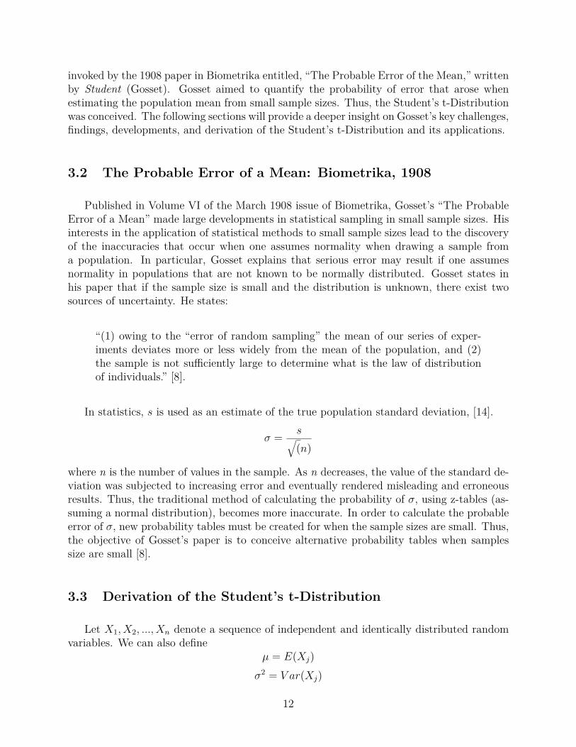
3.2 The Probable Error of a Mean: Biometrika, 1908

Published in Volume VI of the March 1908 issue of Biometrika, Gosset’s “The ProbableError of a Mean” made large developments in statistical sampling in small sample sizes. Hisinterests in the application of statistical methods to small sample sizes lead to the discoveryof the inaccuracies that occur when one assumes normality when drawing a sample froma population. In particular, Gosset explains that serious error may result if one assumesnormality in populations that are not known to be normally distributed. Gosset states inhis paper that if the sample size is small and the distribution is unknown, there exist twosources of uncertainty. He states:

“(1) owing to the “error of random sampling” the mean of our series of exper-iments deviates more or less widely from the mean of the population, and (2)the sample is not su�ciently large to determine what is the law of distributionof individuals.” [8].

In statistics, s is used as an estimate of the true population standard deviation, [14].

‡ = sÒ

(n)

where n is the number of values in the sample. As n decreases, the value of the standard de-viation was subjected to increasing error and eventually rendered misleading and erroneousresults. Thus, the traditional method of calculating the probability of ‡, using z-tables (as-suming a normal distribution), becomes more inaccurate. In order to calculate the probableerror of ‡, new probability tables must be created for when the sample sizes are small. Thus,the objective of Gosset’s paper is to conceive alternative probability tables when samplessize are small [8].

3.3 Derivation of the Student’s t-Distribution

Let X1, X2, ..., Xn

denote a sequence of independent and identically distributed randomvariables. We can also define

µ = E(Xj

)‡2 = V ar(X

j

)

12

, where Xj

≥ N(µ, ‡

2

n

) and j µ (1, 2, ..., n). We can then define our sample variance as

S2n

= 1n ≠ 1

Nÿ

n=1(X

j

≠ X̄n

)

We can also show thatZ = X̄

n

≠ µ‡Ôn

is normally distributed pivotal quantity with mean 0 and variance 1. A pivotal quantity isa function of observations and unobservable parameters whose probability distribution doesnot depend on unknown parameters. We know this because X̄

n

is normally distributed withmean µ and standard error ‡

n

. Gosset studied a related pivotal quantity that di�ered onlyby the standard deviation value. His pivotal quantity was defined as

T = X̄n

≠ µS

nÔn

[26]. Specifically, this pivotal quantity can be used to determine a t-score, which is necessaryin the calculation of p-values. In hypothesis testing, a p-value is required to determine thestatistical significance of your results. [27]

Furthermore, Gosset’s work was crucial in the derivation of the t-distribution’s probabilitydistribution function (p.d.f). In essence, the student’s t-distribution is derived by dividing anormally distributed random variable by a chi-squared distributed random variable. [17] Hestarted by defining the statistic variable t as

t = uÒ

v

n

where u is a variable of the standard normal distribution g(u), and v is a variable of thechi-squared distribution H

n

(v), with n degrees of freedom. As such, we can state t in termsof g(u) and H

n

(v), where both can be defined as follows:

g(u) = 1Ô2fi

e≠ u

22

Hn

(v) = 12n/2�(n/2)

The probabilistic function fn

(t) can then be defined as

fn

(t) =⁄

”(t ≠ uÒ

v

n

)g(u)Hn

(v)dudv

13

where ”(t ≠ uÔv

n

) is a Dirac’s delta function. A Dirac’s delta function is a generalizedfunction on the real number line that is zero everywhere except zero, with an integral of oneover the entire line. We will now integrate the above over y, where y = uÔ

v

n

. So,

fn

(t) =⁄ Ú

v

n”(t ≠ y)g(

Úv

ny)H

n

(v)dydv

fn

(t) =⁄ Ú

v

ng(

Úv

nt)H

n

(v)dv

by properties of the Dirac delta function.

Substituting our equation for g(u) into Hn

(v) into our integral, we get

fn

(t) = 1Ô2nfi2n/2�(n

2 )

⁄ Œ

0v

n≠12 e

≠(1+t

2)n

v

2 dv

We can rewrite our equation using a variable x = (1 + t

2

n

)v

2 instead of v, to find that

fn

(t) =(1 + t

2

n

)≠ n+12

Ônfi�(n

2 )

⁄ Œ

0x

n+12 ≠1e≠xdx

We can express our integrand using the Gamma Function, defined as

�(–) =⁄ Œ

0x–≠1e≠xdx

Thus, we obtain

fn

(t) =�(n+1

2 )Ônfi�(n

2 )(1 + t2

n)≠ n+1

2

We can use the Beta function B to represent Gamma functions as

B(12 ,

n

2 ) =�(1

2)�(n

2 )�(n+1

2 )

=Ô

fi�(n

2 )�(n+1

2 )

Finally, we obtain the pdf of Student’s t-Distribution as

fn

(t) = 1ÔnB(1

2 , n

2 )(1 + t2

n)≠ n+1

2

where t is an element of real numbers and n can take values of 1 onwards. [17]

We can also define E(T ) = 0 for r > 1 and V ar(T ) = r

r≠2 for r > 2, and Œ for 1 < r Æ 2[16].

14

Figure 1: The PDF of the Student’s t-Distribution [34]

3.3.1 Calculating E[T]

Let T be a random variable that follows the t-Distribution. From the above, we knowthat T has the probability density function

fn

(t) = 1ÔfiB(1

2 , n

2 )(1 + t2

n)≠ n+1

2

.

By definition, E[X] for a random variable X is defined as

E[X] =⁄ Œ

≠Œxf

x

(x)dx

where fx

(x) is the pdf of X. Thus,

E[T ] =⁄ Œ

≠Œtf

n

(t)dt

=⁄ Œ

≠Œt

1ÔnB(1

2 , n

2 )(1 + t2

n)≠ n+1

2 dt

= 1ÔnB(1

2 , n

2 )

⁄ Œ

≠Œt ú (1 + t2

n)≠ n+1

2 dt

Notice the function f(x) = x ú (1 + x

2

n

)≠ n+12 is an odd function since f(-x)=-f(x), so the

integral is 0.

Thus, E[T ] = 0.

15

3.3.2 Properties of the t-Distribution

Let f(t) be the pdf of the t-Distribution, with t being the degrees of freedom.

1. f(t) converges to N(0, 1) as the t æ Œ.

2. f is symmetric around t=0.

3. f has inflection points at ±Ò

(n/(n ≠ 1)).

4. f(t) æ 0 as t æ Œ and t æ ≠Œ. [24]

3.4 Student’s t-Test

The t-test is a statistical analysis of two population means. The t-test falls under the gen-eral category of hypothesis testing. As the name suggests, the t-test relies on the t-statistic,the t-distribution and degrees of freedom to determine the probability of the di�erence be-tween two population means. As opposed to the z-test, the t-test is used in hypothesistesting when n is relatively small (below 30, though this specific value can be argued) andmost importantly, when the population standard deviation is unknown. [28]

There are three situations in hypothesis testing where the t-test can be used. In general,when conducting a hypothesis test, a discrepancy measure must be calculated to determinean associated p-value. The p-value is then used to determine the validity of the hypothesis.Note, d is the discrepancy measure, µ0 refers to the population mean, µ̂ is the sample (withµ̂

x

and µ̂y

corresponding to means of samples x and y respectively), s is the sample stan-dard deviation and n is the number of units within a sample (with n

x

and ny

correspondingto sample counts for specified samples). [18] The discrepancy values for each situation areshown below:

1. Single sample mean tested against a known mean

d = µ̂ ≠ µ0sÔn

2. Comparison of means from two dependent samples

The formula for this situation is the same as the first case, except µ̂ is replaced by thedi�erence between the two sample means, and the denominator values are replaced by thedi�erence in the sample standard deviations divided by the number of units within eithersample (since both counts should be the same).

16

3. Comparison of means from two independent samples

d = µ̂x

≠ µ̂y

≠ µ0Ús

2x

n

x

+ s

2y

n

y

Note, for a problem requiring the analysis of three or more population groups, an ANOVA(Analysis of Variance) table should be used. [18]

3.5 Statistical Applications

3.5.1 Monte Carlo Analysis

The Monte Carlo analysis falls under the category of statistical simulation tools. It al-lows one to simulate data sets and compare the di�erences and similarities of parameters ofinterest between the sets. [18]

The simulation works by building models of possible results through a range of acceptablevalues for any factor that has inherent uncertainty. Essentially, a probability distributionis built with these values. Values of interest are then calculated over and over again, eachtime using a di�erent set of random values from the probability functions. Depending on thenumber of uncertainties and the ranges specified for them, a Monte Carlo simulation couldinvolve tens or thousands of recalculations before it is complete.[16] As implied, the proba-bility distribution of the data is required to be known before this technique can be performed.

The t-test comes in to play when we wish to check the di�erence between two setsof simulated values. Specifically, we can calculate the mean of two sets of simulated valuesand perform a hypothesis test to check if the di�erence between the two means is 0 (i.e. dothe parameters of interest from the two groups di�er). [16]

The t-test does not play a role in the actual simulation of data. However, it can beused to verify results of simulations, as with the Monte Carlo. This application of the t-testis not specific to Monte Carlo simulation, but to many forms of statistical simulation.

3.5.2 Confidence Intervals

As aforementioned, the purpose of surveying a random sample from a population andcomputing a statistical measure (i.e. mean, standard deviation, or variance) is to approx-imate such statistical measures of the true population. As previously discussed, how wella statistic derived from a sample size estimates the true population value is an variable indetermining the power of the study.

17

Definition 3: A 100p% confidence interval for a parameter is an interval estimate[L(y), U(y)] for which

P [L(Y ) Æ ◊ Æ U(Y )] = p

where p is called the confidence coe�cient [14].

The confidence interval addresses the issue, as it provides a range of values which islikely to contain the true population statistic [21]. Confidence intervals are constructed at apredetermined confident coe�cient, with p = 0.95 (95%) being the most common. A 95%confidence interval suggests that if repeated samples were taken and a confidence interval wascreated on each occasion, the true population statistic would be contained in the intervals95% of the time [13].

Gosset recognized that small sample sizes produce wider intervals and inaccuracies. Ifthe the margin of error is wished to be reduced by 50%, the sample size must be increasedby 250%. To calculate the confidence interval; if one draws a simple random sample of size nfrom a population that is approximately normally distributed with mean µ and an unknownstandard deviation ‡, and calculated the t-statistic. Then, t-statistic follows a Student’st-Distribution with n ≠ 1 degrees of freedom [7].

The confidence interval for the mean µ of a sample size using the Student’s t-Distributionis given by [30]:

x̄ ± t( sÔn

)

3.6 Sample Problems

Example 1: Hypothesis Testing

Suppose we attain a set of data whereby male university students measure their pulserates. Is the pulse rate for 25 university males equal to 70? Note that key statistics aresummarized below.

Figure 2: Summary Statistics

18

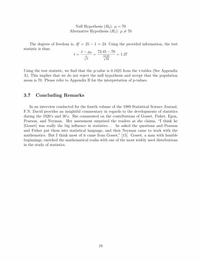
Null Hypothesis (H0): µ = 70Alternative Hypothesis (H1): µ ”= 70

The degrees of freedom is, df = 25 ≠ 1 = 24. Using the provided information, the teststatistic is thus:

t = x̄ ≠ µ0sÔn

= 73.45 ≠ 7012.31Ô

24= 1.37

Using the test statistic, we find that the p-value is 0.1825 from the t-tables (See AppendixA). This implies that we do not reject the null hypothesis and accept that the populationmean is 70. Please refer to Appendix B for the interpretation of p-values.

3.7 Concluding Remarks

In an interview conducted for the fourth volume of the 1989 Statistical Science Journal,F.N. David provides an insightful commentary in regards to the developments of statisticsduring the 1920’s and 30’s. She commented on the contributions of Gosset, Fisher, Egon,Pearson, and Neyman. Her assessment surprised the readers as she claims, “I think he[Gosset] was really the big influence in statistics. . . he asked the questions and Pearsonand Fisher put them into statistical language, and then Neyman came to work with themathematics. But I think most of it came from Gosset.” [15]. Gosset, a man with humblebeginnings, enriched the mathematical realm with one of the most widely used distributionsin the study of statistics.

19

APPENDIX

Appendix A: Student t Quantiles (t-table)

Figure 3: t-table [14]

20

Appendix B: Interpretation of p-values

Figure 4: Interpretation of p-vales [14]

21

References

[1] Andale. (2017). “Sample Sizes in Statistics: How to Find it”. Statistics How To, http://www.statisticshowto.com/find-sample-size-statistics/, Accessed 18 June 2017.

[2] “Archive Fact Sheet: Employee Welfare at Guinness.” Guinness Storehouse,https://www.guinness-storehouse.com/content/pdf/archive-factsheets/guinness-philanthropy/employee_welfare_at_guinness.pdf. Accessed 12 June2017.

[3] “Archive Fact Sheet: The History of Guinness.” Guinness Storehouse,https://www.guinness-storehouse.com/content/pdf/archive-factsheets/general-history/company-history.pdf. Accessed 5 June 2017.

[4] “Beer.” The Merriam-Webster Dictionary. Online, https://www.merriam-webster.com/dictionary/beer. Accessed 18 June 2017.

[5] Boland, P.J. “A Biographical Glimpse of William Sealy Gosset”, 9 Jan 2008,https://www.jstor.org/stable/pdf/2683648.pdf?refreqid=excelsior:3b99\8c401ca85bf030770afb8ecb369c. Accessed 19 June 2017.

[6] Box, J. F. (1987). Guinness, Gosset, Fisher, and Small Samples. Statistical Science,2(1), 45-52, http://www2.fiu.edu/~blissl/GuinessGossetFisher.pdf. Accessed 19June 2017.

[7] Dean, Susan et al. (2008). “Confidence Intervals: Confidence Interval, Single Popula-tion Mean, Standard Deviation Unknown, Student’s-t”. Openstax, http://cnx.org/contents/PYKzWbZZ@24/Confidence-Intervals-Confidenc. Accessed 17 June 2017.

[8] Gosset, W. (1908). Biometrika, pp.1-25, reprinted on pp. 11-34 in “Student’s” Col-lected Papers, Edited by E.S. Pearson and John Wishart with a Foreword by LaunceMcMullen, Cambridge University Press for the Biometrika Trustees, 1942

[9] “Gosset, William Sealy.” International Encyclopedia of the Social Sciences, Encyclope-dia.com, 19 June 2017, www.encyclopedia.com/people/social-sciences-and-law/sociology-biographies/william-sealy-gosset. Accessed 19 June 2017.

[10] Guinness. (2006). “Our Story”. Guinness, https://www.guinness.com/en-ca/our-story/. Accessed 17 June 2017.

[11] Guinness Storehouse. (2017). “FAQ”. Guinness Storehouse, https://www.guinness-storehouse.com/en/faq. Accessed 23 June 2017.

[12] Investopedia. (n.d). “Sampling Error”. Investopedia, http://www.investopedia.com/terms/s/samplingerror.asp. Accessed 19 June 2017.

[13] Lane, David. “Confidence Intervals Introduction”. Online Stat Book, http://onlinestatbook.com/2/estimation/confidence.html. Accessed 18 June 2017.

22

[14] Lawless, Jerry. (2013) Statistics 231 Course Notes Spring 2013. Waterloo: University ofWaterloo, 2013. Print.

[15] Lehmann, E.L. “‘Student’ and Small-Sample Theory”. University of California, Berke-ley, http://statistics.berkeley.edu/sites/default/files/tech-reports/541.pdf. Accessed 19 June 2017.

[16] “Monte Carlo Simulation: What Is It and How Does It Work? - Palisade.” Parlisade,www.palisade.com/risk/monte_carlo_simulation.asp. Accessed 17 June 2017.

[17] Midorikawa, Shoichi. “Derivation of the t-Distribution.” Https://Shoichimidorikawa.github.io/Lec/ProbDistr/t-E.pdf. Accessed 15 June 2017.

[18] Metzger, Riley. STAT 340 Simulation with R. Spring 2016 ed., Waterloo, ON, Universityof Waterloo, 2015.

[19] Meussdoer�er, Franz G. “A Comprehensive History of Beer Brewing”. Handbookof Brewing: Processes, Technology, Markets. Ed. H. M. Eblinger. WILEY-VCHVerlag GmbH & Co, 2009, https://application.wiley-vch.de/books/sample/3527316744_c01.pdf, Accessed 17 June 2017.

[20] Mark, Joshua J. (2011). “The Hymn to Ninkasi, Goddess of Beer”. Ancient HistoryEncyclopedia. http://www.ancient.eu/article/222/. Accessed 23 June 2017.

[21] Nist Sematech. (n.d). “What are confidence intervals?”. Nist Sematech, http://www.itl.nist.gov/div898/handbook/prc/section1/prc14.htm. Accessed 17 June 2017.

[22] The Pennslyvania State University. (2007). “Hypothesis Testing for a Mean”. The Penn-sylvania State University, http://sites.stat.psu.edu/~ajw13/stat200_notes/09_hypoth/04_hypoth_mean.htm. Accessed 18 June 2017

[23] Raju, Tonse N. “William Sealy Gosset and William A. Silverman: Two “Students” ofScience.” Pediatrics, vol. 116, no. 3, 3 Sept. 2005.

[24] Siegrist, Kyle. “The Student t-Distribution.” The Student t Distribution, www.math.uah.edu/stat/special/Student.html. Accessed 20 June 2017.

[25] Statistics Solutions. (2017). “Sample Size Formula”. Statistics Solutions, http://www.statisticssolutions.com/sample-size-formula/. Accessed 18 June 2017.

[26] “Student’s t-Distribution.” Mcgill, http://www.cs.mcgill.ca/~rwest/link-suggestion/wpcd_2008-09_augmented/wp/s/Student%2527s_t-distribution.htm. Accessed 17 June 2017.

[27] “Student’s t-Distribution.” Wolfram MathWorld, mathworld.wolfram.com/Studentst-Distribution.html. Accessed 15 June 2017.

[28] “T Test (Student’s T-Test): Definition and Examples.” Statistics How To, www.statisticshowto.com/t-test/#ttest1. Accessed 16 June 2017.

23

[29] Verial, Damon. (2017). “The E�ect of a Small Sample Size Limitation”. Sciencing,http://sciencing.com/effects-small-sample-size-limitation-8545371.html.Accessed 17 June 2017.

[30] Western Michigan University, “t-based Confidence Interval for the Mean”. West-ern Michigan University, http://www.stat.wmich.edu/s216/book/node79.html. Ac-cessed 19 June 2017.

[31] Wikipedia. “Alcoholic drink.” Wikipedia. Wikimedia Foundation, 18 June 2017, https://en.wikipedia.org/wiki/Alcoholic_drink. Accessed 19 June 2017

[32] Wikipedia. “Karl Pearson.” Wikipedia. Wikimedia Foundation, 19 June 2017, https://en.wikipedia.org/wiki/Karl_Pearson. Accessed 19 June 2017.

[33] Wikipedia. “Ronald Fisher.” Wikipedia, Wikimedia Foundation, 18 June 2017, en.wikipedia.org/wiki/Ronald_Fisher. Accessed 19 June 2017.

[34] Wikipedia. “Student’s t-Distribution.” Wikipedia, Wikimedia Foundation, 18 June 2017,https://en.wikipedia.org/wiki/Student%27s_t-distribution. Accessed 19 June2017

[35] Ziliak, Stephen T. “Great Lease, Arthur Guinness—Lovely Day for a Gos-set! .” Stephen T Ziliak, September 2009, stephentziliak.com/doc/Beeronomics%20issue-Ziliak%20article-Great%20Lease%20Arthur%20Guinness%20JWE.pdf. Ac-cessed 19 June 2017.

24