Stat 529 (Winter 2011)

Analysis of Variance (ANOVA)

Reading: Sections 5.1–5.3.

• Introduction and notation

– Birthweight example

– Disadvantages of using many pooled t procedures

• The analysis of variance procedure

– Assumptions

– The hypothesis test

– The sampling distribution of the sample means

– The variability between the sample means

∗ Is there any difference in the means?

– Estimating σ2

– The F test statistic and F distribution

– Performing the ANOVA for the birthweight data

1

Introduction

• We move away from comparing two populations means, on

the basis of data drawn from each population.

– Now we consider multiple populations.

• Here are some motivating examples:

1. There are three methods of assessing a concentration of a

contaminant in water. Are all three methods equivalent?

2. How does the paper thickness vary for five different pro-

duction lines?

3. How is the average crop yield affected by the use of four

different fertilizers?

2

Notation

• Suppose that we have I samples drawn from I populations.

• For each population i = 1, . . . , I we have:

µi : mean of population i.

σ2i : variance of population i.

• We draw ni observations from population i:

Yij : the jth observation within population i.

In total we have n1 + . . . + nI = n observations.

• Estimates of µi and σ2i are respectively

Y i : sample mean for sample i, and

s2i : sample variance for sample i.

3

Birthweights example

One measure of the overall health of a newborn baby is its birth-

weight. There are many factors which affect birthweight, in-

cluding both genetic factors (such as mother’s size or mother’s

birthweight) and environmental factors. One environmental fac-

tor which is believed to lower birthweight is maternal smoking.

The data below present birthweights of a small number of infants,

with the mother’s smoking status during pregnancy recorded as

non-smoker (someone who has never smoked), former smoker,

light smoker or heavy smoker. Birthweight is recorded in pounds,

with the ounces part translated into a decimal.

Non Quit Light Heavy

7.5 5.8 5.9 6.2

6.2 7.3 6.2 6.8

6.9 8.2 5.8 5.7

7.4 7.1 4.7 4.9

9.2 7.8 8.3 6.2

8.3 7.2 7.1

7.6 6.2 5.8

5.4

4

Birthweights: questions of interest

• The question of primary concern is whether a mother’s smok-

ing reduces the mean birthweight of an infant. Two issues to

consider when performing an analysis are:

1. We would like to make use of all of the information in our

data.

2. We would like to avoid performing so many analyses on

our data that we find “significant differences” where there

are none.

5

Summaries of the data

Maternal

smoking

Variable status N Mean SE Mean StDev Variance Minimum

Birthweight in pounds Heavy 8 6.013 0.255 0.720 0.518 4.900

Light 7 6.329 0.431 1.140 1.299 4.700

Non 7 7.586 0.363 0.962 0.925 6.200

Quit 5 7.240 0.408 0.913 0.833 5.800

Variable status Q1 Median Q3 Maximum IQR

Birthweight in pounds Heavy 5.475 6.000 6.650 7.100 1.175

Light 5.800 6.200 7.200 8.300 1.400

Non 6.900 7.500 8.300 9.200 1.400

Quit 6.450 7.300 8.000 8.200 1.550

6

Discussion of the summaries

7

Many pooled t procedures

• We could make all the 6 pairwise comparisons of the means:

µ1 − µ2, µ1 − µ3, µ1 − µ4,

µ2 − µ3, µ2 − µ4, µ3 − µ4.

• Based on the results of many pooled t-tests, we might con-

clude that “maternal smoking is related to lower birthweight”.

• Disadvantages:

1. If the additive model holds and all the variances are equal

then why do we use six different estimates of σ2, with

differing degrees of freedom? Should we not pool all the

information about the variability from all the samples?

2. Then chance of making at least one I type error in

all the tests of µi − µj is larger.

e.g., For 6 tests, the chance of making at least one type I

error in all six tests lies between α and 6α.

(in our case between 0.05 and 0.30).

8

The analysis of variance procedure

• The ANalysis Of VAriance (ANOVA) procedure tries to rem-

edy all these problems (it certainly fixes 2.)

• Assume that the additive model is appropriate for each of our

I samples.

• Our model is

Yij = µi + εij.

• Here µi is the mean of population i and εij is the “error”.

– We assume the errors are

• Then Yij are

9

Assumptions

• Y11, . . . , Y1n1 form a random sample from some population.

Y21, . . . , Y2n2 form a random sample from a second popula-

tion.

Similarly, further samples are random samples from some

population.

With I samples, the last sample is YI1, . . . , YInI.

• The I samples are independent of one another.

• The population distributions are normal with unknown means

µ1, µ2, . . . , µI and with a common unknown standard de-

viation σ.

10

The hypothesis test

• The null hypothesis in ANOVA is “no difference”. That is,

H0 : µ1 = µ2 = . . . = µI .

• The alternative is “not H0”, or more specifically

Ha : at least two of the means differ,

which is the same as

Ha : there is some difference in the means.

• Our test is based on measuring how far apart the sample

means are from one another.

– The further they are apart the more likely we will be to

reject H0.

11

The sampling distribution of the sample means

• For each population i the distribution of each Y i is

• Since the observations are independent across populations,

• Under H0 : µ1 = µ2 = . . . = µI = µ, say, the distribution of

Y i is

• Then under H0 an estimate for µ, the common or grand

mean, is

12

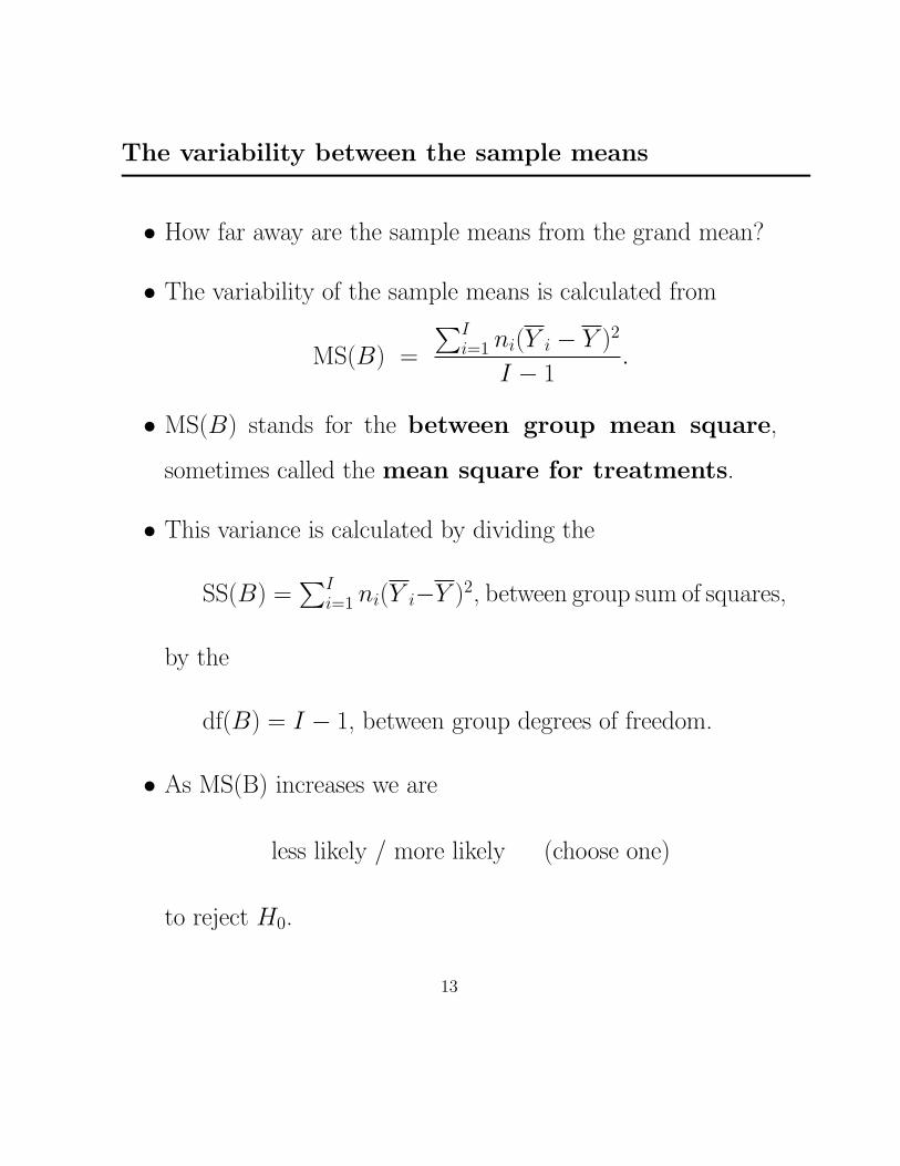
The variability between the sample means

• How far away are the sample means from the grand mean?

• The variability of the sample means is calculated from

MS(B) =

∑Ii=1 ni(Y i − Y )2

I − 1.

• MS(B) stands for the between group mean square,

sometimes called the mean square for treatments.

• This variance is calculated by dividing the

SS(B) =∑I

i=1 ni(Y i−Y )2, between group sum of squares,

by the

df(B) = I − 1, between group degrees of freedom.

• As MS(B) increases we are

less likely / more likely (choose one)

to reject H0.

13

Birthweights example: calculating MS(B)

(Exercise: check this for yourself!)

• In total there are n =∑

i ni = 8+7+7+5 = 27 observations.

• The grand mean, calculated from the summary statistics is

Y =

∑i

∑j Yij

n=

∑i niY i

n

=8× 6.013 + 7× 6.329 + 7× 7.586 + 5× 7.240

27

=181.709

27= 6.73.

• Thus

SS(B) =∑i

ni(Y i − Y )2

= 8× (6.013− 6.73)2 + 7× (6.329− 6.73)2 +

7× (7.586− 6.73)2 + 5× (7.240− 6.73)2 = 11.667,

df (B) =

and

MS(B) =SS(B)

df (B)=

14

How large should MS(B) be?

• We compare MS(B) to σ2, the variance within the samples.

– We need to estimate σ2 .

• For each population i, we know that s2i is an estimate of σ2.

• Pooling across the populations, an estimate of σ2 is

MS(W ) = s2p =

(n1 − 1)s21 + . . . + (nI − 1)s2

I

(n1 − 1) + . . . + (nI − 1)

=

∑Ii=1(ni − 1)s2

i

n− I.

• This is called the within group mean square, or the

mean square for the error.

• This variance is calculated by dividing the

SS(W ) =∑I

i=1(ni − 1)s2i , within group sum of squares,

by the

df(W ) = n− I , within group degrees of freedom.

15

Birthweights example: calculating MS(W)

(Exercise: check this for yourself!)

• We have that

SS(W ) =∑i

(ni − 1)s2i

= 7× 0.518 + 6× 1.299 +

6× 0.925 + 4× 0.833 = 20.302

df (W ) =

and

MS(W ) =SS(W )

df (W )=

16

The F test statistic

• Under the additive model with normal populations with H0 :

µ1 = µ2 = . . . = µI being true, the F test statistic,

F =MS(B)

MS(W ),

follows an F distribution with

df(B) = I − 1 numerator degrees of freedom,

and

df(W ) = n− I denominator degrees of freedom.

• We reject H0 for large values of the observed F statistic,

Fobs. The p-value is

P (F ≥ Fobs),

where F is a F distributed random variable on I − 1 and

n− I df.

17

Viewing the F distribution

• The F distribution has two separate degrees of freedom.

• It is a positive and right skewed distribution.

• Some of the critical values are tabulated in Table A.4 (p.720–

727).

– Can also use MINITAB to directly calculate the p-value.

0 1 2 3 4 5 6

0.0

0.1

0.2

0.3

0.4

0.5

0.6

0.7

dens

ity fo

r F

on

3 an

d 23

df

18

Finding the p-value for an F-test in MINITAB

• Calc → Probability Distributions → F.

– Check Cumulative Probability, and use the default

value of 0.0 for Noncentrality parameter.

– Specify the numerator and denominator degrees of free-

dom in the corresponding boxes.

– Highlight Input Constant and enter the value of the

F-statistic, Fobs.

– Leave Optional Storage blank.

• Minitab’s output gives P (F ≤ Fobs), but the p-value is

P (F ≥ Fobs) = 1 − P (F < Fobs) = 1 − P (F ≤ Fobs)

(since the F distribution is continuous).

19

Birthweights example: Performing the ANOVA test

20

Carrying out the test in MINITAB

• Stat → ANOVA → One-Way

– Response: Weight in pounds

– Factor: Reduced Maternal Status

– Click OK

One-way ANOVA: Birthweight in pounds versus Maternal smoking status

Source DF SS MS F P

Maternal smoking 3 11.673 3.891 4.41 0.014

Error 23 20.304 0.883

Total 26 31.976

S = 0.9396 R-Sq = 36.50% R-Sq(adj) = 28.22%

Individual 95% CIs For Mean Based on Pooled StDev

Level N Mean StDev ---+---------+---------+---------+------

Heavy 8 6.0125 0.7200 (-------*--------)

Light 7 6.3286 1.1398 (--------*--------)

Non 7 7.5857 0.9616 (--------*--------)

Quit 5 7.2400 0.9127 (---------*----------)

---+---------+---------+---------+------

5.60 6.40 7.20 8.00

Pooled StDev = 0.9396

21

The analysis of variance table

One-way ANOVA: Birthweight in pounds versus Maternal smoking status

Source DF SS MS F P

Maternal smoking 3 11.673 3.891 4.41 0.014

Error 23 20.304 0.883

Total 26 31.976

• An analysis of variance table lists all the sources of

variability that we account for in our data:

1. The variability within the groups (treatments)

– Maternal smoking for our example.

2. The variability between the groups (errors).

3. The total variability.

• It is an easy way to lay out the F test of

H0: µ1 = . . . = µI , versus

Ha: there is some difference in the means.

22

The layout of the analysis of variance table

Sum of Mean

Source d.f. Squares Squares F Statistic p-value

Between groups I − 1 SS(B) MS(B) Fobs P (F ≥ Fobs)

Within groups n− I SS(W) MS(W)

Total n− 1 SS(T)

23

More of the MINITAB output

S = 0.9396 R-Sq = 36.50% R-Sq(adj) = 28.22%

• S is the pooled estimate of the S.D., sp =√MS(W ).

– For the birthweights, sp =√

0.883 = 0.9396.

• R-Sq, R2, is the percentage of the total variance accounted

for by the model:

R2 =SS(B)

SS(T )× 100%.

• For the birthweights it is

R2 =SS(B)

SS(T )× 100% =

11.673

20.304× 100% = 28.22%.

• For Stat 529, ignore R-Sq(adj).

24

CIs for each population mean, differences of means

Individual 95% CIs For Mean Based on Pooled StDev

Level N Mean StDev ---+---------+---------+---------+------

Heavy 8 6.0125 0.7200 (-------*--------)

Light 7 6.3286 1.1398 (--------*--------)

Non 7 7.5857 0.9616 (--------*--------)

Quit 5 7.2400 0.9127 (---------*----------)

---+---------+---------+---------+------

5.60 6.40 7.20 8.00

Pooled StDev = 0.9396

• Using the pooled estimate of the S.D., sp,

a 100(1− α)% CI for µi is given by

Y i ± tn−I(1− α2 )

sp√ni.

• A 100(1−α)% CI for µi−µj (i 6= j) can be calculated using

Y i − Y j ± tn−I(1− α2 )sp

√1

ni+

1

nj.

• These intervals do not adjust for making multiple compar-

isons (we will correct for multiple comparisons later in the

course).

25