SPACECRAFT CHARGING MODELING NASCAP- 2K · San Diego, CA 92121 . 21 September 2012 . ... Spacecraft Charging Modeling—Nascap-2k contract is to develop, ... Standard Form 298

AFRL-RV-PS- AFRL-RV-PS- TR-2012-0209 TR-2012-0209

SPACECRAFT CHARGING MODELING – NASCAP-2K V. A. Davis M. J. Mandell Science Applications International Corporation 10260 Campus Point Drive, Mailstop A-2A San Diego, CA 92121 21 September 2012

Technical Report

APPROVED FOR PUBLIC RELEASE; DISTRIBUTION IS UNLIMITED.

AIR FORCE RESEARCH LABORATORY Space Vehicles Directorate 3550 Aberdeen Ave SE AIR FORCE MATERIEL COMMAND KIRTLAND AIR FORCE BASE, NM 87117-5776

Approved for public release; distribution is unlimited.

DTIC COPY

NOTICE AND SIGNATURE PAGE Using Government drawings, specifications, or other data included in this document for any purpose other than Government procurement does not in any way obligate the U.S. Government. The fact that the Government formulated or supplied the drawings, specifications, or other data does not license the holder or any other person or corporation; or convey any rights or permission to manufacture, use, or sell any patented invention that may relate to them. This report was cleared for public release by the 377 ABW Public Affairs Office and is available to the general public, including foreign nationals. Copies may be obtained from the Defense Technical Information Center (DTIC) (http://www.dtic.mil). AFRL-RV-PS-TR-2012-0209 HAS BEEN REVIEWED AND IS APPROVED FOR PUBLICATION IN ACCORDANCE WITH ASSIGNED DISTRIBUTION STATEMENT. //signed// //signed// ________________________________________ _______________________________________ Adrian Wheelock Edward J. Masterson, Colonel, USAF Project Manager, AFRL/RVBXR Chief, AFRL/RVB This report is published in the interest of scientific and technical information exchange, and its publication does not constitute the Government’s approval or disapproval of its ideas or findings.

REPORT DOCUMENTATION PAGE Form Approved

OMB No. 0704-0188 Public reporting burden for this collection of information is estimated to average 1 hour per response, including the time for reviewing instructions, searching existing data sources, gathering and maintaining the data needed, and completing and reviewing this collection of information. Send comments regarding this burden estimate or any other aspect of this collection of information, including suggestions for reducing this burden to Department of Defense, Washington Headquarters Services, Directorate for Information Operations and Reports (0704-0188), 1215 Jefferson Davis Highway, Suite 1204, Arlington, VA 22202-4302. Respondents should be aware that notwithstanding any other provision of law, no person shall be subject to any penalty for failing to comply with a collection of information if it does not display a currently valid OMB control number. PLEASE DO NOT RETURN YOUR FORM TO

THE ABOVE ADDRESS. 1. REPORT DATE (DD-MM-YYYY) 21-09-2012

2. REPORT TYPE Technical Report

3. DATES COVERED (From - To) 19 Sep 2011 – 21 Sep 2012

4. TITLE AND SUBTITLE

5a. CONTRACT NUMBER

FA9453-11-C-0262 Spacecraft Charging Modeling—Nascap-2k 5b. GRANT NUMBER

5c. PROGRAM ELEMENT NUMBER

63601F 6. AUTHOR(S)

5d. PROJECT NUMBER

1010 V.A. Davis M.J. Mandell

5e. TASK NUMBER

PPM00012836

5f. WORK UNIT NUMBER EF003277 7. PERFORMING ORGANIZATION NAME(S) AND ADDRESS(ES)

8. PERFORMING ORGANIZATION REPORT

NUMBER Science Applications International Corporation 10260 Campus Point Drive, Mailstop A-2A San Diego, CA 92121

9. SPONSORING / MONITORING AGENCY NAME(S) AND ADDRESS(ES) 10. SPONSOR/MONITOR’S ACRONYM(S) Air Force Research Laboratory

Space Vehicles Directorate AFRL/RVBXT 3550 Aberdeen Ave. SE 11. SPONSOR/MONITOR’S REPORT Kirtland AFB, NM 87117-5776 NUMBER(S) AFRL-RV-PS-TR-2012-0209 12. DISTRIBUTION / AVAILABILITY STATEMENT

Approved for public release; distribution is unlimited. (377ABW-2012-1443 dtd 6 Nov 2012)

13. SUPPLEMENTARY NOTES

14. ABSTRACT In support of the larger goal to provide a plasma engineering capability to the spacecraft community, the objective of the Spacecraft Charging Modeling—Nascap-2k contract is to develop, incorporate, test, and validate new algorithms for the three-dimensional plasma-environment spacecraft interactions computational tool, Nascap-2k. Nascap-2k is being modified to extend the range of plasma physics phenomena that the code can simulate, make the advanced code capabilities more accessible to users, and improve and maintain both the graphical and non-graphical interfaces to the code. The upgraded code is being used to simulate problems of interest to AFRL. During the first year, Nascap-2k 4.1 was modified to specify, and then optionally use, a time-dependent tabular environment in surface charging calculations. The pseudopotential technique to compute volume electron currents was modified to use a finite element approach and to include the magnetic field dependence. The upgraded code is being used to support the DSX (Demonstration and Science eXperiments) and AEHF-2 (Advanced Extremely High Frequency) spacecraft programs. 15. SUBJECT TERMS Nascap-2k, Potentials, Space Environment, Spacecraft, Spacecraft Charging, DSX

16. SECURITY CLASSIFICATION OF:

17. LIMITATION

OF ABSTRACT

18. NUMBER

OF PAGES

19a. NAME OF RESPONSIBLE PERSON Adrian T. Wheelock

a. REPORT

Unclassified b. ABSTRACT Unclassified

c. THIS PAGE Unclassified

Unlimited

19b. TELEPHONE NUMBER (include area

code) Standard Form 298 (Rev. 8-98)

Prescribed by ANSI Std. 239.18

48

This page is intentionally left blank.

Approved for Public Release; Distribution is Unlimited.

i Approved for public release; distribution is unlimited.

TABLE OF CONTENTS

Page

LIST OF FIGURES ....................................................................................................................... iii

LIST OF TABLES ...........................................................................................................................v

1. INTRODUCTION .....................................................................................................................1

1.1. First Year Progress ........................................................................................................... 1

1.1.1. Interoperability of Nascap-2k with Other Codes ................................................. 1

1.1.2. Research Models of Spacecraft Charging and Discharging ................................. 2

1.1.3. Maintenance and Support .................................................................................... 2

1.1.4. Apply Nascap-2k to DSX .................................................................................... 3

1.1.5. Advanced EHF Analysis ...................................................................................... 4

1.1.6. Nascap-2k Enhancements Funded by Other Organizations ................................. 4

1.2. Reports and Meetings ...................................................................................................... 5

1.3. Scientific Reports and Journal Articles ............................................................................ 5

1.4. Personnel .......................................................................................................................... 6

2. MULTISITE DEVELOPMENT PLAN .....................................................................................7

3. DSX NEAR FIELD ANALYSIS ROADMAP ..........................................................................8

4. DSX ANTENNA IMPEDANCE FROM NASCAP-2K CALCULATIONS—FIRST ESTIMATE .............................................................................................................................. 11

4.1. Equations and Integrals .................................................................................................. 11

4.2. Vacuum Solution ............................................................................................................ 13

4.3. Plasma Solution ............................................................................................................. 14

5. MATERIAL PROPERTIES FITTING TOOL .........................................................................17

6. HYBRID PIC CHARGE DENSITY MODEL ........................................................................18

7. FINITE ELEMENT PSEUDOPOTENTIAL TREATMENT FOR NASCAP-2K ELECTRON CURRENTS .......................................................................................................20

7.1. Introduction .................................................................................................................... 20

7.2. Finite Element Formulation ........................................................................................... 20

7.3. Boundary Conditions ..................................................................................................... 22

7.3.1. Inner Boundary Conditions (Object Currents) ................................................... 22

7.3.2. Outer Boundary Conditions ............................................................................... 22

7.4. Grid Interface ................................................................................................................. 22

7.5. Conductivity Tensor ....................................................................................................... 23

7.6. Example ......................................................................................................................... 23

ii Approved for public release; distribution is unlimited.

7.7. Conclusions .................................................................................................................... 35

REFERENCES ..............................................................................................................................36

iii Approved for public release; distribution is unlimited.

LIST OF FIGURES

Page

Figure 1. Surface Potentials as a Function of Time for Vacuum Case at 10 kHz ..........................13

Figure 2. Injected Current Computed from Potentials in Figure 1 Compared with the Injected Current Computed from the Integral ................................................................................14

Figure 3. Antenna Injected Current in a 108 Plasma at 10 kHz .....................................................15

Figure 4. Antenna Injected Current in a 109 Plasma at 12 kHz .....................................................16

Figure 5. Antenna Injected Current in a 109 Plasma at 2 kHz .......................................................16

Figure 6. Material Properties Fitting Tool .....................................................................................17

Figure 7. Space Potentials Resulting from Nascap-2k Hybrid PIC Calculation of JAXA Wake Experiment with (left) and without (right) Charge Stabilization .........................................18

Figure 8. Ion Densities Resulting from Nascap-2k Hybrid PIC Calculation of JAXA Wake Experiment Computed with (left) and without (right) Charge Stabilization .......................19

Figure 9. Space Potentials and Ion Densities Resulting from Nascap-2k Hybrid PIC Calculation of JAXA Wake Experiment Using Revised Charge Stabilization Algorithm .............19

Figure 10. Bias Applied to Sphere .................................................................................................24

Figure 11. Electron Current Magnitude (B=0, 1 Grid) in X = 0 Plane ..........................................26

Figure 12. Z-component of Electron Current (B=0, 1 Grid) in X = 0 Plane .................................26

Figure 13. Electron Current Magnitude (B=0, Two Grids) in X = 0 Plane ...................................27

Figure 14. Z-component of Electron Current (B=0, 2 Grids) in X = 0 Plane ................................27

Figure 15. Z-component of Current (B=0, 1 Grid) When the Sphere is Collecting Electrons from the Plasma .............................................................................................................28

Figure 16. Magnitude of Current Density with Magnetic Field (B=(0.0, 0.0, 1.0×10-5), One Grid) in X = 0 Plane ...............................................................................................................29

Figure 17. Z-component of Current Density with Magnetic Field (B=(0.0, 0.0, 1.0×10-5), One Grid) in X = 0 Plane ...............................................................................................................29

Figure 18. X-Component of Current Density (Hall Current) with Magnetic Field (B=(0.0, 0.0, 1.0×10-5), One Grid) in X = 0 Plane ......................................................................................30

iv Approved for public release; distribution is unlimited.

Figure 19. Magnitude of Current Density with Magnetic Field (B=(0.0, 0.0, 1.0×10-5), Two Grids) in X = 0 Plane .............................................................................................................30

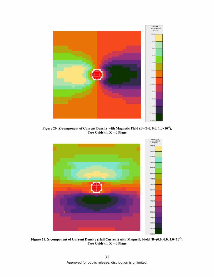
Figure 20. Z-component of Current Density with Magnetic Field (B=(0.0, 0.0, 1.0×10-5), Two Grids) in X = 0 Plane .............................................................................................................31

Figure 21. X-component of Current Density (Hall Current) with Magnetic Field (B=(0.0, 0.0, 1.0×10-5), Two Grids) in X = 0 Plane ....................................................................................31

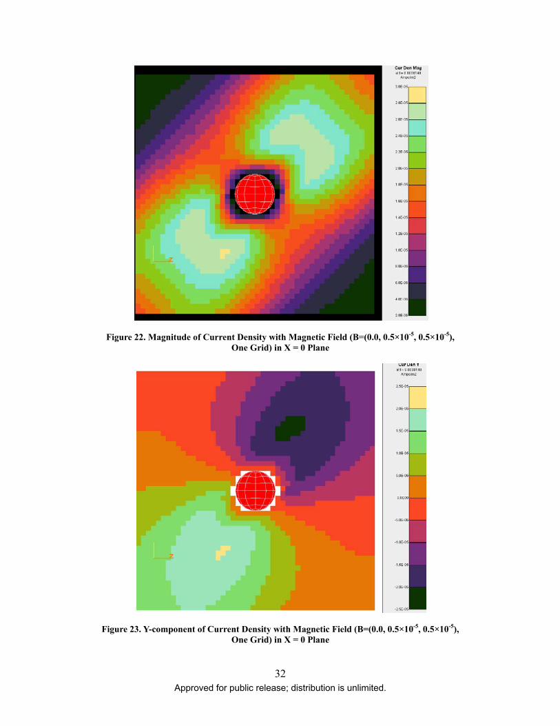
Figure 22. Magnitude of Current Density with Magnetic Field (B=(0.0, 0.5×10-5, 0.5×10-5), One Grid) in X = 0 Plane .............................................................................................32

Figure 23. Y-component of Current Density with Magnetic Field (B=(0.0, 0.5×10-5, 0.5×10-5), One Grid) in X = 0 Plane .............................................................................................32

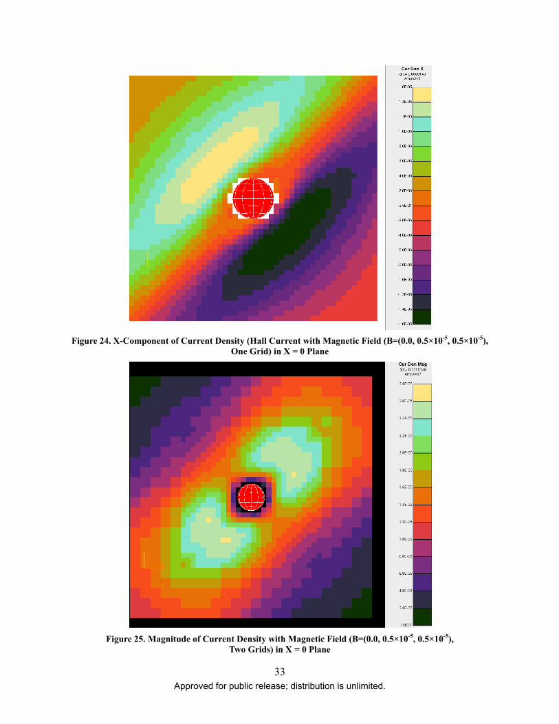
Figure 24. X-Component of Current Density (Hall Current with Magnetic Field (B=(0.0, 0.5×10-5, 0.5×10-5), One Grid) in X = 0 Plane ...............................................................................33

Figure 25. Magnitude of Current Density with Magnetic Field (B=(0.0, 0.5×10-5, 0.5×10-5), Two Grids) in X = 0 Plane ...........................................................................................33

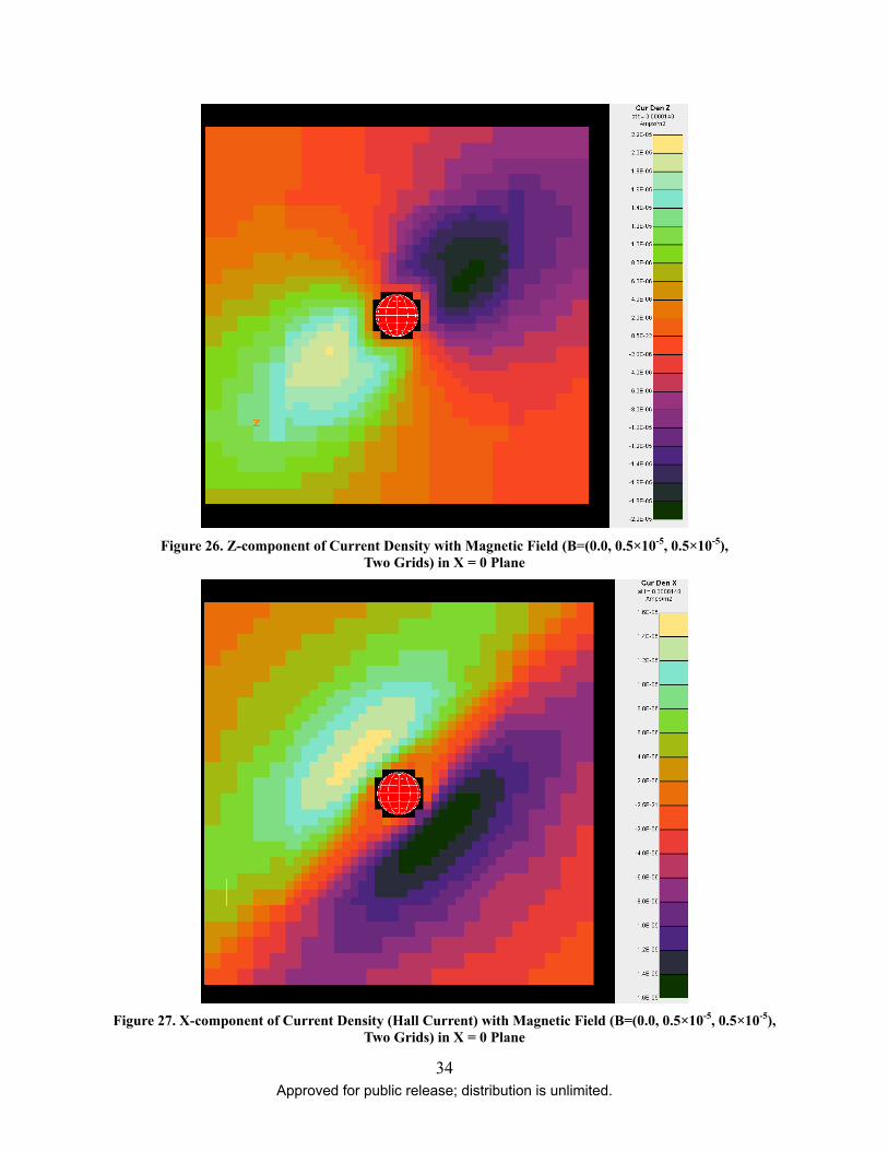
Figure 26. Z-component of Current Density with Magnetic Field (B=(0.0, 0.5×10-5, 0.5×10-5), Two Grids) in X = 0 Plane ...........................................................................................34

Figure 27. X-component of Current Density (Hall Current) with Magnetic Field (B=(0.0, 0.5×10-5, 0.5×10-5), Two Grids) in X = 0 Plane .............................................................................34

Figure 28. Calculated Currents Along the Z-axis for B=0 at t=14 µsec, Compared with Analytic Estimate Based on Calculated Potentials ........................................................................35

v Approved for public release; distribution is unlimited.

LIST OF TABLES

Page

Table 1. Impedance Results ...........................................................................................................14

Table 2. Parameters of Cubic Grids Used in Example Calculations ..............................................24

vi Approved for public release; distribution is unlimited.

T h i s p a g e i s i n t e n t i o n a l l y l e f t b l a n k .

1 Approved for public release; distribution is unlimited.

1. INTRODUCTION

In support of the larger goal to provide a plasma engineering capability to the spacecraft community, the objective of the Spacecraft Charging Modeling—Nascap-2k contract is to develop, incorporate, test, and validate new algorithms for the three-dimensional plasma-environment spacecraft interactions computational tool, Nascap-2k. Nascap-2k is being modified to extend the range of plasma physics phenomena that the code can simulate, make the advanced code capabilities more accessible to users, and improve and maintain both the graphical and non-graphical interfaces to the code. The upgraded code is being used to simulate problems of interest to AFRL, including support of the DSX (Demonstration and Science eXperiments) spacecraft and program.

1.1. First Year Progress

Details on progress during the period from September 19, 2011 through September 21, 2012 are given in the following sections. Key accomplishments are the following:

Prepared and sent Nascap-2k 4.1 Release to AFRL and NASA/MSFC for distribution.

Used Nascap-2k to model DSX.

Began functional and structural enhancements of Nascap-2k to be included in the next release.

Modified Nascap-2k to be able to specify and then optionally use a time-dependent tabular environment in a surface charging calculation.

Attended and made two presentations at the 12th Spacecraft Charging Technology Conference in Kitakyushu, Japan May 14 to 18, 2012.

Revised the implementation of a pseudopotential calculation technique to compute volume electron currents so that it now uses a finite element formalism. The magnetic field dependence of the currents was added.

Built and delivered a simple Java computer tool for the determination of the electron induced secondary yield material properties parameters that give the best fit to measured data.

1.1.1. Interoperability of Nascap-2k with Other Codes

The task to make Nascap-2k work well with other software includes four subtasks, two of which were addressed during the first year:

Improve ability to use a specified time-dependent tabular environment in a surface charging calculation.

Improve ability to run scripted jobs.


We implemented the ability to compute charging in a tenuous environment specified by a table of fluxes within energy bins and to perform Nascap-2k surface charging calculations using such a tabular environment. At the same time we implemented the ability to specify and use a tenuous environment described by a kappa distribution function.

We added the ability to specify that multiple environments be used successively within a single DoTimeSteps request.

We reviewed how Nascap-2k presently deals with quantities relevant to charging that change with time. We identified changes that would simplify the specification of time varying quantities. We also reviewed the script commands and identified several changes that would simplify the structure of the script.

As part of the effort to improve Nascap-2k’s handling of scripts, we revised Nascap-2k to eliminate the duplicate script handling coding in the Java GUI and N2kScriptRunner. Java GUI now calls a dynamically linked library (DLL) that includes all of the C++ code previously in N2kScriptRunner and in BEMDLL. N2kScriptRunner was modified to call the DLL in the same manner as the Java GUI. This change is already simplifying code maintenance.

1.1.2. Research Models of Spacecraft Charging and Discharging

We implemented the ability to display the dielectric stress (differential potential/thickness) on the Results and Results 3D tabs.

1.1.3. Maintenance and Support

Maintenance and support activities during this period included the following:

Release

Fixed bugs in Nascap-2k 4.1 Release Candidate and sent Nascap-2k 4.1 Release to AFRL and to NASA/MSFC for distribution.

Updated the documentation to reflect all of the code changes since the 4.1 Release.

As requested, sent source code for Nascap-2k 4.1 Release to Dr. Ira Katz at the Jet Propulsion Laboratory.

Developed a preliminary plan for multi-site development of Nascap-2k. This plan is included as Section 2.

As requested, sent Nascap-2k for LINUX and for Windows to Chris Roth of AER.

Software

Reviewed the source coding of Nascap-2k and discussed how the code design could be changed for ease of future development. We will make changes incrementally, with the goal of leaving the code more transparent each time a change is made.

Transferred Nascap-2k source code to a Windows 7 computer with an i7 processor. This computer will be used to refine the multiprocessing and 64-bit capabilities of the code. As


part of this effort, the C++ code was modified to use the msxml 6 xml interpretation package rather than the msxml 3 package previously used.

Revised the Nascap-2k C++ and Fortran coding to incorporate all of the science coding into a single dynamically loaded library (DLL). The static Fortran and C libraries are maintained as before. The change reduces duplicative code, eliminates the need for dynamic loading and unloading of libraries under LINUX, simplifies the overall code structure, and further isolates coding that handles the interactions between components.

Switched from using Java 6 to Java 7. Added coding to reduce the frequency that the three-dimensional display disappears due to an incompatibility of the latest version of Java3D and Java 7.

Explored Scene Graph software packages for an alternative to Java3D for the three dimensional display of Nascap-2k. No adequate alternatives were identified.

Updated the LINUX/MACOS X version of Nascap-2k. This was primarily updating the Makefiles to reflect the reorganized code.

User Support

Provided assistance with low potential charging calculations, including C/NOFS, to Dale Ferguson and David Cooke of AFRL.

Provided assistance with adapting the DMSP Object ToolKit model to Dale Ferguson of AFRL.

Determined why Dale Ferguson obtained unphysical results when using Nascap-2k to model the floating potential of a high power LEO spacecraft. Made recommendations regarding code changes.

Science

Built and delivered a simple Java computer tool that can be used to determine the electron induced secondary yield material properties parameters that give the best fit to measured data. Further discussion appears in Section 5.

Provided information on the 2004-2005 analysis of how low level charging of DMSP would impact the SSULI optical instrument. We participated in a teleconference on recent anomalous noise in the same instrument (modified to eliminate the noise source previously identified) that may also be due to spacecraft charging.

Made a number of small improvements to Nascap-2k’s wake handling capabilities.

Completed, implemented, and tested a new formulation of charge stabilization for Hybrid PIC calculations that properly handles sheath edges in large volume elements and wakes. The documentation was revised to reflect these changes. Further discussion appears in Section 6.

1.1.4. Apply Nascap-2k to DSX

We prepared an updated DSX Road Map. This is included as Section 3.


We computed the impedance of the DSX system from Nascap-2k calculations for 2, 10, and 12 kHz at 1 kV in vacuum and in a plasma. The approach and results for these initial calculations are in Section 4.

We validated the pseudopotential method for the computation of electron currents throughout space by comparison with analytic calculations. The results are included in the paper presented at the 12th Spacecraft Charging Technology Conference.

We revised the implementation of volume electron currents so that it now uses a finite element formalism. In this approach there is a clear recipe for getting the currents and matrix elements, instead of the face currents and edge currents used previously.

We added the magnetic field dependence of the electron currents.

Further discussion appears in Section 7.

1.1.5. Advanced EHF Analysis

We began an analysis of how each environment sensor of the AFRL sensor tower will respond to the various environments. We gathered and reviewed the available information on the Advanced EHF spacecraft and the AFRL instrument tower. We compiled descriptions of the instruments that are sensitive to the plasma environment.

We built Object ToolKit models of the Advanced EHF spacecraft and the AFRL instrument tower. The tower model is a low resolution model for preliminary calculations. We performed preliminary calculations.

Preliminary calculations showed that, if the spacecraft geometry and fraction of the surface that is conducting is properly represented by the spacecraft model, chassis charging will be rare in sunlight.

The determination of the influence of the Langmuir probes and the spacecraft structure on the RPA and flux probe measurements will require reverse trajectory calculations.

1.1.6. Nascap-2k Enhancements Funded by Other Organizations

Other organizations support SAIC to do Nascap-2k development needed for modeling their spacecraft. The following recent improvements were supported by the Jet Propulsion Laboratory.

Revised treatment of charging in the presence of high v×B potentials so that differential charging in a time varying environment would be handled correctly.

Extended the Solar Wind and Auroral analytic ion flux models to Mach numbers over 20.

Implemented import of a NX I-DEAS TMG VUFF file into Object ToolKit.

Implemented export of object surface information to a Tecplot data file.


1.2. Reports and Meetings

Dr. Victoria A. Davis and Dr. Myron J. Mandell traveled to Kirtland AFB for a contract kickoff meeting. We made three presentations:

1. Contract kickoff management presentation 2. Seminar on Nascap-2k 3. Seminar on progress with DSX calculations since our November 2009 briefing at

Hanscom AFB and where we plan to go next. (This seminar consisted almost entirely of work performed under previous contracts.)

Dr. Victoria A. Davis and Dr. Myron J. Mandell traveled to AFRL/VSBX at Kirtland AFB for a contract review on August 28. We made three presentations on progress to date:

1. Contract review 2. DSX analysis progress 3. Advanced EHF analysis progress

Dr. Victoria A. Davis attended the 12th Spacecraft Charging Technology Conference in Kitakyushu, Japan May 14 to 18, 2012. She presented two papers:

1. Comparison of low Earth orbit wake current collection simulations using SPIS, MUSCAT, and Nascap-2k computer codes, V.A. Davis, M.J. Mandell, (Science Applications International Corporation), D.C. Cooke, A. Wheelock, (U.S. Air Force Research Laboratory), J.-C. Matéo-Vélez, J.-F. Roussel (ONERA), D. Payan (CNES), M. Cho (Kyushu Institute of Technology), K. Koga (Japan Aerospace Exploration Agency)

2. Pseudopotential Algorithms for Simulation of Current Flow on and about a VLF Plasma Antenna, M.J. Mandell, V.A. Davis, (Science Applications International Corporation), D.L. Cooke, A.T. Wheelock, (Air Force Research Laboratory)

The code comparison study was presented orally and the psuedopotential paper was presented as a poster. The code comparison paper was submitted for publication in a special issue of IEEE Transactions on Plasma Science.

All presentations are included in the quarterly report for the relevant period.

1.3. Scientific Reports and Journal Articles

The following publications were supported in total or in part by this contract.

Nascap-2k Self-Consistent Simulations of a VLF Plasma Antenna, V. A. Davis, M. J. Mandell, D. L. Cooke, A. T. Wheelock, and C. J. Roth, IEEE Trans Plasma Science, 40, p. 1239, 2012.


1.4. Personnel

The project staffing remains as specified in the proposal. Dr. Victoria A. Davis is the project manager and Dr. Myron J. Mandell is the principal investigator. The following SAIC staff members have contributed to the work reported here.

Dr. Victoria A. Davis

Dr. Myron J. Mandell

Dr. Robert A. Kuharski

Ms. Barbara M. Gardner

Dr. Michael Brown-Hayes


2. MULTISITE DEVELOPMENT PLAN

The following outlines the key aspects of the proposed multisite development plan.

Historical approach to maintaining Nascap-2k integrity

Tight control of releases and source code

Close working relationships between programmers

With multisite development, coding standards more important

Programmer’s documentation

Written programming standards

Documented test procedures

Central repository still needed for source control, testing, and release (including documentation)

Important that all sites

Follow standards

Test that existing functionality is maintained

Provide revisions to affected documentation


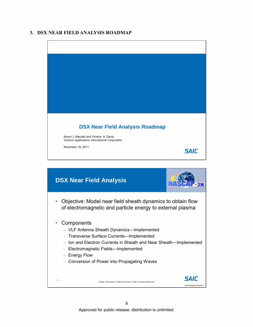
3. DSX NEAR FIELD ANALYSIS ROADMAP

Myron J. Mandell and Victoria A. Davis, Science Applications International Corporation

November 18, 2011

DSX Near Field Analysis Roadmap

Energy | Environment | National Security | Health | Critical Infrastructure2

SAIC Roadmap Nov2011

DSX Near Field Analysis

• Objective: Model near field sheath dynamics to obtain flow of electromagnetic and particle energy to external plasma

• Components– VLF Antenna Sheath Dynamics—Implemented– Transverse Surface Currents—Implemented– Ion and Electron Currents in Sheath and Near Sheath—Implemented– Electromagnetic Fields—Implemented – Energy Flow– Conversion of Power into Propagating Waves




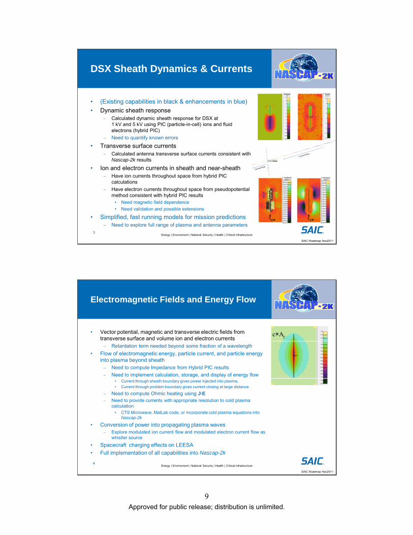
DSX Sheath Dynamics & Currents

• (Existing capabilities in black & enhancements in blue)• Dynamic sheath response

– Calculated dynamic sheath response for DSX at 1 kV and 5 kV using PIC (particle-in-cell) ions and fluid electrons (hybrid PIC)

– Need to quantify known errors

• Transverse surface currents– Calculated antenna transverse surface currents consistent with

Nascap-2k results

• Ion and electron currents in sheath and near-sheath– Have ion currents throughout space from hybrid PIC

calculations – Have electron currents throughout space from pseudopotential

method consistent with hybrid PIC results• Need magnetic field dependence• Need validation and possible extensions

• Simplified, fast running models for mission predictions– Need to explore full range of plasma and antenna parameters

x

y

x

y



Electromagnetic Fields and Energy Flow

• Vector potential, magnetic and transverse electric fields from transverse surface and volume ion and electron currents

– Retardation term needed beyond some fraction of a wavelength• Flow of electromagnetic energy, particle current, and particle energy

into plasma beyond sheath– Need to compute Impedance from Hybrid PIC results– Need to implement calculation, storage, and display of energy flow

• Current through sheath boundary gives power injected into plasma.• Current through problem boundary gives current closing at large distance

– Need to compute Ohmic heating using J·E– Need to provide currents with appropriate resolution to cold plasma

calculation• CTS Microwave, MatLab code, or incorporate cold plasma equations into

Nascap-2k

• Conversion of power into propagating plasma waves– Explore modulated ion current flow and modulated electron current flow as

whistler source• Spacecraft charging effects on LEESA• Full implementation of all capabilities into Nascap-2k

c×Ay




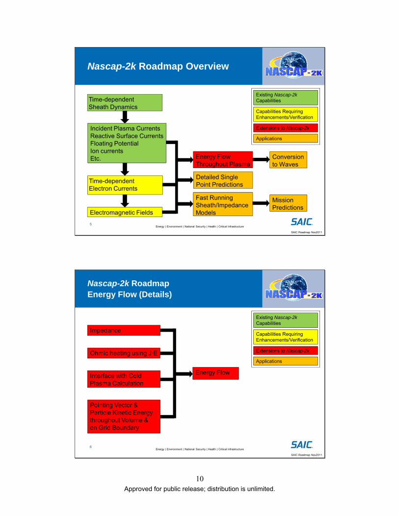
Nascap-2k Roadmap Overview

Time-dependent Sheath Dynamics

Time-dependent Electron Currents

Incident Plasma CurrentsReactive Surface CurrentsFloating PotentialIon currentsEtc.

Electromagnetic Fields

Fast Running Sheath/Impedance Models

Energy Flow Throughout Plasma

Existing Nascap-2k Capabilities

Capabilities Requiring Enhancements/Verification

Extensions to Nascap-2k

Applications

Conversion to Waves

Detailed Single Point Predictions

Mission Predictions



Nascap-2k Roadmap Energy Flow (Details)

Impedance

Interface with Cold Plasma Calculation

Ohmic heating using J·E

Energy Flow

Existing Nascap-2k Capabilities

Capabilities Requiring Enhancements/Verification

Extensions to Nascap-2k

Applications

Pointing Vector & Particle Kinetic Energy throughout Volume & on Grid Boundary


4. DSX ANTENNA IMPEDANCE FROM NASCAP-2K CALCULATIONS—FIRST ESTIMATE

Previously we simulated the DSX dipole antenna experiment. We computed the sheath structure and ion collection using a hybrid PIC approach with PIC ions and fluid barometric electron densities [1]. The plasma response, collected ion currents, and chassis floating potential were computed self-consistently with a 1 kV near-square-wave bias applied to the antenna elements. The near-square-wave bias was approximated by the first two components, as is planned during flight. The ion current density was computed during this calculation.

We used the results of these calculations to calculate the current flowing along the antenna elements, the electron current density throughout the surrounding volume, and the vector potential field [1]. One of the results of the pseudopotential algorithm used to compute the current flowing along each antenna element is the injected current. This is the current that must be supplied by the power supply in order for the antenna surface potentials to be as specified, i.e., the total change in charge on the antenna element divided by the timestep less the incident plasma current.

The Nascap-2k calculations to date assume that all surfaces are perfectly conductive and that the power supply is ideal. The system is primarily capacitive. Plasma interactions add a resistive component. Presently, inductive and magnetic field effects are ignored. The inductive and magnetic field effects remain to be quantified. It remains to be verified that, on the length scale of the calculations, the only significant magnetic field effect is the effect of the ambient field on the electron current flow.

The radius of the antenna booms in the Nascap-2k model of the spacecraft, 5 cm, was set so that their capacitance to space is the same as the actual wire frame booms. The capacitance of a single 5 inch diameter antenna element (slightly larger than in the model) to infinity was calculated to be 364 pF. The capacitance of an antenna element 1 m above a ground plane was calculated to be 681 pF, and for 3 m above a ground plane, 510 pF. These values can be compared with the August 2009 measurement of “800+ pF” for the capacitance of a single boom in the ATK facility. The boom was suspended 1 m above the floor and 3 m below the ceiling. A simple Nascap-2k model was used to determine that the total capacitance between two oppositely biased antenna elements is 213 pF.

We used the previously computed injected currents and the applied potential bias to compute the impedance of the antenna.

4.1. Equations and Integrals

If we use the symbols V, for the applied antenna voltage, I, for the injected current, R, for the radiation resistance, and X, for the reactance, by definition we have,

tjexpIjXRtjexpV . (1)

We can then use trigonometric identities to obtain


cos

I

VR

, sin

I

VX

, and

22 XRI

V

(2)

The reactance consists of the capacitance C and inductance L, C

1LX

. As we are

presently ignoring the inductive contribution, this gives a relationship between the capacitance (which is nearly independent of frequency) and the reactance.

In the Nascap-2k calculations to date, the applied differential voltage is

t3sinVtsinVV 1oapplied

, (3)

where 3VV,volts24.1273V o1o , and f2 , where f = 10 kHz, 12 kHz, or 2 kHz. Thus

V = 636.662 volts.

To compute the magnitude and phase of each component of the injected current, we use linearity and the identities

oo

T

0o1o cos

2

Idttsint3sinItsinI

T

1

and (4)

o1

T

0o1o cos

2

Idtt3sint3sinItsinI

T

1

. (5)

For this system, as we are assuming the system is purely capacitive and 3VV o1 , the

capacitance is independent of frequency and 1o II .

We compute the integrals

T

0oinjected dttsintI

T

1 (6)

and

T

0oinjected dtt3sintI

T

1

(7)

for a few cycles and select the value of δo that maximizes the integrals. We use δo, the average of the computed values of Io and I1, and Equations (2) to compute the impedance.

We also have that the average power is given by 2cosIV .


4.2. Vacuum Solution

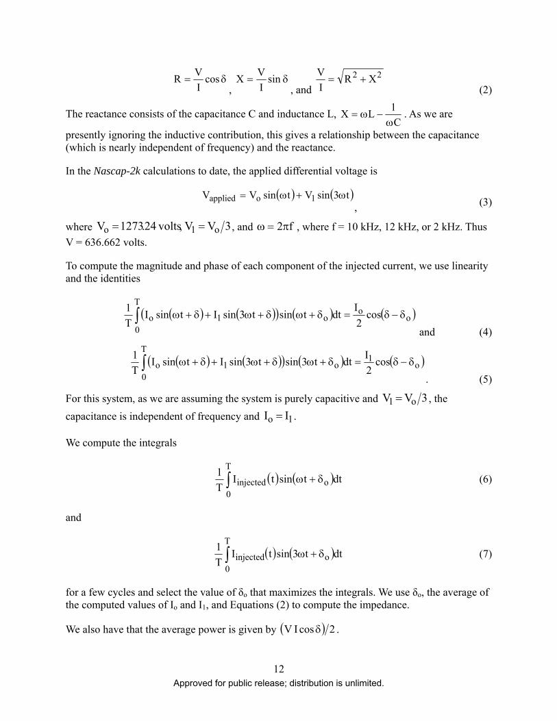
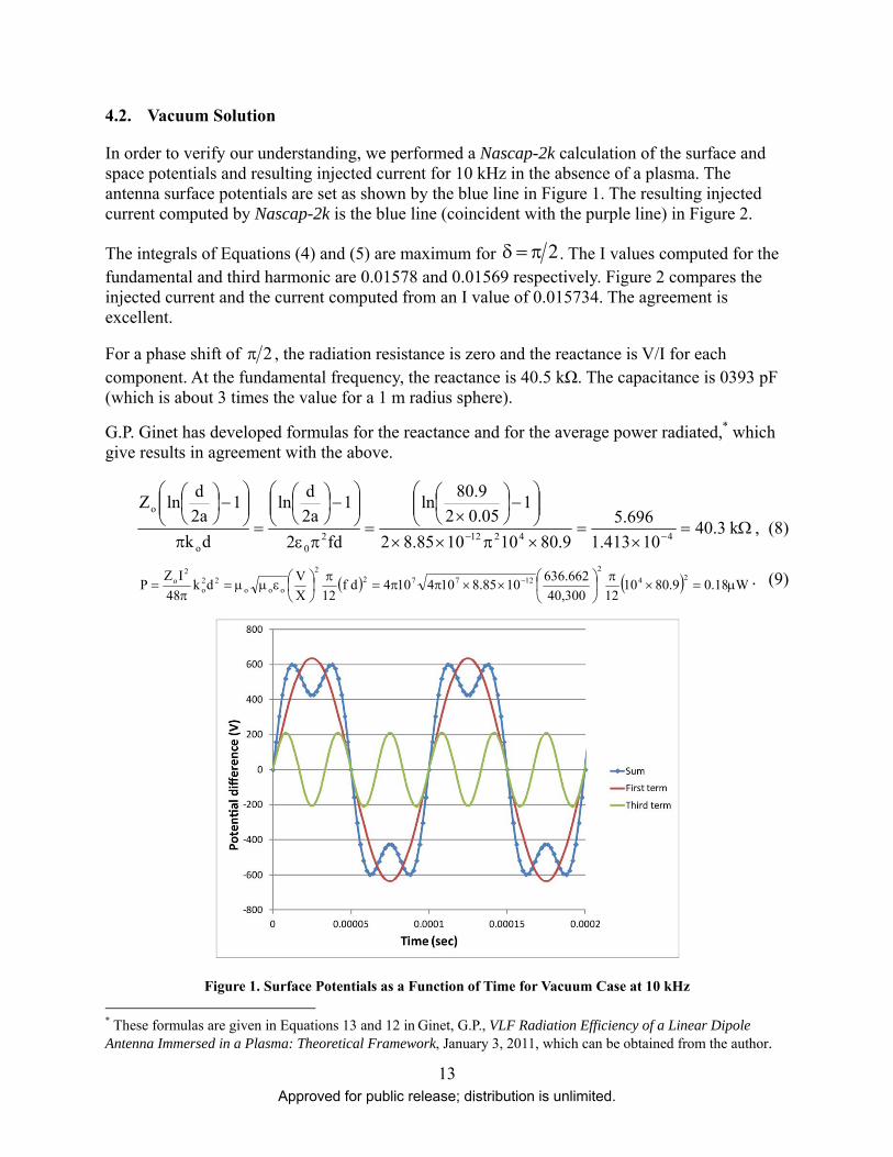
In order to verify our understanding, we performed a Nascap-2k calculation of the surface and space potentials and resulting injected current for 10 kHz in the absence of a plasma. The antenna surface potentials are set as shown by the blue line in Figure 1. The resulting injected current computed by Nascap-2k is the blue line (coincident with the purple line) in Figure 2.

The integrals of Equations (4) and (5) are maximum for 2 . The I values computed for the fundamental and third harmonic are 0.01578 and 0.01569 respectively. Figure 2 compares the injected current and the current computed from an I value of 0.015734. The agreement is excellent.

For a phase shift of 2 , the radiation resistance is zero and the reactance is V/I for each component. At the fundamental frequency, the reactance is 40.5 kΩ. The capacitance is 0393 pF (which is about 3 times the value for a 1 m radius sphere).

G.P. Ginet has developed formulas for the reactance and for the average power radiated,* which give results in agreement with the above.

k3.4010413.1

696.5

9.80101085.82

105.02

9.80ln

fd2

1a2

dln

dk

1a2

dlnZ

4421220o

o

, (8)

W18.09.80101240,300

636.6621085.8104104df

12X

Vdk

48

IZP

24

2

127722

ooo22

o

2o

. (9)

Figure 1. Surface Potentials as a Function of Time for Vacuum Case at 10 kHz

* These formulas are given in Equations 13 and 12 in Ginet, G.P., VLF Radiation Efficiency of a Linear Dipole Antenna Immersed in a Plasma: Theoretical Framework, January 3, 2011, which can be obtained from the author.


Figure 2. Injected Current Computed from Potentials in Figure 1 Compared with the Injected Current Computed from the Integral

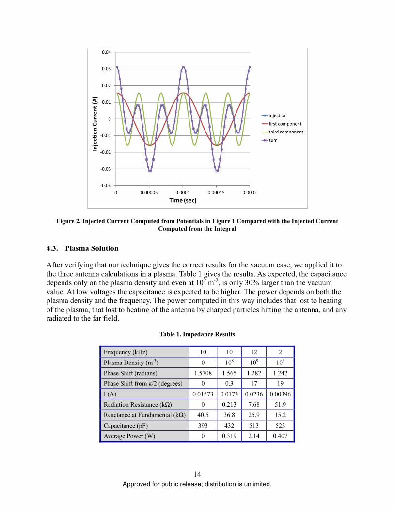
4.3. Plasma Solution

After verifying that our technique gives the correct results for the vacuum case, we applied it to the three antenna calculations in a plasma. Table 1 gives the results. As expected, the capacitance depends only on the plasma density and even at 109 m-3, is only 30% larger than the vacuum value. At low voltages the capacitance is expected to be higher. The power depends on both the plasma density and the frequency. The power computed in this way includes that lost to heating of the plasma, that lost to heating of the antenna by charged particles hitting the antenna, and any radiated to the far field.

Table 1. Impedance Results

Frequency (kHz) 10 10 12 2

Plasma Density (m-3) 0 108 109 109

Phase Shift (radians) 1.5708 1.565 1.282 1.242

Phase Shift from π/2 (degrees) 0 0.3 17 19

I (A) 0.01573 0.0173 0.0236 0.00396

Radiation Resistance (kΩ) 0 0.213 7.68 51.9

Reactance at Fundamental (kΩ) 40.5 36.8 25.9 15.2

Capacitance (pF) 393 432 513 523

Average Power (W) 0 0.319 2.14 0.407


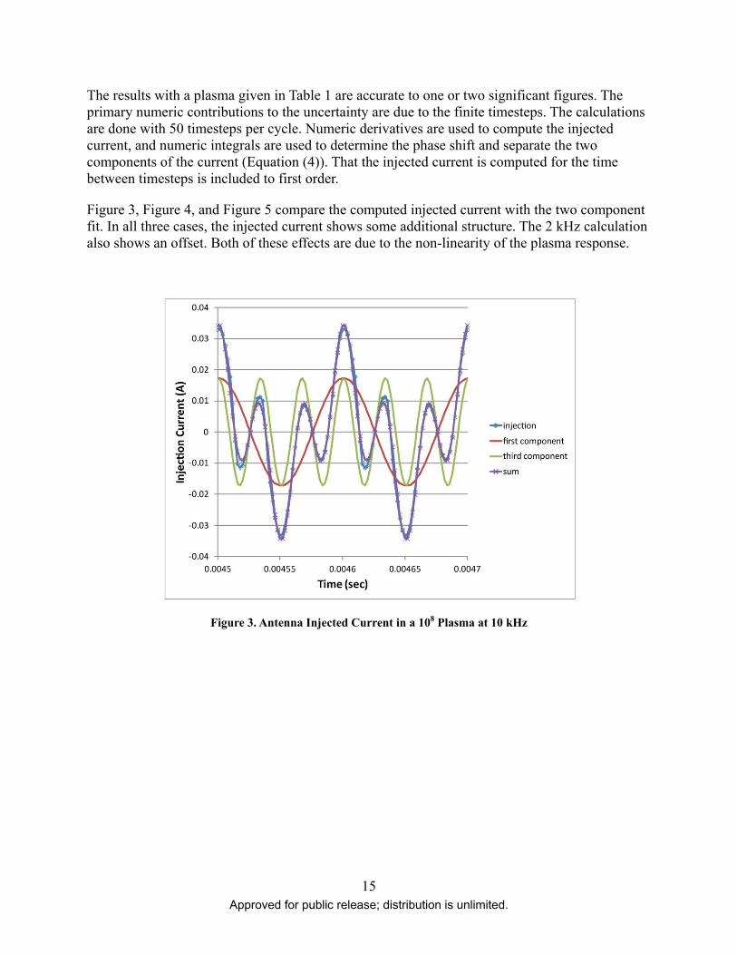
The results with a plasma given in Table 1 are accurate to one or two significant figures. The primary numeric contributions to the uncertainty are due to the finite timesteps. The calculations are done with 50 timesteps per cycle. Numeric derivatives are used to compute the injected current, and numeric integrals are used to determine the phase shift and separate the two components of the current (Equation (4)). That the injected current is computed for the time between timesteps is included to first order.

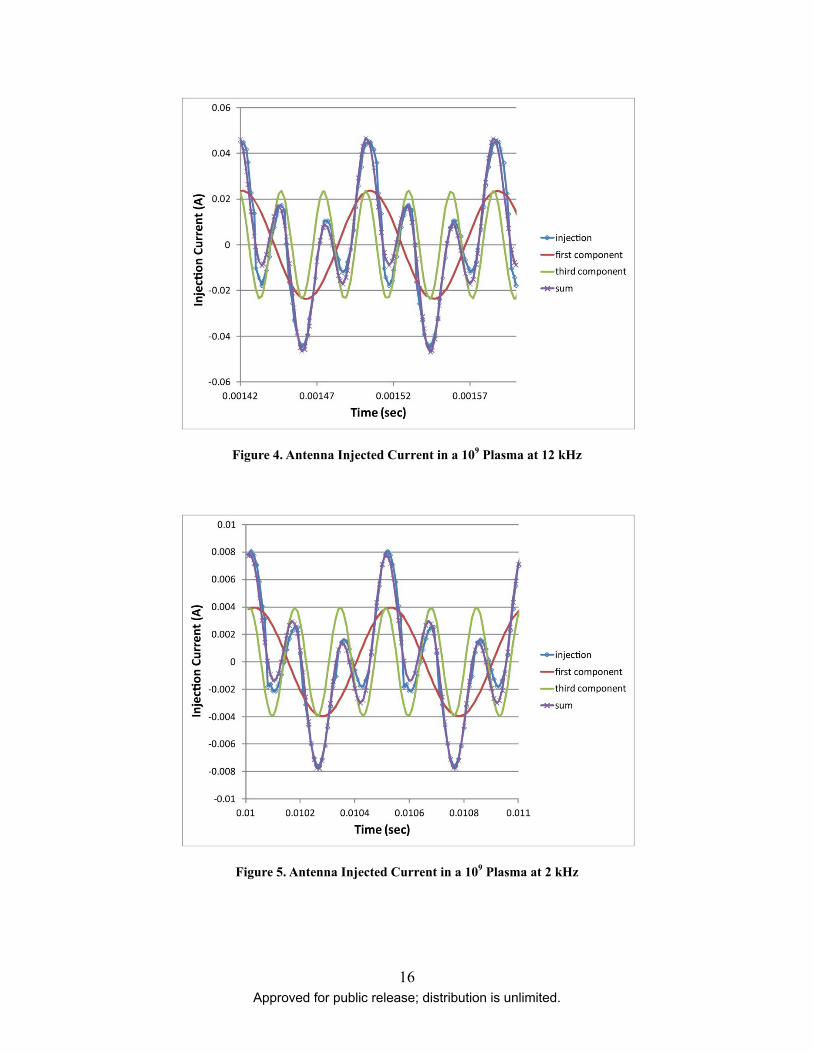
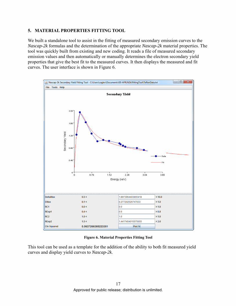
Figure 3, Figure 4, and Figure 5 compare the computed injected current with the two component fit. In all three cases, the injected current shows some additional structure. The 2 kHz calculation also shows an offset. Both of these effects are due to the non-linearity of the plasma response.

Figure 3. Antenna Injected Current in a 108 Plasma at 10 kHz





5. MATERIAL PROPERTIES FITTING TOOL

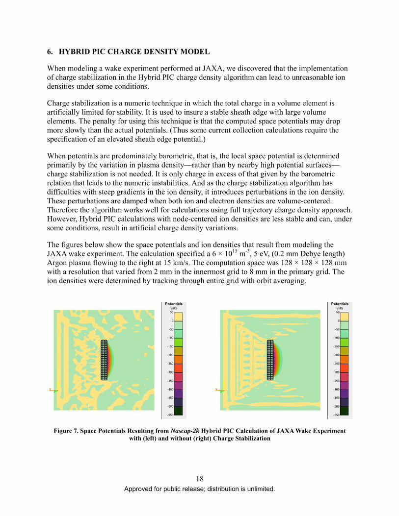
We built a standalone tool to assist in the fitting of measured secondary emission curves to the Nascap-2k formulas and the determination of the appropriate Nascap-2k material properties. The tool was quickly built from existing and new coding. It reads a file of measured secondary emission values and then automatically or manually determines the electron secondary yield properties that give the best fit to the measured curves. It then displays the measured and fit curves. The user interface is shown in Figure 6.

Figure 6. Material Properties Fitting Tool

This tool can be used as a template for the addition of the ability to both fit measured yield curves and display yield curves to Nascap-2k.


6. HYBRID PIC CHARGE DENSITY MODEL

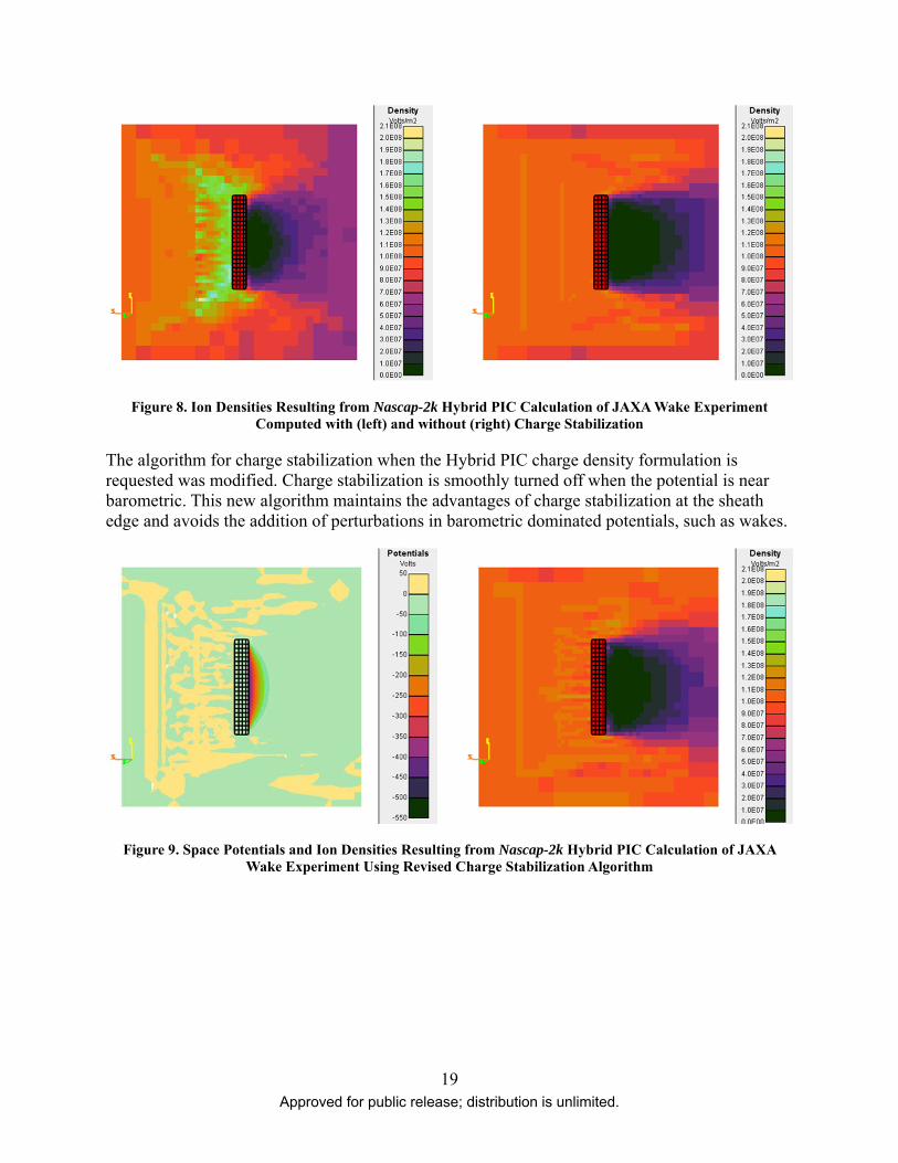
When modeling a wake experiment performed at JAXA, we discovered that the implementation of charge stabilization in the Hybrid PIC charge density algorithm can lead to unreasonable ion densities under some conditions.

Charge stabilization is a numeric technique in which the total charge in a volume element is artificially limited for stability. It is used to insure a stable sheath edge with large volume elements. The penalty for using this technique is that the computed space potentials may drop more slowly than the actual potentials. (Thus some current collection calculations require the specification of an elevated sheath edge potential.)

When potentials are predominately barometric, that is, the local space potential is determined primarily by the variation in plasma density—rather than by nearby high potential surfaces— charge stabilization is not needed. It is only charge in excess of that given by the barometric relation that leads to the numeric instabilities. And as the charge stabilization algorithm has difficulties with steep gradients in the ion density, it introduces perturbations in the ion density. These perturbations are damped when both ion and electron densities are volume-centered. Therefore the algorithm works well for calculations using full trajectory charge density approach. However, Hybrid PIC calculations with node-centered ion densities are less stable and can, under some conditions, result in artificial charge density variations.

The figures below show the space potentials and ion densities that result from modeling the JAXA wake experiment. The calculation specified a 6 × 1015 m-3, 5 eV, (0.2 mm Debye length) Argon plasma flowing to the right at 15 km/s. The computation space was 128 × 128 × 128 mm with a resolution that varied from 2 mm in the innermost grid to 8 mm in the primary grid. The ion densities were determined by tracking through entire grid with orbit averaging.

Figure 7. Space Potentials Resulting from Nascap-2k Hybrid PIC Calculation of JAXA Wake Experiment with (left) and without (right) Charge Stabilization


Figure 8. Ion Densities Resulting from Nascap-2k Hybrid PIC Calculation of JAXA Wake Experiment Computed with (left) and without (right) Charge Stabilization

The algorithm for charge stabilization when the Hybrid PIC charge density formulation is requested was modified. Charge stabilization is smoothly turned off when the potential is near barometric. This new algorithm maintains the advantages of charge stabilization at the sheath edge and avoids the addition of perturbations in barometric dominated potentials, such as wakes.

Figure 9. Space Potentials and Ion Densities Resulting from Nascap-2k Hybrid PIC Calculation of JAXA Wake Experiment Using Revised Charge Stabilization Algorithm


7. FINITE ELEMENT PSEUDOPOTENTIAL TREATMENT FOR NASCAP-2K ELECTRON CURRENTS

7.1. Introduction

It is desirable to have a non-PIC (particle-in-cell) method to calculate volume electron currents that satisfy the equation of continuity, other physical requirements, and are consistent with other Nascap-2k calculated quantities (e.g., Hybrid PIC). The method can be used to calculate electron currents within and near the sheath about a VLF antenna or other high-voltage object at frequencies that are low compared with both the electron plasma frequency, ωpe, and the electron cyclotron frequency, ωce. The currents can then be used to calculate electromagnetic radiation, ohmic heating, etc.

To satisfy this need, a pseudopotential approach to the computation of volume electron currents was developed. Local equilibrium electron densities are generated for each volume element as part of the Hybrid PIC ion dynamics simulation. Their time derivatives are the main drivers of volume electron currents. Space outside the calculation boundary can act as either a source or a sink for electrons, and object surfaces may act as electron sinks.

The electron current, jelec, must satisfy 0dt

dρelecelec j . To solve this we assume that jelec is

proportional to the gradient of a “pseudopotential,” ψ: σjelec , where the conductivity

tensor, σ, depends on the electron density and magnetic field. Note that the solution for the current is non-unique to the addition of any divergence-free current field. We assume that, provided appropriate boundary conditions are implemented, such circulating currents are not of concern to the problem being solved.

The main requirement for application of the pseudopotential approach to the calculation is that the electron density for each volume element (as used in the calculation of electrostatic potential during the Nascap-2k simulation) be stored (or computable) for each timestep. In addition, we need to establish boundary conditions at the external boundary and near the spacecraft and limit current flow to values the local electron population can support.

Nascap-2k provides the electron density, nelec, in each volume element as a function of time (usually as an analytic function of ion density and potential), and thereby the rate of change of

electron charge density, dt

dne

dt

d elecelec

, in each element.

7.2. Finite Element Formulation

The above equations can be combined as

dt

d elec σ . (10)

By standard finite element treatment, this equation is equivalent to minimizing the function


dt

d

2

1dV elecσ . (11)

Like the solution to Poisson’s equation, the integrals are calculated for each volume element. The pseudopotential is taken to be trilinear within each volume element, so it is given by

iii

e ψN)(ψ xx, (12)

where “i” are the nodes of the element indexed by “e”, and the Ni are the interpolants. Within each volume element, the integral is given by

i

eleci

3i

ij

jielec

3ji dt

dNdψ

dx

dN

dx

dNn,dψψ

2

1xx

xxBx (13)

As σ and ρelec are taken to be constant within each volume element, the integrals depend only on the volume size and shape. To minimize the volume integral in equation 2, we set its derivative with respect to ψ equal to zero. Thus the equation to be solved is

e

eleci

3

ejij dt

dNdA xx , (14)

with the finite element matrix for each element given by

x

N

x

Nn,dA

jielec

3eij Bx (15)

The 576 matrix elements of

x

N

x

Nd jix3 are precomputed for the unit cube. For each element,

the matrix elements are multiplied by the conductivity tensor and by the mesh size to obtain an 8×8 element matrix. Because the conductivity tensor is anisotropic for B≠0, matrix elements that are zero in the scalar case become nonzero in the presence of magnetic field.

The right hand side is formed by adding one-eighth of the charge density derivative (formed by differencing the current electron charge density with that at the previous timestep) for each volume element to each of its nodes after multiplying by the cube of the mesh size. The matrix elements are accumulated using a sparse matrix storage scheme for eventual solution using ICCG.


7.3. Boundary Conditions

7.3.1. Inner Boundary Conditions (Object Currents)

If an empty volume element neighbors a special element and has its electric field pointing away from the special element, then electrons are assumed to flow across the interface to the special element at the local plasma thermal current. Each of the four nodes on the corresponding face

has its right hand side augmented by a

electh

2

n

njx

4

1 , where jth is the electron plasma current in

the ambient plasma and na is the ambient plasma density. If the electric field points toward the special element, then no electron current crosses the interface, and no action is taken.

7.3.2. Outer Boundary Conditions

The pseudopotential is assumed to vary inversely with radius (measured from the grid center) outside the computational space. As a consequence, for each outer boundary square, each of its

nodes is assigned an additional diagonal matrix element given by

rrσr4

, where Ω is the

solid angle subtended by the outer boundary square relative to the grid center, r is the vector from the grid center, and σ is the conductivity tensor.

7.4. Grid Interface

Since the matrix elements for the entire computational grid are accumulated in order to use an ICCG solver, the matrix must be modified to place constraints on inner grid boundary nodes and assign matrix elements generated in the boundary volumes of the inner grid to outer grid nodes.

Presently, only the case of an inner grid surrounded by an outer grid with twice the mesh spacing is considered. Then each inner grid boundary node is of one of three types characterized by the number of outer grid nodes in its constraint:

Type 1 (coincident with an outer grid node), Type 2 (coincident with an outer grid edge center), or Type 4 (coincident with an outer grid face center).

After transferring the inner grid matrix elements to interact with the outer grid nodes as described below, each inner grid boundary node is constrained to have the average pseudopotential of its one, two, or four outer grid neighbors.

Type 1 nodes are processed first. For each type 1 node, its right hand side value is transferred to the coincident node. Then each interacting inner grid node is considered. If the interacting node is another (type 2 or type 4) boundary node, then the matrix element is doubled and applied between the coincident node and the next outer grid node beyond the interacting node (i.e., along the outer grid edge or outer grid face diagonal). If the interacting node is an inner grid interior node, the matrix element is applied between the interacting node and the coincident node.


Type 2 and then type 4 nodes are then processed. The right hand side value is divided evenly among the two or four outer grid neighbors. The remaining matrix elements between inner grid boundary nodes are discarded. Matrix elements with inner grid interior nodes are multiplied by one-half or one-fourth and applied between the interacting node and each of the two or four outer grid neighbors.

As each inner grid boundary node is processed, its equation is replaced by its constraint equation, meaning that any remaining matrix elements are discarded and then a matrix element is applied between the inner grid boundary node and each of its 1, 2, or 4 outer grid neighbors.

7.5. Conductivity Tensor

The conductivity tensor is taken to be the normal low frequency plasma conductivity tensor [2],

which, for B along the z-axis, is given by

2c

c

c

2c

0std

100

01

01

1σ . We take

m

ne2

0

and

4

1 pe

, so that

pe

cc

4

. Note that the off-diagonal terms (Hall terms) are

omitted when calculating the finite element solution for the pseudopotentials (as they do not contribute to the divergence of current), but included when calculating the actual currents from the pseudopotentials.

To obtain the conductivity matrix for arbitrary magnetic field requires the matrix multiplication

TσTσ stdT , where the transformation T is given by

coscossincossin

0cossin

sinsincoscoscos

T with

x

yz

B

Btan,

Bcos

B.

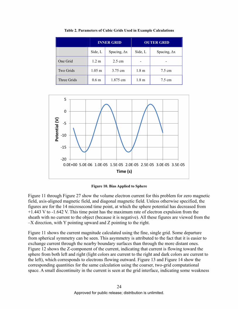
7.6. Example

As an example, we consider currents induced by a 10 cm radius sphere in a plasma with (nelec(0), Te)=(109 m-3, 1 eV). The calculations were done in one-grid, two-grid and three-grid configurations as detailed to Table 2. The sphere was sinusoidally biased at 70 kHz from -17 V to +3 V as shown in Figure 10. Potentials were calculated at each one microsecond timestep using Nascap-2k’s “Non-Linear” charge density formulation. The electron density for each volume

element was calculated using the potential, φ, at the element center using

0

01

/

eTe

a

elec

eT

n

n .

The rate of change of electron density at each time was determined by differencing with the previous time; otherwise values appropriate to the present time were used.


Table 2. Parameters of Cubic Grids Used in Example Calculations

INNER GRID OUTER GRID

Side, L Spacing, Δx Side, L Spacing, Δx

One Grid 1.2 m 2.5 cm - -

Two Grids 1.05 m 3.75 cm 1.8 m 7.5 cm

Three Grids 0.6 m 1.875 cm 1.8 m 7.5 cm

Figure 10. Bias Applied to Sphere

Figure 11 through Figure 27 show the volume electron current for this problem for zero magnetic field, axis-aligned magnetic field, and diagonal magnetic field. Unless otherwise specified, the figures are for the 14 microsecond time point, at which the sphere potential has decreased from +1.443 V to -1.642 V. This time point has the maximum rate of electron expulsion from the sheath with no current to the object (because it is negative). All these figures are viewed from the –X direction, with Y pointing upward and Z pointing to the right.

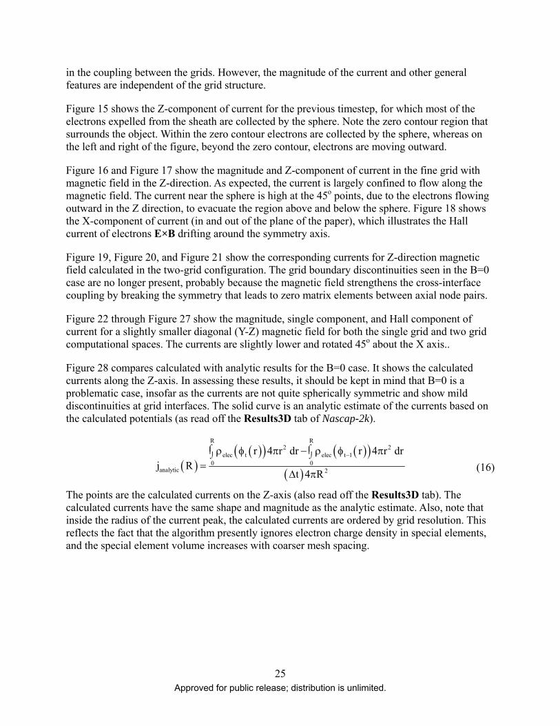
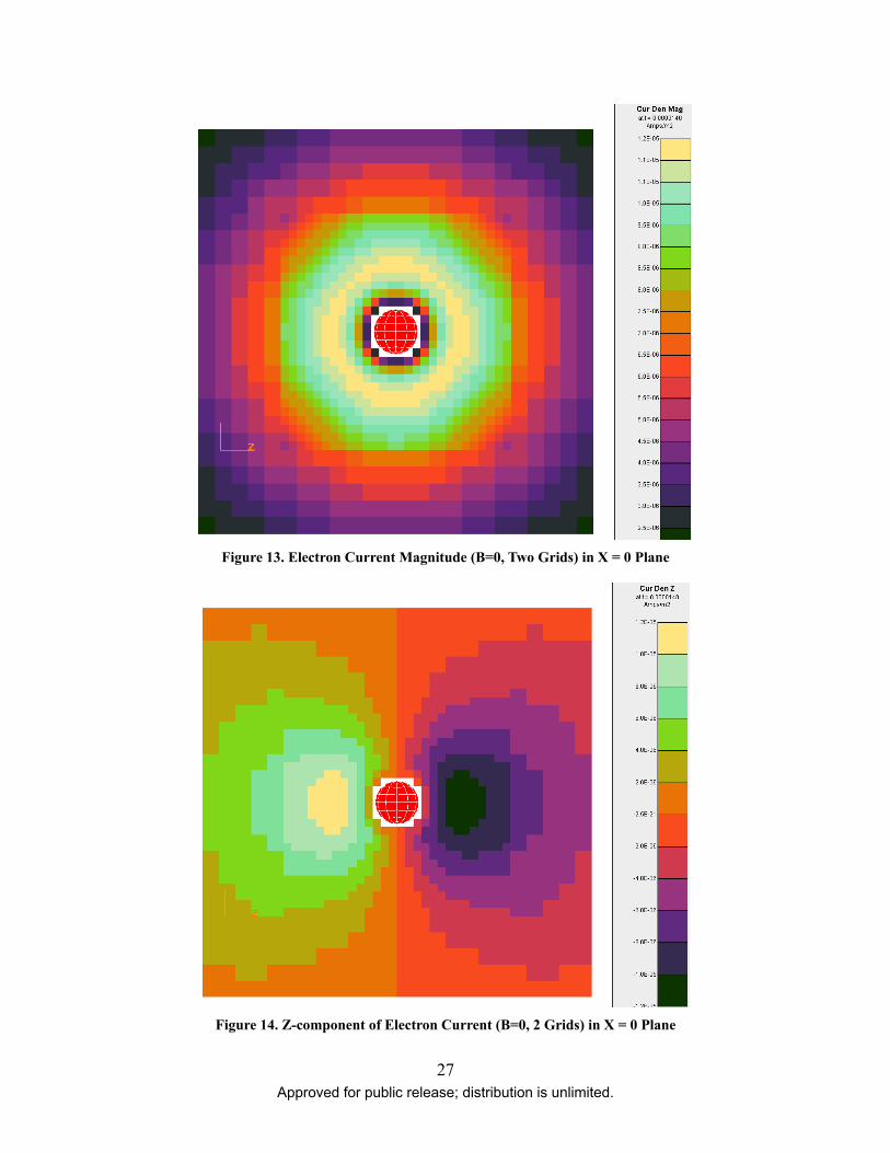
Figure 11 shows the current magnitude calculated using the fine, single grid. Some departure from spherical symmetry can be seen. This asymmetry is attributed to the fact that it is easier to exchange current through the nearby boundary surfaces than through the more distant ones. Figure 12 shows the Z-component of the current, indicating that current is flowing toward the sphere from both left and right (light colors are current to the right and dark colors are current to the left), which corresponds to electrons flowing outward. Figure 13 and Figure 14 show the corresponding quantities for the same calculation using the coarser, two-grid computational space. A small discontinuity in the current is seen at the grid interface, indicating some weakness

‐20

‐15

‐10

‐5

0

5

0.0E+00 5.0E‐06 1.0E‐05 1.5E‐05 2.0E‐05 2.5E‐05 3.0E‐05 3.5E‐05

Potential (V)

Time (s)


in the coupling between the grids. However, the magnitude of the current and other general features are independent of the grid structure.

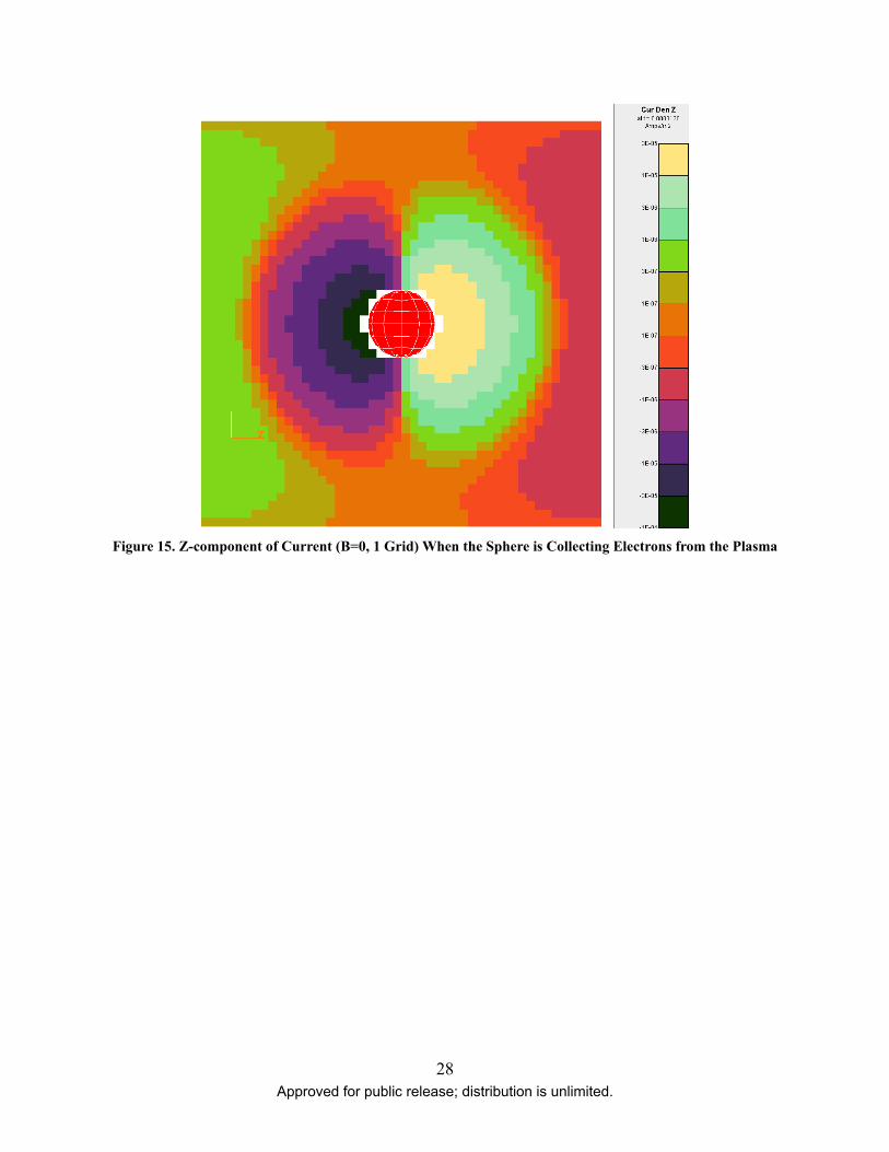
Figure 15 shows the Z-component of current for the previous timestep, for which most of the electrons expelled from the sheath are collected by the sphere. Note the zero contour region that surrounds the object. Within the zero contour electrons are collected by the sphere, whereas on the left and right of the figure, beyond the zero contour, electrons are moving outward.

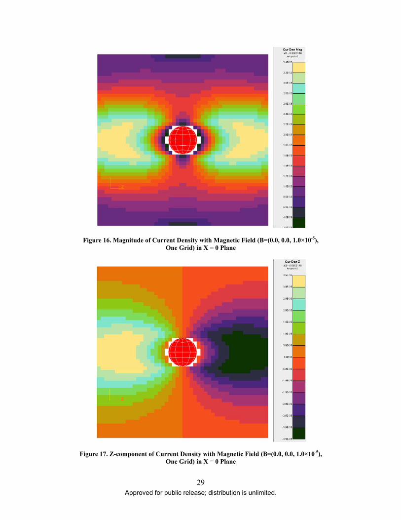
Figure 16 and Figure 17 show the magnitude and Z-component of current in the fine grid with magnetic field in the Z-direction. As expected, the current is largely confined to flow along the magnetic field. The current near the sphere is high at the 45o points, due to the electrons flowing outward in the Z direction, to evacuate the region above and below the sphere. Figure 18 shows the X-component of current (in and out of the plane of the paper), which illustrates the Hall current of electrons E×B drifting around the symmetry axis.

Figure 19, Figure 20, and Figure 21 show the corresponding currents for Z-direction magnetic field calculated in the two-grid configuration. The grid boundary discontinuities seen in the B=0 case are no longer present, probably because the magnetic field strengthens the cross-interface coupling by breaking the symmetry that leads to zero matrix elements between axial node pairs.

Figure 22 through Figure 27 show the magnitude, single component, and Hall component of current for a slightly smaller diagonal (Y-Z) magnetic field for both the single grid and two grid computational spaces. The currents are slightly lower and rotated 45o about the X axis..

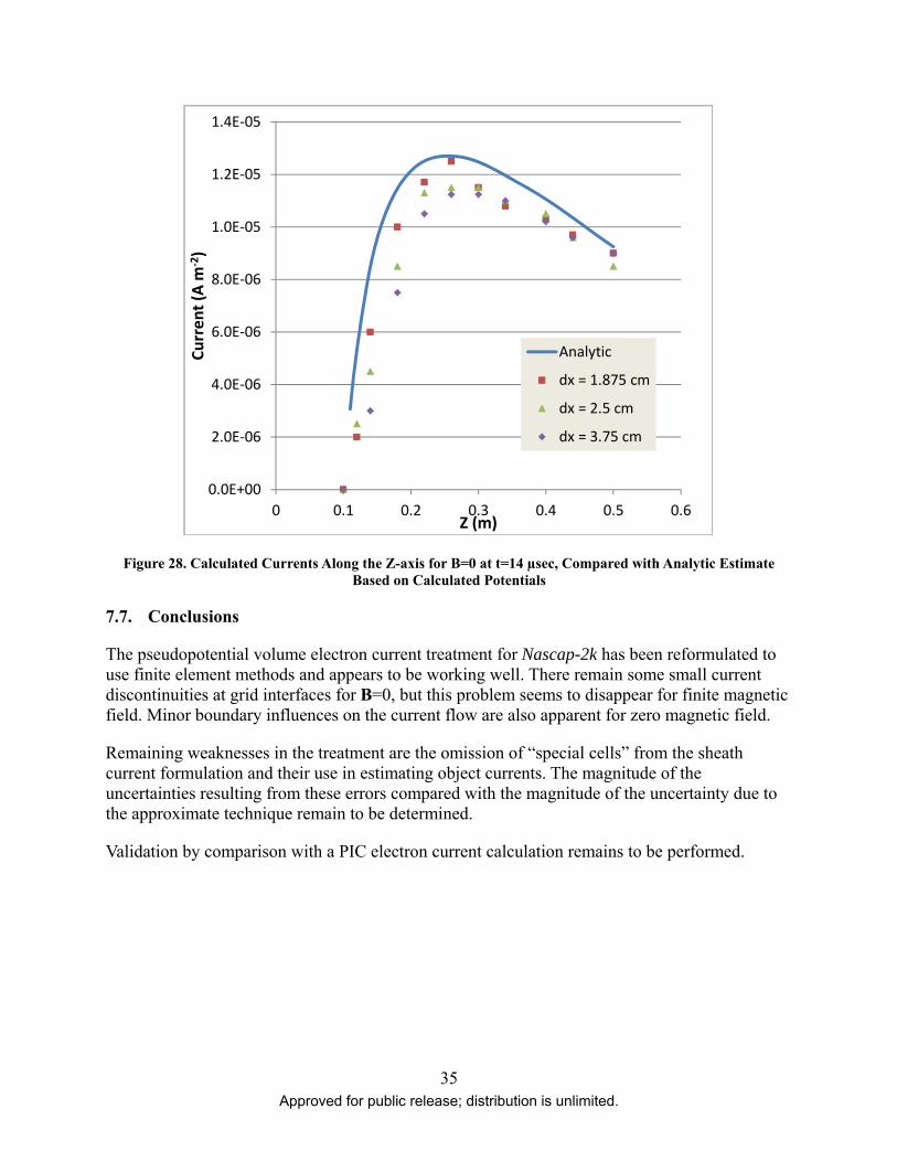
Figure 28 compares calculated with analytic results for the B=0 case. It shows the calculated currents along the Z-axis. In assessing these results, it should be kept in mind that B=0 is a problematic case, insofar as the currents are not quite spherically symmetric and show mild discontinuities at grid interfaces. The solid curve is an analytic estimate of the currents based on the calculated potentials (as read off the Results3D tab of Nascap-2k).

R R2 2

elec t elec t 10 0

analytic 2

r 4 r dr r 4 r drj R

t 4 R

(16)

The points are the calculated currents on the Z-axis (also read off the Results3D tab). The calculated currents have the same shape and magnitude as the analytic estimate. Also, note that inside the radius of the current peak, the calculated currents are ordered by grid resolution. This reflects the fact that the algorithm presently ignores electron charge density in special elements, and the special element volume increases with coarser mesh spacing.


Figure 11. Electron Current Magnitude (B=0, 1 Grid) in X = 0 Plane

Figure 12. Z-component of Electron Current (B=0, 1 Grid) in X = 0 Plane


Figure 13. Electron Current Magnitude (B=0, Two Grids) in X = 0 Plane

Figure 14. Z-component of Electron Current (B=0, 2 Grids) in X = 0 Plane


Figure 15. Z-component of Current (B=0, 1 Grid) When the Sphere is Collecting Electrons from the Plasma


Figure 16. Magnitude of Current Density with Magnetic Field (B=(0.0, 0.0, 1.0×10-5), One Grid) in X = 0 Plane

Figure 17. Z-component of Current Density with Magnetic Field (B=(0.0, 0.0, 1.0×10-5), One Grid) in X = 0 Plane


Figure 18. X-Component of Current Density (Hall Current) with Magnetic Field (B=(0.0, 0.0, 1.0×10-5), One Grid) in X = 0 Plane

Figure 19. Magnitude of Current Density with Magnetic Field (B=(0.0, 0.0, 1.0×10-5), Two Grids) in X = 0 Plane


Figure 20. Z-component of Current Density with Magnetic Field (B=(0.0, 0.0, 1.0×10-5), Two Grids) in X = 0 Plane

Figure 21. X-component of Current Density (Hall Current) with Magnetic Field (B=(0.0, 0.0, 1.0×10-5),

Two Grids) in X = 0 Plane


Figure 22. Magnitude of Current Density with Magnetic Field (B=(0.0, 0.5×10-5, 0.5×10-5), One Grid) in X = 0 Plane

Figure 23. Y-component of Current Density with Magnetic Field (B=(0.0, 0.5×10-5, 0.5×10-5), One Grid) in X = 0 Plane


Figure 24. X-Component of Current Density (Hall Current with Magnetic Field (B=(0.0, 0.5×10-5, 0.5×10-5),

One Grid) in X = 0 Plane

Figure 25. Magnitude of Current Density with Magnetic Field (B=(0.0, 0.5×10-5, 0.5×10-5), Two Grids) in X = 0 Plane


Figure 26. Z-component of Current Density with Magnetic Field (B=(0.0, 0.5×10-5, 0.5×10-5),


Figure 27. X-component of Current Density (Hall Current) with Magnetic Field (B=(0.0, 0.5×10-5, 0.5×10-5),



Figure 28. Calculated Currents Along the Z-axis for B=0 at t=14 µsec, Compared with Analytic Estimate Based on Calculated Potentials

7.7. Conclusions

The pseudopotential volume electron current treatment for Nascap-2k has been reformulated to use finite element methods and appears to be working well. There remain some small current discontinuities at grid interfaces for B=0, but this problem seems to disappear for finite magnetic field. Minor boundary influences on the current flow are also apparent for zero magnetic field.

Remaining weaknesses in the treatment are the omission of “special cells” from the sheath current formulation and their use in estimating object currents. The magnitude of the uncertainties resulting from these errors compared with the magnitude of the uncertainty due to the approximate technique remain to be determined.

Validation by comparison with a PIC electron current calculation remains to be performed.

0.0E+00

2.0E‐06

4.0E‐06

6.0E‐06

8.0E‐06

1.0E‐05

1.2E‐05

1.4E‐05

0 0.1 0.2 0.3 0.4 0.5 0.6

Current (A m

‐2)

Z (m)

Analytic

dx = 1.875 cm

dx = 2.5 cm

dx = 3.75 cm


REFERENCES [1] Davis, V.A., Mandell, M.J., Huston, S.L., Gardner, B.M., Plasma Interactions with

Spacecraft, Volume I, AFRL-RV-PS-TR-2011-0089, ADA542581, Science Applications International Corporation, San Diego, CA, April 2011.

[2] Kittel, C., Introduction to Solid State Physics, Third Edition, John Wiley and Sons, New York, NY, 1966, p. 242.

DISTRIBUTION LIST

DTIC/OCP 8725 John J. Kingman Rd, Suite 0944 Ft Belvoir, VA 22060-6218 1 cy AFRL/RVIL Kirtland AFB, NM 87117-5776 2 cys Official Record Copy AFRL/RVBXT/Adrian Wheelock 1 cy

37Approved for public release; distribution is unlimited.

This page is intentionally left blank.


Documents

SPACECRAFT CHARGING MODELING NASCAP- 2K · San Diego, CA 92121 . 21 September 2012 . ... Spacecraft Charging Modeling—Nascap-2k contract is to develop, ... Standard Form 298