Embed Size (px)
Citation preview

11111111111 ~1[lllllI11Ir~lrlllI111111111111~ 11111111111 3 1176 00504 3261
NASA-CR-167855 19820017934
NASA CR-167855 SSS-R-82-5249
ADDITIONAL EXTENSIONS TO THE NASCAP COMPUTER CODE,
Volume I
M.J. Mandell I. Katz
P.R. Stannard
S-CUBED
Prepared for
National Aeronautics and Space Administration
Lewis Research Center
Contract NAS3-2 2536
111111111111111111111111111111111111111111111 NF02683
https://ntrs.nasa.gov/search.jsp?R=19820017934 2018-09-06T19:51:42+00:00Z

1 Report No ~ I 2 Government AccessIon No 3 RecIpIent's Catalog No NASA CR-167855
4 T,tle and SubtItle 5 Report Date ADDITIONAL EXTENSIONS TO THE NASCAP COMPUTER CODE, October 1981 VOLUME I 6 PerformIng OrganIzatIon Code
7 Author(s) 8 PerformIng OrganIzatIon Report No
M. J. Mandell, I. Katz, P. R Stannard SSS-R-82-5249 10 Work Unot No
9 PerformIng OrganIzatIon Name and Address S-CUBED P. O. Box 1620 11 Contract or Grant No La Jolla, CA 92038 NAS3-22536
13 Type of Report and Perood Covered 12 Sponsorong Agency Name and Address Contractor Report
NatIonal AeronautIcs and Space AdmInIstratIon 9/9/1980 - 12/22/1981 LewIs Research Center 14 Sponsorong Agency Code 21000 Brookpark Road, Cleveland, OH 44135 5532
15 Supplementary Notes
ProJect Manager, James C. Roche, NASA-LewIs Research Center, Cleveland, OH
16 Abstract NASCAP IS a computer code that comprehenSIvely analyzes problems of spacecraft chargIng. USIng a fully three-dImensional approach, It can accurately predIct spacecraft potentIals under a varIety of condItIons. Under Contract No. NAS3-22536 several revIsIons and a few extensIons were Implemented with a vIew toward makIng NASCAP more powerful and easIer to use. Among the exten-sIons are a multIple electron/Ion gun test tank capabIlIty, and the abIlIty to model anIsotropIc and tIme-dependent space envIronments. These extensIons and revIsIons are documented In thIs volume.
Also documented here are a greatly extended MATCHG program and the prelImInary versIon of NASCAP/LEO. The InteractIve MATCHG code has been developed Into an extremely powerful tool for the study of materIal-envIronment interactIons. NASCAP/LEO, a three-dImensional code to study current collectIon under condItIons of hIgh voltages and short Oebye lengths, has been distrIbuted for prelImInary testIng.
There are two companIon volumes to thIs report. Volume II, NASA CR-167856. contaIns chapters entltl ed "ValIdatIon of the NASCAP Model USIng SatellIte Data". "NASCAP ApplIcatIons Guide". "DIfferentIal ChargIng of HIgh-Voltage Spacecraft· The EqUIlIbrium PotentIal of Insulated Sur-faces". and "Large Space Structure ModelIng". Volume III. NASA CR-167857. documents a computer code for the modelIng of plasmas external to Ion thrusters
17 Key Words ISuggested by Authorlsll 18 Dlstnbutlon Statement
NASCAP PublIcly avaIlable (no restrIctIons on Spacecraft Charging Plasma CollectIon provISIon to domestIc or foreIgn requesters) Computer SImulatIon
19 Securoty Oasslf (of th,s report)
1
20 Securoty Classlf (of thIs pagel 121
No of Pages 122 Proce-UNCLASSI FlED UNCLASSI FlED 250
• For sale by the National Technical Information SerVice, Springfield Vlrgl~la 22161
NASA·C·168 (Rev 10.75)

Chapter
l.
2.
3.
TABLE OF CONTENTS
SUMMARY ••••
INTRODUCTION
. . . . . . . . . . . . . . .
NASCAP/GEO REVISIONS
2.1 CONVERSION TO ASCII FORTRAN •••
2.2 NASCAP POCKET GUIDE •••••
2.3
2.2.1 2.2.2
NASCAP Pocket Guide Errata and Updates
OPTION REVISIONS • • • • • • •
Page
1
3
5
5
8
8 15
17
2.3.1 Justifications for New Options 17
2.3.1.1 Flux Definition. • • 19 2.3.1.2 Options Not Documented • 19
2.3.2 Description of New Options
2.4 OUTPUT REVISIONS ••••
2.5 SECONDARY ELECTRON REVIEW
2.5.1 A Reformulation of Secondary
19
26
28
Electron Emission. • • • • • • •• 28 2.5.2 Fitting of Four Parameter Form to
Stopping Power Data • • • • . • •• 32 2.5.3 Ion-Induced Secondary Electron
Emission • • •• 42
NASCAP/GEO EXTENSIONS • •
3.1 OBJDEF EXTENSION
3.2 NEW DISCHARGE CAPABILITY
3.2.1 General Principles Governing
44
44
44
Discharges •.••.•••• 44 3.2.2 Charge Redistribution - Specific
Cases .•.••.•••.•••• 48
i

TABLE OF CONTENTS (Continued)
Chaeter Page
3.3 MULTIPLE TEST TANK ENVIRONMENT · · · · 51
3.3.1 Theory . . . . · · · · 51 3.3.2 Implementation · · · · · 58
3.3.2.1 General Considerations 58 3.3.2.2 Usage · · · · · · · · 59 3.3.2.3 Gun Definition Input
Speci fication 60 3.3.2.4 Examples. 62
3.3.3 Cylindrical Tank · · · · · · · . . 66
3.4 SPACE ENVIRONMENT • 69
3.4.1 Anisotropic Flux · · · · 69
3.4.1.1 The Coordinate System 70 3.4.1.2 Angular Distribution
Function • · · · · · · 72 3.4.1.3 Current Collection. 73 3.4.1.4 Fitting Data • 77
3.4.2 DIRECT and UPDATE • · · · 83
3.4.2.1 DIRECT • · · · · · · · 83 3.4.2.2 Anisotropic 86 3.4.2.3 UPDATE • · · 87 3.4.2.4 Summary · · 89
3.4.3 Format for Tabulated Spectral Data · · · · . · · · · · 90
4. PLOTTING EXTENSIONS - NASCAP*PLOTREAD • · 94
5. NASCAP*MATCHG • · · · · · · · · · · · · · 100
5.1 PROGRAM STRUCTURE • · · · · · 104
5.2 MATCHG HELP • · · . · · · · · · · · · · 108
5.3 INPUT • . · · · · · · · · · · · · · · 115
5.4 OUTPUT . · · · · · · · · · · 124
5.5 INSTRUCTIONS FOR USE · · · · 124
5.6 MATCHG TEST RUN · · · · 125
6. NASCAP*TERMTALK • · · · · · · · · · 187
ii

Chapter
7.
TABLE OF CONTENTS (Concluded)
NASCAP ILEO • .
7.1 GENERAL
7.2 MAIN CODE MODULES • •
7.3 RDOPT MODULE
7.4 OBJDEF MODULE •
7.5 POTENT MODULE •.
Page
189
189
189
190
192
193
7.6 CURRENt MODULE • • •• 195
7.7 MOVEP MODULE
7.8 APRT MODULE
196
196
7.9 INTERFACING THE BIGLEO AND BIGFINE CODES • 196
7.10 TREATMENT OF RAM EFFECTS IN BIGLEO CODE 197
7.11 SAMPLE RUN OF BIGLEO AND BIGFINE CODES 200
APPENDIX A - NASCAP BIBLIOGRAPHY •• . . • • 213
APPENDIX B - NASCAP SIMULATION OF LABORATORY SPACECRAFT CHARGING TESTS USING MULTIPLE ELECTRON GUNS • • • • • 217
APPENDIX C - "BOOTSTRAP" CHARGING OF SURFACES COMPOSED OF MULTIPLE MATERIALS • 223
APPENDIX D - FLUID MODEL OF PLASMA OUTSIDE A HOLLOW CATHODE NEUTRALIZER . 231
REFERENCES • . • • . • . . • • . . . • • • • 239
iii
Figure No.
2.1
2.2a
2.2b
2.3
2.4
3.1
3.2
3.3
3.4
3.5
3.6
3.7
3.8
3.9
3.10
3.11
3.12
LIST OF FIGURES
New format for NASCAP option summary, indicating default options ••••.
Energy deposition profiles of primary electrons for incident energies EO .
Generalized yield curve .••.•.••
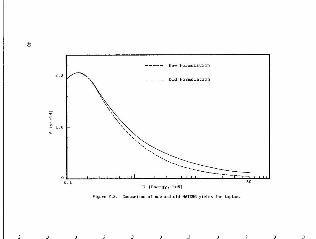
Comparison of new and old MATCHG yields for kapton ••••• • • • • • • • • •
Comparison of new and old MATCHG yields for aluminum .••••••••
Three nested octagons • • •
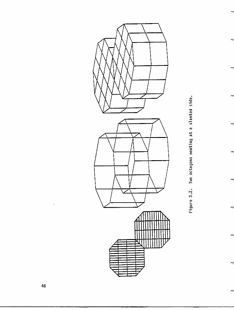
Two octagons meeting at a slanted side
Geometry for electron gun aimed at a sphere •• . . . • . • . . • . . • •
Geometrical quantities used to calculate current density ••••.••••••
Potential contours - cylindrical tank of radius 10 grid units about Z-axis ••
Potential contours - cylindrical tank of radius 10 grid units about Z-axis •.
~
27
30
30
40
41
45
46
52
55
67
68
The projection of an incident vector r upon the surface normal, in the "fan-like" coordinated system •• . • • • • • • • • •. 71
Anisotropic flux distribution with R = -0.35 .•••••...••••
Anisotropic flux distribution with R = -0.10 • • • • • • • •• • •••
Isotropic flux distribution •.
Anisotropic flux distribution with R = 0.10 ••••••••••
Anisotropic flux distribution with R = 0.50 . . . . . . . . . .
tv
78
79
80
81
82
-
Figure No.
3.13
5.1
LIST OF FIGURES (Concluded)
File examples for DETECT and ANISOTROPIC fluxes ••••••••• • 85
Block di agram of MATCHG • • • • • • • • • • 105
v
Table No.
2.1
2.2
2.3
2.4
2.5
2.6
3.1
3.2
4.1
4.2
5.1
5.2
5.3
5.4
5.5
LIST OF TABLES
Page
New, Revised, and Obsolete Option Words 18
Four Parameter Stopping Power Fits 34
Three Parameter Stopping Power Fits • . 34
Comparison of Three and Four Parameter Fits With ATAR • • • • • • • • • • • • 35
Comparison of Old and New Version Yields • 38
Secondary Yield for 1 keV Ions on Mo 43
Syntax ••• • • • •
Example of a DIRECT Data File.
NASCAP-Pseudo Graphics Subroutines
IGS and DISSPLA Routines Called by NASCAP
84
93
95
and PLOTREAD • • • • • •• 98
MATCHG COllll1ands
Command Formats
Initial Default Values
User/Code Interfacing Routines
Material Properties .
vi
101
102
104
106
116

SUMMARY
NASCAP is a computer code that comprehensively analyzes problems of spacecraft charging. Using a fully three-dimensional approach, it can accurately predict spacecraft potentials under a variety of conditions. Under Contract No. NAS3-22536 several revisions and a few extensions were implemented with a view toward making NASCAP more powerful and easier to use. Among the extensions are a multiple electron/ion gun test tank capability, and the ability to model anisotropic and time-dependent space environments. These extensions and revisions are documented in this volume.
Also documented here are a greatly extended MATCHG program and the preliminary version of NASCAP/LEO. The interactive MATCHG code has been developed into an extremely powerful tool for the study of material-environment interactions. NASCAP/LEO, a three-dimensional code to study current collection under conditions of high voltages and short Debye lengths, has been distributed for preliminary testing.
There are two companion volumes to this report. Volume II, NASA CR-167856, contains chapters entitled "Validation of the NASCAP Model Using Satellite Data", "NASCAP Applications Guide", "Differential Charging of High-Voltage Spacecraft: The Equilibrium Potential of Insulted Surfaces", and "Large Space Structure Modeling". Volume III, NASA CR-167857, documents a computer code for the modeling of plasmas external to ion thrusters.
1

.....
2
.--,.
1. INTRODUCTION
This is the final report on the NASCAP code development tasks (Tasks 1 and 2) of Contract No. HAS3-22536, "Additional Extensions to the tlASCAP Computer Code". The \'lOrk \,/as performed by Systems, Sci ence and Software beb/een 29 September 1980 and 30 September 1981.
This report includes information from monthly reports published throughout the contract period, as well as some new items. There are blo other volumes of the final report. Volume II, "Ion Thruster Code Manual", documents the preliminary version of a two-dimensional (R-Z) model for calculating plasma densities, current densities, potentials, and temperatures in the plasmas external to an ion thruster (Task 7). Volume III, "Validation of the ~JASCAP SCATHA r10del", describes research directly related to the SCATHA spacecraft (Task 3).
NASCAP/GEO (NASA fharging ~nalyzer frogram/geosynchronous Iarth .Q.rbit, henceforth referred to as tJASCAP) is a pm/erful computer program for studying spacecraft charging. It is intended as a tool for spacecraft designers to help them avoid the problems of electrical charging in space, and for scientific experimenters to aid in the design and interpretation of flight experiments. As there is now a group of researchers using NASCAP on a day-to-day basis, the emphasis of this year's work was on consolidation and validation rather than on extension.
The work directly related to the NASCAP/GEO co~e has ~een divided somewhat arbitrarily into revisions (described in Chapter 2) and extensions (described in Chapter 3). The revisions (Chapter 2) are those changes intended to promote ease of installation, use, and interpretation. The largest task in this category \las conversion from FORTRAN V to ASCII FORTRAN. Other revisions included production of a NASCAP Pocket Guide, revision of the RDOPT input, sUbstantial review and revision of the code output, and a review of NASCAP's treatment of
3
secondary electron production. Extensions to NASCAP (Chapter 3) include revision of the treatment of right triangles in OBJDEF to allow definition of previously illegal objects; replacement of the previous, unsatisfactory, discharge simulation; incorporation of a fast-running mUltigun test tank environment; and extension of the space environment to allow anisotropic and time-dependent f1uxes.
Chapters 4, 5 and 6 deal with codes auxiliary to NASCAP. NASCAP*PLOTREAD (Chapter 4) is a graphics interface routine which has enhanced the transferability of NASCAP to other installations. NASCAP*~~TCHG (Chapter 5) has been enhanced to make it a very powerful, fast-running, interactive tool for the study of material-environment interactions. NASCAP*TER~lTALK (Chapter 6) has been extended to give flux breakdown printouts.
Chapter 7 describes the NASCAP/LEO (NASCAP/!:.o\'1 Iarth Qrbit) code. A preliminary version of this code has been installed at NASA/LeRC.
The appendices include a list of IlASCAP-related reports and publications, as well as several publications written under this contract.
4
2. NASCAP/GEO REVISIONS
2.1 CONVERSION TO ASCII FORTRAN
The first major undertaking of this year's contract was conversion of the NASCAP code from UNIVAC FORTRAN V to ASCII FORTRAN. Among the reasons for this conversion were:
1. Demands by NASA/LeRC systems personnel. 2. Impending unavailability of a FORTRAN V plot library at
S-Cubed. 3. Hopes for shortened execution time and improved diagnostics. 4. Closer approach to IBM compatibility.
It was elected to eschew the new, allegedly advantageous, features of ASCII FORTRAN (e.g., character variables, if-then-else logic, offset array subscripts) as these are imperfectly implemented and not CDC compatible. Rather, the needed changes were, as much as possible, made line by line. Nonetheless, the discovery of residual conversion errors continued for several months after the ASCII version was declared the official version of NASCAP. This shows that the compiler dependence of coding can often be rather subtle.
The FORTRAN V-ASCII FORTRAN difference affecting by far the greatest number of lines of code is the representation of literals. FORTRAN V represents literals in words of six FIELDATA characters, while ASCII FORTRAN uses words of four nine-bit ASCII characters. We elected to make NASCAP literals four-character significant. A few exceptions (TANKCUR, TANKTRAJ, PATCHW, PATCHR) were made eight-character significant.
We were then left with a language quirk to deal with. While the statement
A = IBI
is legal, the statement IF (A.EQ.IB I ) •
5
,
is arbitrarily declared illegal in ASCII FORTRAN. The initial idea to circumvent this was to use
IF (XOR(A,'B').EQ.O) • The problem which quickly arose was that A might inadvertently contain lower case letters. Therefore a new subroutine, XORR, was written which converted both arguments to upper case before comparing. The code conversion was accomplished using XORR for literal compares. However, this syntax proved rather awkward. Accordingly, logical function routines EQUAL and NOTEQL were written, and all new coding uses those routines (which call XORR) for literal compares.
The different representation of literals also affected FORMAT statements and array lengths. Numerous AS's had to be changed to A4 1 s, and arrays had to be lengthened to accommodate fewer letters per word. (The latter constituted a large portion of the residual conversion problems.) Many FORMAT statements were also affected by different printing of numbers under lEI conversion.
A few assembly language subroutines (S3MCOR, TIMLFT, FASTIO) were originally written with the FORTRAN V protocol. These routines were left unchanged, necessitating the use of EXTERNAL* entrypoint statements in the calling routines.
NASCAP's dynamic storage allocation (S3MCOR) was found to conflict with ASCII FORTRAN's dynamic allocation of I/O buffers. This necessitated writing an assembler routine F2FCA to provide buffers in the main segment. Since the resulting buffer space was limited, care had to be taken to avoid gratuitously opening files, and to close files after use. In a related matter, the FORTRAN V NTABZ was replaced with an equivalent ASCII FORTRAN F2FRT.
The segmentation structure carried over surprisingly intact. One necessary change was that the ASCII FORTRAN diagnostic routings (FTNPMD) were too large to remain in the main segment. They were put, along with RETRNO, in a higher segment.
S

As part of the conversion, a neutral graphics concept was introduced into NASCAP. NASCAP nO\'I writes a sequence of dummy graphics calls on file 2. A postprocessor (NASCAP*PLOTREAD.) reads these dummy calls and interfaces to the user's graphics library. This feature is discussed in more detail later in this report. Another added feature was automatic assignment of scratch files.
The ASCII FORTRAN version of NASCAP was compiled and tested at S-Cubed using level 9Rl of ASCII FORTRAN. All routines were compiled with the options FZE. In one instance the compiler generated bad code. The problem was corrected by rewriting the line. The code was installed at NASA/LeRC under level 7Rl. It was found that:
1. Many routines required minor syntactical changes. 2. Some routines caused the compiler to guard mode if the
Z-option was used. 3. Some routines caused the compiler to loop if the Z-option
was not used. 4. A successful collection (@MAP) required that the bulk of
routines be compiled with the Z option and without the F option.
5. The ERR= branch on I/O and DECODE statements was highly unreliable.
6. Several routines generated incorrect code when compiled with the Z option. The conditions were corrected by substituting the V option.
As a result, there is no uniform set of compilation options under level 7Rl. We conclude that level 7Rl of ASCII FORTRAN is totally unsati sfactory.
7

2.2 NASCAP POCKET GUIDE
Early in the contract period we issued a NASCAP Pocket Guide to serve as a convenient memory aid to NASCAP options and syntaxes. The Guide has proved extremely worthwhile. Here we reprint the Guide, together with some errata and updates. Card-stock copies of the Guide are available on request from Systems, Science and Software.
2.2.1 NASCAP Pocket Guide
NASCAP
POCKET GUIDE NOVEM SER 1, 1980
This document IS a qUick reference gUide for the experienced user of NASCAP-the NASA Charging Analyzer Program It contains common NASCAP syntax and examples
There are also several interactive computer programs for easy pre· and post·processlng of NASCAP information For descriptIOns of these and further NASCAP documentation, see NASA publications CR·159417 (NASCAP Users Manual) and CR·159595 (Final Report 1979)
8
.......

USER OPTIONS-FILE 26 Supplied In file 26-0PT file In this section. "'" Indicates Integers "< >" indicates optional Input Eilloses" "
Indicate continue on same line The most Important options are RESTART. DELTA. LONGTIMESTEP. NCYC. and MESH Options are set sequentially as read They are remembered throughout the steps of a NASCAP execution. and may be changed by RODPT calls at any time
SYNTAX MEANING DEFAULT EXAMPLE 3D·VIEW x y z new SATPlT view 3 default ViewS 3D·VIEW 4 2 49 8 3D VIEW NONE clear view table 3 default views 3D·VIEW NONE APRT gr,dsl!l number grids potential print 1 APRT2 BFIElD bx by bz constant mag field-Webers/m' 0,0,0 BFIElD aIlE 5 1 E·5 BIAS condl!l volts conductor bias relative to no bias BIAS 2 ·500
conductor 1 CIJ condalJl condb' farads mutual conductor capacitance stray capacitance only CIJ341E4 COMMENT <anything> comment-no effect none COMMENT SEPT 25 CHANGES CONTOURS NONE clear contour table no contours CONTOURS NONE CONTOURS STANDARD 3 center cuts no contours CONTOURS STANDARD
CONTOURS G) cutl!l additional contour cut no contours CONTOURS Y·l GRIDS 3 MOD 4
<GRIDS ngl!l MOD mod'>
CONTOURS G) cutl!l OFF clear specific cut no contours CONTOURS X a OFF
CONVEX convex oblect self shadowing only HIDCEl must be called for CONVEX nonzero sun IntenSity
CONVERGENCE PLOTS ON potential solver printer plots on CONVERGENCE PLOTS ON CONVERGENCE PLOTS OFF CONVERGENCE PLOTS OFF
DEADLINE hhmmss' finish before lime of day none DEADLINE 234500 DEBYE activates Debye screening no screening DEBYE DELFAC factor tlmestep = tlmestep • factor 1 DELFAC 1 5 DELTA tlmestep Inilial tlmestep (seconds) DELTA 01 DIPOLE MOMENT px py pz magnetic dipole moment (A - M') none DIPOLE MOMENT 1 E·2, 1 E 2, a AT
AT x y z and locallon 0,0 5 DISCHARGE relax perform discharge analysIs no discharge analysIs DISCHARGE 5
EFFCON ON eff~ctlve surface conductIVIty off EFFCON ON EFFCON OFF EFFCON OFF
EMITIER u",,1JI acllvate parllcle emitter NOEMIT EMITTER 23 END end of Input file none END FIXP condlJl volts fiX conductor pot entiat conductor floats FIXP 2 ·3000 FLOAT remove all prevIous FIXP and BIAS prevIous status FLOAT FLOAT cond' float preVIOUSly fixed or prevIous status FLOAT 3
biased conductor
IOUTER (~) a-grounded outer boundary 2 I e IIr potenllals IOUTER 2 2-monopole outer boundary
9

SYNTAX MEANING DEFAULT EXAMPLE LONGTIMESTEP <dvllm> ImpliCit charging NOLONG LONGTIMESTEP 2000
<voltage limit per limestep>
MATVIEW ± G) cuta, cutbl additional matenal plot 6 default plots MATVIEW -Z -5 +5
MATVIEW NONE clears MATVIEW table 6 default plots MATVIEW NONE NCVC steps' number limesteps to run 1 NCYC 5 NG gnds' number computational gnds 2 NG 3 NOEMIT turn off previously defined emiller prevIous status NOEMIT NOLONG see LONGTIMESTEP expliCit charging NOLONG NOPRINT modulename see PRINT no extra printout NOPRINT POTENT NOSCALE see SCALE SCALE NOSCALE NOSHEATH see SHEATH no sheath plot NOSHEATH NOTIME see TIMER no limer NOTIME NZ zdlvl z grid size 33 NZ29 ') OFFSET xii y, zl moves coordinate ongln center of mesh (9 9 17) OFFSET 0 0 0 POTCON decades convergence of potential solver 8-CAPACI, 4-TRILIN POTCON 3 PRINT modulename diagnostic prints, modulename NOPRINT PRINT POTENT
IS LlMCEL POTENT HIDCEL or OBJDEF
REPEAT times' plot repetition factor (IGS only) 1 REPEAT 3 RESTART next tlmestep-old problem new problem RESTART SCALE potential solver scales potential SCALE SCALE ,....
and boundary conditions
SECONDARV <EMISSION> ANGLE secondary formulation ANGLE SECONDARY ANGLE SECONDARY <EMISSION> NORMAL secondary formulation ANGLE SECONDARY EMISSION NORMAL SHEATH plot space charge denSity NOSHEATH SHEATH SUNDIR x y z sun direction vector I, I, 1 SUNOIR I, D, 25 SUNINT Intens sun Intensity 0 SUNINT08 SURFACE CORNER xl y, Z' surface cell of Interest none SURFACE CORNER 3, 3, 2 -1,0,0
<norxl noryl norzl> SURFACE CELL cellI surface cell of Interest cell f1 SURFACE CELL 541
TANKCUR OFF tank current contour plots off TANKCUROFF TANKCUR ON TANKCURON
TANKTRAJ OFF tank particle traJectory plots off TANKTRAJ OFF TANKTRAJ ON TANKTRAJ ON
TIMER execution time each module NOTIME TIMER ....., XMESH Unit phYSical grid spacing (meters) 01 XMESH 03 ZTRUNCATE zlo' zhll truncation of outer grid full gnd, -16 to + 16 ZTRUNCATE -12 +12
......
10

NASCAP COMMANDS
IF NO UNIT PREREQUISITE MNEMONIC COMMAND WORD SPECIFIED ADDITIONAL INPUT COMMAND Aead Options ADOPT <unit> Umt 26 assumed Option keywords None Object Defimlton OBJDEF <uOll> Unit 20 assumed Object descnplton ADOPT Satellite Plot SATPLT None OBJDEF Capacitance CAPACI None OBJDEF Tnlanear Charge TAIUN <unat> Umt 22 assumed Flux definatlon CAPACI (HIDCEL) Hidden Cells HIDCEL None OBJDEF Aotate with Time AOTATE <unat> Use 1 APM about Z aXIs (2 cards) radians/sec, TAIUN
IOlltal sun vector Spin Average SPIN <unat> Eight views about Z aXIs (1 card) 'views, OBJDEF
spin aXIs vector Detector Enable DETECT <unit> Unit 5 (runstream) Detector keywords TRtUN
assumed (see Manuat) New Malenal Parameters NEWMAT <umt> Error (4 cards) matenal OBJDEF
parameters End Aun END None ADOPT
11
\
12
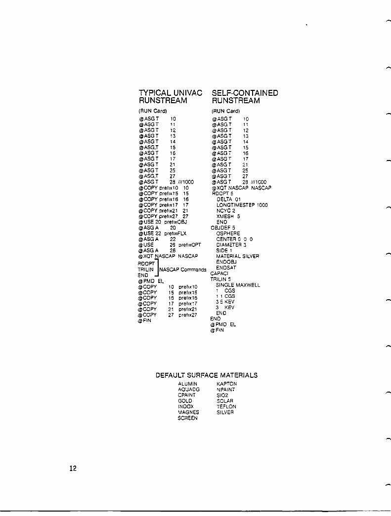
TYPICAL UNIVAC SELF·CONTAINED RUNSTREAM RUNSTREAM (RUN Card) (RUN Card)
@ASGT 10 @ASGT 10 @ASGT 11 @ASGT 11 @ASGT 12 @ASGT 12 @ASGT 13 @ASGT 13 @ASGT 14 @ASGT 14 @ASG,T 15 @ASGT 15 @ASGT 16 @ASGT 16 @ASGT 17 @ASGT 17 @ASGT 21 @ASGT 21 @ASGT 25 @ASGT 25 @ASG,T 27 @ASGT 27 @ASGT 28 1111000 @ASGT 28 1111000 @COPY prellx10 10 @XOT NASCAP NASCAP @COPY prellx15 15 RDOPT 5 @COPY prellx16 16 DELiA 01 @COPY preflx17 17 LONGTIMESTEP 1000 @COPY prellx21 21 NCYC 2 @COPY preflx27 27 XMESH 5 @USE 20 prellxOBJ END @ASGA 20 OBJDEF 5 @USE 22 preflxFLX OSPHERE @ASGA 22 CENTER 0 0 0 @USE 26 prellxOPT DIAMETER 3 @ASGA 26 SIDE 1 @XOT NASCAP NASCAP MATERIAL SILVER
RDOPT] ENDOBJ
TRILiN NASCAP Commands ENDSAT
END CAPACI
@PMD EL TRILiN 5
@COPY 10 prefix 10 SINGLE MAXWELL
@COPY 15 preflx15 1 CGS @COPY 16 preflx16 ' , CGS
@COPY 17 preflx17 35 KEV
@COPY 21 preflx21 3 KEV
@COPY 27 preflx27 END
@FIN END @PMD EL @FIN
DEFAULT SURFACE MATERIALS ALUMIN AOUADG CPAINT GOLD INDOX MAGNES SCREEN
KAPTON I\JPAINT SI02 SOLAR TEFLON SILVER
..-..

OBJECT DEFINITION-FILE 20 All Integer Input-except for "radius" and
. material name .. See NASCAP Users Manual for information on material parameters OBJECT DEFINITION OBJECT DEFINITION SYNTAX EXAMPLES RECTAN CORNER x y z DELTAS c.x c.y c.z (UP TO 6 SURFACE CARDS) ENDOBJ
WEDGE CORNER x y z FACE matenalname normal
(type 110) LENGTH c.x c.y c.z (UP TO 4 SURFACE CARDS) ENDOBJ
TETRAH CORNER x Y z FACE matenalname normal
(type 111) LENGTH c.x (UP TO 3 SURFACE CARDS) ENDOBJ
OCTAGON AXIS x Y z x v' z' WIDTH W SIDE s IUP TO 3 SPECiAL SURFACE
CARDS + or C)
ENDOBJ , BOOM AXIS x y Z x v z' RADIUS radiUS (floating pOint) SURFACE matenalname ENDOBJ
OSPHERE CENTER x y z DIAMETER d SIDE S MATERIAL matenalname ENDOBJ
RECTAN CORNER 3 -2 8 DELTAS 1 2 4 SURFACE +X ALUMINUM SURFACE - X ALUMINUM SURFACE + Y ALUMINUM SURFACE - Y ALUMINUM SURFACE + Z ALUMINUM SURFACE - Z ALUMINUM ENDOBJ
WEDGE CORNER -3 2 1 FACE SI02 - 1 - 1 0 LENGTH 1 1 3 SURFACE + X SI02 SURFACE + Y SI02 SURFACE + Z GOLD SURFACE - Z SI02 ENDOBJ
TETRAH CORNER -3 -2 8 FACE KAPTON 1 1 - 1 LENGTH 2 SURFACE - X TEFLON SURFACE - Y KAPTON SURFACE - Z TEFLON ENDOBJ
OCTAGON AXIS 3 2 - 6 3 2 - 9 WIDTH 3 SIDE 1 SURFACE + SILVER SURFACE - SILVER SURFACE C MAGNES ENDOBJ
BOOM AXIS 0 6 0 0 12 0 RADIUS 25 SURFACE ALUMINUM ENDOBJ
QSPHERE CENTER 0 0 0 DIAMETER 4 SIDE 2 MATERIAL NPAINT ENDOBJ
OBJECT DEFINITION OBJECT DEFINITION SYNTAX EXAMPLES FILlll CORNERLINE x y Z x y' z' FACE matenalname normal
(type 111) ENDOBJ
PLATE CORNER x y z DELTAS c.x c.y c.z
TOP :: (~) matenalname
BOTTOM:: G) matenalname ENDOBJ
PATCHR CORNER x y z DELTAS c.x c.y c.z (Up TO 6 SURFACE CARDS) ENDOBJ
PATCHW CORNER x y z FACE matenalname normal
(type 110) LENGTH c.x c.y c.z (UP TO 4 SURFACE CARDS) ENDOBJ
FILlll CORNER 3 2 6 - 5 4 6 FACE SOLAR - I - 1 - 1 ENDOBJ
PLATE CORNER -1 - 1 - 10 DELTAS 2 2 0 TOP + Z CPAINT BOTTOM - Z CPAINT ENDOBJ
PATCHR CORNER 3 -2 8 DELTAS 1 0 1 SURFACE - Y SCREEN ENDOBJ
PATCHW CORNER -3 2 7 FACE AQUADG - 1 LENGTH 1 1 1 ENDOBJ
-1 0
NOTES normal IS three values each either + t 0 or - 1
SURFACE CARD has the fOllOWing format
SURFACE :: G) matenalname
SPECIAL SURFACE CARD IS
SURFACE (e) matenalname
OTHER OBJECT DEFINITION COMMANDS EN DSAT COMMENT OFFSET I J k CONDUCTOR n
DELETE I J k unrecognized word
Must be last card In file No effect Moves coordinate ongln Sets number of underlYing conductors (Is... n ~7) Deletes surfaces leaVing empty cell Assumed to be name of new surface matenal Next card scanned for parameters
13

14
FLUX DEFINITION-FILE 22 SINGLE MAXWELLIAN SYNTAX
MAXWELL eldens densltyunlts prdens denSllyunlls eltemp tempunllS pnemp tempunlts END
DOUBLE MAXWELL SYNTAX DOUBLE MAXWELL ELECTRONS eldens eenSltyUnlls ellemp tempunlts ELECTRONS eldens denSllyunllS eltemp tempunlts PROTONS preens densllyunlts prtemo tempunlts PROTONS prdens denSltyunllS prtemp tempunlts END
SINGLE MAXWELLIAN EXAMPLE MAXWELL 1 CGS 1 E6 MKS 3000 EV 35 KEV END
DOUBLE MAXWELLIAN EXAMPLE DOUBLE MAXWELL ELECTRONS 03E6 MKS 10 KEV ELECTRONS 0 7 eGS 500 EV PROTONS 0 3 CGS 1 E6 KELVIN PROTONS 07E.6 MKS 1 E·15 JOULES
The denSltyunlts are MKS or eGS and tempunlts are JOULES EV KEV ERGS or KELVIN For test tank flux see Users Manual
DEFAULT FILE NUMBERS-FILE NAMES-FILE USAGE
USER INPUT FILES 26 prefix OPT user options 20 prefix OBJ object definition 22 prefix FLX flux definition
RESTART FILES 10 IP potential 15 IROUS charge 16 IPQCND TERMTALK Information 17 ILTBL element table 21 ICNOW various-used everywhere 27 IAREA booms
SCRATCH FILES 11 IAUN conjugate gradIent 12 IR conjugate gradIent 13 IU conjugate gradient 14 ISPARE conjugate gradient 25 IDIV conjugate gradIent 28 IPART plots
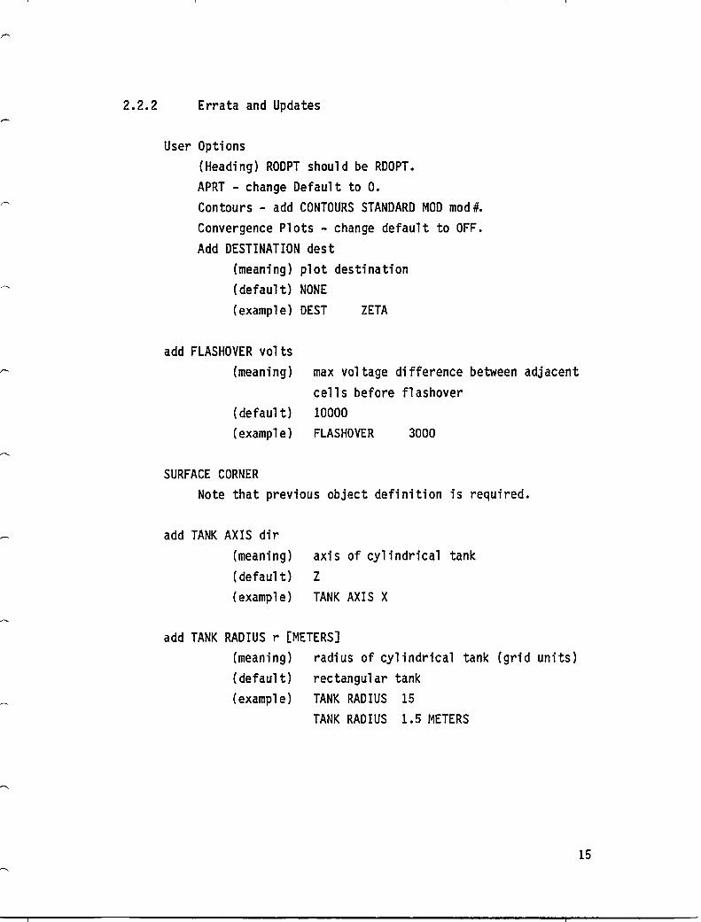
2.2.2 Errata and Updates
User Options (Heading) RODPT should be RDOPT. APRT - change Default to o. Contours - add CONTOURS STANDARD MOD modi. Convergence Plots - change default to OFF. Add DESTINATION dest
(meaning) plot destination (default) NONE (example) DEST ZETA
add FLASHOVER volts (meaning) max voltage difference between adjacent
cells before flashover (default) 10000 (example) FLASHOVER 3000
SURFACE CORNER Note that previous object definition is required.
add TANK AXIS dir (meaning) (default) (example)
axis of cylindrical tank Z
TANK AXIS X
add TANK RADIUS r [METERS] (meaning) (defaul t) (example)
radius of cylindrical tank (grid units) rectangular tank TANK RADIUS 15 TANK RADIUS 1.5 METERS
15
16
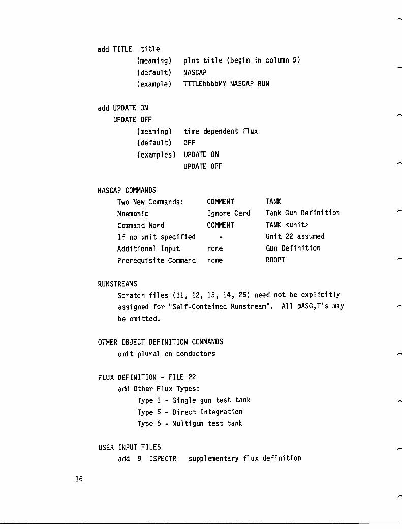
add TITLE ti tl e (meaning) (defaul t) (example)
plot title (begin in column 9) NASCAP TITLEbbbbMY NASCAP RUN
add UPDATE ON UPDATE OFF
(meaning) (defaul t)
time dependent flux OFF
(examples) UPDATE ON UPDATE OFF
NASCAP COMMANDS Two New Commands: COMMENT Mnemonic Ignore Card Comnand Word COMMENT If no unit specified Additional Input none Prerequisite Command none
RUNSTREAMS
TANK Tank Gun Definition TANK <unit> Unit 22 assumed Gun Defi niti on RDOPT
Scratch files (11, 12, 13, 14, 25) need not be explicitly assigned for "Self-Contained Runstream". All @ASG,T's may be omitted.
OTHER OBJECT DEFINITION COMMANDS omit plural on conductors
FLUX DEFINITION - FILE 22 add Other Flux Types:
Type 1 - Single gun test tank Type 5 - Direct Integration Type 6 - Multigun test tank
USER INPUT FILES add 9 ISPECTR supplementary flux definition
......
2.3 OPTION REVISIONS
During this contract year the NASCAP options were revised with a view toward making them easier to use and to have more reasonable defaults. In many cases new syntaxes were added to perform in a superior fashion the functions of existing options, while retaining the older syntaxes for downward compatibility. In two cases (APRT and ICNVP) defaults were changed to eliminate non-useful printing. Also, new options were added to implement the NASCAP extensions developed under this contract. A list of new, revised, and obsolete option words is provided in Table 2.1.
2.3.1 Justifications for New Options
The new options break down into four categories: coordinate system, name changes, structural changes, and extensions.
COORDINATE SYSTEM - The original NASCAP coordinate system numbered each grid 1 to 17 in the X and Y directions, and 1 to 33 in the Z direction. The newer, more intuitive system puts the origin at grid center, so Z coordinates go from -16 to +16. These two incompatible systems coexist in NASCAP and confuse everybody. Some user options (e.g., SURFACE AT) required the user to use the 1-33 system. The new commands (e.g., SURFACE CORNER) allow a choice of coordinate systems, through the use of an OFFSET command.
NAMES - Some option names (e.g., ITCUR) gave the user only a foggy notion of what they were for. The new option names (e.g., TANKCUR) are more informative.
STRUCTURE - The plotting options NCON, NDIR, and NDIV were unnecessarily complicated and restrictive. The new options (CONTOURS, 3D-VIEW, and MATVIEW) give more control over plots and are easier to use.
17

TABLE 2.1. NEW, REVISED, AND OBSOLETE OPTION WORDS
NEW FLUX SPECIFICATIONS
MAXWELLIAN DOUBLE MAXWELLIAN TYPE 5 (Direct Integration) TYPE 6 (Multigun Test Tank)
NEW OPTION KEYWORDS
1. Coordinate Systems DIPOLE MOMENT OFFSET SURFACE CORNER ZTRUNCATE
2. Mnemonic Names CONVERGENCE PLOTS TANKCUR TANKTRAJ
3. Structural Simplification CONTOURS MATVIEW 3D-VIEW
4. Extensions
18
DES TI NA TI ON FLASHOVER TANK AXIS TANK RADIUS TITLE UPDATE
EXCLUDED OPTION KEYWORDS
1.
2.
3.
Superseded Keywords NGPLOT --> CONTOURS ICON --> CONTOURS ICNVP --> CONVERGENCE PLOTS ITPART --> TANKTRAJ rTCUR --> TANK CUR IROUSP --> SHEATH MAXITR --> POTCON NCON --> CONTOURS NDIR --> 3D-VIEW NDIV --> MATVIEW SURFACE AT --> SURFACE CORNER TANKSIZE --> ZTRUNCATE NGPRT --> APRT DIPOLE --> DIPOLE MOMENT
Rarel y Used MCYC DSCALE SHEATH SELF CONSISTENT PROGID (CDC only) IP, IR, IDIV, IV, rSPARE, IROUS,
IOBJ, IOBPLT, ISAT, IPQCND, ILTBL, ICNOW, IKEYWD, IFLUX, IAREA, IPART (file numbers)
Functionally Obsolete NX NY ICREST IPREST

EXTENSIONS - New options associated with the discharge revision, environment extensions, and plotting revisions.
2.3.1.1 Flux Definition. In addition to the new user options, two flux type specifications have been added. 1 MAXWELLIAN 1 and 'DOUBLE MAXWELLIAN 1 will perform the same function as 'TYPE 21 and 'TYPE 41
,
respectively.
Test tank (Type 1) and particle pushing (Type 3) flux types were not included on the Pocket Guide for reasons of space. Direct integration (Type 5), mUltigun test tank (Type 6) postdated the Pocket Guide.
2.3.1.2 Options Not Documented. Several options from the NASCAP User's Manual were not included in the Pocket Guide. These option keywords were left out for anyone of these reasons:
1. Superseded by another (e.g., MAXITR replaced by POTCON). 2. Rarely or never used (e.g., file number keywords). 3. Reference obsolete functions (e.g., ICREST).
2.3.2 Description of New Options
CONTOURS NONE CONTOURS STANDARD <MOD modi>
CONTOURS (ZXy ) cut# <GRIDS ng# MOD modi>
CONTOURS (zXy) cut# OFF
Determines contours to be plotted after each potential cycle. Replaces NCON, ICON, NGPLOT and the additional cards following NCON.
Allows complete user control over potential contour plots.
19
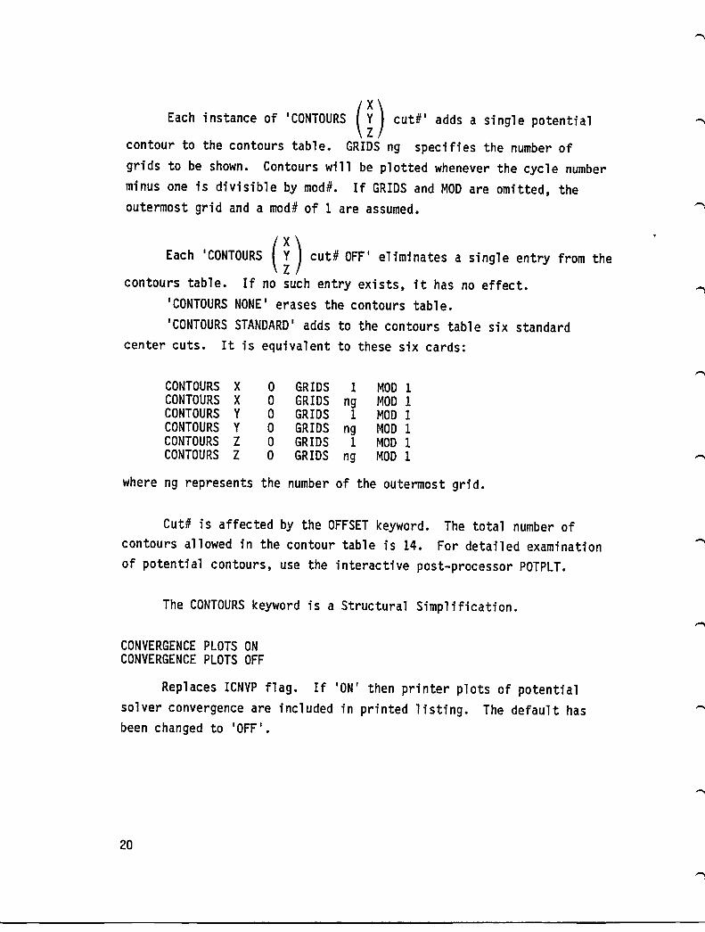
Each instance of 'CONTOURS (~) cud' adds a single potential
contour to the contours table. GRIDS ng specifies the number of grids to be shown. Contours will be plotted whenever the cycle number minus one is divisible by modi. If GRIDS and MOD are omitted, the outermost grid and a modi of 1 are assumed.
Each 'CONTOURS (~) cud OfF' eliminates a single entry from the
contours table. If no such entry exists, it has no effect. 'CONTOURS NONE' erases the contours table. 'CONTOURS STANDARD' adds to the contours table six standard
center cuts. It is equivalent to these six cards:
CONTOURS X 0 GRIDS 1 MOD 1 CONTOURS X 0 GRIDS ng MOD 1 CONTOURS Y 0 GRIDS 1 MOD 1 CONTOURS Y 0 GRIDS ng MOD 1 CONTOURS Z 0 GRIDS 1 MOD 1 CONTOURS Z 0 GRIDS ng MOD 1
where ng represents the number of the outermost grid.
Cut# is affected by the OFFSET keyword. The total number of contours allowed in the contour table is 14. For detailed examination of potential contours, use the interactive post-processor POTPLT.
The CONTOURS keyword is a Structural Simplification.
CONVERGENCE PLOTS ON CONVERGENCE PLOTS OFF
Replaces ICNVP flag. If 'ON' then printer plots of potential solver convergence are included in printed listing. The default has been changed to 'OFF'.
20
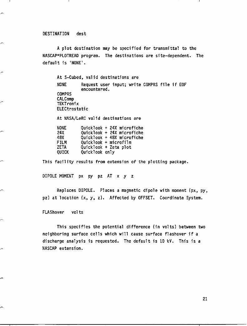
DESTINATION dest
A plot destination may be specified for transmittal to the NASCAP*PLOTREAD program. The destinations are site-dependent. The default is 'NONE'.
At S-Cubed, valid destinations are NONE Request user input; write COMPRS file if EOF
encountered. COMPRS CALComp TEKTronix ELECtrostatic
At NASA/LeRC valid destinations are
NONE Quicklook + 24X microfiche 24X Quicklook + 24X microfiche 48X Quicklook + 48X microfiche FILM Quicklook + microfilm ZETA Quicklook + Zeta plot QUICK Quicklook only
This facility results from extension of the plotting package.
DIPOLE MOMENT px py pz AT x Y z
Replaces DIPOLE. Places a magnetic dipole with moment (px, py, pz) at location (x, y, z). Affected by OFFSET. Coordinate System.
FLAShover volts
This specifies the potential difference (in volts) between two neighboring surface cells which will cause surface flashover if a discharge analysis is requested. The default is 10 kV. This is a NASCAP extension.
21

MATVIEW !. ( ~) cutaH cutb#
MATVIEW NONE
Determines material plot views. Replaces NDIV and 1 to 6 cards following NDIV with 1 to 11 entries each.
When SATPLT is called, material plots are automatically generated. If the MATVIEW keyword has not been used, six default views will be generated.
Each material plot shows all the surface one would see looking from the specified direction. Cuta# and cutb# give limits, outside of which all surfaces are made invisible. This is handy for examining concave objects.
'MATVIEW NONE' clears the material views table, eliminating the default views and any other previously defined views.
'MATVIEW !. ( ~) cutaH cutbH' adds one view to the material
views table, up to a maximum of five per direction, or 30 total. Cuta # and cutb # are affected by the OFFSET keyword.
Assuming that OFFSET has not been used, the following set of keywords is equivalent to not using MATVIEW at all:
MATVIEW NONE MATVIEW +X -8 8 MATVIEW -x -8 8 MATVIEW +Y -8 8 MATVIEW -Y -8 8 MATVIEW +Z -16 16 MATVIEW -Z -16 16
The MATVIEW keyword is a Structural Simplification.
22

OFFSET x# y# z#
New keyword option. Allows user to place coordinate origin for RDOPT options. Works just like OFFSET command in Object Definition file. OFFSET during OBJDEF has no effect on OFFSET during RDOPT. New origin location is specified in "absolute" (1-33) coordinates. For example, specifying 10FFSET 0 0 01 sets up the old NASCAP (1-17, 1-17, 1-33) coordinate system. Default offset is at mesh center, i.e., 10FFSET 9 9 171 for the usual mesh. OFFSET should be placed first, or near the front of the OPT file, before other options affected by it. Coordinate System.
SURFACE CORNER x# y# z# <norx# nory# norz#>
Replaces SURFACE AT. Specifies surface cell for extra charging printout. x, y, and z are the coordinates of the lower left corner of the volume element out of which the surface points. Optionally, a surface normal can be specified, to distinguish between cells on the same element. (For geometrically complex objects, use TERMTALK to find the cell number and use 'SURFACE CELL cell#I.) The coordinate system is as specified by OFFSET, with default the "centered" (-16 to +16) system. This is the only difference between SURFACE AT and SURFACE CORNER. SURFACE AT uses the 1 to 33 coordinate system exclusively. (Note: Either keyword can only be used if OBJDEF has already been called; e.g., in a RESTART run.) Coordinate System.
TANK AXIS (~)
The axis for a cylindrical tank may be specified. The default is Z. This option results from a NASCAP extension.
23

TANK CUR ON TANK CUR OFF
Replaces ITCUR flag. If 'ON' then test tank current contour plots are output on graphics device. Mnemonic Aid.
TANK RADIUS x <METERS>
The radius of a cylindrical tank may be specified in grid units or meters. The default is a rectangular tank. This option also guarantees a grounded outer boundary. This is a NASCAP extension.
TANKTRAJ ON TANKTRAJ OFF
Replaces ITPART flag. If 'ON' then test tank particle trajectory plots are output on graphics device. Mnemonic Aid.
TITLE title
A title to appear on the first plot frame (along with the date and time) may be specified beginning in column 9 of the input line. The title may have up to 56 characters. The default title is 'NASCAP'. This option results from extension of the plotting package.
UPDATE
The update feature allows the description of the plasma spectrum used by the code to be changed automatically to the most recent one available, drawn from a list of spectra and their associated time periods. For example, given a list of double Maxwellian spectra associated with successive 209 periods, as the accumulated timesteps exceed multiples of 205, the active plasma spectrum is updated to the most recent in the list. UPDATE is a NASCAP extension.
24
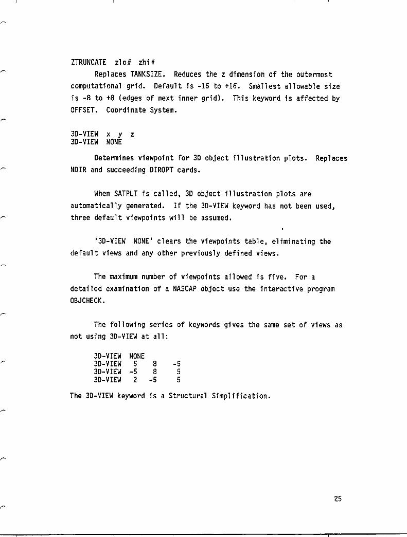
ZTRUNCATE zlo# zhi# Replaces TANKSIZE. Reduces the z dimension of the outermost
computational grid. Default is -16 to +16. Smallest allowable size is -8 to +8 (edges of next inner grid). This keyword is affected by OFFSET. Coordinate System.
3D-VIEW x y z 3D-VIEW NONE
Determines viewpoint for 3D object illustration plots. Replaces NDIR and succeeding DIROPT cards.
When SATPLT is called, 3D object illustration plots are automatically generated. If the 3D-VIEW keyword has not been used, three default viewpoints will be assumed.
'3D-VIEW NONE' clears the viewpoints table, eliminating the default views and any other previously defined views.
The maximum number of viewpoints allowed is five. For a detailed examination of a NASCAP object use the interactive program OBJCHECK.
The following series of keywords gives the same set of views as not using 3D-VIEW at all:
3D-VIEW 3D-VIEW 3D-VIEW 3D-VIEW
NONE 5 8
-5 8 2 -5
-5 5 5
The 3D-VIEW keyword is a Structural Simplification.
25

2.4 OUTPUT REVISIONS
NASCAP's printed output was reviewed and revised in order to reflect more clearly the input, the final result, and the physical processes leading thereto. In particular:
26
a. The option summary routine, SUMOPT, was rewritten to summarize options in a more clearly organized fashion and to be more indicative as to the option words available (Figure 2.1).
b. The format of the surface cell potential list was improved. Also, its initial values are printed for a RESTART run.
c. The output was clarified as to when a timestep begins and ends. Fluxes and currents were better defined as to initial or average values.
d. Units of current and charge were better defined. e. Initial values of low energy electron fluxes were printed
with limiting taken into account. f. Superfluous output in the LIMCEL section was made optional
or expunged. g. The defaults for convergence plot and grid potential array
printouts were changed to off.

HASA CHARGING A~ALYZER PROGRA" OPT ION SUMMARY
TITLE :HASCAP
GRID SIZE OPTIONS: HX NY 17 17
FULL OUTER GRID USED
HZ 13
NG 2
AOOITIOHAL OPTION WORDS: OFFSET, TANKSIZE, ZTRUNC
LOGICAL UNIT NUMBERS
INPUT FILES: IKEYwO Z6
ISAT 20
RESTART FllESI IP IROUS r 10 15
IFlUX 22
IPOCNO 16
ISPCTR 9
II. Tel ICNOW 17 21
UREA 27
SCRATCH FILESI lAUN JR 11 12 I~~V IU UPARE JOB.J IoePLT
1l 1'1 18 19
RUN MODE OPTIONS: ICREST IPREST NCYC MCYC o a 1 1
OELTA OtLFAC 1.00.000 1.00.000
OEADLIIIE : NONE AOOlfIONAL KEY.ORO : [RESTARTl
POTENTIAL SOLvtR OPTIONS: POTCON MAIITR 10uTER SCALt NOT SET 99 2 seal.
SCALING KEywORDS: SCALE, NOSCALt, OS=ALE AMBIENT SPACE CHARGE OPTION [KEYWORD DE8YE):NONE
CON~UCTOR FIXING AND BIASING:KEYWOAOS FIXP, BIAS, FLOAT
INTERCONDUCTOR CAPACITANCES: KEYWORD CI.J THE CODE UNIT OF CHAAGE IS 8.85_-013 CCULOMBS. THE COOL UNIT OF CAPACITANCE IS 8.aS-OIl FARADS. HO INTERCONOUCTOR CAPACITANCES SPEClFIED.
LONGTtMESTEP AND DISCHARGE OPTIONS ~~~~V1~~iT~~N~I!M~~JE~iE~O~~~~l!~E~~EP, OISCHARGE, FLASHOVER DISCHARGE AN'LYSIS OFF
ILLUMINATION SPECIFICATIONS: SUNINT: .000 SUNDIR: oS7n .S7H .577'1 SHADOWING FORMULATION (KEYWOAO:CONV(X]:SHAO
tNvIRONMENT TYPE ANO MESH SilE ITYPE: 2 UPOATE:OFF I"ESH: 1.00-001
SECONO'RT EMISSION FORMULATION :oANGl· EFFECTIvE PHOTOSHE'TH CONOUCTlvlTT (EFFCON] : OFF
OuTPUT OPTIONS I NGPRT (APRT] TIMER [NOTIMER]
o NO ICNVP [CONvERGENCE PLOTS): a
PRINT [NOPRINT]: POTENT LIHCEl OBJOEF NO NO SOHE
SUPFACE CELLS SPECIFIED FOR 1/0: I
HfDCEL NO
KETWOROS: CSUPFACE CELL], [SURFACt ATl, (SURFACE CORNtR]
PLOT OPTIONS: TlTLE=H.lSC.lP NGPLOT ICOH REPEAT ITPART ITCUR IROUSP
o a 1 a a 0 OES T : NONE NCON NDIR
(! l AOOITIONAL KEY.OROSI TANKCU~ r'NKTRA~ lD-YIEw ~ATYIEw CONTOUR
NO. OF AOOITIOHA~ CONTOUR PLOT CUTS: a NO. OF 3-0 PLOT vIEwS: 3
VECTORS FRO~ SATEL~ITE CENTER TOWARO vIEWER .RE
HO. or ~ATERIAL PlOT YIEws [NDIY] : 1 1
.SOOO -.sooo
.2000
1
.aooo .aooo -.5000
1
PARTICLE TRACKING OPTIONS: KEYWOROS, EHITTtR, NOEHITTER, SHEATH, SHEATH SELF-tONSISTENT
~O EHITTERS ~EouESTEO
HAGNETIC rIt~o OPTIONS: KEYwOqOS CSFIElO], COIPO~EJ CONSTAHT HAGHtTIC FIE~o:I .00 .00 NO MAGNETIC DIPOLES
.00
IPART 29
.5000
.SOOO
.SOOO
Figure 2.1. New format for NASCAP option summary, indicating default options.
27

2.5 SECONDARY ELECTRON REVIEW
2.5.1 A Reformulation of Secondary Electron Emission
NASCAP calculates the secondary electron emission yield, 0,
using the empirical formu1a:[1]
R
o = C f 1:X Ie-ax dx ( 2.1) o
where X is the depth of penetration of a primary electron beam into the material, and R is the "Range", or maximum penetration depth.
Equation (2.1) is based upon a simple physical mode1:[2] a. The number of secondary electrons produced by the primary
beam at a depth X is proportional to the energy loss of the beam or "stopping power" of the material, IdE/dxl.
b. The fraction of the secondaries that migrate to the surface and escape decreases exponentially with depth (f = eax ). Thus only those produced within a few multiples of the distance l/a (the depth of escape) from the surface contribute significantly to the observed yield.
The range increases with the initial energy, Eo' of the incident electrons in a way that approximates a simple "power 1aw .. :[3]
R = b En o
where 1.0 < n < 2.0.
28
(2.2)

Equation (2.2) implies a simple form for the stopping power S(E):
IdEI IdR I -1 E1-n
SeE) = Ox = ~ = rib (2.3)
Because the primary beam loses energy as it passes through the material, both E, and hence S(Eo'x), depend on the depth x. Integrating (2.3):
(2.4)
1 ( b ) l-l/n Sex) = rib r:-x (2.5)
The stopping power seE ,x) depends upon both the initial electron o energy Eo' via R, and the depth x. Figure 2.2a shows schematically SeE ,x) plotted against x for several values of E. Inspection of o 0 Figure 2.2 and Eq. (2.5) illustrates the following points:
1. S{Eo'X) increases with x, slowly at first, before reaching a singularity as x approaches R.
2. The initial value of S(Eo'x) decreases with increasing initial energy Eo'
Both of these observations are due to the decrease in electron-atom collision cross-section with increasing energy.
The yield is only sensitive to the details of the stopping-power depth-dependence for initial energies with ranges of the same order as the escape depth, R ~ l/a (i.e., about the maximum of the yield
29

30
s.. Ql :J 0
Co.
C' c ... c. c. 0 .. til
~ ~
til
EO 3
EO
Power Law E-Dependence
---- L~near~zed E-Dependence
4 J----!-4-----!------=----------------
Rl ~2 R3 R4
~----~~------~--------------------~--~A !-l/a --j "Depth of Escape"
Depth
Figure 2.2a. Energy deposition profiles of primary electrons for incident energies EO.
Inc~dent Energy EO
Figure 2.2b. Generalized yield curve.

curve). For lower energies, R « l/a, and essentially all of the primary energy is available for detectable secondary production, leading to a linear increase in yield with increasing Eo. At higher energies, where R » l/a, S(Eo'x) remains almost constant, at its initial value, over the depth of escape and so, along with S(Eo'x) the yield decreases as Eo increases.
NASCAP takes this into account and approximates the stopping power by a linear expansion in x, about x = O.
dE =(dR )-1 +(d2R) (dR )-3 x
dx dEo dE2" ~ o
(2.6)
NASCAP allows for a bi-exponential range law:
(2.7)
involving four parameters b1, b2, n1, n2• The parameters are fit to reproduce range data as accurately as possible. For materials where no suitable data is available, a mono-exponential form is generated using Feldman's empirical relationships,[3J connecting b and n to atomic data. The stopping power is then obtained indirectly via Eq. (2.6). Recently good theoretical estimates of the stopping power for a number of materials have become available[4J (see below). Comparison of these values with those implied by the range data showed significant discrepancies, particularly for those materials fit using Feldman's formula.[3J A better approach is to fit the four parameters in (2.7) directly to the stopping power data.
The method of fitting is described in Section 2.5.2.
31

Inspection of the tables of yields for the old and new input parameters shows that good agreement is found for most of the materials, particularly the metals. The major difference lies in the high energy "tail" of the kapton yield curve. The new version has a significantly damped high energy region compared with the old (e.g., the value at 50 keY is 3x higher for the old version). Damping also occurs for all but gold and teflon, by as much as 25 percent, in the high energy tail.
The effect of this will be to increase the charging rate of these materials (particularly kapton) for environments that sample these regions. Teflon is actually uniformly higher in the new version and so will charge at a slightly slower rate than before.
Experimental data[5] indicates that the original input parameters caused NASCAP to underestimate the rate of charging in some instances. These modified results may overcome this discrepancy.
The four parameters b1, b2, n1, n2, are fit to theoretical stopping power data rather than range data, providing a more direct contact between reliable information for IdE/dxl and the yield.
2.5.2 Fitting of Four Parameter Form to Stopping Power Data
The form:
is fit to the available data using the following algorithm:
32

1. E = 1.0 keY is taken as a fixed point and
2. Another fixed pOint is chosen - usually at or close to E • (If E ~ 1.0 keY another point further away is max max a better choice.)
3. All combinations of n1 and n2 between two limits and with a fixed step size are tried. The choice of n1 and n2 and the two equations above uniquely determine all four parameters.
4. The choice that minimizes the function:
is found. 5. The fit can be weighted to various energy regions by
including more points in these regions.
The fits tabulated below (Table 2.2) use the energies (keV) 0.1, 0.2, ••• 1.0, 2.0, ..• 10.0, 20.0, ..• 50.0 where possible. For kapton and teflon data only up to 10 keY was available. However, using polystyrene as a test, the fit from 0.1-10.0 was found to give a reliable extrapolation to 50 keY. We use extrapolated values, therefore, for kapton and teflon. (Errors will tend to slightly overestimate SeE) for la-50 keV.) It is also possible to fit the data to a three parameter form
-(a+c 10glOE) SeE) = bE
This fit (Table 2.3) is compared to the four parameter fit for some of the materials in Table 2.4. Finally, Table 2.5 and Figures 2.3 and 2.4 compare the secondary yields for various materials using the old and new parameters.
33
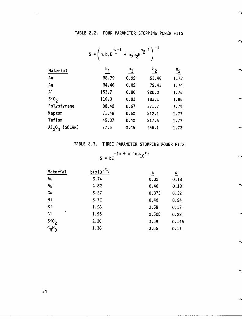
TABLE 2.2. FOUR PARAMETER STOPPING POWER FITS
n1-1 n2-1 S = ( "lb1E + "2b2E r1
Material b1 n1 b2 n2 -Au 88.79 0.92 53.48 1. 73 Ag 84.46 0.82 79.43 1. 74 Al 153.7 0.80 220.0 1. 76 S;02 116.3 0.81 183.1 1.86 Polystyrene 88.42 0.67 371. 7 1. 79 Kapton 71.48 0.60 312.1 1.77 Teflon 45.37 0.40 217.6 1.77 A1 203 (SOLAR) 77.5 0.45 156.1 1. 73
TABLE 2.3. THREE PARAMETER STOPPING POWER FITS
S = bE - (a + clog lOE )
Material b(x10-3) a c - -Au 5.74 0.32 0.18 Ag 4.82 0.40 0.18 Cu 5.27 0.375 0.32 Ni 5.72 0.40 0.24 Si 1.98 0.58 0.17 Al 1.96 0.525 0.22 S;02 2.30 0.59 0.145
C8H8 1.38 0.66 0.11
34

TABLE 2.4. COMPARISON OF THRE~ffD FOUR PARAMETER FITS WITH ATAR
53 = bE -(a + c lO91OE)
-1 (nCI n2-1 ) S4 = n1B1E + n2B2E
Units of S = eV A-I
1. GOLD E SATAR S4 S3 - --
0.1 7.94 8.66 7.92 0.2 8.20 8.23 7.85 0.3 7.79 7.79 7.53 0.5 7.01 7.04 6.90 1.0 5.74 5.74 5.74 2.0 4.37 4.33 4.43 3.0 3.75 3.56 3.68 5.0 2.84 2.69 2.80
10.0 1. 75 1.77 1.82 50.0 0.60 0.60 0.50
2. SILVER E 5ATAR S4 53 - --
0.1 7.04 7.69 8.00 0.2 7.20 7.43 7.49 0.3 6.91 7.00 6.97 0.5 6.27 6.20 6.13 1.0 4.82 4.82 4.82 2.0 3.44 3.42 3.51 3.0 2.80 2.71 2.83 5.0 2.09 1.97 2.07
10.0 1.26 1.24 1.27 50.0 0.39 0.39 0.30
35

TABLE 2.4. COMPARISON OF THREE AND FOUR PARAMETER FITS WITH ATAR (Continued)
3. ALUMINUM E SATAR S4 S3
0.1 4.17 3.81 3.96 0.2 3.56 3.53 3.56 0.3 3.21 3.21 3.21 0.5 2.69 2.70 2.69 1.0 1.96 1.96 1.96 2.0 1.29 1.31 1.30 3.0 0.98 1.01 0.98 5.0 0.69 0.71 0.66
10.0 0.41 0.43 0.35 50.0 0.14 0.13 0.06
4. Si02 --E SATAR S4 S3
-0.1 4.62 5.18 6.41 0.2 4.71 4.69 5.05 0.3 4.20 4.18 4.27 0.5 3.37 3.39 3.36 1.0 2.30 2.30 2.30 2.0 1.48 1.43 1.48 3.0 1.12 1.05 1.11 5.0 0.77 0.70 0.76
10.0 0.46 0.40 0.42 50.0 0.09 0.10 0.09
5. POLYSTYRENE SATAR S4 S3 """ E J
- --0.1 4.24 4.26 4.90 0.2 3.48 3.48 3.53 0.3 2.84 2.90 2.85 0.6 1.91 1.94 1.91 1.0 1.38 1.38 1.38 2.0 0.85 0.84 0.85 4.0 0.50 0.49 0.30 6.0 0.36 0.36 0.36
10.0 0.24 0.24 0.23 50.0 0.07 0.07 0.05
36

TABLE 2.4. COMPARISON OF THREE AND FOUR PARAMETER FITS WITH ATAR (Concluded)
6. KAPTON E 5ATAR 54 S3 - -- -
0.1 4.58 4.96 ** 0.2 4.16 4.14 0.3 3.44 3.47 0.6 2.31 2.35 1.0 1.68 1.68 2.0 1.05 1.03 4.0 0.63 0.61 6.0 0.45 0.45
10.0 0.30 0.31 50.0 * 0.09
* No Bethe data (readily) available. ** No three-parameter fit made.
7. TEFLON E 5ATAR S4 S3 - --
0.1 7.04 7.27 ** 0.2 6.39 6.28 0.3 5.27 5.27 0.6 3.49 3.51 1.0 2.48 2.48 2.0 1.53 1.50 4.0 0.91 0.89 6.0 0.66 0.65
10.0 0.44 0.44 50.0 * 0.13
* No Bethe data (readily) available. ** No three-parameter fit made.
37

TABLE 2.5. COMPARISON OF OLD AND NEW VERSION YIELDS
Old version uses old data, new version, new data. All data refers to a normal, monoenergetic beam.
1. GOLD 0max = 0.88, Emax = 0.8 keV.
E (kev) °old °new 0.1 0.234 0.266 0.2 0.432 0.472 0.3 0.590 0.624 0.5 0.792 0.806 1.0 0.858 0.778 2.0 0.613 0.650 3.0 0.475 0.521 5.0 0.346 0.388
10.0 0.225 0.253 50.0 0.083 0.085
2. SILVER 0max = 1. 000 , Emax = 0.8 keV.
E (kev) °old °new 0.1 0.266 0.289 0.2 0.490 0.518 0.3 0.670 0.692 0.5 0.900 0.908 ""'\ 1.0 0.975 0.937 2.0 0.696 0.692 3.0 0.540 0.532 5.0 0.393 0.379
10.0 0.256 0.236 50.0 0.094 0.075
3. ALUMINUM 0max = 0.970, Emax = 0.3 keV.
E (keV) °old °new --0.1 0.600 0.651 0.2 0.898 0.912 0.3 0.970 0.970 0.5 0.855 0.878 1.0 0.577 0.608 2.0 0.384 0.402 3.0 0.302 0.308 5.0 0.221 0.216
10.0 0.144 0.131 50.0 0.050 0.040
38

TABLE 2.6. COMPARISON OF OLD AND NEW VERSION YIELDS (Concluded)
4. Si02 6max = 2.4, Emax = 0.4 keY.
E (keV) 60ld 6new 0.1 1.094 1.233 0.2 1.875 1.960 0.3 2.287 2.308 0.5 2.325 2.339 1.0 1.507 1.565 2.0 0.887 0.994 3.0 0.662 0.686 5.0 0.462 0.454
10.0 0.285 0.256 50.0 0.094 0.065
5. KAPTON 6max = 2.1, Emax = 0.15 keY.
E (keV) 60ld 6 new 0.1 1.942 1.972 0.2 2.015 2.029 0.3 1.688 1.726 0.5 1.263 1.269 1.0 0.867 0.787 2.0 0.606 0.479 5.0 0.380 0.241
10.0 0.267 0.142 50.0 0.118 0.041
6. TEFLON 6max = 3.0, Emax = 0.3 keY.
E (kev) 60ld 6new 0.1 1. 751 1.971 0.2 2.737 2.798 0.3 3.000 3.000 0.5 2.546 2.615 1.0 1.495 1.514 2.0 0.875 0.889 3.0 0.642 0.650 5.0 0.433 0.439
10.0 0.250 0.257 50.0 0.065 0.075
39
~
) J
'd M Q)
r-I
2.0
:>1 1. 0
<0
----- New Formulat10n
Old Formulation
1 __________ .JL. ____ .l ____ 1. __ L..l __ L.J.J.l. __________ .l ______ 1. __ .l __ .l __ J.-1.J~~~ __________ L. ____ .J __ --~_S~ .. ~ ......... o • 0.1
E (Energy, keV)
Figure 2.3. Comparison of new and old MATCHG yields for kapton.
) ) ,j ) J ) ) ) )

)
~ ......
)
1.0
'tl M Q) 0.5 rl >t
'0
') ) )
----- New Formulation
Old Formulation
o • , , I I I I , ,
0.1 1.0 10.0 100.0
E (Energy, keV)
Figure 2.4. Comparison of new and old MATCHG yields for aluminum.
) )
2.5.3 Ion-Induced Secondary Electron Emission
The NASCAP model assumes that all positively charged species in the plasma environment are protons H+. Measurements made in geosynchronous orbit indicate in fact that often up to 80 percent of
. + + the 10ns present are 0 rather than H. This observation calls into question the ion-impact induced, secondary electron current, calculated by the code assuming a purely proton environment.
Secondary emission of electrons following ion-surface impact can occur via two mechanisms.
a. Potential Emission This occurs via transfer of ion potential energy to lattice electrons at metal surfaces. Electrons tunnel into the potential well formed by the adsorption of the ion on the surface, neutralizing the ion, which then auto-ionizes. It is a low energy phenomenon «20 eV) and is unimportant in most of the energy regime associated with NASCAP (0-50 keY).
b. Kinetic Emission Here emission results from the direct transfer of ion-kinetic energy to lattice electrons, and depends, in a complicated way, on the projectile/target atomic collision cross-section. It is the dominant mechanism in the energy range of interest.
The yield for both mechanisms does not appear to depend in any predictable way upon atomic number. The mechanism for potential emission is almost chemical in nature and depends much more upon electronic structure than nuclear mass. The most identifiable trend appears to be an increasing yield for projectile ions having greater electron affinities.
42
While the collision cross-section central to kinetic emission increases with atomic number of the projectile ion, the yield of escaping secondary electrons involves a trade-off between factors such as the efficiency of energy transfer per collision and the depth of penetration of the ion. This is rather poorly understood and experimental studies with rare gas ions impinging on clean metal surfaces show an irregular dependence of yield upon atomic number. For example, the energy/yield curves for Kr and Xe incident on Mo cross twice within the range 6-10 keY.
A table of secondary yields for ions of 1 keY incident on Mo is shown below.
TABLE 2.6. SECONDARY YIELD FOR 1 keY IONS ON Mo.
Ion Yield (at 1 keY)
H+ 0.250 He+ 0.276 0+ 0.172
In this case the yields for H+ and 0+ are of a similar magnitude. Very little additional data is available. The data that is available is often subject to large errors because of the sensitivity of measurements to the nature of the test surface. This coupled with the fairly large uncertainties in the measurement of O+/H+ ratios in space at any particular time leads us to the conclusion that adjustment of the code and/or data to take the presence of 0+ into account is not justified at this time. The magnitude of the adjustments to be made are smaller than the additional uncertainties that would be introduced.
43

3. NASCAP/GEO EXTENSIONS
3.1 OBJDEF EXTENSION
It is now possible to divide a square cell into two right triangles, either by superseding part of a square cell or by defining two complementary wedges. In particular, it is now possible to supersede a portion of an octagonal surface with a smaller octagon of different material. The extension involved changes to subroutines OBJDEF, WEDGE, CUBE56, NIOWGE, TETRAH, NIOTET, CONDUC, TRNGLS, CMPRSS, SPECEL, DELETE, RECTAN, NIOOBJ, PLATE, and new subroutines NORMSK, RTSUP, WRDSRT, SQUARE. Examples of previously illegal objects are shown in Figures 3.1 and 3.2.
3.2 NEW DISCHARGE CAPABILITY
The NASCAP discharge capability has been revised to be more realistic both as to the triggering configuration and the charge blowoff and redistribution. The old "discharge to space" has been expunged, and a flashover capability added. Reasonable estimates of blowoff of charge to space and to other surfaces have been included. The general principles and specific implementation are presented below.
3.2.1 General Principles Governing Discharges
44
1. A discharge analysis takes place at the end of the LIMCEL routine when DISCHArge d [0 < d ~ 1] has been specified in the RDOPT file.
2. Subroutine DISCHG looks for the "most severe" discharge, with punchthroughs taking priority over flashovers. a. A punchthrough takes place when the potential between
an insulating surface and its underlying conductor exceeds (in absolute value) material property 16. The "severity" is measured by the ratio of differential voltage to discharge threshold.

/ " / '" = = - -
~ v ~ 17
en s:: o Cl ra +l u o
"0 QJ +l en QJ s:: QJ QJ ~
..s:: I-
...... . M
QJ ~ :::I Cl
'r-LL.
45
.L "-L-l.-I..-I..--'--L.-
'-" "-~
46
/1 n
JJ "'" 11 ----~ ~ ~
:7
TT') ~
1
1
tly
· ClJ -c .r-III
to
+oJ to
C'I C
.r-+oJ ClJ ClJ E III I: o C'I to
+oJ U o
~ · N · M
ClJ s... :::l C'I
.r-u..

b. A flashover takes place when two cells sharing a common node differ in potential by more than the flashover threshold, entered in the RDOPT file through the keyword 'FLASHOver volts' {default 10 kV}. Severity is similar to above.
c. After each discharge, charge is redistributed according to the rules below. New potentials are estimated by subroutine VPRED, and DISCHG is called again. The loop repeats, discharging one cell at a time until no further discharge conditions exist.
3. Charge Redistribution - General Rules a. Under "fixed" potential conditions all charge lost by a
negative dielectric is considered "blown off". This charge is immediately and implicitly replaced •
. b. Negligible charge is assumed to flow through a punchthrough, with the exception of punchthrough of a positively charged dielectric, in which case all charge flows through the damage spot.
c. Under floating conditions charge lost by a negative dielectric is immediately blown off to the extent needed to bring the cell near zero potential. Remaining charge is distributed to more positive
-6 cells. This process takes -10 seconds, and typically leaves the satellite well above its "floating potential". Relaxation (typically taking -10-2 seconds) occurs during the next timestep{s}.
47

3.2.2
48
Charge Redistribution - Specific Cases
Symbols: AQ
VC Vold Vnew
Vpt d
Vfl B
CL Cs CTOT
- charge transferred from surface - potential of relevant conductor - cell potential before discharge - cell potential after discharge, calculated
as if conductor fixed - punchthrough threshold potential
- discharge relaxation factor - flashover threshold potential
- blowoff - capacitance, cell to conductor - cell capacitance to tank or plasma ground - object capacitance
a. Punchthrough, negative dielectric, fixed potential
Vnew = Vc - d Vpu
= CL (Vold - Vnew )
B = AQ
b. Punchthrough, negative dielectric, floating potential
Vnew = Vc - d Vpu
AQ = CL ( Vol d - V new)
B = CTOT Vold (Vold < 0)
AQ - B distributed to cells with V > Vnew
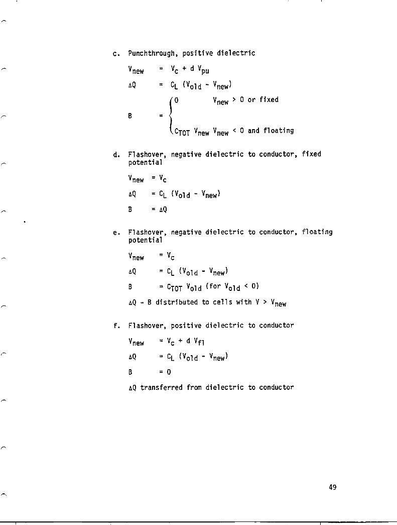
c. Punchthrough, positive dielectric
Vnew = Vc + d Vpu
AQ = CL (Vold - Vnew )
B = {O V
new >
CTOT Vnew Vnew <
o or fixed
o and floating
d. Flashover, negative dielectric to conductor, fixed potenti al
Vnew = Vc
AQ = CL (Vold - Vnew )
B = AQ
e. Flashover, negative dielectric to conductor, floating potenti al
Vnew = VC
AQ = CL (Vold - Vnew )
B = CTOT Vold (for Vold < 0)
AQ - B distributed to cells with V > Vnew
f. Flashover, positive dielectric to conductor
= Vc + d Vfl
= CL (Vold - Vnew )
B = 0
AQ transferred from dielectric to conductor
49
50
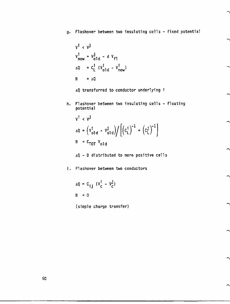
g. Flashover between two insulating cells - fixed potential
Vi < vj
vi = Vj - d Vfl new old
6Q = c[ (V~ld - V~ew)
B = 6Q
6Q transferred to conductor underlying i
h. Flashover between two insulating cells - floating potential
Vi < Vj
.Q = (V~ld - V~ld)/[(C~t + (ctt] B = GrOT Vold
6Q - B distributed to more positive cells
i. Flashover between two conductors
B = 0
(simple charge transfer)

3.3 MULTIPLE TEST TANK ENVIRONMENT
3.3.1 Theory
The existing versions of NASCAP model ground test experiments by using particle pushing techniques to simulate an electron gun. With this method the beam electron trajectories are approximated by calculating the actual trajectories of representative beam particles. While, in principle, enough particles could be followed to make the results as accurate as desired, in practice, computer time used to calculate each representative orbit places severe restrictions on the number of test particles followed. As a result, even for the present single gun, monoenergetic electron beam simulation, the particle pushing was taking upwards of a minute of CPU time per code timestep. The present technique, as implemented, had the added shortcoming of . not correctly accounting for many cases of particle shadowing.
Using particle tracking to determine current density would quickly become unmanageable for a multi-gun, multi-energy simulation. If the present technique were used to simulate five guns of variable energy, it would easily take an hour of CPU time per code timestep. Following the basic philosophy that has been successful throughout NASCAP we opted instead to use a simplified representation of the space potentials which allows direct integration of particle orbit. Particle shadowing is included in an approximate manner using HIDCEL with the "viewer" located at the gun position.
The potential is modeled by keeping only one monopole term in the multipole expansion. This is a reasonable approximation for gun to satellite distance large compared to satellite radius.
To implement the proposed method of approach, consider a point source at a distance ro from the center of force (Figure 3.3). The
rate at which the ~ource emits electrons with kinetic energy Eo into the interval dEo and the solid angle dno is denoted by
51

• x
y
Figure 3.3. Geometry for electron gun aimed at a sphere.
52
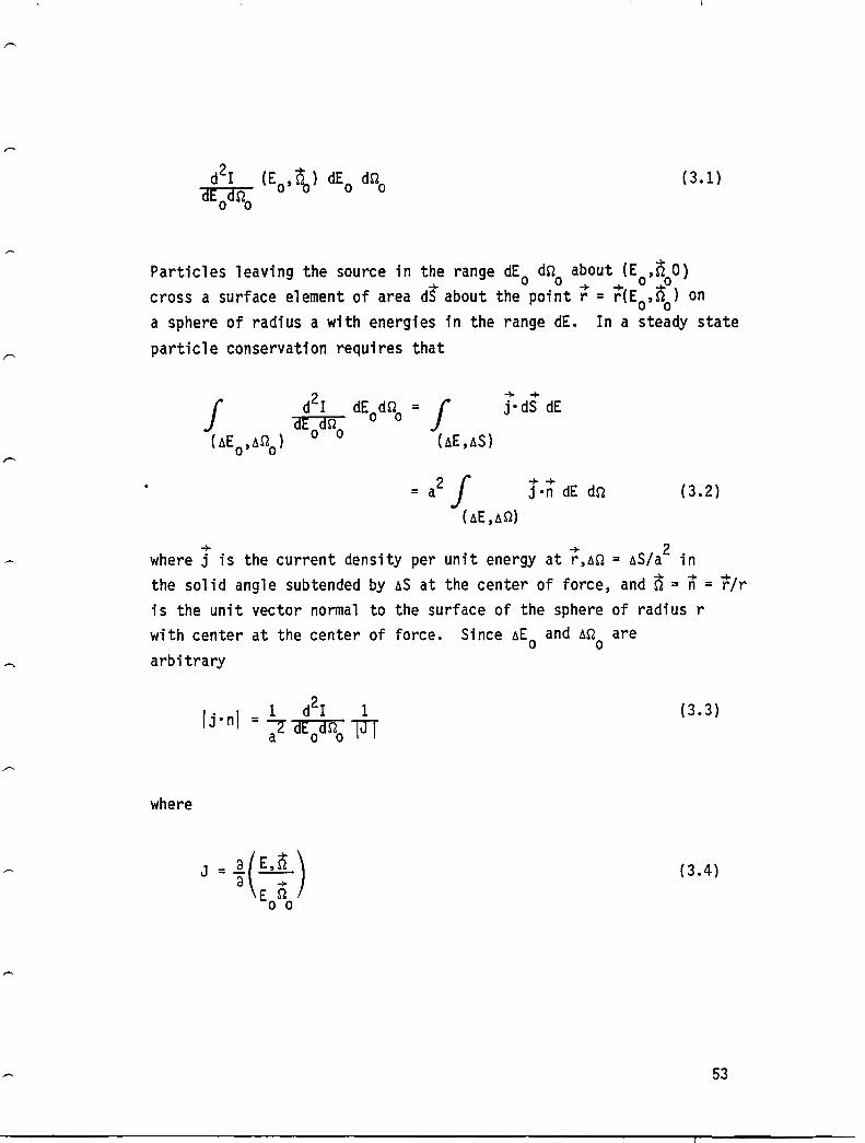
(3.1)
Particles leaving the source in the range dE o dn about (E ,00) ;:t- 0+ +0-jP
cross a surface element of area d~ about the point r = r(Eo'~~) on a sphere of radius a with energies in the range dE. In a steady state particle conservation requires that
+ + j. dS dE
++ j·n dE dn (3.2)
where r is the current density per unit energy at ~,~n = ~S/a2 in the solid angle subtended by ~S at the center of force, and n = n = t/r is the unit vector normal to the surface of the sphere of radius r with center at the center of force. Since ~E and ~n are ° 0 arbitrary
(3.3)
where
(3.4)
53

+ Once Ijenl is determined, the current density j per unit energy foll ows from
+ j = Ijenl_V_ (3.5)
++ Ven
+ The primary problem in the determination of j is the evaluation
of the Jacobian. Consider first the case of no magnetic field and a repulsive potential V = k/r. The particles follow a hyperbolic path with the center of force at the focus. The geometry of the encounter is shown in Figure 3.4 where we also introduce the angular coordinate e in terms of which the orbit is given by[6]
1 r - ~ (1 + £ case) • (3.6)
Here e is measured from the symmetry axis of the orbit, m is the particle mass, i = mvo ro sina = (2mEo)1/2 ro sina is the angular momentum, and
(3.7)
where V = k/r. In the following we shall use the orbit equation o 0
in the form
case 1 (2E
o sin2a ) =-- V- +1
£ \ 0 X (3.8)
with x = r/ro'
54
-
-,

, , , , , , , , , , , , ,
, , "
Figure 3.4. Geometrical quantities used to calculate current density.
55

where
For the present problem the required Jacobian is
J = a (cosx) all
cosx = -cos(e-e ) o
= -(cose coseo + sine sineo)
Il = COSa
and coseo is obtained from Eq. (3.8) with x = 1. We find
J = - 1. [(- 1£ cose + ~.!!.) (cose - sine ctne) e all oX 0 0
+ (- ~~ cos.o + ::0 ,) (cose - sine ctneo)]
with
-+ In the presence of a constant magnetic field, B, spherical
symmetry of the force field is lost and the simple analytic expressions for the particle orbit are not known. The problem simplifies considerably however if the magnetic field is small in a sense that will become clear as we consider the motion observed in a system rotating at a constant angular velocity Z. In the rotating
56
...... .
-,

system the effective force is[7]
where
+ + + V r = V s - wxr
+ + and V and V are the velocities of the particle relative to the s r space and rotating axes respectively. If we choose
+ + 1mc w = - mc
then
+ + + + + Feff = qE + mwx(wxr)
+ Neglecting terms of second and higher order in the B field, the equation of motion in the rotating system becomes
+ dVr +
m dt = qE •
Thus, to the considered degree of approximation, in the rotating frame the effects of the magnetic field vanish and to the rotating observer the particle moves in a l/r potential.
To find where a given particle strikes the body we can consider that during the particle's flight time the body rotates with constant
+ angular velocity -w. The magnitude of the rotation requires a knowledge of the flight time, which to the required order of accuracy
57
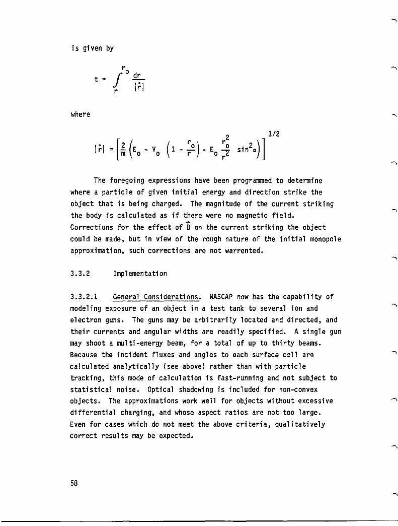
is given by
where
2
1;'1 = [l (E _ V (1 _ r 0 ) - E ~ moo r 0 r~
The foregoing expressions have been programmed to determine where a particle of given initial energy and direction strike the object that is being charged. The magnitude of the current striking the body is calculated as if there were no magnetic field.
+ Corrections for the effect of B on the current striking the object could be made, but in view of the rough nature of the initial monopole approximation, such corrections are not warrented.
3.3.2 Implementation
3.3.2.1 General Considerations. NASCAP now has the capability of modeling exposure of an object in a test tank to several ion and electron guns. The guns may be arbitrarily located and directed, and their currents and angular widths are readily specified. A single gun may shoot a multi-energy beam, for a total of up to thirty beams. Because the incident fluxes and angles to each surface cell are calculated analytically (see above) rather than with particle tracking, this mode of calculation is fast-running and not subject to statistical noise. Optical shadowing is included for non-convex objects. The approximations work well for objects without excessive differential charging, and whose aspect ratios are not too large. Even for cases which do not meet the above criteria, qualitatively correct results may be expected.
58
-...
3.3.2.2 Usage. The new test tank mode operates as flux type (ITYPE) 6. However, because an optical shadowing calculation (for non-convex objects) must be performed for each gun (requiring use of the HIDCEl routines) the flux definition must occur in a special code module, TANK, rather than being called from TRIlIN. Also, this shadowing calculation destroys any previous HIDCEl information, so that the call to HIDCEl must follow the call to TANK (unless I NOSHADOW' is specified). Of course, HIDCEl need not be invoked for simulations having no solar or ultraviolet illumination.
or
Some typical runstreams might be (in part) 1. @USE 22,multiplegundefinitionfile
@XQT NASCAP RDOPT OBJDEF CAPACI TANK TRILIN END
2. @XQT NASCAP RDOPT TANK 5 @ADD multiplegundefinitionfile HIDCEl TRILIN END
59
or 3. @ASG,A prefix19
@USE 19, prefix19
@XQT NASCAP RDOPT TRILIN END
In all the above examples, the specification IITYPE 61 must be included in the options input file. The first example is appropriate to a new run, with an object exposed to particle beams in the dark. The second example allows the possibility of exposure to sunlight or an ultraviolet source. The third example takes advantage of previous storage of the gun shadowing information in file 19.
3.3.2.3 Gun Definition Input Specification. The TANK module consists of two major subroutines, INGUNS and GUNSHD. INGUNS reads user input and writes the gun specifications through subroutine CELLIO. GUNSHD performs a shadowing calculation using the gun location as a viewpoint, and writes the visibility factors on file IOBPLT [19]. If the object has been declared CONVEX, a visibility factor of unity is assigned to each surface cell.
60
The permissible gun definition input cards are:
OFFSET ix ;y iz Should be first card in file. Defines position relative to which gun locations are defined. Default is mesh center. OFFSET 0 0 0 will make gun positions defined in "absolute" grid location.
GUN AT x Y z ELECTRON GUN AT x Y z ION GUN AT x Y z
Defines position and type of gun. If gun type not specified, electron gun is assumed.
ENERGY 1 el ... en unit
ENERGIES f Defines beam energies of gun. Unit is lEVI or IKEVI. The default unit is IKEVI.
BEAMWIDTH(S) bl ... bn unit Defines half-angle of beam. Unit is assumed to be radians, unless IDEGREES I is specified.
ALL BEAMWIDTHS b unit Assigns b as the beamwidth for all beams of this gun.
CURRENT(S) cl ... cn Specifies beam currents in amperes.
ALL CURRENTS c Assign c as current for all beams of this gun.
NOSHADOW Indicates that file IOBPLT [19] already exists for guns at these locations.
ION MASS m unit Defines mass for an· ion gun. Unit is assumed kilograms unless IAMU I is specified.
DIRECTION x y z Specifies direction in \'ihich gun is pointing.
END Ignore subsequent cards.
61

3.3.2.4 Examples. The first example defines four guns pointing at the mesh center, each from a distance of 22.6 grid units. After echoing the gun definition input (which concludes with an IENDI card or end-of-file condition), the gun characteristics are echoed for each gun, and for each beam. It is then indicated that a shadowing calculation is being performed for each gun.
The second example defines an ion gun. As the I NOSHADOW I specification is included, the purpose of this input is presumably to change the beamwidth, current, or energy.
Example 3 defines a two-beam electron gun with different current and beamwidth for each energy. Example 4 defines a three-beam electron gun with equal currents and beamwidths.
62

1-2. 3. I "f.
6. 7. 8. 9.
10. '11. 12. ,13. 14. 15. 16. 17. 18. 19. 20. 21.
1. 2. ., ..,. 4. S. 6. 7. n O.
1-2. 3. I "f.
S. 6.
1. .., ::.. 3. 4. S. 6.
GUN AT 0 'i6 '16 ENERGY 6. ~(EV CURRENT S.E-6 BEAMWIDTH 30 DEGREES DIRECTION 0 -1 -1 GUN AT 0 -~6 16 ENER.GY 6. ~(E'vl CURREN, S.E-6 8EAMWIDTH 30 DEGREES DIRECTION 0 ·i -1 GUN AT 0 -16 -16 ENERGY 6. ~(EV CURRENT S.E-6 BE~MWIDTH 30 DEGREES DIRECTION 0 1 1 GUN AT 0 16 -16 ENERGY 6. ~(EV CURRENT S.E-6 BEAMWIDTH 30 DEGREES DIRECTION 0 - '\ 'I END
Gun definition input for example 1.
ION GUN AT -44., 0.5, 6.2 NOSHADOW ION MASS 'i"f AMU 8EAMUIDTH 20 DEGREES CURRENT S.E-6 ENERGY 5000 El.l DIRECTION 3. O. 1. END
Gun definition input for example 2.
ELECTRON GUN AT -20 O. O. DIRECTION 1 0 0 ENERGIES 0" 1 10 I-{E!) 8EAMWIDTHS 40 10 DEGREES CURRENTS 1.E-6 O.SE-6 END
Gun definition input for example 3.
ELECTRON GUN AT S0 35 4 DIRECTION -2 -1 0 ENERGIES 5 10 20 KEV ALL BEAMWIDTHS 25 DEGREES ALL CURRENTS 1.E-6 END
Gun definition input for example 4.
63

•••••• TU.II 5
OSJECT DEFI~ITIO~ INFORMaTIO~ e~ING READ FROY FILE
A SHADO.ING TABLE wAS PREvIOUSLY GENERATED FOR THIS OBJECT USING THE GUNS OPTION
GUN AT a 16 16 ENERGY 6. KEY CURRENT 5.E-6 aEA~wIDTH 30 DEGREES DIRECTION a -1 -1 GUN AT 0 -16 16 ENERGY 6. KEY CugREhT 5.E-6 BEAMWIDTH 30 DEGREES DIRECTION 0 1 -1
GUN AT a -16 -16 ENERGy 6. KEY CURRENT 5.E-6 BEAMWIDTH 30 DEGREES DIRECTION D 1 1 GUN AT 0 16 -16 ENERGy 6. KEY CURRENT 5.E-6 BEAMWIDTH 30 DEGREES DIRECTION 0 -1 1 END
GUN DEFINITION --~---GUN 1 HAS 6EEh DEFINED _S AN ELECTRON GUN GUN IS LOCATED AT GRID COORDINATES 9.CO 25.00 25.00 GUN DIRECTION IS .00 -1.00 -l.~O BEAM 1: ENERGY: 6.OO+~03 Ev CURRENT: 5.~C-OC6 AMPS
GUN DEFINITION ------GUN 2 HAS SEEN DEFINED AS A~ ELECTRON GUN GUN IS LOCaTED AT GRID COORDINATES 9.00 -7.00 25.00 GUN DIRECTION IS .CC 1.~O -l.~O BEAM 1: EhERGY: 6.:O.C~3 Ev CURRENT: S.JC-C06 AMPS
GUN DEFINITION ------GUN 3 HAS 8EE~ DEFINED AS AN ELECTRON GUN GUN IS LOCATED AT GRID COOROI~ATES 9.00 -7.0e -7.CD GUN DIRECTION IS .00 1.00 1.00 BEAM 1: ENERGY: 6.00+003 Ev CURRENT: S.~0-~06 AMPS
GUh DEFINITION ------GUN ~ HAS bEEN DEFINED AS AN ELECTRON GUN GUN IS LOCaTED AT GRID COORDINATES 9.00 25.00 -7.CO GUN DIRECTION IS .OC -l.OC 1.CO BEAM 1: ENERGY: 6.00.003 Ev CURPENT: 5.~0-C06 AMPS SHADO.ING BEING CALCULATED FOR GUN l
DISTANCE EOUALS 22.627~17
FINAL NAl : 2C SHADOWING BEING CALCULATEu FOR GUN Z
DISTANCE EQUALS 22.627417
FINAL NAI : 20 SHADO,;ING eEING CALCULATED FOR GUN 3 DISTA~CE EOUALS 22.627417
FINAL NA 1 : 2C SHADOIoiING 6E:I~G CALCULATEu FOR GUN ..
DISTANCE EQUALS 22.027 417
FINAL NAl: 2C
CUT-OFF A~GLE: 3D.CCCC DEGREES
CUT-OFF A~GLE: 30.~COO DEGREES
cuT-OFF ANGLE: 3C.O~OC DEGREES
CUT-OFF ANGLE: 30.CCOO DEGREES
Gun definition (INGUNS and GUNSHD) output for example 1.
64
-,

.-
•••••• TANK 5 ION GUN AT -~~., 0.5, 6.2 NOSHADOw ION MASS 111 AMU BEAM~IDTH 20 DEGPEES CuRRENT 5.E-6 ENERGY scao EV DIRECTION 3. o. 1. END
GUN DEfINITION ------GUN 1 HAS BEEN DEFINED AS AN ION GUN _ITH AN ION ~ASS: 2.311-~Z~ KILOGRA~S. GUN IS LOCATED AT GRID COORDINATES -3S.CC 9.5C IS.20 GUN DIRECTION IS 3.00 .00 1.00 BEAM 1: ENERGY: 5.00+003 EV CURRENT: 5.00-Cu6 AMPS CUT-OFF ANGLE: 2~.uOj~ DEGREES
Gun definition (INGUNS and GUNSHD) output for example 2 •
•••••• TANK 5 E~ECTRON GUN AT -ZO c. o. DIRECTION 1 0 0 ENERGIES C.1 10 KEv BEAMWIDTHS 110 10 DEGREES CURRENTS 1.£-6 0.5E-6 END
GUN DEF INITION GUN 1 HAS BEEN DEFINED AS A~ E~ECTRON GUN GuN IS LOCATED AT GRID COORDINATES -11.D~ GUN OIRECTION IS 1.00 .oe .00
9.00 9.00
BEAM 1: ENERGY: 1.CQ+COZ EV CURRENT: BEA~ Z: ENERGY: 1.00+0011 EV CUR~ENT:
... 00-C;:;6 AMPS 5.ao-ee7 AMPS
CUT-OfF ANGLE: u~.ocoe DEGREES CUT-OFF ANGLE: 1:.C~:C DEGREeS
SHADO.ING BEING CALCULATED FOR GUN 1 DISTANCE EQUALS Z:.OOCOOO
fINAL NAl: 16
Gun definition (INGUNS and GUNSHD) output for example 3 .
•••••• TANI'. 5 ELECTRON GUN AT 50 35 II OIPECTION -Z -1 C ENERGIES 5 10 ZO KEV ALL BEJM~IDTHS Z5 OEGREES ALL CURRENTS 1.E-6 ENO
GUN DEFINITION ------GUN 1 HAS BEEN DEFINED AS AN ELECTRON GUN GUN IS LOCATED AT GRID COORDINATES 59.0C GUN OIRECTION IS -~.oo -1.00 .00 BEAH 1: ENERGY: 5.Cj+CC3 EV CURPENT: BEAM Z: ENERGy: 1.00+DOII EV CURRENT: BEAM 3: ENERGy: Z.OD+C~II EV CURPENT: SHADO.ING BEING CALCULATED FOR GUN 1
DISTANCE EQUALS ~1.163713
FINAL NA1: ze
II~.OC 13.0C
.... :;0-(:;:)6 AMPS 1.CO-C06 jMPS 1 ... 0-006 j"P~
CUT-OFF Ar.GLE cUT-orF ANGLE CuT-OFF ANGLE
Gun definition (INGUNS and GUNSHD) output for example 4.
:!s.acc.o OEGI\E S 25.t.::::'C' DEGRE S 2S.~=O::' DEGRE S
65

3.3.3 Cylindrical Tank
The Cylindrical Tank option has now been implemented in NASCAP. This mode is invoked by the option file input cards
TANK RADIUS x [METERS] TANK AXIS a
where ~ is lXI, lVI, or IZI. The default tank axis is Z. If the word I METERS I is omitted, x is assumed given in inner grid units; if I METERS I is specified, the value is immediately converted to grid units using the current value of XMESH. The default tank radius is 'NOPE'.
When the cylindrical tank is requested, the RDOPT subroutine sets IOUTER = 0 and POTSCL = 'NOSCALE'. This is needed because the total charge {found by QSUMER} will not be correct, as the electric . field will be integrated only over the end walls of the tank. On contour plots, the tank wall is drawn as a double blue circle for cuts normal to the axis, and as two sets of double blue lines for cuts parallel to the tank axis. (See Figures 3.5-3.6.)
Examples TANK RADIUS 12. TANK AXIS Z
Defines a tank with radius 12 inner grid units about Z-axis. XMESH 0.3 TANK RADIUS 5 METERS TANK AXIS V
Defines a tank with radius 16.7 grid units about V-axis.
66

POTENTIRL CONTOURS ALONG TH~ X-! PLANE or z - 17
ZMIN - -3.6807+003 ZMRX - .0000
25+ crc~ 6 TIME - 6.08+001
23
21
IS
IS
13
11
9
3
-3
-5
OZ - 2.0000+002
-7 -5 -3 -1 1 3 5 7 9 11 13 is 17 19 21 23 25 '( AXIS
Figure 3.5. Potential contours - cylindrical tank of radius 10 grid units about Z-axis.
67

68
In ;( a: N
POTENTIRL CONTOURS ALONG THE Y-Z PLANE or x - 9
ZMIN - -3 680i+Q03 ZMRX- 0000 OZ - 2.0000+002
i9· CYCLE 6 TIME - 6.08+001
is
i1
37
33
29
25
21
17
13
9
5
-3
-7
-11
-15 • • • + • + • + + • • . . -7 -5 -3 -1 1 3 5 7 9 11 13 IS 17 1921 2325
Y AXIS
Figure 3.6. Potential contours - cylindrical tank of radius 10 grid units about Z-axis.

3.4 SPACE ENVIRONMENT
3.4.1 Anisotropic Flux
The NASCAP model formerly allowed only for incident electron and ion fluxes that are isotropic; i.e., all incident directions are considered equally likely. This is not usually true for orbiting satellites.
Injection of a charged particle into a static magnetic field causes the particle to follow a spiraling trajectory about the
+ magnetic lines of force. The component of its velocity vI I along the field direction is unchanged and the radius of the spiral trajectory rL depends on the perpendicular component vi
Thus for a fixed velocity magnitude, lvi, injection of a flux of charged particles into a magnetic field will lead to fast moving particles (in the field direction) with small Larmor radii (rL), and slower particles with large radii.
Similar events occur in the earth's magnetic field. Plasma is injected into normally low-density regions and the particles begin an orbiting trajectory along the field lines. A satellite bathed in this orbiting plasma will experience a flux with two principal components:
a. A background, essentially isotropic, flux consisting of the pre-existing low density plasma, and particles from the injected plasma, that have rL much greater than the spacecraft's dimensions.
69

b. A directional flux, aligned with the terrestrial field, consisting of particles with rL smaller than the spacecraft dimensions. This can be a negative contribution. If some of the injected plasma has passed the poles several times, the faster moving particles will have been "filtered out" leaving a reduced flux in the field direction (a "loss-cone").
This model is too simplistic to account for all of the varied magnetic phenomena that can occur in earth orbit. However, it does illustrate the features that are desirable in a model incorporating anisotropic flux distribution.
The form introduced into the NASCAP model consists of a background isotropic component and a cos2e distribution aligned with the field direction. The shape of such a form depends on just one parameter: the ratio of integrated flux for each component, R.
3.4.1.1 The Coordinate System. The most convenient coordinate system in which to represent the aligned component is the "fan"-like system shown in Figure 3.7. The angle of incidence s of an incoming vector; is related to the two angles of rotation shown, e and D, by the relationship
coss = cose cos~
Rotating the "fan" from a plane containing the surface normal to a plane containing the vector r only partially defines the angle e. The choice of e becomes unique when the second rotation (6) within the
+ plane of the "fan", to reach r, is specified. The coordinate system +
is chosen so that the magnetic field direction B has D = O. This provides a reference point for all other vectors in the space above the surface, and hence fully defines the e, 6 coordinate system.
70
-
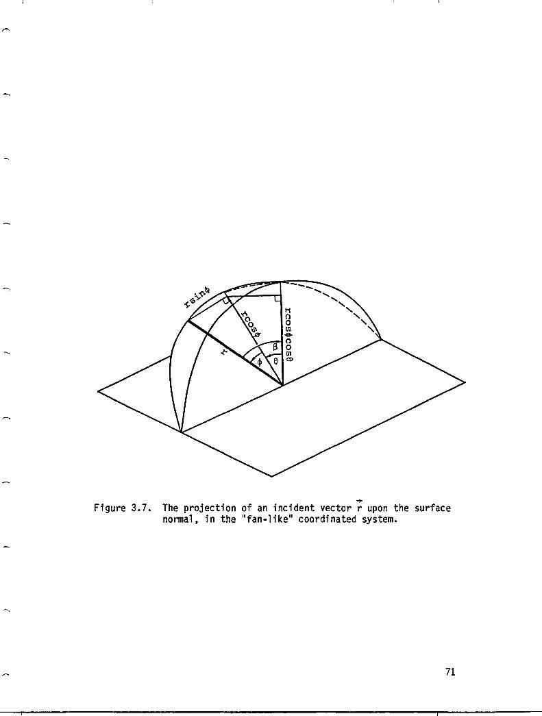
-+-Figure 3.7. The projection of an incident vector r upon the surface
nonnal, in the IIfan-l ike ll coordi nated system.
71

3.4.1.2 Angular Distribution Function. The angular distribution function is assumed to be symmetric about the field direction, and so the aligned component depends only upon the angle ~ made between a
-+ -+ vector rand B, the field direction
cos~ = cos(e-eo) cos~
The form we choose for the aligned component is simply cos2~, i.e., the angular distribution function f(e,~) becomes
2 2 f(e,~) = a + b cos (e-eo) cos ~
Integration over the half-sphere must be normalized to 2~.
~ f(e,~)dw = 2~ 1/2
In the II fan II coordinate system:
dw = cos~ d~ de
~/2 ~/2
~ ~ (a + b cos2(e-eo) cos2~) cos~ de d~ = 2~ -~/2 -~/2
2~a + ¥ = 2~
i . e. ,
72
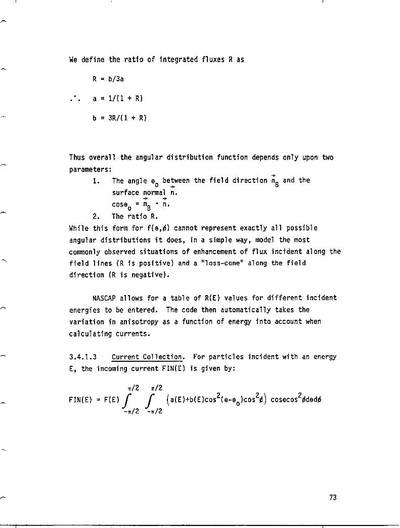
We define the ratio of integrated fluxes R as
R = b/3a
a = 1/(1 + R)
b = 3R/(1 + R)
Thus overall the angular distribution function depends only upon two
+ parameters:
1. The angle eo be~ween the field direction nB and the surface normal n.
+ + coseo = nB • n.
2. The ratio R. While this form for f(e,~) cannot represent exactly all possible angular distributions it does, in a simple way, model the most commonly observed situations of enhancement of flux incident along the field lines (R is positive) and a "loss-cone" along the field direction (R is negative).
NASCAP allows for a table of R(E) values for different incident energies to be entered. The code then automatically takes the variation in anisotropy as a function of energy into account when calculating currents.
3.4.1.3 Current Collection. For particles incident with an energy E, the incoming current FIN(E) is given by:
v/2
FIN(E) = F(E) ~ -v/2
v/2
~ (a(E)+b(E)cos2(e-eo)cos2~) cosecos2~ded~ -v/2
73
where for a Maxwellian
1/2 F ( E) =!! ( T) e -E /T
v 2vm
Integrating gives
[ 3b(E) ( COS2eo )] FIN(E) = F(E) aCE) + --s-- 1 + 3
Integrating over the plasma energy spectrum gives the observed incident current FIN. The emitted current is more complex since all of the integrals cannot be performed analytically.
v/2 v/2
FOUTCEl = F~El f f ,CsHEl [aCEl+bCElCOS2CO-OolCOS26] -v/2 -v/2
= 2 F(E) A(E) ~Iso(E) + K(E)
For secondary electron emission, expanding cos2(e-eo) cos2~:
C2 ( 3 -Q ( 3 3) 1 ) ] + Q2 Q2 - e 1 + Q + Q2 - 2'
74

'--...
where
_ [( 1_e-QCOSS) (1_Coss+l)e-QCOSS)] <5 ( s) - C e C1 Qcoss - C2 2 2
Q cos s
Q = aR (R is the range of electrons of energy E).
K2(E) = sin2eo F~E) beE) C[C1 e I1 + C2eI2]
The integrals 11 and 12 are integrated numerically and tabulated for various values of Q. Interpolation finds the value of each for an unknown Q.
v/2 v/2 _Q
11 = f f (.!:t- )cos4
gS cose de d,s -v/2 -v/2
v/2 ./2 _Q) 12 = f ~ (l+(Q+~)e cos4
gS cose de d,s
-v/2 -v/2 Q
By dividing the values of FOUT(E) so calculated by the incident current normalization ANGF(E)
ANGF(E) = FIN(E) = aCE) + ~ F(E) 0
we obtain the anisotropic yield for secondary emission
FOUT(E) <5ANISO = ANGF(E)
75
The proton secondary emission is much simpler to calculate since FOUT(E} is independent of angle:
oproton(E} _ FOUT(E} FOUT1SO(E} ANISO - ANGF(E) = ANGF(E)
The backscatter requires an additional tabulated integral:
where
where
-logno logno cosa nee} = nee o
F(E} -logn (E) FOUT(E) = -- TI (E) e 0 K
~ 0 n
~/2
f -~/2
Separating as before:
~/2 f e ycosecos~ cos4~ case de d,s
-~/2
J2 is tabulated for values of Tlo.
76
-

3.4.1.4 Fitting Data. Values for R(E) are obtained by fitting the observed distribution function data as a function of pitch angle, W, to the form
_ [1 3R cos2w ] f(w) - N (l+R) + (1+R)
where N is the value of the distribution function close to a pitch angle of 90 degrees.
Some examples of f(~) are shown in Figures 3.8-3.12 for different values of R. The figures show a cross-section through the full three-dimensional distribution function, obtained by rotation about the field direction axis.
As R increases from -0.35 to 0.5 from Figure 3.8 to Figure 3.12 the distribution changes from the IIdoughnutll shaped loss-cone form to a IIdumb-bell ll aligned flux form. Figure 3.10 corresponds to the isotropic spherical distribution.
In conclusion, this simple one parameter representation is flexible enough to provide an adequate model for the angular distributions of electron and ion fluxes found in earth orbit. In addition, it is simple enough to be included in the NASCAP numerical model without decreasing its speed or increasing its size to unmanageable levels.
77

)
....... 00
) J
-2.0
ANGULAR DISTRIBUTION (H) AND a
" ::
~
a -I
ftNISOTRlPlC n.UX HITH R-::~ -.35 I
'" r}
fIT fOR ELECTRONS
2.0
Figure 3.8. Anisotropic flux distribution with R = -0.35.
) .) ) ) ) ) ) )

-...,J \.0
) ) )
ANGULAR DISTRIBUTION (H) AND
~
~
~
ID o
.. o
Z" 8 0
ti 0:::0
-1.21 -1.0 -0.8 -0.8 -0.. -0·.2 c "0 0.2 0 .•
d" i:1ji
.. Iji
.., Iji
~ ANISOTROPIC flUX HITH R- I -.10
"! i
~ I
)
fIT fOR ELECTRONS
1.2
Figure 3.9. Anisotropic flux distribution with R = -0.10.
)

co o
)
--.0
)
ANGULAR DISTRIBUTION (K) AND fiT fOR ELECTRONS
.. d
.. d
... d
... z· CO .... ~ 0::0 ~
-0.1 -0 •• -o.t -0.3 0 ~D 0.3 0 •• D.S 0.' o
d ....... 1&.' ?
... ?
.. ?
OTROPIC flUX HITH R-.. I .00 ?
~
Figure 3.10. Isotropic flux distribution.
) ) ) ) ) ) ) )
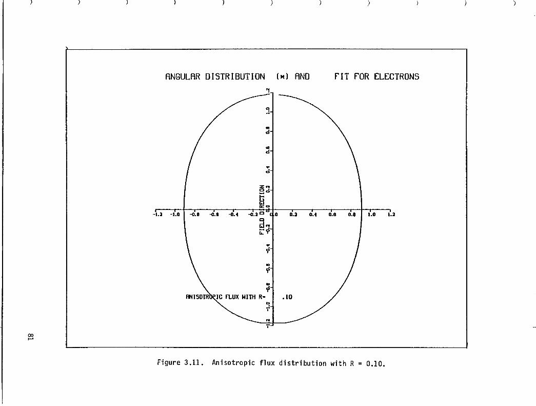
(» .....
) )
ANGULAR DISTRIBUTION (H) AND ~
z ... o· .... 0
ti 0::0
)
rlT fOR ELECTRONS
-1.:2 -1.0 I -0.8 -0.' -0.. -0.3 c .. ~O 0.3 0.. 0.8 0.' I 1.0 1.3
d ... [:~
.. r? .., r?
9 i
... i
.10
Figure 3.11. Anisotropic flux distribution with R = 0.10.
)

)
co N
) )
ANGULAR DISTRIBUTION (H) AND fIT fOR ELECTRONS a ~
-:1.0 -1.5 -1.0 1.0 1.5 :1.0
a ~
Figure 3.12. Anisotropic flux distribution with R = 0.50.
) J ) ) ) ) ) )

3.4.2 DIRECT and UPDATE
The model for the description of the plasma surrounding the spacecraft in NASCAP has been extended. Now, in addition to isotropic Maxwellian and double Maxwellian representations, tabulations of distribution function data, as observed experimentally, may be entered directly. The angular distribution function may also be entered, as a function of energy, for each species (electrons and ions).
In addition, as an aid to simulation of charging events over a period of time where several measurements of the environmental parameters are available, the UPDATE feature has been added. In this mode NASCAP continually updates the environment description to correspond to the latest available.
3.4.2.1 DIRECT. The direct input of a tabulation of distribution function data points has been added as a new flux definition type 5. It may be invoked with a flux definition card in the FLX file of the type 'ITYPE 5', or 'DIRECT'. Following this, three cards specifying 'YEAR', 'DAY', 'TIME' must be included to pinpoint the data set to be used; e.g.,
YEAR 1980. DAY 87. TIME 59630.
The order of the cards is unimportant. All values are real. The time is in seconds. Syntaxes are given in Table 3.1 and examples in Figure 3.13. The data itself must be in the standard format described in Section 3.4.3, and resides in a separate file ISPCTR. The default value of ISPCTR is 9.
83

)
(X) -1=:0
)
TABLE 3.1. SYNTAX
a. Flux File Cards (or ISPCTR)
Syntax
01 RECT (ITYPE 5)
YEAR <year>
DAY <day>
TIME <time>
ANISOTROPIC <ianiso>
<energy unit> <energy> ERATIO <ratio>
<energy unit> <energy> IRATIO <ratio>
b. Option File
Meaning
Flux type 5, direct input of data from ISPCTR
YEAR associated with data to be read under DIRECT
DAY associated with data to be read under DIRECT
TIME in seconds on day associated with data to be read under DIRECT
Read RATIO cards from unit IANISO and use ANISOTROPIC mode
Value of ratio, R, for electrons of energy given
Value of ratio, R, for ions of energy given
Syntax Meaning Defaul t
UPDATE ON Read flux data from ISPCTR and update where possible OFF
UPDATE OFF Read flux data from FLX. file in the normal way OFF
ISPCTR <lspctr> Specify the unit for DIRECT mode - or the UPDATE file 9
) ) ) ) ) )
Exampl e
DIRECT
YEAR 1980.
DAY 146.
TIME 15216.
ANISOTROPIC 19
KEV 10. ERATIO 0.8
EV 1000. IRATIO - 0.2
)
Exampl e
UPDATE ON
UPDATE OFF
ISPCTR 11
) )

co 01
)
a.
)
UPDATE OFF. ISPCTR = 9.
Fil e 22
DIRECT
TIME 59001
DAY 87
YEAR 1979
ANISOTROPIC 25
END
Fll e 25
KEV 0.1 ERATIO 0.9
KEV 0.5 ERATIO 0.5
KEV 2.0 ERATIO -0.2
KEV 10.0 ERATIO -0.01
KEV 50.0 ERATIO 0.0
EV 1000 IRATIO -0.2
EV 3000 IRATIO -0.05
EV 40000 IRATIO 0.06
END
) ) )
b. UPDATE ON. ISPCTR = 9.
Fil e 22
DOUBLE MAXWELLIAN
TIME 59050
END
File 9
TIME 59000
ELECTRONS 0.3E6 MKS 10 KEV
ELECTRONS 0.7 CGS 500 EV
PROTONS
PROTONS
END
TIME 59100
0.3 CGS 1.E6 KELVIN
0.7 E6 MKS I.E-IS JOULES
ELECTRONS etc.
etc.
)
For an example of file 9 see Section 3.4.3.
Figure 3.13. File examples for DETECT and ANISOTROPIC fluxes.
)
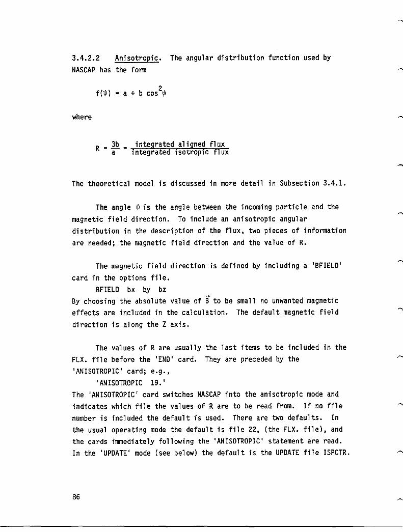
3.4.2.2 Anisotropic. The angular distribution function used by NASCAP has the form
where
2 f(W) = a + b cos W
= 3b = integrated aligned flux R a integrated isotropic flux
The theoretical model is discussed in more detail in Subsection 3.4.1.
The angle W is the angle between the incoming particle and the magnetic field direction. To include an anisotropic angular distribution in the description of the flux, two pieces of information are needed; the magnetic field direction and the value of R.
The magnetic field direction is defined by including a 'BFIElD' card in the options file.
BFIElD bx by bz ~
By choosing the absolute value of B to be small no unwanted magnetic effects are included in the calculation. The default magnetic field direction is along the Z axis.
The values of R are usually the last items to be included in the FlX. file before the 'END' card. They are preceded by the 'ANISOTROPIC' card; e.g.,
'ANISOTROPIC 19.' The 'ANISOTROPIC' card switches NASCAP into the anisotropic mode and indicates which file the values of R are to be read from. If no file number is included the default is used. There are two defaults. In the usual operating mode the default is file 22, (the FlX. file), and the cards immediately following the 'ANISOTROPIC' statement are read. In the 'UPDATE' mode (see below) the default is the UPDATE file ISPCTR.
86

The cards defining the ratio R, whether following in the FLX. file, or in a separate file, must have the format
<energy unit> <energy> ERATIO <R>
e.g., for electrons 'KEV 1. ERATIO 0.5 1
and for ions
or IRATIO
'JOULES 9000. IRATIO - 0.21 The energy units allowed are keY, eV, joules, ergs, kelvin.
If more than one card is included for one species, NASCAP linearly interpolates the value of R between the energies when necessary. The values at zero and infinity are taken as the values for the lowest and highest energies known, respectively. A maximum of ten cards per species can be read. Syntaxes and examples are given in Table 3.1 and Figure 3.13.
3.4.2.3 UPDATE. I UPDATE I is a new keyword that may appear in the options file.
'UPDATE ON ' 'UPDATE OFF '
The default is 'OFF ' , when the code behaves as it always has.
When I UPDATE I is 'ON ' the flux is read from a new file ISPCTR. (The default value for this is 9.) The code searches ISPCTR for the most recent spectrum and updijtes the flux description correspondingly. For example, suppose a 60 second time step began at time 59803 seconds, the next time step begins at 59863. If ISPCTR contains data for times 59800 and 59850, then for the second time step, UPDATE will change the environment description from that measured at 59800 to 59850. UPDATE always looks backwards to the most "recent" data.
87
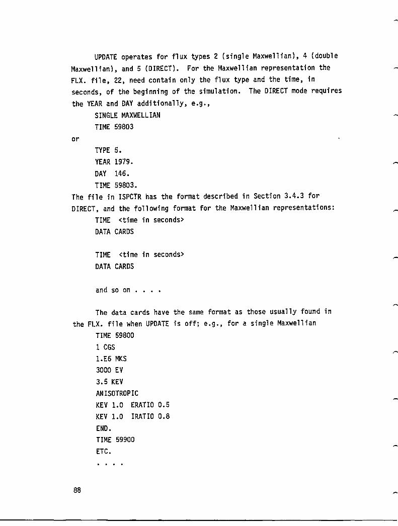
UPDATE operates for flux types 2 (single Maxwellian), 4 (double Maxwellian), and 5 (DIRECT). For the Maxwellian representation the FLX. file, 22, need contain only the flux type and the time, in seconds, of the beginning of the simulation. The DIRECT mode requires the YEAR and DAY additionally, e.g.,
or
SINGLE MAXWELLIAN TIME 59803
TYPE 5. YEAR 1979.
DAY 146.
TIME 59803. The file in ISPCTR has the format described in Section 3.4.3 for DIRECT, and the following format for the Maxwellian representations:
TIME <time in seconds> DATA CARDS
TIME <time in seconds> DATA CARDS
and so on .
The data cards have the same format as those usually found in the FLX. file when UPDATE is off; e.g., for a single Maxwellian
TIME 59800
88
1 CGS 1.E6 MKS
3000 EV 3.5 KEV ANISOTROPIC KEV 1.0 ERATIO 0.5 KEV 1.0 IRATIO 0.8
END. TIME 59900
ETC.

As shown in the above example, the angular distribution function of the flux can also be included in the update file just as in the FLX. file. The exception to this is the DIRECT mode: ANISOTROPIC and DIRECT cannot be used together in the UPDATE mode. The reason for this is that inserting RATIO cards in the files, carefully prepared according to the format shown in Section 3.4.3, would cause confusion and difficulty in reading the data in other operating modes.
3.4.2.4 Summary.
1. Direct input of spectral data points into NASCAP is now possible using ITYPE 5, the 'DIRECT ' flux type.
2. The angular distribution function of flux types 'SINGLE MAXWELLIAN I , 'DOUBLE MAXWELLIAN I , and 'DIRECT ' may be specified using the 'ANISOTROPIC ' statement in the flux file.
3. Simulations over many timesteps, during a period when several characterizations of the environment are available, are made easier by the use of the UPDATE option. In this mode the code automatically changes the environmental description when appropriate, using data compiled in file ISPCTR. UPDATE may be used for flux types 'SINGLE MAXWELLIAN I , 'DOUBLE MAXWELLIAN I , and 'DIRECT'.
89
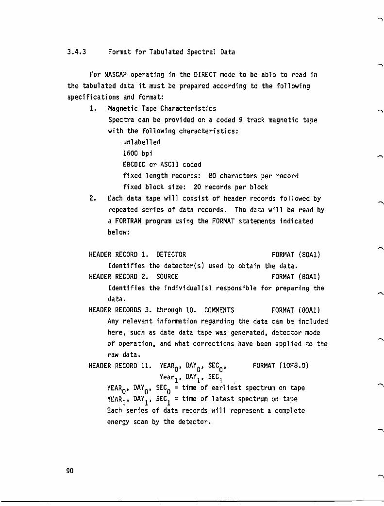
3.4.3 Format for Tabulated Spectral Data
For NASCAP operating in the DIRECT mode to be able to read in the tabulated data it must be prepared according to the following specifications and format:
90
1. Magnetic Tape Characteristics Spectra can be provided on a coded 9 track magnetic tape with the following characteristics:
unlabelled 1600 bpi EBCDIC or ASCII coded fixed length records: BO characters per record fixed block size: 20 records per block
2. Each data tape will consist of header records followed by repeated series of data records. The data will be read by a FORTRAN program using the FORMAT statements indicated below:
HEADER RECORD 1. DETECTOR FORMAT {BOAl} Identifies the detector{s} used to obtain the data.
HEADER RECORD 2. SOURCE FORMAT {BOAl} Identifies the individual(s) responsible for preparing the data.
HEADER RECORDS 3. through 10. COMMENTS FORMAT {BOAl} Any relevant information regarding the data can be included here, such as date data tape was generated, detector mode of operation, and what corrections have been applied to the raw data.
HEADER RECORD 11. YEARO' DAYO' SECO' FORMAT {IOFB.O} Year!, DAY!, SEC! ,
YEARO' DAYO' SECO = time of earliest spectrum on tape YEARl , DAYl , SEC! = time of latest spectrum on tape Each series of data records will represent a complete energy scan by the detector.

+ DATA RECORD 1. YEAR, DAY, SEC, NBINS, DELTA, VSAT, lSI,
SX, XY, SZ FORMAT (10F8.0) YEAR, DAY, SEC = time energy scan was begun NBINS = number of distinct energy bins in the scan DELTA = time (seconds) between each data point in the scan
of the spectrum VSAT = satellite potential during scan (volts) lsi = sun intensity (1.0 = full sun) SX, SY, sz = normalized sun direction vector components
at start of scan DATA RECORDS 2. through (NBINS+1). ENERGY, lo910(Fi ),
l0910(Fe, n, a, BX, BY, BZ FORMAT (10F8.0) Each of these records represents a data point on the scan of the energy range ENERGY = energy (eV) F. = ion distribution function (sec3/m6) Fl = electron distribuition function (sec3/m6) e
n = detector view angle (degrees) a = pitch angle (degrees) BX, BY, BZ = magnetic field vector components
-9 2 (nT = 10 W/m) (The a value is redundant since it can be calculated from n and the magnetic field vector.)
DATA RECORD NBINS+2. (END OF DATA MARKER) FORMAT (10F8.0) This record will contain any negative indicate the end of the spectral scan. redundant since NBINS is known.)
real number to (This record is
The data records 1 through (NBINS+2) are then repeated for each spectrum. Some of the information above may not be available for each spectrum or each data point. The following conventions can be used to indicate that the data is to be ignored:
91
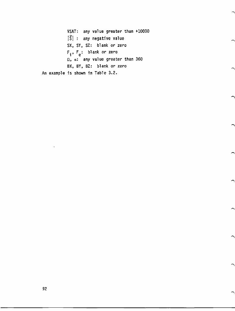
VSAT: any value greater than +10000
I~I any negative value SY, SZ: blank or zero F: blank or zero e
n, a: any value greater than 360 BX, BY, BZ: blank or zero
An example is shown in Table 3.2.
92

I npl
TABLE 3.2. EXAMPLE OF A DIRECT DATA FILE 1:0ETECTOR}NORTH/SOUTH ON SC-9 2:S0URCE }J. DAV!D NICHOLSI UC~O 3:COMn8lTS}BACKGROUNO COUNT SET AT 100 4sCOMMENTS)POTENTIAL EST!MATED ;:MM D!STR~BUTION :OUtl S:COMME)jTS)NO SUN VECTOR OR :.BSOLUTE ATTITUDE INFORM o:COMMENTS>! TRIED TO GIVE MORE CLOSELY ':;PACEl; DATA U"EN 7:COMMENTSlTHE POTJ::NTIAL IS CHANGING MOST R!loPICLY 8:COMMENTS)UE COME OUT OF ECLIPSE ABOUT 17:15 ~ s COMME~lTS >FOR ABOUT 10 MINUTES AFTE'\. TI-lIS ?OTENT!ALS ARE
10:COMME1HSONL,( ROUGH ESTIMATES - HIGHL ( UNCE:RiAIN 11: 1979 87 59400 1979 87 63053 12: '979 87 S9473 04 ').25 O. -1.00 1).00 13: -3.90 0.00 0.00 0.00 96.20 -12.09 -171.27 90.26 14: -1.60 0.00 0.00 0.00 86.50 -11.80 -162.32 108.9S 15: 1.00 0.00 -11.;8 0.00 96.50 -11.S0 -162.32 108.9<; 16: 4.00 0.00 -12.91 0.00 86.50 -1'.90 -162.32 108.~5 q. 7.40 0.00 -1".3" 0.00 'l6.50 -11.90 -162.32 ;08.95 18: 11.40 0.00 -14.a6 0.00 86.ao -11.ao -.49.58 126.12 ~9: 16.00 0.00 -15.20 0.00 86.90 -11.80 -·49.58 126.12' 20: 21.20 0.00 -15.64 0.00 86.80 -11.80 -149.58 126.12 21: 27.20 0.00 -15.82 0.00 96.80 -11.80 -149.58 126.12 22: 34.00 0.00 -15.92 0.00 87.00 -12.09 -134.77 141.54 23: 41.90 0.00 -16.03 0.00 87.00 -12.09 -134.77 441.54 24: 50.90 0.00 -,16.00 0.00 87.00 -12.09 -134.7" 141.5" 25: 61.30 -12.22 -16.08 0.00 87.00 -12.09 -134.77 141.54 26: 73.10 0.00 -16.14 0.00 97.20 -42.09 -118.75 155.79 27: 96.00 -12.52 -1~.16 0.00 87.20 -12.09 -118.75 155.79 28: 102.20 0.00 -16.20 0.00 87.20 -12.09 -118.75 1S~.7° 20: 119.90 0.00 -16.27 0.00 ~7.20 -12.09 -118.75 -5S.7Q
30: '40.30 -12.94 -16.31 0.01) 87.50 -12.09 -100.99 Ib7.95 21: 163 • .:.0 -'12.77 -16.36 0.00 a7.S0 -12.J9 -iOO."'8 '67 .·~5 32: 190.30 -12.48 -16.32 0.00 87.50 -12.09 -AOO.99 '67.95 33: 220.~0 -13.33 -16.35 0.00 37.50 -12.09 -100.99 107."'5 34: 255.90 -12.83 -16.37 0.00 87.70 -12.09 -92.02 17S.04 35: 205.90 -12.96 -'16.43 0.00 37.70 -'12.09 -82.02 17S.0~ 36: 341.ao -13.41 -16.47 0.00 87.70 -12.0'" -82.02 172.04 37: 394.~0 -12.97 -46.S5 0.00 37.70 -12.09 -82.02 179.04 38: 45~.00 -'13.05 -10.59 0.00 97.90 -12.09 -",2.18 ~es.a~ 30: 523.50 -13.~8 -16.70 0.00 87.90 -12.09 -~2.18 ·85.90 ~o: 602.~0 -'13.39 -16.85 0.00 87.90 -12.00 -62.18 1SS.80 ~,: ~92.70 -'3.19 -16.94 0.00 97.90 -12.09 -62.19 ,95.90 ~2: 706.20 -13.4a -17.03 0.00 88.10 -12.09 -41.7~ 10·.4~ 43: 914.60 -13.71 -17.14 0.00 S8.10 -12.09 -41.71 191.44 44: 1050.20 -.3.59 -;7.26 0.00 98.,0 -'2.00 -~4.7' ;0·.~4 45: 1205.50 -13.03 -17.38 0.00 a8.10 -12.09 -41.71 19'.4" 40: 1383:30 -13.S2 -17.50 O.CO a8.30 -42.09 -20.39 105.00 ~7: '~Bo.90 -;3.S3 -17.70 0.00 98.30 -'I2.0~ -20.39 '9~.O~ 48: .820.00 -13.02 -17.89 0.00 a8.30 -12.09 -20.30 'QS.CC 40: 2087.00 -13.51 -18.00 0.00 S8.30 -12.09 -20.~o 195.~0 SO: 2392.60 -A3.03 -18.20 0.00 a8.~0 -'I2.3Q '.05 10~.1° 51' 2742.S0 -13.95 -'S.33 0.00 3adO -12.39 1.)5 '9",. '9 52: 31.3.20 -1 •• 07 -19.38 0.00 a8.40 -'2.39 1.05 19",.10 53: 3602.0') -14.11 -18.90 0.<)0 98.40 -12.30 '.05 -"6.'9 54: 4127.30 -14.01 -19.07 O.CO 98.~O -12.69 22.3~ ·9S.~0 55: ~729.70 -'4.37 -19.32 0.00 38 •• 0 -42.09 12.37 '95.00 So: 5~17.*0 -14.33 -49.74 0.00 aa •• o -12.60 22.37 10~.00 57: .200.00 -14.~0 -19.a5 0.)0 S8.~0 -12.09 22.37 1'5.00 S8: 710a.90 -14.~6 -20.28 0.00 S9.50 -12.99 ~3.~O '9'.44 S9~ 9t42.7o- ---'1'4-.. 55 -20-.7': ---~.oo ~.sV' -'I2.0g- 4:!t ... cr ---9 •• "" ~O: 932o.~O -14.59 -20.97 0.00 98.SC -42.98 42.40 '9'.~-~ l' 10691.70 -44.07 -20.9~ 0.00 39.5.) -12.'8 -3.-0 '''''.-'' b2:':233.60 -14.7? -21.22 0.00 38.50 -13.29 !3.S7 ·SS.S1 ,:;: '4,)<0.50 -14.a9 -2~.24 0.00 '38.50 -13.:9 ~3.a7 '95.:;' 0-: t60~S.OO -15.05 -21.48 0.00 88.50 -13.29 S3.a~ '85.5 ~S:'837~.60 -1S.37 -22.22 0.00 as.so -13.28 63.37 '95.51 ,6:21041.90 -15.34 -21.91 O.~O 68.~O -13.23 93.71 17~.~~ 07:Z4096.'~O -15.49 -21.7S 0.00 '38 ... 0 -13.58 83.71 177 .~ .. 68:27592.90 -15.70 -21.78 0.00 88.40 -.3.58 83.7' 177.4-.9:31596.90 -'5.90 -22.17 0.00 88.40 -'3.S8 83.71 177.44 ~0:36181.50 -1o.VS 0.00 0.00 9S.S0 -13.5a 402.96 '67.05 7':41~30.90 -46.10 -22.88 0.00 98.50 -13.sa '02.96 167.06 ~:~7 .. 41.40 -~6.C2 -2~.30 0.00 aa.50 -13.58 '02. 06 ·S7.0: 73:S~323.40 -16 ... 7 -22.0~ 0.00 '3a.so -·3.5a ·02.?~ 1",7.0e ~4'~2203.30 -16.05 -23.23 0.00 a8.40 -13.37 '2'.48 ,S_.O~ ~S:7;2:;S.3C -17.06 0.00 1.00 ?9.~~ -13.37 20.~~ 15~.?0 70'91550.00 -A7.51 -23.28 0.00 99 ... 0 -13.37 ;20.~8 ,5-.~0 .,.-: --1. -8: ;07';1 -7. -3.~'J
3C: -,.70 '3" , .00 032: ~.OO 33: i 40 a .. : 11. 4 0 ?s: >.00 36: 2'.20 S7' 2- .2, 33: :; .... ,0 ''39, -1.~')
37 0.00 o.co ').',0 0.00 ?OO 0.00 J.OO 0.00 0).00) ).00
- '1.8' ) •• )0
0.0"
59673 0.0·) ').00
-11. ,5 -·2.9", -13.63 -14.~ .. -",*.70, -15.05 -"S.27 -15.55
S4 '.).00 O. ),) ').':0 O.CI) ".)0 ~ .0,,) 1).00 ,J.OO ) ,,0 O.IV ~.))
... ...rV._::J
'0 .... ; "0.:0 "0.30 :0.30 "0.30
~r).2t)
)0.20 2~. ~"
3'.30 3°.50 ~': ;"1
O. ').30
I'. 's 0.1'; ) .95 ".°5
, ,~ .-~
~.9S
-".co '~ ... 2Q ~6~ . .1" ·~;j.~3 ~ ~3 ... 3 '~3 ... '3
-87.55
-"00.;: -~Qe .::::=
i3S.38 -.,1 Q 7: '35.39 -"39.72 '3S.2S -i3".7: ~js.sa -~3? 72
0.00 0.00
'J.OO) "'.JO
93

4. PLOTTING EXTENSIONS - NASCAP*PLOTREAO
The graphics capability has always been one of the most time-consuming problems in NASCAP code maintenance and code installation. Among the repeatedly encountered problems associated with performing graphics directly were (1) significant amounts of core storage devoted to graphics instructions and data; (2) changes in locally implemented graphics software and hardware beyond our control; (2) non-transferability of absolute elements; (4) difficulties in making optimal use of hardware; (5) difficulties in developing and testing interface routines to new graphics packages. The problem became particularly serious with the need to use the OISSPLA package at S-Cubed, as the size of these routines did not permit any hope of including them directly in NASCAP. Thus it became necessary to develop a new graphics protocol for NASCAP.
Under the new protocol, the higher level data manipulation routines (contouring, shading, perspective projection) are considered part of NASCAP. However, lower level routines (draw lines; print letters) are coded in a manner to permit replication of subroutine calls. A list of these routines, together with their functions, is given in Table 4.1. Each routine produces a sequence of words
consisting of: Word 1: Number of words in plot call. Words 2-3: Subroutine name. Subsequent words: Subroutine arguments, as needed.
The key subroutine in this scheme is IGFBUF. IGFBUF maintains a buffer of 280 words, and is called by each pseudo-graphics routine. If the buffer has insufficient storage remaining to store the plot calls the buffer is written out to file 2 and reset. Then, IGFBUF enters the number of words and subroutine name into the buffer, and returns control to the subroutine to enter its arguments.
94

) )
SUBROUTINE
ADF
APRNTV
AXISXV
AXISYV
CONECT
CURVV
DLINEV
DRAWV
FINSHV
IGFBUF
LINEUV
LQUADV
OUTLIN
PLOTCV
SBLIN \.0 U1
) . ) ) )
TABLE 4.1 NASCAP PSEUDO-GRAPHICS SUBROUTINES
ARGUMENTS
None
(IDX,IDY,N,TEXT,IX,IY)
(X,Y,XEND)
(X,Y,YEND)
(X1,X2,Y1,Y2,SL1,SL2,NLL)
(N,X,JDX,Y,JDY,IDUM)
(N,IX,IY)
(LINE,N,IX,IY,KEYPOS,KCSIZE)
None
(NWDS,NAME)
(Xl, VI ,X2, Y2)
(N,X,Y)
None
(N,X,Y,IC)
(NN,KK)
FUNCTION
Eject current plot frame
Print horizontal or vertical plot labels
Draw horizontal line
Draw vertical line
Connect line segments for contours
Draw connected line segments
N = 1: Draw line to raster position IX,IY N = 0: Move to raster position IX,IY N =-1: Draw increment IX,IY N =-2: Move increment IX,IY
Draw vector characters
Close plot file; process plot destination
Process plot buffer
Draw line between two points
Fill in a quadrangle with solid lines
Draw box around plot
Plot a character (or dot) at listed points
Print scale values for linear baseline NN subdivisions KK Format o 16
1-5 F6.0 - f6.4 6-12 E12.1 - E12.7
)

1.0 SUBROUTINE C"I
SETUAV
SETUPV
SLLIN
SWPEN
TLINEV
TYPEV
) )
TABLE 4.1 NASCAP PSEUDO-GRAPHICS SUBROUTINES (Continued)
ARGUMENTS
(XL,XR,YB,YT,IXL,IXR,IYB,IYT)
None
(NN,KK)
(COLOR)
(MODE,X2,Y2,LW)
(ITEXT ,N,IX,IY)
J ) ) J
FUNCTION
Define user area and establish raster coordinates
Open plot file
Print scale values for linear grid left line (See SBLIN)
Switch pen color
MODE = 0 Set CP = X2, Y2 MODE = 1 Draw line to X2, Y2 with thickness
30 LW rasters
Write N letters of text starting at IX,IY
) -) ) )

NASCAP*PLOTREAD contains a main routine (PLOT) which reconstructs each graphics call and calls an appropriate version of the subroutine which interfaces to the DISSPLA, IGS, or other library. The actual routines called by each graphics routine are shown in Table 4.2.
Two additional benefits of this implementation were plot destination options (implemented in subroutine SETUPV) and a plot editing capability, NASCAP*FRAME. An illustration of the advantage of this plotting protocol was the ease of conversion to Jet Propulsion Laboratory's PLOT*PLOT (FORTRAN V) graphics package. In fact, most of the effort in this conversion involved tracking down and correcting residual errors in NASCAP from the ASCII FORTRAN conversion.
97

TABLE 4.2 IGS AND DISSPLA ROUTINES CALLED BY NASCAP*PLOTREAD
SUBROUTINE IGS CALLS DISSPLA CALLS
ADF METAZZ AREA2D PAGEG ENDPL
GRAF
APRNTV LEGNDG SYMPLJ SETSMG
AXISXV LINESG USEPLJ
AXISYV LINESG USEPLJ --CONECT LINESG USEPLJ
CURVY LINESG USEPLJ
DLINEV LINESG INCHPJ SETSMG MOVFRJ
DRAWV FONT2 OBJCTG SETSMG SUBJEG VECIZ VECTZZ
FINSHV EXITG DONEPL ENDPL
INCHPJ CURVE
LINEUV LINESG USEPLJ
LQUADV MLTPLG USEPLJ
MOVFRJ CURVE
OUTLIN LINESG INCHPJ SETSMG
PLOTCV POINTG SYMPLJ SETS~lG USEIN
RESETV AREA2D BGNPL GRAF NOBRDR PAGE
98
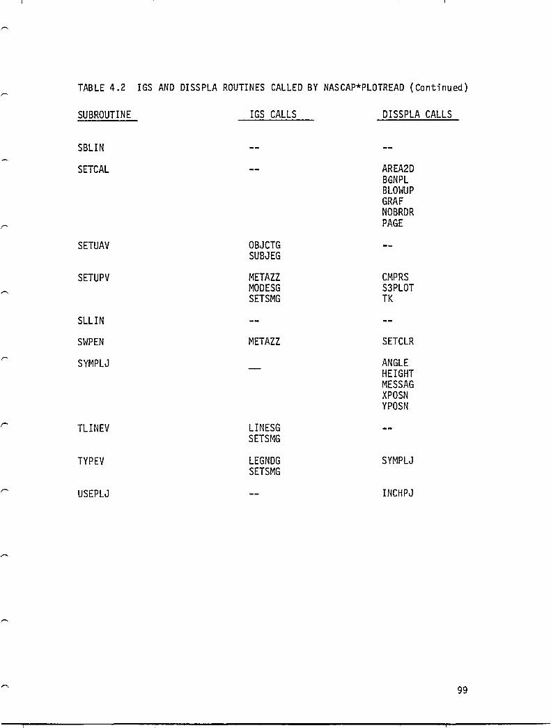
TABLE 4.2 IGS AND DISSPLA ROUTINES CALLED BY NASCAP*PLOTREAD (Continued)
SUBROUTINE IGS CALLS DISSPLA CALLS
SBLIN
SETCAL AREA2D BGNPL BLOWUP GRAF NOBRDR PAGE
SETUAV OBJCTG SUBJEG
SETUPV METAZZ CMPRS MODESG S3PLOT SETSMG TK
SLUN
SWPEN METAZZ SETCLR
SYMPLJ ANGLE HEIGHT MESSAG XPOSN YPOSN
r TUNEV UNESG SETSMG
TYPEV LEGNDG SYMPLJ SETSMG
USEPLJ INCHPJ
99

5. NASCAP*MATCHG
MATCHG is a code that models the current collection and charging response of a conducting sphere covered with a particular material. The purpose of the code is to give the user of NASCAP a general idea of how a complex object will charge by examining the response of a single surface material to a specified flux. The command structure of MATCHG has been reformulated into menu-type format. Rather than the code questioning the user for information repetitively, the user tells the code directly what is desired. As a result, he can change parameters and obtain revised answers with just one or two commands at any time.
MATCHG commands are entered as a string of keywords separated by spaces.
1.
2. 3.
The first keyword in a string is one of commands listed below. Input Commands ('LIST', 'CHANGE', 'PARAMETERS') Output Commands ('PLOT', 'TABLE', 'RESULT') Utility Commands ('HELP', 'EXIT')
Table 5.1 summarizes the command functions. Table 5.2 summarizes the command syntax.
100
-

1.
2.
3.
4.
5.
6.
7.
8.
Command
LIST
CHANGE
PARAMETERS
PLOT
TABLE
RESULT
HELP
EXIT
TABLE 5.1. MATCHG COMMANDS
Purpose
Display a specific set of parameters
Change a specific set of parameters
Summarize input parameters
Display a result in graphical form
Display a result in tabular form
Summarize a specific result
Display user information and guide
Exit MATCHG
~
INPUT
INPUT
INPUT
OUTPUT
OUTPUT
OUTPUT
UTILITY
UTILITY
101

...... a N
)
First Word Second Word
PARAmeters
LIST
LIST
LIST
LIST
LIST
LIST
CHANge
CHANge
CHANge
CHANge
CHANge
CHANge
J
MATErial
PROPerty
ENVIronment
ANGLe
EMISsion
VBACk VINIt VBEGin VEND
MATErial
PROPerty
ENVIronment
ANGLe
EMISsion
VBACk VI NIt VBEGin VEND
) )
TABLE 5.2. COMMAND FORMATS
Other Input
<#> to <#> or ALL
<new material>
<#> to <#> or ALL
<new envi> or «envi parameter><value»
<new angle> or «angle parameter><value»
ANGLe or NORMal
<potential>
) ) I)
Function
Summarizes parameters
Display input material
List material properties
Display input environment
Display angular distribution
List emission formulation
Backplate potential
IInitial sample potential I IV plot beginning and ending
potentials
Changes input material
Changes material properties
Changes environment
Changes angular distribution
Changes emission formulation
Same as LIST
J J ) J

...... o w
) ) ) 1
TABLE 5.2. COMMAND FORMATS (Continued)
First Word Second Word
RESUlt CHARge
RESUlt CURRent
TABLe
TABLe
TABLe
PLOT
HELP
EXIT
CHARge
IV
SECOndary BACKscatter ION ALL
(same as TABLe)
<Category (optional»
Other Input Function
FULL (optional) Summarize final potential
<potential> Currents at this potential
Summarize potential calculation
Current versus potential
Yields for these processes
Graph format
Assist user
Leave MATCHG
) )

5.1 PROGRAM STRUCTURE
Upon execution of MATCHG, the main program initializes the input parameters to a set of default values. These are listed in Table 5.3. The program is now ready to branch to seven different modules, including the HELP module, under the user's control at any time. Figure 5.1 shows the basic program structure of MATCHG. A table briefly describing the subroutines that handle user/code interfacing appears as Table 5.4. After entering EXIT, the user may obtain a hard copy of his run.
104
Property
Material
Angle
Environment
NE1, NIl
TEl, TIl
Emission
VBACK
VINIT
VBEGIN
VEND
TABLE 5.3.
Logical Unit Numbers;
Material Data File
Spectral Data File
Anisotropy Data File
INITIAL DEFAULT VALUES
Value
KAPT
Isotropic
Single
106 m-3
1. keY
Angle
o. keY
O. keV
O. keV
5. keY
8
9
10

)
...... a 01
) J )
INIT
)
.........................
)
MATCHG (MAIN)
MTALK '
I I I I I
----L
BACK TO MTALK
1
IVPLOT
,-' 6fI',,,.,,
,
CHARGE ,
TERPLE
Figure 5.1. Block diagram of MATCHG.
)
CHARGE
BSCAT PROSEC
-'
ELSEC BSCAT
PROSEC
)
VINIT VBEGIN
VEND BACKPL
)

Routine
BACKPL
CENVIR
CHANGE
CHANGL
CRETRN
EMISSO
FINISH
HELP
INIKAP
INlMAX
INIT
LANGLE
LENVIR
LIST
MATCHG
MATERL
MTALK
106
TABLE 5.4. USER/CODE INTERFACING ROUTINES
Purpose
Lists/changes backplate potential
Changes environment parameters
Controls I CHANGE I command
Changes angular distribution parameters
Holds up output until user is ready
Lists/changes emission formulation
Hard copies MATCHG run
Gives interactive help to user
Initializes input kappa values to code values
Initializes input Maxwellian values to code values
Initializes MATCHG/sets defaults
Lists angular distribution parameters
Lists environmental parameters
Controls 'LIST ' command
Main program
Lists/changes material
Interacts with user for commands
Called By
MTALK, PARAME
CHANGE, INIT
MTALK
CHANGE
HELP
PARAME, LIST, CHANGE
MATCHG
MTALK, CHANGE, LIST
CENVIR
CENVIR
MATCHG
LIST, CHANGL
LIST, CENVIR
MTALK
INIT, LIST, CHANGE
MATCHG

Routine
PARAME
PLOT
PROPER
RESULT
TABLE
VBEGIN
VEND
VINIT
TABLE 5.4 USER/CODE INTERFACING ROUTINES (Continued)
Purpose
Summarizes parameters
Controls 'PLOT' command
Lists/changes material properties
Controls 'RESULT' command
Controls 'TABLE' command
Lists/changes beginning plot potential
Lists/changes ending plot potential
Lists/changes initial sample voltage
Call ed By
MTALK
MTALK
LIST, CHANGE
MTALK
MTALK
MTALK, PARAME
MTALK, PARAME
MTALK, PARAME
107

5.2 MATCHG HELP
WELCCME TO ·~ATCHG't A MAT~RIAL CHARGING PROGR~~. TYPE 'HELP' AT ANY TI~E FOR ASSISTANCE. MATERIAL IS KAPT ENVIRON~ENT ~ow SI~GLE ~~XAELLIAN
HELP
wELCOME TO HELP. CHOOSE JN~ OF THE FOLLOWING CATAGOPIES BY ENTERING O~E OF THE 5 KEYWORDS SHOWN 1) SU~MARY
(AN OVERVIE~ OF ~ATCH5)
Z) INPUT (WHAT GOES IN?: ENVIRO~~E~T, PROPERTIES ANGULAR DISTRIBUTION, A~O MISC. PA~A~ETERS)
3) OUTPUT (WHAT CO~ES OUT?: CHA~GINGt CUQPENTS, IV (CURRENTS VS. VOLTAGE), AND YIELDS)
~) COM~ANDS
(HOW DO I GET WHAT I WANT?: CHANGE, LIST, PARA~ET~RSf R~SULT, TAalE, A~D PLOT)
5) RETURN (BACK TO PROGRA~J
? *** SUM~ARY ***
MATCHG ~ODELS THE RESPONSE OF A PARTICULAR ~ATERIAL
TO A SPECIfIED PLASMA ENVIqO~MENT. THE PARA~ETERS DESCRIBE 80TH THE ~ATERIAL A~O E~VIRONM~NT, A~D MAY BE SUPPLIED 8Y THE USER. All HAVE BEEN GIVEN DEFAULT VALUES. ON THE BASIS OF THIS INPUT, ~ATCHG wILL CALCULATE POTENTIALS AND CURRENTS AS RECUESTED ey THE USEQ
MATCHG CO~~ANDS A~E ENTERED ~S STPINGS OF KEY~OqoS, SEPARATED gy SPACES. THE FIRST KEYwORD IN A STRING CORRESPONDS TO ONE OF THE FOLLOwING CO~~ANDS
'LIST' - DISPLAY A SP~CIFIC SET OF PARA~ETEPS,
'CHANGE' - CHANGE A SPECIFIC SET OF PAR~METERS. 'PARA~~TERS' - DISPLAY A SU~~ARY OF INPUT PARAMETERS,
'PLOT' - DISPLAY A SP~CIFIC RESULT IN GRAPH FOR~.
'TABLE' - DISPLAY A qESULT I~ TABULAR FORM. 'P~SULT' - DISPLAY A °A~TICULAR ~ESUlT.
HIT RETURN <CR) TO CO~TINUE ALL KEY.OROS ARE SIGNIFICA~T TO 4 CHARACTERS (E.G. 'TABLE'='TA8L') INTEqNALLY. ADDING EXTRA CHARACTERS HAS NO EFFECT. TH~ FIRST THREE CO~~ANDS REFER TO USEq I~PUT. TYPE tI~PUT' FOR INFORMATION CO~CERNING THEIR USE.
108

THE LAST THREE REF~R TO OUTPUT. TYPE ·OUTPUT' FOR INFORMATION CONCER~ING THESE,
TO EXIT AT ANY TI~E, TYPE 'EXIT·, A HARD COpy OF YOUR ~OqK CAN BE REQUESTED, ?
*** INPUT «"'''' INPUT KEYWORDS FOLLOW 'LIST', AND 'CHANGE'
COMMANDS. THEY ARE:
1) ENVIRON'1ENT
SPECIFIES THE PLAS~A EN~RGY SPECTRUM TYPE. IT IS ANOTHER OF THE FOLLOWING .OQDS:
Al 'TANK' - TEST TA~K ENVIRON~ENT B) 'SINGLE' - ONE COMPONE~T MAXwELLIAN DISTqI9UTIO~ C) 'DOUBLE' - TWO COM?O~E~T MAXWELLIAN DIST~IBUTICN 0) '~ULTIPLE' - MULT. MAX~ELLIAN DISTRIBUTION (UP TO 5) E) '~APPA' - OISTqIBUTIC~ (OESCRETIZED ~AX~ELLIAN) F) 'OIRECT' - I~PUT Or TABULATED SPECTRAL DATA
FOR FURTHER I~FORMATICN ABOUT ~~ E~VIRON~ENT, E~TEP THE RELEVANT KEYWORD, OR HIT R~TURN TO CONTINUE. ?
2) ANGLE REFERS TO THE ANGULAR DIST~I~UTION OF THE INCOMING PLAS~A FLUX. IT IS FOLLOwED 3Y ONE OF FOUR KEYWORDS:
A' ISOTROPIC -B) ALIGNED - FIXED ANGLE OF I~CIDENC~ CJ ANISOTRCPIC - SUPERI~POS!D ISOTPOPIC AND OIQECTEO
FLUX. PA~AMETEqS AQE E~TERED I~TE~ACTIVELY D) FILE - ANISOTROPIC FLUX ~HEQE ENERGY DEPENDA~T
PARAMETERS ARE READ FROM A DATA FILE.
FOR FURTHER INFOQMATION ABOUT AN ANGL£ TYPE, ENTEP THE RELEVSNT KEYWORD, OR HIT RETURN TO CONTINUE ?
3) PROPERTY
REFERS To THE pqOPEDTIES ~F THE MATE~IAL CHOSEN. THE USER ~AY ENTER A NE~ ~ATERIAL BY TYPI~G:
'CHANGE ~ATE~rAL <~ATERIAL ~AME)' ANY NA~E, SIGNIFICANT TO FOUR CHARACT~RS. DEFINED ON DATA FILE 8, ~AY BE S~ECIFIED. PARTICULAR PQQPERTIES ARE REFER ED TO 8Y NU~3ER (1-14). TO REVIEw ~ATEPIAL pqOPERTIES, RETUR~ TO pOOGRA~ AND TYPE: 'LIST pqOPERTIES ALL'.
109
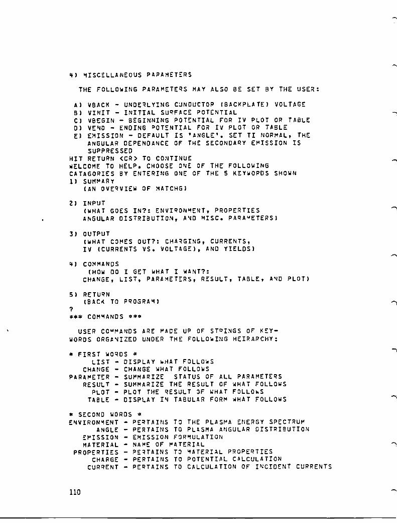
~) ~ISC~LLANEOUS PAPAMET~RS
THE FOLLO~ING PARA~ETE~S HAY ALSO BE SET BY THE USER:
A) VBACK - UNDE~LYING C~NDUCTOP (BACKPLATE} VOLTAGE S) VINIT - INITIAL SUqFACE POTENTIAL C) V8EGIN - BEGINNING POTENTIAL FOR IV PLOT OR TABLE 0) VE~O - ENDING ~OTENTIAL FO~ IV PLOT OR TABLE E) EMISSION - DEFAULT IS 'ANGLE'. SET TI NORMAL, THE
ANGULAR DEPENDANCE OF THE SECONDARY E~ISSION IS SUPPRESSED
HIT RETURN <CR) TO CONTINUE _ELCOME TO HELP. CHOOSE ONE OF THE FOLLOWING CATAGORIES BY ENTERING ONE OF THE 5 KEY~OPDS SHOWN 1) SUH~ARY
(AN OVEqVIEW OF MATCHG)
2) INPUT (WHAT GOES IN?: ENVIqON~ENT, PROPERTIES A~GULAR DISTRIBUTION, A~D MISC. PARA~ETERSJ
3) OUTPUT (WHAT C~~ES OUT?: CHA~GING, CURRENTS, IV (CURRENTS VS. VOLTAGE), AND YIELDS)
4} COMMANDS (HOW 00 I GET wHAT I WANT?:
CHANGE, LIST, PARAMETERS, RESULT, TABLE, AND PLOT)
5) RETUqN (BAC~ TO PQOGRA~)
?
*** COM~ANDS *** USER Cow~ANDS ARE ~ACE UP OF STQINGS OF KEY
WORDS ORGA~IZED UNDER THE FOLLO~ING HEIRARCHY:
* FIRST WORDS * LIST - DISPLAY wHAT FOLLOwS
CHANGE - CHANGE WHAT FOLLOWS PARA~ETER - SU~MARIZE STATUS OF ALL PARAMETEqS
RESULT - SUMMARIZE THE RESULT OF ~HAT FOLLOWS PLOT - PLOT THE qESULT JF WHAT FOLLOwS
TABLE - DISPLAY I~ TABULAR FOR~ WHAT FOLLOWS
* SECOND WORDS * E~VIRON~ENT - PEqTAIHS TO THE PLAS~A ENERGY SPECTRU~
ANGLE - PERTAINS TO PLASMA ANGULAR DISTRIBUTION E~ISSION - EMISSION FOR~ULATION MATERIAL - NA~E OF ~ATERIAL
PROPERTIES - PE~TAINS TO ~ATERIAl PROPEQTIES CHARGE - PERTAINS TO POTENTIAL CALCULATION
CURqENT - PERTAINS TO CALCULATION OF I~CIOENT CURRENTS
110

IV - PEqTAINS TJ CALCULATION OF CURR~NTS ~S A FUNCTION OF SURFACE POTENTIALS
HIT RETUR~ (Cq) TO CO~TI~U~
SECONDAqy \ BACKSCATTER' PERTAIN TO YIELDS FOR ION I THESE PROC~SSES ALL I
V9E6IN \ PEqTAINS TO TH~ ~A~G~ OF POTE~TIALS
VEND I FOR 'IV· CALCULATIONS
VSACK \ PERTAI~S TO INITIAL POTENTIAL IN A VINIT I CHARGE CALCULATION HIT RETURN <CR) TO CONTI~uE
* SUBSEOUE~T WORDS AND DATA * SOME CO~MANCS CAN 3E APPENDED ~ITH DATA STRINGS AND/OR ADDITIONAL WORDS ~HERE APPROPRIATE E.G.:
'CHANGE VBEGIN -2.' (CHANGE THE PARAMETER V9~GIN TO -2. KEV)
'LIST PROPERTIES 2 7' (LIST THE VALUES OF ~AT~RIAL PROPERTIES :-7)
'RESULT CHARGE FULL' (DISPLAY THE CHA~GING ~ESULT OF THE SAMPLE, AND
HAVE A 'FULL' SUMMARY OF CUqRENTS AT EACH TIMESTEP)
'CHANGE ANGLE FILE IC' (CHANGE A~GULA~ JISTRI3UTION TO ANISOTROPIC PARA~ETERS
FROM FILE l~)
'CHANGE ENVIRON~ENT TEl 2' (CHANGE E~VIqONMENTAL EL~CTqON TE~EqATURE 1 TO 2 KEV) HIT RETURN <CP) TO CONTI~U~
_ELCOME TO HELP. C~OOSE ONE OF THE FOLLOWING CATAGOPIES BY ENTERING O~E OF THE 5 KEYwORDS SHO~N 1) SUMMAPY
(AN OVEqVIEW OF ~ATCHG)
2) INPUT (WHAT GOES IN?: ENVIRON~E~T, PROPERTIES ANGULAP OISTqIBUTION, A~D ~ISC. PARA~ETERS)
3) OUTPUT (WHAT CO~ES OUT?: CHAqGING, CJRRENTS, IV (CURRENTS VS. VOLTAGE), AND YIELOS)
"J CmH"aNDS (HOW DO I GET ~HAT I ~ANT?:
CHANGE, LIST, PARAMET~qS, RESULT, TABLE, ANO PLOT}
5J RETUR~
•
111
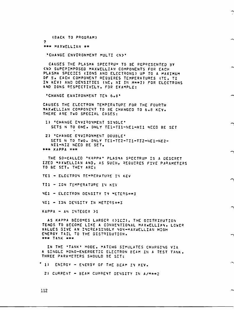
(SACK TO PROGRAM) ? *** MAXWELLIAN **
'CHANGE ENVlqONHENT ~ULTI {N)'
CAUSES THE PLASMA SPECTqU~ TO BE REPqESENTED 9Y CN) SUPEPIMPOSED MAXWELLIAN COMPONENTS FOR EACH PLASMA SPECIES (IONS AND ELECTRONS) UP TO A MAXIMUM OF 5. EACH COMPONENT RECUIRES TEMPERATURES (TE, Tl IN KEV) AND DENSITIES (NE, NI IN H**3) FOR ELECTRONS AND IONS qESPECTIV~LY. F~R EXA~PLE:
'CHANGE ENVIRONMENT TE4 6.8'
CAUSES THE ELECTRON TEMP~RATUPE FOR THE FOURTH MAX~ELLIAN COMPONE~T TO 3E CHANGED TO 6.8 KEV. THERE AqE TwO SPECIAL CASES:
1) 'CHANGE E~VlqO~~ENT SI~GLE'
SETS N TO ONE. ONLY TE1-TI1-NE1-NIl ~EED BE SET
2J 'CHANGE E~VIRONMENT DOUBLE' SETS N TO TWO. ONLY T~1-T~2-TII-TI2-NE1-NE2-NI1-NI2 NEED BE SET.
*** KAPPA 'lr'lr*
THE SO-CALLED 'KAPPA' PLAS~A SPECTRU~ IS A DESCRET IZEO ~~xWELLIAN AND, AS SUCH, ~ECU!RES FIVE PAqAMETERS TO BE SET. THEY ARE:
TEl - ELECTRO~ TE~oERATU~E I~ KEV
TIl - ION TEHPEqATURE I~ KEV
KAPPA - A~ I~TEGER >1
AS KAPPA BECO~ES LARGE~ ()lC:), THE DISTRIBUTIO~
TENDS TO BECOME LIKE A C~NVE~TIONAL HAXwELLIA~. LOWER VALUES GIVE AN I~CQE~SINGLY ~O~-MAxwELLIAN HIGH ENERGY TAIL TO THE DISTQIBUTIGN. *** T4Nr( ***
IN THE -TANKe MODE, ~ATCHG SI~ULATES CHARG!~G VIA A SINGLE ~C~O-ENERGETrC ELECTRON EEA~ IN A TEST TANK. THREE PARA~ETERS SHOULD 8E SET:
• 1) EN~RGY - E~ERSY OF THE BEA~ I~ KEV.
2) CURRE~T - BEAM CURRE~T DE~SITY IN A/M~~2
112 ....
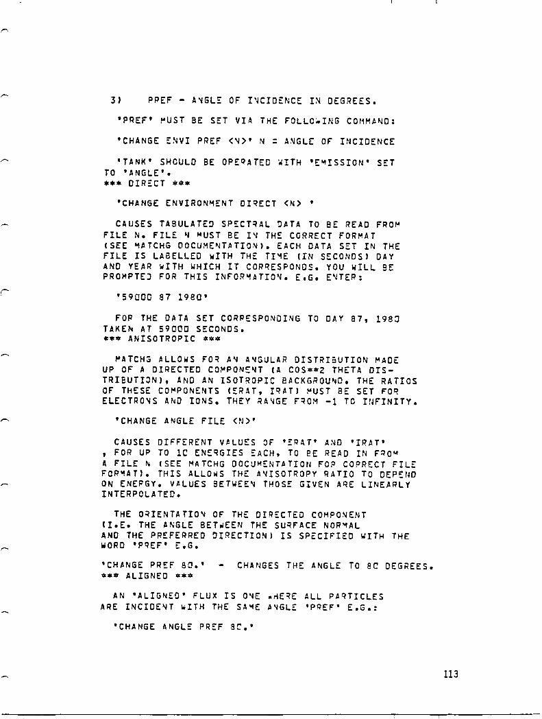
3) PPEF - A~GL~ OF I~CIDENCE I~ DEGREES.
'PREF' ~UST BE SET VIA THE FOLLC~ING COHM~~D:
'CHANGE ENVI PREF (~)~ N = ANGLE OF INCIDENCE
'TANK' SHCULD 8E OPEqATED ~ITH 'E~ISSION' SET TO 'ANGLE~ • • ** DIR~CT ***
'CHANGE ENVIRON~ENT OIqECT {N> •
CAUSES TABULATED SP~CT~AL ~~TA TO 8E READ FRO~
FILE N. FILE ~ ~UST BE I~ THE CORRECT FORMAT (SEE ~ATCHG OOCUME~TATION). EACH DATA SET IN THE FILE IS LABELLED wITH THE n"lE CIN SECONDS J DAY AND YEAR wITH WHICH IT COPqESPONDS. YOU WILL 9E PROMPTEJ FOR THIS INFOR~ATIO~. E.G. E~TER:
'59QOO 87 1980'
FOP THE DATA SET CORRESPONDING TO DAY 87, 198~ TAKE~ AT 59000 SECONDS. *** ANISOTROPIC ***
~ATCH3 ALLOwS FO~ A~ A~GULAR DISTRIBUTION ~ADE UP OF A DIRECTED CO~PONE~T (A COS**2 THETA OISTRIEUTIJNJ, AND AN ISOTROPIC eACKGROU~D. THE RATIOS OF THESE CO~PONENTS (ERAT, rqATJ ~UST BE SET FOq ELECTRO~S A~D IONS. THEY RA~GE FQCM -1 TC INFINITY.
'CHANGE ANGLE FILE (N)'
CAUSES DIFFERENT VALUES OF 'EPAT' AND 'IRAT' , FOR UP TO lC ENEqGIES EACH, TO eE READ IN F~O~
A FILE ~ (SEE MATCHG DOCUMENT~TION FOP COPRECT FILE FOR~AT). THIS ALLO~S THE A~ISOTROPY RATIO TO DEPEND ON ENEPGY. VALUES 9ETWEE~ THOSE GIVEN AqE LINEARLY INTERPOLATED.
THE O~IENTATIO~ OF THE DIRECTED COHPONENT (I.E. THE ANGLE BET.EEN THE SUqFACE NOR~AL AND THE PREFERRED DIRECTION) IS SPECIFIED WITH THE WORD 'pqEF' E.G.
'CHANGE PREF ao.' *** ALIGNED ***
CHANGES THE ANGLE TO 8e DEGREES.
AN 'ALIGNED' FLUX IS O~E .~E~E ALL P~qTICLES
ARE INCIDE~T .ITH THE SA~E A~GL£ 'PREF' E.G.:
'CHANGE ANGLE PREF ac.'
113
CHANGES THE ANGLE OF I~CID~NT TO 8~ DEGREES. *** ISOTROPIC ***
WHEN THE ANGL~ TYPE IS ISOTROPIC, THE FLUX IS INCIDENT ~ITH ALL ~NGLES BEI~G ECUALLY PRO~AeLE. NO ADDITIONAL PARAMETEPS ARE IMPLIED.
EXIT
(EXITl
114

5.3 INPUT
The MATCHG input parameters describe the physical properties of the material and the surrounding plasma environment. There are five basic types of input which may be specified.
1. 'ENVIRONMENT ' specifi es the plasma energy spectrum
2. I ANGLE I angular distribution of incoming flux
3. I MATERIAL I surface material at hand (see Table 5.5).
4. I PROPERTIES I properties of the material (1-14)
5. 'MISCELLANEOUS ' potential parameters for the calculations: 'VBEGIN', 'VEND', 'VBACK', and 'VINIT '
One of these words must follow a 'LIST ' or I CHANGE I command word. (See HELP in Section 5.1.1 for more details.)
115
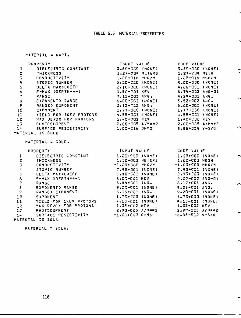
TABLE 5.5 MATERIAL PROPERTIES
tcATERIAL = KAPT.
PROPEQTY I~PUT VALUE CODE VALUE 1 DIEL::CTRIC CONSTANT 3.5G+GC~ (NONE) 3.50+000 (~O~EJ
---2 THICKNESS 1.Z7-~:Jq METEQS 1.27-(lC4 MESH ! CO'lDUCTIVITY l.Ce-C16 t'HO/~ 1.00-016 MHOIM 4 ATOMIC NUMBER 5.0C+COC (NONE) S.OO+O~O ("40NEJ 5 DELTA MAX>COEFF 2.1C+CCO (N 0 NE ) 4.Q6+0:l1 ('lO"'E) E: E-MAX >DEPTH**-l 1.5C-C:ll KEV 8.74-002 A"'G-Ol 7 PANGE 7.15+001 ANG. 4.29+001 A'IG. 8 EXPONENT) Q ArJGE 6.CQ-COl (NONE) 5.52+002 ANG.
']
9 RANGE> EXPONE~T 3.12+r:2 ANG. 6.00-00! (~ONE)
11: EXPONENT 1.77+0CO (NONE) 1.77+COO ('lONE) 11 YIELD FOR lKEV P~OTO'lS ~.55-0~1 (~ONE) 4.55-C:::1 ''lONE) 12 ~AX DE/OX FOR P~OTONS 1.4:::+('02 KEV 1.40+C02 KEV 13 PHOTCCURRE'IT 2.CO-CG5 A/'1**2 2.CO-O:15 A/M**2 14 SURFACE qESISTIVITY 1.CC+C16 OHfo1S 8.85+0::14 V-S/Q
..,ATERIAL IS GOLD
MATERIAL = GOLD.
PROPERTY INPUT VALUE CODE VALUE 1 OIEL!:CTRIC CO'lSTANT 1.:JC+t;cC (NONE) 1.~O+Cac ('lO'lE) 2 THICKNESS 1.:C-OC3 METERS 1.0e-003 MESH 3 CONDUCTIVITY -l.OO+Ct:C f"HO/t' -l.OC+fJCO MHO/'" 4 ATOI'4IC NU'19ER 7.9Q+OCl (NONE) 7.9c+o::a P~O'lE)
5 DEL TA "'AX>COEFF a.80-C';1 (NONE) 2.93+:C3 ('40~E)
6 E--UX >DEPTH**-l s.aC-CGl KEV 2.02-0Q2 A~G-Ol 7 R~NGE 8.88+CCl ANG. 8.17+COl ANG. 8 EXPO~ENT> UNGE 9.'~-CC1 , NONE) 9.2S+CJl A'JG. 9 ~ANGE> EXPONENT S.35+CQl ANG. 9.20-COl (~O~E)
Ie EXPONEt-lT 1.73+C:JC (NONE) 1.73+000 (~ONE)
11 YI~L:l FOR 1l(EV C)~OTO'4S ~.13-CCl (NONE) u.l!-CJl {'lONE} 12 "4~X DE/OX FOR oqOT~~S 1.35+CC2 KEV 1.35+C02 KEV 13 PHOTOCURRENT 2.90-CGS A/M**2 2.9r,-JCS A/~**2 14 SUQFACE RESISTIVITY -l.ac+ccn OH~S -8.35-012 V-SIC
MATERIAL IS SOLA
~ATERIAL = SOLA.
116

PR::>PE~TY 1 DIEL~CTRIC CONSTANT 2 THICKNESS 3 CONDUCTIVITY 4 ATO~IC NUM3ER 5 DELTA MAX)COEFF 6 E-MAX )OEPTH~~-l
7 RA"4GE 8 EXPONENT) qANGE 9 RANGE> EXPONENT
10 EXPONENT 11 YI~LO FOR lKEV ?~OTO~S 12 MAX DE/OX rOR P~OTONS
13 PHOTOCURRENT 14 SURfACE RESISTIVITY
'1ATERIAL IS SCRE
foIATERIAL = SCRE.
PROPERTY 1 DIELECTRIC CONSTANT 2 THICKNESS 3 CO~DUCTIVITY 4 ATO~IC NU~9ER
5 DELTA MAX>COEFF 6 E-MAX >DEPTH~~-1 7 PANGE 8 EXPONENT> RANGE 9 RANGE) EXPONE~T
IE! EXPONENT 11 YIELD FOR 1KEV P~OTO~S 12 ~AX DE/OX FO~ PQOTONS 13 PHOTOCURRE~T
14 SURFACE RESISTIVITY '4ATEPIAL IS ASH
I'IAT::RIAL = ASTR.
PROPERTY 1 DIELECTRIC CO~STA~T 2 THICKNESS 3 CO~DUCTIVITY 4 ATOMIC NUMBER 5 DELTA MAX)CCEFF 6 E-~AX )OEPTH~~-1
7 ~A"lGE 8 EXPONE~T> qANGE 9 RANGE) EXPONENT
10 EXOONENT 11 YIELD FOR lKEV pqaTONS 12 ~AX DE/DX FOR pqOTONS 13 PHaT~CURqE~T
14 SU~FACE RESISTIVITY ""ATERIAL IS TEFL
I~PUT VALUE 3.80+COC (NONE) 1.79-CG4 METERS 1.:l0-C17 P-'HO/M 1.:l0+C01 (NONE) 2.05+000 (NONE) 4.le-COt KEV 7.75+001 ANG. 4.50-C!Cll (NONE) 1.56+CC2 ANG. 1.73+CCO OIONE) 2.44-C~:l (NONE) 2.30+C02 KEV 2.CO-Ca5 A/i'1~~Z 1.01J+C19 OHMS
INPUT VALUE 1.CC+0:lC (NONE) 1.00-003 METERS
-l.GC+CCO MHOIM 1.GC+C::O (NONE) .~O (NONE)
1.0C+00C KEV 1.:0+0:1 ANG. 1.5C+OCO (NONE)
.CO ANG. 1.CQ+('CC (NONE)
.CO (NONE) 1.CO+('OO KEV
.Co A/"l~~2
-1.i:O+C~O OHMS
INPUT VALUE 3.80+0::0 (~ONE)
2.75-!:'C" METERS 2.75-012 "'HOlM 1.uc+rOl (NONE) 2.'+C+CCO (~ONE)
4.CC-aOl KEV 6.75+001 ANG. 8 _lC-CC 1 (NONE) 1.06+C~2 ANG. 1.86+(':0 (NONE) 4.55-r:C1 (NONE) 1.40+CC2 KEV 2.DO-0:J5 A/"l~~2
1.00+011 OH"lS
CODE VALUE 3.8C+000 CNO~E)
1.79-00~ M:;SH 1.QO-017 MHOIM 1.00+001 (~O'4E)
1.31+001 (~ONE)
3.17-0J2 A'lG-01 3.49+001 A'lG. 2.70+0:J2 A'4G. 4.50-0in U., 0.., E ) 1.73+0iJO (NO"'EJ ~.44-0Cll ('lONE) 2.30+002 KEV 2.GO-OOS A/M.~2 8.85+Q07 V-SIC
CODE VALUE 1.00+000 ('lONE) 1.00-0C3 MESH
-I.OO+COC' MHO/M 1.CO+COO ('10'lE)
.0£1 ('10"'E) 1.38-001 A'lG-Ol 1.50+001 A"'G.
.... ,. • -.iU
1.50+000 I.CO+Cao .aa
1.00+000
A'IG • ('lONE) (~O'l E> ('lONE) KEV
.GO AIM~~2
-8.8S-CH2 V-SIC
CODE VALUE 3.8C+OCC ('lONE) 2.75-004 M~SH 2.75-012 M"fO/M 1.00+001 ('lO'lE) 1.46+001 ('lONE) 3.a1-0iJZ A"'G-01 5.47+0::11 A'lG. 1.97+002 A ~IG. 8.10-001 (..,ONE) 1.86+0iJO ('lO~E)
4.55-001 (NONE) 1.40+C02 KEV 2.00-005 A/M*~2 8.85-C:n V -S/Q
117
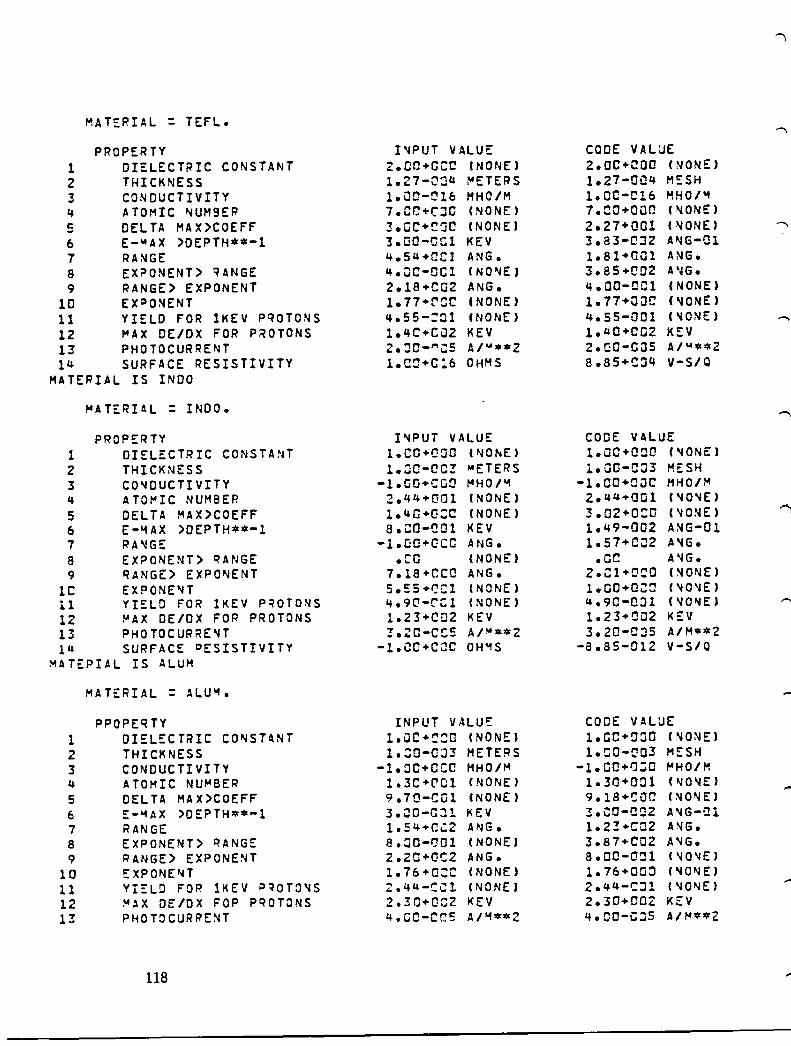
MAT::RIAL = TEFL.
PROPERTY I'4PUT VALUE CODE VAL~E 1 DIELECTRIC CONSTANT 2.00+0:0 (NONE) 2.DC+COO (NONE) 2 THICKNESS 1.27-C':J4 r-tETERS 1.27-Q04 M::SH 3 CONDUCTIVITY 1.iJO-~16 MHOIM 1.CO-C16 MHOI'" 4 ~TOMIC ".IUH9EP 7.CC+C':JO (NONE) 7.CO+oon (~ONE)
5 DEL TA MAX)COEFF 3.GC+C~C (NONE) 2.27+001 (~ONE) ---6 E-"'AX >DEPTH**-l 3.aO-OCl KEV 3.83-0J2 A~G-01 7 RANGE 4.54+0Cl ANG. 1.81+Q01 ANG. 8 EX?ONENT) ~ANGE 4.aC-OCl (NO'lE) 3.85+002 A '~G. 9 RANGE) EXPONENT 2.18+(:02 ANG. 4. aO-Oin (NONE)
10 EX:)O~ENT 1.77+r'CC (NONE) 1.77+000 ('lONE) 11 YIELD FOR lKEV pqOTONS 4.55-:01 (NONE) 4.55-Q01 (~ONE)
12 "'AX DE/OX FOR PROTONS 1.4C+CJ2 KEV 1."0+002 KEV 13 PHOTOCURRENT 2.::!0-"'~5 A/"'**2 2.QC-C05 A/"'**2 14 SURFACE RESISTIVITY 1.C~+C:6 OHMS 8.85+C~4 V-S/Q MATERI~L IS INDO
"'ATERI~L = INDO.
PROPERTY I~PUT VALUE CODE VALUE 1 DIELECTRIC CONSTANT 1.CO+GOO ("lOhE) 1.00+000 ('lONE) 2 THICKNESS 1.OO-CO! "'ETERS 1.aO-C:J3 MESH 3 CO~DUCTIVITY -l.GQ+CGO ,..HOI'" -1.00+000 MHOI'" 4 ATO,..IC NUMBER 2.44+001 (NONE) 2.44+001 ('40'40 5 DELTA MAX>COEFF 1.40+Q:C (NONE) 3.02+0::0 ('JONE) 6 E-"'AX )OEPTH**-1 a.CO-COl KEV 1.49-002 ANG-Ol 7 RA'-JGE -l.C:O+QCO ANG. 1.57+002 A~G. 8 EXPONENT) ~ANGE • CO (NONE) '"'" A'IG • ........ 9 qANGE) EXPO"lENT 7 al8 +CCQ ANG. 2.~1+oca (NOlliE)
11: EXPONE"JT 5.~5+~Cl (NONE) 1.GO+Oi::O ('40'4E) 11 YI::LD FOR lKEV P~OTO~S 4.9(1-(':1 (NONE) ~.9C-CJ1 ('10~E)
12 ~AX DE/OX FOR PROTONS 1.23+C02 KEV 1.23+a02 KEV 13 PHOTOCURRE'4T !.2C-CCS A/~"'*2 3.20-0:)5 A/"'**2 1" SURFACE °ESISTIVITY -1.CO+C~C OH'1S -8.85-012 V-SIC ~ATEPIAL IS ALUM
MATERIAL = ALU"'.
PPOPEqTY INPUT VALU:: CODE VALUE 1 DI!::LECTiHC CO~STANT l.ac+c:o (NONE) 1.0C+~:JO (~O~E)
2 THICKNESS 1.:0-0;)3 METERS 1.:;0-003 MESH 3 CONDUCTIVITY -l.:JO+OCC MHO/M -1.CiO+Ij;O "'HOlM 4 ATOMIC NU"'BER 1.31:+('(;1 (NONE) 1.31J+0~1 (1II0'lE) 5 DEL TA MAX)COEFF 9.7Q-CCil (NONE) 9.18+~iJC (NO'lE) 6 ::-"UX )DEPTHlOt*-1 3.~0-CJl KEV 3.CO-O!!Z A'IG-':n 7 RANGE 1.S~+C~2 AIIIG. 1.2!+C02 A~G. 8 EXPONENT> ~ANGE 8 • ::lO -IJ 0 1 (NONE) 3.87+002 A'4G. 9 RANGE> EXPONENT 2.20+0C2 ANG. 8.00-0~1 ('JO'lE)
10 EXPONE~T 1.76+0:C (NONE) 1.76+00::3 ('IO~E)
11 YI::LD FOR IKEV o~OTO'JS Z.4~-~C1. (1II0NE) Z.44-CJl ('IO'lEJ 12 ~AX DE lOX F'OP PQOTONS 2.30+QC2 KEV 2.30+002 KEV 13 PHOTOCURRE~T 4.CC-CCS A/"'*0012 4.00-C:5 A/M**2
118
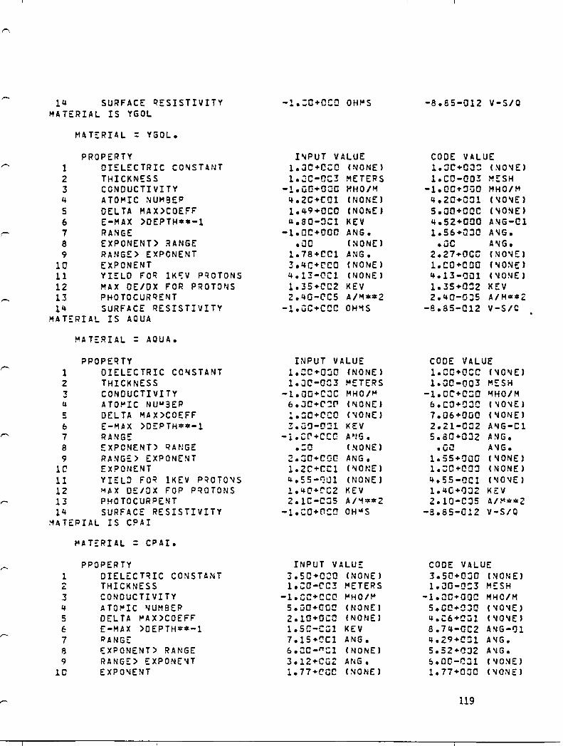
14 SURFACE q::SISTIVITY -l.:o+cca OH"'S -8.85-012 V-SIC MATERIAL IS YGOL
MAT:;RIAL = YGOL.
PROPERTY I'lPUT VALUE CODE VALUE 1 OIEU:CTRIC CONSTANT 1.JC+Ci:C (NONE) 1.::1C+OO: n~O'lE)
2 THICKNESS 1. ~C-!H:3 METERS l.CO-OO! M~SH 3 CONDUCTIVITY -l.Go+oao MHO/M -l.QC+~QO MHO/'" 4 ATOMIC ~UM8EP 14.2C+C01 (NONE) 4.20+001 ('lO'lE) 5 DEL TA MAX)COEFF 1.49 +CCC (NONE) 5.CO+CCC ('lONE) 6 E-MAX >OEPTH**-l u.80-:JC1 KEV 4.52+000 ANG-C1
i' 7 RANGE -1.0C+000 ANG. 1.56+0JO A"IG. 8 EXPONENT> RANGE .00 (NONE) • oc A~G • 9 RANGE> EXPONENT 1.78+CC1 ANG. 2.27+0CC (NO'lE)
10 EXPONENT 3.4C+CCO (NONE) 1.CO+COO ('lONE) 11 YIELD FO~ 1Kc:.:V PQOTONS 4.13-0C1 (NONE) 4.13-001 ('lONE) 12 MAX OEIOX FOR PROTONS 1.35+CC2 KEv 1.3S+0~2 KEV 13 P!-+OTOCURQENT 2.4Q-CCS A/M**2 2.40-0:)5 A/M**2 14 SURFACE RESISTIVITY -l.GC+CCC OH~S -8.85-012 V-SIC
MAT:::RIAL IS AOUA
,..AT:::RIAL = ACUA.
PPOPEqTV INPUT VALUE CODE VALUE 1 DIELECTRIC CO"4STANT 1.CC+O:lQ (NONE) 1.CC+OCC (~O'lE)
2 THICI<NESS 1.JC-OC3 "'ETERS 1.aO-OQ3 MESH 3 CONDUCTIVITY -l.QQ+COC MHO/"- -1.0('+0:;0 MHO/M u ATO"'IC Nu w3EP b.JO+C~('I (r-tONE) b.CO+CJO ('lO"lE) c: DEL TA MAX>COEFF :'.:::O+CCO ('lONE) 1.06+000 ('lONE) ... 6 E-M.AX >DEPTH**-l ~. oa-o:n KEV 2.21-0:2 A~G-C1 1 RANGE -l.~r+ccC! A ~tG • 5.80+0J2 A~G.
8 EXPONENT) qANGE .:0 (NONE) • GO A'IG • 9 RANGE> EXPONENT 2.:J0+CO~ ANG. 1.55+000 ('lONE)
lC EXPONENT 1.2C+CC1 P~ONE ) 1.:JC+OO:J (NONE) 11 YIELD FO~ lKEV P'?OTO'lS 4.SS-l'hJl (NONE) 4.SS-0Cl (~O'lE)
12 "'.AX DEIOX FOP PQOTONS 1.4C+!'C2 KEV 1.40+1):)2 KEV 13 P!-+OTOCURPENT 2.1C-C:JS A/"l**2 2.10-CJ5 A/~**2
14 SURFACE RESISTIVITY -l.co+('!ca OHIoIIS -8.85-(H2 V-S/O !'1ATEPIAL IS CPAI
M.AT~RIAL = CPAI.
PROPER TV INPUT VALUE CODE VALUE 1 DIELECTtHC CONSTANT 3.50+0:0 (NONE) 3.SQ+Q:lO (~ONE)
"" THICKNESS 1.:0-CC! "'ETERS 1.;:JO-O:3 M::SH L
3 CONDUCTIVITY -1.GC+CCC /oIHO/r-' -1.00+000 MHC/M 4 AT01'4IC ~UMBEP s.ao+oac (NONE) 5.0Q+OJO ('lO'lE) 5 DEL TA r-'AX>COEFF 2.10+0CC (NONE) 4.C6+0ul ("IO'lE) l: E-MAX >DEPTH**-1 1.5C-C~1 KEV 8.14-0C2 ANG-lJl 7 PANGE 7.15+!;Cl ANG. 4.29+C!J1 A"4G. 8 EXPONENT) RANGE b.nO-"G1 (NONE) 5.52+0:12 A'IG. 9 RANGE> EXPONE"H 3.12+CiJ2 ANG. b.oc-c:n ("40~E)
10 EXPO~ENT 1.77+00C (~ONE) 1.77+000 ('JaNE)
119

11 VI::LD FOR lKEV P~OTO~S 4.5S-0Gl (NONE) ~.5S-ma (~ONE)
12 MAX DE lOX FOR pqOT:lNS 1.40+002 KEV 1.40+0J2 K::V 13 PHOTOCURqE"fT Z.::O-O~5 A/M"'*2 2.00-0::5 A/M**2 14 SURFACE RESISTIVITY -1.ao+~ac OHMS -8.85-012 V-SIC
MATERIAL IS VELO
~AT::Q!AL = VELD. -.,
PPOPERTY INPUT VALUE COOE VALUE 1 DIELECTRIC CONSTANT 3.5C+C::C (NONE) 3.50+000 (~O~E)
2 THICK~ESS 1.~0-OC3 ~ETERS 1.00-003 M::SH 3 CO~[iUCTIVITY -1.:0+COO MHO/M -l.GO+C;jO MHO/M 4 ATO~IC NUM3EP 5.!:C+CCO (NONE) 5.CO+CJO (~O~E)
5 DEL TA MAX>COEFF 2.10+000 (NONE) 4.C6+(101 (NO~E) ...... 6 E-~AX )OEPTH**-l l.se-OCI KEV 8.74-002 A~G-Cl 7 RANGE 7.15+~Ol ANG. 4.Z9+0ill ANG. 8 EXPCNE"JT> RANGE 6.~0-OCI (NONE) 5.52+:)02 A~G.
9 qANGE) EXPONENT 3.12+Q!J2 ANG. b.CO-OCI (~O'lE)
10 EXPONENT l.77+~CO (NONE) 1.77+000 ('lONE) 11 YIELD FO~ lKEV PQOTO'lS 4.55-CC1 (NONE) 4.55-001 ('IO'lE) 12 MAX DE/OX FOQ PROTONS l."Q+caz I<EV 1.4a+0~z KEV 13 PHOTOCURRENT 2.CC-!:!05 A/~**2 2.00-005 A/M**2 14 SURFACE RESISTIVITY -l.co+oac OHf'lS -8.8S-01Z V-SIC
MATERIAL IS ML12
MATERIAL = !"L12.
PPOPERTY INPUT VALUE CODE VALUE 1 DIELECTRIC CONSTANT l.co+can (NONE) 1.00+u:::0 ('40~E)
2 THICKNESS 1.:C-(HJ3 METERS 1.aC-C~3 M::SH 3 CO~DUCTIVITY -l.:C+CCC ~HO/p.t -1.JO+IJ~O MI.fO/M 4 ATO~IC NUM3ER 6.CQ+OCC (NONE) 6.CO+OCO ('10~E)
5 DEL TA MAX)COEFF 1.OC+CCO (NONE) 7.06+00:) ('IO~E)
6 E-"'~X >DEPTH**-l 3.:C-OCI KEV 2. 21-C:::l2 A'IG-01 7 PANGE -l.L::J+O:JO ANG. 5.80+0::3Z ~'1G.
8 EXPONE~T> ~ANGE -n ... - (~ONE) .el: A'IG. 9 RANGE> EXPONE'JT Z.::+!JCO A 'lG • 1.S5+0J~ ('10'lE)
10 EXPONENT 1.20+01:1 (NONE) 1.CO+COO ('10'lE) 11 YI::LD FOR 1KEV P~OTO'lS 4.55-CCl (~ONE) 4.55-0:)1 (NO~E)
lZ MAX DE/OX FOR P~OTONS 1.40+C:2 KEV 1.4Q+OCZ K EV 13 PHOTOCURRENT 2.1~-C:5 A/~"'*2 Z.lC-C::lS An'·*2 14 SURFACE RESISTIVITY -l.JIJ+cao OHMS -8.85-012 V-SIC
MATERIAL IS MAGN
~ATERIAL = MAGN.
PRQPEPTV INPUT VALUE CODE VALUE 1 DIELEC rq IC CC~STANT 1.::;O+O~C (NONE) 1.GC+OJC ('10'lE) - THIC!(NESS 1.JO-C:3 ~ETERS 1.0C-0:;3 "'::SH "" 3 CONDUCTIVITy -l.i:O+OCC MHO/~ -1.00+0:]0 MHO/'1 4 ATOMIC NU'19ER 1.2C+t:C1 (NONE) 1.2[j+IJJl (NO'lE) 5 OEL TA MAX>COEFF 9.2C-C~1 (NONE) 7.C2+Q!JO ('IO~E)
6 E-!'U X >DEPTH**-1 2.s~-ca1 I<EV 2.79-002 A'IG-Ol 7 RANGE -l.Jo+r:: ANG. &.96+00Z ANG.
120

8 EXPONE~T) ~ANGE
9 RANGE> EXPO~ENT 10 EXPONENT 11 YIELD FOR 1KEV ?~OTO~S 12 ~AX DE/OX FOR pqOTONS 13 PHOTOCURQENT 14 SURFACE RESISTIVITY
'1ATERHL IS NPAI
~ATERIAL = NPAI.
PROPERTY 1 DIELECTRIC CONSTANT 2 THICKNESS 3 CO~DUCTIVITY q ATOMIC NU~BER 5 DELTA MAX>COEFF 6 E-wAX )DEPTH**-1 7 RA'IGE 8 EXPONENT) ~ANGE
9 RANGE) EXPONENT 10 EXPONENT 11 YIEL~ FOR lKEV PQOTONS 12 ~AX DEIOX FOR PQOTONS 13 PHOTOCUqRENT 14 SURFACE RESISTIVITY
MATERIAL IS SILV
"'AT~RHL = SILV.
PROPEqTY 1 DIELECTRIC CC~STANT 2 THICKNESS ! CONDUCTIVITY 4 ATO~IC NUMBER 5 DELTA MAX)COEFF 6 E-~AX )DEPTH**-l 7 RA~GE
8 EXPONENT) qANGE 9 RANGE) EXPONE'IT
lC EXPONENT 11 YIELD FOq lKEV P~OTONS 12 ~AX DEIOX FOR pqOTONS 13 PHOTOCURqE~T
14 SURFACE qESISTIVITY MATERHL IS IlOGO
I'IATERIAL = POGO.
PROPERTY 1 DIELECTRIC CONSTANT 2 THICKNESS 3 CO~DUCTIVITY
4 ATOMIC NUM8ER
.ve P~ONEJ
1.74+c:r ANG. 2.43+0C1 (NONE) 2.44-C!Jl (NONE) 2.30+!J02 KEV 4.CO-CC5 A/M.*,
-l.Ol'1+CC(, OH~S
INPUT VALUE 3.so+cac (NONE) 5.0~-OCS "'ETERS 5.9C-Cl4 ,..HO/'" 5.:C+00IJ (NONE) ~.lO+COC (NONE) 1.se-COt KEV
-l.:C+CCO ANG. .:0 (NO~E)
1.0s+ca~ A~G.
9.Ba+cc~ (NONE) !.t.ss-eel (NONE) 1.4~+CC2 KEV 2.~O-OCS 4/11.*2 1.00+013 OHI1S
INPUT VALUe: 1.OO+C:j: (NONE) !.:~-~a~ f"ETERS
-1.:0+CGC MHOI'" 4.70+CCl (NONE) 1.CO+COC (NONE) 8 • 0 a -c C:l IC E V S.45+cn ANG. 8.20-001 'NONE} 7.94+r:n ANG. 1.74+GGC (NONE) 4.90-001 (NONE) 1.23+002 KEV Z.90-C~5 4/"1**2
-1.£:0+000 OH'1S
I"4PUT VALUE 1.OO+!:lCO (NONE) 1. ::lG-OJ3 METERS
-l.Jo+oao "'HOI'" 7.:n +rJOl (NONE)
.00 A'IG. 1.75+000 (~O'lE)
1.OC+CJC (~ONEJ
2. '+"-001 ("O~lE) 2.30+002 K;:V 4.00-005 A/I1**2
-8.85-012 V-SIC
CODE VALUE 3.5C+OOO (~O~E)
s.oo-cas ~~SH 5.90-014 MHO/M s.OC+O:)O (NO'lE) 3.05+001 P40~E)
3.41-0J2 ANG-C1 1.05+003 A'IG. .co A'IG.
1.51+00(1 ('10'lE) 1.00+000 ("O~E) 4.5S-0:Jl ("O~E)
1.40+002 KEV 2.ao-oes A/~**2 8.85+(;01 V-SIC
CODE VALUE 1.C(!+Q:20 ('JaNE) l.OC-OG3 H;:SH
-l.CC+C~O "'liD/"1 4.7IJ+C:1 ('40NEJ 3.C9+I'JCC ('40'IE) l.S8-Gu2 A'IG-(H 6.93+!:!~1 ~'4G.
1.38+CJ2 A~G. 8.20-0at (~O'lE)
1.74+0;)0 ('lC'IE) ,+.90-!J::a ('10'lE) 1.23+002 KEV 2.9C-O!)S A/~**2
-8.85-(H2 V-SIC
CODE VALUE l.cc+c:a ('lONE) 1.CO-!J:J3 M::SH
-l.GO+iJuO MHOI'" 7.Gl+C!:1 ''lONE)
121

5 DEL TA PUX>COEFF 1.J3+0:0 (NONE) 3.89+0JC (NONE) 6 E-"AX >OEPTH**-l 7.zc-a~1 I<EV 2.37-002 A~G-C1 7 RANGE 9.B8+QOl ANG. B.17+001 A~G.
8 EXPONENT) RANGE 9.2C-('IC! ( NONE> 9.25+001 A~G.
9 qANGE> ~XPONENT 5.35+001 ANG. 9.20-~Ol (~ONE)
10 EX?ONENT l.73+(!CC (NONE) 1.13+000 (NONE) 11 YIELD FOR lKEV P~OTO~S 4.13-C!:1 (NONE) 4.13-001 (~O~E)
12 MAX DE/OX FO~ P~OT:lNS 1.3S+0C2 KEV 1.35+002 KEV 13 PHOTOCURRENT 2.90-CCS A/HljI*2 2.90-C05 A/M**2 14 SURFACE RESISTIVITY -l.ao+ccc OH"'S -B.85-012 v-s/o HATE~IAL IS MT80
MAT~RIAL = 11T50.
PPOPEfHY INPUT VALUE CODE VALUE 1 DIEL~CTRIC CO'lSTANT 2.iJC+OCO HIO~E ) 2.00+0CO (~O"'E>
2 THICK~ESS S.:C-GC3 METERS S.:C-OC3 M~SH :3 CONDUCTIVITY 1.aO-C1S MHO/~ 1.00-015 MHO/M
" AT01"IC 'WH9EP 6.34+CGl (NONE) 6.34+0:11 (~O~E)
5 DEL TA MAX)COEFF a.8e-aCl (NONE) 2.93+0JO ("ONE) 6 E-MAX )DEPTHljI*-1 s.GC-rOl KEV 2.C2-£:C2 A"G-01 1 RANGE 8.88+(!Cl ANG. 8.17+COl ANG. 8 EXoONE~T> !:lANGE 9.21J-C:1 (NONE) 9.25+~J1 A~G.
9 RANGE> EXPONENT 5.35+C~1 ANG. 9.20-C:ll ("'O'lE) 10 EXPONENT 1.73+000 (NONE) 1.13+00C (~O"'E)
11 YI~LJ FOR 1KEV P~OTO~S '+.13-CCl (NONE) 4.13-0::1 ('40"4E)
12 MAX DE/OX FOP pqOTO'-lS 1.3S+C:Z KEV 1.35+0D2 KEV 13' PHOTOCUIHE~T 2.72-I)C5 A/MljI*2 2.72-I)C5 A/~1jI*2
1'+ SURFACE QESISTIVITY 1.::iC+Oll OHMS 8.85-CCl V-SIC MATERIAL IS WHIT
MAT~QIAL = wHIT.
PROPERTY INPUT VALUE CODE VALUE 1 DIELECTt?IC CONS TA NT 3.SC+CCO (NONE) 3.50+0CC (~O~E)
2 THICKNESS 5.JC-C!J5 ~ETERS 5.0Q-OJ5 M::SH '2' CO~DUCTIVITY 5.90-C1'+ ~HO/M 5.90-0114 ~HO/M .. u ATOI'4IC ~UMBEP 5.JO+QCC (NONE) S.:O+C:~ (~O~E)
5 DEL TA MAX>COEFF 2.10+('ca (NONE) ~.Q6+Q~1 (~O~E)
6 E-MAX >OEPTHljI*-1 1.5£1-0:1 KEV 8.74-002 A~G-Cl 7 t?ANGE 7.1S+C"Gl ANG. 14.29+C::a A~G.
8 EXPONENT> qANGE 6.:0-('01 (NONE) 5.52+C02 A"G. 9 RANGE> EXPONE~H 3.12+002 ANG. 6.CO-00I (~O~E)
10 EXPONENT 1.77+CCO (NONE) 1.71+000 (~ONE)
11 YIELD Foq lKEV PQOTO"'S 4.s5-C:l (NONE) l4.sS-CCl ("'O~E)
12 MAX DE/OX FO~ PQOTONS 1.411+00, KEV 1.'+C+CJ2 KEV 13 PHOTOCURPENT 2.~o-oas A/M**2 Z.~O-O~5 A/MljIljIZ 14 SURFACE :?ESISTIVITY 1.!:0+01! OH"1S 8.85+001 V-SIC ~ATERIAL IS BLAe
MAT::RIAL = BLAC.
PPOPERTY INPUT VALUE CODE VALUE 1 DIELECTRIC CONSTANT 3.sc+cca (NONE) 3.5u+000 (~O'-lE)
122

2 THICKNESS 1.:~-C:!
3 CONDUCTIVITY -1.00+C:O If ATO"-IC NUM3EP S.:C+!:CC 5 DEL TA "'Ax>COEFF 2 elC+CCr. 6 E-MAX >DEPTH*II<-l 1.se-OCl 7 RA~GE 7.15+COl a EXPONENT) RANGE 6.CC-CC1 9 RANGE) EXPONE"Ir 3.12+~~2
10 EXPONENT 1.77+C:C 11 YI~LQ FOR 1KEV ?~OTO'4S 4.55-001 12 MAX OE lOX FOR P~OTONS 1.4Q+CCZ 13 PHOTOCURRE~T z.CO-!!,:s 14 SURFACE RESISTIVITY -l.J(j+C~C
00 YOU iUNT A HARO COpy OF THIS RUN?? CEXITJ
iBIG-NAME,N BIG-~A~E 2.2 11 MAR 81 12:~2:43
HETEqS MHOIM (NONE) (NOf'.E) KEV ANG. (NONE) A 'lG • (NONE) (NONE) KEV A/"l**, OH"fS
1.ee-OJ3 M::SI-f -l.co+cac MHO/'"
5.aC+Q:lC ''40'lE) 4.06+C01 ('40"lE) d.74-002 A'46-01 4.29+001 A~G.
5.52+0:32 A"IG. b.:)C-001 (NONE) 1.77+000 '''ONE) 4.55-0:)1 ''IO'lE) 1.4C+OQ2 KEV 2.0C-0::::5 A/M*1I<2
-8.85-012 V-SIC
123
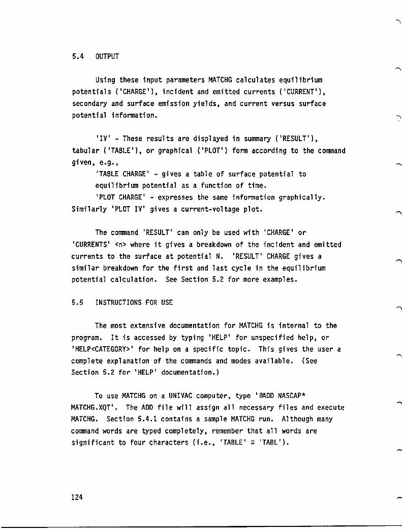
5.4 OUTPUT
Using these input parameters MATCHG calculates equilibrium potentials ('CHARGE'), incident and emitted currents ('CURRENT'), secondary and surface emission yields, and current versus surface potential information.
'IV' - These results are displayed in summary ('RESULT'), tabular ('TABLE'), or graphical ('PLOT') form according to the command given, e.g.,
'TABLE CHARGE' - gives a table of surface potential to equilibrium potential as a function of time. 'PLOT CHARGE' - expresses the same information graphically.
Similarly 'PLOT IV' gives a current-voltage plot.
The command 'RESULT' can only be used with 'CHARGE' or 'CURRENTS' <n> where it gives a breakdown of the incident and emitted currents to the surface at potential N. 'RESULT' CHARGE gives a similar breakdown for the first and last cycle in the equilibrium potential calculation. See Section 5.2 for more examples.
5.S INSTRUCTIONS FOR USE
The most extensive documentation for MATCHG is internal to the program. It is accessed by typing 'HELP' for unspecified help, or 'HELP<CATEGORY>, for help on a specific topic. This gives the user a complete explanation of the commands and modes available. (See Section 5.2 for 'HELP' documentation.)
To use MATCHG on a UNIVAC computer, type '@ADD NASCAP* MATCHG.XQT'. The ADD file will assign all necessary files and execute MATCHG. Section 5.4.1 contains a sample MATCHG run. Although many command words are typed completely, remember that all words are significant to four characters (i.e., 'TABLE I = 'TABL').
124

5.6 MATCHG Test Run
_ELCOM~ TO '~4TCHG', A ~4T~~IAL CHARGIN3 pqOGRA~. TYPE 'HELP' AT ANY TIME FOR ~SSISTANCE.
MATERIAL IS KAPT ~NVIRO~MENT NOW SI~GLE M~X~ELLIA~
PAIHMETERS
"'ATEPIAL IS -<APT. E'1ISSIO~ FO>?"'ULATIO~ IS ANGL • V9ACK = • CO KEV VINIT = .CO KEV VBEGIN = .CO I<EV vE~D = -5.GC!+~CC I<EV ANGULAR DIS TIU a UTION IS I S:)T>?OD Ie ::NVIRONMENT IS A SINGLE -"AX~~LLIAN
ELECTRO~S: NEl = 1.CO+UJ6 (~~*-3)
IONS NIl - 1.CO+:Cb (~**-3)
LIST PPOP ALL
MATERIAL = KAPT.
PROPERTY 1 DIELECT~IC CChSTANT 2 THICKNESS ! CO~GUCTIVITY
4 ATO~IC NUMBER 5 CELTA ~Ax>COEFF
6 E-~AX )OEPTH**-1 7 'H~GE 8 ExDO~ENT> qANGE 9 RANGE> EXPONENT
10 EXPONENT 11 YIELD FOq l~EV P~OTONS
12 ~AX DE/OX FOR pqOTONS 13 PHOTOCURqE~T
14 suqFACE qESISTIVITY
LIST ENVI
E~VIPON'1ENT IS A SI~GLE ~~XWELLIAN
ELECTRONS: NEI = 1.~Q+aj6 (~**-3J IONS : NIl - 1.C:J+GJ6 (~~*-3J
:HAN nlvI TEl 5.
ENVIPON~ENT IS A SINGLE ~Ax~~LLIAN
ELECTRONS: NEl = 1.~C+~~6 (~**-3J
IONS : NIl = 1.~1+a~b (~**-3J
TEl = TIl -
I.COO KEV 1.::0 KEV
I"lPUT VALUE 3.sr+:JOo 1.27-C'C4 1.::-016 5.~C+C:':O
2.1C+Ct.O 1.~C-r.Cl 7d5+CGl b.:O-C:I ~.12+::C2 1.77+("1:;0 4.5~-C'~1 1.4C+C:2 2.C(!-~GS
1.nC+C16
TEl = TIl -
TE: = TIl =
(NONE) "'ETERS MHO/M (~ONE)
("lONE) KEV A~G. ("JONE) ANG. ( N 0 ~JE ) (NONE) KEV A/"'**2 OH~S
1.C:J;J I<EV l.cao K::V
s.coo KEV 1.O:Ja KEY
COGE VALUE 3.S0+0:0 ("'ONE) 1.27-C:4 "'::SH 1.:~-O16 MHO/M 5.cc+~ac (~ONE)
4.06+C:Jl (~O~E)
8.74-:32 MIG-eH 4.29+G~1 A~G.
5.S2+CC2 A'IG. 6.eO-OCl (~O~E)
1.77+0:0 ('.jQ~EJ
4.55-fl:n (~O~E)
1.4C+CJ2 K::V 2. m:-ocs ,4//04"'*2 8.85+0:4 V-S/O
125

CHAN ENVI TIl 5.
ENVIRON~ENT IS A SINGLE ~AxwELLIAN
ELECTRO~S: ~El = 1.Ca+a~6 1~**-3) IONS : NIl = 1.CO+Juo (W~*-3)
TABLE ALL
126
TEl = TIl =
5.Q~C KEV S.CCO KEV

TABLE GENEq~T::D USING ISOT=<OPIC INCIDENT FLUX
ENEqGY n<EV) EL. SEC. EL. BKSCAT. PD • SEC. .100 2.484 • H:S .'136 .2JO 3.153 .230 .)51 .:!:JC 3.('33 .262 .~62 .4:]1: 2.742 .282 .J72 .5~O 2.460 .296 .'19C .6:JO 2.219 .307 .144 • nil:! 2.1:19 .315 .2t!1 .800 1.852 .322 .260
1.CJO 1.592 .333 .375 Z.COC .965 .316 .865 3.CDr .712 .302 1.236 4.COO .573 .29~ 1.535 S.CCO .483 .28~ 1.787 6.CJ!l .420 .272 2.~C7 7.:0C .374 .265 Z.2:Z S.COC .338 .2SQ 2.:H8 9.C:;t; .3~8 .254 2.538
lC'.0:30 .2B5 .25C 2.~86
2o.ceo .167 .234 3.561 30.COO .122 .232 4 .1~5 l&C.CJC .C98 .232 4.476 5C.COC .C83 .232 4.741
PLOT SECO
127

4.CC+CCC+ 1 I I I •
3.CO+:lCO« I >II
• I 1*
2.CQ+cnc+'IO I« I>I< I I I
1.CO+CCC+ « I I « I >11>11>11
I **>11>11
I • • • DG .e(l
*---------+---------+---------+--------+---------*---------+
PLOT BACK
128
1.~O+OQl 2.:~+JCl 3.0:+0:1 4.~G+uJl 5.0C+QOl 6.0J+JOl YIELD (FqACTION) VS. ENEf?GY (KEV)
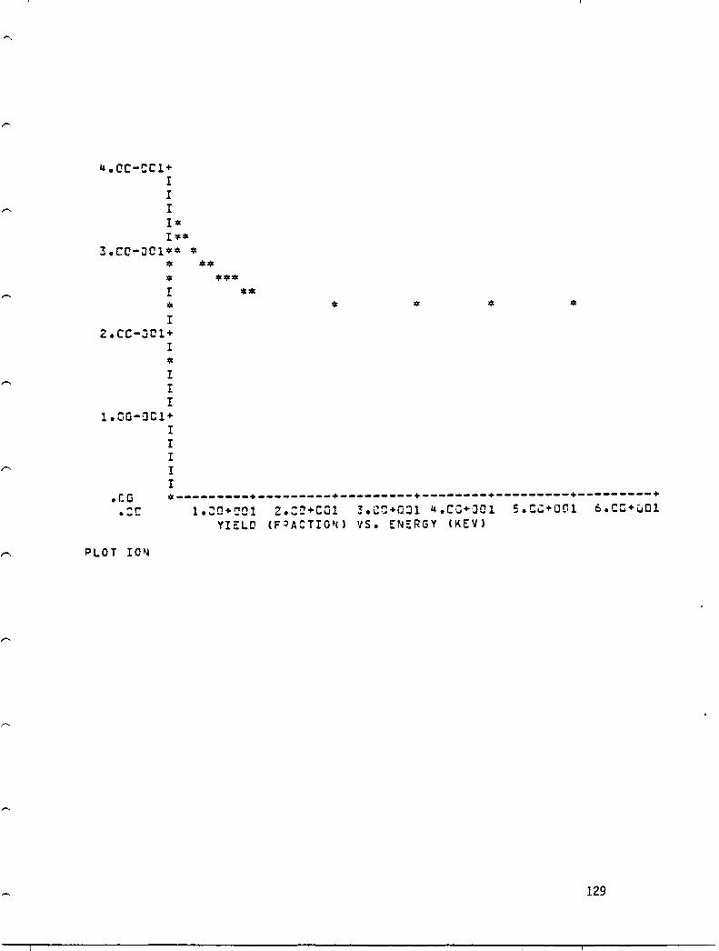
4.crC-CC1+ I I I I* I"''''
3.CC-JC1"'''' '"
'" "'''' '" "''''''' I "'* '" I
2.CC-JC1+ I
'" I I I
1.CO-aCl+ I I I I I
'" '"
.co *---------+---------+---------+--------+---------+---------+ .:c 1.:O+~Ol 2.:~+COl 3.c~+a~1 4.CC+JOl s.c~+ar.l 6.CC+uOl
YIELD (F~ACTIO~) vs. EN:;RGY (KEV)
PLOT IC~
129

s.co+ot:o+ I I I I
4.CC+:JCC+ I I I I
3.(0+010+ I ... ... T ...
2.C(j+OCC+ I I I I
1.CC+;jCC'"
>00
>00>01
>00
>01
>01
.re *---------+---------+---------+--------+---------+---------+ .ce 1.Ja+~Cl 2.C~+CCl 3.:C+CJl 4.ca+O~1 5.CO+QCl 6.0J+OCl
YIELD (F~ACTION) VS. EN::RGY (KEV)
QESULT CHARGE:
CYCLE 1 TI~:: • .:c SECONDS POTENTIAL
>Oo>Oo>OlTI~E LEFT =131013 SECONDS>Oo>Oo>Oo
I~CIDENT ELECTPON CURRE~r SECONDARY ELECT~CNS BACKSCATTERED ELECTqONS
I~CIDENT pqCTON CU~RENT
SECONDARY ELECT~ONS aUL~ CONDUCTIVITY CUR~E~T
-1.9~-C=6 8.l3-IJC7 5.;JC-C':7 u.u3-C08 1.~s-a'J7
.:'0
NET CUQQENT -4.37-~:7 A~PS/~*>Oo2
VOLTS
CYCLE 79 TI~E Z.74+aC4 SECO~DS POTE~TIAL -!.;4+003 VOLTS
>Oo>Ol>OlTIME LEFT =13C997 SECONDS>Oo*~
INCIDENT ELECToON CURRENT SECONOAQy ELECT~ONS eACKSCATTERE~ ELECTRO~S
INCIDENT PqOTON CURRENT SECO~OARY ELECT~O~S
BULK CO~OUCTIVITY CuRqE~T
130
-9.17-CC7 3.92-C':7 2.'+2-:]07 7.65-C08 2. C4-C~J7 1.a7-C:9

TABLE CHi\PGE
***TI~E LEFT =13J982 SECONOS~**
T (SEC) V (VOLTS)
-~~~~--------------------------------------.co .C'~ -4.37-:r:n S.S9+(JQ2 -E!.Cl+~u2 -3.24-:C7 1.12+~C3 -!.41+:J:!3 -2."6-J07 1.68+QC3 -1.87+~C3 -1.9G-:3Q7 2.23+:103 -2.23+0!J3 -1."s-:n7 2.79+303 -2.51+:::13 -1.17-_w7 3.35+Q03 -2.74+C~3 -9.Z2-G08 3.91+0Q3 -2.92+:~3 -7.33-:~S
4."7+J03 -3.~:'+::J3 -5.B5-:CS 5.03+Q03 -3.17+CJ3 -".be-Gee 5.59+CC!3 -3.26+C:l! -3.76-GC8 6.14+J03 -3.34+C:3 -3.C2-JC8 6.7C+C03 -!."')+0:3 -2.43-coa 7.26+:)03 -3.44+~J3 -1.96-~C8
7.82+003 -3.48+::73 -1.58-JC8 8.38+J~3 -3.51+:'J3 -1.27-G1:8 8.94+:03' -3.5l.J+J:! -1.J3-JCa 9.5C+OC!3 -3.:&+:):33 -8.29-L:C9 1.Cl+O:;4 -3.57+:JJ3 -6.7G-Gr.9 1.Cb+(J04 -3.59+J:j:! -S.41-:C9 1.12+0~4 -3.6:+J::13 -".37-:C9 1.17+0Cu -3.61+0:3 -3.S3-:!J9 1.23+JC4 -3.61+0J3 -2.86-~li9 1.Z8+JQ4 -3.62+.1:!3 -2.31-Q:9 1.34+QC4 -3.62+')1:3 -1.87-:C9 1.40+0C4 -3.63+0:3 -1.51-:09 1.'+s+ao'+ -3.63+::!~3 -1.22-:09 1.Sl+u04 -3.63+:33 -9.88-:10 1.56+0C4 -3.63+'J::! -g.C'O-Cl~
1.62+004 -3.63+J~3 -6.47-JlC 1.68+004 -!. 64 +C:)3 -5.23- Jl: 1.73+QC4 -3.6~+::3 -4.23-:n: 1.79+004 -3.64+a:J3 -3.42-J!: 1.84+u~4 -3.64+':~3 -2.77-:'1: 1.90+:JC4 -3.64+J:=:; -2.Z4-:1!J 1.95+C(!4 -3.64+::3 -1.81-.110 Z.01+004 -3.64+J:3 -1.47-:J1G 2.07+Q04 -3.64+::)3 -1.19-:1: Z.12+QC4 -3.64+~:3 -9.59-:11
131

PLOT CHARGE
~~*TIME LEFT =13G981 SECONDS~**
***TIME LEFT =130966 SECONDS~**
132
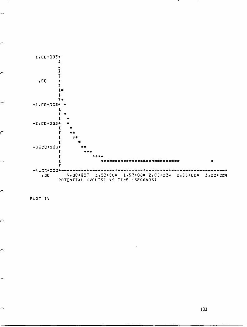
r
1.CO+003+ I I I I
.CC * I I. I 1*
-1.CO+~C3+ * I I * I *
-2.ro+uQ3+ I I I r
-3.CC+~03+
I I I I
**** ********* •••• *****.**.** •• *. *
-4.~C+:03+---------+---------+---------+--------+---------+---------+ .oc ~.Qa+aC3 1.~C+OQ~ 1.5~+CU4 2.0:+CC4 2.5~+OG4 3.C~+=C4
POTENTIAL (VOLTS) VS TII"E (SECOf\jOS)
PLOT IV
133

2.CiC-~07+
I I
1.C:-J07+ * I :0<
I * I * * +
I I
-1.0C-ilC7+ I I I
-2.0G-C~7+
I I
-3.CQ-~C7+ I I r
-tl.CC-D01+ I I
>I< *
-5.QG-~C1+---------+---------+---------+--------+---------+---------+ -S.CC+CO: -4.~~+~OC -3.;O+OCC -2.CC+CJO-l.rO+G~C
CURqE~T (AMPS) VS. VOL TAGE (KEV'
TABLE IV
134
1.OQ+Q:J:J

r v JTOT JE JSECE JBSCAT .C~ -4. :!7-0c:'1 -1.9J-~06 9.13-C07 5.C:-0O1
-2.38-uCl -Il. GZ-O~17 -1.31-0:6 7.75-CC7 4.71-J01 -4.76-C!H -3.68-Q07 -1.73-QC6 7.39-CC7 4.55-001 -7.14-:J01 -3.36-0:J7 -1.&5-006 7.~S-007 4.34-001 -9.S2-~Q1 -:!.C4-CC7 -1.57-C~6 6.72-CG7 4.14-CIJ7 -1.19+'JCC -2.73-001 -1.50-0:6 6.41-C~7 3.94-:07 -1.Il3+QCC -2.Ll3-0C7 -1.43-a~6 6.11-C::J1 !.76-::J7 -1.67+0CO -2.14-a~7 -1.36-006 5.82-Q:]7 3.S9-C07 -1.9[3+COO -1.86 -C07 -1.30-GC6 5.5S-C~1 3.42-C07 -2.14+000 -1.58-0!:!1 -1.24-0~6 5.30-007 ! .26-0~17 -2.38+000 -1.31-Q07 -1.18-0C6 s.aS-G07 3.11-0:)7 -2.62+0(1: -l.eS-007 -1.13-006 4.81-:C7 2.96-iJ07 -,.86+000 -7.97-008 -1.~7-0:b 4.S9-C01 2.83-CC7 -!.1C+QCO -5.48-0C8 -1.~2-(jab 4.38-007 2.69-C07 -3.33+GC~ -!.C5-0:l8 -9.75-0:7 4.17-:n7 ~.57-~~7 -3.S7+QCC -~.96-::JJ9 -9.!O-:C7 3.Q8-:a7 2.45-:JJ7 -3.81+CC: 1.63-C:8 -8.97-C:H 3.79-CC7 2.34-G07 -4.CS+QOC 3.89-CQ8 -8.45-J::!7 3.&2-C::J7 2.23-0n7 -4.29+:CG 6.11-0C8 -8.J6-JC'7 3.45-QQ7 Z.12-C07 -tl.52+~r:!C 8.27-:JC8 -7.69-C!::7 3.29-G07 2.t:'3-:~7 -4.76+000 1.04-0C7 -7.!3-0::7 3.14-':C7 1.93-!JCn
RESULT CURRENT -Z.:7C
CUR~E~TS FOR POT~~TIAL OF -2.:7+CJO KV
INCIDENT ELECTPON CURRENT -1.26-CC6 SECO~DA~Y ELECT~O~S 5.37-C:7 BACKSCATTERED ELE=T~ONS 3.31-CC7
I~CIDENT PQOTON CUqRENT 6.26-0:8 SECONDAQy ELECT~O~S 1.S7-CC7
BULK CONDUCTIVITY CURRENT 1.63-CC9
CHANGE ENVI DIRECT 9
DATA IN FILE IS FqO~ S9~:G SECO~OS ON DAY 87, 199G TO 59JJa S~CONDS ON DAY 87. 19Bu
SPECTqA FQUND FOP 59can SECC~DS ON DAY 87, 199C 09JECT POTENTIAL = -2C:~.~ VOLTS SINGLE ~O~ENT FIT 3IVES ~l= 9846Jl. T1= 5111.78 SINGLE ~O~ENT FIT ~IVES ~l= .l=a257+~C7 T1= 511~.89
APPPOXI~ATE DENSITIES AND TE~PE~ATURES:
JI JSECI 4.43-0C'8 1.~S-:C7 4.54-Dca 1.1::-007 4.85-:08 1.15-007 5.06-008 1.21-007 5.27-C08 1.27-~C7 S.48-G08 1.33-:07 5.70-0C8 1.39-007 5.9:'-C08 1.46-:)07 6.12-008 1.52-007 6.33-008 1.59-007 6.54-008 l.b6-0C7 6.75-008 l.73-'JC7 5.96-QC8 I.BO-OC7 7.17-008 1.87-Q07 7.38-1)08 1.9Q-CC7 7.59-0(;8 2.ttl-CC7 7.se-J08 2.C9-a07 8.£:'1-0:)8 Z.17-JC7 8.22-0C8 2.24-0C7 8.43-QC8 2.32-007 8.64-GC8 2.40-C07
135

136
SPECrE: l( -1) 2 ( 1)
TABLE ALL
DE"lSITYP'-3) 9.85+CQS 1.O'+C06
TEMPlEv) 5.11+;::C3 5.1!.+CC3
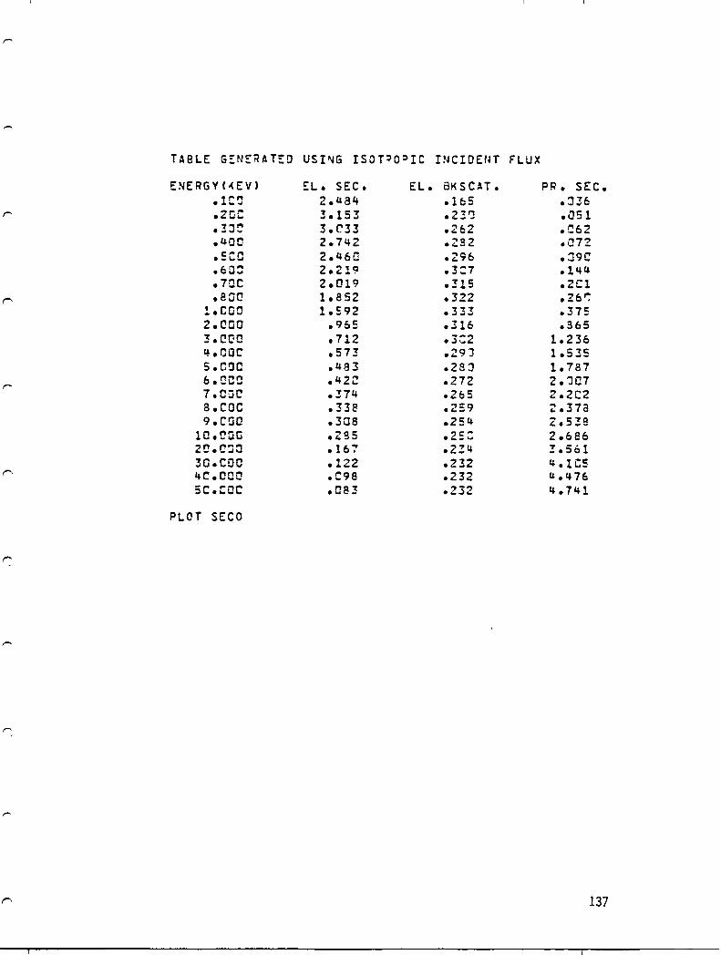
TABLE G~NERAT::D USI~G ISOT~O:::lIC INCIDENT FLUX
ENERGY(.(EV) ::L. SEC. EL. 8KSCAT. PRe SEC. .1Ce 2."34 .1E;S .J3& .ZOC 3.153 .2!'J .0Sl .!:J~ 3.C'.'33 .262 .~62 ."00 2.742 .282 .072 .sec 2.46e .296 .~9C .60:: 2.219 .3:7 .144 .7QC 2.Q19 .!15 .2e1 .80Q 1.852 .322 .Z6r;
!.CQO 1.592 .333 .375 2.COO .965 .316 .965 3.CC:O .712 .3<::2 1.236 4.COC .573 .29) 1.535 5.000 .483 .28:) 1.787 6.eCe .42C .272 2.jC7 7.CDC .374 .265 2.2C2 B.COC .338 .259 2.37a 9.C(jQ .308 .254 2.538
lO.COG .2SS .25: 2.68b 'D.C:):) .16i .2ZIt 3.561 30.COO .122 .232 ".1 C5 4C.CCO .1:98 .232 U." 76 SC.COC .083 .232 4.741
PLOT SEea
I"" -
137

4.CO+:JCQ+ I I r I >01
3.0Q+OCC* 1
• * I 1*
2.CQ+Jec+* I>Cl II I I
1.CC+CCC+ * I
I * I * •• I",,,,,,,. I '" .co .---------+---------+------___ + ________ + _________ ~----_____ +
.CC 1.00+001 2.JO+O~! 3.aO+aCl u.a~+Ga1 s.o:+n01 6.0Q+001 YI~LD (F=?ACTION) VS. EN::RGY (KEV)
PLCT BACK
138

4.CG-OC1+ I I I I* I*'"
3 .CC-OtH** * * "'''' * ."'''' I "'''' * * I
2. CG-:(H + I
* ,- I ... .£.
I 1.CO-JC1+
I I r I I
.~o *---------+---------+---------+--------+---------+---------+ .ot' 1.JC+~~1 2.J~+=Cl 3.:0+a~1 u.rC+CJl S.O:+GCl 6.CO+~Ol
YIELD (F~~CTION) vs. EN::RGY (KEV)
PLOT IO~
139

5.CC+:JCC+ I I I I
4.CG+;)CC+ I I r I
3.CO+OOC+ I I I
2.1:0+000+ I r I ".
I * 1.CC+~CO+
I * I
'-
.ro «---------+---------+---------+-----~--+---------+---------+ .CD 1.uC+COl 2.0C+OQ1 3.0Q+Q~1 4.c~+cal S.OC+GDl 6.CQ+OCl
YI::LD (F~ACTICNJ VS. EN::RGY (KEV)
RESULT CHAQGE
CYCLE 1 TIME .oc SECONDS POTENTI.AL
***TI~E LEFT =13~9S8 SECONOS***
I~CIOENT ELECTQON CURQENT SECO~DA~Y EL~CTQO~S SACKSCATTEQED ELECTqO~S
INCIDENT PQOTON CUqRENT SECONDARY ELECTQO~S
BULK CO~DUCTIVITY CURRE~T
-!.a8-t'C6 8.27-:G7 4.93-:::7 4.42-0:8 1.C4-!:'C7 .J~
--------------
.:0
~ET CURqENT -4.:9-~:7 A~PS/~**2
VOLTS
CYCLE 72 TI~E 2.98+::4 SECONDS POTENTIAL -3.49+0Q3 VOLTS
I~CIDENT ELECTRON C~RqE~T SECONDARY ELECT~ONS SACKSCATTERED ELECT~ONS
r~CIDENT pqOTO~ CUQRENT SECONDAQY ELECTQC~S
BULK CONDUCTIVITY CURRE~T
140
-9.!OS-CC7 4.l9-':'~7 Z.S~-CC7 7.49-CC8 1.98-C:7 2.74-'::'09
--------------

TABLE CHARGE
••• TIME LEFT =130948 SECONOS~ ••
••• TIME LEFT =130938 SECONJS***
T (SEC) V (VOLTS'
.CC .1:0 -u.09-:C7 6.09+:)02 -9.C9+~J2 -2.99-:07 1.;:Z+J03 -1.41+0J3 -2.21+-:07 1.83+:103 -1.87+0a3 -1.7C-OC7 2.44+:303 -2.21+C~3 -1.31-C:7 3.C=+~C3 -2.4B+:~3 -1. :1l-CC7 3.65+:C3 -2.69+J:i! -7.a7-:08 4.'&+C03 -2.86+:"3 -6.14-:Ca 4.87+~O3 -2.99+:):3 -4.S4-CCe 5. u 8+)03 -3.C9+Q:3 -3.82-':'C8 6.C9+J03 -3.17+J03 -3.C2-GC€ 6.7C+J03 -3.23+~=3 -2.UG-JC8 7.31+:103 -3.28+::1:: -1.9J-JOS 7.92+::;:3 -3.32+:::33 -l.5l-COS 8.53+003 -3.35+::33 -1.Zl-J'J8 9.14+;JC3 -3.33+:J3 -9.6C-:C9 9.75+:}03 -3.4D+·)03 -7.65-JC9 1.C4+JC4 -3.42+:J~3 -6.1';-009 1.10+JC4 -3.43+J:3 -4.S6-~~9
1.16+004 -3.U4+;:J3 -3. a 8-'~C9 1.22+:04 -3.4S+:J! -3.C9-CI:9 1.2S+JC4 -3.45+:)1)3 -2.47-':C9 1.34+:)C4 -3. u b+:J3 -1.97-:09 1.40+004 -3.46+003 -!.S7-~C9
1.46+::304 -3.47+::3 -1.2S-0G9 1.~2+a(l4 -3.47+):33 -1.CC-C09 1.58+::304 -3.47+:J03 -7.98-:1C 1.64+CC4 -3.47+CJ3 -6.37-G1C 1.71+QC4 -3.47+IjC3 -5.:38-C1: 1.71+004 -3.47+=03 -4.Cb-:J1~ 1.83+J04 -3.49+0:!! -3.24-:1C 1.89+JC4 -~.4a+J:J3 -2.58-:10 1.95+JC4 -3.43+J:! -2.Cb-C1G 2.Cl+:JC4 -!.48+'J~3 -1.bS-':1~
2.C7+QC4 -3.48+J~3 -1.31-::1;: 2.13+CCu -3.49+:::3 -1.~S-~la
PLOT CHAQGE:
141

* •• TI~E LEFT =13~938 SECONDS***
••• TIME LEFT =13C927 SEC~~DS***
142

1.r.O+:J03+ I I I I
.CO ~
I I* I I*
-1.00·003+ * I
I '* I *
-2.aa+C'~3+ * I ~* I * I ** I **
-!.CD+J03+ *** I **** I ***************************** I I
*
-4.c~+aa3+---------+---------+---------+--------+--~------+--------~+ .CD S.OO+~C3 1.~~+CC4 :.50+u04 2.:C+cr~q 2.5C+GCq 3.3Q+QOQ
POTENTIAL (VOLTS> VS TI~E (SECONDS)
PLO T I V
143

2.CO-J07+ I I
1.OG-!J01+ *' I*'*'
.cc I *' I *' +
I I
-1.CO-007+ I I I
-2.:-C-aC7+ I I
-3.r:c-:r7+ r I I
-4.CC-JC7+ I I
*' *'
*'
*' '"
-5.=0-037+---------+---------+---------+--------+---------+---------+ -S.OC+CC: -4.CO+OJC -3.:0+cac -2.CC+1:J-l.~C+G:: .co l.a~+co~
CURP~ ... T (AMPS) VS. VOLTAGE (KEV)
TABLE IV
144
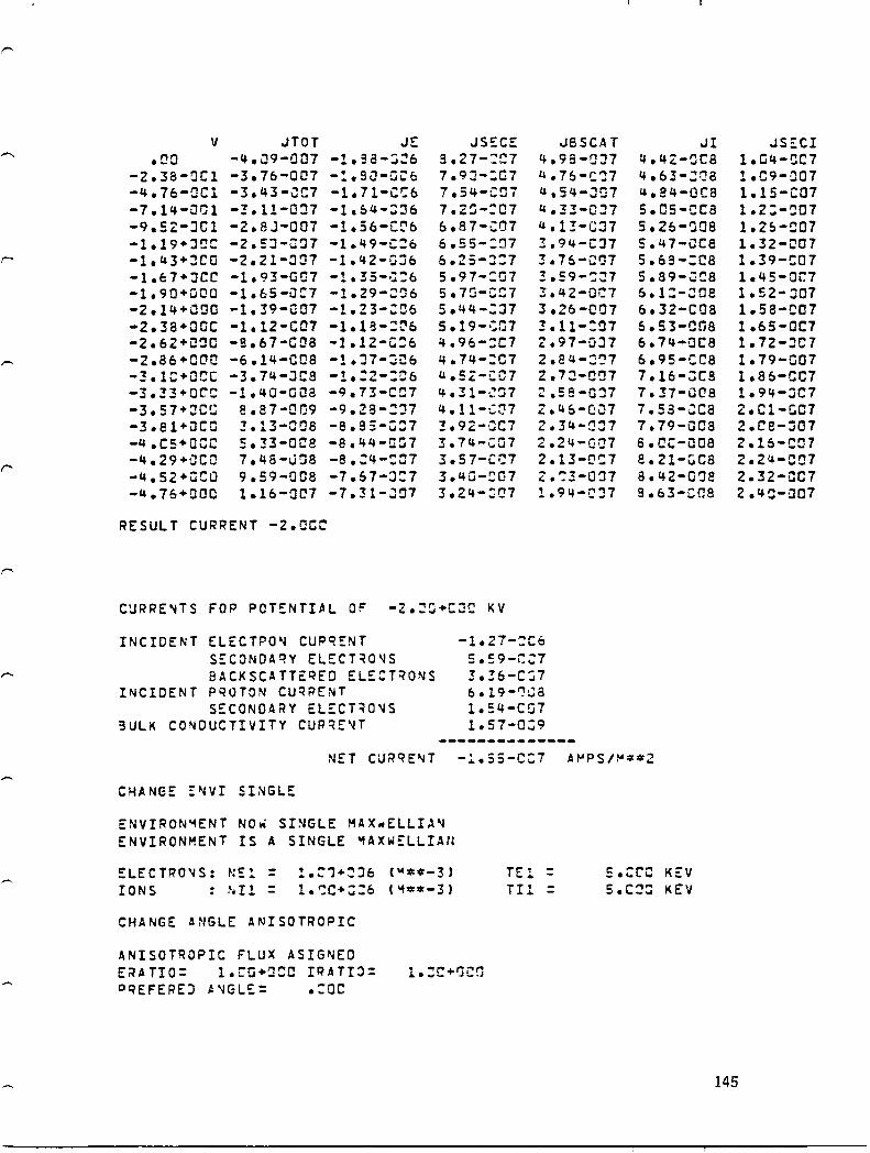
r-
v JTOT JE JS~CE ..IBSCAT .ao -4.;:)9-Q07 -1.3a-::i~6 3.27-:rn 4.98-0J7
-2.38-0Cl -3.76-0(:17 -:.9O-GC!: 7.9J-::G7 u.76-C'J7 -4.76-aCl -3.43-~C7 -1.71-C':6 7.54-C!Ji U.54-J!;7 -7.14-0Cl -!.ll-O:17 -1.&4-:J:J6 7.2!j-:07 u.33-0J7 -9.52-:]01 -Z.8J-007 -1.56-C!:'b 6.87-:: rJ7 4.13-(;:37 -l.l9+::l0C -2.:::1-0:17 -1.49-C:o 6. SS-:~'17 !.94-CJ7 -1.43+~C(J -2.21-0:n -1.42-0:16 6.25-::7 3.76-Cr:J7 -1.E:7+JCC -1.93-007 -1. 35-·~:6 5.97-:07 3.59-:~7
-1.90+000 -1.65 -a~7 -1.29-::;'J6 5.7G-CC7 3.42-0C7 -2.l4+C!J0 -1.39-CQ7 -1.23-:06 5.44-::)7 3.26-C07 -2.38+00C -1.12-C07 -l.18-:t'6 5.19-·:07 :3 .11-:07 -2.62+000 -S.67-CD8 -I.12-C:6 4.96-:C7 Z.97-0J7 -2.86+QL'C -6.14-008 -1.J7-~;:6 4.74-:07 2.S4-:~7
-3.1C+QCC -3.74-JC3 -1.:Z-:06 u.5Z-CC7 2.7;:!-C'.J7 -3.!3+QCC -1.40-008 -9.73-CC7 4.31-·:~J7 2.S8-a~7
-3.S7+:!CG e .87-0 D9 -9.28-::)7 4.!l-:::::t7 2.46-(;07 -3.al+uCO 3.13-008 -8.S5-u:n !.92-CC7 2.34-!J:n -4. CS+QCC 5.!3-0C8 -8.44-Q:n 3.74-C07 2.24-aa7 -4.29+uCO 7.48-J08 -8.:4-:07 3.S7-CC7 2.13-£:'=7 -4.sz+uca 9.59-008 -7.57-:):7 3.4D-:07 2. ~3-a~)7 -4.76+000 1.1b-QC7 -7.H-J07 3.24-:;07 1.94-CJ7
RESULT CURRENT -2.QCC
C~RRE~TS FOP POTENTI~L OF -2.:a+c~c KV
INCIDENT ELECTPO~ CUPQENT -1.27-:C6 SECONDAQY ELECT~O~S eACKscATT~qED ELS:T~O~S
INCIDENT P~OTON CU~PENT SECONDARY EL~CT~O~S
3ULK CO~DUCTIVITY CUPRE~T
CHANGE ~~VI SINGLE
ENVIRON~ENT NO. SI~GLE MAX~ELLIA~
ENVIRONMENT IS A SINGLE ~AX~~LLIAN
S.=9-~':7 !.36-C:7 b.19-~Ga
1.54-CG7 1.57-0:;9
..II 4.4Z-0ca 4.63-:0a 4.84-01:8 s.cs-cce 5.26-')08 S.47-CCB 5.69-:C8 5.89-~C8 6.1:-::;08 6.32-CD8 6.53-008 6.74-QC8 6.95-CC8 7.16-3C3 7.37-0(18 7.58-.:ca 7.79-008 8.CC-QOa S.21-GC8 8.42-0':]8 a.b3-ce8
ELECTRO'S: NE! = :.:1+:l6 (W~~-3)
IONS : ~Il = 1.~C+~:6 (~**-3) TE 1 = TIl =
S.:C'C KEV S.C~: KEV
CHANGE ANGLE ANISOTROPIC
ANISOTROPIC FLUX ASIGNED ERATIO= 1.rG+~:0 I~ATI~= PQEFEREJ A~GLE= .:ac
JS::CI 1.G4-!:C7 1.C9-007 1.l5-C07 1.2:-~O7
l.Z6-C07 1.32-C07 1.39-C07 1.45-0C7 1.S2-:J07 l.5S-C07 1.65-0C7 1.72-::107 1.79-C07 1.86-CC7 1.91f-JC7 2.Cl-GC7 2.C8-007 2.15-C07 2.24-007 2.32-CC7 2.4C-:J07
145

CHANGE ANGLE EPAT J.
ERATIO: .:c IRATIO: 1.C:l+C:C
CHANGE ANGLE IqAT C •
• ::0
CHANGE ANGLE PREF 25.
PREFERED A~GLE: 2S.00~ JEG~EES
~ATERIAL IS KAPT. EHISSIO~ FORMULATION IS AN3L. V3ACK: .~D KEV VINIT: .~C KEV V3EGIN : .a~ ~EV VEND : -S.~C+~~~ KEV ANISOTP~PIC FLUX PQEFEREJ DIQECTION: 25.=C~ ~E~REES E~ATIO( 1) = .:!(' IRATIO( 1): .jC ENVIRON~ENT IS A SINGLE ~Ax~ELLIAN
ELECTRO~S: NEl : IONS NIl:
TABLE ~LL
146
1.Gr.+a~6 ("'**-3) 1.ca+:J~6 ("I>lO*-3)
TEl : TIl:
5.CC: r<EV 5.GOa KEV

TABLE G~NE~ATEO USI~G A~rSOT~OPIC INCID~NT FLUX AT 2S.:JG+QCC OE~REES
ENEqGY(KEVJ EL. SEC. EL. BKSCAT. PR • SEC. • !JC 2.484 .1&5 .:!6 .2:0 3.153 .230 .:51
"l,,'" e_.w 3.033 .262 • .362 ."ce 2.742 .282 .~72 .:00 2.460 .296 .~9C .6~Q Z.21 Cl .3::7 .1414 .7:1J 2.019 .315 .2e1 .sao 1.852 .322 .260
I.ceo 1.592 .333 .:ns 2.C~Q .965 • .316 .365 3.cac .712 .3CZ 1.2 !6 4.S0C .573 .290 1.535 5.:00 .1483 .28C 1.787 6.~OC .42C .272 2.:JG7 7.CCC .3714 .265 2.2C2 a.cae .338 .259 2.378 9.C~:J .308 .254 2.538
lo.tee .285 .25e 2.586 2C.C:JO .167 .234 3.561 3C.CCC .122 .232 ".lCS 4r..r:O: .098 .232 ".476 5(,.00C .Cs! .23= 4.741
RESULT CHAPGE
CYCLE 1 TI"1E SECONDS POT~NTIAL VOLTS
***TI~E LEFT =13:922 SECONDS***
INCIDENT ELECTRC~ CUPqE~T -1.9~-C:6
SECONDAqy ELECT~O~S B.l3-ce7 2ACKSCATTEPED ELECTRO~S S.~G-C:7
I~CIDENT PQCTQN CU~RENT 4.43-C:8 SECO~DA~Y ELECT~O~S 1.:S-C:7
aUL~ CO~DUCT!VITY CURRENT .:0
NET CUR~E~T -4.37-~C7 A~PS/~**2
CYCLE 78 TI~E 2.74+:C4 SECONDS POTE~TIAL -3.64+JC3 VOLTS
***TI~E LEFT =13c9nz SECO~OS***
I~CIDENT ~L£CToO~ CURRE~T -9.17-C~7 SECONOA~Y ELECT~ONS !.Cl2-C07 ~~CKSCATTERED ELECT~O~S 2.42-~07
I~CIOENT P~OTON CUQRE~T 7.bs-c:a SECONDARY ELECT~O~S 2.:4-C: 7
3ULK CO~OUCTIvITY CURRE~T 2.87-:C9
PLOT IV
147
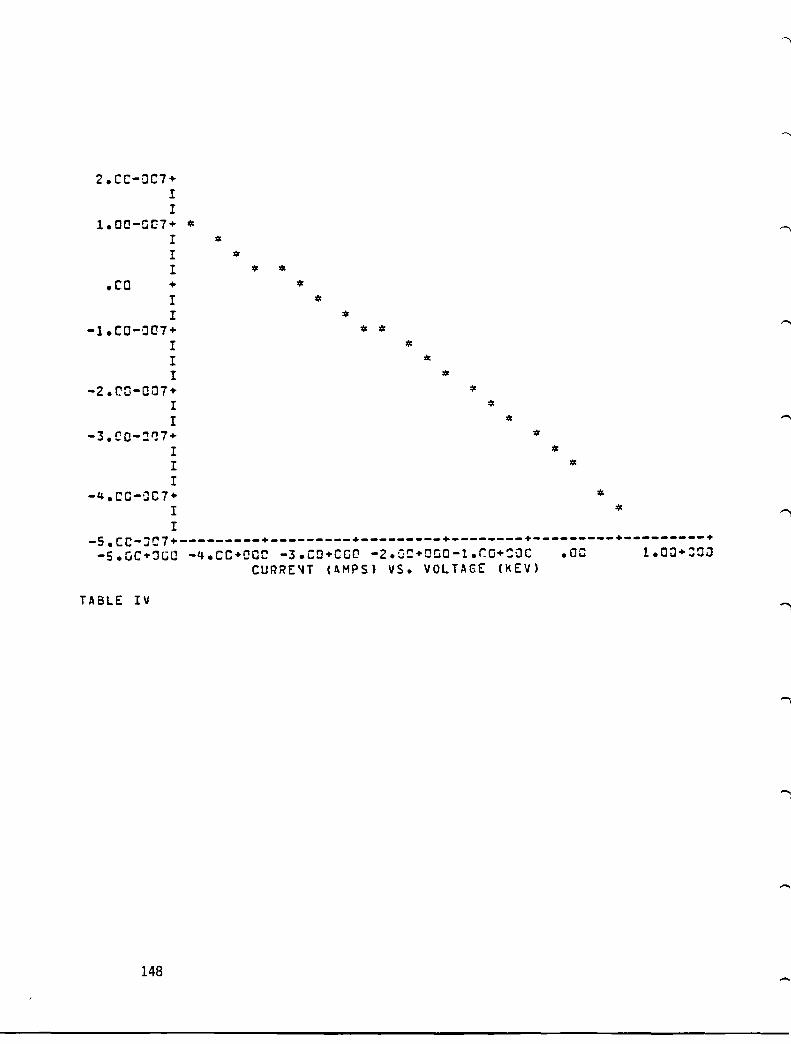
2.CC-OC1+ I I
1.00-001+ '"
.co
r >I<
I >I<
I >I< >I<
+ I I
-1.CO-QC!1+ I I I
-2.('Q-007+ I I
-3.CQ-::!"7+ I I I
-4.CC-JC1+ I r
>I<
>I<
>I< >I<
>II:
-S.CC-3C7+---------+---------+---------+--------+---------+---------+ -S.Gc+~Ga -4.CC+QCC -3.CO+CG~ -2.GC+OGO-l.CO+:OC
CURRE~T (~MPS) vs. VOLTAGE (KEV)
TABLE IV
148
.oc 1.0;:)+:::00

.--
V JTOT JE JSECE J8SCAT .CO -4.37-0~7 -1.9C-S:b 8.13-CC7 S.C,]-GJ7
-2.38-:lCl -4.C2-QC7 -1.81-G:!b 7.75-0~7 4.77-C07 -4.76-JOl -3.68-::C7 -1.73-Q:6 7.39-1J!:7 u.55-J~7
-7.14-.;r1 -3.3b-CC7 -1.55-COb 7.C!S-GC7 u.34-::(37 -9.52-:01 -3.C4-UC7 -1.57-CCc 6.72-C':7 4.14-':07 -1.19+:JGC -2.73-CJ7 -1.SC-:::6 6.41-':C7 3.94-:~7
-1.43+QOC -2.43-007 -1.43-C06 6 .1l-C~j7 3.76-G0)7 -1.67+~a: -2.14-u07 -1.3b-:;:b 5.32-C:7 3.S9-JJ7 -1.90+0CC -1.86-007 -1.3:-CC6 5.55-GC7 3.42-C07 -2.14+;JCO -1.58-J:J7 -1.24-C:J6 S.30-0C7 ?26-J07 -2.39+:lCC -1.31-;J:7 -1.18-CJ6 s.:s-aC7 3.11-0~7 -2.62+0:!G -1.CS-OC7 -1.13-0:16 4.81-':::7 2.96-::;7 -2.86+~'=C -7.97-0ca -1. :17-I:::1b 4.S9-c:n 2.83-';07 -3.1C+:OC -5.4a-ocs -l.:lZ-OC!b 4.38-C:::7 2.69-c:n -3.33+~OG -3.:5-0C" -9.75-0:7 u.17-;:C7 2.57-~:7
-3.57+:::01'1 -6.8b-J:l9 -9.3C-G~1 3.98-CG7 2.1J5-CJ1 -3.81+JOC 1.53-COS -S.37-J:!7 3.79-C':1 2.34-:07 -IJ.CS+:CG 3.89-0:8 -8.4S-UC7 3.62-GC7 2.23-c:n -4.29+:0: 6.11-J:a -8.J6-CC7 3.45-":C7 Z.12-G07 -4.52+3CC 8.21-QCB -7.&9-::17 3.29-;:;:7 2."':!-:~7
-4.76+:CC 1.G4-007 -7.33-:3::17 3.14-C:~7 1.93-CJ7
RESULT CURPPIT -2.j7Q
CURRENTS Foe POTENTI~L OF -2.J7+GC: KV
INCIDENT ELECTRON CUPqE~T
SECONDARY ELECTqO~S oACKSCATT~~ED ~LE:T~C~S
INCIDENT PQOTON CUqRE~T
S~CONDAgy EL~CT~C~S
SULK CONDUCTIVITY CUPRE~T
CHA~GE A~GLE ERAT 1.E4
(RATIO= 1.::0+,:)04 IRATI:>=
CHANGE ANGLE IRAT 1.E4
ERA TIO=
CHANGE ANGLE PREF O •
pqEFEREJ A"lGLE= • C':C :lE3REES
LIST ENVI
5.37-:::7 ~.;1-:C7
o.2c-Ci;s:! 1.57-C'J7 1.c3-C.J9
JI JS~CI u.43-GC!8 1.05-::!H 4.64-005 1.1:1-:C7 4.85-0Ca 1.15-J07 S.Cb-OtJ8 1.'1-Q07 5.27-IJC8 1.27-007 S.48-JC8 1.33-:1Q7 S.7Q-GOa 1.39-~07 S.91-008 1.46-J07 6.12-(;08 1.52-Q07 6.33-Q08 1.59-0C7 6.S4-cca 1.66-::107 5.75-~CS 1.73-jC7 6.9b-008 1.se-QC7 7.17-GC8 1.87-:lC7 7.38-L:C8 1.91J-:C7 7.59-GC8 2.01-J07 7.8G-CCB 2.09-J07 8.Cl-OC8 2.17-C07 3.22-CQ8 2.24-007 S. 43 -iJca 2.32-J07 8.64-00a '.4u-QC7
149

~NVIOON~ENT IS A SINGLE ~AX.~LLIA~
ELECTRONS: NEl = 1.CC+'J:J6 (101*""-3) IONS ~Il = 1.r:C+JJb (~""*-!)
TABLE ALL
150
TEl = TIl =
5.COC KEV S.C::;: KEV
.-.,

TABLE GE\E~ATED USING A~ISOTROPIC INCID~NT FLUX AT
ENERGY(KEV' • !OO
.3:C
.40~
.::!:1
.60'::
.70u
.SOO 1.COO 2.coa 3.aco 4.GOC :.C'jO 6.0QC
e.reo 9.CI;JC
H" .cce 20.0;JO 3(,.C~C
4C.CQC 5C.C~O
RESULT CHARGE
EL. SEC. 2.241 2.559 2.276 1.958 1.7C6 1.~13 1.362 1.241 1.050
.639 .11.72 .390 .321 .279 .Z4e .22" .2~:
.189
.111
.C32
.a65
.CS5
EL. eKSCAT. .'J93 .151 .18C .~99
.213
.224
.232
.239
.2se
.233
.2l9
.198
.19C'
.183
.173
.173
.169
.155
.152
.152
.152
PP. SEC • .::24 .034 .~41 .J48 .'J6e .J96 .134 .173 .2se .577 .824
1.~23
1.192 1.338 1.468 1.585 1.692 1.791 2.374 2.737 2.984 3.161
CYCLE 1 TIIoIE .ce SECONDS POTENTIAL
***TIME LEFT =13~e95 SECONDS***
I~CIDENT ~LECT~O~ CURQE~T
S£CONDAPY ELECT~O~S 2ACKSCATTERED ELECTRONS
I~CIDENT P~OTON CUQRE~T
SECO~DARY ELECT~ONS aULK CONDUCTIVITY CURRE~T
-2.eS-:C6 8.14-C.:7 S.!Q-":C7 6.65-0::8
.. ,. .--~ET CU~qENT -1.34-rC6 A~PS/M**2
.ec: DE3R=:ES
VOLTS
CYCLE 99 T!~E 8.89+~G3 SECO~DS POTENTIAL -6.14+C03 VOLTS
***TI~E LEFT =13087: SECONDS***
INCIOE~T ELECTRO~ CURqE~T
S~CONDARY ELECT~C~S 9AC~SCATTERED EL£CT~ONS
INCIDENT PQOTON CU~RE~T
SECONDARY ELECT~ONS BUL~ CC~OuCTIVITY CURRE~T
TABLE CYAPGE
-Q.35-JC7 2.!9-0C7 :.:Z-CC7 !..4a-~C7
2.87-:C7 4.83-:C9
151

***TI~E LEFT =13~a70 SECO~DS.**
***TI~E LEFT =130845 SECONDS***
T (SEC) V (VOLTS) I (A"'PS/"'*>lt2) -------------------------------------------.co .Co -1.34-~Cb
1.81+:)02 -8.47+-J02 -l.oa-COb 3.63+:102 -1.54+033 -8.84-~C7 5.44+;lO2 -2.11+:1J3 -7.3 O-CC7 7.26+Q!:!2 -Z.6C+JC!3 -6.27-:::i7 9.G7+:lC2 -3. (::1 +C:3 -s .37-:rn 1.('19+~03 -3.!1+~a3 -4.6!-:C7 1.27+:)::3 -3.bS+~~3 -4.C'3-::C7 1.4:;+u:3 -3.95+::l! -3.52-~C7 1.63+QC3 -4.!.9+:.J03 -3.D9-::G7 ....... 1.81+:l03 -'+.4:1+J:::3 -2.7!-Gr'!1 2.CQ+QC3 -4.5S+:03 -2. 11 1-CC7 2.18+JrJ3 -4.75+~J3 -2.l4-CC7 2.36+:)03 -4.89+C!:!3 -1.9C-':07 2.S4+:JC3 -5.C'2+::lJ3 -1.69-~rl1
2.72+~!J3 -5.14+:3:13 -l.S:'-C~7 2.90+303 -5.24+C:J! -1.35-~C7
3.08+003 -5.34+0iJ3 -1.21-;07 3.27+303 -S.1l2+JJ3 -1.::;8-0(;7 3.45+jC:! -5.49+0::3; -9.7:J-::i!:8 3.63+:103 -S.S6+C~3 -8.71-::::8 3.81+Ja~ -5.62+0::J~ -7.83-:('e 3.99+:::03 -5.67+J:J3 -7.C4-::;8 1l.17+JG3 -5.72+0:3 -6.33-:['8 4.3S+~C3 -S.76+~J3 -5.72-:~8 4.54+:::03 -s.a~+O:l3 -5.13-C:8 4.72+0C3 -5.84+C::3 -4.63-cca 4.9C+:lC3 -S.87+rJ~3 -4.17-.JCS 5.:;S+:::'3 -S.()J+C:3 -3.75-:C8 5.26+:lC3 -5.93+a~3 -3.3Q-~r8
5.44+003 -S.95+0J3 -3.C6-008 5.62+003 -S.97+~'3 -2.76-::"8 5.81+003 -5.99+~u3 -2.5C-:':8 5.99+JC3 -&.Cl+:~3 -2.25-:08 6.17+aC3 -6.02+~u3 -2.C4-Cfj2 6.35+003 -6.r4+1J3 -1.84-~ca 6.53+:;u3 -6.CS+!J:J3 -1.66-:S8 6.71+J:3 -5.C'6+~J! -!.SJ-:~8 6.89+J:3 -6.C::7+J~3 -1.!b-i:.C8 7.C8+JC3 -6.1J3+::J3 -!.23-CC8 7.26+J="3 -6.C9+::;~3 -!.ll-;JCa 7.44+CC3 -6.1:+:!~3 -1.:C-':28 7.62+QC3 -6.!J+:;Q3 -9.C7-CC9
152

7.80+J03 7.98+J03 8.1C+:)C3 S.3S+JC3 8.S3+J~3
8.71+C03 8.89+:)03
PLOT CHAI?G~
-5.11+~:J3
-5.11+0:3 -6.12+0~3 -5.12+033 -6.13+JJ3 -6.13+(;:3 -5.14+1)03
*.*TIME LEFT =13~84S SEC~NJS~**
***TIME LEFT =130821 SECONDS***
-.3.2S-:C9 -1.4:-C:9 -6.71-::i;9 -6.('17-0:9 -5.4Q-:~9
-4.9E:-GC9 -4. a 9-:iCQ
153

1.CC+OC3+ I I
* r" I
-1.CC+:)C3+* I '" I * I * I * 1 **
-3.C~+:JC3+ * I * 1 ** I * I ** I ""*
-=.CC+jC3+ *** I **** 1 ******* I ""************************ I I
-7.CC+~~~+-----------+-----------+----------+-----------+-----------+ .oc 2.~a+cc3 4.:0+~03 6.CJ+~C3 8.C;J+QC3 1.00+004 POTENTIAL (VOLTS) VS TIME (SECONDS)
PLOT IV
154
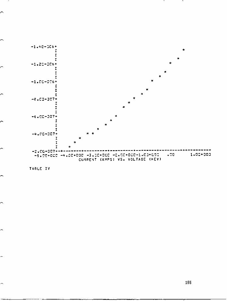
-1.4C-~C6+ r I I
-l.Z:-JCb+ r I I
-1.C'C-C::'6+ r I I
-8.CJ-JC7+ I I I
-6.CC-J07+ I I I
-4.PG-~C7+
I I r *
* >I<
>I<
*
*
>II *
-Z.CG-OC7+-*-------+---------+---------+--------+---------+---------+ -S.:C+Q~~ -4.~C+QaC -3.:C+OCC -~.Gc+acc-l.CJ+C~: .. ,., .--
CUQPE'lT (AMPS J VS. VOLTAGE (KEV'
TABLE IV
155

V JTOT JE JS;:C:: J6SCAT JI JS~CI .c:o -1.34-006 -2.9S-::b 8.14-:::7 =.19-~J7 6.65-CC8 1.0S-0C7
-Z.38-CCI -1 •. 27-0eb -2.72-C:6 7.76-JC7 ".9:-007 6.97-c:a 1.lJ-C07 -4.76-0£:1 -1.19-GC& -2.S9-aC& 7.4C-C:l1 4.1::-o:n 7.Z8-C08 1.l!:-C07 -1.14-::~H -1.12-:!~6 -2.47-CC6 1.G6-CC1 ".SC-O::n 7.6C-Q!:!8 1.21-:07 -9.52-~Cl -l.CS-OCb -Z.!6-C:6 6.73-CG7 ".29-001 7.9l-IJC8 1.27-007 -1.19+:JOC -9.78-001 -2.25-0::6 6.42-":07 4.09-J~1 8.23-JCa 1.33-:07 -1.43+COO -9.13-a~17 -2.14-a~6 6.l2-G(H 3.9:::-C:H 8.S4-JC!9 1.39-JG7 -1.67+0CO -8.51-CC7 -2.:14-0:6 5.a3-:~7 !.72-~iJ7 8.86-0£'a 1.46-JC7 -1.9C+Q~C -7.90-tJ~7 -1.~5-CD6 5.56-C07 3.55-t'rJ7 9.17-;)Ca 1.52-C07 -2.14+DOI: -7.32-CCl7 -1.36-G::!6 5.3C-C(!7 !.38-C:J7 9.49-:C5 1.59-Q07 -2.38+JOC -6.76-GC7 -1.77-G06 S.:J6-:;C7 ~.23-~a7 9.80-Q08 1.66-C07 -2.62+CCO -6.22-C07 -1.69-~iJ6 4.82-0:)7 3.08-CJ7 1.01-DC7 1.73-(;;07 -2.86+JCC -s. 7e-C~!7 -1.61-uJ6 4.6C-CJ7 2. Q 3-':C7 I.C4-C07 1.8J-:J07 -3. H'+JCC -5.2C-O:H -1.5!-C!J6 4.38-1):7 Z.8C-~~1 1.C7-0C7 1.87-C07 -3.33+:J00 -4.71-007 -1.46-006 4.18-C:)7 :.67-jJ7 1. 11-;)C7 1.94-~O7 -3.57+JC~ -~. 24 -::)7 -1.!9-C~~ 3.96-iJD7 2.54-:;:n 1.14-007 2.01-007 -3.81+JOC -3.79-CC7 -1.3!-GC6 '!.aC-CC7 2. 42-;~O7 1.17-0r7 2.:9-007 -".(,,5+:JC~ -3.3S-:H::7 -1.27-:;:b 3.62-CC7 2.31-:~7 1.ZC-JC7 2.17-C07 '"'"I, -4.:9+CC: -2.92-C!n -1.21-C:Jb 3.4S-C:l7 ~ .2'~-C~7 1.23-:lC7 2.24-:)C7 -4.S2+~CC -2.51-':C7 -1.15-:1)6 3.29-c:n 2.1:-0:17 1.26-UC7 2.32-:m7 -4.76+JOG -2.12-::1 -1.lJ-:06 3.1'+-:07 :.CO-CJ7 1.!':-;:)C7 2.~a-J07
q~SULT CURRENTS -4.1CC
CURRE~TS FOR POT~NTIAL OF -4.1J+G~~ KV
INCICENT ELECTQaN CURRE~T -1.:s-~a6
S~CONDA~Y ELECT~O~S 3.:9-C~7
~ACKSCATTERED ELECTRONS 2.29-C:7 I~CIDENT pqOTa~ CUQRENT :.21-C07
S~CO~DAoy ELECT~a~s 2.18-C~7
SULK ca~OUCTIVITY CURRE~T 3.23-CCQ
, CH~NGE ANGLE PREF e:.
PREFERED ~~GLE: 8~.rcc DESREES
PAPA~ET~RS
MATERIAL IS KAPT. EMISSION FOP"'ULATIO~ IS ANGL. VSACK : .co KEV VPHT = .ce KEV V3EGIN : ,.. ...
.... l.. KEV VEND : -s.uC+CC~ KEV ANISOTR::lPIC FLUX pQEFERED DIRECTION: 8:.~::J :JEGREES
156

~QATIO( 1) = 1.SQ+C~"
IRATIO( 1) = 1.~C+C~" ~~VIRON~ENT IS A SI~GLE ~AX~~LLIA~
ELECTRO~S: ~El = IONS NIl = TABLE ALL
1.!"a+a~6 ('1~*-!)
1. CG+a:l6 (M**-3) TEl = TIl -
5.:::CJ KEV s.cao KEV
157

T~BLE G~~E~ATED USING A~ISOT~O?IC INCIDENT FLUX AT B:.:C~+COC DEGR~ES
E~EQGY(KEV) EL. SEC. EL. BKSCAT. PP • SEC. • 1~C ~.s :3 .ZC5 .0'+1 .2r::C 3.698 .229 .:l66 .3JO 3.688 .289 • ~aa ."CD 3.4'+2 .333 .~93
.5!jO 3.18C .367 .117
.6~a 2.901 .392 .187 • n:1J 2.199 .41C .261 .8:10 2.525 .423 .336
1.QOO 2.128 .442 .'+86 2.C:J~ 1.256 .411 1.12C 3.0iJO .923 .381 1.6;jQ u.~OC .741 .353 1.987 s. Gi:C .625 .329 2.3l3 6.C::C .544 .3l: 2.591 1.C:C .U8 1l .295 2.850 8.COO .437 .28~ 3.078 9.CCC' .399 .273 3.285
lC.C:JC .368 .26S 3.476 2C.roC .216 .236 4.5C9 3C.COG .158 .232 5.313 40.C:C .127 .231 5.79'+ SC.CC: .1:7 .231 6.137
PLOT SEeD
158

,--
r
4.':'C+::C+ I :(l
« I
'" 3.CQ+CGC+
** r IlIr
I* I:(l
2.CQ+::ICC+ I I I
I '" r
1.CO+:~C+ :(l
r I ** r >Ir>lr*
I I *
.Ci: .or
*---------+---------+---------+--------+---------+---------+
PLOT 3~CK
1.CG+~Ol 2.C~+~Gl 3.uC+~Jl 4.C:+C~1 5.CG+QCl c.C~+~Ol
YI~LD (F~A::TIO"l) vs. ~N::RGY (KEV)
159

s.ce-eel+ I I I>;<
" .r:O-O(H+*
'" '" I >I<
*' :$
I '* 3. CC-J!Jl '"
I I
'* 2.CC-:Ol'"
I I I I
1.CC-:;~1+ I I I I
.ra *---------+---------+---------+--------+---------+---------+ .DC 1.~C+JCl 2.CJ+:Gl 3.c~+aJl 4.~O+OOl 5.C:+CCl 6.CJ+:Cl
YIELD (F~ACTICN) vs. ::""~RGY (KEV)
PLOT IO~
160
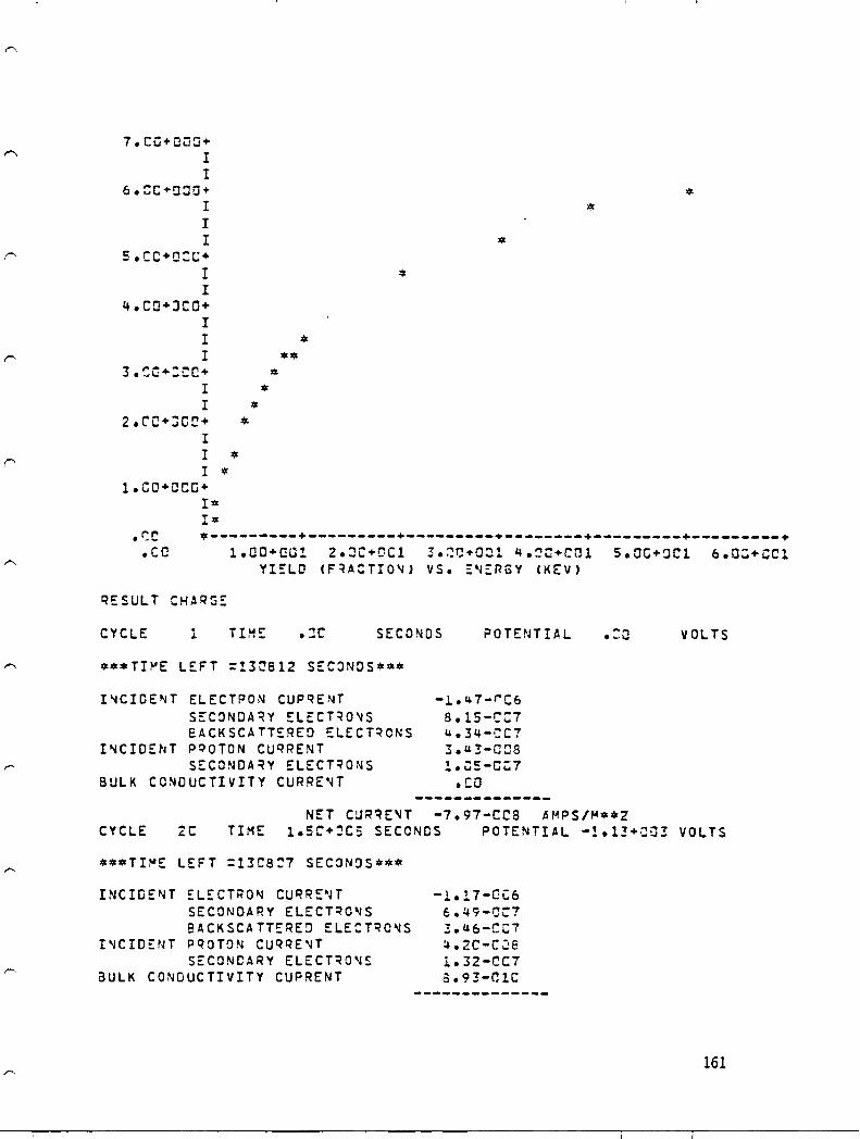
7.CG+OLiS+ I I
6.!:C+O::lO+ I I I
s.CC+O:t:+ I I
4.CO+JCO+ I
I * I *. I * I *
2.C'O+:C~+ * I I •
I * 1.CO+OCO+
I= I~
*
•
.~c *---------+---------+---------+--------+---------+---------+ .cc l.OO+OOl 2.~C+nCl 3.~O+OOl 4.~G+cnl 5.0C+~Cl b.a~+CCl
Yl~LO (F~ACTIO'lJ vs. ::'lERGY (KEv)
RESULT CHARSE
CYCLE 1 TIME .::r SECONDS PO TE~lT I A L
**.TI~E LEFT =!3~812 SEC~NOS***
I'lCIDE~T ELECTPON CUPqENT SEC~NDAqy EL~CT~O~S EACKSCATTERED ELECTqONS
I'lCIDE~T PQOTON CuqRENT SECONDA~Y ELECT~ONS
BULK CONDUCTIVITY CURRE~T
-.l..47- r C6 8.1S-C::7 4.34-':C7 3."3-088 1.C5-C:7
.CO --------------
NET CURqE~T -7.97-CCS AMPS/~**Z
VOLTS
CYCLE 2C TIME 1.SC+~CS SECONDS POTENTIAL -!.1!+~a3 VOLTS
***TI~E LEFT =13CS:7 SEC~N~S***
INCIDE~T ELECTRO'l CUQRE~T
SECONDARY ELECTqO'lS 8ACKSCATTERED ELE:TqO~S
I~CIOENT pQOTON CUQRE~T
SECONDARY ELECT~O~S aULK CONDUCTIVITY CUPRENT
-1.17-0C6 6.49-0C7 3.U6-CC7 ~.2C-C2E
1.32-CC7 a.93-CIC
161

TABLE CHARGE
***TI~E LEFT =130807 SECONJS***
***TIME LEFT =130SCZ SEC3NDS***
T (SEC) V (VOLTS) I(AMPS/I"**2) -------------------------------------------.co .DC -7.97-:C8
3.C6+0C3 -5.8'++~:JZ -3.aC-COa E:.IZ+C:3 -8.66+JJ2 -1.84-~~8 9.18+a~3 -1.0C+JJ3 -9.Cl-:C9 1.22+0C~ -1."'7+CJ3 -~.~1-~C9 1.53+0!:!4 -1.1~+G:!3 -2.17-L1t"9 1.84+004 -1.12+:~3 -1.Cb-C09 2.1~+ao~ -1.13+~J3 -5.23-:1: 2.45+0!:!4 -1.13+JC3 -2.57-:Hl 2.75+:04 -1.13+0;)3 -1.27-:1:
PLOT IV
162

,--
r
3.rO-~(!7+
I I I
I * I *
2.CJ-~07+
I I I I I
1.C!)-J07+ I I I I
... .., .1.. _
I + I I I I I
*
:$
*
:$
-1.CQ-:07+---------+---------+---------+--------+---------+---------+ .co
CU~RE'4T (AMPS) VS. VOLTAGE (I'EV)
R~SULT CURRENT -1.330
CURRENTS FOR POTE~TIAL OF -l.eZ+LC~ KV
I~CIDENT ELECTqON CUPqENT S~CONDARY EL~CT~O~S
6ACKSCATTE~ED EL::CTQC~S
I~CIOE~T P~OTO~ Cu~qE~T
S~CO~DARY ELECTRO~S
BULK CO~DUCTIVITY CURQE'4T
"lET CURRENT
LIST ENVI
~~VIRON~ENT IS A SINGLE "'AX .. ::LLIAN
ELECTRO~S: ~;E 1 = 1.C!:+a~6 ('1**-3) IONS . ~; I 1 = 1.:J+IJ:J6 ('1#:$-3) . CH~NGE ANGLE ::=;I4T .5
-1.':':-CC5 S.6S-CC7 3.:1-::::7 Q.b1-Ct.:8 !.::C-CC7 1.'+4-::9
4.f:3-CC8
TE 1 TIl
AI"PS/"1>il*2
= 5.U~C KEV - c: ,..,..,"", KEV - Jea.""",t.
1.0Q+:r:~
163

EQATIO= :.:~-CCl IRATIJ=
CHA~GE ANGLE IqAT .5
~qATIO= 5.~:-JOl IRATIJ=
TABLE ALL
164

TA6LE GENE~.a TED USING A ~J IS" T =l 0 PIC INCIOErJT FLUX AT a,:.ccc+':;QO OE:;R::ES
ENERGYP(EVJ EL. SEC. EL. EKSC.aT. Pp. SEC. r .1:0 2.573 .176 .:39
.21:0 3.zas .23: .:55
.:!:c 3.216 .269 .J67
.400 2.~:H .296 .:78
.5:0 2.661 .3:6 .1:98
.b~Cl 2.4::39 .!31 .156
.7:JC 2.236 .342 .218
.8~C 2.C40 'tc:" e_.."l. .281 1.CCC 1.742 .36! .4\..6 2.C:JO 1.~4E: .342 .936 3.C::lC .771 .324 1.337 4.cea .62C .!:7 1.661 ~ ,.. ... n _e_w_ .523 .294 1.934 6.C!:)O .455 .282 .2.171 7.r.O~ ."C4 .273 2.383 a.:oc .!65 .2b6 2.573 9.cac .334 .259 2.747
lC.COO .308 .25/,J 2.9(.6
r :z~.aQ~ .:'81 .::35 3.35! 3c.oor .132 .232 4.441 4r.C'GC .lC6 .232 ".843 -".. ..... -.., :: .• v..a .... .C89 .232 5.13:
PLOT SEeD
165

4.CQ+J!:C+ 1 I I >I<
>It
3.aC+~CQ* I >It
* I* 1*
2.0C+CCQ+* 1* 1* I I I
1.CO+QCC+ * I * I * I ** I .*** I
.co *-----~---+---------+---------+--------+---------+---------+ .00 1.GO+OCl 2.C:+CDl 3.CC+O:l 4.~:+~Ol 5.0Q+001 6.CC+aCl
YI~LD CF~ACTION) VS. E~~P'GY (KEV)
PLOT e~C~
166
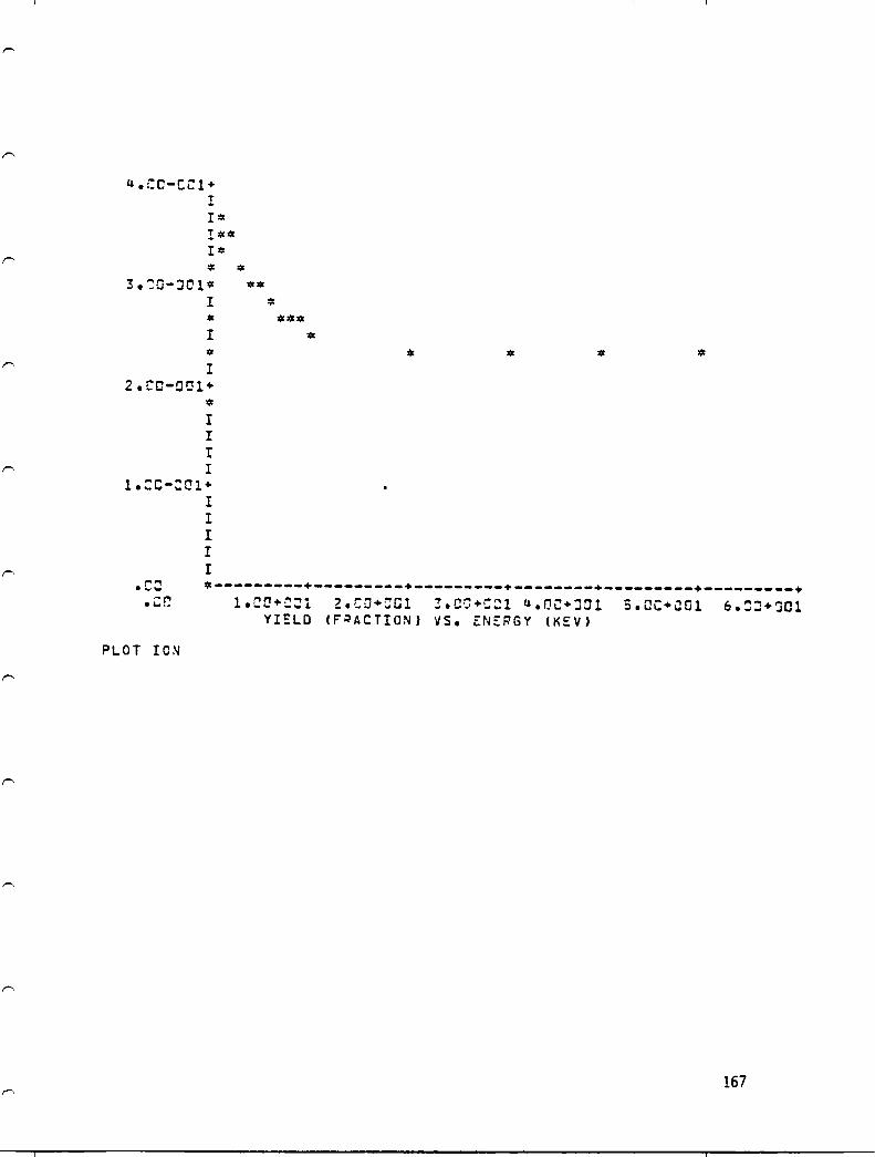
4.CO-CC1+ ! I* 1*11< I*
*' *' 3.~O-J"1'" "''''
I * • *'** I * '" I
2.CC-Ocrl+
* I I I I
1.::C-::Cl+ I I I I I
.c: *---------+---------+---------+--------+---______ + _________ + .GC 1.CO+C~1 2.CO+CGl Z.C~+C:l 4.0C+JOl S.CC+JOl 6.=J+~Ol
YIELD (F',;)ACTION) VS. EN~RGY (KEV)
PLOT ION
167

6.C~+J::!C'"
1 r r
5.C~+JCC+
I I I
4.CC+QCC+ I r I
!.CC+:OC+ * I '" I ** I *
2.CC+:JOC+ * I * I I "
1.~i:l+JCC+ >01
I
.c: *---------+---------+---------+-----___ + _________ + _________ + ... ,., ...... 1.:0+CC! 2.C~+~Ol 3.C~+C:! u.::+J'l S.CO+COl 6.0a+~Ol YIELD (F~ACTIO'J) vs. r:N::RGY O<EV)
RESULT CHA~G~
CYCLE 1 .JC SECONDS OOTE'HIAL :-f" . -- VOLTS
***TIME LEFT =13~796 SEC~NDS***
INCICE~T ELECTPON CUPRENT -1.76-0:6 SECO~DAqy ELECT~O~S e.14-C:7 eACKSCATT~RED ELECT~ONS u.78-C:7
INCICENT pOOTON Cu~qENT 4.1:-C:S SECONDARY ELECT~O~S 1.:S-UC7
SULK CO~DUCTIVITY CURRENT .co
NET CURqE~T -3.!a-CC7 4MPS/~**2 CYCLE 61 TIwE 3.76+JQ~ SECONDS POTE~TIAL -3.J3+CC3 VOLTS
***TIME LEFT =13a79Q SEC~NJS***
INCIDENT ELECTRO~ CUPRENT S~CONDA~Y EL~CT~O~S
BACKSCATTERED ELECTqO~S INCIDENT PROTON CUPqENT
S~CONDARY ELECT~O~S aUL~ CO~DUCTIVITY CURRE~T
168
-9.58-'1:7 4.44-C:7 2.61-C':7 b.57-CC8 1.d:-r.:':7 2.39-~:9
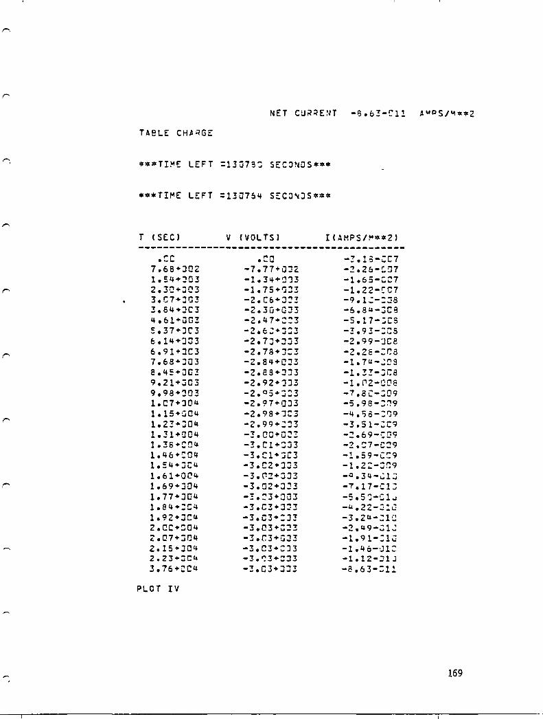
TA e LE CH" RGE
***TI~E LEFT =13078: SEC~NDS***
***TI~E LEFT =13u75~ SECO~JS***
T (SEC) V (VOLTS)
-------------------------------------------.r.c .~a -!.la-:C7
7.68+J02 -7.17+0:12 -:!.20-r.~1 1.S4+J03 -1.3'++~'J3 -1.65-~C7 2.3~+:;C3 -1.15+'jJ3 -1.22-:C7 3.C7+JG! -2.Cb+J~! -9.1':-:J8 3.84+::IC3 -2.30+0:l3 -6.84-:iC8 4.61+ij03 -2.47+::3 -S.17-:;Ca :.37+JC'3 -2.6:+J:3 -:!.93-:CS 6.14+:303 -2.7J+~J3 -2.99-:lC8 6.91+:JC3 -2.18+):3 -2.26-:r.8 7.68+:03 -2.8t;+C:l3 -1.7u-,;~S
8.45+JG! -2.8S+:l:!3 -1.3!-:JC8 9.21+~C3 -2.92+1:33 -1.i'2-~Cl8 9.98+~Q3 -2.o5+~:3 -7.aC-:Q9 1.C1+:JC\u -2.97+0J3 -5.98-::~9 1.15+004 -2.98+1::3 -4.158-:119 1.23+:)04 -2.99+::13 -3.51-:C9 1.31+004 -!.CO+O~~ -:.69-::09 1.38+~a4 -!.Cl+::B -2.:7-C::!9 1.46+:04 -3.:::1+'JC3 -!.59-C~9 1.:4+:JCu -3.C2+J::i3 -1.2:-J~9 1.01+QC4 -3.Cl2+JJ3 -O.34-~1:;
1.09+:::04 -3.0:?+:).:!! -7.11-C1] 1.17+J04 -!.~3+~u3 -5.S'J-S1.J 1.84+:JC4 -3.C3+J~3 -u.22-2!cJ 1.92+JC4 -3.C]+:::!! -3.2 11 -:1C 2.CC+:04 -3.C!3+CJ! -2.49-:1~ 2.01+J04 -3.C3+G:J3 -1.91-:1i:i 2.15+J04 -3.C3+:::!3 -1.46-~.1l: 2.23+:'C4 -3.~3+:::J3 -l.lZ-~l.J
3.76+CC4 -3.C3+:JJ3 -8.63-:a:.
PLOT IV
169

2.CC-C!:I7+ I
I '" I '"
1.r-C-:C7+ '" ! I I + I I I
-1.CG-Cr.7+ I I I
-2.r:':-C07+ r r I
-:!.OQ-OQ7+ I I
*
>10:
-4.~C-~C7+---------+---------+---------+--------+---------+---------+ -S.:C+CCC -4.CQ+QCC -3.::+~C: -2.CC+~OC-l.rC+~~c
CURRENT (AI"PS) VS. VOL TAGE (KEIJ)
TABLE IV
170
.ae 1.C:)+,JCO
-,
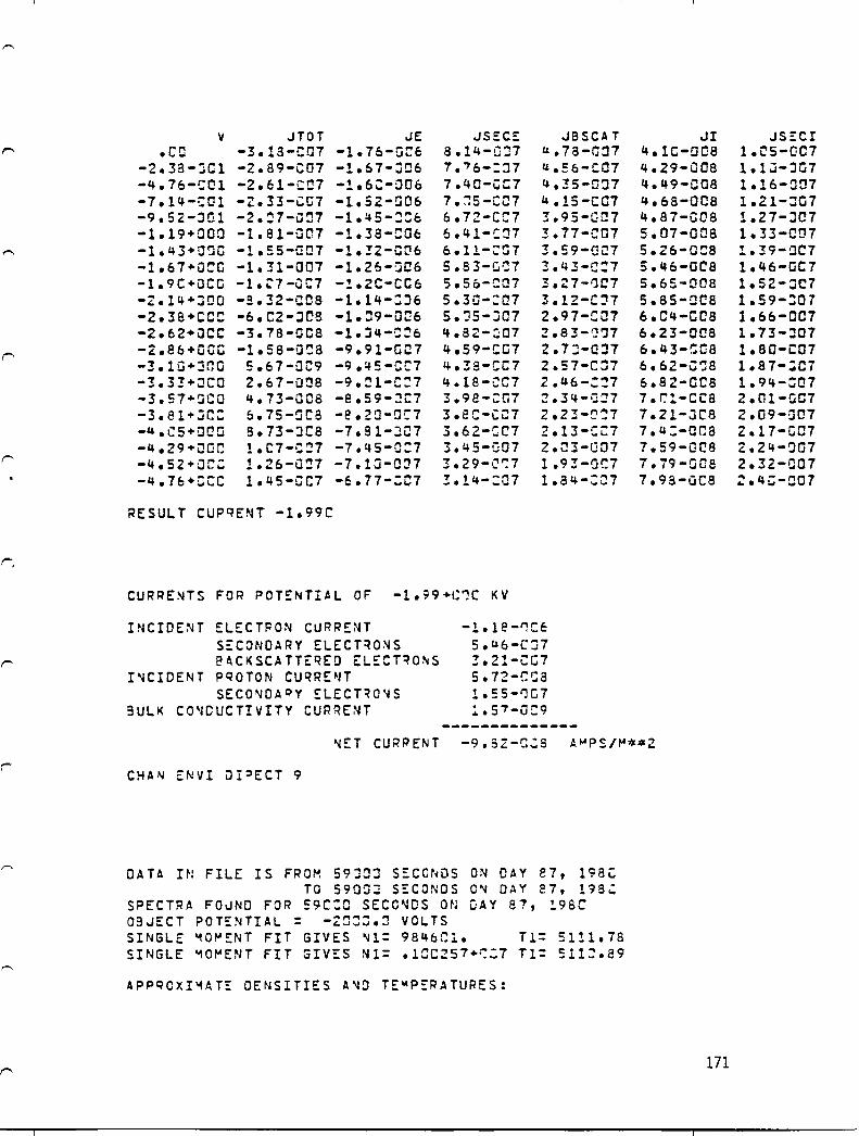
.,
V .JTOT JE JS~C~ JBSCAT .CO -3.13-C07 -1.76-G::::6 8.14-G::l7 u.78-0:17
-2.38-jC1 -2.89-C01 -1.O7-~O6 7.'76-::J7 u.~6-C07
-4.76-(;01 -2.E:1-CC1 -l.6e-D06 7.40-CC7 4.!5-G:J7 -7.14-::CH -2.33-CC7 -1.52-G06 7.~5-CC7 4.15-CC7 -9.52-301 -2.~7-U07 -1.45-::6 6.72-CC7 3.95-G~7
-1.19+000 -1.81-0C!7 -1.38-:06 6.41-~:J7 3.77-C(';7 -1.43+0'JG -1.55-001 -1.:!Z-C06 6.11-::'G1 3.S9-!JC1 -1.67+(jCG -1.31-001 -1.26-J06 5.83-G::7 !.43-C:1 -1.9C+OCC -1. ~7 -aC7 -!.2C-CC6 S.50-~a1 3.27-1)01 -Z.14+JOO -a.32-C08 -1.14-:::16 5.30-:07 3.12-c:n -2.38+CCC -6.C2-JOB -1.:l9-006 S.",S-:i07 2.97-G07 -2.62+0CC -3.18-008 -1.::;4-C~6 4.82-:::07 2.83-')"7 -2.86+000 -1.58-a~8 -9.91-GC7 4.59-CC7 2.7J-C:17 -3.1Q+Jeo S.67-0C9 -9.!f5-CC7 4.38-C07 2.57-C~7 -3.33+;:2CO 2.67-a~8 -9.~1-C:7 4.1B-CC7 2.46-::!1 -3.57+(:;00 4.73-008 -8.59-:11:7 3.98-:G7 2.34-Q~7
-3.81+~C: 6.75-(JC8 -e.20-D!:'7 3.eG-C~7 2.23-C~7 -4.C5+QCa S.73-:JC8 -7.81-:107 3.62-:C7 2.13-~i:i
-4.29+iJOC 1.C7-C~7 -7.45-0:7 3.45-007 2.~3-f.J07
-4.52+QC':: 1.26-0::n -7.10-0:n 3.29-C~7 1.93-1j!:7 -4.76+ijCC 1.45-CC7 -E.77-:C7 !.14-:a7 1.a4-:~n
RESULT CUP RENT -1.99C
CURRE~TS FOR POTENTI~L OF -1.99+C~C KV
INCIDENT ELECTPON CURRE~T
S~cONOARY ELECT~O~S e~CKSCATTERED ELECT~O~S
r~CIDENT PROTON CURRE~T SECO~DAoy ELECT~O~S
SULK CO~DUCTIVITY CURRENT
CHAN ENVI ~I~ECT 9
-1.1e.-'1Cc 5.46-C~7 !.21-CG7 5.72-CC3 1.SS-t'JC7 1.5 7 -0:::9
DATA IN FILE IS FROM 59JC~ SEca~DS ON DAY e7, 198C TO 59aa~ SECONDS C~ DAY E7, 196~
SPECTRA FO~ND FOR ~9C:C SECC~DS ON DAY S7, !9BC 03~ECT POTENTIAL = -4~::.J VOLTS SINGLE ~O~ENT FIT GIVES ~l= 984oCl. Tl= 5111.78 SINGLE ~O~ENT FIT GIVES Nl= .lCC2S7.~:1 T1= 511:.89
APpqOXI~AT~ DENSITIES A~D T~~P~RATURES:
JI Js::cr 4.1C-QC8 1.CS-QC7 4.29-008 1.1;J-:JCi7 4.49-0Q8 1.16-OtH 4.68-008 1.21-:07 4.87-008 1.27-J07 5.07-008 1.33-C!J7 5.Z6-0C8 1.39-QC7 5. 46-Ql~8 1.46-0C7 5.65-008 1.52-;JC7 5.8S-0C8 1.59-:07 6.C4-C08 1.66-007 6.23-008 1.73-:07 6.43-C08 1.80-C07 6.62-0':8 1.87-~C7 6.82-0C8 1.9~-:O7 7.r.:'-CC8 2.01-GC7 7.21-JC8 2.09-007 7.4:-cr.a 2.17-CC7 7.59-0CS 2.24-~O1 7.79-008 2.32-007 7.98-UC8 z.4C-C07
171

SCECIE 1 ( -1) 2 ( 1)
TABLE ALL
172
O::'.jSITY "'1-3) 9.85+"'05 1 • .)iJ+QC6
TEMP(E'l) 5.11+r::~! S.11+C:3

-,
,-..
TABLE GENE~ATED USING ANISOT~OPIC I~CIDENT FLUX AT 8:.~QC+cnc DEGREES
ENEQGY(I(EV)
.3=:iC
."CC
.5CO
.6J!:
.7JC
.8~~ 1.CQn 2.~OJ 3.:~~
4.0:!::1 s.re: 6.CGO 7.!:~C
S.C:l!: 9.CO: lC.~CC 2e.r'=:!': 3C.r.::c: 4:.1:01: 5C.C:!~
RESUl T CHARGE
EL. SEC. 2.573
3.215 2.937 2.661 2.4u9 2.236 2.C4C 1.742 1.046 .77! .62~
.52!
.455
.404
.365
.334
.308
.181
.132
.le6
.1:'89
EL. SKSCAT. • 17&
.,~,.. e,- __
.269
.296
.316
.331
.3"2
.3se
.363
.342
.324
.3.:7
.294
.282
.273
.266
.25 Q
.254
.~3S
.232
.232
.232
PP • SEC. .:39 .:;55 .~67
.378 • :98 .156 .218 .281 .4 J6 .936
1.337 1.6bl 1.934 2.171 2.3S! 2.573 2.747 2.91.6 3.853 ".441 4.31+3 5.13~
CYCLE 1 TI~E SECONDS POTENTIAL .QC
***TI~E LEFT =13J757 SECO~JS***
I~CIDE~T ELECTRO~ CUPRE~T S~CCNDARY ELECT~O~S 8ACKSCATTERED ELECT~ONS
INCIDENT P~OTON CURRENT SECO~OARY EL~CT~O~S
SUL~ CC~DUCTIVITY CURqE~T
-1.74-:Q6 8.29-C.J7 4.77-C~7
". J9-c.:a 1.:4-CC7
.:0
NET CUR~ENT -2.9a-~:7 A~PS/~**Z
VOLTS
CYCLE TI~E 4.21+~:4 SECONDS POTE~TIAL -2.82+:C3 VOLTS
***TI~E LEFT =130748 SECONDS***
INCIDENT ELECTRO~ CURRE~T SECONDARY ELECT~ONS BACKSCATTERED ELECTRONS
INCIDENT pqOTO~ CUqRE~T SECONDARY ~LECT~ONS
BULK CONDUCTIVITY CURqE~T
-9.96-\:'07 U..79-C~7
2.73-C;7 6.39-::'::;2 1.7B-uC7 Z.22-C't: Q
~ET CURRENT -8.89-Cll A~PS/~**2
TABLE CHARGE
173

***TIME LEFT =13a7~8 SECONDS~**
***TIME LEFT =13J74~ SECO~JS***
T (SEC) V (VOLTS)
-------------------------------------------.re .C:J -2.9G-::7 8.60+:102 -7.8:+~J2 -2.al-:J~7 1.72+(JC3 -1.33+~:n -1.u3-~a7 2.58+::J03 -1.73+003 -1.C!3-CC7 3.44+:103 -2.Gl+:lJ3 -7.52-JCS 4.30+QC3 -2.23+:~3 -5.5!-:08 S.16+!)Q3 -2.3S+CD3 -4.:6-0r.:8 6.G2+.J~3 -2.49+J::J! -3.CC-~Qa
6.88+0"3 -2.5s+a~3 -2.22-caa 7.7"'+J~3 -2.64+:)::13 -1.64-JCS 8.60+:C3 -2.69+~C3 -1.2Z-J::'.9 9.46+:JC!3 -2.72+)03 -9.t:t+-C:9 1.C3+::JC4 -2.75+CJ3 -6.71-CC'9 1.12+JG4 -2.77+J:3 -t&.98-.::9 1.2D+:1:4 -2.78+!:~3 -3.69-:("9 1.29+004 -2.79+:1!:3 -2.74-J('9 1.38+0(:4 -2.8lJ+JJ3 -2.~3-!):9 1.46+:04 -2.81+:JC3 -1.51-:;:'9 1.55+:104 -2.81+u!J3 -1.12-CrJ9 1.63+::4 -2.81+)'3 -8.31-::1 C 1.72+Q!:4 -Z.82+!:C!:! -6.17-::1: 1.81+:::!O4 -2.82+103 -4.58-:11 1.89+:1:4 -2.82+::13 -3.4 ;:-:::10 1.98+004 -2.82+:C3 -2.52-:1: 2.C6+!:H14 -2.82+J~3 -1.37-[1: 2.15+JC4 -2.82+:JJ3 -1.39-31":: 2.24+0~4 -Z.S2+!)::!3 -l.CE-':l":
PLOT IV
174

2.CQ-:JC7" I I * r * I '"
1.CC-::l7+
.co
I I I I + I I I
-1.00-007+ I I I I
-2.::C-OC7+ I I I I
*
* *
-3.CC-~C7.---------+---------·---------+--------+---------*---------+ 1.CQ+::!CJ -5.0C .. CC~ -~.uO+~~O -3.CQ+OUD -2.Cr.+OC~-1.~C+~ac CUqRE'H (A.r-'PS) VS. VOLTAGE (KC:V)
TA8LE IV
.co
175
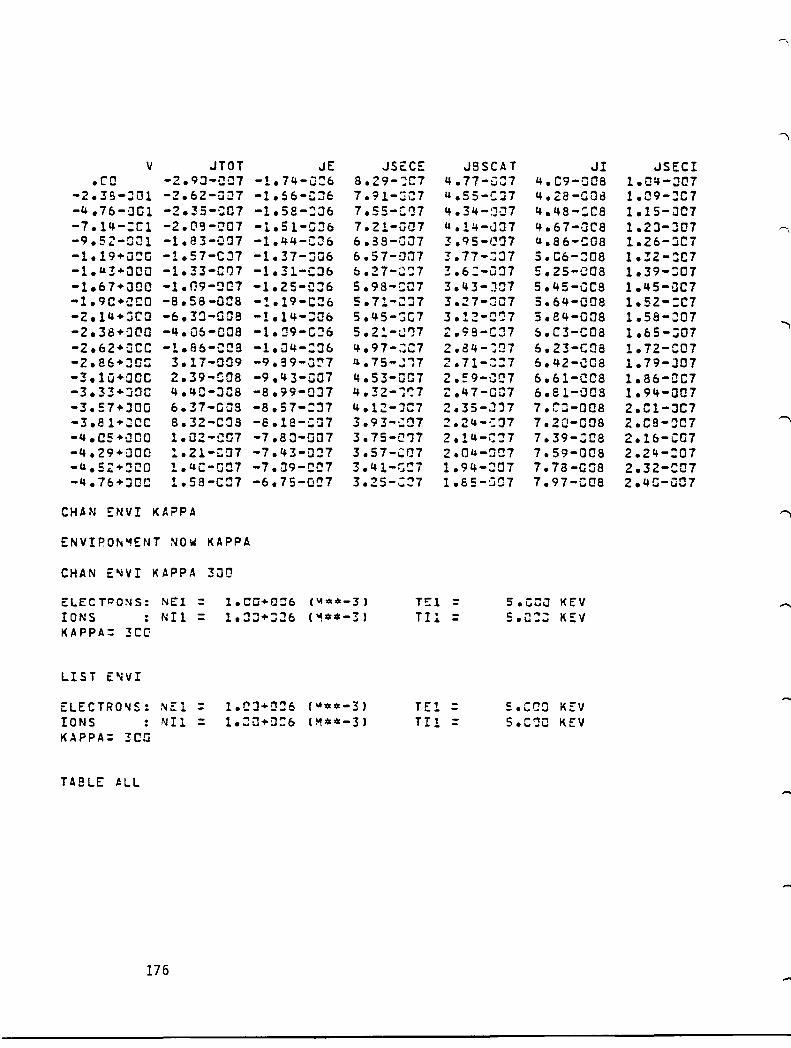
V JTOT JE JSC:C~ JSSCAT JI .ca -2.9J-~a1 -1.74-a:!6 8.29-~C1 4.11-C.:1 4.C9-C08
-2.3S-:lCll -2.62-Q:17 -1.56-C~6 7.91-:JC7 u .ss-c:n 4.28-COd -4.16-001 -2.35-~O1 -1.5B-:J6 7.SS-CIJ7 4.34-sa1 4.48-:C8 -7.14-:C1 -2.ClI3-~C7 -1.51-GJb 7.21-01:17 " .14-J:17 4.67-·jC8 -9.SZ-0~1 -1.83-Q~1 -1.44-COb 6.38-GJ1 3 .Q5-C~j7 u.86-C08 -1.19+u~0 -1.57-CJ1 -1.31-~a6 6.57-0:17 3.71-:'J1 S.C6-:ca -l. U!+OOO -1.33-C')1 -1.31-CJ6 b.Z7-~:7 !.6:-u:J7 :.25-008 -1.67+\)00 -1.r:9-~a1 -1.25-CJ6 S.98-C07 3.43-:101 S.45-CC8 -1.9C+CCO -8. S8 -aca -1.19-C06 5.7l-::n 3.::!1-:JC1 5.64-00a -2.14+::iCO -6. 3~-Qn8 -1.14-=00 5."S-:iC7 3.l2-~~1 5.84-008 -2.38+QI:'0 -".06-caa -1.:J9-CJ6 S.2!-~'17 '.98-C:J1 6.C3-C08 -2.62+QCC -1.86-cca -1.O4-:~6 4.97-:;C7 2.a4--:n7 6.23-C08 -2.e6+:JO: 3.17-009 -9.89-u::'1 4.75-Ji7 2.7l-':J7 &.42-CC8 -3.1(j+QCC 2.39-008 -9.43-C07 4.53-007 2.=9-tJC7 6.6l-CC8 -3.33+JOC 4.40-J08 -8.99-0:J1 4.32-"1r:7 ~.47-G!n 6.81-003 -3.57+JOO 6.37-GC8 -8.57-:::17 4.12-'):::7 2.35-';17 7.C:-008 -3.81+JCC 8.32-C~8 -S.la-ca7 3.93-::07 2.24-·:~7 7.20-C08 -4.05+uOO 1.02-C07 -7.80-Q07 3.7S-C')! 2.14-;:-:1 7.39-:C8 -4.29+UOC !.21-~a7 -7.'+3-Q:n 3.S7-C07 2.0u-~C7 7.59-008 -u.52+~~O 1.ue-G07 -7.09-CC7 3.'+1-GC7 1.94-~a7 7.78-C08 -4.1b+;JOC 1.58-ca7 -6.75-0C7 3.2S-:~7 l.8S-G!J7 7.97-C08
CHMJ ENVI KAPPA
ENVIPOr.t"lENT NO~ KAPPA
CHAN E~VI KAPPA
ELEC TQON s: NEI
IONS NIl KAPPA= 3eG
LIST E~VI
ELECTRO~S: NEl IONS "Ill K~PPA= 300
TABLE ALL
176
300
= 1.Cu+OC6 ('4""*-3)
= 1.::1:+:lJ6 ('1**-3)
= 1.CJ+Q:l6 ("·*-3) = 1.:::iJ+D:6 01·*-3 )
T::l = TIl =
TEl = TI 1 =
5.COJ s.c::
5.CC:J 5.C'JC
KEV K::V
KEV KEV
JSECI 1.Q~-J07
1.09-~C7
1.1S-JC7 1.2J-J07 ~,
1.26-:lC7 1.!2-:C7 1.39-~O7
1."S-QC7 1.S2-:C7 1.S8-~07 1.65-~O7 1.72-C07 1.79-307 1.Bb-OC7 1.94-007 2.C1-:JC7 2.C8-~C7
2.16-CC1 2.2'+-:07 2.32-CtJ7 2.4C-GC7

,-.
TABLE G~~E~ATED USING A~ISOT~OPIC INCIDE~T FLuX AT SG.:OC+COC DE~REES
ENERGY(KEV) EL. SEC. EL. BKSCAT. PRe SEC. .l:l~ 2.573 .~76 .::139 .2:C 3.3JS .23~ .:55 .!:lC 3.216 .269 .':67 .4DC 2.937 .296 .178 c:.,,., .-~'-- 2.661 .316 .~ge
.600 2."C9 .331 .156
.7a~ 2.436 .342 .Zla
.8~O 2.040 .3Se .281 1.C!:C 1.742 .3&3 .4;:6 2.C:lC 1.C46 .342 .936 3.CQO .771 .324 1.337 4.000 .62e .3J7 1.661 S.r'O~ .523 .294 1.934 6.C~C .455 .282 2.171 7.~:C .404 .273 2.3a! a.r::OQ .365 .266 2.573 9.CGC .334 .259 2.747
lC.C:;C .3ea .254 :.~C6
2C.!:JC .161 .235 3.353 3O.0JG .132 .232 4.441 ur::.c~c .1::16 .232 4.943 :o.oeo .089 .232 5.13:
QESULT CHARGE
CYCLE 1 TIME .JC SECONDS POTENTIAL .:0
***TIME LEFT =13~73S SEC~NDS***
I~CICE~T ELECTRON CUPqENT S~CO~DA~Y ELECT~O~S BACKSCATTERED ELECTqONS
I~CIDENT pqOTON CUqRENT SECO~DARY ELECT~O~S
SULK CO~OUCTIVITY CURRE~T
-1.75-':::6 8.UO-,:!:7 .. .dr-r.':7 4.C9-CS8 1.~U-[,::7
.':'J
~ET CUR~E~T -2.56-~C7 A~PS/~**2
VOLTS
CYCLE 56 TIME 4.18+~C4 SECONDS POTE~TIAL -2.8S+C03 VOLTS
***TI~E LEFT =13C727 SEC~NDS**~
INCIDENT ELECTRO~ CURRE~T SECONDARY ELECT~O~S 8ACKSCATT~RED EL~CT~ONS
INCIDENT PQOTON CU~RENT S~CONDARY ELECT~O~S
9UL~ CONDUCTIVITY CURRENT
TA8LE CHARSE
-9.93-CS7 4.76-':'J7 2.72-::C7 6.41-GC8 l.79-CC7 2.24-ryC Q
177

•• *TI~E LEFT =130727 SECONDS.**
***TI~E LEFT =13C719 SECJN~S***
T (SEC) V (VOLTS) I (A~PSII-'**2)
~------------------------------------------.ce .C:J -2.S6-:C7 8.54+\jC!2 -7.6g+~~2 -2.0C-:07 1.7:'+OC3 -1.32+0C3 -1.43-CI:7 2.~b+:JQ3 -1.71+:~3 -1.04-GC7 3.42+JC3 -2.QO+0;)3 -7.6o-:Ca 4.27+:lC3 -2.22+JJ3 -S.66-:CS 5.12+uC3 -2.33+::3 -4.Z!:.-C08 5.98+:03 -2.49+:1:3 -3.13-:C5 6.83+:C3 -z.Sa+;j~3 -2.34-:CE 1.69+CC3 -2.65+~:B -1.7S-:CS 8.s u +Gu3 -2.7;:)+3:3 -1.31-C!:8 9.39+;)03 -2.73+C~3 -9.84-:C9 1.r:'2+C:J4 -2.76+'JJ:: -7.39-:C9 1.11+:04 -2.7a+~~3 -5.5S-~C9
1.Z:+CG4 -2.8J+C03 -4.17-::9 1.28+::J4 -2.81+J:J3 -3.14-:C9 1.37+:C4 -2.82+~J3 -2.36-:CC; 1.4:+304 -2.83+:JC!3 -1.77-:'J9 1.54+:)[;4 -2.83+:1:3 -1.33-::9 !.6;::+:lO4 -Z.84+'.JJ3 -1.':~-:C9 1.71+C04 -2.84+D:'3 -7.55-·':lC 1.79+iJC4 -2.84+J:J3 -=.6a-;1~
1.88+~C4 -2.84+0:)3 -4.27-:1C 1.96+;j~4 -2.84+0J3 -3.21-':1: 2.05+:J04 -2.84+0:3 -2.42-':1':; 2.13+304 -2.84+Ja:: -1.82-:1~
2.22+3(,4 -2.8S+C:l3 -1.37-:1C Z.:!l+:J04 -2.85+::3 -1.r:3-:1S
PLOT IV
178 .....

,.......
-
2.CC-JC7+ I I * I * I *
1.CC-CQ7+ I I I I + I I I
-1.C:-OC7+ I I I I
-2.C:-Jr"'7+ I T ... I I
'" '"
'" '"
'"
-3.C~-CC7+---------+---------+---------+--------+---------+---------. 1.OQ+CC:J -5.CQ+DGa -q.:~+:O: -!.C=+JOC -:.~C+G:C-l.:~+JO: .GO CURRE'4T Ur-'PS) VS. VOLTAGE (KEV)
UBLE IV
179
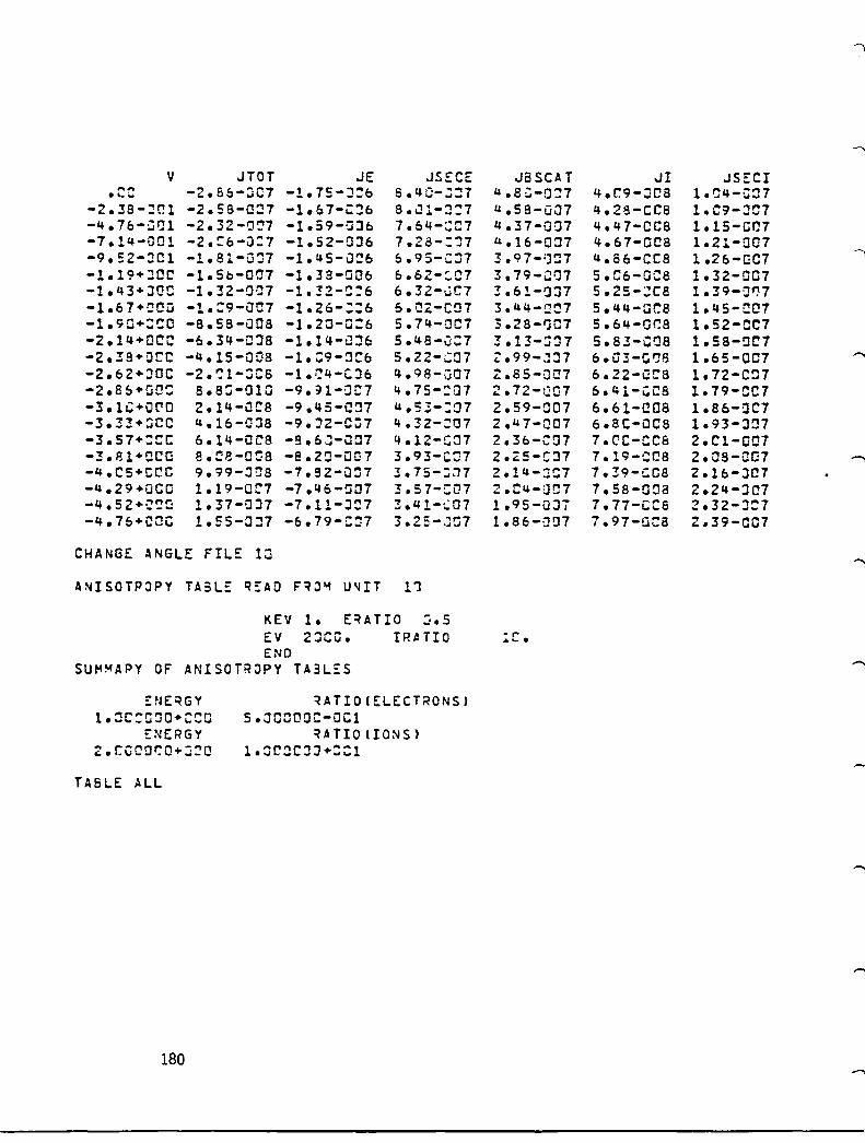
V JTOT JE JSECE JBSCAT JI JSECI .CC -2.86-:)07 -1.75-:1:b 8.40-;:H 4.8~-a:7 4.C9-;JCa 1. ~4-C:J7
-2.38-~('!1 -2.5S-0:J7 -1.&7-C~b S.Jl-:J:1 u .58-tJ~17 4.za-eea I.C9-JC7 -4.7b-~IJI -2.32-1J~7 -1.59-aJb 7.64-:';:1 4 .37-0~17 4.47-CC8 1.15-Gln -7.14-G!Jl -2.!:b-iJ:7 -1.52-036 7.28-:")7 4.16-037 4.67-0CS 1.21-007 -9.S2-:HH -1.8l-0:)7 -1.45-13:6 6.95-C::n 3.97-'):::7 u.S6-eca 1.26-GC7 -1.19+;)0(' -1.50-007 -1.33-0Q6 b.62-:07 3.19-aa7 5.eb-Dca 1.32-007 -1.43+JOO -1.32-Da7 -1.32-::6 b.3Z-l.iC7 3.61-0:)7 5.2S-:::C8 1.39-0117 -1.67+~CU -1. :9-ocn -1.26-::6 5. QZ-C~17 3.44-a~7 5.44-0C8 1.4S-C!J7 -1.9Q·:!:O -8.58-00B -1.20-0:6 5.74-007 3.28-1J07 5.64-Dr.a 1.52-CC7 -2.14+0CC -6.34-0::18 -1.14-:JJ6 5.48-u:':7 3.13-:J'J7 5.83-CtJ8 1.SS-!JC7 -2.38+!JCC -4.15-00S -1.:9-~Cb 5.22-C~17 Z.99-.1J7 b.G3-C'J8 1.65-0C7 ..... -2.62+:)OC -2.~1-~C8 -1.~4-C::l6 4.98-Ga7 Z.8S-0117 6.Z2-CC8 1.72-C!:n -2.8~+QO:: 8.8::;-010 -9.H-OC7 4.75-:07 2.12-:J07 6.41-CC8 1.79-0C7 -3.1C+QC'O 2.14-UC8 -9.45-C~7 4.53-:07 2.59-C07 6.61-COB 1.86-::JC7 -3.33+:JCC 4.10-0:18 -9.J2-C~7 4.32-:07 2."7-007 6.8C-QCS 1.93-J~7
-3.S7+:CC 6.14-0C8 -9.b.J-u07 4.12-C=:17 2.3b-C!:17 7.CC-CC8 2.Cl-Q07 -3.81+0CO 8.C8-008 -8. 2~-Q[:7 3.93-c:n 2.Z5-C:J7 7.19-CC8 2.08-007 -"""'\
-4.C5+CCC 9.99-JaS -7.32-Q~7 3.75-::17 2.14-JC7 7.39-[;08 2 el b-JC7 -4.29+000 1.19-0C7 -7.46-007 3.57-ern 2.c~-aC7 7.58-008 2.24-JC7 -4.S2+~~a 1.37-a:J7 -7.11-J~7 3.'1.1-:':07 1.95-0:)7 7.77-CC6 2.32-J:7 -4.76+COC 1.5S-::J::l7 -6.79-::7 3.25-.JC7 1.86-a~17 7.97-0~a 2.39-007
CHANGE ANGLE FILE 10
A~ISOTPJPY HaL:: q~AD Fq;Pi U~IT 11
KEV 1. E~ATIO ~.5
EV 2:JCij. IRA TIO .,. .......
END SUt'1~APY OF ANISOTRJPY TA3L::S
::NEQGY ~ATIO(ELECTRONS)
1.:JC:G~0+~CC 5.00000i:-OC1 ::NERGY ~ATIO(IONS)
2.CCCOr:'O+::i~O 1.:)C~C:JJ+::l
TABLE ALL
180

TABLE GENERATED USING ANISOTROPIC INCIDENT FLUX 4T 8:.Ca~+~cu DEGR~ES
ENERGY(KEVJ EL. SEC. EL. BKSCAT. PP • SEC. • 1GO 2.573 .176 .~4S
• ,:10 3.3:15 .23: .:&4 .!':!O 3.216 .2b9 .J711 .lIoa 2.93 7 .296 .:90
c::"'n ... _ .... 2.661 .316 .114 .6UC 2.409 .331 .182 .7:0 2.236 .342 .254 .3:0 2.C4Q .3S~ .3:!8
1.C:C 1.7~2 .303 .473 2.CJC' 1.C4!: .342 1.~91
!. C::H.' .771 .324 1.558 4.000 .620 .3:.7 !-.935 S.OOO .:2! .294 2.25! b.rao .455 .282 2.S3C 7.C~~ .404 .273 2.776 S.coo .365 .266 2.998 Q.CCC .!34 .259 !.2GO
1('. O~~ .Z;JS .254 3.386 2(1.C:;C .lS1 "7-.&. .... ::::2 4.489 3C.~:O .132 .232 5.17 4
40.C:::~ .1:;6 .232 5.643
5C.OOC .089 .232 5.977
RESULT CHARGE
CYCLE 1 Tr~E SECONDS POTPHHL ...... ._ ...
I~CIDENT ELECTPO~ CURqE~T SECONDAPY ELECT~ONS SACKSCATTEREJ ELECTqONS
I~CIDENT pqOTO~ CU~RE~T SECONDARY ELECTqONS
SULK CO~DUCTIVITY CURoE~T
-1.75-('i:6 e.4C-~C7
4.SC-CC 7
3.Sl-CCS l.:4-C~7 -., . -
~ET CUqRENT -2.~1-CG7 A~PS/~**2
VOLTS
CYCLE 58 TIM~ 4.1C+:C4 SECCNJS POTE~TIAL -2.95+C~3 VOLTS
***TI~E LEFT =13C7~7 SECONOS***
I~CIDENT ~L~CTPO~ CURqE~T SECONDARY ELECTqONS BACKSCATTEPED EL~CTqO~S
INCIO~NT P~OTON CUqRE~T SECONDARY EL~CTRONS
3UL~ CO~DUCTIVITY CUR~E~T
-9.73-r:C7 u.6&-r'~7
2.67-CG7 5.57-0ca 1.E2-C':7 2.!:-tJC9
~ET CURRE~T -9.3C-Cll AMPS/~**2
C HAN G E ~ ~~ V I TA N K 181

ENVIPON~E~T TYPE IS TANK. THE eEA~ £NERGY IS 2.r.+QCJK~V
THE BEA~ CURqENT IS 1.=-~~S AMPS/M**2 A~D THE GUN A~GLE IS 8J.~CD DEGPEES
CHANGE ~NVI pqEF O.
E~VIRON~ENT TYPE IS TAN~. THE BEAM ENE~GY IS 2.~+JO:KEV THE 8EA~ CURRENT IS 1.J-~C= A~PS/M**2
ANO THE GUN ANGLE IS .:OC O!GREES
ENVIRON~ENT TYPE IS THE BEA~ E~ERGY IS THE 5EA~ CURRE~T IS AND THE GUN ANGLE IS
CHANGE VEND -ZC.
TANK. 2.C+~OlKEV
1.~-JC= A~PS/~**2 .CCJ D~GREES
CHANGE ~~ISSION NOR~AL
E~ISSION FORMULATION IS ~O~~.
CHANGE ANGLE ALIGNED
FLUX ALIGNED
T~BLE ALL
182
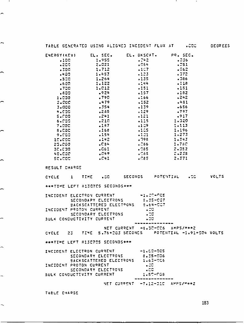
-
TA8lE GE~EqATEO USING ALIG'J::J INC!DENT FLUX AT .'::0::
E~ERGY(KEV) EL. SEC. EL. BKSCAT. pq • SEC. .loe 1.955 • :42 .J36 .21:0 2.021 .054 .::51 .:!ao 1.712 .1::7 .Co2 .'+00 1.45! .1:3 .:J72 .5:C 1.264 .135 .::l86 .600 1.122 .!.44 .118 .7:JC I.Cl2 .151 .151 .800 .924 .157 .182
l.COO .790 .!56 .242 z.coc .479 .152 .481 3.000 .354 .139 .656 4.CJ!:: .23S .129 .797 5.roo .241 .121 .917 6.(,,:0 .210 .ll5 1. :)20 7.COC .187 .1 ::9 1.113 B.CDC .168 .1:5 1.196 9.1:'0: .154 .L:1 1.273
lC'.cae .11.f2 .198 1.31.f3 2~.CuO .C84 •. ~86 1.7Se' 3r..CJO .C6l .~85 2.:J52 ItO.Cut' .C49 r'c: ... ~.- ~.238
Se'.!:Q!: .Clfl .;; a: 2.371
RESULT CHAqG~
CYCLE 1 TI1'lE .:0 SECONDS POTE'HIAL -,.. . ~ ..
I~CIDENT ELECTqO~ CUQRENT SECONDAPY EL~CT~ONS SACKSCATTEREQ ELE~ToONS
I~CIDE~T PQOTO~ CUqRE~T
SECONDARY ELECT~ONS 3UL~ CONDUCTIVITY CURRE~T
-l.:r::-r.C: 8.35-CG7 8.64-C:7 .:0
-I"' e_"': -... • ...JI.J
NET CURQENT -8.3C-~C6 ~MPS/~*~2
DEGR EES
VOLTS
CYCLE 23 TI~E 5.76+:03 SECONCS POTENTIAL -1.9l+C04 VOLTS
***TI~E LEFT =13C7~5 SECONDS**~
INCIDENT ELECTQON CUR~E~T
SECONDARY ELECTqO~S 3ACKSCATTERED ELECTqO~S
INCIDENT pqOTON CUqRENT SECONDAqy ELECT~O~S
3ULK CONDUCTIVITY CURRENT
U8LE CYARGE
-l.C:J-CCS 8.35-(Hi6 1.63-t:CC -... 'w" -,...
... u
1.5~-rQ8
183
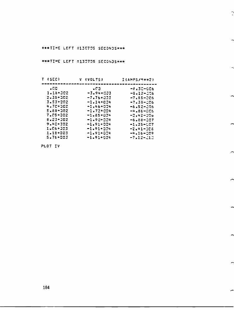
T (SEC) V (VOLTS)
-------------------------------------------.cc .rJ -8.3C-GCb 1.18+:02 -3.94+CQ3 -8.12-:':6 2.35+:102 -7.7b+~J3 -7.8S-::C6 3.53+:102 -1.14+C34 -7.38-:06 4.7C+JC2 -1.46+!JJ4 -6.52-.J06 5.88+)02 -1.72+C~4 -4.Sc-Ce6 7.(15+:)02 -1.S5+lJJ4 -2.42-:100 8.23+;)02 -1.9iJ+::!q -6.88-J07 9.4C+J!::!2 -1.91+!)C4 -1.35-C.07 1.06+J03 -1.91+~:!1+ -2. 4 1-JCa 1.18+0Q3 -1.91+0:4 -4. H:-:C9 5.76+003 -1.91+~(j4 -7.12-:1:
PLOT IV
184 -

-l.ce-oos+ I I I I
-8.~C-G::6+
r I I I
I I I
-4.C.'C-(J06+ ! r I r
-2.r:~-::C&+ I I I I
.:;0 lie lie >0: .;.
'"
>0:
.~o +-*-------+---------+---------+--------+---------+---------+ -2.C~+::1 -1.5C+:Ol -l.O:+~Cl -5.cc+~cn .a~ 5.0C+CCO 1.00+001
CURRE~T (AI'4PS) VS. VOLTAGE (KEV)
TABLE IV
185

V JTOT JE JSECE JBSCAT JI JS::CI • Or::: -3.30-C:::6 -l.~:-S~S 3.3S-CCH 8.64-::07 .CO .CJ
-9.52-CCl -B.26-C!!:!6 -1.~G-C~5 a.67-CC1 8.68-0:17 .CG .Co -1.9J+OCa -8.22 -Cr:6 -l.JO-:J::S 9.:'4-007 8.72-C:17 .CC .00 -2.8b+CGC -S.lS-Ge6 -1.:C-C:l5 9.~C-JC1 8.78-QC7 .CC .ao ---,
-3.81+:JCQ -e.13-CC'b -1.:0-~:lS 9.82-0G7 S.85-C~7 .au .co -4.1b+JC!C -3.C7-GC6 -l.JC-C:S 1.~3-CCb e.93-C~7 .C~ .~J -S.71+JOC -9.C:'-006 -1.:O-J05 1.~S-OC6 9. Cl3-:CJ7 .DC .OJ -b.67+~OC -7.qij-~C6 -1.JC-Cr15 1.14-:::6 Q .15-:::)7 .GO .co -7.62+:00 -7.86-iJCb -l.:J:-:OS 1.21-CC6 9.3C-C:J7 .co .O~ -8.S7+JCC -7.76 -C06 -1.J~-:05 l.la-ce6 9.147-~1J7 ....... .OJ -.-... -q.52+CC~ -7.65-C06 -1.):-::J5 1.37-iJC6 9.69-';07 .c~ .00 -1.C5+CCl -1.SZ-CC6 -l.::-C~S l."'-':!Jb c;.94-:J:J7 .CJ .C~
-1.14+301 -7.37-0:16 -!.::-:~s 1.6C-2!:!6 1.D3-G06 .C~ .co -1.24+CDl -7.1B-G06 -!.~r:-QuS 1.75-0C6 1.rb-C16 .cc .OJ -1.33+:)01 -6.94-C06 -!.JC-:lC5 1.9L1.-CC6 l.!l-::Jb .co .00 -1.43+:~1 -6.65-0C6 -l.~C-~CS 2.1S-iJC'6 1.16-COb .ca .co -1.52+~Ol -6.,6-006 -!.J~-O:J5 2.5:-~Co 1.23-C06 .co .O:J -1.62+CCll -s. 72-~~6 -1.'JC-:05 2.96-GCb !. :!l-Ga6 .DC .OQ -1.11+~Cl -4.90-C06 -1.~C-JC'l5 3.67-0C6 1.41-~u6 .r: .!JJ -1.61+:::a -3.5C-QCb -1.:0-:)05 4.96-u~b 1.!:3-C:b .ce .oc -1.9C.+COl -1.59-0C7 -l.~C-C:S 8.18-:~b 1.64-r::~6 • ~u .C:l
EXIT
C::XITJ
186
6. NASCAP*TERMTALK
TERMTALK has been revised to display SINGLE cell information in the same manner as NASCAP. The new SINGLE keyword, I SUMMAR I , causes TERMTALK to give the user a breakdown of the incident currents for a particular surface cell. To make this possible NASCAP has been modified to write this new information on file 21. Using NASCAP data files that have been generated from older versions will lead to a warning, stating that the I SUMMAR I option in the SINGLE module may not be used. The SINGLE module will, however, handle all other cell information as before.
The new TERMTALK output, in the single mode, is shown below.
187

~ CHOOSE A~Y MODUL~ HELP IS AL_AYS AVAILABLE - TYPE 'HELP'
)SINGLE o SINGLE COMMAND OR ~OOE SET ?
>EVERY HODE RESET
o SINGLE COMMAND Oq MODE SET ? )2
-~---------------------------------------------------------------------J SURFACE CELL NO. Z CODE 3104CS166C4! CENTEpEa AT -S.C -3.5 -2.5 ~ATERIAL IS _HIT NORMAL -1 0 J SHAPE IS SCUAPE
POTENTIAL =-1.37S+r;03 VOLTS I~TERNAL FIELD ST~ESS =-2.118+~02 VOLTS/METE~ EXTEqNAL ELECTPIC FIELD =-1.323+QC3 VOLTS/~ETE~ DELTA V =-1.~SQ-r.C2 VOLTS UNJE~LYI~G CONDUCTOR IS NU~9ER 1 UNOE~LYING CONOUCTOP POTENTIAL =-1.375+003 VOLTS A~GLE _ITH ANISOTROPIC DIRECTION 4S.QC3 DESS
FLUXES IN A/M**2 INCIDE~T ELECT~ONS
qESU~TING S~CONDARIES
~ESULTrNG BACKSCATTER INCIDENT PROTO~S
RESULTING SECO~DA~rES BULK CONDUCTIVITY PHOTOCUPRENT
NET F~UX AFTER ~O~G-TI~E-STEP a SINGLE CO~MAND Oq MODE SET ?
>EXIT
1.98-C:6 4.a7-C~7
Ll.92-CC7 4.43-IJOa ~.32-G:J3
-1.25-C 11 .CC
-7.57-C07
Ne\'i TERMTALK
188

7. NASCAP/LEO
7.1 GENERAL
The BIGLEO and BIGFINE codes are designed to study the electrostatic potential and sheath structure in the vicinity of a large, high-voltage spacecraft, and consequent current collection by the spacecraft, given specified fixed spacecraft potentials with respect to the surrounding plasma. BIGLEO performs the calculation for a large spacecraft, and has mirror plane capability. BIGFINE performs the calculation for the region above a periodic surface (e.g., a solar array module) and takes potential and current boundary conditions from the BIGLEO code.
BIGLEO and BIGFINE are written in FORTRAN V for UNIVAC 1100 series computers. They share many routines in common (BIGFINE has only twelve (12) unique subroutines) and utilize numerous NASCAP routines. Object definition, options, and control statements retain great similarity to NASCAP. Current trajectory plots are generated directly by BIGLEO and BIGFINE with some degree of flexibility. Object plots may be generated by OBJCHECK or NASCAP, and potential contours by POTPLT. Both codes write restart information on files 15 and 21. Additionally, file 16 contains information passed from BIGLEO to BIGFINE.
7.2 MAIN CODE MODULES
The major code modules in the BIGLEO and BIGFINE codes are
RDOPT [lun] OBJDEF [lun] POTENT [lun] CURRENt [lun] MOVEP [lun] APRT [n name] END
189

As with NASCAP, RDOPT must be executed first in any run. Repeat calls to RDOPT will (unlike in NASCAP) begin by resetting options to their initial values. The OBJDEF module requires input similar to NASCAP's OBJDEF. POTENT solves a nonlinear Poisson's equation, and CURRENt calculates the current to various parts of the object and generates plots if requested. APRT is used to print the potential array, and MOVEP moves the potential array from file 15 to another file.
7.3 RDOPT MODULE
The RDOPT module reads the run options from file lun (default 5, i.e., runstream). Available options for these codes are:
END End of input.
NZ nz Z-dimension of mesh; default = 17.
NG ng Number of nested grids; default = 1.
XMESH x
ERRLIM v
PDAMP f
ITERMX m
COARSCale
PCOND icon
DEBYE LENGTH d
SATVEL vx vy vz
BIAS icon v
190
Physical mesh spacing (m); default = 1.
Error parameter for potent (q.v.); default = 0.5 volts.
For each major potential iteration, mix f of previous iterate with (I-f) of current iterate; default: f = O.
Maximum number of major potential iterations; default: m = 100.
(Fine code only.) Resolve screening length to value appropriate to coarse code (16 x XMESH); default: resolve to XMESH.
Specify potential of conductor icon in volts; default: v = 1000*icon.
Ambient plasma Debye length em); default: 1 m.
Spacecraft velocity em/sec); default:
Bias conductor icon v volts relative to conductor 1 (see PCOND).
O. -

-
IONMAS mass [AMU]
TEf4PER t
PLOT UNIT [1 un]
PRINT CURRNT J PRINT TRAJEC PRINT SHEATH PRINT OBJDEF NOPRINT OBJDEF
SHEATH BOUNDARY v
LIMIT PLOTS xmin,
NSTP n
LUNPQV 1un
MIRROR plane
FINE CELL icell
FINE MESH xmesh
IZBOT i
Ion mass in kg or amy· default: 1.67 x 10-z1 kg.
Plasma temperature (eV); default: 1 eV.
Perform plots using unit 1un as a scratch file. Default is no plots. If lun is omitted, it is set to 28. If lun < 0, plots are made from previously saved file 11unl.
Options for diagnostic print.
Potential at sheath boundary to be used by CURRENt module of BIGLEO code; default = 100 V.
xmax, ymin, ymax, zmin, zmax Plotting limits in grid units. For trajectories projected on the Y-Z plane, only segments between xmin and xmax are plotted, etc.; default: plot full trajectories.
Maximum steps per trajectory; default: 100.
Unit number of fill to be used to write (read) fine cell particle information; default: 16.
Pl ane = I +X I, I -X I, I +Y I, 1_ Y I, I +Z I, I -Z I •
Establish mirror plane on specified boundary of inner grid.
(BIGLEO) Output information for cell icell for use by BIGFINE. Maximum of ten (10) cells.
(BIGFINE) Retrieve information appropriate to cell icel1 from previous BIGLEO run.
(BIGLEO only.) Resolution of previously specified fine cell; default = XMESH/16.
(BIGFINE only.) z-val ue for "bottom" of space, i.e., height of cell = NZ-IZBOT. Used in calculating VTOP.
191
NEMITX n (BIGFINE only.) Allows coarsening for current emission, i.e., number of mesh units apart for particle emission points. Number of particle emission points
NX-1 NY-1 = NEMITX x NEMITY
NEMITY n
VECODE v
default: NEMITX = NEMITY = 1.
(BIGFINE only.) Code velocity of emitted particles at surface; default: 0.1.
7.4 OBJDEF MODULE
The OBJDEF module is invoked by the specification OBJDEF lun, where lun (default = 5) is the logical unit number of the OBJDEF input. The input differs from standard NASCAP input in the following ways:
192
1. The only allowed building blocks are RECTAN, PLATE, PATCHR, and PATCHW.
2. All materials are assumed conducting. 3. For the BIGLEO code, surfaces lying in a mirror plane
should remain undefined. This will result in numerous warnings. It should be verified that the warnings refer to points in the mirror plane.
4. Similarly, for the BIGFINE code surfaces on the x- and y-boundary planes should remain undefined. There should be no surfaces on the z-boundary planes.

7.5 POTENT MODULE
The POTENT module solves the equation
where p, the charge density, is a function of the local potential, density, and temperature. The function used,
D = max(AD' O.7l)
reduces to Debye screening (within the code resolution, l) for low potentials, and to the density associated with the one-sided plasma thermal current at high potentials. At present, the input only allows for a constant ambient density and temperature. However, it is easy to modify the code to use an analytic formula for density and temperature as a function of position. The boundary conditions, for the BIGlEO code, are zero potential at boundaries and zero normal field at mirror planes. For the BIGFINE code, periodic boundaries are used in the x- and y-directions. User-specified potentials (which should average to the potential, VBOT, for that cell in the BIGLEO code) are used at the lower z-boundary, and at the upper boundary
VTOP = VBOT + (NZ-IZBOT)*XMESH*EZ where EZ is the normal field taken from the BIGLEO code. (It should be noted that the BIGFINE code, with its small mesh spacing, can provide far more screening than the BIGLEO code, so that the user may
193

need to specify a small value of NZ. As a rule, NZ should not be much greater than the scale of potential variation at the cell bottom.}
POTENT solves the nonlinear equation £0726 + p(6} = a by successive linearizations about the previous iterate. The scheme goes as follows:
1. Given iterate 6(n}, write
2.
194
-~ n+ 1) (6 ~ n+l) ) = 6 ~ n+ 1} d p i
P1 1 1 aii 6~n}
1
(n) dPi - 6. -::T"
1 dJl.: 1 (n)
6. 1
Using the finite element formulation and scaled conjugate gradient equation solver, minimize (to solve for 6(n+1)}
iff ~~(n+ll 2 + 1 dP 6(n+1)2 2'air (n)
6. 1
Require two orders of magnitude convergence.
3. Calculate the root-mean-square change
r ~ (~\n) _ ~\n+l) ) 2 E = ---'~--------------
1/2
2: 1
i
If E ~ERRLIM, finish. If E > ERRLIM, return to (1).
This scheme usually converges in 3-10 major iterations.
7.6 CURRENt MODULE
The CURRENt module calculates the current incident upon, and power loss by, each conducting segment of the test object. In the BIGLEO code this module operates as follows:
1. Define the sheath boundary as I~I = ~B' where ~B is the sheath boundary potential.
2. Determine the electron (for ~ > 0) or ion (for ~ < 0) current through each sheath segment, taking account of thermal and primitive ram effects. (See below.)
3. Track appropriate particles inward from each sheath segment. 4. Summarize results; make particle plots as requested.
In the BIGFINE code, the particles which hit the surface cell in the coarse code are duplicated
NX-l NY-l NEMITX x NEMrTY
times and emitted above the finely resolved surface.
195

7.7 MOVEP MODULE
The MOVEP module writes the potentials on logical unit lun (default = 10). The intent is to enable use of POTPLT to generate potential contour plots.
7.8 APRT MODULE
APRT prints the values for n gridsworth of array 'name'. The default is to print the potential for one grid.
7.9 INTERFACING THE BIGLEO AND BIGFINE CODES
If the BIGFINE code is to be used on selected surface cells, those cells should be identified by number in the options file of the BIGLEO code. Up to ten cells may be specified. Potential information for these cells will be written on file 21, and particle information on file LUNPQV [16]. Before invoking the BIGFINE code, files 16 and 21 should be copied over. The mean surface potential of the module specified in the fine code object definition and options should equal the potential of that cell in the coarse code. The potential and particle information will be retrieved upon specification of the coarse code cell number.
196

r'
7.10 TREATMENT OF RAM EFFECTS IN BIGLEO CODE
The BIGLEO code only includes an estimate of ram effects on sheath boundary currents. Ram effects are not included in sheath or shielded region densities. Thus this treatment is extremely primitive and should be employed only with great care.
Notation:
-3 p plasma density (m ) 9 plasma temperature (eV)
1s spacecraft velocity (relative to plasma) E electric field A
E electric field direction A
n outward normal to sheath vth thermal velocity m particle mass (kg) J current density (A/m2) in spacecraft reference
-+-distribution function (sec3 m-6) fey)
jth one-sided thermal current ~ sheath boundary potential q particle electric charge
-+-v particle velocity
A fundamental quantity in the LEO code is the one-sided current of an attracted particle species through the sheath surface. This is given by
-+- A A f -+- -+- d3; J·n = n • ev f(v) n
-+- -+- A
where v e: n iff v·n < o. Now
-+- -+- -1/2 -+- -+- 2 - ~2]/e9 fey) = fo(v) e m[v + V )
S
197

It follows that
where
-00
00
f -i/2 = -jth (z+Z) e dz
-Z
Z = V on(m/ee)1/2 s
_00
:jon = 12 - exp(-z2/2) + Z(~/2)1/2 (1 + erf(Z/~») Z < 0
Jth exp(-Z2/2) + Z(~/2)1/2 (1 - erf(-Z/IZ») Z < 0
12 A + = ,:!:7500 or 0, these formulae give the following For n = 10 ,noVs values for Ijo~l:
A + H+ 0+ e noV e s
0.1 -7500 7.9 x 10⁻³ 1.8 x 10 -6 2.0 x 10⁻²⁵
0.1 0 8.5 x 10⁻³ 2.0 x 10 -4 4.9 x 10 -5
0.1 7500 9.1 x 10⁻³ 1.6 x 10 -3 1.3 x 10 -3
1.0 -7500 2.62 x 10 -2 2.0 x 10 -4 1.5 x 10 -7
1.0 0 2.68 x 10 -2 6.3 x 10 -4 1.6 x 10 -4
1.0 +7500 2.74 x 10 -2 1. 7 x 10 -3 1.5 x 10 -3
The above values are calculated from subroutine DISMAX (DISplaced MAXwellian), and are used by subroutine FLUX to return current density and initial velocity of the sheath particle as follows:
198

Provisionally:
,-.
~ = -v + [2e(e + 1~1)/m]1/2 S E . s e
If
then
; = vth ~ E •
r
199

7.11
200
SAMPLE RUN OF BIGLEO AND BIGFINE CODES
if:L T ,1.S ELT SQ1-SlC
1 • .. . -3 • ... S. ". 7. a. 9.
1:'. 11. 12. 1l. 1 ... IS. lb. 17. la. !~: H. ZZ. 2.3.
~~: Zb. ~7. zs. 29. J :a.. !l. 3Z. 33. !'+. 35. 3b. !7. !d.. 39. ", .. "1. "2. "3 • ..... "5. "". "7. IIa.
.. SEPSOPT ..
Runstream for sample run.
~LT .. S~PSCPT ..
iELT,LS ELT ~RI-S!C
1.
iHOI>
Z. 3 • ... 5.
- O. 7. ~ . 9.
Ie. 11. 1Z. 1.3. 1 It.-1:. le. 17. 1S_ 19. 2e. 71. ~2. 2.3.
Options input for coarse code sample run.

!:L.T
~ELT,I.S ~I.T 3Rl-S3C
1.
i,;OG
i! .-3. 't. S. I>r 7. a. 9.
lii-_ 11. lZ. U. 1,+_ 15. lb. 17. 1~_ 19. ZOe
• I.EOT':ST •
Options input for fine code sample run.
L~O HIGH-VOLTAGE CURRE~T CCLLECTIC~ CODE
•••••••••• R'OPT 5 FINE CELl. 3:;: F'IN!: CELl. 4~0 NOPI1INT OIlJOEF NZ 33 MIRROR -Z ~C Z ERRLl" .1 PCO"O 1 -193. BIAS 2 !:I. SUS ! lC~.
a lAS 4 Z::J!l. BIAS 5 :!. alAS 6 100. BIAS 7 IS::;. x"ESH .3 PLOT u .. n Z~ lIMIT ;>LOTS ;. 10. OESYE LCI;(;TI1 .:::03 TCI1PEl?lTUllE .1 S~EATH 90UNOARY 1. ION "ASS 16 AI'U SATVCL o. 751:0. ~.
Eo,O LIMBOI: 3.CC-!l3 '1 PLIS"A OC'.SITY :
PCONOI 71 : -1.9a+OZ VOL TS. PCOf,jOI !I : -q.·0+01 VOL TS. pco'or 41 : ~.~o·o: VOLTS. PCONOI 51 : -1.9a+oz VOLTS. PCO'.o r 61 : -<;.80+01 VOLTS. PCO'jOI ." : -4.aO+Ci1 VOLTS.
'Y. ' ~ . _. 17. 18.
T: 1.CO-01 !:v SIoElTH BOU·jOAR"': 1..14+11 11 •• I-J) I~" "'55: :.bS-Zb KG.
SATELLITE J!:LCCITY:I ~.':C 7.:C-C! :.::10 I "'SEC.
Z FI'jE CELLISI CHO!E~: 1 CELl. NC. lee Z CELl. NO. ..CO
•••••••••• oRwOEr s
.01se "ETER ~ESCLUTICN
.0188 ~ETER I1ESOlUTICN
I.Ole-CO EV
Coarse code output - option specifications.
201

)
N o N
)
.SGfIL: rILE 17
OffSET 0 0 :l
CONtUCTOR 1
RECTAN OBJECT NO. DEfIh£D.
SLRFACE .x 'iOLJ SLRfACE -x 50LD SURf"ACE .y GOLD SLRflCE -Y 'iOLD SURfACE .Z GOLD ENDOBJ
RECTAN O~JECT NO~ OEfI~ED.
SLRFACE .x r;OLD Sl;RFACE -x 'iCLD Sl;R FACE .y '>OLD SLRf'AC[ -Y COLD SURfACE .Z GOLD ENDOBJ
PLATE THIN PLATE he. DEFINEO.
TOP -11 GJLO SOTTO" .X GOlC ENDOBJ
PLATE THIN PLATE NO. DEFINED.
TOP .2 GOLD ENDOBJ
RECTAN
)
ISTAT: DaCC~~DnGOOO
9<X< 12 7(y( II 1<Z( 3
1:?(~( 16 ~( Y( 10 1< Z< 2
IQO( Iq 6< Y< 12 I<Z< q
9<X< 12 6<Y< 12 1< Z< I
BIGLEO object definition output.
) ) )
OBJECT NO. DEfI~ED.
1!:<x< 11 5<Y( 13 q<z< 5
SURFACE .X GOLD SLRFACE -x GCLD SURFACE .y 'iOLD SLRFACE .z r;OLD SURFACE -Y GOLD SURFACE -2 GOLD ENDOBJ
PLATE THIN PLATE ~O. DEfINED.
Hx( q
7<Y< 11 1<Z( q
TOP +X GOLD BOTTO" -x GOLD ENDOBJ
CONDUCT OR '1
PLATE THIN PL~T[ ~O. DEfINED.
l1<X< 11 50( 1! q( ~( 13
BOTTO" -l( GOLD (NDOBJ
CONDUCT OR
PLATE: THIN PLATE NO. OEfINED.
110< 11 ~<Y< 13
1!<Z< 2!
BOTToM -x :iDLD ENDOBJ
CONDUCTOR q
PLATE THIN PLATE hO. CEfINED.
II(X< 11 5(y( U
Z!<Z< 3]
BOTTOM -x GOLD
) ) ) ) -)

N o w
) ) ) )
ENoOBJ
CONDUCTOR 5
PLAT[ THIN PLAT[ ~OW ~~fIkED.
TOP .X GOLD [NoOBJ
CONDUCTOR 10
PUTE
110( 11 5<Y( 13 q(z< 13
THIN PLATE kO~ oEfI~(D.
TOP .X GOLD EkDOBJ
CONDUCTOR 7
PLATE
110( 11 50( 13
13<Z( 23
THIN PLATE NOW DEfINED.
lOP .X GOLD ENoOBJ
[NOSAl
110( 11 S<Y( 13
ZHZ( 33
550 VOLU~E CfLLS NUMPEqEC BY ~U~LTB.
CALLl~G GEN-TL .AR~lNG secyc [qRCR I~ ANALYSIS OF SUOFAtE ~ROU~D V~RTEX 11CbOI
COCE: .ARNl~G secyc E~ROR IN A~ALYSIS OF SUPFICE AROUND VERTEX 11C701
COCE: 2 .AR~lNG secyc EPROR I~ J~ALYSIS OF SURFACE AROUND VERTEX 111C01
corE: Z dRr.ING
CODE: ;: IUR,,"ING -
CODE: Z .ARIlING -
COCE: 2 .ARNING
COCE: .. ARr.I"G
sccYC EDRCR I~ ANALYSIS CF SURFACE AROU~o vERTEX 111101
secyc ERROR l~ ANALYSIS OF SU~f'CE AROUND VERTEX 111201
secye ERROR 1'1 ANALYSIS OF SURfACE AROU~D VERTEX 111301
secyc LRROR l~ AkALYSIS OF SURfACE AROUND VERTEX 111qOl
SCCYC ERReR 1, ANALYSTS Of SURFACE AROU~D VERTEX llebOl
COCE: 2 .ARNING -
COCE: 2 .ARr.I~G -
COtE: 2 .AR"ING -
COOL: 2 .AR"I"C
CODE: .AR"ING
COCE: 2 wARNI"G
co CE: 2 WARt-INC
CODE: 2 "AliI-.INC -
CODE: 2 .ARNI"G
CODE: .ARIIINC
co CE: 2 .AR"It;G
CODE: 2 .AR"INC -
CODE: ;: .AR"IrjC -
eOCE: 2 .ARt-INC -
eOCl: 2 .AR t, I NG -
eoc£: ;: wAR'-ING -
COCE: 2 .ARNINC -
COCE: 2 .AR"It.G -
CO [[: 2
)
INSLST --
) ) )
secye EDROR 1" ANALYSIS OF SUPfIC~ AROU,,"O VERTEX 121q01
SCCYC ERROR IN ANALYSIS or SURfACE AROUND VERTEX 13Cb01
secyc ERROR l~ 'NALYSIS or SURFACE AROUNO VERTEX 131qD1
SCCYC EQRCR I~ I~ILYSIS OF SURFACE AROU~D VERTEX 1qOb01
secyc (~ROR I~ A.ALYSIS OF SURfACE AROUND VERTEX 1~C701
secye [RROR I~ I.ALYS!S or SUDfACE AROU\O VERTEX IQl001
secyc EPRCR IN 'NALYSIS o~ SURfACE AROUND V~RTEX 1~12~1
secye ERRCR 1\ A~ALYSIS OF SURFACE AROU"O VERTEX 1Q1301
seeye EDROR Ir AkALYSIS Cf SURfACE AROUND VERTEX 1~lq01
seeyc EPRCR IN ANALYSIS Of SURfACE AROUND VERTEX 151001
secye ERROR I~ '''ALYSIS OF SURfACE AROUND VfRTEX 1512C1
SCcye (RROR I~ _~ALYStS Of SURrACE AROUt;D VERTEX lb1001
secye ERROR IN A~ALYSIS CF SURFACE AROUND VERTEX Ib12'1
SCCYC EPRCR 1. ANALYSIS OF SURFACE AROUND VERTEX 171001
seeye EPROP I~ ANALYSIS or SUGfACE AROU.D VERTEX 171Z0l
seeyc (RROR IN ANALYSIS OF SURfACE AROUND VERTEX 201001
secyc ERROR IN ANALYSIS OF SUPFACE AROUND VERTEX 201101
sCcye [PRrR IN ANALYSIS Of SUDFACE AROUND VERTEX 201201
D I.SULATI~G SURfACE CELLS FO~~C
NO SURfACE CO"CUCTIVITY
fNTRIES IN RE~ISED VTXl
NC OETERMINED BY eETNC TO SE 7 [t-D CEN~TL
BIGLEO object definition (continued). Note warnings for points on mirror plane, for which edges have surfaces on one side only.
)

•••••••••• POTE~T
A~GfIL: flLE 17 l~TAT: 10QCo~onOooo H ITER AT ITER aT ITER AT ITER
1 OI)UOTl'I: 2 OI'lOOlR: 3 OROOTR: ~ ORDOTR:
SCG -- ORnOTR/URI:
RHS ERROR :: 1.1+01 H ITER 1 OROOTR: AT ITER 2 OPOOTI1: aT ITER 3 OPOOIR: H ITER " OIlOOTR:
SeG -- OROoTR/URI:
RHS EI1ROI< : ... 2·00 AT ITER 1 OROOTR: H ITER 2 ORDOTR: H ITER 1 DIIOOTI1: jf IT Ell " OIlOOlR:
SeG -- OROOTR/ORl:
RMS ERROR : 7."-01 AT ITER 1 OIlOOTII: AT ITER 2 uR001R: jf lTEII 1 DROOl!!: H UER " OROOll!:
SeG OlinOTR/ORl::
RMS EIIROR : 7.2-02
Fl"E CEL.L Jao
1.69+005 1.21+GO~
2.lu+0'13 1.91+002
1.91+ 01 /
AT l1ER: 3.23+00" 4.~b+003
1.10+003 8.88+001
8.88+01/
AT ITER: 1.61+003 1.61+002 1.81-001 2.1b·000
2.16+001
AT Il(R: 1."0'001 2.78'000 5. "b-orll ".A8-002
".S8-U2I
IT ITER::
.C 188
1.69+05 IN "
3.23+0" IN " 2
l.bl·OJ IN " 3
1."C+OI IN " "
HfTER RFSCLUTJCN VIl~T: 2.00 VallS, E:(
fINE CELL "Cia .C188 MfTEH IIr~OlUTlCN vaal: -198.00 v ell S, E:(
ITERATIONS.
ITfRA TIONS.
lTERHIONS.
ITfRA lIONS.
.09,
-6.85,
.11, 5.6bl VII'
-lS.3b. -21>1>.751 VII'
BIGLEO code potential calculation. For this case, convergence was achieved after four major iterations each consisting of four minor iterations. Note also output of fine cell potentials and fields.
204

.....
'~uTTL: ~lLt 1a ISTAT: CCC:OCCCCCCC S~APE .POTE QS37 ELE"E'TS TO FIL~ 1: # OF ~C~-ZEPO FLuXes: 2288 CONDUCTOR POTE~TIJL 'VOLTS) CURPE~T 'A~PS) 00WEq ,.ATTSI
1 -1.9S':0:0+02 ... 21&193-03 -8.H8C62-01 Z -l.C;oC~:;:·C~ 2. b~&272-03 -S.2H219-01 3 -9.8CCC;CO·01 2.9"&982-03 -2.!88C42-01 .. :!.,=oca~c·a: -1.896886-02 -3.79 n72-02 5 -t.qa~:J:c·c: 3.1!5605-03 -6.20B"Q9-01 & -q.PO:O~C·CI 2.857881-03 -2.80::129-01
-".8C:JCC·OI ;:.&lnS2-0l -1.2563"3-01
TOTIL PO.ER D!SSIPATEO BY ALL CELLS: -2.716C27.00 .ATTS
AVERAGE COLLECTION PQTE~TI4L YPAP: 5.1!863'C3 YOLTS
SuH-APY OF PA~TICLE Tq~CKI~C RESULTS
CCRI< E'Or TO C5JECT : -5.201-C" HIPS CCRPE'lT ESOPt'lt; : 1.850-0! AHpS CLRPE\T U~ASSIGNE!) : ~.;]CC AMPS
ILP: 15S6C Ioe.'1: 197 '<EST:
'4 L I"'! Ell OF" P!R·ICLES E"ITTEO I .. CRIO : S!l2 NLPleEIl OF PARTlCLE:S ("!THO l'j r.RtO 2 : Z .. 6 !;EACQV FOUt.O & PIRTICL:S O~ <'ILE 16 Fep CELL r'lOEx
6 PIRT:CLE:S .. IT COA'lSE CELL 3eo
K: ~C!LLS: !C: xcn: 1.~7S::;C-C2 veoT: 2.00000 ,00 EFLO: 9.Z48 0 9-Q2 w- I V: 1.!2:a.;5 -!.Zle::·o&l g .:89&'05 "'SEC CUPI;F'NT: -1.1873-04 J: Z v: 6.6'&C;;:'·0," -l.~S:!;·oq 3.6541'05 '" SEC CU~~ENr: -1.170&-04 J: v: ~.961'i·03 -2. t31~'Oq !.597S+0S '" SEC CUPRENT: -1.1106-0" ,j: .. v: S.C6t; .. ·~3 -2.:,,79'0" 3.6&17'05 '" SEC CUQPEkT: -1.1709-0" ,j: V: ".2a:'1+u! -:."7~1·:;" ;.6075-05 "'SEC CUPRF'>jT: -1.17(:8-0" w- E> v: ~.:2"3·ul -3.5':;75'05 8.:5:8·C5 "'SEC CUP liE NT: -1.~265-0" REA CO V rCUI.' 2 PIPTICL~S 0/0 FILE 1& FCq CELL I'OEX ;z
2 PARTICLES HTT COA1SE CELL "OC
l.l25H-01 ",ps AHPS IHpS AMPS AI'PS AHPS
K: Z ~CF'LLS: .I: 1 v::
.. co xcn: -1.PlloS·O"
1."750C-02 veOT: -1.98000-02 EFLO: -6.853 .. 2-00 -1.5362C·Cl -7.1830'03 -"."821'0" "'SEC CUIlRENT: 8.8;]75-06 AI'PS
J: Z V = -1.7C"7·0" -6.C2!1'0~ -4 ... 961'0 .. "'SEC CUORE~T: !.6991-06 IMPS
CALLI"C PLTPA" • ITIi ~UNPLT : 1S l'l PLTPIR 10: ~ ',TPI.J: SSB CSCAU:: ;;.:'!JOOCOC-Ol :vIE.= 1 IN PLTPIR I'j: Z '<Til 1.1: SS7~ CSCALE: 5. COCOCOC -ell lVIE.:: I 1'1 OLTP!R IG: 2 'j Til 1.1:: S~1~ IjSCALE: S. OOCO"'CO -01 IV lEw: I
······.···t·4C
5.65502.00
-2.o~7S0-02
BIGLEO CURRENt module output. (Listing of currents to individual cells has been omitted.) This object is near its floating potential, with electrons incident on conductor 4 balancing the total ion current. Note also output of particles hitting fine cells.
205

206
lro ~rGH-VOlT~Gr CURRE~T CClLEeTION coor
FINE ~ICh QESOLCTIC~ PEQICCIC SECTION
•••••••••• ROQPT 5
-2 F'lI';E- eELlIS) -AvAIlAalE: 1 CELL ~C. 3ea .Clas uETER ~ESOLUTION 2 CELL NC. ~e: .elaa METEQ ~£SOLUTICN
CO ARSCAlE NSTP 400 vEeOOF: .3 FINE CELl. 3':l:: XI'ESH .01875 I:BOT 2 NOPQl~T oeJ:lEF HZ 17 NG 1 eNl.Y ~G:1 PERMITTED FOR THIS oEQIOOIC eCCE. £I<RU" .1 peONO 1 2 PCONO 2 2 PceNO 3 -! PCO"O '+ :2 PCO'lO S 7 OEBYE lENGTH .OJ3 TEt1P(RATUOE .1 ION "ASS 1& ~"u SAT VEL C. ~5~O. C. END l.AMeOI: 3.0C-C3 ~ T: 1.:J-OI EV S~£'TH BOUNOARY: 1.oe.~2 tV
Pl.AS'" DENS!TY: b.1Q.1l ••• '-3) Ie" MASS: 2.b!-Z6 ~C. SATELl.ITE vEl.OeITY:1 C.CO 7.SC.O! :.0:: I ~/SF:C •
•••••••••• OSJOEF 5
Fine code output - option specifications.

ISGFIL: FIlE: 17
OFFSET 0 J 1
-CONOUCTOR 1
PLATE THIN PLATE NO. aEFt~ED.
TOP .z CPAI'lT BOTTO" -Z C"AI'lT ENOOBJ
-COhCUCT"OR- 2-
PLATE THIN PLATE New OEFI~EO.
TOP .z ALU'1 INU 11 ENOOBJ
CONcueT OR l
PLATE THIN PLATE ~O. DEFINED.
TOP .z GOLD EN008J
COlioueT OR 4
PLATE" THIN PLATE ~o. O!FI~EO.
TOP .z SlLVE";; ENOOBJ
CONDUCTOR 5
PLATE
THIN PLATE ~O. O!FINEJ.
Tep .z vAGN!SIU'1 ENOO-SJ - - -
ENOSAT
!STAT: lCCCO~O~CJ~O
In< 17 1<Y( 17 2(Z( 2
1 <X< 17 1!<Y< 17
2(Z( <:
1(:« 17 HY( 1! :<Z( 2
10< 17 ~(Y( q
2<Z< 2
1<X'( 17 1("< ~
2(Z( 2
512 VOLU~E CELLS ~U~=E~EC ~y ~U~LTP.
CALLI~G GE'l"TL
INSLST --
NO SURFACE C~NO~CTIVITY
2 ~NTRIES I~ .rvISCO ~TXL
~C CETE~'1I'lED av CETNC TO BE 5 ENO GE'lvTL
BIGFINE code object definition output.
207

•••••••••• P~TE~T
- ASI;FIL: F'ILE 1" ISTAT: lCC;COCOCOOOO ~,
MOOELLI"IG CELL .- ... .Uy ~ITH .:188 "OER ~rs~lUTIO"'. TOP ~CTE\TIAl : • ltl vel TS •
IT ITE~ 1 OIlOOTO= 2.t 9+002 AT ITE~ 2 OQOOTo: 7.99+001
-AT ITE~ 3 OIlOOT'1:- ~.5iJ+OOl IT IT Ell It OQOOTP: 1.69+001 AT ITEQ 5 OQOCTIl: ,.94+0:30 IT IT Ell 6 OI'lOOTQ= 5.1,,·000 AT ITEo 7 OQOOTO: !.:"·Joa AT ITEfl a OQOOT"= 2.27+COO AT ITEQ 9 OPOOTo= 1.73+000
SCG -- 0IHl0TIUOQI= 1.73+C"1 2.1'hC2 I~ 9 ITERATIONS.
RI',. EoQOo : 8.5-01 IT ITEo: AT ITEfl 1 OPCCT::!: ".79-(;01 AT ITEQ 2 OoOOTo: t;.!3-C:l AT ITER 3 OQOOTO: :'.SO-COl IT IT Ell " OOOCT~= Q.62-001 IT IT Ell 5 OPOOTo: 6.54-0:11 AT ITEQ Q ORDOT"= 6.!3-C:l AT I TEfl 7 OQDOTO: 3.CO-~Cl IT ITEQ a OROOTo= 1.!6-:':l1 IT ITEQ 9 OROOTP: ".73-,,:]2 IT ITEQ lC OPOOTl~: 1.50-002 IT ITER 11 OROOTQ: 1.39-002 IT ITER 12 Ol'COTo: S.25-0:]3 --,
SCG -- "ROOTR/Ol'I: -5.25- .. 31 6.79-Cl IN 12 ITE;H TIOPlS.
R"S EQROR : 2.14-01 IT ITE"I: Z AT ITE" 1 Ol'OOTo: 2.S7-~:Jl IT ITEo Z Ol'OOT": 1.57-[;:l3 AT IT Ell 3 OPOCTC: 1.1:-::l3 -IT lTE:o It OI'OOT": ~.S:·:C4
IT ITE" 5 OI1QCT=: 1.67-100'+
SCG 5 ITERATIO~S.
R"5o EDR OR : 3.1-03 AT ITEP: 3
··········CU~"E ... T
BIGFINE code potential section output_
208
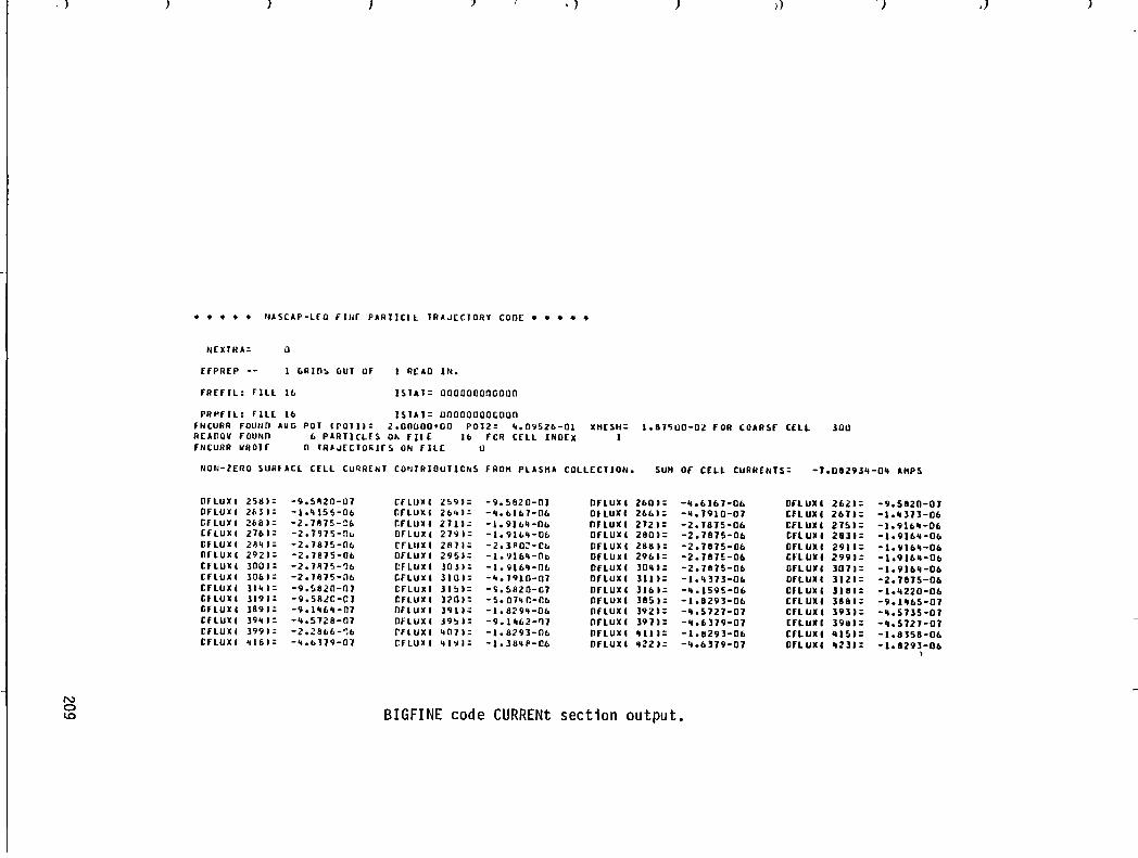
\ )
N o ~
J ') .) ) ») 'J ,) )
• • • •• NASCAP-L£O flW£ PARTICLL TRAJ[CIORY CODE •••••
N£XTRA: 0
ffPREP -- GRIO:' ClUJ OF 1 R[AO IN.
fR£fIL: flLl 11. ISTAT= 000000000000
PRl1fIL: fILL 16 ISIAT= OOOOOOOOCOOO fNCURR FOUNn AVe. POT IPOTII: 2.00000000 POI2: ~.n952b-Ol XHESH: 1.81~OO-02 fOR COARSf CELL 100 REAOQV fOUNn I. PARTICLES O~ filE 16 feR CtLL INorx I fNCURR WROlf 0 TR'JECTO~lrs ON fiLE U
NON-ZERO SURfACE CELL CUqRENT CO~IRIBUIICNS fROH PLASHA COLLECTION. SUH Of CELL CURRENTS: -1.08293~-0~ AHPS
OfLUXI 25111: -9.5~20-01 CfLUXI 2591= -9.5820-01 OHuxa 2601 -'1.1>161-01. OHUka 2621 -9.5820-0J DHUXI 21.31: -1'''155-06 OHUXI 2641: -~.6Ibl-0b Of LUX I 26b I - ... 1910-01 CHUXI 2(1) -1.'1313-06 tHUx I 21.8 1= -2.1815-~6 CHUX 2111: -1.916~-O6 OHUX I 2721 -2.1815-06 ULUXI 2151 -1.916'1-06 [fLUXI 2nl: -2.791S-0 .. OHUX 2HI: -1.9h"-Ob OHUX I 280 I -2.1815-06 CflUKI 28]1 -1.9Ib~-06 OHUXI 2e", -2.1815-01> rHUx 2811= -2.1~0::'-Cb OHUX I 28111 -2.1815-111. OHUKI 2911 -1.<,/16"-01. OHUXI 2921 -2.lelS-06 OHUX 2951= -1.911."-0 .. OHuxl 291.1 -2.1815-01. CHIlXI 2991 -1.911."-06 tHux I laO I -2.1~15-':lb eHUX 301l: -1.916"-01. OHUXI 30'" -2.1815-06 OfL UX I lOll -1.916"-01. CHux I 30£.1 -2.181S-nl> tHux 310 I: -".1910-01 OfLUXI 311 , -1."313-01. Of lUX I 3121 -2.1815-06 tHUx I 314' -9.5820-01 tHux 31!> I: -~.5820-01 OflUXI 311.1 -'1.1595-06 CHUXI lUI -1.'1220-01. Ofluxa 3191 -9.S8le-Ol tHux HO'= - 5.014 r.-nb OHUX I 385, -1.8293-06 Cflllxl 3881 -9 .... 1.5-01 OHUXI 3891 -9.1"6~-Ol OHUX 3911= -1.1129"-01. OHUXI 3921 -".5121-01 CHUXI 3931 - ... 5735-0J eHUx I 39~ I -'1.5128-01 OHUX J9~1= -~.1~62-'11 OrLUX I 3911 -'I.6319-0J [fluxa 39111 -'1.5121-01 tnulIl 1991 -Z.28bt-'1b rHUX ~01l : -1.8291-01> OHUXI ""1 -1.11293-06 Cfl UX I '115' -1.8358-01. CHUXI ~II)J - ... b119-01 eHUx 'I1'lI1= -1.18"P-Cb OflUXI '1221 -'1.1.319-01 DHUXI '1211 -1.8293-06
\
BIGFINE code CURRENt section output.
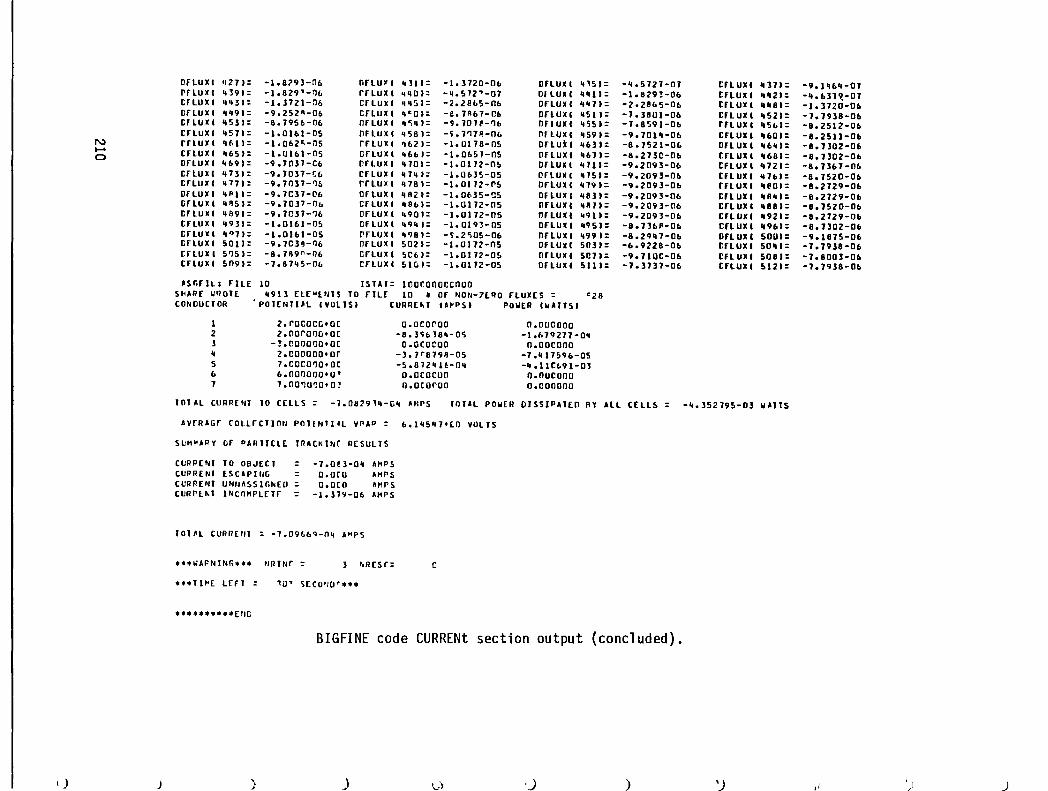
\)
N ...... o
J
OflUX IIZ7' -1.8?93-0b nflU' ! ~H ,: -1.3720-010 enuxi ~lS' -q.5727-07 cnUX! 1137' I'r LU X ~39' -1.82'1'-:)6 rfLUXI "qO': -~.572~-O7 OILUXI q"I' -1.8Z9~-Ob CfLUX! .... 2' efLUX ""3' -103721-06 CfLUXI ~"5': -'.l8bs-nb enUX! 'IH' -2.28105-010 trLuxl 'Iq8' onux 1I~9': -9.252~-06 CfLUXI 11<0': -e. Hb7-1l6 onuxi 'lSI' -7.l8UI-Ob efLUX! .. 52': tHUx .. 53': -8.7956-06 Of LUX! ~~II': -9.10U-'16 orlUX! 'ISS, -7.8591-010 rnUX! .. St.,: [fLUX 1157': -1.0161-05 OflUX I "58': -~ .7'1lR-Ob onuxi "S9'= -9.701~-06 CfLUXI 1160'= rnux "1>1': -1.062"-:)S rfLUX! '162': -1.UI18-0S onul! I .. 631 = -8.7521-01. (lnUXI "6~'= CflUX ~65': -1.0161-0S "fLUX! 1166': -1.06SJ-OS OHUXI 11611= -8.2130-06 tFLUXI '168': enux "69': -9.70ll-C6 rfLUX! ~JO': -1.0112-05 onUX! Iflll= -9.2093-06 CfLUXI .. 72': cnux '173': -9.70ll-G6 CflUXI 'Il~': -1.063S-05 onuxi illS': -9.2093-06 CFlUXI '176'= eflUX ~ 771: -9.7031-% "rLuxl '118': -I. UI12-I'S OrLUX! ~79'= -9.2093-06 rFL UX I .. eo,: OHUl( ~~ I': -9.7C37-06 OHUXI 'lA,': -1.0635-!lS efluxi 'I811: -9.2093-06 CfLUXI "S'l' IirLUXI ~~5 ,: -9.70]7-00 efLUXI 'Ie6'= -1.U172-0S nFluxi IIA7I= -9.2093-06 enux! '188' CrLUXI "89': -9.l0ll-'l6 efluxi 1190': -1.0112-05 OflUX I '191': -9.2093-06 cnUX! 1192' trLuxl '19]1: -1.0161-05 CHUXI 1111",= -1.0193-05 OHUXI '195': -8.736P-Ob ULUXI .. 96' CrLUXI .. '171: -1.0161-05 rfLUX I '1.,8': -~.2C;US-06 onuxi '199'= -8.29"7-010 OfLUXI SOD. eflUXI 5011: -9.70]9-116 nfLuxl S02': -1.UI72-05 OHUXI 5031: -6.9228-06 UlUXI 50 .. , CrLUXI5'15': -8.JA9~-06 crLuxl SCb': -1.0112-0S onuxi 5011= -9.7100-06 enuxi 508' erLUX I 5091: -7.87 .. 5-06 CflUXI 510': -1.0112-05 OrLUXI 511.: -7.3131-06 UlUXI 512'
'Sr,fIL: filE 10 ISlA': 100conoccooo SIiAP£ WIlOTE "913 [LENl~TS TO fIL£ 10 • Of NON-7lAO fLUXES : <28 CONDUCTOR 'POl£NTHL IVOllS' CURREIIT !A~PS , POWER IWAlTS'
1 2.rococc;·oc o.ocoroo 0.000000 2 2.(lOrOI10+or -8ol~bl8_-0o; -I .f> l'1277 - Oq 3 -!.COOOCO+OC o.aeocoo n.nocnno 'I 2.CODOOQ+or -3.7 r S79A-OS -7.q 175'16-05 5 7.COCO~0+OC -S.872QH-0'l -q .lICI.91-0] b 6.0UOOOO+0· O.OCOCUO a.ouconu 7 7.00'lU~0·0~ o.oeol'oo 0.000000
TOTAL CURRENT '0 CELLS: -1.0829l'l-IiQ .Mrs 'CTAL POWER DISSIPATED RY All CELLS = -q.352795-03 WATTS
AvrR.Gf rOLLrCTIon POTINTI8L VPAP : 6.IQS"7.(O VOLTS
SUH~APY or PARTICLE TRACK INC R(SULTS
CURPENT TO OBJECT : -1.0e]-Oq AIIPS CUPREN' lS C. P JIll; = o.oro .Hrs CURRENT UNn~SSIr,NEO = o.oeo AHrs CURrl t.T INCOHPL£lr = -lol711-0b AHPS
TOTAL CURnE"T : -7.09669-0~ AMPS
••• WAPNING... NRINr: 3 t.REsr: c
.. nl"E LCfT lOt sEeO'IO ••••
• • ••••• • •• [lIC;
BIGFINE code CURRENt section output (concluded).
) J \.,) I) ) 'J
-9.1116~-07
-".637~-01 -1.ll20-0b -7.7938-01. -8.2512-06 -8.2511-06 -8.7302-06 -8.7302-06 -8.7367-01. -8.7520-06 -8.2129-06 -8.2129-06 -8.7S20-06 -8.2129-06 -8.7302-06 -9.1875-06 -7.7938-06 -7.8003-06 -7.7938-06
,I ) )
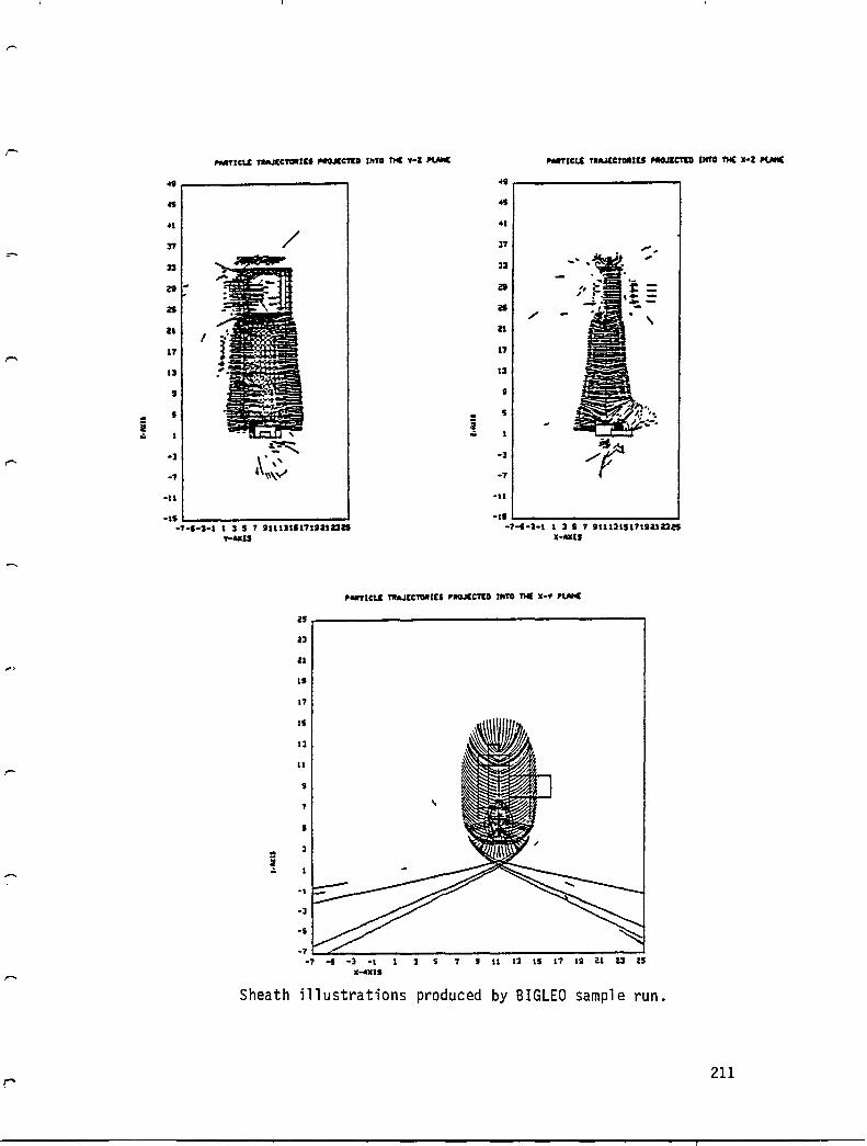
I'MTICU: TllAJECTOII1U PIIOJECTU I"TO TIC V-I PUIC I'MTICI.I TlAJlCTOIIIES ~ INTO M x-Z I'UIC
., .,
.1 .s
.1 .1
37 / 17
""' 31 31
2t~ at
ZI .,,-ZI
H II I
17 17
13 13
, , - s
! -] /if -7
- 5
i .:.
-3 ~':"'" ~ . r-- . '
-1 ' ""~ -II -II
-11
-ISL-____________________ ~
-1-5-3-1 1 1 S 7 '1l131111l1lUUS -1-1-3-1 1 1 S 7 '1l121UlI11I21JS Y-MIS X-AXIS
,......
is
2l
is
I'
17
15
Il
II
, 1
S
- 1
~ -l
-3
-5
-7 -7 -s -3 -1 5 7 , II 13 15 17 It U 2l 25
lC-AXIS
Sheath illustrations produced by BIGLEO sample run.
211 r

212

-.
(
APPENDIX A
NASCAP BIBLIOGRAPHY
We provide here a list of publications referencing the NASCAP and NASCAP/LEO computer codes. For the reader's convenience, we have separated the major S-CUBED reports (which collectively provide thorough NASCAP documentation) from articles published in technical journals and conference proceedings. Numerous monthly, topical, and interim reports and technical memoranda from S-CUBED and NASA/Lewis Research Center have been intentionally omitted. The authors I apologize for any other omissions or inaccuracies.
S-CUBED Reports
Katz, I., D. E. Parks, M. J. Mandell, J. M. Harvey, D. H. Brownell, S. S. Wang and M. Rotenberg, "A Three Dimensional Dynamic Study of Electrostatic Charging in Materials," NASA CR-135256, August 1977.
Mandell, M. J., J. M. Harvey and 1. Katz, "NASCAP User's Manual ," NASA CR-135259, August 1977.
Cassidy, J. J., "NASCAP User's Manual - 1978," NASA CR-159417, August 1978.
Katz, I., J. J. Cassidy, M. J. Mandell, G. W. Schnuelle, P. G. Steen, D. E. Parks, M. Rotenberg and J. H. Alexander, "Extension, Validation and Application of the NASCAP Code," NASA CR-159595, January 1979.
Stannard, P. R., I. Katz, M. J. Mandell, J. J. Cassidy, D. E. Parks, M. Rotenberg and P. G. Steen, "Analysis of the Charging of the SCATHA (P78-2) Satellite," NASA CR-165348, December 1980.
Katz, I., J. J. Cassidy, M. J. Mandell, D. E. Parks, G. W. Schnuelle, P. R. Stannard and P. G. Steen, "Additional Application of the NASCAP Code, Vol ume I: NASCAP Extension, II NASA CR-165349, February 1981.
Katz, I., J. J. Cassidy, M. J. Mandell, D. E. Parks, G. W. Schnuelle, P. R. Stannard and P. G. Steen, "Additional Application of the NASCAP Code, Volume II: SEPS, Ion Thruster Neutralization and Electrostatic Antenna Model, II NASA CR-165350, February 1981.
213
Mandell, M. J., 1. Katz and P. R. Stannard, "Additional Extensions to the NASCAP Computer Code, Vol ume I, II NASA CR-167855, October 1981.
Stannard, P. R., I. Katz and M. J. Mandell, "Additional Extensions to the NASCAP Computer Code, Volume II," NASA CR-167856, February 1982.
Mandell, M. J. and D. L. Cooke, "Additional Extensions to the NASCAP Computer Code, Volume III," NASA CR-167857, August 1981.
Published Papers
Katz, I., D. E. Parks, M. J. Mandell, J. M. Harvey, D. H. Brownell, S. S. Wang and M. Rotenberg, "A Three Dimensional Dynamic Study of Electrostatic Charging in Materials," NASA CR-135256, August 1977.
Mandell, M. J., I. Katz, G. W. Schnuelle and P. G. Steen, liThe Decrease in Effective Photocurrents Due to Saddle Points in Electrostatic Potentials Near Differentially Charged Spacecraft, II IEEE Transactions on Nuclear Science, NS-25, p. 1313, 1978.
Katz, I., J. J. Cassidy, M. J. Mandell, G. W. Schnuelle, P. G. Steen and J. C. Roche, liThe Capabil ities of the NASA Charging Analyzer Program," sgacecraft Charring Technology-1978, NASA CP-2071, AFGL-TR-79- 082, p. 101, 979.
Mandell, M. J., 1. Katz and G. W. Schnuelle, "Photoelectron Charge Density and Transport Near Differentially Charged Spacecraft, II IEEE Transactions on Nuclear Science, NS-26, p. 5107, 1979.
O'Donnell, E. E., "Spacecraft Charging Modeling Development and Validation Study," Spacecraft Charging Technology-1978, p. 797, 1979.
Roche, J. C. and C. K. Purvis, "Comparison of NASCAP Predictions with Experimental Data," s~acecraft Charging Technology-1978, NASA CP-2071, AFGL-TR-79-0082, p. 1 4, 1979.
Schnuelle, G. W., D. E. Parks, I. Katz, M. J. Mandell, P. G. Steen, J. J. Cassidy and A. G. Rubin, "Charging Analysis of the SCATHA Satellite," sbacecraft Char,ing Technology-1978, NASA CP-2071, AFGL-TR-79-00 2, p. 123, 19 9.
Stevens, N. J. and J. C. Roche, "NASCAP Modeling of EnvironmentalCharging-Induced Discharges in Satellites," IEEE Transactions on Nuclear Science, NS-26, p. 5112, 1979.
Mandell, M. J., 1. Katz and G. W. Schnuelle, liThe Effect of Solar Array Voltage Patterns on Plasma Power Losses," IEEE Transactions on Nuclear Science, NS-27, p. 1797, 1980.
214
.... I
....
Olsen, R. C., "Differential and Active Charging Results from the ATS Spacecraft. II University of California (San Diego) Ph.D. Dissertation, 1980.
Purvis, C. K., "Configuration Effects on Satellite Charging Response," AlAA Paper No. 80-0040, 1980.
Rubin, A. G., I. Katz, M. J. Mandell, G. W. Schnuelle, P. G. Steen, D. E. Parks and J. J. Cassidy, "A Three-Dimensional Spacecraft Charging Computer Code," H. B. Garrett and C. P. Pike, editors, Space Systems and Their Interaction with Earth1s Space Environment, New York, AlAA, 1980.
Stevens, N. J., "Model ing of Environmentally Induced Di scharges in Geosynchronous Sate11ites," IEEE Transactions on Nuclear Science, NS-27, p. 1792, 1980.
Katz, I., M. J. Mandell, G. W. Schnue11e, D. E. Parks and P. G. Steen, "Plasma Collection by High-Voltage Spacecraft in Low Earth Orbit," Journal of Spacecraft and Rockets, ~, p. 79, 1981.
Mandell, M. J., I. Katz and D. E. Parks, "NASCAP Simulation of Laboratory Spacecraft Charging Tests Using Multiple Electron Guns,1I IEEE Transactions on Nuclear Science, NS-28, p. 4568, 1981.
Newell, D. M. and W. E. Waters, IISpacecraft Charge Protection of Large 3-Axis Stabilized Communications Satellites-INTELSAT V,II IEEE Transactions on Nuclear Science, NS-28, p. 4505, 1981.
Olsen, R. C., C. E. McIlwain and E. C. Whipple, Jr., "Observations of Differential Charging Effects on ATS-6, II Journal of Geophysical Research, 86, p. 6809, 1981.
Olsen, R. C., IIModification of Spacecraft Potentials by Thermal Electron Emission on ATS-5,1I Journal of Spacecraft and Rockets, 18, p. 527, 1981. --
Purvis, C. K. and J. V. Staskus, IISSPM Charging Response: Comparison of Ground Test and Flight Data to NASCAP Predictions for Eclipse Conditions,1I Spacecraft Charging Technology-1980, NASA CP-2182, p. 592, 1981.
Rubin, A. G., H. A. Cohen, D. A. Hardy, M. F. Tautz and N. A. Saflekos, IIComputer Simulation of Spacecraft Charging on SCATHA,II Spacecraft Charging Technology-1980, NASA CP-2182, p. 632, 1981.
Saflekos, N. A., M. F. Tautz, A. G. Rubin, D. A. Hardy and P. M. Mizera, IIThree Dimensional Analysis of Charging Events on Days 87, and 114, 1979 from SCATHA,II Spacecraft Charging Technology-1980, NASA CP-2182, p. 608, 1981.
215

Sanders, N. L. and G. T. Inouye, "NASCAP Charging Calculations for a Synchronous Orbit Satell ite, II Spacecraft Charging Technology-1980, NASA CP-2182, p. 684, 1981.
Schnuelle, G. W., P. R. Stannard, I. Katz and M. J. Mandell, "Simulation of the Charging Response of the SCATHA (P78-2) Satellite," Spacecraft Charging Technology-1980, NASA CP-2182, p. 580, 1981.
Stang, D. B. and C. K. Purvis, "Comparison of NASCAP Modeling Results With Lumped-Circuit Analysis," Spacecraft Charging Technology-1980, NASA CP-2182, p. 665, 1981.
Stannard, P. R., I. Katz and D. E. Parks, "Bootstrap Charging of Surfaces Composed of Multiple Materials," IEEE Transactions on Nuclear Science, NS-28, p. 4563, 1981.
Stannard, P. R., G. W. Schnuelle, I. Katz and M. J. Mandell, "Representation and Material Charging Response of GEO Plasma Environments," Spacecraft Charging Technology-1980, NASA CP-2182, p. 560, 1981.
Staskus, J. V. and J. C. Roche, "Testing of a Spacecraft Model in a Combined Environment Simulator," IEEE Transactions on Nuclear Science, NS-28, p. 4509, 1981.
Stevens, N. J., "Use of Chargi ng Con tro 1 Gu i de 1 i nes for Geosynchronous Satell ite Design Studies," Spacecraft Charging Technology-1980, NASA CP-2182, p. 789, 1981.
Stevens, N. J., "Review of Biased Solar ArraY-Plasma Interaction Studies, II AIM Paper No. 81-0738, 1981.
Stevens, N. J., H. E. Mills and L. Orange, "Voltage Gradients in Solar Array Cavities as Possible Breakdown Sites in Spacecraft-Charging Induced Discharges," IEEE Transactions on Nuclear Science, NS-28, p. 4558, 1981.
Stannard, P. R., I. Katz, L. Gedeon, J. C. Roche, A. G. Rubin and M. F. Tautz, "Validation of the NASCAP Model Using Spaceflight Data," AIM 82-0269, 1982.
216

APPENDIX B
NASCAP SIMULATION OF LABORATORY SPACECRAFT CHARGING TESTS USING MULTIPLE ELECTRON GUNS
M. J. Mandell, I. Katz and D. E. Parks
IEEE Transactions on Nuclear Science, NS-28, p. 4568, 1981.
217

218
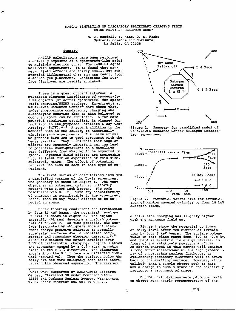
r
-I
NASCAP SIMULATION OF LABORATORY SPACECRAFT CHARGING TESTS USING MULTIPLE ELECTRON GUNS·
M. J. Mandell, I. Katz, D. E. Parks Systems, SC1ence and Software
La Jolla, CA 92038
Summary
NASCAP calculat10ns have been performed s1mulat1ng exposure of a spacecraft-11ke model to multiple electron guns. The results agree well with exper1ment. It 1S found that magnet1c field effects are fa1rly small, but substantial different1al charg1ng can result from electron gun placement. Cond1t1ons for surface flashover are readily achieved.
There is a great current interest in mult1beam electron irradiat10n of spacecraftl1ke obJects (or actual spacecraft) for spacecraft charg1ng/SGEMP stud1rs. Experiments at NASA/Lew1s Research Center have shown that, under appropr1ate cond1t1ons, charg1ng and d1scharg1ng behav10r ak1n to that be11eved to occur 1n space can be s1mulated. A far more powerful s1mulat1on capabi11ty is planned for 1nclus1on 1n the p~oposed Satel11te X-Ray Test Fac1l1ty (SXTF).2,3 A recent addition to the NASCAP4 code is the ab1l1ty to numerically simulate such exper1ments. The calculations we present here are 1n good agreement with the LeW1S results. They 1llustrate that angular effects are extremely 1mportant and can lead to potent1al conf1gurat1ons on a satel11te very d1fferent from what would be expected 1n space. Magnet1c f1eld effects are not1ceable but, at least for an exper1ment of th1S S1ze, relat1vely m1nor. The effect of potent1al barr1ers can also be seen 1n th1S type of experiment.
The f1rst ser1es of calculat10ns 1nvolved a s1mp11fied verS10n of the Lewis exper1ment. The geometry 1S shown 1n F1gure 1. The test obJect 1S an octagonal cy11nder un1formly covered w1th 0.005 1nch kapton. The code resolut1on was 0.1 m. Thus any nonun1form1ty of charg1ng 1S atrr1butable to the exper1ment rather than to any "real" effects to be expected 1n space.
Under float1ng cond1t1ons and 1rradiat1on by four 10 ~eV beams, the potent1al develops 1n t1me as shown 1n F1gure 2. The obJect 1n1t1ally (~l sec) develops a un1form potent1al of ~-7200 v. As t1me proceeds, the surface irrad1ated by obliquely inc1dent electrons charge pos1t1ve relat1ve to normally 1rrad1ated surfaces due to 1ncreased back-
6 scatter and secondary electron em1ss10n. 5 , After S1X m1nutes the obJect develops over 2 kV of d1fferent1al charg1ng. F1gure 3 shows the asymmetry caused by a 0.7 gauss magnet1c f1eld 1n the 0 1 r d1rect1on. The electrons 1nc1dent on the 0 1 1 face are deflected downward (toward -x). Thus the surfaces below the belly are h1t more ob11quely than those above, caus1ng the observed asymmetry. The maX1mum
* Th1S work supported by NASA/Lew1s Research Center, Cleveland OH under Contract NAS3-22536 and Defense Nuclear Agency, Wash1ngton, D. C. under Contract DNA 001-79-C-0079.
1
GUN
~--.. \ -... -....... \ --.. \ ------
GUN
/ \ 30° Cone ---
\~Half-angle ~~O \ B
\
1 0 Face
/ GUN
\ \ \ \
\ \ \
o 1 1 Face
" GUN
Figure 1. Geometry for s1mplif1ed model of NASA/Lew1s Research Center mult1gun 1rrad1at10n exper1ment.
V -8000 Potential versus Time
-6000
10 keV Beams _5 ~ 0
-B'" 0 -2000~~ _________ ~ ______ ~~ ______ ~~ ___ ~
1.0 10 100 0.1 Time (sec)
F1gure 2. Potent1al versus t1me for 1rrad1at10n of kapton covered cy11nder by four 10 keV electron beams.
d1fferent1al charging was s11ghtly h1gher W1th the magnet1c f1eld on.
Figure 4 shows the potential contours at belly level after ten m1nutes of 1rradiat10n by four 6 keV beams. The surface potent1als 1n th1S plane range from -5.0 to -2.8 kV, and there 1S electr1c f1eld s1gn reversal 1n front of the relat1vely pos1t1ve surfaces. An obJect charged 1n th1s manner w1ll exn1b1t strong SGEMP enhancement w1th a h1gh probab1l-1ty of synerg1st1c surface flashover, as avalanch1ng secondary electrons w11l be drawn back to the em1tt1ng surface. However, 1t 15 un11kely that a s1mple obJect such as ~~1S would charge to such a state 1n the relat1vely 1sotrop1c enV1ronment of space.
Further calculat10ns were performed w1th an obJect more nearly representat1ve of the
219
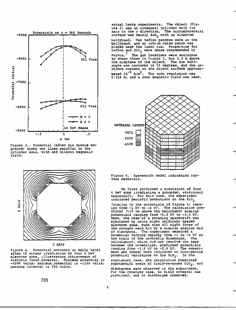
-9000 Potent1als at t .. 360 Seconds
I I I
I I I
-8000 I I I -III I
...a I ~
0 I > I ~ -7000 I co I ....
I ...a c I <II ...a I 0 I ~
~.¢X~~ -6000 Face I 010
I I
--0- B 0 I .. I
- B " 0
-5000 110, kt;V ,Be~, -.5 0 .5
x (m)
Figure 3. Poten~al (after S1X m1nute exposure) along two lines parallel to the cylinder ans, Wl. th and W1 thout magnetl.c held.
Y AXIS
Fl.gure 4. Potentl.al contours at belly level after 10 m1nute l.rradl.atl.on by four 6 keV electron guns, l.llustratl.nq achl.evement of electr~c field reversal. Minimum potentl.al is -4996 volts: maXl.mum potential l.S -1149 volts: contour interval l.S ZOO volts.
220
Z
actual Lewis experiments. The obJect (Figure 5) was an octagonal cyll.nder Wl.th its axl.S in the y direction. The cl.rcumferentl.al surface was mal.nly Sl.0Z with an aluminum bellyband. Two teflon patches were on the bellyband, and an l.ndl.um oxide patch was placed near the lower rl.m. Propertl.es for teflon and SiOZ were those recommended by purvl.s. 7 The gun locations were analogous to those shown in Fl.gure 1, but 0.3 m above the IUl.dplane of the object. The gun halfangle was narrowed to 15 degrees, and the l.ncident current at the obJect surface appron-mated 10-5 A/mZ. The code resolutl.on was 0.114 m, and a zero magnetic field was used.
TEFL 0 SIOZ IIITI ALUM El
Figure 5. Spacecraft model l.ndl.catl.ng surface materl.als.
We first performed a sl.mulatl.on of four 6 keV guns l.rradl.atl.ng a grounded, statl.onary spacecraft. For thl.S case, the experl.ment l.ndl.cated perl.odic potentl.als on the Sl.0Z
(sl.m1lar to the potentl.als of Figure 4) rangl.ng from -1 kV to -4 kV. The calculatl.on predicted (~l5 em above the bellyband) sl.IUl.lar potentl.als ranging from -O.B kV to -3.4 kV. Next, the case of a rota~ng spacecraft was simulated by using eight uniformly spaced electron guns, such that all eight faces of the octagon were hl. t by a sl.IUl.lar angular m1X of electrons. The experl.ment measured a potentl.al varyl.ng rapl.dly from -1 to -4 kV on the scale of the coversll.p dl.mensl.on. The calculatl.on, whl.ch dl.d not resolve the gaps between the coversll.ps, predl.cted potentl.als rangl.ng from -l.B kV to -Z.O kV. The experl.ment and theory both l.ndl.cated no long-perl.od potentl.al varl.atl.ons on the Sl.0Z. In the statl.onary case, the calculatl.on predl.cted substantl.al areas of fl.eld-reversed Sl.0Z' and discharges were observed l.n the experl.ment. For the rotatl.ng case, no fl.eld reversal was predl.cted, and no dl.scharges observed.
-,

r
..
Finally, we calculated the charg~ng of the model spacecraft under float~ng cond~tJ.ons exposed to four b~-energy guns. The gun energies were set to 10 keV and 20 keV, each beam hav~ng intens~ty ~10-5 A/m2 at the uncharged surface. The potent~al versus t~me is shown ~n Figure 6. For th~s case, the h~gh secondary e~ssion and backscatter coeffic~ents for obliquely inc~dent electrons stopped the rap~d charg~ng process at about -7.6 kV. (W~th the 10 keV beams alone, the potent~al reached -6 kV.) (Recall that the kapton cylinder, desp~te low secondary and backscatter coeffic~ents, charged only to -7.2 kV in four 10 keV beams.) At th~s potent~al the ~ncident flux from the low energy beams is about 40 percent of the flux from the high energy beams. For those surfaces wh~ch continue to charge negat~vely, the low energy beam ~s attenuated further. After n~ne ~nutes, surface potentials range from -5.3 to -9.1 kV, and about 20 percent of the surface is ~n a f~eld-reversal condition. As the metall~c substrate contl.nues to charge negat~vely, the amount of f~eldreversed surface ~ncreases. The "bootstrap effect"8 eventually causes the entire spacecraft to drop below -10 kV, repell~g completely the lower energy beam. After about a half hour, equ~libr~um is reached at about -17 kV.
_10 4
-9000.
-8000
-7000
:> -6000
-5000
-4000
-3000 0.02 0.1 1.0 10.0 100 1000
Time (sec) F~gure 6. Potent~al versus t1me for spacecraft model ~rrad~ated by four b~-energy (10 and 20 keV) electron guns. Cell 92 ~s a teflon cellon the bellyband w~th r 0 1 surface normal. Cell 8 ~s an S~02 cell with rOO normal near the aft (bottom) end.
l'1e conclude that great care must be taken ~n des1gn and 1nterpretat~on of satell~te ~rrad~ation experiments. Several electron beams ~n a vacuum tank need not prov1de a good three-d1mens10nal s~m~lat~on of a hot plasma. The calculat~ons presented here agree well w~th recent laboratory exper1-mentsl that showed several thousand volts of d1fferent1al charg~ng due to electron beam placement. Our calculat~ons have also shown that the f1eld reversal cond~t~ons necessary for surface flashover may be caused by these asymmetr~es. Th~s ~s 1n contrast to prev~ously observed and calculated results for the ~rrad1atl.on of planar samples. Although
3
th~s type of asymmetry is not expected in space, s~~lar field reversal conditions can occur due to mater~al differences 8 or associated with art~f~cial charg~ng.9 Analysis of SCATHA data shows several occurrences of field-reversal effects. 10 Since the recent three-d1mensional laboratory exper1ments exh1bited discharges s~~lar to those observed in space, this flashover mechanism may be respons1ble for arc1ng observed on spacecraft.
References
1. Staskus, J. V. and J. C. Roche, "Test1ng of a Spacecraft Model ~n a Comb~ned EnV1ronment S1mulator," 1981 IEEE-NSRE Conference, Paper I-3.
2. Flanagan, T. M., M. J. Treadaway and R. Denson, "Strawman Plasma Environment Simulat~on Req~rements for SXTF," JAYCOR Report 200-80-223/2066 (1980).
3. Halverson, W. D., "Eng~neer~g Assessment of the SXTF Spacecraft Charg~ng Capab111ty," SPIRE Report (1980).
4. Katz, I., J. J. Cass~dy, M. J. Mandell, G. W. Schnuelle and P. G. Steen, "The Capabil~tJ.es of the NASA Charg1ng Analyzer Program," presented at OSAF/NASA Spacecraft Charg1ng Technology Conference (1978).
5. Katz, I., D. E. Parks, M. J. Mandell, J. M. Harvey, D. H. Brownell, Jr., S. S. Wang and M. Rotenberg, "A Three D~mens~onal Dyn~c Study of Electrostat1c Charg1ng ~n Mater~als," NASA CR-135256, August 1977.
6. Saleh1, M. and E. A. F11nn, "Dependence of Secondary-Electron Emiss10n from Amorphous Mater1als on Pr1mary Angle of Inc1dence," J. Appl. Phys. g, 994 (1981).
7. PUrv1S, C. K. and J. V. Staskus, "SCATHA SSPM Charg~ng Response: NASCAP Predict10ns Compared to Data," Spacecraft Charg1ng Technology, 1980, NASA CP-2182 (1981) •
8. Stannard, P. R. and I. Katz, "Bootstrap" Charg1ng of Surfaces Composed of Mult1ple Mater1als," 1981 IEEE-NSRE Conference, Paper I-12.
9. Katz, I. and M. J. Mandell, to be pubhShed.
10. Stannard, P. R., to be published.
221

"
222
APPENDIX C
"BOOTSTRAP" CHARGING OF SURFACES COMPOSED OF MULTIPLE MATERIALS
P. R. Stannard, I. Katz and D. E. Parks
IEEE Transactions on Nuclear Science, NS-28, p. 4563, 1981.
223
224

.,
"BOOTSTRAP" CHARGING OF SURFACES COMPOSED OF MULTIPLE MATERIALS*
P. R. Stannard, I. Katz and D. E. Parks Systems, Science and Software
P. O. Box 1620, La Jolla, CA 92038
Abstract
We examine the charging of a checkerboard array of two materials, only one of which tends to acquire a negative potential alone, using the NASA Charging Analyzer Program (NASCAP). The influence of the charging material's field causes the otherwise "non-charging" material to acquire a negative potential due to the suppression of its secondary emission ("bootstrap" charging). The NASCAP predictions for the equilibrium potential difference between the two materials are compared to results based on an analytical model.
Introducti on
In the presence of a plasma, exposed surfaces of both insulators and conductors collect a current of incident charged particles and may acquire an electrostatic potent1al. The tendency to charge in this way is different for different mater1als since the net current collected depends on the nature of the surface as well as the plasma parameters. While the latter determine the magnitude of the primary incident electron and ion currents, ie and iion' processes such as secondary electron emission, backscatter and (1n the presence of sunlight) photoemission also make a contribution to the net current:
inet ~ 1ion - 1e
+ ie(6+~) - iion 6ion + ip•
In th1S equation 6 and 6iQn are the secondary electron emission yields for electron and 10n impact at the material surface respectively, ~ is the electron backscatter Y1eld and ip the photocurrent emitted.
The values of the yields for these processes depend strongly on the nature of the surface materia1.El] Satellites orb1ting at high altitude are bathed 1n plasmas with temperatures 1n thg kilOvolt range and dens1ties on the order of 10 m-. The many different mater1als that comprise the surface of a satellite may respond differently to th1s environment, leading to the bU11dup of substantial (-several kV) d1fferential potentials between neighbor1ng surfaces, and even damaging discharges.
As a result of both experimental observation and numerical modeling of spacecraft charging it has become evident that the charging behavior of an exposed surface depends on the response of[lts]neighbors as well as Just its own properties. Z,J In this study we investigate this phenomenon and examine the charging response of a slab composed of a checkerboard-like arrangement of two mater1als (Figure 1), and compare it to the response of each material alone.
* This work supported by NASA/Lew1s Research Center, Cleveland, OH, under_Contract NAS3-22536, and U. S. Air Force Geophysics Laboratory, Hanscom A1r Force Base, MA.
1
--" ~e.g., 0.1 m
~MAn
OMAT2
Figure 1. Checkerboard slab of two different materials, MAn and MAT2.
"Chargi ng" and "Non-chargi ng" Materi al s
For a given pTasma environment. s1m11ar to those encountered at high earth orbit, a pure sample of a material will either acquire a s1gnificant potential negative with respect to the plasma, or remain essentially neutral. Large positive potentials can never be achieved by natural charg1ng (i.e., in the absence of electron emitters or other outside biases). To understand this consider how a surface reaches its equilibrium potential. For a neutral plasma the incident electron current is much greater than the 10n current due to the mass difference between the two species. Hence there is a net flow of negative charge to the material and the surface begins to acquire a negative potential. The incident Current is opposed by the secondary electron current and photocurrent emitted from the surface. The surface w1l1 continue to charge negatively until its potential retards the 1ncident current sufficiently to exactly balance the emitted current giving a net flow of zero. This balance point 1S the equilibrium surface potential ~. Values of ~ may be many k110volts negative, or just a few volts pos1tive according to the magn1tude of the secondary emission yield for the material, and the intens1ty of illumination. If the emitted current initially exceeds the incident flow of negative charge the mater1al will tend to acquire a positive potential. However, because the energy of the emitted secondary and photoelectrons is only a few electron volts, once the potential reaches a positive value of sim11ar magnitude the emitted current is unable to escape and charg1ng stops. Thus all materials tend to stay within 2 or 3 volts from neutral in the presence of strong sunlight, where photoemiss10n dom1nates. In eclipse on the other hand, for a given set of plasma parameters, materials either charge rap1dly to significant negative potent1als or remain close to neutral according to their secondary emission yields. Those materials that do acqu1re a negative potential are desi gnated as "chargi ng" matern 1s and those that remain neutral are called "non-charging". Obviously this partition depends completely on the choice of plasma environment.
225

Simulation of Charging of a Checkerboard Array
To investigate the effect of neighboring materials on charging, the response of the object shown in Figure 1 to a 5 keY, 106 m-J electron! proton plasma was simulated using the NASA Charging ~nalyzer ~rogram (NASCAP). NASCAP is 'ihigli'ly sophisticated three-dimensional spacecraft charging code, capable of detailed representation of both objects and environments. A full descEigtion of its capabilities has been given elsewhere. 4J The NASCAP model assumes that both dielectric materials are present as thin films covering the same floating conductor. Bulk conductivity between the exposed surface and the conductor is taken into account by the code, but its magnitude is small compared to current collection from the plasma.
Three materials were chosen for study; kapton, teflon and solar cell coverglass ("solar"). The latter is a silicon dioxide glass with a MgF2 reflective coating. Of these materials only kapton charged in the environment chosen. The thicknesses and other material properties of these dielectrics covering the underlying conductor were chosen to correspondrtQ the values used on the SCATHA (P78-2) satellite.-2J In all but the last case the material patches were 0.1 m x 0.1 m. The computational grid was 3.5 m x 3.5 m in the plane of the slab and extended 7 m in the remaining (z) direction.
Four cases are discussed.
1. Both materials kapton, i.e., a pure kapton slab.
2. The first material kapton and the second "solar".
3. The first material kapton and the second teflon.
4. An expanded checkerboard model with 0.4 m x 0.4 m patches of kapton and solar.
In the first case the slab quickly (4 secs) charged to an equilibr,um potential of -3.67 kY for both the surface and the underlying conductor. In both of the remaining two cases the kapton surfaces began to charge negatively, but on a much longer timescale (l00 sees). The "non-charging" surfaces also began to charge, lagg,ng behind the kapton until the equilibrium was reached. At equ,librium kapton again had a potential of -3.67 kY but the underly,ng conductor and the re~a'ning surfaces reached a smaller potential. This is shown in Figure 2 for kapton and solar. Kapton and teflon behaved very similarly. To understand these results we must examine the local electric fields above the surface.
"Bootstrap" Charging
The charging of the otherwise "non-charging" teflon and solar ,n the presence of the strongly charging kapton is due to the suppress,on of secondary emission by the electric field above the surface. The potential contours across the surface as the kapton charges are shown schematically in Figure 3. The negative potential on the kapton p,atch influences the potential in front of the 'non-charging" patch causing a barrier or saddle point to fonn. Once the height of this barrier exceeds the energy of the secondary electrons (2 or 3 volts) they can no longer escape. The equ,librium potenti al for the "non-chargi ng" materi al is hence shifted from approximately zero to a much more negative potential and it too may begin to charge.
226 2
.-
0.0.----------------....
, -1.0 -\
\ \ \ \
"Solar" Cell Coverglass _____ _
Kapton ---
" ~ -2.0 '"
,~ .... c .. ...
-------------- ------~
-3.0
-4.0L-__ ~ ___ ~ ___ ~ __ ~ ___ ~
25 50 75 100 Time (sees)
Figure 2. Charging of kapton/solar cell coverglass, Checkerboard array.
-1.0 -1.0 -La
i -1. 6 Saddl e Point -1. 6 ~ I
'~f' ;\ ----:: :::---- A ~'\ ~-2~~ / ,,' // ~-2~~ \ ~ ~\I 1~~~~,\',~'.I"lt~i,"'~ ~""";;:=:-3?§1!/!I~; I'·iE_3.?;§,!1I ~
KAPTON TEflON KAPTON
Figure 3. Potential contours above the checkerboard surface with kapton fixed at -3 kV and teflon at -1 kV.
While in the absence of secondary emission both teflon and solar would charge to potentials much more negative than -3.67 kV, their potentials must lag behind that of the kapton for their secondary emission to remain suppressed. The extent to which their potential lags is determined mainly by the geometrical relationship between the kapton surface potent,al and the potential felt just above the "non-charging" surfaces. The properties of the non-charging surface can, in principle, playa role however. Since backscattered electrons have an energy similar to those incident they are not fully suppressed by the potential barrier and their yield is different for each mater,al. In addit,on, the proportion of the secondary electrons that escape depends on the overlap of the emission spectrum and the local retarding potential. While th,s proportion ,s close to zero, some secondaries do escape and this too may influence the final potential of the "non-charging" surfaces.
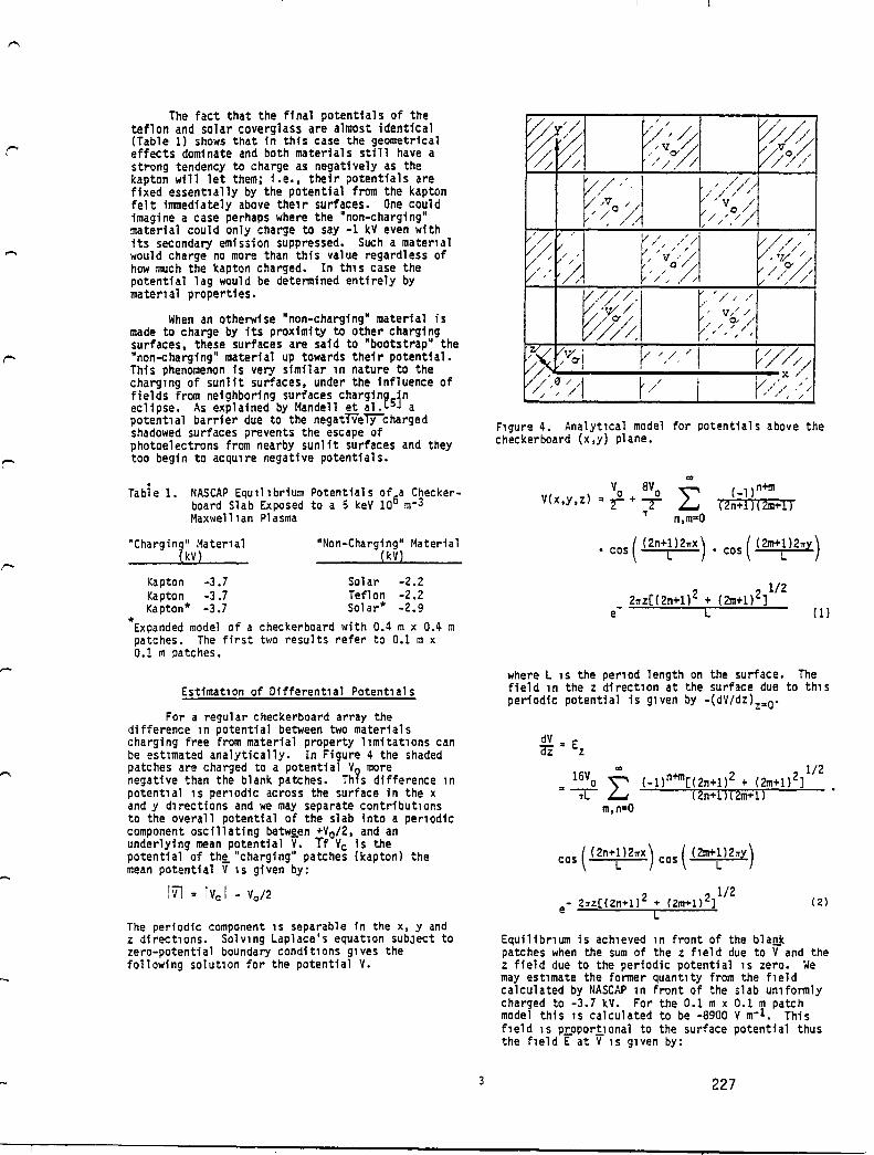
The fact that the final potentials of the teflon and solar coverglass are almost identical (Table 1) shows that in this case the geometrical effects dominate and both materials still have a strong tendency to charge as negatively as the kapton will let them; i.e., their potentials are fixed essent1ally by the potential from the kapton felt immediately above the1r surfaces. One could imagine a case perhaps where the "non-charging" material could only charge to say -1 kV even with its secondary emission suppressed. Such a mater1al would charge no more than this value regardless of how much the kapton charged. In th1s case the potential lag would be determined entirely by mater1al properties.
When an otherwise "non-charging" material is made to charge by its proximity to other charging surfaces, these surfaces are said to "bootstrap· the "non-charging" material up towards their potential. This phenomenon is very similar 1n nature to the charg1ng of sunlit surfaces, under the influence of fieldS from neighboring surfaces chargfnasjn eclipse. As explained by Mandell et al.[ j a potent1al barrier due to the negatTVer;y-charged shadowed surfaces prevents the escape of photoelectrons from nearby sunlit surfaces and they too begin to acqu1re negative potentials.
Tabie 1. NASCAP Equ1l1brium Potentials of6a Checkerboard Slab Exposed to a 5 keY 10 m-3 Maxwell1an Plasma
"Charging" Mater1al (kV)
"Non-Charging" Material (kV)
*
Kapton -3.7 Kapton -3.7 Kapton* -3.7
Sol ar -2.2 Teflon -2.2 Solar* -2.9
Expanded model of a checkerboard with 0.4 m x 0.4 m patches. The first two results refer to 0.1 m x 0.1 111 patches.
Estimat10n of Different1al Potent1als
For a regular checkerboard array the difference 1n potential between two materials charging free from material property llmitat10ns can be est1mated analytically. In Figure 4 the shaded patches are charged to a potential VQ more negative than the blank patches. Th1s difference 1n potent1al 1S per10dic across the surface in the x and y d1rections and we may separate contribut10ns to the overall potential of the slab into a per10dic component oscillating betw~en +Vo/2, and an underlying mean potential V. Tf Vc is the potential of th!t "charging" patches (kapton) the mean potential V 1S given by:
Iv! " IVe I - Vo/2
The periodic component 1S separable in the x, y and z direct1ons. Solvlng Laplace's equat10n subJect to zero-potential boundary condit1ons glves the following solut10n for the potential V.
3
F1gure 4. Analyt1cal model for potentials above the checkerboard (x,y) plane.
co
(_l)n+m L (2n+ll! 2m+1J n,m"O
(1)
where L 1S the per10d length on the surface. The field 1n the z direct10n at the surface due to th1s periodic potential is g1ven by -(dV/dZ)z"O.
dV - E Qz - z
1/2 (_1)n+m[(2n+1l 2 + (2m+l)2]
(2n+1) (2m+ll
(2)
Equilibr1um is ach1eved 1n front of the bla~k patches when the sum of the Z f1eld due to V and the Z field due to the periodic potential 1S zero. We may est1mate the former quant1ty from the f1eld calculated by NASCAP 1n front of the slab un1formly charged to -3.7 kV. For the 0.1 m x 0.1 m patch model this 15 calculated to be -8900 V m- 1• This f,eld 1S PLoporl1onal to the surface potential thus the f1eld E at V 1S glven by:
227

The field E~ due to the periodic potential is gfven by summing the convergent series in Eq. (2).
L • 0.2 m and so
Vo is the solution to the equation
EO + E a O. z
32.85 Vo - ( 3700 - .;) .mg.. 0
Vo = 260 volts
and
E - -8540 V m-1•
This differs considerably from the value of 1500 V predicted by NASCAP (Table 1). The source of this discrepancy lies in the crude spatial resolution of our slab model. As can be seen from (2) the periodic field Ez decreases exponentially with distance above the slab with a scale length L/2~1.r. NASCAP assumes only a linear decrease across each finite element zone. Thus unless the zone size is much smaller than the scale length NASCAP underestimates the field due to the periodic potential at the surface, compared to that predicted analytically, for the same potential drop across a zone. This is illustrated schematically in Figure 5. In the case of the 0.1 m x 0.1 m slab model the scale length is 0.02 m, five times smaller than the zone size. Hence NASCAP underestimates the field due to its charging neighbors 1mmediately in front of a blank patch and so requires a much larger potential drop across a zone than that predicted by the analytical model, to produce the same field at the surface. The larger potential drop across a zone can only occur by reducing the magnitude of the potential of the blank patches, i.e, by increasing the difference between the two surfaces VO' So NASCAP predicts a larger potential difference Vo than the analytical model.
This discrepancy in the value of Vo predicted by the two models should decrease as the ratio of zone size to scale length decreases. To test this hypothesiS an expanded model of the slab was constructed with 0.4 m x 0.4 m patches. The NASCAP results in Table 1 show a Vo value of 800 volts. The field in front of this expanded model uniformly charged to -3.7 kV is calculated to be -3700 V m-1• With this value the analytical model predicts Vo to be 425 V and agreement between the models is closer as expected.
228 4
V slJrfac
, ,
Actual Potential --- Profile ____ ..NASCAP Implied
Profil e •
~ ---------Vl~~ri;,? ... ~ Point ... , ~ " E '~ VI ,
~------------------~ ----Zone S1ze
Figure 5. Whlle NASCAP correctly estimates potent1als at the grid points, 1n th1S case it prov1des a poor estimate of behav10r within the first zone, and underestimates the slope (f1eld) at the surface.
Charging Timescales
The rate at which potential changes depends upon the rate of charge accumulation and the capacitance C of the system be1ng charged.
Cd • charge· inet dt
Given the same inet the charging rate depends on the inverse of the capacitance
dQl i net dt'-c-A circuit diagram of two dielectr1c surfaces covering a conductor is shown in Figure 6. There are two main sources of capacitance.
1. The small capacitances of any surface to infinity. (For a sphere these have the well known form C • 4~£0Ir.)
2. The much larger capaCitance between the two surfaces via the underlying conductor. (A small through space capacitance is also present. )
In series the inverse of capacitances are additive,
and initially the small capacitances dominate, causing rapld charging of all the surfaces and the underlYlng conductor together, until current balance for the whole object 1S achieved. The excess charge

--
i Small Capacitance to Infinity
Small Capacitwe Couplinq
Large Capacltive
T Coupling to Conductor
UnderlYlng Conductor
!
Figure 6. Circuit d1agram of two surfaces coupled Vla an underlYlng conductor.
on net emitting surfaces is then redistributed to absorbing surfaces and the large capacitances begin to charge. This occurs on a correspondingly slower timescale. Only as differential charging occurs in this way can suppression of secondary emission begin. Thus "bootstrap" charging occurs on a long differential charging tImescale (100 secs) dom1nated by the large capacItances. Charging of pure kapton, however, 1S determined only by the 1nitial small capacitance response and occurs on a much shorter (4 secs) timescale.
Conclusions
The most important conclusion from this study IS that regular arrays of different materials can charge according to their most charg1ng constituent, but on a considerably longer timescale. This may be most signIficant 1n modellng the response of solar arrays where the coverglass is typically noncharging and the grouting may be chargIng. In addition, comparison of NASCAP calculations with an analytical treatment shows the importance of sufficient finite element resolution in determining numerical accuracy.
To summarize we have shown that otherwise non-charging materials can be made to charge by their proximIty to charging surfaces on a fairly long tlmescale. This phenomenon arises from the suppression of secondary emiSSIon by the field derIved from the adjacent charging surface. The potential to which the "bootstrapped" surfaces charge 1S determined by geometric effects when their secondary-suppressed equll1brium potential exceeds the potential of the ne1ghboring charging surface. Otherwise only the secondary-suppressed equilibrium potential is reached.
5
1.
REFERENCES
Katz, 1., et!l.:., "A Three DimenSional Dynamic Study of ETectrostatic Charging in Materials" NASA CR-135256, August 1977. '
2. Stannard, P. R., et al., "Analysis of the Charging of the S~(P78-2) Satellite" Systems, Science and Software Final Repo;t SSS-R-81-4798, December 1980. '
3. Purvis, C. K., et al., ·Charging Rates of Metal-DielectriC-StrUctures," Spacecraft Charging Technology-1978, NASA Conference Publication 2071, AFGL-TR-79-0082, 1979.
4. Katz, I., $ al., "The Capabilities of the NASA Charglng-xnalyzer Program,· USAF/NASA Spacecraft Charging Technology Conference November 1978, AFGL TR-79-0082. '
5. Mandell, M. J., et al. "The Decrease in Effective Photocurrent~ Due to Saddle Points in Electrostatic Potentials Near Differentially Charged Spacecraft," IEEE Trans. on Nuc. SCi., Vol. NS-25, No.6 December 1978. '
229
230

APPENDIX D
FLUID MODEL OF PLASMA OUTSIDE A HOLLOW CATHODE NEUTRALIZER
D. E. Parks, M. J. Mandell and I. Katz
, To be published in Journal of Spacecraft and Rockets, 1982.
231

232

FLUID MODEL OF PLASMA OUTSIDE A HOLLOW CATHODE NEUTRALIZER D. E. Parks,* M. J. Mandell,** I. Katz,
Systems, Sc~ence and Software La Jolla, Cal~forn~a 92038
Abstract
The present study analyzes the capab11~ty of a flu1d model of electron transport to expla~n observed propert~es of the external plasma of a hollow cathode neutral~zer used to neutral~ze beams emerg1ng from lon thrusters. Calculat10ns reported here show that when the effect~ve col11-S10n frequency In such a model 1S near the plasma frequency, the result~ng electr1c potent1al and electron temperature var1at10ns are 1n qualitat1ve agreement W1th values measured ln the plume mode of the hollow cathode. Both theory and experiment show strong var1at10ns of temperature and potent~al wlth~n a few cent1meters of the cathode or1f1ce.
Nomenclature
E k1net1c ener~y of an electron t electr1c f1eld j net current dens~ty k Boltzmann's constant m electron mass n electron dens1ty p scalar electron pressure q magn~tude of electron charge '! heat flux ~ pos~t~on vector R col11s10nal drag force between elec
trons and ~ons T electron temperature u = v_ - 'i7+
AD 0 = T1 K
'J 'Je~ rJ
~ W
wp
dr~ft veloc~ty of electrons dr1ft veloc1ty of 10ns mean free path for pa1r col11s10ns between electrons Debye length kT plasma res~st~v~ty thermal conduct~v~ty of plasma effect~ve coll~s~on frequency electron-~on col11s1on frequency 'j-l electr~c potent~al frequency of osc~llatlon of fluctuat~ng f~eld electron plasma frequency
1. Introduction
The purpose of the present study lS to further exam~ne the capab~l~ty of a flu~d model of electron transport to expla~n observed propert~es of spacecraft generated plasmas. Calculat10ns reported here show that when the effect1ve collls~on frequency ~n such a model lS near the electron plasma frequency, the result1ng electr~c potent1al var~at~ons and electron temperatures are ln qual~tat1ve *Sen~or Research SClentlst, **Research SC1ent~st, tProgram Manager
1
agreement w~th values measured beyond the or1flce of a mercury hollow cathode neutral1zer used to neutral1ze thruster ~on beams. The sarne conclus10n had been reached 1n preVlOUS appl1catlons of the flu1d modellto the study of neutra11zed ~on beams.
We propose to explaln the plasma propertles observed ln the aforernentloned experlments ~n terms of anomalous res1stance of the plasma to the flow of electron current. The calculatlons are based on flu1d equat10ns expresslng conservation of charge, momentum, and energy. We adopt the classlcal (~gnorlng thermoelectrlc effects) form O2 the equat~ons of electron transport, but permlt reduced values of the transport coeff1clents.
Whlle the plasma lS not coll1s1on domlnated, randomlzatlon of electron veloclt1es may st111 occur through enhanced levels of fluctuat1ng flelds, such as those inltlated by streamlng lnstab111tles. The fluctuatlng flelds are probably effect1ve In coupllng neutral1zer electrons lnto the bulk plasma and ln equallzlng the mean drlft of electrons wlth lons ln the system. These effects are often approxlmated by lntroduclng an effectlve col11s10n frequency, 'J.
Wlthln a few cent1meters of the orlflce the electron denslties satlsfy
n < 1013 cm-3
and the1r veloclty dlstrlbutlon lS characterlzed by temperatures e between about one and flve electron volts. The Debye length
Ad " 700 ~ cm
~s tYPlcally small compared to dlstances L ~l em over WhlCh there lS a substantlal varlatlon of macroscoplC plasma propert1es such as denslty, potentlal, and temperature. On the other hand, the mean free path for palr coll1s1ons Ac
Ac " 1012 El/2e l / 2/n em, E < e
for electrons of energy E (eV) 1S tYP1-cally long compared to L, so that as prev10usly asserted the behavlor of the plasma lS controlled by collectlve rather than colllslonal effects. Slnce AD « L, the plasma lS quaslneutral, departures from neutrallty amount1ng roughly to
2
on/n _ (~D) _ 10-4
233

the space around the neutra11zer 1S strongly sh1elded from surface potent1als. Th1S 1S 1n contrast to the s1tuat10n that preva11s 1n charg1ng of spacecraft 1n geosynchronous orb1t where effects of space charge are ent1rely neg11g1ble and potentials are determ1ned as solut10ns of Laplace's equat10n.
Although col11sionless, neutra11zer and thruster-generated plasmas exhib1t macroscop1C behav10r s1m11ar 1n many respects to that of a coll~s~onal plasma. Such behav10r 1S perhaps not totally unexpected 1n V1ew of the fact that 1n both non-equ~l~br~um and equ111br1um plasmas electrons are scattered by fluctuat~ng electr~c f~elds. A pr1mary d~fference between the equ1libr1um and non-equil~br1um cases 1S in the magnitude of the fluctuat-1ng fields.
Several 1nvest1gators have measured propert1es of thruster generated plasmas. 3-9 In the exper~ents of Sellen and Bern-ste~n 5,6 and Ogawa, et ale 7,8 on ces1um 10n beams neutra11zed-Sy electrons from a hot w1re, measurements were made of the dens1ty, potent1al, and electron temperature 1n the beam plasma. The potent1al d1fference between the neutra11zer W1re and tHe plasma could be var1ed by chang1ng the pos1t~on of the w1re, the large potent1al d1fferences (electron 1nJect10n voltages) occurr1ng when the W1re was completely w1thdrawn from the beam plasma. An important result of the Ogawa experiments was that over a w~de range of cond~t10ns electron dens1ty n and plasma potent~al ~ were well correlated by the barometr~c law
(1)
The approx~ate val~d~ty of the barometr~c law was further ver~f1ed by Kaufman. 9
S1egfr1ed and W11bur conducted probe measurements of the plasma temperature and potential outs~de a hollow cathode operat-1ng 1n both plume and spot modes. 10 In the plume mode, the measurements show strong var1at10ns of potent~al and temperature w1th1n a cent1meter or so of the or1f1ce. Such results cannot be expla1ned on the bas1s of a barometr~c law. We ant~c1pate, however, that the observed behav~or should be expla1ned in terms of the anomalous resist1vity of the plasma to the flow of electron current. Thus, the primary obJect~ve of the follow~ng sect~ons of the report 1S to determ~ne the capab~11ty of s~mple transport models to expla~n, at least qua11tat1vely, the exper1mental results.
The next section summar~zes the flu1d equat10ns for the electrons 1n terms of conservat~on of charge, momentum, and energy and d~scusses the method of solut10n. Appl~cat10n of the equat~ons to the axter~or plasma of a hollow cathode 1S the subJect of Sect10n 3. The results are d1scussed ~n Sect~on 4. Sect10n 5
234 2
summar1zes th~s study and the conclus~ons drawn from lot.
2. Approx1mat~ons for Electron Gas
Cons~der that the plasma 1S 1n a steady state and that quas~-neutra11ty perta1ns throughout the bulk plasma (that 1S, away from electrodes and collect1ng surfaces). The electrons and 10ns each sat~sfy the part~cle continu~ty equat~on
V'n V = 0 1 1
(1 .. +,-) (2)
wloth n+ = n_ = n. The momentum equat~on s~p11f~es cons!derably ~f the electron dr1ft veloc1ty V loS small compared to the random velocloty and lof the veloc~ty distribut~on is nearly isotropic. Then, ~n the absence of magnetic f~elds,
Vp + qnE .. i
where i represents the coll~s10nal drag between ~ons and electrons. In a clas~ s1cal plasma dom1nated by coll~s10ns, R
(3)
~s composed of a+par~ progort10nal to the relat1ve mot10n u = V_ - V+ between elec-trons and 10ns, leading to plasma reS1St1Vloty, and to a thermal part proport10nal to the grad1ent of electron temperature, Wh1Ch loS frequently neglected. In th~s approx~at~on,
.... + Vp + qnE .. nnqJ
where
p .. nkT .. n6
~s the electron pressure, J 1S the net current dens~ty, and the plasma res~st1Vloty n ~s related to the electron-loon coll~s~on frequency ve1 by
(4)
(5)
(6)
If the plasma 1S non-res~st~ve and ~sothermal, equat10n (4) Yloelds the barometr~c law, equat10n (1). In th~s sense, equat~on (4), or more generally the complete electron momentum equat~on, may be regarded as the general~zat~on of the barometr~c law.
If the plasma ~s not coll~s~on dom~nated, random~zat~on of electron veloc~t~es may st~ll occur through the enhanced levels of fluctuat~ng f~elds ~n the plasma, such as occur for electron two-stream ~nstab11~t1es, or electron-loon 1nstabil~t1es of the ~on-acoust~c or Bunemann type. 11,12 These mechanisms are probably effect~ve 1n coupl~ng neutral~zer electrons ~nto the bulk plasma and 1n equal~z1ng electron and 10n mean dr~ft veloc1t~es. They are often approx~mated by 1ntroduc1ng an effect~ve coll~s~on frequency, v, 1n place of ve~.
The determ1nat10n of electron temperatures 1n the plasma requ1res cons1derat10n of the energy balance equat10n. Mak1ng the same apprOX1mat10ns 1n the equation express1ng conservat10n of energy that were made 1n the momentum equat10n, Y1elds
(7)
The heat flux~ q, conta1ns new features. Class1cally, q conta1ns two terms: one proport10nal to the relat1ve drift veloc-1ty between electrons and 10ns, and the other proport10nal to the grad1ent of electron temperature. 2
For the 1n1t1al calculat10ns, we 19nore the dr1ft contr1butions to the energy flux and the electron-10n heat1ng, and assume that the heat flux 1S proport10nal to the temperature grad1ent. The energy balance equat10n thus assumes the simple form
"l'KV8 ... nJ 2 = 0 (8)
Equat10ns (2-8) have been 1ncorporated 1nto a two-d1mens10nal R-Z computer code. For the present app11cat10ns, the 10n denS1ty 1S a spec1f1ed funct10n of pos1t10n and 10n veloc1t1es are set to zero.
The net current 1n the plasma 1S g1ven by
~
J
[For a+= and qkT+6 (constant) we find
(9)
¢ = Sin n.1 The code determ1nes electro-.... stat1c potent1als by solv1ng V'J = O. It 1S necessary to 1terate between th1s equat10n and the temperature equat10n (equat10n 8), S1nce the pressure 1S a funct10n of temperature. On the var10US boundary reg10ns, e1ther 1sothermal or 1nsulat1ng boundary cond1t10ns may be spec1f1ed. S1nce, 1n pract1ce, we take K to have.a power law dependence on a, K = nK'a n- L
,
the equat10n actually solved 1S
(10)
For conven1ence, the transport coeff1-C1ents a and K' are calculated by a s1ngle 1solated subrout1ne. The conduct1v1ty a may depend on both dens1ty and temperature, and K' on dens1ty only. The present verS10n assumes a relaxat10n rate proport10nal to the plasma frequency so that
1/2 e 2 1 a = n iii 8.98C4 (11)
where the parameter C4 1S taken to be 0.51. By the class1cal We1deman-Franz law,
(12)
3
If we measure temperature 1n eV, k = q, so that K' = 3/4 a.
3. Applicat10n to Neutra11zer Plasma
S1egfr1ed and W11bur 10 conducted exper1ments to determ1ne the dens1ty, electr1c potent1al and electron temperature 1n the exter10r plasma produced by a hollow cathode neutra11zer. The exper1mental results together w1th essent1al geometr1-cal features, d1scharge current I D, d1s-charge voltage Vo and ampere equ1valent neutral mercury flow rate mare g1ven 1n F1gures 1 and 2. The plume mode d1scharge occurred between the hollow cathode and an anode a few cent1meters downstream from the 0.75 mm d1ameter orifice of the hollow cathode. Measurements were also made for spot mode operat10n, but the correspond1ng theoret1cal analys1s has not been performed.
For theoret1cal analysis of the plume mode results, a verS10n of the code was constructed w1th 0.002 m rad1al resolut10n and 0.004 m aX1al resolut10n and app11ed to the reg10n downstream from the keeper. Ion dens1ty, fal11ng accord1ng to the 1nverse square law from a p01nt source 1 cm beh1nd the keeper, was normal-1zed to a dens1ty of 1018 m-3 on aX1S 1n the keeper plane. A current of 2 amperes, assumed to flow un1formly through a 1 em rad1us keeper, was d1str1buted 1n proport10n to the 10n dens1ty at the downstream boundary of the computat10nal gr1d. The electron temperature was set to 1 eV at the keeper plane 1n approx1mate conformance w1th the measured value: a null heat flux cond1t10n, va = 0, was app11ed at all other boundar1es to s1mulate the effect of an electron repel11ng sheath.
The theoret1cal results (F1gures 3 and 4) show, 1n agreement w1th exper1ment, a sharp r1se 1n both temperature and potent1al, followed by a gradual drop as one proceeds downstream from the keeper. The quant1tat1ve agreement between theory and exper1ment 1S qU1te good. (Observe expanded scales along axes 1n F1gures 3 and 4.)
4. 01SCUSS10n
Theory and exper1ment agree 1n exh1b1t-1ng strong structure 1n temperature and potent1al prof1les downstream from the or1-f1ce of the neutra11zer. Theoret1cally, the spat1al structure 1S obta1ned w1th1n the context of a ~uas1-neutral plasma: that 1S, the structure a few m1ll1meters downstream from the or1f1ce 1S not assoc1ated w1th Oebye screen1ng effects. Such screen-1ng effects should not be present, S1nce
oW1ng to the h1gh plasma dens1ty N ~ 1012
-3 rm , the Oebye screen1ng length
AD ~ 10-3 em
1S much shorter than the observed length scale of potent1al and temperature var1at10ns.
235

I'UIMC_ ,,'14. "' ... ,., ... -100 ••
.. 00 • '", ....... 00
Dlll'MCI'_'
.. It --
II~
'" 0
F~g. 1 Cathode plasma potent~al and electron temperature prof~les -plume mode (from reference 10).
",.,
I'I.UMC MOOC 1.'lOA \.fISY .. ·.00." ~ D"'""'"'AL GAT. - TIt(QOITI_ ...... ,
".-01 •• "10"'0' - ncOllCTl_ CUlWC tr.·,. J
IS 00 '00 00.. 1O .... 'IIIM1 OOMISTQ .... orn_ ,_
F~g. 2 Cathode electron dens~ty prof~les -plume mode (from reference 10).
236 4
NEllTRALIZEII TEMP!lIA'l'ORES (R • 0.01
~--~--~ __ ?-__ ~ __ ~ __ ~ __ ~ __ ~ __ ~ __ ~.l
.0
Fig. 3
.05 10
Z AXIS (DOWIfSTREAlU
Computed electron temperature on ax~s as a funct~on of pos~t~on downstream from keeper plane.
N~RALIZEII POTENTIALS (R • 0,01
05 10
Z AXIS (DOWIfSTREAI1I
Fig. 4 Computed electron potent~al on ax~s as a funct~on of pos~t~on downstream from keeper plane.
The theoret~cal bas~s adopted for our analys~s ~s dependent on the ex~stence of strongly fluctuat~ng electr~c f~elds to random~ze the veloc~t~es of electrons ~n the v~c~n~ty of the neutral~zer. If such f~elds ex~st and oscillate at a frequency w, the effect~ve coll~s~on frequency seen by electrons would be of order
<E2> v '" wp n0
where <E2> ~s the mean square ampl~tude of the fluctuat~ng f~eld. In a class~cal coll~s~onal plasma
<E2> '" n0 nA 3
D
and v reduces to the ord~nary class~cal coll~s~on frequency. In general for a f~eld osc~llat~ng at frequency w, the

J~tter veloc~ty of electrons ~s
-v = s! mw
so that
w2 1 .....£ <E2> SiT w2
Thus, for w ~ wp' the mean energy dens~ty
of fluctuat~ng f~elds and the mean part~cle energy dens~ty are comparable and v ~ wp' In this c~rcumstance, a condition
of strong turbulence would ex~st near the neutral~zer. Reduc~ng v by an order of magn~tude below w would lead to nearly flat temperature Pand potent~al prof~les, thus destroy~ng the agreement between theory and measurement. The spat~al extent of strong turbulence ~s not known, nor are the cond~t~ons for ~ts occurrence. Resolut~ons of such quest~ons, requ~r~ng separate equat~ons for the ~ntens~t~es of waves ~n the plasma, ~s beyond the scope of th~s study.
It would be ~nformat~ve to carry out calculat~ons w~thout the spec~f~cat~on of ~on dens~ty as a prescr~bed ~nput quant~ty. Such calculat~ons would ~nvolve an ~ndependent determ~nat1on of degree ~on1-zat~on from appropr~ate rate equat~ons and a knowledge of the flow rate of neutral mercury through the or~f~ce. Whether or not such an augmented model would y~eld the observed plasma dens~ty and the trans~t~on from plume to spot mode at larger d~scharge currents has not been determ1ned.
5. Summary and Conclus~ons
The consequences of the assumpt~on that the electron gas ~n the exter~or plasma of a hollow cathode neutral~zer operat~ng ~n the plume mode ~s effect~vely coll~s~onal have been analyzed. ~'le f~ndi ~n agreement w~th prev~ous stud~es, that v ~ wp ~s requ~red to g~ve calculated
plasma propert1es ~n agreement w~th measured ones.
further work should be performed to test the qual~tat~ve and quant~tat~ve capab~l~t~es and l1m1tat10ns of flu1d models of thruster generated plasmas, and to better understand the relat~onsh~p between such models and the underly~ng plasma phys~cal mechan~sms embod1ed ~n the coll~s~onless Vlasov equat~on.
5
References
1. Parks, D. E., M. J. Mandell and I. Katz, "Flu1d Model of Neutra11zed Ion Beams," AlAA-Bl-014l, AIAA 19th Aerospace Sc~ences Meet~ng, St. LOU1S, MO, 19B1.
2. Brag~nsk~1, S. I., ReV1ews of Plasma Phys1cs, Vol. 1, Ed. M. A. Leontovick, Consultants Bureau, New York, p. 205, 1965.
3. Kerslake, W. R., D. C. Byers and J. F. Staggs, "SERT II: M1SS10n and Exper1ments," J. Spacecraft 2, 1, p. 4, 1970.
4. Byers, Dav~d C. and John F. Staggs, "SERT: Thruster System Ground Test~ng," J. Spacecraft 2, 1, p. 7, 1970.
5. Sellen, J. M., Jr., W. Bernste1n and R. F. Kemp, "Generat~on and D~agnos1s of Synthes1zed Plasma Streams," Rev. SC1. Instr. ~, p. 316, 1965.
6. Bernste1n, W. and J. M. Sellen, Jr., "Osc~11at10ns 1n Synthet~c Plasma Beams," Phys. Flu1ds i, p. 1032, 1963.
7. Ogawa, H. S., R. K. Cole and J. M. Sellen, Jr., "Factors 1n the Electrostat1c Equ1l1brat10n Between a Plasma Thrust Beam and the Amb~ent Space Plasma," AIAA-70-ll42, AIAA Bth Electr~c Propuls~on Conference, 1970.
B. Ogawa, H. S., R. K. Cole and J. M. Sellen, Jr., "Measurements of Equ1l1-brat10n Potent1al Between a Plasma Thrust Beam and a D1lute Space Plasma," AIAA-69-263, AIAA 7th Electr1c Propuls1on Conference, 1969.
9. Kaufman, Harold R., "Interact~on of a Solar Array w~th an Ion Thruster Due to the Charge-Exchange Plasma," NASA Report CR-135099, 1976.
10. S1egfr~ed, D. E. and P. J. W1lbur, DAn Invest~gat10n of Mercury Hollow Cathode Phenomena," AIAA-78-705, AIAA/DGLR 13th Internat10nal Electr~c Propuls10n Conference, San D1ego, CA, 1978.
11. Krall, N~cholas A. and Alv~n W. Tr1velp1ece, Pr1nc1ples of Plasma Phy~, McGraw-H11l, New York, 1973.
12. Bunemann, 0., "D~ss1pat1on of Currents ~n Ion1zed Med1a," Phys. Rev. ~, p. 503, 1959.
Acknowledgments
Th1s work supported by NASA/Lew1s Research Center, Cleveland, OH under Contract NAS3-21762.
237
238
, .......
REFERENCES
1. Katz, I., D. E. Parks, M. J. Mandell, J. M. Harvey, D. H. Brownell, Jr., S. S. Wang and M. Rotenberg, "A Three Dimensional Dynamic Study of Electrostatic Charging in Materials," NASA CR-135256, August 1977.
2. Hackenberg, O. and W. Bauer, Advances in Electronics and Electron Physics, ~, p. 145, 1962.
3. Feldman, C., Physical Review, 117, p. 455, 1960.
4. Ashley, J. C., C. J. Tung, V. E. Anderson and R. H. Ritchie, (i) AFCRL-TR-75-0583; (ii) RADC-TR-76-220; (iii) RADC-TR-76-125; (iv) IEEE Transactions on Nuclear Science, NS-25/6, p. 1566, 1978.
5. Stevens, N. J., J. V. Staskus, J. C. Roche and P. F. Mizera, "Initial Comparison of SSPM Ground Test Results and Flight Data to NASCAP Simulations," NASA Technical Memorandum 81394, presented at 18th Aerospace Sciences Meeting, AIAA, Pasadena, CA, January 14-16, 1980.
6. Goldstein, H., Classical Mechanics, Addison-~lesley, Reading, MA, p. 83, 1957.
7. ibid, p. 135.
239

DISTRIBUTION LIST
National Aeronautics and Space Administration Washington, D. C. 20546 Attn: W. R. Hudson/Code RP
D. P. Williams, III/Code RS-5
National Aeronautics and Space Administration Ames Research Center Moffett Field, CA 94035 Attn: H. Lum, Jr./M.S. 244-7
National Aeronautics and Space Administration Goddard Space Flight Center Greenbelt, MD 20771 Attn: R. O. Bartlett/Code 408.0
A. Kampinsky/Code 727.0 E. G. Stassinopoulos/Code 601.0 R. S. Bever/Code 405.0
Jet Propulsion Laboratory 4800 Oak Grove Drive Pasadena, CA 91103 Attn: Ray Goldstein
H. Garrett E. V. Pawlik Paul Robinson
National Aeronautics and Space Administration Lyndon B. Johnson Space Center Houston, TX 77058 Attn: J. E. McCoy/Code SN3
A. Konradi/Code SN3
National Aeronautics and Space Administration Langley Research Center Hampton, VA 23665 Attn: J. W. Goslee/M.C. 364
National Aeronautics and Space Administration Lewis Research Center 21000 Brookpark Road Cleveland, OH 44135 Attn: Head, Mechanics, Fuels and Physics Section/
M.S. 501-11
240
Technology Utilization Office/M.S. 7-3 Report Control Office/M.S. 5-5 Office of Reliability and Quality Assurance/ M.S. 500-211 AFSC Liaison Office/M.S. 501-3 Library/M.S. 60-3 J. C. Roche/M.S. 77-4 Patent Counsel/M.S. 500-318
1 copy 1 copy
1 copy
1 copy 1 copy 1 copy 1 copy
1 copy 1 copy 1 copy 1 copy
1 copy 1 copy
2 copies
1 copy 1 copy 1 copy
1 copy 2 copies 2 copies
24 copies 1 copy

DISTRIBUTION LIST (Continued)
National Aeronautics and Space Administration George C. Marshall Space Flight Center Marshall Space Flight Center, AL 35812 Attn: C. R. Chappell/ES 51
J. H. Har10w/PF 13 M. R. Carruth/PF 13 R. N. Seitz/EF 31
National Aeronautics and Space Administration Scientific and Technical Information Facility P. O. Box 8757 Baltimore/Washington International Airport Mary1 and 21240 Attn: Accessioning Department
Air Force Geophysics Laboratory Hanscom Air Force Base, MA 01731 Attn: PH/C. P. Pike
PHG/A. G. Rubin
Air Force Materials Laboratory Wright-Patterson Air Force Base, OH 45433 Attn: MBE/W. Lehn
Air Force Office of Scientific Research Bolling Air Force Base Washington, D. C. 20332 Attn: H. R. Radoski/NP
Air Force Weapons Laboratory Kirtland Air Force Base, NM 87117 Attn: Capt. W. G. Ku1ler
Capt. D. Hanifen
Headquarters Space Division (AFSC) Los Angeles AF Station P. O. Box 92960 Wor1dway Postal Center Los Angeles, CA 90009 Attn: YLVS/Lt. R. Weidenheimer
Defense Nuclear Agency Headquarters Washington, D. C. 20305 Attn: RAEV/Maj. H. Joonsar
Department of Electrical Engineering Pennsylvania State University 121 Electrical Engineering East Building University Park, PA 16801 Attn: J. Robinson
1 copy 1 copy 1 copy 1 copy
10 copies
1 copy 1 copy
1 copy
1 copy
1 copy 1 copy
1 copy
1 copy
1 copy
241
DISTRIBUTION LIST (Continued)
Department of Physics University of California at San Diego P. O. Box 109 La Jolla, CA 92037 Attn: E. C. Whipple
Aerojet Electrosystems Company 1100 West Hollyvale Street Azusa, CA 91720 Attn: C. Fischer/Dept. 6751
Aerospace Corporation P. O. Box 92957 Los Angeles, CA 90009 Attn: J. R. Stevens
R. M. Broussard J. F. Fennell
Beers Associates, Inc. P. O. Box 2549 Reston, VA 22090 Attn: Dr. Brian Beers
Boeing Aerospace Company P. O. Box 3999 Seattle, WA 98124 Attn: H. Liemohn/M.S. 8C-23
D. Tingey/M.S. 8C-23
Communications Satellite Corporation Comsat Laboratories Clarksburg, MD 20734 Attn: A. Meulenberg, Jr.
European Space Agency ESTEC Zwartweg, Noordwijk Netherlands Attn: John Reddy, P.B. TTM, 1719 8 2883
Ford Aerospace and Communications Corporation Western Development Laboratories Division 3939 Fabian Way Palo Alto, CA 94303 Attn: D. M. Newell/M.S. G-80
J. Pherson/M.S. N-01
General Dynamics Convair Kearny Mesa Plant P. O. Box 80847 San Diego, CA 92138 Attn: J. I. Valerio/Mail Zone 42-6210
242
1 copy
1 copy
1 copy 1 copy 1 copy
1 copy
1 copy 1 copy
1 copy
1 copy
1 copy 1 copy
1 copy
DISTRIBUTION LIST (Continued)
General Electric Company Valley Forge Space Center P. o. Box 8555 Philadelphia, PA 19101 Attn: V. Belanger/U-2439
A. Eagles
Grumman Aerospace Bethpage, NY 11714 Attn: M. Stauber
Hughes Aircraft Company P. O. Box 92919 Los Angeles, CA 90009 Attn: E. Smith/M.S. A620
A. H. Narevsky
Hughes Research Laboratories 3011 Malibu Canyon Road Malibu, CA 90265 Attn: Dr. Jay Hyman
IRT Corporation P. O. Box 80817 San Diego, CA 92138 Attn: J. Wilkenfeld
JAYCOR P. O. Box 85154 San Diego, CA 92138 Attn: E. P. Wenaas
Kaman Science 1500 Garden of the Gods Road Colorado Springs, CO 80907 Attn: F. Rich
Lee W. Parker, Inc. 252 Lexington Road Concord, MA 01742 Attn: L. Parker
Lockheed Palo Alto Research Laboratory 3251 Hanover Street Palo Alto, CA 94303 Attn: J. B. Reagan/Bldg. 205, Dept. 52-12
D. P. Cauffman
Martin Marietta Corporation P. O. Box 179 Denver, CO 80201 Attn: D. E. Hobbs/M.S. 08350
K. Killian/M.S. 08350
1 copy 1 copy
1 copy
1 copy 1 copy
1 copy
1 copy
1 copy
1 copy
1 copy
1 copy 1 copy
1 copy 1 copy
243
DISTRIBUTION LIST (Continued)
Massachusetts Institute of Technology Lincoln Laboratory P. O. Box 73 Lexington, MA 02173 Attn: F. G. Walther
McDonnell Douglas Astronautics Company 5301 Bo1sa Avenue Huntington Beach, CA 92647 Attn: W. P. Olson
Mission Research Corporation 5434 Ruffin Road San Diego, CA 92123 Attn: V. van Lint
RCA Astroe1ectronics Division P. O. Box 800 Princeton, NJ 08540 Attn: H. Strickberger/M.S. 91
W. Franklin
Science Applications, Inc. 101 Continental Building Suite 310 E1 Segundo, CA 90245 Attn: D. McPherson
Science Applications, Inc. 2860 South Circle Drive Colorado Springs, CO 80906 Attn: E. E. O'Donnell
Simulation Physics, Inc. 41 B Street Burlington, MA 01803 Attn: R. G. Little
SRI International 333 Ravenswood Avenue Menlo Park, CA 90425 Attn: J. Nanevicz
TRW Systems One Space Park Redondo Beach, CA 90278 Attn: G. T. Inouye/Bldg. R-5, Rm. 2011
Lockheed Missile and Space Company P. O. Box 504 Sunnyvale, CA 94086 Attn: G. Pack
244
1 copy
1 copy
1 copy
1 copy 1 copy
1 copy
1 copy
1 copy
1 copy
1 copy
1 copy

End of Document