PropellantPropellantPropellantPropellantPropellantPropellantPropellantPropellant--------free Spacecraft Relative free Spacecraft Relative free Spacecraft Relative free Spacecraft Relative free Spacecraft Relative free Spacecraft Relative free Spacecraft Relative free Spacecraft Relative Maneuvering via Atmospheric Differential Drag Maneuvering via Atmospheric Differential Drag Maneuvering via Atmospheric Differential Drag Maneuvering via Atmospheric Differential Drag Maneuvering via Atmospheric Differential Drag Maneuvering via Atmospheric Differential Drag Maneuvering via Atmospheric Differential Drag Maneuvering via Atmospheric Differential Drag

AFOSR Space Propulsion Program ReviewSeptember 10, 2012

Riccardo BevilacquaRensselaer Polytechnic Institute

http://afosr-yip.riccardobevilacqua.com/bevilr@rpi.edu

Outline

� Introduction

�Drag Acceleration

�Linear reference model and Nonlinear Model

�Lyapunov Approach

�Drag devices activation strategy

�Critical value for the magnitude of differential drag acceleration

�Adaptive Lyapunov Control strategy

�Numerical Simulations (3 types of maneuvers)

�Future work on year I

�Accomplishments

�Conclusions

�Years to come…

Introduction

� S/C rendezvous maneuvers are critical for:

�On-orbit maintenance missions

�Refueling and autonomous assembly of structures in space

�Envisioned operations by NASA’s Satellite Servicing

Capabilities Office

�High cost of refueling calls for an alternative for thrusters as

the source of the control forcesthe source of the control forces

�At LEO drag forces are an alternative

�An Adaptive Lyapunov control strategy for the rendezvous

maneuver using aerodynamic differential drag is presented

Introduction

� Differential in the aerodynamic drag is a differential in along track

acceleration

� This differential can be used to control the relative motion of the S/C on the

orbital plane only

� The drag differential can be generated with controllable surfaces

� It is assumed that that the surfaces move almost instantly (on-off control)

Starting References

� Leonard, C. L., Hollister, W., M., and Bergmann, E. V. “Orbital Formationkeeping with Differential Drag”. AIAA Journal of Guidance, Control and Dynamics, Vol. 12 (1) (1989), pp.108–113.

� Schweighart, S. A., and Sedwick, R. J., “High-Fidelity Linearized J2 Model for Satellite Formation Flight,” Journal of Guidance, Control, and Dynamics, Vol. 25, No. 6, 2002, pp. 1073–1080.

� Curti, F., Romano, M., Bevilacqua, R., “Lyapunov-Based Thrusters’ Selection for Spacecraft Control: Analysis and Experimentation”, AIAA Journal of Guidance, Control and Dynamics, Vol. 33, No. 4, July–August 2010, pp. 1143-1160. DOI: 10.2514/1.47296.

� Graham, Alexander. Kronecker Products and Matrix Calculus: With Applications. � Graham, Alexander. Kronecker Products and Matrix Calculus: With Applications. Chichester: Horwood, 1981. Print.

� Bevilacqua, R., Romano, M., “Rendezvous Maneuvers of Multiple Spacecraft by Differential Drag under J2 Perturbation”, AIAA Journal of Guidance, Control and Dynamics, vol.31 no.6 (1595-1607), 2008. DOI: 10.2514/1.36362

� Perez, D., Bevilacqua, R., “Differential Drag Spacecraft Rendezvous using an Adaptive Lyapunov Control Strategy”, TO APPEAR ON ACTA ASTRONAUTICA.

Drag Acceleration

�The drag acceleration experienced by a S/C at LEO is a function of:� Atmospheric density

� Atmospheric winds

� Velocity of the S/C relative to the medium,

� Geometry, attitude, drag coefficient and mass of the S/C

�Challenges for modeling drag force:� The interdependence of these parameters � The interdependence of these parameters

� Lack of knowledge in some of their dynamics

�Large uncertainties on the control forces (drag forces)

�Control systems for drag maneuvers must cope with these uncertainties.

�Differential aerodynamic drag for the S/C system is given as:

DC ABC

m=21

2D l srea vBCρ= ∆

Linear Reference Model

�The Schweighart and Sedwick model is used to create

the stable reference model

�LQR controller is used to stabilize the Schweighart

and Sedwick model

� The resulting reference model is described by:

[ ]T[ ] T

d d d d d d d d dx y x y= = =ɺ ɺ ɺx A x , A A - BK, x

Nonlinear Model

�The dynamics of S/C relative motion are nonlinear due to

�J2 perturbation

�Variations on the atmospheric density at LEO

�Solar pressure radiation

�Etc.

�The general expression for the real world nonlinear �The general expression for the real world nonlinear dynamics, including nonlinearities is:

( ) [ ], , 0

DrelT

Drel

a

x y x y u

a

= + = = −

ɺ ɺ ɺx f x Bu x

Lyapunov Approach

�A Lyapunov function of the tracking error is defined

as:

�After some algebraic manipulation, the time

derivative of the Lyapunov function is:

�Defining Ad Hurwitz and Q symmetric positive

, 0dV = ≻Te Pe, e = x - x P

( ) ˆ2 ( )T T T

DrelV a u -= +ɺd d d d

e (A P + PA )e e P f x - A x + B Bu

�Defining Ad Hurwitz and Q symmetric positive

definite, P can be found using:

�If the desired guidance is a constant zero state vector

(controller acts as a regulator)

T=d d

-Q A P + PA

( ) ˆ2 ( )T

DrelV a u= +ɺ e P f x B

Drag panels activation strategy

�Rearranging yieldsVɺ

( )

( )

ˆ 2 ,

1

ˆ, , 0

1

Drel

V u

a = - u

β δ

β δ

= −

= = −

ɺ

T Te PB e P f x

�Guaranteeing would imply that the tracking error (e) converges to zero

�By selecting:

is ensured to be as small as possible.

0V <ɺ1−

ˆ ( ) ( )u sign signβ= − = − Te PB

Vɺ

Critical value for the magnitude of differential drag acceleration

�Product βû is the only controllable term that

influences the behavior of

�There must be a minimum value for aDrel that allows

for to be negative for given values of β and δ

�This value is found analytically by solving:

( )ˆ2V uβ δ= −ɺ

Vɺ

�Solving this expression for aDrel yields

ˆ0 Drela u δ≥ −Te PB

( )Drel Dcrit

-a a

δ≥ = =

T

T T

e P f x

e PB e PB

Matrix derivatives

�Choosing appropriate values for the entries of Q and Adcan reduce aDcrit

�To achieve this, the following partial derivatives were

developed

�The first step to find them is to develop:

, Dcrit Dcrita a∂ ∂∂ ∂

dA Q

�The first step to find them is to develop:

�Afterwards the Lyapunov equation was transformed

into:

( ) ( ) ( ) ( )( )3

, DcritDcrit

- aa

∂= = −

∂

T T TT T

T T T

e PB e P f x eBe P f x e f x

Pe PB e PB e PB

4 4 4 4

1

, ,

, ( ), ( ),

T

v v v

v v v

v v v

vec vec

−

= = −

= ⊗ + ⊗ = =

= −

I I

d d

d dx x

- Q A P + PA A P Q

A A A P P Q Q

P A Q

Matrix derivatives

� Vec operator and Kronecker product

�Matrix Derivatives

[ ]( ) ( )

( ) ( )

11 1

11 1 1

1

( ) ,

n

T

v n n nn

n nn

X X

vec Z Z Z Z

X X

= = ⊗ =

Y Y

Z Z X Y

Y Y

…

⋯ ⋯ ⋯ ⋮ ⋱ ⋮

⋯

( ) ( )

( ) ( )

( ) ( )

( ) ( )

11 1 11 1

1 1

11

, , ( ), ( ),

, ( ),

, , ( ), ( ),

( ( )) ,

, ,

n n

v

n nn n nn

T

X X vec X vec X

vec

X X vec X vec X

vec X

∂∂= = = =

∂ ∂

Y Y Y Y

YYY X Y X

X XY Y Y Y

Y

… …

⋮ ⋱ ⋮ ⋮ ⋱ ⋮

⋯ ⋯

⋮

�Matrix Derivative Transformations

1

1

( ( )) ,

( ), ( )

( ( )) ,

( ( )) ,

T

n

v

v T

n

T

nn

vec X

vec vec

vec X

vec X

∂= =

∂

Y

YY X

X

Y

Y

⋮

⋮

⋮

[ ] [ ]

[ ]( ) [ ]( )

[ ]( ) [ ]( )

11 1

1

( ) , ( ) ,

( ) ,

( ) , ( ) ,

,

T T

nT

T

T T

n nn

v

vec X vec X

vec

vec X vec X

∂= =

∂

Y Y

Y X

X

Y Y

Y

…

⋮ ⋱ ⋮

⋯

[ ]1 2 3

, ,

T

vv v

v

∂∂ ∂∂ ∂ ∂= Τ = Τ = Τ

∂ ∂ ∂ ∂ ∂ ∂

YY YY Y Y

X X X X X X

Matrix derivatives

�Using

The following derivatives can be found:

�Using the chain rule the desired final expressions can

( )( ) ( ) ( )( )

( )( )( )

16 16 16 16 16 16 16 16

4 4 4 4 4 4 4 4 4 4 4

1 1

1 4

1

1

2 1

, ,

,

Tv

v v v v

v

v v

− − −∂∂= Τ − = ⊗ ⊗ ⊗

∂ ∂

∂ ∂∂= Τ = ⊗ ⊗ ⊗ + ⊗ ∂ ∂ ∂

I I I

I I I I

x x x x

x x x x x x

d d d

PPA A U A Q

Q A

P APU U U U

A A A

1 v v v

−= −P A Q

�Using the chain rule the desired final expressions can

be found:

1 1

3 1

1 1

3

4 4

4 4 1

,Dcrit Dcrit

Dcrit Dcrit

a a

a a

− −

− −

∂ ∂∂ = Τ ⊗Τ ∂ ∂ ∂

∂ ∂∂ = Τ ⊗Τ ∂ ∂ ∂

I

I

d d

x

x

P

Q Q P

P

A A P

Adaptive Lyapunov Control strategy

�Using these derivatives Ad and Q are adapted as

follows:

( ) , ( )

1 if for , , 1 if for , ,,

0 else 0 el

ij ijDcrit DcritA A Q Q

ij ij

Dcrit Dcrit Dcrit Dcrit

ij kl ij klA Q

dA dQa asign sign

dt A dt Q

a a a ai j k l i j k l

A A Q Q

κ δ κ δ

κ κ

∂ ∂= − = −

∂ ∂ ∂ ∂ ∂ ∂ > ≠ > ≠ ∂ ∂ ∂ ∂= =

se

�These were designed such that:

�Q is symmetric positive definite

�Ad is Hurwitz

�These adaptations result in an adaptation of the

quadratic Lyapunov function

0 else 0 el se

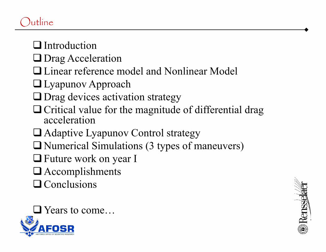
Numerical Simulations

� Simulations were performed using an STK scenario with High-Precision Orbit Propagator (HPOP) that included:

� Full gravitational field model

� Variable atmospheric density (using NRLMSISE-00)

� Solar pressure radiation effects

Obtain state

vector from

STK

Calculate Propagate in

Parameter Value

Target’s inclination (deg) 98

Target’s semi-major axis (km) 6778

Target’s right ascension of the

ascending node (deg)262

� Initial relative position of -1km in x, -2km in y in the LVLH

� The maneuver ended when S/C were within 10m.

Calculate

matrix

derivatives

Adapt

matrices Q,

and Ad

Run panel

activation

strategy

Propagate in

STK for 10

minutes Target’s argument of perigee (deg) 30

Target’s true anomaly (deg) 25

Target’s eccentricity 0

m(kg) 10

S(m2) 1.3

CD 2

Numerical Simulations (rendezvous)

�Simulated trajectory in the x-y plane

Numerical Simulations (rendezvous)

� Control signal for both controllers

NoAdaptation

With Adaptation

� aDcrit for both controllers� aDcrit for both controllers

� Adaptive VS Non Adaptive

� Number of control switches: 56 VS 113 (50% less actuation)

� Maneuver time: 29 hr VS 38 hr (24% less time)

Numerical Simulations (rendezvous)

� Error for both controllers

� Non adaptive Lyapunov controller needs more time and a higher control effort since itapproaches the rendezvous state performing larger oscillations

� The reduction on the maneuver time and the control effort is caused by the adaptation of thematrix P which allows the adaptive Lyapunov control to tune itself as the error evolves

Numerical Simulations (re-phasing)

1

1.5

2

2.5

y [

km

]

No Adaptation

Start

With Adaptation

0 0.1 0.2 0.3 0.4 0.5

-1

-0.5

0

0.5

1

Time [days]

Co

ntr

ol

Sig

na

l

-0.15 -0.1 -0.05 0 0.05-0.5

0

0.5

x [km]

0 0.1 0.2 0.3 0.4 0.5

-1

-0.5

0

0.5

1

Time [days]

Co

ntr

ol

Sig

na

l

Numerical Simulations (fly-around)

-2

-1.5

-1

-0.5

0

0.5

y [

km

]

No Adaptation

Start

With Adaptation

0 0.1 0.2 0.3 0.4

-1

-0.5

0

0.5

1

Time [days]

Co

ntr

ol

Sig

na

l

-0.4 -0.2 0 0.2 0.4-4.5

-4

-3.5

-3

-2.5

x [km]

y [

km

]

With Adaptation

Guidance

0 0.1 0.2 0.3 0.4

-1

-0.5

0

0.5

1

Time [days]

Co

ntr

ol

Sig

na

l

Future Work

�Include the linear reference model in the derivation

of:

�This will allow for tracking a desired path or the dynamics

of the linear reference model

,Dcrit Dcrita a∂ ∂∂ ∂

dA Q

�Further developments on the adaptation strategy are

expected to improve controller performance

�Attitude control via drag too(?)

Conclusions

� A novel adaptive Lyapunov controller for S/C autonomous rendezvous maneuvers using atmospheric differential drag is presented

� Analytical expressions aDcrit , are derived

� The quadratic Lyapunov function is modified in real time,

during flight using these derivatives, reducing a

,Dcrit Dcrita a∂ ∂∂ ∂

dA Q

during flight using these derivatives, reducing aDcrit

� Unprecedented ability to perform rendezvous to less than 10 meters without propellant

� Adaptive Lyapunov controller is an improvement

� Significantly lower control effort (50% less actuation)

� Less time to reach the desired rendezvous state (24% less time)

Accomplishments (April-September 2012)

Perez, D., Bevilacqua, R., "Differential Drag Spacecraft Rendezvous using an

Adaptive Lyapunov Control Strategy", accepted for publication on Acta

Astronautica, to appear.

BEST STUDENT PAPER AWARD FOR THE CATEGORY: SPACECRAFT

GUIDANCE, NAVIGATION, AND CONTROL.

1st International Academy of Astronautics Conference on Dynamics and Control

of Space Systems – DyCoSS’2012, Porto, Portugal, 19-21 March 2012.

BEST ORAL PRESENTATION in the Theoretical Category:

Undergraduate research by Skyler Kleinschmidt at the Rensselaer’s Third Annual

Undergraduate Research Symposium: “Origami-Based Drag Sail for Differential

Drag Controlled Satellites”, Wednesday, April 4, 2012.

Submitted NSF proposal using differential drag, in collaboration with NASA

scientist

Year II

� Study a new methodology to estimate drag and reconstruct

neutral density

� Repeat simulations using GRACE (Gravity Recovery and

Climate Experiment) data. This data was kindly provided at

AFRL Kirtland AFB, during AF SFFP (summer 2012)AFRL Kirtland AFB, during AF SFFP (summer 2012)

� Forecasting on given orbit possible?

Year III

� 2U Cubesat, hosting a deployable sail in 0.5U

� Clear mylar used for the sail (space qualified, and letting sun

get through)

� Sail design based on an origami folding pattern, to maximize

surface, and minimize volume when contracted

Questions