SOLUTION - Leica Microsystems TCS SP5 II... · Figure 3: Live Data Mode tool Monitor tab 1 2 7 6 3 5 4. ... (Fig. 3) contains the ... ment using sequential scan mode. When this option

reSOLUTION

CONFOCAL APPLICATION LETTER

D e c .

2 0 0 7

N o. 2 7

Live Data Mode with Leica TCS SP5

Content

1. How to get started . . . . . . . . . . . . . . . . . . . . . . . . . . . . . . . . . . . . . . . . . . 3

2. Interactive Data Acquisition . . . . . . . . . . . . . . . . . . . . . . . . . . . . . . . . . 5

3. Pre-Defi nition of Experiment Settings . . . . . . . . . . . . . . . . . . . . . . . . . 7

4. Setting Up an Experiment (Job Macro) . . . . . . . . . . . . . . . . . . . . . . . . 9

4.1 Combining Jobs in a Macro . . . . . . . . . . . . . . . . . . . . . . . . . . . . 10

4.2 Pause . . . . . . . . . . . . . . . . . . . . . . . . . . . . . . . . . . . . . . . . . . . . . . . 12

4.3 Loops . . . . . . . . . . . . . . . . . . . . . . . . . . . . . . . . . . . . . . . . . . . . . . . . 12

4.4 Trigger Settings . . . . . . . . . . . . . . . . . . . . . . . . . . . . . . . . . . . . . . 13

5. Data Handling . . . . . . . . . . . . . . . . . . . . . . . . . . . . . . . . . . . . . . . . . . . . . . 19

Titel Page:

Cell Type MDA MB-231. Time lapse: time points of acquisition each 20 min. Blue CD44- CFP (plasmatic membrane)

Red Vimentin-mRFP (Focal Adhesions). Green Actin -YFP (Cytoskeleton). Magenta Lamin A-GFP (Nuclear envelope)

Courtesy Dr. Maria Montoya, Confocal Microscopy and Cytometry Unit, CNIO, Madrid, Spain

Live Data Mode

3Confocal Application Letter

Live Data Mode in LAS AF

with Leica TCS SP5

Introduction

Live cell imaging applications comprise

many different kinds of specimen and

scientifi c interests including dynamic

studies, drug and cancer research, e.g.

interaction between immune cells in

cell cultures and following changes of

gene expression in developmental biol-

ogy in live embryos. All these applica-

tions require a fl exible instrument and

software that allows for online interac-

tion with hardware control settings in

order to improve experimental condi-

tions and prolong cell viability during

an experiment. For more advanced ap-

plications it is important to pre-defi ne

settings and confi gure time lapse se-

quences.

The Live Data Mode tool in LAS AF is

designed for live cell experiments and

dynamic investigations: the scientist

can defi ne an experiment before data

acquisition to carry out manipulations

on the living specimen, e.g. application

of a drug, switching of external devices

etc., or pausing the experiment which

is a prerequisite for good experimental

control.

Direct interaction with the instrument

is also highly important: this means

the possibility of changing hardware

parameters like laser power, scanning

speed, acquisition channels or other

imaging settings during the running ex-

periment.

1. How to get started

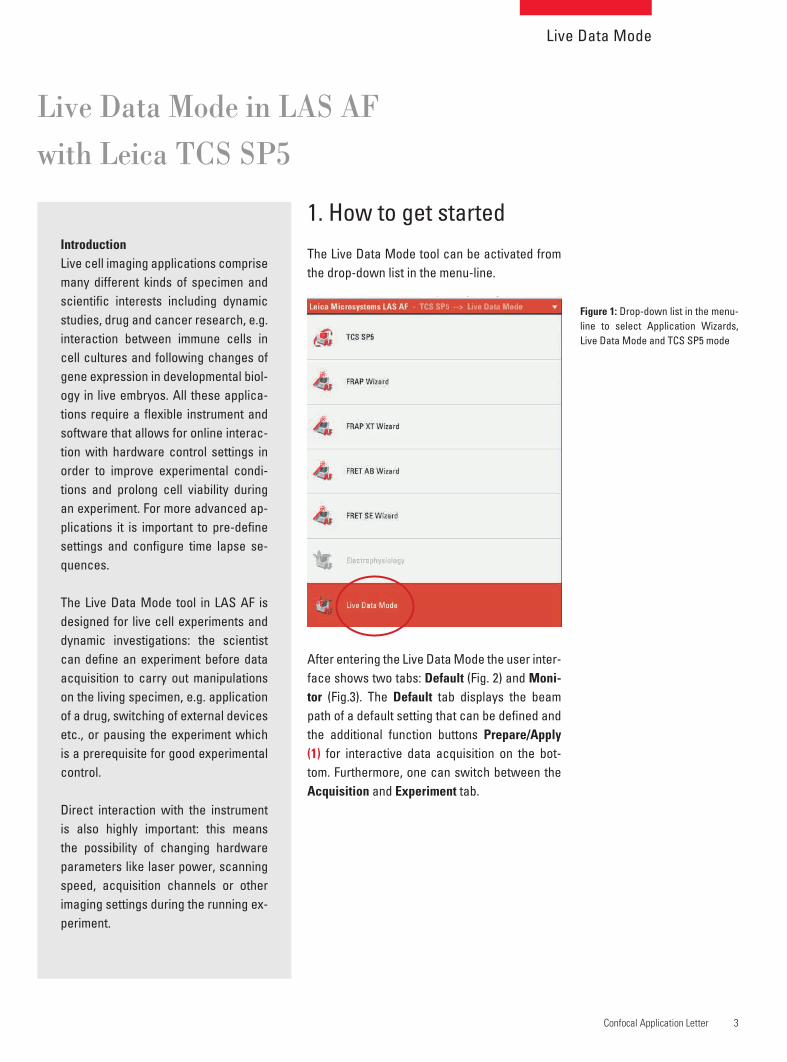
The Live Data Mode tool can be activated from

the drop-down list in the menu-line.

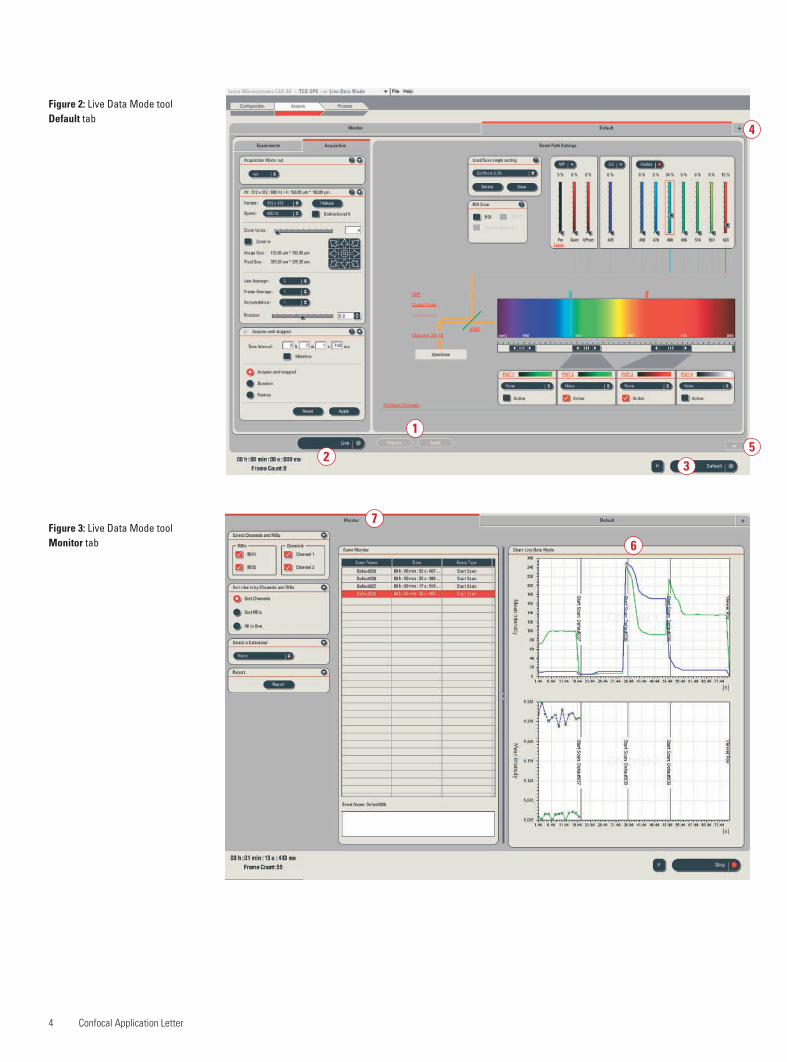
After entering the Live Data Mode the user inter-

face shows two tabs: Default (Fig. 2) and Moni-

tor (Fig.3). The Default tab displays the beam

path of a default setting that can be defi ned and

the additional function buttons Prepare/Apply

(1) for interactive data acquisition on the bot-

tom. Furthermore, one can switch between the

Acquisition and Experiment tab.

Figure 1: Drop-down list in the menu-

line to select Application Wizards,

Live Data Mode and TCS SP5 mode

4 Confocal Application Letter

Figure 2: Live Data Mode tool

Default tab

Figure 3: Live Data Mode tool

Monitor tab

1

2

7

6

3

5

4

Live Data Mode


Live Scan

Before starting an experiment the adjustment

of imaging conditions can be carried out during

Live-Scan (2). No experiment fi le is generated in

this case.

Default

This function defi nes the hardware control set-

tings for an experiment or a part of an experi-

ment. Available scan modes are: xt, xyt and xyzt.

The execution of the Default setting (3) automat-

ically generates an experiment folder named

“LDM” which contains a fi le named “Default

001” (see also section Data Handling, page 19).

Experiment sequences (jobs) can be added by

using the plus symbol (4) and be deleted by us-

ing the minus-symbol (5).

Note: The default setting can be freely changed

but not be deleted.

Online Quantifi cation

Online quantifi cation of several regions of inter-

est (ROIs) is crucial for live cell imaging applica-

tion. Especially for the monitoring of changes in

fl uorescence intensity during the running exper-

iment it is benefi cial to see images in the viewer

and quantifi cation charts simultaneously.

The Monitor tab (Fig. 3) contains the quantifi ca-

tion tool with the graph display (Chart) (6) for on-

line measurements as well as the Event Monitor

list (7).

Subsequently, the mean intensity of each ROI

is displayed online within the Chart (right). The

ROIs can be moved during image acquisition.

The Event Monitor list (middle) shows the time

point and type of events, e.g. switching of jobs

and triggers.

2. Interactive Data Acquisition

For optimal adaptation of the imaging conditions

to the specimen and the experiment, the Live

Data Mode tool allows for directly interaction

with the hardware control settings so that imag-

ing parameters can be easily optimized during

the running experiment.

Interactive changes of hardware settings

During the running experiment (default setting

or any added job) the current hardware settings

can be changed interactively by clicking on

Prepare (1) (Fig. 4a). The user interface is now

situated in a virtual mode and gives access to all

imaging parameters (2) that can be changed and

optimized (see also box page 6).

By clicking on Apply (3) the new settings are ap-

plied to the further imaging. Now the system is

ready again for new hardware changes.

After each change of the hardware settings by

using the Prepare/Apply function the system

starts scanning a new series that appears un-

der Experiments as a data fi le in the LDM folder.

These changes are indicated in the event list

and graph within the Monitor tab.

In order to apply certain hardware settings (job)

on demand during a running default-setting a

new setting (job) needs to be added and defi ned

(see section Pre-Defi nition of Experiment Set-

tings, page 7).

Note: When the job is completed the system

switches automatically to scan using the De-

fault setting.


Parameters for imaging that can

be changed interactively by using the

Prepare/Apply function:

• scan mode

• scan format and speed

• line and frame average

• accumulation

• changes in the t-dialog (minimize

= minimized time interval between

each frame, defi nition of time

duration or number of frames)

• changes in the z-dialog

• adding/reducing number of PMTs

• switching of additional channels

(PMT Trans or NDDs)

• changing of control panel confi gura-

tion

Parameters that can be changed online

without use of Prepare/Apply function:

• PMT gain and offset

• laser power by AOTF

• adding/removing of laser lines

• zoom factor

• scan fi eld rotation

• pinhole size

• AOBS settings

Pausing data acquisition interactively

The manipulation of living specimen sometimes

requires pausing of the data acquisition during a

running experiment. For example cells are moni-

tored without any treatment; the data acquisition

is paused while a drug is applied. Subsequently,

the data acquisition is continued for the moni-

toring of cell reactions. Pausing of scanning can

be done interactively at any time just by a click

on the Pause button (4) located bottom right (Fig.

4b). To continue data acquisition the Pause but-

ton needs to be clicked again.

Figure 4a: Activated Prepare

function: hardware settings can be

accessed in the Acquisition tab

1 3

2

Live Data Mode


Figure 4b: System is ready for the

next interactive hardware change:

Prepare needs to be pressed again

to access hardware settings

3. Pre-Defi nition of Experiment Settings

Beside interactive data acquisition the pre-

defi nition of individual experimental job settings

within time lapses is relevant. With the pre-def-

inition any experimental setting can be used for

a certain time. Also the time course of advanced

applications can be pre-defi ned, saved and re-

used again for reproducible experiments. The

Live Data Mode tool enables the scientist to

easily confi gure these kinds of experiments by

defi ning jobs and job macros.

Adding Jobs

A Job can be added by clicking on the plus sym-

bol (1) top right in the beam path window (Fig.

5a). Three options are available from a list (2)

(Fig. 5b):

1. Job: a standard time lapse experiment with-

out sequential scan mode.

2. Job (Sequential Scan): a time lapse experi-

ment using sequential scan mode. When this

option is selected the sequential scan dialog

appears automatically in the Acquisition tab on

the left side.

3. Macro: a tool for confi guring Jobs in a certain

order, defi nition of pauses and loops between

Jobs, assignment of triggers to jobs, access to

trigger settings dialog.

Figure 5a: Plus symbol for adding a job

Figure 5b: Options for adding a job

1

2

4


Figure 6: Specifi c settings of Job1 (6a) and Job2 (6b)

6a Specifi c settings of Job1:

5 frames, 488 nm ex, detection

window 505-568 nm, PMT 2

6b Specifi c settings of Job2:

time interval minimized, 20

frames, 633 nm ex, detection

window 635-700 nm, PMT 3

3

4

Live Data Mode


Defi ning Job Settings

After adding the fi rst job, the hardware settings

can be defi ned independently from the default

settings. For each job added the beam path and

the settings appear in an individual tab. Thus, by

selecting the Job tab the settings for each job

can be viewed, controlled and modifi ed if nec-

essary (see Fig. 6a and 6b).

The system automatically counts the added jobs

(Job 1, Job 2, Job 3 etc.).

If several jobs are to be defi ned a newly added

job will contain the same settings as the job that

was selected during the addition, e.g. if the tab

of Job 1 is selected the settings of Job 1 are

automatically applied to the new job (Job 2).

Jobs can be started with a click on the appropri-

ate Start button (3) (Fig. 6a) which appears bot-

tom right below the beam path window. During a

running job or default setting interactive chang-

es of imaging parameters can be performed as

described earlier in section Interactive Data Ac-

quisition, page 5.

Deleting, Renaming and Saving Jobs

A job can be deleted by clicking on the Job tab

and a subsequent click on the minus symbol (4)

(Fig. 6b). The system continues its way of count-

ing jobs no matter if a previous job has mean-

while been deleted. So, if an old Job (Job 3)

was deleted and another job is added it will be

named Job 4.

Deleting, renaming and saving jobs can also be

done with a right mouse click on the Job tab.

(Fig. 7).

Figure 7: Options for job handling

4. Setting Up an Experiment (Job Macro)

Many applications require a good experimental

defi nition within time lapses. For example, when

the effect of a drug is studied on living cells the

experiment may be defi ned as follows:

Job 1 Cells are observed without any treatment

for a certain time.

Job 2 After the application of the drug the cells

react and the organelles move much

faster. Now, imaging parameters can

be adapted accordingly by pre-defi ning

short time intervals for data acquisition

for a certain time.

Job 3 After 5 min the cells react slowly and

data acquisition can be performed with

longer time intervals.

In developmental biology the acquisition speed

can be adapted to the investigated processes,

e.g. the movements of cells within the embryo or

cell division. This is done by defi ning jobs with

different settings for the time interval.

The Live Data Mode provides many possibilities

to defi ne advanced time lapses by free con-

fi guration of jobs and their combination in a job

macro. The key features of the job macro are

listed on page 10.


4.1 Combining Jobs in a Macro

To defi ne an experiment macro the option Mac-

ro must be selected after clicking on the plus

symbol (Fig. 8).

Then a new tab named Job Macro 1 is generat-

ed (Fig. 9a and b). All previous defi ned Jobs are

listed on the top left (1). For Job and Macro han-

dling the functions Add, Insert, Remove, Load,

Save Macro are available (2). In a job macro

Trigger Settings, Loop and Pause (3) can be se-

lected. By a click on a job and subsequently on

Add, the job is transferred into the grey time line

below (4) (Fig 9b).

Job Macro Key Features

1. Combining different jobs to design a job macro: pre-defi nition of experiments consisting

of several jobs

2. Pause of data acquisition at a certain time point for a defi ned duration of time

3. Loops: repeated data acquisition using certain imaging parameters that includes loop-

ing of one job or a part of an experiment

4. Triggering: synchronizing the scanning process with external devices

Figure 8: Options for adding

Figure 9a: User interface of

Job Macro 1 with listed Jobs

and time line

Figure 9b: Jobs have been added

into the time line (Job Macro 1)

1 2 3

4

Live Data Mode

A job can be removed from the time line by a

click on the particular job in the time line and a

subsequent click on Remove (8). Jobs that have

been removed from the time line are still avail-

able as a Job tab.

Save and reload of a job macro

In order to get reproducible experiments a job

macro can be saved and reloaded by the two

function buttons Save Macro (10) and Load (9)

(Fig. 9c). The macro will be saved under a default

name given by the software, e.g. Job Macro 2.

It can be renamed afterwards.

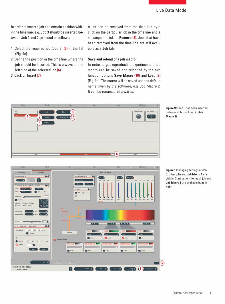
In order to insert a job at a certain position with-

in the time line, e.g. Job 3 should be inserted be-

tween Job 1 and 2, proceed as follows:

1. Select the required job (Job 3) (5) in the list

(Fig. 9c).

2. Defi ne the position in the time line where the

job should be inserted. This is always on the

left side of the selected job (6).

3. Click on Insert (7).


Figure 9c: Job 3 has been inserted

between Job 1 und Job 2 (Job

Macro 1)

Figure 10: Imaging settings of Job

3. Other jobs and Job Macro 1 are

visible. Start buttons for each job and

Job Macro 1 are available bottom

right

12

11

5 7

9

8

6

10


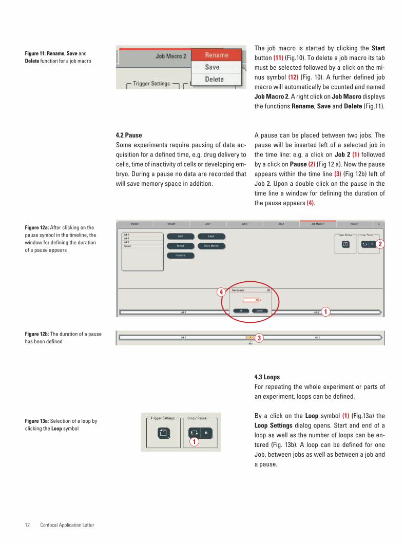
4.3 Loops

For repeating the whole experiment or parts of

an experiment, loops can be defi ned.

By a click on the Loop symbol (1) (Fig.13a) the

Loop Settings dialog opens. Start and end of a

loop as well as the number of loops can be en-

tered (Fig. 13b). A loop can be defi ned for one

Job, between jobs as well as between a job and

a pause.

The job macro is started by clicking the Start

button (11) (Fig.10). To delete a job macro its tab

must be selected followed by a click on the mi-

nus symbol (12) (Fig. 10). A further defi ned job

macro will automatically be counted and named

Job Macro 2. A right click on Job Macro displays

the functions Rename, Save and Delete (Fig.11).

4.2 Pause

Some experiments require pausing of data ac-

quisition for a defi ned time, e.g. drug delivery to

cells, time of inactivity of cells or developing em-

bryo. During a pause no data are recorded that

will save memory space in addition.

Figure 11: Rename, Save and

Delete function for a job macro

Figure 12a: After clicking on the

pause symbol in the timeline, the

window for defi ning the duration

of a pause appears

Figure 12b: The duration of a pause

has been defi ned

Figure 13a: Selection of a loop by

clicking the Loop symbol

A pause can be placed between two jobs. The

pause will be inserted left of a selected job in

the time line: e.g. a click on Job 2 (1) followed

by a click on Pause (2) (Fig 12 a). Now the pause

appears within the time line (3) (Fig 12b) left of

Job 2. Upon a double click on the pause in the

time line a window for defi ning the duration of

the pause appears (4).

1

4

1

2

3

Live Data Mode

Figure 13c: Selection of a loop for deletion

A click on Defi ne Loop (2) applies the Loop to the

experiment Macro in the time line (Fig. 14). For

removing a loop it has to be selected in the list


Figure 14: A loop is indicated in the

job macro

Figure 13b: The Loop Settings dialog has opened and a loop

can be defi ned

Figure 15: A click on Trigger Settings

opens the Trigger Settings dialog

1

2

3

4

of existing loops (3) followed by a click on the

button Remove Loop (4) (Fig. 13c).

4.4 Trigger Settings

To synchronize the scanning process with ex-

ternal devices (patch pipettes, electrodes etc.)

trigger functions can be used. For these ap-

plications it is a prerequisite that the system is

equipped with the Leica trigger unit.

All defi ned triggers are recorded automatically

in the event monitor list and are indicated by a

marker within the graph. Therefore, in the trigger

settings dialog checking is not necessary in Re-

cord in Event List and Show in Graph.

To assign a trigger to an individual job this job

must fi rst be selected in the time line. A subse-

quent click on the Trigger symbol (1) (Fig. 15)

opens the Trigger Settings dialog that allows

for setting input (IN) and output triggers (OUT)

(Fig. 16).

3 4 5

2

6

7

2

Trigger IN

Using a signal from an external device (patch

clamp system, micromanipulator) for triggering

the start of scanning, two free confi gurable in-

put triggers are available.The scan starts when

the trigger signal arrives in the scan head. When

the system is equipped with an extension for

FCS only one input trigger is available for the

Live Data Mode tool as one input trigger is con-

fi gured for the FCS-application.

Note: A certain time is required to position the

y-galvo for scanning a frame: this time duration

needed from the beginning of a trigger-pulse to

(3) Trigger IN on Frames

Input triggers can be defi ned at begin of a job in

the xyt-scan mode.

Note: The functions First Trigger at and Repeat

every are currently not working for input trig-

gers.

the scan start (Delta T) depends on the scan

speed and format (see Fig. 19). In addition to the

Delta T, a little time is required to position the

x-galvo. The maximum time needed is equal to

the time needed to scan one line (for 1000 Hz =

1ms). However, input triggers react reproduc-

ible. Without considering the time needed for

positioning the x-galvo reproducability is within

10 µsec.

To assign an input trigger to a job the appropri-

ate trigger channel has to be selected from the

drop down list (2) (Fig.16) .

Figure 16: Trigger settings

Confocal Application Letter14

Application:

1. Upon the action of a patch-

pipette its signal is used to

trigger the start of a job.

2. If a hand-held pipette deliv-

ers the drug to the speci-

men the Trigger In signal

can be used to start the

data acquisition (hand- or

footswitch).

txyt-frames

JobBegin End

Scanner

Trigger in

External device

Trigger OUT

To start the action of an external device on a de-

fi ned time point four freely confi gurable output

triggers are available (Fig. 16). In this case the

trigger signal is send from the scan head to the

external device (e.g. a patch clamp system) to

start its operation.

To assign an output trigger to a job the appropri-

ate trigger channel from the drop down list (2)

has to be selected (Fig.16). The defi ned trigger

is indicated in the time line (Fig. 17).

(4) Trigger OUT on function Start:

An output trigger can be set at the beginning of

the fi rst frame of a job or at the beginning of a

pause.

Live Data Mode


(5) Trigger OUT on function End:

An output trigger can be defi ned at the end of

the last frame of a job or at the end of a pause.

(Red arrows indicate trigger pulses)

Figure 17: Job macro with activated

out-trigger (OUT1) at the begin of Job 2

Applications:

1. Microinjection to manipulate the specimen at a defi ned time point: a microinjection pi-

pette is attached to the incubation medium. Scanning is performed to acquire control data

in Job 1. The Trigger Out signal from the scanner can be used to start the injection at a

defi ned time point within the experiment. Thus, at the beginning of Job 2 an output trigger

starts the action of a micropipette that delivers a drug to a cell preparation.

2. Adding a certain buffer to the medium at the begin or the end of a job.

Output triggers can be defi ned at the begin and the

end of a job or pause as indicated below.

Note: The reaction time for output triggers on

function start (4) and output triggers on function

end (5) can not be predicted like the input trig-

gers because they are realized by software.

xyt-frames

Job/PauseBegin

t

End

Scanner

Trigger out

External device

xyt-frames

Job/PauseBegin

t

End

Scanner

Trigger out

External device


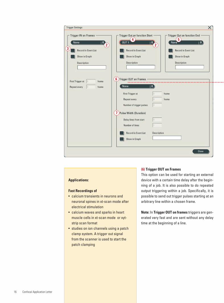
(6) Trigger OUT on Frames

This option can be used for starting an external

device with a certain time delay after the begin-

ning of a job. It is also possible to do repeated

output triggering within a job. Specifi cally, it is

possible to send out trigger pulses starting at an

arbitrary line within a chosen frame.

Note: In Trigger OUT on frames triggers are gen-

erated very fast and are sent without any delay

time at the beginning of a line.

3

4 5

6

7

2 2

Applications:

Fast Recordings of

• calcium transients in neurons and

neuronal spines in xt-scan mode after

electrical stimulation

• calcium waves and sparks in heart

muscle cells in xt-scan mode or xyt-

strip scan format

• studies on ion channels using a patch

clamp system. A trigger out signal

from the scanner is used to start the

patch clamping

Live Data Mode


xyt-scan mode

For setting a delay a number needs to be entered

in First Trigger at … frame.

The sending of an output trigger in xyt-scan

mode can be repeated within a Job. Repeat-

ing frequency has to be set in Repeat every …

frame. If a certain number of triggers should be

send starting on a certain frame a number needs

to be entered in number of trigger pulses.

xt-scan mode

A delayed trigger pulse is set at the beginning

of a certain xt-page (see left). Here the term

“page” corresponds to frame.

Repeated output triggering in xt-scan mode

requires the defi nition of several pages within

the time-dialog in the Acquisition tab. For fast

repeats it is recommended to defi ne a small

number of lines per page, e.g. below 1000. The

maximum number of lines per page is 8192.

(Red arrows indicate trigger pulses)xt-pages

xyt-frames

JobBegin

t

End

Scanner

Trigger out

External device

xt-pages

JobBegin

t

End

Scanner

Trigger out

External device

xyt-frames

JobBegin

t

End

Scanner

Trigger out

External device


(7) Pulse-Position and Width for XT-Scan Mode

A delayed output trigger from the start of a page

can be defi ned by counting lines from start. The

delay needs to be defi ned in Delay lines from

start (Fig.16). The duration of a trigger pulse can

be set in Number of lines (see also Fig. 18).

Figure 18: Setting trigger pulse du-

ration and position (delay) in xt-scan

mode by defi ning lines: This example

shows a position of the trigger pulse

four lines after the page start. The

trigger pulse lasts for another six

lines.

Figure 19a: Scheme on Delta T

Image

Trigger

Delta T

t

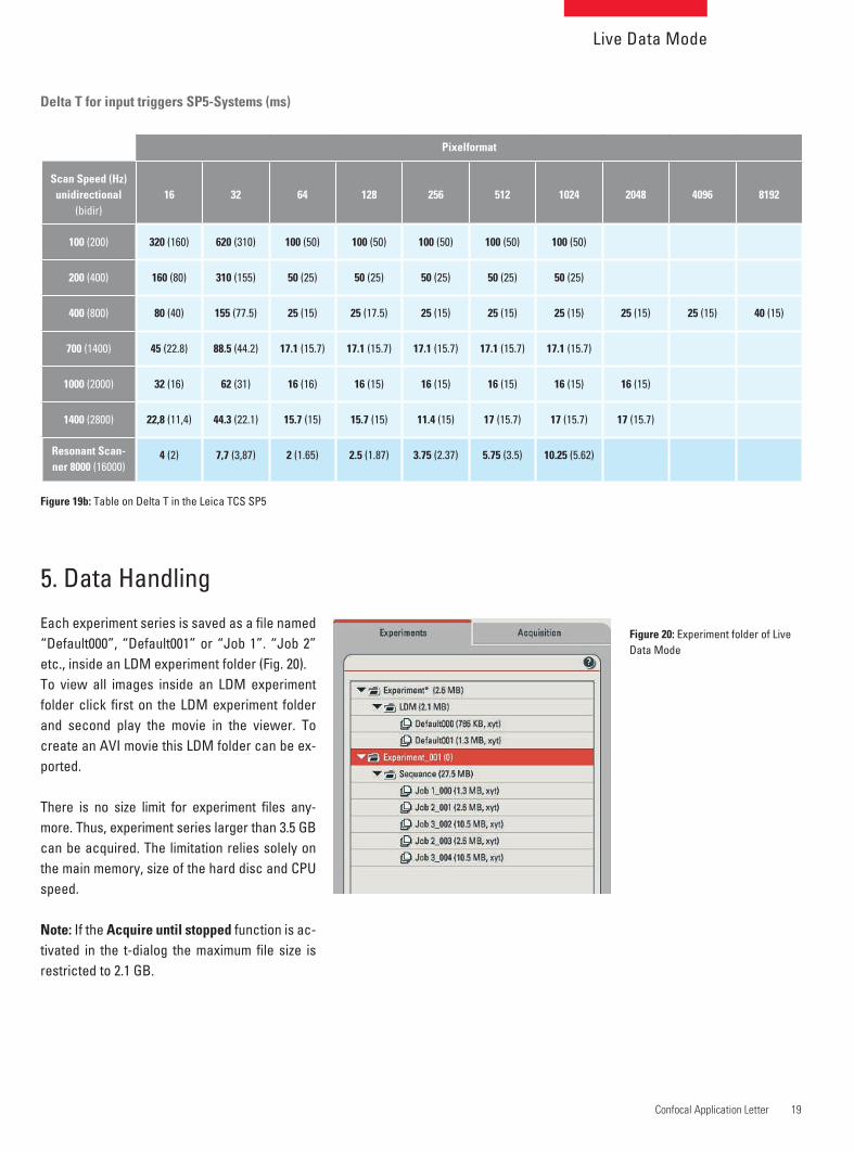
Trigger Timing (Delta T) for Input Triggers

The time from begin of a trigger pulse to the

scan of the 1st image pixel (Delta T) depends on

the scan speed. See scheme and data regarding

timing (Fig 19a and 19b).

lines trigger pulse position (delay)

pages

4 lines

trigger pulse

duration:

6 lines

t

1

2

3

4

5

6

7

8

9

10

11

12

13

14

15

16

Live Data Mode


Delta T for input triggers SP5-Systems (ms)

Figure 19b: Table on Delta T in the Leica TCS SP5

Figure 20: Experiment folder of Live

Data Mode

Pixelformat

Scan Speed (Hz)

unidirectional

(bidir)

16 32 64 128 256 512 1024 2048 4096 8192

100 (200) 320 (160) 620 (310) 100 (50) 100 (50) 100 (50) 100 (50) 100 (50)

200 (400) 160 (80) 310 (155) 50 (25) 50 (25) 50 (25) 50 (25) 50 (25)

400 (800) 80 (40) 155 (77.5) 25 (15) 25 (17.5) 25 (15) 25 (15) 25 (15) 25 (15) 25 (15) 40 (15)

700 (1400) 45 (22.8) 88.5 (44.2) 17.1 (15.7) 17.1 (15.7) 17.1 (15.7) 17.1 (15.7) 17.1 (15.7)

1000 (2000) 32 (16) 62 (31) 16 (16) 16 (15) 16 (15) 16 (15) 16 (15) 16 (15)

1400 (2800) 22,8 (11,4) 44.3 (22.1) 15.7 (15) 15.7 (15) 11.4 (15) 17 (15.7) 17 (15.7) 17 (15.7)

Resonant Scan-

ner 8000 (16000)4 (2) 7,7 (3,87) 2 (1.65) 2.5 (1.87) 3.75 (2.37) 5.75 (3.5) 10.25 (5.62)

5. Data Handling

Each experiment series is saved as a fi le named

“Default000”, “Default001” or “Job 1”. “Job 2”

etc., inside an LDM experiment folder (Fig. 20).

To view all images inside an LDM experiment

folder click fi rst on the LDM experiment folder

and second play the movie in the viewer. To

create an AVI movie this LDM folder can be ex-

ported.

There is no size limit for experiment fi les any-

more. Thus, experiment series larger than 3.5 GB

can be acquired. The limitation relies solely on

the main memory, size of the hard disc and CPU

speed.

Note: If the Acquire until stopped function is ac-

tivated in the t-dialog the maximum fi le size is

restricted to 2.1 GB.

Leica Microsystems –

the brand for outstanding productsLeica Microsystems’ mission is to be the world’s first-choice provider of innovative solutions to our

customers’ needs for vision, measurement and analysis of micro-structures.

Leica, the leading brand for microscopes and scientific instruments, developed from five brand

names, all with a long tradition: Wild, Leitz, Reichert, Jung and Cambridge Instruments. Yet Leica

symbolizes innovation as well as tradition.

Leica Microsystems – an international company

with a strong network of customer services

Australia: North Ryde Tel. +61 2 8870 3500 Fax +61 2 9878 1055

Austria: Vienna Tel. +43 1 486 80 50 0 Fax +43 1 486 80 50 30

Belgium: Groot Bijgaarden Tel. +32 2 790 98 50 Fax +32 2 790 98 68

Canada: Richmond Hill/Ontario Tel. +1 905 762 2000 Fax +1 905 762 8937

Denmark: Herlev Tel. +45 4454 0101 Fax +45 4454 0111

France: Rueil-Malmaison Tel. +33 1 47 32 85 85 Fax +33 1 47 32 85 86

Germany: Wetzlar Tel. +49 64 41 29 40 00 Fax +49 64 41 29 41 55

Italy: Milan Tel. +39 02 574 861 Fax +39 02 574 03392

Japan: Tokyo Tel. + 81 3 5421 2800 Fax +81 3 5421 2896

Korea: Seoul Tel. +82 2 514 65 43 Fax +82 2 514 65 48

Netherlands: Rijswijk Tel. +31 70 4132 100 Fax +31 70 4132 109

People’s Rep. of China: Hong Kong Tel. +852 2564 6699 Fax +852 2564 4163

Portugal: Lisbon Tel. +351 21 388 9112 Fax +351 21 385 4668

Singapore Tel. +65 6779 7823 Fax +65 6773 0628

Spain: Barcelona Tel. +34 93 494 95 30 Fax +34 93 494 95 32

Sweden: Kista Tel. +46 8 625 45 45 Fax +46 8 625 45 10

Switzerland: Heerbrugg Tel. +41 71 726 34 34 Fax +41 71 726 34 44

United Kingdom: Milton Keynes Tel. +44 1908 246 246 Fax +44 1908 609 992

USA: Bannockburn/lllinois Tel. +1 847 405 0123 Fax +1 847 405 0164

and representatives of Leica Microsystems

in more than 100 countries.

Leica Microsystems operates internationally in four divi-

sions, where we rank with the market leaders.

• Life Science Research DivisionLeica Microsystems’ Life Science Research Division sup-

ports the imaging needs of the scientific community with

advanced innovation and technical expertise for the visu-

alization, measurement and analysis of microstructures.

Our strong focus on understanding scientific applications

puts Leica Microsystems’ customers at the leading edge

of science.

• Industry DivisionThe Leica Microsystems Industry Division’s focus is to

support customers’ pursuit of the highest quality end

result by providing the best and most innovative imaging

systems for their needs to see, measure and analyze the

microstructures in routine and research industrial appli-

cations, in materials science and quality control, in foren-

sic science investigations, and educational applications.

• Biosystems DivisionThe Biosystems Division of Leica Microsystems brings

histopathology labs and researchers the highest-quality,

most comprehensive product range. From patient to

pathologist, the range includes the ideal product for each

histology step and high-productivity workflow solutions

for the entire lab. With complete histology systems fea-

turing innovative automation and Novocastra™ reagents,

the Biosystems Division creates better patient care through

rapid turnaround, diagnostic confidence and close cus-

tomer collaboration.

• Surgical DivisionThe Leica Microsystems Surgical Division’s focus is to

partner with and support micro-surgeons and their care

of patients with the highest-quality, most innovative surgi-

cal microscope technology today and into the future.

www.leica-microsystems.com

Ord

er

no

. 15

9310

4014

· L

EIC

A a

nd

th

e L

eic

a L

og

o a

re r

eg

iste

red

tra

de

ma

rks

of

Leic

a I

R G

mb

H

Documents

SOLUTION - Leica Microsystems TCS SP5 II... · Figure 3: Live Data Mode tool Monitor tab 1 2 7 6 3 5 4. ... (Fig. 3) contains the ... ment using sequential scan mode. When this option