Solid-State NMR Studies of Biomolecular Motion

Solid-State NMR Studies of Biomolecular Motion:

Theory, Analysis, Pulse Sequences, and Phase Cycling

4th Winter School on Biomolecular Solid-State NMR, Stowe, VT, Jan. 10-15, 2016

Mei Hong

Department of Chemistry, MIT

Molecular Motion is Abundant in Biomolecules & is Important for Function

•  Ligand binding

•  Ion conduction

•  Protein folding

•  Enzyme catalysis

2

3

Local motions Global motions

•  Methyl & amine rotation (3-site jump)

•  Aromatic 180˚ ring flip

•  Small-amplitude torsional fluctuation •  e.g. Trp & His rings •  backbone amides

•  Sidechain rotameric jumps (e.g. Leu mt/tp)

•  trans-gauche isomerization

•  Large-amplitude motions of flexible loops & termini

•  Rigid-body uniaxial rotation of membrane proteins in lipid bilayers

•  Near-isotropic diffusion

•  Correlated motions of protein domains

Common Protein Motions in the Solid State

•  Timescales & amplitudes of motion from NMR •  Fast motion: sum tensor analysis

•  Experiments for measuring fast motion

•  Order tensors & order parameters •  Slow motion: difference tensor analysis

•  Experiments for measuring slow motion

Molecular motions can: •  average NMR lineshapes; •  reduce or enhance signal intensities; •  affect relaxation properties; •  complicate quantification; •  allow spectral editing (CP vs. DP)

Effects of Motion on Solid-State NMR Spectra

4

Rates & Amplitudes of Reorientational Motions

•  For stochastic motions, correlation function describes how long it takes

to randomize the molecular orientation. The characteristic decay time is τc;

•  Rates: k (s-1) is inversely related to correlation time τc. Rate (s-1) ≠ frequency (Hz).

C t( ) ~ f 0( ) ⋅ f t( )

•  Amplitudes: denotes reorientational angle βR and the number of sites nR.

•  We do not consider translational motion here, since it is typically studied by pulsed-field-gradient NMR.

•  Diffusive motion: infinitesimal βR, infinite nR, e.g. isotropic tumbling, uniaxial diffusion, torsional fluctuation or libration.

•  Discrete (jump) motion: finite βR, finite nR; e.g. Methyl 3-site jump: for the C-H bond, βR = 109.5˚, nR = 3.

•  Phenylene ring flip: for the ortho/meta C-H bond, βR = 120˚, nR = 2.

τc

5

6

Motional Regimes Accessible From NMR

•  Fast motion: k >> Δω or δ, typically τc < 1 µs •  Amplitudes: obtained from spectral line narrowing;

•  Expts: DIPSHIFT, LG-CP, WISE, CSA narrowing, 2H spectra, etc. •  Rates: > 10 x δ; Exact rate requires relaxation NMR;

•  Slow motion: k << Δω, typically τc > 1 ms •  Measured by exchange NMR experiments (both static and MAS); •  Amplitudes: from 2D cross peaks, Ntr-dependent CODEX intensities. •  Rates: measured as the decay constant in tm-dependent intensities; •  # of sites: from the final value of the CODEX mixing-time curve.

•  Intermediate motion: k ~ Δω. •  Manifests as intensity loss, due to interference with 1H decoupling & MAS; •  Rates: from T2 and T1ρ minima in log(T2,1ρ) plots against 1/T. •  Amplitudes: from asymmetric DIPSHIFT intensity decays

Effects of Motion on NMR Lineshapes

Palmer, Chem. Rev. 2004.

Intermediate motion: k ≈ ωA −ωB

equal population (pA = pB = 0.5)

skewed population (pA = 0.75; pB = 0.25)

Slow motion: k << ωA −ωB

Measured during a mixing time.

Fast motion: k >> ωA −ωB

Average frequencies, can be calculated given a motional model.

ω

7

SSNMR Studies of Molecular Dynamics

8





ω = pjω jj

∑

• Σ has 3 principal axes (Σ1, Σ2, Σ3).

• Σ is characterized by δ, η, which reflect the geometry of motion.

• B0 orientation with Σ: (θa, φa ).

Motional Averaging of NMR Frequencies

ω θ ,φ( ) = 12δ 3cos2θ −1−η sin2θ cos2φ( )

Reorientation among N sites with probability pj gives an averaged tensor:

• In general, δ ≠δ, η ≠η.

• For dipolar couplings, δ can be sign- sensitive, and η ≠ 0.

ω θa ,φa( ) =δ 12 3cos2θa −1−η sin2θa cos2φa( )

Once the average tensor is known, we can predict the motionally averaged spectrum.

average tensor: Σ = pjσ jj

∑

For a tensor σ :

How do we determine δ and η? 9

10

Motionally Averaged δ and η

•  For uniaxial rotation and N ≥ 3 CN jumps, the z-axis of the sum tensor is the symmetry axis, zD.

•  is the frequency when B0 is parallel to the z-axis of the Σ tensor, where motion does not change the B0 orientation with the original PAS, thus the frequency is ω(θPD, φPD).

δ

From symmetry: •  Isotropic motion:

•  Uniaxial rotation:

•  N ≥ 3 CN jumps: η = 0

If a distribution of θPD:

δ = 0

}

δ =ω θPD ,φPD( )= 1

2δ 3cos2θPD −1−η sin2θPD cos2φPD( )

11

Methyl 3-Site Jumps

Palmer, Williams, and McDermott, J. Phys. Chem., 100, 13293 (1996).

2H spectra of C-H bond

slow intermediate fast

k 104 s-1 106 s-1 108 s-1

• C-H (η = 0, θPD =109.5˚): δ = 1

2δ 3cos2 109.5°−1( ) =−δ 3, η = 0

Order parameter : S ≡δ δSCH ,methyl = −1 3

SHH ,methyl = −1 2

"#$

%$

• H-H (η = 0, θPD = 90˚): δ = 1

2δ 3cos2 90°−1( ) =−δ 2, η = 0

δ =ω θPD ,φPD( ) = 12δ 3cos2θPD −1−η sin2θPD cos2φPD( )

12

Sum Tensor for Two-Site Jumps

ωn =1

2δ 3cos2Θn −1( )

The Σ tensor is invariant under A-B switching:

So the 3 principal axes should be:

The principal values of the averaged tensor:

σA σB

Σ1 axis: β/2, β/2 Σ2 axis: 90˚+β/2, 90˚-β/2 Σ3 axis: 90˚, 90˚

i 1, 2, 3 convention: left to right, i.e. ω1 >ω2 >ω3

i β < 90˚ and β > 90˚ switch Σ1 & Σ2 axes.

Σ3: Normal to the AOB plane Σ1: Bisector of the AOB angle Σ2: Normal to the bisector in the AOB plane

Σ = σ A +σ B( ) 2 = σ B +σ A( ) 2

Θn: angles between zPAS and Σn

For 2-site jumps averaging a uniaxial (η = 0) tensor, we can figure out the Σ tensor principal values using the same approach: calculate the frequency when B0 is parallel to a principal axis of the Σ tensor.

Θ1 = 30°

Θ2 = 60°

Θ3 = 90°

"

#$

%$

⇒

ω1 = 58δ

ω2 = − 18δ

ω3 = − 12δ

"

#$$

%$$

⇒δ = 5

8δ

η=0.6

"

#$

%$

13

Two-Site Jumps: Phenylene Ring Flip Consider 2H or C-H dipolar spectra (η = 0): Reorientation angle βR = 120˚.

η ≠ 0 for the average dipolar tensor.

ωn =1

2δ 3cos2Θn −1( )

14

Two-Site Jumps: trans-gauche Isomerization

Palmer, Williams, and McDermott, J. Phys. Chem., 100, 13293 (1996).

2H spectra

slow intermediate fast

k 104 s-1 106 s-1 108 s-1

δ =12δ, η =1

βR = 109.5˚: Θn = 35.3˚, 54.7˚, 90˚: ⇒ ωn =

δ2

, 0, −δ2

.

For C-H dipolar coupling or 2H quadrupolar coupling:

Two-Site Jumps: Histidine 180˚ Ring Flip

ωn = 12δ 3cos2Θn −1( )

180˚ jump around the Cβ-Cγ bond (χ2 change):

βR = 2 ⋅57˚=114˚For the Cγ-Nδ1 bond:

Θ1 = 33°

Θ2 = 57°

Θ3 = 90°

"

#$

%$

⇒ω1 = 0.56δ

ω2 = −0.06δ

ω3 = −0.5δ

"

#$

%$

⇒δ = 0.56δ

η = 0.79

"#$

%$⇒ SCγ−Nδ1 = 0.56

For the Cδ2-Hδ2 bond: βR =156˚ ⇒ δ = 0.94δ ⇒ SCδ2−Hδ2 = 0.9415


16





v  Active recoupling of X-1H dipolar coupling

§  T-MREV

§  15N-1H REDOR in deuterated proteins with back exchanged 1H

§  Symmetry-based R sequences, ~<40 kHz

17

X-1H Dipolar-Shift Correlation (DIPSHIFT) v  Passive sampling of X-1H dipolar coupling in a rotor period combined with

active 1H-1H decoupling §  MREV-8: ≤ 7 kHz §  LG-CP: < 20 kHz §  FSLG, PMLG, eDUMBO: ~< 40 kHz

e.g. R1431 , R163

2, R1841 , R265

3, R2854

ω1 /ωr 2.33 2.67 2.25 2.6 2.8

k 0.27 0.28 0.26 0.27 0.28

Polenova et al.

Schanda, Meier, Ernst et al.

18

•  A separated-local-field (SLF) technique (≠ PDLF, LG-CP, or PISEMA).

•  1H-1H homonuclear decoupling: 1 x DIPSHIFT

•  Allows higher νr to be used to measure small couplings.

•  Constant homonuclear-decoupling time reduces 1H T2 decay during t1.

2 x DIPSHIFT

€

ωexp = 2 ⋅ δXH ⋅khomo

•  νr < 7 kHz: e.g. MREV-8

•  νr > 7 kHz: e.g. FSLG, DUMBO

Constant-Time X-1H DIPSHIFT

Munowitz et al, J. Am. Chem. Soc., 103, 2529 (1981); Hong et al, J. Magn. Reson. 129, 85 (1997).

Ψ2×t1( ) = ω t( )dt

0

t1∫ − ω t( )dtt1

τ r∫ = ...0

t1∫ − ...0

τ r∫0

− ...0

t1∫'

(

))

*

+

,,

= 2 ω t( )dt0

t1∫ = 2Ψ t1( )

Ψ t1( ) = ω t( )dt

0

t1∫ , where ω∝δ ⋅S ⋅ k

Coupling constant Scaling factor

DIPSHIFT Time Signals 7 kHz MAS, FSLG decoupling (k = 0.577), Typical rigid-limit values: C-H bond: 22.7 kHz, covalent N-H: 10.5 kHz

Insensitive.

19

20

Motion of a Transmembrane Helical Bundle

Cady et al, J. Am. Chem. Soc., 129, 5719 (2007).

Influenza M2 transmembrane peptide

C-H, νr = 3 kHz

N-H, νr = 3 kHz

21

1H-X Dipolar Coupling from LG-CP Oscillations

J  Simple: increment CP contact time as t1. J  1H-1H dipolar coupling is removed by LG spin lock. J  Can be conducted under fast MAS. J  Detection in the frequency domain resolves multiple splittings. J  Large scaling factor: k = cos(54.7˚) = 0.577.

L  CP matching may be unstable under fast MAS.

Van Rossum et al JACS, 122, 3465 (2000). Hong et al JPC, 106, 7355 (2002).

Magic-angle tilted spin lock on 1H:

Lee-Goldburg CP Time Signals

HH-CP does not have as distinct C-H oscillations due to the presence of multi-spin 1H-1H dipolar couplings at regular MAS frequencies.

22

€

CP Along the Magic Angle: AHT Summary

Transforming to 1) the tilted frame, 2) the interaction frame of the rf pulses, and under the sideband condition

ZQ spin operators

H II

T , 0( )=0

It can be shown (appendix) that:

23

H t( ) =ω1I Ix +ω1SSx

rf pulses +ΔωI Iz +ωIS t( ) IzSz

to transfer pol.

+ωII t( ) 3IzIz − I ⋅ I( )to remove

ωIS t( ) = 2δ C1 cos ωrt +γ( )+C2 cos 2ωrt +2γ( )$% &'

ωeff ,H −ω1S =±ωr

H IST

0( )= 1

2δ sinθmC1 ⋅ Ix23( ), Iy

23( ), Iz23( )( )

I 23( )

cosγ

sinγ

0

%

&

'''

(

)

***

BIS ,LG

C1 =2

2sin2βij ,

ωIS,LG βij( ) = δ2

sinθm2

2sin2βij =

24δ sinθm sin2βij =

12δ cosθm sin2βij

⇒ LG −CP splitting = 2 ⋅ωIS,LG βij( )∝δ cosθm = 0.577 ⋅δ

24

•  In the tilted frame,

€

ρ0T = Iz = Iz

14( ) + Iz23( ) ⇒ρT t( )∝ Iz

14( ) + Iz23( ) cos ωIS,LGt( )

=1

2Iz 1+ cosωIS,LGt( ) +

1

2Sz 1− cosωIS,LGt( )

where ωIS,LG = δ2

sinθmC1

Density Operator Evolution During LG-CP

•  Under MAS: LG-CP coupling is scaled by cosθm = 0.577. •  Static: scaling factor of PISEMA is sinθm = 0.816.

cosθm =

1

3, sinθm =

2

3

"

#$

%

&'

Van Rossum et al JACS, 122, 3465 (2000).

Example: a Bacterial Toxin Increases Motional Amplitudes Upon Membrane Binding

Colicin Ia channel domain

Hong et al, J. Phys. Chem., 2002; Huster et al, Biochemistry, 2001. 25

3D LG-CP: Site-Specific Order Parameters

Ubiquitin

SCH

Lorieau & McDermott, JACS, 2006. 26


27





28

A Common Global Motion of Membrane Peptides: Rigid-Body Uniaxial Diffusion

Ovispirin, α-helical antimicrobial peptide

Protegrin-1, β-hairpin antimicrobial peptide

Tachyplesin-1, β-hairpin antimicrobial peptide

PMX30016, a planar antimicrobial arylamide

Influenza M2 transmembrane domain, a 4-helix bundle

Yamaguchi et al, Biophys. J., 2001; Yamaguchi et al, Biochemistry, 2002; Su et al, JACS, 2010; Doherty et al, Biochemistry, 2006. Cady et al, JACS, 2007.

This rotational diffusion partially averages all orientation-dependent couplings in the molecule.

Order Parameters in a Rigid Uniaxial Molecule

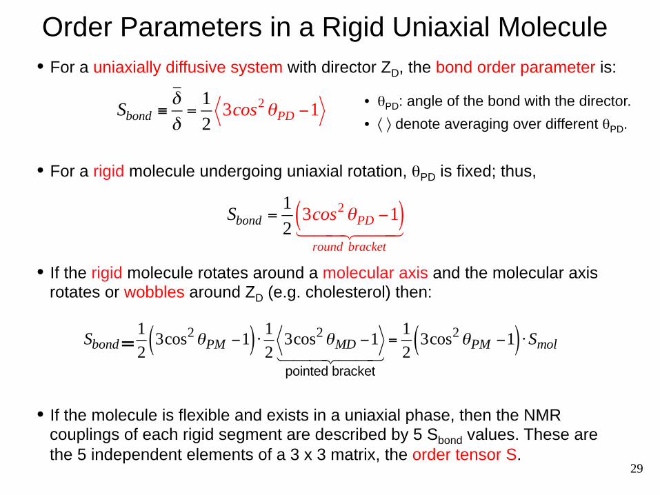
Sbond =

1

23cos2θPM −1( ) ⋅ 1

23cos2θMD −1

pointed bracket

=1

23cos2θPM −1( ) ⋅Smol

•  If the rigid molecule rotates around a molecular axis and the molecular axis rotates or wobbles around ZD (e.g. cholesterol) then:

•  For a rigid molecule undergoing uniaxial rotation, θPD is fixed; thus,

•  For a uniaxially diffusive system with director ZD, the bond order parameter is:

Sbond ≡δδ=

1

23cos2θPD −1

Sbond =1

23cos2θPD −1( )

round bracket

•  If the molecule is flexible and exists in a uniaxial phase, then the NMR couplings of each rigid segment are described by 5 Sbond values. These are the 5 independent elements of a 3 x 3 matrix, the order tensor S.

•  θPD: angle of the bond with the director.

•  〈〉 denote averaging over different θPD.

29

3030

Uniaxial Rotation of a Rigid Small Molecule

•  If amantadine rotates only around the molecular axis, then the average 2H quadrupolar coupling is:

3-fold axis Amantadine is rigid, and all bonds lie on a diamond lattice with tetrahedral angles relative to the molecular axis, ZM.

Relative to ZM:

•  If amantadine also rotates around the bilayer normal ZD:

• 12 CD bonds: 0.33⋅δ = 40 kHz

• 3 CD bonds : 1.0 ⋅δ =125 kHz

• 12 CD bonds : θPM = 70.5˚, 109.5˚

• 3 CD bonds : θPM = 0˚

δ = 12δ 3cos2θPM −1( )

δ = 12δ 3cos2θPM −1( ) ⋅ 1

23cos2θMD −1( )

= 12δ 3cos2θPM −1( ) ⋅Smol

31

2H quadrupolar coupling (kHz)

Amantadine Dynamics in Lipid Bilayers

Smol =±0.46 ⇒ θMD = 37˚, 80˚

Cady et al, Nature, 2010.

• 12 CD bonds: 0.33⋅δ = 40 kHz

• 3 CD bonds : 1.0 ⋅δ =125 kHz

Liquid-crystalline phase:

Smol ≈ 1 ⇒ θMD = 0°Gel phase:

32

Order Tensor: Flexible Molecules

•  Each rigid segment in the molecule has one S tensor, with its own principal axis system (where S is diagonal).

•  Each S matrix is traceless & symmetric, thus it has 5 independent elements, which requires 5 NMR couplings to determine.

There are many internally flexible biomolecules, e.g. multiple-domain proteins, RNA helices with hinge motions, sugars with flexible glycosidic linkages, and lipids.

δ =2

3Sij

Mσ ijM

i, j

∑

Sij ≡1

23cosθi

D cosθ jD −δij

: angle of the director with the i-th axis of the molecule θi

D

Averaged NMR couplings:

Saupe matrix:

•  Once the S tensor is known, one can calculate the motionally averaged NMR couplings for any direction in the rigid segment.

σ ij

M : interaction tensor elements in the molecule-fixed frame

33

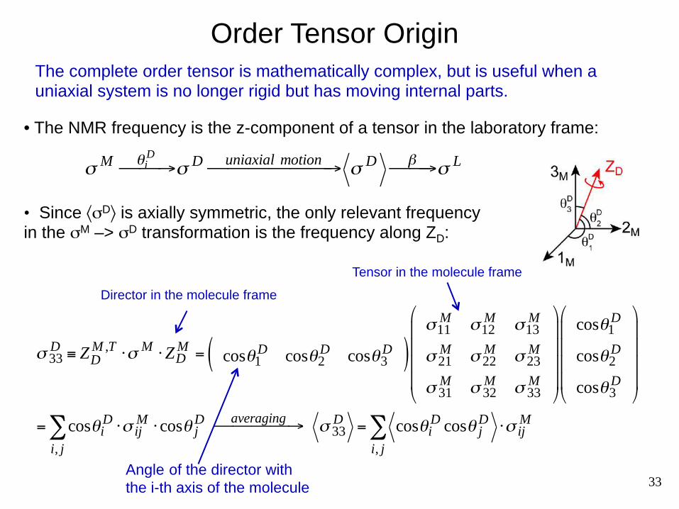
Order Tensor Origin

•  Since 〈σD〉 is axially symmetric, the only relevant frequency in the σM –> σD transformation is the frequency along ZD:

σ 33D ≡ ZD

M ,T ⋅σ M ⋅ZDM = cosθ1

D cosθ2D cosθ3

D( )σ11

M σ12M σ13

M

σ 21M σ 22

M σ 23M

σ 31M σ 32

M σ 33M

%

&

''''

(

)

****

cosθ1D

cosθ2D

cosθ3D

%

&

''''

(

)

****

= cosθiD ⋅σ ij

M ⋅ cosθ jD

i, j

∑ averaging, →,,, σ 33D = cosθi

D cosθ jD ⋅σ ij

M

i, j

∑

The complete order tensor is mathematically complex, but is useful when a uniaxial system is no longer rigid but has moving internal parts.

σ M θi

D

# →# σ D uniaxial motion# →##### σ D β# →# σ L

•  The NMR frequency is the z-component of a tensor in the laboratory frame:

Director in the molecule frame

Tensor in the molecule frame

Angle of the director with the i-th axis of the molecule

34

Sij ≡1

23cosθi

D cosθ jD −δij

σ 33D = cosθi

D cosθ jD ⋅σ ij

M

i, j

∑ =2

3

3

2cosθi

D cosθ jD − 1

2δij

Order tensor

⋅σ ijM

i, j

∑ +1

3δijσ ij

M

i, j

∑

A flexible molecule has multiple S tensors, one for each rigid segment.

δ ≡ σ 33D −σ iso =

2

3Sij

Mσ ijM

i, j

∑ ⇒ δ = 2

3Tr S iσ{ }

Once the S tensor is known, then one can calculate motionally averaged couplings along any direction.

Saupe matrix:

Some Order Tensor Derivations

Flexible RNAs: Order Tensors Reveal Domain Motion

Bailor…Al-Hashimi, Nature Protocol, 2007.

•  A rigid macromolecule has only one S tensor, and all motionally averaged NMR couplings (e.g. RDCs in solution NMR) fit to the same S tensor.

•  A flexible macromolecule has more than one S tensor. Aligning two different order tensors’ PAS systems allows the determination of the relative orientation of the two domains.

35

Trimannoside, 3 mannose rings connected by α(1,3) and α(1,6) glycosidic linkages.

Flexible Carbohydrates: RDCs & Order Matrices

Sauson-Flamsteed projection

•  Determinations of the S matrices for individual rigid fragments of a molecule allow both structural characterizations and assessments of internal motions between fragments.

•  The former arises because molecular fragments must share a common S tensor frame if a single rigid model exists;

•  The latter arises because the determined order parameters reflect overall averaging of the molecule as well as averaging due to internal motions.

Tian…Prestegard, JACS, 2001. 36

37

Relating Order Tensor to Order Parameter

Sbond ≡ S33

σ PAS =1

23cos2θPD −1( ) =δ δ

For uniaxially mobile proteins that are oriented along B0:

⇒ δ =δ ⋅S33

σ PAS =δ1

23cos2θ3, σ PAS

D −1( ) δ =σ PAS 2

3 Siiσ PAS ⋅σ ii

PAS

i

∑ = 23 δ ⋅S33

σ PAS − δ2 S11σ PAS + S22

σ PAS( )&'

()=

23 ⋅

32δ ⋅S33

σ PAS

Bond order parameter is the “projection” of the order tensor onto the bond.

θPD: angle of the director with respect to the bond

Thus, Sbond contains orientation information.

ω 0˚( )−ωiso =1

23cos2 0−1( )

due to alignment

δdue to motion

=δ = Sbond ⋅δ

38






39

Slow Motion: 2D Static Exchange NMR

2D spectrum S(ω1, ω2) is a joint probability: •  intensity distribution: motion geometry. •  geometry encoded in a single angle β for a uniaxial interaction. •  tm dependence –> correlation time.

S (ω1,ω2 ;β) (for η=0)

Schmidt-Rohr and Spiess, 1994.

1D Stimulated Echo: Time-Domain Exchange

•  1D analog of 2D exchange: t1 = τ.

•  Allows fast determination of τc by varying tm without multiple 2D.

1D time signal: t2 = t1 = te. •  Segments without frequency change: ω(θ1) = ω(θ2) = ω (diagonal).

M te( ) = e−iωte ⋅ eiωte = 12 scans

•  Segments with frequency change:

M te( ) = e−iω θ1( )te ⋅ eiω θ2( )te = e

iω θ2( )−ω θ1( )%& '(te →long tm

0

1D stimulated echo intensity = 2D diagonal intensity

2D time signal:

f t1,t2( ) = cosω θ1( )t1 − isinω θ1( )t1$% &'⋅ eiω θ2( )t2 = e−iω θ1( )t1 ⋅ eiω θ2( )t2

powder averaging

40

41

1D Stimulated Echo Under MAS: CODEX

•  180˚ pulse train recouples X-spin CSA.

•  90˚ storage and read-out pulses are phase-cycled together.

•  After the 2nd recoupling period, the MAS phase for 2 scans is:

Φ1 =N

2ω1 t( )dt

0

tr 2∫ − ω1 t( )dt

tr 2

tr∫( ) = N ω1 t( )dt0

tr 2∫

Φ2 =N

2− ω2 t( )dt

0

tr 2∫ + ω2 t( )dt

tr 2

tr∫( ) = −N ω2 t( )dt0

tr 2∫

•  No motion: ω1 = ω2, → cos(Φ1+Φ2) = 1, full echo. •  With motion: ω1 ≠ ω2, → cos(Φ1+Φ2) < 1, reduced echo.

Rec: y y

deAzevedo et al, J. Chem. Phys., 112, 8988 (2000).

cosΦ1 cosΦ2 − sinΦ1 sinΦ2 = cos Φ1+Φ2( ) = cos Φ2 − Φ1( )

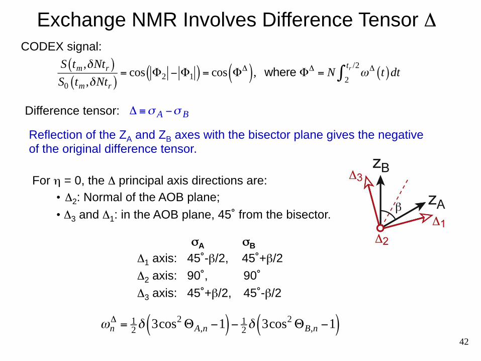
Exchange NMR Involves Difference Tensor Δ

Δ ≡σ A −σ B

For η = 0, the Δ principal axis directions are: •  Δ2: Normal of the AOB plane; •  Δ3 and Δ1: in the AOB plane, 45˚ from the bisector.

σA σB

Δ1 axis: 45˚-β/2, 45˚+β/2 Δ2 axis: 90˚, 90˚ Δ3 axis: 45˚+β/2, 45˚-β/2

ωnΔ = 1

2δ 3cos2ΘA,n −1( )− 12δ 3cos2ΘB,n −1( )

CODEX signal:

S tm ,δNtr( )S0 tm ,δNtr( )

= cos Φ2 − Φ1( ) = cos ΦΔ( ), where ΦΔ = N ωΔ t( )dt2

tr /2∫

Difference tensor:

Reflection of the ZA and ZB axes with the bisector plane gives the negative of the original difference tensor.

42

ω2Δ =ωA,2 −ωB,2 = 0

ω1Δ =ωA,1 −ωB,1 =

32δ ⋅ 1

2cos 90°−β( )− cos 90°+β( )'( )*= 3

2δ sinβ

ω3Δ =ωA,3 −ωB,3 =

32δ ⋅ 1

2cos 90°+β( )− cos 90°−β( )'( )*= − 3

2δ sinβ

43

CODEX is Sensitive to Small-Angle Reorientations

€

€

⇒ ηΔ = 1

ω33Δ − ω11

Δ = 3δ ⋅ sinβ = ω33 − ω11 ⋅2 sinβ

•  CODEX signal scales ~ sinβ, which is ~β for small angles. •  Usual angular dependence is (3cos2β-1)/2, which scales ~ β2 .

For ZA : For ZB

ωA,2 =12δ 3cos2 90°−1( ) = − 1

2δ ωB,2 =

12δ 3cos2 90°−1( ) = − 1

2δ

ωA,1 =12δ 3cos2 45°−β 2( )−1( ) ωB,1 =

12δ 3cos2 45°+β 2( )−1( )

ωA,3 =12δ 3cos2 45°+β 2( )−1( ) ωB,3 =

12δ 3cos2 45°−β 2( )−1( )

CODEX: Reorientation Angles & Number of Sites

E tm ,δNtr( ) = R β( )ε δNtr;β( )dt ⋅dβ0

90°∫

€

ε δNtr;β( )

ΔS

S0tm >> τ c,δNtr >>1( )

=1−1

M

Jump motions:

3-site jump

Isotropic jump

Isotropic diffusion

Uniaxial rotation

Schmidt-Rohr et al, Encyclop NMR, 9, 633 (2002).

2/3

44

Dipolar CODEX Use dipolar coupling instead of CSA to probe orientational change:

•  15N-1H: Use perdeuterated proteins to minimize 1H spin diffusion

•  13C-1H and 15N-1H: decouple 1H-1H couplings in protonated proteins to suppress 1H spin diffusion

•  15N-13C: ~1 kHz couplings, probes τc >> 1 ms

McDermott et al;

Krushelnitscky, Saalwächter, Reichert, et al.

45

Phase Cycling:

Selecting Desired Signals and Removing Artifacts

46

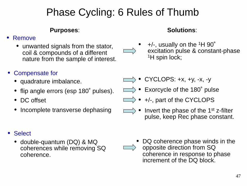
Solutions:

•  +/-, usually on the 1H 90˚ excitation pulse & constant-phase 1H spin lock;

•  CYCLOPS: +x, +y, -x, -y

•  Exorcycle of the 180˚ pulse

•  +/-, part of the CYCLOPS

•  Invert the phase of the 1st z-filter pulse, keep Rec phase constant.

•  DQ coherence phase winds in the opposite direction from SQ coherence in response to phase increment of the DQ block.

Phase Cycling: 6 Rules of Thumb

•  Remove •  unwanted signals from the stator,

coil & compounds of a different nature from the sample of interest.

Purposes:

•  Compensate for •  quadrature imbalance.

•  flip angle errors (esp 180˚ pulses).

•  DC offset

•  Incomplete transverse dephasing

•  Select •  double-quantum (DQ) & MQ

coherences while removing SQ coherence.

47

•  The 1H spin lock phase should be perpendicular to the 90˚ excitation phase.

•  13C spin lock phase is independent of the 1H spin lock phase.

•  The 1H M vs B1 relation is inverted every other scan to cause inversion of the 13C M and the receiver phase, so that M of 13C spins uncoupled or weakly coupled to 1H can be canceled (if desired).

•  The relative orientation between M and B1 must be the same between the two channels.

Phase Cycling of CP (1H⇒X, 15N⇒13C, etc)

Rec +x-x

48

Phase Cycling of z Mixing Pulses & Echo Pulses

•  Z-filter: 1st 90˚ phase inverted against M every other scan while the 2nd 90˚ phase remains constant;

•  The 2nd 90˚ phase does not have to be parallel to the 1st 90˚ phase.

•  The inversion of the desired M and the receiver removes undestroyed transverse M.

Z-filter

•  Exorcycle of the 180˚ pulse compensates for flip angle (β) errors. Even when β≠180˚, M refocuses with the correct phase, except for an intensity scaling of (1-cosβ)/2.

Exorcycle: Bodenhausen et al, JMR, 1977. Application in REDOR: Sinha et al, JMR, 2004.

Echo

49

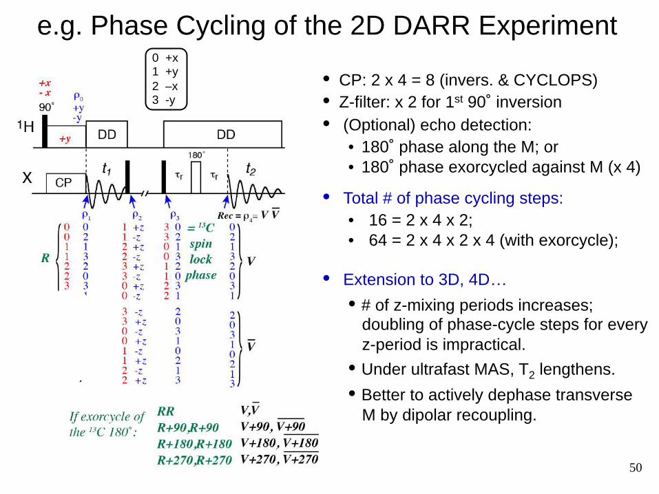
e.g. Phase Cycling of the 2D DARR Experiment

•  CP: 2 x 4 = 8 (invers. & CYCLOPS) •  Z-filter: x 2 for 1st 90˚ inversion •  (Optional) echo detection:

•  180˚ phase along the M; or •  180˚ phase exorcycled against M (x 4)

•  Total # of phase cycling steps: •  16 = 2 x 4 x 2; •  64 = 2 x 4 x 2 x 4 (with exorcycle);

•  Extension to 3D, 4D…

• # of z-mixing periods increases; doubling of phase-cycle steps for every z-period is impractical.

• Under ultrafast MAS, T2 lengthens.

• Better to actively dephase transverse M by dipolar recoupling.

0 +x 1 +y 2 –x 3 -y

50

Summary

Motions are ubiquitous in biological molecules.

•  Fast motions average the interaction tensors and narrow the spectra.

•  Based on symmetry, the sum (Σ) NMR tensors and spectral lineshapes of several motions can be analytically predicted.

•  Fast motions can be measured using 2D experiments that resolve dipolar couplings by chemical shifts (DIPSHIFT, LG-CP, etc).

•  Slow motions can be measured in terms of 2D exchange cross peaks or stimulated echo intensities.

•  The geometry of slow motion is described by difference tensors.

•  CSA and dipolar CODEX is a robust exchange technique under MAS.

•  Order parameters & order tensors give information on whole-body motions and internal motions.

•  6 rules of thumb allow the construction of phase cycles in many NMR experiments.

51

Funding: NIH, DOE, MIT

Acknowledgement

Tuo Wang Shu (Aaron) Liao Jon Williams Byungsu Kwon Myungwoon Lee Matt Elkins Pyae Phyo Marty Gelenter Shiva Mandala Dr. Hongwei Yao

Current Hong group

52

Appendix

54

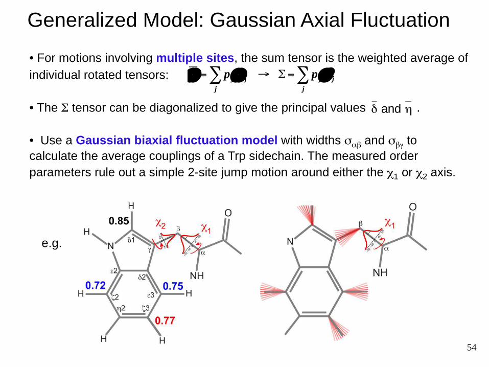
Generalized Model: Gaussian Axial Fluctuation

•  For motions involving multiple sites, the sum tensor is the weighted average of individual rotated tensors:

•  The Σ tensor can be diagonalized to give the principal values .

•  Use a Gaussian biaxial fluctuation model with widths σαβ and σβγ to calculate the average couplings of a Trp sidechain. The measured order parameters rule out a simple 2-site jump motion around either the χ1 or χ2 axis.

δ and η

ω = p jω jj

∑ → Σ = p jσ jj

∑

e.g.

55

Motion of the Gating Tryptophan in the M2 Channel

σαβ ≈ 30 ̊

σβγ ≈ 15˚

56

• In the doubly rotating frame:

H =ω1I Ix +ω1SSx

rf part +ΔωI Iz +ωIS t( ) IzSz

I−S dip

+ωII t( ) 3Izi Iz

j − I i ⋅ I j( )I-I dip

€

€

where ωIS t( ) = 2δ C1 cos ωr t + γ( ) + C2 cos 2ωr t + 2γ( )[ ]

LG-CP Average Hamiltonian

H IST =ωIS t( ) sinθmIx cosωeff ,I t − sinθmIy sinωeff ,I t − cosθmIz( )

• Sx cosω1,St −Sy sinω1,St( )

=ωIS t( )IxSx cosωeff ,I t cosω1,St sinθm + IySy sinωeff ,I t sinω1,St sinθm

−IxSy − IySx − IzSx cosω1,St cosθm + IzSy sinω1,St cosθm

$

%&&

'

())

• Transform to a tilted frame,

H T = RHR−1, where R=e−iθmIy e

−i π2 Sy ,

H T =ωeff ,I Iz +ω1SSz

rf part

+ωIS t( ) sinθmIx − cosθmIz( )Sx +H IIT

• Transform to the interaction frame of the rf pulses, H IST = e

iHrf t ⋅H IST ⋅ e

−iHrf t

H IST =

1

2δ sinθm

IxSx + IySy( )C1 cosγ −

IySx − IxSy( )C1 sinγ

%

&

''

(

)

**=

1

2δ sinθmC1 i Ix

23( ) cosγ − Iy23( ) sinγ%

&'()*

The average Hamiltonian contains non-zero terms such as:

IxSx ⋅ ωIS t( ) ⋅ cosωeff ,I t ⋅ cosω1,St ⋅sinθm

= IxSx ⋅ 2δC1 cos ωrt +γ( ) ⋅ cosωeff ,I t ⋅ cosω1,St ⋅sinθm = IxSx ⋅1

2δ sinθm ⋅C1 cosγ

H IST

0( )= 1

2δ sinθmC1

ωIS,LG

i Ix23( ), Iy

23( ), Iz23( )( )

I 23( )

cosγ

sinγ

0

%

&

'''

(

)

***

BIS,LG

The average heteronuclear coupling is the scalar product between ZQ spin operators and a tilted effective LG field:

57

ZQ spin operators: Ix

23( ) ≡ IxSx + IySy, Iy23( ) ≡ I y Sx − IxSy, Iz

23( ) ≡ 12

I z−Sz( )

ωeff ,I −ω1,S =±ωrUnder the sideband matching condition:

LG-CP: 1H-1H Homonuclear Decoupling

€

HII = ωII t( ) 3I z I z − I⋅ I% & ' )

HIIT = ωII t( ) 3 I z cosθm − I x sinθm( ) I z cosθm − I x sinθm( ) − I⋅ I[ ]

H IIT =ωII t( )

3 Iz cosθm − Ix sinθm cosωeff t + Iy sinθm sinωeff t( ) ⋅Iz cosθm − Ix sinθm cosωeff t + Iy sinθm sinωeff t( )− I ⋅ I

%

&

''

(

)

**

Time average,

58

H II

T , 0( )= ωII t( ) 3

IzIz cos2θm + IxIx sin2θm cos2ωeff t +

IyIy sin2θm sin2ωeff t

#

$

%%

&

'

((− I ⋅ I

+

,

--

.

/

00

= ωII t( ) 3 IzIz ⋅1

3 + IxIx ⋅

2

3⋅1

2 + IyIy ⋅

2

3⋅1

2

#

$%

&

'(− I ⋅ I

+

,-

.

/0

= ωII t( ) IzIz + IxIx + IyIy( ) − I ⋅ I+,

./ =0

Magic zero

Transform to the interaction frame of the rf pulses:

59

Variants of the LG-CP Experiment

Colicin Ia channel domain: soluble and membrane-bound states:

Constant-time version removes T1ρ relaxation effects

Hong, Yao, Jakes and Huster, J. Phys. Chem, 106, 7355 (2002). Yao, McMillian, Conticello and Hong, Magn. Reson. Chem., 42, 267 (2004).

60

Sensitivity-Enhanced LG-CP

Gln

PILGRIM

Hong, Yao, Jakes and Huster, J. Phys. Chem, 106, 7355 (2002). Lorieau and McDermott, JACS,128, 11505 (2006).

€

ρ 0( ) = I z(14) + I z

(23)

ρ 0( ) = I z − Sz = 2I z(23)

§  Original LG-CP:

§  PILGRIM:

Theoretical enhancement factor = 2

ρLG−CP t( ) = 1

2Iz 1+ cosωIS,LGt( )+ 1

2Sz 1− cosωIS,LGt( )

ρPILGRIM t( ) = Iz cosωIS,LGt − Sz cosωIS,LGt

61

Properties of Order Tensor & Order Parameter

Sbond ≡ S33

σ PAS =1

23cos2θPD −1( ) =δ δ

•  For 0˚-oriented uniaxially mobile systems,

•  Thus, Sbond contains the same information as oriented-membrane spectra. ω 0˚( )-ωiso =

12δ 3cos2 0˚−1( ) = δ

•  The S tensor is traceless & symmetric.

•  Thus, the S tensor has 5 independent elements, which require 5 independent NMR couplings.

•  Bond order parameter is the “projection” of the order tensor onto the bond.

Siii

∑ = 32 cos2θi

D

i

∑ − 32 = 0 cosθi cosθ j = cosθ j cosθi( )

⇒ δ =δ ⋅S33

σ PAS =δ1

23cos2θ3, σ PAS

D −1( ) δ =σ PAS 2

3 Siiσ PAS ⋅σ ii

PAS

i

∑ = 23 δ ⋅S33

σ PAS − δ2 S11σ PAS + S22

σ PAS( )&'

()=

23 ⋅

32δ ⋅S33

σ PAS

θ3, σ PASD =θPD

Intermediate Motion – Chemical Exchange

ν (Hz)

k ≈ ωA −ωB

Intermediate motion can be measured using:

•  Relaxation times: e.g. exchange-induced T2

•  Asymmetry in DIPSHIFT time signal

Isotropic shift exchange: k ≈ π 2Δνiso2 T2

* 2 Exchange induced T2

∗ = R2,ctrl − R2,ex( )−1

•  Isotropic liquids: mainly averaging isotropic chemical shifts

•  For anisotropic solids, averaging all anisotropic frequencies; also need to consider motional interference with

•  1H dipolar decoupling (dipolar modulation)

•  MAS (CSA modulation)

Decoupling and MAS can be accounted for by numerical simulations.

62

Intermediate Motion Causes DIPSHIFT Asymmetry

Slow, 10-1

Intermediate, 104 s-1

Fast, 106 s-1

Intermediate, 104 s-1

2-site jump with βR=64˚

deAzevedo et al, JCP, 2008.

105 s-1

103 s-1

•  Full spin dynamics simulations.

•  Only single DIPSHIFT manifests the asymmetry.

•  Asymmetry independent of imperfect 1H decoupling and effective T2.

63

k = 104 s-1 k = 105 s-1 k = 106 s-1

fast Intermediate Slow-intermediate

High mid point, low final intensity.

Low mid point, low final intensity.

Larger Reorientations Cause Stronger Asymmetry

deAzevedo et al, JCP, 2008. 64

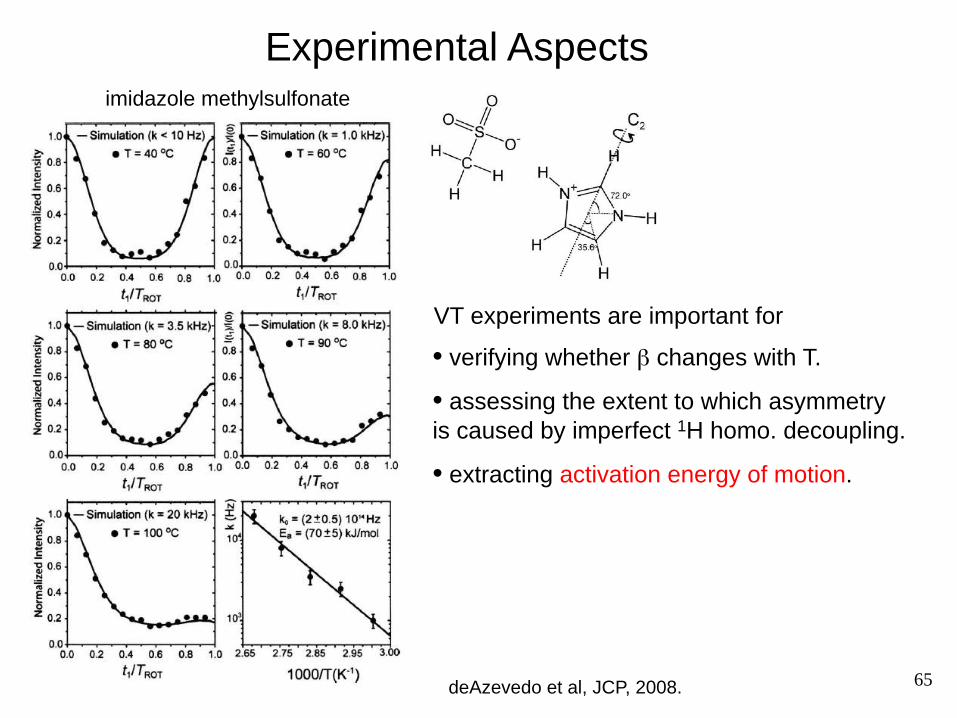
Experimental Aspects

•  verifying whether β changes with T.

•  assessing the extent to which asymmetry is caused by imperfect 1H homo. decoupling.

•  extracting activation energy of motion.

VT experiments are important for

imidazole methylsulfonate

deAzevedo et al, JCP, 2008. 65

Documents

Solid-State NMR Studies of Biomolecular Motion