1

Sliding Mode Control: An Approach To Regulate Nonlinear Chemical Processes

Oscar Camacho Carlos A. Smith Departamento de Circuitos y Medidas Chemical Engineering Department

Universidad de Los Andes University of South Florida Mérida 5101. Venezuela Tampa – Florida. USA

Abstract A new approach for the design of Sliding Mode Controllers based on a first-order-plus-deadtime model of the process is developed. This approach results in a fixed structure controller with a set of tuning equations as a function of the characteristic parameters of the model. The controller performance is judged by simulations on two nonlinear chemical processes. Keywords: Sliding Mode Control, Variable Structure Control, Nonlinear Chemical Processes.

1. Introduction Sliding Mode Control (SMC) is a robust and simple procedure to synthesize controllers for linear and nonlinear processes. To develop a Sliding Mode Controller, SMCr, knowledge of the process model relating the controlled variable, XBCB(t), to the manipulated variable, U(t), is necessary. However, there are two problems with the use of a model as far as chemical processes are concerned. First, the development of a complete model is difficult due mainly to the complexity of the process itself, and to the lack of knowledge of some process parameters. Second, most process models relating the controlled and the manipulated variables are of higher-order. Generally, the SMC procedure produces a complex controller, which could contain four or more parameters resulting in a difficult tuning job. Therefore, the use of the traditional procedures of SMC presents disadvantages in their application to chemical processes. An efficient alternative modeling method for process control is the use of empirical models, which use low order linear models with deadtime. Most times, first-order-plus deadtime (FOPDT) models are adequate for process control analysis and design. But, these reduced order models present uncertainties arising from imperfect knowledge of the model, and the process nonlinear effects contribute to performance degradation of the controllers. Conventional controllers, such as PID, Lead-Lag or Smith Predictors, are sometimes not sufficiently versatile to compensate for these effects. Thus, a SMCr could be designed to control nonlinear systems with the assumption that the robustness of the controller will compensate for modeling errors arising from the linearization of the nonlinear model of the process. The aim of this paper is to design a SMCr based on a first-order-plus-deadtime (FOPDT) model of the actual process. The overall idea is to develop a general SMCr, which can be used for self-regulating chemical processes. The parameters of the model, process gain, K, process time constant, τ , and process deadtime, tB0 B, are used to obtain the initial estimates of the tuning terms in the SMCr.B

This article is organized as follows. Section 2 briefly presents the process model. Section 3, presents some basic concepts of the SMC method. Section 4 shows the procedure to design a SMCr using the FOPDT model. Tuning equations for the controller are also given in this section. In Section 5 the simulation of the SMCr for two nonlinear chemical processes is presented. Section 6 concludes the paper.

2

2. Process Model The process reaction curve, Figure 1, is an often-used method for identifying dynamic models [1]. It is simple to perform, and provides adequate models for many applications. The curve is obtained by introducing a step change in the output from the controller and recording the transmitter output.

[Figure 1] From the process curve shown in the figure, and the procedure presented in the reference, the numerical values of the terms in the FOPDT model given in Eq. 1 are obtained

1)()( 0

+=

−

sKe

sUsX st

τ (1)

where X(s) is the Laplace transform of the controlled variable, the transmitter output, and U(s) is the Laplace transform of the manipulated variable, the controller output. Both X(s) and U(s) are deviation variables. In this paper we use the unit of X(s) as fraction of the transmitter output, fraction TO; the unit of U(s) is fraction of the controller output, fraction CO. K, tB0B and τ were previously defined.

3. Basic Concepts about Sliding Mode Control Sliding Mode Control is a technique derived from Variable Structure Control (VSC) which was originally studied by [2]. The controller designed using the SMC method is particularly appealing due to its ability to deal with nonlinear systems and time-varying systems [3-5]. The robustness to the uncertainties becomes an important aspect in designing any control system. The idea behind SMC is to define a surface along which the process can slide to its desired final value; Figure 2 depicts the SMC objective. The structure of the controller is intentionally altered as its state crosses the surface in accordance with a prescribed control law. Thus, the first step in SMC is to define the sliding surface S(t). S(t) is chosen to represent a desired global behavior, for instance stability and tracking performance; The S(t) selected in this work, presented by [4], is an integral-differential equation acting on the tracking-error expression

∫⎟⎠⎞

⎜⎝⎛ +=

tn

dttedtdtS

0

)()( λ (2)

where e(t) is the tracking error, that is, the difference between the reference value or set point, R(t), and the output measurement, X(t), or e(t) = R(t) - X(t). λ is a tuning parameter, which helps to define S (t); This term is selected by the designer, and determines the performance of the system on the sliding surface, n is the system order

[Figure 2]

The objective of control is to ensure that the controlled variable be equal to its reference value at all times, meaning that e (t) and its derivatives must be zero. Once the reference value is reached, Eq. 2 indicates that S

3

(t) reaches a constant value. To maintain S (t) at this constant value, meaning that e (t) is zero at all times; it is desired to make

0)(=

dttdS

(3)

Once the sliding surface has been selected, attention must be turned to design of the control law that drives the controlled variable to its reference value and satisfies Eq. 3. The SMC control law, U (t), consists of two additive parts; a continuous part, U BCB (t), and a discontinuous part, U BD B (t), [6]. That is

)()()( tUtUtU DC += (4) The continuous part is given by

( ))(),()( tRtXftU C = (5) where f (X (t), R(t)) is a function of the controlled variable, and the reference value. The discontinuous part, U BD B (t), incorporates a nonlinear element that includes the switching element of the control law. This part of the controller is discontinuous across the sliding surface.

δ+=

)()()(

tStSKtU DD (6)

where KBD B is the tuning parameter responsible for the reaching mode. δ is a tuning parameter used to reduce the chattering problem. Chattering is a high-frequency oscillation around the desired equilibrium point. It is undesirable in practice, because it involves high control activity and also can excite high-frequency dynamics ignored in the modeling of the system [3, 4, 6]. In summary, the control law usually results in a fast motion to bring the state onto the sliding surface, and a slower motion to proceed until a desired state is reached.

4. SMCr Synthesis from an FOPDT Model of the Process This section presents the development of a general SMCr, for self-regulating processes, using a first-order-plus-deadtime (FOPDT) process model. The FOPDT model is an approximation to the actual higher-order model. The development of this controller significantly simplifies the application of sliding mode control theory to chemical processes. The literature reviewed does not reveal a simple and practical method to apply SMC to process with dead time [7-9]. In this chapter, a SMCr structure based on the FOPDT model of the actual process is designed. Thus, the first step is to propose a way to handle the deadtime term The deadtime can be approximated in two different ways. A first-order Taylor series approximation to the deadtime term produces

11

0

0

+≅−

ste st (7)

The above approximation can also be written as a first-order Padé Approximation

4

st.st.

e st

0

0

501501

0

+−

≅− (8)

Figure 3 shows a comparison among the deadtime term and the first-order Taylor series and Padé Approximations. The figure shows that the Padé Approximation works very well between 0 and 1 but beyond the approximation brakes down. On other hand, the Taylor series approximation improves as tB0 B increases. [Figure 3] In [10] is shown that the first-order Taylor approximation or the Padé approximation can be considered as good approximations for the deadtime term for chemical processes. The next section shows the development of a SMCr using both approximations. 4.1 SMCr Development Based on a First-Order Taylor Series Approximation In this section a SMCr is developed based on the first-order Taylor series expansion. Additionally, a rule to choose the tuning parameters will also be presented. Substituting Eq. 7 into Eq. 1 produces

1)+st1)(+s(K

U(s)X(s)

oτ≅ (9)

In differential equation form

KU(t)=X(t)+dt

dX(t))+t(+dtX(t)dt o2

2

o ττ (10)

and since this is a second-order differential equation, n = 2, from Eq. 2 S (t) becomes

∫++=t

dttetedt

tdetS0

01 )()()()( λλ (11)

Where λλ 21= and 20 λλ =

From Eq. 3

0)()()()(012

2

=++= tedt

tdedt

teddt

tdSλλ (12)

Substituting the definition of the error, e(t) = R(t) - X(t), into the first two terms of the above equation gives

0)()()()()(012

2

2

2

=+⎟⎠⎞

⎜⎝⎛ −+− te

dttdX

dttdR

dttXd

dttRd

λλ (13)

5

Solving for the highest derivative from Eq. 10, substituting it into the Eq. 13, and solving for U(t) provides the continuous part of the controller

⎥⎥⎦

⎤

⎢⎢⎣

⎡++++⎟⎟

⎠

⎞⎜⎜⎝

⎛−

+⎟⎠

⎞⎜⎝

⎛=

dttdR

dttRdte

ttX

dttdX

tt

Kt

tU C)()()()()()( 12

2

00

10

00 λλτ

λτττ

(14)

This procedure, involving Eqs. 11, and 13, to obtain the expression for the continuous part of the controller is known in the SMC theory as the equivalent control procedure [2]. In [11] is shown that the derivatives of the reference value can be discarded, without any effect on the control performance, resulting in a simpler controller. Thus,

⎥⎥⎦

⎤

⎢⎢⎣

⎡++⎟⎟

⎠

⎞⎜⎜⎝

⎛−

+⎟⎠

⎞⎜⎝

⎛= )()()()( 0

01

0

00 tet

tXdt

tdXt

tK

ttU C λ

τλ

τττ

(15)

U BCB(t) can be simplified by letting,

ττ

λ0

01 t

t += (16)

It has been shown that this choice for λ B1B is the best for the continuous part of the controller [11]. To assure that the sliding surfaces behaves as a critical or overdamped system, λ B0B should be

4

21

0λ

λ ≤ (17)

Then, the complete SMCr can be represented as follows

δλ

ττ

++⎥

⎦

⎤⎢⎣

⎡+⎟

⎠

⎞⎜⎝

⎛=

)()()()()( 0

0

0

tStSKte

ttX

Kt

tU D (18a)

with

⎥⎦

⎤⎢⎣

⎡++−= ∫

t

dttetedt

tdXKsigntS

001 )()(

)()()( λλ (18b)

Equations 18a and 18b constitute the controller equations to be used. These equations present advantages from process control point of view, first they have a fixed structure depending on the λ’s parameters and the characteristic parameters of the FOPDT model, and second the action of the controller is considered in the sliding surface equation, by including the term sign(K), in Eq. 18b. Note, that sign(K) only depends on the static gain, therefore it never switches. From an industrial application perspective, Eq. 18b represents a PID algorithm [12]. To complete the SMCr, it is necessary to have a set of tuning equations. For the tuning equations as first estimates, using the Nelder-Mead searching algorithm [13], the following equations were obtained [11]. • For the continuous part of the controller and the sliding surface

6

ττ

λ0

01 t

t += [=] [time]P

-1P (19a)

2

0

00 4

1⎟⎟⎠

⎞⎜⎜⎝

⎛ +=

ττ

λt

t [=] [time]P

-2P (19b)

• For the discontinuous part of the controller

76.0

0

51.0⎟⎟⎠

⎞⎜⎜⎝

⎛=

tKK D

τ[=] [fraction CO] (19c)

112.068.0 λδ DKK+= [=] [fraction TO/time] (19d)

Eqs. 19c and 19d are used when the signals from the transmitter and controller are in fractions (0 to 1). Sometimes, the control systems work in percentages that is, the signals are in % (0 to 100) of range. In these cases the values of KD andδ are multiplied by 100. 4.2 SMCr development based on the Padé Approximation This section contains the development of the control law when the deadtime term of the FOPDT process model is approximated by the Padé approximation, Eq. 8. The procedure followed in this section is similar to that one presented in the previous part. Substituting Eq. 8 into Eq. 1, gives

s)t + 2 ( ) 1 + s ( s)t - 2 (K

(s) U(s) X C

0

0

τ≅ (20)

Using a similar procedure as shown above, the continuous part of the controller, Uc(s), is

⎥⎥⎥⎥⎥

⎦

⎤

⎢⎢⎢⎢⎢

⎣

⎡⎥⎦

⎤⎢⎣

⎡⎟⎟⎠

⎞⎜⎜⎝

⎛

t2 - s

(s) e +(s) X t2 + s -

tt + 2 + R(s) s) + s(

K - = (s) U

C12

C

0

00

10

0 λτ

λτ

τλ

τ (21)

Eq. (21) has a pole (+2/tB0B) on the right side of the complex plane. Thus, the continuous part of the controller contains an unstable term. Eq. (20) represents a nonminimun phase system. Hence, the equivalent control procedure applied directly over this kind of systems produce unstable controllers. An approach to solve the previous problem, and that permit the use of SMC to nonminimun phase processes is presented in [10]. In summary, up to now, the synthesis of a SMCr has been shown from the linearization of a nonlinear chemical process. The linear model representing the nonlinear chemical process is an FOPDT model. The characteristic parameters of the FOPDT model also are used in the tuning equations Thus, from the previous results, the controller equation to be used is that obtained from the Taylor Series Approximation. The next part illustrates the controller performance.

7

5. Simulation Results This section simulates the control performance of the SMCr designed and given in Eqs. 18a and 18b. The first process, a mixing tank, compares the performance of the SMCr with respect to a PID controller. The second process, a chemical reactor, presents further performance characteristics. 5.1 Mixing Tank Consider the mixing tank shown in Figure 4. The tank receives two streams, a hot stream, W B1B (t), and a cold stream, W B2 B(t). The outlet temperature is measured at a point 125 ft downstream from the tank. The following assumptions are accepted •The liquid volume in the tank is considered constant •The tank contents are well mixed •The tank and the pipe are well insulated. The temperature transmitter is calibrated for a range of 100P

oPF to 200 P

oPF. Table 1 shows the steady-state

conditions and other operating information.

[Figure 4]

The following equations constitute the process model •Energy balance around mixing tank

( )dt

)t(dTCvV)t(T)t(Cp)t(W)t(W)t(T)t(Cp)t(W)t(T)t(Cp)t(W 3

33321222111 ρ=+−− (22)

•Pipe delay between the tank and the sensor location

(t))t-(t)(tT=(t)T o34 (23) •Transportation lag or delay time

(t)W+(t)WLA=t

21

ρ0 (24)

•Temperature Transmitter

⎥⎦⎤

⎢⎣⎡ −

− )t(TO)t(T1=dt

dTO(t)T 100

1004

τ (25)

• Valve position

p

Vpp

dV (t)dt

=1

m(t) -V (t)τ

[ ] (26)

•Valve equation

2 VL p f vW (t) = C V (t) G P50060

∆ (27)

•Sliding Mode Controller (SMCr)

8

U(t)= U (t)+U (t)c D (28) where WB1 B (t) = mass flow of hot stream, lb/min WB2 B (t) = mass flow of cold stream, lb/min Cp = liquid heat capacity at constant pressure, Btu/lb-°F Cv = liquid heat capacity at constant volume, Btu/lb-°F T B1B (t) = hot flow temperature, °F T B2 B(t) = cold flow temperature, °F T B3B (t) = liquid temperature in the mixing tank, °F T B4B (t) = equal to TB3 B(t) delayed by tBoB, °F tBo B = deadtime or transportation lag, min ρ = density of the mixing tank contents, lbm/ftP

3

V = liquid volume, ftP

3

TO (t) = transmitter output signal on a scale from 0 to 1 VBp B (t) = valve position, from 0 (valve closed) to 1 (valve open) m (t) = fraction of controller output, from 0 to 1 B CVL = Bvalve flow coefficient, gpm/psiP

1/2

G Bf = Bspecific gravity, dimensionless ∆ Pv = pressure drop across the valve, psi τ BT = Btime constant of the temperature sensor, min τ BVp = Btime constant of the actuator, min A = pipe cross section, ftP

2P

L = pipe length, ft B B

Table 1. Design parameters and steady-state values

Variable Value Variable Value W B1B 250.00 lb/min V 15 ftP

3P

W B2B 191.17 lb/min TO 0.5 Cp B1B B B 0.8 Btu/lb-°F Vp 0.478 Cp B2B 1.0 Btu/lb-°F

B CVLB

12 gpm / psiP

1/2P

Cp B3B, Cv B3B 0.9 Btu/lb-°F ∆ Pv 16 psi Set point 150 °F τ BT B 0.5 min

TB1B 250 °F τ Bvp B 0.4 min

TB2B 50 °F A 0.2006 ftP

2P

TB3B 150 °F L 125 ft ρ 62.4 lb / ftP

3P m 0.478 CO

Following the procedure, presented in Section 2, to obtain the parameters of the FOPDT model yields: K = - 0.78 fraction TO/fraction CO, τ = 2.32 min., and tB0 B= 2.97 min. Using these values the tuning parameters for the SMCr are

min/TOfraction.min.

COfraction.Kmin. D

7190 ; 1470

540 ; 76702

0

11

==

==−

−

δλ

λ

The tuning parameters for the PI controller are 50.KC −= and τ I = 2 32. min , using the tuning formulas for Dahlin synthesis, which produce smoother responses than Ziegler-Nichols tuning equations, working better for process with deadtime [1]. Note that the comparison is done using the initial tuning parameters for both controllers, to show the good performance obtained for the SMCr initial tuning equations, but they can be adjusted, fine tuning, until acceptable control performance be obtained.

9

Please note that the controller equations, Eqs. 18a and 18b, were developed using deviation variables. The following changes the “deviation variables” in the controller to “actual variables”

mm(t))t(U - =

TOTO(t) - )t(X = and e (t) = R(t) - TO(t) where m(t) is the controller output, in fraction CO, TO(t) is the transmitter output, in fraction, and R(t) is the reference value, or set point, fraction TO. The overbars indicate steady-state values. Since the process gain is negative, sign (K) is negative, the controller equation to be used is

δλ

ττ

+|)t(S|)t(SK+e(t)+)TO-(TO(t)

t1

Kt-m=m(t) D

⎥⎦

⎤⎢⎣

⎡0

0

0 (18a)

with

dttetedt

tdTOtSt

∫−−=0

01 )( )( )()( λλ (18b)

Figure 5 shows the response of the temperature, T t4 ( ) , when the flow of hot water changes from 250 lb/min to 200 lb/min, then to 175 lb/min, to 150 lb/min, and finally to 125 lb/min. The curves clearly show that as the operating conditions change, the performance of the PID controller degrades, while that of the SMCr maintains its performance and stability. In this case, as the flow of hot water decreases, with a corresponding decrease in cold water, the deadtime between the tank and the sensor increases. This increase in deadtime certainly adversely affects the performance of the PID controller. To recover stability, new tunings are required for the PI controller while none are required for the SMCr.

[Figure 5]

In spite of the controller was synthesized using a Taylor approximation and the tuning equations, Eqs. 19a to 19d, are empirical, the proposed method can be successfully used in processes with a deadtime to time constant ratio larger than one. In our experience, they can be applied for tB0B/τ around of 3.

5.2 Chemical Reactor The reactor shown in Fig. 6 is a continuous stirred tank where the exothermic reaction A → B takes place. To remove the heat of reaction the reactor is surrounded by a jacket through which a cooling liquid flows.

[Figure 6] The following assumptions are accepted • heat losses from the jacket to the surroundings are negligible • densities and heat capacities of the reactants and products are both equal and constant • the heat of reaction is constant. • level of liquid in the reactor tank is constant; that is, the flow out is equal to the flow in. • the reactor and the jacket are perfectly mixed. The temperature controller is calibrated for a range of 80 P

oPC to 100 P

oPC. Table 2 shows the steady-state and

other operating information.

10

The following equations constitute the process model. • Mole Balance on reactant A

( ))t(kC)t(C)t(CV

)t(Fdt

)t(dCAAAi

A 2−−= (29)

• Energy balance on reactor contents

( ) ( )(t)T c-T(t)C pV

UAC pHCk-T(t)-(t)TiV

)tF(=dt

dT(t) R2A ρρ

−∆

(30)

• Energy Balance on jacket

( ) ( )(t)T ci-(t)T cV c(t)Fc(tT c-T(t)

C pccV cUA=

dt(t)dTc −

ρ (31)

• Reaction rate coefficient

)T(RE

eokk 273+−

= (32)

• Temperature transmitter

⎟⎠⎞

⎜⎝⎛ TO(t)--T(t)1=

dtdTO(t)

T 2080

τ (33)

• Sliding Mode Controller (SMCr)

(t)U+(t)U=U(t) DC (34) • Equal percentage control valve (Air to close)

α m(t)-CmaxF=(t)CF (35)

where CBA B(t) = concentration of the reactant in the reactor, kgmole / mP

3P

CBAiB (t) = concentration of the reactant in the feed, kgmole / mP

3P

T (t) = temperature in the reactor, P

oPC

T BiB (t) = temperature of the feed, P

oPC

T Bc B (t) = jacket temperature, P

oPC

T Bci B(t) = coolant inlet temperature, P

oPC

TO (t) = transmitter signal on a scale from 0 to 1(fraction TO) F (t) = process feed rate, mP

3P/sec

V = reactor volume, mP

3

k = reaction rate coefficient, mP

3P / kgmole-sec

∆H BR B = heat of reaction, assumed constant, J/kgmole ρ = density of the reactor contents, kgmole/mP

3P

CBp B = heat capacity of the reactants and products, J/ kgmole- P

oPC

U = overall heat-transfer coefficient, J /sec-mP

2P- P

oPC

A = heat transfer area, mP

2

Vc = the jacket volume, mP

3P

ρ BCB = density of the coolant, kg/mP

3P

CBpc B = specific heat of the coolant, J/kg- P

oPC

FBc B(t) =B coolantB rate, mP

3P/sec

τ BTB = time constant of the temperature sensor, sec.

11

U (t) = SMCr output signal on a scale from 0 to 1 (fraction CO) FBC max B = maximum flow through the control valve, mP

3P/sec

α = valve rangeability parameter kB0 B = Arrhenius frequency parameter, mP

3P/sec-kgmole

E = activation energy of the reaction, J/kgmole R = ideal gas law constant, 8314.39 J/kgmole-K m (t) = valve position on a scale from 0 to 1 Figure 7 shows the open loop response of the reactor; from this figure process parameters, are: K = 1.6 fraction TO/fraction CO; τ = 13.0 min.; tB0 B= 3.0 min. For this process, because the process gain is positive, the SMCr is

δλ

ττ

+|)t(S|)t(SK+e(t)+)TO-(TO(t)

t1

Ktm=m(t) D

⎥⎦

⎤⎢⎣

⎡+ 0

0

0 (18a)

with

dt)t(e)t(edt

)t(dTO)t(St

∫++−=0

01 λλ (18b)

[Figure 7]

With the values of K, τ, and tB0, Bthe continuous part of the SMCr can be tuned using the λ expressions, Eqs. 19a and 19b,

min- 0.410= 1λ1

min- 0.042 210 =λ And, from Eqs. 19c and 19d KBD B = 0.96 fraction CO δ = 0.76 fraction TO/min

Table 2. Design parameters and steady-state values

Variable Value Variable Value

CBA B 1.133 kgmole/mP

3P V Bc B 1.82 mP

3P

CBaiB 2.88 kgmole/mP

3P F (t) 0.45 mP

3P/min

T B B 88 P

oPC F BC maxB 1.2 mP

3P/sec

TBiB 66 P

oPC CBPc B 4184 J/kg- P

oPC

TBciB 27 P

oPC α 50

Set point 88 P

oPC τ BT B 0.33 min

∆H BRB -9.6eP

7P J/kgmole K BoB 0.0744 mP

3P/sec-kgmole

CBPB 1.815eP

5P J/kgmole- P

oPC E 1.182e P

7P J/kgmole

U 3550.0 J/sec-mP

2P- P

oPC TBc B 50.5 P

oPC

ρ Bc B 1000 kg/mP

3P

m 0.254 fraction CO

A 5.4 mP

2P V 7.08 mP

3P

ρ 19.2 kgmoles/mP

3P

P

P

Figure 8 shows the system response when a +10% change in inlet flow occurs. The figure shows that, because the temperature of the inlet flow is cooler than the temperature in the reactor, the reactor temperature first decreases somewhat. However, after a short while the temperature in the reactor increases since more

12

reactant is added to the reactor.

[Figure 8]

Figure 8 shows the control performance when the modeling error between the real process and the FOPDT model is small. However, the model is never perfect. [14] considers that modeling error of 25% in its parameters as "reasonable error.” Let us consider two cases. The first case is for -10% model error and the second one is for 100% in model error. The second case could be considered as "unreasonable error,” but our intent is to judge the controller. The error used is the same in every parameter, that is, the same -10% error in K, τ and tB0B. Figure 9 shows the open loop responses for the actual process and for the model with a -10% and 100% error.

[Figure 9] Figures 10 and 11 show the process response when the inlet flow changes by 10% and the modeling error used is -10% and 100% respectively. A comparison of Figs. 8 and 6, when no error in the model is present shows little difference in the process response. Fig. 9 shows that with 100% error in the model, the control performance degrades somewhat. The most significant difference is that it takes longer to return the process to the set point. However, even with such a large error in the model, the control is still stable.

[Figure 10]

[Figure 11]

6. Conclusions This paper has shown the synthesis of a sliding mode controller based on an FOPDT model of the actual process. The controller obtained is of fixed structure. A set of equations obtains the first estimates for the tuning parameters. The examples presented indicate that the SMCr performance is stable and quite satisfactory in spite of nonlinearities over a wide range of operating conditions. The relations given in Eqs.19 provided a good starting set of tunings.

The controller law, Eqs. 18a and 18b should be rather easy to implement in any computer system (DCS)[12].

References [1] Smith, C. A., and A. B. Corripio, (1997). Principles and Practice of Automatic Process Control, John Wiley & Sons, Inc., New York. [2] Utkin, V. I., (1977), “Variable Structure Systems With Sliding Modes”, Transactions of IEEE on Automatic Control, AC – 22, pp. 212 – 222. [3] Sira-Ramirez, H., and O. Llanes-Santiago, (1994), “Dynamical Discontinuous Feedback Strategies In The Regulation of Nonlinear Chemical Processes”, IEEE Transactions on Control Systems Technology, 2, #1, pp. 11 – 21. [4] Slotine, J.J., and W. Li, (1991), Applied Nonlinear Control, Prentice-Hall, New Jersey. [5] Colantino, Maria C., Alfredo C. Desages, Jose A. Romagnoli, and Ahmet Palazoglu, (1995). “Nonlinear Control of a CSTR: Disturbance rejection using sliding mode control”, Industrial & Engineering Chemistry Research, 34, pp. 2383-2392 [6] Zinober, A. S. I., (1994). Variable Structure And Liapunov Control, Spring – Verlag, London.

[7] Young, K. D., V.I. Utkin and Ü. Özgumer, (1999). “A Control Engineer’s Guide to Sliding Mode Control”. IEEE Transactions on Control Systems Technology, 7, #3, pp. 328-342. [8] Hung, J.Y., W. Gao, and J.C. Hung, (1993). ”Variable Structure Control: A Survey”. IEEE Transactions on Industrial Electronics, 40, #1, pp. 2-21. [9] Young, G.E and S. Rao, (1987), “Robust Sliding-Mode of a Nonlinear Process with Uncertainty and Delay”. Journal of Dynamical Systems, Measurement, and Control, 109, pp. 202-208 [10] Camacho, O., R. Rojas and W. Garcia (1999), Variable Structure Control Applied to Chemical Processes with Inverse Response. ISA Transactions, 38, pp. 55-72 [11] Camacho, O. E. (1996). ”A New Approach To Design And Tune Sliding Mode Controllers For Chemical Processes”, Ph.D. Dissertation, 1996, University of South Florida, Tampa, Florida [12] Camacho, O., C. Smith and E. Chacón, (1997). “Toward an Implementation of Sliding Mode Control to Chemical Processes”. Proceedings of ISIE´97, Guimaraes-Portugal, pp. 1101-1105. [13] Himmelblau, D.M (1972), Applied Nonlinear Programming, Mc Graw-Hill, New York

[14] Marlin, T. E., (1995), Process Control, Mc Graw-Hill, New York

13

Figure 1. Process Reaction Curve

14

Figure 2. Graphical interpretation of SMC

15

16

Figure 3. Comparison among e -x (1), Taylor (2) and Padé (3) approximations

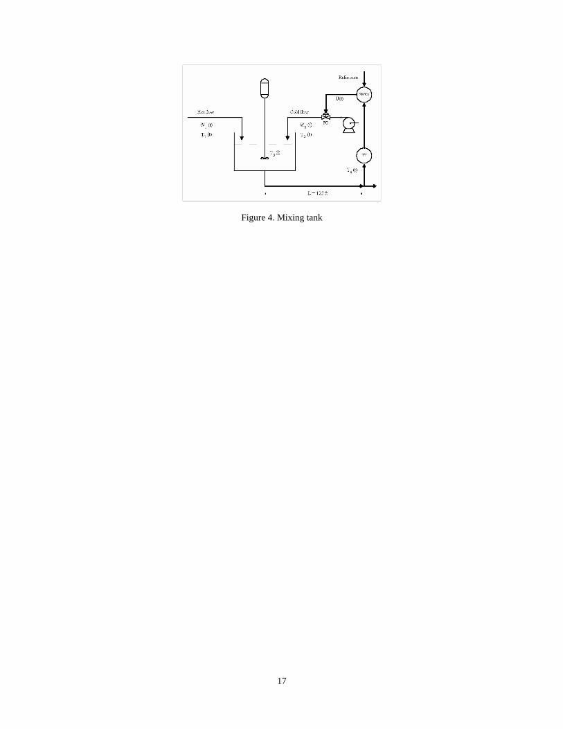
Figure 4. Mixing tank

17

0 100 200 300 400 500 600100

120

140

160

180

200

220

240

260

280

300

F l

o w

, l b

/m i

n

t i m e, m i n

0 100 200 300 400 500 600140

142

144

146

148

150

152

154

156

158

160

T, d

e g

F

t i m e, m i n

P I D

0 100 200 300 400 500 600140

142

144

146

148

150

152

154

156

158

160

T, d

e g

F

t i m e, m i n

S M Cr

Figure 5. Temperature response under SMCr and PID controller

18

Figure 6. Scheme of Continuous Stirred Tank Reactor

19

Figure 7. Process reaction curve for reactor

20

Figure 8. System responses for 10% in inlet flow

21

Figure 9. Effect of modeling error.

22

Figure 10. System responses for 10% change in inlet flow

for -10% error in modeling

23

Figure 11. System responses for 10% change in inlet flow

for 100% error in modeling

24