Embed Size (px)
Citation preview

SLIDING MODE CONTROL OF LINEARLY ACTUATED NONLINEAR SYSTEMS
BURAK DURMAZ
JUNE 2009

SLIDING MODE CONTROL OF LINEARLY ACTUATED NONLINEAR SYSTEMS
A THESIS SUBMITTED TO THE GRADUATE SCHOOL OF NATURAL AND APPLIED SCIENCES
OF MIDDLE EAST TECHNICAL UNIVERSITY
BY
BURAK DURMAZ
IN PARTIAL FULFILLMENT OF THE REQUIREMENTS FOR
THE DEGREE OF MASTER OF SCIENCE IN
MECHANICAL ENGINEERING
JUNE 2009

Approval of the thesis:
SLIDING MODE CONTROL OF LINEARLY ACTUATED NONLINEAR SYSTEMS
submitted by BURAK DURMAZ in partial fulfilment of the requirements for
the degree of Master of Science in Mechanical Engineering Department,
Middle East Technical University by,
Prof. Dr. Canan Özgen --------------------- Dean, Graduate School of Natural and Applied Sciences Prof. Dr. Suha Oral --------------------- Head of Department, Mechanical Engineering Prof. Dr. M. Kemal Özgören --------------------- Supervisor, Mechanical Engineering Dept., METU Assoc. Prof. Dr. Metin U. Salamcı --------------------- Co-Supervisor, Mechanical Engineering Dept., Gazi University
Examining Committee Members:
Prof. Dr. Y. Samim Ünlüsoy --------------------- Mechanical Engineering Dept., METU Prof. Dr. M. Kemal Özgören --------------------- Supervisor, Mechanical Engineering Dept., METU Prof. Dr. Bülent E. Platin --------------------- Mechanical Engineering Dept., METU Prof. Dr. Yücel Ercan --------------------- Mechanical Engineering Dept., TOBB ETU Assoc. Prof. Dr. Metin U. Salamcı --------------------- Mechanical Engineering Dept., Gazi University
Date: 04 June 2009
i
I hereby declare that all information in this document has been obtained and presented in accordance with academic rules and ethical conduct. I also declare that, as required by these rules and conduct, I have fully cited and referenced all material and results that are not original to this work.
Name, Last name: Burak DURMAZ
Signature :

ABSTRACT
SLIDING MODE CONTROL OF LINEARLY ACTUATED NONLINEAR SYSTEMS
Durmaz, Burak
Ms.C., Department of Mechanical Engineering
Supervisor : Prof. Dr. M. Kemal Özgören
Co-Supervisor : Assoc. Prof. Dr. Metin U. Salamcı
June 2009, 123 pages
This study covers the sliding mode control design for a class of nonlinear
systems, where the control input affects the state of the system linearly as
described by . The main streamline of the study is
the sliding surface design for the system. Since there is no systematic way of
designing sliding surfaces for nonlinear systems, a moving sliding surface is
designed such that its parameters are determined in an adaptive manner to cope
with the nonlinearities of the system. This adaptive manner includes only the
automatic adaptation of the sliding surface by determining its parameters by
means of solving the State Dependent Riccati Equations (SDRE) online during
the control process. The two methods developed in this study: SDRE combined
sliding control and the pure SDRE with bias terms are applied to a longitudinal
model of a generic hypersonic air vehicle to compare the results.
( ) ( ) ( )= + +x A x x B x u d x&
ii

iii
Keywords: Sliding Mode Control, Variable Structure Control Systems (VSCS),
State Dependent Riccati Equations (SDRE), Adaptive Control

ÖZ
DOĞRUSAL EYLETİMLİ DOĞRUSAL OLMAYAN SİSTEMLERİN KAYAN KİPLİ KONTROLU
Durmaz, Burak
Yüksek Lisans, Makina Mühendisliği Bölümü
Tez Yöneticisi : Prof. Dr. M. Kemal Özgören
Ortak Tez Yöneticisi: Doç. Dr. Metin U. Salamcı
Haziran 2009, 123 sayfa
Bu çalışma, durum değişkenleri kontrol girdilerince doğrusal olarak etkilenen
doğrusal olmayan sistemler için kayan kipli kontrolcu tasarımını
kapsamaktadır. Böyle bir sistem, ( ) ( ) ( )= + +x A x x B x u d x& biçiminde
tanımlanabilir. Çalışmanın ana hattını, sistem için kayma yüzeyinin
tasarlanması oluşturmaktadır. Doğrusal olmayan sistemler için sistematik bir
kayma yüzeyi tasarlama yöntemi bulunmadığından bu çalışmada hareketli
fakat parametreleri sistemin doğrusal olmayan özelliklerini etkisizleştirmek
üzere sürekli uyarlanan bir kayma yüzeyi tasarlanmıştır. Buradaki uyarlama
biçimi, kayma yüzeyi parametrelerinin Durum Bağımlı Riccati
Denklemleri’nin (DBRD) kontrol süreci sırasında an be an çözülerek
hesaplanmasını ve bu hesaplamalar kullanılarak yüzeyin otomatik olarak
uyarlanmasını kapsamaktadır. Bu çalışmada geliştirilen iki yöntem: DBRD ile
birleştirilmiş kayan kipli kontrolcü ve bias terimler içeren DBRD kontrol
tasarımı hipersonik bir hava aracının boylamsal modeline uygulanmıştır.
iv

v
Anahtar Kelimeler: Kayan Kipli Kontrol, Değişken Yapılı Kontrol Sistemleri,
Durum Bağımlı Riccati Denklemleri, Uyarlamalı Kontrol.

vi
To My Family
vii
ACKNOWLEDGMENTS
The author wishes to express his deepest gratitude to his supervisor Prof. Dr.
M. Kemal Özgören and co-supervisor Assoc. Prof. Dr. Metin U. Salamcı for
their guidance, advice, criticism, encouragements and insight throughout the
research.
The author also owes special thanks to his friend G. Serdar Tombul for his
contributions and to his engineering leader in the company Burcu Özgör
Demirkaya for her support and tolerance.
As a last word, the author is grateful to his family for their understanding,
devotion and for the opportunities they provided.

viii
TABLE OF CONTENTS
ABSTRACT........................................................................................................ii ÖZ.......................................................................................................................iv ACKNOWLEDGMENTS.................................................................................vii TABLE OF CONTENTS.................................................................................viii LIST OF FIGURES............................................................................................xi LIST OF SYMBOLS.......................................................................................xiv CHAPTER 1. INTRODUCTION.......................................................................................1
1.1 Sliding Mode Control........................................................................1
1.2 Literature Survey...............................................................................4 1.3 Scope of the Thesis Study.................................................................7
2. THEORATICAL BACKGROUND............................................................9
2.1 Introduction to SMC Design Technique............................................9
2.1.1 Sliding Surfaces...........................................................................9
ix
2.1.2 Controller Design......................................................................15
2.1.3 Summary....................................................................................20
2.2 Methodology Used in This Study....................................................22
2.2.1 SMC Combined with SDRE (Adaptive Sliding Mode
Control) .....................................................................................25
2.2.2 Pure SDRE Method...................................................................48
3. APPLICATION OF THE DESIGNED CONTROLLER TO A HYPERSONIC AIR VEHICLE MODEL.........................................................52
3.1 Mathematical Model of a Hypersonic Air Vehicle..........................53
3.1.1 Nomenclature.............................................................................53
3.1.2 Differential Equations of the System.........................................55
3.2 Sliding Mode Control Design for the Hypersonic Air Vehicle Model...............................................................................................58
3.3 Computer Simulations for the Designed Controller........................71
3.3.1 Simulations for the Case 1: Without Disturbance.....................75
3.3.2 Simulations for the Case 2: With Disturbance..........................84
4. CONCLUSIONS...........................................................................................97
4.1 Summary..........................................................................................97
4.2 Major Conclusions...........................................................................98 4.3 Recommendations for Future Work..............................................101

x
REFERENCES................................................................................................102 APPENDICES.................................................................................................107 APPENDIX A MAIN SCRIPT....................................................................107 APPENDIX B FUNCTION FOR DESIGNING CONTROLLER..............111 APPENDIX C FUNCTION FOR CONSTRUCTING SYSTEM AND CONTROL MATRICES...........................................115 APPENDIX D FUNCTION FOR TRANSFORMING THE SYSTEM TO CANONICAL FORM.........................................................118 APPENDIX E FUNCTION FOR SLIDING SURFACE SLOPE DETERMINATION............................................................120 APPENDIX F BRIEF USER MANUAL.....................................................122 VITA...............................................................................................................123

LIST OF FIGURES FIGURES Figure 2.1 Graphical interpretation of equations (2.2) and (2.4) (n=2).............13 Figure 2.2 Effect of K on the Chattering Phenomenon....................................39 Figure 2.3 Typical SMC Input..........................................................................40 Figure 3.1 Free Body Diagram of a Simplified Hypersonic Air Vehicle..........55 Figure 3.2 Velocity Change...............................................................................76 Figure 3.3 Flight Path Angle.............................................................................76 Figure 3.4 Altitude Change...............................................................................77 Figure 3.5 Angle of Attack................................................................................77 Figure 3.6 Pitch Rate.........................................................................................78 Figure 3.7 Elevator Deflection..........................................................................78 Figure 3.8 Throttle Setting................................................................................79 Figure 3.9 Variation of the Sigma Function – Deviation from Sliding Surface.............................................................................................79 Figure 3.10 First and Second Sliding Surface Offset........................................80 Figure 3.11 First and Second Components of the Sliding Surface Slope...............................................................................................80 Figure 3.12 Third and Fourth Components of the Sliding Surface Slope...............................................................................................81
xi

xii
Figure 3.13 Fifth and Sixth Components of the Sliding Surface Slope...............................................................................................81 Figure 3.14 First and Second Components of the Disturbance.........................82 Figure 3.15 Third and Fourth Components of the Disturbance.........................82 Figure 3.16 Fifth Component of the Disturbance and Delta Angle of Attack.............................................................................................83 Figure 3.17 Velocity Change.............................................................................85 Figure 3.18 Flight Path Angle...........................................................................85 Figure 3.19 Altitude Change.............................................................................86 Figure 3.20 Angle of Attack..............................................................................86 Figure 3.21 Pitch Rate.......................................................................................87 Figure 3.22 Elevator Deflection........................................................................87 Figure 3.23 Throttle Setting..............................................................................88 Figure 3.24 Variation of the Sigma Function – Deviation from the Sliding Surface............................................................................................88 Figure 3.25 First and Second Sliding Surface Offset........................................89 Figure 3.26 First and Second Components of the Sliding Surface Slope Slope...............................................................................................89 Figure 3.27 Third and Fourth Components of the Sliding Surface Slope...............................................................................................90 Figure 3.28 Fifth and Sixth Components of the Sliding Surface Slope...............................................................................................90 Figure 3.29 First and Second Components of the Transformed Disturbance.....................................................................................91 Figure 3.30 Third and Fourth Components of the Transformed Disturbance.....................................................................................91

xiii
Figure 3.31 Fifth Component of the Transformed Disturbance and Delta Angle of Attack........................................................................................92 Figure 3.32 Control Inputs for Integration Time Step is 0.1.............................94 Figure 3.33 Control Inputs for Integration Time Step is 0.01...........................95 Figure 3.34 Control Inputs for Integration Time Step is 0.001.........................95 Figure 3.35 Control Inputs for Integration Time Step is 0.5.............................96

LIST OF SYMBOLS
A Speed of Sound
DC Drag Coefficient
LC Lift Coefficient
( )MC q Moment Coefficient due to Pitch Rate
( )MC α Moment Coefficient due to Angle of Attack
( )M eC δ Moment Coefficient due to Elevator Deflection
TC Thrust Coefficient
C Reference Length
D Drag
h Altitude
yyI Moment of Inertia
L Lift
M Mach Number
yyM Pitching Moment
m Mass
q Pitch Rate
ER Radius of the Earth
r Radial Distance from Earth’s Center
S R
eference Area
T Thrust
xiv

V Velocity
α Angle of Attack
β Throttle Setting
γ Flight-Path Angle
eδ Elevator Deflection
μ Gravitational Constant
ρ Density of Air
ASMC
Adaptive Sliding Mode Control
LQR Linear Quadratic Regulator
SMC
Sliding Mode Control
SDRE State Dependent Riccati Equation
xv

1
CHAPTER 1
INTRODUCTION
1.1 Sliding Mode Control
Variable Structure Control Systems (VSCS) evolved from the pioneering work
of Emel’yanov and Barbashin in the early 1960s in Russia. The ideas did not
appear outside of Russia until the mid 1970s when a book by Itkis and a survey
paper by Utkin [1] are published in English. VSCS concepts have subsequently
been utilised in the design of robust regulators, model-reference systems,
adaptive schemes, tracking systems, state observers and fault detection
schemes. The ideas have successfully been applied to problems as diverse as
automatic flight control, control of electric motors, chemical processes,
helicopter stability augmentation systems, space systems and robots. [2]
VSCS, as the name suggests, are a class of systems whereby the ‘control law’
is deliberately changed during the control process according to some defined
rules which depend on the state of the system. Based on the concept of VSCS,
the aim is to design a controller which will be sought to force the system states
to reach, and subsequently remain on, a predefined surface within the state
space.

2
The state space behaviour of the system is described as an ideal sliding motion
when its state is confined to the surface. The advantages of obtaining such a
motion are twofold: firstly, there is a reduction in the order of the dynamics
which simplifies the controller design; secondly the sliding motion is
insensitive to the matched uncertainties, which are the parameter variations
and/or unknown inputs that occur in the same channels with the control inputs.
This insensitivity at least against the matched uncertainties makes the
methodology an attractive one for designing robust controllers for uncertain
systems.
Model imprecision may come from actual uncertainty about the plant (e.g.,
unknown plant parameters), or from the purposeful choice of a simplified
representation of the system’s dynamics. Modelling inaccuracies can be
classified into two major kinds: structured (or parametric) uncertainties and
unstructured uncertainties (or unmodelled dynamics). The first kind
corresponds to inaccuracies in the terms actually included in the model, while
the second kind corresponds to the neglected higher order terms in the dynamic
model.
Modelling inaccuracies can have strong adverse effects on nonlinear control
systems. One of the most important approaches to dealing with model
uncertainty is robust control. The typical structure of a robust controller is
composed of a nominal part, similar to an ordinary feedback control law, and
additional terms aimed at dealing with model uncertainty. Sliding Mode
Control (SMC) technique is one of the important robust control approaches.
For the class of systems to which it applies, SMC design provides a systematic
approach to the problem of maintaining stability and consistent performance in
the face of modelling imprecision.

3
Many different techniques have been developed for years to design sliding
mode controllers. But the baselines of all different design techniques are very
similar and consist of two main steps:
• Design the sliding (switching) surface in the state space so that the
reduced-order sliding motion satisfies the specifications imposed by the
designer,
• Determine the control law such that the trajectories of the closed-loop
motion are directed towards the sliding surface and tried to be kept on
the surface thereafter.
Discontinuity occurs due to the difference between the out-of-surface and
surface-bound control laws. It can be avoided by replacing the sudden
discontinuous switching between the two control laws with a rapid but
continuous and gradual transition, such as using some kind of a saturation
function instead of the sign function.

4
1.2 Literature Survey
As mentioned in Chapter 1.1, SMC design techniques are mainly developed
after 1970s. Then, many studies have been done for the use of SMC technique
both for linear and non-linear systems. Basically, research on SMC has
recently developed in two main areas. The first is static SMC based on the
works of DeCarlo et al. [3], Utkin [4] and Luk’yanov and Dodds [5]. The
second approach is dynamic SMC which is based on differential (input-output)
I-O systems, one of which is the work of Sira-Ramirez [6].
SMC is generally robust with respect to some kinds of uncertainties and
modelling inaccuracies. For linear systems, the robustness property is well
established. Robustness results also exist for particular types of non-linear
systems. A general framework for the design of nonlinear sliding mode
controllers based on the action of a one-parameter subgroup of
diffeomorphisms on the sliding surface is represented in [7].
In most SMC schemes, the control laws usually utilise full-state feedback. In
practice, this is not always possible, since the system states are not available or
are expensive to measure. In case of so called immeasurable states, observer-
based sliding mode controllers have been designed as studied in [8] by means
of constructing an observer to estimate the unavailable states and then
synthesising a SMC law based on the estimated states.
In addition to this, chattering phenomenon takes much more attraction in recent
studies since it is thought that chattering is the only remaining obstacle in SMC
design technique. Many design methods are proposed to overcome the effects
of chattering.

5
There are many review papers on SMC. A recent one is prepared by K. David
Young, Vadim I. Utkin and Ümit Özgüner in 1999 [9] which is a guide to
summarise the basic design solutions and emphasise the effect of chattering
phenomenon.
One of the recent trends on the SMC research is to combine the other control
system design techniques with SMC. Within this context, the addition of
adaptation capability to classical SMC may be considered as the combination
of adaptive control and SMC. Furthermore, the addition of adaptation
capability, named after as “Adaptive Sliding Mode Control (ASMC)”, makes
the sliding more sensible if it is thought that SMC is a subset of VSCS.
Some studies, which have been addressing the problem of designing adaptive
sliding mode controllers for specific systems, can be found in the literature. In
[10], adaptive sliding mode controller is designed for a hypersonic air vehicle
model. In the study, firstly, the non-linear model of the hypersonic air vehicle
is linearised by the application of input-output linearisation method. After that,
two decoupled sliding surfaces are chosen based on the error dynamics. Errors
are defined as the difference between the current velocity, altitude and the
steady state (desired) values of the velocity and altitude respectively. Lastly,
the sliding control design is accomplished by choosing control inputs such that
the sliding conditions imply that the distance to the sliding surface decreases
along all system trajectories are satisfied. Furthermore, the sliding condition
makes the sliding surface an invariant set, i.e., once the system trajectories
reach the surface, it will remain on it for the rest of the time. In addition, for
any initial condition, the sliding surface is reached in a finite time.

6
In the work of Xu, H., et al [10], the sliding mode controller is combined with
an on-line parameter estimator forming an adaptive sliding mode controller as
well. The adaptive laws used to adapt the parameter estimations have been
derived using the Lyapunov synthesis approach. The SMC alone and combined
with the addition of an adaptive law (ASMC) techniques are simulated then
accordingly under the presence of parametric uncertainty to see the advantages
of the second method over the first one. As expected, a significant
improvement in controller performance is observed. It is seen that the level of
the control effort in the adaptive case is significantly smaller.

7
1.3 Scope of the Thesis Study
The main contribution of this study can be considered to be the addition of an
adaptive manner to the SMC design for a state dependent and linearly actuated
non-linear system. This is a contribution to the area of ASMC (Adaptive SMC)
design, which is an attractive area for the researchers since it combines the
power of SMC against uncertainties and disturbances with the ability of
adapting the controller while the system is changing.
The technique used in [10] to design an ASMC for the hypersonic air vehicle
model is explained in section 1.2. In this study, on the other hand, a different
methodology has been developed to design the adaptive sliding mode
controller for the same model used in [10]. First of all, the system is not
linearised to design the sliding mode controller, in other words, the non-
linearity of the original system is kept during the controller design phase.
Secondly, the adaptation manner is added directly to SMC by means of
adapting the slope of the sliding surface as well as its offset from the origin of
the state space in accordance with the changes in the system state.
To make this adaptation, the so-called State Dependent Riccati Equations
(SDRE) are solved while the state variables of the system are changing. Then
the corresponding sliding surface slope and sliding surface offset are
determined based on these calculations.
This technique not only turns the sliding mode controller to an adaptive one but
it also allows to determine the slope and offset of the sliding surface optimally
depending on the specified weighting matrices of a selected performance
index.

8
The method can be outlined as follows (although a detailed explanation is
given in section 2.2);
The system (represented by the state space formulation) is divided into two
subsystems by using a state variable transformation such that all the control
inputs are collected in the second subsystem while there remains no control
input in the first subsystem, which is also called the reduced order system.
Considering the first subsystem, the sliding surface is defined as a hyper
surface in the state space based on two parameters: the sliding surface slope
and the sliding surface offset. In this work, these parameters are determined
optimally as functions of the state variables using the SDRE technique. The
second subsystem, on the other hand, is used to determine the control inputs.
The control inputs are determined to consist of two parts: the first part (known
as the nominal control) is responsible of keeping the system state on the sliding
surface and the second part (known as the switching control) is responsible of
driving the system state toward the sliding surface whenever it is away from it.

9
CHAPTER 2
THEORETICAL BACKGROUND
2.1 Introduction to SMC Design Technique
Following three sections are mainly tailored from [11] to give brief information
about the two main steps of the sliding mode control design.
2.1.1 Sliding Surfaces
This section analyses the Variable Structure Control (VSC) as a high-speed
switched feedback control leading up to a sliding mode. For instance, each
feedback path gains are switched between two values according to a rule that
depends on the value of the system state at each instant. The purpose of the
switching control law is to drive the state trajectory of the system onto a pre-
specified (user-chosen) surface in the state space and to maintain the state
trajectory on this surface for the subsequent time interval. This surface is called
a switching surface. When the state trajectory is “above” the surface, the
feedback controller uses one gain and a different gain if the state trajectory is
“below” the surface. This surface defines the rule for a proper switching. This
surface is also called a sliding surface (sliding manifold). [16]

Ideally, once intercepted, the switched control maintains the state trajectory on
the surface forever and the state of the system slides on the surface toward the
stable equilibrium point. The most important part is to design a switched
control that drives the system state to the switching surface and keep it on the
surface upon interception. A Lyapunov approach is used to carry out this task.
The Lyapunov method is usually used to determine the stability properties of
an equilibrium point without solving the state equation. Let be a
continuously differentiable scalar function defined in a domain D that contains
the origin. A function is said to be positive definite if V and
for
( )V x
(0) = 0(x)V
(x) > 0V 0≠x . It is said to be negative definite if and
for
(0) = 0V (xV ) < 0
0≠x . The Lyapunov method is to assure that the derivative of a properly
defined positive definite function of the system state is negative definite. The
function has a negative value when the function itself has a positive value and
vice versa. Thus, the stability of the system is assured about the origin of the
state space.
Lyapunov method, which was explained briefly above, is used to design the
sliding mode controller. A candidate Lyapunov function, that characterises the
motion of the system state to the sliding surface, is defined. For each chosen
switched control structure, the “gains” are chosen such that the derivative of
this Lyapunov function is negative definite, thus ensuring motion of the system
state to the surface. After appropriate design of the sliding surface, a switched
controller is designed so that the system state trajectories point towards the
surface such that the state is driven to the this surface. Once system states reach
to the sliding surface, they remain on it. This kind of controllers results in
discontinuous closed-loop systems. [16]
10
The main concepts and notations of sliding mode control are presented first for
systems with a single control input, which allow us to develop intuition about
the basic aspects.
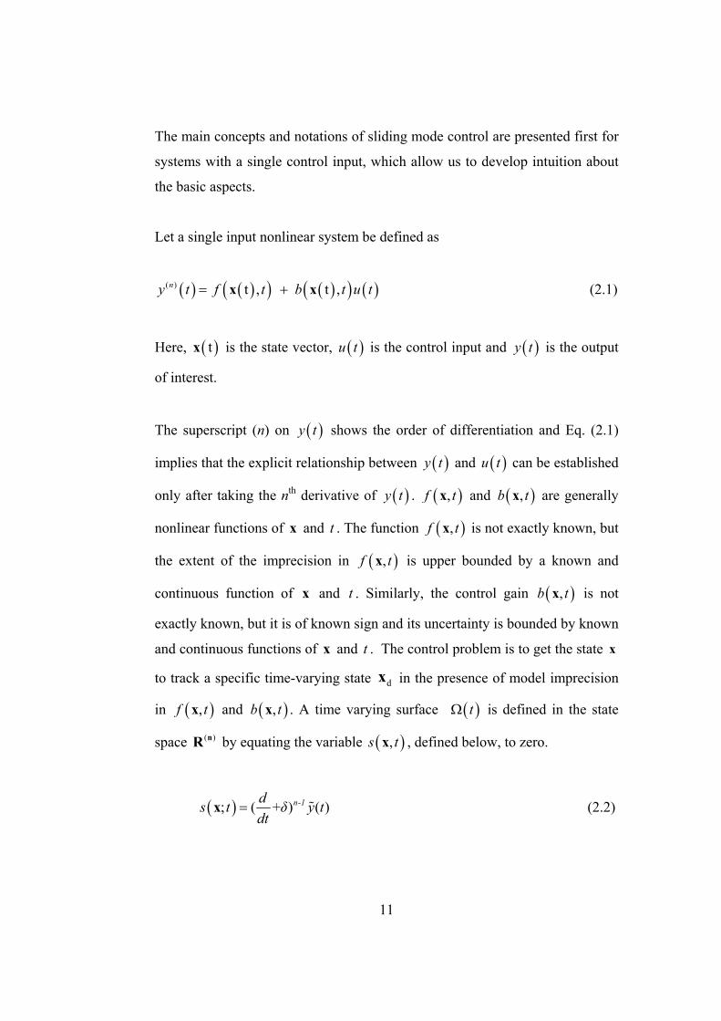
Let a single input nonlinear system be defined as
( ) ( )( ) ( )( ) ( )( ) t , t ,ny t f t b t u t= +x x (2.1)
Here, is the state vector, ( )tx ( )u t is the control input and is the output
of interest.
( )y t
The superscript (n) on ( )y t shows the order of differentiation and Eq. (2.1)
implies that the explicit relationship between ( )y t and ( )u t can be established
only after taking the nth derivative of ( )y t . ( ),f tx and ( ), txb are generally
nonlinear functions of x and . The function t ( ),f tx is not exactly known, but
the extent of the imprecision in ( ),f t
dx
x is upper bounded by a known and
continuous function of and t . Similarly, the control gain is not
exactly known, but it is of known sign and its uncertainty is bounded by known
and continuous functions of and t . The control problem is to get the state
to track a specific time-varying state in the presence of model imprecision
in
x ( ,b tx )
)
x x
( ,f tx and . A time varying surface ( ,b x )t ( )tΩ is defined in the state
space by equating the variable ( )nR ( ),s tx , defined below, to zero.
( ); ( + ) (n-1ds t δ y tdt
=x % ) (2.2)
11
Here, δ is a strictly positive constant, ( ) ( ) ( )d
y t y t y t= −%
d (x
and
. The problem of tracking the n-dimensional vector can
in effect be replaced by a stabilisation problem in .
d( ) ( )x x x% ( )t t= − t )t
s
The sliding surface is defined by Ω ( , ) 0s t =x
1)n-
and the system’s behaviour on
the surface is called sliding mode or sliding regime. From (2.2) it is seen
that the expression of contains
Ω
s (y% . So, by differentiating only once, the
input u to appears for the subsequent manipulations.
s
Furthermore, the bounds on can be directly translated into bounds on the
tracking error vector x , and therefore the scalar represents a true measure of
the tracking performance. The corresponding transformations of performance
measures assuming
s
%
(0y
s
) 0=% is:
( )0, ( ) 0, ( ) (2 )
0,......, -1
i it s t t y t
i n
φ δ ε∀ ≥ ≤ ⇒ ∀ ≥ ≤
=
% (2.3)
where 1/ n-ε φ δ= . In this way, an nth order tracking problem can be replaced
by a 1st order stabilisation problem. The simplified, 1st order problem of
keeping the scalar at zero can now be achieved by choosing the control law
of (2.1) such that outside of
s
u ( )tΩ
21 -2
d s sdt
η≤ (2.4)
where η is a strictly positive constant.
12
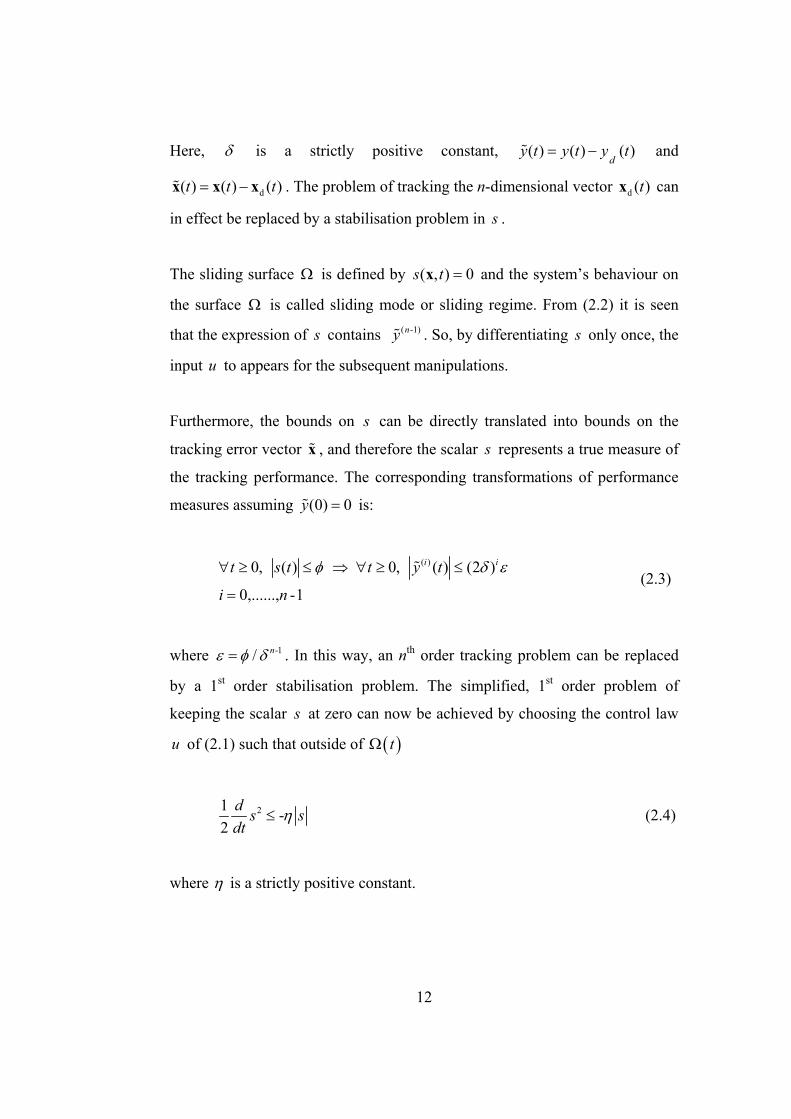
Condition (2.4) states that the squared “distance” to the surface, as measured
by , decreases along all the system trajectories. 2s
Thus, it constrains trajectories to point towards the surface . In particular,
once on the surface, the system trajectories remain on the surface. In other
words, satisfying the sliding condition makes the surface an invariant set (a set
for which any trajectory starting from an initial condition within the set
remains in the set for all times). Furthermore (2.4) also implies that some
disturbances or dynamic uncertainties can be tolerated while still keeping the
surface an invariant set.
( )tΩ
Figure 2.1 Graphical interpretation of equations (2.2) and (2.4) (n=2) (Resource: Slotine and Li 1991, [11])
13

Finally, satisfying (2.4) guarantees that if condition ( ) (d 0 0=x x ) is not exactly
verified, i.e., if is actually off ( = 0)tx ( )d = 0tx , the surface will be
reached in a finite time smaller than
( )tΩ
( = 0) /s t η . Assume for instance that
, and let be the time required to hit the surface . ( ) = 0 0ts > reacht 0s =
Integrating (2.4) between t = 0 and leads to reacht
0 ( = 0) = ( = ) ( = 0) ( 0)reach reachs t s t t s t tη− − ≤ − − (2.5)
which implies that
( = 0) / reach t s t η≤ (2.6)
The similar result starting with ( )= 0 < 0s t can be obtained as
( = 0) / reach t s t η≤ (2.7)
For initial condition, the state trajectory reaches the sliding surface in a finite
time smaller than ( = 0) / s t η , and then slides on the surface towards ( )d tx
exponentially, with a time-constant equal to 1 λ .
In summary, the idea is to use a well-behaved function of the tracking error, ,
according to (2.2), and then select the feedback control law in (2.1) such that
remains a Lyapunov-like function of the closed-loop system, despite the
presence of model imprecision and of disturbances.
s
u2s
14

2.1.2 Controller Design
The controller design procedure consists of two steps. First, one selects the
feedback control law u as to verify sliding condition (2.4). However, the
control law has to be discontinuous across ( )tΩ in order to cope with the
modelling imprecision and the disturbances. It is inapplicable to implement the
associated control switching, since this result with chattering. Chattering is
undesirable in practice, since it involves high control activity and may excite
high frequency dynamics neglected in the course of modelling. Therefore, in
the second step, an optimal trade-off between control bandwidth and tracking
precision is accomplished by means of smoothing the discontinuous control
law u in a suitable manner. [16]
As an example, consider a simple second order system described by
( ) = ( ) ( )x t f x,t u t + && (2.8)
where ( )f x,t
( )
is generally nonlinear and/or time/state varying and is estimated
as f x,t ( )u t , is the control input, and ( )x t is the state to be controlled so that
it follows a desired trajectory ( )dx t . The estimation error in ( )f x,t is
assumed to be bounded by some known function , so that = ( )F F x,t
ˆ ( ) ( ) ( )f x,t f x,t F x,t− ≤ (2.9)
Let the distance to the sliding surface be defined according to (2.2). That is,
15

( ) = + ( ) = ( ) + ( )ds t x t x t x tdt
γ γ⎛ ⎞⎜ ⎟⎝ ⎠
&% % % (2.10)
Differentiation of yields ( )s t
( ) = ( ) ( ) + ( )ds t x t x t x tγ− && && && % (2.11)
Substituting Equation (2.8) in Equation (2.11), becomes, ( )s t&
( )( ) = ( )+ ( ) + γ ( )ds t f x,t u t x t x t− && && % (2.12)
The approximate control ( )u t to achieve is ( ) = 0s t&
( ) ˆˆ = ( ) ( ) ( ) du t x t x t f x, tγ− −&&& % (2.13)
( )ˆ u t is the nominal control or the sliding-phase control, which would keep
the system state on the sliding surface if ( )f x,t and ˆ ( ) f x, t were equal.
On the other hand, if ( ) 0s t ≠ , i.e. if the system state is not on the sliding
surface, it can be forced to be zero according to the following condition
deduced from the Lyapunov's second stability theorem.
21 ( ( )) ( ) ( ) ( )2
d s t s t s t s tdt
η= ≤ −& (2.14)
This condition can be satisfied by the following control input,
16

( ) ( ) ( ) ( )ˆ = sgn s tu t u t k x,t ⎡ ⎤− ⎣ ⎦ (2.15)
With this control, Inequality (2.14) becomes
ˆ( )[ ( , ) ( ) ( , )sgn( ( )) ( )] ( )ds t f x t u t k x t s t x x t s tγ η+ − − + ≤ −&&& % (2.16)
Let Eq. (2.13) be substituted. Then,
ˆ( )[ ( , ) ( , )] [ ( , ) ] ( )s t f x t f x t k x t s tη− ≤ − (2.17)
In the worst case,
ˆ( , ) ( , ) ( , )sgn[ ( )]f x t f x t F x t s t− = (2.18)
Then,
[ ( , ) ( , )] ( ) 0k x t F x t s tη− − ≥ (2.19)
Hence, by choosing large enough, such as ( , )k x t
( ) ( ), ,k x t F x t η> + (2.20)
the satisfaction of condition (2.14) can be ensured.
The preceding simple example shows the main advantages of transforming the
original tracking problem into a simple 1st order stabilisation problem for the
variable s.
17

In the first-order systems, the intuitive feedback control strategy “if the error is
negative, push on to the positive direction; if the error is positive, push on to
the negative direction” works. The same statement is not true in a general
higher-order system.
Now consider the second order system described by,
( ) = ( ) + ( ) ( )x t f x, t b x,t u t&& (2.21)
where is bounded as ( )b x,t
( ) ( ) ( )0 < < < maxminb x,t b x,t b x,t (2.22)
The control gain and its bound can be time varying or state dependent.
Since the control input enters multiplicatively in the dynamics, the geometric
mean of the lower and upper bound of the gain is a reasonable estimate:
(b x,t)
( ) ( ) ( )ˆ = min maxb x,t b x,t b x,t (2.23)
Bounds can then be written in the form
ˆ-1 b
bβ β≤ ≤ (2.24)
where ( )1/2max min/ b bβ =
Since the control law will be designed to be robust to the bounded
multiplicative uncertainty, β is called the margin of the design.
18

It can be proved that the control law
( ) ( ) ( ) ( ) ( ){ }1ˆ ˆ = x,t [ sgn ]u t b u t k x,t s t− − (2.25)
with
( ) ( ) ( ) ( ) ( )ˆ ( + ) + 1 k x,t x,t F x,t x,t u tβ η β≥ ⎡ ⎤⎣ ⎦− (2.26)
satisfies the condition (2.14), or sliding condition.
The control law for a higher order system can be derived based on a similar
approach.
19
20
2.1.3 Summary
By courtesy of its robustness properties, sliding mode controller provides good
performance for the following two cases which can be defined as two major
design difficulties encountered in the design of a control algorithm:
1. The system is nonlinear with time-varying parameters and uncertainties;
2. The performance of the system depends strongly on the knowledge of the
disturbances;
For the class of systems to which it applies, sliding mode controller design
provides a systematic approach to the problem of maintaining stability and
consistent performance in the face of modelling imprecision. The main
advantage of sliding mode control is that the system’s response remains
insensitive to some kinds of model uncertainties and disturbances.
A generic hypersonic air vehicle model is used in this thesis as a case study
example to observe the performance of the proposed sliding mode controller.
The problem can be summarised as to design a nonlinear and time-varying
control system for tracking velocity and altitude commands under the presence
of disturbance for this hypersonic air vehicle. Hypersonic air vehicles are
sensitive to changes in flight condition as well as physical and aerodynamic
parameters due to their design and flight conditions of high altitudes and Mach
numbers. For example, at cruise flight at an altitude of 110,000 ft and Mach 15,
a 1-deg increase in the angle of attack produces a relatively large load factor.
Furthermore, it is difficult to measure or estimate the atmospheric properties
and aerodynamic characteristics at high flight altitudes.

21
As a result; modelling inaccuracies can result and can have strong adverse
effects on the performance of the air vehicle’s control systems. Therefore,
employing a kind of robust control has been the main technique used for
hypersonic flight control. [10]
The sliding mode control, which is one of the most important robust control
techniques, provides a systematic approach to the problem of maintaining
stability and consistent performance in the face of modelling imprecision. The
main advantage of sliding mode control is that the system’s response remains
insensitive to model uncertainties and disturbances. On the other hand, the
sliding mode control requires a trade-off between robustness properties against
model uncertainties and disturbances and control system performances. It is
meant that the sliding mode control has drawbacks like large control effort
necessity and chattering in the face of model uncertainties and disturbances.
The performance of the sliding mode controller can be increased and these
drawbacks can be eliminated by combining the sliding mode controller with an
adaptive scheme. [10]

2.2 SMC Design Methodology Used in This Study
SMC design for nonlinear systems has been studied by various researchers [3,
7, 11, 18, 23]. It is well-known that there is no straight forward method to
design sliding surface for nonlinear systems since ensuring the stability of
sliding motion requires special assessment for the nonlinear system under
consideration. Therefore, sliding surface design for nonlinear systems is still an
active research field in SMC theory.
In this thesis, a relatively systematic method is proposed to design sliding
surface for nonlinear systems given by the following expression.
( ) ( )= +x A x x B x u& (2.27)
where and are the state and control vectors and n∈ℜx m∈ℜu ( ) n n×∈ℜA x
and are nonlinear State Dependent Coefficient (SDC) matrices.
Equation (2.27) is a special representation of the nonlinear dynamics described
by the following equation,
( )∈ℜB x n m×
( ) ( )= +x a x B x u& (2.28)
where and is obtained by using the so-called SDC
parameterisation [15].
( ) ( )=a x A x x ( )A x
The nonlinear dynamics given by (2.27) is studied by various authors in order
to design optimal controllers.
22

One of the recent approaches to the optimal controller design for the nonlinear
system is the so-called State Dependent Riccati Equations (SDRE) method [15,
28, 38, 39]. The basic idea in SDRE is to extend classical Linear Quadratic
Regulator (LQR) method to the nonlinear system equations. As seen in (2.27),
the nonlinear system equation is an extension of = +x Ax Bu& type Linear Time
Invariant (LTI) system which is well studied in terms of both optimal and state-
feedback controls in the literature. Therefore by extending the control theory
for LTI systems to (2.27), it may be possible to design similar type of
controllers for the nonlinear system.
One of the problems of SDRE based control design for nonlinear systems is to
ensure the system stability. Unfortunately, there are no global stability results
seen in the literature. Nevertheless, local asymptotical stability of SDRE based
optimal control for the nonlinear system given by (2.27) is proved by different
authors. For the sake of completeness, the local stability result of [15] is given
below without its proof.
Theorem 1
Assume that the SDC parameterisation is chosen such that col ( ){ } 1∈A x in
the neighbourhood about the origin that the pair Ω { }( ),A x ( )B x is pointwise
stabilisable in the linear sense for all ∈Ωx . Then the SDRE nonlinear
regulator produces a closed-loop solution which is locally asymptotically stable
[15].
Another problem in the SDRE based controller design is to accomplish the
SDC parameterisation since the parameterisation is not unique. However, one
of the most important factors in the parameterisation process is to assure the
pointwise controllability in the local region.
23

24
The details of SDRE theory and simulation results together with some real
applications can be found in [15, 28, 38, 39].
As can be seen in equation (2.27), there is no uncertain dynamics or
disturbance effects in the nonlinear expressions. Although it is possible to use
the idea of SDRE in order to design SMC for (2.27), the disturbance (or
modelling uncertainty) term is included into the nonlinear dynamics to
emphasise the disturbance rejection capability of the SMC. With this approach,
SMC is combined with SDRE which enables one to design SMC for a class of
nonlinear systems in a relatively systematic manner. Besides, by using State
Dependent parameters in sliding surface definition, the SMC can adapt the
controller against the nonlinearities and disturbances of the system which may
be regarded as an Adaptive Sliding Mode Control (ASMC). The method is
given in the following section.

2.2.1 SMC Combined with SDRE (Adaptive Sliding Mode Control)
The system to be controlled with this methodology is described as follows.
( ) ( ) ( )= + + +x A x x B x u f(x) d x& (2.29)
where and are the state and control vectors. Here, is
a nonlinear vector which includes the terms remained after SDC
parameterisation and/or the constant terms of the state dependent disturbance
vector. As for d(x), it is the state-dependent disturbance vector.
n∈ℜx m∈ℜu n∈ℜf(x)
SDRE control design method is based on freezing the nonlinear dynamics at
the given operating point and designing the controller at that operating point. In
other words, pointwise controller design is accomplished and control
parameters are updated at each operating point. Therefore, linear control design
techniques (which are updated at each operating point) can be used for the
nonlinear system.
SMC design for LTI systems are studied thoroughly in the literature (see [2]
and [4] for more details). In this study, the SMC design method for LTI
systems is used and is extended to the nonlinear dynamics. As in the case of
SDRE based controller design, the nonlinear system is frozen at each operating
point and pointwise SMC is designed for each LTI dynamics. In order to
design SMC for the LTI system, the system is transformed so that it can be
separated into two parts such that one of the parts is in the so-called reduced
order form in which the control inputs are absent. The transformed system is to
be represented by an equation such as,
25

26
z= + + +z z zz A z B u f d& (2.30)
where
11 12
21 22
z z
zz z
⎡ ⎤⎢ ⎥= ⎢ ⎥⎢ ⎥⎣ ⎦
A AA A A ,
21 21 2 2, , z
⎡ ⎤ ⎡ ⎤ ⎡= =
⎤=⎢ ⎥ ⎢ ⎥ ⎢ ⎥
⎣ ⎦ ⎣ ⎦ ⎣
1z 1zz z
z z
0 0 f dB F DB B f d ⎦
(2.31)
and [ ]2 21 2=B B B 2 is non-singular. In the expanded form, the equation
becomes,
11 121 1 1
21 22 21 21 2 22 2 2
+z z
z z
⎡ ⎤ ⎡ ⎤ ⎡ ⎤ ⎡⎡ ⎤ ⎡ ⎤ ⎡ ⎤⎢ ⎥= + +⎤
⎢ ⎥ ⎢ ⎥ ⎢⎢ ⎥ ⎢ ⎥ ⎢ ⎥⎢ ⎥⎣ ⎦ ⎣ ⎦ ⎣ ⎦⎥
⎣ ⎦ ⎣ ⎦ ⎣⎢ ⎥⎣ ⎦
1z 1z
z z
A A 0 0 f dz z uA A B B f dz z u
&
& ⎦ (2.32)
The required transformation described above can be achieved by the following
equation
=z Tx (2.33)
where is the new state vector and is the state transformation matrix which
is assumed to be non-singular.
z T
The state transformation matrix is not unique and there are different
methods to obtain it. One of the methods to find the transformation matrix is
the use of “QR decomposition” technique.
T

The QR decomposition (also called the QR factorisation) of a matrix is a
decomposition of the matrix into an orthonormal (or unitary) matrix Q and a right
triangular matrix R as indicated below.
A = QR (2.34)
There are several methods for finding the QR decomposition, such as by means
of the Gram–Schmidt process, Householder transformations, or Givens
rotations. Each has a number of advantages and disadvantages. In this study,
the special command of MATLAB, “qr” is used. It is used as described below.
[Tr : Temp] = qr(B)
Here Temp stands for a temporarily constructed matrix while Tr stands for the
matrix constructed for the transformation. This produces an upper triangular
matrix Temp of the same dimension as and a unitary matrix so that
= × Te . For sparse matrices, Tr is often nearly full. If is an
B Tr
B Tr mp B m n×
matrix, then Tr is m × m and Temp is m × n.
In the next step, Tr matrix is inverted first and its rows are re-ordered to reach
the final state transformation matrix T such that
z =B TB (2.35)
As a case study, consider the nonlinear dynamics of a hypersonic air vehicle
model which is used in Chapter 3. The state and control vectors are,
27
1
2
3
4
5
Vxxx hxx q
γ
α
⎡ ⎤⎡ ⎤⎢ ⎥⎢ ⎥⎢ ⎥⎢ ⎥⎢ ⎥⎢ ⎥= =⎢ ⎥⎢ ⎥⎢ ⎥⎢ ⎥⎢ ⎥⎢ ⎥⎣ ⎦ ⎣ ⎦
x
%%
%% and, (2.36)
1
2
euu
δβ
⎡ ⎤ ⎡ ⎤= =⎢ ⎥ ⎢ ⎥
⎣ ⎦⎣ ⎦u (2.37)
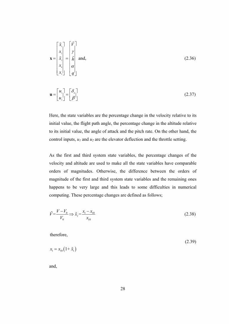
Here, the state variables are the percentage change in the velocity relative to its
initial value, the flight path angle, the percentage change in the altitude relative
to its initial value, the angle of attack and the pitch rate. On the other hand, the
control inputs, u1 and u2 are the elevator deflection and the throttle setting.
As the first and third system state variables, the percentage changes of the
velocity and altitude are used to make all the state variables have comparable
orders of magnitudes. Otherwise, the difference between the orders of
magnitude of the first and third system state variables and the remaining ones
happens to be very large and this leads to some difficulties in numerical
computing. These percentage changes are defined as follows;
0 1
0 1
= = 1V V x xV x
V x− −
⇒% % 10
0
(2.38)
( )1 10 1
therefore,
1 x x + x= %
(2.39)
and,
28

29
01 1 1x x x= && % (2.40)
0 33
0 3
= =h h x xh xh x− −
⇒% % 30
0
(2.41)
therefore,
( )3 30 31 x x x= + % (2.42)
and,
3 3 30x x x= && % (2.43)
where and 0V 10x are the initial values of the velocity and and 0h 30x are the
initial values of the altitude.
The term in (2.29) gets added to the system differential equation as a
result of the new definition of the first and third system state variables in the
form of percentages. This term is taken into account as a known disturbance
and it is compensated by the designed controller.
( )f x
The derivation of the state transformation matrix is shown below for the B
matrix used in the simulations of this study.
[ ] [ ]
12
22
5 5 5 2
42
51 52
000 0 x0
x x
bb
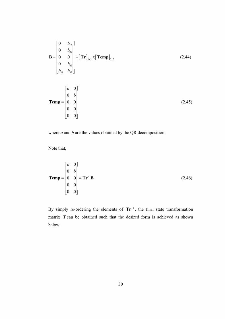
bb b
⎡ ⎤⎢ ⎥⎢ ⎥⎢ ⎥= =⎢ ⎥⎢ ⎥⎢ ⎥⎣ ⎦
B Tr Temp (2.44)
000 00 00 0
ab
⎡ ⎤⎢ ⎥⎢ ⎥⎢ ⎥=⎢ ⎥⎢ ⎥⎢ ⎥⎣ ⎦
Temp (2.45)
where a and b are the values obtained by the QR decomposition.
Note that,
1
000 00 00 0
ab
−
⎡ ⎤⎢ ⎥⎢ ⎥⎢ ⎥= =⎢ ⎥⎢ ⎥⎢ ⎥⎣ ⎦
Temp Tr B (2.46)
By simply re-ordering the elements of 1−Tr , the final state transformation
matrix can be obtained such that the desired form is achieved as shown
below,
T
30

z
0 00 00 0
00a
b
⎡ ⎤⎢ ⎥⎢ ⎥⎢ ⎥= = =⎢ ⎥⎢ ⎥⎢ ⎥⎣ ⎦
TB TB B (2.47)
In other words, this state transformation matrix is used to obtain the reduced
order forms of the system matrices , , and . The derivation of
these matrices is explained in the following part. By assuming a time varying
and/or a state dependent state transformation such as
zA zB zF zD
=z Tx (2.48)
and its derivative,
( )= + = + + = + + + +z Tx Tx TAx TBu Tx TA T x TBu Tf Td& & && & (2.49)
the new state equation is obtained as,
31
z
)
= + + +z z zz A z B u f d& (2.50)
Dimensions of the vector and matrix variables are given here to prevent any
misunderstanding.
n
m
nxm
∈ℜ
∈ℜ
∈ℜ
xuB
1
2
n
n m
m
−
∈ℜ
∈ℜ
∈ℜ
zz
z
( ) (
( )
2
11
12
m m
n m n mz
n m mz
×
− × −
− ×
∈ℜ
∈ℜ
∈ℜ
B
A
A
( )
( )
21
22
1
mx n mz
mxmz
n mz
−
−
∈ℜ
∈ℜ
∈ℜ
A
A
f
( )2
1
2
mz
n mz
mz
−
∈ℜ
∈ℜ
∈ℜ
f
d
d
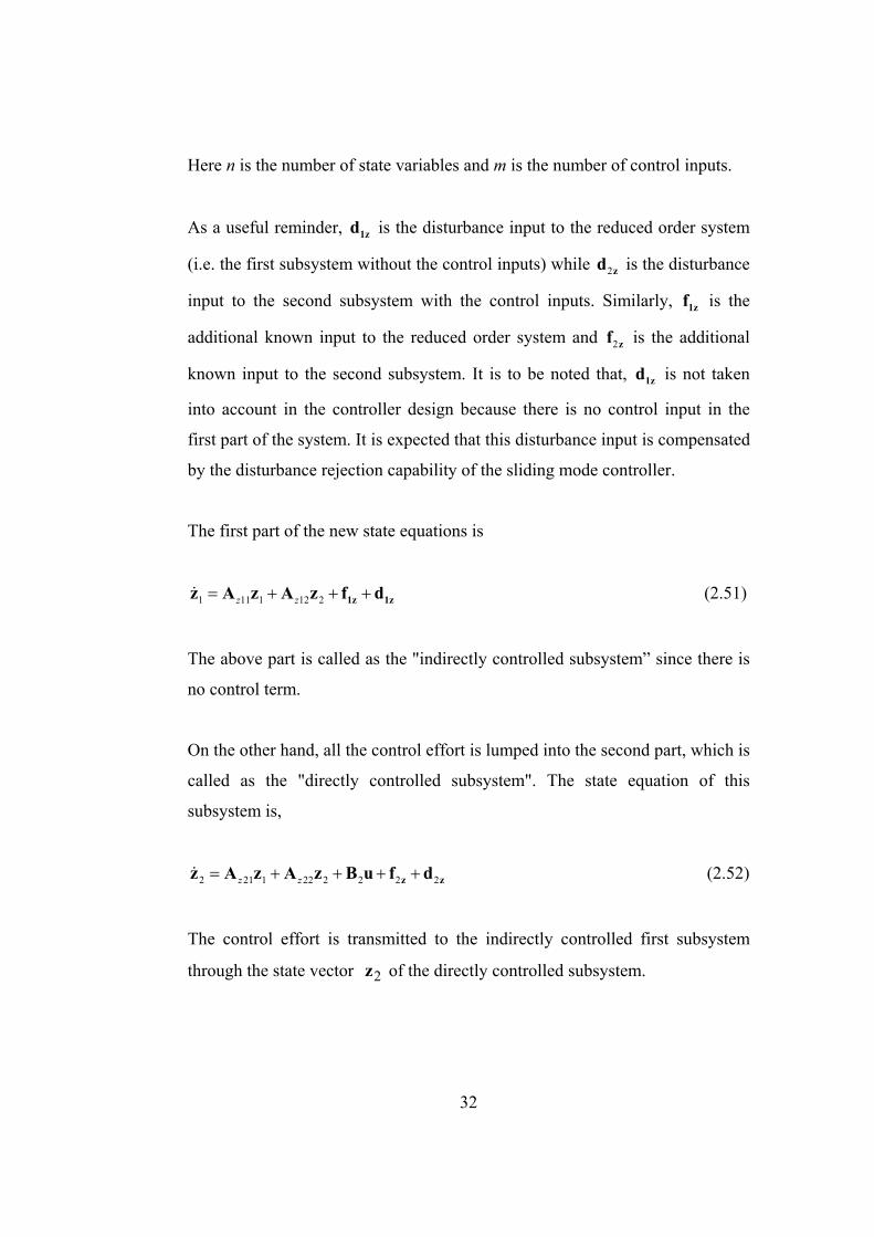
Here n is the number of state variables and m is the number of control inputs.
As a useful reminder, is the disturbance input to the reduced order system
(i.e. the first subsystem without the control inputs) while is the disturbance
input to the second subsystem with the control inputs. Similarly, is the
additional known input to the reduced order system and is the additional
known input to the second subsystem. It is to be noted that, is not taken
into account in the controller design because there is no control input in the
first part of the system. It is expected that this disturbance input is compensated
by the disturbance rejection capability of the sliding mode controller.
1zd
2zd
2zf
1zf
1zd
The first part of the new state equations is
1 11 1 12 2z z= + + +1z 1zz A z A z f d& (2.51)
The above part is called as the "indirectly controlled subsystem” since there is
no control term.
On the other hand, all the control effort is lumped into the second part, which is
called as the "directly controlled subsystem". The state equation of this
subsystem is,
32
22 21 1 22 2 2 2z z= + + + +z zz A z A z B u f d& (2.52)
The control effort is transmitted to the indirectly controlled first subsystem
through the state vector of the directly controlled subsystem. 2z

This transmission is realised by treating as if it is the control input to the
first subsystem. As such, it is formulated most typically according to the state
variable feedback control law so that
2z
33
1
m
in
)
2 2= −z h Cz (2.53)
Here, is the bias term added for the purpose of disturbance rejection and C
is the feedback gain matrix. Note that Eq. (2.53) defines a surface Ω (i.e. a
dimensional manifold) in the n dimensional state space of the whole
system. This surface is called the sliding surface. The deviation σ of the state
vector from the sliding surface is expressed as,
2h
mn −
2 1( ) = + − 2σ z z Cz h (2.54)
Using the surface-related terminology, is considered as the slope of the
sliding surface and h is considered as the offset of the sliding surface from the
origin of the state space. 2h ter is deliberately added to the classical sliding
surface equation in order to suppress the effects of 1zf and 1zd (2.51) as
much as possible.
C
2
When the system state is on the sliding surface, i.e. when
, Eq. (2.51) becomes; 2 1( ) 0= + − =2σ z z Cz h
1 11 12 1 12 2( ) (z z z= − + + +1z 1zz A A C z A h f d& (2.55)

Here, and must be determined in such a way that the closed-loop system
represented by Eq. (2.55) is asymptotically stable with a sufficiently fast
convergence and approaches the desired vector with a tolerable error.
C 2h
1z 1dz
After the sliding surface is determined as described above, the next stage of
controller design is to determine the actual control vector u so that the state of
the system is forced toward the sliding surface. In other words, u must be
determined so that σ is driven to zero and kept so despite the disturbances. This
purpose can be achieved by using the second stability theorem of Lyapunov as
described below.
Let T12
=V σ σ be defined as the Lyapunov function. Then, the following
condition must be satisfied to force to be zero. σ
T 0= <V σ σ& & (2.56)
This condition leads to the sliding mode controller (SMC) through the
following stages.
Recalling from equation (2.54), its derivative is written as ( )σ z
2 1 1( ) = + + − 2σ z z Cz Cz h& && & & (2.57)
21 1 22 2 2 2 2 11 1 12 2 1 1( ) ( )z z z z= + + + + + + + + + −z z 1z zσ z A z A z B u f d C A z A z f d Cz h& && 2
(2.58)
34

By using the condition that T 0<σ σ& ; SMC can be obtained as follows being
composed of two different controllers, i.e. as nom sw= +u u u .
(i) The nominal control:
1
nom 2 21 1 22 2 2 11 1 12 2 1( )z z z z− ⎡ ⎤= − + + + + + + −⎣ ⎦z 1zu B A z A z f C A z A z f Cz h& &
2 (2.59)
As noticed, the disturbances and are assumed to be zero in obtaining
the nominal control.
1zd 2zd
(ii) The switching control:
11sw 2
2
sgn( )sgn( )
σσ
− ⎡ ⎤= − ⎢ ⎥
⎣ ⎦u B K (2.60)
This control constituent is added in order to deal with the disturbances and
. Its derivation is explained below.
1zd
2zd
When equation (2.59) is substituted, Inequality (2.56) becomes,
[ ]T T2 sw 2 1 0= + +z zσ σ σ B u d Cd& < (2.61)
or,
[ ]T T2 sw 2 1 0+ +z zσ B u σ d Cd < (2.62)
Let,
35

eq 2 1 sw 2 sw and ′= + =z zd d Cd u B u (2.63)
Then,
T Tsw eq 0′ + <σ u σ d (2.64)
or,
36
<1 sw1 2 sw2 1 eq1 2 eq2 0u u d dσ σ σ σ′ ′+ + + (2.65)
Assume that,
eq1 1 eq2 2 and d D d< D< (2.66)
In the worst case,
eq1 1 1 eq2 2 2sgn( ) and sgn( )d D d Dσ σ= = (2.67)
Then,
1 sw1 2 sw2 1 1 2 2 0u u D Dσ σ σ σ′ ′+ + + < (2.68)
This condition can be satisfied by letting,
sw1 1 1 1sgn( )u k D σ′ = − (2.69)

and
sw2 2 2 2sgn( )u k D σ′ = − (2.70)
Such that,
1 21 and 1k k> > (2.71)
Hence, can be obtained as, swu
11 1sw 2 sw 2
2
sgn( )sgn( )
σσ
− − ⎡ ⎤′= = − ⎢⎣ ⎦
u B u B K ⎥
⎥
2
⎥
(2.72)
where,
1 1
2 2
00
k Dk D
⎡ ⎤= ⎢⎣ ⎦
K (2.73)
As a summary, SMC can be obtained as the sum of the following two control
constituents.
1
nom 2 21 1 22 2 2 11 1 12 2 1( )z z z z− ⎡ ⎤= − + + + + + + −⎣ ⎦z 1zu B A z A z f C A z A z f Cz h& & (2.74)
11sw 2
2
sgn( )sgn( )
σσ
− ⎡ ⎤= − ⎢
⎣ ⎦u B K (2.75)
37

In other words,
nom sw= +u u u (2.76)
Here is a matrix of tuning parameters for adjusting how fast the system
state will reach the sliding surface and how successfully the controller rejects
the disturbances. In other words, has two functions: disturbance rejection
function and forcing function on the state to drive it toward the sliding surface.
Its first function is explained above during the derivation. Its second function
can be explained as follows.
K
K
If K has small elements, reaching to the sliding surface is slow, but the
chattering amplitude and frequency are also small.
If K has large elements, reaching to the sliding surface is fast, but the
chattering amplitude and frequency are also large.
Here, chattering is defined as the in-and-out oscillation of the system state
about the sliding surface. This phenomenon arises due to the conflict between
the distracting effect of the disturbances and the restoring effect of the
switching parts of the control inputs.
As a summary, the larger the elements of K are, the more effective its two
functions become, but on the other hand, the more severely the chattering
phenomenon occurs. Figure 2.2 shows the effect of on the chattering
phenomenon. The “k” value in the figure is the amplitude of the chattering and
it is directly proportional to the elements of the selected K .
K
38

-k
k
unom
t
Figure 2.2 Effect of K on the Chattering Phenomenon
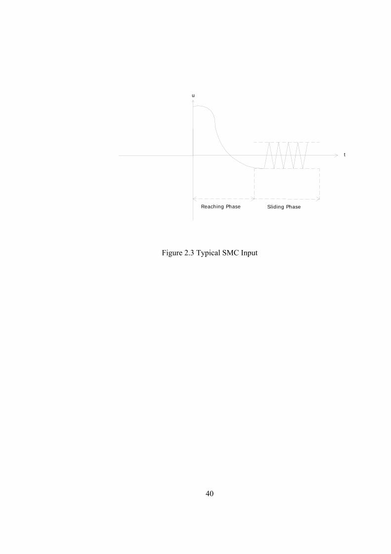
Figure 2.3 is given to explain the characteristic behaviour of the sliding mode
controller which is composed of two sub-controllers. The first part is defined as
the reaching phase and this is the part where the switching control is active and
forces the system states towards the sliding surface. The second part is defined
as the sliding phase and this is the part where the nominal control is active and
keeps the system states on the sliding surface.
39
u
Reaching Phase
t
Sliding Phase
Figure 2.3 Typical SMC Input
40

2.2.1.1 Determination of Sliding Surface Parameters
At first, sliding surface equation is defined, 2 1( ) = + − 2σ z z Cz h
2h
, and then the
sliding mode controller is designed based on this definition. But the parameters
of the sliding surface equation: sliding surface slope matrix, C and the offset
of sliding surface from the state space origin, are still not known.
There are different methods for determining the slope and the offset of the
sliding surface but in this study, they are determined by solving the State
Dependent Riccati Equations (SDRE) so that they become adaptive to the
nonlinearities of the system. By this methodology, the problem of sliding
surface determination is reduced to a Linear Quadratic Regulator (LQR)
problem including bias terms.
In other words, the slope (C) and the offset (h2) of the sliding surface are
determined so as to minimise the following cost functional.
( ) ( ) ( ) ( )( )T T1 1 11 1 1 2 2 22 2 2
1 dt2
st
J∞
= − − + − −∫ z r Q z r z r Q z r (2.77)
Here, represents the steady state values at the desired position for the
reduced order system while represents the steady state values at the desired
position for the second subsystem. and are properly specified
weighting matrices which may be functions of the state variables if desired.
The desired final values of the state variables are expressed in more detail as
follows.
1r
2r
11Q 22Q
41

42
⇒
1 11
2 121
3 132
4 21
5 22
d
d
d
d
d
x rx rx rx rx r
⎡ ⎤ ⎡ ⎤⎢ ⎥ ⎢ ⎥⎢ ⎥ ⎢ ⎥⎡ ⎤⎢ ⎥ ⎢ ⎥= = =⎢ ⎥⎢ ⎥ ⎢ ⎥⎣ ⎦⎢ ⎥ ⎢ ⎥⎢ ⎥ ⎢ ⎥⎣ ⎦⎣ ⎦
d
rTx T
r (2.78)
11
1 12
13
and, rrr
⎡ ⎤⎢ ⎥= ⎢ ⎥⎢ ⎥⎣ ⎦
r (2.79)
212
22
rr⎡ ⎤
= ⎢ ⎥⎣ ⎦
r (2.79)
where includes the steady state values for the system state variables. dx
In the general multivariable case, the SDRE nonlinear feedback solution and its
associated state and costate trajectories satisfy the first necessary condition for
optimality ( 2 0∂ ∂ =H z ) of the nonlinear optimal regulator problem (2.77).
Additionally, if , , and along with their gradients are
bounded in a neighborhood about the origin, under asymptotic stability, as the
state is driven to zero, the second ecessary condition for optimality
(
11zA 12zA 11Q 22Q
1z
1 = −∂ 1∂λ H z& ) asymptotically satisfied at a quadratic rate. [28]
where H represents the Hamiltonian function and defined by,
( ) ( ) ( ) ( )T T T1 1 11 1 1 2 2 22 2 2 1 1
1 1 ( )2 2
= − − + − − +H z r Q z r z r Q z r λ z& (2.81)
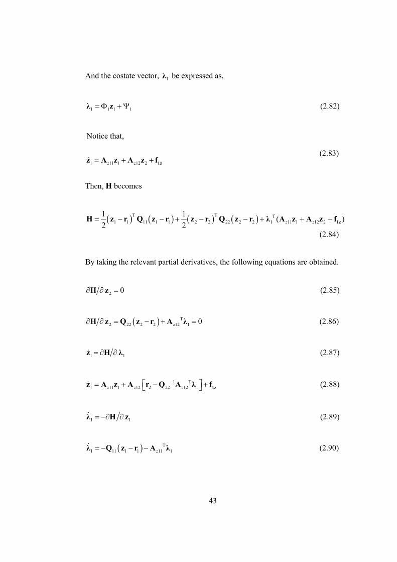
And the costate vector, be expressed as, 1λ
43
11 1 1= Φ +Ψλ z (2.82)
1 11 1 12 2
Notice that,
z z= + + 1zz A z A z f& (2.83)
Then, H becomes
( ) ( ) ( ) ( )T T T1 1 11 1 1 2 2 22 2 2 1 11 1 12 2
1 1 ( )2 2 z z= − − + − − + + + 1zH z r Q z r z r Q z r λ A z A z f
(2.84)
By taking the relevant partial derivatives, the following equations are obtained.
2 0∂ ∂ =H z (2.85)
( ) T2 22 2 2 12 1 0z∂ ∂ = − + =H z Q z r A λ (2.86)
1 = ∂ ∂z H λ& 1
⎤⎦
(2.87)
1 T
1 11 1 12 2 22 12 1z z z−⎡= + − +⎣ 1zz A z A r Q A λ f& (2.88)
1 = −∂ ∂λ H z&1 (2.89)
( ) T1 11 1 1 11z= − − −λ Q z r A λ&
1 (2.90)

By using the equation (2.86), the control structure can be expressed as follows,
1 T
2 2 22 12 1z−= −z r Q A λ (2.91)
Finally equation (2.53), equation (2.90) and equation (2.91) can be combined
as,
1 T 1 T
2 2 22 12 1 1 22 12 1 1z z− −= − Φ − Ψ = − + 2z r Q A z Q A Cz h (2.92)
Hence, the slope and offset of the sliding surface can be defined as
follows.
C 2h
1 T
22 12 1z−= ΦC Q A (2.93)
44
1
1
1 T2 22 12z
−= − Ψ2h r Q A (2.94)
Then,
1 1 1 1 1 1 1 1 1= Φ +Ψ ⇒ =Φ +Φ +Ψλ z λ z z& && & (2.95)
The final equation is derived by combining Equations (2.90) and (2.95). That
is,
( ) T1 11 1 1 11 1 1 1 1 1z= − − − = Φ +Φ +Ψλ Q z r A λ z z& && & 1 (2.96)
This equation implies that

( ) ( )[ ]( )
T11 1 1 11 1 1 1
1 T1 1 1 11 1 12 2 12 22 12 1 1 1 1
z
z z z z−
− − − Φ +Ψ
= Φ +Φ + − Φ +Ψ + +Ψ1z
Q z r A z
z A z A r A Q A z f && (2.97)
By equating the coefficients of , the following two equations can be
obtained;
1z
45
1 Tz
Ψ
T11 11 1 1 1 1 11 1 12 22 12 1z z z
−− − Φ = Φ +Φ −Φ ΦQ A z A A Q A& (2.98)
T 1 T
11 1 11 1 1 12 2 1 12 22 12 1 1 1 1z z z z−− Ψ = Φ −Φ Ψ +Φ +1zQ r A A r A Q A λ f & (2.99)
The above equations are solved for the steady state conditions by taking the
derivatives equal to zero.
The first equation leads simply to the following algebraic matrix Riccati
equation,
T 1 T
1 11 11 1 1 12 22 12 1 11 0z z z z−Φ + Φ −Φ Φ + =A A A Q A Q (2.100)
This equation is solved for 1Φ .
The steady state form of the second equation is
T 1
11 1 11 1 1 12 2 1 12 22 12 1 1z z z z−− Ψ = Φ −Φ Ψ +Φ 1zQ r A A r A Q A fT (2.101)
This equation can be rearranged as

( ) ( )T 1 T11 1 12 22 12 1 11 1 1 12 2z z z z
−− + Φ Ψ = − + Φ + 1zA A Q A Q r A r f
]
(2.102)
1Hence, is found as follows.Ψ
( ) [( )1T 1 T1 11 1 12 22 12 11 1 1 12 2z z z z
−−Ψ = − +Φ − +Φ + 1zA A Q A Q r A r f (2.103)
Since and are known, the slope and the offset of the sliding surface can
be determined as shown below.
1Φ 1Ψ
1 T
22 12 1z−= ΦC Q A (2.104)
1 T
2 22 12z−= − Ψ2h r Q A 1 (2.105)
The sliding mode controller is designed with a moving sliding surface such that
its parameters, sliding surface slope and the offset of sliding surface, are
determined in an adaptive manner and optimally selected for the given
weighting matrix, . In other words, sliding surface slope and the offset of
sliding surface are determined and sliding mode controller can be derived
using the equations (2.74), (2.75) and (2.76).
Q C
2h
The use of “sign” function may yields numerical errors as a result of the
insufficient integration time step selection during numerical calculations.
Furthermore, because of the discontinuity across the sliding surfaces, the
preceding control law may result in control chattering. As a practical matter,
chattering is undesirable because it involves high frequency switched control
action and may excite high frequency dynamics neglected in the modelling.
46

Therefore, to minimise these drawbacks, tangent hyperbolic function is used
instead of sign function in the case study simulations. Thus, the following form
is used in the case study simulations.
47
⎥1 11
sw 22 2
tanh( )tanh( )
cc
σσ
− ⎡ ⎤= − ⎢
⎣ ⎦u B K (2.106)
where c1 and c2 are the parameters used to adjust the slope of the tangent
hyperbolic function.

2.2.2 Pure SDRE Method
After the system dynamics is expressed in the form given by Equation (2.29),
instead of designing a sliding mode controller, an ordinary feedback controller
may also be designed. This controller is considered here for the sake of
comparison with the SDRE-based SMC. Proposed SDRE-based SMC can also
be compared different cases such as the SMC designed for the model linearised
about the initial and/or final conditions or the SMC designed with constant
sliding surface parameters i.e., the sliding surface slope and the offset of
sliding surface. The reason why pure SDRE method, which the derivation is
explained below, is selected as a comparision criteria for the proposed SDRE-
based SMC is that; it is obvious that proposed SDRE-based SMC have much
more better performances compared with the above two cases. But it is not as
easy to say the same for the pure SDRE method without doing a case study.
The gain and the bias term of this feedback controller can again be determined
by means of solving the State Dependent Riccati Equations. This means that
the parameters of the ordinary feedback controller are also adapted in the same
manner with those of the sliding mode controller.
In order to design this controller, the cost functional is taken as
( ) ( )T Td d
0
1 dt2
J∞
⎡= − − +⎣∫ x x Q x x u Ru% % % % ⎤⎦
b
(2.107)
The control input can be expressed as
= − +u Gx% (2.108)
48

Here, represents the gain of the feedback controller while b represents the
bias term.
G
Hamiltonian is defined as
( ) ( )T T Td d 1
1 1 ( )2 2
= − − + +H x x Q x x u Ru λ x&% % % % % (2.109)
Note that,
( ) ( ) ( ) ( )= + + +x A x x B x u f x d x&% % % % % % (2.110)
The unknown disturbance term is not taken into account in the design of
this controller. So,
( )d x%
( ) ( ) [ ]T T Td d 1
1 1 ( ) ( ) ( )2 2
= − − + + + +H x x Q x x u Ru λ A x x B x u f x% % % % % % % % (2.111)
However, as may be recalled, was taken into account with the estimated
upper bounds of its components in designing the switching control of SMC.
( )d x%
By taking the relevant partial derivatives, the following equations are obtained.
0∂ ∂ =H u (2.112)
T
1 0∂ ∂ = + =H u Ru B λ (2.113)
1 T
1−= −u R B λ (2.114)
49

1= ∂ ∂x H λ&% (2.115)
1 T
1 ( )−⎡ ⎤= + − +⎣ ⎦x Ax B R B λ f x&% % % (2.116)
1 = −∂ ∂λ H x& %&
1
1
1
(2.117)
( ) T1 d= − − −λ Q x x A λ& % % (2.118)
Let costate vector be expressed as in (2.82),
1 1= Φ +Ψλ x%
The derivative of the costate vector is as follows,
1 1 1= Φ +Φ +Ψλ x x& & && % % (2.119)
Then the equations (2.117) and (2.119) are combined as
( ) ( ) ( )T 11 d 1 1 1 1 1 ( )−⎡ ⎤= − − − Φ +Ψ = Φ +Φ + − + +Ψ⎣ ⎦λ Q x x A x x Ax B R B λ f x& &&% % % % % %T
1
1 T1
(2.120)
By equating the coefficients of the , the following two equations are
obtained.
x%
T
1 1 1 1−− − Φ = Φ +Φ −Φ ΦQ A A BR B& (2.121)
50

( )T 1 Td 1 1 1 1
−− Ψ = −Φ Ψ +Φ +ΨQx A BR B f x &% 1% (2.122)
The above equations are solved for the steady state conditions by taking the
derivatives equal to zero. The first equation leads simply to the following
algebraic matrix Riccati equation,
T 1 T
1 1 1 1 0−Φ + Φ −Φ Φ + =A A BR B Q (2.123)
This equation is solved for 1Φ .
The steady state form of the second equation is
( )T 1 Td 1 1 1 1
−− Ψ = −Φ Ψ +ΦQx A BR B f x% % (2.124)
This equation can be solved for Ψ1 as
( ) ( )( )1T 1 T1 1 d 1
−−Ψ = − +Φ − +ΦA BR B Qx f x% % (2.125)
Since and are known, the gain of the feedback controller and the bias
term can be determined by combining the equations (2.108) and (2.114) so
that,
1Φ 1Ψ
1 T
1−= ΦG R B (2.126)
1 T
1−= − Ψb R B (2.127)
51

52
CHAPTER 3
APPLICATION OF THE DESIGNED CONTROLLER
TO A HYPERSONIC AIR VEHICLE MODEL This section includes the application of the proposed adaptive SMC to the
generic hypersonic vehicle model which was also studied in the main reference
article [10] and the result of the case study simulations. This case study
example is used mainly for comparison purposes with an alternative adaptive
SMC applied to the same vehicle in [10]. The units used in the case study
simulations are kept same with the ones in [10] during plotting phase to allow
us to compare the results.

3.1 Mathematical Model of the Hypersonic Air Vehicle The model which was also studied in the main reference article [10] is used in
this thesis study.
3.1.1 Nomenclature
A
Speed of Sound, m/s (ft/s)
DC
Drag Coefficient
LC
Lift Coefficient
( )MC q
Moment Coefficient due to Pitch Rate
( )MC α
Moment Coefficient due to Angle of Attack
( )M eC δ
Moment Coefficient due to Elevator Deflection
TC
Thrust Coefficient
C
Reference Length, 24.4 m (80 ft)
D
Drag, N (lbf)
h
Altitude, m (ft)
yyI
Moment of Inertia, 9.5 x10⁶ kg-m
2 (7x10
6 slug-ft
2)
53

L
Lift, N (lbf)
M
Mach Number
yyM
Pitching Moment, N.m (lbf-ft)
m
Mass, 136818 kg (9375 slugs)
q
Pitch Rate, rad/s
ER
Radius of the Earth, 6371400 m (20903500 ft)
r
Radial Distance from Earth’s center, m (ft)
S
Reference Area, 335 m2 (3603 ft
2)
T
Thrust, N (lbf)
V
Velocity, m/s (ft/s)
α
Angle of Attack, rad
β
Throttle Setting
γ
Flight-Path Angle, rad
eδ
Elevator Deflection, rad
μ
Gravitational Constant , 3.94 x10¹⁴
m3 /s
2 (1.39x10
16 ft
3 /s
2)
ρ
Density of Air, 0.013 kg/m3 (
0.24325x10
-4 slugs/ft
3 )
54

3.1.2 Differential Equations of the System
A simplified version of the model used in [12] and [15] has been presented in
[10]. The model describing the longitudinal dynamics of a generic hypersonic
air vehicle has been simplified by making appropriate modifications for the
trimmed cruise condition (M=15, V=4,590 m/s (15,060 ft/s), h=33,528 m
(110,000 ft), γ=0 deg, and q=0 deg/s). The equations of motions derived for
this vehicle include an inverse-square-law gravitational model, and the
centripetal acceleration for the nonrotating Earth.
Figure 3.1 Free Body Diagram of a Simplified Hypersonic Air Vehicle
(Resource: Adaptive Predictive Expert Control, [14])
55
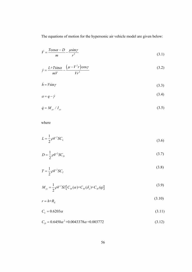
The equations of motion for the hypersonic air vehicle model are given below:
(3.1) (3.2)
56
(3.3) (3.4)
(3.5)
( )
2
2
cos sin
cos+ sin
sin
2
yy yy
T DVm r
V rL TmV Vr
h V
a q
q M / I
α μ γ
μ γαγ
γ
γ
−= −
−= −
=
= −
=
&
&
&
&
&
where
(3.6) (3.7)
(3.8)
(3.9)
(3.10)
[
2
e
12
12
12
1 ( )+ ( )+2
+
2L
D
2T
2yy M M M
E
L V SC
D V SC
T V SC
]M V Sc C C C (q)
r h R
ρ
ρ
ρ
ρ α δ
=
=
=
=
=
0.6203LC α= (3.11)
20.6450 +0.0043378 +0.003772DC α α= (3.12)

0.02576 , ( <1)0.02240 0.00336 , ( >1)TC
β ββ β
⎧= ⎨ +⎩
(3.13)
57
-6
2( ) 0.035 +0.036617 +5.3261×10MC α α α= − (3.14)
( ) 2( ) ( 6.796 +0.3015 0.2289)MC q c 2V q α α= − − (3.15)
(e e( )M eC c )δ δ α= − (3.16) where it is assumed that ce remains constant as 0.0292ec = .

3.2 Sliding Mode Control Design for the Hypersonic Air Vehicle Model
The hypersonic air vehicle can be modelled as follows.
=x a(x) + B(x)u& (3.17)
where
1
2
3
4
5
x Vxx hxx q
γ
α
⎡ ⎤⎡ ⎤⎢ ⎥⎢ ⎥⎢ ⎥⎢ ⎥⎢ ⎥⎢ ⎥= =⎢ ⎥⎢ ⎥⎢ ⎥⎢ ⎥⎢ ⎥⎢ ⎥⎣ ⎦ ⎣ ⎦
x
&&
& &
&& &
& &
& &
and, (3.18)
1 e
2
uu
δβ
⎡ ⎤ ⎡ ⎤= =⎢ ⎥ ⎢ ⎥
⎣ ⎦⎣ ⎦u (3.19)
By rearranging the differential equations of the system, it is seen that
{ }( )
( )
22
2
2
2
2
2
2
sin(0.6450 +0.0043378 +0.003772)
2 ( )
cos0.6203
2 ( + )
sin
( + )cos0.6203
2 ( + )
( 0.2
( )
+
1 24 4
3
214
1 3 e
1 2
1 3 e 214
1 3 e
1
e
1 3 e
5
yy
Sx xx x
m x + R
xSxx
m x x R
x x
x x R xSxx x
m x x R
SxI
c
x x R
ρ μ
ρ
μρ
ρ
μ
−−
−
−− −
−
=
⎧ ⎫⎨ ⎬⎩ ⎭
⎧ ⎫−⎪ ⎪⎨ ⎬⎪ ⎪⎩ ⎭
⎧ ⎫⎛ ⎞⎪ ⎪⎜ ⎟⎨ ⎬⎜ ⎟⎪ ⎪⎝ ⎠⎩ ⎭
xa
( )2 -6 2035 + +5.3261e )+ ( 6.796 +0.300. 15 0.2289)0366174 4 4 41
e 5x x x xc x2xc
− −−⎧
⎡ ⎤⎢ ⎥⎢ ⎥⎢ ⎥⎢ ⎥⎢ ⎥⎢ ⎥⎢ ⎥⎢ ⎥⎢ ⎥⎢ ⎥⎢ ⎥⎢ ⎫
⎨ ⎬⎥
⎢ ⎥⎢ ⎦⎩ ⎭⎥⎣
(3.20)
58

( )
( )
( )
2
2
2
0.02576cos2
0.02576s
0
0
0 0
0
in2
0.02576cos
20
2
14
14
14
1
y
e
y
Sx xmSx xm
Sx xm
Sx ccI
ρ
ρ
ρ
ρ
=
⎡ ⎤⎢ ⎥⎢ ⎥⎢ ⎥⎢ ⎥⎢⎢⎢ ⎥⎢ ⎥⎢ ⎥⎢ ⎥⎢ ⎥⎢ ⎥⎣ ⎦
−B(x)
⎥⎥
%
(3.21)
However, the state equation of the system that is going to be controlled with
this methodology should be in the following form:
( ) ( ) ( )= + +x A x x B x u d x& (3.22)
In this study, the required form is obtained as follows for the hypersonic air
vehicle.
( ) ( ) ( ) ( )= + + +x A x x B x u f x d x&% % % % % (3.23)
where
1
2
3
4
5
Vxxx hxx q
γ
α
⎡ ⎤⎡ ⎤⎢ ⎥⎢ ⎥⎢ ⎥⎢ ⎥⎢ ⎥⎢ ⎥= =⎢ ⎥⎢ ⎥⎢ ⎥⎢ ⎥⎢ ⎥⎢ ⎥⎣ ⎦ ⎣ ⎦
x
%%
%% % and, 1
2
euu
δβ
⎡ ⎤ ⎡ ⎤= =⎢ ⎥ ⎢ ⎥
⎣ ⎦⎣ ⎦u (3.24)
By rearranging the differential equations of the system, the following set of
equations can be obtained,
59
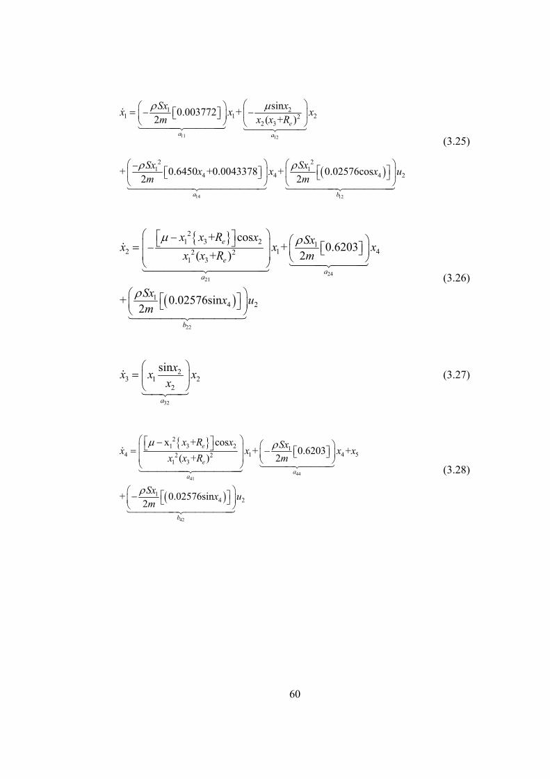
( )
11 12
14 12
1 21 1 22
2 3
2 21 1
4 4
sin0.003772 +2 ( + )
+ 0.6450 +0.0043378 + 0.02576cos2 2
ea a
a b
Sx xx x xm x x R
Sx Sx4 2x x x
m m
ρ μ
ρ ρ
⎛ ⎞− −⎡ ⎤ ⎜ ⎟⎣ ⎦
⎝ ⎠
⎛ ⎞ ⎛− ⎡ ⎤⎡ ⎤⎜ ⎟ ⎜⎣ ⎦
⎛ ⎞⎜ ⎟⎝
⎣ ⎦⎝ ⎠ ⎝
⎠=14444244443 1442443
144444424444443 1444442444443
&
u⎞⎟⎠
(3.25)
{ }
( )
2421
22
21 3 2 1
2 12 21 3
14 2
+ cos+ 0.6203
( + ) 2
+ 0.02576sin2
e
ea
a
b
x x R x Sx4x x x
x x R m
Sx x um
μ ρ
ρ
⎛ ⎞⎜ ⎟⎜ ⎟⎝ ⎠
⎡ ⎤− ⎛ ⎞⎣ ⎦− ⎡ ⎤⎜ ⎣ ⎦ ⎟⎝ ⎠
⎛ ⎞⎡ ⎤⎜ ⎟⎣ ⎦⎝ ⎠
=1444244431444442444443
14444244443
&
(3.26)
32
23 1
2
sin
a
x2x x x
x⎛ ⎞⎜ ⎟⎝ ⎠
=14243
& (3.27)
{ }
( )
4441
42
21 3 2 1
54 12 21 3
14 2
x + cos+ 0.6203 +
( + ) 2
+ 0.02576sin2
e
ea
a
b
x R x Sx4x x x
x x R m
Sx x um
μ ρ
ρ
⎡ ⎤ ⎛ ⎞⎣ ⎦ ⎡⎛ ⎞⎜ ⎟⎜ ⎟
⎤⎜ ⎣ ⎦ ⎟⎝ ⎠
⎛ ⎞⎡ ⎤⎜ ⎟⎦ ⎠
⎠
⎣⎝
⎝
−−
−
=1444244431444442444443
1444442444443
& x
(3.28)
60

51
54
-615 1
51 14 4
1
5.3261e2
+ 0.035 + + 6.796 +0.30152 4
0.03661
+ 0.2284
7
yy
a
2 2
yy yy
a
2
y
e
y
c
c c
Sxx xI
Sx Sx x4x x x
I Ic
cSxI
ρ
ρ ρ
ρ
⎡ ⎤⎣ ⎦
⎛ ⎞⎧ ⎫ ⎧⎪ ⎪ ⎪⎜
⎛ ⎞⎜ ⎟⎜
⎟⎡ ⎤ ⎡⎨ ⎬ ⎨⎣ ⎦ ⎣⎜ ⎟
⎟⎝ ⎠
⎪ ⎪ ⎪⎩ ⎭ ⎩⎝ ⎠−
=
− −
−
14444244443
144444444444444424444444444444443
&
⎫⎪⎤⎬⎦⎪⎭
55 51
15 2
a
9 +2
2
yye
b
cSxx uI
cρ⎛ ⎞⎜ ⎟⎜
⎛ ⎞⎡ ⎤ ⎜ ⎡ ⎤ ⎟⎣ ⎦ ⎣ ⎦⎜ ⎟
⎝⎟
⎝ ⎠⎠14444244443 1442443
(3.29)
The arrangements made above in order to obtain the state dependent
coefficients are of course not unique. Here, the arrangement is preferred to be
such that the system state variables which are physically changing in a
relatively fast manner such as the angle of attack, the flight path angle and the
pitch rate are factored out as linear multipliers of the state dependent
coefficients (i, j = 1 to 5). ija
One of the factors that the performance of the controller over the domain of
interest is state dependent coefficient (SDC) matrix . In the multivariable
case, the SDC parameterisation is not unique and there is no systematic way to
express as . By definition, the pair
( )A x
( )a x ( )A x x { }( ), (A x B )x is a controllable
(stabilisable) parameterisation of the nonlinear system in a region if Ω
{ }( ),A x
∈Ωx
( )B x is pointwise controllable (stabilisable) in the linear sense for all
. This definition is used to guarantee that the SDRE nonlinear regulator
produces a closed-loop solution which is locally asymptotically stable [15].
61
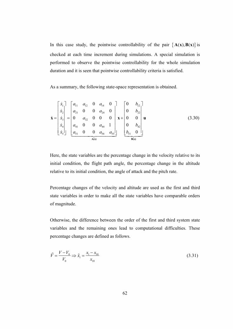
In this case study, the pointwise controllability of the pair { }( ), ( )A x B x is
checked at each time increment during simulations. A special simulation is
performed to observe the pointwise controllability for the whole simulation
duration and it is seen that pointwise controllability criteria is satisfied.
As a summary, the following state-space representation is obtained.
1 11 12 14 12
2 21 24 22
3 32
4 41 44 42
5 51 54 55 51
0 0 00 0 0 0
0 0 0 0 0 00 0 1 00 0 0
x a a a bx a a bx ax a a bx a a a b
⎡ ⎤ ⎡ ⎤ ⎡ ⎤⎢ ⎥ ⎢ ⎥ ⎢ ⎥⎢ ⎥ ⎢ ⎥ ⎢ ⎥⎢ ⎥ ⎢ ⎥ ⎢ ⎥= = +⎢ ⎥ ⎢ ⎥ ⎢ ⎥⎢ ⎥ ⎢ ⎥ ⎢ ⎥⎢ ⎥ ⎢ ⎥ ⎢ ⎥⎣ ⎦ ⎣ ⎦ ⎣ ⎦
A(x) B(x)
x
&
&
& &
&
&
x u
14444244443 14243
(3.30)
Here, the state variables are the percentage change in the velocity relative to its
initial condition, the flight path angle, the percentage change in the altitude
relative to its initial condition, the angle of attack and the pitch rate.
Percentage changes of the velocity and altitude are used as the first and third
state variables in order to make all the state variables have comparable orders
of magnitude.
Otherwise, the difference between the order of the first and third system state
variables and the remaining ones lead to computational difficulties. These
percentage changes are defined as follows.
0 11
0 1
V V x xV xV x− −
= ⇒ =% % 10
0
(3.31)
62

therefore,
63
) (1 10 11x x x= + % (3.32)
and,
1 1 10x x x= && % (3.33)
0 33
0 3
x h - h x - xhh x
= ⇒ =% % 30
0
(3.34)
therefore,
( )3 30 31 x x x= + % (3.35)
and,
3 3 30x x x= && % (3.36)
As the next step, the change in first and third system state variables in terms of
percentage change relative to their initial conditions are reflected to the above
state space representation in Eqn. (3.30). The following equations are obtained,
1 11 1 12 2 14 4 12 21
10 10
; x a x +a x +a x +b uxx x
= =&&% (3.37)
(1 10 11 ) x x x= + % (3.38)

64
) (3 30 31x x x= + % (3.39)
( )11 10 1 12 2 14 4 12 211
10 10
1a x + x +a x +a x +b uxxx x
⎡ ⎤⎣ ⎦= =%&&% (3.40)
12 14 121 11 11 1 2 4
10 10 10
a a b2x a a x x x u
x x x= + + + +&% % (3.41)
2 21 1 24 4 22 2; x a x a x b u= + +& (3.42)
(1 10 11 ) x x x= + % (3.43)
( )3 30 31 x x x= + % (3.44)
( )2 21 10 1 24 4 221 2x a x x a x b u= + + +⎡ ⎤⎣ ⎦& % (3.45)
( )2 21 10 21 10 1 24 4 22 2x a x a x x a x b u= + + +& % (3.46)
3 3 32 2 323
30 30 30 30
x x a x a2x x
x x x x= = = =& &&% (3.47)
4 41 1 44 4 5 42 2; x a x a x x b u= + + +& (3.48)

( )1 10 11 x x x= + % (3.49)
( )3 30 31 x x x= + % (3.50)
( )4 41 10 1 44 4 5 42 21x a x x a x x b u= + + + +⎡ ⎤⎣ ⎦& % (3.51)
( )4 41 10 41 10 1 24 4 5 42 2x a x a x x a x x b u= + + + +& % (3.52)
(3.53)
5 51 1 54 4 55 5 51 1; x a x a x a x b u= + + +&
( )1 10 11 x x x= + % (3.54)
( )3 30 31 x x x= + % (3.55)
( )5 51 10 1 54 4 55 5 51 11x a x x a x a x b u= + + + +⎡ ⎤⎣ ⎦& % (3.56)
( )5 51 10 51 10 1 54 4 55 5 51 1x a x a x x a x a x b u= + + + +& % (3.57)
ere, the state dependent coefficients i, j = 1 to 5) are also re-calculated H ija (
with the change of ( ) ( )1 and 1 1 10 1 30 33x x x x x x= + = +% % but the same notation is
used to prevent amb
iguity. As an example,
111 0.003772
2Sxm
ρa = − ⎡ ⎤⎣ ⎦ (3.58)
65

66
nd, a
( )1 10 11 x x x= + % (3.59)
o the new coefficient is determined as follows, S 11a
( ){ }10 111
1 0.003772
2x x
aS
mρ
− ⎦+
= ⎡ ⎤⎣%
(3.60)
he updated state space representation is as follows, T
11 12 10 14 10 12 10 111
21 10 24 22 212
32 303
41 10 44 424
51 10 54 55 515
0 0 00 0 0 0
= 0 0 0 0 + 0 0 +0 0 1 00 0 0
a a x a x b x axa x a b a xx
a xxa x a bxa x a a bx
⎡ ⎤ ⎡ ⎤ ⎡⎢ ⎥ ⎢ ⎥ ⎢⎢ ⎥ ⎢ ⎥ ⎢⎢ ⎥ ⎢ ⎥ ⎢=⎢ ⎥ ⎢ ⎥ ⎢⎢ ⎥ ⎢ ⎥ ⎢⎢ ⎥ ⎢ ⎥ ⎢⎣ ⎦ ⎣⎣ ⎦
A(x) B(x)
x x
% %
&%
&& &% %%
&
&144444424444443 1442443
10
41 10
51 10
0a xa x
⎡ ⎤⎢ ⎥⎢ ⎥⎢ ⎥⎢ ⎥⎢ ⎥⎢ ⎥⎣ ⎦
f(x)%14243
⎤⎥⎥⎥⎥⎥⎥⎦
u
(3.61)
should be noted that the term , appears in the updated system state
ew d
astly, the state dependent disturbance is added to the system. Disturbance is
It ( )f x%
representation as a result of this n efinition of the first and third system
state variables.
L
assumed as the wind effect which affects the related aerodynamic coefficients
by changing the angle of attack of the aircraft relative to the wind. It is
assumed that the disturbance effect is additive and affects only the angle of
attack dependent aerodynamic coefficients: LC , DC and MC (a) .

67
he additional disturbance terms are given below, T
C w0.6203ΔLw α= (3.62)
(3.63)
6 (3.64)
here,
2w w0.6450Δ +0.0043378Δ +0.003772D w α α=C
2 -w w(α) 0.035Δ +0.036617Δ +5.3261×10
wM α α= − C
w
Δ wα is the additional angle of attack and equal to the difference between the
aircraft angle of attack α and the angle of attack relative to the wind wα . wα
is the result of the comb ation of the aircraft speed and wind speed whin ile α is
the aircraft angle of attack measured when there is no wind.
Additional angle of attack term is defined as a fluctuating signal around its
non-zero mean value. The expression is as following,
( ) ( )( )w
w1w2
ΔΔ
Δ 0.25°+0.025° sin +sin 3 +sin 5t t tα
α
α ⎡ ⎤ ⎡ ⎤= − ⎣ ⎦ ⎣ ⎦12314444444244444443
(3.65)
Δ w1 0.25°α = − (3.66)
( ) ( )( )w2Δ = 0.025° sin +sin 3 +sin 5t t tα ⎡ ⎤ ⎡ ⎤⎣ ⎦ ⎣ ⎦ (3.67)

68
he expression in (3.65) is carefully selected to guarantee that harmonics and
ift and Drag forces and pitching moment are affected by the addition of these
T
repeated terms are avoided. In other words, by injecting the irrational numbers
into the sine functions, a mimicking random signal is generated for the
computer simulations.
L
coefficients. Since,
12
2w LwSCρ= (3.68)
L V
12
2w DD wV SCρ= (3.69)
1 ( )2w w
2yy MM V Sc Cρ α⎡ ⎤= ⎣ ⎦ (3.70)
he constant parts of the additional disturbance terms occurred as a result of
T
the new lift and drag forces and pitching moment are embedded inside the
system matrix ( )A x% and ( )f x% to guarantee that they can be compensated by
the sliding mode control The fluctuating parts on the other hand are
represented by the addition ( )d x% matrix to the state space representations.
( )d x% is given below,
ler.
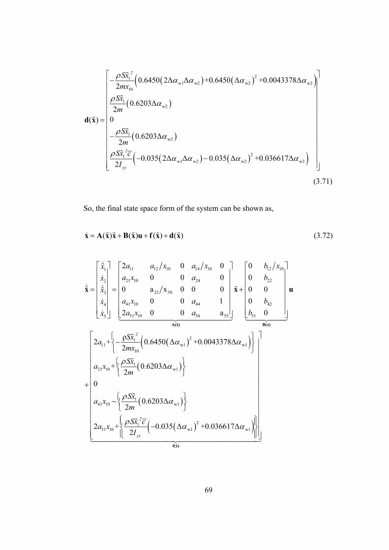
( ) ( )( )( )
( )
( ) ( )( )
w1 w2 w2 w210
w2
w2
w1 w2 w
21
1
1
22 w
1
0.6450 2Δ Δ +0.6450 Δ +0.0043378Δ
0.6203Δ
0( )
0.6203Δ
0.035 2Δ Δ 0.035 Δ +0.036
2
Δ
2
617
2
2
2
2
yy
Sxm
Sxm
Sxm
SxI
x
c
α α α α
α
α
α α α α
ρ
ρ
ρ
ρ
⎡ ⎤⎢ ⎥⎢ ⎥⎢ ⎥⎢ ⎥⎢ ⎥
= ⎢ ⎥⎢ ⎥⎢ ⎥⎢ ⎥⎢ ⎥⎢ ⎥⎢
−
−
⎥⎣ ⎦− −
d x%
%
%
%
%
2
(3.71)
o, the final state space form of the system can be shown as,
% (3.72)
S
( ) ( ) ( ) ( )= + + +x x B x u f x d x& % % % % x A
11 12 10 14 10 12 101
21 10 24 222
32 303
41 10 44 424
51 10 54 55 515
11
2 0 0 00 0 0 0
0 a x 0 0 0 0 00 0 1 0
2 0 0 a 0
2 +
a a x a x b xxa x a bx
xa x a bx
a x a bx
a
⎡ ⎤ ⎡ ⎤ ⎡ ⎤⎢ ⎥ ⎢ ⎥ ⎢ ⎥⎢ ⎥ ⎢ ⎥ ⎢ ⎥⎢ ⎥ ⎢ ⎥ ⎢ ⎥= = +⎢ ⎥ ⎢ ⎥ ⎢ ⎥⎢ ⎥ ⎢ ⎥ ⎢ ⎥⎢ ⎥ ⎢ ⎥ ⎢ ⎥⎣ ⎦
−
⎦⎣ ⎦
+
A(x) B(x)
x x
%
&%
&& &% %%
&
& ⎣
u
144444424444443 1442443
( )( )
( )
( )
( )( )
2w1 w1
10
21 10 w1
41 10 w1
51 10 w1 w1
1
1
1
21
0.6450 Δ +0.0043378Δ
+ 0.6203Δ
0
0.6203Δ
2 + 0.035 Δ +0
ρ2
.036
2
2
2617Δ
2
2
yy
x
a x
a x
c
Sxm
Sxm
Sxm
Sxa xI
α α
α
α
α α
ρ
ρ
ρ
⎡ ⎤⎧ ⎫⎨ ⎬⎢ ⎥⎩ ⎭⎢ ⎥
⎢ ⎥⎧ ⎫⎢ ⎥⎨ ⎬⎩ ⎭⎢ ⎥
⎢ ⎥⎢ ⎥⎢ ⎥⎧ ⎫
⎨ ⎬⎢ ⎥⎩ ⎭⎢ ⎥⎢ ⎥⎧ ⎫⎪ ⎪⎢ ⎥⎨ ⎬⎢ ⎥⎪ ⎪⎩ ⎭
−
⎣ ⎦−
f(x)%
%
%
%
1444 2
%
4444444 44444444443
69

( ) ( )( )( )
( )
( ) ( )( )
w1 w2 w2 w210
w2
w2
w1 w2 w
21
1
1
212 w
0.6450 2Δ Δ +0.6450 Δ +0.0043378Δ
0.6203Δ
0+
0.6203Δ
0.035 2Δ Δ 0.035 Δ +0.0366
2
7
2
2
21 Δ
2
2
yy
xSxm
Sxm
Sxm
SI
cx
α α α α
α
α
α α α α
ρ
ρ
ρ
ρ
⎡ ⎤⎢ ⎥⎢ ⎥⎢ ⎥⎢ ⎥⎢ ⎥⎢ ⎥⎢ ⎥⎢ ⎥⎢ ⎥⎢ ⎥⎢
−
−
− ⎥⎢ ⎥⎣ ⎦
−
d(x)%1444444444444424444444
%
%
%
%2
4444 344
(3.73)
70

71
3.3 Computer Simulations for the Designed Controllers
To evaluate the performance of the designed controllers, system simulations
have been accomplished by using MATLAB® (The MathWorks Inc., 2004)
software. To create the simulations, some functions and scripts are built which
use the system non-linear equations. These functions and scripts use the SMC
design methodology described in section 2.2. The system is first transformed to
the necessary state space form and then transformed to the so-called reduced
order form. Sliding surface slope and the sliding surface offset parameters are
determined by solving the SDRE’s for the selected weighting matrices Q11 and
Q22 at each change in system state variables as a next step. Before plotting the
results, SMC is created as the sum of two components. Finally, “state
variables”, “control inputs”, “deviation from the sliding surface”, “sliding
surface slope”, “the sliding surface offset” and “disturbance variations” are
plotted to evaluate the system performance. The notations “s” and “sec” are all
used in this chapter to represent the time unit “second”.
The differential equation inside the function is solved by modified version of
the MATLAB®‘s (The MathWorks Inc., 2004) special function “ode5”
numerically. The modification allowed us to calculate the derivatives of
transformation matrix, sliding surface slope and the sliding surface offset
which are necessary for SMC design.
The MATLAB® (The MathWorks Inc., 2004) scripts and functions developed
in this study are given in Appendices; Appendix A, Appendix B, Appendix C,
Appendix D, Appendix E. A brief user manual can also be found in Appendix
F.

It is required that the system to track 100 ft/s step velocity command and 2000
ft step altitude command together. In the simulations, the elements of control
gain matrix K are selected as -0.002 and -0.0004 for first and second control
inputs respectively.
Although it is possible to select different weighting matrices in the cost
function (even state dependent weighting matrices), as a case study, the
following weighting matrices are used in the simulations.
11 22
3000 0 0 0 00 300 0 0 0
1 0 and =0 0 300 0 0
0 10 0 0 60 00 0 0 0 300
⎡ ⎤⎢ ⎥⎢ ⎥ ⎡ ⎤⎢ ⎥= ⎢ ⎥⎢ ⎥ ⎣ ⎦⎢ ⎥⎢ ⎥⎣ ⎦
Q Q (3.74)
These weighting matrices are chosen from a set of simulation results in which
stability of the closed loop system is assured.
To have a comparison, the pure SDRE technique is applied alone first and then
the SMC method combined with SDRE is simulated. In both simulations, all
the initial and desired state and control values are taken to be the same. The
main difference between two methods is the design methodology of the
controller. In the first one, simple feedback controller is applied, but the gains
are still determined online during the control process according to the solutions
of the SDRE’s. In the second method, a sliding mode controller is designed for
the same model which is capable of adapting the sliding surface online during
the control process based on the solutions of the SDRE’s.
The simulations have been performed for the nominal model and for the model
under the presence of disturbances for both techniques.
72

73
While plotting the state variables, the first variable (velocity) and third state
variable (altitude) are represented in terms of variations to see the ability of
tracking the steps commands accurately. The other terms are kept as they are;
in other words, they are represented in terms of real state variables and control
inputs. The constants are given in section 3.1.1 and there is no need to repeat
them here. Results of the computer simulations (for the designed controller
with the initial and final conditions given below are presented in sections 3.3.1
and 3.3.2:
Simulations for 100 ft/s Velocity and 2000 ft Altitude Step Commands
without Disturbance:
Initial Final (Desired)
Velocity 4590 m (15060 ft/s) 4620 m (15160 ft/s)
Flight Path Angle (deg) 0 0
Altitude (ft) 33528 m (110000 ft/s) 34137 m (112000 ft/s)
Angle of Attack (deg) 1.79 1.7530
Pitch Rate (deg/s) 0 0
Elevator Deflection (deg) - -0.3914
Throttle Setting - 0.1751

74
Simulations for 100 ft/s Velocity and 2000 ft Altitude Step Commands
Disturbance:
Initial Final (Desired)
Velocity 4590 m (15060 ft/s) 4620 m (15160 ft/s)
Flight Path Angle (deg) 0 0
Altitude (ft) 33528 m (110000 ft/s) 34137 m (112000 ft/s)
Angle of Attack (deg) 1.79 2.000
Pitch Rate (deg/s) 0 0
Elevator Deflection (deg) - -0.1153
Throttle Setting - 0. 3292

75
3.3.1 Simulations for the Case 1: Without Disturbance
This section includes the results of the simulations performed for the nominal
model, i.e. without any disturbances effect, both for the pure SDRE method
and SDRE based SMC (ASMC) method. For comparison purposes, the results
for each state variable and control input obtained by two different methods are
given together.
The system state variables velocity, flight path angle, altitude, angle of attack
and pitch rate are presented in Figures 3.2 to 3.6 respectively while the control
inputs, elevator deflection and throttle setting are presented in Figure 3.7 and
Figure 3.8.
Figures 3.9 to Figure 3.13 are given to show the variation of the parameters
specific to SMC method such as the sigma function, sliding surface slope and
the offset of sliding surface from the state space origin. The variation of the
sigma function defined in Equation (2.54) is presented Figure 3.9; the offset of
sliding surface from the state space origin is presented in Figure 3.10, the
components of the sliding surface slope are given in Figure 3.11, Figure 3.12
and Figure 3.13.
Finally, the components of the disturbance or in other words the components of
the state dependent disturbance vector are presented in Figure 3.14, Figure 3.15
and Figure 3.16. The delta angle of attack which is resulted from the wind
effect and defined in Equation (3.65) is also presented in Figure 3.16.

0 10 20 30 40 50 600
10
20
30
40
50
60
70
80
90
100
time, sec
Vel
ocity
cha
nge(
ft/se
c)
0 10 20 30 40 50 60
0
10
20
30
40
50
60
70
80
90
100
time, sec
Vel
ocity
cha
nge(
ft/se
c)
Pure SDRE (LQR) Method SDRE-based SMC Method
Figure 3.2 Velocity Change
0 10 20 30 40 50 60-0.05
0
0.05
0.1
0.15
0.2
0.25
0.3
0.35
time, sec
Flig
ht P
ath
Ang
le(d
eg)
0 10 20 30 40 50 60
-0.05
0
0.05
0.1
0.15
0.2
0.25
0.3
0.35
time, sec
Flig
ht P
ath
Ang
le(d
eg)
Pure SDRE (LQR) Method SDRE-based SMC Method
Figure 3.3 Flight Path Angle
76

0 10 20 30 40 50 600
500
1000
1500
2000
2500
time, sec
Alti
tude
cha
nge(
ft)
0 10 20 30 40 50 60
0
500
1000
1500
2000
2500
time, sec
Alti
tude
cha
nge(
ft)
Pure SDRE (LQR) Method SDRE-based SMC Method
Figure 3.4 Altitude Change
0 10 20 30 40 50 60
1.4
1.6
1.8
2
2.2
2.4
2.6
2.8
3
time, sec
Ang
le o
f Atta
ck(d
eg)
0 10 20 30 40 50 60
1.4
1.6
1.8
2
2.2
2.4
2.6
2.8
time, sec
Ang
le o
f Atta
ck(d
eg)
Pure SDRE (LQR) Method SDRE-based SMC Method
Figure 3.5 Angle of Attack
77

0 10 20 30 40 50 60-0.2
0
0.2
0.4
0.6
0.8
1
1.2
time, sec
Pitc
h R
ate(
deg/
sec)
0 10 20 30 40 50 60
-0.2
-0.15
-0.1
-0.05
0
0.05
0.1
0.15
time, sec
Pitc
h R
ate(
deg/
sec)
Pure SDRE (LQR) Method SDRE-based SMC Method
Figure 3.6 Pitch Rate
0 10 20 30 40 50 60-1
0
1
2
3
4
5
6
7
8
9
time, sec
Ele
vato
r Def
lect
ion(
deg)
0 10 20 30 40 50 60
-0.6
-0.4
-0.2
0
0.2
0.4
0.6
0.8
1
1.2
1.4
time, sec
Ele
vato
r Def
lect
ion(
deg)
Pure SDRE (LQR) Method SDRE-based SMC Method
Figure 3.7 Elevator Deflection
78

0 10 20 30 40 50 600
0.1
0.2
0.3
0.4
0.5
0.6
0.7
time, sec
Thro
ttle
Set
ting
0 10 20 30 40 50 60
0
0.05
0.1
0.15
0.2
0.25
0.3
0.35
0.4
0.45
time, sec
Thro
ttle
Set
ting
Pure SDRE (LQR) Method SDRE-based SMC Method
Figure 3.8 Throttle Setting
0 10 20 30 40 50 60-0.05
0
0.05
0.1
0.15
0.2
0.25
0.3
time, sec
Dev
iatio
n fro
m S
lidin
g S
urfa
ce-1
0 10 20 30 40 50 60
0
1
2
3
4
5
6
7x 10⁻³
time, sec
Dev
iatio
n fro
m S
lidin
g S
urfa
ce-2
First Component Second Component
Figure 3.9 Variation of the Sigma Function – Deviation from Sliding Surface
79

0 10 20 30 40 50 60-0.04
-0.035
-0.03
-0.025
-0.02
-0.015
-0.01
-0.005
0
time, sec
Firs
t Slid
ing
Sur
face
Offs
et
0 10 20 30 40 50 60
-6
-5
-4
-3
-2
-1
0x 10-3
time, sec
Sec
ond
Slid
ing
Sur
face
Offs
et
First Component Second Component
Figure 3.10 First and Second Sliding Surface Offset
0 10 20 30 40 50 60-1
-0.9
-0.8
-0.7
-0.6
-0.5
-0.4
-0.3
-0.2
-0.1
0
time, sec
Slo
pe
1
0 10 20 30 40 50 60
-6
-5
-4
-3
-2
-1
0x 10-3
time, sec
Slo
pe
2
First Component Second Component
Figure 3.11 First and Second Components of the Sliding Surface Slope
80
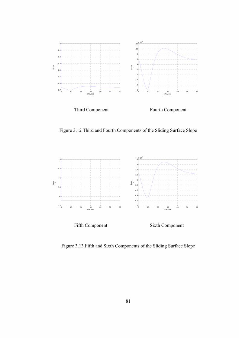
0 10 20 30 40 50 60-0.7
-0.6
-0.5
-0.4
-0.3
-0.2
-0.1
0
time, sec
Slo
pe
3
0 10 20 30 40 50 60
-6
-4
-2
0
2
4
6
8
10
12x 10-5
time, sec
Slo
pe
4
Third Component Fourth Component
Figure 3.12 Third and Fourth Components of the Sliding Surface Slope
0 10 20 30 40 50 60-2.5
-2
-1.5
-1
-0.5
0
time, sec
Slo
pe
5
0 10 20 30 40 50 60
0
0.2
0.4
0.6
0.8
1
1.2
1.4
1.6
1.8x 10⁻³
time, sec
Slo
pe
6
Fifth Component Sixth Component
Figure 3.13 Fifth and Sixth Components of the Sliding Surface Slope
81
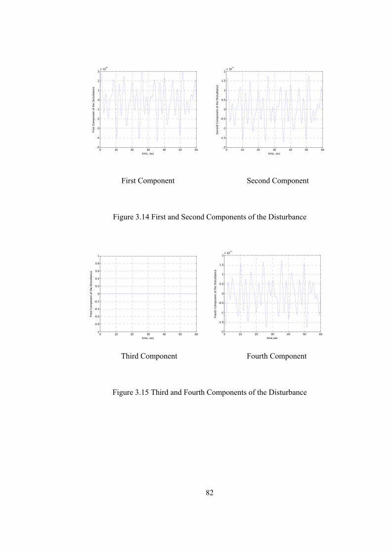
0 10 20 30 40 50 60-5
-4
-3
-2
-1
0
1
2
3x 10⁻⁸
time, sec
Firs
t Com
pone
nt o
f the
Dis
turb
ance
0 10 20 30 40 50 60
-2
-1.5
-1
-0.5
0
0.5
1
1.5
2x 10⁻⁵
time, sec
Sec
ond
Com
pone
nt o
f the
Dis
turb
ance
First Component Second Component
Figure 3.14 First and Second Components of the Disturbance
0 10 20 30 40 50 60-1
-0.8
-0.6
-0.4
-0.2
0
0.2
0.4
0.6
0.8
1
time, sec
Third
Com
pone
nt o
f the
Dis
turb
ance
0 10 20 30 40 50 60-2
-1.5
-1
-0.5
0
0.5
1
1.5
2x 10⁻⁵
time,sec
Four
th C
ompo
nent
of t
he D
istu
rban
ce
Third Component Fourth Component
Figure 3.15 Third and Fourth Components of the Disturbance
82

0 10 20 30 40 50 60-2
-1.5
-1
-0.5
0
0.5
1
1.5
2x 10⁻³
time,sec
Fifth
Com
pone
nt o
f the
Dis
turb
ance
0 10 20 30 40 50 60
-0.35
-0.3
-0.25
-0.2
-0.15
-0.1
-0.05
0
time,sec
Del
ta A
ngle
of A
ttack
(deg
)
Fifth Component Delta Angle of Attack
Figure 3.16 Fifth Component of the Disturbance and Delta Angle of Attack
83

84
3.3.2 Simulations for the Case 2: With Disturbance
This section includes the results of the simulations performed for the model
under the presence of disturbance, both for the pure SDRE method and SDRE
based SMC (ASMC) method. For comparison purposes, the results for each
state variable and control input obtained by two different methods are given
together.
The system state variables velocity, flight path angle, altitude, angle of attack
and pitch rate are presented in Figures 3.17 to 3.21 respectively while the
control inputs, elevator deflection and throttle setting are presented in Figure
3.22 and Figure 3.23.
Figures 3.24 to Figure 3.28 are given to show the variation of the parameters
specific to SMC method such as the sigma function, sliding surface slope and
the offset of sliding surface from the state space origin. The variation of the
sigma function defined in Equation (2.54) is presented Figure 3.24; the offset
of sliding surface from the state space origin is presented in Figure 3.25, the
components of the sliding surface slope are given in Figure 3.26, Figure 3.27
and Figure 3.28.
Finally, the components of the transformed disturbance or in other words the
components of the transformed state dependent disturbance vector are
presented in Figure 3.29, Figure 3.30 and Figure 3.31. The delta angle of attack
which is resulted from the wind effect and defined in Equation (3.65) is also
presented in Figure 3.31.

0 10 20 30 40 50 600
10
20
30
40
50
60
70
80
90
100
time, sec
Vel
ocity
cha
nge(
ft/se
c)
0 10 20 30 40 50 60
0
10
20
30
40
50
60
70
80
90
100
time, sec
Vel
ocity
cha
nge(
ft/se
c)
Pure SDRE (LQR) Method SDRE-based SMC Method
Figure 3.17 Velocity Change
0 10 20 30 40 50 60-0.05
0
0.05
0.1
0.15
0.2
0.25
0.3
0.35
time, sec
Flig
ht P
ath
Ang
le(d
eg)
0 10 20 30 40 50 60
-0.05
0
0.05
0.1
0.15
0.2
0.25
0.3
0.35
time, sec
Flig
ht P
ath
Ang
le(d
eg)
Pure SDRE (LQR) Method SDRE-based SMC Method
Figure 3.18 Flight Path Angle
85

0 10 20 30 40 50 60-500
0
500
1000
1500
2000
2500
time, sec
Alti
tude
cha
nge(
ft)
0 10 20 30 40 50 60
-500
0
500
1000
1500
2000
2500
time, sec
Alti
tude
cha
nge(
ft)
Pure SDRE (LQR) Method SDRE-based SMC Method
Figure 3.19 Altitude Change
0 10 20 30 40 50 601.6
1.8
2
2.2
2.4
2.6
2.8
3
3.2
time, sec
Ang
le o
f Atta
ck(d
eg)
0 10 20 30 40 50 60
1.6
1.8
2
2.2
2.4
2.6
2.8
3
time, sec
Ang
le o
f Atta
ck(d
eg)
Pure SDRE (LQR) Method SDRE-based SMC Method
Figure 3.20 Angle of Attack
86
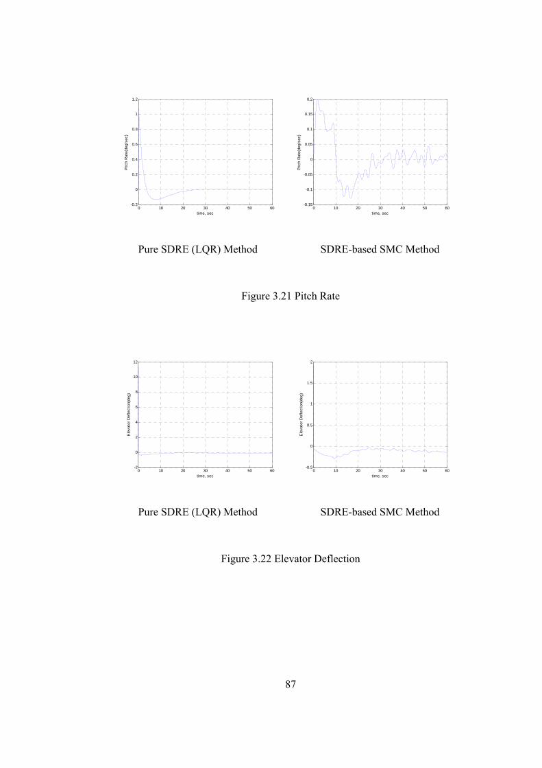
0 10 20 30 40 50 60-0.2
0
0.2
0.4
0.6
0.8
1
1.2
time, sec
Pitc
h R
ate(
deg/
sec)
0 10 20 30 40 50 60
-0.15
-0.1
-0.05
0
0.05
0.1
0.15
0.2
time, sec
Pitc
h R
ate(
deg/
sec)
Pure SDRE (LQR) Method SDRE-based SMC Method
Figure 3.21 Pitch Rate
0 10 20 30 40 50 60-2
0
2
4
6
8
10
12
time, sec
Ele
vato
r Def
lect
ion(
deg)
0 10 20 30 40 50 60
-0.5
0
0.5
1
1.5
2
time, sec
Ele
vato
r Def
lect
ion(
deg)
Pure SDRE (LQR) Method SDRE-based SMC Method
Figure 3.22 Elevator Deflection
87
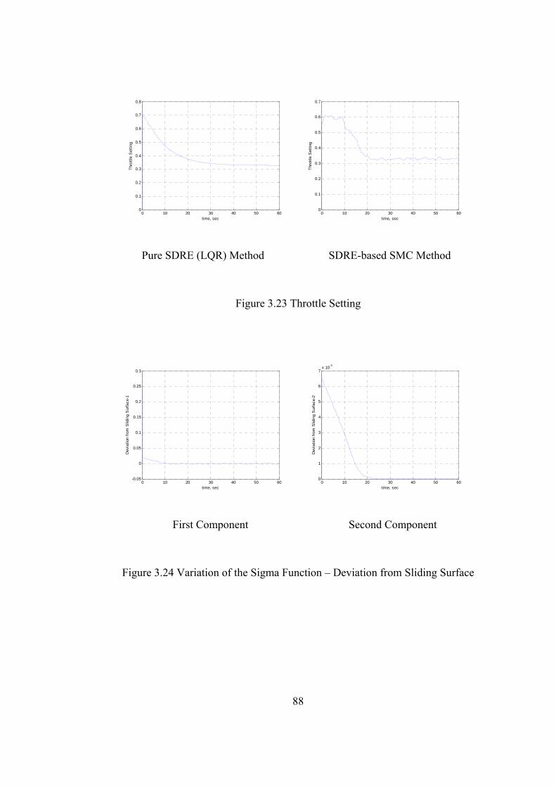
0 10 20 30 40 50 600
0.1
0.2
0.3
0.4
0.5
0.6
0.7
0.8
time, sec
Thro
ttle
Set
ting
0 10 20 30 40 50 60
0
0.1
0.2
0.3
0.4
0.5
0.6
0.7
time, sec
Thro
ttle
Set
ting
Pure SDRE (LQR) Method SDRE-based SMC Method
Figure 3.23 Throttle Setting
0 10 20 30 40 50 60-0.05
0
0.05
0.1
0.15
0.2
0.25
0.3
time, sec
Dev
iatio
n fro
m S
lidin
g S
urfa
ce-1
0 10 20 30 40 50 60
0
1
2
3
4
5
6
7x 10⁻³
time, sec
Dev
iatio
n fro
m S
lidin
g S
urfa
ce-2
First Component Second Component
Figure 3.24 Variation of the Sigma Function – Deviation from Sliding Surface
88

0 10 20 30 40 50 60-0.04
-0.035
-0.03
-0.025
-0.02
-0.015
-0.01
-0.005
0
time, sec
Firs
t Slid
ing
Sur
face
Offs
et
0 10 20 30 40 50 60-6
-5
-4
-3
-2
-1
0x 10-3
time, sec
Sec
ond
Slid
ing
Sur
face
Offs
et
First Component Second Component
Figure 3.25 First and Second Sliding Surface Offset
0 10 20 30 40 50 60-1
-0.9
-0.8
-0.7
-0.6
-0.5
-0.4
-0.3
-0.2
-0.1
0
time, sec
Slo
pe
1
0 10 20 30 40 50 60-7
-6
-5
-4
-3
-2
-1
0x 10-3
time, sec
Slo
pe
2
First Component Second Component
Figure 3.26 First and Second Components of the Sliding Surface Slope
89

0 10 20 30 40 50 60-0.8
-0.7
-0.6
-0.5
-0.4
-0.3
-0.2
-0.1
0
time, sec
Slo
pe
3
0 10 20 30 40 50 60-12
-10
-8
-6
-4
-2
0
2
4
6
8x 10⁻⁵
time, sec
Slo
pe
4
Third Component Fourth Component
Figure 3.27 Third and Fourth Components of the Sliding Surface Slope
0 10 20 30 40 50 60-2.5
-2
-1.5
-1
-0.5
0
time, sec
Slo
pe
5
0 10 20 30 40 50 60-2
0
2
4
6
8
10
12
14x 10-4
time, sec
Slo
pe
6
Fifth Component Sixth Component
Figure 3.28 Fifth and Sixth Components of the Sliding Surface Slope
90

0 10 20 30 40 50 60-1
-0.8
-0.6
-0.4
-0.2
0
0.2
0.4
0.6
0.8
1
time, sec
Firs
t Com
pone
nt o
f the
Tra
nsfo
rmed
Dis
turb
ance
0 10 20 30 40 50 60-2
-1.5
-1
-0.5
0
0.5
1
1.5
2x 10⁻⁵
time, sec
Sec
ond
Com
pone
nt o
f the
Tra
nsfo
rmed
Dis
turb
ance
First Component Second Component
Figure 3.29 First and Second Components of the Transformed Disturbance
0 10 20 30 40 50 60-2
-1.5
-1
-0.5
0
0.5
1
1.5
2x 10⁻⁵
time, sec
Third
Com
pone
nt o
f the
Tra
nsfo
rmed
Dis
turb
ance
0 10 20 30 40 50 60
-2
-1.5
-1
-0.5
0
0.5
1
1.5
2x 10⁻³
time, sec
Four
th C
ompo
nent
of t
he T
rans
form
ed D
istu
rban
ce
Third Component Fourth Component
Figure 3.30 Third and Fourth Components of the Transformed Disturbance
91

0 10 20 30 40 50 60-1.5
-1
-0.5
0
0.5
1
1.5
2x 10⁻⁶
time, sec
Fifth
Com
pone
nt o
f the
Tra
nsfo
rmed
Dis
turb
ance
0 10 20 30 40 50 60-0.35
-0.3
-0.25
-0.2
-0.15
-0.1
-0.05
0
time,sec
Del
ta A
ngle
of A
ttack
(deg
)
Fifth Component Delta Angle of Attack
Figure 3.31 Fifth Component of the Transformed Disturbance and Delta Angle
of Attack
As it can be seen from above figures, simulations have been performed for four
cases;
• Pure SDRE (LQR) method applied alone for the nominal model,
• Pure SDRE (LQR) method applied for the model under the presence of
disturbance,
• SDRE (LQR) method combined with SMC technique for the nominal
model,
• SDRE (LQR) method combined with SMC technique for the model
under the presence of disturbance.
It is possible to tune the reaching time to sliding surface, i.e., time needed to
reach the steady state conditions and control system performance (values of
system state variables and control inputs) by changing the values of K, Q11 and
Q22.
92

93
The proper K is to be selected such that the sliding surface is reached in a
minimum time and disturbance rejection is maintained simultaneously without
destroying the system stability. On the other hand, appropriate Q11 and Q22
matrices should be selected to provide both optimal control effort and feasible
controlled system response. For instance, the physical limitations in the state
variables such as Angle of Attack and the physical limitations in the control
inputs such as the elevator deflection have to be respected. These are the
challenging goals of the controller design.
Another point is the effect of using MATLAB® (The MathWorks Inc., 2004)
“ode” function. The use of this function very often leads to some perturbations
on the system response. One way to handle this problem is to select the
integration time step smaller to prevent any numerical error. However, using
smaller integration time step increases the simulation time.
It is noted that the relation between integration time step and chattering
frequency should be carefully analyzed such that chattering frequency can be
caught by integration time step. Since incorrect selection of integration time
step may result with erroneous simulation results. In this study, by trial and
error method, it is observed that the selected integration time step is sufficient
enough to catch the chattering frequency. Here are four examples from case
study simulation results which are performed by the use “sign” function to
emphasise the effects of incorrect integration time step selection on chattering
frequency and results consequently. Control inputs in the case study, elevator
deflection and throttle setting are presented for four different integration time
step selections. The integration time step is 0.1 for the result presented in
Figure 3.32, 0.01 for the result presented in Figure 3.33, 0.001 for the result
presented in Figure 3.34 and 0.5 for the result presented in Figure 3.35.

It is concluded that the chattering cannot be observed correctly for the cases
given in Figure 3.32 and Figure3.35 while it can be observed correctly for the
cases given in Figure 3.33 and Figure 3.34. Therefore, the values 0.01 and 0.01
are determined as good candidates for the integration time step selection.
However, the required time for the simulation increases significantly if the
integration time step is selected 0.001 instead of 0.01 and a few numerical
errors are observed as seen in Figure 3.34. In summary, 0.01 is selected as an
integration time step value for the case study simulations given in section 3.3.1
and 3.3.2.
0.8
0 10 20 30 40 50 60-0.5
0
0.5
1
1.5
2
time, sn
Ele
vato
r Def
lect
ion(
deg)
94
Elevator Deflection Throttle Setting
Figure 3.32 Control Inputs for Integration Time Step is 0.1
0 10 20 30 40 50 600
0.1
0.2
0.3
0.4
0.5
0.6
0.7
Thro
ttle
Set
tling
time, sn
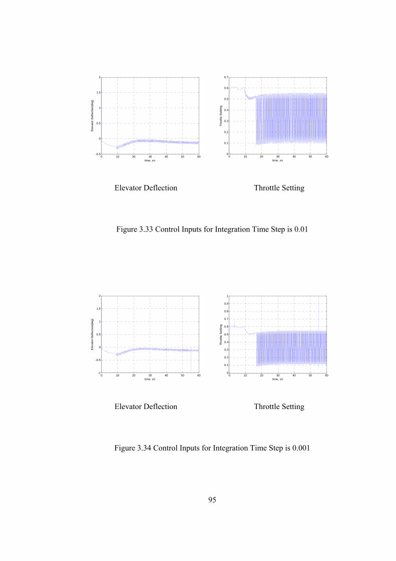
0.7
0 10 20 30 40 50 60-0.5
0
0.5
1
1.5
2
time, sn
Ele
vato
r Def
lect
ion(
deg)
95
Elevator Deflection Throttle Setting
Figure 3.33 Control Inputs for Integration Time Step is 0.01
Elevator Deflection Throttle Setting
Figure 3.34 Control Inputs for Integration Time Step is 0.001
0 10 20 30 40 50 600
0.1
0.2
0.3
0.4
0.5
0.6
0.7
0.8
0.9
1
time, sn
Thro
ttle
Set
tling
0 10 20 30 40 50 60-1
-0.5
0
0.5
1
1.5
2
time, sn
Ele
vato
r Def
lect
ion(
deg)
0 10 20 30 40 50 600
0.1
0.2
0.3
0.4
0.5
0.6
Thro
ttle
Set
tling
time, sn

0 10 20 30 40 50 600
0.1
0.2
0.3
0.4
0.5
0.6
0.7
0.8
0.9
1
time, sn
Thro
ttle
Set
tling
0 10 20 30 40 50 60-0.5
0
0.5
1
1.5
2
time, sn
Ele
vato
r Def
lect
ion(
deg)
Elevator Deflection Throttle Setting
Figure 3.35 Control Inputs for Integration Time Step is 0.5
The sliding surface slope and the offset of sliding surface from the state space
origin are changing with the variations in system state variables and become
constant after system state variables had reached their steady state values as
expected. This showed that the sliding surface slope and the offset of sliding
surface from the state space origin have been adapted for the changes in system
state variables (adaptive manner) and the determination of sliding surface slope
is optimally selected for the given Q11 and Q22 matrices (optimality manner).
As a summary, proposed SMC is capable of leading the non-linear system up
to its desired equilibrium points even under the presence of disturbance.
96

97
CHAPTER
4. CONCLUSIONS
4.1 Summary The aim of this thesis study is to design a sliding mode controller for a linearly
actuated non-linear system. A longitudinal model of a generic hypersonic air
vehicle is used to show the performance of the proposed controller. The
problem can be summarised as tracking the velocity and altitude commands via
controlling the deflection of the elevator and thrust by means of a throttle
setting both for the nominal model and for the model under the presence of
disturbance.
In the first part of the study, brief information about the general SMC design
principles and detailed description of the SMC design methodology proposed
in this study are given. Then the hypersonic air vehicle model which was
studied previously in some papers and the differential equations of the system
are presented. In the next chapter, the proposed SMC is derived for this
hypersonic air vehicle model based on the principles explained in section 2.2.
Finally, simulations are performed on MATLAB® for four cases to observe the
controller performance.

98
4.2 Major Conclusions
The main contribution of this study is to design sliding mode control for a non-
linear system by means of solving SDRE’s online during the control process
and designing the sliding surface correspondingly. This approach both adds an
adaptive manner to the classical SMC while combining it with the optimal
sliding surface parameter selection.
Adaptive manner includes only the automatic adaptation of the sliding surface
by determining the sliding surface slop and the offset of sliding surface from
the state space while system state variables are changing.
The method developed in this thesis study is applied to a non-linear flight
dynamics which was studied in [10] as well. In [10], another adaptive sliding
mode control design approach is suggested. This method is based on the Input-
Output linearization technique which requires additional computations.
Nonetheless, linearization is made over the nominal model while the original
system is still non-linear. This means that the system that was worked on
through the controller design phase includes certain amount of approximations
beyond linearization.
On the other hand, in this study, a different approach to the SMC is presented
which is combined with SDRE. First of all, the system is not linearised to
design the sliding mode controller, in other words, the non-linearity of the
original system is kept during the controller design phase. Secondly the method
computes the required control in a systematic way since it uses the well-known
linear quadratic regulator (LQR) algorithms which are available in many
existing software.

99
Not only the practical property of the suggested method in this study, but also
the simulation results have some positive features compared to the results of
[10]. For instance, in [10], only either velocity or altitude commands are given
while in this study, both velocity and altitude commands are given to the same
plant and these commands are tracked successfully.
In addition to the above features, the methodology proposed in this study
includes some features which can be assumed as relatively new or in other
words, which are not common in the literature such as the combining the
SDRE technique with the SMC approach and adding the adaptable sliding
surface offset term to the definition of the sliding surface.
It is obviously seen from figures that the combined control methodology
(ASMC or SMC combined with SDRE) had a basic advantage on the
simulations made for nominal model and for the case under the presence of
disturbance when compared with the SDRE method. There is a relatively large
control effort need for the first method when the performances are compared
for both cases. It is a natural outcome of the SMC design technique since SMC
is expected to be robust against the disturbances in the input channel (matched
disturbances) while SDRE based controller must suppress both matched and
unmatched disturbances.
The second reason of this improvement in controller performance is the use of
ASMC instead of classic SMC since pure SMC presents drawbacks that
include large control authority requirements and chattering. However, the
control gains cannot be chosen arbitrary large due to practical considerations
such as reaching control surface deflection limits.

100
Furthermore, control chattering is undesirable in practice because it involves
high control activity and may excite high-frequency un-modelled dynamics.
These drawbacks are addressed by the addition of adaptation capability to
SMC.

101
4.3 Recommendations for Future Work
As an extension of this thesis study, performance of the proposed ASMC
(SDRE combined SMC) can be compared with,
- the SMC designed for the model linearised about the initial and/or final
conditions,
- the SMC designed with constant sliding surface parameters, i.e. sliding
surface slope and the offset of sliding surface from the state space,
- the pure SDRE method proposed in this study for the cases when there
is disturbance with non-zero mean values,
- the pure SDRE method proposed in this study when there are variations
in the parameters.
102
REFERENCES [1] V. I. Utkin, 1977, Variable Structure Systems with Sliding Modes, IEEE Transactions on Automatic Control, 22, pp. 212-222. [2] C. Edwards, 1998, S. K. Spurgeon, Sliding Mode Control: Theory and Applications, Taylor and Francis Ltd. [3] R.A. De Carlo, S. H. Zak, and G. P. Matthews, 1988, Variable Structure Control of Nonlinear Multivariable Systems: A Tutorial, Proceedings of the IEEE, 76, pp. 212-232. [4] V. I. Utkin, 1992, Sliding Modes in Control and Optimization, Berlin: Springer-Verlag. [5] S. J. Dodds and A. G. Luk’yanov, 1996, Sliding Mode Block Control of Uncertain Nonlinear Plants, 13th IFAC Triennial World Congress, pp. 241-146. [6] H. Sira Ramirez, 1993, A Dynamical Variable Structure Control Strategy in Asymptotic Output Tracking Problems, IEEE Transactions on Automatic Control, 38, pp. 615-620. [7] R. Hirschorn, 2003, Sliding Mode Control Design for Nonlinear Systems, Canada Natural Sciences and Engineering Research Council Report. [8] Y. Niu, J. Lam, X. Wang and D.W.C Ho, 2004, Observer-based Sliding Mode Control for Nonlinear State-delayed Systems, International Journal of Systems Science, 35, pp. 139-150.

103
[9] K. D. Young, V. I. Utkin, Ü. Özgüner, 1999, A Control Engineer’s Guide to Sliding Mode Control, IEEE Transactions on Control Systems Technology, 7, pp. 328-342. [10] H. Xu, P. A. Ioannou and M. Mirmirani, Adaptive Sliding Mode Control Design for A Hypersonic Flight Vehicle, Journal of Guidance, Control, and Dynamics 2004, vol.27 no.5, pp. 829-838. [11] J.-J. Slotine, and L. Weiping, 1991, Applied Nonlinear Control, Prentice Hall. [12] C. I. Marrison and R. F. Stengel, , 1998, Design of Robust Control System For a Hypersonic Aircraft, Journal of Guidance, Control, and Dynamics, Vol. 21, No. 1. [13] Q. Wang and R. F. Stengel, 2000, Robust Nonlinear Control of a Hypersonic Aircraft, J. of Guidance, Control and Dynamics, Vol. 23, No. 4. [14] ADEX, S.L., 2007, Adaptive Predictive Expert Control, http://www.adexcop.com, 30th of October 2009. [15] Mracek C. P. and Cloutier J. R., 1998, Control Designs for the Nonlinear Benchmark Problem via the State-Dependent Riccati Equation Method, International Journal of Robust And Nonlinear Control, Int. J. Robust Nonlinear Control Vol. 8, pp. 401-433. [16] M Qian, 1997, Sliding Mode Controller Design for ABS System, M.Sc. Thesis, Electrical and Computer Engineering Department, College of Natural Resources, Virginia Tech. [17] Utkin, V.I. and Young, K.-K.D, 1978, Methods for Constructing Discontinuity Planes in Multidimensional Variable Structure Systems, Automation and Remote Control Vol. 39, pp. 1466-1470.

104
[18] Banks, S.P., Salamcı, M.U. and Özgören, M.K., 1999, On the Global Stabilization of Nonlinear Systems via Switching Manifolds, Turk J Elec Engin, Vol.7, No.1-3 © TUBITAK. [19] İtik M., Salamcı, M.U. and Ülker F. D., 2005, Vibration Suppression of An Elastic Beam via Sliding Mode Control, E. Inan and A. Kırış (eds), Vibration Problems ICOVP 2005, pp. 237–242 © 2007 Springer. [20] Itik M., Salamcı, M.U., Ülker F. D. and Yaman, Y., 2005, Active Vibration Suppression of a Flexible Beam via Sliding Mode and H∞ Control, Decision and Control, 2005 and 2005 European Control Conference, pp. 1240- 1245. [21] Itik M., Salamcı, M.U. and Banks, S.P., 2009, Optimal Control Of Drug Therapy In Cancer Treatment, Nonlinear Analysis: Theory, Methods & Applications, in Press. [22] Tombul G. S., Banks S. P.,and Akturk N., 2009, Sliding Mode Control For A Class Of Non-Affine Nonlinear Systems , Nonlinear Analysis: Theory, Methods & Applications, in Press, Corrected Proof. [23] Salamcı, M.U., Özgören, M.K. and Banks, S.P., 2000, Sliding Mode Control with Optimal Sliding Surfaces for Missile Autopilot Design, Journal of Guidance, Control, And Dynamics, Vol. 23, No. 4. [24] Salamcı, M.U. and Gökbilen B., 2007, SDRE Missile Autopilot Design using Sliding Mode Control with Moving Sliding Surfaces, 17th IFAC Symposium on Automatic Control in Aerospace. [25] Salamcı, M.U. and Gökbilen B., 2006, Doğrusal Olmayan Sistemlerin Zamanla Değişen Doğrusal Yüzey Kullanılarak Kayan Kipli Kontrolü ve Uygulamaları, M.Sc. Thesis, Mechanical Engineering Department, Gazi University.

105
[26] Salamcı, M.U. and Gökbilen B., 2006, Alçak Yörüngeli Küçük Uyduların Doğrusal Olmayan Konum Kontrolü, Otomatik Kontrol Ulusal Toplantısı, TOK’06, TOBB Ekonomi ve Teknoloji Üniversitesi. [27] Salamcı, M.U. and Tombul G. S., 2006, Sliding Mode Control Design with Time Varying Sliding Surfaces for a Class of Nonlinear Systems, Proceedings of the 2006 IEEE, International Conference on Control Applications. [28] Çimen T., 2008, State-Dependent Riccati Equation (SDRE) Control: A Survey, Proceedings of the 17th World Congress, The International Federation of Automatic Control. [29] Wang Y.-P. and Sinha A., 1998, Adaptive Sliding Mode Control Algorithm for a Microgravity Isolation System, Acta Astronautica, Vol. 43, No. 7-8, pp. 377-384. [30] Yau H.-T. and Yan J.-J., 2008, Adaptive Sliding Mode Control of a High-Precision Ball-Screw-Driven Stage, Nonlinear Analysis: Real World Applications. [31] Huang Y.-J., Kuo T.-C. and Chang S.-H., 2008, Adaptive Sliding-Mode Control for Nonlinear Systems With Uncertain Parameters, IEEE Transactions On Systems, Man, And Cybernetics - Part B: Cybernetics, Vol. 38, No. 2. [32] Huang A.-C. and Chen Y.-C., 2004, Adaptive Sliding Control for Single-Link Flexible-Joint Robot With Mismatched Uncertainties, IEEE Transactions on Control Systems Technology, Vol. 12, No. 5. [33] Yoerger D. R. and Slotine J.-J. E., 1991, Adaptive Sliding Control of an Experimental Underwater Vehicle, Proceedings of the 1991 IEEE International Conference on Robotics and Automation. [34] Wai R.-J., 2000, Adaptive Sliding Mode Control for Induction Servomotor Drive, IEE Pwc.-Cleclr. Power Appl,, Vol. 147, No. 6.

106
[35] D Zhou, Mu, C. and Xu W., 1999, Adaptive Sliding-Mode Guidance of a Homing Missile, Journal of Guidance, Control, and Dynamics, Vol. 22, No. 4. [36] Lee K. W., Nambisan P. R. And Singh S. N., 2008, Adaptive Variable Structure Control of Aircraft with an Unknown High-Frequency Gain Matrix, Journal of Guidance, Control, and Dynamics, Vol. 31, No. 1. [37] H.K. Khalil, 1996, Nonlinear Systems, New Jersey: Printice-Hall. [38] Cloutier J. R., 1997, State-Dependent Riccati Equation Techniques: An Overview, Proceedings of the American Control Conference Albuquerque. [39] Erdem E. B. and Alleyne A. G., 2004, Design of a Class of Nonlinear Controllers via State Dependent Riccati Equations, IEEE Transactions on Control Systems Technology, Vol. 12, No. 1. [40] Diong B. M., 2004, Sliding Mode Control Design for a Class of Systems With Non-Matching Nonlinearities and Disturbances, International Journal of Systems Science, Volume 35, Number 8, 10 July 2004, pp. 445–455. [41] Kim K.-S., Park Y. and Oh S.-H., 2000, Designing Robust Sliding Hyperplanes for Parametric Uncertain Systems: a Riccati Approach, Automatica No.36, pp. 1041 - 1048. [42] Spurgeon S. K. and Lu X. Y., 1997, Output Tracking Using Dynamic Sliding Mode Techniques, International Journal of Robust and Nonlinear Control, Vol. 7, pp. 407 – 427. [43] Chou C.-H. and Cheng C.-C., 2001, Design of Adaptive Variable Structure Controllers for Perturbed Time-Varying State Delay Systems, Journal of the Franklin Institute, Vol. 338, pp. 35 – 46.
107
APPENDIX A MAIN SCRIPT
clc;clear;
tic
global t_inc k tspan xd ud
epsilonbig=1e-6;
epsilonsml=1e-9;
xd=[15160;
0;
112000;
2.00042687579048*pi/180;
0];
ud=[-0.11534710655337*pi/180;0.32921240198018];
x0(1)=15060;
x0(2)=(0+epsilonsml)*pi/180;
x0(3)=110000;
x0(4)=1.79*pi/180;
x0(5)=(0+epsilonsml)*pi/180;

108
x0(1)=(0)/(15060);
x0(3)=(0)/(110000);
xd(1)=(100)/(15060);
xd(3)=(2000)/(110000);
format long;
xtilde=x0;
t_start=0; % Starting time
t_final=60; % Final time
t_inc=1e-2; % Time increment value
tspan=[t_start:t_inc:t_final];
k=[-0.002 -0.0004];
k=diag(k);% factor that maintains the sliding direction is shifted to zero
%-------------------------------------------------------------------------%
% ODE Solver
%-------------------------------------------------------------------------%
display('Solution is running');
[x,Ucon,sigma,KY,h2,d2]=ode5x(@control,tspan,xtilde);
result(1).x1=(15060*(x(:,1)+1))-15060;
result(1).x2=180/pi*(x(:,2));
result(1).x3=(110000*(x(:,3)+1))-110000;
result(1).x4=180/pi*(x(:,4));
result(1).x5=180/pi*(x(:,5));
result(1).U1=180/pi*(Ucon(1,:));
result(1).U2=(Ucon(2,:));
result(1).sigma1=sigma(1,:);
result(1).sigma2=sigma(2,:);
109
hh2=cell2mat(h2);
result(1).h21=hh2(1,:);
result(1).h22=hh2(2,:);
dd2=cell2mat(d2);
result(1).d21=dd2(1,:);
result(1).d22=dd2(2,:);
result(1).time=tspan;
% C hesaplama ve plot
for i=1:6
for j=1:length(KY)
C(i,j)=KY{j}(i);
end
figure(i+13); plot (tspan,C(i,:)),xlabel('time, sn'),ylabel({'Slope ', i}); grid on;
end
%%
figure (1); plot (result(1).time,result(1).x1),xlabel('time, sn'),ylabel('Velocity
change(ft/sec)'); grid on;
figure (2); plot (result(1).time,result(1).x2),xlabel('time, sn'),ylabel('Flight Path
Angle(deg)'); grid on;
figure (3); plot (result(1).time,result(1).x3),xlabel('time, sn'),ylabel('Altitude
change(ft)'); grid on;
figure (4); plot (result(1).time,result(1).x4),xlabel('time, sn'),ylabel('Angle of
Attack(deg)'); grid on;
figure (5); plot (result(1).time,result(1).x5),xlabel('time, sn'),ylabel('Pitch
Rate(deg/sec)'); grid on;
figure (6); plot (result(1).time,result(1).U1),xlabel('time, sn'),ylabel('Elevator
Deflection(deg)'); grid on;

110
figure (7); plot (result(1).time,result(1).U2),xlabel('time, sn'),ylabel('Throttle Setting');
grid on;
figure (8); plot (result(1).time,result(1).sigma1),xlabel('time, sn'),ylabel('First Sliding
Surface'); grid on;
figure (9); plot (result(1).time,result(1).sigma2),xlabel('time, sn'),ylabel('Second
Sliding Surface'); grid on;
figure (10); plot (result(1).time,result(1).h21),xlabel('time, sn'),ylabel('First Sliding
Surface Offset'); grid on;
figure (11); plot (result(1).time,result(1).h22),xlabel('time, sn'),ylabel('Second Sliding
Surface Offset'); grid on;
figure (12); plot (result(1).time,result(1).d21),xlabel('time, sn'),ylabel('First
Component of the Disturbance'); grid on;
figure (13); plot (result(1).time,result(1).d22),xlabel('time, sn'),ylabel('Second
Component of the Disturbance'); grid on;
toc
display('Process Finished.');

111
APPENDIX B
FUNCTION FOR DESIGNING CONTROLLER function [phitildedot,Ucon,sigma,C,Tr,h2,d2]=control(t,phitilde,Cp,Tp,h2p)
global t_inc xd ud
epsilonbig=1e-6;
epsilonsml=1e-9;
phid=xd;
%% Transformation of the system to Canonical Form
[A,B,F,D] = sistem(phitilde);
Tr=T_find(A,B);
if (t==0)
Told=Tr;
else
Told=Tp;
end
Tp=Told;
Tdot=(Tr-Told)/t_inc;

112
[Tr,Abar11,Abar12,Abar21,Abar22,Bbar2]=T_find(A,B,Tdot);
contr=ctrb(Abar11,Abar12);
% rank(contr);
% if(rank(contr)==length(Abar11)) display('Controllable System');
%
% else display('System is Uncontrollable !!!!!!!!!!!!!!!!!');
% end
% ranks=rank(sym(contr));
% if(ranks==length(Abar11)) display('Controllable System');
%
% else display('System is Uncontrollable !!!!!!!!!!!!!!!!!');
% end
%% Determination of Sliding Surface Slope and the Offset of the Sliding Surface
%% Surface
[C h2]=c_find(Abar11,Abar12,phitilde,F,Tr);
if (t==0)
Cold=C;
h2old=h2;
else
Cold=Cp;
h2old=h2p;
end
% Cp=Cold;
% h2p=h2old;
113
Cdot=(C-Cold)/t_inc; % Time derivative of C matrix Cdot = d(T)/dt
h2dot=(h2-h2old)/t_inc;
%% Sliding Mode Control Design
z=Tr*phitilde;
f=Tr*F;
f1=f(1:3,1);
f2=f(4:5,1);
z1=z(1:3,1);
z2=z(4:5,1);
sigma=C*z1+z2-h2;
%% Disturbance Injection
Im=-0.25*pi/180;
If=0.025*pi/180*(sin(t)+sin((3^0.5)*t)+sin((5^0.5)*t))/3;
D(1)=D(1)*((2*0.645*Im*If)+(0.645*If^2)+(0.0043378*If));
D(2)=D(2)*(0.6203*If);
D(5)=D(5)*((-0.035)*2*Im*If-(0.035*If^2)+0.036617*If);
%% Relation between SMC Gain and Disturbance
g=Tr*D;
d1=g(1:3,1);
d2=g(4:5,1);
114
% Equivalent Control
ueq=-inv(Bbar2)*(Cdot*z1+C*(Abar11*z1+Abar12*z2+f1)+...
(Abar21*z1+Abar22*z2+f2)-h2dot);
% High Frequency control signal
global k;
uhf=inv(Bbar2)*k*tanh(1000*sigma);...smooth;
Ucon=ueq+uhf;
%% Physical Limitations on Control Inputs
if Ucon(2,:)<0;
Ucon(2,:)=0;
end
if Ucon(2,:)>1;
Ucon(2,:)=1;
end
if (180/pi*Ucon(1,:))>1;
Ucon(1,:)=1*pi/180;
end
%% Differential Equation
phitildedot=A*phitilde+B*Ucon+F+D;

115
APPENDIX C
FUNCTION FOR CONSTRUCTING SYSTEM AND CONTROL MATRICES function [A,B,F,D]=sistem(x0)
%%--------------------------------------------------------------------------
% This function is to describe the dynamics of the system without an unbalanced
% mass. The only external effect is gravity.
% dx/dt = A(x)*x + B(x,u)*u + F;
% global
epsilonsml=1e-9;
%% Initialisation of the matrices.
%--------------------------------------------------------------------------
A=zeros(5,5);
B=zeros(5,2);
F=zeros(5,1);
% ---------------------------------
% p ve ne degerlerinin belirlenmesi
% ---------------------------------
p=0;
n=0.02576;
% % ---------------------------------
Im=-0.25*pi/180;
116
%%%%%%%%%%
V=15060*(1+x0(1));
gamma=x0(2);
h=110000*(1+x0(3));
alpha=x0(4);
q=x0(5);
%%%%%%%%%%
m=9375;
Iyy=7*10^6;
S=3603;
cbar=80;
ce=0.0292;
mu=1.39*10^16;
RE=20903500;
ro=0.24325*1e-4;
r=h+RE;
a11=-(15060)*(1/15060)*(((ro*V*S/(m))*0.003772));
a12=-(1/15060)*(mu*sin(gamma)/(r^2*(gamma+epsilonsml)));
a14=-(1/15060)*((ro*V^2*S/(2*m))*(0.6450*alpha+0.0043378));
b12=(1/15060)*(((ro*V^2*S/(2*m))*n*cos(alpha)));
%
a21=-(15060)*(((mu-V^2*r)*cos(gamma))/(V^2*r^2));
a24=((ro*V*S/(2*m))*0.6203);
b22=((ro*V*S/(2*m))*n*sin(alpha));
a32=(1/110000)*(V*(sin(gamma)/(gamma+epsilonsml)));
a41=(15060)*(((mu-V^2*r)*cos(gamma))/(V^2*r^2));
a44=-((ro*V*S/(2*m))*0.6203);

117
a45=1;
b42=-((ro*V*S/(2*m))*n*sin(alpha));
a51=(15060)*((ro*V*S)*cbar*(5.3261*10^-6)/Iyy);
a54=(0.5*(ro*V^2*S)*cbar*(-ce-
0.035*alpha+0.036617)/Iyy)+(0.25*(ro*V*S*q)*(cbar^2)*(-
6.796*alpha+0.3015)/Iyy);
a55=(0.25*(ro*V*S)*(cbar^2)*(-0.2289)/Iyy);
b51=(0.5*(ro*V^2*S)*cbar*ce/Iyy);
f1=(-(((ro*V*S/(m))*0.003772)))-
(1/15060)*(((ro*V^2*S/(2*m))*(0.645*Im^2+0.0043378*Im)));
f2=(-(15060)*(((mu-
V^2*r)*cos(gamma))/(V^2*r^2)))+(ro*V*S/(2*m))*(0.6203*Im);
f3=0;
f4=(15060)*((((mu-V^2*r)*cos(gamma))/(V^2*r^2)));
f5=((15060)*((ro*V*S)*cbar*(5.3261*10^-6)/Iyy))+((0.5*(ro*V^2*S*cbar)*(-
0.035*Im^2+0.036617*Im)/Iyy));
d1=-(1/15060)*(ro*V^2*S/(2*m));
d2=(ro*V*S/(2*m));
d3=0;
d4=0;
d5=(0.5*(ro*V^2*S*cbar/Iyy));
%%%%%%%%%%%%
A=[a11 a12 0 a14 0;a21 0 0 a24 0;0 a32 0 0 0;a41 0 0 a44 a45;a51 0 0 a54 a55];
B=[0 b12;0 b22;0 0;0 b42;b51 0];
F=[f1;f2;f3;f4;f5];
D=[d1;d2;d3;d4;d5];

118
APPENDIX D
FUNCTION FOR TRANSFORMING THE SYSTEM TO CANONICAL FORM function [Tr,varargout]=T_find(A,B,varargin)
% Transformation matrix for suitable canonical form. [0;B2]
% Burak DURMAZ
%--------------------------------------------------------------------------%
% Establish the size of the input distribution matrix
%--------------------------------------------------------------------------%
[nn,mm]=size(B);
%--------------------------------------------------------------------------%
% Perform QR decomposition on the input distribution matrix
%--------------------------------------------------------------------------%
[Tr temp]=qr(B);
Tr=Tr';
Tr=[Tr(mm+1:nn,:);Tr(1:mm,:)];
if (nargout>1)
if(nargin>3)
Tdot=varargin{1};
else
Tdot=zeros(nn);
end

119
%--------------------------------------------------------------------------%
% Obtain (Areg,Breg); regular form description
%--------------------------------------------------------------------------%
Areg=Tr*A*Tr'+Tdot*Tr';
Breg=Tr*B;
%--------------------------------------------------------------------------%
% Obtain matrix sub-blocks for sliding mode controller design
%--------------------------------------------------------------------------%
A11 = Areg(1:nn-mm,1:nn-mm);
A12 = Areg(1:nn-mm,nn-mm+1:nn);
A21 = Areg(nn-mm+1:nn,1:nn-mm);
A22 = Areg(nn-mm+1:nn,nn-mm+1:nn);
B2 = Breg(nn-mm+1:nn,1:mm);
varargout{1}=A11;
varargout{2}=A12;
varargout{3}=A21;
varargout{4}=A22;
varargout{5}=B2;
end

120
APPENDIX E FUNCTION FOR SLIDING SURFACE SLOPE DETERMINATION function [S,varargout]=c_find(A11,A12,phitilde,F,Tr,varargin)
% Sliding Hyperplane Design with LQR method.
% Burak DURMAZ
global t_inc xd ud
L=zeros(5,2);
[nn,mm]=size(L);
Q=diag([10 1 1 0.2 1])*1e2*3;
Qt=Tr*Q*Tr';
Q11 = Qt(1:nn-mm,1:nn-mm);
Q12 = Qt(1:nn-mm,nn-mm+1:nn);
Q21 = Qt(nn-mm+1:nn,1:nn-mm);
Q22 = Qt(nn-mm+1:nn,nn-mm+1:nn);
% Form reduced order system description and associated weighting matrix
Qhat=Q11;...-Q12*inv(Q22)*Q21;
Ahat=A11;...-A12*inv(Q22)*Q21;
A=Ahat;
B=A12;
Q=Qhat;
R=Q22;

121
% Solve the LQR problem
[K,S,E]=lqr(A,B,Q,R);
z=Tr*phitilde;
f=Tr*F;
r=Tr*xd;
f1=f(1:3,1);
f2=f(4:5,1);
z1=z(1:3,1);
z2=z(4:5,1);
r1=r(1:3,1);
r2=r(4:5,1);
G=B*inv(R)*B';
psi=inv(-A'+S*G)*((-Q*r1)+S*(f1+B*r2));
slope=inv(R)*(B')*S;
h2=r2-inv(R)*(B')*psi;
% Obtain the switching function matrix in terms of the original coordinates
S=slope;
varargout{1}=h2;

122
APPENDIX F BRIEF USER MANUAL
The “Mainscript” is the main baseline of this study’s software coding as it can
be understood from its name. It is enough for the user to run this program to
see all the results. Since all other functions are automatically called by this
main script. The initial and desired values which are related with system state
variables and control inputs can be adjusted in main script also. Additional, the
gain of the sliding mode controller, k and simulation time adjustments have
been changed in main script.
To adjust the weighting matrices Q and R, user can set the Q11 for adjusting Q
and Q22 for adjusting R in function “c_find” given in E.
System matrices f and B are constructed in function “sistem” given in C. and all the
constant system parameters are also embedded inside this function.
The function “T_find” given in D. is used to transform the system in to the
canonical form in order to design the SMC via the proposed method.
The most important function is called “control”, given in B. and it determines
the SMC with the help of other functions.

123
CURRICULUM VITAE
PERSONAL INFORMATION Surname, Name: Durmaz, Burak Nationality: Turkish (TC) Date and Place of Birth: 1 January 1983, Isparta Marital Status: Single Phone: + 90 312 811 26 11 Email: [email protected] EDUCATION Degree Institution Year of Graduation Double Major Program Gazi University, Electrical and Electronics 2006
Engineering Department BS Gazi University, Mechanical 2005
Engineering Department High School Isparta Süleyman Demirel Fen Lisesi, 2001
Isparta WORK EXPERIENCE Year Place Enrolment 2006-Present Turkish Aerospace Industries Systems Engineer , Inc. (TAI) FOREIGN LANGUAGES Advanced English, Basic German PUBLICATIONS 1. Burak D., Mine Alemdaroğlu T., Pınar E. “Tusaş Uçuş/Sistem Emniyeti Faaliyetlerinin Değerlendirilmesi ve Geleceğe Yönelik Öneriler”, Savunma Sanayii Müsteşarlığı (SSM) III. Kalite Kurultayı (2008) HOBBIES Swimming, History, Politics, Movies, Dance, Football, Travel


![Robust Fuzzy-Second Order Sliding Mode based …thesai.org/...Robust_Fuzzy_Second_Order_Sliding_Mode_based...Con… · Robust Fuzzy-Second Order Sliding Mode based ... [3]. Sliding-mode](https://img.dokumen.tips/doc/110x75/5b7a16407f8b9a483c8b5dce/robust-fuzzy-second-order-sliding-mode-based-robust-fuzzy-second-order-sliding.jpg)