Embed Size (px)
Citation preview

SIMPLIFIED MULTIUSER DETECTION FOR CDMA
SYSTEMS
a dissertation
submitted to the department of electrical engineering
and the committee on graduate studies
of stanford university
in partial fulfillment of the requirements
for the degree of
doctor of philosophy
Zartash Afzal Uzmi
September 2002

c© Copyright by Zartash Afzal Uzmi 2003
All Rights Reserved
ii

I certify that I have read this dissertation and that in
my opinion it is fully adequate, in scope and quality, as
a dissertation for the degree of Doctor of Philosophy.
G. L. Tyler(Principal Adviser)
I certify that I have read this dissertation and that in
my opinion it is fully adequate, in scope and quality, as
a dissertation for the degree of Doctor of Philosophy.
M. J. Narasimha
I certify that I have read this dissertation and that in
my opinion it is fully adequate, in scope and quality, as
a dissertation for the degree of Doctor of Philosophy.
M. G. Baker
Approved for the University Committee on Graduate
Studies:
iii

Abstract
The capacity of Direct Sequence Code Division Multiple Access (DS-CDMA) systems
is limited by multiple access interference (MAI) instead of thermal noise. Commercial
CDMA systems, such as the ones based on the IS-95 standard, regard MAI as additive
noise and employ matched filter detectors. This technique limits the number of users
that can be supported in a DS-CDMA system to less than 10% of the spreading gain.
Moreover, the bit error rates for individual users degrade rapidly with an increase in
the number of users.
A new sub-symbol based multiuser detection technique addresses the two ma-
jor concerns in DS-CDMA systems: high bit error rates and low system capacity.
The two filters in traditional multiuser detectors—a code-matched and a multiuser
linear filter—are designed independently, resulting in an increase in system complex-
ity due to asynchronous operation. Multiuser detection based on sub-symbols is a
joint optimization of the code-matched filter and the linear multiuser detection filter.
This design approach drastically reduces the implementation complexity while asymp-
totically approaching the ideal performance exhibited by the zero-forcing multiuser
detector.
In the sub-symbol scheme, data symbols of users are partitioned into sub-symbols
such that the resulting sub-symbols from different users are time-aligned at the re-
ceiver. Simplified optimal linear filters operate in each sub-symbol interval, and the
filtered outputs are processed using various diversity combining algorithms. Simula-
tion results indicate that a condition number based combining algorithm approaches
iv
the ideal bit error rate performance. Other combining schemes, such as simple ac-
cumulation, select-best, and maximal ratio, demonstrate immunity to the near-far
effect but do not perform as well overall.
Although the sub-symbol scheme in conjunction with the diversity combining
algorithms yields lower bit error rates, it does not guarantee a significant increase
in the number of simultaneous users. Assuming that the system can be made to
operate in a quasi-synchronous mode, two specific thresholds, the chip threshold
and the condition number threshold, are introduced to improve the system capacity.
Increasing the condition number threshold allows the use of more sub-symbols in the
combining algorithms, and hence an increase in the number of simultaneous users
for a fixed bit error rate. By dynamically adjusting the chip threshold, the system
capacity can be increased to the number of chips in the longest sub-symbol.
While multiuser detectors perform well in the reduction of MAI that arises from
the local cell, they fail to suppress the MAI contributed from other cells. Suppression
of other cell MAI is accomplished using multiple antenna systems. These systems,
however, are not robust against near-far effect. But the use of multiple antennas
in conjunction with linear multiuser detectors conveys both near-far resistance and
immunity to inter-cell MAI. Simulations of the resulting system indicates an improved
overall performance.
v

To my parents
Afzal Ahmad and Nasreen Afzal
and to my wife and children
Arshia, Ali Shan, and Alizay
vi

Acknowledgments
I would like to thank Allah Almighty who gave me the ability and bestowed me with
perseverance to write this thesis. He is the one I always looked to in the face of
trouble and He always created a way for me out of the trouble. I would not be what
I am today if He did not want me to be.
My sincere thanks to my advisors, Professor Len Tyler and Professor Madihally
Narasimha. I recall the days of kindergarten when my teachers taught me how to
write. It is Len and Sim, however, who taught me how to write well and how to write
for others. While Sim guided me throughout my graduate studies in learning how to
solve technical problems, Len taught me how to tell others what problems have been
solved. Every time I got the draft of this thesis revised, I felt significant improvement
in my thought process and in my writing skills. I am thankful to both of them for
their patience during the writing process. I admit that there were stylistic errors that
occurred repeatedly but they always took time to point those out. I promise Len not
to attenuate or decorrelate any more users!
I would like to thank Professor Mary Baker who agreed to not only serve as the
Chair of my oral defense examination committee but also be a reader of this thesis.
I am thankful to Professor Donald Cox from whom I learned the ABCs of wireless
communications. He was kind enough to let me attend his group meetings and also
served on my oral defense committee.
My longtime neighbor, Robert Scafe, proofread the draft of this thesis and pro-
vided comments and feedback that were extremely useful to me. I would like to thank
Robert for his efforts and help. My interest in the problem addressed in this thesis
vii

was sparked when I was at Bell Laboratories in 1998 as a student intern. I would like
to thank my friend Syed Aon Mujtaba who arranged that internship and spent long
nights of technical discussion in the Murray Hill facility of Bell Laboratories.
During my stay at Stanford as a graduate student, I had the opportunity to get
advice and answers to my questions from a number of people. Professor Tobagi has
always been very kind and responsive to my requests whether it’s a question on LAN
bridges or writing a reference letter for a job. Professor John Cioffi has also been
extremely helpful throughout my graduate studies. He provided useful advice at a
time when I had not taken my qualifying examinations and did not know how to start
researching technical problems.
I had the opportunity to make a number of friends from various labs within the de-
partment. I changed offices twice and enjoyed the company of all my past and current
officemates. Shahriyar and Dana always cheered me up whether we are discussing a
puzzle, jogging along the campus drive loop, or playing the “SET” game.
Outside the department, I enjoyed the company of numerous friends during my
graduate studies at Stanford. First name to be mentioned is Syed Akbar Ali who,
on May 05, 2001, left us in deep pain and sorrow after being hit by a drunk driver.
He will never be forgotten. I would like to thank the following people, whom I met
at Stanford, for their sincere friendship: Asad, Atif, Bilal, Faraz, Jawad, Khurram,
Mike, Mustafa, Nabeel, Naeem, Nauman, Shabnam, Shehzaad, Travis, and others. I
have been blessed by so many good friends that these pages are too short to name
them all.
I also made friends outside Stanford and during the period when I was working. All
of these friends have been extremely kind to me and simply saying thanks wouldn’t
do justice to their sincerity. These include Aurangzeb, Hashim, Hamid, Kamran,
Mudassir, and Noman.
A number of people have impacted my studies and career and my life in general.
Rehan and Atif, who are my oldest friends, always provided me support when it was
needed. My parents and siblings have been extremely supportive of me throughout
viii

my life. It is the desire to see them happy that keeps me motivated. I want to thank
them and my wife and kids. These are the people who make a difference in my life.
Zartash A. Uzmi
Stanford, CaliforniaJune 28, 2002
This work was supported by the Ministry of Science and Technology, Government
of Pakistan, and by the Electrical Engineering Department at Stanford University,
Stanford, CA.
ix

Contents
Abstract iv
Acknowledgments vii
List of Acronyms and Abbreviations xiv
List of Tables xvii
List of Figures xviii
1 Introduction 1
1.1 Cellular Systems . . . . . . . . . . . . . . . . . . . . . . . . . . . . . 2
1.1.1 Cellular Concept . . . . . . . . . . . . . . . . . . . . . . . . . 2
1.1.2 Frequency Reuse . . . . . . . . . . . . . . . . . . . . . . . . . 4
1.2 Multiaccess Systems . . . . . . . . . . . . . . . . . . . . . . . . . . . 5
1.2.1 Static Multiaccess . . . . . . . . . . . . . . . . . . . . . . . . . 7
1.2.2 Demand Assigned Multiaccess (DAMA) . . . . . . . . . . . . 9
1.2.3 Random Multiaccess . . . . . . . . . . . . . . . . . . . . . . . 10
1.2.4 Code Division Multiple Access (CDMA) . . . . . . . . . . . . 11
1.3 Problem Statement . . . . . . . . . . . . . . . . . . . . . . . . . . . . 12
1.4 Contributions . . . . . . . . . . . . . . . . . . . . . . . . . . . . . . . 15
2 System Model 17
2.1 Single User DS Spread Spectrum System . . . . . . . . . . . . . . . . 18
2.1.1 Spread Spectrum Transmitter . . . . . . . . . . . . . . . . . . 18
x

2.1.2 Spread Spectrum Receiver . . . . . . . . . . . . . . . . . . . . 20
2.2 Multiuser DS Spread Spectrum System . . . . . . . . . . . . . . . . . 21
2.3 Wireless Communications Model . . . . . . . . . . . . . . . . . . . . 21
2.3.1 Path Loss . . . . . . . . . . . . . . . . . . . . . . . . . . . . . 22
2.3.2 Lognormal Fading . . . . . . . . . . . . . . . . . . . . . . . . . 24
2.3.3 Short-Term Fading . . . . . . . . . . . . . . . . . . . . . . . . 25
2.4 Spreading Sequences . . . . . . . . . . . . . . . . . . . . . . . . . . . 27
2.4.1 Maximal Length Sequences . . . . . . . . . . . . . . . . . . . 28
2.4.2 Gold Sequences . . . . . . . . . . . . . . . . . . . . . . . . . . 29
2.4.3 Kasami Sequences . . . . . . . . . . . . . . . . . . . . . . . . 30
2.5 CDMA Uplink Signal Model . . . . . . . . . . . . . . . . . . . . . . . 31
3 Linear Synchronous Receivers 34
3.1 Single User Matched Filter . . . . . . . . . . . . . . . . . . . . . . . . 34
3.1.1 CDMA Channel Classification . . . . . . . . . . . . . . . . . . 35
3.1.2 SUMF for Synchronous CDMA Systems . . . . . . . . . . . . 37
3.1.3 SUMF for Asynchronous CDMA Systems . . . . . . . . . . . . 40
3.1.4 SUMF in Rayleigh Fading Environment . . . . . . . . . . . . 42
3.1.5 SUMF for Resolvable Multipath: RAKE Receiver . . . . . . . 42
3.2 Receivers with Linear Multiuser Detection . . . . . . . . . . . . . . . 43
3.2.1 Zero Forcing Linear Multiuser Detector . . . . . . . . . . . . . 44
3.2.2 MMSE Linear Multiuser Detector . . . . . . . . . . . . . . . . 46
3.3 Existing Multiuser Detectors . . . . . . . . . . . . . . . . . . . . . . . 48
4 Asynchronous Multiuser Detectors 50
4.1 Desirable Properties of a Detector . . . . . . . . . . . . . . . . . . . . 50
4.2 The New Approach: Sub-Symbol Scheme . . . . . . . . . . . . . . . . 51
4.2.1 Architecture . . . . . . . . . . . . . . . . . . . . . . . . . . . . 52
4.2.2 Modified Architecture . . . . . . . . . . . . . . . . . . . . . . 55
4.2.3 RAKE Implementation . . . . . . . . . . . . . . . . . . . . . . 56
xi

4.2.4 Stability . . . . . . . . . . . . . . . . . . . . . . . . . . . . . . 58
4.3 Combining algorithms . . . . . . . . . . . . . . . . . . . . . . . . . . 59
4.4 Computational Complexity . . . . . . . . . . . . . . . . . . . . . . . . 60
4.5 Performance Analysis and Results . . . . . . . . . . . . . . . . . . . . 60
4.6 Near-Far Resistance with Sub-Symbol Scheme . . . . . . . . . . . . . 62
4.7 Maximizing System Capacity . . . . . . . . . . . . . . . . . . . . . . 64
4.7.1 Types of Sub-Symbols . . . . . . . . . . . . . . . . . . . . . . 65
4.7.2 Sub-Symbol Scheme for QS-CDMA Systems . . . . . . . . . . 67
4.7.3 SNR Penalty for QS-CDMA Systems . . . . . . . . . . . . . . 67
4.8 Threshold Optimization . . . . . . . . . . . . . . . . . . . . . . . . . 68
4.9 Recap . . . . . . . . . . . . . . . . . . . . . . . . . . . . . . . . . . . 70
5 Multiple Antenna Systems 72
5.1 Background . . . . . . . . . . . . . . . . . . . . . . . . . . . . . . . . 73
5.1.1 Classification of Multiple Antenna Systems . . . . . . . . . . . 74
5.2 Beamforming Mechanism . . . . . . . . . . . . . . . . . . . . . . . . . 76
5.2.1 Beamforming Algorithms . . . . . . . . . . . . . . . . . . . . . 77
5.2.2 Transmitter Analysis and Vector Channel . . . . . . . . . . . 78
5.2.3 Receiver Analysis . . . . . . . . . . . . . . . . . . . . . . . . . 79
5.3 Multiple Transmitting Antennas . . . . . . . . . . . . . . . . . . . . . 83
5.4 Performance Gain . . . . . . . . . . . . . . . . . . . . . . . . . . . . . 86
5.5 Linear MUD with Multiple Antennas . . . . . . . . . . . . . . . . . . 87
5.5.1 ZF MUD with Beamforming . . . . . . . . . . . . . . . . . . . 88
5.5.2 The Received Signal . . . . . . . . . . . . . . . . . . . . . . . 92
5.6 Performance Results . . . . . . . . . . . . . . . . . . . . . . . . . . . 93
6 Summary and Conclusions 95
6.1 Contributions to Knowledge . . . . . . . . . . . . . . . . . . . . . . . 96
6.2 Future Directions . . . . . . . . . . . . . . . . . . . . . . . . . . . . . 98
A MMSE Linear MUD Derivation 100
xii

B Computation of SNR Penalty 102
C Simulation Parameters 105
Bibliography 106
xiii

List of Acronyms and Abbreviations
AMPS Advanced Mobile Phone System
AOA Angle of Arrival
AWGN Additive White Gaussian Noise
AWN Additive White Noise
BER Bit Error Rate
BF Beamforming
BPSK Binary Phase Shift Keying
CCI Co-channel Interference
CDM Code Division Multiplexing
CDMA Code Division Multiple Access
DAMA Demand Assigned Multiaccess
DAMPS Digital AMPS
DS Direct Sequence
DS-CDMA Direct Sequence Code Division Multiple Access
DSSS Direct Sequence Spread Spectrum
EDGE Enhanced Data Rates for Global Evolution
xiv

ETSI European Telecommunications Standards Institute
FCFS First-come First-serve
FDM Frequency Division Multiplexing
FDMA Frequency Division Multiple Access
FH Frequency Hopping
FM Frequency Modulation
GPRS Generalized Packet Radio Service
GSM Global System for Mobile
IBI Isolation Bit Insertion
ISI Inter-Symbol Interference
LAN Local Area Network
LFSR Linear Feedback Shift Register
MAC Media Access Control
MAI Multiple Access Interference
MIMO Multiple Input Multiple Output
ML Maximum Likelihood
MLSE Maximum Likelihood Sequence Estimation
MMSE Minimum Mean Squared Error
MRC Maximal Ratio Combining
MTSO Mobile Telephone Switching Office
xv

MUD Multiuser Detector
NAMPS Narrowband Analog Mobile Phone Service
PM Phase Modulation
PN Pseudo Noise
PSK Phase Shift Keying
PSTN Public Switched Telephone Network
QAM Quadrature Amplitude Modulation
QPSK Quadrature Phase Shift Keying
QS-CDMA Quasi-synchronous CDMA
SINR Signal-to-Interference-Plus-Noise Ratio
SNR Signal-to-Noise Ratio
SQM Signal Quality Measurement
SS Spread Spectrum
ST Space-Time
SUMF Single User Matched Filter
TDM Time Division Multiplexing
TDMA Time Division Multiple Access
VD Viterbi Decoder
WCDMA Wideband Code Division Multiple Access
ZF Zero Forcing
xvi

List of Tables
4.1 Expected number of chips in a sub-symbol . . . . . . . . . . . . . . . 68
4.2 Maximum number of supported users . . . . . . . . . . . . . . . . . . 70
C.1 WCDMA simulation parameters . . . . . . . . . . . . . . . . . . . . . 105
xvii

List of Figures
1.1 Multiuser Detection . . . . . . . . . . . . . . . . . . . . . . . . . . . . 14
2.1 Spread Spectrum Modulation . . . . . . . . . . . . . . . . . . . . . . 19
2.2 Spread Spectrum Demodulation . . . . . . . . . . . . . . . . . . . . . 20
2.3 Simple LFSR . . . . . . . . . . . . . . . . . . . . . . . . . . . . . . . 29
2.4 Modular LFSR . . . . . . . . . . . . . . . . . . . . . . . . . . . . . . 29
2.5 CDMA Uplink . . . . . . . . . . . . . . . . . . . . . . . . . . . . . . . 32
3.1 QS-CDMA Symbol . . . . . . . . . . . . . . . . . . . . . . . . . . . . 36
3.2 SUMF Receiver . . . . . . . . . . . . . . . . . . . . . . . . . . . . . . 37
3.3 Interfering Symbols . . . . . . . . . . . . . . . . . . . . . . . . . . . . 41
3.4 Linear Multiuser Detector . . . . . . . . . . . . . . . . . . . . . . . . 43
3.5 ZF Linear MUD . . . . . . . . . . . . . . . . . . . . . . . . . . . . . . 45
3.6 ZF MUD Performance . . . . . . . . . . . . . . . . . . . . . . . . . . 46
3.7 ZF versus MMSE Detector . . . . . . . . . . . . . . . . . . . . . . . . 47
4.1 Jointly Optimized Design . . . . . . . . . . . . . . . . . . . . . . . . . 52
4.2 Formation of Sub-symbols . . . . . . . . . . . . . . . . . . . . . . . . 53
4.3 Two-User Case . . . . . . . . . . . . . . . . . . . . . . . . . . . . . . 54
4.4 New Detection Scheme . . . . . . . . . . . . . . . . . . . . . . . . . . 55
4.5 Sub-symbol Detection and Combining . . . . . . . . . . . . . . . . . . 57
4.6 Simple Combining Algorithms . . . . . . . . . . . . . . . . . . . . . . 61
4.7 Condition Number Combining . . . . . . . . . . . . . . . . . . . . . . 63
4.8 Near-Far Resistance . . . . . . . . . . . . . . . . . . . . . . . . . . . . 64
xviii

4.9 Maximum Allowable Number of Users . . . . . . . . . . . . . . . . . 66
5.1 Single AOA at Multiple Receiving Antennas . . . . . . . . . . . . . . 77
5.2 Multiple Antenna Receiver-I . . . . . . . . . . . . . . . . . . . . . . . 80
5.3 Multiple Antenna Receiver-II . . . . . . . . . . . . . . . . . . . . . . 81
5.4 BER Performance with Multiple Antennas . . . . . . . . . . . . . . . 83
5.5 Multiple Antennas with Channel Encoding . . . . . . . . . . . . . . . 84
5.6 Comparison of Beamforming Algorithms . . . . . . . . . . . . . . . . 85
5.7 Multiantenna with linear MUD . . . . . . . . . . . . . . . . . . . . . 89
5.8 Combined Performance of BF and ZF MUD . . . . . . . . . . . . . . 90
5.9 Performance Comparison: BF + ZF MUD + VD . . . . . . . . . . . 92
5.10 Near-Far Resistance . . . . . . . . . . . . . . . . . . . . . . . . . . . . 94
xix

Chapter 1
Introduction
The use of radio waves to transmit information from one point to another was dis-
covered over a century ago. While commercial and military radio communication
systems have been deployed for many decades, the last decade has seen an unprece-
dented surge in demand for personal wireless devices. Extensive penetration of the
end user market is a direct result of advances in circuit design and chip manufactur-
ing technologies that have enabled a complete wireless transmitter and receiver to
be packaged in a pocket-sized device. With the recent advent of low power circuit
design and miniaturization technologies, more versatile wireless devices that run data
hungry applications such as browsing the Internet are appearing on the market.
The popularity of handheld personal wireless devices has created a need for wire-
less communication systems that can accommodate many users simultaneously. It is
also required that such systems provide high data rates and on-demand data transfers.
An efficient multiaccess scheme can satisfy both of these requirements.
Transmitting information through a wireless channel is more challenging than
through a wireline channel. This is principally because the wireless environment has
problems not encountered in wireline systems including multipath propagation and
near-far interference.
This chapter introduces some fundamental concepts of wireless communications
and multiaccess techniques related to issues above. An understanding of these con-
cepts is necessary for the development of the rest of the chapters.
1

CHAPTER 1. INTRODUCTION 2
1.1 Cellular Systems
If the frequency spectrum available to run a mobile system were infinite and regula-
tory authorities set no limit on the power transmitted within that frequency band,
the simplest wireless system would have a centralized base station serving a large
geographical area with all the users in the area communicating directly with the base
station. Such a system would not be practical or efficient for various reasons. First,
the users far away from the base station would have to transmit at higher power
signals, which would decrease the battery life of their devices. Second, there would
be a single point of failure, since there is only one base station.
The total bandwidth utilized in an area increases with the number of users commu-
nicating in that area. If a single base station were to cover the entire geographical area
and serve all the users, the total bandwidth required would be enormous. Since the
regulatory authorities allocate frequency bands for different communication applica-
tions in any given area, the number of users that can be supported without exceeding
the frequency limitations is limited. Furthermore, a single base station covering the
entire area would require transmission at higher power levels to communicate with
distant users. Transmission at higher power levels may also not be permitted by the
regulatory authorities in order to avoid interference with other applications. Thus,
in practical systems, power and bandwidth constraints limit the service areas to the
vicinity of base stations.
1.1.1 Cellular Concept
Cellular communication involves dividing a large geographical area into smaller sized
areas called cells. The basic concept for such a system was developed in 1970’s as
a result of extensive research in wireless communications [1–7]. Instead of using one
high-power transmitter for the entire area to be covered, many low power base stations
are placed within cells at approximately their centers [8]. Using this cellular concept,
the allocated frequency band can be reused by cells that are separated sufficiently.

CHAPTER 1. INTRODUCTION 3
The “cellularization” of a geographical region is flexible in nature in that the
size of the cell can be determined according to the population density or subscriber
density, and can be changed at a later stage when additional customers subscribe to
the system. The size of the cell is controlled primarily by the following factors:
• Power transmitted by the base station belonging to the cell.
• Terrain within the region of the cell.
• Presence of man-made features such as buildings and other structures.
• Siting and sizing of adjacent cells.
These factors also determine the shape of the cell, which is rarely regular [9]. Choosing
a cell size and shape involves determining two necessary parameters: the location
available for siting the base station relative to terrain and man-made features, and
the maximum power practically available to be transmitted by the base station.
In the cellular systems, a user belonging to a particular cell communicates with
the base station of that cell while all other base stations neglect the signal received
from this user. When the user moves from one cell to another, the communication
link to the new cell base station becomes more reliable1 than the communication link
to the old cell base station. The new base station then becomes responsible for all the
communications to and from the user. The process in which a user moves from one
cell to the other and establishes a communication link with the base station in the
new cell is called handoff [11]. When a handoff occurs, the new base station starts
and the old base station ceases to interpret the signal from the user. Handoffs create
challenges that are unique to cellular wireless systems.
In a cellular system, users typically communicate with the base stations by means
of handsets. The base stations not only provide a communication link to and from
the handset, they also provide connectivity to the public switched telephone network
1Reliability of radio signals in a cellular environment is generally determined by means of SQMtechniques. See [10] for details.

CHAPTER 1. INTRODUCTION 4
(PSTN) or a gateway for voice and data access. Each base station is connected to a
mobile telephone switching office (MTSO) which provides connectivity between the
wired and wireless networks. Depending upon the cellular system, the MTSOs can
provide a variety of supporting functions, ranging from simple interfacing to complex
protocol translation (see [12] and the references therein).
1.1.2 Frequency Reuse
Use of the same frequencies for communications within different cells is called fre-
quency reuse. Mutual interference usually prohibits frequency reuse in cells that are
close to each other. A cluster is defined as a group of cells in which frequencies are not
reused. For example, the number of cells in an FDMA cluster vary, with 3 and 7 as
the typical values. Clusters with fewer cells generally require fewer handoffs [13, 14].
Each cell within a cluster is assigned a group of frequencies which can be reused in
cells in other clusters. There are systems, for example CDMA systems, that allow
single cell clusters. In single cell cluster systems, same frequency band is reused in
every cell. Frequency reuse is one of the major benefits of cellular systems as it sig-
nificantly increases the capacity of the system while using only a limited number of
frequencies [3, 13].
All modern wireless cellular communication systems are interference limited and
are designed to take maximum benefit of frequency reuse. If these systems are noise-
limited, where noise refers to the the thermal noise, then generally the cells are
probably too far apart and frequency reuse is not being exploited efficiently. When
the cells are too far apart, the interference from users of other cells is smaller compared
to the additive noise, and the capacity of a cell is determined by the additive noise. For
this reason, noise-limited systems have a lower capacity than do interference-limited
systems.

CHAPTER 1. INTRODUCTION 5
1.2 Multiaccess Systems
Communication systems can be classified as either point-to-point, where two entities
communicate over an isolated link, or multipoint-to-multipoint, where more than two
entities can simultaneously communicate with each other through a communication
channel.2 When a multitude of users wish to communicate, it is more economical
to share link resources than it is to have an isolated link for each pair of users [15].
For example, in local area networks (LANs) and cellular systems, users share the
communication channel. All practical multipoint-to-multipoint networks employ link
sharing. When the communication channel is shared, users can communicate with
each other either directly, as in a multiuser system, or indirectly through a single
entity, as in a multiaccess system.3
In a multiuser system, direct communication between two stations does not require
that each pair of users has a separate channel. Instead, some kind of sharing protocol
is used that allows pairs of users to share the communication medium. Similarly,
multiaccess systems provide channel sharing by means of some multiaccess protocol.
Both of these paradigms are used in present day communication systems [16–19];
the choice of one over the other is dictated by the application environment. For
example, a LAN environment, in which stations have high processing power and are
generally connected through physical lines, reflects a multiuser system in which each
user has the responsibility of filtering out the undesired data. On the other hand,
cellular systems are designed to be multiaccess because the handsets are mobile with
limited processing capabilities so the computation burden is vested in a single element,
the base station. Both multiuser and multiaccess systems pose two basic problems:
identification of the intended receiver, and sharing of the communication channel.
The former is solved by means of addressing and the latter by means of media access
control (MAC) protocols.
All cellular networks use a central base station, as discussed in Sec. 1.1. A link
2The terms “link” and “channel” are used interchangeably.3In the literature, multiaccess systems are also referred to as multiple access systems.

CHAPTER 1. INTRODUCTION 6
between two users in the same cell can be considered as a concatenation of two
separate links, one each from both users to the base station. A link from the base
station to the handset is called a downlink or forward link while a link from the
handset to the base station is referred to as an uplink or reverse link. Downlink poses
the handset identification problem that is solved by addressing. Uplink, on the other
hand, poses the channel sharing problem that is solved by MAC protocols.
In cellular systems, the downlink is a broadcast channel in which the addressing
is provided by assigning a unique frequency, a unique time slot, or a unique code to
each intended receiver. A transmitter at the base station addresses a multitude of
receivers over a broadcast channel by using a technique called multiplexing. Use of
a unique frequency assignment to each receiver is referred to as frequency division
multiplexing (FDM), use of unique time slot for each receiver is referred to as time
division multiplexing (TDM), and use of unique code assignment to each receiver is
referred to as code division multiplexing (CDM).
The uplink in cellular systems is a multiple access channel in which several trans-
mitters address a single base station. The transmitters use a media access control
(MAC) protocol or a multiaccess protocol to address a single base station. In a single
cell environment, however, there is only one base station and there is no need of ad-
dressing. Commercial systems employ a number of cells serving a large geographical
area so that addressing in the uplink is generally required. As with the downlink, up-
link also assigns unique frequencies (FDMA), time slots (TDMA), or codes (CDMA)
to individual transmitters. Sharing of the uplink channel can be provided by one or
more of the following multiaccess protocols [20,21]:
i) Static Multiaccess
ii) Demand Assigned Multiaccess
iii) Random Multiaccess
The choice of a multiaccess protocol depends upon the traffic characteristics of the
network. Demand assigned multiaccess and random multiaccess are usually grouped

CHAPTER 1. INTRODUCTION 7
under dynamic multiaccess. Dynamic multiaccess methods are differentiated from the
static multiaccess methods by virtue of their ability to allocate channels and channel
resources to individual users “on demand.”
A description of the multiaccess methods commonly used in practice is given
below.
1.2.1 Static Multiaccess
In static multiaccess, a channel’s capacity is divided into fixed portions, one or more
of which is allocated to a specific user depending on traffic demand. The fixed or
static portions can be realized on the basis basis of time, frequency, or code separa-
tions. The channels allocated to individual users are, by design, orthogonal or nearly
orthogonal to each other. If a user has no traffic to use in the allocated portion,
then that portion just goes unused, thereby decreasing the overall efficiency of the
system. There is no concept of shared resources at any given time. Generally, a static
allocation of channels performs better when the traffic is predictable and the set of
active terminals in the network does not vary with time [20]. The main examples of
static multiaccess—FDMA and TDMA—are described below.
1.2.1.1 FDMA
In a simple FDMA system, channels comprise different frequency bands; each user is
allocated one frequency band for transmission in the uplink. The Advanced Mobile
Phone System (AMPS) was the first standardized cellular system and belongs to this
class; it uses the 800 MHz to 900 MHz band and allocates 30 kHz for each channel [2,4].
The modulation scheme used by AMPS is analog frequency modulation (FM).
An AMPS-based system design is simpler than that of other cellular systems
and can be based on analog modulation for its continuous transmission properties.
The AMPS system has several drawbacks, though. An AMPS handset may need to
change transmission frequency during the handoff (as the user moves from one cell
to the other). Furthermore, static channel sharing of AMPS leaves the idle channels

CHAPTER 1. INTRODUCTION 8
unused while making it difficult to allocate multiple channels per user. The most
serious disadvantage of the AMPS system, however, is the limitation that it places
on system capacity [8]. Narrowband analog mobile phone service (NAMPS) was
proposed as an interim solution to address the capacity limitations of AMPS. In
NAMPS, each 30 kHz channel that previously carried a single voice conversation
in AMPS, is utilized to carry three conversations by dividing the 30 kHz channel
into three 10 kHz channels. Although capacity is increased, the channels in NAMPS
remain statically shared and the idle channels remain unused.
1.2.1.2 TDMA
Time Division Multiple Access (TDMA) systems provide multiple access by sharing
the same transmission resource at different times. Thus, end users take turns and
transmit in sequence one after the other. The non-continuous nature of transmissions
makes it easier to implement handoff in a TDMA system as compared to an FDMA
system. Because the channels are typically wideband, inter-symbol interference (ISI)
occurs. Required compensation for ISI generally is achieved by means of an equalizer
[22].
In FDMA, the difficulty of allocating multiple frequency bands to a single user
poses a limitation on bandwidth. Because it is easier to combine time slots than it is to
combine frequency bands, TDMA systems are superior to FDMA systems in achieving
high bandwidth links. In fact, the recent evolution of the Global System for Mobile
(GSM) [23] for general packet radio service (GPRS) [24,25] and enhanced data rates
for global evolution (EDGE) [26] capabilities makes use of this particular feature. If,
for these reasons, time division multiple access is superior to FDMA, it also has its own
disadvantages: TDMA systems have more stringent synchronization requirements and
are less robust to multipath effects. Once again, channel sharing is static in nature
while unused time slots are wasted unless dynamic access is introduced.
To enjoy benefits of TDMA without putting the AMPS infrastructure out of
service, digital AMPS (DAMPS) was proposed in the United States as a TDMA

CHAPTER 1. INTRODUCTION 9
“overlay” on the AMPS network [17]. DAMPS is one of the first digital cellular
standards and uses the same channel bandwidth as AMPS but it time multiplexes
multiple channels on each available frequency band.4 Other possible combinations of
FDMA and TDMA are similar to NAMPS with TDMA overlays [27]. GSM [23, 28]
standard, which is quite popular in Europe, uses a hybrid TDMA and FDMA system.
These systems use different techniques to increase the system capacity, but all FDMA
and TDMA systems and their hybrids rely on static sharing of the channel in one
way or the other.
1.2.2 Demand Assigned Multiaccess (DAMA)
When the traffic sent by users is bursty, i.e., transmission occur at a rate which varies
significantly, then, under a static allocation, a user’s portion of the channel may be
idle when another user could use it. In such instances, a dynamic allocation strategy is
desirable. Furthermore, when the set of active users changes with time, some method
is needed to dynamically reallocate the channels to the various users as they come
and go [20]. Ideally, a first-come first-serve (FCFS) strategy with some “policing”
would be most efficient [29]. In practice, however, it is not possible to implement
FCFS in a multiaccess channel since the uplink data are buffered at the transmitters
and not at the base station.
When users originate bursty traffic and the set of active users changes with time,
it is desirable to assign channel capacity to users “on demand” by using a DAMA
architecture. In a DAMA system, a separate channel, called the request channel, is
used to allocate a portion of the channel to active users. At the same time, actual
data from users are communicated over a data channel. The data channel in DAMA
systems is divided into as many portions as the number of active users in the system,
while the request channel is shared by all users, active or inactive. Thus, using DAMA
systems, the multiaccess problem is shifted from data channel to request channel.
There are two versions of DAMA systems: DAMA with a static request channel,
4DAMPS uses digital phase modulation (PM) in contrast to analog FM used in AMPS.
CHAPTER 1. INTRODUCTION 10
and DAMA with a random access request channel. In the former case, the data
channel is statically divided among active users and the request channel is statically
divided among all the users. User handsets initiate a ‘request’ for allocation of data
channel which is sent over the request channel. This means that some control overhead
is required for DAMA with the static request channel. In a DAMA system with a
random access request channel, the data channel remains statically shared by active
users, while the request channel uses random multiaccess to allocate portions of data
channel to the active users.
1.2.3 Random Multiaccess
Random multiaccess methods allow users to transmit whenever they want without
considering orthogonality with other users. The need for random multiaccess arises
in various scenarios, two of which are as follows:
i) In a DAMA system, if the number of potential users is much larger than the
number of active users, it is impractical to use static sharing in the request
channel because static sharing requires allocation of a portion of the channel
to each user, active or inactive. In such a case, it becomes necessary to allow
random access in the request channel. The data channel in DAMA systems
always uses static sharing.
ii) When data from individual users are so bursty that the control overhead of the
DAMA protocol is unacceptable [20], the practical alternative is to use random
access for user transmissions in the data channel rather than using a request
channel.
Users transmit simultaneously and at the same frequency in random multiaccess.
This results in collisions and possible retransmissions that limit the efficiency of the
overall system [29,30]. Various random access protocols have been devised and exten-
sively studied to improve system efficiency while allowing random (or semi-random)
access [31]. From a wireless communication perspective, code division multiple access

CHAPTER 1. INTRODUCTION 11
(CDMA) systems can provide inherent random access capability more readily than
DAMA systems.
1.2.4 Code Division Multiple Access (CDMA)
A CDMA system is a multiuser spread spectrum system that eliminates the frequency
reuse problem in cellular systems. The following outline of multiaccess mechanism
in CDMA systems will be expanded to a more detailed description in the subsequent
chapters.
Unlike TDMA and FDMA systems, where user signals never overlap in either
the time or the frequency domains, respectively, a CDMA system allows transmis-
sions at the same time while using the same frequency. For example, in the first
widespread commercial CDMA system, deployed by Sprint in the USA, based on
the IS-95 standard [18], users transmit simultaneously using a 1.25 MHz frequency
band. The mechanism separating the users in a CDMA system consists of assigning
a unique code that modulates the signal from each user; the number of unique codes
in a CDMA link is equal to the number of active users. The code modulating the
user’s signal is also called a spreading code, spreading sequence, or chip sequence. A
CDMA system can have:
• Orthogonal codes which may make the system appear as an FDMA or a TDMA
system. The users are non-interfering in this case and a hard capacity limit can
be obtained for the system.
• Semi-orthogonal codes which result in interfering users, but pose no hard limit
on the capacity. In this case, the number of semi-orthogonal codes for a given
spreading depends upon the degree of orthogonality and is generally larger than
the number of orthogonal codes [32,33].
A CDMA system with orthogonal codes is an example of static channel sharing.
That is, the user signals are completely separated by orthogonal codes as they are
separated in frequency and time in FDMA and TDMA systems, respectively. When

CHAPTER 1. INTRODUCTION 12
semi-orthogonal codes are used in a CDMA system, interference occurs among active
users just as collision occurs in a random multiaccess channel. Thus a CDMA system
has some characteristics of a random multiaccess channel.
While random multiaccess channels generally require retransmission in case of
collisions, CDMA systems allow detection of individual users even in the presence of
multiaccess interference without necessitating retransmission. Consequently, a larger
number of users can be accommodated in a CDMA system by allowing multiple access
interference (MAI) in the uplink channel. Since the number of semi-orthogonal codes
is not fixed, CDMA systems are said to have soft capacity.
In addition to random multiaccess, other important benefits of CDMA systems
include narrowband interference mitigation and multipath rejection [33]. Due to mul-
tipath rejection property, equalizers are not needed at a CDMA receiver. This doesn’t
necessarily result in a simplified receiver design, however. Despite the complexity of
receiver design and the stringent power control requirements [34], the CDMA system
provides a natural mechanism for dynamic channel sharing [33]. This, combined with
the soft capacity feature, can provide a significant increase in the maximum number of
allowable users within a cell. These benefits render the CDMA systems an attractive
choice for cellular communications.
1.3 Problem Statement
In a Direct Sequence CDMA system, the signals on all the links are transmitted
simultaneously. Further, all uplink signals are transmitted in one frequency band
and all downlink signals in another frequency band. The individual signals are sepa-
rated by using spreading codes, with one or more spreading signals embedded within
the desired signal.5 Because of the propagation environment, such codes are only
5Many CDMA systems use two levels of spreading. For example, channelization codes are usedto separate intra-cell users, and scrambling codes are used to separate the inter-cell users. Thecombination of channelization code and scrambling code makes up the actual spreading code, alsotermed the channel code. For examples of channelization and scrambling codes, see [35].

CHAPTER 1. INTRODUCTION 13
semi-orthogonal,6 especially in the uplink direction where the signals originate from
disparate geographical locations. The result is that the desired signal for each user
is contaminated not only by the thermal noise but also by the signals from other
users. This interference from other users, or multiple access interference (MAI), is a
limiting factor in the capacity of CDMA systems. In simple CDMA receivers, MAI
is regarded as additive noise and detection is based on the assumption that additive
noise due to MAI is gaussian [37,38].
In IS-95 cellular phones, a signal quality indicator depicts the strength of the de-
sired signal that “includes” the interference from other users. This is why the call
quality often does not correspond closely to the readout of the signal quality indica-
tor.7 The amount of multiple access interference (MAI) in a CDMA system depends
upon two factors: relative signal strength from individual transmitters, and the cross-
correlation properties of the spreading sequences. The relative signal strengths, in
turn, depend upon the transmitted power from each user in the uplink and upon their
relative distances from the base station. The amount of MAI for each user may be
so large that it renders the system unusable due to excessive bit error rates. Most of
the undesired signal is due to MAI and very little due to thermal noise.
The signal received at the front end of a receiver is the sum of the desired signal,
the thermal noise, and the MAI. In a conventional CDMA receiver, the signal from
each user is demodulated and detected independently while regarding the MAI in the
demodulated signal as noise. This limits the capacity of a CDMA system [36]. It is
important to note that the MAI from signals within the cell under consideration has
a known structure, as compared to the interference from other cells, or “unknown”
MAI [39] where the codes are generally different. It was mentioned in Sec. 1.1 that,
for efficiency reasons, the cellular systems should be interference-limited rather than
6Time-shifted versions of the orthogonal codes are not orthogonal in general. It is, therefore,impossible to maintain the code orthogonality conditions in the presence of multipath [36,37].
7Most commercial cellular handsets come with a feature that allows viewing the received signalstrength by means of a signal quality indicator. For the IS-95 based CDMA systems currently usedin practice, this signal indicator merely indicates the radio signal strength including the interferencefrom other users as obtained by using signal quality measurement (SQM) techniques.

CHAPTER 1. INTRODUCTION 14
Linear
Multiuser
Detector
Cle
aner
Sig
nal
s (R
educe
d M
AI)
Demodulated Signals with MAI
Demodulator
(First User)
Demodulator
(Second User)
Demodulator
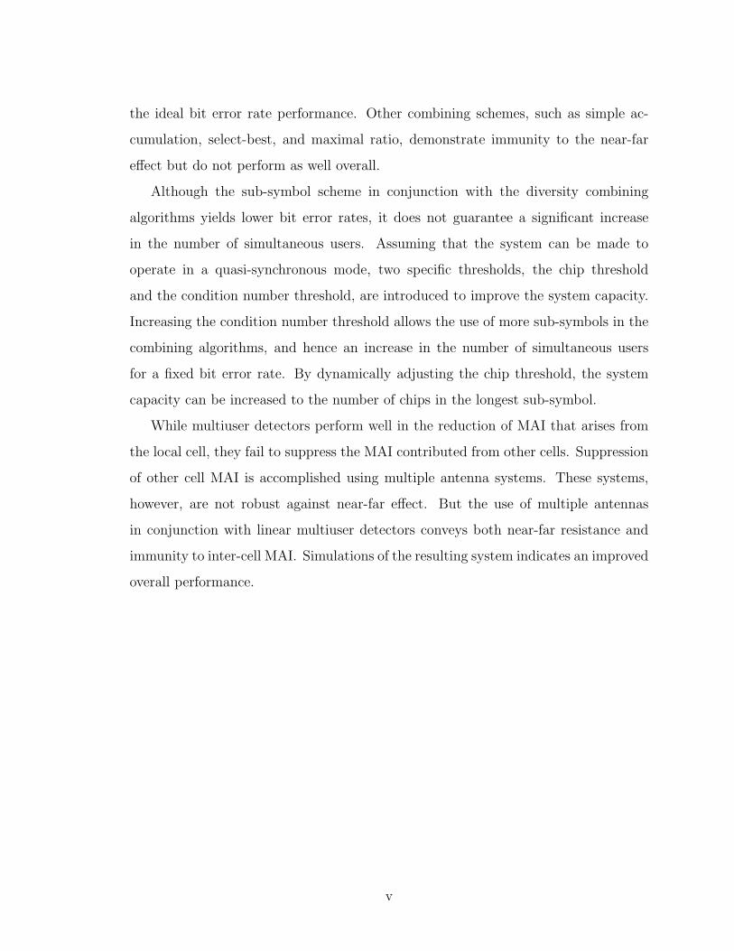
(Last User)
Figure 1.1: Multiuser Detection. Demonstration of a linear multiuser detectorin a DS-CDMA system. Existing systems make decisions on individually demodu-lated signals which contain MAI. Linear multiuser detectors reduce the MAI andallow more users within a given cell.
noise-limited.8 IS-95 systems, by virtue of regarding MAI as additive noise, are clearly
interference-limited.
Multiuser detection is largely the process of mitigating the multiple access inter-
ference (MAI). Several different multiuser detection paradigms have been developed
by previous researchers [36]. In this thesis, we consider linear multiuser detection
schemes as depicted in Fig. 1.1. As this figure illustrates, signals from individual
users, in the uplink, are first demodulated without any knowledge of other users. For
each user, the demodulated signal contains MAI that, in current CDMA systems,
is regarded as added noise. Linear multiuser detection is a standard approach that
involves passing the demodulated signals for all users through a linear filter which
generates cleaner signals for the users with minimal or no MAI. The design of the
linear filter dictates the extent of MAI reduction.
Decoding decisions made on processed signals from multiuser detectors generate
8Interference referred to in this statement corresponds to other-cell interference or unknown MAI.

CHAPTER 1. INTRODUCTION 15
significantly lower bit error rates for individual users. Furthermore, the reduction in
MAI allows more active users within a given cell, thus boosting the capacity of the
system. Thus, multiuser detection brings lower bit error rates and a higher number
of users, both of which account for a capacity increase in a cellular system.
This thesis is concerned with the design of the linear multiuser detector that is
depicted in Fig. 1.1. We consider the design of a system in which a linear multiuser
detector operates on signals from single as well as multiple antennas. Furthermore,
we consider the joint design of the demodulator and the linear multiuser detector.
This approach allows extra flexibility in receiver design and results in significant
performance improvements.
1.4 Contributions
The principal contributions of the research presented in this thesis are:
i) Proposal for a simplified multiuser detector using sub-symbols.
ii) Proposal for diversity combining algorithms for the sub-symbol scheme.
iii) Demonstration by simulation that the bit error rates of condition number based
combining algorithms outperform all other combining algorithms.
iv) Rules for maximizing the number of users in the sub-symbol scheme using proper
thresholds.
v) Discovery that a single sub-symbol is sufficient to outperform the conventional
detector when the sub-symbol scheme is employed for a large number of users
in a quasi-synchronous system.
vi) Demonstration that the performance difference between “zero forcing” and
“minimum mean squared error” multiuser detectors for a synchronous CDMA
system depends on the condition number of the correlation matrices of spreading
sequences.

CHAPTER 1. INTRODUCTION 16
vii) Design for combining linear multiuser detectors with multiple antennas which
outperforms each of these systems considered alone.
Chapters 2–5 and the appendices develop and demonstrate the points above.

Chapter 2
System Model
This chapter introduces the wireless communication model and the direct sequence
code division multiple access (DS-CDMA) transmission environment, and develops
models of different components in a generic DS-CDMA system. The actual mod-
els used for applying specific techniques and algorithms presented in this thesis are
discussed in later chapters.
A mathematical basis for understanding the communications of signals in a wire-
less DS-CDMA communication system is provided in this chapter. The single user
direct sequence spread spectrum communication system is described as a basis for
understanding of multiuser direct sequence spread spectrum communication system.1
Single user end-to-end systems consist of three components: a spread spectrum trans-
mitter, a spread spectrum receiver, and a communication channel through which the
spread spectrum signal propagates. These components of the system are formulated
in Secs. 2.1 and 2.3. A multiuser system is introduced as a superposition of multiple
single user systems in Sec. 2.2 and the uplink in a multiuser system is described in
detail in Sec. 2.5. Section 2.4 describes the spreading sequences for DS-CDMA system
simulations presented in this thesis.
1A multiuser direct sequence spread spectrum system is also known as direct sequence codedivision multiple access or (DS-CDMA) system.
17
CHAPTER 2. SYSTEM MODEL 18
2.1 Single User DS Spread Spectrum System
Spread spectrum (SS) systems are broadly classified as direct sequence (DS) SS sys-
tems and frequency hopped (FH) SS systems. In either case, the generation of a
pseudo noise (PN) signal is required. Most commercial spread spectrum systems use
direct sequence spreading, and these are the systems that are considered in this thesis.
In a SS system, the digital data signal is processed before transmission in such a
way that the processed signal “spreads” over a wider range of frequencies. That is,
the frequency spectrum is widened relative to that with the user signal alone. This
technique has been used by the military for decades and has significant advantages
over non-spread systems: it provides better security, reduces the susceptibility to
jamming, and mitigates interference.2
2.1.1 Spread Spectrum Transmitter
A spread spectrum transmitter generates a spread spectrum signal from a binary
information signal. The binary information signal, represented as a sequence, is
usually obtained from a physical phenomenon. For example, in cellular handsets,
sampling and quantization of a voice signal generates a digital signal that can be
represented as a binary signal [41]. The bit duration of the binary signal depends
upon the source of generation of the binary signal.
Each of the many possible methods [22] of generating a direct sequence spread
spectrum signal requires a pseudo noise sequence or spreading sequence.3 Two meth-
ods of generating the DSSS signal are as follows:
• Mapping the original binary information signal into a binary phase shift keying
(BPSK) signal [42], and then taking the product of the resulting signal and
2The interference mitigated by the use of spread spectrum transmission can either be external,as generated by a jamming device, or it can be internal resulting from the multipath propagation ofthe signal in a wireless environment [22,34,40].
3The terms PN sequence and spreading sequence are used interchangeably. The spreading signaladditionally includes the timing information usually given by the chip duration. “Rate” of thespreading sequence refers to the rate of the corresponding spreading signal.

CHAPTER 2. SYSTEM MODEL 19
Transmitted
Signal
Sinusoidal Carrier
PN Sequence
Rate 1/Tc
PN Sequence
Rate 1/Tb
T c ü T b
Figure 2.1: Spread Spectrum Modulation. A basic direct sequence spreadspectrum transmitter that uses binary phase shift keying (BPSK) modulation.
the spreading signal where the spreading signal is a series of unit amplitude
rectangular pulses each of duration equal to the duration of one chip and of
polarity as determined by the value in the PN sequence.
• XORing the original binary sequence with the spreading sequence preserving
the timing information, and then mapping the resulting sequence into a BPSK
signal.
In practice, channel coding is employed in which the original binary sequence is
replaced by a coded sequence of higher rate. The channel code rate [22] is usually
selected such that the rate of the coded sequence is the same as the rate of the
spreading sequence. Construction of a simple spread spectrum transmitter using
direct sequence spreading is shown in Fig. 2.1. This construction uses the first method
of implementing the spread spectrum transmitter.
Spreading Gain: The spreading gain or the spreading factor, at a spread spec-
trum transmitter, is defined as the ratio of the signal bandwidth after spreading to the
original binary information signal bandwidth. The spreading gain is approximately
equal to the number of chips in one bit duration of the binary information signal [43].

CHAPTER 2. SYSTEM MODEL 20
Received Signal
Sinusoidal Carrier
(Includes Matched Filter)
PN Sequence
Rate 1/Tc
Decision
Device
Figure 2.2: Spread Spectrum Demodulation. A basic direct sequence spreadspectrum receiver that assumes BPSK modulated received signal.
2.1.2 Spread Spectrum Receiver
A direct sequence spread spectrum receiver requires knowledge of the spreading se-
quence used at the transmitter. For a single user spread spectrum system, the only
undesired signal is the additive white gaussian noise, in addition to any interfering
signal.4 When the undesired signal follows the Gaussian distribution, the optimal re-
ceiver for the received signal can be implemented as either a correlator or a matched
filter. The two implementations are functionally equivalent and yield the same out-
put signal. Proakis [22] discusses a somewhat detailed construction of such receiver
implementations. A simplified form of a spread spectrum receiver is shown in Fig. 2.2.
Processing Gain: Processing gain at a spread spectrum demodulator is defined
as the number of chip periods over which the matched filtering or the correlation is
carried out. Usually, the correlation is performed over the bit period or the symbol
period of the binary information signal and processing gain is equal to the number of
chips per bit of the binary information signal. Processing gain signifies the relative
gain of the desired signal compared to the undesired signal [22].
4Historically, a jamming signal, used in military application, is regarded as the interfering signal.In commercial systems, however, the interfering signal is the multiple access interference.

CHAPTER 2. SYSTEM MODEL 21
2.2 Multiuser DS Spread Spectrum System
A single user DS spread spectrum system can be extended to a multiuser system. In
fact, both single user and multiuser spread spectrum systems have similar transmitter
and receiver structures,5 and the multiuser channel is just the superposition of many
single user channels [22].
At the base station, detection of a particular user’s signal assumes that signals
from the other users can be regarded as additive noise. This assumption is based on
the fact that direct sequence spreading results in frequency components with dimin-
ished amplitudes [34], and that the spectrum of a spread spectrum signal resembles
that of additive noise.
Commercial CDMA systems are multiuser DS spread spectrum systems [18]. Since
the multiuser detectors developed in this thesis are designed for DS-CDMA systems,
detailed construction of the transmitter and the receiver for such systems is described
in later sections. Section 2.5 is dedicated to the description of a DS-CDMA transmit-
ter and DS-CDMA channel while later chapters will describe a variety of DS-CDMA
receivers.
2.3 Wireless Communications Model
Wireless cellular communication using DS-CDMA requires understanding not only
the DS-CDMA transmitter and receiver models but also the wireless channel through
which the transmitted signal propagates. In this section, a wireless communication
channel model is developed for performance analysis of various DS-CDMA receivers
described in this thesis.
The channel model is best understood by considering a radio signal propagating
through the channel. It is then used with DS-CDMA transmitter and receiver mod-
els to evaluate the performance of the complete DS-CDMA wireless communication
5In a multiuser system, signal transmitted from a single base station is the sum of signals intendedfor each individual user; the signal received at the base station is the sum of signals individuallytransmitted from users at disparate locations.

CHAPTER 2. SYSTEM MODEL 22
system. The essential parameter of a radio channel is the variation in radio signal
level [11]. The radio signal suffers variations due to many reasons including the mo-
bile user movement, terrain, and building structures [44]. The strength of a received
radio signal is segregated into three main components, each of which is characterized
separately [45, 46]. Thus complete characterization of the radio signal is given by
considering the following three parameters:
i) Path loss resulting from destructive interference of large scale multipath.
ii) Long-term fading distribution considering the attenuation of each path in a
large scale propagation environment.
iii) Short-term fading distribution taking into account the local multipath caused
by objects in the vicinity of transmitter and receiver.
Each of these components of a radio signal model is described in detail in the following
sections:
2.3.1 Path Loss
Path loss is the decrease in radio signal strength as the signal propagates through
space. It is defined as the ratio of transmitted power to received power of a radio
signal. Power in a radio signal decreases as the signal moves away from the transmit-
ter. For a radio signal propagating through free space, the average received power is
given by Friis formula [43,45,47]:
Pr = PtGrGt
(λ
4πd
)2
(2.1)
where Pr is the received power, Pt is the transmitted power, Gr is the gain for receive
antenna, Gt is the gain for transmit antenna, d is the distance from the transmit-
ter, and λ is the wavelength of the transmitted signal. Equation 2.1 describes the
relation between the transmitted and received powers of a radio signal as the radio

CHAPTER 2. SYSTEM MODEL 23
signal propagates through the free space. A decrease in the strength of a signal as it
propagates through free space is called free space loss.
Path loss accounts for free space loss and for interference that may occur due
to large scale reflections from static objects. In a typical urban environment, the
propagation of a radio signal is accomplished via direct path, reflection, scattering
and diffraction [44]. Thus the propagating signal suffers not only from variations in
amplitude and phase but also from a spread in the received signal. The temporal
spread in received signal relative to the transmitted signal is called delay spread,
and the inverse delay spread is called coherence bandwidth [43, 46]. For narrowband
channels,6 the received signal can be regarded as multiple copies of the transmitted
signal, received one after the other, and typically decreasing in amplitude [11,46].
Of the models used to characterize the path loss in a radio channel, the 2-ray and
the 10-ray models are the most popular [43,48]. These models take into account the
free space loss and the interference that occurs as a result of large scale reflection. Ray
tracing techniques are used as a design tool for such models [49–51]. Although ray
tracing models are only approximate, yet they are complex to develop. Analysis of
ray tracing models results in power fall-off rates that are generally higher than those
given by free space path loss [43, 52]. Simplification of ray tracing models results in
received power that can be expressed as a function of distance from the transmitter.
A simplified model can be expressed in the following equation:
Pr = Pr0
[d0
d
]n
(2.2)
where Pr0 is the power received at a distance d0 from the transmitter, and n is the
propagation index typically ranging from 2 to 5 [53]. The above model is valid for
distances d > d0, where d0 is the reference distance for the antenna far-field. The
distance d0 is usually determined by propagation measurements [52].
The propagation index depends on the environment as well as the distance from
6A channel is regarded as narrowband if the coherence bandwidth is greater than the signalbandwidth; otherwise, the channel is regarded as wideband.

CHAPTER 2. SYSTEM MODEL 24
the transmitter. Thus, there are models (see [53] and the references therein) that
specify a value of propagation index based on the distance from the transmitter. For
distances less than d0, the propagation index is usually taken as 2, corresponding
to free space, while for distances greater than d0, the propagation index usually
lies between 2 and 5 as dictated by the propagation measurements. References [52]
and [54] report propagation measurements at 800 MHz, for example. In summary,
these measurements indicate that path loss falls off approximately as d2 up to a critical
distance d0 and sharply increases with distance beyond the critical distance.
2.3.2 Lognormal Fading
The path loss described in Sec. 2.3.1 is the result of free space loss plus the destruc-
tive combination of different replicas of the transmitted signal. Each replica of the
transmitted signal also fades individually as it passes through various obstacles and
structures [45,46]. Thus, the received signal, given by the combination of such repli-
cas, exhibits fluctuations in the amplitude in addition to the path loss. The random
fluctuation in the received signal due to large scale objects is termed long-term fading
or shadowing, and has been characterized as following a lognormal distribution [45].
Shadowing is the fluctuation in the received signal superimposed over the path
loss. Therefore, shadowing distribution has a mean that is equal to the path loss.
The standard deviation of the lognormal shadowing distribution typically ranges from
5–12 dB [11]. Thus the received signal power exhibits a 5–12 dB variation around a
signal power that would be expected if only path loss were taken into account.
Lognormal shadowing is completely characterized by the mean and standard de-
viation of the distribution [55] which are usually obtained through empirical data
[56,57]. The autocorrelation of the lognormal shadowing depends upon the surround-
ing building sizes. Measurement data, reported by Gudmundson in [58], address the
autocorrelation properties of the lognormal shadowing.

CHAPTER 2. SYSTEM MODEL 25
2.3.3 Short-Term Fading
Variation in signal due to local multipath is referred to as short-term fading. Local
multipath or short-range multipath, a result of presence of objects in close vicinity to
the transmitter and the receiver, imparts additional statistical characteristics to the
radio signal. Short-term fading has a distribution whose local mean is given by the
lognormal distribution. Of the several short-term statistical fading models that have
been developed in the literature [44,46,59], the most widely accepted is developed in
the following and used for simulations in later chapters.
Complete characterization of the channel consists of considering a few dominant
large-scale multiple paths, where each of these paths is comprised of short-range
multipath component waves, and is characterized independently [11]. To derive the
expression for one dominant path, let x(t) be the transmitted signal given by:
x(t) = �{s(t)ej(2πfct+φ0)
}(2.3)
where s(t) is the complex baseband signal, fc is the carrier frequency, and φ0 is an ar-
bitrary initial phase that can be considered as zero for further analysis. Now, consider
a particular large-scale path consisting of N0 short-range multipath components. The
short-range multipath components are generated by reflection and scattering from lo-
cal scatterers. The received signal can, therefore, be expressed as:
r(t) = �{ N0∑
n=1
αn(t)s(t − τn(t))ej2π(fc+∆fn(t))(t−τn(t))
}(2.4)
where N0 is the total number of multipaths, τn is the delay of the n-th multipath
component, and ∆fn designates the doppler shift of that component. Path loss,
lognormal shadowing, and antenna gain are factored into αn, which designates the
net amplitude gain for the large-scale path given by Eq. 2.4. Defining the parameter
φn(t) = (fc+∆fn(t))τn(t)−t∆fn(t) which indicates the phase imparted by the channel

CHAPTER 2. SYSTEM MODEL 26
to the n-th multipath component, the above expression can also be written as:
r(t) = �{[ N0∑
n=1
αn(t)e−jφn(t)s(t − τn(t))]ej2πfct
}(2.5)
We define the multipath delay spread as the maximum difference in arrival times
of any two multipath components. The relative values of the signal bandwidth and
inverse delay spread classify the channel as a narrowband or wideband. Modelling of
narrowband channels is relatively simple because relative delays for individual multi-
path components are assumed to be negligible [11,43], and s(t−τn(t)) is approximated
by s(t) [46]. Therefore, for a narrowband channel, a received path can be written as:
r(t) = �{
s(t)ej2πfct( N0∑
n=1
αn(t)e−jφn(t))}
(2.6)
which contains an additional complex scaling factor in parentheses as compared to
the original signal. To characterize the scale factor, let7 s(t) = 1, which results in:
r(t) = �{( N0∑
n=1
αn(t)e−jφn(t))ej2πfct
}(2.7)
r(t) = rI(t) cos 2πfct + rQ(t) sin 2πfct (2.8)
where rI(t) is the in-phase and rQ(t) is the quadrature component of r(t). The
components of r(t) are given by:
rI(t) =
N0∑n=0
αn(t) cos φn(t) (2.9)
rQ(t) =
N0∑n=0
αn(t) sin φn(t) (2.10)
It should be noted that the number of short-range local multipath components, N0,
7As seen from Eq. 2.3, taking s(t) = 1 yields a single tone, and hence renders the transmittedsignal narrowband. This is necessary for proper characterization of the scale factor.

CHAPTER 2. SYSTEM MODEL 27
also depends on position, and hence on time for a user in motion. The value of N0 is
generally very large for typical environments, such that the central limit theorem is ap-
plicable [55], rendering the in-phase and quadrature components as Gaussian random
processes. The envelope of each path of the received signal |r(t)| =√
r2I (t) + r2
Q(t),
therefore, follows a Rayleigh distribution8 assuming no line-of-sight path exists. If
a line-of-sight path is present, then the in-phase and quadrature components of the
received signal are not zero-mean [60, 61]. In such a case, the signal envelope has a
Rician distribution [46,61].
2.4 Spreading Sequences
All spread spectrum systems use one or more spreading codes9 to achieve spreading
of the desired signal prior to transmission. Selection of spreading codes for a typ-
ical application depends on the application itself and on the specific properties of
the spreading codes. For single user communications in a multipath environment the
most important factor is to achieve the ability to resolve the multipath. To do this
effectively, the spreading codes must have excellent autocorrelation properties, ideally
a delta function. Similarly, for a multiuser system in a non-multipath environment
the most important factor in selecting the spreading sequences is the ability to min-
imize the multiaccess interference. The multiaccess problem can be addressed if the
spreading sequences are selected such that the maximum value of cross-correlation is
minimized [22,36].
Commercial CDMA systems are multiuser systems in multipath environment.
Therefore, the spreading sequences for CDMA systems are selected by considering
both their autocorrelation and cross-correlation properties. Furthermore, CDMA sys-
tems are cellular and require separation of intra-cell as well as inter-cell users. This
requires two levels of spreading achieved by a combination of two spreading codes,
8This also implies that the received power in this signal path follows an exponential distribution.9Spreading codes are generated from pseudo random or pseudo noise (PN) sequences. This is
because PN sequences exhibit such statistical properties that are desired of spreading codes.

CHAPTER 2. SYSTEM MODEL 28
referred to as channelization codes and scrambling codes. Multiple spreading is de-
scribed in detail elsewhere [35]. Subsequent sections discuss the spreading sequences
commonly used in commercial DS-CDMA systems and in our simulations as well.
2.4.1 Maximal Length Sequences
Maximal length sequences or m-sequences are the most widely recognized and used
pseudo noise (PN) sequences; they can be generated by two methods by using a linear
feedback shift register (LFSR). The first using simple LFSR and the other using
modular LFSR. Each of the LFSR, either simple or modular, can be represented by
means of a polynomial [22].
A sequence, generated by an LFSR with m registers, is said to be a maximal
length sequence or an m-sequence if its length is L = 2m − 1. An m-sequence is
generated when the LFSR structure represents a primitive polynomial [32, 62]. The
length of the m-sequence is the possible number of states an LFSR can take,10 except
for an all zero state. For an LFSR, an m-sequence of length L provides the best
autocorrelation properties [22,32], as follows:
R(n) =
L n = 0, L, 2L, · · ·
−1 otherwise
(2.11)
An example generation of an m-sequence using a simple LFSR is shown in Fig. 2.3.
The same m-sequence can also be generated by a modular LFSR as shown in Fig. 2.4.
The constructions in Fig. 2.3 and Fig. 2.4 are equivalent: they generate the same
m-sequence, represent the same polynomial 1 + x2 + x5, and implement the same
difference equation x[i] = x[i − 2] ⊕ x[i − 5].
Another representation of both constructions is written as [2 5]S ≡ [3 5]M . It
should be noted that [ ]S notation indicates the quotients of the primitive polynomial
10Each register in an LFSR is a binary register and has two possible states. The state of an LFSRwith r binary registers is an r-tuple where each element indicates the state of one distinct binaryregister.

CHAPTER 2. SYSTEM MODEL 29
1 5432
Figure 2.3: Simple LFSR. Simple linear feedback shift register realization of apolynomial given by the difference equation x[i] = x[i − 2] ⊕ x[i − 5].
1 5432
Figure 2.4: Modular LFSR. Modular linear feedback shift register realizationof a polynomial given by the difference equation x[i] = x[i − 2] ⊕ x[i − 5].
representing the LFSR, while the [ ]M notation indicates the quotients of a primitive
polynomial that is the reciprocal of the primitive polynomial representing the LFSR.11
The construction used by Sarwate in [32] is similar to the simple LFSR but the
representing polynomial is the reciprocal of the one representing the construction
of simple LFSR in Fig. 2.3. The ETSI proposal for WCDMA standard [63] uses the
notation of Sarwate [32]. Therefore, for our simulations, we implement the reciprocals
of the polynomials given in proposed standards [63] using the structures of Fig. 2.3
and Fig. 2.4.
2.4.2 Gold Sequences
The m-sequences have excellent autocorrelation properties but their cross-correlation
properties do not follow any particular rules [40,64] and typically exhibit undesirably
high values [22]. Furthermore, the number of m-sequences for a given number of
registers in an LFSR is limited. Gold sequences address these problems, and are
11The reciprocal of a polynomial is obtained by reversing the quotients; if p(x) is a polynomialof degree n, its reciprocal is given by xnP (1/x). The reciprocal of a primitive polynomial is alsoprimitive [32,40].

CHAPTER 2. SYSTEM MODEL 30
derived by combining the m-sequences from two LFSRs [65, 66].12 In comparison
to m-sequences, Gold sequences provide larger sets of sequences and exhibit better
cross-correlation properties [22,40].
Gold sequences are generated from two equal length m-sequences that form a so-
called preferred pair. The cross-correlation of two m-sequences that form a preferred
pair is tri-valued [67] and it takes the values from the set {−1,−t(m), t(m) − 2},where t(m) = 1 + 2�(m+2)/2�, and m is the number of binary shift registers in the
LFSR. A requirement for the generation of Gold sequences is that m should be equal
to 2 Modulo 4. Under this condition, GCD (t(m), 2m−1) = 1, i.e t(m) and 2m−1 are
relatively prime [32]. Thus, if u is an m-sequence, a t(m)-decimated version of u,
denoted by v = u [t(m)] is also an m-sequence, and u and v form a preferred pair [32].
A set of 2m + 1 Gold sequences can be generated from u and v as given by the set
{u, v, u ⊕ T i{v}}, where T i{v} indicates the right (or left) shift of sequence v by i
bits, and i varies from 0 to L − 1, where L is the length of sequences that form the
preferred pair.
2.4.3 Kasami Sequences
Kasami sequences also address the two undesirable properties of the m-sequences:
smaller sets of sequences and potentially higher cross-correlation values. Kasami
sequences can be generated either as a small set or as a large set. The small set
has better cross-correlation properties, while the large set provides more sequences to
choose from. Generation of Kasami sequences involves a method similar to the one
used to generate the Gold sequences, as given below.
2.4.3.1 Small Set
To generate the small set Kasami sequences, an m-sequence, denoted as u, is first
generated. Let the length of the sequence u be L, and m be the number of binary
registers in the LFSR, such that L = 2m − 1. One period of the sequence u is
12Combining two m-sequences refers to performing Modulo 2 addition of the two sequences.

CHAPTER 2. SYSTEM MODEL 31
decimated by 2m/2 + 1 to generate a sequence w of length{2m − 1
}/{2m/2 + 1
}; the
length of w simplifies to 2m/2 − 1. Next, 2m/2 + 1 repetitions of w are concatenated
to form a sequence v of length L. The small set Kasami sequences are then given by
the set {u, u ⊕ T i{v}}, where T i{v} indicates the right (or left) shift of sequence v
by i bits, and i varies from 0 to 2m/2 − 1.
2.4.3.2 Large Set
The large set Kasami sequences are generated either from the Gold set or from the
Gold-like set.13 Large set Kasami sequences includes the Gold set and the small
set Kasami sequences as the subsets. The procedure to generate large set Kasami
sequences can be found in the literature, e.g., [32] and is not discussed here.
2.5 CDMA Uplink Signal Model
A baseband model of a CDMA uplink is shown in Fig. 2.5. The signal received at the
base station is the summation of signals from all users, multipath components for each
user’s signal, and additive white gaussian noise (AWGN). Figure 2.5 also includes
channel encoders for each transmitter. For simulations performed without channel
encoding, the encoder has no effect. For simulations that use channel encoding a
convolutional encoder of constraint length 5 is used [22].
There are Nu users in the system and the data signals from these users are des-
ignated as d1(t), d2(t), . . . , dNu(t). The data symbols within the data signals are
spread by multiplying with respective spreading sequences K1(t), K2(t), . . . , KNu(t).
The channel introduces delays τ1, τ2, . . . , τNu to signals from different users, and
A1(t), A2(t), . . . , ANu(t) are the fading coefficients for the single resolvable path of
each user.14 The spreading sequences are the periodic extensions of single periods
13Large set Kasami sequences can be generated for all even values of m, the number of binaryregisters in LFSR. When m is equal to 2 Modulo 4, large set Kasami sequences are generated byfirst generating Gold sequences. When m is equal to 0 Modulo 4, it is not possible to generate Goldset and large set Kasami sequences are generated by first generating Gold-like sequences [32].
14The product with fading coefficients in Fig. 2.5 is equivalent to a time varying convolution with
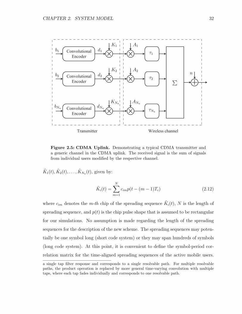
CHAPTER 2. SYSTEM MODEL 32
Convolutional
Encoder
Convolutional
Encoder
Convolutional
Encoder
Transmitter Wireless channel
b1
b2
bNu
d1
d2
dNu
K1
K2
KNu
A1
A2
ANu
τ1
τ2
τNu
∑ n
Figure 2.5: CDMA Uplink. Demonstrating a typical CDMA transmitter anda generic channel in the CDMA uplink. The received signal is the sum of signalsfrom individual users modified by the respective channel.
K1(t), K2(t), . . . , KNu(t), given by:
Ki(t) =N∑
m=1
cimp(t − (m − 1)Tc) (2.12)
where cim denotes the m-th chip of the spreading sequence Ki(t), N is the length of
spreading sequence, and p(t) is the chip pulse shape that is assumed to be rectangular
for our simulations. No assumption is made regarding the length of the spreading
sequences for the description of the new scheme. The spreading sequences may poten-
tially be one symbol long (short code system) or they may span hundreds of symbols
(long code system). At this point, it is convenient to define the symbol-period cor-
relation matrix for the time-aligned spreading sequences of the active mobile users.
a single tap filter response and corresponds to a single resolvable path. For multiple resolvablepaths, the product operation is replaced by more general time-varying convolution with multipletaps, where each tap fades individually and corresponds to one resolvable path.

CHAPTER 2. SYSTEM MODEL 33
Therefore,
Rij(t) =
∫symbolperiod
Ki(t)Kj(t) (2.13)
is the element of symbol-period correlation matrix in the i-th row and j-th column.
The signal at the receiver front end is the sum of signals transmitted by individual
mobile users, modified by the channel gain for each user and contaminated by additive
white gaussian noise, as depicted in Fig. 2.5. Therefore, the received signal r(t) can
be written as:
r(t) =Nu∑j=1
(Kj(t − τj)Aj(t − τj)dj(t − τj)
)+ n(t) (2.14)
where n(t) is additive white gaussian noise (AWGN) with variance σ2n. The received
signal in the above expression is the one present at the front end of any CDMA system
receiver. The signal at the output of the receiver depends upon the receiver structure.
Various receiver types, conventional and more advanced, are discussed in subsequent
chapters.

Chapter 3
Linear Synchronous Receivers
This chapter introduces some of the receivers1 employed for the DS-CDMA systems.
The received signal model used in these receivers is as derived in Chapter 2. A single
user matched filter receiver, described in Sec. 3.1, is the simplest of all DS-CDMA
receivers. ‘Zero forcing’ and ‘minimum mean squared error’ detectors are described
in Sec. 3.2. The remainder of this chapter is dedicated to the algorithms used in more
advanced linear multiuser detectors.
3.1 Single User Matched Filter
The basic CDMA receiver, popularly known as a conventional detector [37], employs
a single user matched filter (SUMF) which is often implemented as a correlator. In
SUMF detection, the signal from each user is demodulated individually without any
knowledge of signals from other users. There is one SUMF detector at the base station
for each active user, and the output of each detector is determined independently of
the output of any other detector. The description, construction, and performance of
the SUMF detector are explained in what follows.
The SUMF detector is a maximum-likelihood detector in the sense of maximizing
the signal-to-noise ratio (SNR) for a particular user without regard to the signals
from other users. Thus, it is the optimal detector (see [22] and [68] for details) if
1The terms receiver and detector are used interchangeably.
34

CHAPTER 3. LINEAR SYNCHRONOUS RECEIVERS 35
the despread and demodulated signal for each user contains only additive white noise
(AWN). This detector also minimizes the probability of error for the single user in
case of additive white gaussian noise (AWGN) [36]. The assumption that signals from
other users sharing the channel can be neglected is valid only when the spreading
sequences of all the users are orthogonal2 to each other and remain so when the
signal is received at the base station after passing through the wireless propagation
environment. However, non-zero cross-correlations among spreading sequences lead
to multiple access interference (MAI) which, in general, increases with the number of
users [36]. Even if the spreading sequences are chosen to be orthogonal to each other
to start with, the orthogonality is lost when the signals pass through the multipath
environment and arrive at the base station with random delays [33,46].
This section details the construction of the single user matched filter. For this
purpose, we utilize the channel and received signal model as described in Chapter 2.
Because a signal received at the front end of any CDMA receiver depends in part
upon the channel through which the received signal has propagated, we first describe
synchronous and asynchronous classes of DS-CDMA channels. Next, we describe the
SUMF receivers for these two DS-CDMA channel classes.
3.1.1 CDMA Channel Classification
CDMA systems are classified as either synchronous or asynchronous on the basis
of the timing method for signals received from different users. In the synchronous
channel, the basic assumption is that the users’ transmission times are controlled in
a way that the signals received from different users coincide at the bit boundaries
observed at the base station receiver.3 Since the users are geographically separated
2Orthogonality of two spreading sequences in the received signal means that the portion of thesignal from one user results in zero output from the receiver of the other user. That is, the receiverfor first user will have zero output, except for the AWGN, if the signal transmitted from the firstuser is cut off, irrespective of the signal from the second user.
3Strictly speaking, in a synchronous CDMA system, signals received from different users coincidein time at the chip boundaries as well as the bit boundaries. Asynchronous systems do not posesuch requirement. Simulation results presented in this thesis use one sample per chip, therefore, therequirement of chip alignment is implicit for synchronous and asynchronous CDMA systems.

CHAPTER 3. LINEAR SYNCHRONOUS RECEIVERS 36
One Symbol (N chips)
P chips N-P chips
Figure 3.1: QS-CDMA Symbol. Depicting a typical symbol in a QS-CDMAsystem. The spreading gain of the system is N and symbol boundaries from varioususers are allowed to fall within the first P chips of the symbol.
from one another and often are in motion, a synchronous system requires timing
control for each and every user.
An asynchronous system does not require the received symbols from different users
to be time aligned at symbol boundaries at the base station. It is a more general
CDMA system, and most commercial systems fall in this category. Specifically, the
reverse links in commercial CDMA systems are asynchronous due to a lack of accurate
control on user transmission instants.
An asynchronous CDMA system with approximately aligned symbols is sometimes
referred to as a quasi-synchronous code division multiple access (QS-CDMA) system.
In QS-CDMA, the uncertainty in symbol alignment lies within a small fraction of the
total number of chips in the spreading sequence. For example, as shown in Fig. 3.1,
if N is the total number of chips in one symbol and P is the smallest number such
that any symbol start time at the receiver does not fall within N − P chips, then
the uncertainty in symbol alignment for such a system is P chips. The signal in
the period of uncertainty may be blanked out by appending blank chips to the actual
spreading sequence [69], thereby increasing the symbol time.4 For our example, where
P is the period of uncertainty and N is the number of chips per original symbol, the
symbol period is extended to N +P chips per symbol. There are QS-CDMA systems,
however, in which the period of uncertainty in alignment is not blanked out. In this
case, the system is exactly the same as an asynchronous system with a smaller degree
of asynchronism [70].
4The period of uncertainty is blanked out by a decrease in symbol rate rather than an increasein chip rate because actual dependence of uncertainty is on time and not the number of chips.

CHAPTER 3. LINEAR SYNCHRONOUS RECEIVERS 37
Received
Signal
K1
K2
KNu
∫symbolperiod
∫symbolperiod
∫symbolperiod
y1
y2
yNu
d1
d2
dNu
Figure 3.2: SUMF Receiver. A typical CDMA uplink model with single usermatched filter for Nu distinct users; time-dependence of the parameters have beenomitted for simplicity. For synchronous case, the delays τ are made the same.
3.1.2 SUMF for Synchronous CDMA Systems
Currently deployed DS-CDMA receivers use SUMF detection. The detection is per-
formed by correlating a locally generated replica of the spreading sequence of the
user of interest with the incoming signal, as shown in Fig. 3.2. The correlation is
performed over a symbol period and it is assumed that the symbol-long portion of
the locally generated spreading sequence correlates weakly with spreading sequences
of the other users. For a particular symbol, the output of the SUMF is given by:
yi(t) =
∫symbolperiod
r(t)Ki(t − τj) (3.1)
where r(t) is given by Eq. 2.14 and τj is the channel delay for the j-th user. For a
synchronous system, Eq. 3.1 reduces to
yi(t) =Nu∑j=1
(Rij(t)Aj(t)dj(t)
)+ ni(t) (3.2)
CHAPTER 3. LINEAR SYNCHRONOUS RECEIVERS 38
where ni(t) is the noise n(t) in Eq. 2.14 processed by the i-th matched filter. That is,
ni(t) is the gaussian noise with variance Rii(t)σ2n. Equation 3.2 can also be written
as:
yi(t) = Rii(t)Ai(t)di(t) +Nu∑j=1j �=i
(Rij(t)Aj(t)dj(t)
)+ ni(t) (3.3)
It can be seen from the above expression that yi(t) has three components: the desired
signal Rii(t)Ai(t)di(t), the additive gaussian noise ni(t), and the remainder terms
that arise as a result of non-zero cross correlation between spreading sequences. The
undesired terms in yi(t) comprise the additive noise and the multiple access interfer-
ence (MAI) which are neglected by the SUMF detector that performs the slicing or
decision operation on yi(t).5
MAI degrades the system performance and limits the capacity of CDMA systems
[71]. It depends on other users’ signals, as demonstrated by Eq. 3.3, and does not
change with signal-to-noise ratio (SNR). This leads to a BER floor that is always
exhibited by the SUMF detector regardless of whether the system is synchronous or
asynchronous.
3.1.2.1 Orthogonal Sequences
When the DS-CDMA system can be guaranteed to be synchronous,6 it is preferable
to use orthogonal sequences for spreading. This results in the complete elimination of
MAI, so that the SUMF detector actually achieves the AWGN performance.7 From
Eq. 3.2 the demodulated signal8 for the i-th user can, therefore, be written as:
yi(t) = Rii(t)Ai(t)di(t) + ni(t) (3.4)
5Slicing or decision operation for digital signals produces the data from the transmitted alphabet.For equiprobable binary signals transmitted as +1 and -1, slicing operation at the output of a receiverproduces +1 when the receiver output is greater than 0 [22].
6Accurate control over transmission instants of all the users is required to guarantee that thesystem will be synchronous.
7Orthogonal sequences in a synchronous system will eliminate the local cell MAI. Interferencefrom other cells may still cause the performance to be deteriorated.
8Signal that appears at the output of SUMF is regarded as the demodulated signal.

CHAPTER 3. LINEAR SYNCHRONOUS RECEIVERS 39
which is obtained by setting all the cross-correlation terms, Rij(t), i �= j, equal to zero.
When the additive noise is gaussian, the error probability in detecting yi(t) is given by
the tail of the gaussian distribution [68] and can be derived as Q(√
SNR) [22], where
SNR is the ratio of the signal power to the noise power, and the Q-function is the tail
of the ‘standard’ gaussian probability distribution.9 Thus, the error probability, Pe,1
in the detection of yi(t) is given by:
Pe,1 = Q
(√Rii(t)Ai(t)
σ
)(3.5)
which is the same as that for a single user in AWGN channel [22].
3.1.2.2 Semi-orthogonal sequences
Semi-orthogonal sequences do not exhibit zero cross-correlation, but their cross-
correlation properties are generally better than those of orthogonal sequences [22,33].
When the transmission instants of individual users can not be controlled accurately,
symbols from users will be received asynchronously at the base station. In such a
case, spreading sequences generally are chosen such that the cross-correlation and
hence the MAI is minimized. The Gold and Kasami sequences discussed in Sec. 2.4
are examples of sequences that exhibit good cross-correlation properties [22]. For
example, Kasami sequences exhibit a tri-valued cross-correlation function [32]. Semi-
orthogonal sequences limit the MAI in an asynchronous system at the expense of
producing some MAI when the system happens to be synchronous.
MAI under synchronous operation can be directly computed from Eq. 3.2. To
perform a quantitative analysis of MAI, consider a system with two users, so that the
9A standard gaussian probability distribution is defined as having zero mean and unit variance[55]. Q-function is defined as Q(x) = 1√
2π
∫ x
−∞ e−u2/2du and is related to the complementary errorfunction as Q(x) = 1
2erfc( x√2).

CHAPTER 3. LINEAR SYNCHRONOUS RECEIVERS 40
SUMF outputs from Eq. 3.2 can be written as:
y1(t) = R11(t)A1(t)d1(t) + R12(t)A2(t)d2(t) + n1(t) (3.6)
y2(t) = R21(t)A1(t)d1(t) + R22(t)A2(t)d2(t) + n2(t) (3.7)
Equation 2.13 dictates that R11(t) = R22(t) and R12(t) = R21(t). Thus, by symmetry,
the probability of error in the detection of y1(t) is the same as the probability of error
in the detection of y2(t). Conditioning on the symbol of the second user, this error
probability Pe,2 can be derived from the above equations and is given by [36]:
Pe,2 =1
2Q
(R11A1 − R12A2√
R11σ
)+
1
2Q
(R11A1 + R12A2√
R11σ
)(3.8)
where the time dependence of variables has been removed for the sake of simplicity.
The equation above assumes that the data symbol from the interfering users takes
on each of the possible binary values with 50% probability. Since the Q-function is
monotonic, it can be seen that Pe,2 is greater than Pe,1 and reduces to Pe,1 when the
cross-correlation R12 is set to zero: probability of error in detection for a two-user
system is greater than the corresponding probability for a single user system. The
analysis can be extended to an arbitrary number of users in a similar fashion (see
Chapter 3 of [36] for details). In summary, for the synchronous DS-CDMA channel,
the error probability depends on the following parameters:
i) Relative magnitudes of the received signals.
ii) Cross-correlation values of the spreading sequences.
iii) Power of the additive noise.
3.1.3 SUMF for Asynchronous CDMA Systems
Asynchronous systems, in which received symbols from different users are not time-
aligned, respond to the SUMF in the same way as do synchronous systems [36]. In

CHAPTER 3. LINEAR SYNCHRONOUS RECEIVERS 41
d11 d12 d13
d21 d22 d23
Figure 3.3: Interfering Symbols. Depicting the MAI for the case of two asyn-chronous users. Each symbol from a user is contaminated by two different symbolsfrom the other user.
an asynchronous system, one symbol of each user is “contaminated” by at most two
symbols from each of the other users. Thus, in a K-user system, where there are
(K − 1) interfering users, the are (K − 1) interfering symbols in the synchronous case
and up to 2(K − 1) interfering symbols in the asynchronous case. Figure 3.3 depicts
the interfering symbols in an asynchronous system with two users. An increase in the
number of interfering symbols from (K − 1) to 2(K − 1) does not imply an increase
in MAI in an asynchronous system compared with the synchronous system, because
the cross-correlation products are computed only over the overlapping portion of the
symbols. In this case, the MAI and the bit error probability are dependent upon the
following parameters:
i) Relative magnitudes of the received signals.
ii) Partial cross-correlation values of the spreading sequences.
iii) Power of the additive noise.
Partial cross-correlation values among the spreading sequences are dependent upon
how much one symbol overlaps with the other symbol, which in turn depends upon
the transmission instants of the individual users and their distances from the base
station. It may be probable that the partial cross-correlation values between two
sequences exceed the full-period cross-correlation.
When data signals and spreading sequences are purely random, the signal value
within each chip interval from each user is completely random. In this instance,

CHAPTER 3. LINEAR SYNCHRONOUS RECEIVERS 42
interfering portions of two symbols from each interfering user can be thought of as just
one symbol. For example, in Fig. 3.3, portions of d21 and d22 that interfere with d12 can
be regarded as a single interfering symbol. Thus, with random spreading sequences,
the asynchronous and the synchronous systems will exhibit the same average bit error
rate.
3.1.4 SUMF in Rayleigh Fading Environment
The error probabilities discussed in the above sections assume that the received signal
amplitudes Ai(t) are deterministic. In a fading environment, however, these coeffi-
cients are random and we need to average the error probabilities over the fading
distribution [36,43]. In widely accepted models, as discussed in Sec. 2.3.3, the fading
coefficients usually follow the Rayleigh distribution. Averaging the error probabilities
according to a Rayleigh distribution results in much higher bit error rates [36,71], as
compared with those obtained in the case of deterministic amplitudes. For a single
user, the error probability in Rayleigh fading environment falls linearly with SNR,
whereas in AWGN, the error probability falls exponentially with SNR [22,72,73]. Sim-
ulation results for bit error rates with SUMF in Rayleigh faded channels are shown
in Sec. 3.2, where a comparison with linear multiuser detectors is made.
3.1.5 SUMF for Resolvable Multipath: RAKE Receiver
A RAKE receiver combines independently fading paths in a DS-CDMA receiver.
Thus a RAKE receiver implements multipath diversity combining. It consists of a
number of SUMF receivers, each of which detects one fading path. The resulting
paths are then combined using one of the three algorithms for diversity combining:
Selection, Equal-gain, and Maximal Ratio. A thorough analysis of selection diversity
combining algorithms is given in [74] and maximal ratio combining is discussed in [75].
A textbook treatment of diversity combining algorithms is provided in [43].
DS-CDMA systems are well-suited for diversity reception because spreading ren-
ders the channel wideband, thereby making it easier to resolve multiple path at the

CHAPTER 3. LINEAR SYNCHRONOUS RECEIVERS 43
Received
Signal Linear
Filter
K1
K2
KNu
∫symbolperiod
∫symbolperiod
∫symbolperiod
y1
y2
yNu
y1
y2
yNu
d1
d2
dNu
Figure 3.4: Linear Multiuser Detector. A generic linear multiuser detectorconsists of a linear filter applied at the outputs of a set of single user matchedfilters. The objective is to reduce the MAI that appears at the output of singleuser matched filters.
receiver [46]. In fact, multipath resolution and combining is one of the major benefits
of DS-CDMA system over other multiaccess wireless communication systems. Diver-
sity combining is a powerful technique to mitigate the effects of fading, the idea being
that if the signal along one path fades, other independent fading paths are less likely
to experience fading at the same time.
3.2 Receivers with Linear Multiuser Detection
This section describes the analysis and simulation results of linear multiuser receivers
employing a single receive antenna; linear multiuser detectors with multiple antennas
will be discussed in chapter 5.
Figure 3.4 depicts a generic linear MUD receiver. A comparison of linear MUD
with SUMF of Fig. 3.2 indicates that signals from SUMFs are passed through a linear
filter before performing the slicing or decision operation. The design of linear filter
depends on the specific signal processing algorithm implemented by the detector.
Linear MUDs can be based on either the zero forcing (ZF) criterion or the minimum

CHAPTER 3. LINEAR SYNCHRONOUS RECEIVERS 44
mean squared error (MMSE) criterion. Both of these designs are discussed in the
following sections.
3.2.1 Zero Forcing Linear Multiuser Detector
A ZF linear MUD, or simply ZF MUD, attempts to completely eliminate the MAI
in a DS-CDMA system without regard to AWGN. For the purpose of this section,
we consider a synchronous CDMA system. The ZF linear MUD for an asynchronous
system is considered in Sec. 3.3.
Using Eq. 3.2 for all the users, we write the received signal after despreading in
matrix form :
�y = RA�d + �n (3.9)
where R is the Kasami10 correlation matrix whose elements are defined by Eq. 2.13,
A is a diagonal matrix that contains Rayleigh fading coefficients for each user, and
�d is the vector of transmitted symbols, which may or may not be coded.11 Since R
is not a diagonal matrix in general, it reflects the MAI introduced due to non-zero
cross-correlations. For a synchronous system that uses orthogonal sequences R is a
diagonal matrix indicating that no MAI exists in the system.
For the derivation of zero forcing (ZF) linear multiuser detector filter, we set
the additive gaussian noise term to be equal to zero in Eq. 3.9. Then, by setting the
required response to be equal to A�d, the ZF linear filter is given by R−1. To eliminate
MAI, ZF MUD performs the R−1 operation on the received signal �y [37], as depicted
in Fig. 3.5. Thus the vector signal, �ydecor, at the output of ZF linear MUD can be
written as:
�ydecor = R−1�y = A�d + R−1�n (3.10)
10In general, R is the cross-correlation matrix of the spreading sequences. Since we use Kasamisequences for the simulation results reported in this thesis, we specialize R to denote Kasami corre-lation matrix.
11Communication systems generally employ channel encoding prior to transmission; this involvesgenerating a coded bit sequence from the uncoded bit sequence [22]. We consider �d as a genericdata vector: it contains coded symbols if any encoding is used on the channel, otherwise �d simplycontains the raw data.

CHAPTER 3. LINEAR SYNCHRONOUS RECEIVERS 45
Received
Signal
K1
K2
KNu
∫symbolperiod
∫symbolperiod
∫symbolperiod
y1
y2
yNu
y1
y2
yNu
d1
d2
dNu
R−1
Figure 3.5: ZF Linear MUD. Depicting the zero forcing linear multiuser detec-tor filter applied at the outputs of a set of single user matched filters. The resultingsignal contains no MAI if the CDMA system is synchronous.
Decisions made on signs of �ydecor, at the output of ZF MUD, are always correct if
additive noise term is neglected. However, for low SNRs, the R−1�n term becomes
significant, resulting in poor performance. The BER performance of a ZF MUD is
compared with a single user matched filter detector in Fig. 3.6. Simulation results
shown in Fig. 3.6 are obtained using parameters specified in the WCDMA standard
proposal submitted by ETSI [63] and are summarized in Table C.1.
Figure 3.6 indicates that the single user matched filter exhibits a BER floor at an
SNR of approximately 30 dB: increasing SNR beyond this value does not impact the
BER. This error floor, as indicated in Sec. 3.1.2, results from MAI that is not affected
by an increase in SNR. ZF MUD eliminates the MAI and, therefore, does not exhibit
a BER floor. i.e. an increase in SNR results in a decrease in BER. Also shown
in Fig. 3.6 is the graph indicating the performance of the ZF MUD with channel
encoding, where a Viterbi decoder (VD) is employed. For this case, a rate 12
encoder
of constraint length 5 is used at the transmitter, while a Viterbi decoder employing
soft decision decoding is used at the output of ZF MUD [22]. As with the wireline
channels, channel encoding and Viterbi decoding brings an SNR gain to the system.

CHAPTER 3. LINEAR SYNCHRONOUS RECEIVERS 46
-3 0 3 6 9 12 15 18 2110
-6
10-5
10-4
10-3
10-2
10-1
100
SNR in dB
Bit
Err
or R
ate
SUMFZF MUDZF MUD + VD
Figure 3.6: ZF MUD Performance. Performance comparison of zero forcingmultiuser detector with and without channel encoding. In case of channel encoding,a soft decision Viterbi decoder (VD) is used at the output of multiuser detector.
3.2.2 MMSE Linear Multiuser Detector
Minimizing the mean squared error is an approach to linear multiuser detection that
performs as well as or better than the ZF MUD for all SNRs. The zero forcing
solution works on the principle of channel inversion and, therefore, leads to poor
BER performance at very low signal-to-noise ratios [22]. It is shown in [76] that
ZF MUD is the most near-far resistant detector, since it completely eliminates MAI.
This point was corroborated in Sec. 3.2.1, where it was shown that ZF MUD doesn’t
exhibit a BER floor. However, the BER performance of ZF detector is not optimal
because the R−1 decorrelating filter merely aims to eliminate MAI without regard to
AWGN, which results in additive colored gaussian noise in the detector output �ydecor.
MMSE linear MUD performs better than the ZF linear MUD at low and moderate
SNRs since it accounts for AWGN [77]. In the case of ZF MUD, the linear filter is
given by R−1, whereas for the MMSE MUD, it is given by (R + σ2nA
−2)−1
as derived

CHAPTER 3. LINEAR SYNCHRONOUS RECEIVERS 47
-12 -6 0 6 12 18 2410
-4
10-3
10-2
10-1
100
SNR in dB
Bit
Err
or R
ate
SUMFZF MUDMMSE MUD
Figure 3.7: ZF versus MMSE Detector. Performance comparison of ZF andMMSE linear multiuser detectors for the case of 15 users using short set Kasamisequences.
in Appendix A. At high SNRs, performance of MMSE linear MUD converges to that
of ZF linear MUD, whereas at low SNRs, the difference in performance depends on
the following two parameters [22,78]:
• Effective power in the second term of MMSE linear MUD filter given by Eq. A.1.
• The condition number—ratio of the max to min singular values—of the corre-
lation matrix R.
Figure 3.7 compares the BER performance of MMSE MUD with that of ZF MUD
for 15 users. For 12 or fewer users, the performance difference between the two
detectors is not noticeable because, for fewer users, the condition number of Kasami
correlation matrix R is not sufficient to cause a performance disparity between ZF
and MMSE detectors. For Kasami sequences, R exhibits a higher condition number
as more sequences are selected from the set. Figure 3.7 also indicates that for very
low SNRs, ZF MUD performs worse than a SUMF detector, whereas MMSE MUD

CHAPTER 3. LINEAR SYNCHRONOUS RECEIVERS 48
performs as well as SUMF. Thus, at low SNRs, MMSE MUD outperforms ZF MUD,
whereas at high SNRs, their performance becomes comparable.
Since MMSE linear MUD requires channel estimation [36,77], and maximum like-
lihood (ML) MUD is prohibitively complex to implement [79], ZF MUD offers a viable
alternative. This thesis thus uses the ZF MUD as the basis for further development
of multiuser detection methods.
3.3 Existing Multiuser Detectors
Various MAI reduction schemes, for synchronous and asynchronous systems, have
been developed and studied and are discussed in references [36], [37], and [38].
An optimum MUD for asynchronous systems has been derived previously by
Verdu [36, 79], but is too complex to implement. A number of sub-optimum low-
complexity schemes have since been proposed and analyzed extensively. For asyn-
chronous systems, a linear multiuser detector based on the zero forcing principle was
developed by Lupas [80]. This section deals only with linear multiuser detectors,
which form the basis for the novel detector presented in the next chapter.
As is evident from Eq. 3.10, the decorrelating matrix required by a ZF MUD is
an Nu ×Nu matrix, where Nu is the total number of active users. However, Eq. 3.10
assumes a synchronous CDMA system with flat fading (no multipath). Commercial
CDMA systems are asynchronous in nature and require multiuser detection to be
performed in an asynchronous environment; such systems differ from synchronous
flat-faded systems in two respects:
• Random distances of mobile users from the base station and random trans-
mission instants of mobile users cause the symbols from different users to be
received at the base station at different times, thus resulting in an asynchronous
system.
• Multiple resolvable paths from each user cause the fading to be frequency-
selective (or time-dispersive), also leading to an asynchronous system.

CHAPTER 3. LINEAR SYNCHRONOUS RECEIVERS 49
For asynchronous systems, the ZF MUD becomes significantly complex even with
flat fading, as an NsNu × NsNu matrix is needed for decorrelation, where Ns is the
number of symbols in the whole duration of transmission [80]. The technique of
discontinuous transmission or isolation bit insertion (IBI) [81] can be used to limit
the size of the decorrelating matrix to NuNi×NuNi where Ni is the number of symbols
after which an isolation bit is inserted. The IBI method not only reduces the effective
data rate by a factor (1 + Ni)/Ni but also requires moderate synchronism between
the users. Furthermore, it results in a detection delay of Ni symbols.
For frequency-selective synchronous CDMA channels, a ZF MUD proposed in
[82], requires an NrNu × NrNu decorrelating matrix, where Nr is the number of
resolvable paths in the multipath channel. The fact that all of the resolvable paths
in a multipath channel have underlying symbols belonging to the same constellation
point can be exploited to reduce the decorrelating matrix size to Nu × Nu for a
frequency-selective synchronous CDMA channel, as developed in [83]. Both of these
schemes for frequency-selective fading channels work on a single-shot basis; i.e., they
consider just one symbol duration and hence intrinsically neglect the multipath from
previous symbols contaminating the current symbol.
In conclusion, modelling of frequency-selective channels requires the consideration
of asynchronous systems because—although one resolvable path from each user may
be synchronized—the multipath scenario that arises from frequency-selective behavior
distorts synchronism in a way that can not be controlled. Therefore, commercial
CDMA systems, which are frequency-selective, can not be modelled as synchronous
systems. Commercial systems fit the asynchronous model and are treated in the next
chapter.

Chapter 4
Asynchronous Multiuser Detectors
This chapter presents a new multiuser detector for the CDMA uplink. Unlike previ-
ously proposed detectors that employ full period correlations, the scheme proposed
here is based on computing partial-period correlations and combining them properly
to obtain optimal system performance. We explore several diversity combining algo-
rithms and comment on their applicability in Sec. 4.3. We also show that the new
approach represents a generalized implementation of the RAKE receiver [11,84] that
is popular in CDMA systems with multiple resolvable paths.
Although the new approach improves the BER performance, it does not permit
increasing the number of simultaneous users significantly in a totally asynchronous
CDMA environment. The system capacity, however, can be improved by restrict-
ing the system to a quasi-synchronous mode of operation. We analyze the capacity
improvements achievable by using such techniques in Sec. 4.7.2
4.1 Desirable Properties of a Detector
A good detection scheme should meet the following requirements:
i) Accommodate asynchronous users
ii) Avoid the BER floor to achieve near-far resistance
iii) Accommodate resolvable multipath gracefully
50

CHAPTER 4. ASYNCHRONOUS MULTIUSER DETECTORS 51
iv) Match the ZF MUD performance for a synchronous system with flat-fading
v) Match and preferably exceed the RAKE receiver performance
vi) Avoid dependence on the number of symbols in transmission without degrading
symbol rate
vii) Allow simplified implementation
viii) Exhibit low detection delay
The novel approach presented in this chapter addresses all of these requirements.
It employs a new form of diversity called sub-symbol diversity to achieve multiuser
detection in an asynchronous CDMA system with a plurality of resolvable paths from
each user.
4.2 The New Approach: Sub-Symbol Scheme
Linear multiuser detection—introduced in Sec. 1.3 and detailed in Chapter 3—consists
of SUMF detectors followed by a linear filter. Previously considered methods for linear
multiuser detection assume that the only signals available for further filtering are the
demodulated signals at the output of SUMF. This assumption leads to a focus on the
design of the linear filter at the output of SUMFs. As shown in Fig. 4.1, an additional
degree of freedom is possible in the design of linear multiuser detectors when a jointly
optimized design of correlators and linear filter is considered.
Previously developed linear MUD designs are based on symbol-period correlation
detectors. We propose a partial-symbol correlation detector which is equivalent to
joint design of the correlation detectors and the linear filter, as shown in Fig. 4.1.
We show that by first performing partial-period correlations according to a specific
algorithm causes an asynchronous system behave like a synchronous system with
variable length symbols. The ZF MUD for synchronous systems, given in Sec. 3.2.1,
can then be applied to such a system. Partial-symbol or sub-symbol correlations,

CHAPTER 4. ASYNCHRONOUS MULTIUSER DETECTORS 52
Received
Signal Linear
Filter
New Design
Traditional Design
K1
K2
KNu
∫symbolperiod
∫symbolperiod
∫symbolperiod
y1
y2
yNu
y1
y2
yNu
d1
d2
dNu
Figure 4.1: Jointly Optimized Design. Depicting the additional degree of free-dom introduced as a result of jointly optimized design of linear filter and correlationdetectors. Previously developed linear MUD addressed the design of linear filteralone, without consideration of design modification in correlation detectors.
instead of full symbol correlations, result in a reduction in processing gain, however.
This reduction is characterized in terms of SNR penalty and can be compensated for
by using a combiner within the detector, as explained in the following sections.
4.2.1 Architecture
The sub-symbol scheme operates by dividing each symbol into at most Nu sub-
symbols, where Nu is the total number of active users in the system. This parti-
tioning requires knowledge of the symbol boundaries of all other users.1 For four
asynchronous users, the process of sub-symbol formation is illustrated in Fig. 4.2,
where each symbol is broken into four sub-symbols. Multiple resolvable paths from
each user are initially treated as separate users and then combined after sub-symbol
processing.
1Symbol boundaries are typically obtained by “Search and Acquisition” algorithms.

CHAPTER 4. ASYNCHRONOUS MULTIUSER DETECTORS 53
Four Sub-symbols
One Symbol
1 2 3 4
Figure 4.2: Formation of Sub-symbols. Depicting the division of symbolsfrom different users into sub-symbols. A sub-symbol is delimited by the symbolboundaries of any two consecutive users. That is, a sub-symbol does not cross thesymbol boundary for any symbol.
Every sub-symbol for a particular user is delimited by boundaries that mark the
start of new symbols for any two consecutive users.2 This makes the asynchronous
system behave as a synchronous one with variable length symbols. The correlation
operation is performed on a sub-symbol-by-sub-symbol basis, and the result is stored
to be combined later with the other sub-symbols originating from the same symbol.
Figure 4.3 considers an example with two users to illustrate the process of decor-
relation or zero forcing linear detection in which each symbol is divided into two
sub-symbols. This illustration is similar to that of Fig. 3.3 used to describe the MAI
in asynchronous systems. Here, the correlation product is computed for each sub-
symbol and then dumped at the appropriate time instant, i.e, at the instant where
sub-symbol ends. As shown in Fig. 4.3, from t = t0 to t = t2, each of the four de-
modulated sub-symbols—two from each user—can be mathematically represented as:
y11 =
∫ t1
t0
r(t)K1(t − τ1)dt (4.1)
2Two users are said to be consecutive if there exist two symbols s1 and s2—one from each ofthese users—with start times ts1 and ts2 at the receiver such that ts1 < ts < ts2 is not satisfied forany ts, where ts is the start time of a symbol from any other user.

CHAPTER 4. ASYNCHRONOUS MULTIUSER DETECTORS 54
d11 d12 d13
d21 d22 d23
t = t0 t = t1 t = t2
d12 has two portions:
{d1
12, contaminated by portion of d21
d212, contaminated by portion of d22
Figure 4.3: Two-User Case. Depicting the MAI in sub-symbols for the caseof two asynchronous users. Every symbol is divided into two sub-symbols each ofwhich is contaminated by portions of different symbols from the other user.
y21 =
∫ t2
t1
r(t)K1(t − τ1)dt (4.2)
y12 =
∫ t1
t0
r(t)K2(t − τ2)dt (4.3)
y22 =
∫ t2
t1
r(t)K2(t − τ2)dt (4.4)
where in this instance y11 and y2
1 belong to the same symbol of first user and y12
and y22 belong to different symbols of the second user. It is important to note that
y11 and y1
2 contaminate each other as do y21 and y2
2. Therefore, the decorrelation
operation is accordingly performed within each sub-symbol as indicated in Fig. 4.4.
The decorrelating matrices R1 and R2 are given as follows:
R1 =
∫ t1
t0K1K1
∫ t1t0
K1K2∫ t1t0
K2K1
∫ t1t0
K2K2
(4.5)
R2 =
∫ t2
t1K1K1
∫ t2t1
K1K2∫ t2t1
K2K1
∫ t2t1
K2K2
(4.6)
The inputs to each ZF decorrelating filter are generated at the same time and
no delay is required to perform the decorrelating operation within each sub-symbol.
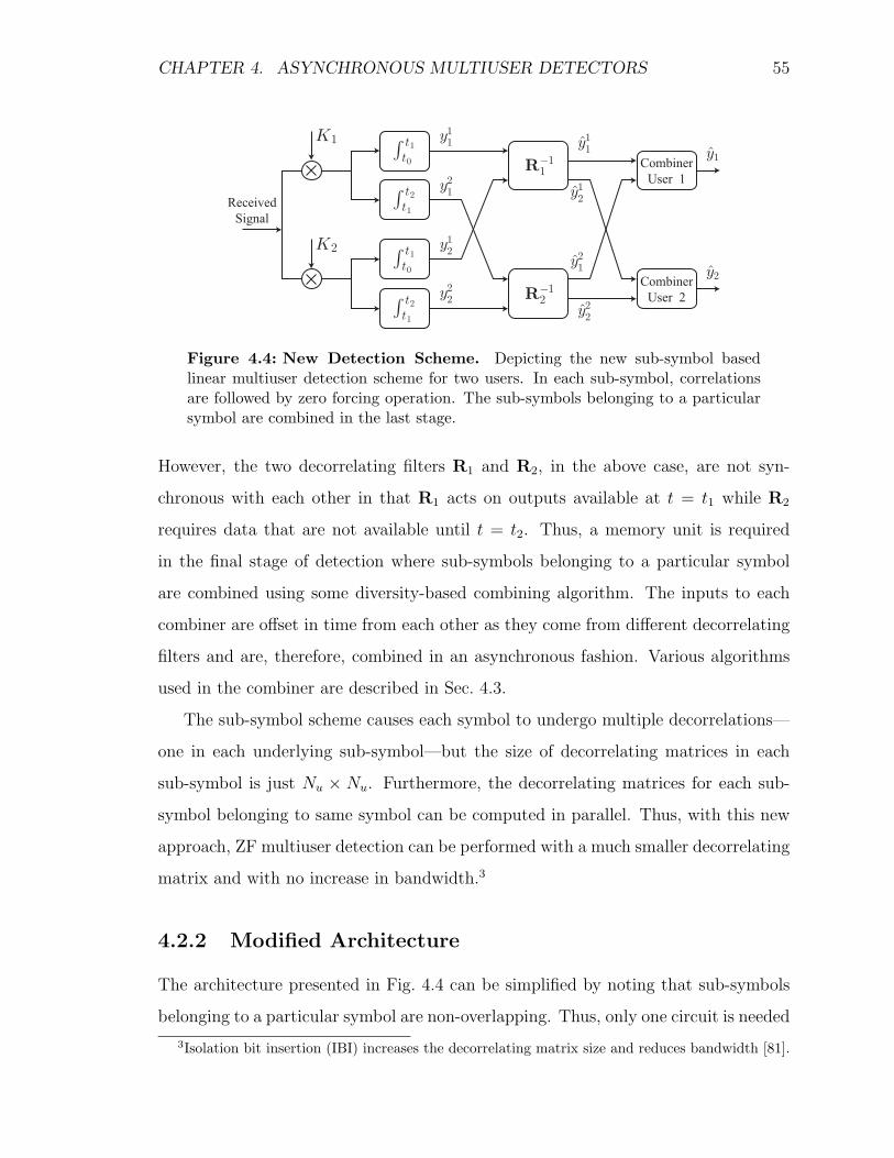
CHAPTER 4. ASYNCHRONOUS MULTIUSER DETECTORS 55
K1
K2
Rt1
t2
Rt1
t2
y11
y21
y12
y22
Rà1
1
Rà1
2
yê11
yê21
yê12
yê22
yê1
yê2
Combiner
User 1
Combiner
User 2
Received
Signal
Rt0
t1
Rt0
t1
Figure 4.4: New Detection Scheme. Depicting the new sub-symbol basedlinear multiuser detection scheme for two users. In each sub-symbol, correlationsare followed by zero forcing operation. The sub-symbols belonging to a particularsymbol are combined in the last stage.
However, the two decorrelating filters R1 and R2, in the above case, are not syn-
chronous with each other in that R1 acts on outputs available at t = t1 while R2
requires data that are not available until t = t2. Thus, a memory unit is required
in the final stage of detection where sub-symbols belonging to a particular symbol
are combined using some diversity-based combining algorithm. The inputs to each
combiner are offset in time from each other as they come from different decorrelating
filters and are, therefore, combined in an asynchronous fashion. Various algorithms
used in the combiner are described in Sec. 4.3.
The sub-symbol scheme causes each symbol to undergo multiple decorrelations—
one in each underlying sub-symbol—but the size of decorrelating matrices in each
sub-symbol is just Nu × Nu. Furthermore, the decorrelating matrices for each sub-
symbol belonging to same symbol can be computed in parallel. Thus, with this new
approach, ZF multiuser detection can be performed with a much smaller decorrelating
matrix and with no increase in bandwidth.3
4.2.2 Modified Architecture
The architecture presented in Fig. 4.4 can be simplified by noting that sub-symbols
belonging to a particular symbol are non-overlapping. Thus, only one circuit is needed
3Isolation bit insertion (IBI) increases the decorrelating matrix size and reduces bandwidth [81].

CHAPTER 4. ASYNCHRONOUS MULTIUSER DETECTORS 56
to compute the correlation product. Figure 4.5 depicts the modified architecture
for any number of users. In this case, only one integrator is used for each user
and the correlation product is dumped to the appropriate location at the end of
each sub-symbol. The switches used to dump the correlation products are controlled
by the acquisition and tracking circuit, which is assumed to have acquired correct
symbol timing. Furthermore, delay units are incorporated within the final combiner
in order to synchronize the inputs coming from different zero forcing decorrelators.
The amount of delay induced in each input of a combiner is again determined by the
acquisition and tracking block.
4.2.3 RAKE Implementation
RAKE receivers employ multiple detection fingers where each finger is a complete
SUMF detector [11], as described in Sec. 3.1.5. Signals at the output of different
RAKE fingers are combined using multipath diversity combining algorithms [43].
The new architecture described in Sec. 4.2.1 can be changed to represent a RAKE
receiver by simply removing the inverse filter blocks from Fig. 4.5 while considering
different RAKE fingers as individual users. The sum of signals generated as a result
of multiple sub-symbol correlations over a symbol is exactly the same as the signal
generated by one finger of a traditional RAKE. The combiner simply sums the signals
at its input and generates a signal corresponding to the signal at the output of one
RAKE finger. Thus, the new approach implements the RAKE receiver by remov-
ing ZF decorrelating filters, R−11 ,R−1
2 , . . . ,R−1Nu
from Fig. 4.5. Furthermore, different
combiners corresponding to a symbol and its multipath can jointly process the in-
formation now available at the granularity of sub-symbols. Although the processing
described above may lead to a better performance than that exhibited by a RAKE
receiver, it is beyond the scope of this thesis.

CH
AP
TE
R4.
ASY
NC
HR
ON
OU
SM
ULT
IUSE
RD
ET
EC
TO
RS
57
Received
signal
Combiner
user 1
Acquisition
and Tracking
Combiner
user Nu
Combiner
user 2
y11x
y21x
yNu
1x
y12x
y22x
yNu
2x
y2Nux
y2Nux
yNu
Nux
K1
K2
KNu
R
R
R
yê11x
yê21x
yêNu
1x
yê1
yê2
yêNu
Rà1
1
Rà1
2
Rà1
Nu
Figure 4.5: Sub-symbol Detection and Combining. Depicting the modified architecture for sub-symbol decorrelationand combining for Nu users. The outputs of the integrators are dumped at each sub-symbol boundary. Inputs to eachdecorrelating filter R−1
i come from those dump circuits whose outputs are available at the same time. The subscript “x”in the outputs indicates that the value is computed every symbol period. Inputs to each combiner are available at differenttimes and are synchronized by using delay units within the combiners.

CHAPTER 4. ASYNCHRONOUS MULTIUSER DETECTORS 58
4.2.4 Stability
The decorrelation matrix to perform the zero forcing operation is obtained by taking
the Moore-Penrose generalized inverse of the correlation matrix such as the ones
given in Eq. 4.5 and Eq. 4.6 [76]. If the correlation matrix is not badly scaled, the
ZF MUD remains optimally near-far resistant and the signals from different users can
be decorrelated successfully. In the case of badly scaled correlation matrix, however,
zero forcing operation can’t be performed and the performance reaches that of a single
user matched filter. Further, we note that a correlation matrix with high condition
number results in inferior BER performance of the ZF MUD as compared to an MMSE
MUD [78]. The proposed scheme is thus based on two thresholds as follows:
i) Chip Threshold (γc) which indicates that a sub-symbol should be processed
only if the size, in number of chips, of that sub-symbol exceeds this threshold.
This threshold is used to eliminate all instances in which the number of users
is greater than or equal to the number of chips in a sub-symbol.
ii) Condition Number Threshold (γn) which indicates that a particular sub-symbol
should not be processed if the correlation matrix during that sub-symbol is
badly scaled. This is used to avoid the cases of correlation matrix accidentally
becoming ill-conditioned even with large number of chips over which correlation
is performed.
As previously mentioned, asynchronism arises in wireless CDMA for two reasons:
random transmission instants and distances of users, and frequency selective fading.
The former is controllable while the latter has to be accounted for by the detection
scheme. Since the proposed scheme depends on the chip threshold, at those times
when, by chance, the symbols from some users are synchronous, the more chips are
likely to be in a sub-symbol and the better the scheme works. It is shown in Sec. 4.7
that the sub-symbol scheme needs only one “long” sub-symbol with an easily invert-
ible correlation matrix to essentially eliminate MAI. In the simulation of a general
CDMA system, we consider the worst case scenario for asynchronous users. That

CHAPTER 4. ASYNCHRONOUS MULTIUSER DETECTORS 59
is, no effort is made to synchronize the symbol starting instants which are taken as
independent and uniformly distributed over the symbol period. When the system is
synchronous with flat fading, there is just one sub-symbol per symbol, and the scheme
achieves the performance of the ZF MUD.
4.3 Combining algorithms
We now consider two sets of sub-symbol diversity combining algorithms: simple algo-
rithms, and condition number based algorithms.4 Simple algorithms are similar to the
ones used in RAKE receivers [11,43], the difference being that RAKE combining algo-
rithms operate on signals from different resolvable paths, while in the new scheme, the
combining is done for sub-symbols. Three simple algorithms for sub-symbol diversity
combining are as follows:
i) Select-best : In this algorithm the sub-symbol with maximum amplitude is se-
lected.
ii) Weighted : In this case, each sub-symbol is weighted by the strength of the
signal within that sub-symbol.
iii) Accumulate: This algorithm simply sums the signal in all the sub-symbols be-
longing to a particular symbol and the decision is made on the accumulated
result.
In addition to the simple combining algorithms, the sub-symbol architecture lends
itself to the definition of a new family of algorithms since the signals are obtained
from different sub-symbols which, unlike RAKE fingers, are obtained by performing
correlations over different numbers of chips. For example, in condition number based
combining algorithms, the three simple algorithms described above are modified such
4Another set of algorithms has been identified which uses the lengths of the sub-symbols whileperforming the combining. It was not pursued further due to inferior performance.

CHAPTER 4. ASYNCHRONOUS MULTIUSER DETECTORS 60
that each sub-symbol is weighted by the inverse condition number of the decorrela-
tion matrix during that sub-symbol. This idea is based on the result presented in [78]
where it is shown that the BER performance of ZF MUD deteriorates with the in-
creasing condition number of the correlation matrix.5 Such algorithms exhibit better
BER performance than simple combining algorithms as indicated by the results given
in Sec. 4.5.
4.4 Computational Complexity
The sub-symbol scheme allows detection of signals from various users in an asyn-
chronous CDMA channel with lower complexity than is required to implement previ-
ously known schemes. As stated earlier in the chapter, the scheme can also implement
a generalized RAKE receiver without requiring any matrix inversion. At first it may
appear that the scheme would require inverting a number of matrices per symbol as
large as the total number of users. In fact, simulations show that the addition of more
users to the system does not produce a linear increase in the number of matrices to
be inverted, but may actually decrease this number, at the cost of a BER penalty.
This occurs because adding a user to the system may cause a sub-symbol to be di-
vided into two sub-symbols such that none of them passes the chip threshold criteria.
While the complexity of many previously known schemes can be computed exactly,
the complexity of sub-symbol diversity combining scheme greatly depends upon the
thresholds selected and the relative asynchronism among users. Evaluation of the
exact value of computational complexity is not a performance-related issue and has
been scoped out of this thesis.
4.5 Performance Analysis and Results
Zero forcing linear MUD is known to completely suppress MAI and is optimally
near-far resistant [36, 70, 76, 78]. Because the sub-symbol scheme presented in the
5This result is also explained in Sec. 3.2.2.

CHAPTER 4. ASYNCHRONOUS MULTIUSER DETECTORS 61
-3 3 9 15 21 27 3310
-5
10-4
10-3
10-2
10-1
100
SNR in dB
Bit
Err
or R
ate
SUMFSelect-bestWeightedAccumulateIdeal ZF MUD
Figure 4.6: Simple Combining Algorithms. Performance comparison of threesimple combining algorithms with the SUMF and ideal synchronous ZF MUD.
previous sections employs the zero forcing principle in each sub-symbol to eliminate
MAI, it performs significantly better than a single user detector. The performance
margin between the new scheme and the single user detector depends upon the specific
combining algorithm used.
Figure 4.6 depicts the BER performance results for simple sub-symbol diversity
combining algorithms. These algorithms are similar to the ones used in combining
multipath diversity [11]. Of the three simple combining algorithms, the accumulate
algorithm exhibits the best BER performance, because it tends to average the noise
over the whole symbol. Since ZF MUD is known to perform poorly at low SNRs, the
three simple combining algorithms also show poor performance at low SNRs because
they are based on the zero forcing principle. Furthermore, Fig. 4.6 indicates that the
simple combining algorithms perform 4 dB to 8 dB worse than an ideal ZF MUD
used in completely synchronous system for uncoded BERs of 10−2 or better. That is,
the three algorithms require 4 dB to 8 dB higher SNR than that required by an ideal

CHAPTER 4. ASYNCHRONOUS MULTIUSER DETECTORS 62
ZF MUD to realize the same bit error rates.
An approximate expression for the performance loss with respect to ideal ZF MUD
can be derived for each of the simple combining algorithms. The derivation is greatly
simplified by assuming that fading imposes a fixed penalty6 in both cases: the ideal
ZF MUD case, and the case of simple combining algorithms. The fixed fading penalty
assumption allows the use of non-faded systems to compute the relative degradation in
BER for different receivers. The details of this computation are given in Appendix B.
Since the ZF MUD performance is dependent on the condition number of the
decorrelating matrix [78], it is possible to do better than the simple algorithms. This
is accomplished by using an algorithm that weighs the sub-symbols in inverse pro-
portion of the condition numbers of correlation matrices within those sub-symbols.
Figure 4.7 compares the BER performance of such an algorithm with that of a simple
accumulate combining algorithm. It can be seen that the condition number based
algorithm provides an approximate gain of 3 dB over the simple accumulate combin-
ing algorithm for 10−2 or better BERs. Condition number based algorithms exhibit
superior performance since they suppress those sub-symbols that lower the BER per-
formance due to badly scaled correlation matrices.
4.6 Near-Far Resistance with Sub-Symbol Scheme
The near-far problem arises when signals from mobile users reach the base station
with unequal powers. When this occurs, the signal from the user with the lowest
power is swamped out by the stronger interfering signals and thus suffers the highest
BER. It is well known that full symbol correlation based ZF MUD is the most near-
far resistant detector [36, 76]. To quantify the near-far resistance in terms of BER,
we performed simulations by placing one user, with weak signal, far from the base
station, and then noting the BER for this user while other users move progressively
closer to the base station. Average received power from the “far user” is fixed while
6Fixed penalty means that fading degrades the BER performance of each receiver in the sameway.
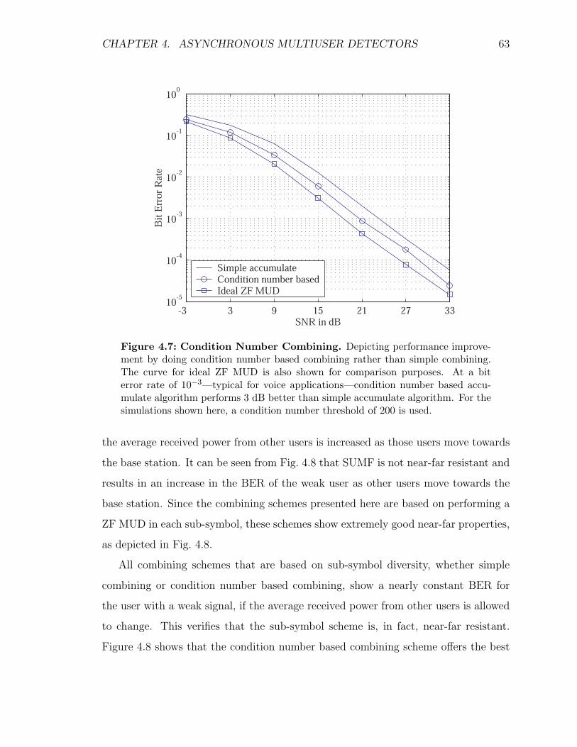
CHAPTER 4. ASYNCHRONOUS MULTIUSER DETECTORS 63
-3 3 9 15 21 27 3310
-5
10-4
10-3
10-2
10-1
100
SNR in dB
Bit
Err
or R
ate
Simple accumulateCondition number basedIdeal ZF MUD
Figure 4.7: Condition Number Combining. Depicting performance improve-ment by doing condition number based combining rather than simple combining.The curve for ideal ZF MUD is also shown for comparison purposes. At a biterror rate of 10−3—typical for voice applications—condition number based accu-mulate algorithm performs 3 dB better than simple accumulate algorithm. For thesimulations shown here, a condition number threshold of 200 is used.
the average received power from other users is increased as those users move towards
the base station. It can be seen from Fig. 4.8 that SUMF is not near-far resistant and
results in an increase in the BER of the weak user as other users move towards the
base station. Since the combining schemes presented here are based on performing a
ZF MUD in each sub-symbol, these schemes show extremely good near-far properties,
as depicted in Fig. 4.8.
All combining schemes that are based on sub-symbol diversity, whether simple
combining or condition number based combining, show a nearly constant BER for
the user with a weak signal, if the average received power from other users is allowed
to change. This verifies that the sub-symbol scheme is, in fact, near-far resistant.
Figure 4.8 shows that the condition number based combining scheme offers the best

CHAPTER 4. ASYNCHRONOUS MULTIUSER DETECTORS 64
0 3.9 7.78 13.0110
-2
10-1
100
Average Excess SNR of Strong Users [dB]
Bit
Err
or R
ate
SUMFSimple accumulateWeighted by sub-symbol lengthCondition number based
Figure 4.8: Near-Far Resistance. Comparing the near-far resistance of SUMFwith various sub-symbol combining methods. A constant BER indicates that sub-symbol combining methods are near-far resistant, while an increase in BER wheninterfering signals become stronger indicates that SUMF is not near-far resistant.Excess average SNR is the difference between average SNR in interfering signalsand the SNR in desired signal from the far user.
(i.e., lowest) BER and is completely near-far resistant. The simulations were per-
formed when the average SNR of strong interfering users exceeded the average SNR
of the far user by as much as 13 dB.
4.7 Maximizing System Capacity
This section focusses on fine tuning the sub-symbol technique to maximize the number
of simultaneous users for the combining algorithms described in Sec. 4.3. Here we
assume that moderate synchronism is achieved, as in a QS-CDMA system, by issuing
downlink commands to the users to adjust their transmission instants.
In previous sections it is assumed that user transmission is uncontrolled, which
implies that the starting instants of symbols received at the base station are uniformly

CHAPTER 4. ASYNCHRONOUS MULTIUSER DETECTORS 65
distributed over the entire symbol period. For a small number of users, the sub-
symbol intervals are long enough to allow easy decorrelation. But as the number of
users increases, the expected size of the sub-symbols becomes smaller, and it becomes
more difficult to perform ZF decorrelations within sub-symbols. When the number of
chips in a sub-symbol falls below the number of users, it is impossible to decorrelate
the signals of all the users in that sub-symbol successfully because the decorrelation
matrix always has one or more zero eigenvalues. In particular, if Nc is the number
of chips in a given sub-symbol, the maximum number of linearly independent users
in that sub-symbol is also Nc.7 When the actual number of users is greater than Nc,
the correlation matrix is singular and the signals within that sub-symbol can not be
completely decorrelated.
4.7.1 Types of Sub-Symbols
When the number of chips in a symbol is smaller than the total number of active
users, a regular inverse of the correlation matrix does not exist [76]. The same is
true for sub-symbols. In such cases, a generalized inverse or pseudo inverse has to be
used, while the condition number threshold γn is set to infinity. Towards this end, we
distinguish between two types of sub-symbols for a given user: a clean sub-symbol
indicating that the signal from this particular user has been successfully decorrelated
in this particular sub-symbol, and a corrupted sub-symbol which corresponds to one
of the zero eigenvalues of the correlation matrix.
When the correlation matrix is not of full rank, the maximum number of clean
sub-symbols is equal to the rank of the correlation matrix. Although one “long”
sub-symbol in which decorrelation can be performed is sufficient to bring the BER
down by a significant amount (see performance of select-best type simple combining
algorithm in Sec. 4.3), combining many clean sub-symbols brings down the SNR
penalty.8 Combining the corrupted sub-symbols with the clean sub-symbols, however,
7See [76] for details.8SNR penalty results from reduced processing gain; it is computed in Appendix B.
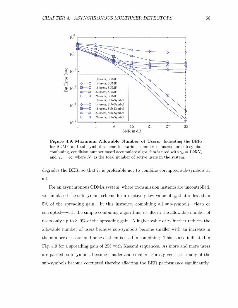
CHAPTER 4. ASYNCHRONOUS MULTIUSER DETECTORS 66
10 users, SUMF
14 users, SUMF
18 users, SUMF
22 users, SUMF
26 users, SUMF
10 users, Sub-Symbol
14 users, Sub-Symbol
18 users, Sub-Symbol
22 users, Sub-Symbol
26 users, Sub-Symbol
-3 3 9 15 21 27 33SNR in dB
10-5
10-4
10-3
10-2
10-1
100
Bit
Err
or R
ate
Figure 4.9: Maximum Allowable Number of Users. Indicating the BERsfor SUMF and sub-symbol scheme for various number of users; for sub-symbolcombining, condition number based accumulate algorithm is used with γc = 1.25Nu
and γn = ∞, where Nu is the total number of active users in the system.
degrades the BER, so that it is preferable not to combine corrupted sub-symbols at
all.
For an asynchronous CDMA system, where transmission instants are uncontrolled,
we simulated the sub-symbol scheme for a relatively low value of γc that is less than
5% of the spreading gain. In this instance, combining all sub-symbols—clean or
corrupted—with the simple combining algorithms results in the allowable number of
users only up to 8–9% of the spreading gain. A higher value of γc further reduces the
allowable number of users because sub-symbols become smaller with an increase in
the number of users, and none of them is used in combining. This is also indicated in
Fig. 4.9 for a spreading gain of 255 with Kasami sequences. As more and more users
are packed, sub-symbols become smaller and smaller. For a given user, many of the
sub-symbols become corrupted thereby affecting the BER performance significantly.
CHAPTER 4. ASYNCHRONOUS MULTIUSER DETECTORS 67
4.7.2 Sub-Symbol Scheme for QS-CDMA Systems
QS-CDMA systems, introduced in Sec. 3.1.1, reflect a moderately controlled environ-
ment in which users are instructed9 to adjust their transmission instants such that
their symbol arrival times at the base station fall within some fraction of the symbol
period. This kind of moderate synchronization is easier to implement than a fully
synchronized system.
For a QS-CDMA system employing sub-symbol detection, the thresholds for sub-
symbol decorrelation play an important role in determining the maximum number of
users that can be simultaneously accommodated in a QS-CDMA system employing
the sub-symbol scheme. The chip threshold γc is set sufficiently high such that only
one sub-symbol is used for demodulation. Use of such values for γc further reduces
the processing gain resulting in an SNR penalty, but if the signals from users can
be decorrelated successfully, simulations indicate that a significant improvement is
seen in BER for medium to high SNRs. For a QS-CDMA system with large number
of users, the sub-symbol combining system becomes the one that only uses selection
sub-symbol diversity since we consider only one dominant sub-symbol per symbol.
Thus, in this case, all the sub-symbol diversity combining algorithms converge to the
select-best sub-symbol combining algorithm. In this case, it is further known which
sub-symbol is selected for decorrelation in the select-best algorithm.
4.7.3 SNR Penalty for QS-CDMA Systems
The SNR penalty is defined as the degradation in SNR that results from partial-
period correlations instead of full period correlations. It is, therefore, the result of
reduced processing gain of the sub-symbol scheme. The SNR penalty for select-best
algorithm is derived in Appendix B and is given by NM
, where N is the total number
of chips per symbol and M is the number of chips used to perform partial-period or
sub-symbol correlation. This penalty can be reduced if fewer users are present and
more sub-symbols can be combined. If the system is moderately synchronized, as in
9Sending commands on the downlink can accomplish this.

CHAPTER 4. ASYNCHRONOUS MULTIUSER DETECTORS 68
P = 64 P = 128 P = 192
Nu = 10 196.86 139.26 81.65
Nu = 30 192.66 130.77 68.90
Nu = 50 191.83 129.08 66.35
Nu = 70 191.50 128.37 65.27
Nu = 90 191.32 127.98 64.67
Table 4.1: Expected number of chips in a sub-symbol.
case of QS-CDMA, and the users are allowed to have their transmission instants lie
within the first P chips of a reference symbol,10 then the expected value of M is given
by:
E[M ] = (N − P ) +P−1∑i=0
{i(αi − αi+1)
}+ PαP
= (N − P ) +α − αP+1
1 − α
(4.7)
where α is defined as:
α ≡(
P − 1
P
)Nu
(4.8)
For practical reasons, P is a large fraction of N , typically ranging from 50% to 80%.
In such cases, the expected value of M for a large number of users is approximately
given by N − P ; for N = 255, exact expected value of M is listed in Table 4.1.
4.8 Threshold Optimization
For the decorrelation process in each sub-symbol, either the regular inverse, which we
will denote by �, or the generalized inverse, denoted by ℘, is used. We consider the
effect of thresholds in each case. The condition number threshold γn is important only
if the � operation is performed and does not have any significance for the ℘ operation.
As long as the number of chips in a sub-symbol is less than the number of users in that
sub-symbol, the � operation can not be performed. Thus, the performance of the �10Also see Sec. 3.1.1.

CHAPTER 4. ASYNCHRONOUS MULTIUSER DETECTORS 69
operation becomes independent of γc when γc is less than the number of users. As the
number of users increases, it may not be possible to perform the � operation at all
and the ℘ operation is the only recourse. In such a case, a small value of γc results in
more and more sub-symbols being considered for decorrelation, which increases the
probability of contamination of clean sub-symbols by the corrupted sub-symbols.
For a given γc, increasing the number of users brings two benefits: more users are
accommodated, and there is less chance for a corrupted sub-symbol being considered
for combining with closely packed users. Therefore, when transmission instants of
users can be bound within a small region, a value of γc exceeding the length of that
region is desirable. Otherwise, with fewer users, it is better to use the � operation.
When the ℘ operation is used, it is ensured that in each sub-symbol there are
enough chips to decorrelate the signals from various users. If there are many corrupted
sub-symbols and fewer clean sub-symbols in a sub-symbol interval, it is advantageous
to isolate all the sub-symbols in that interval without using them in sub-symbol
combining. Obviously, the ideal situation is to be able to pick the sub-symbols for
only those users that have been decorrelated successfully. If it is not possible to
selectively pick users from within a sub-symbol, the chip threshold γc should be
selected such that there is a good chance for most of the users to be decorrelated.
Thus as the number of users increases, a larger value of γc is needed, up to a certain
limit, after which it should be set to a constant value such that we have at least one
sub-symbol to carry out the decorrelation process.
An alternate measure for performance adjustment is the rank threshold γr, which
indicates that the decorrelation operation is performed in a sub-symbol if the corre-
sponding correlation matrix has a rank that exceeds γr. We consider following two
cases for a QS-CDMA system:
i) Number of users is small such that Nu Nc for all sub-symbols. In this case, γr
is made equal to the number of active users. Furthermore, either γc or γn is used
in conjunction with γr. The possibility of combining corrupted sub-symbols is
reduced by using one of the following two strategies:

CHAPTER 4. ASYNCHRONOUS MULTIUSER DETECTORS 70
Pseudo Inverse (℘) Regular Inverse (�)
γn = 200 γn = 500
P = 128; γc = 0.25Nu 117 97 110
P = 192; γc = 1.00Nu 62 51 53
Table 4.2: Maximum number of supported users. The numbers shown are de-
termined when the conditions in the table result in a BER that is an order of
magnitude less than the BER exhibited by an SUMF at an SNR of 30 dB.
(a) Choose γc slightly larger than Nu; by using much higher values for γc, we
run the risk of not considering an interval in which all the sub-symbols are
clean. For γc < Nu, we do not avoid combining of corrupted sub-symbols.
(b) Choose γn in the medium range; lower values run the risk that clean sub-
symbols will not be combined, and higher values do not avoid combining
of corrupted sub-symbols.
ii) Number of users is very large. Under this condition, we have only one sub-
symbol available that needs to be decorrelated and a value of γr slightly smaller
than the number of users would be the right choice.
Table 4.2 depicts the maximum number of users in a moderately synchronized
system with a spreading gain of 255. The maximum number of supported users
shown in this table is determined by the criteria that the sub-symbol detector results
in a BER that is at least an order of magnitude better than the single user matched
filter receiver at a signal-to-noise ratio of 30 dB.
4.9 Recap
This chapter presents a sub-symbol based computational scheme for linear multiuser
detection in a DS-CDMA system. This scheme facilitates decorrelating the undesired
signals from the received signal at the base-station receiver. Further, it keeps the
linear decorrelating filter computationally tractable while accommodating the asyn-
chronicity of users created by random transmission instants and multiple resolvable

CHAPTER 4. ASYNCHRONOUS MULTIUSER DETECTORS 71
paths. Unlike previous multiuser detection schemes for asynchronous systems, this
scheme does not depend on the number of symbols in the duration of transmission
and it does not reduce the symbol transmission rate.
The sub-symbol scheme uses a new kind of diversity which we call sub-symbol
diversity. Algorithms for diversity combining of sub-symbol are also presented in this
chapter. Simulations confirm that the sub-symbol scheme is near-far resistant and
performs significantly better than a SUMF detector.
The new scheme also represents an alternate construction of the RAKE receiver
where reduction in multiple access interference (MAI) is not the primary objective.
In such a case, signals from users are not decorrelated within sub-symbols and the
sub-symbol diversity combiner is used as a multipath diversity combiner.
Though the application of sub-symbol method to asynchronous systems improves
the BER for all users, it still limits the maximum number of users and, therefore,
does not improve the system capacity significantly. When the sub-symbol method
is applied to a QS-CDMA system, however, system capacity improves and the total
number of users accommodated in such a system is given roughly by the length, in
number of chips, of the longest sub-symbol. In QS-CDMA systems, when the appro-
priate values for the chip and condition number thresholds are used, the “select-best”
sub-symbol scheme can support a maximum number of users that is approximately
given by the maximum number of chips in any sub-symbol. For example, if the longest
sub-symbol is 63 chips long, irrespective of the spreading factor, the maximum num-
ber of users supported is approximately 63. In this case, for each user, the sub-symbol
based MUD yields a BER that is at least an order of magnitude better than a SUMF
detector.

Chapter 5
Multiple Antenna Systems
This chapter presents signal processing and communication techniques that make use
of multiple antennas at the transmitter and the receiver. The use of multiple an-
tennas for wireless communications produces significant performance improvements,
including the reduction of bit error rates and the increase of capacity. These improve-
ments allow more users to access the system with higher data rates for the same bit
error rates than is the case of single antenna. How multiple antenna systems can be
combined with linear multiuser detectors to enhance the performance of a DS-CDMA
system is the subject of this chapter.
“Beamforming” and “adaptive array processing” are terms used primarily to refer
to the use of multiple receiving antennas in a mobile communication system. To avoid
confusion, however, it should be noted that beamforming is used to also refer to the
use of multiple transmitting antennas at the base stations in fixed wireless systems.1
For the purpose of the discussion of the mobile DS-CDMA environment, we restrict
the use of these terms to a system with multiple receiving antennas.
While beamforming (BF) with multiple receiving antennas significantly improves
the BER performance, it fails to suppress multiple access interference, resulting in an
irreducible BER floor. Adding channel encoding at the transmitter and soft-decision
Viterbi decoding (VD) at the receiver further lowers the BER floor. Furthermore,
1Fixed wireless systems can be cellular or non-cellular and have the constraint that the end usersare not mobile.
72

CHAPTER 5. MULTIPLE ANTENNA SYSTEMS 73
a combination of BF and linear MUD results in effective elimination of MAI while
maintaining better BERs at low SNRs.
This chapter provides the vector channel model that characterizes a wireless sys-
tem with multiple antennas. It also presents simulation results for the case of multiple
receiving antennas with one dominant path from each mobile user. Such results depict
the effect of using multiple receiving antennas in a wireless communication systems.
The simulations performed are for a DS-CDMA system with specifications as given in
some of the proposed WCDMA standards [63]. We demonstrate that it is preferred
to define the “performance gain” achieved by multiple antenna system in terms of
improvement in BER rather than as a decrease in required SNR. We further argue
that such definition of performance gain is applicable to most communication systems
that exhibit a BER floor.
5.1 Background
All multiple access systems employ some form of filtering at the receiver to recover
the desired signal. In an FDMA system, a receiver rejects the undesired signals and
recovers the desired signal by passing the composite signal through a narrowband
filter. In TDMA, time selection is achieved based on the knowledge of time frames
during which signals from different users are received. In CDMA, “code-matched”
filtering or correlation detection is performed to recover the desired signal whilst at-
tenuating the other undesired signals. Multiple antennas (or an antenna with multiple
elements) provide a means of performing spatial filtering which offers increased signal-
to-interference-plus-noise ratio (SINR) by increasing the relative antenna gain in the
direction of the desired user. The notion of spatial filtering is, therefore, synonymous
with beamforming, where the tap weights dictate the antenna gain pattern.

CHAPTER 5. MULTIPLE ANTENNA SYSTEMS 74
5.1.1 Classification of Multiple Antenna Systems
From a signal processing point of view, systems using multiple antennas can be
broadly classified into three different categories:
i) Systems in the first category use multiple receiving antennas with one path
from each transmitting handset in a multiple access channel. In such systems,
array signal processing algorithms are used to combine signals from different
receiving antennas. These algorithms and the conditions under which they are
applicable are specified later in the chapter.
ii) In the second category, the receiver has multiple antennas with the possibility
of multiple paths from each mobile user. In this case, array signal processing
needs to be combined with processing in time—the combination is referred to
as space-time (ST) processing. Although ST processing can be used at the
transmitter as well as at the receiver, the term is generally used to describe
the processing at the receiver. The ultimate goal is to equalize the multiuser
channel thereby combating channel impairments that include multipath fading,
co-channel interference (CCI), delay spread, and thermal noise.
iii) The third category of systems uses multiple antennas at both the transmitter
and the receiver. This enables the use of ST processing at the receiving end and
space-time coding at the transmitting end. This is the most common situation
of using multiple antennas in a mobile communication system.
Another important, and sometimes overlooked, way of classifying the multiple an-
tenna systems is by considering the spacing between antenna elements. This spacing
between the elements is very important for ST processing (at the receiver) or ST
coding (at the transmitter) as it gives an idea of the correlation between the signals
at different antenna elements. The farther the elements are spaced, the lower is the
correlation between the signals received at each antenna element. When the elements
are sufficiently spaced, the signal decorrelates from one element to the other. That

CHAPTER 5. MULTIPLE ANTENNA SYSTEMS 75
is, signals at different elements undergo uncorrelated fading. In such an instance,
signals from different elements can be combined to realize a form of diversity called
antenna diversity. Therefore, multiple antenna systems can be viewed as providing
one or both of the following gains:
i) Diversity gain, which is achieved if individual elements are widely spaced and
undergo uncorrelated fading. Diversity gain allows a reduction in average output
SNR per antenna for a given bit error rate.
ii) Directional gain, which is achieved when the elements are closely placed. This
gain, also called directive gain, signifies the reduction in required received signal
power for a given output SNR.
Element spacing that achieves uncorrelated fading is generally a complex function
of the signal frequency and propagation environment [85]. The most important en-
vironmental factor that effects the required element spacing for signal decorrelation
is the angular spread:2 the smaller the angular spread, the farther the elements need
to be placed for the received signals to fade independently [87]. Thus, the require-
ment for signal decorrelation at different elements leads to large antenna sizes in such
environments that exhibit small angular spread (for example, base stations mounted
on the top of the buildings). In such instances, where angular spread is small and
antenna size is limited, diversity gain may not be realized because of correlated fad-
ing on individual antenna elements. Still, the directional gain makes use of multiple
antennas an attractive choice. In fact, smaller angular spread results in larger di-
rectional gain by using multiple antennas, so that the two types of gains realized by
multiple antenna systems tend to compensate for one another’s deficiencies.
2Estimation of angular spread is accomplished by means of super resolution techniques. See [86]for details.

CHAPTER 5. MULTIPLE ANTENNA SYSTEMS 76
5.2 Beamforming Mechanism
The beamforming mechanism is described by means of an array response vector and
a beamformer tap weight vector (i.e., tap weights in the spatial filter). In order to
appreciate the benefits of spatial filtering, consider two users and a receiving antenna
with two elements. If v11 and v21 are the antenna gains for user-1 at the two elements
while v12 and v22 are those for user-2, then the array response vectors for the two
users are expressed as [v11 v21]T and [v12 v22]
T , where [·]T denotes the transpose.
For the two user and two antenna example, there is one beamformer for each user.
The beamformer for the 1st user simply provides a beamformer tap weight vector
�w∗1 = [w∗
11 w∗21], where asterisk in the superscript denotes the conjugate of a scalar.
For the two users, overall gains obtained from this beamformer are:
For user-1: Gain is g11 = w∗11v11 + w∗
21v21
For user-2: Gain is g12 = w∗11v12 + w∗
21v22
To suppress the signal from user-2, we need g11 > g12, which can be achieved by
a judicious choice of �w∗1. Specifically, consider a user whose angle of arrival (AOA) is
θ at a uniform linear array, as shown in Fig. 5.1. The array is assumed to have Nm
similar elements with element spacing d. In the case of a planar wavefront, the path
difference between two consecutive elements is d sin θ, such that the corresponding
phase difference is as follows [88]:
φ = d sin θ(2πfc
c
)= 2π sin θ
(d
λ
)(5.1)
where fc is the carrier frequency, λ is the wavelength, and c is the velocity of the
incident wave.
The array response vector is an indication of how an array responds to a signal.
For a single AOA, the array response vector is given by:
[v0 v0e
−jφ v0e−j2φ · · · v0e
−j(Nm−1)φ
]T
(5.2)

CHAPTER 5. MULTIPLE ANTENNA SYSTEMS 77
dsin
θ
θ
d
Figure 5.1: Single AOA at Multiple Receiving Antennas. A uniform lineararray is demonstrated here on which radio signal falls from a single angle. Generally,the signal received at the array comes with some angular spread, even when thereis a single transmission source; the amount of angular spread depends upon thepropagation environment.
which indicates that the array response vector is a function of d, λ, and θ: the
array response vector can be evaluated by determining the antenna spacing and the
frequency and AOA of the incident wave. In the above expression, taking v0 = 1
without loss of generality, the array response vector becomes:
[1 e−jφ e−j2φ · · · e−j(Nm−1)φ
]T
(5.3)
If �v1 is the array response vector for the 1st user and �v2 for the 2nd user, then the
beamformer for user-1 selects �w∗1 such that:
|�w∗1�v1| ≥ |�w∗
1�v2| (5.4)
5.2.1 Beamforming Algorithms
Various beamforming algorithms exist for choosing the tap weight vector and each of
these algorithms are based on different criteria. The simplest algorithm, in which the

CHAPTER 5. MULTIPLE ANTENNA SYSTEMS 78
weight vector is selected to be the conjugate transpose of the array response vector,
is called the delay-and-sum algorithm [89]. It simply compensates for the different
delays incurred by the impinging signal at different antenna elements. While it is the
simplest of all algorithms, it is not optimal in all the situations. Other beamforming
techniques, based on more sophisticated algorithms, exist and have been discussed
in [88] and [89].
In our simulations, an array with Nm = 4 and d = λ is used. We assume a narrow
angle of arrival that can be estimated fairly accurately, such that the spatial fading
over the antenna elements can be neglected [86, 88]. Under such conditions, another
beamforming algorithm, the max-SINR algorithm, can be used effectively. In the
max-SINR algorithm, the conjugate transpose of tap weight vector is selected such
that the SINR is maximized. The tap weight vector for SINR maximization is derived
in [88] and is given by the following:
�wi = Ruu,i�vi (5.5)
where �vi is the array response vector as before, and Ruu,i is the correlation matrix of
the undesired signal for i-th user. Therefore, Ruu,i can be written as [88]:
Ruu,i =Nu∑j=1j �=i
(σ2
BPSKR2ijE[AjA
∗j ]�vj�v
∗j
)+ Nσ2
nI (5.6)
5.2.2 Transmitter Analysis and Vector Channel
Let us now consider modelling a system with single transmitting antenna. The trans-
mitter model, which is independent of the number of receiving antennas, is essentially
the same as described in Chapter 2. The channel model, however, changes with the
number of receiving antennas. Let the i-th user be incident with angle θi. From
Eq. 5.3 and Eq. 5.1, the array response vector for the i-th user, denoted as �vi, can be
written as:
�vi =[1 e−j2π
dSinθiλ e−j4π
dSinθiλ · · · e−j(Nm−1)2π
dSinθiλ
]T
(5.7)

CHAPTER 5. MULTIPLE ANTENNA SYSTEMS 79
Using the notation such that vij denotes the elements of �vi, the array response
vector for the i-th user can be written as:
�vi =[v1i v2i · · · vNmi
]T
(5.8)
The vector channel or the array response matrix V for all the users is, therefore,
given by:
V =
v11 v12 · · · v1Nu
v21 v22 · · · v2Nu
......
. . ....
vNm1 vNm2 · · · vNmNu
(5.9)
where Nu is the number of active users as before.
5.2.3 Receiver Analysis
The receiver is assumed to have Nm antenna elements and the signal received is a
vector signal with Nm dimensions. The “signal+interference” portion of the received
signal given in Eq. 2.14 passes through the vector channel and is scaled by the array
response vectors. The gaussian “noise” portion, however, remains intact because
noise is assumed to be added at the antenna elements.
If ri is the signal received from antenna-i, then the received vector signal is:
�r =
r1
r2
...
rNm
=
v11K1A1d1 + v12K2A2d2 + · · · + v1NuKNuANudNu
v21K1A1d1 + v22K2A2d2 + · · · + v2NuKNuANudNu
...
vNm1K1A1d1 + vNm2K2A2d2 + · · · + vNmNuKNuANudNu
+ �nant
(5.10)
where the correlation matrix of �nant is Rnantnant = σ2nINm .
At the receiver, there are two options: “beamform” first and then “despread”, or
despread first and then beamform.3 In linear systems, these options are equivalent
3The term despread is used to denote the process of correlating the received spread spectrum

CHAPTER 5. MULTIPLE ANTENNA SYSTEMS 80
Ante
nna-1
Ante
nna-2
Ante
nna-N
m
K1
K2
KNu
K1
K2
KNu
K1
K2
KNu
w∗11
w∗21
w∗Nm1
w∗11
w∗21
w∗Nm1
w∗11
w∗21
w∗Nm1
y(1)arr
y(2)arr
y(Nu)arr
∑
∑
∑
Beamformer-1
Beamformer-2
Beamformer-Nu
∫symbolperiod∫symbolperiod
∫symbolperiod
∫symbolperiod∫symbolperiod
∫symbolperiod
∫symbolperiod∫symbolperiod
∫symbolperiod
Figure 5.2: Multiple Antenna Receiver-I. Despreading prior to beamforming.
to one another. Two schemes based on these options are shown in Fig. 5.2 and
Fig. 5.3. It is more cost-effective to despread first and then beamform, since in this
case beamforming is performed at the symbol rate instead of at the chip rate.
CDMA signal with the spreading sequence. The term beamform denotes the process of combiningthe signals from multiple antennas.

CHAPTER 5. MULTIPLE ANTENNA SYSTEMS 81
1
2
Nm
w∗11
w∗21
w∗Nm1
w∗11
w∗21
w∗Nm1
w∗11
w∗21
w∗Nm1
∑
∑
∑
K1
K2
KNu
y(1)arr
y(2)arr
y(Nu)arr
Beamformer-1
Beamformer-2
Beamformer-Nu
∫symbolperiod
∫symbolperiod
∫symbolperiod
Figure 5.3: Multiple Antenna Receiver-II. Beamforming prior to despreading.
The gain provided by the i-th beamformer to the signal of the j-th user is given
by:
gij = �w∗i �vj (5.11)

CHAPTER 5. MULTIPLE ANTENNA SYSTEMS 82
where �w∗i is the conjugate transpose of �wi. The objective is to select �w∗
i such that:
gii ≥ gij, ∀j �= i (5.12)
After despreading and beamforming, the received signal for the i-th user can be
written as:
y(i)arr = giiRiiAidi +
Nu∑j=1j �=i
(gijRijAjdj
)+ n(i)
arr (5.13)
Comparing Eq. 5.13 with Eq. 3.3 and neglecting the additive noise terms, we
observe a significant improvement in �yarr over �y since a judicial choice of �w∗i ensures
gii ≥ gij, ∀j �= i. Furthermore, the spreading sequences are selected such that
Rii � Rij, ∀j �= i. Hence:
giiRii � gijRij, ∀j �= i (5.14)
Equation 5.14 indicates that the undesired or MAI components are attenuated
as compared to the desired component. Simulation results, assuming random AOAs
for each user’s signal, are given in Fig. 5.4. These results demonstrate that multiple
antenna systems perform significantly better than a single antenna system. Though
a BER floor is still observed, it is lower for systems with multiple antennas than it
would be for a single antenna system.
The use of channel encoding with multiple antennas results in further improvement
in performance, as indicated in Fig. 5.5. However, a BER floor is again noticed since
channel encoding is not designed to mitigate the MAI.
The two beamforming algorithms stated in Sec. 5.2.1—delay-and-sum and max-
SINR—perform equally well for uniformly distributed users. This is because uni-
formly distributed users appear approximately spatially “white”, and thus the cor-
relation matrix of the undesired signal, Ruu,i, is also approximately uniform. Under
this condition, the weight vector obtained from SINR maximization criterion is the
same as the one obtained from delay-and-sum criterion [88].

CHAPTER 5. MULTIPLE ANTENNA SYSTEMS 83
-3 0 3 6 9 12 15 18 21 24 2710
-4
10-3
10-2
10-1
100
SNR in dB
Bit
Err
or R
ate
1 Antenna2 Antennas4 Antennas6 Antennas8 Antennas
Figure 5.4: BER Performance with Multiple Antennas. Performance Im-provement with Multiple Antennas for Nu = 12 users and Flat Rayleigh Fading.Delay-and-sum beamforming is used with SUMF to obtain these curves.
When the angular distribution of users is not spatially uniform, as is the case
for a 30◦ sector, max-SINR beamformer performs better than the delay-and-sum
beamformer. Simulation results shown in Fig. 5.6 confirm this.
5.3 Multiple Transmitting Antennas
Beamforming at the receiver is well understood and several researchers have addressed
the topic of ST processing at the receiver [87, 88]. Furthermore, diversity techniques
using multiple receiving antennas are also discussed in several textbooks [11, 22, 43].
Use of multiple transmitting antennas and ST coding at the transmitter, however,
represent a relatively new research area. In this section, we summarize the perfor-
mance gains achieved by using multiple transmitting antennas. When both transmit-
ter and receiver use multiple antennas, the performance improvement depends upon
the number of receiving antennas used in the system.

CHAPTER 5. MULTIPLE ANTENNA SYSTEMS 84
-3 0 3 6 9 12 15 18 21 24 2710
-6
10-5
10-4
10-3
10-2
10-1
SNR in dB
Bit
Err
or R
ate
SUMFSUMF + VD
Figure 5.5: Multiple Antennas with Channel Encoding. Performance im-provement with channel encoding in a four-antenna receiver (i.e., Nm = 4) forNu = 12 users. The results with channel encoding are obtained by using a Viterbidecoder at the receiver and an encoder at the transmitter. The encoder used is aconvolutional encoder with rate 1
2 and constraint length 5.
Multiple transmitting antennas provide a form of diversity known as space di-
versity.4 There are situations when space diversity is the only choice because it is
not possible to use other types of diversity under all conditions. For example, the
presence of small values of delay spread prohibits RAKE combining (or multipath
diversity) in DS-CDMA systems. Similarly time diversity can not be used in slowly
fading channels, especially if the data are delay constrained [90].
Beamforming using multiple transmitting antennas is based on the same vector
channel model described in Sec. 5.2.2 for multiple receiving antennas. Transmit di-
versity schemes can be of three types: feedback assisted, training assisted, and blind.
The capacity regions using transmit diversity have been discovered previously [90],
but practical schemes are still being investigated. The delay diversity scheme [91] is
a very simplified form of transmit diversity in which two transmitting antennas are
4In the literature, space diversity is also referred to as transmit diversity.

CHAPTER 5. MULTIPLE ANTENNA SYSTEMS 85
-9 -6 -3 0 3 6 910
-5
10-4
10-3
10-2
10-1
SNR in dB
Bit
Err
or R
ate
Delay-and-sum algorithmMax-SINR algorithm
Figure 5.6: Comparison of Beamforming Algorithms. Two beamformingalgorithms, delay-and-sum and max-SINR, are compared for a 30◦ sector. Thecurves are obtained for a system with Nm = 4 antennas and Nu = 12 users in flatRayleigh fading.
used and the same symbol sequence is transmitted from each with a delay of one
symbol between the two antennas. As a consequence, this scheme prevents the loss
of data rate while providing a dual branch diversity reception at the receiver using
maximum likelihood sequence estimation (MLSE). It can be demonstrated that the
capacity grows linearly with the number of transmitting antennas under the condition
that the number of transmitting antennas remains less than the number of receiving
antennas [90]. Considering n transmitting antennas and m receiving antennas, where
the gain from antenna i to antenna j is assumed to be slowly varying, then for BPSK
in Rayleigh fading, the average probability of symbol error is given by [90]:
Pe ≤(
1∏ni=1(1 + λiEs/4No)
)m
(5.15)
where λi denotes the i-th eigenvalue of error covariance matrix [90]. If the error
covariance matrix has r non-zero eigenvalues (that is, it has a rank r), then the above

CHAPTER 5. MULTIPLE ANTENNA SYSTEMS 86
inequality can be written as:
Pe ≤( r∏
i=1
λi
)−m(Es
4No
)−rm
(5.16)
Comparing this with the standard expressions for error probability as given in [22]
and [43], a diversity gain of mr and a coding gain of (λ1λ2 · · ·λr)1/r is achieved. The
criterion for the selection of ST codes for transmit diversity in Rayleigh and Rician
fading have been reported in [90].
ST coding, which fundamentally addresses transmit diversity, can be combined
with array processing in order to reduce the decoding and encoding complexity of
the transmitter and receiver that results by using ST codes. Decoding complexity
exponentially increases with the decoding rate for a fixed number of transmitting
antennas [92]. A linear array processing technique at the receiver, described in detail
in [92], can be used in conjunction with ST coding. This technique, called the group
interference suppression method, works by assuming that the signals transmitted from
other groups of antennas are interference and tries to cancel out such interference.
5.4 Performance Gain
In this section, we provide a definition of the performance gain of multiple antenna
system over single antenna system. This definition is applicable to any communication
system that exhibits BER floor, such as a wireless DS-CDMA system.
Figure 5.4 shows that the DS-CDMA system exhibits BER floor like many other
communication systems. The reasons for BER floor for different communication sys-
tems are quite different. For example, TDMA systems exhibit an error floor due to
ISI. But systems using differential modulation exhibit a BER floor due to doppler
spread [43]. The BER floor in DS-CDMA systems is the result of multiple access
interference. This floor is observed irrespective of the number of receiving antennas
because beamforming with multiple receiving antennas can not completely eliminate

CHAPTER 5. MULTIPLE ANTENNA SYSTEMS 87
multiple access interference for the DS-CDMA systems. However, use of multiple
receiving antennas results in a reduction in BER floor.
The performance gain for any performance improvement scheme is usually defined
as the reduction in required SNR for a given BER. Referring to Fig. 5.4, this definition
can not be applied to beamforming performance gain because a specified BER may
never be achieved by the system if the number of antennas is too small. An alternate
measure of equal significance is the reduction in BER at a given SNR. This definition
is most effective in the floor region. Thus, we define the performance gain of a
beamforming scheme as the ratio of BER floor for multiple antennas to the BER
floor for single antenna. That is, if G(m) is the gain by using m antennas, we can
write:
G(m) =BER floor with m antennas
BER floor with one antenna(5.17)
We also note from Fig. 5.4 that G(m) does not increase linearly with m, and increasing
the number of receiving antennas brings diminishing returns in gain.
5.5 Linear MUD with Multiple Antennas
In Chapter 3, we demonstrate that use of linear multiuser detectors improves system
performance. Furthermore, as given in earlier sections, use of multiple antennas in
a DS-CDMA systems results in a reduction in BER floor, a second improvement.
When multiple antennas are used with linear multiuser detectors, the resulting sys-
tem enables further improvements in system performance. This section describes a
combination of multiantenna systems and linear multiuser detectors.
It has been established in previous chapters that beamforming and linear mul-
tiuser detection combat multiple access interference, but perform poorly in certain
SNR regions. Specifically, ZF linear MUD performs poorly for low SNRs, while a
multiple antenna system with SUMF exhibits a BER floor at high SNRs. In Chap-
ter 3, we demonstrated that linear multiuser detectors are extremely near-far resistant
and robust against MAI originated within local cell. Further, Sec. 5.2 depicts that

CHAPTER 5. MULTIPLE ANTENNA SYSTEMS 88
beamforming is more robust against unknown MAI that originates from other cells.
Thus, a combination of the two schemes, namely linear MUD with beamforming,
offers substantial gains, as pointed out in [93] based on architecture proposed in [94].
Simulation results suggest that for various voice and data applications, a combina-
tion of linear multiuser detector and beamformer outperforms either the beamformer
or the multiuser detector alone. Voice applications generally require a BER of 10−3
or better, while BER requirements for data applications are more stringent, lying in
the range of 10−6 or better. A receiver that uses ZF linear MUD with BF is shown in
Fig. 5.7. At each element of the antenna array, individual users are first despread, then
decorrelated via the R−1 filter, and then beamformed individually. Such an approach
completely eliminates MAI at high SNRs while affording an adequate performance at
lower SNRs, as shown in Fig. 5.8.
5.5.1 ZF MUD with Beamforming
In a multiple antenna receiver system, performing the decorrelation operation at each
antenna renders the statistical signal spatially white at the input of the beamformer.
To prove this, it suffices to show that when ZF or decorrelator MUD is used at each
antenna element then the correlation matrix of the undesired signal present at the
input of each beamformer is spatially white [93], irrespective of the sector size.
The heuristics of the proof are as follows: Since the beamformer for a particular
user receives the input signals from different antennas, the unwanted signal that causes
non-zero spatial correlation is MAI and not the additive gaussian noise.5 In Fig. 5.8,
without decorrelating operation at each antenna, we would expect spatial correlation
due to the presence of MAI in the signals coming from each of the antenna. However,
the use of a decorrelating filter leaves only additive gaussian noise as the unwanted
signal uncorrelated with the additive gaussian noise on any other antenna element,
thereby rendering the unwanted signal spatially white. The formal proof is provided
5This follows from the assumption that the additive gaussian noise at one antenna is uncorrelatedwith the noise at any other antenna.

CHAPTER 5. MULTIPLE ANTENNA SYSTEMS 89
Ante
nna-1
Ante
nna-2
Ante
nna-N
m
K1
K2
KNu
K1
K2
KNu
K1
K2
KNu
w∗11
w∗21
w∗Nm1
w∗11
w∗21
w∗Nm1
w∗11
w∗21
w∗Nm1
y(1)com
y(2)com
y(Nu)com
∑
∑
∑
Beamformer-1
Beamformer-2
Beamformer-Nu
R−1
R−1
R−1
∫symbolperiod∫symbolperiod
∫symbolperiod
∫symbolperiod∫symbolperiod
∫symbolperiod
∫symbolperiod∫symbolperiod
∫symbolperiod
Figure 5.7: Multiantenna with linear MUD. A multiantenna ZF multiuserdetector. The zero forcing or decorrelation operation is performed at each antennaindividually and the signals are combined later using a beamformer for each user.
below:
The received vector signal from Eq. 5.10 is written as:
�r = K1A1d1�v1 + K2A2d2�v2 + · · · + KNuANudNu�vNu + �nant (5.18)
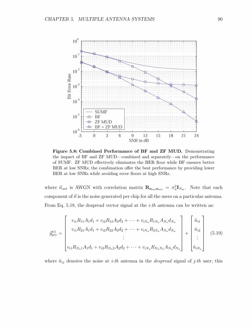
CHAPTER 5. MULTIPLE ANTENNA SYSTEMS 90
-3 0 3 6 9 12 15 18 21 2410
-6
10-5
10-4
10-3
10-2
10-1
100
SNR in dB
Bit
Err
or R
ate
SUMFBFZF MUDBF + ZF MUD
Figure 5.8: Combined Performance of BF and ZF MUD. Demonstratingthe impact of BF and ZF MUD—combined and separately—on the performanceof SUMF. ZF MUD effectively eliminates the BER floor while BF ensures betterBER at low SNRs; the combination offer the best performance by providing lowerBER at low SNRs while avoiding error floors at high SNRs.
where �nant is AWGN with correlation matrix Rnantnant = σ2nINm . Note that each
component of �n is the noise generated per chip for all the users on a particular antenna.
From Eq. 5.18, the despread vector signal at the i-th antenna can be written as:
�y(i)pre =
vi1R11A1d1 + vi2R12A2d2 + · · · + viNuR1NuANudNu
vi1R21A1d1 + vi2R22A2d2 + · · · + viNuR2NuANudNu
...
vi1RNu1A1d1 + vi2RNu2A2d2 + · · · + viNuRNuNuANudNu
+
ni1
ni2
...
niNu
(5.19)
where nij denotes the noise at i-th antenna in the despread signal of j-th user; this

CHAPTER 5. MULTIPLE ANTENNA SYSTEMS 91
noise can be represented in terms of input noise as:
nij =
∫symbolperiod
Kjn(i)ant =
N∑m=1
cjmn(i)m (5.20)
where cjm denotes the m-th chip value of the j-th user, and nim denotes the input
noise generated in the m-th chip received at the i-th antenna. Noting that the noise
generated in different chips are uncorrelated, we get:
Rnij nkl= σ2
nδikRjl (5.21)
which indicates that the noise embedded in the despread signal of a user at one
antenna is uncorrelated with the noise embedded in the despread signal of any other
user at any other antenna.
After ZF decorrelation, MAI is effectively eliminated and additive noise is the only
unwanted signal for a particular user at each antenna. Let uij be the unwanted signal
for i-th user at the output of ZF filter at the j-th antenna, then:
uij =⟨i-th row of R−1, �nj
T⟩
(5.22)
which clearly indicates that:
Ruijuik= 0, ∀j �= k (5.23)
Thus the unwanted signals for the i-th beamformer are spatially uncorrelated.
Had a decorrelating filter not been used at each antenna, spatial correlation would
have existed for undesired signals at the input of each beamformer because of MAI
that is correlated with itself over the antennas. Since the decorrelating filter removes
MAI completely irrespective of the sector size, the unwanted signals into a particular
beamformer must consist of additive gaussian noise only.

CHAPTER 5. MULTIPLE ANTENNA SYSTEMS 92
-9 -6 -3 0 3 6 9 12 15 18 2110
-6
10-5
10-4
10-3
10-2
10-1
100
SNR in dB
Bit
Err
or R
ate
ZF MUD + VDBF + VDBF + ZF MUD + VD
Figure 5.9: Performance Comparison: BF + ZF MUD + VD. Comparingthe performance of Beamformer and ZF MUD combined with VD.
5.5.2 The Received Signal
We have shown that performing the R−1 decorrelation operation at each antenna
causes the undesired signal to appear as spatially white at the input of the beamformer
regardless of the sector’s angular size. Under these conditions, max-SINR algorithm
reduces to the delay-and-sum algorithm [88] which is used to generate the plots in
Fig. 5.8 and Fig. 5.9.
The received vector signal, from Eq. 5.10, can be represented as:
�r =
v11K1A1d1 + v12K2A2d2 + · · · + v1NuKNuANudNu
v21K1A1d1 + v22K2A2d2 + · · · + v2NuKNuANudNu
...
vNm1K1A1d1 + vNm2K2A2d2 + · · · + vNmNuKNuANudNu
+ �nant (5.24)
After despreading at each antenna with K1, K2, · · · , KNu , the pre-MUD signal at

CHAPTER 5. MULTIPLE ANTENNA SYSTEMS 93
the first antenna is given by:
�y(1)pre =
v11R11A1d1 + v12R12A2d2 + · · · + v1NuR1NuANudNu
v11R21A1d1 + v12R22A2d2 + · · · + v1NuR2NuANudNu
...
v11RNu1A1d1 + v12RNu2A2d2 + · · · + v1NuRNuNuANudNu
+ �n1 (5.25)
which, for the m-th user, can be written as:
�y(m)pre = R diag(vmi; 1 ≤ i ≤ Nu)A�d + �nm (5.26)
Thus by using R−1 filter, the decorrelation operation can be performed at each
antenna individually. Once the decorrelation is performed at each antenna, the sig-
nals corresponding to individual users are routed to their respective beamformers, as
indicated in Fig. 5.7.
5.6 Performance Results
Figure 5.8 compares all the schemes discussed in this chapter without any channel
encoding. It clearly indicates that for BER specifications for voice and data trans-
mission (i.e., 10−3 and 10−6 respectively), ZF MUD combined with BF outperforms
the other receivers.
Results with channel encoding are shown in Fig. 5.9. In this case, beamforming
appears to perform significantly better than multiuser detection prior to reaching a
BER floor of about 10−5. These results, however, are obtained for equal power users,
while a realistic comparison of BF and ZF MUD requires consideration of a scenario
in which users transmit unequal powers. Near-far resistance of a detector is a direct
indication of how well that detector can handle the users transmitting unequal powers.
Simulations results for BER of a far user with low SNR are shown in Fig. 5.10. These
results indicate that linear MUDs are extremely near-far resistant while BF is not.

CHAPTER 5. MULTIPLE ANTENNA SYSTEMS 94
0 2 4 6 8 10 1210
-3
10-2
10-1
100
Average Excess SNR of Strong Users [dB]
Bit
Err
or R
ate
SUMFBF (4 Antennas)ZF MUDMMSE MUDBF + ZF MUD
Figure 5.10: Near-Far Resistance. Depicting the Near-Far Resistance of var-ious receivers with 15 active users. The plot shows the BER of a far user whoseSNR is kept at 12 dB. SNR of all other users is increased progressively as indicatedon the x-axis.
On the other hand, BF is robust against unknown MAI while MUDs are not. Thus
a combination offers the best performance. For voice applications requiring BER of
10−3 or lower, the gain of ZF MUD+BF is approximately 8 dB more than a single-
antenna ZF MUD (see Fig. 5.8). A comparison of Fig. 5.8 with Fig. 5.9 indicates that
with channel encoding, an additional gain of 9 dB is obtained.

Chapter 6
Summary and Conclusions
The capacity of practical DS-CDMA systems is normally limited by the allowable
level of multiple access interference (MAI). The MAI problem is more severe in the
uplink where the transmissions originate from spatially distributed handsets than in
the downlink where transmissions originate from a single point—the base station. In
a DS-CDMA downlink, the transmitted signal is the sum of signals intended for all
users. Thus, for each user, the desired and interfering signals all follow the same
propagation path.
This thesis explores the use of detection techniques to mitigate the effects of the
uplink MAI. These techniques reduce the BER for the individual users in addition
to improving the overall system capacity. Specifically, two broad classes of multiuser
detection techniques were studied. These classes are differentiated by the use of:
i) Linear filtering.
ii) Multiple antennas.
Both these techniques have improved performance compared with the single user,
single antenna detector. But there are certain regions of SNR where the individual
techniques, i) and ii) above, suffer some performance deterioration while the combi-
nation of the two yields remarkable improvements in BER and an increase in system
capacity.
95

CHAPTER 6. SUMMARY AND CONCLUSIONS 96
Systems using linear filters for multiuser detection result in effective elimination
of MAI. Thus, a BER floor is avoided rendering the system near-far resistant. For
low SNRs, however, the linear filter suffers from poor BER characteristics. For a
practical system, which is usually set up in a near-far environment, the use of a linear
filter results in a significant improvement in BER for medium to high SNRs.
Beamforming (BF)using multiple receiving antennas reduces the BER of a user by
suppressing the signals from other users without eliminating them completely. Since
the interfering signals can not be completely removed, there exists an error floor
for the BER performance of these systems. This error floor, however, is lower than
that exhibited by a single antenna system. The use of multiple receiving antennas
generally yields better performance at low SNRs and moderate performance at high
SNRs.
Linear MUD attempts to eliminate the local-cell MAI. In contrast, a system using
multiple receiving antennas is more robust against unknown MAI that originates from
other cells. Thus, a combination of BF and linear filter is near-far resistant with
improved performance at high as well as at low SNRs.
Linear MUD uses a linear filter at the base station. Implementation of such
filtering is simplified when the signals are synchronous at the symbol level. For an
asynchronous systems, however, linear MUD is far too complex to implement. The
sub-symbol scheme, discussed in this thesis, simplifies implementation of the linear
MUD in an asynchronous system.
For completely asynchronous systems, the use of sub-symbol based linear MUD
results in a significant reduction in the BER without any decrease in the system
capacity. Furthermore, when applied to a QS-CDMA system, this MUD results in a
remarkable increase in the capacity of the system.
6.1 Contributions to Knowledge
The following are the principal contributions of the research presented in this thesis:

CHAPTER 6. SUMMARY AND CONCLUSIONS 97
i) Proposal for a novel multiuser detector using sub-symbols. This approach offers
simplified implementation and is based on dividing the symbols into segments
called sub-symbols.
ii) Proposal for diversity combining algorithms for the sub-symbol scheme. Di-
versity is achieved by virtue of the fact that each constituent sub-symbol of a
particular symbol contains the same user data.
iii) Demonstration by simulation that the bit error rates of condition number based
combining algorithms outperform all the other combining algorithms.
iv) Rules for maximizing the number of users in the sub-symbol scheme using proper
thresholds. The rules are defined in terms of the chip threshold, the condition
number threshold, and the rank threshold.
v) Discovery that use of a single sub-symbol is sufficient to outperform the con-
ventional detector in the sub-symbol scheme for large number of users in a
moderately synchronous QS-CDMA system.
vi) Demonstration that the performance difference between ZF MUD and MMSE
MUD for a synchronous CDMA system depends on the condition number of the
correlation matrices of spreading sequences. This performance disparity leads to
the invention of condition number based algorithms for sub-symbol combining.
vii) Approach to combine linear multiuser detectors with multiple antennas resulting
in improved BER performance at all SNRs. This involves performing linear
multiuser detection at each antenna and combining the outputs from these
antennas.
The first five contributions in the above list were addressed in Chapter 4, and the
last one is detailed in Chapter 5. The contribution regarding performance disparity
of ZF MUD and MMSE MUD is explained in Chapter 3.
CHAPTER 6. SUMMARY AND CONCLUSIONS 98
6.2 Future Directions
During the development of this thesis, a number of promising research avenues were
discovered. Some of them are as below.
i) RAKE combining using sub-symbols. As explained in Sec. 4.2.3, the sub-symbol
receiver reduces to a RAKE receiver when the inverse filters are eliminated. Yet,
more information on demodulated signals is available in a sub-symbol scheme
than in a RAKE receiver. While the RAKE receiver provides the correlation
product for the full symbol, partial products are available when the sub-symbol
scheme is employed. Availability of additional information in the sub-symbol
case may be explored to obtain levels of performance better than those shown
by standard RAKE receivers.
ii) Optimal algorithm for sub-symbol combining. While the “simple” combining
algorithms treat all sub-symbols in the same way, condition number based algo-
rithms weigh the sub-symbols before combining. The latter are improvements
over simple algorithms but their optimality is not proved. Obtaining an opti-
mal algorithm for sub-symbol combining is an important and interesting future
research area.
iii) Combining only “clean” sub-symbols. Inversion of correlation matrix in a sub-
symbol period results in a set of sub-symbols, some of which are clean. Sim-
ulation results presented in this thesis considered combining all sub-symbols,
whether clean or not. An algorithm that considers only clean sub-symbols is
expected to provide better performance and is also an interesting research area.
iv) Code acquisition based on linear MUD. The use of MUDs results in lower BERs.
Thus, the data signal actually transmitted can be constructed at the receiver
with higher probability which may help in solving the code acquisition problem.
v) Consideration of synchronization errors. Our simulations, which use the param-
eters recommended by WCDMA proposals, also assume ideal synchronization.

CHAPTER 6. SUMMARY AND CONCLUSIONS 99
These assumptions allowed us to use a single sample per chip for the simu-
lations. Use of multiple samples per chip is expected to be more robust when
timing and synchronization errors are present, especially in a fast fading system.
These considerations also indicate an area that can be researched further.
vi) Different methods of modulation. Results in this thesis are based on the use
of BPSK modulation. While these results are applicable to QPSK and QAM
modulation schemes, consideration of effects of other modulation methods such
as differential modulation and continuous phase modulation is an important
area that can be explored in future.

Appendix A
MMSE Linear MUD Derivation
We show that the linear filter for MMSE MUD is given by:
WMMSE =(R + σ2
nA−2)−1
(A.1)
where R is the correlation matrix of the spreading sequences, A is a diagonal matrix
containing Rayleigh fading amplitudes for all users and σ2n is the input noise variance
per sample. From Eq. 3.9, the signal at the output of SUMFs is:
�y = RA�d + �n (A.2)
Let �x be the faded data signal defined as �x = A�d, and W is the linear filter through
which the SUMF output �y is processed. The MMSE filter WMMSE, by definition,
minimizes the mean squared value of the difference signal �x − W�y and is given by:
WMMSE = arg minW
E [(�x − W�y)(�x − W�y)∗] (A.3)
where * in the superscript denotes conjugate transpose. Solving, we get [95]:
WMMSE = RxyR−1yy (A.4)
100

APPENDIX A. MMSE LINEAR MUD DERIVATION 101
where Rxy is the cross-correlation matrix of �x and �y while Ryy is the autocorrelation
matrix of �y. These matrices can be evaluated as follows:
Rxy = E[�x�y∗]
= E[A�d(�d∗A∗R∗ + �n∗)]
= σ2BPSKAA∗R∗
= AA∗R (A.5)
Ryy = E[�y�y∗]
= E[(RA�d + �n)(�d∗A∗R∗ + �n∗)]
= RAA∗R + σ2nR (A.6)
Using Eq. A.5 and Eq. A.6 in Eq. A.4, the MMSE linear filter is given as:
WMMSE = AA∗R(RAA∗R + σ2nR)−1
=(R + σ2
nA−2)−1
(A.7)
The term σ2nA
−2 represents inverse SNR for a unit amplitude vector signal. Thus,
the linear filter for an MMSE multiuser detector is given by(R + 1
SNR
)−1.

Appendix B
Computation of SNR Penalty
The SNR penalty of a sub-symbol multiuser detection scheme is defined as the dif-
ference in input SNRs of the sub-symbol scheme for an asynchronous system and the
ideal ZF detector for a synchronous system when both systems exhibit the same BER.
Thus, it is also equivalent to the reduction in output SNR for a sub-symbol scheme;
this reduction is a result of reduced processing gain. In this appendix, we derive an
expression for the SNR penalty when a sub-symbol scheme is used in a DS-CDMA
system. We assume a spreading factor of N = 255 chips per symbol and a sampling
rate of one sample per chip; these values are used in all the simulations performed to
obtain the results presented in this thesis.
To characterize the SNR penalty, we compute the output SNR in two cases: ideal
full-symbol synchronous case, and the sub-symbol case. For sub-symbol case, the
“select-best” simple combining algorithm, as described in Sec. 4.3, is used. We fur-
ther assume that the fading imposes a fixed penalty for each receiver such that the
performance of any two receivers is affected by fading in the same way. This assump-
tion allows comparing non-fading systems and extending the results to those fading
systems that undergo similar kind of fading. For comparing different receivers, these
assumptions are generally valid as the receivers are used in the same environment
and the change in sampling rate has similar effects on each receiver considered.
Let S denote the total output signal and X the total output noise in the same
interval. We use subscript “f” to refer to the case of full-symbol synchronous system,
102

APPENDIX B. COMPUTATION OF SNR PENALTY 103
and subscript “s” for the case of sub-symbol synchronous receiver. For the i-th user,
the SNR for the two cases is computed as follows:
Full-symbol correlation: In this case, the decorrelation is performed over one full
symbol, such that the output signal and output noise are given by:
Sf =N∑
m=1
cimcim = N (B.1)
Xf =N∑
m=1
cimXm = ci1X1 + ci2X2 + · · · + ciNXN (B.2)
where Xm’s are i.i.d. Normal(0, σ2n) random variables that indicate the additive noise
per sample at the input of the receiver and cim is the m-th chip value in the spreading
sequence for the i-th user.
The output SNR can be computed from σ2Sf
and σ2Xf
as follows:
σ2Sf
= N2 (B.3)
σ2Xf
=N∑
m=1
cim2σ2
X1= Nσ2
n (B.4)
SNRf =σ2
Sf
σ2Xf
=N
σ2n
(B.5)
Sub-symbol correlation: Let M be the number of chips in the best sub-symbol,1
used by the select-best algorithm. Using a similar procedure as in the case of full-
symbol correlation, we can write the expressions for output signal and noise as:
Ss =M∑i=1
1 = M (B.6)
Xs = X1 + X2 + · · · + XM (B.7)
σ2Xs
= Mσ2X1
= Mσ2n (B.8)
1Best sub-symbol is the one used in select-best combining and is described as the one in whichthe sum of signal, noise, and MAI is largest. See Sec. 4.3 for details.

APPENDIX B. COMPUTATION OF SNR PENALTY 104
and the output SNR is, therefore, computed as:
σ2Ss
= M2 (B.9)
σ2Xs
=M∑
m=1
cim2σ2
X1= Mσ2
n (B.10)
SNRf =σ2
Ss
σ2Xs
=M
σ2n
(B.11)
SNR Penalty: The SNR penalty δs can be computed from expressions for SNRf
and SNRs, as follows:
δs =SNRf
SNRs
=N
M(B.12)
We may assume that M is approximately equal to the expected number of chips in the
longest sub-symbol within a symbol, the accuracy of the result mostly dependenpt on
this approximation. In a slow fading environment, this approximation is reasonably
good since the longest sub-symbol would yield the best amplitude when integrated
over its own length. We can compute M analytically. The analysis, however, becomes
cumbersome for a large number of sub-symbols. In such a case, we compute M by
simulations.
For 12 asynchronous users with uniformly distributed random transmission in-
stants, M is found to be approximately 55. SNR penalty for the select-best algo-
rithm is, therefore, approximated by 25555
= 4.64 = 6.7 dB which agrees with the
results depicted in Fig. 4.6. For condition number based accumulate combining, an
SNR penalty of 2 dB is observed from Fig. 4.7; this corresponds to the use of approxi-
mately 161 chips to perform correlation in a sub-symbol scheme employing select-best
simple combining algorithm. Thus, combining many sub-symbols, weighted by the in-
verse condition numbers of corresponding correlation matrices, results in a reduction
in SNR penalty.

Appendix C
Simulation Parameters
For the simulations, we use parameters recommended in proposed WCDMA standards
[63]. Following table summarizes the system parameters used in the simulations
presented in this thesis:
Common System Parameters
Carrier Frequency 1.9 GHz
Spreading Sequences Kasami (small set)
Spreading gain (chips per bit) 255
Sampling Rate 1 sample/chip
Modulation BPSK
Convolutional code Rate 12
Constraint Length 5
Maximum Mobile Speed 120 Km/hr
Maximum doppler 211 Hz
Environment Outdoor
Angular Spread Narrow
Number of Receive Antennas 1 (unless specified otherwise)
Fading Flat Rayleigh
Number of Users 12 (unless specified otherwise)
Table C.1: WCDMA simulation parameters.
105

Bibliography
[1] G. C. Di Piazza, A. Plitkins, and G. I. Zysman, “The Cellular Concept,” Bell
Systems Technical Journal, vol. 58, no. 1, pp. 215–48, January 1979.
[2] R. Nelson and D. Westin, “The Evolution of the North American Cellular Net-
work,” Telecommunications (International Edition), vol. 26, no. 9, pp. 24–28,
September 1992.
[3] V. H. MacDonald, “The Cellular Concept,” Bell Systems Technical Journal, vol.
58, no. 1, pp. 15–42, January 1979.
[4] F. H. Blecher, “Advanced Mobile Phone Service,” IEEE Transactions on Vehic-
ular Technology, vol. VT-29, no. 2, pp. 238–244, May 1980.
[5] E. S. K. Chien, “AT&T Cellular System-System Description and System Trial
Results,” in Proceedings of the ICC, vol. 3, pp. 1207–1213, May 1984.
[6] D. C. Cox, “A Radio System Proposal for Widespread Low Power Tetherless
Communications,” IEEE Transactions on Communications, vol. 39, no. 2, pp.
324–335, February 1991.
[7] D. L. Huff, “AT&T Cellular Technology Review,” in Proceedings of MILCOM
1985, vol. 2, pp. 490–494, October 1985.
[8] J. E. Padgett, C. G. Gunther, and T. Hattori, “Overview of Wireless Personal
Communications,” IEEE Communications Magazine, pp. 28–41, January 1995.
106
BIBLIOGRAPHY 107
[9] L. R. Maciel and H. L. Bertoni, “Cell Shape for Microcellular Systems in Resi-
dential and Commercial Environments,” IEEE Transactions on Vehicular Tech-
nology, vol. 43, no. 2, pp. 270–278, May 1994.
[10] M. Gustafsson, K. Jamal, and E. Dahlman, “Compressed Mode Techniques for
Interfrequency Measurements in a Wide-band DS-CDMA System,” in Proc. of
PIMRC ’97, pp. 23–35, Helsinki, Finland, September 1997.
[11] T. S. Rappaport, Wireless Communications: Principles and Practice, Prentice-
Hall, NJ, 1996, ISBN:0133755363.
[12] A. Andreadis, G. Benelli, G. Giambene, and B. Marzucchi, “Performance analy-
sis of the WAP protocol over GSM-SMS,” in Proceedings of the ICC, vol. 2, pp.
467–471, June 2001.
[13] W. C. Y. Lee, “Smaller Cells for Greater Performance,” IEEE Communications
Magazine, vol. 29, no. 11, pp. 19–23, November 1991.
[14] W. C. Y. Lee, “Cellular Telephone System,” U.S. Patent 4,932,049, June 1990,
Patent Assigned on June 05, 1990.
[15] M. Schwartz, Telecommunication Networks: Protocols, Modeling, and Analysis,
Addison-Wesley Pub. Co., Reading, MA, August 1986, ISBN:020116423X.
[16] D. A. Harvey and R. Santalesa, “Wireless Gets Real,” BYTE, vol. 19, no. 5, pp.
90–96, May 1994.
[17] TIA/EIA IS-54, “Cellular System Dual-Mode Mobile Station-Base Station Com-
patibility Standard,” Standard Document, April 1992, Telecommunication In-
dustry Association Standard.
[18] TIA/EIA IS-95, “Mobile Station-Base Station Compatibility Standard for Dual-
Mode Wideband Spread-Spectrum Cellular Systems,” Standard Document, July
1993, Telecommunication Industry Association Standard.

BIBLIOGRAPHY 108
[19] G. Keiser, Local Area Networks, McGraw-Hill, New York, 2nd edition, 2002,
ISBN:0072393432.
[20] N. Abramson, “Multiple Access in Wireless Digital Networks,” Proceedings of
the IEEE, vol. 82, no. 9, pp. 1360–1370, September 1994.
[21] L. Kleinrock, “On Some Principles of Nomadic Computing and Multi-Access
Communications,” IEEE Communications Magazine, pp. 46–50, July 2000.
[22] J. G. Proakis, Digital Communications, McGraw-Hill, New York, 3rd edition,
1995, ISBN:0070517266.
[23] ETSI, “GSM Specifications, Series 01-12,” Standard Document, ETSI Standard.
[24] G. Brasche and B. Walke, “Concepts, Services, and Protocols of the New GSM
Phase 2+ General Packet Radio Service,” IEEE Communications Magazine, vol.
35, no. 8, pp. 94 –104, August 1997.
[25] J. Cai and D. J. Goodman, “General Packet Radio Service in GSM,” IEEE
Communications Magazine, vol. 35, no. 10, pp. 122–131, October 1997.
[26] R. V. Nobelen, N. Seshadri, J. Whitehead, and S. Timiri, “An adaptive radio
link protocol with enhanced data rates for GSM evolution,” IEEE Personal
Communications, pp. 54–64, February 1999.
[27] B. Jabbari, “Cost-effective Networking via Digital Satellite Communications,”
Proceedings of the IEEE, vol. 72, no. 11, pp. 1556–1563, November 1984.
[28] M. Rahnema, “Overview of the GSM System and Protocol Architecture,” IEEE
Communications Magazine, vol. 31, no. 4, pp. 92–100, April 1993.
[29] W. Stallings, Data and Computer Communications, Prentice-Hall, Englewood
Cliffs, NJ, 6th edition, November 1999, ISBN:0130843709.
[30] A. S. Tanenbaum, Computer Networks, Prentice-Hall, Englewood Cliffs, NJ, 3rd
edition, January 1996, ISBN:0133499456.

BIBLIOGRAPHY 109
[31] C. A. Sunshine, Computer Network Architectures and Protocols, Plenum Pub-
lishing Corp, New York, 2nd edition, October 1989, ISBN:0306431890.
[32] D. V. Sarwate and M. B. Pursley, “Crosscorrelation Properties of Pseudorandom
and Related Sequences,” Proceedings of the IEEE, vol. 68, no. 5, pp. 593–619,
May 1980.
[33] R. Prasad, CDMA for Wireless Personal Communications, Artech House, Nor-
wood, MA, 1996, ISBN:0890065713.
[34] M. K. Simon, J. K. Omura, R. A. Scholtz, and B. K. Levitt, Spread Spectrum
Communications, Computer Science Press, MD, 1985, ISBN:0881750174.
[35] E. H. Dinan and B. Jabbari, “Spreading Codes for Direct Sequence CDMA and
Wideband CDMA Cellular Networks,” IEEE Communications Magazine, pp.
48–54, September 1998.
[36] S. Verdu, Multiuser Detection, Cambridge University Press, Cambridge, UK,
1998, ISBN:0521593735.
[37] S. Moshavi, “Multi-User Detection for DS-CDMA Communications,” IEEE
Communications Magazine, pp. 124–136, October 1996.
[38] A. Duel-Hallen, J. Holtzman, and Z. Zvonar, “Multiuser Detection for CDMA
Systems,” IEEE Personal Communications, pp. 46–58, April 1995.
[39] E. S. Esteves and R. A. Scholtz, “Bit Error Probability of Linear Multiuser De-
tectors in the Presence of Unknown Multiple Access Interference,” in Proceedings
of the IEEE Globecom, vol. 2, pp. 599–603, November 1997.
[40] M. K. Simon, J. K. Omura, R. A. Scholtz, and B. K. Levitt, Spread Spectrum
Communications Handbook, McGraw-Hill, New York, 1994, ISBN:0071369643.
[41] B. P. Lathi, Modern Digital and Analog Communications Systems, McGraw-Hill,
New York, 2001, ISBN:0070111278.

BIBLIOGRAPHY 110
[42] A. B. Carlson, P. B. Crilly, and J. C. Rutledge, Communication systems: An In-
troduction to Signals and Noise in Electrical Communication, Oxford University
Press, New York, 1998, ISBN:0195110099.
[43] A. J. Goldsmith, Course Reader: Advanced Topics in Wireless Communications,
Stanford University, Stanford, CA, Spring 1999.
[44] D. C. Cox, “910 MHz urban mobile radio propagation: Multipath characteristics
in New York City,” IEEE Transactions on Communications, vol. COM-21, no.
11, pp. 1188–1194, November 1973.
[45] W. C. Jakes, Microwave Mobile Communications, Wiley, New York, 1974,
ISBN:0780310691.
[46] G. L. Stuber, Principles of Mobile Communication, Kluwer Academic Publishers,
MA, 2nd edition, February 2001, ISBN:0792379985.
[47] S. Ramo, J. R. Whinnery, and T. Van Duzer, Fields and Waves in Communica-
tion Electronics, John Wiley & Sons, New York, 1993, ISBN:0471585513.
[48] N. Amitay, “Modeling and Computer Simulation of Wave Propagation in Lineal
Line-of-sight Microcells,” IEEE Transactions on Vehicular Technology, vol. VT-
41, no. 4, pp. 337–342, November 1992.
[49] J. W. McKown and R. L. Hamilton, “Ray Tracing as a Design Tool for Radio
Networks,” IEEE Network, vol. 5, no. 6, pp. 27–30, November 1991.
[50] K. Schaubach, N. J. Davis IV, and T. S. Rappaport, “A Ray Tracing Method for
predicting path loss and delay spread in microcellular environment,” in IEEE
Vehicular Technology Conference Records, pp. 932–935, May 1992.
[51] M. C. Lawton and J. P. McGeehan, “The application of GTD and ray launching
techniques to channel modelling for cordless radio systems,” in IEEE Vehicular
Technology Conference Records, pp. 125–130, May 1992.
BIBLIOGRAPHY 111
[52] F. Niu and H. L. Bertoni, “Path Loss and Cell Coverage of Urban Microcells in
High-Rise Building Environments,” in Proceedings of the IEEE Globecom, vol. 1,
pp. 266–270, November 1993.
[53] M. D. Yacoub, Foundations of Mobile Radio Engineering, CRC Press, Boca
Raton, FL, 1993, ISBN:0849386772.
[54] H. L. Bertoni, W. Honcharenko, L. R. Maciel, and H. H. Xia, “UHF Propagation
Prediction for Wireless Personal Communications,” Proceedings of the IEEE, vol.
82, no. 9, pp. 1333–1359, September 1994.
[55] S. Ross, A First Course in Probability, Prentice-Hall, New York, 6th edition,
2001, ISBN:0130338516.
[56] F. Ikegami, S. Takeuchi, and S. Yoshida, “Theoretical prediction of mean field
strength for urban mobile radio,” IEEE Transactions on Antennas and Propa-
gation, vol. AP-39, no. 3, pp. 299–302, March 1991.
[57] M. Hata, “Empiricla formula for propagation loss in land mobile radio services,”
IEEE Transactions on Vehicular Technology, vol. VT-29, no. 3, pp. 317–325,
August 1980.
[58] M. Gudmundson, “Correlation Model for Shadow Fading in Mobile Radio Sys-
tems,” Electronics Letters, vol. 27, no. 23, pp. 2145–2146, November 1991.
[59] R. S. Kennedy, Fading Dispersive Communication Channels, Wiley, New York,
1969, ISBN:0471469033.
[60] S. O. Rice, “Mathematical Analysis of Random Noise-I,” Bell Systems Technical
Journal, vol. 23, no. 7, pp. 282–333, July 1944.
[61] S. O. Rice, “Mathematical Analysis of Random Noise-II,” Bell Systems Technical
Journal, vol. 24, no. 1, pp. 46–156, January 1945.

BIBLIOGRAPHY 112
[62] S. Glisic and B. Vucetic, Spread Spectrum CDMA Systems for Wireless Com-
munications, Artech House, Norwood, MA, 1997, ISBN:0890068585.
[63] Evaluation Document Concept Group Alpha-WCDMA, “Part-1: System De-
scription; Performance Evaluation,” Tdoc SMG 905/97.
[64] H. F. A. Roefs, Binary Sequences for Spread-Spectrum Multiple-Access Commu-
nications, Ph.D. thesis, University of Illinois, Urbana, Illinois, 1997.
[65] R. Gold, “Optimal Binary Sequences for Spread Spectrum Multiplexing,” IEEE
Transactions on Information Theory, vol. IT-13, pp. 619–621, October 1967.
[66] J. H. Lindholm, “An Analysis of the Pseudo-Randomness Properties of Subse-
quences of Long m-Sequnces,” IEEE Transactions on Information Theory, vol.
IT-14, pp. 569–576, July 1968.
[67] R. Gold, “Maximal Recursive Sequences with 3-valued Recursive Cross-
correlation Functions,” IEEE Transactions on Information Theory, vol. IT-14,
pp. 154–156, January 1968.
[68] A. Leon-Garcia, Probability and Random Processes for Electrical Engineering,
Addison-Wesley, Reading, MA, 2nd edition, 1994, ISBN:020150037X.
[69] V. Heeswyk, “A Delay Independent Decorrelating Detector for Quasi-
Synchronous CDMA,” IEEE Journal on Selected Areas in Communications,
vol. 14, no. 8, pp. 1619–1626, October 1996.
[70] Z. A. Uzmi and M. J. Narasimha, “Maximizing System Capacity in a Sub-symbol
Based DS-CDMA Multiuser Detector,” in Proceedings of the IEEE Globecom,
vol. 1, pp. 15–19, November 2000.
[71] G. L. Turin, “The Effects of Multipath and Fading on the Performance of Direct-
Sequence CDMA Systems,” IEEE JSAC, vol. SAC-2, no. 4, pp. 597–603, July
1984.

BIBLIOGRAPHY 113
[72] M. K. Simon and M.-S. Alouini, “A unified approach to the performance analysis
of digital communication over generalized fading channels,” Proceedings of the
IEEE, vol. 86, no. 9, pp. 1860–1877, September 1998.
[73] M.-S. Alouini, M. K. Simon, and A. Goldsmith, “A unified performance analysis
of DS-CDMA systems over generalized frequency-selective fading channels,” in
IEEE International Symposium on Information Theory, pp. 16–21, August 1998.
[74] M.-S. Alouini and M. K. Simon, “An MGF-based performance analysis of gen-
eralized selection combining over Rayleigh fading channels,” IEEE Transactions
on Communications, vol. 48, no. 3, pp. 401 –415, March 2000.
[75] M.-S. Alouini and M. K. Simon, “Performance of coherent receivers with hybrid
SC/MRC over Nakagami-m fading channels,” IEEE Transactions on Vehicular
Technology, vol. 48, no. 4, pp. 1155–1164, July 1999.
[76] R. Lupas and S. Verdu, “Linear Multiuser Detectors for Synchronous Code-
division Multiple-Access Channels,” IEEE Trans. Info. Theory, vol. 35, no. 1,
pp. 123–136, January 1989.
[77] H. V. Poor and S. Verdu, “Probability of Error in Multiuser Detection,” IEEE
Trans. Info. Theory, vol. 43, no. 3, pp. 858–871, May 1997.
[78] Z. A. Uzmi and S. A. Mujtaba, “A Novel Scheme for Linear Multiuser Detec-
tion in Asynchronous DS-CDMA Systems with Frequency Selective Fading,” in
Proceedings of the IEEE Globecom, vol. 1b, pp. 981–985, December 1999.
[79] S. Verdu, “Minimum Probability of Error for Asynchronous Gaussian Multiple-
Access Channels,” IEEE Transactions on Information Theory, vol. IT-32, no. 1,
pp. 85–96, January 1986.
[80] R. Lupas and S. Verdu, “Near-Far Resistance of Multiuser Detectors in Asyn-
chronous Channels,” IEEE Transactions on Communications, vol. 38, no. 4, pp.
496–508, April 1990.

BIBLIOGRAPHY 114
[81] Fu-Chun Zheng and S. K. Barton, “Near-Far Resistant Detection of CDMA
Signals via Isolation Bit Insertion,” IEEE Transactions on Communications,
vol. 43, no. 2/3/4, pp. 1313–1317, Feb/Mar/Apr 1995.
[82] Z. Zvonar and D. Brady, “Suboptimal Multiuser Detector for Frequency-Selective
Rayleigh Fading Synchronous CDMA Channels,” IEEE Transactions on Com-
munications, vol. 43, no. 2/3/4, pp. 154–157, Feb/Mar/Apr 1995.
[83] H. C. Huang and S. Verdu, “Linear Differentially Coherent Multiuser Detection
for Multipath Channels,” Wireless Personal Communications, vol. 6, no. 1-2,
pp. 113–136, January 1998.
[84] Qualcomm. Inc., “Wideband Spread Spectrum Digital Cellular System,” Pro-
posed EIA/TIA Interim Standard, April 1992.
[85] J. H. Winters, “Smart Antennas for Wireless Communications,” IEEE Personal
Communications, pp. 36–48, February 1998.
[86] M. C. Vanderveen, Estimation of Parametric Channel Models in Wireless Com-
munication Networks, Ph.D. thesis, Stanford University, Stanford, CA, 1998.
[87] L. C. Godara, “Application of Antenna Arrays to Mobile Communications, Part
II: Beam-Forming and Direction-of-Arrival Considerations,” Proceedings of the
IEEE, vol. 85, no. 8, pp. 1195–1245, August 1997.
[88] A. F. Naguib, Adaptive Antennas for CDMA Wireless Networks, Ph.D. thesis,
Stanford University, Stanford, CA, 1996.
[89] D. H. Johnson and D. E. Dudgeon, Array Signal Processing: Concepts and
Techniques, Prentice-Hall, Englewood Cliffs, NJ, 1993, ISBN:0130485136.
[90] V. Tarokh, N. Seshadri, and A. R. Calderbank, “Space-Time Codes for High Data
Rate Wireless Communication: Performance Criterion and Code Construction,”
IEEE Transactions on Information Theory, vol. 44, no. 2, pp. 744–765, March
1998.

BIBLIOGRAPHY 115
[91] A. Wittneben, “A New Bandwidth Efficient Transmit Antenna Modulation Di-
versity Scheme for Linear Digital Modulation,” in Proceedings of the ICC, pp.
1630–1634, 1993.
[92] V. Tarokh, A. Naguib, N. Seshadri, and A. R. Calderbank, “Combined Array
Processing and Space-Time Coding,” IEEE Transactions on Information Theory,
vol. 45, no. 4, pp. 1121–1128, May 1999.
[93] J. Choi, “Beamforming for the Multiuser Detector in Synchronous CDMA Sys-
tems: Approaches and Performance Analysis,” Signal Processing, Elsevier for
EURASIP, vol. 60, no. 2, pp. 195–211, July 1997.
[94] Z. Zvonar, “Beamforming for the Multiuser Detector in Synchronous CDMA Sys-
tems: Approaches and Performance Analysis,” IEEE Transactions on Vehicular
Technology, vol. 45, no. 1, pp. 205–211, February 1996.
[95] T. Kailath, A. H. Sayed, and B. Hassibi, Linear Estimation, Prentice-Hall,
Upper Saddle River, NJ, 2000, ISBN:0130224642.


![Nonlinear Multi-Antenna Detection Methods · multiuser detection designed for code-division multiple-access (CDMA) [16]–[20]. In fact, it has been observed even in linearly separable](https://img.dokumen.tips/doc/110x75/603db2432ffb6326e07b3a30/nonlinear-multi-antenna-detection-methods-multiuser-detection-designed-for-code-division.jpg)