Semiparametric modeling of autonomous nonlinear dynamical

systems with applications

Debashis Paul∗, Jie Peng∗ & Prabir Burman

Department of Statistics, University of California, Davis

Abstract

In this paper, we propose a semi-parametric model for autonomous nonlinear dynamicalsystems and devise an estimation procedure for model fitting. This model incorporates subject-specific effects and can be viewed as a nonlinear semi-parametric mixed effects model. Wealso propose a computationally efficient model selection procedure. We prove consistency of theproposed estimator under suitable regularity conditions. We show by simulation studies that theproposed estimation as well as model selection procedures can efficiently handle sparse and noisymeasurements. Finally, we apply the proposed method to a plant growth data used to studygrowth displacement rates within meristems of maize roots under two different experimentalconditions.

Key words: autonomous dynamical systems; nonlinear optimization; Levenberg-Marquardtmethod; leave-one-curve-out cross-validation; plant growth

1 Introduction

Continuous time dynamical systems arise, among other places, in modeling certain biological pro-cesses. For example, in plant science, the spatial distribution of growth is an active area of research(Basu et al., 2007; Schurr, Walter and Rascher, 2006; van der Weele et al., 2003; Walter et al.,2002). One particular region of interest is the root apex, which is characterized by cell division,rapid cell expansion and cell differentiation. A single cell can be followed over time, and thus itis relatively easy to measure its cell division rate. However, in a meristem1, there is a changingpopulation of dividing cells. Thus the cell division rate, which is defined as the local rate of forma-tion of cells, is not directly observable. If one observes root development from an origin attachedto the apex, tissue elements appear to flow through, giving an analogy between primary growthin plant root and fluid flow (Silk, 1994). Thus in Sacks, Silk and Burman (1997), the authorspropose to estimate the cell division rates by a continuity equation that is based on the principleof conservation of mass. Specifically, if we assume a steady growth, then the cell division rateis estimated as the gradient (with respect to distance) of cell flux – the rate at which cells aremoving past a spatial point. Cell flux is the product of cell number density and growth velocityfield. The former can be found by counting the number of cells per small unit file. The latter is

∗equal contributors1meristem is the tissue in plants consisting of undifferentiated cells and found in zones of the plant where growth

can take place.

1

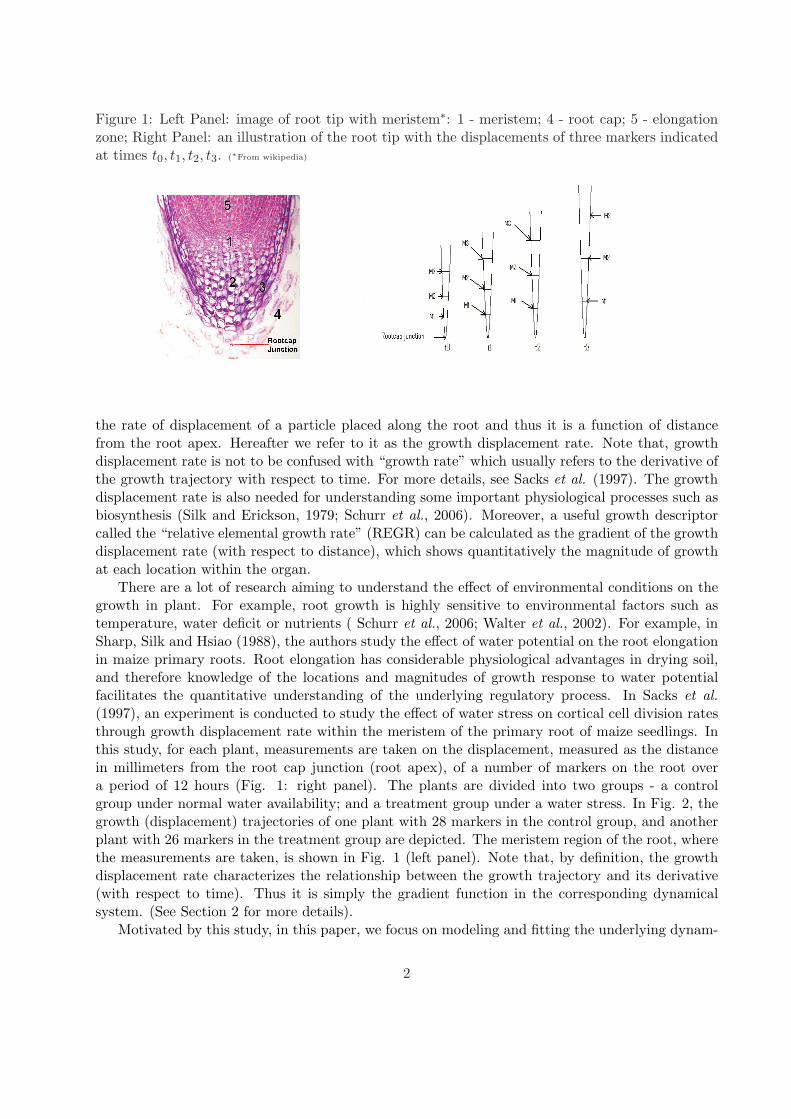
Figure 1: Left Panel: image of root tip with meristem∗: 1 - meristem; 4 - root cap; 5 - elongationzone; Right Panel: an illustration of the root tip with the displacements of three markers indicatedat times t0, t1, t2, t3. (∗From wikipedia)

the rate of displacement of a particle placed along the root and thus it is a function of distancefrom the root apex. Hereafter we refer to it as the growth displacement rate. Note that, growthdisplacement rate is not to be confused with “growth rate” which usually refers to the derivative ofthe growth trajectory with respect to time. For more details, see Sacks et al. (1997). The growthdisplacement rate is also needed for understanding some important physiological processes such asbiosynthesis (Silk and Erickson, 1979; Schurr et al., 2006). Moreover, a useful growth descriptorcalled the “relative elemental growth rate” (REGR) can be calculated as the gradient of the growthdisplacement rate (with respect to distance), which shows quantitatively the magnitude of growthat each location within the organ.

There are a lot of research aiming to understand the effect of environmental conditions on thegrowth in plant. For example, root growth is highly sensitive to environmental factors such astemperature, water deficit or nutrients ( Schurr et al., 2006; Walter et al., 2002). For example, inSharp, Silk and Hsiao (1988), the authors study the effect of water potential on the root elongationin maize primary roots. Root elongation has considerable physiological advantages in drying soil,and therefore knowledge of the locations and magnitudes of growth response to water potentialfacilitates the quantitative understanding of the underlying regulatory process. In Sacks et al.(1997), an experiment is conducted to study the effect of water stress on cortical cell division ratesthrough growth displacement rate within the meristem of the primary root of maize seedlings. Inthis study, for each plant, measurements are taken on the displacement, measured as the distancein millimeters from the root cap junction (root apex), of a number of markers on the root overa period of 12 hours (Fig. 1: right panel). The plants are divided into two groups - a controlgroup under normal water availability; and a treatment group under a water stress. In Fig. 2, thegrowth (displacement) trajectories of one plant with 28 markers in the control group, and anotherplant with 26 markers in the treatment group are depicted. The meristem region of the root, wherethe measurements are taken, is shown in Fig. 1 (left panel). Note that, by definition, the growthdisplacement rate characterizes the relationship between the growth trajectory and its derivative(with respect to time). Thus it is simply the gradient function in the corresponding dynamicalsystem. (See Section 2 for more details).

Motivated by this study, in this paper, we focus on modeling and fitting the underlying dynam-

2

Figure 2: Growth trajectories for plant data. Left panel : a plant in control group; Right panel :a plant in treatment group

0 2 4 6 8

02

46

81

01

2

time (in hrs)

dis

tan

ce f

rom

ro

ot

cap

ju

ncti

on

(in

mm

)

control group

0 2 4 6 80

24

68

time (in hrs)

dis

tan

ce f

rom

ro

ot

cap

ju

ncti

on

(in

mm

)

treatment group

ical system based on data measured over time (referred as sample curves or sample paths) for agroup of subjects. In particular, we are interested in the case where there are multiple replicatescorresponding to different initial conditions for each subject. Moreover, for a given initial condition,instead of observing the whole sample path, measurements are taken only at a sparse set of timepoints together with (possible) measurement noise. In the plant data application, each plant is asubject. And the positions of the markers which are located at different distances at time zero fromthe root cap junction correspond to different initial conditions. There are in total 19 plants and 445sample curves in this study. The number of replicates (i.e. markers) for each plant varies between10 and 31. Moreover, smoothness of the growth trajectories indicates low observational noise levelsand an absence of extraneous shocks in the system. Hence, in this paper, we model the growthtrajectories through deterministic differential equations with plant-specific effects. We refer to the(common) gradient function of these differential equations as the baseline growth displacement rate.

We first give a brief overview of the existing literature on fitting smooth dynamical systems incontinuous time. A large number of physical, chemical or biological processes are modeled throughsystems of parametric differential equations (cf. Ljung and Glad, 1994, Perthame, 2007, Strogatz,2001). Ramsay, Hooker, Campbell and Cao (2007) consider modeling a continuously stirred tankreactor. Zhu and Wu (2007) adopt a state space approach for estimating the dynamics of cell-virusinteractions in an AIDS clinical trial. Poyton et al. (2006) use the principal differential analysisapproach to fit dynamical systems. Recently Chen and Wu (2008a, 2008b) propose to estimatedifferential equations with known functional forms and nonparametric time-dependent coefficients.Wu and Ding (1999) and Wu, Ding and DeGruttola (1998) propose using nonlinear least squaresprocedure for fitting differential equations that take into account subject-specific effects. In a recentwork, Cao, Fussmann and Ramsay (2008) model a nonlinear dynamical system using splines withpredetermined knots for describing the gradient function. Most of the existing approaches assume

3

known functional forms of the dynamical system; and many of them require data measured on adense grid (e.g., Varah, 1982; Zhu and Wu, 2007).

For the problems that we are interested in this paper, measurements are taken on a sparse setof points for each sample curve. Thus numerical procedures for solving differential equations canbecome unstable if we treat each sample curve separately. Moreover, we are more interested inestimating the baseline dynamics than the individual dynamics of each subject. For example, inthe plant study described above, we are interested in comparing the growth displacement rates(as a function of distance from the root cap junction) under two different experimental conditions.On the other hand, we are not so interested in the displacement rate corresponding to each plant.Another important aspect in modeling data with multiple subjects is that adequate measures needto be taken to model possible subject-specific effects, otherwise the estimates of model parameterscan have inflated variability. Thus in this paper, we incorporate subject-specific effects into themodel while combining information across different subjects. In addition, because of insufficientknowledge of the problem as is the case for the plant growth study, in practice one often has to resortto modeling the dynamical system nonparametrically. For example, there is controversy amongplant scientists about whether there is a growth bump in the middle of the meristem. There arealso some natural boundary constraints of the growth displacement rate, making it hard to specifya simple and interpretable parametric system. (See more discussions in Section 3). Therefore,in this paper, we propose to model the baseline dynamics nonparametrrically through a basisrepresentation approach. We use an estimation procedure that combines nonlinear optimizationtechniques with a numerical ODE solver to estimate the unknown parameters. In addition, we derivea computationally efficient approximation of the leave-one-curve-out cross validation score for modelselection. We prove consistency of the proposed estimators under appropriate regularity conditions.Our asymptotic scenario involves keeping the number of subjects fixed and allowing the number ofmeasurements per subject to grow to infinity. The analysis differs from the usual nonparametricregression problems due to the structures imposed by the differential equations model. We showby simulation studies that the proposed approach can efficiently estimate the baseline dynamicsunder the setting of multiple replicates per subject with sparse noisy measurements. Moreover,the proposed model selection procedure is effective in maintaining a balance between fidelity tothe data and to the underlying model. Finally, we apply the proposed method to the plant datadescribed earlier and compare the estimated growth displacement rates under the two experimentalconditions.

The rest of paper is organized as follows. In Section 2, we describe the proposed model. InSections 3 and 4, we discuss the model fitting and model selection procedures, respectively. InSection 5, we prove consistency of the proposed estimator. In Section 6, we conduct simulationstudies to illustrate finite sample performance of the proposed method. Section 7 is the applicationof this method to the plant data. Technical details are in the appendices. An R package dynamicsfor fitting the model described in this paper is available upon request.

2 Model

In this section, we describe a class of autonomous dynamical systems that is suitable for modelingthe problems exemplified by the plant data (Section 1). An autonomous dynamical system has thefollowing general form:

X ′(t) = f(X(t)), t ∈ [T0, T1].

4

Figure 3: Empirical derivatives (divided differences) X ′(t) against empirical fits (averaged mea-surements) X(t) for treatment group.

0 2 4 6 8 10

−1.0

−0.5

0.0

0.5

1.0

1.5

2.0

2.5

X(t) (in mm)

X’(t)

(in

mm

/hr)

Without loss of generality, henceforth T0 = 0 and T1 = 1. Note that, the above equation meansthat X(t) = a +

∫ t0 f(X(u))du, where a = X(0) is the initial condition. Thus in an autonomous

system, the dynamics (which is characterized by f) depends on time t only through X(t). Thistype of systems arises in various scientific studies such as modelling prey-predator dynamics, virusdynamics, or epidemiology (cf. Perthame, 2007). Many studies in plant science such as Silk (1994),Sacks et al. (1997), Fraser, Silk and Rost (1990) all suggest reasonably steady growth velocityacross the meristem under both normal and water-stress conditions at an early developmentalstage. Moreover, exploratory regression analysis based on empirical derivatives and empirical fitsof the growth trajectories indicates that time is not a significant predictor and thus an autonomousmodel is reasonable. This assumption is equivalent to the assertion that the growth displacementrate depends only on the distance from the root cap junction. It means that time zero does notplay a role in terms of estimating the dynamical system and there is also no additional variationassociated with individual markers.

Figure 3 shows the scatter plot of empirical derivatives versus empirical fits in the treatmentgroup. It indicates that there is an increase in the growth displacement rate starting from a zerorate at the root cap junction, then followed by a nearly constant rate beyond a certain location.This means that growth stops beyond this point and the observed displacements are due to growthin the part of the meristem closer to the root cap junction. Where and how growth stops is ofgreat scientific interest. The scatter plot also indicates excess variability towards the end which isprobably caused by plant-specific scaling effects.

Some of the features described above motivate us to consider the following class of autonomousdynamical systems:

X ′il(t) = gi(Xil(t)), l = 1, · · · , Ni; i = 1, . . . , n, (1)

5

where Xil(t) : t ∈ [0, 1], l = 1, · · · , Ni; i = 1, . . . , n is a collection of smooth curves correspondingto n subjects, and there are Ni curves associated with the i-th subject. For example, in the plantstudy, each plant is a subject and each marker corresponds to one growth curve. We assume that,all the curves associated with the same subject follow the same dynamics, and these are describedby the functions gi(·)n

i=1. We also assume that only a snapshot of each curve Xil(·) is observed.That is, the observations are given by

Yilj = Xil(tilj) + εilj , j = 1, . . . ,mil, (2)

where 0 ≤ til1 < · · · < tilmil≤ 1 are the observation times for the lth curve of the ith subject, and

εilj are independently and identically distributed noise with mean zero and variance σ2ε > 0. In

this paper, we model gi(·)ni=1 as:

gi(·) = eθig(·), i = 1, . . . , n, (3)

where

(1) the function g(·) reflects the common underlying mechanism regulating all these dynamicalsystems. It is assumed to be a smooth function and is referred as the gradient function. Forthe plant study, it represents the baseline growth displacement rate for all plants within agiven group (i.e., control vs. water-stress).

(2) θ′is reflect subject-specific effects in these systems. The mean of θi’s is assumed to be zeroto impose identifiability. In the plant study, θ′is represent plant-specific scaling effects in thegrowth displacement rates for individual plants.

The simplicity and generality of this model make it appealing for modeling a wide class ofdynamical systems. First, the gradient function g(·) can be an arbitrary smooth function. If g isnonnegative, and the initial conditions Xil(0)′s are also nonnegative, then the sample trajectoriesare increasing functions, which encompasses growth models that are autonomous. Secondly, thescale parameter eθi provides a subject-specific tuning of the dynamics, which is flexible in capturingvariations of the dynamics in a population. In this paper, our primary goal is to estimate thegradient function g nonparametrically. For the plant data, the form of g is not known to thebiologists, only its behavior at root cap junction and at some later stage of growth are known(Silk, 1994). The fact that the growth displacement rate increases from zero at root cap junctionbefore becoming a constant at a certain (unknown) distance away from the root tip implies thata linear ODE model is apparently not appropriate. Moreover, popular parametric models such asthe Michaelis-Menten type either do not satisfy the boundary constraints, and/or have parameterswithout clear interpretations in the current context. On the other hand, nonparametric modelingprovides flexibility and is able to capture features of the dynamical system which are not known tous a priori (Section 7). In addition, the nonparametric fit can be used for diagnostics for lack offit, if realistic parametric models can be proposed.

The gradient function g being smooth means that it can be well approximated by a basisrepresentation approach:

g(x) =M∑

k=1

βkφk,M (x) (4)

where φ1,M (·), . . . , φM,M (·) are linearly independent basis functions, chosen so that their combinedsupport covers the range of the observed trajectories. For example, we can use cubic splines with a

6

suitable set of knots. Thus, for a given choice of the basis functions, the unknown parameters in themodel are the basis coefficients β := (β1, . . . , βM )T , the scale parameters θ := θin

i=1, and possiblythe initial conditions a := ail := Xil(0) : l = 1, · · · , Nin

i=1. Also, various model parameters, suchas the number of basis functions M and the knot sequence, need to be selected based on the data.Therefore, in essence, this is a nonlinear, semi-parametric, mixed effects model.

In the plant data, g is nonnegative and thus a modeling scheme imposing this constraint maybe more advantageous. However, the markers are all placed at a certain distance from the rootcap junction, where the growth displacement rate is already positive, and the total number ofmeasurements per plant is moderately large. These mean that explicitly imposing nonnegativityis not crucial for the plant data. Indeed, with the imposition of the boundary constraints, theestimate of g turns out to be nonnegative over the entire domain of the measurements (Section 7).In general, if g is strictly positive over the domain of interest, then we can model the logarithm ofg by basis representation. Also, in this case, the dynamical system is stable in the sense that thereis no bifurcation phenomenon (Strogatz, 2001).

3 Model Fitting

In this section, we propose an iterative estimation procedure that imposes regularization on theestimate of θ and possibly a. One way to achieve this is to treat them as unknown random pa-rameters from some parametric distributions. Specifically, we use the following set of workingassumptions: (i) ail’s are independent and identically distributed as N(α, σ2

a) and θi’s are indepen-dent and identically distributed as N(0, σ2

θ), for some α ∈ R and σ2a > 0, σ2

θ > 0; (ii) the noise εilj ’sare independent and identically distributed as N(0, σ2

ε) for σ2ε > 0; (iii) the three random vectors

a, θ, ε := εilj are independent. Under these assumptions, the negative joint log-likelihood of theobserved data Y := Yilj, the scale parameters θ and the initial conditions a is, up to an additiveconstant and a positive scale constant,

n∑

i=1

Ni∑

l=1

mil∑

j=1

[Yilj − Xil(tilj ; ail, θi, β)]2 + λ1

n∑

i=1

Ni∑

l=1

(ail − α)2 + λ2

n∑

i=1

θ2i , (5)

where λ1 = σ2ε/σ2

a, λ2 = σ2ε/σ2

θ , and Xil(·) is the trajectory determined by ail, θi, and β. This canbe viewed as a hierarchical maximum likelihood approach (Lee, Nelder and Pawitan, 2006), whichis considered to be a convenient alternative to the full (restricted) maximum likelihood approach.Define

`ilj(ail, θi,β) := [Yilj − Xil(tilj ; ail, θi, β)]2 + λ1(ail − α)2/mil + λ2θ2i /

Ni∑

l=1

mil .

Then the loss function in (5) equals∑n

i=1

∑Nil=1

∑milj=1 `ilj(ail, θi, β). Note that the above distribu-

tional assumptions are simply working assumptions. The expression in (5) can also be viewed asa regularized `2 loss with penalties on the variability of θ and a. For the plant data, the initialconditions (markers) are chosen according to some fixed experimental design, thus it is natural totreat them as fixed effects. Moreover, it does not seem appropriate to shrink the estimates towardsome common value in this case. Thus in Section 7, we set λ1 = 0 when estimating a. For certainother problems, treating the initial conditions as random effects may be more suitable. For exam-ple, Huang, Liu and Wu (2006) study a problem of HIV dynamics where the initial conditions aresubject-specific and unobserved.

7

In many situations, there are boundary constraints on the gradient function g. For example,according to plant science, both the growth displacement rate and its derivative at the root capjunction should be zero. Moreover, it should become a constant at a certain (unknown) distancefrom the root cap junction. Thus for the plant data, it is reasonable to assume that, g(0) = 0 = g′(0)and g′(x) = 0 for x ≥ A for a given A > 0. The former can be implemented by an appropriatechoice of the basis functions. For the latter, we consider constraints of the form: βTBβ for anM ×M positive semi-definite matrix B, which can be thought of as an `2-type constraint on somederivative of g. (See Section 7 for the specification of B). Consequently, the modified objectivefunction becomes

L(a,θ, β) :=n∑

i=1

Ni∑

l=1

mil∑

j=1

`ilj(ail, θi, β) + βTBβ. (6)

The proposed estimator is then the minimizer of the objective function:

(a, θ, β) := arg mina,θ,β

L(a, θ, β). (7)

Note that, here our main interest is the gradient function g. Thus estimating the parameters ofthe dynamical system together with the sample trajectories and their derivatives simultaneouslyis most efficient. In contrast, if the trajectories and their derivatives are first obtained via pre-smoothing (as is done for example in Chen and Wu (2008a, 2008b), Varah (1982)), and then usedin a nonparametric regression framework to obtain g, it will be inefficient in estimating g. Thisis because, errors introduced in the pre-smoothing step cause loss of information which is notretrievable later on, and also information regarding g is not efficiently combined across curves.

In the following, we propose a numerical procedure for solving (7) that has two main ingredients:

• Given (a,θ, β), reconstruct the trajectories Xil(·) : l = 1, · · · , Nini=1 and their derivatives.

This step can be carried out using a numerical ODE solver, such as the 4th order Runge-Kuttamethod (cf. Tenenbaum and Pollard, 1985).

• Minimize (6) with respect to (a,θ, β). This amounts to a nonlinear least squares problem(Bates and Watts, 1988). It can be carried out using either a nonlinear least squares solver,like the Levenberg-Marquardt method; or a general optimization procedure, such as theNewton-Raphson algorithm.

The above procedure bears some similarity to the local, or gradient-based, methods discussed inMiao et al. (2008).

We now briefly describe an optimization procedure based on the Levenberg-Marquardt method(cf. Nocedal and Wright, 2006). For notational convenience, denote the current estimates bya∗ := a∗il, θ∗ := θ∗i and β∗, and define the current residuals as: εilj = Yilj − Xil(tilj ; a∗il, θ

∗i , β

∗).For each i = 1, · · · , n and l = 1, · · · , Ni, define the mil × 1 column vectors

Jil,a∗il :=(

∂

∂ailXil(tilj ; a∗il, θ

∗i , β

∗))mil

j=1

, εil = (εilj)milj=1 .

For each i = 1, · · · , n, define the mi· × 1 column vectors

Ji,θ∗i =(

∂

∂θiXil(tilj ; a∗il, θ

∗i , β

∗))mil,Ni

j=1,l=1

; εi = (εilj)mil,Ni

j=1,l=1 ,

8

where mi· :=∑Ni

l=1 mil is the total number of measurements of the ith cluster. Finally, for eachk = 1, · · · ,M , define the m·· × 1 column vectors:

Jβ∗k =(

∂

∂βkXil(tilj ; a∗il, θ

∗i , β

∗))mil,Ni,n

j=1,l=1,i=1

; ε = (εilj)mil,Ni,nj=1,l=1,i=1 ,

where m·· :=∑n

i=1

∑Nil=1 mil is the total number of measurements. Note that, given a∗,θ∗ and

β∗, the trajectories Xil′s and their gradients (as well as Hessians) can be easily evaluated on afine grid by using numerical ODE solvers such as the 4th order Runge-Kutta method as mentionedabove (see Appendix A).

We break the updating step into three parts corresponding to the three different sets of pa-rameters. For each set of parameters, we first derive a first order Taylor expansion of the curvesXil around the current values of these parameters and then update them by a least squaresfitting, while keeping the other two sets of parameters fixed at the current values. The equationfor updating β, while keeping a∗ and θ∗ fixed, is

[JT

β∗Jβ∗ + λ3 diag(JTβ∗Jβ∗) + B

](β − β∗) = JT

β∗ ε−Bβ∗,

where Jβ∗ := (Jβ∗1 : · · · : Jβ∗M ) is an m·· ×M matrix. Here λ3 is a sequence of positive constantsconverging to zero as the number of iterations increases. They are used to avoid possible singularitiesin the system of equations. The normal equation for updating θi is

(JTi,θ∗i

Ji,θ∗i + λ2)(θi − θ∗i ) = JTi,θ∗i

εi − λ2θ∗i , i = 1, . . . , n. (8)

The equation for updating ail is derived similarly, while keeping θi and β fixed at θ∗i , β∗:

(JTil,a∗il

Jil,a∗il + λ1)(ail − a∗il) = JTil,a∗il

εil + λ1α∗il, l = 1, · · · , Ni, i = 1, · · · , n, (9)

where α∗ =∑n

i=1

∑Nil=1 a∗il/N·, α∗il = α∗−a∗il with N· :=

∑ni=1 Ni being the total number of sample

curves.In summary, this procedure begins by taking initial estimates and then iterates by cycling

through the updating steps for β, θ and a until convergence. The initial estimates can be conve-niently chosen. For example, aini

il = Yil1, θinii ≡ 0; or aini

il ≡ 1N·

∑ni=1

∑Nil=1 Yi1l. Even though the

model is identifiable, in practice, for small n, there can be drift in the estimates of θi and g dueto flatness of the objective function in some regions. To avoid this and increase stability, we alsoimpose the condition that

∑ni=1 θ∗i = 0. This can be easily achieved by subtracting θ∗ := 1

n

∑ni=1 θ∗i

from θ∗i at each iteration after updating θi.All three updating steps described above are based on the general principle of Levenberg-

Marquardt algorithm by the linearization of the curves Xil (see Appendix B). However, thetuning parameter λ3 plays a different role than the penalty parameters λ1 and λ2. The parameterλ3 is used to stabilize the updates of β and thereby facilitate convergence. Thus it needs to decreaseto zero with increasing iterations in order to avoid introducing bias in the estimate. There are waysof implementing this adaptively (see e.g. Nocedal and Wright, 2006, Ch. 10). In this paper, weuse a simple non-adaptive method: λ3j = λ0

3/j for the j-th iteration, for some pre-specified λ03 > 0.

On the other hand, λ1 and λ2 are parts of the penalized loss function (6). Their main role is tocontrol the bias-variance trade-off of the estimators, even though they also help in regularizing theoptimization procedure. From the likelihood view point, λ1, λ2 are determined by the variances σ2

ε ,

9

σ2a and σ2

θ . After each loop over all the parameter updates, we can estimate these variances fromthe current residuals and current values of a and θ. By assuming that mil > 2 for each pair (i, l),

σ2ε =

1m·· −N· − n−M

n∑

i=1

Ni∑

l=1

mil∑

j=1

ε2ilj ,

σ2a =

1N· − 1

n∑

i=1

Ni∑

l=1

(a∗il − α∗)2, σ2θ =

1n− 1

n∑

i=1

(θ∗i )2.

We can then plug in the estimates σ2ε , σ2

a and σ2θ to get new values of λ1 and λ2 for the next

iteration. On the other hand, if we take the penalized loss function view point, we can simplytreat λ1, λ2 as fixed regularization parameters, and then use a model selection approach to selecttheir values based on data. In the following sections, we refer the method as adaptive if λ1, λ2

are updated after each iteration; and refer the method as non-adaptive if they are kept fixedthroughout the optimization.

The Levenberg-Marquardt method is quite stable and robust to the initial estimates. However,it converges slowly in the neighborhood of the minima of the objective function. On the other hand,the Newton-Raphson algorithm has a very fast convergence rate when starting from estimates thatare already near the minima. Thus, in practice the we first use the Levenberg-Marquardt approachto obtain a reasonable estimate, and then use the Newton-Raphson algorithm to expedite the searchof the minima. The implementation of the Newton-Raphson algorithm of the current problem isstandard and is outlined in Appendix C.

4 Model Selection

After specifying a scheme for the basis functions φk,M (·), we still need to determine variousmodel parameters such as the number of basis functions M , the knot sequence, etc. In the liter-ature AIC/BIC/AICc criteria have been proposed for model selection while estimating dynamicalsystems with nonparametric time-dependent components (e.g. Miao et al., 2008). Here, we proposean approximate leave-one-curve-out cross-validation score for model selection. Under the currentcontext, the leave-one-curve-out CV score is defined as

CV :=n∑

i=1

Ni∑

l=1

mil∑

j=1

`cvilj(a

(−il)il , θ

(−il)i , β

(−il)) (10)

where θ(−il)i and β

(−il)are estimates of θi and β, respectively, based on the data after dropping the

lth curve in the ith cluster; and a(−il)il is the minimizer of

∑milj=1 `ilj(ail, θ

(−il)i , β

(−il)) with respect to

ail. The function `cvilj is a suitable criterion function for cross validation. Here, we use the prediction

error loss:`cvilj(ail, θi, β) :=

(Yilj − Xil(tilj ; ail, θi,β)

)2.

Calculating CV score (10) is computationally very demanding. Therefore, we propose to approx-

imate θ(−il)i and β

(−il)by a first order Taylor expansion around the estimates θi, β based on the

full data. Consequently we derive an approximate CV score which is computationally inexpensive.A similar approach is taken in Peng and Paul (2009) under the context of functional principal

10

component analysis. Observe that, when evaluated at the estimate a, θ and β based on the fulldata,

∂

∂θi

∑

l,j

`cvilj

+ 2λ2θi = 0, i = 1, · · · , n;

∂

∂β

∑

i,l,j

`cvilj

+ 2Bβ = 0. (11)

Whereas, when evaluated at the drop (i, l)-estimates: a(−il)il , θ

(−il)i , β

(−il),

∂

∂θi

∑

l∗,j:l∗ 6=l

`cvil∗j

+ 2λ2θi = 0;

∂

∂β

∑

i∗,l∗,j:(i∗,l∗)6=(i,l)

`cvi∗l∗j

+ 2Bβ = 0. (12)

Expanding the left hand side of (12) around β, we obtain

0 ≈∑

i∗,l∗,j:(i∗,l∗) 6=(i,l)

∂

∂β`cvi∗l∗j

∣∣∣bβ + 2Bβ +

∑

i∗,l∗,j:(i∗,l∗) 6=(i,l)

∂2

∂β∂βT`cvi∗l∗j

∣∣∣bβ + 2B

(β

(−il) − β)

≈ −mil∑

j=1

∂`cvilj

∂β

∣∣∣(bail,bθi,bβ)+

∑

i∗,l∗,j:(i∗,l∗) 6=(i,l)

∂2

∂β∂βT`cvi∗l∗j

∣∣∣(bai∗l∗ ,bθi∗ ,bβ)+ 2B

(β

(−il) − β),

where in the second step we invoked (11) and approximated a(−il)il , θ(−il)

i by ail, θi, re-spectively. Similar calculations are carried out for θ

(−il)i . Thus we obtain the following first order

approximations:

θ(−il)i ≈ θ

(−il)i := θi +

Ni∑

l′=1

mil′∑

j′=1

∂2`cvil′j′

∂θ2i

+ 2λ2

−1

mil∑

j=1

(∂`cv

ilj

∂θi

)

β(−il) ≈ β

(−il):= β +

n∑

i′=1

Ni′∑

l′=1

mi′l′∑

j′=1

∂2`cvi′l′j′

∂β∂βT+ 2B

−1

mil∑

j=1

∂`cvilj

∂β

. (13)

These gradients and Hessians are all evaluated at (a, θ, β), and thus they have already been com-puted (on a fine grid) in the course of obtaining these estimates. Thus, there is almost no additionalcomputational cost to obtain these approximations. Now for i = 1, . . . , n; l = 1, · · · , Ni, define

a(−il)il = arg min

a

mil∑

j=1

(Yilj − Xil(tilj ; a, θi(−il)

, β(−il)

))2 + λ1(a− α)2, (14)

where α is the estimator of α obtained from the full data. Finally, the approximate leave-one-curve-out cross-validation score is

CV :=n∑

i=1

Ni∑

l=1

mil∑

j=1

`cvilj(a

(−il)il , θ

(−il)i , β

(−il)). (15)

11

5 Asymptotic Theory

In this section, we present a result on the consistency of the proposed estimator of g under suitabletechnical conditions. We assume that the number of subjects n is fixed; and the number of mea-surements per curve mil, and number of curves Ni per subject, increase to infinity together. Whenn is fixed, the asymptotic analysis is similar irrespective of whether θi’s are viewed as fixed effectsor random effects. Hence, for simplicity, we treat θi’s as fixed effects and impose the identifiabilityconstraint θ1 = 0. Due to this restriction, we modify the loss function (5) slightly by replacing thepenalty λ2

∑ni=1 θ2

i with λ2∑n

i=2(θi− θ)2 where θ =∑n

i=2 θi/(n− 1). Moreover, since n is finite, inpractice we can relabel the subjects so that the curves corresponding to subject 1 has the highestrate of growth, and hence θi ≤ 0 for all i > 1. This relabeling is not necessary but simplifies thearguments considerably.

Moreover, to be consistent with the setting of the plant data, we focus on the case where thetime points for the different curves corresponding to the same subject are the same, so that, inparticular, mil ≡ mi. We assume that the time points come from a common continuous distributionFT . We also assume that the gradient function g(x) is positive for x > 0 and is defined on a domainD = [x0, x1] ⊂ R+; and the initial conditions ail := Xil(0)′s are observed (and hence λ1 = 0)and are randomly chosen from a common continuous distribution Fa with support [x0, x2] wherex2 < x1.

Before we state the regularity conditions required for proving the consistency result, we highlighttwo aspects of the asymptotic analysis. Note that, the current problem differs from standardsemiparametric nonlinear mixed effects models. First, the estimation of g is an inverse problem,since it implicitly requires knowledge of the derivatives of the trajectories of the ODE which are notdirectly observed. The degree of ill-posedness is quantified by studying the behavior of the expectedJacobian matrix of the sample trajectory with respect to β. This matrix would be well-conditionedunder a standard nonparametric function estimation context. However, in the current case, itscondition number goes to infinity with the dimension of the model space M . Secondly, unlike instandard nonparametric function estimation problems where the effect of the estimation error islocalized, the estimation error propagates throughout the entire domain of g through the dynamicalsystem. Therefore, sufficient knowledge of the behavior of g at the boundaries is imperative.

We assume the following:

A1 g ∈ Cp(D) for some integer p ≥ 4, where D = [x0, x1] ⊂ R+.

A2 θi’s are fixed parameters with θ1 = 0.

A3 The collection of basis functions ΦM := φ1,M , . . . , φM,M satisfies: (i) φk,M ∈ C2(D) forall k; (ii) supx∈D

∑Mk=1 |φ(j)

k,M (x)|2 = O(M1+2j), for j = 0, 1, 2; (iii) for every k, the lengthof the support of φk,M is O(M−1); (iv) for every M , there is a β∗ ∈ RM such that ‖ g −∑M

k=1 β∗kφk,M ‖L∞(D)= O(M−2p); ‖ g′ − ∑Mk=1 β∗kφ′k,M ‖L∞(D)= O(M−c), for some c > 0;∑M

k=1 β∗kφ′′k,M is Lipschitz with Lipschitz constant O(M); and ‖ ∑Mk=1 β∗kφ′′k,M ‖L∞(D)= O(1).

A4 Xil(0)’s are i.i.d. from a continuous distribution Fa. Denote supp(Fa) = [x0, x2] and let Θ bea fixed, open interval containing the true θi’s, denoted by θ∗i . Then there exists a τ > 0 suchthat for all a ∈ Fa and for all θ ∈ Θ, the initial value problem

x′(t) = eθf(x(t)), x(0) = a (16)

12

has a solution x(t) := x(t; a, θ, f) on [0, 1] for all f ∈M(g, τ), where

M(g, τ) := f ∈ C1(D) :‖ f − g ‖1,D≤ τ.

Moreover, the range of x(·; ·, ·, f) (as a mapping from [0, 1] × supp(Fa) × Θ) is contained inD ± ε(τ) for some ε(τ) > 0 (with limτ→0 ε(τ) = 0) for all f ∈ M(g, τ). Here, ‖ · ‖1,D isthe seminorm defined by ‖ f ‖1,D=‖ f ‖L∞(D) + ‖ f ′ ‖L∞(D). Furthermore, the range ofx(·; ·, 0, g) contains D.

A5 For each i = 1, . . . , n, for all l = 1, . . . , Ni, the time points tilj (j = 1, . . . , mi) belong the setTi,j′ : 1 ≤ j′ ≤ mi. And Ti,j′ are i.i.d. from the continuous distribution FT supportedon [0, 1] with a density fT satisfying c1 ≤ fT ≤ c2 for some 0 < c1 ≤ c2 < ∞. Moreover,m :=

∑ni=1 mi/n → ∞ as N :=

∑ni=1 Ni/n → ∞. Also, both Ni’s and mi’s increase to

infinity uniformly meaning that maxi Ni/mini Ni and maxi mi/mini mi remain bounded.

A6 Define Xil(·; Xil(0), θi,β) to be the solution of the initial value problem

x′(t) = eθi

M∑

k=1

βkφk,M (x(t)), t ∈ [0, 1], x(0) = Xil(0). (17)

Let Xθiil (·; θi, β) and Xβ

il (·; θi, β) be its partial derivatives with respect to parameters θi andβ. And let β∗ ∈ RM be as in A3. Define Gi

∗,θθ := Eθ∗,β∗(Xθii1 (Ti,1; θ∗i , β

∗))2, Gi∗,βθ :=

Eθ∗,β∗(Xθi

i1 (Ti,1; θ∗i , β∗)Xβ

i1(Ti,1; θ∗i ,β∗)

)and Gi

∗,ββ := Eθ∗,β∗(Xβ

i1(Ti,1; θ∗i , β∗)(Xβ

i1(Ti,1; θ∗i ,β∗))T

),

where Eθ∗,β∗ denotes the expectation over the joint distribution of (Xi1(0), Ti,1) evaluated

at θi = θ∗i and β = β∗. Define G∗,θθ = diag(Gi∗,θθ)

ni=2, G∗,βθ =

[G2∗,βθ : · · · : Gn

∗,βθ

], and

G∗,ββ =∑n

i=1 Gi∗,ββ. Then, there exists a function κM and a constant c3 ∈ (0,∞), such that,

‖ (G∗,ββ)−1 ‖≤ κM and ‖ (G∗,θθ)−1 ‖≤ c3. (18)

A7 The noise εilj ’s are i.i.d. N(0, σ2ε) with σ2

ε bounded above.

Before stating the main result, we give a brief explanation of these assumptions. A1 ensuresenough smoothness of the solution paths of the differential equation (16). It also ensures that theapproximation error, when g is approximated in the basis ΦM , is of an appropriate order. ConditionA3 is satisfied when we approximate g using the (p − 1)-th order B-splines with equally spacedknots on the interval D which are normalized so that

∫D φk,M (x)2dx = 1 for all k. Note that gβ∗ can

be viewed as an optimal approximation of g in the space generated by ΦM . Condition A4 ensuresthat a solution of (16) exist for all f of the form gβ with β sufficiently close to β∗. This impliesthat we can apply the perturbation theory of differential equations to bound the fluctuations ofthe sample paths due to a perturbation of the parameters. Condition A5 ensures that the time-points Ti,j cover the domain D randomly and densely, and that there is a minimum amount ofinformation per sample curve in the data. Condition A6 is about the estimability of a parameter(in this case g) in a semiparametric problem in the presence of nuisance parameters (in this caseθi). Indeed, the matrix G∗,ββ−G∗,βθ(G∗,θθ)−1G∗,θβ plays the role of the information matrix for βat (θ∗,β∗). Equation (18) essentially quantifies the degree of ill-conditionedness of the informationmatrix for β. Note that A4 together with A6 implicitly imposes a restriction on the magnitudeof ‖ g′ ‖L∞(D). Condition A6 has further implications. Unlike in parametric problems, where the

13

information matrix is typically well-conditioned, we have κM → ∞ in our setting (see Theorem2 and Proposition 1 below). Note that in situations when g ≥ 0 and the initial conditions arenonnegative, one can simplify A6 considerably, since then we can obtain explicit formulas for thederivatives of the sample paths (see Appendix A). And then one can easily verify the second partof equation (18).

Theorem 1: Assume that the data follow the model described by equations (1), (2) and (3) withθ1 = 0. Suppose that the true gradient function g, the distributions Fa and FT , and the collection ofbasis functions ΦM satisfy A1-A7. Suppose further that g is strictly positive over D = [x0, x1]. Sup-pose that Xil(0) are known (so that λ1 = 0), λ2 = o(αNNmκ−1

M ) and the sequence M = M(N,m)is such that minN,m À κMM log(Nm), κMM−(p−1) → 0, and αN maxκMM1/2, κ

1/2M M3/2 →

0 as N, m → ∞, where αN ≥ C maxσεκ1/2M M1/2(Nm)−1/2, κ

1/2M M−p for some sufficiently large

constant C > 0. Then there exists a minimizer (θ, β) of the objective function (5) such that ifg :=

∑Mk=1 βkφk,M , then the following holds with probability tending to 1:

∫

D|g(x)− g(x)|2dx ≤ α2

N + O(M−2p),n∑

i=2

|θi − θ∗i |2 ≤ α2N . (19)

As explained earlier, κM is related to the inverse of the smallest eigenvalue of the matrix[G∗,ββ G∗,βθ

G∗,θβ G∗,θθ

]

In order to show that our method leads to a consistent estimator of g, we need to know thebehavior of κM as M →∞. The following result quantifies the behavior when we choose a B-splinebasis with equally spaced knots inside the domain D.

Theorem 2: Suppose that supp(Fa) = [x0, x2] ⊂ R+ and g is strictly positive over the domainD = [x0, x1]. Suppose also that the (normalized) B-splines of order ≥ 2 are used as basis functionsφk,M where the knots are equally spaced on the interval [x0 + δ, x1 − δ], for some small constantδ > 0. Then κM = O(M2).

The condition that the knots are in the interior of the domain D is justified if the functiong is completely known on the set [x0, x0 + δ] ∪ [x1 − δ, x1]. Then this information can be usedto modulate the B-splines near the boundaries so that all the properties listed in A3 still holdand we have the appropriate order of the approximations. We conjecture that the same result(κM = O(M2)) still holds even if g is known only up to a parametric form near the boundaries, anda combination of the parametric form and B-splines with equally spaced knots is used to representit. If instead the distribution Fa is such that near the end points (x0 and x2) of the support of Fa,the density behaves like (x− x0)−1+γ and (x2 − x)−1+γ , for some γ ∈ (0, 1], then it can be shownthat (Proposition 1) κM = O(M2+2γ). Thus, in the worst case scenario, we can only guaranteethat κM = O(M4). In that case g needs to have a higher order of smoothness (g ∈ C6+ε(D), forsome ε > 1/2), and higher-order (at least seventh order) B-splines are needed to ensure consistency.

It can be shown that under mild conditions κM should be at least O(M2). Thus, the conditionαN maxκMM1/2, κ

1/2M M3/2 = o(1) can be simplified to κMαNM1/2 = o(1). When κM ³ M2,

Theorem 1 holds with p = 4, so that g ∈ C4 and cubic B-splines can be used. Moreover, underthat setting as long as m/N is bounded both above and below and σε is bounded below, then

14

minN, m À κMM log(Nm). The following proposition states the dependence of κM on thebehavior of the density of the distribution Fa.

Proposition 1: Assume that the density of Fa behaves like (x− x0)−1+γ and (x2 − x)−1+γ, nearthe endpoints x0 and x2, for some γ ∈ (0, 1], and is bounded away from zero in the interior. ThenκM = O(M2+2γ).

The proof of Theorem 1 involves a second order Taylor expansion of loss function around theoptimal parameter (θ∗, β∗). We apply results on perturbation of differential equations (cf. Deufl-hard and Bornemann, 2002, Ch. 3) to bound the bias terms |Xil(tilj ; ail, θi, f)−Xil(tilj ; ail, θi, g)|for arbitrary θi and functions f, g. The same approach also allows us to provide bounds for variousterms involving partial derivatives of the sample paths with respect to the parameters in the afore-mentioned Taylor expansion. Proof of Theorem 2 involves an inequality (Halerpin-Pitt inequality)on bounding the square integral of a function by the square integrals of its derivatives (Mitrinovic,Pecaric and Fink, 1991, p. 8). The detailed proofs are given in Appendix E.

6 Simulation

In this section, we conduct a simulation study to demonstrate the effectiveness of the proposedestimation and model selection procedures. In the simulation, the true gradient function g is rep-resented by M∗ = 4 cubic B-spline basis functions with knots at (0.35, 0.6, 0.85, 1.1) and basiscoefficients β = (0.1, 1.2, 1.6, 0.4)T . It is depicted by the solid curve in Figure 4. We considertwo different settings for the number of measurements per curve: moderate case – mil’s are inde-pendently and identically distributed as Uniform[5, 20]; sparse case – mil’s are independently andidentically distributed as Uniform[3, 8]. Measurement times tilj are independently and identicallydistributed as Uniform[0, 1]. The scale parameters θi’s are randomly sampled from N(0, σ2

θ) withσθ = 0.1; and the initial conditions ail’s are randomly sampled from a caχ

2ka

distribution, withca, ka > 0 chosen such that α = 0.25, σa = 0.05. Finally, the residuals εilj ’s are randomly sampledfrom N(0, σ2

ε) with σε = 0.01. Throughout the simulation, we set the number of subjects n = 10and the number of curves per subject Ni ≡ N = 20. Observations Yilj are generated using themodel specified by equations (1) - (4) in Section 2. For all the settings, 50 independent data setsare used to evaluate the performance of the proposed procedure.

In the estimation procedure, we consider cubic B-spline basis functions with knots at points0.1 + (1 : M)/M to model g, where M varies from 2 to 6. The Levenberg-Marqardt step is chosento be non-adaptive, and the Newton-Raphson step is chosen to be adaptive (see Section 3 forthe definition of adaptive and non-adaptive). We examine three different sets of initial valuesfor λ1 and λ2: (i) λ1 = σ2

ε/σ2a = 0.04, λ2 = σ2

ε/σ2θ = 0.01 (“true” values); (ii) λ1 = 0.01, λ2 =

0.0025 (“deflated” values); (iii) λ1 = 0.16, λ2 = 0.04 (“inflated” values). It turns out that theestimation and model selection procedures are quite robust to the initial choice of (λ1, λ2), therebydemonstrating the effectiveness of the adaptive method used in the Newton-Raphson step. Thusin the following, we only report the results when the “true” values are used.

We also compare results when (i) the initial conditions a are known, and hence not estimated;and (ii) when a are estimated. As can be seen from Table 1, the estimation procedure convergeswell and the true model (M∗ = 4) is selected most of the times for all the cases. Mean integratedsquared error (MISE) and Mean squared prediction error (MSPE) and the corresponding standarddeviations, SD(ISE) and SD(SPE), based on 50 independent data sets, are used for measuring theestimation accuracy of g and θ, respectively. Since the true model is selected most of the times, we

15

Table 1: Convergence and model selection based on 50 independent replicates.

a known a estimatedModel 2 3 4 5 6 2 3 4 5 6

moderate Number converged 50 50 50 50 50 50 7 50 50 46Number selected 0 0 46 1 3 0 0 49 1 0

sparse Number converged 50 50 50 50 50 50 5 49 44 38Number selected 0 0 45 0 5 1 0 47 1 1

Table 2: Estimation accuracy under the true model∗

MISE(g) SD(ISE) MSPE(θ) SD(SPE)a known moderate 0.069 0.072 0.085 0.095

sparse 0.072 0.073 0.085 0.095a estimated moderate 0.088 0.079 0.086 0.095

sparse 0.146 0.129 0.087 0.094

* All numbers are multiplied by 100

only report results under the true model in Table 2. As can be seen from this table, when the initialconditions a are known, there is not much difference of the performance between the moderatecase and the sparse case. On the other hand, when a are not known, the advantages of havingmore measurements become much more prominent. In Figure 4, we have a visual comparison ofthe fits when the initial conditions a are known versus when they are estimated in the sparsecase. In the moderate case, there is very little visual difference under these two settings. We plotthe true g (solid green curve), the pointwise mean of g (broken red curve), and 2.5% and 97.5%pointwise quantiles (dotted blue curves) under the true model. These plots show that both fitsare almost unbiased. Also, when a are estimated, there is greater variability in the estimatedg at smaller values of x, partly due to scarcity of data in that region. Overall, as can be seenfrom these tables and figures, the proposed estimation and model selection procedures performeffectively. Moreover, with sufficient information, explicitly imposing nonnegativity in the modeldoes not seem to be crucial: for the moderate and/or “a known” cases the resulting estimators ofg are always nonnegative.

7 Application: Plant Growth Data

In this section, we apply the proposed method to the plant growth data from Sacks et al. (1997)described in the earlier Sections. The data consist of measurements on ten plants from a controlgroup and nine plants from a treatment group where the plants are under water stress. Theprimary roots had grown for approximately 18 hours in the normal and stressed conditions beforethe measurements were taken. The roots were marked at different places using a water-solublemarker and high-resolution photographs were used to measure the displacements of the markedplaces. The measurements were in terms of distances from the root cap junction (in millimeters)and were taken for each of these marked places, hereafter markers, over an approximate 12-hour

16

Figure 4: True and fitted gradient functions for the sparse case. Left panel: a known; Right panel:a estimated.

−0.5 0.0 0.5 1.0 1.5

0.0

0.5

1.0

1.5

x

g(x

)

x(0) known

trueestimated0.025−th quantile0.975−th quantile

−0.5 0.0 0.5 1.0 1.5

0.0

0.5

1.0

1.5

xg

(x)

x(0) estimated

trueestimated0.025−th quantile0.975−th quantile

period while the plants were growing. Note that, measurements were only taken in the meristem.Thus whenever a marker moved outside of the meristem, its displacement would not be recorded atlater times anymore. This, together with possible technical failures (in taking measurements), is thereason why in Figure 2 some growth trajectories were cut short. A similar, but more sophisticated,data acquisition technique is described in Walter et al. (2002), who study the diurnal pattern ofroot growth in maize. Van der Weele et al. (2003) describe a more advanced data acquisitiontechnique for measuring the expansion profile of a growing root at a high spatial and temporalresolution. They also propose computational methods for estimating the growth velocity fromthis dense image data. Basu et al. (2007) develop a a new image-analysis technique to studyspatio-temporal patterns of growth and curvature of roots that tracks the displacement of particleson the root over space and time. These methods, while providing plant scientists with valuableinformation, are limited in that, they do not provide an inferential framework and they requirevery dense measurements. Our method, even though designed to handle sparse data, is potentiallyapplicable to these data as well.

Consider the model described in Section 2. For the control group, we have the number of curvesper subject Ni varying in between 10 and 29; and for the water stress group, we have 12 ≤ Ni ≤31. The observed growth displacement measurements Yilj : j = 1, . . . ,mil, l = 1, . . . , Nin

i=1 areassumed to follow model (2), where mil is the number of measurements taken for the ith plantat its lth marker, which varies between 2 and 17; and tilj : j = 1, · · · ,mil are the times ofmeasurements, which are in between [0, 12] hours. Altogether, for the control group there are 228curves with a total of 1486 measurements and for the treatment group there are 217 curves with1712 measurements in total. We are interested in comparing the baseline growth displacement ratebetween the treatment and control groups.

As discussed earlier, there are natural constraints for the plant growth dynamics. Theoretically,g(0) = 0 = g′(0) and g′(x) = 0 for x ≥ A for some constant A > 0. For the former constraint, we

17

can simply omit the constant and linear terms in the spline basis. And for the latter constraint, inthe objective function (6) we use

βTBβ := λR

∫ 2A

A(g′(x))2dx = λRβT [

∫ 2A

Aφ′(x)(φ′(x))T dx]β

where φ = (φ1,M , . . . , φM,M )T and λR is a large positive number quantifying the severity of thisconstraint; and A > 0 determines where the growth displacement rate becomes a constant. A andλR are both adaptively determined by the model selection scheme discussed in Section 4. Moreover,as discussed earlier, since it is not appropriate to shrink the initial conditions ail towards a fixednumber, we set λ1 = 0 in the loss function (6).

We first describe a simple regression-based method for getting a crude initial estimate of thefunction g(·), as well as selecting a candidate set of knots. This involves (i) computing the re-scaled empirical derivatives e−bθ

(0)i X ′

ilj of the sample curves from the data, where the empiricalderivatives are defined by taking divided differences: X ′

ilj := (Yil(j+1) − Yilj)/(til(j+1) − tilj), and

θ(0)i is a preliminary estimate of θi; and (ii) regressing the re-scaled empirical derivatives onto a

set of basis functions evaluated at the corresponding sample averages: Xilj := (Yil(j+1) + Yilj)/2.In this paper, we use the basis x2, x3, (x − xk)3+K

k=1 with a pre-specified, dense set of knotsxkK

k=1. Then, a model selection procedure, like the stepwise regression, with either AIC or BICcriterion, can be used to select a set of candidate knots. In the following, we shall refer this methodas stepwise-regression. The resulting estimate of g and the selected knots can then act as astarting point for the proposed procedure. We expect this simple method to work reasonably wellonly when the number of measurements per curve is at least moderately large. Comparisons givenlater (Figure 7) demonstrate a clear superiority of the proposed method over this simple approach.

Next, we fit the model to the control group and the treatment group separately. For thecontrol group, we first fit models with g represented in cubic B-splines with equally spaced knotsequence 1 + 11.5(1 : M)/M for M = 2, 3, 4, · · · , 12. At this stage, we set βini = 1M , θini = 0n,aini = (Xil(til1) : l = 1, . . . , Ni)n

i=1. For Levenberg-Marquardt step, we fix λ1 = 0 and λ2 =0.0025; and we update λ1, λ2 adaptively in the Newton-Raphson step. The criterion based onthe approximate CV score (15) selects the model with M = 9 basis functions (see Appendix D).This is not surprising since when equally spaced knots are used, usually a large number of basisfunctions are needed to fit the data adequately. In order to get a more parsimonious model, weconsider the stepwise-regression method to obtain an initial estimate of g as well as findinga candidate set of knots. We use 28 equally spaced candidate knots on the interval [0.5, 14] anduse the fitted values θi10

i=1 from the previous fit. The AIC criterion selects 11 knots. We thenconsider various submodels with knots selected from this set of 11 knots and fit the correspondingmodels again using the procedure described in Section 3. Specifically, we first apply the Levenberg-Marquardt procedure with λ1, λ2 fixed at λ1 = 0 and λ2 = (σini

ε )2/(σiniθ )2 = 0.042, respectively,

where σiniε and σini

θ are obtained from the stepwise-regression fit. Then, after convergence of βup to a desired precision (threshold of 0.005 for ‖ βold − βnew ‖), we apply the Newton-Raphsonprocedure with λ1 fixed at zero, but λ2 adaptively updated from the data. The approximate CVscores for various submodels are reported in Table 3. The parameters A and λR are also varied andselected by the approximate CV score. Based on the approximate CV score, the model with knotsequence (3.0, 4.0, 6.0, 9.0, 9.5) and (A, λR) = (9, 105) is selected. A similar procedure is appliedto the treatment group. It turns out that the model with knot sequence (3.0, 3.5, 7.5) performsconsiderably better than other candidate models, and hence we only report the approximate CV

18

Table 3: Model selection for real data. Control group: approximate CV scores for four submod-els of the model selected by the AIC criterion in the stepwise-regression step. M1: knots =(3.0, 4.0, 5.0, 6.0, 9.0, 9.5); M2: knots = (3.0, 4.0, 5.5, 6.0, 9.0, 9.5); M3: knots = (3.0, 4.0, 6.0, 9.0, 9.5);M4: knots = (3.0, 4.5, 6.0, 9.0, 9.5). Treatment group: approximate CV scores for the model M: knots= (3.0, 3.5, 7.5).

λR = 103 λR = 105

Control Model A = 8.5 A = 9 A = 9.5 A = 8.5 A = 9 A = 9.5M1 53.0924 53.0877 53.1299 54.6422 53.0803 53.1307M2 53.0942 53.0898 53.1374 54.5190 53.0835 53.1375M3 53.0300 53.0355 53.0729 53.8769 53.0063 53.0729M4 53.0420 53.0409 53.0723 54.0538 53.0198 53.0722

Treatment Model A = 7 A = 7.5 A = 8 A = 7 A = 7.5 A = 8M 64.9707 64.9835 64.9843 65.5798∗ 64.9817 64.9817

* no convergence

scores under this model in Table 3 with various choices of (A, λR). It can be seen that, (A, λR) =(7, 103) has the smallest approximate CV score.

Figure 5 shows the estimated gradient functions g under the selected models for the controland treatment groups, respectively. First of all, there is no growth bump observed for either group.This plot also indicates that different dynamics are at play for the two groups. In the part ofthe meristem closer to the root cap junction (distance within ∼ 5.5mm), the growth displacementrate for the treatment group is higher than that for the control group. This is probably due tothe greater cell elongation rate under water stress condition in this part of the meristem so thatthe root can reach deeper in the soil to get enough water. This is a known phenomenon in plantscience. The growth displacement rate for the treatment group flattens out beyond a distance ofabout 6 mm from the root cap junction. The same phenomenon happens for the control group,however at a further distance of about 8 mm from the root cap junction. Also, the final constantgrowth displacement rate of the control group is higher than that of the treatment group. This isdue to the stunting effect of water stress on these plants, which results in an earlier stop of growthand a slower cell division rate. Figure 6 shows the estimated relative elemental growth rates (i.e.,g′) for these two groups. Relative elemental growth rate (REGR) relates the magnitude of growthdirectly to the location along the meristem. For both groups, the growth is fastest in the middlepart of the meristem (∼ 3.8 mm for control group and ∼ 3.1 for treatment group), and then growthdies down pretty sharply and eventually stops. Again, we observe a faster growth in the part ofthe meristem closer to the root cap junction for the water stress group and the growth dies downmore quickly compared to the control group. The shape of the estimated g may suggest that itmight be modeled by a logistic function with suitably chosen location and scale parameters, eventhough the scientific meaning of these parameters is unclear and the boundary constraints are notsatisfied exactly. As discussed earlier, there is insufficient knowledge from plant science to suggesta functional form beforehand. This points to one major purpose of nonparametric modeling, whichis to provide insight and to suggest candidate parametric models for further study.

Figure 7 shows the residual versus time plot for the treatment group. The plot for the controlgroup is similar and thus is omitted. This plot shows that the procedure based on minimizing the

19

Figure 5: Fitted gradient functions under the selected models for control and treatment (water-stress) groups, respectively.

0 2 4 6 8 10 12

05

1015

distance from root cap junction (in mm)

g(x)

controlwater stress

objective function (6) has much smaller and more evenly spread residuals (SSE = 64.50) than thefit by stepwise-regression (SSE = 147.57), indicating a clear benefit of the more sophisticatedapproach. Overall, by considering the residual plots and CV scores, the estimation and modelselection procedures give reasonable fits under both experimental conditions. Note that, for thefirst six hours, the residuals (right panel of Figure 7) show some time-dependent pattern, which isnot present for later times. Since throughout the whole 12 hour period, the residuals remain smallcompared to the scale of the measurements, the autonomous system approximation seems to beadequate for practical purposes. Modeling growth dynamics through nonautonomous systems mayenable scientists to determine the stages of growth that are not steady across a region of the root.This is a topic of future research.

Acknowledgement

Peng and Paul are partially supported by NSF-DMS grant 0806128. The authors would like tothank Professor Wendy Silk of the Department of Land, Air and Water Resources, Universityof California, Davis, for providing the data used in the paper and for helpful discussions on thescientific aspects of the problem.

20

0 2 4 6 8 10 12

0.0

0.5

1.0

1.5

2.0

2.5

3.0

3.5

distance from root cap junction (in mm)

g’(x

)

controlwater stress

Figure 6: Fitted relative elemental growth rate (REGR) under the selected models for control andtreatment groups, respectively.

Figure 7: Residual versus time plots for the treatment group. Left panel: fit bystepwise-regression; Right panel: fit by the proposed method.

0 2 4 6 8 10 12

−1

.5−

1.0

−0

.50

.00

.51

.0

time (in hrs)

re

sid

ua

ls (

in m

m)

Initial estimate

0 2 4 6 8 10 12

−1

.5−

1.0

−0

.50

.00

.51

.0

time (in hrs)

re

sid

uals

(in

mm

)

Final estimate

21

References

1. Bates, D. M. and Watts, D. G. (1988). Nonlinear Regression and Its Applications. Wiley,New York.

2. Basu, P., Pal, A., Lynch, J. P. and Brown, K. M. (2007). A novel image-analysis techniquefor kinematic study of growth and curvature. Plant Physiology 145, 305-316.

3. Cao, J., Fussmann, G. F. and Ramsay, J. O. (2008). Estimating a predator-prey dynamicalmodel with the parameter cascades method. Biometrics 64, 959-967.

4. Chen, J. and Wu, H. (2008a). Estimation of time-varying parameters in deterministic dynamicmodels with application to HIV infections. To appear in Statistica Sinica 18, 987-1006.

5. Chen, J. and Wu, H. (2008b). Efficient local estimation for time-varying coefficients in deter-ministic dynamic models with applications to HIV-1 dynamics. Journal of American Statis-tical Association 103, 369-384.

6. Chicone, C. (2006). Ordinary Differential Equations with Applications. Springer.

7. de Boor, C. (1978). A Practical Guide to Splines. SpringerVerlag.

8. Deuflhard, P. and Bornemann, F. (2002). Scientific Computing with Ordinary DifferentialEquations. Springer.

9. Fraser, T. K., Silk, W. K. and Rost, T. L. (1990). Effects of low water potential on corticalcell length in growing regions of maize roots. Plant Physiology 93, 648-651.

10. Huang, Y., Liu, D. and Wu, H. (2006). Hierarchical Bayesian methods for estimation ofparameters in a longitudinal HIV dynamic system. Biometrics 62, 413-423.

11. Lee, Y., Nelder, J. A. and Pawitan, Y. (2006). Generalized Linear Models with RandomEffects : Unified Analysis via H-likelihood. Chapman & Hall/CRC.

12. Li, L., Brown, M. B., Lee, K.-H., and Gupta, S. (2002). Estimation and inference for aspline-enhanced population pharmacokinetic model. Biometrics 58, 601-611.

13. Ljung, L. and Glad, T. (1994). Modeling of Dynamical Systems. Prentice Hall.

14. Miao, H., Dykes, C., Demeter, L. M. and Wu, H. (2008). Differential equation modelingof HIV viral fitness experiments : model identification, model selection, and multimodelinference. Biometrics (to appear).

15. Mitrinovic, D. S., Pecaric, J. E. and Fink, A. M. (1991). Inequalities Involving Functions andTheir Integrals and Derivatives. Kluwer Academic Publishers.

16. Nocedal, J. and Wright, S. J. (2006). Numerical Optimization, 2nd Ed. Springer.

17. Peng, J. and Paul, D. (2009). A geometric approach to maximum likelihood estimation ofthe functional principal components from sparse longitudinal data. To appear in Journal ofComputational and Graphical Statistics. (arXiv:0710.5343v1). Also available at

http://anson.ucdavis.edu/∼jie/pd-cov-likelihood-technical.pdf

22

18. Perthame, B. (2007). Transport Equations in Biology. Birkhauser.

19. Poyton, A. A., Varziri, M. S., McAuley, K. B., McLellan, P. J. and Ramsay, J. O. (2006). Pa-rameter estimation in continuous dynamic models using principal differential analysis. Com-puters & Chemical Engineering 30, 698-708.

20. Ramsay, J. O., Hooker, G., Campbell, D. and Cao, J. (2007). Parameter estimation fordifferential equations: a generalized smoothing approach. Journal of the Royal StatisticalSociety, Series B 69, 741-796.

21. Sacks, M. M., Silk, W. K. and Burman, P. (1997). Effect of water stress on cortical celldivision rates within the apical meristem of primary roots of maize. Plant Physiology 114,519-527.

22. Schurr, U., Walter, A. and Rascher, U. (2006). Functional dynamics of plant growth andphotosynthesis – from steady-state to dynamics – from homogeneity to heterogeneity. Plant,Cell and Environment 29, 340-352.

23. Sharp, R. E., Silk, W. K. and Hsiao, T. C. (1988). Growth of the maize primary root at lowwater potentials. Plant Physiology 87, 50-57.

24. Silk, W. K., and Erickson, R. O. (1979). Kinametics of plant growth. Journal of TheoreticalBiology 76, 481-501.

25. Silk, W. K. (1994). Kinametics and dynamics of primary growth. Biomimectics 2(3), 199-213.

26. Strogatz, S. H. (2001). Nonlinear Dynamics and Chaos: With Applications to Physics, Biol-ogy, Chemistry and Engineering. Perseus Books Group.

27. Tenenbaum, M., and Pollard, H. (1985). Ordinary Differential Equations. Dover.

28. Van der Weele, C. M., Jiang, H. S., Krishnan K. P., Ivanov, V. B., Palaniappan, K., andBaskin, T. I. (2003). A new algorithm for computational image analysis of deformable motionat high spatial and temporal resolution applied to root growth. roughly uniform elongation inthe meristem and also, after an abrupt acceleration, in the elongation zone. Plant Physiology132, 1138-1148.

29. Varah, J. M. (1982). A spline least squares method for numerical parameter estimation indifferential equations. SIAM Journal on Scientific Computing 3, 28-46.

30. Walter, A., Spies, H., Terjung, S., Kusters, R., Kirchgebner, N. and Schurr, U. (2002). Spatio-temporal dynamics of expansion growth in roots: automatic quantification of diurnal courseand temperature response by digital image sequence processing. Journal of ExperimentalBotany 53, 689-698.

31. Wu, H., Ding, A. and DeGruttola, V. (1998). Estimation of HIV dynamic parameters. Statis-tics in Medicine 17, 2463-2485.

32. Wu, H. and Ding, A. (1999). Population HIV-1 dynamics in vivo : applicable models andinferential tools for virological data from AIDS clinical trials. Biometrics 55, 410-418.

33. Zhu, H. and Wu, H. (2007). Estimating the smooth time-varying parameters in state spacemodels. Journal of Computational and Graphical Statistics 20, 813-832.

23

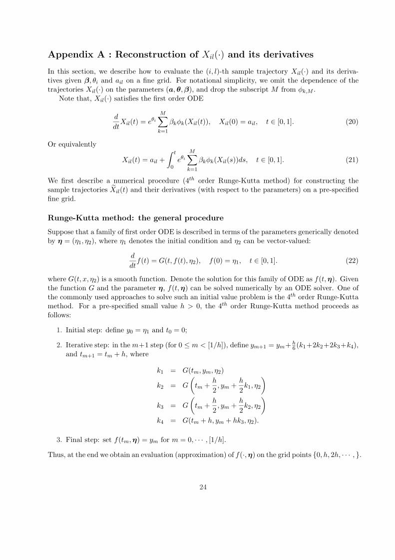
Appendix A : Reconstruction of Xil(·) and its derivatives

In this section, we describe how to evaluate the (i, l)-th sample trajectory Xil(·) and its deriva-tives given β, θi and ail on a fine grid. For notational simplicity, we omit the dependence of thetrajectories Xil(·) on the parameters (a, θ,β), and drop the subscript M from φk,M .

Note that, Xil(·) satisfies the first order ODE

d

dtXil(t) = eθi

M∑

k=1

βkφk(Xil(t)), Xil(0) = ail, t ∈ [0, 1]. (20)

Or equivalently

Xil(t) = ail +∫ t

0eθi

M∑

k=1

βkφk(Xil(s))ds, t ∈ [0, 1]. (21)

We first describe a numerical procedure (4th order Runge-Kutta method) for constructing thesample trajectories Xil(t) and their derivatives (with respect to the parameters) on a pre-specifiedfine grid.

Runge-Kutta method: the general procedure

Suppose that a family of first order ODE is described in terms of the parameters generically denotedby η = (η1, η2), where η1 denotes the initial condition and η2 can be vector-valued:

d

dtf(t) = G(t, f(t), η2), f(0) = η1, t ∈ [0, 1]. (22)

where G(t, x, η2) is a smooth function. Denote the solution for this family of ODE as f(t, η). Giventhe function G and the parameter η, f(t, η) can be solved numerically by an ODE solver. One ofthe commonly used approaches to solve such an initial value problem is the 4th order Runge-Kuttamethod. For a pre-specified small value h > 0, the 4th order Runge-Kutta method proceeds asfollows:

1. Initial step: define y0 = η1 and t0 = 0;

2. Iterative step: in the m+1 step (for 0 ≤ m < [1/h]), define ym+1 = ym+ h6 (k1+2k2+2k3+k4),

and tm+1 = tm + h, where

k1 = G(tm, ym, η2)

k2 = G

(tm +

h

2, ym +

h

2k1, η2

)

k3 = G

(tm +

h

2, ym +

h

2k2, η2

)

k4 = G(tm + h, ym + hk3, η2).

3. Final step: set f(tm, η) = ym for m = 0, · · · , [1/h].

Thus, at the end we obtain an evaluation (approximation) of f(·, η) on the grid points 0, h, 2h, · · · , .

24

Note that f(t, η) satisfies,

f(t, η) = η1 +∫ t

0G(s, f(s,η), η2)ds, t ≥ 0. (23)

Partially differentiating f(t, η) with respect to η and taking derivatives inside the integral, weobtain

∂

∂η1f(t, η) = 1 +

∫ t

0

∂

∂η1f(s,η)Gf (s, f(s,η), η2)ds, (24)

∂

∂η2f(t, η) =

∫ t

0

[∂

∂η2f(s,η)Gf (s, f(s,η), η2) + Gη(s, f(s,η), η2)

]ds, (25)

where Gf and Gη denote the partial derivatives of G with respect to its second and third arguments,respectively. In equations (24) and (25), if we view the f(·, η) inside Gf , Gη as known , ∂

∂η1f(t, η)

is the solution of the first order ODEd

dtp(t) = H(t, p(t), η2), p(0) = 1, t ∈ [0, 1],

where H(t, x, η2) = xGf (t, f(t, η), η2). Similarly, ∂∂η2

f(t,η) is the solution of the first order ODEwith p(0) = 0 and H(t, x, η2) = xGf (t, f(t, η), η2) + Gη(t, f(t,η), η2). Thus, given the functionG and the parameter η, a general strategy for numerically computing f(·, η) and its gradient∂

∂ηf(·, η) on a fine grid is to first use the Runge-Kutta method to approximate the solution to (23),and then using that approximate solution in place of f(·, η) in equations (24) and (25) to computethe gradients by another application of the Runge-Kutta method. Note that, if we evaluate f(·, η)on the grid points 0, h, 2h, · · · , by the above procedure, we will obtain the gradients ∂

∂ηf(·, η) ona rougher grid: 0, 2h, 4h, · · · .

Derivatives of the sample paths Xil(·) with respect to (a,θ,β)

Differentiating (20) with respect to the parameters, we have

Xailil (t) :=

∂Xil(t)∂ail

= 1 +∫ t

0

∂Xil(s)∂ail

eθi

M∑

k=1

βkφ′k(Xil(s))ds (26)

Xθiil (t) :=

∂Xil(t)∂θi

=∫ t

0

[∂Xil(s)

∂θieθi

M∑

k=1

βkφ′k(Xil(s)) + eθi

M∑

k=1

βkφk(Xil(s))

]ds (27)

Xβr

il (t) :=∂Xil(t)

∂βr=

∫ t

0

[∂Xil(s)

∂βreθi

M∑

k=1

βkφ′k(Xil(s)) + eθiφr(Xil(s))

]ds, (28)

for i = 1, · · · , n; l = 1, · · · , Ni; r = 1, · · · ,M . In another word, these functions satisfy the differentialequations:

d

dtXail

il (t) = Xailil (t)eθi

M∑

k=1

βkφ′k(Xi(t)), Xail

il (0) = 1, (29)

d

dtXθi

il (t) = Xθiil (t)eθi

M∑

k=1

βkφ′k(Xil(t)) + eθi

M∑

k=1

βkφk(Xil(t)), Xθiil (0) = 0, (30)

d

dtXβr

il (t) = Xβr

il (t)eθi

M∑

k=1

βkφ′k(Xil(t)) + eθiφr(Xil(t)), Xβr

il (0) = 0. (31)

25

Using similar arguments, it follows that the Hessian of Xil(·) with respect to β, given by the matrix(Xβr,βr′

il )Mr,r′=1, where X

βr,βr′il (t) := ∂2

∂βr∂βr′Xil(t), satisfies the system of ODEs, for r, r′ = 1, · · · ,M :

d

dtX

βr,βr′il (t) = eθi

[X

βr,βr′il (t)

M∑

k=1

βkφ′k(Xil(t)) + Xβr

il (t)φ′r′(Xil(t)) + Xβr′il (t)φ′r(Xil(t))

+ Xβr

il (t)Xβr′il (t)

M∑

k=1

βkφ′′k(Xil(t))

], X

βr,βr′il (0) = 0. (32)

The Hessian of Xil(·) with respect to θi, given by Xθi,θi

il , satisfies the ODE

d

dtXθi,θi

il (t) = eθi

[M∑

k=1

βkφk(Xil(t)) + (Xθi,θi

il (t) + 2Xθiil (t))

M∑

k=1

βkφ′k(Xil(t))

+ (Xθiil (t))2

M∑

k=1

βkφ′′k(Xil(t))

], Xθi,θi

il (0) = 0. (33)

The Hessian of Xil(·) with respect to ail, given by Xail,ailil , satisfies the ODE

d

dtXail,ail

il (t) = eθi

[Xail,ail

il (t)M∑

k=1

βkφ′k(Xil(t))

+ (Xailil (t))2

M∑

k=1

βkφ′′k(Xi(t))

], Xail,ail

il (0) = 0. (34)

Also, for future reference (even though it is not used in the proposed algorithm), we calculate themixed partial derivative of Xil(·) with respect to θi and βr as Xθi,βr

il (t) := ∂2Xil(t)∂θi∂βr

which satisfiesthe ODE

d

dtXθi,βr

il (t) = Xθi,βr

il (t)eθi

M∑

k=1

βkφ′k(Xil(t)) + eθi

[Xβr

il (t)M∑

k=1

βkφ′k(Xil(t)) + φr(Xil(t))

+ Xθiil (t)φ′r(Xil(t)) + Xθi

il (t)Xβr

il (t)M∑

k=1

βkφ′′k(Xil(t))

], Xθi,βr

il (0) = 0. (35)

Thus, the approach described above shows that as long as we have evaluated (approximated) thefunction Xil(·) at the grid points 0 + mh/2 : m = 0, 1, . . . , 2/h, we shall be able to approximatethe gradients Xail

il (·), Xθiil (·) and Xβr

il Mr=1 at the grid points 0+mh : m = 0, 1, . . . , 1/h, and the

Hessians Xail,ailil , Xθi,θi

il and (Xβr,βr′il )M

r,r′=1at the grid points 0 + 2mh : m = 0, 1, . . . , 1/(2h), bysuccessively applying the 4th order Runge-Kutta method.

Expression when g is positive

Note that (29), (30) and (31) are linear differential equations. For the growth model we haveg positive and the initial conditions ail also can be taken to be positive. If the function gβ :=∑M

k=1 βkφk is also positive on the domain of ail’s, then the trajectories Xil(t) are nondecreasingin t (in fact strictly increasing if gβ is strictly positive). In this case, and more generally, whenever

26

the solutions exist on a time interval [0, 1] and gβ is twice continuously differentiable (so thatthe solution paths for Xail

il , Xθilil , Xβr

il , Xail,ailil , Xθi,θi

il and Xβr,βr′il are C1 functions on [0, 1]) the

gradients of the trajectories can be solved explicitly:

Xailil (t) =

gβ(Xil(t))gβ(Xil(0))

; (36)

Xθiil (t) = eθitgβ(Xil(t)); (37)

Xβr

il (t) = gβ(Xil(t))∫ Xil(t)

Xil(0)

φr(x)(gβ(x))2

dx. (38)

In the following, we verify equation(38). The proofs for others are similar and thus omitted. Wecan express

Xβr

il (t) = eθi

∫ t

0φr(Xil(s)) exp

(eθi

∫ t

sg′β(Xil(u))du

)ds

= eθi

∫ t

0φr(Xil(s)) exp

(∫ t

s

g′β(Xil(u))gβ(Xil(u))

X ′il(u)du

)ds (using X ′

il(u) = eθigβ(Xil(u)) )

= eθi

∫ t

0φr(Xil(s)) exp(log gβ(Xil(t))− log gβ(Xil(s)))ds

= gβ(Xil(t))∫ t

0

φr(Xil(s))(gβ(Xil(s)))2

X ′il(s)ds

= gβ(Xil(t))∫ Xil(t)

Xil(0)

φr(x)(gβ(x))2

dx.

Using analogous calculations, we can obtain the Hessians in closed form as well. Thus, solutionsto (34), (33) and (32) become

Xail,ailil (t) =

gβ(Xil(t))(gβ(Xil(0)))2

[g′β(Xil(t))− g′β(Xil(0))]; (39)

Xθi,θi

il (t) = eθigβ(Xil(t))[t + eθit2g′β(Xil(t))]; (40)

Xβr,βr′il (t)

= gβ(Xil(t))∫ Xil(t)

Xil(0)

1gβ(x)

[φ′r(x)(Fr′(x)− Fr′(Xil(0))) + φ′r′(x)(Fr(x)− Fr(Xil(0)))

]dx

+(Fr(Xil(t))− Fr(Xil(0)))(Fr′(Xil(t))− Fr′(Xil(0)))gβ(Xil(t))g′β(Xil(t))

−e−θigβ(Xil(t))∫ Xil(t)

Xil(0)

g′β(x)(gβ(x))3

[φr(x)(Fr′(x)− Fr′(Xil(0))) + φr′(x)(Fr(x)− Fr(Xil(0)))] dx,

(41)

where, for x1 < x2,

Fr(x2)− Fr(x1) =∫ x2

x1

φr(y)(gβ(y))2

dy, 1 ≤ r ≤ M.

27

We can express Xβr,βr′il (t) alternatively as

Xβr,βr′il (t) = eθigβ(Xil(t))

∫ t

0

1gβ(Xil(s))

[Xβr

il (s)φ′r′(Xil(s)) + φ′r(Xil(s))Xβr′il (s)

]dt

+eθigβ(Xil(t))∫ t

0

1gβ(Xil(s))

Xβr

il (s)Xβr′il (s)g′′β(Xil(s))ds. (42)

Similarly, we have the representation

Xθi,βr

il (t) = eθigβ(Xil(t))∫ t

0

1gβ(Xil(s))

Xθiil (s)φ′r(Xil(s))ds

+eθigβ(Xil(t))∫ t

0

1gβ(Xil(s))

[Xβr

il (s)g′β(Xil(s)) + φr(Xil(s)) + Xθiil (s)Xβr

il (s)g′′β(Xil(s))]ds.

(43)

Appendix B : Levenberg-Marquardt method

The Levenberg-Marquardt method is a method for solving the nonlinear least squares problem:

minγ

S(γ) where S(γ) =n∑

i=1

[yi − fi(γ)]2,

where fi(γ)’s are nonlinear functions of the parameter γ ∈ Rp. The key idea is to linearly ap-proximate fi(γ + δ) ≈ fi(γ) + JT

i δ, for a small δ ∈ Rp, where Ji is the Jacobian of fi at γ.Denote

y = (y1, . . . , yn)T , f(γ) = (f1(γ), . . . , fn(γ))T ,

and J to be the n× p matrix with rows JT1 , . . . , JT

n . The resulting linearized least squares probleminvolves, for given γ solving for δ the equation

(JTJ + λ diag(JTJ))δ = JT (y − f(γ)), (44)

for a regularization parameter λ > 0. Note that, this solution bears similarity with the ridgeregression estimate. However, the formulation in (44) is according to the observation by Marquardtthat if each component of the gradient is scaled according to the curvature then there is a largermovement in the directions where the gradient is smaller. In practice, the regularization parameterλ is chosen adaptively to facilitate convergence.

Appendix C : Newton-Raphson procedure

We briefly describe the key steps of the Newton-Raphson procedure for optimizing the objectivefunction (6). As in the implementation of the Levenberg-Marquardt algorithm, we break theiterative procedure in three steps. The update of a is still performed by the Levenberg-Marquardtalgorithm (9), while keeping θ and β fixed at the current values. However, we employ Newton-Raphson to update θ and β. Fixing a, β at the current estimates a∗ and β∗, respectively, weupdate θi’s from the current estimates θ∗i by

θnewi = θ∗i −

Ni∑

l=1

mil∑

j=1

∂2`ilj

∂θ2i

−1

Ni∑

l=1

mil∑

j=1

∂`ilj

∂θi, (45)

28

where the quantities on the right hand side are all evaluated at (a∗,θ∗, β∗), and

∂`ilj

∂θi= −2εilj

∂

∂θiXil(tilj) + 2

λ2θi∑Nil=1 mil

∂2`ilj

∂θ2i

= −2εilj∂2

∂2θiXil(tijl) + 2(

∂

∂θiXil(tijl))2 + 2

λ2∑Nil=1 mil

.

Similarly, the Newton-Raphson update for β is given by

βnew = β∗ −

n∑

i=1

Ni∑

l=1

mil∑

j=1

∂2`ilj

∂β∂βT+ 2B

−1

n∑

i=1

Ni∑

l=1

mil∑

j=1

∂`ilj

∂β+ 2Bβ∗

, (46)

where the quantities on the right hand side are again evaluated at (a∗, θ∗, β∗), and

∂`ilj

∂β= −2εilj

∂

∂βXil(tilj)

∂2`ilj

∂β∂βT= 2

∂

∂βXil(tilj)

(∂

∂βXil(tilj)

)T

− 2εilj∂2

∂β∂βTXil(tilj).

Appendix D : Cubic B-spline fits to the plant data

We first consider the control group. In Table 4, we report the results using B-spline basis withknots at 1 + 11.5(1 : M)/M for M = 2, 3, · · · , 12; and using σini

ε = 0.05, and σiniθ = 1 as initial

estimates. In the B-spline fitting, we set the penalty matrix B to be the zero matrix, that isλR = 0. In the Newton-Raphson step, both λ1 and λ2 are estimated adaptively from the data.However, the Levenberg-Marquardt step is non-adaptive, that is it uses the initial values of λ1 andλ2 throughout. From Table 4, for M= 2 to 8 there is no convergence. For M = 9 to 12, theapproximate CV scores are quite similar and the minimum is achieved at M = 9.

We then consider the fits for the treatment group. The results using B-splines with knots at1 + 9.5(1 : M)/M for M = 2, 3, · · · , 12; and using σini

ε = 0.05, and σiniθ = 1 are reported in Table

5. We again set λR = 0 (that is no penalty). As for M = 2 to 6, there is no convergence. For M=7to 10, the CV scores are similar and the minimum is achieved again at M=9. For M = 11 and 12,the method breaks down due to numerical instability.

Appendix E : Proof details

In this section we provide the proofs of the key asymptotic results.

Proof of Theorem 1

For convenience, we introduce the following notations:

`i.(θi, β) :=Ni∑

l=1

mi∑

j=1

`ilj(ail, θi, β) and `..(θ, β) :=n∑

i=1

`i.(θi, β).

29

Table 4: Approximate leave-one-curve-out CV scores for control group. Cubic B-spline basis withknot sequence 1 + 11.5(1 : M)/M ; and σini

ε = 0.05, σiniθ = 1. (* = no convergence)

M # L-M # N-R CV score2* 216 1000 489.011623* 445 1000 416.698484* 458 1000 91.213085* 546 1000 74.125816* 337 1000 58.254877* 279 1000 53.692438* 190 1000 53.377219 233 195 53.1698710 147 120 53.2600811 94 79 53.2612512 78 54 53.41077

Table 5: Approximate leave-one-curve-out CV scores for treatment group. Cubic B-spline basiswith knot sequence 1 + 9.5(1 : M)/M ; and σini

ε = 0.05, σiniθ = 1. (* = no convergence)

M # L-M # N-R CV score2* 228 1000 348.658673* 426 1000 422.031374* 233 1000 96.662505* 257 1000 71.779046* 539 1000 65.852527 336 277 64.253708 197 143 63.918289 125 83 63.8334610 94 38 63.9000311* – – –12* – – –

30

Here, θ := (θ2, . . . , θn)T since θ1 ≡ 0. For α > 0, define

Ω(α) := (θ, β) : θ = θ∗ + αη, β = β∗ + αδ, η ∈ Rn−1, δ ∈ RM , s.t. ‖ η ‖2 + ‖ δ ‖2= 1. (47)

We use Xgilj to denote Xil(Ti,j ; ail, g) where Xil(·) is the solution of the equation x′(t) = eθ∗i g(x(t))

with x(0) = ail. We use Xil(·;θ, β) to denote the solution of (17) when Xil(0) = ail, andXilj(θ,β) := Xil(Ti,j ;θ, β). We define Xθi

il (·;θ, β), Xβr

il (·; θ, β), Xθi,θi

il (·;θ, β), Xθi,βr

il (·; θ, β) andX

βr,βr′il (·; θ, β) as the partial derivatives and mixed partial derivatives of Xil(·; θ,β) with respect

to θi, βr, (θi, θi), (θi, βr) and (βr, βr′), respectively. Notations such as Xθiilj(θ, β) are used to mean

Xθiil (Ti,j ;θ, β). We use gβ to denote the function

∑Mk=1 βkφk (for convenience henceforth dropping

the subscript M from φk,M ) and denote its first and second derivatives by g′β and g′′β, respectively.Finally, we use ‖ · ‖∞ to mean ‖ · ‖L∞(D), and denote the operator norm of a matrix and l2 normof a vector by ‖ · ‖. We use T to denote Ti,j : j = 1, . . . ,mi; i = 1, . . . , n and ε to denoteεilj : j = 1, . . . , mi; l = 1, . . . , Ni; i = 1, . . . , n.

Let η ∈ Rn−1 and δ ∈ RM be arbitrary vectors satisfying ‖ η ‖2 + ‖ δ ‖2= 1. DefineJn−1 := In−1 − 1

n−11n−11Tn−1 and observe that

∑ni=2(θi − θ)2 = θT Jn−1θ. Define

Wβ :=n∑

i=1

Ni∑

l=1

mi∑

j=1

(Yilj −Xil(Ti,j ; ail, θ∗i ,β

∗))∂Xil

∂β(Ti,j ; ail, θ

∗i , β

∗)

and Wθ to be an (n− 1)× 1 vector with (i− 1)-th coordinate

Ni∑

l=1

mi∑

j=1

(Yilj −Xil(Ti,j ; ail, θ∗i , β

∗))∂Xil

∂θi(Ti,j ; ail, θ

∗i , β

∗)

for i = 2, . . . , n. Also let W := (W Tβ ,W T

θ )T . Then by a second order Taylor expansion, we have,

`..(θ∗ + αNη, β∗ + αNδ)− `..(θ∗, β∗)

= λ2αN (2(θ∗)T Jn−1η + αNηT Jn−1η) + 2αN [δT ,ηT ][Wβ

Wθ

]

+α2N [δT ,ηT ]

[Gββ(θ, β) Gβθ(θ, β)Gθβ(θ, β) Gθθ(θ, β)

] [δη

]

−α2N [δT ,ηT ]

[Hββ(θ, β) Hβθ(θ,β)Hθβ(θ, β) Hθθ(θ,β)

] [δη

], (48)

where (θ,β) satisfies ‖ β−β∗ ‖≤ αN and ‖ θ−θ∗ ‖≤ αN . Note that (θ,β) depends on (a, T ) and(η, δ), but not on ε. In the above, Gββ(θ, β) is the M ×M matrix

n∑

i=1

Ni∑

l=1

mi∑

j=1

(∂Xil

∂β(Ti,j ; ail, θi, β)

)(∂Xil

∂β(Ti,j ; ail, θi,β)

)T

;

Gθβ(θ,β) is the (n− 1)×M matrix with (i− 1)-th row

Ni∑

l=1

mi∑

j=1

∂Xil

∂θi(Ti,j ; ail, θi,β)

(∂Xil

∂β(Ti,j ; ail, θi, β)

)T

, i = 2, . . . , n;

31

Gθθ(θ, β) is the (n− 1)× (n− 1) diagonal matrix with the (i− 1)-th diagonal entry

Ni∑

l=1

mi∑

j=1

(∂Xil

∂θi(Ti,j ; ail, θi, β)

)2

, i = 2, . . . , n;

Gβθ(θ,β) = Gθβ(θ,β)T ; Hββ(θ, β) is the M ×M matrix

n∑

i=1

Ni∑

l=1

mi∑

j=1

(Yilj −Xil(Ti,j ; ail, θi, β))∂2Xil

∂β∂βT(Ti,j ; ail, θi,β);

Hθβ(θ,β) is the (n− 1)×M matrix with (i− 1)-th row

Ni∑

l=1

mi∑

j=1

(Yilj −Xil(Ti,j ; ail, θi, β))∂2Xil

∂θi∂βT(Ti,j ; ail, θi, β), i = 2, . . . , n;

Hθθ(θ, β) is the (n− 1)× (n− 1) matrix with (i− 1)-th diagonal entry

Ni∑

l=1

mi∑

j=1

(Yilj −Xil(Ti,j ; ail, θi, β))∂2Xil

∂θ2i

(Ti,j ; ail, θi, β), i = 2, . . . , n;

andHβθ(θ, β) = Hθβ(θ, β)T . Let G∗,θθ, G∗,βθ, G∗,θβ and G∗,ββ denote the expectations of Gθθ(θ∗, β∗),Gβθ(θ∗,β∗), Gθβ(θ∗, β∗) and Gββ(θ∗,β∗) with respect to (a, T ). For future reference, we define the(M + n− 1)× (M + n− 1) symmetric matrix G(θ,β) as

G(θ, β) =[Gββ(θ,β) Gβθ(θ,β)Gθβ(θ, β) Gθθ(θ, β)

].

We define H(θ, β) and G∗ analogously.The following decomposition of the residuals is used throughout:

Yilj −Xilj(θ,β) = εilj + (Xgilj −Xilj(θ∗, β∗)) + (Xilj(θ∗,β∗)−Xilj(θ, β)). (49)

Without loss of generality in the following we assume that αNM3/2 → 0, so that in particular thebounds (61) - (69) are valid. The proof of Theorem 1 then follows from the following sequence oflemmas.

Lemma A.1 : Let γ = (δT , ηT )T , and W be as defined earlier. Then, with probability tending to1, uniformly in γ such that ‖ γ ‖= 1, we have

|γT W | =[O(σεM

1/2√

log(Nm)) + O(M−p(Nm)1/2)]√

γTG(θ∗,β∗)γ. (50)

Lemma A.2 : With γ as in Lemma A.1, uniformly over γ, we have

γT

[Gββ(θ, β)− Gββ(θ∗,β∗) Gβθ(θ,β)− Gβθ(θ∗, β∗)Gθβ(θ, β)− Gθβ(θ∗, β∗) Gθθ(θ,β)− Gθθ(θ∗, β∗)

]γ

= O(αNM3/2(Nm)1/2)√

γTG(θ∗, β∗)γ + O(α2NM3Nm). (51)

32

Lemma A.3 : There exists a constant c7 > 0 such that, with γ as in Lemma A.1, uniformly overγ, we have

γTG(θ∗,β∗)γ ≥ γTG∗γ(1− oP (1)) ≥ c7κ−1M Nm(1− oP (1)). (52)

Lemma A.4 : With γ as in Lemma A.1, with probability tending to 1, uniformly over γ,

γT

[Hββ(θ, β)−Hββ(θ∗, β∗) Hβθ(θ, β)−Hβθ(θ∗, β∗)Hθβ(θ, β)−Hθβ(θ∗, β∗) Hθθ(θ, β)−Hθθ(θ∗,β∗)

]γ

= O(αNM3/2(Nm)1/2)√

γTG∗γ + O(αNM1/2Nm) + O(α2NM3Nm)

+O(αNM5/2−pNm) + O(σεαNM3(Nm)1/2√

log(Nm)). (53)

Finally, using (49), (60), and (65)-(69), we have

max‖ Hββ(θ∗, β∗) ‖, ‖ Hβθ(θ∗,β∗) ‖, ‖ Hθθ(θ∗, β∗) ‖= OP (σεM(Nm)1/2) + O(M−(p−1)Nm). (54)

Combining (51) - (54), from (48), with probability tending to 1, uniformly in γ,

`..(θ∗ + αNη, β∗ + αNδ)− `..(θ∗, β∗)≥ α2

NγTG(θ∗,β∗)γ

−αN

(O(σεM

1/2√

log(Nm)) + O(M−p(Nm)1/2) + O(α2NM3/2(Nm)1/2)

)√γTG(θ∗, β∗)γ

−αNλ2 ‖ θ∗ ‖ O(1)− α2NO(αNM3/2(Nm)1/2)

√γTG∗γ

−α2NO((αNM1/2 + α2

NM3 + αNM5/2−p + M−(p−1))Nm)

−α2NO((σεαNM3 + σεM)(Nm)1/2

√log(Nm))

≥ c4κ−1M α2

NNm(1− oP (1)) (55)

where c4 > 0 is some constant. The last step uses Lemma A.3 and the following fact:

[Q ] For any positive definite matrix A, with ‖ A−1 ‖≤ κ, if 2c√

κ < 1, then for all x such that‖ x ‖= 1

xT Ax− c√

xT Ax ≥ 12xT Ax

Thus, with probability tending to 1, there is a local minimum (θ, β) of the objective function (5)with ‖ θ − θ∗ ‖2 + ‖ β − β∗ ‖2≤ α2

N . This completes the proof of Theorem 1.

Proof of Theorem 2

We make use of the following inequality due to Halperin and Pitt (Mitrinovic, Pecaric and Fink,1991, page 8): If f is locally absolutely continuous and f ′′ is in L2([0, A]), then for any ε > 0 thefollowing inequality holds ∫ A

0f ′2 ≤ K(ε)

∫ A

0f2 + ε

∫ A

0f ′′2

33

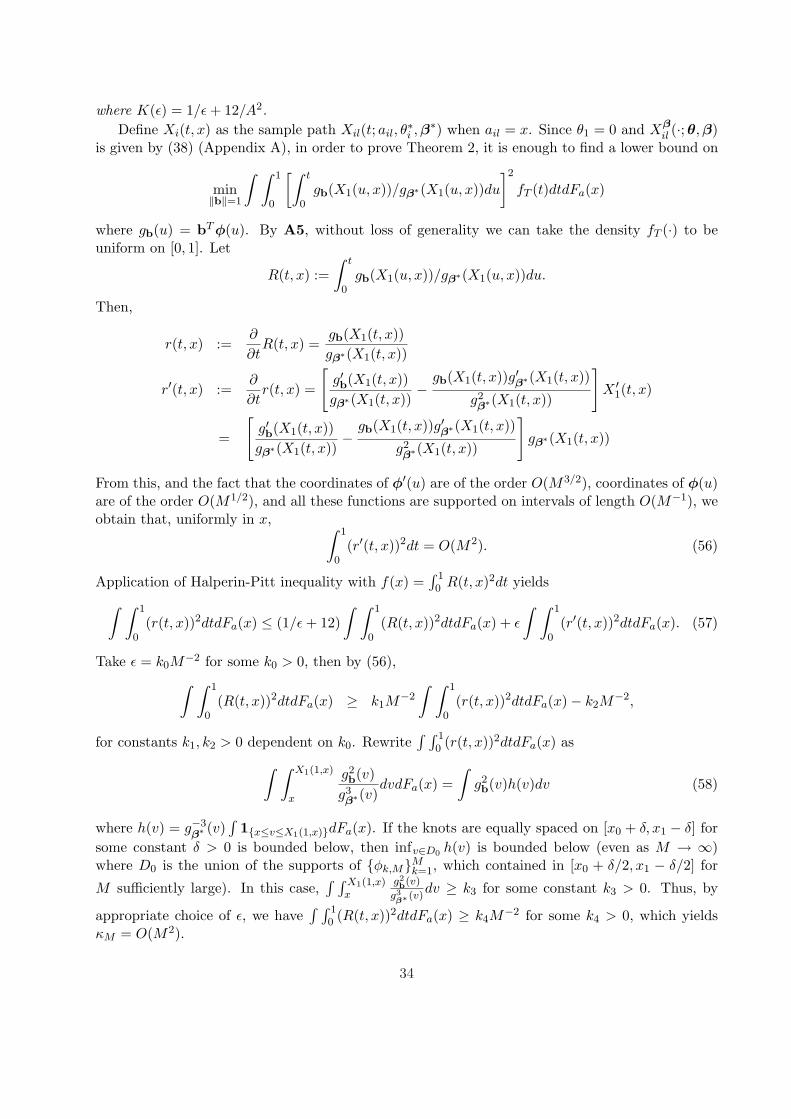
where K(ε) = 1/ε + 12/A2.Define Xi(t, x) as the sample path Xil(t; ail, θ

∗i , β

∗) when ail = x. Since θ1 = 0 and Xβil (·; θ, β)

is given by (38) (Appendix A), in order to prove Theorem 2, it is enough to find a lower bound on

min‖b‖=1

∫ ∫ 1

0

[∫ t

0gb(X1(u, x))/gβ∗(X1(u, x))du

]2

fT (t)dtdFa(x)

where gb(u) = bT φ(u). By A5, without loss of generality we can take the density fT (·) to beuniform on [0, 1]. Let

R(t, x) :=∫ t

0gb(X1(u, x))/gβ∗(X1(u, x))du.

Then,

r(t, x) :=∂

∂tR(t, x) =

gb(X1(t, x))gβ∗(X1(t, x))

r′(t, x) :=∂

∂tr(t, x) =

[g′b(X1(t, x))gβ∗(X1(t, x))

−gb(X1(t, x))g′β∗(X1(t, x))

g2β∗(X1(t, x))

]X ′

1(t, x)

=

[g′b(X1(t, x))gβ∗(X1(t, x))

−gb(X1(t, x))g′β∗(X1(t, x))

g2β∗(X1(t, x))

]gβ∗(X1(t, x))

From this, and the fact that the coordinates of φ′(u) are of the order O(M3/2), coordinates of φ(u)are of the order O(M1/2), and all these functions are supported on intervals of length O(M−1), weobtain that, uniformly in x, ∫ 1

0(r′(t, x))2dt = O(M2). (56)

Application of Halperin-Pitt inequality with f(x) =∫ 10 R(t, x)2dt yields

∫ ∫ 1

0(r(t, x))2dtdFa(x) ≤ (1/ε + 12)

∫ ∫ 1

0(R(t, x))2dtdFa(x) + ε

∫ ∫ 1

0(r′(t, x))2dtdFa(x). (57)

Take ε = k0M−2 for some k0 > 0, then by (56),

∫ ∫ 1

0(R(t, x))2dtdFa(x) ≥ k1M

−2

∫ ∫ 1

0(r(t, x))2dtdFa(x)− k2M

−2,

for constants k1, k2 > 0 dependent on k0. Rewrite∫ ∫ 1

0 (r(t, x))2dtdFa(x) as

∫ ∫ X1(1,x)

x

g2b(v)

g3β∗(v)

dvdFa(x) =∫

g2b(v)h(v)dv (58)

where h(v) = g−3β∗ (v)

∫1x≤v≤X1(1,x)dFa(x). If the knots are equally spaced on [x0 + δ, x1 − δ] for

some constant δ > 0 is bounded below, then infv∈D0 h(v) is bounded below (even as M → ∞)where D0 is the union of the supports of φk,MM

k=1, which contained in [x0 + δ/2, x1 − δ/2] for

M sufficiently large). In this case,∫ ∫ X1(1,x)

x

g2b(v)

g3β∗ (v)

dv ≥ k3 for some constant k3 > 0. Thus, by

appropriate choice of ε, we have∫ ∫ 1

0 (R(t, x))2dtdFa(x) ≥ k4M−2 for some k4 > 0, which yields

κM = O(M2).

34

Proof of Proposition 1

The proof is based on the following lemmas.

Lemma A.5: Let Pd be the class of all polynomials p(x) =∑d

j=0 βjxj of degree d on [0, 1] such

that |p|∞ = 1. Then there exists a constant c > 0 such that

|p|∞ ≥ c max0≤j≤d

|βj |.

Lemma A.6: Let µ be a measure on the interval [0, 1] with the property that for any L > 0, thereexists a constant C(L) > 0 such that for any interval A ⊂ [0, 1], µ(B)/µ(A) ≥ C(L) for all intervalsB ⊂ A with length(B)/length(A) ≥ L. Then for any polynomial p of degree d on [0, 1], there existsa constant c > 0 such that ∫

Ap2dµ ≥ c sup

u∈A|p(u)|2µ(A).

For the next lemma, assume that the knots are t1 = · · · = td+1 = 0, tM+1 = · · · = tM+d+1 = 1and 0 < td+2 < · · · < tM < 1. Note that we have placed extra knots at 0 and 1 in order to obtaina B-spline basis. Let ψ := ψj : j = 1, ..., M be the (unnormalized) B-spline basis with the knotstj : j = d + 2, ..., M. Let β ∈ RM , and consider the spline s(x) :=

∑Mj=1 βjψj(x). Then on the

interval Ai := [ti, ti+1], s(x) =∑

i−d≤j≤i βjψj(x) with∑

i−d≤j≤i ψj(x) = 1.

Lemma A.7: Assume that µ is a measure on [0, 1] satisfying the properties of Lemma A.6 above.Consider the vector ψ of B-splines on [0, 1] of degree d with well-conditioned knots at td+2, ..., tM ,i.e., the sequence M(ti+1−ti) : i = d+1, ...,M remains bounded between two positive constants forany M . Then there exist constants c12, c13 > 0 (which do not depend on td+2, ..., tM ) such that all theeigenvalues of the matrix

∫ψψT dµ are between c12 mind+1≤i≤M µ(Ai) and c13 maxd+1≤i≤M µ(Ai).

Lemma A.8: Let h be a bounded nonnegative function on [0, 1] which is bounded away from zeroexcept perhaps near 0 and 1. Assume that limx→0 x−γh(x) and limx→1(1 − x)−γh(x) are positiveconstants for some 0 < γ ≤ 1. Let ψ be a (unnormalized) B-spline basis (as in Lemma A.7). Thenall the eigenvalues of

∫ψψT hdx are bounded between c10M

−1−γ and c11M−1 for some positive

constants c10, c11 > 0.

Observe that under the stated condition on the density of Fa in the proposition, the function h(v)appearing in (58) has the same behavior as stated in Lemma A.8 (after a change of location andscale). Proposition 1 now follows from using Halperin-Pitt inequality as in (57), but now takingε ∼ M−2−γ .

Rate bounds

In this subsection, we summarize approximations of various quantities that are useful in provingLemmas A.1-A.4. First, by A3 we have the following:

‖ g(j)β − g

(j)β∗ ‖∞= O(αNM j+1/2) if ‖ β − β∗ ‖≤ αN , j = 0, 1, 2. (59)

Next, from A3 and A4, for M large enough, solutions Xil(t;θ,β) : t ∈ [0, 1] exist for all (θ, β)such that max‖ θ − θ∗ ‖, ‖ β − β∗ ‖ ≤ αN . This also implies that the solutions Xθi

il (·; θ,β),Xβr

il (·;θ, β), Xθi,θi

il (·;θ, β), Xθi,βr

il (·; θ,β) and Xβr,βr′il (·; θ, β) exist on [0, 1] for all (θ, β) such that

35

max‖ θ − θ∗ ‖, ‖ β − β∗ ‖ ≤ αN , since the latter are linear differential equations where thecoefficient functions depend on Xil(t; θ, β) (see Appendix A). Moreover, by Gronwall’s lemma(Lemma F.1), (59) and the fact that ‖ g

(j)β∗ ‖∞= O(1) for j = 0, 1, 2 (again by A3), all these

solutions are bounded for all θi and ail, by compactness of supp(Fa).Hence, if αNM3/2 = o(1), then using Corollary F.2 (in Appendix F), the fact that ‖ g

(j)β∗ ‖∞=

O(1) for j = 0, 1, 2, and the expressions for the ODEs for the partial and mixed partial derivatives(see Appendix A), after some algebra we obtain the following (almost surely):

‖ Xil(·;θ∗, β∗)−Xgil(·) ‖∞= O(M−p). (60)

The same technique can be used to prove the following (almost surely):

‖ Xil(·;θ, β)−Xil(·; θ∗, β∗) ‖∞ = O(αNM1/2) (61)‖ Xθi

il (·; θ,β)−Xθiil (·; θ∗, β∗) ‖∞ = O(αNM3/2) (62)

max1≤r≤M

‖ Xβr

il (·; θ∗, β∗) ‖∞ = O(M−1/2) (63)

max1≤r≤M

‖ Xβr

il (·;θ, β)−Xβr

il (·; θ∗, β∗) ‖∞ = O(αNM) (64)

‖ Xθi,θi

il (·; θ, β)−Xθi,θi

il (·; θ∗, β∗) ‖∞ = O(αNM5/2) (65)

max1≤r≤M

‖ Xθi,βr

il (·; θ∗, β∗) ‖∞ = O(M1/2) (66)

max1≤r≤M

‖ Xθi,βr

il (·; θ,β)−Xθi,βr

il (·; θ∗, β∗) ‖∞ = O(αNM2) (67)

max1≤r,r′≤M

‖ Xβr,βr′il (·; θ∗, β∗) ‖∞ = O(1) (68)

max1≤r,r′≤M

‖ Xβr,βr′il (·; θ,β)−X

βr,βr′il (·; θ∗, β∗) ‖∞ = O(αNM3/2) (69)

whenever max‖ θ − θ∗ ‖, ‖ β − β∗ ‖ ≤ αN .To illustrate the key arguments, we prove (63) and (64). By (38), and the fact that ‖ φr ‖∞=

O(M1/2) and is supported on an interval of length O(M−1), (63) follows; in fact it holds for all(θ,β) ∈ Ω(αN ) with Ω(α) as defined in (47). Next, note that the function φr is Lipschitz withLipschitz constant O(M3/2) and is supported on an interval of length O(M−1). Since (31) (inAppendix A) is a linear differential equation, using Corollary F.2 with

δf(t, x)

= x[eθig′β(Xil(t;θ, β))− eθ∗i g′β∗(Xil(t;θ∗, β∗))

]+ eθiφr(Xil(t; θ, β))− eθ∗i φr(Xil(t; θ∗,β∗))

= (eθi − eθ∗i )[xg′β(Xil(t; θ, β)) + φr(Xil(t;θ, β))

]+ xeθ∗i (g′β(Xil(t; θ, β))− g′β(Xil(t; θ∗, β∗)))

+xeθ∗i (g′β(Xil(t; θ∗,β∗)))− g′β∗(Xil(t; θ∗, β∗))) + eθ∗i (φr(Xil(t; θ, β))− φr(Xil(t;θ∗, β∗))),

we obtain (64) by using (61) and the following facts: on [0, 1], |Xβr

il (t)| = O(M−1/2) for all (θ, β) ∈Ω(αN ); ‖ g′′β ‖∞= O(αNM5/2); ‖ g′β − g′β∗ ‖∞= O(αNM3/2); and αNM3/2 = o(1).

Proof of lemmas

Proof of Lemma A.1 : Using (49), write

D1(γ) := γT W =n∑

i=1

Ni∑

l=1

mi∑

j=1

(εilj + ∆ilj)γTvilj ,

36

where ∆ilj := Xgilj − Xilj(θ∗,β∗), and vilj is the (M + n − 1) × 1 vector with the first M co-

ordinates given by vβilj := Xβ

il (Ti,j ; ail, θ∗i , β

∗), and the last (n − 1) coordinates given by vθilj :=

Xθiil (Ti,j ; ail, θ

∗i , β

∗)ei−1, where ei is the i-th canonical basis vector in Rn−1, and e0 := 0n−1. Noticethat G(θ∗, β∗) =

∑ni=1

∑Nil=1

∑mij=1 viljvT

ilj . Thus, by Cauchy-Schwarz inequality, and the fact thatmaxi,l,j |∆ilj | = O(M−p) (by (60)) we have, uniformly in γ,

|n∑

i=1

Ni∑

l=1

mi∑

j=1

∆iljγTvilj | = O(M−p(Nm)1/2)

√γTG(θ∗,β∗)γ.

Since εilj are i.i.d. N(0, σ2ε), we also have

n∑

i=1

Ni∑

l=1

mi∑

j=1

εiljγTvilj ∼ N(0, σ2

εγTG(θ∗,β∗)γ)

conditional on (a,T). Since the (conditional) Gaussian process

f(γ) :=

∑ni=1

∑Nil=1

∑mij=1 εiljγ

Tvilj

σε

√γTG(θ∗, β∗)γ

is a smooth function over SM+n−1 (the unit sphere centered at 0 in RM+n−1), and since by as-sumption M = O((Nm)d) for some d > 0, using a covering of the sphere SM+n−1 by balls of radiusεM ∼ (Nm)−D for an appropriately chosen D > 0, and using the fact that P (N(0, 1) > t) ≤t−1(2π)−1/2 exp(−t2/2), for t > 0, we conclude that uniformly in γ,

n∑

i=1

Ni∑

l=1

mi∑

j=1

εiljγTvilj = O(σεM

1/2√

log(Nm))√

γTG(θ∗, β∗)γ

except on a set with probability converging to zero. This completes the proof of the lemma.

Proof of Lemma A.2 : Define uilj the same way as vilj is defined in the proof of Lemma A.1,with (θ∗,β∗) replaced by (θ, β). Express D2(γ) := γT (G(θ, β)− G(θ∗,β∗))γ as

γT

n∑

i=1

Ni∑

l=1

mi∑

j=1

uiljuTilj −

n∑

i=1

Ni∑

l=1

mi∑

j=1

viljvTilj

γ

= γT

n∑

i=1

Ni∑

l=1

mi∑

j=1

((uilj − vilj)vTilj + (uilj − vilj)(uilj − vilj)T + vilj(uilj − vilj)T )

γ.

Then, by Cauchy-Schwarz inequality and (62) and (64), and the arguments used in the proof ofLemma A.1,

|D2(γ)| = O(αNM3/2(Nm)1/2)√

γTG(θ∗,β∗)γ + O(α2NM3Nm).

Proof of Lemma A.3 : Define D3(γ) := γT (G(θ∗,β∗)− G∗)γ. Then

D3(γ) =n∑

i=1

Ni∑

l=1

mi∑

j=1

uilj(γ) +n∑

i=1

Ni∑

l=1

mi∑

j=1

wilj(γ),

37

where uilj(γ) = γT (∇iXilj∇iXTilj−E[(∇iXilj∇iX

Tilj)|ail])γ and wilj(γ) = γT (E[(∇iXilj∇iX

Tilj)|ail]−

E[∇iXilj∇iXTilj)])γ, where, for notational simplicity,

∇iXilj =

[Xβ

il (Ti,j)Xθi

il (Ti,j)ei−1

], i = 1, . . . , n.

Note that, the random variables uilj(γ) have zero conditional mean (given ail), are uniformlybounded and the variables Zij(γ) :=

∑Nil=1 uilj(γ) are independent. Similarly, the random variables

wilji,j have zero mean are uniformly bounded and the variables∑mi

j=1 wilj(γ) are independent.Indeed, for each fixed (i, l), the variables wiljmi

j=1 are identical since Ti,j are i.i.d. Moreover, the col-lections uilj(γ) and wilj(γ) are differentiable functions of γ. Define G∗(a) := E(G∗(θ∗, β∗)|a).Then, since Zij(γ) are uniformly bounded by K1N for some constant K1 > 0, and are independentgiven a, we have

Var(n∑

i=1

mi∑

j=1

Zij(γ)|a) =n∑

i=1

mi∑

j=1

E[(Zij(γ))2|a]

≤n∑

i=1

mi∑

j=1

Ni

Ni∑

l=1

E[u2ilj(γ)|ail]

≤ K2Nn∑

i=1

Ni∑

l=1

mi∑

j=1

E[|uilj(γ)||ail] ≤ 2K2NγTG∗(a)γ.

In the above, second inequality uses (∑N

i=1 xi)2 ≤ N∑N

i=1 x2i , and the last follows from fact that

uilj(γ) is a difference of two nonnegative quantities, the second one being the conditional expec-tation of the first one given a. Thus, applying Bernstein’s inequality, for every v > 0, for everyγ ∈ SM+n−1,

P(|n∑

i=1

Ni∑

l=1

mi∑

j=1

uilj(γ)| > v|a) ≤ 2 exp(− v2/2

2K2NγTG∗(a)γ + K1Nv/3

).

Thus, using an entropy argument as in the proof of Lemma A.1, we conclude that given δ > 0 thereexist positive constants C1(δ) and C2(δ) such that on the set a|γTG∗(a)γ ≥ C2(δ)NM log(Nm),

P

(sup

γ∈SM+n−1

|∑ni=1

∑Nil=1

∑mij=1 uilj(γ)|√

γTG∗(a)γ> C1(δ)(NM log(Nm))1/2 | a

)≤ (Nm)−δ. (70)

On the other hand, using an inversion formula for block matrices,

‖ G−1∗ ‖ = ‖

[G∗,ββ G∗,βθ

G∗,θβ G∗,θθ

]−1

‖

= ‖[

C−1∗ −C−1∗ G∗,βθ(G∗,θθ)−1

−(G∗,θθ)−1G∗,θβC−1∗ (G∗,θθ)−1 + (G∗,θθ)−1G∗,θβC−1∗ G∗,βθ(G∗,θθ)−1

]‖

= O(κM (Nm)−1), (71)

38

where C∗ := G∗,ββ −G∗,βθ(G∗,θθ)−1G∗,θβ. The last equality in (71) is because A6 together with (63)implies in particular that ‖ G∗,βθ(G∗,θθ)−1 ‖= O(1). Now, from the facts that

γTG∗γ ≥ K3Nm

κM(by (71)) and minN,m À κMM log(Nm),

for some constant K3 > 0, so that γTG∗γ À mM log(Nm), and using arguments similar to thoseleading to (70) we have, for some C3(δ) > 0,

P

(sup

γ∈SM+n−1

|∑ni=1

∑Nil=1

∑mij=1 wilj(γ)|√

γTG∗γ> C3(δ)(mM log(Nm))1/2

)≤ (Nm)−δ. (72)

Now, observing that∑n

i=1

∑Nil=1

∑mij=1 wilj(γ) = γTG∗(a)γ−γTG∗γ, using fact [Q], and combining

with (70) and (72), we obtain that, there is a C4(δ) > 0 such that

P

(sup

γ∈SM+n−1

|D3(γ)|√γTG∗γ

≥ C4(δ)(m1/2 + N1/2)(M log(Nm))1/2

)= O((Nm)−δ). (73)

(Note that, if the time points tilj were independently and identically distributed for different

curves (i, l), then quantity (m1/2+N1/2)(M log(Nm))1/2 in (73) can be replaced by (M log(Nm))1/2).

From (73) it follows that

γTG(θ∗,β∗)γ ≥ γTG∗γ(1− oP (1)) ≥ c6κ−1M Nm(1− oP (1))

for some constant c6 > 0 and for sufficiently large N .

Proof of Lemma A.4 : Using (42) and (43) in Appendix A, for any t, we can express the(M + n − 1) × (M + n − 1) matrix with blocks Xβ,βT

il (t) := ((Xβr,βr′il (t)))M

r,r′=1, ei−1Xθi,β

T

il (t),

Xβ,θi

il (t)eTi−1 and Xθi,θi

il (t), as Uil(t) + Uil(t)T + Vil(t) where

Uil(t) = eθigβ(Xil(t))∫ t

0

1gβ(Xil(s))

[Xβ

il (s)Xθi

il (s)ei−1

][φ′(Xil(s))

0n−1

]T

ds (74)

and ‖ Vil(t) ‖= O(1) uniformly in t, i and l. Note that, in the above description, all the samplepaths and their derivatives are evaluated at (θ∗,β∗).

Observe that, since Yilj −Xil(Ti,j ; θ∗, β∗) = εilj + ∆ilj , where ∆ilj is as in the proof of LemmaA.1, we have

H(θ, β)−H(θ∗, β∗)

=n∑

i=1

Ni∑

l=1

mi∑

j=1

(Xilj(θ∗,β∗)−Xilj(θ, β))

[Xβ,βT

ilj (θ, β) Xβ,θi

ilj (θ, β)eTi−1

ei−1Xθi,β

T

ilj (θ,β) Xθi,θi

ilj (θ, β)ei−1eTi−1

]

+n∑

i=1

Ni∑

l=1

mi∑

j=1

(εilj + ∆ilj) ·[

Xβ,βT

ilj (θ, β)−Xβ,βT

ilj (θ∗, β∗) (Xβ,θi

ilj (θ, β)−Xβ,θi

ilj (θ∗, β∗))eTi−1

ei−1(Xθi,β

T

ilj (θ, β)−Xθi,βT

ilj (θ∗, β∗)) (Xθi,θi

ilj (θ,β)−Xθi,θi

ilj (θ∗, β∗))ei−1eTi−1

]. (75)

39

First break the last summation in the last term of (75) into two parts – one corresponding to∆ilj ’s and the other corresponding to εilj ’s. Then, using (60), (65), (67) and (69), we concludethat the sum involving ∆ilj is O(αNM5/2−pNm). The summation involving εilj ’s can be expressedas a linear function of ε with coefficients that are functions of a, T and γ, and depend smoothlyon γ. From this, conditionally on (a,T ), this term is coordinatewise normally distributed withstandard deviation O(σεαNM5/2(Nm)1/2) for each fixed γ. We can conclude from this by anentropy argument (similar to the one used in the proof of Lemma A.1) that the supremum of this

term over all γ ∈ SM+n−1 is O(σεαNM3(Nm)1/2√

log(Nm)) with probability tending to 1.Next, using (74) we express the first term of (75) as

n∑

i=1

Ni∑

l=1

mi∑

j=1

(Xilj(θ∗,β∗)−Xilj(θ,β))[Uil(tilj) + Uil(tilj)T + Vil(tilj)

]

+n∑

i=1

Ni∑

l=1

mi∑

j=1

(Xilj(θ∗,β∗)−Xilj(θ,β)) ·[

Xβ,βT

ilj (θ, β)−Xβ,βT

ilj (θ∗,β∗) (Xβ,θi

ilj (θ,β)−Xβ,θi

ilj (θ∗, β∗))eTi−1

ei−1(Xθi,β

T

ilj (θ,β)−Xθi,βT

ilj (θ∗, β∗)) (Xθi,θi

ilj (θ, β)−Xθi,θi

ilj (θ∗,β∗))ei−1eTi−1

]. (76)

The second sum is O(α2NM3Nm) by (61), (65), (67) and (69). Again, by (61), the contribution

in the first sum for the term involving Vil(tilj)’s is O(αNM1/2Nm). Finally, by Cauchy-Schwarzinequality, and (74), and the facts that gβ is bounded both above and below (for x ≥ x0), we havefor all 0 ≤ t ≤ 1,

|γT Uil(t)γ|2 ≤ cg

∫ t

0

(γT

[Xβ

il (s)Xθi

il (s)ei−1

])2

ds

∫ 1

0

(γT

[φ′(Xil(s))

0n−1

])2

ds,

for some constant cg > 0 depending on gβ∗ , θ and x0. Notice that∫

φ′(x)(φ′(x))T dx ≤ c7M2IM

for some c7 > 0. Furthermore,

supγ∈SM+n−1

supt∈[0,1]

∫ t

0

(γT

[Xβ

il (s)Xθi

il (s)ei−1

])2

ds = O(1).

These, together with an application of Cauchy-Schwarz inequality, and using manipulations asin the proof of Lemmas A.2 and A.3, shows that the sum involving the terms Uil(tilj)’s in theexpression (76) is O(αNM3/2(Nm)1/2)

√γTG∗γ. Lemma A.4 now follows.

Proof of Lemma A.5 : Suppose that the result is false. Then for any sequence of positiveconstant δn decreasing to zero, we can find a polynomial pn with coefficients βn,j , j = 0, ..., d,such that |pn|∞ ≤ δn max0≤j≤d |βn,j |. Let qn be the polynomial whose coefficients γn,j areobtained by dividing βj ’s by max0≤j≤d |βn,j |. Note that max |γn,j | = 1 for any n. By the usualcompactness argument we can find a subsequence of γn,j, which we continue to denote by γn,j,such that γn,j → γj , j = 0, ..., d, where maxj |γj | = 1. However the supremum norm of the limitingpolynomial q of degree d with coefficients γj is zero which implies that γj = 0 for all j. This leadsto a contradiction.

Proof of Lemma A.6 : Note that for any interval A = [a, b], a < b, we can write∫A p2dµ =∫ 1

0 q2dµA, where q(z) = p(a + (b− a)z) and dµA(z) = dµ(a + (b− a)z). Since |q|∞ = supu∈A |p(u)|,

40

we may take |q|∞ = 1. Let x∗ be a point in [0, 1] at which q(x∗) equals ±1. Then for any 0 ≤ x ≤ 1,q2(x) = 1 + (x− x∗)2q(x∗∗)q′′(x∗∗) for some x∗∗ in [0, 1]. Using Lemma A.5, we see that there is aconstant c14 such that |p′′|∞ ≤ c14 for all polynomials with |p|∞ = 1. So |q2(x)− 1| ≤ c14(x− x∗)2.So we can find an interval I ⊂ [0, 1] of length at least L = (2c14)−1/2 containing x∗ such thatq2(x) ≥ 1/2. Let B = a + (b− a)I. Then length(B)/length(A) = length(I) ≥ L. Consequently,

∫

Ap2dµ =

∫ 1

0q2dµA ≥ 1

2

∫

IdµA

=12µ(B) ≥ 1

2C(L)µ(A).

The result now follows.

Proof of Lemma A.7 : This result is clearly true for d = 0. We will prove it for the case d ≥ 1.Let β ∈ Rk and let s(x) = βT ψ(x). Since s is a convex combination of βi−d, ..., βi on the intervalAi, we have ∫

s2dµ =∑

d+1≤i≤M

∫ ti+1

ti

s2dµ ≤∑

d+1≤i≤M

∑

i−d≤j≤i

β2j µ(Ai).

This establishes the upper bound for the largest eigenvalue of∫

ψψT . We will now establish theresult on the lower bound of the smallest eigenvalue.

Using property (viii) in chapter XI in de Boor (1978), we know that supti+1≤x≤ti+d+1|s(x)| ≥

c15|βi| for all i for some constant c15 > 0. Denote m0 = mind+1≤i≤M µ(Ai). Hence for anyd ≤ i ≤ M , by Lemma A.6 we have

∫ ti+d+1

ti+1

s2dµ =∑

i+1≤j≤i+d+1

∫ tj+1

tj

s2dµ

≥ c∑

i+1≤j≤i+d+1

suptj≤x≤tj+1

|s(x)|2µ(Aj)

≥ c supti+1≤x≤ti+d+1

|s(x)|2m0 ≥ c16β2i m0.

Incidentally, the same type of inequality holds for any i = 1, .., d−1. Consequently we have∫

s2dµ ≥c17

∑β2

i m0 for some constant c17 > 0. This completes the proof.

Proof of Lemma A.8: This follows from Lemma A.7 once we take dµ(x) = h(x)dx.

Appendix F : Perturbation of Differential Equations

For nonparametric estimation of the gradient function g, we need to control the effect of lack offit to g (meaning that g may not be exactly represented in the given basis φk(·)) on the samplepaths Xil(t) : t ∈ [0, 1]. It is convenient to do this study under a general setting of first orderdifferential equations where the state variable x(·) is d-dimensional for d ≥ 1. Our aim is to controlthe perturbation of the sample paths and its derivatives with respect to the parameters governingthe differential equation when the true gradient function g is perturbed by an arbitrary functionδg(·).

We present two different results about the perturbation of the solution paths of the initial valueproblem:

x′ = f(t, x), x(t0) = x0, (77)

41

where x ∈ Rd, when the function f is perturbed by a smooth function.

Theorem F.1 (Deuflhard and Bornemann, 2002, p.80) : On the augmented phase space Ωlet the mappings f and δf be continuous and continuously differentiable with respect to the statevariable. Assume that for (t0, x0) ∈ Ω, the initial value problem (77), and the perturbed problem

x′ = f(t, x) + δf(t, x), x(t0) = x0, (78)

have the solutions x and x = x + δx, respectively. Then for t1 sufficiently close to t0, there exists acontinuous matrix-valued mapping M : ∆ → Rd×d on ∆ = (t, s) ∈ R2 : t ∈ [t0, t1], s ∈ [t0, t] suchthat the perturbation δx is represented by

δx(t) =∫ t

t0

M(t, s)δf(s, x(s))ds, for all t ∈ [t0, t1]. (79)

Note that, the point t1 can be chosen so that, the one-parameter family of initial value problems

x′ = f(t, x) + λ · δf(t, x), x(t0) = x0, (80)

has a corresponding solution φ(·;λ) ∈ C1([t0, t1],Rd) for each parameter value λ ∈ [0, 1]. Inparticular, φ(·; 0) = x(·) and φ(·; 1) = x(·).

Propagation matrix and its relationship to perturbation

Let Φt,t0 denote the map such that x(t) = Φt,t0x0 is the unique solution of the initial value problem(77). The following result (Theorem 3.1 in Deuflhard and Bornemann, 2002, p.77) describes thedependence of the map on the gradient function f .

Theorem F.2 : On the extended state space Ω let f be continuous and p-times continuouslydifferentiable, p ≥ 1, with respect to the state variable. Moreover, suppose that for (t0, x0) ∈ Ω theunique solution of the initial value problem (77) exists up to some time t > t0. Then there is aneighborhood of the the state x0 where for all s ∈ [t0, t1], the evolution

x → Φs,t0x

is p-times continuously differentiable with respect to the state variable. In other words, the evolutioninherits from the right side the smoothness properties with respect to the state variable.

Then, the linearized perturbation of the state, due to a perturbation δxs of the state at time s,namely,

δx(t) ≈ Φt,s(x(s) + δxs)− Φt,sx(s)

is given by δx(t) = W (t, s)δxs where

W (t, s) = DξΦt,sξ∣∣ξ=Φs,t0x0

∈ Rd×d (81)

is the Jacobi matrix. Note that, W (t, s) satisfies the differential equation:

d

dtW (t, s) = fx(t, Φt,t0x0)W (t, s), (82)

with initial condition W (s, s) = I. W (t, s) is called the propagation matrix belonging to x.

42

In general, we can express the matrix M(t, s) appearing in Theorem F.1 as

M(t, s) =∫ 1

0W (t, s; λ)dλ, (83)

where W (t, s;λ) is the propagation matrix belonging to φ(·; λ), and hence solves the homogeneousdifferential equation

d

dtW (t, s;λ) = fx(t, φ(t;λ))W (t, s; λ), W (s, s) = I.

From this, the following corollary follows easily.

Corollary F.1 : If the limit δf → 0 is uniform in a neighborhood of the graph of the solution x,then the linearization

δx(t) ≈∫ t

t0

W (t, s)δf(s, x(s))ds, for all t ∈ [t0, t1]

holds.

Gronwall’s Lemma and its implications

Lemma F.1 (Gronwall’s Lemma): Let ψ, χ ∈ C([t0, t1],R) be nonnegative functions and ρ ≥ 0.Then the integral inequality

ψ(t) ≤ ρ +∫ t

t0

χ(s)ψ(s)ds, for all t ∈ [t0, t1]

implies

ψ(t) ≤ ρ exp(∫ t

t0

χ(s)ψ(s)ds

)for all t ∈ [t0, t1].

In particular, ψ ≡ 0 holds for ρ = 0.

An immediate application of Lemma 1 is that, it gives a bound for ‖ W (t, s; λ) ‖. Indeed, if

‖ fx(t;φ(t; λ)) ‖≤ χ(t), for all λ ∈ [0, 1], (84)

then taking ψ(t) =‖ W (t, s;λ) ‖ (note that ψ(·) depends on s) and ρ =‖ W (s, s;λ) ‖=‖ I ‖= 1, weobtain

‖ W (t, s; λ) ‖≤ exp(∫ t

sχ(u)du

), for all t0 ≤ s < t ≤ t1, for all λ ∈ [0, 1]. (85)

Condition (84) holds in particular if ‖ fx(t, ·) ‖∞≤ χ(t), and then, from Theorem F.1, we obtainthe important result,

Corollary F.2 : If f is such that ‖ fx(t, ·) ‖∞≤ χ(t) for a function χ(·) bounded on [t0, t1], and‖ δf(t, ·) ‖∞≤ τ(t) for some nonnegative function τ(·) on [t0, t1], then

‖ δx(t) ‖≤∫ t

t0

exp(∫ t

sχ(u)du

)τ(s)ds, for all t ∈ [t0, t1]. (86)

Note that, even though M(t, s) in (79) in general depends on x0, the bound in (86) does not.This has the implication that if one can prove the existence of solutions φ(·;λ) : λ ∈ [0, 1] on aninterval [t0, t1] for an arbitrary collection of initial conditions x0, and the conditions of CorollaryF.2 hold, then the same perturbation bound (86) applies uniformly to each one of them.

43