Parameter Synthesis in Nonlinear Dynamical Systems:Application to Systems Biology

Alexandre Donze1, Gilles Clermont2,Axel Legay1, and Christopher J. Langmead1,3?

1 Computer Science Department, Carnegie Mellon University, Pittsburgh, PA2 Department of Critical Care Medicine, University of Pittsburgh, Pittsburgh, PA

3 Lane Center for Computational Biology, Carnegie Mellon University, Pittsburgh, PA

Abstract. The dynamics of biological processes are often modeled as systems of nonlinear ordinary differentialequations (ODE). An important feature of nonlinear ODEs is that seemingly minor changes in initial conditionsor parameters can lead to radically different behaviors. This is problematic because in general it is never possibleto know/measure the precise state of any biological system due to measurement errors. The parameter synthesisproblem is to identify sets of parameters (including initial conditions) for which a given system of nonlinear ODEsdoes not reach a given set of undesirable states. We present an efficient algorithm for solving this problem thatcombines sensitivity analysis with an efficient search over initial conditions. It scales to high-dimensional modelsand is exact if the given model is affine. We demonstrate our method on a model of the acute inflammatory responseto bacterial infection, and identify initial conditions consistent with 3 biologically relevant outcomes.

Key words: Verification, Nonlinear Dynamical Systems, Uncertainty, Systems Biology, Acute Illness

? Corresponding Author: cjl@cs.cmu.edu

1 Introduction

The fields of Systems Biology, Synthetic Biology, and Medicine produce and use a variety of formalisms formodeling the dynamics of biological systems. Regardless of its mathematical form, a model is an invaluabletool for thoroughly examining how the behavior of a system changes when the initial conditions are altered.Such studies can be used to generate verifiable predictions, and/or to address the uncertainty associated withexperimental measurements obtained from real systems.

In this paper, we consider the parameter synthesis problem which is to identify sets of parameters forwhich the system does (or does not) reach a given set of states. Here, the term “parameter” refers to boththe initial conditions of the model (e.g., bacterial load at time t = 0) and dynamical parameters (e.g., thebacterium’s doubling rate). For example, in the context of medicine, we might be interested in partitioningthe parameter space into two regions — those that, without medical intervention, deterministically lead tothe patient’s recovery, and those that lead to the patient’s death. The parameter synthesis problem is relativelyeasy to solve when the system has linear dynamics, and there are a variety of methods for doing so (e.g.,[6–8]). Our algorithm, in contrast, solves the parameter synthesis problem for nonlinear dynamical systems.That is, for systems of nonlinear ordinary differential equations (ODEs). Moreover, our approach can also beextended to nonlinear hybrid systems (i.e., those containing mixtures of discrete and continuous variables,see [13] for details). Nonlinear ODE and hybrid models are very common in the Systems Biology, SyntheticBiology, and in Medical literature but there are very few techniques for solving the parameter synthesisproblem in such systems. This paper’s primary contribution is a practical algorithm that can handle systemsof this complexity.

Our algorithm combines sensitivity analysis with an efficient search over parameters. The method isexact if the model has affine dynamics. For nonlinear dynamical systems, we can guarantee an arbitrarilyhigh degree of accuracy with respect to identifying the boundary delineating reachable and non-reachablesets. Moreover, our method runs in minutes, even on high-dimensional models. We demonstrate the methodby examining two models of the inflammatory response to bacterial infection [20, 26]. In each case, weidentify sets of initial conditions that lead to each of 3 biologically relevant outcomes.

The contributions of this paper are as follows:

– An algorithm for computing parameter synthesis in nonlinear dynamical systems. This work builds onand extends formal verification techniques that were first introduced in the context of continuous andhybrid nonlinear dynamical systems [12].

– The results of two studies on two different models of the inflammatory response to bacterial infection.The first model is a 4-equation model, the second is a 17-equation model.

This paper is organized as follows: We outline previous work in reachability for biological systemsin Sec. 2. Next, we present our algorithm in Sec. 3. We demonstrate our method on two models of acuteinflammation in Sec. 4. We finish by discussing our results and ideas for future work in Sec. 5.

2 Background

Our work falls under the category of formal verification, a large area of research which focus on techniquesfor computing provable guarantees that a system satisfies a given property. Formal verification methods can

1

be characterized by the kind of system they consider (e.g., discrete-time vs continuous-time, finite-state vscontinuous-state, linear vs non-linear dynamics, etc), and by the kind of properties they can verify (e.g,reachability – the system can be in a given state, liveness – the system will be in a given set of state infinetlyoften, etc). The algorithm presented in this paper is intended for verifying reachability properties under pa-rameter uncertainty in nonlinear hybrid systems. The most closely related work in this area uses symbolicmethods for restricted class of models (e.g., timed automata [4], linear hybrid systems [1, 19, 17]). Symbolicmethods for hybrid systems have the advantage that they are exhaustive, but in general only scale to sys-tems of small size (< 10 continuous state variables). Another class of techniques invokes abstractions ofthe model [2]. Such methods have been applied to biological systems whose dynamics can be described bymulti-affine functions. Here, examples include applications to genetic regulatory networks (e.g., [6–8]). Battand co-workers proposed an approach to verify reachability and liveness properties written in the linear tem-poral logic (LTL) [24] (LTL can be used to check assumptions about the future such as equilibrium points)of genetic regulatory networks under parameter uncertainty. In that work, the authors show that one canreduce the verification of qualitative properties of genetic regulatory networks to the application of ModelChecking techniques [10] on a conservative discrete abstraction. Our method is more general in the sensethat we can handle arbitrary nonlinear systems but a limitation is that we cannot handle liveness properties.However, we believe that our algorithm can be extended to handle liveness properties by combining it witha recent technique proposed by Fainekos [15]. We note that there is also work in the area of analyzing piece-wise (stochastic) hybrid systems (e.g., [14, 16, 18, 9]). Our method does not handle stochastic models at thepresent time.

Several techniques relying on numerical computations of the reachable set apply to systems with generalnonlinear dynamics ([5, 28, 22]). In [5], the authors presents an hybridization technique, which consists inapproximating the system with a piecewise-affine approximation to take advantage of the wider family ofmethods existing for this class of systems. In [21], the authors reduce the reachability problem to a partialdifferential equation which they solve numerically. As far as we know, none of these techniques have beenapplied successfully to nonlinear systems of more than a few variables. By contrast, our method builds ontechniques proposed in [11, 12] which can be applied to significantly larger models.

A more “traditional” tool used for the analysis of nonlinear ODEs is bifurcation analysis, which wasapplied to the biological models used in our experiments ([26, 20]). Our approach deviates from bifurcationanalysis in several ways. First, it is simpler to apply since it only relies on the capacity to compute numericalsimulations for the system, avoiding the need of computing equilibrium points or limit cycles. Second, itprovides the capacity of analyzing transient behaviors. Finally, when it encounters an ambiguous behavior(e.g., bi-stability) for a given parameter set, it reports that the parameter has uncertain dynamics and canrefine the result to make such uncertain sets as small as desired.

3 Algorithm

In this section, we give a mathematical description of the main algorithm used in this work.

2

3.1 Preliminaries

The set Rn and the set of n × n matrices are equipped with the infinite norm, noted ‖ · ‖. We define thediameter of a compact set R to be ‖R‖ = sup(x,x′)∈R2 ‖x − x′‖. The distance from x to R is d(x,R) =infy∈R ‖x− y‖. The Haussdorf distance between two sets R1 and R2 is:

dH(R1,R2) = max( supx1∈R1

d(x1,R2), supx2∈R2

d(x2,R1)).

Given a matrix S and a set P , SP represents the set {Sp, p ∈ P}. Given two sets R1 and R2, R1 ⊕R2 isthe Minkowski sum of R1 and R2, i.e., R1 ⊕R2 = {x1 + x2, x1 ∈ R1, x2 ∈ R2}.

3.2 Simulation and Sensitivity Analysis

We consider a dynamical system Sys = (f,P) of the form:

x = f(t, x, p), p ∈ P, (1)

where x ∈ Rn, p is a parameter vector and P is a compact subset of Rnp . We assume that f is continuouslydifferentiable. Let T ⊂ R+ be a time set. For a given p, a trajectory ξp is a function of T which satisfies theODE (Eq. 1), i.e., for all t in T , ξp(t) = f(t, ξp(t), p). For convenience, we include the initial state in theparameter vector by assuming that if p = (p1, p2, . . . , pnp) then ξp(0) = (p1(0), p2(0), . . . , pn(0)). Underthese conditions, we know by the Cauchy-Lipshitz theorem that the trajectory ξp is uniquely defined.

The purpose of sensitivity analysis techniques is to predict the influence on a trajectory of a perturbationof its parameter vector. A first order approximation of this influence can be obtained by a Taylor expansionof ξp(t) around p. Let δp ∈ Rnp . We have:

ξp+δp(t) = ξp(t) +∂ξp

∂p(t) δp +O

(‖δp‖2

). (2)

The second term in the right hand side of Eq. (2) is the derivative of the trajectory with respect to p. Sincep is a vector, this derivative is a matrix, which is called the sensitivity matrix. We denote it as: Sp(t) = ∂ξp

∂p (t)

The sensitivity matrix can be computed as the solution of a system of ODEs. Let si = ∂ξp

∂pi(t) be the ith

column of Sp. If we apply the chain rule to its time derivative, we get:{si(t) = ∂f

∂x (t, x(t), p)si(t) + ∂f∂pi

(t, x(t), p),

si(0) = ∂x(0)∂pi

.(3)

Here ∂f∂x (t, x(t), p) is the Jacobian matrix of f at time t. The equation above is thus an affine, time-varying

ODE. In the core of our implementation, we compute ξp and the sensitivity matrix Sp using the CVODESnumerical solver [27], which is designed to solve efficiently and accurately ODEs (like Eq. 1) and sensitivityequations (like Eq. 3).

3

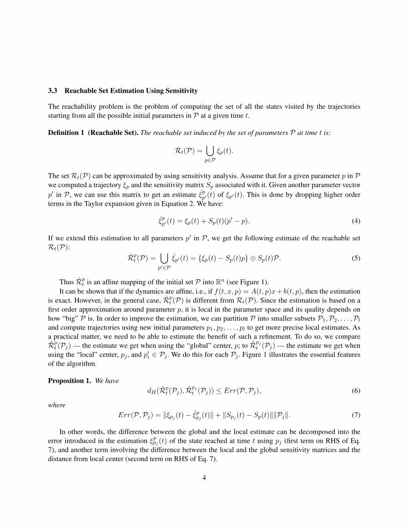
3.3 Reachable Set Estimation Using Sensitivity

The reachability problem is the problem of computing the set of all the states visited by the trajectoriesstarting from all the possible initial parameters in P at a given time t.

Definition 1 (Reachable Set). The reachable set induced by the set of parameters P at time t is:

Rt(P) =⋃p∈P

ξp(t).

The set Rt(P) can be approximated by using sensitivity analysis. Assume that for a given parameter p in Pwe computed a trajectory ξp and the sensitivity matrix Sp associated with it. Given another parameter vectorp′ in P , we can use this matrix to get an estimate ξp

p′(t) of ξp′(t). This is done by dropping higher orderterms in the Taylor expansion given in Equation 2. We have:

ξpp′(t) = ξp(t) + Sp(t)(p′ − p). (4)

If we extend this estimation to all parameters p′ in P , we get the following estimate of the reachable setRt(P):

Rpt (P) =

⋃p′∈P

ξp′(t) = {ξp(t)− Sp(t)p} ⊕ Sp(t)P. (5)

Thus Rpt is an affine mapping of the initial set P into Rn (see Figure 1).

It can be shown that if the dynamics are affine, i.e., if f(t, x, p) = A(t, p)x+ b(t, p), then the estimationis exact. However, in the general case, Rp

t (P) is different from Rt(P). Since the estimation is based on afirst order approximation around parameter p, it is local in the parameter space and its quality depends onhow “big” P is. In order to improve the estimation, we can partition P into smaller subsets P1,P2, . . . ,Pl

and compute trajectories using new initial parameters p1, p2, . . . , pl to get more precise local estimates. Asa practical matter, we need to be able to estimate the benefit of such a refinement. To do so, we compareRp

t (Pj) — the estimate we get when using the “global” center, p; to Rpj

t (Pj) — the estimate we get whenusing the “local” center, pj , and p′i ∈ Pj . We do this for each Pj . Figure 1 illustrates the essential featuresof the algorithm.

Proposition 1. We havedH(Rp

t (Pj), Rpj

t (Pj)) ≤ Err(P,Pj), (6)

whereErr(P,Pj) = ‖ξpj (t)− ξp

pj(t)‖+ ‖Spj (t)− Sp(t)‖‖Pj‖. (7)

In other words, the difference between the global and the local estimate can be decomposed into theerror introduced in the estimation ξp

pj (t) of the state reached at time t using pj (first term on RHS of Eq.7), and another term involving the difference between the local and the global sensitivity matrices and thedistance from local center (second term on RHS of Eq. 7).

4

Fig. 1. Comparison between a “global” and a “local” estimate of the reachable set. The large square on the left hand side represent aregion of parameter space, P . The oval-shaped region on the right hand side corresponds to the true reachable set, Rt(P), inducedby parameters P at time t. The large parallelogram on the right hand side corresponds to the estimated reachable set, Rp

t (P), usinga sensitivity analysis based on trajectory labeled ξp which starts at point p ∈ P . The point labeled ξp

pj, for example, is an estimate

of where a trajectory starting at point pj would reach at time t. If we partition P and consider some particular partition, Pj , wecan then compare the estimated reachable sets Rp

t (Pj) and Rpjt (Pj), which correspond to the small light-gray and small dark

gray parallelograms, respectively. We continue to refine until the distance between Rpt (Pj) and Rpj

t (Pj) (Eq. 7) falls below someuser-specified tolerance.

Proof. let y be in Rpt (Pj). There exists py in Pj such that y = ξp

py(t). We need to compare

ξppy

(t) = ξp(t) + Sp(t)(py − p) (8)

withξpjpy(t) = ξpj (t) + Spj (t)(py − pj). (9)

By introducingξppj

(t) = ξp(t) + Sp(t)(pj − p) (10)

and after some algebraic manipulations of (8), (9), and (10), we get

ξppy

(t)− ξpjpy(t) = ξpj (t)− ξp

pj(t) + (Spj (t)− Sp(t))(py − pj)

≤ ‖ξpj (t)− ξppj

(t)‖+ ‖Spj (t)− Sp(t)‖‖Pj‖ = Err(P,Pj). (11)

Let x = ξpjpy(t) which is in Rpj

t (Pj), then it can be shown that ‖y − x‖ ≤ Err(P,Pj) and sod(y, Rpj

t (Pj)) ≤ Err(P,Pj). This is true for any y ∈ Pj , thus

supy∈Rp

t (Pj)

d(y, Rpj

t (Pj)) ≤ Err(P,Pj).

Similarly, we can show thatsup

x∈Rpjt (Pj)

d(x, Rpt (Pj)) ≤ Err(P,Pj)

which proves the result. ut

5

The quantity Err(P,Pj) can be easily computed from trajectories ξp and ξpj , their corresponding sen-sitivity matrices, and ‖Pj‖. It has the following properties:

– If the dynamics is affine, then Err(P,Pj) = 0. Indeed, in this case, we have ξppj = ξpj so the first term

vanishes and Sp = Spj so the second term vanishes as well;– If limit ‖P‖ is 0, then limit Err(P,Pj) is also 0. Indeed, as ‖P‖ decreases, so does ‖p− pj‖, and thus‖ξpj (t)− ξp

pj (t)‖ and ‖Pj‖, since Pj is a subset of P . We can show that the convergence is quadratic.

The computation of reachable sets at a given time t can be extended to time intervals. Assume that T isa time interval of the form T = [t0, tf ]. The set reachable from P during T is RT (P) = ∪t∈TRt(P). Itcan be approximated by simple interpolation between Rt0(P) and Rtf (P). Of course, it may be necessaryto subdivide T into smaller intervals to improve the precision of the interpolation. A reasonable choice forthis subdivision is to use the time steps taken by the numerical solver to compute the solution of the ODEand the sensitivity matrices.

3.4 Parameter Synthesis Algorithm

In this section, we state a parameter synthesis problem and propose an algorithm that provides an approxi-mate solution. Let F be a set of ”bad” states. Our goal is to partition the set P into safe and bad parameters.That is, we want to partition the parameters into those that induce trajectories that intersect F during sometime interval T , and those that do not.

Definition 2. A solution of the parameter synthesis problem (Sys = (f,P),F , T ) where F is a set statesand T a subset of R≥0, is a partitionPbad∪Psaf ofP such that for all p ∈ Pbad (resp. p ∈ Psaf), ξp(t)∩F 6= ∅(resp. ξp(t) ∩ F = ∅) for all t ∈ T . An approximate solution is a partition P = Psaf ∪ Punc ∪ Pbad wherePsaf and Pbad are defined as before and Punc (i.e., uncertain) may contain both safe and bad parameters.

Exact solutions cannot be obtained in general, but we can try to compute an approximate solution withthe uncertain subset being as small as possible. The idea is to iteratively refine P and to classify the subsetsinto the three categories. A subset Pj qualifies as safe (resp. bad) if:

1. Rpj

T (Pj) is a reliable estimation of RT (Pj) based on the Err function;2. Rpj

T (Pj) does not (resp. does) intersect with F .

To guarantee that the process ends, we need to ensure that each refinement introduces only subsets thatare strictly smaller than the refined set.

Definition 3 (Refining Partition). A refining partition of a set P is a finite set of sets {P1, P2, . . . ,Pl}such that

– P =l⋃

j=1

Pj;

– There exists γ < 1 such that maxj∈{1,...,l}

‖Pj‖ ≤ γ‖P‖.

6

Algorithm 1 Parameter Synthesis Algorithmprocedure SAFE(P , F , t, δp, Tol)

Psaf = Pbad = ∅, Punc = {P}repeat

Pick and remove Q from Punc and let q ∈ Qfor each (qj ,Qj) ∈ ρ(Q) do

if Err(Q,Qj) ≤ Tol then . Reach set estimation is reliableif Rq

T (Qj) ∩ F = ∅ then . Reach set away from FPsaf = Psaf ∪ Qj

else if RqT (Qj) ⊂ F then . Reach set inside F

Pbad = Pbad ∪ Qj

elsePunc = Punc ∪ {(qj ,Qj)} . Some intersection with the bad set

end ifelse

Punc = Punc ∪ {(qj ,Qj)} . Reach set estimation not enough preciseend if

end foruntil Punc = ∅ or maxPj∈Punc ‖Pj‖ ≤ δpreturn Psaf, Punc, Pbad

end procedure

Let ρ be a function that maps a set to one of its refining partitions. Our algorithm stops whenever theuncertain partition is empty, or it contains only subsets with a diameter smaller than some user-specifiedvalue, δp. The complete algorithm is given by Algorithm 1 below.

The algorithm has been implemented within the Matlab toolbox Breach [11], which combines Matlabroutines to manipulate partitions with the CVODES numerical solver, which can efficiently compute ODEssolutions with sensitivity matrices.

It uses rectangular partitions of the form

P(p, ε) = {p′ : p− ε ≤ p′ ≤ p + ε}

The refinement operator ρ is such that

ρ(P(p, ε)) = {P(p1, ε1),P(p2, ε2), . . . ,P(pl, εl)},

with εk = ε/2 and pk = p + (± ε12 ,± ε2

2 , . . . ,± εn2 ). This opera-

tion is illustrated in the Figure on the right.

4 Application to Models of Acute Inflammation

We applied our method to two models of the acute inflammatory response to infection. The first is the 4-equation, 22-parameter model presented in [26], and the second is the 17-equation, 79-parameter model

7

presented in [20]. The primary difference between these models is one of detail, and the first model can bethought of as a reduced dimensional version of the second.

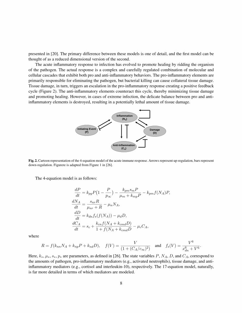
The acute inflammatory response to infection has evolved to promote healing by ridding the organismof the pathogen. The actual response is a complex and carefully regulated combination of molecular andcellular cascades that exhibit both pro and anti-inflammatory behaviors. The pro-inflammatory elements areprimarily responsible for eliminating the pathogen, but bacterial killing can cause collateral tissue damage.Tissue damage, in turn, triggers an escalation in the pro-inflammatory response creating a positive feedbackcycle (Figure 2). The anti-inflammatory elements counteract this cycle, thereby minimizing tissue damageand promoting healing. However, in cases of extreme infection, the delicate balance between pro and anti-inflammatory elements is destroyed, resulting in a potentially lethal amount of tissue damage.

Initiating Event(P)

Inflammation(NA)

Anti-Inflammation(CA)

Damage(D)

Fig. 2. Cartoon representation of the 4-equation model of the acute immune response. Arrows represent up-regulation, bars representdown-regulation. Figurere is adapted from Figure 1 in [26].

The 4-equation model is as follows:

dP

dt= kpgP

(1− P

p∞

)− kpmsmP

µm + kmpP− kpmf(NA)P,

dNA

dt=

snrR

µnr + R− µnNA,

dD

dt= kdnfs(f(NA))− µdD,

dCA

dt= sc +

kcnf(NA + kcmdD)1 + f(NA + kcmdD

− µcCA,

where

R = f(knnNA + knpP + kndD), f(V ) =V

(1 + (CA/c∞)2)and fs(V ) =

V 6

x6dn + V 6

.

Here, k∗, µ∗, s∗, p∗ are parameters, as defined in [26]. The state variables P , NA, D, and CA, correspond tothe amounts of pathogen, pro-inflammatory mediators (e.g., activated neutrophils), tissue damage, and anti-inflammatory mediators (e.g., cortisol and interleukin-10), respectively. The 17-equation model, naturally,is far more detailed in terms of which mediators are modeled.

8

0 100 200 300 400 500−10

0

10

p

0 100 200 300 400 5000

10

20

d

0 100 200 300 400 5000

1

2

na

0 100 200 300 400 5000

0.5

1

ca

time

0 50 100 150 200 250 300 350 400 450 5000

2

4

d

0 50 100 150 200 250 300 350 400 450 500−10

0

10

p

0 50 100 150 200 250 300 350 400 450 5000

1

2

cai

0 50 100 150 200 250 300 350 400 450 5000

1

2

il6

0 50 100 150 200 250 300 350 400 450 5000

5

n

time

(A) (B)

Fig. 3. (A) Examples trace from the 4-equation model. There are three different traces corresponding to septic death, aseptic deathand health. (B) Example traces from the 17-equation model; 5 of the 17 variables are shown. There are also three traces, illustratingthe richer dynamics of the model. Two traces corresponds to aseptic death and the third to health with a periodic small resurgenceof the pathogen. Time is measured in hours.

In each model, there are 3 clinically relevant outcomes: (i) a return to health, (ii) aseptic death, and(iii) septic death. Death is defined as a sustained amount of tissue damage (D) above a specified thresholdvalue and constitutes the undesirable or “bad” outcome we wish to avoid. Aseptic and septic death aredistinguished by whether the pathogen (P ) is cleared below a specified threshold value. Let Falive (resp.Fdead) refer to the set of states such that D is below (resp. above) some threshold Ddeath, and let Fseptic

(resp. Faseptic) refer to the set of states such that P is above (resp. below) some threshold Pseptic. Wecan now define three sets of states corresponding to the three clinically relevant outcomes as follows: (i)Health = Falive∩Faseptic; (ii) Aseptic death = Fdead∩Faseptic; and (iii) Septic death = Fdead∩Fseptic.In Figure 3 we present sample traces for both the 4 and 17 equation models.

4.1 Experiments

We performed several experiments. In the first experiment, we validated our method by reproducing resultspreviously obtained in [26] using bifurcation analysis. Figure 4-A contrasts the initial amount of pathogen,P0, and the initial amount of anti-inflammatory mediators, CA0. The growth rate of pathogen, kpg, wasset to 0.3 and other parameters to their nominal values. The region Fdeath given by D ≥ 5 was used in ouralgorithm and we checked the intersection with reachable set at time 300 hours. Crosses correspond to initialvalues leading to death while circles lead to an healthy outcome. We can see that the resulting partition isquantitatively consistent with Figure 8 in [26]. In our second experiment, we varied growth rate of pathogen,kpg, and NA. Figure 4-(B) shows that there are three distinct regions in the kpg-NA plane, corresponding tothe three clinical outcomes.

9

0 0.2 0.4 0.6 0.8 1 1.2 1.4 1.6 1.8 20

0.1

0.2

0.3

0.4

0.5

0.6

0.7

0.8

p

ca

0 0.02 0.04 0.06 0.08 0.1 0.12 0.14 0.160.1

0.2

0.3

0.4

0.5

0.6

0.7

0.8

na

kpg

(A) (B)

Fig. 4. Results obtained for the 4-equation model. Figure (A) reproduces results presented in Figure 8 of [26] with kpg = 0.3,which was obtained using classical bifurcation analysis. Circles are parameter values leading to Health while crosses representvalues leading to Death. Figure (B) illustrates how a pair of parameters (NA and kpg) can be partitioned into the three possibleoutcomes. Circles alone lead to Health, crosses and circles lead to Aseptic Death and crosses alone lead to Septic Death. Theseparation between regions is induced from small uncertain regions computed by the algorithm.

(A) (B)

Fig. 5. Results for the 17-equation model. Figure (A) illustrates the kpg-NA plane, partitioned into regions leading to death (hereaseptic death, represented by crosses) and regions leading to health (represented by circles). Figure (B) illustrates the kpg-CAI

plane. Interestingly, the separation is not monotone with the growth of pathogen kpg .

10

We then performed several experimentations with the 17-equation model. Figures 5 (A) and (B) depictthe kpg-NA and kpg-CAI planes, respectively. CAI is a generic anti-inflammatory mediator. We partitionedthe region using Fdeath = D > 1.5 and checked after time 300 hours. The 17-equation model exhibitsan interesting behavior in the kpg-CAI plane. Namely, that the separation between health and death is notmonotone in the growth rate of the pathogen.

As previously mentioned, our algorithm is implemented in Matlab and uses the CVODES numericalsolver. Figures 4 (A) and (B) were generated in a few seconds, and Figures 5 (A) and (B) were generatedin about an hour on a standard laptop (Intel Dual Core 1.8GHz with 2 Gb of memory). We note that thealgorithm could easily be parallelized.

5 Discussion and Conclusions

Complex models are increasingly being used to make predictions about complex phenomena in biology andmedicine (e.g., [3, 25]). Such models can be potentially very useful in guiding early decisions regardingintervention, but it is often impossible to obtain accurate estimates for every parameter. Thus, it is importantto have tools for explicitly examining a range of possible parameters to determine whether the behavior of themodel is sensitive to those parameters that are poorly estimated. Performing this task for nonlinear modelsis especially challenging. We have presented an algorithm for solving the parameter synthesis problem fornonlinear dynamical models and applied it on two models of acute inflammation from the literature. Thelarger of the two has 17 equations and 79 parameters, demonstrating the scalability of our approach.

Our approach has several limitations. First, our refinement process implies that the number of partitionsincreases exponentially with the number of varying parameters. Thus, in practice, some variables must beheld fixed while analyzing the behavior of the model. On the other hand, the number of state variables isnot a limiting factor, as illustrated in our experiments on the 17-equation model. Second, our method re-lies on numerical simulations. Numerical methods are fundamentally limited in the context of verificationsince numerical image computation is not semi-decidable for nonlinear differential equations [23]. More-over, there are no known methods capable of providing provable bounds on numerical errors for generalnonlinear differential equations. Thus, we cannot claim to provide formal guarantees on the correctness ofthe results computed by our method. However asymptotic guarantees exist, meaning that results can alwaysbe improved by decreasing tolerance factors in the numerical computations. A nice feature of our approachis that it enables one to obtain qualitative results using a few simulations (e.g. a coarse partition betweenregions leading to qualitatively different behaviors). These qualitative results can then be made as precise asdesired by focusing on smaller partitions.

There are several areas for future research. Our first order error control mechanism can be improvedto make the refinements more efficient and more adaptive when nonlinear (i.e. higher order) behaviorsdominate any linear dependance on parameter variations. We are also interested in developing techniques forverifying properties that are more complex than the reachability predicates we considered in this paper. Forinstance, temporal properties could easily be introduced in our framework. The extended system could thenbe used, for example, verify the possible outcomes associated with a particular medical intervention. Finally,we believe that the method could easily be used in the context of personalized medicine. In particular, givenindividual or longitudinal measurements from a specific patient, we could define a reachable set, Fobs, that

11

includes these observations (possibly convolved with a model of the measurement errors). We could then useour method to identify the set of parameters that are consistent with the observations. The refined parameterscan then be used to make patient-specific predictions.

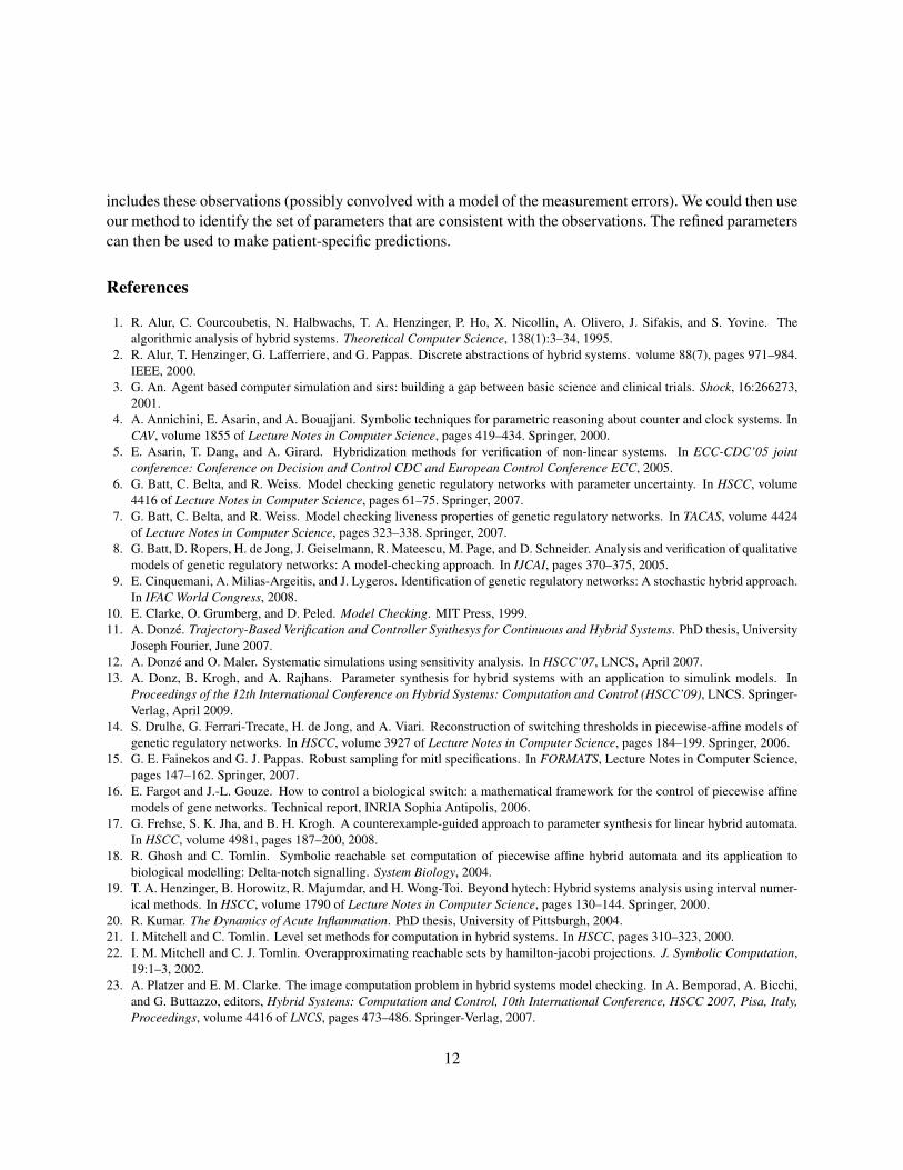
References

1. R. Alur, C. Courcoubetis, N. Halbwachs, T. A. Henzinger, P. Ho, X. Nicollin, A. Olivero, J. Sifakis, and S. Yovine. Thealgorithmic analysis of hybrid systems. Theoretical Computer Science, 138(1):3–34, 1995.

2. R. Alur, T. Henzinger, G. Lafferriere, and G. Pappas. Discrete abstractions of hybrid systems. volume 88(7), pages 971–984.IEEE, 2000.

3. G. An. Agent based computer simulation and sirs: building a gap between basic science and clinical trials. Shock, 16:266273,2001.

4. A. Annichini, E. Asarin, and A. Bouajjani. Symbolic techniques for parametric reasoning about counter and clock systems. InCAV, volume 1855 of Lecture Notes in Computer Science, pages 419–434. Springer, 2000.

5. E. Asarin, T. Dang, and A. Girard. Hybridization methods for verification of non-linear systems. In ECC-CDC’05 jointconference: Conference on Decision and Control CDC and European Control Conference ECC, 2005.

6. G. Batt, C. Belta, and R. Weiss. Model checking genetic regulatory networks with parameter uncertainty. In HSCC, volume4416 of Lecture Notes in Computer Science, pages 61–75. Springer, 2007.

7. G. Batt, C. Belta, and R. Weiss. Model checking liveness properties of genetic regulatory networks. In TACAS, volume 4424of Lecture Notes in Computer Science, pages 323–338. Springer, 2007.

8. G. Batt, D. Ropers, H. de Jong, J. Geiselmann, R. Mateescu, M. Page, and D. Schneider. Analysis and verification of qualitativemodels of genetic regulatory networks: A model-checking approach. In IJCAI, pages 370–375, 2005.

9. E. Cinquemani, A. Milias-Argeitis, and J. Lygeros. Identification of genetic regulatory networks: A stochastic hybrid approach.In IFAC World Congress, 2008.

10. E. Clarke, O. Grumberg, and D. Peled. Model Checking. MIT Press, 1999.11. A. Donze. Trajectory-Based Verification and Controller Synthesys for Continuous and Hybrid Systems. PhD thesis, University

Joseph Fourier, June 2007.12. A. Donze and O. Maler. Systematic simulations using sensitivity analysis. In HSCC’07, LNCS, April 2007.13. A. Donz, B. Krogh, and A. Rajhans. Parameter synthesis for hybrid systems with an application to simulink models. In

Proceedings of the 12th International Conference on Hybrid Systems: Computation and Control (HSCC’09), LNCS. Springer-Verlag, April 2009.

14. S. Drulhe, G. Ferrari-Trecate, H. de Jong, and A. Viari. Reconstruction of switching thresholds in piecewise-affine models ofgenetic regulatory networks. In HSCC, volume 3927 of Lecture Notes in Computer Science, pages 184–199. Springer, 2006.

15. G. E. Fainekos and G. J. Pappas. Robust sampling for mitl specifications. In FORMATS, Lecture Notes in Computer Science,pages 147–162. Springer, 2007.

16. E. Fargot and J.-L. Gouze. How to control a biological switch: a mathematical framework for the control of piecewise affinemodels of gene networks. Technical report, INRIA Sophia Antipolis, 2006.

17. G. Frehse, S. K. Jha, and B. H. Krogh. A counterexample-guided approach to parameter synthesis for linear hybrid automata.In HSCC, volume 4981, pages 187–200, 2008.

18. R. Ghosh and C. Tomlin. Symbolic reachable set computation of piecewise affine hybrid automata and its application tobiological modelling: Delta-notch signalling. System Biology, 2004.

19. T. A. Henzinger, B. Horowitz, R. Majumdar, and H. Wong-Toi. Beyond hytech: Hybrid systems analysis using interval numer-ical methods. In HSCC, volume 1790 of Lecture Notes in Computer Science, pages 130–144. Springer, 2000.

20. R. Kumar. The Dynamics of Acute Inflammation. PhD thesis, University of Pittsburgh, 2004.21. I. Mitchell and C. Tomlin. Level set methods for computation in hybrid systems. In HSCC, pages 310–323, 2000.22. I. M. Mitchell and C. J. Tomlin. Overapproximating reachable sets by hamilton-jacobi projections. J. Symbolic Computation,

19:1–3, 2002.23. A. Platzer and E. M. Clarke. The image computation problem in hybrid systems model checking. In A. Bemporad, A. Bicchi,

and G. Buttazzo, editors, Hybrid Systems: Computation and Control, 10th International Conference, HSCC 2007, Pisa, Italy,Proceedings, volume 4416 of LNCS, pages 473–486. Springer-Verlag, 2007.

12

24. A. Pnueli. The temporal logic of programs. In Proc. 18th Annual Symposium on Foundations of Computer Science (FOCS),pages 46–57, 1977.

25. D. Polidori and J. Trimmer. Bringing advanced therapies to marker faster: a role for bio-simulation? Diabetes Voice, 48(2):28–30, 2003.

26. A. Reynolds, J. Rubin, G. Clermont, J. Day, Y. Vodovotz, and B. Ermentrout. A reduced mathematical model of the acuteinflammatory response: I. derivation of model and analysis of anti-inflammation. J Theor Biol, 242(1):220–236, 2006.

27. R. Serban and A. C. Hindmarsh. Cvodes: the sensitivity-enabled ode solver in sundials. In Proceedings of IDETC/CIE 2005,Long Beach, CA., Sept. 2005.

28. O. Stursberg and B. H. Krogh. Efficient representation and computation of reachable sets for hybrid systems. In HSCC, pages482–497, 2003.

13