Reduction of dimension for nonlinear dynamical systems · Reduction of dimension for nonlinear dynamical systems ... elimination ·Nonlinear dynamics ·Chaotic ... Reduction of dimension

Nonlinear Dyn (2017) 88:715–734DOI 10.1007/s11071-016-3272-5

ORIGINAL PAPER

Reduction of dimension for nonlinear dynamical systems

Heather A. Harrington · Robert A. Van Gorder

Received: 24 August 2015 / Accepted: 7 December 2016 / Published online: 19 December 2016© The Author(s) 2016. This article is published with open access at Springerlink.com

Abstract We consider reduction of dimension fornonlinear dynamical systems. We demonstrate that insome cases, one can reduce a nonlinear system of equa-tions into a single equation for one of the state vari-ables, and this can be useful for computing the solu-tion when using a variety of analytical approaches. Inthe case where this reduction is possible, we employdifferential elimination to obtain the reduced system.While analytical, the approach is algorithmic and isimplemented in symbolic software such asMAPLE orSageMath. In other cases, the reduction cannot beperformed strictly in terms of differential operators,and one obtains integro-differential operators, whichmay still be useful. In either case, one can use thereduced equation to both approximate solutions forthe state variables and perform chaos diagnostics moreefficiently than could be done for the original higher-dimensional system, as well as to construct Lyapunovfunctions which help in the large-time study of thestate variables. A number of chaotic and hyperchaoticdynamical systems are used as examples in order tomotivate the approach.

H. A. Harrington · R. A. Van Gorder (B)Mathematical Institute, University of Oxford, AndrewWiles Building, Radcliffe Observatory Quarter, WoodstockRoad, Oxford OX2 6GG, UKe-mail: [email protected]

H. A. Harringtone-mail: [email protected]

Keywords Reduction of dimension · Differentialelimination · Nonlinear dynamics · Chaotic attractors ·Computation of chaos

1 Introduction

Nonlinear dynamical systems are ubiquitous in math-ematics, engineering, and the sciences, with manyreal-world phenomenon governed by such nonlinearprocesses. In particular, nonequilibrium and chaoticdynamics are a continuing area of active researchfor applied mathematicians, as approximating suchdynamics accurately and efficiently can be quite chal-lenging. In the present paper, we shall consider reduc-tion of dimension1 for nonlinear dynamical systems.This approach has previously been employed in theliterature in order to enable the construction of Lya-punov functions [1] and equilibrium dynamics [2], aswell as to allow one tomore easily approximate chaoticattractors analytically [3–5]. One method for reductionof dimension is differential elimination, in which onealgorithmically reduces the nonlinear dynamical sys-tem into a single ordinary differential equation (ODE)for one of the state variables. However, this is possible

1 We refer to the method as reduction of dimension, rather thanreduction of order, as in many cases the differential order isunchanged. Rather, we are eliminating scalar functions, andhence, the number of unknown scalar functions is reduced. Thismethod could also be referred to as reduction of scalar dimen-sion.

123

http://crossmark.crossref.org/dialog/?doi=10.1007/s11071-016-3272-5&domain=pdf

716 H. A. Harrington, R. A. Van Gorder

only when the system reduces to an ODE; if the reduc-tion is instead to an integro-differential equation, theprocess is not algorithmic and specific cases must behandled with more individual care. Our focus shall beon dynamical systems giving chaotic dynamics, but theapproach can certainly be applied for non-chaotic ODEsystems. We give an overview of reduction of dimen-sion, after which we demonstrate in several ways whyone might wish to apply this technique.

With the wide range of numerical methods avail-able for solving nonlinear first-order ODE systems ofhigh order, one may wonder why it might be advanta-geous to convert such systems into a single higher-orderODE. We shall mention several situations in which thedifferential elimination, and more generally reductionof dimension, may prove useful. We then outline thepaper.

Often times, if one is trying to approximate the solu-tion to a nonlinear system through some sort of ana-lytical approximation, via series, perturbation, or morecomplicated approaches, one quickly finds that the cou-pled equations require balancing many terms comingfrom the expansion for each of the state variables. Inthe case of a single state variable governed by a higher-order ODE, one needs only track terms in a singleasymptotic expansion. This approach has been appliedwhen using Taylor series, approximate Fourier series,and asymptotic expansions in other types of basis func-tions to the solution of a system of nonlinear ODE. Inhybrid analytic–numeric methods, such as the homo-topy analysismethod [6], such reductions of a system toa single equation also simplify the optimization prob-lem which is solved to obtain the error-minimizingsolution (see, for instance, [2], where the presentapproach is used in such a capacity). Therefore, thereduction of dimension can greatly reduce the complex-ity of analytical calculations under several frameworks.

Contraction maps or Lyapunov functions are use-ful tools for discussing the convergence of solutionsto nonlinear dynamical systems to large-time steadyor quasi-steady dynamics. In situations where contrac-tion maps or Lyapunov functions are known for a givendynamical system, the state variable governed by a sin-gle higher-order ODE necessarily results in a contrac-tionmap in the single state variable. However, as is wellknown to those studying stability of nonlinear systems,it is not often easy to obtain contraction maps for com-plicated systems.Aswe shall showhere, it is possible touse the reduction of a system to a single higher-order

ODE in order to construct a contraction map for thestate variable governed by the aforementioned higher-order ODE. The existence of such a map can then beused to deduce the large-time dynamics of the statevariable, as well as for the other state variables in theoriginal system. One example of this is given in [1],and other examples are provided in Sect. 5.

Related to both the topic of analytical approx-imations and Lyapunov functions would be long-time dynamics and equilibrium behavior of nonlineardynamical systems. Indeed, in order to study the equi-librium structure of a high-order system of ODEs, onemust solve a coupled system of nonlinear algebraicequations in order to recover the fixed points for thestate variables. First reducing the system to a singleODE allows one to obtain a single nonlinear algebraicequation for the fixed point of a single state variable,which can then be used to recover the fixed points ofthe other state variables. Therefore, when such a reduc-tion to a single ODE is possible, the need to solve anonlinear algebraic system for all of the fixed pointssimultaneously is eliminated, resulting in what is oftena far less computationally demanding problem.

Another topic is great recent interest in nonlinearscience has been both the synchronization of chaos[7] and the control of chaos. In situations where oneis interested in mitigating the possibility of emergentchaos, one can couple a chaotic system to variouscontrol terms, or indeed to additional dynamical sys-tems, which may lend a degree to stability. Under suchapproaches, one often increases the complexity or eventhe dimension of the dynamical system being solved.As such, methods to reduce the dimension of such sys-tems could improve compatibility. Furthermore, sincethe control of chaos is often linked to a control termwhich itself is determined by a Lyapunov function, theconstruction of contraction maps through the reductionapproach outlined here could be of great use.

As stated before [8], the competitive modes anal-ysis gives an interesting link between the geometryof phase space possibly yielding chaotic trajectories(recall that the competitive modes requirements appearto be a necessary, albeit not sufficient, condition forchaos [9–14]). Conversely, the differential eliminationmay cast light into the geometry of solutions in thespace of derivations. Since this result of the differen-tial elimination is a single higher-order ODE, and sinceany chaos emergent from the nonlinear system shouldbe encoded in the single higher-order ODE, the differ-

123

Reduction of dimension for nonlinear dynamical systems 717

ential algebraic structure of such equations may castlight into practical geometric tools by which one maystudy systems in which chaos is observed. In particu-lar, through this reduction approach, the calculation ofmode frequencies in the standard competitive modesanalysis becomes much simpler.

This paper is outlined as follows. In Sect. 2, weprovide an algorithmic approach, to differential elim-ination for nonlinear dynamical systems based upondifferential algebra. First laying out the general the-ory, we then give specific MAPLE code for perform-ing the differential elimination in a systematic man-ner. The algorithmic approach is useful in the casewhere the dynamical system can be reduced to a sin-gle ODE in terms of only one of the state variables. InSect. 3, we implement the approach in order to reducea variety of chaotic and hyperchaotic systems, find-ing that the form of the nonlinearity in the dynamicalsystem will strongly influence the reducibility proper-ties.2 However, in cases where the dynamical systemis not reducible using differential elimination, one maystill obtain more complicated reductions, for instancein terms of integrals, resulting in more complicatedintegro-differential equations for the reduced state vari-able. The possible results are illustrated through con-crete examples for the Rössler system (which is com-pletely reducible), theLorenz system (which is partiallyreducible—that is, reducible in some but not all statevariables), and the Qi–Chen–Du–Chen–Yuan (whichis irreducible under differential elimination, but whichcan be reduced to an integro-differential equation). Wegive summarizing observations regarding the reducibil-ity of dynamical systems in Sect. 4.

The remainder of the paper is devoted to applica-tions of reduction of dimension for dynamical systems.In Sect. 5, we demonstrate that reduction of dimen-sion can be useful for obtaining contraction maps andLyapunov functions, which in turn may be used todetermine asymptotic stability of dynamical systemsand also to control chaos in such systems. In Sect. 6,we demonstrate that reduction of dimension can beused to simplify calculations involved in certain tech-niques for studying the solutions of nonlinear dynami-cal systems. Indeed, when applicable, we find that the

2 Note that we also provide a long list of systems with nondi-mensional parameters in the Appendices, which could prove auseful resource for those wishing to have a unified list of chaoticand hyperchaotic systems and references for each system.

approach greatly reduces the number of nonlinear alge-braic equations required to be solvedwhen constructingtrajectories in state space via undetermined coefficientmethods by a factor of 1/n, where n is the dimensionof the dynamical system, meaning that the number ofequations needing to be solved will not increase withthe size of the system. Furthermore, when applying thecompetitivemodes analysis (which is a type of diagnos-tic criteria for finding chaotic trajectories in nonlineardynamical systems), we find that only one binary com-parison is needed if one first reduces the dimension ofthe dynamical system so that there is a single equationfor one state variable. In contrast, there are normally oforder 2n−1 comparisons needed for an n-dimensionaldynamical system. In Sect. 7, we provide a discussionand possible avenues for future work.

2 Algebraic approach to differential elimination

Systems of differential equations are ubiquitous andwidely studied. Ritt [15] and Kolchin [16] pioneeredthe field of differential algebra, an algebraic theory forstudying solutions of ordinary and partial differentialequations. We are particularly interested in differentialelimination, an algorithmic subtheory that can simplifysystems of parameterized algebraic differential equa-tions. This permits one to reduce the dimension of adynamical system so that one is left with a single ODEin the state variable.

2.1 Algebra preliminaries

Here we briefly review concepts from algebra and dif-ferential algebra. For reference books in differentialalgebra, see [15,16]. If I is a subset of a ring R, then(I ) is the (algebraic) ideal generated by I . Let I be anideal of R. Then

√I denotes the radical of I . A deriva-

tion over a ring R is a map R �→ R which satisfies (wewrite a is the derivative of a), for every a, b ∈ R,

˙(a + b) = a+ b and ˙(a b) = (a)b+ a(b). The field ofdifferential algebra is based on the concept of a differ-ential ring (resp. field), which is a ring (resp. field) Rendowed with a set of derivations that commutes pair-wise. A differential ideal [I ] of a differential ring R isan ideal of R stable under the action of derivation.

Differential algebra is more similar to commutativealgebra than analysis. In commutative algebra, Buch-

123


berger solved themembership problem (tests whether agiven polynomial is contained in a given ideal) throughthe theory ofGröbner bases [25]. Fromalgebraic geom-etry, we know the set of polynomials which vanish overthe solutions of a given polynomial system form anideal and even a radical ideal [26]. In the case of dif-ferential equations, the set of differential polynomialswhich vanish over the analytic solutions of a given sys-tem of differential polynomial equations form a differ-ential ideal and even a radical differential ideal [15].Ritt solved the theoretical problem (of membership forradical differential ideals) and developed algorithmictools to solve systems of polynomial ODE and PDEs;however, Ritt’s algorithm requires factorization.

Due to the complexity of factorization, Boulier andco-authors avoided it by developing the Rosenfeld–Gröbner algorithm, based on the work of Seidenbergand Rosenfeld, and incorporating Gröbner bases [19,20,22]. Since then, the algorithm has been improvedboth theoretically and practically [17,18,21] and it nolonger requires Gröbner bases. It is available in theDifferentialAlgebra package in MAPLE [17]and SageMath as an interface for the BLAD and BMIlibraries [27,28].

Algorithmically, differential elimination involvesmanipulation of finite subsets of a differential polyno-mial ring R = K {U } where K is the differential fieldof coefficients (i.e., K = Q), and U is a finite set ofdependent variables. The elements of R are differen-tial polynomials, which are polynomials built over theinfinite set of all derivativesΘU , of the dependent vari-ables. Considering a system Σ of polynomial differen-tial equations, here, we consider the Lorenz system ofthree ordinary differential equations:

x1 = a(x2 − x1) ,

x2 = x1(b − x3) − x2 ,

x3 = x1x2 − cx3 .

(1)

The Lorenz system can be rewritten as:

Σ =

⎧⎪⎨

⎪⎩

−x1 + a(x2 − x3) = 0 ,

−x2 + x1(b − x3) − x2 = 0 ,

−x3 + x1x2 − cx3 = 0 .

(2)

The Rosenfeld–Gröbner algorithm takes as an inputa differential system Σ and a ranking. A ranking >

is any total ordering over the set ΘU of all deriva-

tives of the elements of U which satisfies the follow-ing axioms: a < a and a < b ⇒ a < b for alla, b ∈ ΘU . The Rosenfeld–Gröbner algorithm trans-forms Σ into finitely many systems called regular dif-ferential systems, which reduces differential problemsto purely algebraic ones that are triangular. The nextstep is purely algebraic and transforms the regular dif-ferential system into finitely many characteristic pre-sentations,C1, . . .Cr . Rosenfeld–Gröbner outputs thisfinite family C1, . . .Cr of finite subsets of K {U } \ K ,where eachCi defines a differential ideal [Ci ]. The rad-ical

√[Σ] of the differential ideal generated by Σ isthe intersection presented by characteristic sets:

√[Σ] = [Ci ] ∩ · · · ∩ [Cr ].

Note differential ideals [Ci ] do not need to be prime;however by Lazard’s lemma, they are necessarily rad-ical. Differential algebra elimination has proven use-ful for parameter estimation, identifiability, and modelreduction of biological and chemical systems [23,24].

2.2 Computational method

We demonstrate reduction in dimension via differentialelimination algorithm RosenfeldGroebner in theDifferentialAlgebra package implemented inMAPLE. For the sake of using a concrete example, wechoose the Lorenz system. First, we call the package:

with(DifferentialAlgebra) :

Next we input the Lorenz system:

sys := [−(diff(x1(t),t)) + a ∗ (x2(t) − x1(t)),

−(diff(x2(t),t)) + x1(t) ∗ (b − x3(t)) − x2(t),

−(diff(x3(t),t)) + x1(t) ∗ x2(t) − c ∗ x3(t)]

Next we form our differential ring, embedding therank of dependent variables in blocks and inde-pendent variables in derivations. Since we areconsideringordinarydifferential equations, derivationsare set to one ordering, time t . We remark that theDifferentialAlgebra package enables differen-tial elimination of PDEs by including additional inputsfor the derivations (e.g., derivations=[u,x,t].Note, sys is assumed to have coefficients in the fieldQ[x1, x2, x3] obtained by adjoining the independent

123


variables to the field of rationals, and symbolic param-eters a, b, c are considered arbitrary in the coefficientfield. To form the differential ring, we input:

R := DifferentialRing(blocks

= [x3,x2,x1],derivations = [t])Note that x1 stands to the rightmost place on the listwhich identifies that we are attempting to reduce thedifferential equation to only one variable, i.e., x1(t).This ranking eliminates x3 with respect to x2, andthen eliminates x2 with respect to x1. We now call theRosenfeld–Gröbner algorithm for our system and dif-ferential polynomial ring:

G := RosenfeldGroebner(sys,R)

simplify(Equations(G[1],solved))

This will return the characteristic presentation (whichshould be understood as an intersection), with the equa-tions given by the ranking, with the final equation asingle ODE for x1(t), provided that it exists and canbe computed by the algorithm. In some cases, the algo-rithmwill keep running and therefore should eventuallybe terminated by the user. For such cases, it is unlikelythat a reduction of the specified form exists. However,aswe shall consider in the next section, when the reduc-tion is to an integro-differential equation, rather than anODE, the approach will not identify the reduced equa-tion.

3 Reduction of dimension: applications

Here we apply the method of differential elimina-tion to several nonlinear dynamical systems known togive chaos, in order to see if these equations can bereduced. We first apply the algorithmic approach out-lined in Sect. 2, finding that the approach gives a com-plete reduction (all state variables can be isolated andexpressed as the solution to single uncoupled ODEs),a partial reduction (one or more, but not all, state vari-ables can be isolated and expressed as the solutionto single uncoupled ODEs), or returns no reduction(the algorithm does not complete in a fixed amountof time), in which case none of the state variables canbe expressed as a solution to a single ODE reduciblefrom the original system. For simplicity, we shall onlyconsider autonomous systems.

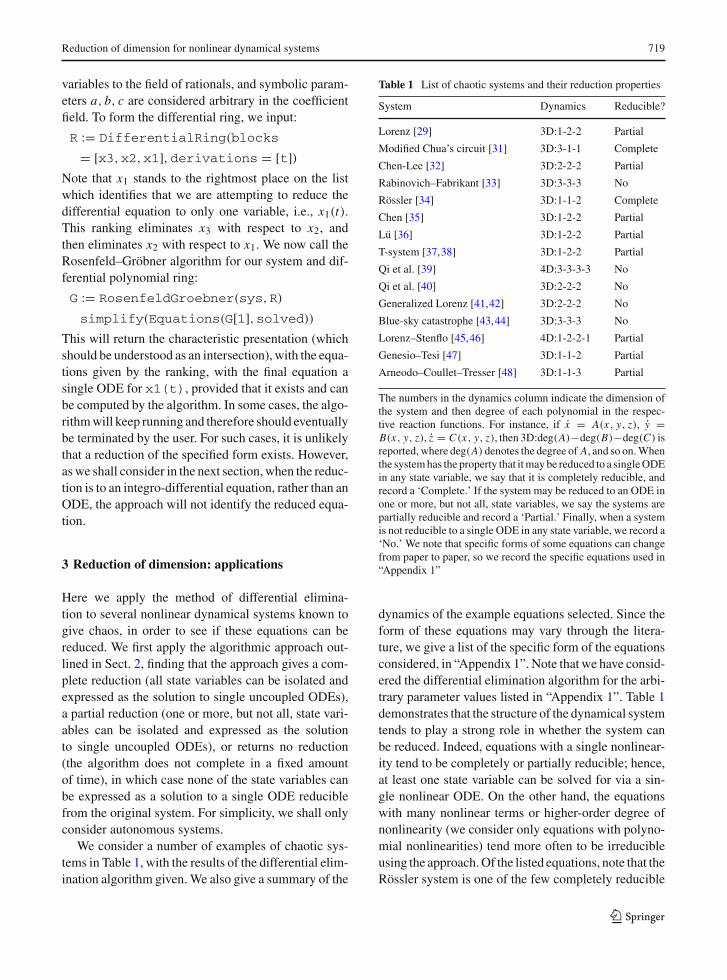
We consider a number of examples of chaotic sys-tems in Table 1, with the results of the differential elim-ination algorithm given.We also give a summary of the

Table 1 List of chaotic systems and their reduction properties

System Dynamics Reducible?

Lorenz [29] 3D:1-2-2 Partial

Modified Chua’s circuit [31] 3D:3-1-1 Complete

Chen-Lee [32] 3D:2-2-2 Partial

Rabinovich–Fabrikant [33] 3D:3-3-3 No

Rössler [34] 3D:1-1-2 Complete

Chen [35] 3D:1-2-2 Partial

Lü [36] 3D:1-2-2 Partial

T-system [37,38] 3D:1-2-2 Partial

Qi et al. [39] 4D:3-3-3-3 No

Qi et al. [40] 3D:2-2-2 No

Generalized Lorenz [41,42] 3D:2-2-2 No

Blue-sky catastrophe [43,44] 3D:3-3-3 No

Lorenz–Stenflo [45,46] 4D:1-2-2-1 Partial

Genesio–Tesi [47] 3D:1-1-2 Partial

Arneodo–Coullet–Tresser [48] 3D:1-1-3 Partial

The numbers in the dynamics column indicate the dimension ofthe system and then degree of each polynomial in the respec-tive reaction functions. For instance, if x = A(x, y, z), y =B(x, y, z), z = C(x, y, z), then 3D:deg(A)−deg(B)−deg(C) isreported, where deg(A) denotes the degree of A, and so on.Whenthe systemhas the property that itmay be reduced to a singleODEin any state variable, we say that it is completely reducible, andrecord a ‘Complete.’ If the system may be reduced to an ODE inone or more, but not all, state variables, we say the systems arepartially reducible and record a ‘Partial.’ Finally, when a systemis not reducible to a single ODE in any state variable, we record a‘No.’ We note that specific forms of some equations can changefrom paper to paper, so we record the specific equations used in“Appendix 1”

dynamics of the example equations selected. Since theform of these equations may vary through the litera-ture, we give a list of the specific form of the equationsconsidered, in “Appendix 1”. Note that we have consid-ered the differential elimination algorithm for the arbi-trary parameter values listed in “Appendix 1”. Table 1demonstrates that the structure of the dynamical systemtends to play a strong role in whether the system canbe reduced. Indeed, equations with a single nonlinear-ity tend to be completely or partially reducible; hence,at least one state variable can be solved for via a sin-gle nonlinear ODE. On the other hand, the equationswith many nonlinear terms or higher-order degree ofnonlinearity (we consider only equations with polyno-mial nonlinearities) tend more often to be irreducibleusing the approach.Of the listed equations, note that theRössler system is one of the few completely reducible

123


Table 2 List of hyperchaotic systems and their reduction prop-erties

System Dynamics Reducible?

Rössler [49] 4D:1-1-2-1 Complete

Chen [50] 4D:1-2-2-1 Partial

Lü [51] 4D:1-2-2-2 No

Modified Lü [52] 4D:2-2-2-1 No

Wang-Liu [53] 4D:1-2-2-1 Partial

Jia [54] 4D:1-2-2-2 Partial

QWWC system [55] 4D:2-2-2-2 No

The labeling is the same as given in Table 1.We note that specificforms of some equations can change from paper to paper, so werecord the specific equations used in “Appendix 2”

systems, lending validity to the belief that it is indeedoneof the simplest possible continuous-timedynamicalsystems giving chaos. Meanwhile, the commonly stud-ied Lorenz system is only partially reducible under theapproach. More complicated systems tend to be irre-ducible under the algorithm, and many of these givemore complicated dynamics such as multiple scrollattractors.

Note that the algorithm returns a ‘No’ if a reductionis not obtained within a given time interval. For caseswhere the algorithm found a reduction, the computa-tion time was fairly quick. We are therefore comfort-able in assuming that a reduction to an ODE does notexist in cases where the algorithm times out. For suchcases, the system may still admit a reduction, but notstrictly in derivatives of one of the state variables. Onesuch example would be a system which is reducibleto an integro-differential equation in one of the statevariables, but never to simply an ODE.

Wenext consider hyperchaotic systems (chaotic sys-tems giving two or more positive Lyapunov expo-nents) in Table 2. Again, we find that the more com-plicated the functional form of the nonlinearities, theless likely a system seems to be reducible. Further-more, hyperchaotic generalizations of known chaoticsystems appear to maintain their reducibility proper-ties, since often a simple additional equation is addedto make a chaotic system hyperchaotic. The hyper-chaotic Rössler system is completely reducible, as wasthe related chaotic Rössler system, again suggestingthat the chaotic and hyperchaotic Rössler systems aresome of the simplest systems which still exhibit chaosand hyperchaos, respectively.

The results indicate that completely reducible sys-tems are perhaps the simplest systems giving chaosor hyperchaos. Again, this would support the quali-tative and topological claims that the Rössler systemsare some of the simplest possible equations permittingchaos [56], as they each involve only a single quadraticnonlinearity. On the other hand, systems with strongerpolynomial nonlinearities, or systems with many non-linear terms, appear to often be irreducible under dif-ferential elimination. Note that for cases where thereduction might involve integrals, resulting in a typeof integro-differential equation, the differential elim-ination algorithm would miss such a reduction, eventhough it exists. This is due to the fact that the differen-tial elimination algorithm is working over the ring ofderivations, which does not include integrals. Indeed,since integral operators are fairly cumbersome to intro-duce compared to their differential operator counter-parts (wediscuss this later in Sect. 7), obtaining an algo-rithmic approach including integrals would be chal-lenging. Therefore, the differential elimination algo-rithm outlined in Sect. 2 appears to be a very usefultool for reducing the dimension of dynamical systems,provided that a reduction to a singleODEexists. For themore complicated models, we find the need to proceedon a case-by-case basis withmanual manipulations dueto any integration needed.

We demonstrate reduction of dimension for chaoticsystems into single higher-order ODEs in the next threesubsections. We pick a case where all state variablescan be isolated (the Rössler system), a case where oneof the state variables can be isolated in terms of a dif-ferential equation (the Lorenz system), and finally acase where none of the state variables can be isolatedin terms of a differential equation (the Qi–Chen–Du–Chen–Yuan system) so that any reduction would nec-essarily involve integrals. For all cases considered, welet x, y, z ∈ Cn(R) where n is the dimension of therelevant dynamical system, and we take a, b, c ∈ R tobe parameters.

3.1 Rössler system

The Rössler equation [34] reads

x = −y − z ,

y = x + ay ,

z = b + z(x − c) .

(3)

123


Fig. 1 Phase space plot for the chaotic attractor in the Rösslersystem corresponding to a = 0.2, b = 0.2, c = 5.7

We first obtain the ODE for y(t). Note from the secondequation that x = y − ay, so that y = y − a y andhence from the first equationwe have z = −y+a y− y.Placing these into the third equation, and performingalgebraic manipulations, we obtain

...y −a y+ y− (y − a y + y) (y − ay − c)+b = 0. (4)

Note that this equation is third order, and therefore theinformation of the three-dimensional system (3) can beencoded in this single ODE. By similar manipulations,one may arrive at an equation for x(t),

(a + c − x)2{(

d

dt− (x − c)

)x − ax + x + b

a + c − x− b

}

= 0 ,

(5)

and an equation for z(t),

z3(d2

dt2− a

d

dt+ c

)z − b

z+ z3 z − az4 + cz3 = 0 .

(6)

In Fig. 1, we plot a numerical simulation of the chaoticattractor for the Rössler system, while in Fig. 2, wegive the time series for the numerical solution y(t)to (4), which was the equation for y(t) obtained via

Fig. 2 Time series plot of the function y(t) in (4) when a = 0.2,b = 0.2, c = 5.7. This function encodes all of the informationfor the chaotic attractor in the Rössler system corresponding toa = 0.2, b = 0.2, c = 5.7

reduction of dimension. The function y(t) from (4)encodes all of the information from the chaotic attrac-tor.

3.2 Lorenz system

The Lorenz system [29] is given by

x = a(y − x) ,

y = x(b − z) − y ,

z = xy − cz .

(7)

Observing from the first two equations that

y = x + 1

ax (8)

and

z = b − x + (1 + a)x + x

ax, (9)

the third equation can be used to obtain a single ODEfor the state variable x(t), viz.,

x2(d

dt+ c

)x + (1 + a)x + x

x+ ax4 + x3 x − abcx2 = 0 .

(10)

This agrees with what one obtains from the differen-tial elimination. On the other hand, we observe that thealgorithmic approach to differential elimination is use-ful for situations in which there is no obvious route to

123


reduce a system into a single equation (through elim-inations and substitutions). A good example of this isfound when trying to obtain a differential equation forthe state variable z(t) alone.Using the differential elim-ination, we arrive at a rather complicated equation ofthe form

(b − z)(...z )2 + P1(z, z, z)

...z + P2(z, z, z) = 0 , (11)

where P1 and P2 are complicated polynomials that wedo not list for the sake of brevity. Interestingly, thisis a fully nonlinear equation, since the highest orderderivative enters into the equation nonlinearly. In con-trast, the equation obtained for the state variable x(t)is quasi-linear, since it is linear in the highest deriva-tive. One could differentiate the equation for z(t) inorder to isolate the highest derivative, but by doing soone would increase the differential order of the system,thereby decreasing the regularity of the system. This isparticularly important in cases where the solution z(t)may only be C3(R).

When a system is nonlinear, there may of course beforms of the nonlinearity which do not permit one toobtain an equation for a single state variable in terms ofthat state variable and its derivatives. A good exampleof this is the state variable y(t) in the Lorenz system.The algorithmic differential elimination finds no closeddifferential equation for y(t). As it turns out, the rea-son for this is that any equation governing y(t) alonewill necessarily involve integral terms which cannot beeliminated (due to the nonlinearity of the equation). Tosee this, note that if we consider the first equation inthe Lorenz system, which may be written in the form(eat x)′ = aeat y, we find

x(t) = x0 + ae−at∫ t

0eas y(s)ds . (12)

Here x0 is the initial value of the state x(t), that isx(0) = x0. Yet, from the second equation in the Lorenzsystem, we have z = b − (y + y)/x , which yields

z(t) = b − y + y

x0 + ae−at∫ t0 e

as y(s)ds. (13)

Placing the representations for x(t) and z(t) into thethird equation of the Lorenz system, and perform-ing algebraic manipulations to simplify the resultingexpression, we obtain

Fig. 3 Phase space plot for the chaotic attractor in the Lorenzsystem corresponding to a = 10, b = 28, c = 8/3

(y + (1 + c)y + cy)

(

x0 + ae−at∫ t

0eas y(s)ds

)

+(y + y)

(

ay − a2e−at∫ t

0eas y(s)ds

)

+y

(

x0 + ae−at∫ t

0eas y(s)ds

)3

−cb

(

x0 + ae−at∫ t

0eas y(s)ds

)

= 0 . (14)

Note that the equation both involves an integral and isnonautonomous.

In Fig. 3, we plot a the numerical solution to thechaotic attractor for the Lorenz system, while in Fig. 4,we give the time series for the numerical solution forthe function x(t) governed by (10), whichwas obtainedvia reduction of dimension. The function x(t) from(10) encodes all of the information from the chaoticattractor.

3.3 Qi–Chen–Du–Chen–Yuan system

We now consider the Qi–Chen–Du–Chen–Yuan(QCDCY) system [40], which is given by

x = a(y − x) + yz ,

y = bx − y − xz ,

z = xy − cz .

(15)

123


Fig. 4 Time series plot of the function x(t) in (10) when a = 10,b = 28, c = 8/3. This function encodes all of the informationfor the chaotic attractor in the Lorenz system corresponding toa = 10, b = 28, c = 8/3

The differential elimination algorithm indicates thereis no reduction to a single ODE in any of the three statevariables. This system has a quadratic nonlinearity ineach equation, and this added complication is behindthe difficulties in obtaining such a reduction. However,we may still obtain an equation for a single state vari-able, if we are willing to include integral terms. Due tothe complexity in obtaining such an equation, we shallrestrict our attention to finding a single equation for thestate variable z(t), noting that similar approaches canbe used to find a single equation for either of the othertwo state variables, x(t) or y(t).

Let us begin by noting that the second equation inthe QCDCY system implies (et y)′ = et (b− z)x , whileplacing this into the third equation in the QCDCY sys-tem gives (a+z)(z+cz) = xe−at (eat x)′ = x(x+ax).This, in turn, implies that state variables x(t) and z(t)satisfy

e2at (x(t))2 = x20 + 2∫ t

0e2as(a + z(s))(z(s)+ cz(s))ds .

(16)

where x(0) = x0. The first equation in the QCDCYsystemhas not been used, andweplace this relation intothat equation to obtain a single equation for the statevariable z(t). After several algebraic and differentialmanipulations, we arrive at the single equation

2e2at(

1 − a − z

a + z

)

(z + cz)(a + z)(x20 + J [z, z])

+ 2(x20 + J [z, z]) d

dt

(e2at (z + cz)(a + z)

)

Fig. 5 Phase space plot for the chaotic attractor in the QCDCYsystem corresponding to a = 35, b = 80, c = 3

− 2e4at (z + cz)2(a + z)2

− 2(b − z)(a + z)(x20 + J [z, z]s)2 = 0 , (17)

where we have defined the integral operator

J [z, z] = 2∫ t

0e2as(a + z(s))(z(s) + cz(s))ds . (18)

Similar results can be obtained for the other statevariables. The fact that the obtained equations involvean integral operator which cannot simply be differen-tiated away demonstrates why the differential elimina-tion algorithm was not useful for this case. Still, per-forming the manipulations by hand, we have reducedthe fairly complicated QCDCY system into a sin-gle integro-differential equation, thereby reducing thedimension of the original system.

In Fig. 5, we plot the numerical solution for a chaoticattractor arising from the QCDCY system, while inFig. 6, we give the time series for the numerical solu-tion z(t) to (17), which was obtained via reduction ofdimension. The function z(t) from (17) encodes all ofthe information from the chaotic attractor.

4 Reductions of n-dimensional dynamical systems

Wenowgive some summarizing remarks based onwhatwe have seen in the previous sections. We shall assume

123


Fig. 6 Time series plot of the function z(t) in (17) when a = 35,b = 80, c = 3. This function encodes all of the information forthe chaotic attractor in the QCDCY system corresponding toa = 35, b = 80, c = 3

that each system is coupled through at least one statevariable (otherwise the state variables naturally sepa-rate into distinct lower-dimension equations, and theapproach is not needed).

4.1 Linear systems

For first-order linear systems of dimension n, there isalways a reduction into a single higher-orderODE.Thisfollows from theprocess ofGaussian elimination. In thecase that the matrix of coefficients for such a first-ordersystem is full rank, the resulting higher-order ODEwillbe of order n. If the matrix of coefficients is singular,then the resulting higher-order ODE will be of orderless than n.

4.2 Reducible nonlinear systems

For first-order nonlinear systems of dimension n, thereare multiple possibilities, owing to the structure of thenonlinearity.

In cases where the system permits the complete dif-ferential elimination (an example being the Rosslerequation), all state variables in a first-order nonlinearsystem can be expressed in terms of a higher-orderODE. Note, however, that it is possible for the orderof the single ODE to be different from the dimension nof the first-order system. As an example of this point,consider the system

x = x − y − z ,

y = x2 ,

z = x − x3 .

(19)

Clearly, differentiation of the first equation gives x =x − y − z = x − x2 + x − x3. So, we obtain

x − x − x + x2 + x3 = 0 , (20)

which is a second-order equation for the state variablex(t), even though the original system was first order.A similar example can be found in [1], where a fourth-order nonlinear dynamical system was reduced to asingle second-order nonlinear ODE.

It is possible for a system to be reduced to a sin-gle equation, which is not an ODE. This was evidenteven for the Lorenz equation, where an equation forone of the state variables involves an integral term inaddition to derivative terms. Note that the equation wasnot closed under any number of differentiations, dueto the form of the integral terms. As such, the singlereduced equation for the state variable could never beexpressed strictly as an ODE of any finite order. Notethat this can occur for one of the state variables, while adifferent state variablemight satisfy a finite orderODE.For such cases, the nonlinearity in the system results intheir being certain favored state variables with whichto perform the reduction to a single ODE.

4.3 Differentially irreducible nonlinear systems

We have observed that for more complicated nonlin-ear dynamical systems, there is no reduction to a singleODE in one state variable.While it may be the case thatdifferential elimination does not pick up an ODE thatdoes exist, it seems as though the failure of differentialelimination is a sign that integrations will be needed inorder to reduce the dimension of such systems. Indeed,when integrations of this kind are called for, the manip-ulations are no longer confined to the specified differ-ential ring, and the differential elimination cannot beperformed. While one can attempt these integrationsmanually, as opposed to algorithmically, obviously itwould be desirable to have some kind of algorithmicapproach. Perhaps one may adjoin integral operatorsto the differential ring, in order to perform reductionsfor more complicated nonlinear systems. This would

123


likely work in cases like the Lorenz system, for whichthere is partial reducibility under differential elimina-tion. For instance, if one was to define a new variableY (t) = ∫ t

0 eas y(s)ds, then one would obtain a nonau-

tonomousODE forY (t) from equation (14). Therefore,this fairly simple integral transformation, in additionto differential operators can reduce the dimension ofthe Lorenz system with respect to the state variabley(t). However, in cases like that of the QCDCY sys-tem, note that the form of the integral operator givenin (18) is rather complicated, depending nonlinearly onboth the state variable z(t) and its derivative z(t). Forsuch cases, there is no combination of elementary inte-gral transforms that can be adjoined to the differentialring which would permit reduction of dimension to asingle ODE. As such, it appears as though reduction ofdimension for certain more complicated systems willresult in reductions to integro-differential equations,rather than ODEs, for some fundamental reason relatedto how complicated the original dynamical system is.Therefore, the study of possible algorithmic methodsfor the reduction of dimension for dynamical systemsinto single scalar integro-differential equations wouldbe an interesting and potentially very useful area offuture work.

5 Contraction maps and Lyapunov functions

Turning out attention now to practical applications forreduction of dimension, recall that contraction mapsand Lyapunov functions are useful tools for studyingthe asymptotic stability of nonlinear dynamical sys-tems. In this section, we use the three examples workedexplicitly in Sect. 3 in order to demonstrate the utility ofreduction of dimension for findingLyapunov functions.Using these results, we can recover stability results forthese dynamical systems which were obtained throughother approaches, andwhich agree with existing resultsin the literature.

5.1 Rössler system

The Rössler system has two equilibrium values, ±y∗,for y(t), and the constant y∗ must satisfy the quadraticequation

a(y∗)2 + cy∗ + b = 0 . (21)

In order to discover a Lyapunov function for theRösslersystem, it is tempting to assume a bowl-shaped mapof the form αx2 + βy2 + γ z2, or minor variationson this theme involving higher power polynomials ofeven order, but the approach evidently proves fruit-less. Therefore, we shall use one of the three equationsobtained for the isolated state variables of the Rösslersystem.

Consider Eq. (4) for the Rössler system (3). Let uswrite Y (t) = y(t) − y∗ in the neighborhood of eitherequilibrium value y∗. This transformation will proveuseful, as the Lyapunov function needs to vanish at theequilibrium value selected. (There is therefore the needto construct such a function in a neighborhood of eachequilibriumpoint.) Under this transformation, (4) is putinto the form

...Y − aY + Y − (

Y − aY + Y) (Y − aY

) = 0 . (22)

Let us define a function m = Y − aY + Y so that (22)is put into the form

m − (Y − aY )m = 0 . (23)

Observe that (23) can be written as

m − eat(e−atY

)′m = 0 . (24)

From this, we recover

Y−aY+Y = m = m0 exp

(∫ t

0eaζ (e−aζY (ζ ))′dζ

)

,

(25)

where m0 is a constant of integration. As we are inter-ested in recovering information about the asymptoticstability of the Rössler system, let us pick the initialcondition Y (0) = ε. This corresponds to setting theinitial condition such that it is containedwithin a neigh-borhood of the equilibrium value. Let us also restrict|a| < 2 (this will simplify the mathematics and is con-sistent with the physics of the Rössler system). Then,we obtain

Y (t) = εeat/2{

cos

(√4 − a2

2t

)

+ C sin

(√4 − a2

2t

)}

+ m0

∫ t

0K (t, s) exp

(∫ s

0eaζ (e−aζY (ζ ))′dζ

)

ds ,

(26)

123


where C is a constant that will depend on the initialvalue of Y (0) (the value of which will not impact ouranalysis) and K (t, s) is the kernel

K (t, s) = ea2 (t−s) sin

(4 − a2

2(t − s)

)

. (27)

Observe that for −2 < a < 0 the map is a contraction.Given arbitrarily small ε > 0, for large enough timet(ε) > 0, the solution Y (t) will lie in a neighborhood−ε < Y (t) < ε for all t > t(ε). Therefore, Y → 0 ast → ∞. Yet, by definition of Y (t), this implies y → y∗as t → ∞. Using this, one may shown that x → −ay∗and z → −y∗ as t → ∞. Hence, we have shownthat a < 0 gives a stable solution, which was alreadyknown from different work. The nice thing about thisapproach is that it allows us to bypass a linear stabilityanalysis involving the calculation of eigenvalues at thealgebraic solution to y∗ found from (21). Indeed, wedid not even need to calculate the equilibrium value y∗for the present analysis, as the analysis holds for anarbitrary equilibrium value satisfying (21).

5.2 Lorenz system

In order to find a Lyapunov function for the Lorenzsystem in a neighborhood of the zero equilibrium(x, y, z) = (0, 0, 0), let us assume a bowl-type func-tion of the form

V (x, y, z) = αx2 + βy2 + γ z2 , (28)

where α > 0, β > 0, and γ > 0 are constant param-eters to be selected. Recall that physically interestingmodel parameters a, b, and c are positive. Then, thetime derivative of V is given by

1

2V = −αax2−βy2−γ cz2+(αa+βb)xy+(γ −βb)xyz .

(29)

Clearly, we should take γ = βb. Note that

−(√

αax−√β y)2 = −αax2−βy2+2

√αβaxy . (30)

Then,

1

2V = −(

√αax−√

β y)2−γ cz2+(αa+βb−2√

αβa)xy ,

(31)

hence V ≤ 0 provided that βb < 2√

αβa − αa (sincethis would imply −αax2 − βy2 + (αa + βb)xy < 0).Let us pick β = αa. Then, the condition reduces tob < 1. As α > 0 was arbitrary, we set α = 1

2 . Thismeans that whenever a > 0, 0 < b < 1, and c > 0,there exists a Lyapunov function

V (x, y, z) = 1

2x2 + a

2y2 + ab

2z2 , (32)

since V (0, 0, 0) = 0, |V | → ∞ as |(x, y, z)| → ∞(radially unbounded), and V < 0 for (x, y, z) �=(0, 0, 0). Interestingly, the condition< b < 1 is exactlythe stability condition known in the literature [30].Therefore, parameters implying the existence of thiscontraction map correspond to known stable parame-ters.

Now, if we were to seek such a map for only one ofthe state variables, then using what we have obtainedin Sect. 3, we find that there exists a contraction map

V (x, x, x) = 1

2x2 + a

2

(

x + x

a

)2

+ ab

2

(

b − x + (1 + a)x + ax

ax

)2(33)

for the state variable x(t). Then, one may verify ˙V <

0 away from the equilibrium x = 0. One can obtainsimilar contraction maps in either of the other two statevariables.

5.3 Qi–Chen–Du–Chen–Yuan system

In order to find a contractionmap for theQi–Chen–Du–Chen–Yuan (QCDCY) system,we beginwith the bowl-shaped assumption for a Lyapunov function about theequilibrium (x, y, z) = (0, 0, 0),

V (x, y, z) = αx2 + βy2 + γ z2 , (34)

where α > 0, β > 0, and γ > 0 are constant parame-ters to be selected. Differentiating with respect to t andusing the three constituent equations of the QCDCYsystem, we have

V = (α−β+γ )xyz+(αa+βb)xy−αax2−βy2−γ cz2 .

(35)

123


Since we need α > 0, β > 0, and γ > 0, we shouldconsider model parameters satisfying a > 0 and c > 0.To remove the first term, which is hyperbolic in nature,we should choose β = α + γ . Meanwhile, by theremoval of the second term, which is also hyperbolic,we should set β = − a

bα for nonzero b. Since all otherparameters are positive, we must require b < 0. Then,β = a

|b|α, and placing this into β = α + γ gives

γ = a−|b||b| . As we need γ > 0, this gives the added

restriction a > |b|. The parameter α is arbitrary, so wetake α = 1

2 . We therefore obtain

V (x, y, z) = 1

2x2 + a

2|b| y2 + a − |b|

2|b| z2 , (36)

and this candidate function is indeed a contraction mapsatisfying V (0, 0, 0) = 0, V < 0 for (x, y, z) �=(0, 0, 0), and |V | → ∞ as |(x, y, z)| → ∞, providedthat the parameter restrictions a > |b|, b < 0, andc > 0 hold. Therefore, under these parameter restric-tions, the zero equilibrium is asymptotically stable forthe QCDCY system.

Whenweobtain a single equation for a state variable,even one containing integrals, we may similarly obtaina contraction map. Since we have obtained an equationfor the state variable z(t) in the QCDCY system inSect. 3, we shall choose to construct a contraction mapfor that state variable here. Doing so, we find that

V (z, z) = a

|b|e2at (z + cz)2

x20 + 2∫ t0 e

2as(a + z(s))(z(s) + cz(s))ds

+ e−2at(

x20 + 2∫ t

0e2as(a + z(s))(z(s) + cz(s))ds

)

+ a − |b||b| z2 (37)

satisfies ˙V < 0 for all z �= 0, given that a > |b|, b < 0,and c > 0. Hence, V (z, z) is a contraction map for thestate variable z(t) when a > |b|, b < 0, and c > 0.With this, we have determined the stability of the zeroequilibrium for the QCDCY system.

6 Computational considerations for chaotictrajectories

There are a variety of methods available for trying tofind chaotic trajectories in nonlinear dynamical sys-

tems, and the approach highlighted in this paper doesnot add to collection of tools, explicitly. However, thereduction of dimension approach outlined in Sect. 2can be used to make finding chaos in dynamical sys-tems more efficient. To demonstrate this, we shall con-sider two rather distinct approaches, namely, the unde-termined coefficients method for obtaining chaotic tra-jectories and the competitive modes analysis for identi-fication of chaotic parameter regimes. For each of theseapproaches, we show that an application of reductionof dimension results in a simplification of each test forchaos.

6.1 Calculation of trajectories via undeterminedcoefficients

When attempting to analytically calculate chaotic tra-jectories, even in an approximate sense, one oftenreduces the dimension of the governing equations. Thereason for this lies in the fact that it is easier to consideran expansion for one state variable, rather thanmultiplestate variables. To best illustrate this point, let us returnto the Rössler equation (3).

One popular method for approximating trajectoriesof chaotic systems analytically is the undeterminedcoefficient method [3–5]. Since Taylor series expan-sions for nonlinear systems often have a finite regionof convergence centered at the origin, yet the chaoticdynamics remain bounded in space, one often consid-ers non-polynomial base functions. One popular choicewould be a function of the form

S(t; {

A j} j=∞j=−∞ , α

)=

⎧⎨

⎩

∑∞j=0 A je−α j t for t ≥ 0 ,

∑∞j=0 A− jeα j t for t < 0 .

(38)

In this expression, the A j ∈ R and the parameterα > 0 are undetermined parameters which one typi-cally will obtain in an iterative manner. Assuming suchan expansion in time, it makes sense to consider asolution the Rössler system (3) of the form x(t) =S(t; {

A j} j=∞j=−∞ , α), y(t) = S(t; {

Bj} j=∞j=−∞ , α), and

z(t) = S(t; {C j

} j=∞j=−∞ , α). Placing these equations

into (3), one would obtain an infinite system of nonlin-ear algebraic equations for all of the coefficients and thetemporal scalingα > 0. In practice, onewould truncate

123


Table 3 Number of algebraic equations needing to be solvedwhen J = 50, i.e., when 101 terms in the series expansions areretained

System dimension Naiveequations

Equations afterreduction

3 303 101

4 404 101

5 505 101

10 1010 101

20 2020 101

50 5050 101

100 10,100 101

For systems with large dimension, the reduction drasticallyreduces the number of equation needing to be solved

these expansions, taking the sum over−J ≤ j ≤ J forsome J > 0. As the solutions may converge slowly—if they converge at all (owing to the nonlinearity), onewould need to solve 6J + 1 nonlinear algebraic equa-tions.

Assume, instead, that we wish to solve (4) by theapproach described above. We would then insert theexpansion for y(t) into (4). Assuming that we can solvethe resulting nonlinear algebraic equations for the con-stants

{Bj

} j=∞j=−∞ and α, we can then recover x(t) and

z(t) by recalling x = y − ay and z = −y + a y − y.From these expressions, it is simple to show An =−(α|n| + a)Bn and Cn = −(α2n2 + aα|n| + 1)Bn

for all n ∈ Z. If we were to truncate the expan-sion for y(t), in the manner described above, wewould need to solve 2J + 1 nonlinear algebraic equa-tions for

{Bj

} j=Jj=−J and α, while the coefficients for

x(t) and z(t) are immediately found once we knowthese parameters. This means that by first reducingthe dimension of the ODE system, we would be ableto reduce the computational complexity of the prob-lem by a factor of three. For higher-dimensional sys-tem, the reduction in computational complexity willscale as the dimension of the system itself. In otherwords, a solution in term of the undetermined coeffi-cient method will not depend on the size of the dynam-ical system provided that the dynamical system canbe reduced in dimension to a single equation govern-ing one state variable. See Table 3 for an examplecomparing the number of algebraic equations need-ing to be solved before and after reduction of dimen-sion.

6.2 Competitive modes analysis: a check for chaos

The method of competitive modes involves recasting adynamical systemas a coupled systemof oscillators [8–13]. Consider the general nonlinear autonomous sys-tem of dimension n given by

xi = fi (x1, x2, ..., xn) . (39)

Differentiation of (39) once gives a coupled system ofsecond-order equations,

xi =n∑

j=1

f j∂ fi∂x j

= − xi gi (x1, x2, ..., xi , ..., xn)

+ hi (x1, x2, ..., xi−1, xi+1, ..., xn) .

(40)

When a gi is positive, its respective i th equationbehaves like an oscillator. The following conjecture isposed in [9]:Competitive Modes Requirements: The conditions fordynamical systems to be chaotic are given by:

(A) there exist at least two modes, labeled gi in thesystem;

(B) at least two g’s are competitive or nearly competi-tive, that is, for some i and j , gi ≈ g j > 0 at somet ;

(C) at least one of the g’s is a function of evolutionvariables such as t ; and

(D) at least one of the h’s is a function of system vari-ables.

The requirements (A)–(D) essentially tell us thata condition for chaos is that two or more equationsin (40) behave as oscillators (gi > 0), and that twoof these oscillators lock frequencies at one or moretimes. In practice, we find that the frequencies agreeat a countably infinite collection of time values [8,13].The frequencies should be functions of time (i.e., wehave nonlinear frequencies), and there should be at leastone forcing function which depends on a state variable.

In order to consider all possible chaotic dynam-ics, one would have to compare each pair gi = g j ,i �= j , i, j = 1, 2, 3, . . . , n. Accounting for symmetry,this gives 2n−1 − 1 matchings to consider. For high-dimensional dynamical systems, this number becomesrather large. As an example, in the case of a ten-dimensional system, there will be 511 possible match-

123


ings to be checked in order to ensure onehas determinedthe possible chaotic regimes. For such situations, theapproach is not particularly efficient, and a competi-tive modes analysis is often considered for systems ofdimension three or four in the literature.

Let us consider dynamical systems (39) which canbe put into the form of a single equation for one statevariable. As such an equation will encode the dynam-ics of the complete system, it is sufficient to considera competitive modes analysis for the resulting equa-tion. Suppose that the resulting equation has maximalderivative of order p > 0 (where p need not be equalto n, as we have seen in earlier sections). Then, associ-ating y(t) to this single state variable, we have

dp y

dt p= F

(

y,dy

dt, . . . ,

dp−1y

dt p−1

)

. (41)

Since the competitive modes analysis relies on usobtaining a system of oscillator equations, let takey = y1 and write the equation (41) as the system

y1 = y2 . . . , yp−1 = yp , yp = F(y1, . . . , yp) . (42)

Differentiation of (42) results in the system of second-order equations given by

y1 = y3 ,

...

yp−2 = yp ,

yp−1 = yp = F(y1, . . . , yp) ,

yp =p∑

i=1

∂F

∂yiyi =

p−1∑

i=1

∂F

∂yiyi+1 + ∂F

∂ypF(y1, . . . , yp) .

(43)

The right- hand side of the first p − 2 second-orderequations do not depend on the state variable for eachrespective equation, so g1 = · · · = gp−2 = 0. Hence,these equations are never oscillators. Meanwhile, wecan decompose the right-hand sides of the latter twoequations, so that

F(y1, . . . , yp) = −yp−1gp−1 + h p−1 (44)

and

Table 4 Number of comparisons needed when applying thecompetitive modes analysis both with or without reduction ofdimension against the dimension of the original dynamical sys-tem

Systemdimension

Naive comparisons Comparisonsafter reduction

3 3 1

4 7 1

5 15 1

10 511 1

20 ∼5.24 × 105 1

50 ∼5.63 × 1014 1

100 ∼6.34 × 1029 1

For systems of large dimension, the reduction of dimensionapproach is really the only feasible way to apply the compet-itive modes analysis

p−1∑

i=1

∂F

∂yiyi+1 + ∂F

∂ypF(y1, . . . , yp) = −ypgp + h p .

(45)

Note that there are now exactly two mode frequen-cies, gp−1 and gp, and there is always an hi depend-ing on state variables. In order to determine whetherthe system (42) satisfies the competitiveness condi-tions (A)–(D) (and therefore if the original system sat-isfies these competitiveness conditions), it is sufficientto check whether gp−1 = gp > 0 for some collectionof time values. This is only one condition to check,rather than 2n−1 −1 conditions to check from the orig-inal system. Therefore, while the conversion of thesystem (39) to the equivalent system (42) may seemsomewhat roundabout, doing so greatly simplifies thesearch for possible chaotic dynamics under the com-petitive modes framework. See Table 4 for examplesof the number of comparisons needed when applyingthe competitive modes analysis both before and afterreduction of dimension.

7 Discussion

The construction of Lyapunov functions for nonlineardynamical systems is often either simple, or quite chal-lenging, with little room in between. Aside from choos-ing some standard forms (such as the common bowlshape centered about an equilibrium value), there is

123


more an art to the selection of such function. However,as we have demonstrated for the Rössler system, it ispossible to use differential elimination to obtain a con-traction map in a single state variable, which can thenbe used to obtain a stability result for all state vari-ables. A similar approach was also employed in [1] tostudyMichaelis–Menten enzymatic reactions, and afterusing a reduced equation, the proof of global asymp-totic stability for a positive steady state was rather sim-ple. Differential elimination, and reduction of dimen-sion more generally, can therefore be useful in help-ing one determine asymptotic properties of solutions tononlinear dynamical systems. On the other hand, it isnow known that there are autonomous chaotic systemswhich lack any equilibrium [57]. The approach out-lined here could still be used to construct maps whichdemonstrate the boundedness of trajectories in time forsuch systems, even if such trajectories do not approachany fixed points.

While useful for obtaining contraction maps, reduc-tion of dimension is also a promising tool for findingand studying chaotic trajectories in nonlinear dynam-ical systems. We were able to show that reductionof dimension can be used to simplify calculationsinvolved in using undetermined coefficient methods[3–5] by a factor of 1/n, where n is the dimensionof the dynamical system, meaning that the number ofequations needing to be solved will not increase withthe size of the system, i.e., the computational complex-ity of the approach will not scale with the size of thesystem but rather will remain fixed. This means thatone may approximate chaotic trajectories through suchapproaches in systems of rather large dimension, with-out the computational problem becoming unwieldy,provided that the system can be reduced to a singleODE governing only one state variable.

While chaos is often studied numerically, recentlyanalytical approaches have been employed to con-struct trajectories approximating chaotic orbits. Whenemploying these methods, it can be beneficial to con-sider a single equation rather than a system of equa-tions, even if the single equation is more complicated.This is true for series and perturbation approaches,as the reduction of dimension requires one to trackfewer functions, which is particularly useful whendealing with messy equations. Furthermore, analyticalapproaches permitting the control of error, such as theoptimal homotopy analysis method, rely on assigningan error control parameter to each state variable.Reduc-

tion of dimension can allow one to minimize error viaa single control parameter [2], rather than over multi-ple parameters (as done in, for instance, [58]), whichis computationally less demanding.

The reduction of dimension can also be useful fordiagnostic tests for chaos. When applying the compet-itive modes analysis, a type of diagnostic criteria forfinding chaotic in nonlinear dynamical systems, oneperforms binary comparisons between the mode fre-quencies of an oscillator corresponding to each equa-tion. However, if one first applies reduction of dimen-sion and reduces the system of a single ODE forone state variable, we prove that only one compari-son would needed. This is particularly beneficial whenstudying large dimensional systems, since the numberof naive comparisons needed scales like 2n−1 in dimen-sion n.

In the future, it would be interesting to consideran algorithm that considered elimination not only ele-ments ∂n (∂ = d

dt ) of a differential ring R[[∂]], but alsointegral operators ∂−n (where ∂−n satisfies ∂−n∂n =∂0 and hence is the inversion of the operator ∂n).Indeed, in caseswhere the differential elimination algo-rithm failed to give a reduction of the system to a singleODE, we found by manual substitutions that one canarrive at an integro-differential equation. While morecomplicated, such integro-differential equations canstill cast light on the behavior of solutions and can proveuseful in obtaining Lyapunov functions. More gener-ally than for dynamical systems, these inverse operators∂−n play a role in the study of operators and integrablehierarchies arising in nonlinear evolution PDEs [59–62]. Therefore, the extension of the algorithm to thering of formal Laurent series in ∂ would be a fruitfularea for future work, not only for dynamical systems,but also for integrable partial differential equations.

8 Conclusions

From our study, we find that reduction of dimen-sion permits one certain computational benefits whenused in conjunction with analytic methods. Let dim(S)

denote the dimension of a nonlinear system S. Whenused in conjunction with series or perturbation app-roaches to approximate solution trajectories, reduc-tion of dimension can reduce the number of unknownseries or perturbation expansions by a factor equal todim(S). Therefore, when such an approach is applica-

123


ble, the number of series or perturbation expansionsneeded becomes independent of the original dimen-sion of the system. When using competitive modesin order to determine likely candidates for chaos, theresults are even more promising, as instead of needing2dim(S)−1 comparisons, one needs only to perform onecomparison if first one successfully employs reductionof dimension. This is incredibly useful when dim(S)

is large. Additionally, there is an art to obtaining Lya-punov functions or contraction maps for nonlinear sys-tems. However, applying reduction of dimension first,one only has to search for aLyapunov function for a sin-gle equation. While this may still not be an easy task, itis often more intuitive to consider a single scalar equa-tion. Therefore,wefind that reduction of dimension canimprove various aspects of analytical methods, makingthose methods more tractable or even more appealingto apply. This is particularly important, as most resultsin this area are obtained numerically, and hence, anyanalytical verification of such numerical results is ofgreat utility.

Acknowledgements HAH gratefully acknowledges the sup-port of EPSRC Fellowship EP/K041096/1. The authors thank I.Kevrekidis and P. Kevrekidis for discussions.

Open Access This article is distributed under the terms ofthe Creative Commons Attribution 4.0 International License(http://creativecommons.org/licenses/by/4.0/), which permitsunrestricted use, distribution, and reproduction in any medium,provided you give appropriate credit to the original author(s) andthe source, provide a link to the Creative Commons license, andindicate if changes were made.

Appendix 1: List of chaotic systems

When testing our approach, we considered a variety ofspecific chaotic systems. Results for these are listed inTable 1. As the form and scaling of such equations canvary in the literature, we list the specific form of theseequations used in our work.

Let x, y, z, w ∈ Cn(R) where n is the dimension ofthe relevant dynamical system, and let a, b, c, d ∈ R

be parameters.Lorenz system [29,30]:

x = a(y − x) ,

y = x(b − z) − y ,

z = xy − cz .

(46)

Modified Chua’s circuit [31]:

x = a

(

y − 1

7

(2x3 − x

))

,

y = x − y + z ,

z = −by .

(47)

Chen–Lee system [32]:

x = ax − yz ,

y = by + xz ,

z = cz + 1

3xy .

(48)

Rabinovich–Fabrikant equations [33]:

x = y(z − 1 + x2

)+ ax ,

y = x(3z + 1 − x2

)+ ay ,

z = −2z(b + xy) .

(49)

Rössler system [34]:

x = −y − z ,

y = x + ay ,

z = b + z(x − c) .

(50)

Chen system [35]:

x = a(y − x) ,

y = (b − a)x − xz + by ,

z = xy − cz .

(51)

Lü system [36]:

x = a(y − x) ,

y = by − xz ,

z = xy − cz .

(52)

T system [37,38]:

x = a(y − x) ,

y = (b − a)x − axz ,

z = xy − cz .

(53)

123

http://creativecommons.org/licenses/by/4.0/


4D Qi–Chen–Du–Chen–Yuan system [39]:

x = a(y − x) + yzw ,

y = b(x + y) − xzw ,

z = −cz + xyw ,

w = −dw + xyz .

(54)

Qi–Chen–Du–Chen–Yuan system [40]:

x = a(y − x) + yz ,

y = bx − y − xz ,

z = xy − cz .

(55)

Generalized Lorenz canonical form [41,42]:

x = ax − (x − y)z ,

y = −by − (x − y)z ,

z = −cz + (x + y)(x + dy) .

(56)

Two-parameter model for the blue-sky catastrophe [43,44]:

x =(2 + a − 10

(x2 + y2

))x + y2 + 2y + z2 ,

y = −z3 − (1 + y)(y2 + 2y + z2

)− 4x + ay ,

z = (1 + y)z2 + x2 − b .

(57)

4D Lorenz–Stenflo system [45,46]:

x = a(y − x) + bw ,

y = cx − xz − y ,

z = xy − dz ,

w = −x − aw .

(58)

Genesio–Tesi system [47]:

x = y ,

y = z ,

z = ax + by + cz + x2 .

(59)

Arneodo–Coullet–Tresser system [48]:

x = y ,

y = z ,

z = ax − by − cz − x3 .

(60)

Appendix 2: List of hyperchaotic systems

When testing our approach, we considered a varietyof specific hyperchaotic systems. Results for these arelisted in Table 2. As the form and scaling of such equa-tions can vary in the literature, we list the specific formof these equations used in our work.

Let x, y, z, w ∈ C4(R) and let a, b, c, d, e, f ∈ R

be parameters.4D Rössler flow [49]:

x = −y − z ,

y = x + 0.25y + w ,

z = 3 + xz ,

w = −0.5z + 0.05w .

(61)

Hyperchaotic Chen system [50]:

x = a(y − x) ,

y = −bx − xz + cy − w ,

z = xy − dz ,

w = x .

(62)

Hyperchaotic Lü system [51]:

x = a(y − x) + w ,

y = by − xz ,

z = xy − cz ,

w = xz + dw .

(63)

Modified hyperchaotic Lü system [52]:

x = a(y − x + yz) ,

y = by − xz + w ,

z = xy − cz ,

w = −dx .

(64)

Hyperchaotic Wang–Liu system [53]:

x = a(y − x) ,

y = bx − cxz + w ,

z = −dz + ex2 ,

w = − f x .

(65)

123


Hyperchaotic Jia system [54]:

x = a(y − x) + w ,

y = bx − xz − y ,

z = xy − cz ,

w = dw − xz .

(66)

Hyperchaotic Qi–van Wyk–van Wyk–Chen system[55]:

x = a(y − x) + yz ,

y = b(x + y) − xz ,

z = −cz − dw + xy ,

w = ez − f w + xy .

(67)

References

1. Mallory, K., Van Gorder, R.A.: A transformed time-dependentMichaelis–Menten enzymatic reactionmodel andits asymptotic stability. J. Math. Chem. 52, 222–230 (2014)

2. Li, R., Van Gorder, R.A., Mallory, K., Vajravelu, K.: Solu-tion method for the transformed time-dependent Michaelis–Menten enzymatic reaction model. J. Math. Chem. 52,2494–2506 (2014)

3. Zhou, T., Chen, G., Yang, Q.: Constructing a new chaoticsystem based on the Silnikov criterion. Chaos, Solitons,Fractals 19, 985–993 (2004)

4. Jiang, Y., Sun, J.: Si’lnikov homoclinic orbits in a newchaotic system. Chaos, Solitons, Fractals 32, 150–159(2007)

5. Van Gorder, R.A., Choudhury, S.R.: Shil’nikov analysis ofhomoclinic and heteroclinic orbits of the T System. J. Com-put. Nonlinear Dyn. 6, 021013 (2011)

6. Liao, S.J.: Beyond perturbation: introduction to the homo-topy analysis method. CRC Press, Boca Raton (2003)

7. Ahn, C.K.: Neural network H∞ chaos synchronization.Nonlinear Dyn. 60, 295–302 (2010)

8. Choudhury, S.R., Van Gorder, R.A.: Competitive modes asreliable predictors of chaos versus hyperchaos and as geo-metric mappings accurately delimiting attractors. NonlinearDyn. 69, 2255–2267 (2012)

9. Yao, W., Yu, P., Essex, C.: Estimation of chaotic parameterregimes via generalized competitive mode approach. Com-mun. Nonlinear Sci. Numer. Simul. 7, 197–205 (2002)

10. Yu, P., Yao,W., Chen, G.: Analysis on topological propertiesof the Lorenz and the Chen attractors using GCM. Int. J.Bifurc. Chaos 17, 2791–2796 (2007)

11. Chen, Z., Wu, Z.Q., Yu, P.: The critical phenomena in ahysteretic model due to the interaction between hystereticdamping and external force. J. Sound Vib. 284, 783–803(2005)

12. Yao, W., Yu, P., Essex, C., Davison, M.: Competitive modesand their application. Int. J. Bifurc. Chaos 16, 497–522(2006)

13. VanGorder, R.A.,Choudhury, S.R.:Classification of chaoticregimes in the T system by use of competitive modes. Int. J.Bifurc. Chaos 20, 3785–3793 (2010)

14. Mallory, K., Van Gorder, R.A.: Competitive modes for thedetection of chaotic parameter regimes in the general chaoticbilinear system of Lorenz type. Int. J. Bifurc. Chaos 25,1530012 (2015)

15. Ritt, J.F.: Differential algebra. Dover Publications Inc, NewYork (1950)

16. Kolchin, E.R.: Differential algebra and algebraic groups.Academic Press, New York (1973)

17. Boulier, F., Lazard, D., Ollivier, F., Petitot, M.: Computingrepresentations for radicals of finitely generated differentialideals. AAECC 20(1), 73–121 (2009)

18. Boulier, F., Lemaire, F.: Computing canonical representa-tives of regular differential ideals. In :Proceedings of the2000 international symposium on Symbolic and algebraiccomputation. pp. 38–47 (2000)

19. Boulier, F., Lazard, D., Ollivier, F., Petitot M.: Representa-tion for the radical of a finitely generated differential ideal.In: Proceedings of the 1995 international symposium onSymbolic and algebraic computation pp. 158–166 (1995)

20. Rosenfeld, A.: Specializations in differential algebra. Trans.Am. Math. Soc. 90, 394–407 (1959)

21. Hashemi, A., Touraji, Z.: An Improvement of Rosenfeld-Gröbner Algorithm. In: Hong, H., Yap, C., (eds), ICMSSpringer-Verlag, Berlin. LNCS 8592, pp. 466–471 (2014)

22. Seidenberg, A.: An elimination theory for differential alge-bra. University of California PublishingMathematical (NewSeries) (1956)

23. Boulier, F.: Differential elimination and biological mod-elling. M. Rosenkranz and D. Wang. Workshop D2.2 of theSpecial Semester on Gröbner Bases and Related Methods,May 2006, Hagenberg, Austria. de Gruyter, Radon SeriesComp. Appl Math 2, 111–139 (2007)

24. Meshkat, N., Anderson, C., DiStefano, J.J.I.I.I.: Alternativeto Ritt’s pseudo division for finding the input-output equa-tions of multi-output models. Math. Biosci. 239, 117–123(2012)

25. Buchberger, B.: An Algorithm for Finding a Basis for theResidueClassRing of aZero-Dimensional Polynomial Ideal(German). PhD thesis, Math. Inst. Univ of Innsbruck, Aus-tria (1965)

26. ZariskiO, Samuel P (1958)CommutativeAlgebra.GraduateTexts in Mathematics, vol 28, Springer Verlag, New York

27. Boulier, F.: The BLAD libraries. http://www.lifl.fr/boulier/BLAD (2004)

28. Stein, WA., et al.: Sage Mathematics Software. The SageDevelopment Team. http://www.sagemath.org (2015)

29. Lorenz, E.N.: Deterministic nonperiodic flow. J. Atmos. Sci.20(2), 130–141 (1963)

30. Hirsch, M.W., Smale, S., Devaney, R.: Differential equa-tions, dynamical systems, and an introduction to chaos,2nd edn. Academic Press, Boston (2003). ISBN 978-0-12-349703-1

31. Chua, L.O., Matsumoto, T., Komuro, M.: The double scroll.IEEE Trans. Circuits Syst. CAS 32(8), 798–818 (1985)

32. Chen, H.K., Lee, C.I.: Anti-control of chaos in rigid bodymotion. Chaos, Solitons, Fractals 21, 957–965 (2004)

123

http://www.lifl.fr/boulier/BLAD

http://www.lifl.fr/boulier/BLAD

http://www.sagemath.org


33. Rabinovich, M.I., Fabrikant, A.L.: On the stochastic self-modulation of waves in nonequilibrium media. Sov. Phys.JETP 77, 617–629 (1979)

34. Rössler, O.E.: An equation for continuous chaos. Phys. Lett.A 57(5), 397–398 (1976)

35. Chen, G., Ueta, T.: Yet another chaotic attractor. Int. J.Bifurc. Chaos 9, 1465–1466 (1999)

36. Lü, J., Chen, G.: A new chaotic attractor coined. Int. J.Bifurc. Chaos 12(03), 659–661 (2002)

37. Tigan, G.: Analysis of a dynamical system derived from theLorenz system. Sci. Bull. Politehnica. Univ. Timisoara 50,61–72 (2005)

38. Van Gorder, R.A., Choudhury, S.R.: Analytical Hopf bifur-cation and stability analysis of T system. Commun. Theor.Phys. 55(4), 609–616 (2011)

39. Qi, G., Du, S., Chen, G., Chen, Z., Yuan, Z.: On a four-dimensional chaotic system.Chaos, Solitons, Fractals 23(5),1671–1682 (2005)

40. Qi, G., Chen, G., Du, S., Chen, Z., Yuan, Z.: Analysis ofa new chaotic system. Phys. A Stat. Mech. Appl. 352(2),295–308 (2005)

41. Celikovsky, S., Chen, G.: On a generalized Lorenz canonicalform of chaotic systems. Int. J. Bifurc. Chaos 12(08), 1789–1812 (2002)

42. Van Gorder, R.A.: Emergence of chaotic regimes in the gen-eralized Lorenz canonical form: a competitive modes anal-ysis. Nonlinear Dyn. 66, 153–160 (2011)

43. Turaev, D.V., Shilnikov, L.P.: Blue sky catastrophes. Dokl.Math. 51, 404–407 (1995)

44. Van Gorder, R.A.: Triple mode alignment in a canonicalmodel of the blue-sky catastrophe. Nonlinear Dyn. 73, 397–403 (2013)

45. Stenflo, L.: Generalized Lorenz equations for acoustic-gravity waves in the atmosphere. Phys. Scr. 53(1), 83–84(1996)

46. VanGorder, R.A.: Shilnikov chaos in the 4DLorenz–Stenflosystem modeling the time evolution of nonlinear acoustic-gravity waves in a rotating atmosphere. Nonlinear Dyn.72(4), 837–851 (2013)

47. Genesio, R., Tesi, A.: Harmonic balance methods for theanalysis of chaotic dynamics in nonlinear systems. Auto-matica 28(3), 531–548 (1992)

48. Arneodo, A., Coullet, P., Tresser, C.: Possible new strangeattractors with spiral structure. Commun. Math. Phys. 79,573–579 (1981)

49. Rössler, O.E.: An equation for hyperchaos. Phys. Lett. A 71,155–157 (1979)

50. Gao, T.G., Chen, Z.Q., Chen, G.: A hyperchaos generatedfromChen’s system. Int. J.Mod. Phys.C17, 471–478 (2006)

51. Chen, A., Lu, J., Lü, J., Yu, S.: Generating hyperchaotic Lüattractor via state feedback control. Phys. A 64, 103–110(2006)

52. Wang, G., Zhang, X., Zheng, Y., Li, Y.: A new modifiedhyperchaotic Lü system. Phys. A 371, 260–272 (2006)

53. Wang, F.-Q., Liu, C.-X.: Hyperchaos evolved from the Liuchaotic system. Chinese Phys. 15(5), 963–968 (2006)

54. Jia, Q.: Hyperchaos generated from the Lorenz chaotic sys-tem and its control. Phys. Lett. A 366(3), 217–222 (2007)

55. Qi, G., van Wyk, M.A., van Wyk, B.J., Chen, G.: On a newhyperchaotic system. Phys. Lett. A 372(2), 124–136 (2008)

56. Letellier, C., Roulin, E., Rössler, O.E.: Inequivalent topolo-gies of chaos in simple equations. Chaos, Solitons, Fractals28, 337–360 (2006)

57. Jafari, S., Sprott, J.C., Hashemi-Golpayegani, M.R.: Ele-mentary quadratic chaotic flows with no equilibria. Phys.Lett. A 377(9), 699–702 (2013)

58. Van Gorder, R.A.: Analytical method for the constructionof solutions to the Föppl–von Karman equations governingdeflections of a thin flat plate. Int. J. Non Linear Mech. 47,1–6 (2012)

59. Baxter, M., Choudhury, S.R., Van Gorder, R.A.: Zero cur-vature representation, bi-Hamiltonian structure, and an inte-grable hierarchy for the Zakharov-Ito system. J. Math. Phys.56, 063503 (2015)

60. Ma, W.X., Chen, M.: Hamiltonian and quasi-Hamiltonianstructures associated with semi-direct sums of Lie algebras.J. Phys. A Math. Gen. 39, 10787–10801 (2006)

61. Robertz, D.: Formal algorithmic elimination for PDEs, vol.2121. Springer, Cham (2014)

62. Paramonov, S.V.: Checking existence of solutions of partialdifferential equations in the fields of Laurent series. Pro-gram. Compu. Softw. 40(2), 58–62 (2014)

123

Documents

Reduction of dimension for nonlinear dynamical systems · Reduction of dimension for nonlinear dynamical systems ... elimination ·Nonlinear dynamics ·Chaotic ... Reduction of dimension