Model Order Reduction of Nonlinear Dynamical Systems · Model Order Reduction of Nonlinear Dynamical ... Model Order Reduction of Nonlinear Dynamical Systems by ... nonlinear and

Model Order Reduction of Nonlinear Dynamical

Systems

Chenjie Gu

Electrical Engineering and Computer SciencesUniversity of California at Berkeley

Technical Report No. UCB/EECS-2012-217

http://www.eecs.berkeley.edu/Pubs/TechRpts/2012/EECS-2012-217.html

December 1, 2012

Copyright © 2012, by the author(s).All rights reserved.

Permission to make digital or hard copies of all or part of this work forpersonal or classroom use is granted without fee provided that copies arenot made or distributed for profit or commercial advantage and that copiesbear this notice and the full citation on the first page. To copy otherwise, torepublish, to post on servers or to redistribute to lists, requires prior specificpermission.

Model Order Reduction of Nonlinear Dynamical Systems

by

Chenjie Gu

A dissertation submitted in partial satisfaction of the

requirements for the degree of

Doctor of Philosophy

in

Electrical Engineering and Computer Science

in the

Graduate Division

of the

University of California, Berkeley

Committee in charge:

Professor Jaijeet Roychowdhury, ChairProfessor Robert BraytonProfessor Jon Wilkening

Fall 2011


Copyright 2011by

Chenjie Gu

1

Abstract


by

Chenjie Gu

Doctor of Philosophy in Electrical Engineering and Computer Science

University of California, Berkeley

Professor Jaijeet Roychowdhury, Chair

Higher-level representations (macromodels, reduced-order models) abstract away unneces-sary implementation details and model only important system properties such as function-ality. This methodology – well-developed for linear systems and digital (Boolean) circuits– is not mature for general nonlinear systems (such as analog/mixed-signal circuits). Ques-tions arise regarding abstracting/macromodeling nonlinear dynamical systems: What are“important” system properties to preserve in the macromodel? What is the appropriaterepresentation of the macromodel? What is the general algorithmic framework to developa macromodel? How to automatically derive a macromodel from a white-box/black-boxmodel? This dissertation presents techniques for solving the problem of macromodelingnonlinear dynamical systems by trying to answer these questions.

We formulate the nonlinear model order reduction problem as an optimization prob-lem and present a general nonlinear projection framework that encompasses previous linearprojection-based techniques as well as the techniques developed in this dissertation. We il-lustrate that nonlinear projection is natural and appropriate for reducing nonlinear systems,and can achieve more compact and accurate reduced models than linear projection.

The first method, ManiMOR, is a direct implementation of the nonlinear projectionframework. It generates a nonlinear reduced model by projection on a general-purposenonlinear manifold. The proposed manifold can be proven to capture important systemdynamics such as DC and AC responses. We develop numerical methods that alleviatesthe computational cost of the reduced model which is otherwise too expensive to make thereduced order model of any value compared to the full model.

The second method, QLMOR, transforms the full model to a canonical QLDAE represen-tation and performs Volterra analysis to derive a reduced model. We develop an algorithmthat can mechanically transform a set of nonlinear differential equations to another set ofequivalent nonlinear differential equations that involve only quadratic terms of state vari-ables, and therefore it avoids any problem brought by previous Taylor-expansion-based meth-ods. With the QLDAE representation, we develop the corresponding model order reductionalgorithm that extends and generalizes previously-developed Volterra-based technique.

2

The third method, NTIM, derives a macromodel that specifically captures timing/phaseresponses of a nonlinear system. We rigorously define the phase response for a non-autonomoussystem, and derive the dynamics of the phase response. The macromodel emerges as a scalar,nonlinear time-varying differential equation that can be computed by performing Floquetanalysis of the full model. With the theory developed, we also present efficient numericalmethods to compute the macromodel.

The fourth method, DAE2FSM, considers a slightly different problem – finite state ma-chine abstraction of continuous dynamical systems. We present an algorithm that learns aMealy machine from a set of differential equations from its input-output trajectories. Thealgorithm explores the state space in a smart way so that it can identify the underlying finitestate machine using very few information about input-output trajectories.

i

Acknowledgments

I would like to thank all those who supported me throughout my doctoral studies.First and foremost, I would like to thank my advisor Professor Jaijeet Roychowdhury.

Without his guidance, this dissertation would have been impossible. I really appreciatehis insight into numerous aspects in numerical simulation and analog/RF computer-aideddesign, as well as his sharpness, enthusiasm, care and encouragement. Learning from andworking with him was an invaluable and unique experience.

I would also like to thank dissertation and examination committee members, Profes-sors Robert Brayton, Jon Wilkening, Andreas Kuehlmann. They have spent a lot of timeexamining and guiding my research directions, and have provided valuable comments andsuggestions along my research in the last two years of my doctoral studies.

In addition, I would like to express my special thanks to several other professors: ProfessorAlper Demir for many fruitful discussions on phase macromodeling, Professor Sanjit Seshiafor his insights into verification and model checking, Professor Claire Tomlin for her series ofvaluable lectures in linear, nonlinear and hybrid control systems, Professor Sachin Sapatnekarand Kia Bazargan for their early introduction to me the field of computer-aided design andelectronic design automation.

I would also like to extend my thanks to those who have been helping me in my careerplanning and job applications, including but not limited to Joel Phillips, Sani Nassif, EricKeiter, Heidi Thornquist, Noel Menezes, Chirayu Amin, Qi Zhu, Yuan Xie, Yu Wang.

Working in Professor Jaijeet Roychowdhury’s group has been a rewarding experience,partly because of all the wonderful people I have worked with. Especially I would liketo thank Ning Dong, Xiaolue Lai, Ting Mei for their friendly sharing of knowledge andexperiences, as well as many helpful suggestions in research and life. I would also like tothank Prateek Bhansali with whom I have worked for more than three years, and DavidAmsallem who has been a post-doctoral researcher in the group.

The DOP Center (Donald O. Pederson Center for Electronics Systems Design) in Berkeleyis without doubt a legendary research center and a great place to work in. My thanks alsoextend to friends in the DOP center, including but not limited to Baruch Sterin, Sayak Ray,Dan Holcomb, Wenchao Li, Susmit Jha, Bryan Brady, Pierluigi Nuzzo, Alberto Puggelli,Xuening Sun, Liangpeng Guo, Jia Zou.

My gratitude also goes to friends in other research groups in Berkeley and Minnesota,including but not limited to Jiashu Chen, John Crossley, Lingkai Kong, Yue Lu, SriramkumarVenugopalan, Chao-Yue Lai, Humberto Gonzale, Nicholas Knight, Chunhui Gu, ZhichunWang, Weikang Qian, Qunzeng Liu.

ii

Contents

List of Figures vii

List of Tables xi

1 Introduction 11.1 Macromodels and Motivating Applications . . . . . . . . . . . . . . . . . . . 1

1.1.1 Mathematical Models . . . . . . . . . . . . . . . . . . . . . . . . . . . 21.1.2 Applications . . . . . . . . . . . . . . . . . . . . . . . . . . . . . . . . 4

1.2 Problem Overview . . . . . . . . . . . . . . . . . . . . . . . . . . . . . . . . 51.2.1 Challenges . . . . . . . . . . . . . . . . . . . . . . . . . . . . . . . . . 5

1.3 Dissertation Contributions and Overview . . . . . . . . . . . . . . . . . . . . 61.4 Notations and Abbreviations . . . . . . . . . . . . . . . . . . . . . . . . . . . 7

2 Background and Previous Work 92.1 Problem Formulation . . . . . . . . . . . . . . . . . . . . . . . . . . . . . . . 9

2.1.1 Types of Models . . . . . . . . . . . . . . . . . . . . . . . . . . . . . 92.1.2 Model Fidelity . . . . . . . . . . . . . . . . . . . . . . . . . . . . . . 102.1.3 Model Verification . . . . . . . . . . . . . . . . . . . . . . . . . . . . 16

2.2 MOR Overview . . . . . . . . . . . . . . . . . . . . . . . . . . . . . . . . . . 172.2.1 System Identification . . . . . . . . . . . . . . . . . . . . . . . . . . . 172.2.2 Linear Projection Framework . . . . . . . . . . . . . . . . . . . . . . 18

2.3 MOR for Linear Time-Invariant Systems . . . . . . . . . . . . . . . . . . . . 182.3.1 Transfer Function Fitting . . . . . . . . . . . . . . . . . . . . . . . . 192.3.2 Krylov-Subspace Methods . . . . . . . . . . . . . . . . . . . . . . . . 192.3.3 Truncated Balanced Realization . . . . . . . . . . . . . . . . . . . . . 202.3.4 Proper Orthogonal Decomposition . . . . . . . . . . . . . . . . . . . . 20

2.4 MOR for Nonlinear Systems . . . . . . . . . . . . . . . . . . . . . . . . . . . 212.4.1 Linear Time-Varying Approximation and MOR . . . . . . . . . . . . 212.4.2 Volterra-Based Methods . . . . . . . . . . . . . . . . . . . . . . . . . 212.4.3 Trajectory-Based Methods . . . . . . . . . . . . . . . . . . . . . . . . 22

2.5 Summary of Previous Work . . . . . . . . . . . . . . . . . . . . . . . . . . . 23

iii

2.6 Major Challenges of Nonlinear MOR . . . . . . . . . . . . . . . . . . . . . . 232.7 Benchmark Examples . . . . . . . . . . . . . . . . . . . . . . . . . . . . . . . 24

2.7.1 Circuit MNA Equations . . . . . . . . . . . . . . . . . . . . . . . . . 242.7.2 Chemical Rate Equations . . . . . . . . . . . . . . . . . . . . . . . . 24

3 Linear Projection Framework for Model Order Reduction 253.1 Linear Projection Framework . . . . . . . . . . . . . . . . . . . . . . . . . . 253.2 LTI MOR based on the Linear Projection Framework . . . . . . . . . . . . . 26

3.2.1 Set of Projected Reduced Models . . . . . . . . . . . . . . . . . . . . 263.2.2 Degree of Freedom in Choosing SISO LTI Models . . . . . . . . . . . 283.2.3 Degree of Freedom in Choosing Projected SISO LTI Models . . . . . 313.2.4 Computational Complexity of Projected Models . . . . . . . . . . . . 33

3.3 Nonlinear MOR based on the Linear Projection Framework . . . . . . . . . . 333.3.1 Set of Projected Reduced Models . . . . . . . . . . . . . . . . . . . . 343.3.2 Computational Complexity of Projected Models . . . . . . . . . . . . 34

4 Nonlinear Projection Framework for Model Order Reduction 364.1 Motivation . . . . . . . . . . . . . . . . . . . . . . . . . . . . . . . . . . . . . 364.2 Nonlinear Projection Framework . . . . . . . . . . . . . . . . . . . . . . . . . 374.3 Manifold Integrating Local Krylov Subspaces . . . . . . . . . . . . . . . . . . 394.4 Existence of an Integral Manifold . . . . . . . . . . . . . . . . . . . . . . . . 414.5 Involutive Distribution Matching Krylov Subspaces . . . . . . . . . . . . . . 444.6 Constructing Integral Manifolds . . . . . . . . . . . . . . . . . . . . . . . . . 44

4.6.1 Involutivity Constraints . . . . . . . . . . . . . . . . . . . . . . . . . 454.6.2 Method 1 . . . . . . . . . . . . . . . . . . . . . . . . . . . . . . . . . 464.6.3 Method 2 . . . . . . . . . . . . . . . . . . . . . . . . . . . . . . . . . 494.6.4 Method 3 . . . . . . . . . . . . . . . . . . . . . . . . . . . . . . . . . 50

4.7 Reduced Model Data Structure and Computation . . . . . . . . . . . . . . . 514.7.1 Symbolic/Analytical Representation . . . . . . . . . . . . . . . . . . . 514.7.2 Piecewise Linear Approximation . . . . . . . . . . . . . . . . . . . . . 524.7.3 Reduced Order Model Generation . . . . . . . . . . . . . . . . . . . . 55

5 ManiMOR: General-Purpose Nonlinear MOR by Projection onto Mani-folds 565.1 Construction of the Manifold . . . . . . . . . . . . . . . . . . . . . . . . . . . 56

5.1.1 DC Manifold . . . . . . . . . . . . . . . . . . . . . . . . . . . . . . . 565.1.2 AC manifold . . . . . . . . . . . . . . . . . . . . . . . . . . . . . . . . 575.1.3 Manifold used in ManiMOR . . . . . . . . . . . . . . . . . . . . . . . 58

5.2 Parameterization . . . . . . . . . . . . . . . . . . . . . . . . . . . . . . . . . 595.3 Projection Functions and Matrices . . . . . . . . . . . . . . . . . . . . . . . 61

5.3.1 Numerical Computation . . . . . . . . . . . . . . . . . . . . . . . . . 61

iv

5.4 Summary and Algorithm . . . . . . . . . . . . . . . . . . . . . . . . . . . . . 615.4.1 Connections to Previous Methods . . . . . . . . . . . . . . . . . . . . 62

5.5 Examples and Experimental Results . . . . . . . . . . . . . . . . . . . . . . . 625.5.1 An Illustrative Nonlinear System . . . . . . . . . . . . . . . . . . . . 635.5.2 A CMOS Ring Mixer . . . . . . . . . . . . . . . . . . . . . . . . . . . 655.5.3 A Nonlinear Transmission Line Circuit . . . . . . . . . . . . . . . . . 675.5.4 A CML Buffer Circuit . . . . . . . . . . . . . . . . . . . . . . . . . . 675.5.5 Yeast Pheromone Signaling Pathway . . . . . . . . . . . . . . . . . . 71

6 QLMOR: MOR using Equivalent Quadratic-Linear Systems 766.1 Volterra-Series Based Reduction of Polynomial Systems . . . . . . . . . . . . 766.2 QLMOR Overview . . . . . . . . . . . . . . . . . . . . . . . . . . . . . . . . 796.3 Quadratic-Linearization Procedure . . . . . . . . . . . . . . . . . . . . . . . 80

6.3.1 Nonlinear ODEs and Polynomial Systems . . . . . . . . . . . . . . . 826.3.2 Polynomialization by Adding Polynomial Algebraic Equations . . . . 846.3.3 Polynomialization by Taking Lie Derivatives . . . . . . . . . . . . . . 856.3.4 Polynomialization Algorithm . . . . . . . . . . . . . . . . . . . . . . . 876.3.5 Quadratic-Linearization by Adding Quadratic Algebraic Equations . 906.3.6 Quadratic-Linearization by Taking Lie Derivatives . . . . . . . . . . . 916.3.7 Quadratic-Linearization Algorithm . . . . . . . . . . . . . . . . . . . 926.3.8 Polynomialization and Quadratic-Linearization of DAEs . . . . . . . 92

6.4 QLMOR . . . . . . . . . . . . . . . . . . . . . . . . . . . . . . . . . . . . . . 946.4.1 Variational Analysis . . . . . . . . . . . . . . . . . . . . . . . . . . . 956.4.2 Matrix Transfer Functions . . . . . . . . . . . . . . . . . . . . . . . . 956.4.3 Subspace Basis Generation for Moment Matching . . . . . . . . . . . 976.4.4 Discussion on Local Passivity Preservation . . . . . . . . . . . . . . . 996.4.5 Discussion on Constructing Appropriate QLDAEs . . . . . . . . . . . 1006.4.6 Computational Cost of Simulation of the Reduced Model . . . . . . . 1016.4.7 Multi-Point Expansion . . . . . . . . . . . . . . . . . . . . . . . . . . 101

6.5 Examples and Experimental Results . . . . . . . . . . . . . . . . . . . . . . . 1026.5.1 A System with a x

1+xNonlinearity . . . . . . . . . . . . . . . . . . . . 102

6.5.2 A Nonlinear Transmission Line Circuit . . . . . . . . . . . . . . . . . 105

7 NTIM: Phase/Timing Macromodeling 1107.1 Phase Response and its Applications . . . . . . . . . . . . . . . . . . . . . . 1107.2 Phase Macromodels . . . . . . . . . . . . . . . . . . . . . . . . . . . . . . . 1147.3 Preliminaries and Notations (of LPTV systems) . . . . . . . . . . . . . . . . 1157.4 Derivation of the Phase Macromodel via Nonlinear Perturbation Analysis . . 116

7.4.1 Interpretation in the Projection Framework . . . . . . . . . . . . . . 1197.4.2 Connections to PPV Macromodel . . . . . . . . . . . . . . . . . . . . 1207.4.3 Generalization for Non-Periodic Trajectories . . . . . . . . . . . . . . 121

v

7.5 Algorithm . . . . . . . . . . . . . . . . . . . . . . . . . . . . . . . . . . . . . 1217.6 Numerical Methods for Computing the Phase Model . . . . . . . . . . . . . 121

7.6.1 Floquet Decomposition using Monodromy Matrix . . . . . . . . . . . 1227.6.2 Equations in terms of U(t) and V (t) . . . . . . . . . . . . . . . . . . 1237.6.3 Floquet Decomposition via Harmonic Balance . . . . . . . . . . . . . 1247.6.4 Floquet Decomposition via FDTD Method . . . . . . . . . . . . . . . 1267.6.5 Forcing Bi-orthogonality . . . . . . . . . . . . . . . . . . . . . . . . . 127

7.7 Optimization-Based Phase Macromodel Computation . . . . . . . . . . . . . 1287.8 Examples and Experimental Results . . . . . . . . . . . . . . . . . . . . . . . 128

7.8.1 A Simple Nonlinear System . . . . . . . . . . . . . . . . . . . . . . . 1297.8.2 A Firing Neuron Model . . . . . . . . . . . . . . . . . . . . . . . . . . 1357.8.3 An Inverter Chain Circuit . . . . . . . . . . . . . . . . . . . . . . . . 136

8 DAE2FSM: Finite State Machine Abstraction from Differential Equations1388.1 Problem Formulation . . . . . . . . . . . . . . . . . . . . . . . . . . . . . . . 138

8.1.1 Differential Equations and Finite State Machines . . . . . . . . . . . 1398.1.2 Equivalence between DAE Models and FSM Models . . . . . . . . . . 1408.1.3 FSM Abstraction Formulation . . . . . . . . . . . . . . . . . . . . . . 143

8.2 Review of FSM Abstraction Methods . . . . . . . . . . . . . . . . . . . . . . 1438.2.1 Angluin’s DFA Learning Algorithm . . . . . . . . . . . . . . . . . . . 1438.2.2 Extension to Learning Mealy Machines . . . . . . . . . . . . . . . . . 144

8.3 Adaptation of Angluin’s Algorithm . . . . . . . . . . . . . . . . . . . . . . . 1458.3.1 Implementation of the Simulator . . . . . . . . . . . . . . . . . . . . 1468.3.2 Implementation of the Equivalence Checker . . . . . . . . . . . . . . 1468.3.3 Connections between FSM States and the Continuous State Space . . 147

8.4 Examples and Experimental Results . . . . . . . . . . . . . . . . . . . . . . . 1488.4.1 A Latch Circuit . . . . . . . . . . . . . . . . . . . . . . . . . . . . . . 1488.4.2 An Integrator Circuit . . . . . . . . . . . . . . . . . . . . . . . . . . . 153

9 Conclusion and Future Work 1559.1 Future Work on Proposed Methods . . . . . . . . . . . . . . . . . . . . . . . 156

9.1.1 ManiMOR . . . . . . . . . . . . . . . . . . . . . . . . . . . . . . . . . 1569.1.2 QLMOR . . . . . . . . . . . . . . . . . . . . . . . . . . . . . . . . . . 1579.1.3 NTIM . . . . . . . . . . . . . . . . . . . . . . . . . . . . . . . . . . . 1589.1.4 DAE2FSM . . . . . . . . . . . . . . . . . . . . . . . . . . . . . . . . . 158

9.2 Other Future Work . . . . . . . . . . . . . . . . . . . . . . . . . . . . . . . . 159

Bibliography 161

vi

A Introduction of Differential Geometry 173A.1 Vector Fields and Flows . . . . . . . . . . . . . . . . . . . . . . . . . . . . . 173A.2 Lie Bracket and its Properties . . . . . . . . . . . . . . . . . . . . . . . . . . 174A.3 Coordinate Changes and Lie Bracket . . . . . . . . . . . . . . . . . . . . . . 174A.4 Vector Fields as Differential Operators . . . . . . . . . . . . . . . . . . . . . 175A.5 Equivalence between Families of Vector Fields . . . . . . . . . . . . . . . . . 176A.6 Sub-Manifolds and Foliations . . . . . . . . . . . . . . . . . . . . . . . . . . 177A.7 Orbits of Families of Vector Fields . . . . . . . . . . . . . . . . . . . . . . . . 178A.8 Integrability of Distributions and Foliations . . . . . . . . . . . . . . . . . . 179

B Benchmark Examples 180B.1 Nonlinear Transmission Line Circuit 1 (NTL1) . . . . . . . . . . . . . . . . . 180B.2 Nonlinear Transmission Line 2 (NTL2) . . . . . . . . . . . . . . . . . . . . . 181B.3 Inverter Chain Circuit (INVC) . . . . . . . . . . . . . . . . . . . . . . . . . . 182B.4 Morris-Lecar Neuron Model (NEURON ML) . . . . . . . . . . . . . . . . . . 182B.5 FitzHugh-Nagumo Model (NEURON FN) . . . . . . . . . . . . . . . . . . . 183B.6 Latch Circuit 1 (LATCH1) . . . . . . . . . . . . . . . . . . . . . . . . . . . . 184

vii

List of Figures

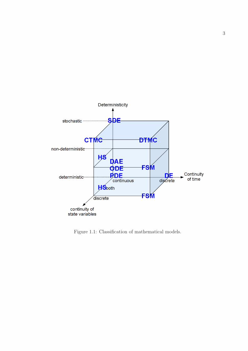
1.1 Classification of mathematical models. . . . . . . . . . . . . . . . . . . . . . 3

2.1 A model consisting of two separate sub-systems. . . . . . . . . . . . . . . . . 142.2 A model consisting of a nonlinear sub-system and a linear sub-system. . . . . 152.3 A model consisting of two identical sub-systems. . . . . . . . . . . . . . . . . 15

3.1 Relationship amongMr,LTI,Mr,V andMr,V . . . . . . . . . . . . . . . . . . 27

4.1 Trajectories of (4.1) in the state space. . . . . . . . . . . . . . . . . . . . . . 374.2 Trajectories of (4.2) in the state space. . . . . . . . . . . . . . . . . . . . . . 38

5.1 Simulation of the ManiMOR model. (u(t) = t) Fig. 5.1(a) shows the manifoldManiMOR identifies (yellow), and the trajectories of the full model (blue)and ManiMOR model (green). Fig. 5.1(b) shows the waveform of x3(t) of theManiMOR model (green), the full model (blue), and the projection of the fullmodel solution onto the manifold (black). . . . . . . . . . . . . . . . . . . . 63

5.2 Simulation of the ManiMOR model. (sinusoidal input) Fig. 5.2(a) shows theDC curve (red) and the manifold ManiMOR identifies (yellow), the trajecto-ries of the full model (blue) and ManiMOR model (green). Fig. 5.2(b) showsthe waveform of x3(t) of the ManiMOR model (green), the full model (blue),and the projection of the full model solution onto the manifold (black). . . . 64

5.3 Comparison of ManiMOR and TPWL model. (multiple-step input) Red,green and blue trajectories represent simulation results of ManiMOR, TPWLand full model, respectively. . . . . . . . . . . . . . . . . . . . . . . . . . . . 65

5.4 Comparison of ManiMOR and TPWL model. (two-tone sinusoidal input)Red, green and blue trajectories represent simulation results of ManiMOR,TPWL and full model, respectively. . . . . . . . . . . . . . . . . . . . . . . 66

5.5 Circuit diagram of a CMOS ring mixer [1]. . . . . . . . . . . . . . . . . . . . 66

viii

5.6 Simulation of ManiMOR model and full model for the CMOS ring mixer. (stepinput) Fig. 5.6(a) shows the manifold ManiMOR identifies (yellow), and thetrajectories of the full model (blue) and ManiMOR model (green). Fig. 5.6(b)shows the waveform of x3(t) of the ManiMOR model (green), the full model(blue), and the projection of the full model result onto the constructed man-ifold (black). . . . . . . . . . . . . . . . . . . . . . . . . . . . . . . . . . . . 67

5.7 Comparison of of the circuit response of ManiMOR model and TPWL model.(Nonlinear transmission line circuit [2]) . . . . . . . . . . . . . . . . . . . . 68

5.8 Circuit diagram of a current-model logic (CML) buffer. . . . . . . . . . . . . 685.9 Visualization of the low-order manifold subspace generated by ManiMOR. The

axes represent three node voltages in the circuit. The red curve consists ofthe DC operating points; the black dashed lines are the second local subspacebases; the yellow manifold is generated by stitching together all the local linearsubspaces. The blue circled points are on a transient trajectory simulatedusing the full model. . . . . . . . . . . . . . . . . . . . . . . . . . . . . . . . 69

5.10 Singular values of the matrix containing 20 equilibrium points, sorted. . . . . 705.11 Comparison of ManiMOR model with linearized reduced-order model. The

waveforms of one output using different models are plotted. . . . . . . . . . . 715.12 Comparison of ManiMOR model with TPWL model. The waveforms of one

output voltage using different models are plotted. . . . . . . . . . . . . . . . 725.13 Components of the pheromone response pathway in yeast. [3] Each arrow

represents a type of reaction. . . . . . . . . . . . . . . . . . . . . . . . . . . . 735.14 Concentrations of x1 at equilibrium corresponding to different inputs, and the

singular values for the DC matrix. . . . . . . . . . . . . . . . . . . . . . . . . 745.15 Transient simulation of the yeast pheromone pathway. The concentration of

one reactant is plotted. . . . . . . . . . . . . . . . . . . . . . . . . . . . . . . 75

6.1 QLMOR flow (yellow), with comparison to MOR based on polynomial form(green) and bilinear form (gray). . . . . . . . . . . . . . . . . . . . . . . . . . 81

6.2 A simple CMOS circuit. . . . . . . . . . . . . . . . . . . . . . . . . . . . . . 896.3 Polynomial approximations of 1/(1 + x). Fig. 6.3(a) shows the interval x ∈

[0, 1]. Fig. 6.3(b) shows the interval x ∈ [0, 2]. . . . . . . . . . . . . . . . . . . 1036.4 Fig. 6.4(a), Fig. 6.4(b) show the time-domain waveforms of x1, x2 and Fourier

coefficients of x1, respectively, when u(t) = cos(4πt). Fig. 6.4(c), Fig. 6.4(d)show the time-domain waveforms of x1, x2 and Fourier coefficients of x1, re-spectively, when u(t) = 10 cos(2πt). . . . . . . . . . . . . . . . . . . . . . . 104

6.5 Fig. 6.5(a), Fig. 6.5(b) show the time-domain waveforms of x1, x2 and Fouriercoefficients of x1, respectively, when u(t) = 8 cos(3πt). Fig. 6.5(c), Fig. 6.5(d)show the time-domain waveforms of x1, x2 and Fourier coefficients of x1, re-spectively, when u(t) = 10 cos(3πt). . . . . . . . . . . . . . . . . . . . . . . 106

6.6 Nonlinear transmission line circuit [2]. . . . . . . . . . . . . . . . . . . . . . 107

ix

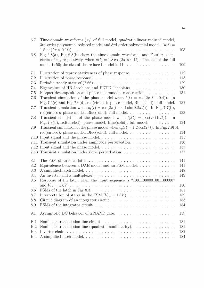
6.7 Time-domain waveforms (x1) of full model, quadratic-linear reduced model,3rd-order polynomial reduced model and 3rd-order polynomial model. (u(t) =1.8 sin(2π × 0.1t)) . . . . . . . . . . . . . . . . . . . . . . . . . . . . . . . . . 108

6.8 Fig. 6.8(a), Fig. 6.8(b) show the time-domain waveforms and Fourier coeffi-cients of x1, respectively, when u(t) = 1.8 cos(2π × 0.1t). The size of the fullmodel is 50; the size of the reduced model is 11. . . . . . . . . . . . . . . . . 109

7.1 Illustration of representativeness of phase response. . . . . . . . . . . . . . . 1127.2 Illustration of phase response. . . . . . . . . . . . . . . . . . . . . . . . . . . 1137.3 Periodic steady state of (7.66). . . . . . . . . . . . . . . . . . . . . . . . . . . 1297.4 Eigenvalues of HB Jacobians and FDTD Jacobians. . . . . . . . . . . . . . . 1307.5 Floquet decomposition and phase macromodel construction. . . . . . . . . . 1317.6 Transient simulation of the phase model when b(t) = cos(2π(t + 0.4)). In

Fig. 7.6(c) and Fig. 7.6(d), red(circled): phase model, Blue(solid): full model. 1327.7 Transient simulation when bp(t) = cos(2π(t + 0.1 sin(0.2πt))). In Fig. 7.7(b),

red(circled): phase model, Blue(solid): full model. . . . . . . . . . . . . . . . 1337.8 Transient simulation of the phase model when bp(t) = cos(2π(1.2t)). In

Fig. 7.8(b), red(circled): phase model, Blue(solid): full model. . . . . . . . . 1347.9 Transient simulation of the phase model when bp(t) = 1.2 cos(2πt). In Fig. 7.9(b),

red(circled): phase model, Blue(solid): full model. . . . . . . . . . . . . . . . 1347.10 Input signal and the phase model. . . . . . . . . . . . . . . . . . . . . . . . . 1357.11 Transient simulation under amplitude perturbation. . . . . . . . . . . . . . . 1367.12 Input signal and the phase model. . . . . . . . . . . . . . . . . . . . . . . . . 1377.13 Transient simulation under slope perturbation. . . . . . . . . . . . . . . . . . 137

8.1 The FSM of an ideal latch. . . . . . . . . . . . . . . . . . . . . . . . . . . . . 1418.2 Equivalence between a DAE model and an FSM model. . . . . . . . . . . . . 1418.3 A simplified latch model. . . . . . . . . . . . . . . . . . . . . . . . . . . . . . 1488.4 An inverter and a multiplexer. . . . . . . . . . . . . . . . . . . . . . . . . . . 1498.5 Response of the latch when the input sequence is “10011000001001100000”

and Vsw = 1.6V . . . . . . . . . . . . . . . . . . . . . . . . . . . . . . . . . . . 1508.6 FSMs of the latch in Fig. 8.3. . . . . . . . . . . . . . . . . . . . . . . . . . . 1518.7 Interpretation of states in the FSM (Vsw = 1.6V ). . . . . . . . . . . . . . . . 1528.8 Circuit diagram of an integrator circuit. . . . . . . . . . . . . . . . . . . . . 1538.9 FSMs of the integrator circuit. . . . . . . . . . . . . . . . . . . . . . . . . . . 154

9.1 Asymptotic DC behavior of a NAND gate. . . . . . . . . . . . . . . . . . . . 157

B.1 Nonlinear transmission line circuit. . . . . . . . . . . . . . . . . . . . . . . . 181B.2 Nonlinear transmission line (quadratic nonlinearity). . . . . . . . . . . . . . 181B.3 Inverter chain. . . . . . . . . . . . . . . . . . . . . . . . . . . . . . . . . . . . 182B.4 A simplified latch model. . . . . . . . . . . . . . . . . . . . . . . . . . . . . . 184

x

B.5 An inverter and a multiplexer. . . . . . . . . . . . . . . . . . . . . . . . . . . 185

xi

List of Tables

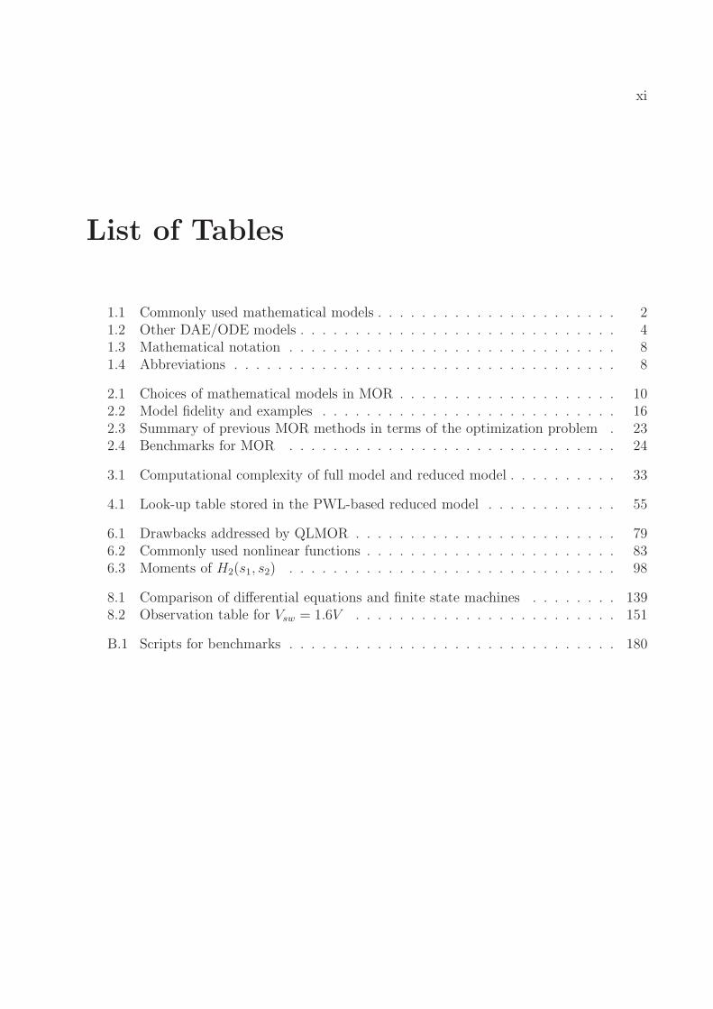
1.1 Commonly used mathematical models . . . . . . . . . . . . . . . . . . . . . . 21.2 Other DAE/ODE models . . . . . . . . . . . . . . . . . . . . . . . . . . . . . 41.3 Mathematical notation . . . . . . . . . . . . . . . . . . . . . . . . . . . . . . 81.4 Abbreviations . . . . . . . . . . . . . . . . . . . . . . . . . . . . . . . . . . . 8

2.1 Choices of mathematical models in MOR . . . . . . . . . . . . . . . . . . . . 102.2 Model fidelity and examples . . . . . . . . . . . . . . . . . . . . . . . . . . . 162.3 Summary of previous MOR methods in terms of the optimization problem . 232.4 Benchmarks for MOR . . . . . . . . . . . . . . . . . . . . . . . . . . . . . . 24

3.1 Computational complexity of full model and reduced model . . . . . . . . . . 33

4.1 Look-up table stored in the PWL-based reduced model . . . . . . . . . . . . 55

6.1 Drawbacks addressed by QLMOR . . . . . . . . . . . . . . . . . . . . . . . . 796.2 Commonly used nonlinear functions . . . . . . . . . . . . . . . . . . . . . . . 836.3 Moments of H2(s1, s2) . . . . . . . . . . . . . . . . . . . . . . . . . . . . . . 98

8.1 Comparison of differential equations and finite state machines . . . . . . . . 1398.2 Observation table for Vsw = 1.6V . . . . . . . . . . . . . . . . . . . . . . . . 151

B.1 Scripts for benchmarks . . . . . . . . . . . . . . . . . . . . . . . . . . . . . . 180

1

Chapter 1

Introduction

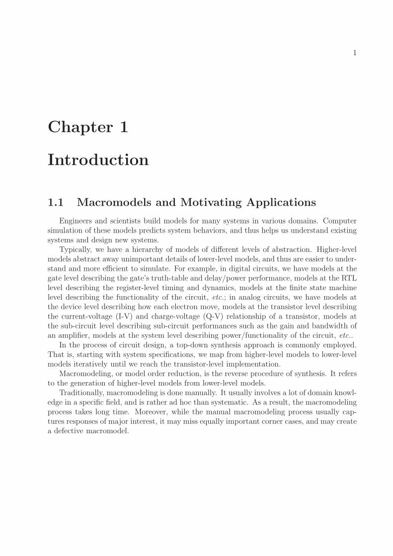
1.1 Macromodels and Motivating Applications

Engineers and scientists build models for many systems in various domains. Computersimulation of these models predicts system behaviors, and thus helps us understand existingsystems and design new systems.

Typically, we have a hierarchy of models of different levels of abstraction. Higher-levelmodels abstract away unimportant details of lower-level models, and thus are easier to under-stand and more efficient to simulate. For example, in digital circuits, we have models at thegate level describing the gate’s truth-table and delay/power performance, models at the RTLlevel describing the register-level timing and dynamics, models at the finite state machinelevel describing the functionality of the circuit, etc.; in analog circuits, we have models atthe device level describing how each electron move, models at the transistor level describingthe current-voltage (I-V) and charge-voltage (Q-V) relationship of a transistor, models atthe sub-circuit level describing sub-circuit performances such as the gain and bandwidth ofan amplifier, models at the system level describing power/functionality of the circuit, etc..

In the process of circuit design, a top-down synthesis approach is commonly employed.That is, starting with system specifications, we map from higher-level models to lower-levelmodels iteratively until we reach the transistor-level implementation.

Macromodeling, or model order reduction, is the reverse procedure of synthesis. It refersto the generation of higher-level models from lower-level models.

Traditionally, macromodeling is done manually. It usually involves a lot of domain knowl-edge in a specific field, and is rather ad hoc than systematic. As a result, the macromodelingprocess takes long time. Moreover, while the manual macromodeling process usually cap-tures responses of major interest, it may miss equally important corner cases, and may createa defective macromodel.

2

1.1.1 Mathematical Models

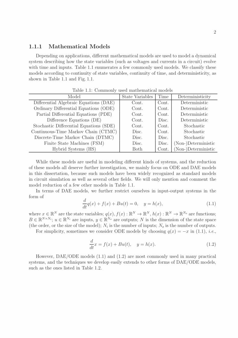
Depending on applications, different mathematical models are used to model a dynamicalsystem describing how the state variables (such as voltages and currents in a circuit) evolvewith time and inputs. Table 1.1 enumerates a few commonly used models. We classify thesemodels according to continuity of state variables, continuity of time, and deterministicity, asshown in Table 1.1 and Fig. 1.1.

Table 1.1: Commonly used mathematical models

Model State Variables Time DeterministicityDifferential Algebraic Equations (DAE) Cont. Cont. DeterministicOrdinary Differential Equations (ODE) Cont. Cont. DeterministicPartial Differential Equations (PDE) Cont. Cont. Deterministic

Difference Equations (DE) Cont. Disc. DeterministicStochastic Differential Equations (SDE) Cont. Cont. StochasticContinuous-Time Markov Chain (CTMC) Disc. Cont. StochasticDiscrete-Time Markov Chain (DTMC) Disc. Disc. Stochastic

Finite State Machines (FSM) Disc. Disc. (Non-)DeterministicHybrid Systems (HS) Both Cont. (Non-)Deterministic

While these models are useful in modeling different kinds of systems, and the reductionof these models all deserve further investigation, we mainly focus on ODE and DAE modelsin this dissertation, because such models have been widely recognized as standard modelsin circuit simulation as well as several other fields. We will only mention and comment themodel reduction of a few other models in Table 1.1.

In terms of DAE models, we further restrict ourselves in input-output systems in theform of

d

dtq(x) + f(x) +Bu(t) = 0, y = h(x), (1.1)

where x ∈ RN are the state variables; q(x), f(x) : RN → R

N , h(x) : RN → RNo are functions;

B ∈ RN×Ni; u ∈ R

Ni are inputs, y ∈ RNo are outputs; N is the dimension of the state space

(the order, or the size of the model); Ni is the number of inputs; No is the number of outputs.For simplicity, sometimes we consider ODE models by choosing q(x) = −x in (1.1), i.e.,

d

dtx = f(x) +Bu(t), y = h(x). (1.2)

However, DAE/ODE models (1.1) and (1.2) are most commonly used in many practicalsystems, and the techniques we develop easily extends to other forms of DAE/ODE models,such as the ones listed in Table 1.2.

3

Figure 1.1: Classification of mathematical models.

4

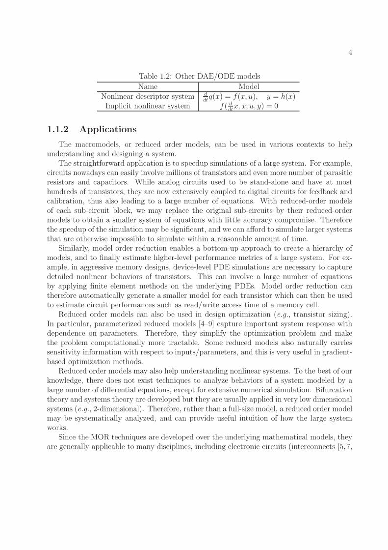
Table 1.2: Other DAE/ODE models

Name Model

Nonlinear descriptor system ddtq(x) = f(x, u), y = h(x)

Implicit nonlinear system f( ddtx, x, u, y) = 0

1.1.2 Applications

The macromodels, or reduced order models, can be used in various contexts to helpunderstanding and designing a system.

The straightforward application is to speedup simulations of a large system. For example,circuits nowadays can easily involve millions of transistors and even more number of parasiticresistors and capacitors. While analog circuits used to be stand-alone and have at mosthundreds of transistors, they are now extensively coupled to digital circuits for feedback andcalibration, thus also leading to a large number of equations. With reduced-order modelsof each sub-circuit block, we may replace the original sub-circuits by their reduced-ordermodels to obtain a smaller system of equations with little accuracy compromise. Thereforethe speedup of the simulation may be significant, and we can afford to simulate larger systemsthat are otherwise impossible to simulate within a reasonable amount of time.

Similarly, model order reduction enables a bottom-up approach to create a hierarchy ofmodels, and to finally estimate higher-level performance metrics of a large system. For ex-ample, in aggressive memory designs, device-level PDE simulations are necessary to capturedetailed nonlinear behaviors of transistors. This can involve a large number of equationsby applying finite element methods on the underlying PDEs. Model order reduction cantherefore automatically generate a smaller model for each transistor which can then be usedto estimate circuit performances such as read/write access time of a memory cell.

Reduced order models can also be used in design optimization (e.g., transistor sizing).In particular, parameterized reduced models [4–9] capture important system response withdependence on parameters. Therefore, they simplify the optimization problem and makethe problem computationally more tractable. Some reduced models also naturally carriessensitivity information with respect to inputs/parameters, and this is very useful in gradient-based optimization methods.

Reduced order models may also help understanding nonlinear systems. To the best of ourknowledge, there does not exist techniques to analyze behaviors of a system modeled by alarge number of differential equations, except for extensive numerical simulation. Bifurcationtheory and systems theory are developed but they are usually applied in very low dimensionalsystems (e.g., 2-dimensional). Therefore, rather than a full-size model, a reduced order modelmay be systematically analyzed, and can provide useful intuition of how the large systemworks.

Since the MOR techniques are developed over the underlying mathematical models, theyare generally applicable to many disciplines, including electronic circuits (interconnects [5,7,

5

10–14], electromagnetics [15–19], power grids [20–22], RF circuits [23–28], oscillators [29–32]),micro-electro-mechanical systems [33–39] fluid dynamics [40–46], biological systems [41, 47–51], neuroscience [52–59], chemical engineering [60–67], mechanical engineering [68–71], etc..

1.2 Problem Overview

Loosely speaking, model order reduction aims to generating “simpler” models that cap-ture “important” dynamics of original full models.

Here, “model” refers to a mathematical model that describes system behaviors. Themodel can be linear or nonlinear, continuous or discrete value, continuous or discrete time,deterministic or stochastic, as shown in Table 1.1.

“Simple” typically means computationally efficient, but may also represent other proper-ties of the model, such as sparsity of matrices in the model, number of parameters, numberof state variables, correlation among state variables, etc..

What “important” dynamics mean depends highly on applications. For examples, itcan be transfer functions over a certain frequency range (for LTI systems), the time-domainwaveforms, stability, passivity, etc..

For DAEs (1.1), model order reduction typically means deriving a system of reducedDAEs

d

dtqr(xr) + fr(xr) +Bru(t) = 0, y = hr(xr), (1.3)

where xr ∈ RNr are the state variables of the reduced model; qr(xr), fr(xr) : RNr → R

Nr ,hr(xr) : R

Nr → RNo are functions; B ∈ R

Nr×Ni; Nr is the order of the reduced model.

1.2.1 Challenges

While we will have more detailed discussions about challenges in nonlinear MOR inChapter 2 and other chapters, we highlight the major ones in this section.

1. Difficulties intrinsic in the current projection framework. LTI MOR techniques gen-erally are formulated within a linear projection framework. However, it may not beefficient/reasonable to use linear projection for nonlinear models, as it leads to lesscomputational speedup and lacks enough theoretical support, compared to LTI cases.It is worthwhile to investigate how nonlinear projections may work better than lin-ear projections, and that casts even more questions than answers regarding nonlinearmodel order reduction.

2. Lack of canonical representation of a nonlinear model. LTI models (linear differentialequations) C d

dtx + Gx + Bu = 0 have a very special and compact matrix represen-

tation (C,G,B). There are also other equivalent canonical representations such ascontrollable/observable canonical forms [72,73]. However, there have been hardly any

6

literature on canonical forms of general nonlinear systems. The nonlinear functionscan be arbitrary and complicated, making the system hard to analyze and manipulate,and even harder to reduce.

3. Lack of characterization of system responses. LTI systems can be characterized bytheir transfer functions which are extensively used as a performance metric to preservein linear model order reduction. However, for nonlinear systems, there is no simpleway to derive analytical expressions of system responses such as harmonic distortion,output frequency, etc.. This further complicates the reduction problem.

1.3 Dissertation Contributions and Overview

In this dissertation, we formulate the model order reduction problem, explore and de-velop nonlinear model order reduction techniques, and apply these techniques in practicalexamples. In particular, the main contributions are as follows:

1. We formulate the nonlinear model order reduction problem as an optimization problemand present a general nonlinear projection framework that encompasses previous linearprojection-based techniques as well as the techniques developed in this dissertation.

2. We develop a nonlinear model order reduction technique, ManiMOR, which is a di-rect implementation of the nonlinear projection framework. It generates a nonlinearreduced model by projection on a general-purpose nonlinear manifold. The proposedmanifold can be proven to capture important system dynamics such as DC and ACresponses. We develop numerical methods that alleviates the computational cost ofthe reduced model which is otherwise too expensive to make the reduced order modelof any value compared to the full model.

3. We develop a nonlinear model order reduction technique, QLMOR, which transformsthe full model to a canonical QLDAE representation and performs Volterra analysis toderive a reduced model. We develop an algorithm that can mechanically transform aset of nonlinear differential equations to another set of equivalent nonlinear differentialequations that involve only quadratic terms of state variables, and therefore it avoidsany problem brought by previous Taylor-expansion-based methods. With the QLDAErepresentation, we develop the corresponding model order reduction algorithm thatextends and generalizes previously-developed Volterra-based technique.

4. We develop a nonlinear phase/timing macromodeling technique, NTIM, that derivesa macromodel that specifically capture timing/phase responses of a nonlinear system.We rigorously define the phase response for a non-autonomous system, and derive thedynamics of the phase response. The macromodel emerges as a scalar, nonlinear time-varying differential equation that can be computed by performing Floquet analysis of

7

the full model. With the theory developed, we also present efficient numerical methodsto compute the macromodel.

5. We develop a finite state machine abstraction technique, DAE2FSM, that learns aMealy machine from a set of differential equations from its input-output trajectories.The algorithm explores the state space in a smart way so that it can identify the under-lying finite state machine using very few information about input-output trajectories.

The remainder of the dissertation is organized as follows. Chapter 2 formulates the MORproblem, reviews previous work and summarizes challenges in nonlinear MOR. Chapter 3provides a deeper view of the linear projection framework that is used by most previousMOR methods. Chapter 4 generalizes the linear projection framework to a nonlinear one,and summarizes the skeleton of an algorithm within this framework. Chapter 5 presentsthe method ManiMOR that is a direct implementation of the nonlinear projection frame-work. Chapter 6 presents the method QLMOR that generates a quadratic-linear reducedorder model. Chapter 7 presents the method NTIM that generates a phase/timing reducedmodel. Both QLMOR and NTIM can be interpreted in the nonlinear projection framework.Chapter 8 looks at a slightly different problem of deriving a finite state machine model froma set of differential equations, and presents the method DAE2FSM. Chapter 9 concludes thedissertation and discusses the related future work.

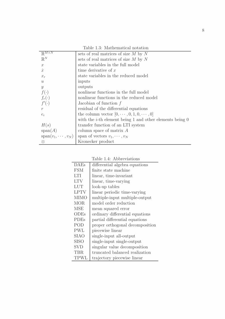
1.4 Notations and Abbreviations

Except for special mention, we will use use the following notations and abbreviationsthroughout the dissertation.

8

Table 1.3: Mathematical notation

RM×N sets of real matrices of size M by N

RN sets of real matrices of size M by N

x state variables in the full modelx time derivative of xxr state variables in the reduced modelu inputsy outputsf(·) nonlinear functions in the full modelfr(·) nonlinear functions in the reduced modelf ′(·) Jacobian of function fr residual of the differential equationsei the column vector [0, · · · , 0, 1, 0, · · · , 0]

with the i-th element being 1 and other elements being 0H(s) transfer function of an LTI systemspan(A) column space of matrix Aspan(v1, · · · , vN) span of vectors v1, · · · , vN⊗ Kronecker product

Table 1.4: Abbreviations

DAEs differential algebra equationsFSM finite state machineLTI linear, time-invariantLTV linear, time-varyingLUT look-up tablesLPTV linear periodic time-varyingMIMO multiple-input multiple-outputMOR model order reductionMSE mean squared errorODEs ordinary differential equationsPDEs partial differential equationsPOD proper orthogonal decompositionPWL piecewise linearSIAO single-input all-outputSISO single-input single-outputSVD singular value decompositionTBR truncated balanced realizationTPWL trajectory piecewise linear

9

Chapter 2

Background and Previous Work

In this chapter, we formally formulate the model order reduction problem, trying toencompass all previous methods under the same formulation. We review previous linear andnonlinear model order reduction techniques, and summarize a few challenges in nonlinearMOR, some of which are addressed in this dissertation.

2.1 Problem Formulation

Suppose that we are given a full model M ∈M, whereM is the set of a specific type ofmodel, (e.g., ordinary differential equations). The goal of model order reduction is to derivea reduced model Mr ∈ Mr, where Mr is the set of another type of models (e.g., ordinarydifferential equations), so that Mr approximates M in some sense.

Mathematically, we can define the problem of computing Mr from M as the followingoptimization problem

minimizeMr

F (M,Mr)

subject to G(M,Mr) = 0,

H(M,Mr) ≤ 0,

(2.1)

where F (·, ·), G(·, ·), H(·, ·) are functions on models M and Mr. F (·, ·) specifies how closetwo models are. G(·, ·) and H(·, ·) specify the equality and inequality constraints.

Choices ofM, Mr, F (·, ·), G(·, ·) and H(·, ·) lead to different problems. Usually, if Mr

has less number of state variables (i.e., the order of the system) thanM , it is called a reducedorder model, and Mr is expected to be computationally more efficient than M .

2.1.1 Types of Models

As listed in Table 1.1, there are many types of mathematical models. However, in theMOR problem, not all pairs of models (M,Mr) are reasonable. For example, it may be

10

unreasonable to reduce an LTI model to a nonlinear model because they may exhibit funda-mentally different behaviors; it may also be unreasonable to convert a deterministic modelto a non-deterministic one and vise versa.

In this dissertation, unless otherwise mentioned, we focus on the problem whereM andMr are both linear ODEs/DAEs or nonlinear ODEs/DAEs.

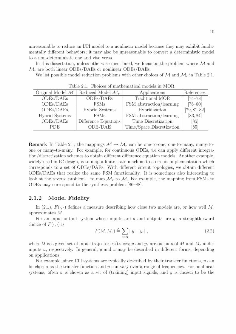
We list possible model reduction problems with other choices ofM andMr in Table 2.1.

Table 2.1: Choices of mathematical models in MOR

Original ModelM Reduced ModelMr Applications ReferencesODEs/DAEs ODEs/DAEs Traditional MOR [74–78]ODEs/DAEs FSMs FSM abstraction/learning [78–80]ODEs/DAEs Hybrid Systems Hybridization [79, 81, 82]

Hybrid Systems FSMs FSM abstraction/learning [83, 84]ODEs/DAEs Difference Equations Time Discretization [85]

PDE ODE/DAE Time/Space Discretization [85]

Remark In Table 2.1, the mappingsM→Mr can be one-to-one, one-to-many, many-to-one or many-to-many. For example, for continuous ODEs, we can apply different integra-tion/discretization schemes to obtain different difference equation models. Another example,widely used in IC design, is to map a finite state machine to a circuit implementation whichcorresponds to a set of ODEs/DAEs. With different circuit topologies, we obtain differentODEs/DAEs that realize the same FSM functionality. It is sometimes also interesting tolook at the reverse problem – to mapMr toM. For example, the mapping from FSMs toODEs may correspond to the synthesis problem [86–88].

2.1.2 Model Fidelity

In (2.1), F (·, ·) defines a measure describing how close two models are, or how well Mr

approximates M .For an input-output system whose inputs are u and outputs are y, a straightforward

choice of F (·, ·) isF (M,Mr) ,

∑

u∈U

||y − yr||, (2.2)

where U is a given set of input trajectories/traces; y and yr are outputs of M and Mr underinputs u, respectively. In general, y and u may be described in different forms, dependingon applications.

For example, since LTI systems are typically described by their transfer functions, y canbe chosen as the transfer function and u can vary over a range of frequencies. For nonlinearsystems, often u is chosen as a set of (training) input signals, and y is chosen to be the

11

corresponding time-domain responses, or the first few harmonic distortions when the systemis settled at the periodic steady state. In specific applications where other special responsesor higher-level performance metrics (such as phase/timing responses or bit error rate) are ofinterest, y can also be set to these quantities.

There have also been many techniques in reducing dynamical systems with no inputs(e.g., the ODE model x = f(x)). In this case, we may still view it as an input-outputsystem, with the virtual input to the system being the set of all possible impulse functionsthat set the initial condition of the system when applied. These methods basically computereduced order models that approximate outputs of full models for arbitrary initial conditions.

G(·, ·) and H(·, ·) in (2.1) impose equality and inequality constraints on the reducedorder model, respectively. They are usually used to guarantee certain important behaviorsof reduced models.

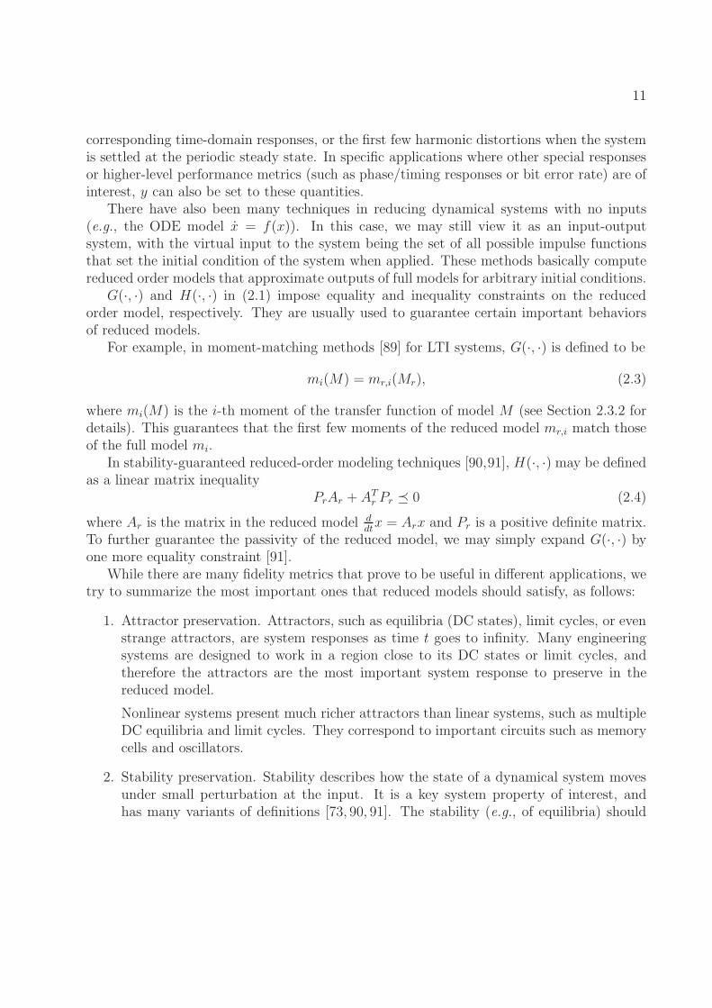
For example, in moment-matching methods [89] for LTI systems, G(·, ·) is defined to be

mi(M) = mr,i(Mr), (2.3)

where mi(M) is the i-th moment of the transfer function of model M (see Section 2.3.2 fordetails). This guarantees that the first few moments of the reduced model mr,i match thoseof the full model mi.

In stability-guaranteed reduced-order modeling techniques [90,91], H(·, ·) may be definedas a linear matrix inequality

PrAr + ATr Pr 0 (2.4)

where Ar is the matrix in the reduced model ddtx = Arx and Pr is a positive definite matrix.

To further guarantee the passivity of the reduced model, we may simply expand G(·, ·) byone more equality constraint [91].

While there are many fidelity metrics that prove to be useful in different applications, wetry to summarize the most important ones that reduced models should satisfy, as follows:

1. Attractor preservation. Attractors, such as equilibria (DC states), limit cycles, or evenstrange attractors, are system responses as time t goes to infinity. Many engineeringsystems are designed to work in a region close to its DC states or limit cycles, andtherefore the attractors are the most important system response to preserve in thereduced model.

Nonlinear systems present much richer attractors than linear systems, such as multipleDC equilibria and limit cycles. They correspond to important circuits such as memorycells and oscillators.

2. Stability preservation. Stability describes how the state of a dynamical system movesunder small perturbation at the input. It is a key system property of interest, andhas many variants of definitions [73, 90, 91]. The stability (e.g., of equilibria) should

12

be preserved in the reduced model since it ensures that the qualitative behavior of thesystem is correct, given that the attractors are preserved in the model.

3. Passivity preservation. Passivity of a system refers to the property that the systemonly consumes energy and never produces energy. This is commonly seen in practicalsystems, such as RLC interconnects. This is another qualitative behavior of a system,and is desirably preserved in reduced models.

4. Structure preservation. Reduced models are often written as a set of dense (in termsof Jacobian matrices) and less structured differential equations. However, full modelsusually have certain structures. For example, the system matrices may be sparse,symmetric or have block patterns; the system may be composed of a cascade of severalsub-systems, or a feedback; the system may be be a second order system; the systemmay obey certain conservation laws; the system may correspond to a realistic circuitimplementation. Therefore, it is sometimes desirable for reduced models to preservethese structures, even with certain accuracy loss.

5. Linearity preservation. This refers to the property that the reduced model of a linearsystem should remain linear. This is rather a necessary condition that should beappreciated in practice, especially for nonlinear MOR techniques. Linear systems havelimited behaviors than nonlinear systems, and should not exhibit any nonlinear effectsinduced by model reduction methods.

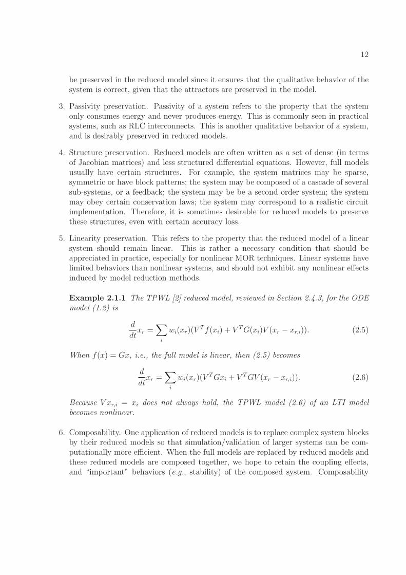
Example 2.1.1 The TPWL [2] reduced model, reviewed in Section 2.4.3, for the ODEmodel (1.2) is

d

dtxr =

∑

i

wi(xr)(VTf(xi) + V TG(xi)V (xr − xr,i)). (2.5)

When f(x) = Gx, i.e., the full model is linear, then (2.5) becomes

d

dtxr =

∑

i

wi(xr)(VTGxi + V TGV (xr − xr,i)). (2.6)

Because V xr,i = xi does not always hold, the TPWL model (2.6) of an LTI modelbecomes nonlinear.

6. Composability. One application of reduced models is to replace complex system blocksby their reduced models so that simulation/validation of larger systems can be com-putationally more efficient. When the full models are replaced by reduced models andthese reduced models are composed together, we hope to retain the coupling effects,and “important” behaviors (e.g., stability) of the composed system. Composability

13

also allows one to generate reduced models of sub-systems separately and obtain re-duced models of larger sub-systems by composition. It can lead to a hierarchical modelorder reduction framework.

7. Identification of simpler models under coordinate transformation. A nonlinear system,in some cases, can be converted to a simpler model (e.g., with less nonlinearity), oreven to an LTI model. In such cases, the nonlinear MOR problem may be reduced toa linear MOR problem, and therefore becomes much easier. One such example is asfollows:

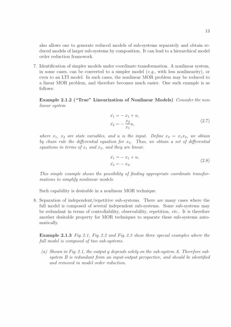
Example 2.1.2 (“True” Linearization of Nonlinear Models) Consider the non-linear system

x1 =− x1 + u,

x2 =−x2

x1u,

(2.7)

where x1, x2 are state variables, and u is the input. Define x3 = x1x2, we obtainby chain rule the differential equation for x3. Thus, we obtain a set of differentialequations in terms of x1 and x3, and they are linear.

x1 =− x1 + u,

x3 =− x3.(2.8)

This simple example shows the possibility of finding appropriate coordinate transfor-mations to simplify nonlinear models.

Such capability is desirable in a nonlinear MOR technique.

8. Separation of independent/repetitive sub-systems. There are many cases where thefull model is composed of several independent sub-systems. Some sub-systems maybe redundant in terms of controllability, observability, repetition, etc.. It is thereforeanother desirable property for MOR techniques to separate these sub-systems auto-matically.

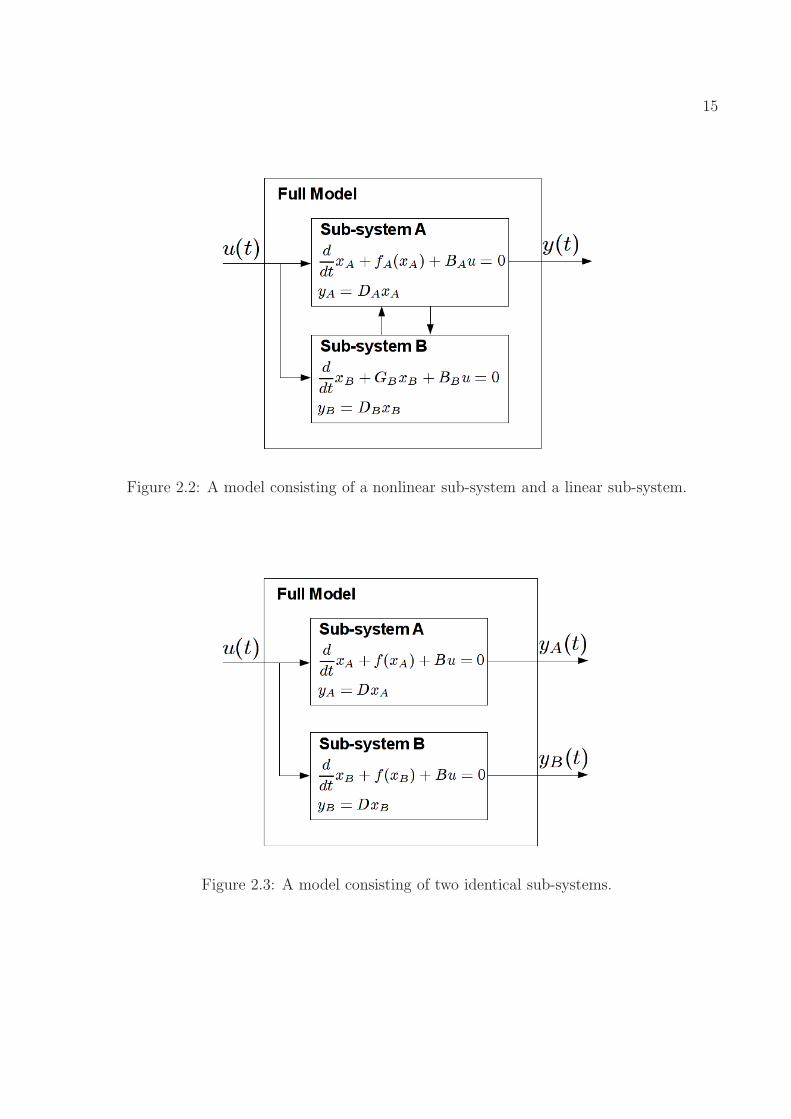
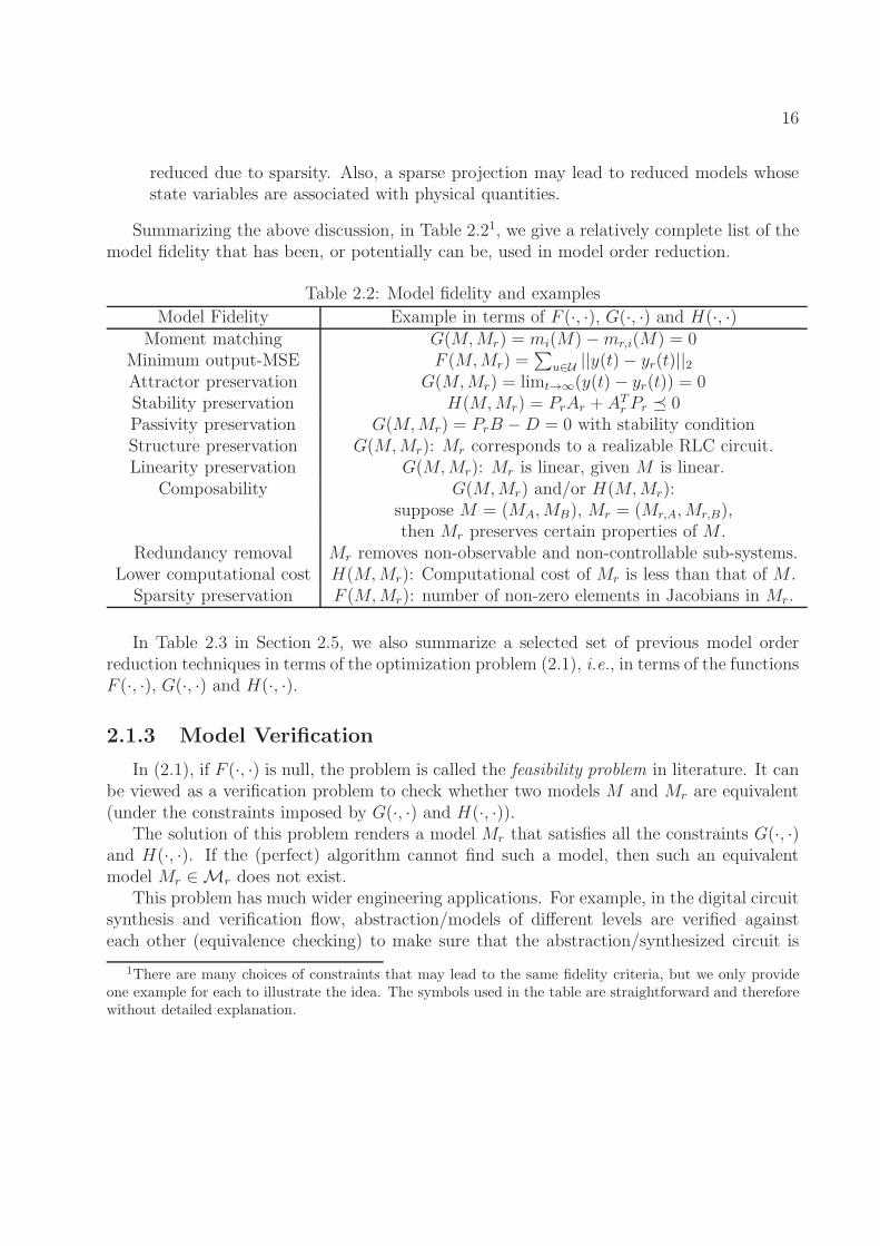
Example 2.1.3 Fig. 2.1, Fig. 2.2 and Fig. 2.3 show three special examples where thefull model is composed of two sub-systems.

(a) Shown in Fig. 2.1, the output y depends solely on the sub-system A. Therefore sub-system B is redundant from an input-output perspective, and should be identifiedand removed in model order reduction.

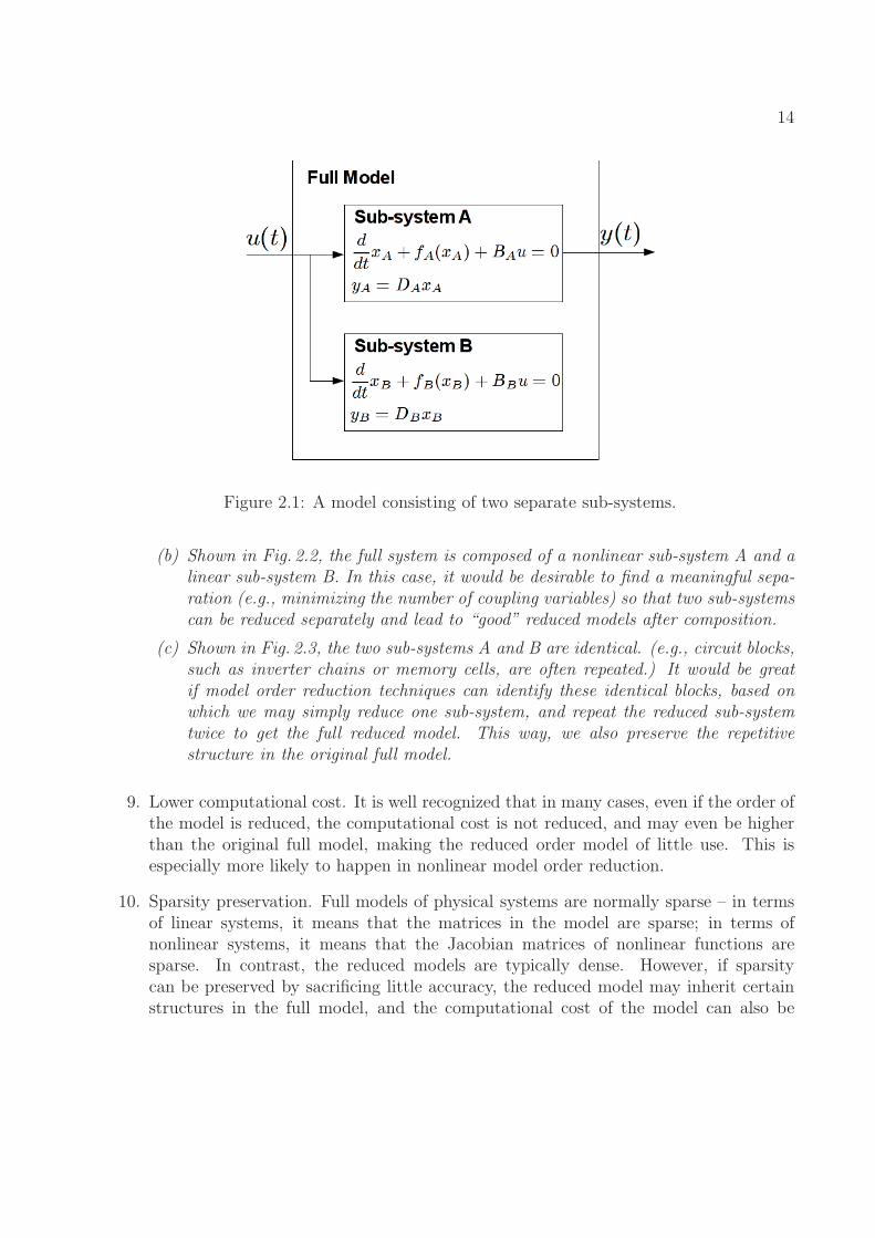
14

Figure 2.1: A model consisting of two separate sub-systems.

(b) Shown in Fig. 2.2, the full system is composed of a nonlinear sub-system A and alinear sub-system B. In this case, it would be desirable to find a meaningful sepa-ration (e.g., minimizing the number of coupling variables) so that two sub-systemscan be reduced separately and lead to “good” reduced models after composition.

(c) Shown in Fig. 2.3, the two sub-systems A and B are identical. (e.g., circuit blocks,such as inverter chains or memory cells, are often repeated.) It would be greatif model order reduction techniques can identify these identical blocks, based onwhich we may simply reduce one sub-system, and repeat the reduced sub-systemtwice to get the full reduced model. This way, we also preserve the repetitivestructure in the original full model.

9. Lower computational cost. It is well recognized that in many cases, even if the order ofthe model is reduced, the computational cost is not reduced, and may even be higherthan the original full model, making the reduced order model of little use. This isespecially more likely to happen in nonlinear model order reduction.

10. Sparsity preservation. Full models of physical systems are normally sparse – in termsof linear systems, it means that the matrices in the model are sparse; in terms ofnonlinear systems, it means that the Jacobian matrices of nonlinear functions aresparse. In contrast, the reduced models are typically dense. However, if sparsitycan be preserved by sacrificing little accuracy, the reduced model may inherit certainstructures in the full model, and the computational cost of the model can also be

15

Figure 2.2: A model consisting of a nonlinear sub-system and a linear sub-system.

Figure 2.3: A model consisting of two identical sub-systems.

16

reduced due to sparsity. Also, a sparse projection may lead to reduced models whosestate variables are associated with physical quantities.

Summarizing the above discussion, in Table 2.21, we give a relatively complete list of themodel fidelity that has been, or potentially can be, used in model order reduction.

Table 2.2: Model fidelity and examples

Model Fidelity Example in terms of F (·, ·), G(·, ·) and H(·, ·)Moment matching G(M,Mr) = mi(M)−mr,i(M) = 0

Minimum output-MSE F (M,Mr) =∑

u∈U ||y(t)− yr(t)||2Attractor preservation G(M,Mr) = limt→∞(y(t)− yr(t)) = 0Stability preservation H(M,Mr) = PrAr + AT

r Pr 0Passivity preservation G(M,Mr) = PrB −D = 0 with stability conditionStructure preservation G(M,Mr): Mr corresponds to a realizable RLC circuit.Linearity preservation G(M,Mr): Mr is linear, given M is linear.

Composability G(M,Mr) and/or H(M,Mr):suppose M = (MA,MB), Mr = (Mr,A,Mr,B),then Mr preserves certain properties of M .

Redundancy removal Mr removes non-observable and non-controllable sub-systems.Lower computational cost H(M,Mr): Computational cost of Mr is less than that of M .

Sparsity preservation F (M,Mr): number of non-zero elements in Jacobians in Mr.

In Table 2.3 in Section 2.5, we also summarize a selected set of previous model orderreduction techniques in terms of the optimization problem (2.1), i.e., in terms of the functionsF (·, ·), G(·, ·) and H(·, ·).

2.1.3 Model Verification

In (2.1), if F (·, ·) is null, the problem is called the feasibility problem in literature. It canbe viewed as a verification problem to check whether two models M and Mr are equivalent(under the constraints imposed by G(·, ·) and H(·, ·)).

The solution of this problem renders a model Mr that satisfies all the constraints G(·, ·)and H(·, ·). If the (perfect) algorithm cannot find such a model, then such an equivalentmodel Mr ∈Mr does not exist.

This problem has much wider engineering applications. For example, in the digital circuitsynthesis and verification flow, abstraction/models of different levels are verified againsteach other (equivalence checking) to make sure that the abstraction/synthesized circuit is

1There are many choices of constraints that may lead to the same fidelity criteria, but we only provideone example for each to illustrate the idea. The symbols used in the table are straightforward and thereforewithout detailed explanation.

17

functionally correct. Solving such problems is therefore the key enabler of the digital circuitdesign flow.

However, in model order reduction literature, this equivalence checking procedure istypically skipped, or is done by heuristics. We believe that this is an important problem tosolve for employing MOR in practice, and some initial studies [79, 92–96] in analog/mixed-signal verification may be used.

2.2 MOR Overview

According to the description of the full system, model order reduction methods can beclassified into black-box methods and white-box methods.

In black-box methods, the internal structure or representation of the model is not acces-sible. Rather, we have restricted access to only a few controllable inputs (e.g., stimulations)and observable outputs (e.g., from measurements or simulations). This leads to various“fitting” algorithms, including regression, neural network, machine learning, etc.. Thesemethods are often also called system identification methods. Due to the nature of suchmethods, we normally cannot assert any deterministic relationship between the full modeland the reduced model beyond the training data.

In white-box methods, we have full access to the model. This gives us a complete viewof the full model, and thus opportunities to guarantee certain properties can be preservedfrom full models. Depending on the type of the full model, the behavior can be qualitativelydifferent, and therefore different methods have been proposed to handle different types ofmodels, including LTI, LTV and nonlinear models. The most common framework encom-passing most of these methods is the linear projection framework, to be introduced in thissection, and detailed in Chapter 3.

2.2.1 System Identification

System identification methods [97,98] view the system as a black/grey box. Usually onlylimited number of input-output data/trajectory is given, either by simulation or measure-ment. Sometimes, partial information of the system is known (such as the connectivity ofa graph). These methods can be classified into two categories: parametric methods andnon-parametric methods.

In parametric methods, we make assumptions of the model structure for the system, andparameterize the model by certain key parameters. With the parameterized model, the dataare used to fit the model by solving for parameters that minimizes the error between the fittedmodel and the data. For example, we may use methods such as least squares, maximumlikelihood, maximum a posteriori probability estimation, compressed sensing, etc..

In non-parametric methods, we construct the model directly from data. For example, tofind an LTI model of a system, we can measure directly the impulse response or step response

18

to reconstruct the LTI system. To compute the transfer function at specific frequency points,we can measure directly the response to a sinusoidal input. Often the experiments arecarefully designed for the identification purpose in non-parametric methods.

2.2.2 Linear Projection Framework

In the linear projection framework, we consider the problem of reducing a model M ∈Mthat is a set of differential algebraic equations

d

dtq(x) + f(x) + b(t) = 0, (2.9)

to a reduced model Mr ∈Mr that is another set of differential algebraic equations

d

dtqr(xr) + fr(xr) + br(t) = 0, (2.10)

by projection.That is, the nonlinear functions in (2.10) are defined by projection, i.e.,

qr(xr) = W T q(V xr),

fr(xr) = W Tf(V xr),

br(t) = W T b(t),

(2.11)

where V,W ∈ RN×Nr are two projection matrices.

Therefore, the problem of MOR amounts to finding two appropriate projection matrices.

2.3 MOR for Linear Time-Invariant Systems

For an LTI system, q(x) = Cx and f(x) = Gx are linear functions of x, and often theinput is written in the form of b(t) = Bu(t), i.e.

Cd

dtx+Gx+Bu = 0, y = DTx, (2.12)

where C ∈ RN×N , G ∈ R

N×N , B ∈ RN×Ni , D ∈ R

N×No , Ni is the number of inputs and No

is the number of outputs.LTI reduced models are therefore in the form of

Crd

dtxr +Grxr +Bru = 0, y = DT

r xr, (2.13)

where Cr ∈ RNr×Nr , Gr ∈ R

Nr×Nr , Br ∈ RNr×Ni , Dr ∈ R

Nr×No , Nr is the order of the

19

reduced model.

2.3.1 Transfer Function Fitting

Since LTI models can be equivalently defined by their transfer functions H(s), a straight-forward model order reduction method is to fit a reduced transfer function Hr(s) that givesa good approximation to H(s).

The famous approach is the Pade approximation [99], i.e., to find a rational reducedtransfer function of the form

Hr(s) =a0 + a1s+ a2s

2 + · · ·+ amsm

b0 + b1s+ b2s2 + · · ·+ bnsn(2.14)

which satisfies

Hr(0) = H(0),

dk

dskHr(0) =

dk

dskH(0), k = 1, 2, · · · , m+ n,

(2.15)

where dk

dskH(0) is also referred to as the k-th moment of the transfer function. Therefore, any

LTI MOR method that leads to a reduced model satisfying (2.15) is also called a moment-matching method.

Intuitively, Pade approximation is good for MOR because a rational function is a goodfit for LTI transfer functions – the original transfer function H(s) is typically a rationalfunction given that there is no repeating poles. In fact, we may analytically write out H(s)of (2.12) as

H(s) = DT (sC +G)−1B, (2.16)

which is a rational function in s if the matrix G−1C has no repeating eigenvalues.There have been a series of work developed based on this idea, among which two major

ones are AWE [100] and PVL [101]. AWE [100] explicitly computes the moments and findsa Pade approximation Hr(s) with m = n−1 that matches these moments. PVL [101] avoidsnumerical inaccuracy in the explicit moment computation in AWE, and uses the Lanczosprocess to compute the Pade approximation of the transfer function.

2.3.2 Krylov-Subspace Methods

The explicit moment calculation in the Pade approximation methods can have seriousnumerical inaccuracy, and this inaccuracy will be inherited to the reduced model. Even withPVL, since it uses a transfer function representation of the LTI system, it is not directlyclear what the state-space ODE/DAE model of the reduced model is.

20

The source of error in explicit moment computation comes from the fact that higher-order moments tend to decay/grow at an exponential rate. To see that, we may derive theexpression of the i-th moment to be

mi = DT (G−1C)iB. (2.17)

Therefore, as i becomes large,mi depends approximately only on the eigenvalue ofG−1C withthe largest absolute value, and therefore will decay/grow exponentially, leading to significantnumerical inaccuracy.

Krylov-subspace methods [89] avoids the explicit moment calculation. It turns out thatif we choose V and W such that

span(V ) = KNr(G−1C,B) = span(G−1CB, (G−1C)2B, · · · , (G−1C)NrB,

span(W ) = KNr((G−1C)T , D) = span((G−1C)TD, ((G−1C)T )2B, · · · , ((G−1C)T )NrD),

(2.18)

then the projected reduced models with Cr = W TCV , Gr = W TGV , Br = W TB, Dr = V TDhave the property that the first 2Nr moments of the reduced transfer function match thoseof the full transfer function.

Moreover, the projection matrices V and W can be efficiently and accurately computed(e.g., Arnoldi and Lanczos algorithms [102, 103]). These algorithms are computationallyefficient and numerically stable even for large scale problems (e.g., sparse matrices of dimen-sion on the order of millions), and therefore enables the moment-matching technique to beapplicable to large-scale problems.

2.3.3 Truncated Balanced Realization

The method of truncated balanced realization (TBR) originated from control theory,based on the idea of controllability and observability [104]. Loosely speaking, certain statesin a dynamical system are hard to control and some others are hard to observe. The balancedrealization obtains a dynamical system whose state variables have equal controllability andobservability. Then, the truncation of the states that are hard to control and observe leadsto a reduced order model.

It turns out that the TBR method also falls in the linear projection framework. Ulti-mately, it defines two matrices V and W , and the reduced model is a projected model.

2.3.4 Proper Orthogonal Decomposition

Proper orthogonal decomposition (POD) is also a method that derives reduced modelsby linear projection. It takes several data/trajectories of the state variables, and constructsa linear subspace that minimizes certain error between the projected reduced model and the

21

full model.On the one hand, POD is general because it can take any trajectory of state variables.

Therefore, prior information of input signals and system dynamics can help generating abetter reduced order model. In can also be shown that if the trajectory is chosen to be theimpulse response of an LTI system, then one version of the POD is equivalent to the TBRmethod.

On the other hand, POD is less systematic than other methods in the sense that thereis no universal guideline in choosing a “good” trajectory. Therefore, it is possible to have“bad” trajectories that lead to “bad” reduced order models.

2.4 MOR for Nonlinear Systems

Nonlinear MOR methods are mostly built upon the LTI MOR methods. For so-calledweakly-nonlinear systems, we may approximate the nonlinear model by a local model, such asLTI, LTV, Volterra models. The reduction is then performed on the approximated model toobtain an approximated reduced model. For general nonlinear systems, we may approximatethe nonlinear model around several different regions in the state space, and reduce eachlinearized model using LTI MOR methods.

2.4.1 Linear Time-Varying Approximation and MOR

There are many practical systems that may be well-approximated by linear time-varyingsystems, partly because these systems are engineered to work under time-varying operatingpoints. For example, in RF circuits such as mixers, the local frequency input is fixed,rendering an approximate periodic time-varying system. Similarly, in switched-capacitorcircuits, the clock input is fixed, and the circuit is approximately working periodically undertwo modes (clock high and clock low).

The MOR methods in [25, 28] extends the notion of transfer function for LTI system totime-varying transfer functions. Then it can be shown that using a Pade-like approxima-tion, or an appropriate projection, we can obtain reduced order models whose time-varyingtransfer functions approximate the original one.

2.4.2 Volterra-Based Methods

Generally, for a nonlinear system, we may derive a Volterra series approximation [105]which approximates its local behavior. Therefore, instead of matching the moments oftransfer functions, we may match the moments of Volterra kernels (higher-order transferfunctions), and this leads to the Volterra-based MORmethods such as NORM [106] and [107].Since the Volterra series only converges when input is small, Volterra-based models are“small-signal” or “local” models.

22

Similar to Krylov subspace methods, in this case, we may also choose projection matricesV and W that cover a series of Krylov subspaces so that the projected models match thespecified moments of Volterra kernels.

2.4.3 Trajectory-Based Methods

Unlike Volterra-based methods, trajectory-based MOR methods generate “global” re-duced models, instead of “local” ones.

Among several variants of trajectory-based methods, the representative one is the TPWLmethod [2] whose algorithm is shown in Algorithm 1. The TPWL method identifies two linearsubspaces V and W , and generates the reduced model by linear projection. The subspacesV and W are the aggregated subspaces of many reduced models of linearized models (e.g.,Krylov subspaces of linearized models), therefore making sure that the moments of transferfunctions of reduced linearized models match those of the full linearized models. In order toachieve the computational efficiency of the reduced model, i.e., the computation of the termW Tf(V z), it uses a weighted-summation of linear functions to approximate W Tf(V z).

Algorithm 1 TPWL (Trajectory Piece-Wise Linear) Model Order Reduction

Inputs: Differential equations of the full model ddtq(x) + f(x) +Bu = 0.

Outputs: Two linear subspaces defined by the column span of V and W . Dif-ferential equations of the reduced model d

dtqr(xr) + fr(xr) + Bru = 0. where

qr(xr) =∑Ns

i=1wi(xr)(WTq(xi) + W TC(xi)V (xr − xr,i)), fr(xr) =

∑Ns

i=1wi(xr)(WTf(xi) +

W TG(xi)V (xr−xr,i)), Br = W TB, wi(xr) are weighting functions described in Section 2.4.3,Ns is the number of sample points.

1: Simulate the full model using a set of “training” input signals, and obtain a set oftrajectories.

2: Sample Ns points xi, i = 1, · · · , Ns on these trajectories as expansion points of thereduced model.

3: for all i = 1, · · · , Ns do4: Linearize the full model around each sample point xi

5: Compute the reduced linearized models, and obtain projection matrices Vi and Wi foreach reduced model.

6: end for7: Compute the projection matrix for the nonlinear model V = [V1, x1, · · · , Vk, xk], W =

[W1, x1, · · · ,Wk, xk].8: Compute W Tf(xi), W

TG(xi)V , W T q(xi), WTC(xi)V and W TB, and store them in the

reduced model.

23

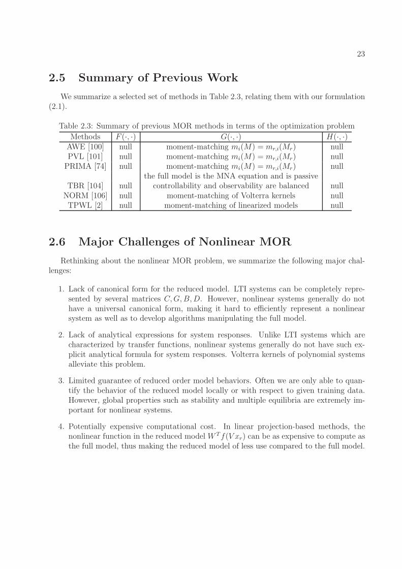
2.5 Summary of Previous Work

We summarize a selected set of methods in Table 2.3, relating them with our formulation(2.1).

Table 2.3: Summary of previous MOR methods in terms of the optimization problem

Methods F (·, ·) G(·, ·) H(·, ·)AWE [100] null moment-matching mi(M) = mr,i(Mr) nullPVL [101] null moment-matching mi(M) = mr,i(Mr) nullPRIMA [74] null moment-matching mi(M) = mr,i(Mr) null

the full model is the MNA equation and is passiveTBR [104] null controllability and observability are balanced null

NORM [106] null moment-matching of Volterra kernels nullTPWL [2] null moment-matching of linearized models null

2.6 Major Challenges of Nonlinear MOR

Rethinking about the nonlinear MOR problem, we summarize the following major chal-lenges:

1. Lack of canonical form for the reduced model. LTI systems can be completely repre-sented by several matrices C,G,B,D. However, nonlinear systems generally do nothave a universal canonical form, making it hard to efficiently represent a nonlinearsystem as well as to develop algorithms manipulating the full model.

2. Lack of analytical expressions for system responses. Unlike LTI systems which arecharacterized by transfer functions, nonlinear systems generally do not have such ex-plicit analytical formula for system responses. Volterra kernels of polynomial systemsalleviate this problem.

3. Limited guarantee of reduced order model behaviors. Often we are only able to quan-tify the behavior of the reduced model locally or with respect to given training data.However, global properties such as stability and multiple equilibria are extremely im-portant for nonlinear systems.

4. Potentially expensive computational cost. In linear projection-based methods, thenonlinear function in the reduced model W Tf(V xr) can be as expensive to compute asthe full model, thus making the reduced model of less use compared to the full model.

24

2.7 Benchmark Examples

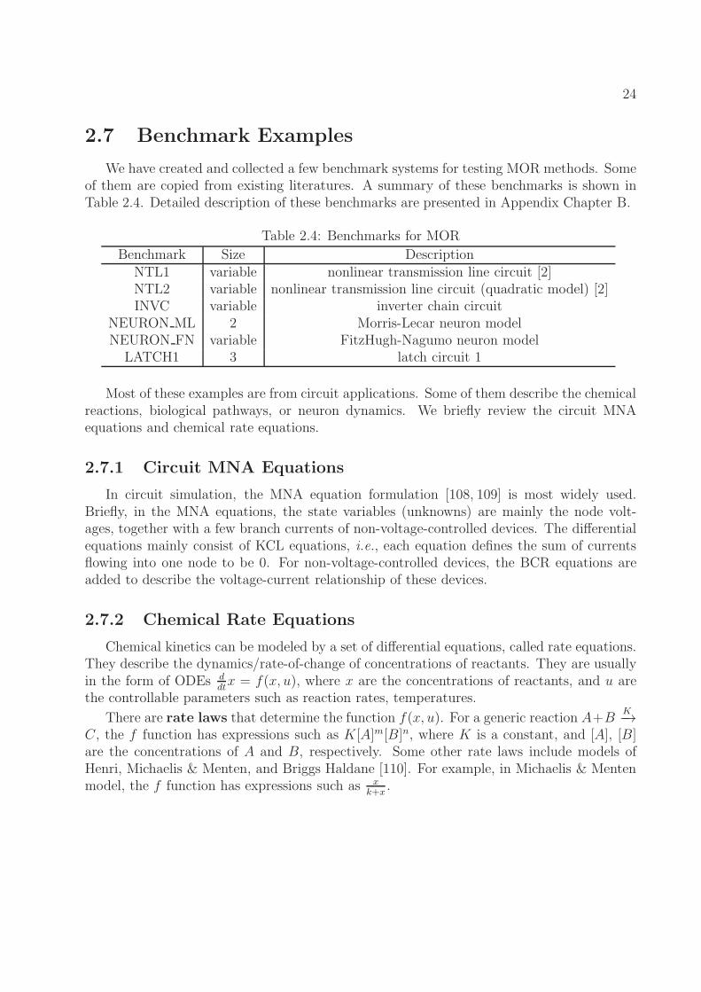
We have created and collected a few benchmark systems for testing MOR methods. Someof them are copied from existing literatures. A summary of these benchmarks is shown inTable 2.4. Detailed description of these benchmarks are presented in Appendix Chapter B.

Table 2.4: Benchmarks for MOR

Benchmark Size DescriptionNTL1 variable nonlinear transmission line circuit [2]NTL2 variable nonlinear transmission line circuit (quadratic model) [2]INVC variable inverter chain circuit

NEURON ML 2 Morris-Lecar neuron modelNEURON FN variable FitzHugh-Nagumo neuron model

LATCH1 3 latch circuit 1

Most of these examples are from circuit applications. Some of them describe the chemicalreactions, biological pathways, or neuron dynamics. We briefly review the circuit MNAequations and chemical rate equations.

2.7.1 Circuit MNA Equations

In circuit simulation, the MNA equation formulation [108, 109] is most widely used.Briefly, in the MNA equations, the state variables (unknowns) are mainly the node volt-ages, together with a few branch currents of non-voltage-controlled devices. The differentialequations mainly consist of KCL equations, i.e., each equation defines the sum of currentsflowing into one node to be 0. For non-voltage-controlled devices, the BCR equations areadded to describe the voltage-current relationship of these devices.

2.7.2 Chemical Rate Equations

Chemical kinetics can be modeled by a set of differential equations, called rate equations.They describe the dynamics/rate-of-change of concentrations of reactants. They are usuallyin the form of ODEs d

dtx = f(x, u), where x are the concentrations of reactants, and u are

the controllable parameters such as reaction rates, temperatures.

There are rate laws that determine the function f(x, u). For a generic reaction A+BK−→

C, the f function has expressions such as K[A]m[B]n, where K is a constant, and [A], [B]are the concentrations of A and B, respectively. Some other rate laws include models ofHenri, Michaelis & Menten, and Briggs Haldane [110]. For example, in Michaelis & Mentenmodel, the f function has expressions such as x

k+x.

25

Chapter 3

Linear Projection Framework forModel Order Reduction

While many previous MORmethods have used the linear projection framework, the majormotivation seems to be the fact that the projection of the full model on certain subspacesleads to a reduced model that matches certain accuracy metrics (e.g., moments or Hankelsingular values). However, no literature has discussed why such such a framework is a goodone for MOR. For example, some key questions that need to be answered are: can anyreduced model be written as a projected model; what is the degree of freedom in choosingprojection matrices; what might be other choices of projections; etc..

In this chapter, we take a deeper look at the linear projection framework. We discussthe application of the linear projection framework in LTI MOR – the representation powerof the linear projection framework, the degree of freedom in choosing projection matrices,the other potential criteria in choosing projection matrices. We also discuss the applicationof the linear projection framework in nonlinear MOR, and discuss potential problems andsolutions.

3.1 Linear Projection Framework

The basic idea of the linear projection work has already been presented in Section 2.2.2.Here, we focus on the algorithmic aspect of the linear projection framework. The problemis to reduce a model M ,

d

dtq(x) + f(x) + b(t) = 0, (3.1)

to a reduced model Mr,d

dtqr(xr) + fr(xr) + br(t) = 0. (3.2)

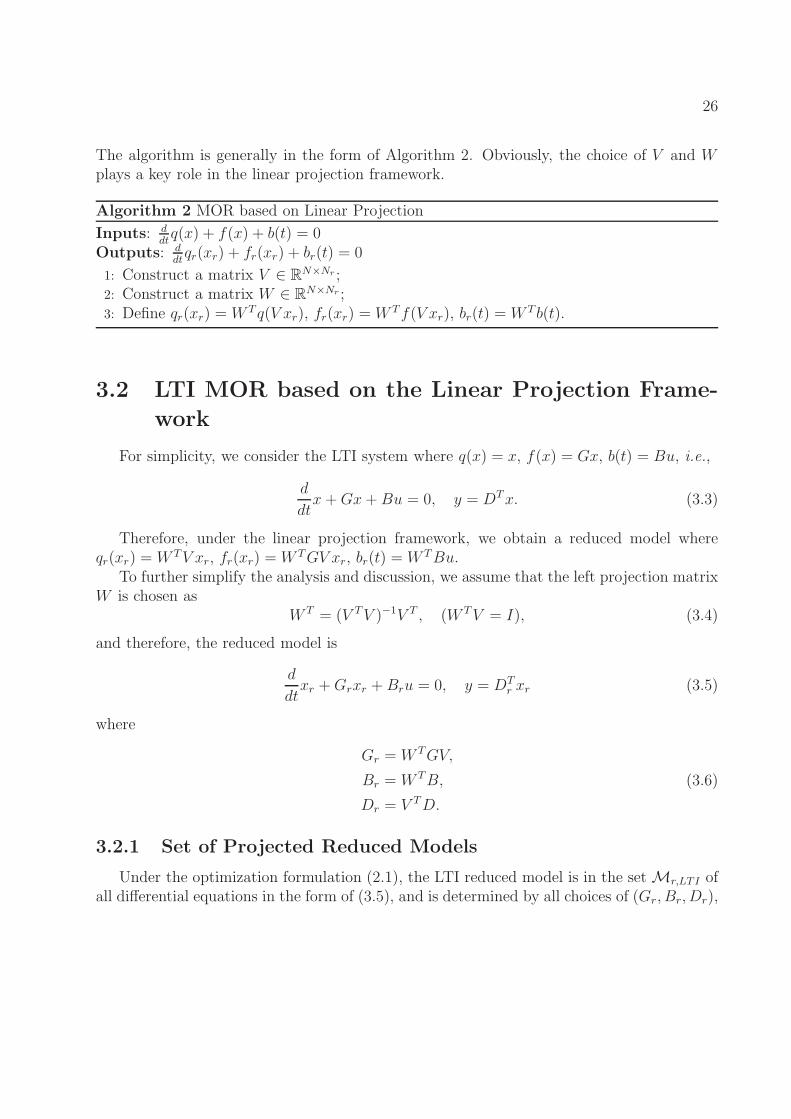
26

The algorithm is generally in the form of Algorithm 2. Obviously, the choice of V and Wplays a key role in the linear projection framework.

Algorithm 2 MOR based on Linear Projection

Inputs: ddtq(x) + f(x) + b(t) = 0

Outputs: ddtqr(xr) + fr(xr) + br(t) = 0

1: Construct a matrix V ∈ RN×Nr ;

2: Construct a matrix W ∈ RN×Nr ;

3: Define qr(xr) = W Tq(V xr), fr(xr) = W Tf(V xr), br(t) = W T b(t).

3.2 LTI MOR based on the Linear Projection Frame-

work

For simplicity, we consider the LTI system where q(x) = x, f(x) = Gx, b(t) = Bu, i.e.,

d

dtx+Gx+Bu = 0, y = DTx. (3.3)

Therefore, under the linear projection framework, we obtain a reduced model whereqr(xr) = W TV xr, fr(xr) = W TGV xr, br(t) = W TBu.

To further simplify the analysis and discussion, we assume that the left projection matrixW is chosen as

W T = (V TV )−1V T , (W TV = I), (3.4)

and therefore, the reduced model is

d


r xr (3.5)

where

Gr = W TGV,

Br = W TB,

Dr = V TD.

(3.6)

3.2.1 Set of Projected Reduced Models

Under the optimization formulation (2.1), the LTI reduced model is in the setMr,LTI ofall differential equations in the form of (3.5), and is determined by all choices of (Gr, Br, Dr),

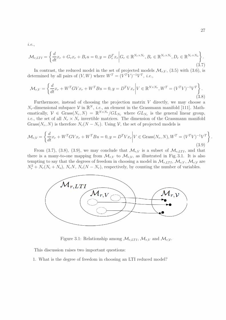
27

i.e.,

Mr,LTI =

d


r xr

∣

∣

∣

∣

Gr ∈ RNr×Nr , Br ∈ R

Nr×Ni, Dr ∈ RNr×No

.

(3.7)In contrast, the reduced model in the set of projected modelsMr,V , (3.5) with (3.6), is

determined by all pairs of (V,W ) where W T = (V TV )−1V T , i.e.,

Mr,V =

d

dtxr +W TGV xr +W TBu = 0, y = DTV xr

∣

∣

∣

∣

V ∈ RN×Nr ,W T = (V TV )−1V T

.

(3.8)Furthermore, instead of choosing the projection matrix V directly, we may choose a

Nr-dimensional subspace V in RN , i.e., an element in the Grassmann manifold [111]. Math-

ematically, V ∈ Grass(Nr, N) = RN×Nr/GLNr

where GLNris the general linear group,

i.e., the set of all Nr × Nr invertible matrices. The dimension of the Grassmann manifoldGrass(Nr, N) is therefore Nr(N −Nr). Using V, the set of projected models is

Mr,V =

d

dtxr +W TGV xr +W TBu = 0, y = DTV xr

∣

∣

∣

∣

V ∈ Grass(Nr, N),W T = (V TV )−1V T

.

(3.9)From (3.7), (3.8), (3.9), we may conclude that Mr,V is a subset of Mr,LTI , and that

there is a many-to-one mapping from Mr,V to Mr,V , as illustrated in Fig. 3.1. It is alsotempting to say that the degrees of freedom in choosing a model inMr,LTI ,Mr,V ,Mr,V areN2

r +Nr(Ni +No), NrN , Nr(N −Nr), respectively, by counting the number of variables.

Figure 3.1: Relationship amongMr,LTI ,Mr,V andMr,V .

This discussion raises two important questions:

1. What is the degree of freedom in choosing an LTI reduced model?

28

2. Are the projected models good candidates to use in MOR (i.e., do they encompass allpossible LTI reduced models)? If not, why are the projected models useful?

3.2.2 Degree of Freedom in Choosing SISO LTI Models

To determine the degree of freedom in choosing an LTI model in the form of (3.3),we study its canonical forms. Mathematically, given a set and an equivalent relation, thecanonical form is a unique representation of an equivalence class, i.e., all equivalent elementscan be mapped to the same canonical form. Therefore, by studying the canonical forms, wemay determine its degree of freedom.

For simplicity, we consider SISO systems in the following, i.e., Ni = No = 1. For SISOLTI systems, the canonical forms include transfer function, controllable canonical form,observable canonical form, etc.. In particular, we study the transfer function and controllablecanonical form.

Definition 3.2.1 (Transfer function) The transfer function of (3.3) is

H(s) = DT (sI +G)−1B

(Let G = PΛP−1 be its eigen-decomposition) = DTP (sI + Λ)−1P−1B

(Assuming Λ is diagonal) =N∑

i=1

ris+ λi

,

(3.10)

where

ri = dibTi ∈ R,

D = [d1, · · · , dN ] = P TD,

B = [bT1 ; · · · ; bTN ] = P−1B.

(3.11)

To fully specify (3.10), we need to choose diag(Λ) ∈ RN , r = [r1, · · · , rN ] ∈ R

N , resultingin a degree of freedom 2N .

Theorem 3.2.1 (Controllable canonical form) Let (by Cayler-Hamilton theorem)

GnB = −n−1∑

i=0

αiGiB. (3.12)

Then we can find a matrix T ∈ RN×N so that by defining x = Tξ, the LTI model in terms

of ξ is in the controllable canonical form, i.e.,

d

dtξ = T−1GTξ + T−1Bu, y = DTTξ, (3.13)

29

where

T−1GT =

0 1 0 · · · 0 00 0 1 · · · 0 0...

......

. . ....

...0 0 0 · · · 1 00 0 0 · · · 0 1−α0 −α1 −α2 · · · −αN−2 −αN−1

, T−1B =

00...001

. (3.14)

Proof DefineMc = [B,GB, · · · , GN−1B] to be the controllability matrix. As a consequence,

GMc = G[B,GB, · · · , GN−1B]

= [GB,G2B, · · · , GNB]

= Mc

0 0 0 · · · 0 −α0

1 0 0 · · · 0 −α1

0 1 0 · · · 0...

......

. . .. . .

......

0 0 0. . . 0 −αN−2

0 0 0 · · · 1 −αN−1

= McQ.

(3.15)

Let G = T−1GT and B = T−1B. Because the two systems have the same characteristicpolynomial, we have

GMc = McQ. (3.16)

Consequently, choosingT = McM

−1c , (3.17)

leads to (3.14).

To fully specify (3.13), we need to choose α = [α0, · · · , αN−1] ∈ RN , and DTT ∈ R

N ,leading to a degree of freedom 2N .

Therefore, we conclude the following result

Theorem 3.2.2 The degree of freedom in determining an N-dimensional SISO LTI modelis 2N .

From theorem 3.2.2, the degree of freedom in determining an Nr-dimensional reducedmodel is 2Nr. We also see that the degrees of freedom in choosingMr,LTI ,Mr,V ,Mr,V aremisleading because in each of these sets, a lot of elements are equivalent.

30

Corollary 3.2.3 (Modal form) Let G = PΛP−1 where diag(Λ) are the eigenvalues of Gand columns of P are eigenvectors of G. Define x = P−1x, and replace x = P x in (3.3), weobtain the decoupled form

d

dtx = Λx+ P−1Bu, y = DTP x, (3.18)

which consists of N decoupled one-dimensional differential equations.The decoupled form of an LTI model is not canonical.

Proof To fully specify the decoupled form (3.18), we need to choose diag(Λ) ∈ RN , P−1B ∈

RN and P TD ∈ R

N , leading to a degree of freedom 3N .However, any model defined by (G,B1, D1) so that D

T1 P ·P−1B1 = DTP ·P−1B (element-

wise multiplication) is equivalent (in the transfer function) to the model defined by (G,B,D),thus eliminating N degrees of freedom.

To be more general, we consider SIAO (Single-Input All-Output) systems:

Definition 3.2.2 (SIAO systems) A SIAO system is described by (3.3) where Ni = 1 andD = IN (identity matrix of size N).

Corollary 3.2.4 The degree of freedom in determining an N-dimensional SIAO LTI modelis N +N2.

The above discussion leads to the notion of equivalence between two SISO or SIAOsystems.

Definition 3.2.3 (Equivalence of SISO LTI systems) Two SISO LTI systems

d

dtx+G1x+B1u, y = DT

1 x (3.19)

andd

dtx+G2x+B2u, y = DT

2 x (3.20)

are equivalent if they have the same transfer function, i.e.,

H1(s) = DT1 (sI +G1)

−1B1 = H2(s) = DT2 (sI +G2)

−1B2. (3.21)

According to this definition, we have the following theorem:

Theorem 3.2.5 Two SISO LTI systems are equivalent if and only if they have the samecontrollable canonical form.

Proof If two SISO LTI systems have the same controllable canonical form, then it is obviousthat they have the same transfer function, and therefore are equivalent.

If two SISO LTI systems are equivalent, because the controllable canonical form is unique,they have the same controllable canonical form.

31

3.2.3 Degree of Freedom in Choosing Projected SISO LTI Models

At a first glance, a projected model in (3.8) is determined by V ∈ RN×Nr , i.e., NNr

variables.However, an Nr-dimensional SISO model can be determined by 2Nr variables. This

implies that there are many choices of V that lead to the same reduced model.Suppose we obtain two reduced models by applying projection defined by V1 and V2, i.e.,

d

dtxr +W T

1 GV1xr +W T1 Bu = 0, y = DTV1xr, W T

1 = (V T1 V1)

−1V T1 , (3.22)

and

d

dtxr +W T

2 GV2xr +W T2 Bu = 0, y = DTV2xr, W T

2 = (V T2 V2)

−1V T2 . (3.23)

We derive conditions for (3.22) to be equivalent to (3.23), and then discuss the degree offreedom in choosing a projected model.

Theorem 3.2.6 If span(V1) = span(V2), then (3.22) is equivalent to (3.23).

Proof If span(V1) and span(V2) are the same, then there exists an invertible matrix Q ∈R

Nr×Nr , such that V2 = V1Q.Therefore, we have

H2(s) = DTV1Q(sI + (QTV T1 V1Q)−1QTV T

1 GV1Q)−1(QTV T1 V1Q)−1QTV T

1 B

= DTV1Q(sQTV T1 V1Q +QTV T

1 GV1Q)−1QTV T1 B

= DTV1(sVT1 V1 + V T

1 GV1)−1V T

1 B

= H1(s).

(3.24)

That is, the two models are equivalent.

Theorem 3.2.6 shows thatMr,V can be reduced toMr,V – the subspace, rather than theprojection matrix, matters in the behavior of the projected model.

A further question is: does there exist V1 and V2, span(V1) 6= span(V2), but the projectedreduced model are equivalent? For SISO systems, the answer is yes, and therefore the degreeof freedom in choosing a projected model must be less than the dimension of Grass(Nr, N).

Representativeness of Projected Models

From the above discussion, we observe that to determine a projected model, we needto determine a subspace from V ∈ Grass(Nr, N) whose dimension is Nr(N − Nr), while anarbitrary Nr-dimensional LTI SISO model is determined by 2Nr numbers.

32

However, the projected models have limited power in representing general Nr-dimensionalmodels. Therefore, we have the following theorem.

Theorem 3.2.7 Projected models cannot represent arbitrary Nr-dimensional LTI SISO mod-els. In particular, they are highly dependent on the original full model.

In the following, we show several counter examples in which projected models are notgeneral enough to cover all possible Nr-dimensional models:

Example 3.2.8 1. Suppose N = Nr +1, we have only Nr degrees of freedom in choosingthe projected model, while we have 2Nr degrees of freedom in choosing an arbitraryNr-dimensional LTI SISO model. It is therefore not possible to cover all possible LTISISO models.

2. Consider deriving a one-dimensional projected LTI model by choosing V ∈ RN×1 and

V TV = 1. Let G be positive definite. Therefore, in the reduced model,

Gr = W TGV = V TGV ≻ 0. (3.25)

Therefore, the reduced model is always stable. While this is probably rather a good resultin practice, it shows that the projected model cannot represent any non-stable model.

3. If G is identity, we haveGr = W T INV = INr

, (3.26)

and therefore, the poles of the reduced transfer function can only be 1. The projectedmodel is obviously not general.

In general, in order to be equivalent to a given Nr-dimensional LTI model, the projectedmodel must satisfy 2Nr or N

2r +Nr constraints for SISO or SIAO systems, respectively, (i.e.,

by equating variables in the canonical forms). Therefore, the number of elements in the set ofNr-dimensional subspaces must be larger than the degree of freedom (i.e., Nr(N−Nr) ≥ 2Nr

(N ≥ Nr + 2) or Nr(N − Nr) ≥ N2r + Nr (N ≥ 2Nr + 1), respectively), in order to make

the projected model general. While there is still no guarantee that the projected model isgeneral enough, this appears as a viable necessary condition.

While projected models are not general enough to represent all Nr-dimensional models,they are still most widely used, due to the following reasons:

1. Projection is a natural way to map from G ∈ RN×N to Gr ∈ R

Nr×Nr ;

2. There are efficient algorithms to generate projected reduced models that are reasonablyaccurate.

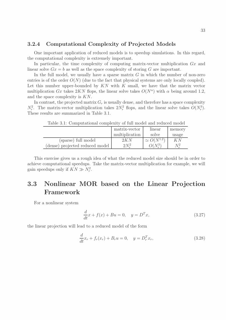
33

3.2.4 Computational Complexity of Projected Models

One important application of reduced models is to speedup simulations. In this regard,the computational complexity is extremely important.

In particular, the time complexity of computing matrix-vector multiplication Gx andlinear solve Gx = b as well as the space complexity of storing G are important.

In the full model, we usually have a sparse matrix G in which the number of non-zeroentries is of the order O(N) (due to the fact that physical systems are only locally coupled).Let this number upper-bounded by KN with K small, we have that the matrix vectormultiplication Gx takes 2KN flops, the linear solve takes O(Nα) with α being around 1.2,and the space complexity is KN .

In contrast, the projected matrixGr is usually dense, and therefore has a space complexityN2

r . The matrix-vector multiplication takes 2N2r flops, and the linear solve takes O(N3

r ).These results are summarized in Table 3.1.

Table 3.1: Computational complexity of full model and reduced model

matrix-vector linear memorymultiplication solve usage

(sparse) full model 2KN ≃ O(N1.2) KN(dense) projected reduced model 2N2

r O(N3r ) N2

r

This exercise gives us a rough idea of what the reduced model size should be in order toachieve computational speedups. Take the matrix-vector multiplication for example, we willgain speedups only if KN ≫ N2

r .

3.3 Nonlinear MOR based on the Linear Projection

Framework

For a nonlinear system

d

dtx+ f(x) +Bu = 0, y = DTx, (3.27)

the linear projection will lead to a reduced model of the form

d

dtxr + fr(xr) +Bru = 0, y = DT

r xr, (3.28)

34

where

fr(xr) = W Tf(V xr),

Br = W TB,

Dr = V TD.

(3.29)

3.3.1 Set of Projected Reduced Models

Similar the the linear case, the nonlinear reduced model is in the set Mr,NL of all dif-ferential equations in the form of (3.28), and is determined by all choices of (fr(·), Br, Dr),i.e.,

Mr,NL =

d

dtxr + fr(xr) +Bru = 0, y = DT

r xr

∣

∣

∣

∣

fr : RNr → R

Nr , Br ∈ RNr×Ni , Dr ∈ R

Nr×No

.

(3.30)In contrast, the reduced model in the set of projected modelsMr,V , (3.28) with (3.29),

is determined by all pairs of (V,W ) where W T = (V TV )−1V T , i.e.,

Mr,V =

d

dtxr +W Tf(V xr) +W TBu = 0, y = DTV xr

∣

∣

∣

∣

V ∈ RN×Nr ,W T = (V TV )−1V T

.

(3.31)Furthermore, instead of choosing a projection matrix V , but choosing a Nr-dimensional

subspace V in RN , we have

Mr,V =

d

dtxr +W Tf(V xr) +W TBu = 0, y = DTV xr

∣

∣

∣

∣

V ∈ Grass(Nr, N),W T = (V TV )−1V T

.

(3.32)We hope to answer the same two questions we have addressed in the linear case:

1. What is the degree of freedom in choosing a nonlinear reduced model?

2. Are the projected models good candidates to use in MOR (i.e., do they encompass allpossible nonlinear reduced models; if not what subset of models can be represented)?

However, we are not able to give exact answers, due to the lack of canonical form andthe lack of analytical response functions such as transfer functions.

3.3.2 Computational Complexity of Projected Models

In the full model, the nonlinear function f(x) is “sparse”, meaning that each elementfi(x) depends on only a few variables (K of them), and only takes at maximum L flops foreach nonlinear kernel. Therefore, the function evaluation takes NKL flops, and the Jacobianmatrix has only NK non-zero elements and is sparse.

35

In contrast, the projected nonlinear function fr(xr) is “dense”, meaning that fr,i(xr)depends on all variables in xr. Without any symbolic simplification, fr(xr) can be computedby computing x = V xr, f(x) and W Tf(x) sequentially, resulting in NKL + 2NNr flops.This is always larger than the that of the full model.

On the other hand, unlike the LTI case where W TGV can be pre-computed and stored inthe reduced model, there is no simple way to store a nonlinear function W Tf(V ·), thereforeresulting in difficulties of storing the reduced model.

We will discuss methods to handle such difficulties in Section 4.7.

36

Chapter 4

Nonlinear Projection Framework forModel Order Reduction

While the linear projection framework works very well for reducing LTI models, it is lessso for reducing nonlinear models. In this chapter, we study how linear projections can failin nonlinear MOR, from which we motivate and propose the nonlinear projection frameworkthat provides an elegant alternative for nonlinear MOR. We analyze each component inthis framework (e.g., choosing manifolds and projections), and present general guidelines ofderiving nonlinear projected reduced models under this framework.

4.1 Motivation

The linear projection framework amounts to finding two subspaces V = span(V ) andW = span(W ) and imposing constraints x ∈ V, r ⊥ W. Loosely speaking, we want to findtwo subspace V and W so that the solution of the full model stay very close to V and thatthe residual of the reduced model solution is orthogonal to W.

Example 4.1.1 (A simple LTI system) Consider a simple LTI system defined by

d

dt

x1

x2

x3

=

−10 1 11 −1 01 0 −1

x1

x2

x3

+

100

u(t), (4.1)

where x = [x1, x2, x3]T are the three state variables, u(t) is the input.

We perform a series of simulations of (4.1) by applying several random sinusoidal inputs.The trajectories of x(t) and dx

dt(t) are plotted in Fig. 4.1(a) and Fig. 4.1(b), respectively. In

this case, the trajectories lie exactly on a 2-dimensional linear subspace, and we expect thatthe MOR algorithm is able to identify that linear subspace.

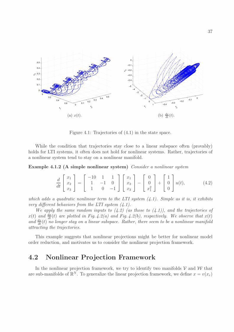
37

0

0.2

0.4

0.60

0.10.2

0.30.4

0.5

0

0.1

0.2

0.3

0.4

0.5

x2x

1

x3

(a) x(t).

−5

−4

−3

−2

−1

0

1 −0.4−0.3

−0.2−0.1

0

−0.4

−0.3

−0.2

−0.1

0

x2

x1

x3

(b) dxdt(t).

Figure 4.1: Trajectories of (4.1) in the state space.

While the condition that trajectories stay close to a linear subspace often (provably)holds for LTI systems, it often does not hold for nonlinear systems. Rather, trajectories ofa nonlinear system tend to stay on a nonlinear manifold.

Example 4.1.2 (A simple nonlinear system) Consider a nonlinear system

d

dt

x1

x2

x3

=

−10 1 11 −1 01 0 −1

x1

x2

x3

−

00x21

+

100

u(t), (4.2)

which adds a quadratic nonlinear term to the LTI system (4.1). Simple as it is, it exhibitsvery different behaviors from the LTI system (4.1).

We apply the same random inputs to (4.2) (as those to (4.1)), and the trajectories ofx(t) and dx

dt(t) are plotted in Fig. 4.2(a) and Fig. 4.2(b), respectively. We observe that x(t)

and dxdt(t) no longer stay on a linear subspace. Rather, there seem to be a nonlinear manifold

attracting the trajectories.

This example suggests that nonlinear projections might be better for nonlinear modelorder reduction, and motivates us to consider the nonlinear projection framework.

4.2 Nonlinear Projection Framework

In the nonlinear projection framework, we try to identify two manifolds V and W thatare sub-manifolds of RN . To generalize the linear projection framework, we define x = v(xr)

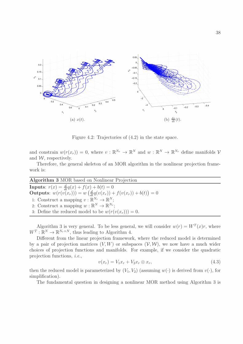
38

0

0.2

0.4

0.60

0.10.2

0.30.4

0.5

0

0.05

0.1

0.15

0.2

x2x

1

x3

(a) x(t).

−4

−2

0

−0.4−0.3

−0.2−0.1

0

−0.2

−0.15

−0.1

−0.05

0

0.05

x2

x1

x3

(b) dxdt(t).

Figure 4.2: Trajectories of (4.2) in the state space.

and constrain w(r(xr)) = 0, where v : RNr → RN and w : RN → R

Nr define manifolds Vand W, respectively.

Therefore, the general skeleton of an MOR algorithm in the nonlinear projection frame-work is:

Algorithm 3 MOR based on Nonlinear Projection

Inputs: r(x) = ddtq(x) + f(x) + b(t) = 0

Outputs: w(r(v(xr))) = w(

ddtq(v(xr)) + f(v(xr)) + b(t)

)

= 0

1: Construct a mapping v : RNr → RN ;

2: Construct a mapping w : RN → RNr ;

3: Define the reduced model to be w(r(v(xr))) = 0.

Algorithm 3 is very general. To be less general, we will consider w(r) = W T (x)r, whereW T : RN → R

Nr×N , thus leading to Algorithm 4.Different from the linear projection framework, where the reduced model is determined

by a pair of projection matrices (V,W ) or subspaces (V,W), we now have a much widerchoices of projection functions and manifolds. For example, if we consider the quadraticprojection functions, i.e.,

v(xr) = V1xr + V2xr ⊗ xr, (4.3)

then the reduced model is parameterized by (V1, V2) (assuming w(·) is derived from v(·), forsimplification).

The fundamental question in designing a nonlinear MOR method using Algorithm 3 is

39

Algorithm 4 MOR based on Nonlinear Projection with w(r) = W T (x)r

Inputs: ddtq(x) + f(x) + b(t) = 0

Outputs: W T (v(xr))(

ddtq(v(xr)) + f(v(xr)) + b(t)

)

= 0

1: Construct a mapping v : RNr → RN ;

2: Construct a mapping w(r) = W T (x)r where W T : RN → RNr×N ;

3: Define w(r(v(xr))) = 0.

how to identify manifolds V and W. Similar to LTI MOR, the manifold to be used in MORdepends on the reduction criterion F (·, ·), G(·, ·) and H(·, ·) in (2.1). In this section, ratherthan being very general to answer this question, we study some candidate manifolds, andtry to draw insights and conclusions.

The notations and simplifications that will be used in this section include:

1. We consider reducing ODE models, instead of DAE models, i.e.,

d

dtx = f(x) +Bu. (4.4)

2. Suppose x ∈ V, i.e., x = v(xr). We denote V (x) for all x = v(xr) by

V (x) =dv

dxr

∣

∣

∣

∣

x=v(xr)

. (4.5)

3. Define W T (x) = W T (v(xr)) such that

W T (v(xr))V (v(xr)) = I. (4.6)

In this case, the reduced model is simplified to

d

dtxr = fr(xr) +Br(xr)u, (4.7)

wherefr(xr) = W T (v(xr))f(v(xr)), Br(xr) = W T (v(xr))B. (4.8)

Therefore, W is determined by V.

4.3 Manifold Integrating Local Krylov Subspaces

The first candidate manifold we study is the one that “integrates” local Krylov subspaces.For nonlinear systems, properties are often described in terms of linearized systems. For

example, TPWL [2] tries to find a linear subspace which covers the local Krylov subspaces

40

around all expansion points. The linear subspace, however, is likely to grow very quickly asthe number of expansion points increases.

In order to avoid the growth of the order of reduced models due to the inclusion of manylinear subspaces, we expect to construct a manifold V so that at each point x ∈ V, thetangent space around x, TxV matches the local Krylov subspace of the linearized system atx.

In another word, the mapping v : RNr → RN should satisfy

span(V (x)) = span

(

∂v

∂xr

∣

∣

∣

∣

x=v(xr)

)

= KNr ,x, (4.9)

where KNr,x is the Nr-dimensional Krylov subspace of the linearized system around x. Sucha manifold is called an integral manifold.

To see why the manifold satisfying (4.9) is useful, we show that responses of the fulllinearized model and the reduced linearized model are closely related.

By linearizing (4.4) around xi ∈ RN , (i.e., let x = xi + ∆x, with higher-order terms of

∆x truncated), we obtain

d

dt∆x = G(xi)∆x+ f(xi) +Bu, (4.10)

where

G(x) =∂f

∂x(x). (4.11)

In contrast, the linearized model of (4.7) around xr,i

d

dt∆xr = Gr(xr,i)∆xr + fr(xr,i) +Br(xr,i)u, (4.12)

where1

Gr(xr) =∂

∂xr

[

W T (v(xr))[f(v(xr)) +Bu]]

= W T (v(xr))G(x)|x=v(xr)V (v(xr)) +∂W T (v(xr))

∂xr· (f(v(x)) +Bu),

Br(xr) =∂

∂u

[

W T (v(xr))[f(v(xr)) +Bu]]

= W T (v(xr))B.

(4.13)

To compare (4.10) with (4.12), let xi = v(xr,i), and consider xi that is an equilibrium

1Note: ∂WT (x)∂x

is a 3-dimensional tensor, and therefore the notation ∂WT (v(xr))∂xr

· (f(v(x)) +Bu) denotesa matrix of size Nr ×Nr.

41

point, i.e.,f(xi) +BuDC = 0, (4.14)

where uDC is a DC (constant) input.Given (4.14), the second part of Gr(xr) in (4.13) vanishes, and therefore (4.12) is a linear

reduced model of (4.10) with projection matrices V (v(xr)) andW (v(xr)). Furthermore, sincespan(V (v(xr))) = KNr,v(xr), the first Nr moments of the transfer function of (4.12) matchthose of (4.10).

4.4 Existence of an Integral Manifold

The manifold defined in the last section would be useful for model reduction. However,the key question is: can we find an Nr-dimensional manifold satisfying conditions (4.9)?Unfortunately, generally the answer is no. To show that, we resort to a fundamental resultin differential geometry [73, 112, 113], the Frobenius theorem.

To explain the result of Frobenius theorem, we introduce a few terminologies in differentialgeometry2:

1. Let X denote a manifold.

2. A distribution on X is a map ∆ which assigns to each point p in X a subspace ofthe tangent space at this point, i.e.,

p ∈ X → ∆(p) ∈ TpX. (4.15)

3. A foliation Sαα∈A of X of dimension k is a partition

X =⋃

α∈A

Sα (4.16)

of X into disjoint connected sub-manifolds Sα, called leaves, which has the followingproperty: for any p ∈ X there exists a neighborhood U of p and a diffeomorphismΦ : U → V ⊂ R

N onto an open subset V such that

Φ((U⋂

Sα)cc) = p = (x1, · · · , xN) ∈ V |xk+1 = ck+1α , · · · , xN = cNα , (4.17)

where Pcc denotes a connected component of the set P .

4. A distribution of constant dimension p → ∆(p) on X is integrable if there exists a

2For self-contained ness, we provide a short introduction to differential geometry that is relevant to ourdiscussion in Appendix Chapter A.

42

foliation Sαα∈A on X such that for any p ∈ X ,

TpS = ∆(p), (4.18)

where S is the leaf passing through p.

This series of rather semi-formal definitions leads to the following important result: thereexists a sub-manifold S that satisfies TpS = ∆(p) for some distribution ∆ if the distribution∆ is integrable.

Furthermore, the other important result that makes us able to tell the integrability of adistribution ∆ is given by the Frobenius theorem.

Theorem 4.4.1 ((Global) Frobenius theorem) A smooth distribution ∆ of constant di-mension is integrable if and only if it is involutive. The integral foliation of ∆ is the partitionof a manifold X into orbits of the family of vector fields g|g ∈ ∆.

Theorem 4.4.2 ((Local) Frobenius theorem) A distribution ∆ = span(g1, · · · , gk) ofconstant dimension k is involutive if and only if there exists a diffeomorphism ϕ such thatif ξ = ϕ(x), then

(Dϕ∆)(ξ) = span(Dϕg1, · · · , Dϕgk) = span

(

∂

∂ξ1, · · · ∂

∂ξk

)

. (4.19)

In Theorem 4.4.1 and 4.4.2, we encounter the definition of the involutivity of a distri-bution.

Definition 4.4.1 (Involutivity of a distribution) A distribution ∆ is involutive if forany vector fields f, g ∈ ∆, their Lie bracket is also in ∆, i.e., [f, g] ∈ ∆.

Definition 4.4.2 (Lie bracket (coordinate-dependent)) The Lie bracket of two vectorfields f and g, denoted by [f, g], is

[f, g] =∂g

∂x(x)f(x)− ∂f

∂x(x)g(x). (4.20)

From the above discussion and theorems, we conclude:

1. We can define a sub-manifold by defining an integrable distribution ∆ that specifiesthe tangent space at each point on the sub-manifold.

2. We can check the integrability of a distribution by checking its involutivity.

3. We can check the involutivity of a distribution by checking whether the Lie bracket oftwo vector fields in the distribution is still in the distribution.

43

In Section 4.3, we have specified the distribution ∆ to be the one assigning Krylov sub-spaces to each point on the manifold, i.e.,

∆K(x) , span(KNr) = span(G−1(x)B, · · · , G−Nr(x)B), ∀x = v(xr), xr ∈ R

Nr . (4.21)

One distribution that satisfies (4.21) is

∆K(x) , span(KNr) = span(G−1(x)B, · · · , G−Nr(x)B), ∀x ∈ R

N . (4.22)

Unfortunately, this distribution is generally not involutive, and therefore such amanifold may not exist. A counter-example can be constructed as follows:

Example 4.4.3 Consider a linearized model in the form of

A(x)dx

dt+ x+Bu = 0, (4.23)

where A(x) ∈ RN×N and B ∈ R

N×1.They Krylov basis of (4.23) is

V (x) = [A(x)B,A(x)2B, · · · , A(x)kB]. (4.24)

Let N = 3, Nr = 2. Let A(x) be the Jacobian of a nonlinear function g(x), given by

g(x) =

x1x3

x2x3

x1

, A(x) =∂g

∂x(x) =

x3 0 x1

0 x3 x2

1 0 0

, (4.25)

and let B be a constant vector

B =

100

. (4.26)

Therefore, the two-dimensional Krylov subspace is the span of v1 = A(x)B, v2 = A(x)2B,where

v1(x) =

x3

01

, v2(x) =

x23 + x1

x2

x3

. (4.27)

The Lie bracket [v1, v2] is

[v1, v2] =∂v2∂x

v1 −∂v1∂x

v2 =

2x3

01

. (4.28)

44

When x1 = 1, x2 = 1, x3 = 1, we have

v1(x) =

101

, v2(x) =

211

, [v1, v2] =

201

/∈ span(v1, v2), (4.29)

and therefore ∆ defined by (4.21) is not involutive.

4.5 Involutive DistributionMatching Krylov Subspaces

While the distribution defined by (4.21) is typically not involutive, we may induce aninvolutive distribution from it. Given a set of analytical vector fields fu, ∆ = span(fu),we may define

L(p) = spang(p)|g ∈ Liefu (4.30)

where Liefu is the smallest family of vector fields that contains fu and is closed undertaking linear combinations and Lie bracket (or the Lie algebra of fu).

According to corollary A.7.2, the orbit of (p, fu) defines a sub-manifold whose tangentspace

TpX = L(p). (4.31)

In another word, L(p) defines an involutive distribution that covers the subspace definedby ∆ at each point p. Therefore, L(p) corresponds to a well-defined sub-manifold.

In order to compute L(p), we can start with L(p) = span(fu) = ∆, and then iterativelyadd Lie brackets of generator functions in L(p) into L(p) until L(p) is involutive.

The possible caveat of this approach is that there does not seem to have any bound ofthe dimension of L(p). Therefore, even in the case where we want to match all 2-dimensionalKrylov subspaces, L(p) may end up being of a large dimension, making the manifold not soefficient in preserving accuracy of linearized models.

4.6 Constructing Integral Manifolds

We have seen that ∆K in (4.21) is generally not involutive, and ∆K-induced L(p) is involu-tive but may be of large dimension. However, the discussion gives us a better understandingon how we may define a manifold (more precisely, a sub-manifold in R

N ):

1. We may define an involutive distribution, or equivalently, its generator functions, fromwhich a sub-manifold can be derived;

2. We may directly define the projection function x = v(xr) that specifies the manifoldV, and derive its tangent spaces V (x) = ∂v

∂xr(v(xr)).

45

In this section, we consider several ways to construct integral manifolds, and considerspecial kinds of distributions/manifolds that may be analyzed or computed efficiently.

In the following discussion, we assume the projections x = v(xr) and xr = w(x) suchthat xr = w(v(xr)) for all xr. Note that this definition leads to the reduced model

dxr

dt=

dw

dx

dx

dt=

dw

dx(v(xr))(f(v(xr)) +Bu), (4.32)

which is the same as that in (4.7), and in Algorithm 4.We denote ∂v

∂xr(xr) as V (xr), V (w(x)) as V (x)3, ∂w

∂x(x) as W T (x), and W T (v(xr)) as

W T (xr).Note that x = v(xr) has N equations, and xr = w(x) has Nr equations. Therefore, x =

v(xr) specifies all the points on a manifold, while xr = w(x) specifies equivalent classes, i.e.,it specifies points x ∈ R

N that map/project to the same xr. Equivalently, xr = w(x) definesthe projection from x to xr on the manifold (corresponding to v(xr) in R

N ). Therefore, theassumption xr = w(v(xr)) simply states that the projection of a point on the manifold isthe same point.

Example 4.6.1 1. [x1, x2, x3] = [xr, xr, xr] specifies a one-dimensional manifold (a line)in R

3.

2. xr = x21 +x2

2+x23 defines equivalent points in R

3 being points on spheres of radius√xr

(xr ≥ 0).

4.6.1 Involutivity Constraints

To enforce the involutivity of a distribution span(V (x)) = span([v1, · · · , vNr]) so that it

corresponds to an integral manifold, we have involutivity constraints

[vi, vj ] ∈ span(V (x)), ∀i, j, i 6= j. (4.33)

Using coordinate-dependent definition of the Lie bracket, we have

[vi, vj] =∂vj∂x

vi −∂vi∂x

vj ∈ span(V (x)), ∀i, j, i 6= j. (4.34)

To simplify (4.34), we note that from the proof of the Frobineous theorem, if span(V (x))is involutive, then there exists a commuting basis of generators for span(V (x)). Therefore,without loss of generality, we assume that vi(x) and vj(x) are commuting, leading to algebraicequations

[vi, vj] =∂vj∂x

vi −∂vi∂x

vj = 0, ∀i, j, i 6= j. (4.35)

3This definition is an extension to the one in (4.5) for x /∈ V , with the assumption that w(v(xr)) = xr.

46

For each pair (i, j), (4.35) correspond to N equations. Since there are 12Nr(Nr − 1) (i, j)

pairs, the involutivity constraints consist of 12Nr(Nr − 1)N equations.

4.6.2 Method 1

In method 1, we directly construct v(·) and w(·) with the constraint

xr = w(v(xr)), (4.36)

which states that the projection from xr to x and then x to xr leads to the same point onthe manifold.

With (4.36), we may immediately prove that for any x = v(xr), the distribution definedby span(V (x)) is involutive, and that the basis given by V (x) is commuting.

Theorem 4.6.2 If xr = w(v(xr)), then for all x = v(xr), [vi(x), vj(x)] = 0 for all i, j, i 6= j.

Proof By definition,

vi(x) =∂v

∂xr,i

∣

∣

∣

∣

xr=w(x)

, vj(x) =∂v

∂xr,j

∣

∣

∣

∣

xr=w(x)

. (4.37)

Therefore,

[vi, vj ] =∂vj∂x

vi −∂vi∂x

vj

=∂2v

∂xr∂xr,j

∂w

∂x

∂v

∂xr,i− ∂2v

∂xr∂xr,i

∂w

∂x

∂v

∂xr,j.

(4.38)

Take the derivative of xr = w(v(xr)) with respect to xr, we obtain

I =∂w

∂x

∂v

∂xr

, ∀x = v(xr), (4.39)

and therefore∂w

∂x

∂v

∂xr,i= ei. (4.40)

47

Therefore, (4.38) simplifies to

[vi, vj] =∂2v

∂xr∂xr,jei −

∂2v

∂xr∂xr,iej

=∂

∂xr,j

(

∂v

∂xr,i

)

− ∂

∂xr,i

(

∂v

∂xr,j

)

= 0

(4.41)

While we haven’t shown that V (x) is involutive for all x ∈ RN , we see that by definition,

we have an integral manifold V that satisfies TxrV = span(V (x)). Therefore, the projections

v(·) and w(·) lead to a well-defined integral manifold.However, in practice, it can still be hard or impossible to construct analytical expressions

of the nonlinear functions v(·) and w(·) that satisfy (4.36), except for a few special cases.

Example 4.6.3 Consider linear functions

x = v(xr) = x0 + V xr, xr = w(x) = xr,0 +W Tx, (4.42)

where x0 ∈ RN , xr,0 ∈ R

Nr , V ∈ RN×Nr and W ∈ R

N×Nr .The condition (4.36) for (4.42) translates to

xr = xr,0 +W T (x0 + V xr) = xr,0 +W Tx0 +W TV xr (4.43)

For (4.43) to hold for all xr, we must have

xr,0 +W Tx0 = 0,

W TV = I.(4.44)

Therefore, given V, x0, one of the many choices of W T and xr,0 is

W T = (V TV )−1V T ,

xr,0 = −W Tx0.(4.45)

Example 4.6.4 Consider a nonlinear function v(·) and a linear function w(·):

x = v(xr) = [V, Vg][xr; g(xr)] = V xr + Vgg(xr), xr = w(x) = W Tx, (4.46)

where g(xr) ∈ Rk, V ∈ R

N×Nr , Vg ∈ RN×k, W T ∈ R

Nr×N , with k being the number ofnonlinear functions in g(xr).

48

In this case, (4.36) becomes

xr = W T (V xr + Vgg(xr)). (4.47)

Define W such that W TV = I4. We obtain

W TVgg(xr) = 0. (4.48)

A sufficient condition for (4.48) to hold is W TVg = 0, or in another word, columns of Vg

are orthogonal to columns of W .For example, consider

x = v(xr) = [xr,1, xr,2, xr,1xr,2], xr = w(x) = W Tx = [x1, x2]. (4.49)

In (4.49), we define the manifold by v(·) which is the surface defined by x1 = xr,1, x2 =xr,2, x3 = xr,1xr,2. On the other hand, we define the projection of each point x to the manifoldby w(·): for any point (x1, x2, x3), the projection leads to the point v(w(x)) = (x1, x2, x1x2).

(4.48) corresponds to V = W = [I2; 0], Vg = e3. As a result, W TVg = 0. Therefore, V (x)defines an integral manifold.

Note also that in this example, the manifold (defined by v(·)) is nonlinear, but the pro-jection (defined by w(·)) is linear.

Example 4.6.5 Consider a linear function v(·) and a nonlinear function w(·):

x = v(xr) = V xr, xr = w(x) = W Tx+W Tg g(x). (4.50)

In this case, (4.36) becomes

xr = W TV xr +W Tg g(V xr). (4.51)

Again, if we define W such that W TV = I5, we have

W Tg g(V xr) = 0. (4.52)

To simplify the problem, we further assume g(x) are quadratic functions, i.e., g(x) =x⊗ x. Then,

W Tg (V xr)⊗ (V xr) = W T

g (V ⊗ V )(xr ⊗ xr) = 0, (4.53)

for which a sufficient condition is

W Tg (V ⊗ V ) = 0. (4.54)

4This might not be the best choice, though.5This might also not be a good choice.

49

For example, considerV = [1; 0; 0], W = [1; 0; 0]. (4.55)

We then haveV ⊗ V = [1; 0; 0; 0; 0; 0; 0; 0; 0], (4.56)

and a valid choice of W Tg is

W Tg = [0, 0, 0, 0, 0, 0, 0, 0, 1]. (4.57)

These choices correspond to

x = v(xr) = [xr; 0; 0]

xr = w(x) = x1 + x23

(4.58)

In this case, the manifold is the x1 axis (a linear subspace), but the projection of anypoint to the x1 axis is the parabola x1 + x2

3 = 0 (nonlinear).

4.6.3 Method 2

In method 2, we start with an involutive and commuting basis V (x), from which weinduce the mapping v(·) by solving

dx

dxr= V (x). (4.59)

Specifically, the commuting basis V = [v1, · · · , vNr] provides a natural definition of v(·) that

also serves as a parameterization of the manifold

v : (xr,1, · · · , xr,Nr) 7→ exp(xr,1v1) · · · exp(xr,Nr

vNr), (4.60)

where exp(xr,ivi) is the solution todx

dxr,i

= vi(x). (4.61)

Since columns of V (x) commute, we can change the order of the integration withoutchanging the mapping. With V (x), we can also induce a W (x) by ensuring W T (x)V (x) = I.

In this method, we have not explicitly defined the projection xr = w(x) although it may

be induced by solving dw(x)dx

= W T (x). However, we do not have to compute w(x) for thepurpose of reduced order modeling – W T (x) alone is enough to construct a reduced ordermodel.

One way to find such a V (x) that also preserves system responses (such as momentsof linearized models) is to start with a non-involutive and non-commuting “accurate” basis

50

(e.g., the Krylov basis), and then try to find a “closest” distribution to it.Another way is to consider specific basis functions, and derive simpler conditions for

involutivity and commutativity.

Example 4.6.6 Consider V (x) = [v1, · · · , vNr] where vi(x) is in the form of

vi(x) = Aix+ bi, i = 1, · · · , Nr, (4.62)

where Ai ∈ RN×N and bi ∈ R

N×1.Applying the involutivity constraint in (4.35) on the pair (vi, vj), we obtain

[vi, vj ] = Aj(Aix+ bi)− Ai(Ajx+ bj)

= (AjAi −AiAj)x+ (Ajbi − Aibj) = 0.(4.63)

In order for (4.63) to be equal to 0 for all x, we must have

AjAi −AiAj = 0,

Ajbi − Aibj = 0.(4.64)

For simplicity, considerAi = UΛiU

−1, (4.65)

where columns of U are the eigenvalues of A and Λi is diagonal with eigenvalues of Ai onthe diagonal.

Ai’s defined by (4.65) are commuting:

AiAj = UΛiU−1UΛjU

−1 = UΛiΛjU−1 = UΛjΛiU

−1 = UΛjU−1UΛiU

−1 = AjAi. (4.66)

We also obtain bj in terms of bi:

bj = A−1i Ajbi = UΛ−1

i U−1UΛjU−1bi = UΛ−1

i ΛjU−1bi. (4.67)

4.6.4 Method 3

In method 3, we start with an arbitrary distribution defined by U(x) that may be non-involutive or non-commuting. However, we can still define a mapping v : xr 7→ x by

v : (xr,1, · · · , xr,Nr) 7→ exp(xr,Nr

uNr) · · · exp(xr,1u1). (4.68)

In another word, the mapping is obtained by integrating

dx

dxr,i

= ui(x) (4.69)

51

in a specified order (i = 1, · · · , Nr).From this mapping, we may then derive the distribution

V (x) =dv(xr)

dxr

∣

∣

∣

∣

xr=w(x)

, (4.70)

by defining a projection xr = w(x).In fact, the ManiMOR approach to be introduced in Chapter 5 uses this method to

construct the manifold.

4.7 Reduced Model Data Structure and Computation

The storage of mapping functions x = v(xr), xr = w(x), or the associated distributionsV (x) and W T (x) can be difficult and expensive. Moreover, to compute the reduced model,we ultimately need to store and compute

fr(xr) = W T (v(xr))f(v(xr)), (4.71)

which may be even more complicated.

4.7.1 Symbolic/Analytical Representation

If v(xr), w(x) have analytical expressions, we may simply store their symbolic expression.In particular, some special functions even have a matrix representation, such as quadraticfunctions

v(xr) = G1xr +G2xr ⊗ xr, (4.72)

for which we may just store the matrices G1 and G2.Moreover, analytical expressions of v(·) and w(·) may help simplify (4.71). In the linear

projection framework, we havefr(xr) = W TGV xr, (4.73)

where W TGV ∈ RNr×Nr can be precomputed and stored, and is N -independent. We may

do the similar trick in the nonlinear case.

Example 4.7.1 Consider the case where

v(xr) = V1xr + V2xr ⊗ xr,

f(x) = G1x+G2x⊗ x,

W T (x) = W T .

(4.74)

52

We obtain

fr(xr) =W T (G1(V1xr + V2xr ⊗ xr) +G2(V1xr + V2xr ⊗ xr)⊗ (V1xr + V2xr ⊗ xr))

=W TG1V1xr +W TG1V2xr ⊗ xr

+W TG2[(V1 ⊗ V1)(xr ⊗ xr) + (V1 ⊗ V2)(xr ⊗ xr ⊗ xr)

+ (V2 ⊗ V1)(xr ⊗ xr ⊗ xr) + (V2 ⊗ V2)(xr ⊗ xr ⊗ xr ⊗ xr)]

=W TG1V1xr + (W TG1V2 +W TG2(V1 ⊗ V1))(xr ⊗ xr)

+W TG2(V1 ⊗ V2 + V2 ⊗ V1)(xr ⊗ xr ⊗ xr)

+W TG2(V2 ⊗ V2)(xr ⊗ xr ⊗ xr ⊗ xr),

(4.75)

where we only have N-independent matrices to pre-compute and store in the reduced model.

4.7.2 Piecewise Linear Approximation

When no analytical expression is available, we have to use certain approximation for thenonlinear mappings and nonlinear functions. One such approximation is PWL approxima-tion6, i.e., concatenating (interpolating) point-wise linearized functions to obtain a globalfunction.

Approximating mapping functions

In PWL approximation, we assume that, instead of the actual nonlinear function x =v(xr), we are given a few pairs of (xr,i, xi), i = 1, · · · , Ns where Ns is the number of sampleson the manifold. Therefore, we can approximate v(·) by

x =

Ns∑

i=1

Ki(xr)xr,i, (4.76)

where Ki(xr) is a weighting (kernel) function that satisfies

Ki(xr) ≥ 0,Ns∑

i=1

Ki(xr) = 1,

Ki(xr,i) = 1.

(4.77)

When we also have information about the tangent space (e.g., Krylov subspaces) at each

6While the method is traditionally called “piecewise-linear” in MOR community, it is also known as aspecial case of kernel methods.

53

point, i.e.,

Vi =∂v

∂xr

∣

∣

∣

∣

x=v(xr,i)

, (4.78)

we may obtain a better PWL approximation of v(·) by

x =Ns∑

i=1

Ki(xr)(Vi(xr − xr,i) + xi). (4.79)

Similarly, we may approximate w(·) by

xr =

Ns∑

i=1

Ki(xr)(WTi (x− xi) + xi,r). (4.80)

Approximating nonlinear functions

For PWL approximations of nonlinear functions, we assume that we are given fi = f(xi)and Gi =

∂f∂x(xi) for each pair (xi, xr,i). Therefore, the PWL approximation of fr(xr) is

fr(xr) ≃W T (xr)Ns∑

i=1

Ki(xr) (fi +Gi(v(xr)− xi)) . (4.81)

Combine (4.81) and (4.79), we obtain

f(xr) ≃W T (xr)

Ns∑

i=1

Kfi (xr)

(

fi +Gi(

Ns∑

j=1

Kvj (xr)(Vj(xr − xr,j) + xj)− xi)

)

=W T (xr)Ns∑

i=1

Kfi (xr)

(

fi +Kvi (xr)GiVi(xr − xr,j) +Gi(K

vi (xr)xi − xi)

+

Ns∑

j=1,j 6=i

Kvj (xr)(Vj(xr − xr,j) + xj)− xi)

)

.

(4.82)

where Kfi (·) and Kv

i (·) are the weighting functions for f(·) and v(·), respectively.Note that when xr is close to xr,i, Ki(xr) ≃ 1 and Kj(xr) ≃ 0, j 6= i. Therefore, we have

fr(xr) ≃W T (xr)(fi +GiVi(xr − xr,i)). (4.83)

54

Therefore, the PWL approximation of f(·) is often simplified to

fr(xr) ≃W T (xr)

Ns∑

i=1

Ki(xr) (fi +GiVi(xr − xr,i)) , (4.84)

which can be viewed as approximately truncating second-order terms of Kfi (xr)K

vj (xr).

To approximate W T (xr), we differentiate (4.80) and obtain

W T (xr) =∂w

∂x

∣

∣

∣

∣

x=v(xr)

. (4.85)

Similarly, a PWL approximation of W T (xr) is

W T (xr) ≃Ns∑

i=1

wi(xr)WTi . (4.86)

Combine (4.84) with (4.86), and use a simplified PWL approximation, we obtain

fr(xr) ≃Ns∑

i=1

Ki(xr)(WTi fi +W T

i GiVi(xr − xr,i)). (4.87)

Therefore, we can pre-compute and store W Ti fi ∈ R

Nr and W Ti GiVi ∈ R

Nr×Nr in thereduced model. As a result, the computation cost of the reduced model (i.e., (4.87)) isdepends only on Nr and Ns, and is N -independent.

Approximating Jacobians

Taking the derivative of (4.87) with respect to xr, we obtain the Jacobian

∂fr∂xr≃

Ns∑

i=1

Ki(xr)WTi GiVi +

Ns∑

i=1

∂Ki(xr)

∂xr

[

W Ti fi +W T

i GiVi(xr − xr,i)]

. (4.88)

Note that when ∂Ki(xr)∂xr

is small (which is true for xr far away from xi), we can furtherignore the second part in (4.88), and obtain

∂fr∂xr

≃Ns∑

i=1

Ki(xr)WTi GiVi. (4.89)

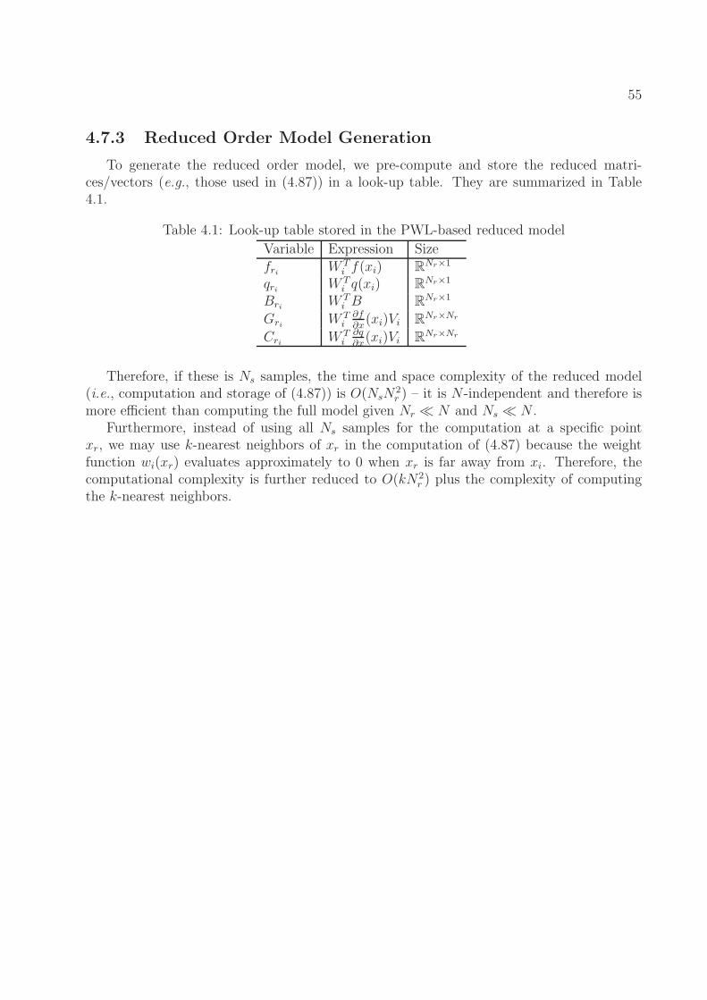
55

4.7.3 Reduced Order Model Generation

To generate the reduced order model, we pre-compute and store the reduced matri-ces/vectors (e.g., those used in (4.87)) in a look-up table. They are summarized in Table4.1.

Table 4.1: Look-up table stored in the PWL-based reduced model

Variable Expression Sizefri W T

i f(xi) RNr×1

qri W Ti q(xi) R

Nr×1

Bri W Ti B R

Nr×1

Gri W Ti

∂f∂x(xi)Vi R

Nr×Nr

Cri W Ti

∂q∂x(xi)Vi R

Nr×Nr

Therefore, if these is Ns samples, the time and space complexity of the reduced model(i.e., computation and storage of (4.87)) is O(NsN

2r ) – it is N -independent and therefore is

more efficient than computing the full model given Nr ≪ N and Ns ≪ N .Furthermore, instead of using all Ns samples for the computation at a specific point

xr, we may use k-nearest neighbors of xr in the computation of (4.87) because the weightfunction wi(xr) evaluates approximately to 0 when xr is far away from xi. Therefore, thecomputational complexity is further reduced to O(kN2

r ) plus the complexity of computingthe k-nearest neighbors.

56

Chapter 5

ManiMOR: General-PurposeNonlinear MOR by Projection ontoManifolds

In this chapter, we present a general-purpose nonlinear MOR technique based on thenonlinear projection framework presented in Chapter 4. The algorithm explicitly constructsand parameterizes a manifold in the state space, and projects the original nonlinear modelto the manifold to obtain a nonlinear reduced order model.

We describe in detail how we construct and parameterize a general-purpose manifoldthat captures typical system responses (such as DC and AC responses). We validate andillustrate the MOR technique using several examples.

5.1 Construction of the Manifold

Many dynamical systems derived from engineering problems work in certain highly con-strained region in the state space, either because the fast dynamics die out very quickly andare not easily observable, or because the systems are designed/engineered to work undercertain mode (e.g., amplifiers are designed to work around a DC steady state / equilibrium,and oscillators are designed to work around a limit cycle). In another word, state variablestypically stay close to the attractors, and that part of the state space covers important dy-namics. In order for the reduced model to reproduce the attractors, a necessary condition isthat the manifold must cover the attractors.

5.1.1 DC Manifold

We first consider the manifold covering equilibria (also known as DC operating points incircuit community) of a system.

57

For the nonlinear system (1.2), the DC equilibria are the solution to

f(x) +Bu = 0, u ∈ [umin, umax], (5.1)

where umin and umax are bounds of the input u according to physical constraints.For simplicity, we consider the case where f(·) is invertible. We consider this assumption

because it is often satisfied in a large number of circuit examples.As a result of this assumption, we have

x = f−1(−Bu), (5.2)

which defines a one-dimensional manifold (parameterized by u) consisting of all DC solutions.This constitutes the first dimension of the manifold, and we call it DC manifold.

Equivalently, the solution of (5.2) can be written as the solution to

∂x

∂u= −∂f

−1

∂b(−Bu)B, x(u = 0) = f−1(0), (5.3)

where ∂f−1

∂b(·) is the Jacobian of f−1(·). (5.3) is obtained by taking the partial derivative of

(5.2) with respect to u.Similarly, we may directly take the partial derivative of (5.1) with respect to u, and

obtain

G(x)∂x

∂u+B = 0, (5.4)

and therefore we can define

v1(x) =∂x

∂u= −G−1(x)B, (5.5)

which associate each point on the DC manifold with its tangent space.The RHS of (5.5) is exactly the direction of the first Krylov vector of the linearized model

around x. Therefore, as proved in [89], at each DC equilibrium, the linearized reduced modelmatches the first moment of the linearized full model.

5.1.2 AC manifold

The AC response is determined by the linearized models around DC solutions. To reducethese linearized models, we may use any LTI MOR method described in Section 2.3.

Specifically, for each linearized model, the first dimension of the reduced subspace isdetermined by the DC manifold, i.e., the first Krylov vector, Krylov-subspace based methodsseem to be appropriate, and can be used to compute the tangent spaces at each point on themanifold.

Using Arnoldi-based method, for example, we have that at each point x, the local linearsubspace, or the tangent space of the manifold, is defined by the column span of a nonlinear

58

projection matrix VNr(x) that satisfies

span(VNr(x)) = span(G−1(x)B,G−2(x)B, · · · , G−Nr(x)B). (5.6)

Because the tangent space around a point x gives a good local approximation of themanifold, the points close to x is, loosely speaking, also on the manifold. Therefore, onemay “grow” the manifold by integrating along the Krylov vectors to obtain the manifold.That is, solving

∂x

∂xr

= VNr(x) (5.7)

to obtain the projection x = v(xr).However, according to the discussion in Section 4.4, in general there may not exist a

solution to (5.7). Nevertheless, we can always ensure that at each point on the DC manifold,(5.7) holds (one example is given in Section 5.1.3. We will call any manifold that satisfiesthis condition an AC manifold, because such manifolds lead to reduced order models thatmatch up to the Nr-th moment of the linearized full models, and therefore the AC responsesare well approximated.

5.1.3 Manifold used in ManiMOR

While we do not have a manifold whose tangent spaces match local Krylov subspaces, wecan construct manifolds that cover DC and AC manifolds. In the following, we provide onesuch solution by constructing parametric equations of the manifold in terms of Nr variablesxr = (xr,1, · · · , xr,Nr

).Let VNr

(x) = [v1(x), · · · , vNr(x)] be the Krylov basis of the linearized system around x,

and let x0 = f−1(0) be the DC solution for u = 0. We “grow” the manifold V starting fromx0:

1. Solve for x = v(xr,1, 0, · · · , 0) by integrating

∂x

∂xr,1

= v1(x), x(0) = x0. (5.8)

2. Solve for x = v(xr,1, xr,2, 0, · · · , 0) by integrating

∂x

∂xr,2= v2(x), x(0) = x(xr,1, 0, · · · , 0). (5.9)

3. · · ·

59

4. Solve for x = v(xr,1, xr,2, · · · , xr,Nr) by integrating

∂x

∂xr,Nr

= vNr(x), x(0) = x(xr,1, · · · , xr,Nr−1, 0). (5.10)

In short, the resulting projection function can then be written as

x = v(xr) = exp(VNr(x)xr) = exp(vNr

(x)xr,Nr) · · · exp(v1(x)xr,1). (5.11)

In another word, the manifold is composed of points that are solutions of (5.11).The rationale behind the construction of such a manifold is that at a point x in the

state space, the state variable can move in N independent directions, corresponding to Nmodes which are approximated by the N Krylov basis vectors. Ignoring N − Nr “fast”modes, the state variable will first move along the Nr-th direction (the fastest remainingmode), and then the (Nr − 1)-th direction (the second fastest remaining mode), and so on.In the end, it moves along the first direction (the slowest mode). Therefore, at each point onthe Nr-dimensional manifold, we only guarantee that vNr

(x) is covered by the local tangentspace.

This leads to the conclusion that at each point on the k-dimensional manifold, the localtangent space covers span(vk(x), · · · , vNr

(x)). In particular, at each DC equilibrium, thelocal tangent space covers the Krylov subspace of the linearized model. Therefore, theresulting nonlinear model covers the DC and AC manifolds.

5.2 Parameterization

(5.11) gives a straightforward parameterization of the manifold using xr.While the order of the integration from (5.8) to (5.10) is extremely important, we may

change the magnitude of each Krylov vector without changing the manifold. Hence, we mayobtain many parameterizations of the same manifold. This can be seen from the followingtheorem.

Theorem 5.2.1 Suppose x(t) and x(τ) are the solutions to

d

dtx(t) = g(x(t)) (5.12)

andd

dτx(τ) = σ′(τ)g(x(τ)), (5.13)

respectively, where t = σ(τ) is a function of τ , and g(·) is Lipschitz. Then x(t) and x(τ)define the same points in the state space, i.e.∀t, ∃t, such that x(t) = x(t).

60

Proof Since t = σ(τ), we havedt = σ′(τ)dτ (5.14)

Definex(τ) ≡ x(t) = x(σ(τ)). (5.15)

Therefore,d

dτx(τ) =

dx(τ)

dt

dt

dτ= g(x(t))σ′(τ) = g(x(τ))σ′(τ), (5.16)

i.e.,d

dτx(τ) = σ′(τ)g(x(τ)). (5.17)

According to the existence and uniqueness theorem for ordinary differential equations,x(t) and x(τ) are the unique solutions to (5.12) and (5.17), respectively.

Therefore, x(t) and x(t) define the same points in the state space.

Based on theorem 5.2.1, the following corollary follows.

Corollary 5.2.2 The solutions to the normalized integral curve equation

∂x

∂xr,i

=vi(x)

||vi(x)||(5.18)

define the same trajectory as the solutions to the regular integral curve equation

∂x

∂xr,i

= vi(x). (5.19)

Proof Suppose the solutions to (5.19) and (5.18) are x(t) and x(t), respectively. Let

t = σ(t) =

∫ t

0

1

||vi(x(µ))||dµ. (5.20)

By theorem 5.2.1, x(t) and x(t) span the same state space.

From the above discussion, we conclude that different choices of σ(t) leads to differentparameterizations of the manifold. Nevertheless, they all define the same manifold. There-fore, we may define σ(t) to obtain better numerical accuracy in computing the manifold andthe projection function.

61

5.3 Projection Functions and Matrices

To connect ManiMOR to the nonlinear projection framework, we examine the projectionfunctions x = v(xr), xr = w(x), and the projection matrices V (xr) andW T (x) in ManiMOR.

Essentially, we have used method 3 from Section 4.6.4 in ManiMOR to derive the pro-jections. In Section 4.6.4, v(xr) is given by (4.68), from which we may derive V (xr) by(4.70). With V (xr), we may define W T (xr) such that W T (xr)V (xr) = I, e.g., by W T (xr) =(V T (xr)V (xr))

−1V T (xr).

5.3.1 Numerical Computation

It can be very expensive to use (4.68), or (5.11), to compute the projection functions andthe reduced nonlinear models, because they themselves involve solving a series of differentialequations.

For example, to compute V (x) = ∂x∂xr

, we have to solve

∂x

∂xr,Nr

= vNr(x),

dx

dxr,Nr−1=

∂x

∂x0,xr,Nr−1

vNr−1(x),dx

dxr,Nr−2=

∂x

∂x0,xr,Nr−2

vNr−2(x), · · · ,

(5.21)where x0,xr,i

= x(xr,1, · · · , xr,i, 0, · · · , 0), and the computation of RHS in (5.21) involvesexpensive transient sensitivity analysis.

To alleviate the computational cost of the reduced model, we employ the piece-wise linearapproximation method described in Section 4.7.2 that makes the time and space complexityO(NsN

2r ).

5.4 Summary and Algorithm

As a summary, we present the complete ManiMOR algorithm in Algorithm 5.

Algorithm 5 ManiMOR

Inputs: The full model dxdt

= f(x) +Bu. The reduced order model size Nr.Outputs: dxr

dt= fr(xr) +Bru. A look-up table storing discrete points of x, xr, fr, Br, etc..

1: Solve (4.68) for discrete points on the manifold and its parameterization (xi, xr,i).2: For each xi, compute V (xr) by (4.70), and W T (xr) by (V T (xr)V (xr))

−1V T (xr).3: Compute fr,i, qr,i, Gr,i, Cr,i, Br as described in Section 4.7.2.4: Store fr,i, qr,i, Gr,i, Cr,i, Br in a look-up table.

62

5.4.1 Connections to Previous Methods

Connection to Trajectory-Based Methods

In trajectory-based methods, the trajectories are sampled to identify the region in thestate space where main dynamics of the system evolve. However, trajectory-based methodsembeds these trajectories in a linear subspace, instead of a manifold as is done in ManiMOR.This is the key difference between ManiMOR and trajectory-based methods.

Because of this key difference, trajectory-based methods usually generate a model ofmuch larger size than that of ManiMOR. The simplest example is a nonlinear system whichhas different AC modes (corresponding to local subspaces) when operating under differentDC equilibria. Suppose that the dynamics of each linearized system along the equilibriacould be approximately embedded in a q-dimensional linear subspace, then for the entiresystem, a q-dimensional nonlinear manifold is adequate to embed all the q-dimensional linearsubspaces, while a much larger linear subspace is needed to include all the q-dimensionallinear subspaces.

Connection to TP-PPV

For oscillator circuits, the phase macromodel is more useful for understanding the oscilla-tor behavior and performing phase noise analysis. Among many available phase macromod-els, the PPV macromodel [29] stands out to capture many interesting behaviors of oscillatorswhen there is small perturbation to the oscillator. However, it is not directly applicable tolarge injection signal, and to address that problem, TP-PPV [30] has been proposed whichcombines several PPV macromodel at several different DC inputs.

From a projection perspective, it is in fact a simplified version of ManiMOR for oscillators.As we have mentioned, the attractor for oscillators are the limit cycles. TP-PPV in factcomputes the limit cycles for the oscillator circuit at different DC bias, and then stitchingthem together to obtain a cylinder-like manifold in the state space. In TP-PPV, the variableα and the DC input u parameterize this manifold, and the time-domain waveforms arerestored by interpolation on this manifold given the α(t) and u(t) waveforms. Therefore,it fits well into the nonlinear projection framework, except that the projection is implicitlydone by formulating the PPV equation.

5.5 Examples and Experimental Results

In this section, we apply ManiMOR to several examples, including artificial simple non-linear systems, practical circuits such as ring mixer, nonlinear transmission line and I/Obuffer circuit, as well as a bio-chemical signaling pathway example. We validate the Mani-MOR model by comparing the simulation results using ManiMOR model and the full model.

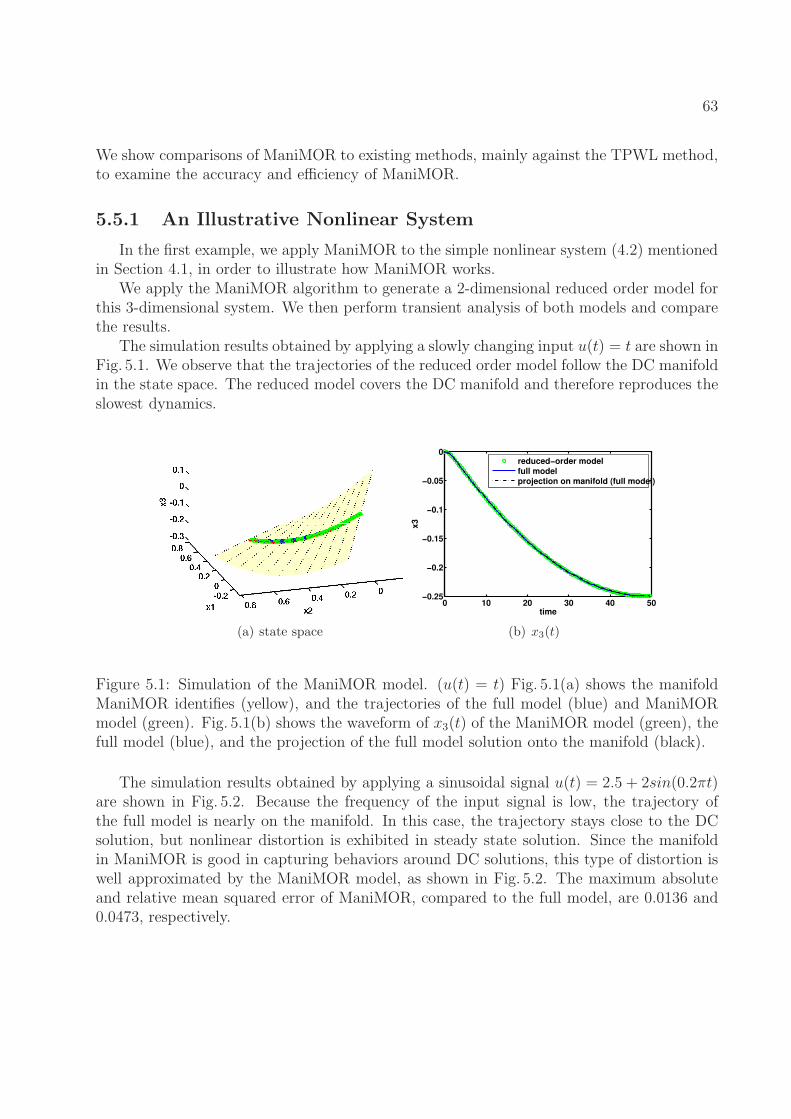
63

We show comparisons of ManiMOR to existing methods, mainly against the TPWL method,to examine the accuracy and efficiency of ManiMOR.

5.5.1 An Illustrative Nonlinear System

In the first example, we apply ManiMOR to the simple nonlinear system (4.2) mentionedin Section 4.1, in order to illustrate how ManiMOR works.

We apply the ManiMOR algorithm to generate a 2-dimensional reduced order model forthis 3-dimensional system. We then perform transient analysis of both models and comparethe results.

The simulation results obtained by applying a slowly changing input u(t) = t are shown inFig. 5.1. We observe that the trajectories of the reduced order model follow the DC manifoldin the state space. The reduced model covers the DC manifold and therefore reproduces theslowest dynamics.

(a) state space

0 10 20 30 40 50−0.25

−0.2

−0.15

−0.1

−0.05

0

time

x3

reduced−order model

full model

projection on manifold (full model)

(b) x3(t)

Figure 5.1: Simulation of the ManiMOR model. (u(t) = t) Fig. 5.1(a) shows the manifoldManiMOR identifies (yellow), and the trajectories of the full model (blue) and ManiMORmodel (green). Fig. 5.1(b) shows the waveform of x3(t) of the ManiMOR model (green), thefull model (blue), and the projection of the full model solution onto the manifold (black).

The simulation results obtained by applying a sinusoidal signal u(t) = 2.5 + 2sin(0.2πt)are shown in Fig. 5.2. Because the frequency of the input signal is low, the trajectory ofthe full model is nearly on the manifold. In this case, the trajectory stays close to the DCsolution, but nonlinear distortion is exhibited in steady state solution. Since the manifoldin ManiMOR is good in capturing behaviors around DC solutions, this type of distortion iswell approximated by the ManiMOR model, as shown in Fig. 5.2. The maximum absoluteand relative mean squared error of ManiMOR, compared to the full model, are 0.0136 and0.0473, respectively.

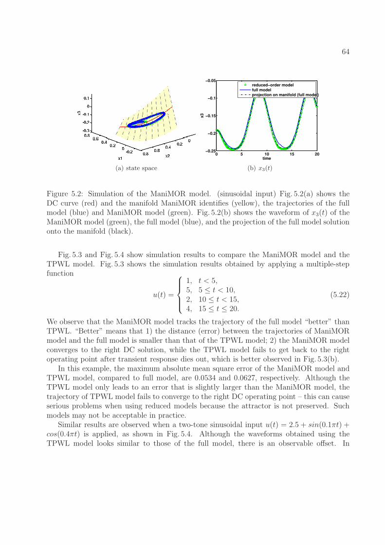
64

(a) state space

0 5 10 15 20−0.25

−0.2

−0.15

−0.1

−0.05

time

x3


full modelprojection on manifold (full model)

(b) x3(t)

Figure 5.2: Simulation of the ManiMOR model. (sinusoidal input) Fig. 5.2(a) shows theDC curve (red) and the manifold ManiMOR identifies (yellow), the trajectories of the fullmodel (blue) and ManiMOR model (green). Fig. 5.2(b) shows the waveform of x3(t) of theManiMOR model (green), the full model (blue), and the projection of the full model solutiononto the manifold (black).

Fig. 5.3 and Fig. 5.4 show simulation results to compare the ManiMOR model and theTPWL model. Fig. 5.3 shows the simulation results obtained by applying a multiple-stepfunction

u(t) =

1, t < 5,5, 5 ≤ t < 10,2, 10 ≤ t < 15,4, 15 ≤ t ≤ 20.

(5.22)

We observe that the ManiMOR model tracks the trajectory of the full model “better” thanTPWL. “Better” means that 1) the distance (error) between the trajectories of ManiMORmodel and the full model is smaller than that of the TPWL model; 2) the ManiMOR modelconverges to the right DC solution, while the TPWL model fails to get back to the rightoperating point after transient response dies out, which is better observed in Fig. 5.3(b).

In this example, the maximum absolute mean square error of the ManiMOR model andTPWL model, compared to full model, are 0.0534 and 0.0627, respectively. Although theTPWL model only leads to an error that is slightly larger than the ManiMOR model, thetrajectory of TPWL model fails to converge to the right DC operating point – this can causeserious problems when using reduced models because the attractor is not preserved. Suchmodels may not be acceptable in practice.

Similar results are observed when a two-tone sinusoidal input u(t) = 2.5 + sin(0.1πt) +cos(0.4πt) is applied, as shown in Fig. 5.4. Although the waveforms obtained using theTPWL model looks similar to those of the full model, there is an observable offset. In

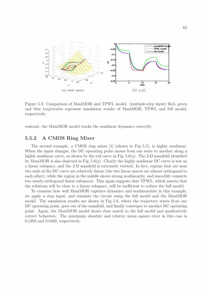
65

(a) state space

0 5 10 15 20−0.35

−0.3

−0.25

−0.2

−0.15

−0.1

−0.05

0

time

x3

maniMOR model

TPWL model

full model

(b) x3(t)

Figure 5.3: Comparison of ManiMOR and TPWL model. (multiple-step input) Red, greenand blue trajectories represent simulation results of ManiMOR, TPWL and full model,respectively.

contrast, the ManiMOR model tracks the nonlinear dynamics correctly.

5.5.2 A CMOS Ring Mixer

The second example, a CMOS ring mixer [1] (shown in Fig. 5.5), is highly nonlinear.When the input changes, the DC operating point moves from one state to another along ahighly nonlinear curve, as shown by the red curve in Fig. 5.6(a). The 2-D manifold identifiedby ManiMOR is also depicted in Fig. 5.6(a). Clearly the highly nonlinear DC curve is not ona linear subspace, and the 2-D manifold is extremely twisted. In fact, regions that are neartwo ends of the DC curve are relatively linear (the two linear spaces are almost orthogonal toeach other), while the region in the middle shows strong nonlinearity, and smoothly connectstwo nearly-orthogonal linear subspaces. This again suggests that TPWL, which asserts thatthe solutions will be close to a linear subspace, will be inefficient to reduce the full model.

To examine how well ManiMOR captures dynamics and nonlinearities in this example,we apply a step input, and simulate the circuit using the full model and the ManiMORmodel. The simulation results are shown in Fig. 5.6, where the trajectory starts from oneDC operating point, goes out of the manifold, and finally converges to another DC operatingpoint. Again, the ManiMOR model shows close match to the full model and qualitativelycorrect behaviors. The maximum absolute and relative mean square error in this case is0.1293 and 0.0492, respectively.

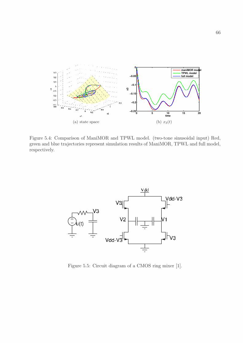
66

(a) state space

0 5 10 15 20−0.25

−0.2

−0.15

−0.1

−0.05

0

time

x3

maniMOR model

TPWL modelfull model

(b) x3(t)

Figure 5.4: Comparison of ManiMOR and TPWL model. (two-tone sinusoidal input) Red,green and blue trajectories represent simulation results of ManiMOR, TPWL and full model,respectively.

Figure 5.5: Circuit diagram of a CMOS ring mixer [1].

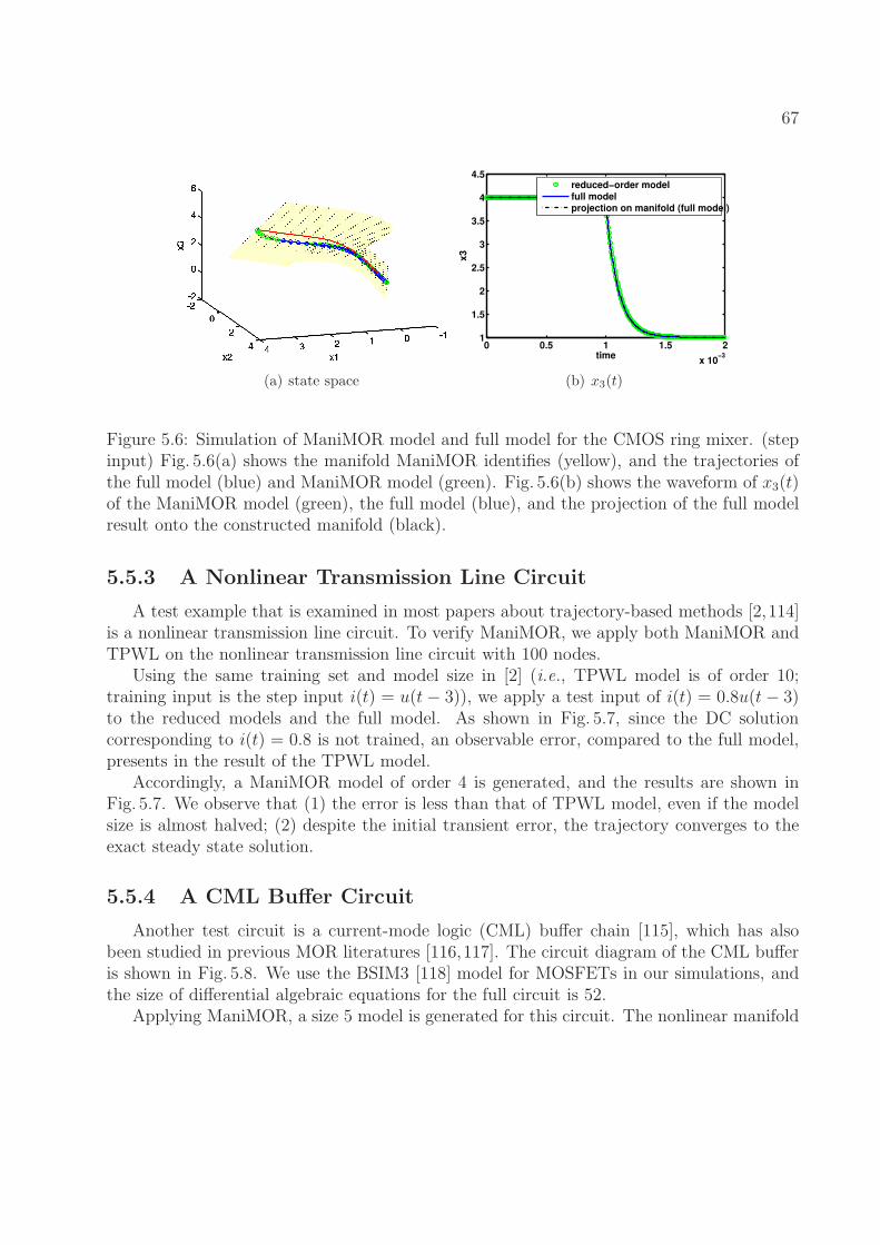
67

(a) state space

0 0.5 1 1.5 2

x 10−3

1

1.5

2

2.5

3

3.5

4

4.5

time

x3


full modelprojection on manifold (full model)

(b) x3(t)

Figure 5.6: Simulation of ManiMOR model and full model for the CMOS ring mixer. (stepinput) Fig. 5.6(a) shows the manifold ManiMOR identifies (yellow), and the trajectories ofthe full model (blue) and ManiMOR model (green). Fig. 5.6(b) shows the waveform of x3(t)of the ManiMOR model (green), the full model (blue), and the projection of the full modelresult onto the constructed manifold (black).

5.5.3 A Nonlinear Transmission Line Circuit

A test example that is examined in most papers about trajectory-based methods [2,114]is a nonlinear transmission line circuit. To verify ManiMOR, we apply both ManiMOR andTPWL on the nonlinear transmission line circuit with 100 nodes.

Using the same training set and model size in [2] (i.e., TPWL model is of order 10;training input is the step input i(t) = u(t− 3)), we apply a test input of i(t) = 0.8u(t− 3)to the reduced models and the full model. As shown in Fig. 5.7, since the DC solutioncorresponding to i(t) = 0.8 is not trained, an observable error, compared to the full model,presents in the result of the TPWL model.

Accordingly, a ManiMOR model of order 4 is generated, and the results are shown inFig. 5.7. We observe that (1) the error is less than that of TPWL model, even if the modelsize is almost halved; (2) despite the initial transient error, the trajectory converges to theexact steady state solution.

5.5.4 A CML Buffer Circuit

Another test circuit is a current-mode logic (CML) buffer chain [115], which has alsobeen studied in previous MOR literatures [116,117]. The circuit diagram of the CML bufferis shown in Fig. 5.8. We use the BSIM3 [118] model for MOSFETs in our simulations, andthe size of differential algebraic equations for the full circuit is 52.

Applying ManiMOR, a size 5 model is generated for this circuit. The nonlinear manifold

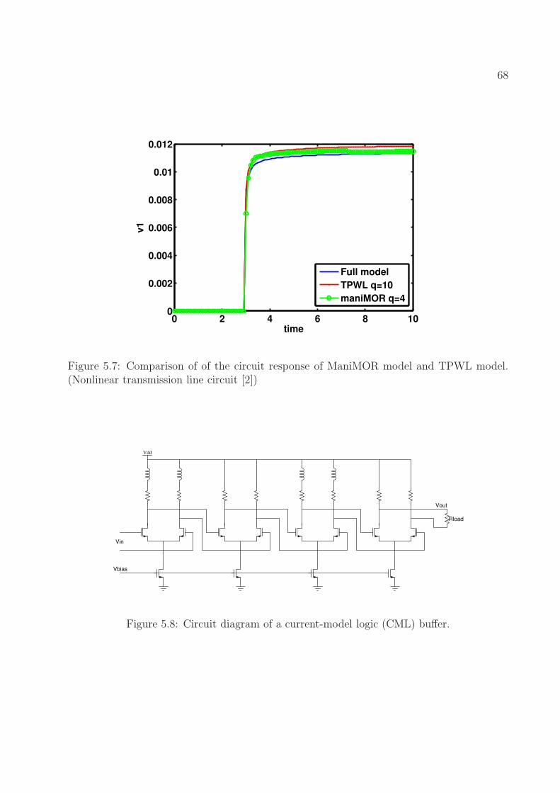
68

0 2 4 6 8 100

0.002

0.004

0.006

0.008

0.01

0.012

time

v1

Full model

TPWL q=10

maniMOR q=4

Figure 5.7: Comparison of of the circuit response of ManiMOR model and TPWL model.(Nonlinear transmission line circuit [2])

Vdd

Vbias

Vin

Vout

Rload

Figure 5.8: Circuit diagram of a current-model logic (CML) buffer.

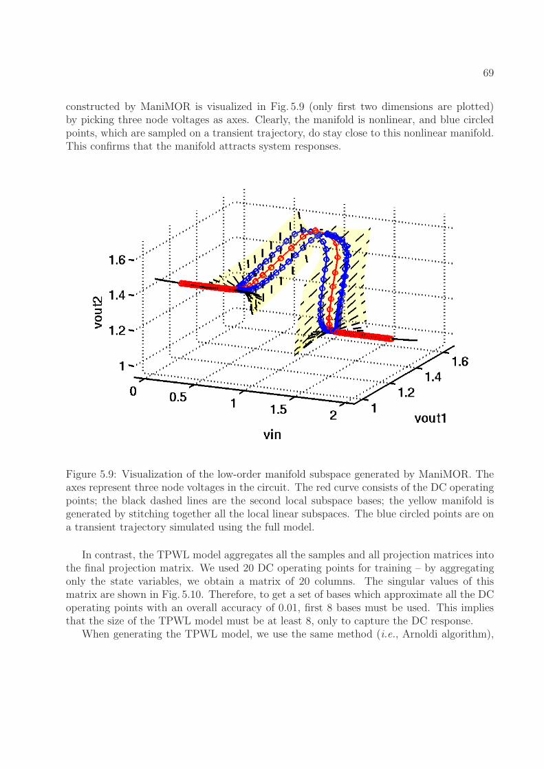
69

constructed by ManiMOR is visualized in Fig. 5.9 (only first two dimensions are plotted)by picking three node voltages as axes. Clearly, the manifold is nonlinear, and blue circledpoints, which are sampled on a transient trajectory, do stay close to this nonlinear manifold.This confirms that the manifold attracts system responses.

Figure 5.9: Visualization of the low-order manifold subspace generated by ManiMOR. Theaxes represent three node voltages in the circuit. The red curve consists of the DC operatingpoints; the black dashed lines are the second local subspace bases; the yellow manifold isgenerated by stitching together all the local linear subspaces. The blue circled points are ona transient trajectory simulated using the full model.

In contrast, the TPWL model aggregates all the samples and all projection matrices intothe final projection matrix. We used 20 DC operating points for training – by aggregatingonly the state variables, we obtain a matrix of 20 columns. The singular values of thismatrix are shown in Fig. 5.10. Therefore, to get a set of bases which approximate all the DCoperating points with an overall accuracy of 0.01, first 8 bases must be used. This impliesthat the size of the TPWL model must be at least 8, only to capture the DC response.

When generating the TPWL model, we use the same method (i.e., Arnoldi algorithm),

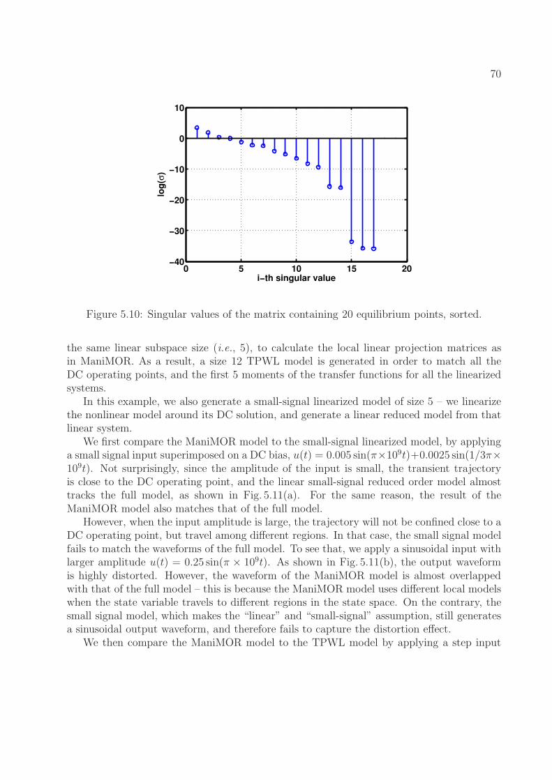
70

0 5 10 15 20−40

−30

−20

−10

0

10

i−th singular value

log

(σ)

Figure 5.10: Singular values of the matrix containing 20 equilibrium points, sorted.

the same linear subspace size (i.e., 5), to calculate the local linear projection matrices asin ManiMOR. As a result, a size 12 TPWL model is generated in order to match all theDC operating points, and the first 5 moments of the transfer functions for all the linearizedsystems.

In this example, we also generate a small-signal linearized model of size 5 – we linearizethe nonlinear model around its DC solution, and generate a linear reduced model from thatlinear system.

We first compare the ManiMOR model to the small-signal linearized model, by applyinga small signal input superimposed on a DC bias, u(t) = 0.005 sin(π×109t)+0.0025 sin(1/3π×109t). Not surprisingly, since the amplitude of the input is small, the transient trajectoryis close to the DC operating point, and the linear small-signal reduced order model almosttracks the full model, as shown in Fig. 5.11(a). For the same reason, the result of theManiMOR model also matches that of the full model.

However, when the input amplitude is large, the trajectory will not be confined close to aDC operating point, but travel among different regions. In that case, the small signal modelfails to match the waveforms of the full model. To see that, we apply a sinusoidal input withlarger amplitude u(t) = 0.25 sin(π × 109t). As shown in Fig. 5.11(b), the output waveformis highly distorted. However, the waveform of the ManiMOR model is almost overlappedwith that of the full model – this is because the ManiMOR model uses different local modelswhen the state variable travels to different regions in the state space. On the contrary, thesmall signal model, which makes the “linear” and “small-signal” assumption, still generatesa sinusoidal output waveform, and therefore fails to capture the distortion effect.

We then compare the ManiMOR model to the TPWL model by applying a step input

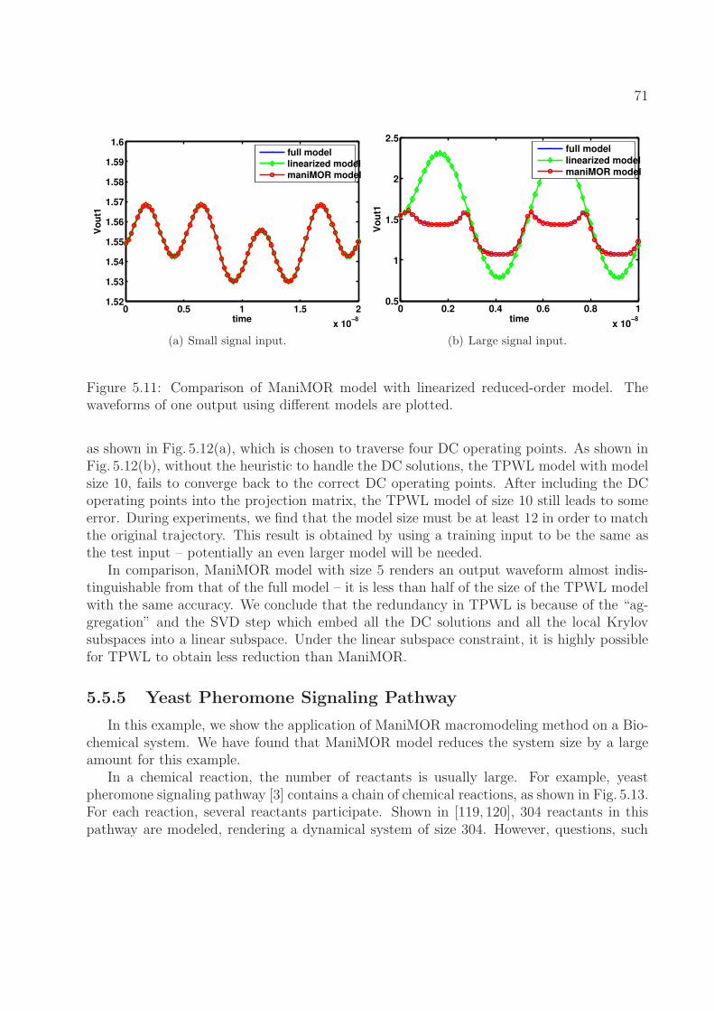
71

0 0.5 1 1.5 2

x 10−8

1.52

1.53

1.54

1.55

1.56

1.57

1.58

1.59

1.6

time

Vo

ut1

full model

linearized model

maniMOR model

(a) Small signal input.

0 0.2 0.4 0.6 0.8 1

x 10−8

0.5

1

1.5

2

2.5

time

Vo

ut1

full model

linearized model

maniMOR model

(b) Large signal input.

Figure 5.11: Comparison of ManiMOR model with linearized reduced-order model. Thewaveforms of one output using different models are plotted.

as shown in Fig. 5.12(a), which is chosen to traverse four DC operating points. As shown inFig. 5.12(b), without the heuristic to handle the DC solutions, the TPWL model with modelsize 10, fails to converge back to the correct DC operating points. After including the DCoperating points into the projection matrix, the TPWL model of size 10 still leads to someerror. During experiments, we find that the model size must be at least 12 in order to matchthe original trajectory. This result is obtained by using a training input to be the same asthe test input – potentially an even larger model will be needed.

In comparison, ManiMOR model with size 5 renders an output waveform almost indis-tinguishable from that of the full model – it is less than half of the size of the TPWL modelwith the same accuracy. We conclude that the redundancy in TPWL is because of the “ag-gregation” and the SVD step which embed all the DC solutions and all the local Krylovsubspaces into a linear subspace. Under the linear subspace constraint, it is highly possiblefor TPWL to obtain less reduction than ManiMOR.

5.5.5 Yeast Pheromone Signaling Pathway

In this example, we show the application of ManiMOR macromodeling method on a Bio-chemical system. We have found that ManiMOR model reduces the system size by a largeamount for this example.

In a chemical reaction, the number of reactants is usually large. For example, yeastpheromone signaling pathway [3] contains a chain of chemical reactions, as shown in Fig. 5.13.For each reaction, several reactants participate. Shown in [119, 120], 304 reactants in thispathway are modeled, rendering a dynamical system of size 304. However, questions, such

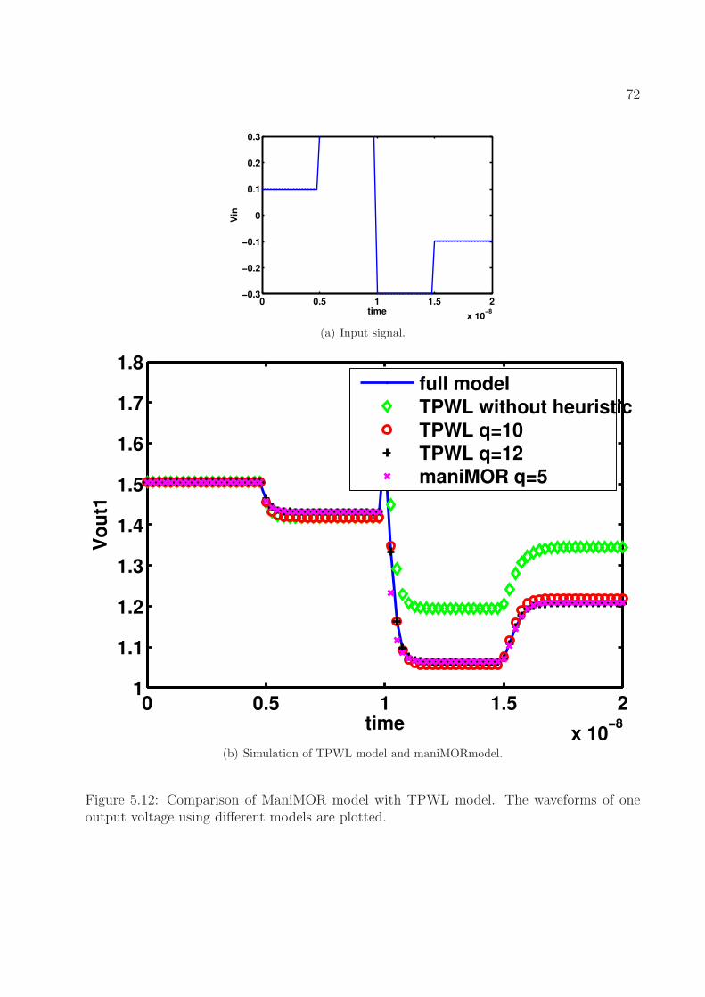
72

0 0.5 1 1.5 2

x 10−8

−0.3

−0.2

−0.1

0

0.1

0.2

0.3

time

Vin

(a) Input signal.

0 0.5 1 1.5 2

x 10−8

1

1.1

1.2

1.3

1.4

1.5

1.6

1.7

1.8

time

Vo

ut1

full model

TPWL without heuristic

TPWL q=10

TPWL q=12

maniMOR q=5

(b) Simulation of TPWL model and maniMORmodel.

Figure 5.12: Comparison of ManiMOR model with TPWL model. The waveforms of oneoutput voltage using different models are plotted.

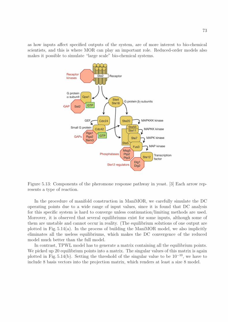
73

as how inputs affect specified outputs of the system, are of more interest to bio-chemicalscientists, and this is where MOR can play an important role. Reduced-order models alsomakes it possible to simulate “large scale” bio-chemical systems.

Figure 5.13: Components of the pheromone response pathway in yeast. [3] Each arrow rep-resents a type of reaction.

In the procedure of manifold construction in ManiMOR, we carefully simulate the DCoperating points due to a wide range of input values, since it is found that DC analysisfor this specific system is hard to converge unless continuation/limiting methods are used.Moreover, it is observed that several equilibriums exist for some inputs, although some ofthem are unstable and cannot occur in reality. (The equilibrium solutions of one output areplotted in Fig. 5.14(a). In the process of building the ManiMOR model, we also implicitlyeliminates all the useless equilibriums, which makes the DC convergence of the reducedmodel much better than the full model.

In contrast, TPWL model has to generate a matrix containing all the equilibrium points.We picked up 20 equilibrium points into a matrix. The singular values of this matrix is againplotted in Fig. 5.14(b). Setting the threshold of the singular value to be 10−10, we have toinclude 8 basis vectors into the projection matrix, which renders at least a size 8 model.

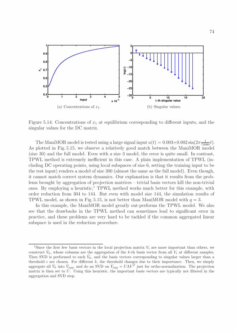
74

0 1 2 3 4 5

x 10−3

0.4

0.5

0.6

0.7

0.8

0.9

1

input

x1

(a) Concentrations of x1.

0 5 10 15 20−30

−25

−20

−15

−10

−5

0

5

i−th singular value

log

(σ)

(b) Singular values.

Figure 5.14: Concentrations of x1 at equilibrium corresponding to different inputs, and thesingular values for the DC matrix.

The ManiMORmodel is tested using a large signal input u(t) = 0.003+0.002 sin(2π 172000

t).As plotted in Fig. 5.15, we observe a relatively good match between the ManiMOR model(size 30) and the full model. Even with a size 3 model, the error is quite small. In contrast,TPWL method is extremely inefficient in this case. A plain implementation of TPWL (in-cluding DC operating points, using local subspaces of size 6, setting the training input to bethe test input) renders a model of size 300 (almost the same as the full model). Even though,it cannot match correct system dynamics. Our explanation is that it results from the prob-lems brought by aggregation of projection matrices – trivial basis vectors kill the non-trivialones. By employing a heuristic,1 TPWL method works much better for this example, withorder reduction from 304 to 144. But even with model size 144, the simulation results ofTPWL model, as shown in Fig. 5.15, is not better than ManiMOR model with q = 3.

In this example, the ManiMOR model greatly out-performs the TPWL model. We alsosee that the drawbacks in the TPWL method can sometimes lead to significant error inpractice, and these problems are very hard to be tackled if the common aggregated linearsubspace is used in the reduction procedure.

1Since the first few basis vectors in the local projection matrix Vi are more important than others, weconstruct Vk, whose columns are the aggregation of the k-th basis vector from all Vi at different samples.Then SVD is performed to each Vk, and the basis vectors corresponding to singular values larger than athreshold ǫ are chosen. For different k, the threshold changes due to their importance. Then, we simplyaggregate all Vk into Vagg, and do an SVD on Vagg = UΛV T just for ortho-normalization. The projectionmatrix is then set to U . Using this heuristic, the important basis vectors are typically not filtered in theaggregation and SVD step.

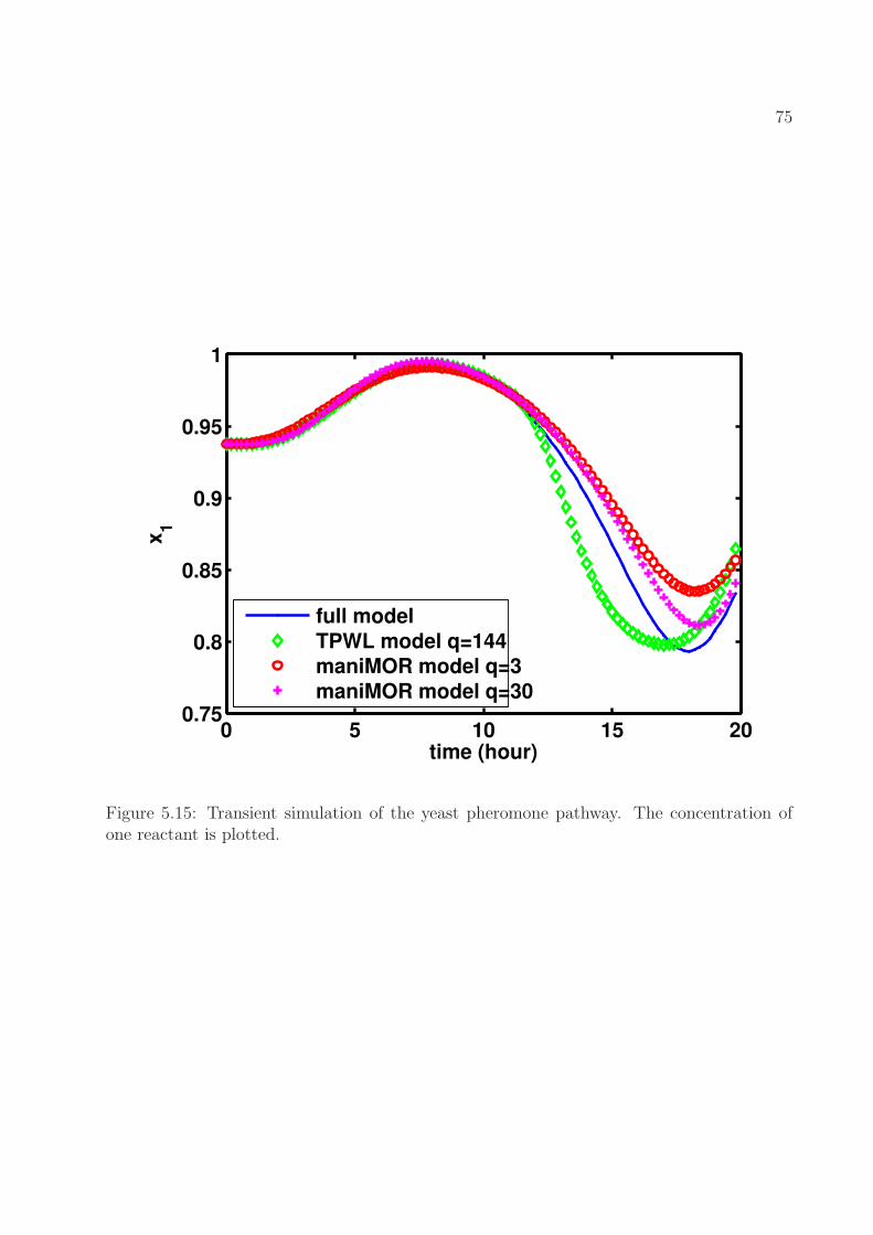
75

0 5 10 15 200.75

0.8

0.85

0.9

0.95

1

time (hour)

x1

full model

TPWL model q=144

maniMOR model q=3

maniMOR model q=30

Figure 5.15: Transient simulation of the yeast pheromone pathway. The concentration ofone reactant is plotted.

76

Chapter 6

QLMOR: MOR using EquivalentQuadratic-Linear Systems

In this chapter, we present another nonlinear projection-based MOR technique, based onan “equivalent” quadratic-linear system representation of the original nonlinear system. Thisrepresentation is exact in the sense that the solution of the equivalent system is exactly thesame as the original nonlinear system. Therefore, the quadratic-linear model differentiatesitself from Taylor-expansion-based quadratic/polynomial models. The reduction is thenperformed on the quadratic-linear representation to obtain a quadratic-linear reduced model.

We first summarize previous work on polynomial reduced order modeling techniques, andthe major problems therein. We then present algorithms that transform almost all nonlineardifferential equations to their quadratic-linear representation. With the resulting quadratic-linear representation, we perform Volterra analysis, and derive a reduced-order modelingtechnique. We show experimental results and comparisons to other techniques.

6.1 Volterra-Series Based Reduction of Polynomial Sys-

tems

Previous Volterra-series based MOR methods [106, 107, 121] are derived from the resultthat the response of a nonlinear system can be decomposed into responses of a series of ho-mogeneous nonlinear systems, i.e., the system response x(t) can be written as the summationof responses of all n-th order homogeneous nonlinear systems xn(t):

x(t) =

∞∑

n=1

xn(t), (6.1)

77

where

xn(t) =

∫ ∞

−∞

· · ·∫ ∞

−∞

hn(σ1, · · · , σn)

u(t− σ1) · · ·u(t− σn) dσ1 · · · dσn.

(6.2)

In (6.2), hn(σ1, · · · , σn) is the Volterra kernel of order n, and we can define Hn(s1, · · · , sn),the transfer function of order n, to be

Hn(s1, · · · , sn) =∫ ∞

−∞

· · ·∫ ∞

−∞

hn(σ1, · · · , σn)

e−(s1σ1+···+snσn) dσ1 · · · dσn,

(6.3)

which is the multi-variable Laplace transform of hn(σ1, · · · , σn) [105].Previous Volterra-series based methods can be summarized in four steps:

1. Perform a Taylor expansion of the nonlinear function f(x), i.e., expand f(x) in aseries of multidimensional polynomials, and truncate the expansion to a predefinedorder (e.g., 3, as shown in (6.4)1).

Cd

dtx = G1x+G2x⊗ x+G3x⊗ x⊗ x+Bu, (6.4)

where C, G1, G2, G3 and B are of appropriate dimensions given x ∈ RN and u ∈ R.

2. For methods based on bilinear forms, perform a Carleman bilinearization [73] on (6.4)to obtain a bilinear approximation

Cd

dtx = Gx+Dxu+Bu, (6.5)

where C, G, D and B are of appropriate dimensions.

3. Construct a projection matrix V ∈ RN×Nr to match the moments of Hn, n = 1, 2, 3, · · ·

up to a given order. E.g., to match up to the second order moments of H2(s1, s2)means to match the coefficients of terms 1, s1, s2, s

21, s1s2, s

22 in the Taylor expansion of

H2(s1, s2) [106].

4. Construct the projected reduced system. E.g.,

Crd

dtxr = Gr,1xr +Gr,2xr ⊗ xr +Gr,3xr ⊗ xr ⊗ xr +Bru (6.6)

1For notational simplicity, we will sometimes use x 2© to denote ~x⊗ ~x, x 3© to denote ~x⊗ ~x⊗ ~x, etc..

78

by defining

x = V xr,

Cr = V TCV,

Br = V TB,

Gr,1 = V TG1V,

Gr,2 = V TG2(V ⊗ V ),

Gr,3 = V TG3(V ⊗ V ⊗ V ).

(6.7)

The common step in [106,107,121] is Taylor approximation. This results in three majordrawbacks that limit the wide applicability of these methods. Firstly, the convergence ofthe Volterra system representation is only valid when |u| ≤ ǫ, for some small ǫ > 0, i.e., for“small” inputs, or the “weakly nonlinear” case. This constraint stems partly from the factthat the Taylor series only converges in a small region around the expansion point. Incorrectbehavior of the reduced model due to large inputs was reported in [107], and similar resultsare reproduced in Section 6.5.2.

Secondly, Taylor expansion typically destroys important global properties of the system,such as passivity and stability. For example [107], the quadratic approximation for ex, whichis part of the I-V curve of a diode, around x = 0 leads to an artificial diode that cangenerate energy when the voltage applied is negative. As a result, the reduced model, whichis created using the Taylor approximated system as a starting point, will typically not bepassive/stable.

Thirdly, the computational cost for higher-order terms such as Gr,3 xr⊗xr⊗xr dominatesthe computational cost of the reduced model. Since xr ∈ R

Nr , Gr,3 ∈ RNr×N3

r , and withGr,3 usually dense, the computational cost is O(N4

r ). (It is possible to make Gr,3 of asmaller size by combining terms in xr ⊗ xr ⊗ xr, but the computational complexity does notchange.) Although it is N -independent, it can potentially be too expensive to use in practice.Moreover, it is generally difficult to accurately extract the high-order matrices G2, G3, · · · ,which also constrains applications of Taylor-expansion based methods.

Remark MOR methods based on bilinear forms and Volterra series [107] actually definea nonlinear projection – e.g., by explicitly writing out the differential equations for ~x ⊗~x, ~x ⊗ ~x ⊗ ~x, the final projection is defined by xr = V T [xT , xT ⊗ xT , xT ⊗ xT ⊗ xT ]T , whichis a polynomial projection function. In this sense, QLMOR indeed allows a richer set ofprojections than those in previous methods [107].

Briefly summarizing this section, we list in Table 6.1 the main drawbacks and difficultiesthat have not been solved in existing MOR methods, and how well QLMOR addresses thesedrawbacks.

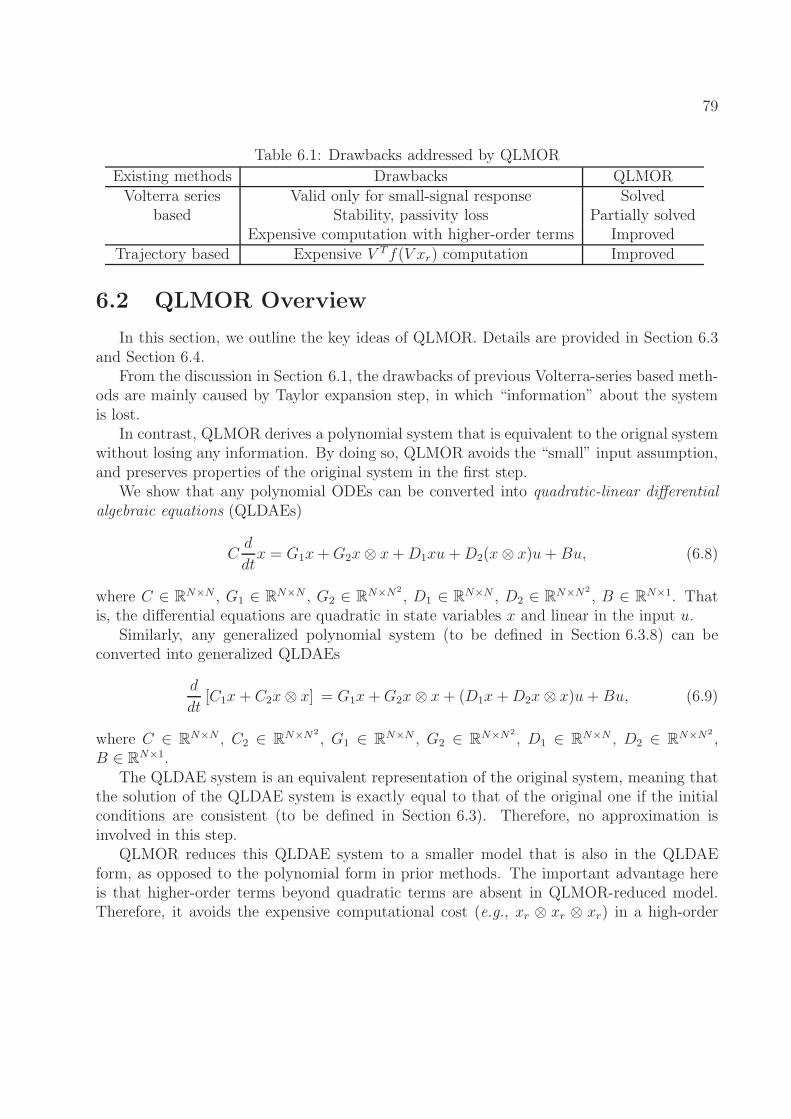
79

Table 6.1: Drawbacks addressed by QLMOR

Existing methods Drawbacks QLMORVolterra series Valid only for small-signal response Solved

based Stability, passivity loss Partially solvedExpensive computation with higher-order terms Improved

Trajectory based Expensive V Tf(V xr) computation Improved

6.2 QLMOR Overview

In this section, we outline the key ideas of QLMOR. Details are provided in Section 6.3and Section 6.4.

From the discussion in Section 6.1, the drawbacks of previous Volterra-series based meth-ods are mainly caused by Taylor expansion step, in which “information” about the systemis lost.

In contrast, QLMOR derives a polynomial system that is equivalent to the orignal systemwithout losing any information. By doing so, QLMOR avoids the “small” input assumption,and preserves properties of the original system in the first step.

We show that any polynomial ODEs can be converted into quadratic-linear differentialalgebraic equations (QLDAEs)

Cd

dtx = G1x+G2x⊗ x+D1xu+D2(x⊗ x)u+Bu, (6.8)

where C ∈ RN×N , G1 ∈ R

N×N , G2 ∈ RN×N2

, D1 ∈ RN×N , D2 ∈ R

N×N2

, B ∈ RN×1. That

is, the differential equations are quadratic in state variables x and linear in the input u.Similarly, any generalized polynomial system (to be defined in Section 6.3.8) can be

converted into generalized QLDAEs

d

dt[C1x+ C2x⊗ x] = G1x+G2x⊗ x+ (D1x+D2x⊗ x)u+Bu, (6.9)

where C ∈ RN×N , C2 ∈ R

N×N2

, G1 ∈ RN×N , G2 ∈ R

N×N2

, D1 ∈ RN×N , D2 ∈ R

N×N2

,B ∈ R

N×1.The QLDAE system is an equivalent representation of the original system, meaning that

the solution of the QLDAE system is exactly equal to that of the original one if the initialconditions are consistent (to be defined in Section 6.3). Therefore, no approximation isinvolved in this step.

QLMOR reduces this QLDAE system to a smaller model that is also in the QLDAEform, as opposed to the polynomial form in prior methods. The important advantage hereis that higher-order terms beyond quadratic terms are absent in QLMOR-reduced model.Therefore, it avoids the expensive computational cost (e.g., xr ⊗ xr ⊗ xr) in a high-order

80

polynomial reduced model, and quadratic terms dominates the computational complexity.The reduced order model is obtained by projection of the QLDAE system. While it looks

like a linear projection (of the QLDAE system), it indeed defines a nonlinear projection (ofthe original system). To obtain the minimum subspace in the sense of moment matching,we analyze the transfer functions of systems in the QLDAE form, and results related toprior methods are derived. For example, it turns out that the moments of H2(s1, s2) of aQLDAE system are a summation of the moments of H2(s1, s2) of a quadratic system anda bilinear system – direct application of existing codes are possible. In our algorithm, wealso avoid explicit moment evaluations, and therefore the algorithm has better numericalstability properties.

Another point to note is that QLMOR serves as a new core method that can be combinedwith any trajectory-based methods. For example, in TPWL method, to generate reducedmodels along a trajectory, previous Krylov-subspace methods or TBR methods can be re-placed with QLMOR straightforwardly, potentially leading to a more accurate model andless number of regions along the trajectory. For another example, POD method can be di-rectly applied to the transformed QLDAE system, which results in a reduced model whosecomputational cost is lower than the usual POD reduced model if the reduced model sizeremains the same.

To summarize, QLMOR is composed of three steps:

1. construct an equivalent polynomial system from the orignal system;

2. construct an equivalent quadratic-linear system from the polynomial system;

3. reduced the quadratic-linear system to a smaller quadratic-linear system.

We chart in Fig. 6.1 the basic flow of QLMOR, as well as the flow of MOR based on poly-nomial systems and bilinear systems for comparison. In what follows, Section 6.3 presentsthe polynomialization and the quadratic-linearization procedure, and Section 6.4 discussesthe reduction step.

6.3 Quadratic-Linearization Procedure

In this section, we develop an algorithm to convert systems of ordinary differential equa-tions to an equivalent system which has functions that are quadratic in state variables andlinear in inputs. We call it quadratic-linearization procedure, and we call the resultingsystem QLDAEs (quadratic-linear differential-algebraic equations). We also discuss exten-sions to quadratic-linearize DAEs in the end of this section.

Considering nonlinear ODEs, the quadratic-linearization procedure is composed of twosteps:

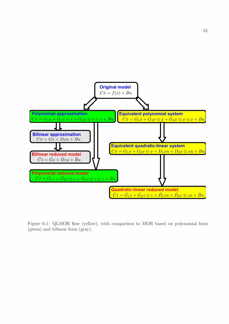
81

Figure 6.1: QLMOR flow (yellow), with comparison to MOR based on polynomial form(green) and bilinear form (gray).

82

1. convert the original nonlinear ODEs

d

dtx = f(x) +Bu (6.10)

into a polynomial system;

2. convert the polynomial system into QLDAEs.

We call the first procedure polynomialization, the second procedure quadratic-linearizationof a polynomial system.

6.3.1 Nonlinear ODEs and Polynomial Systems

To be more specific, we consider “semi-general” nonlinear ODEs (6.10) where the non-linear functions f(x) = [f1(x), · · · , fN(x)] can be written as a linear combination of a set ofelementary functions gi(x), i = 1, · · · , k, i.e., the differential equation for xi is

d

dtxi = pTi x+ ai,1g1(x) + ai,2g2(x) + · · ·+ ai,kgk(x) + biu, ∀i = 1, · · · , N, (6.11)

where pi ∈ RN×1, ai,j ∈ R, bi ∈ R. In matrix form, (6.11) can be written as

d

dtx = Px+ Ag(x) +Bu, (6.12)

where P T = [p1, · · · , pN ], A = [ai,j], g(x) = [g1(x); · · · , gk(x)] and B = [b1; · · · ; bN ]. Notethat A is extremely sparse due to the fact that each differential equation typically containsjust a few nonlinear functions.

As mentioned in Section 2.7, this form of differential equations is prevalent in circuitsimulation, as well as other engineering problems. For example, in circuit MNA equa-tions [108, 109], each gi(x) represents the current flowing into a node from a specific device;in chemical rate equations, each gi(x) represents the reaction rate according to a specificreaction; in mechanical applications, gi(x) is the force to the system.

The elementary functions gi(x) include, but not limited to, the ones listed in Table 6.2,and compositions of these elementary functions. Because of the function composition, thenonlinear functions in Table 6.2 in fact cover a very rich set of nonlinear functions that arealmost adequate in engineering problems.

Specifically, in circuit simulation, two important classes of models use functions that area subset of composition of these elementary functions.

The first class is the most commonly used transistor models, such as BSIM [118] or PSPmodels [123]. These models are written in C/C++, and contain “if-else” statements toimplement piecewise-linear functions. For example, the C code

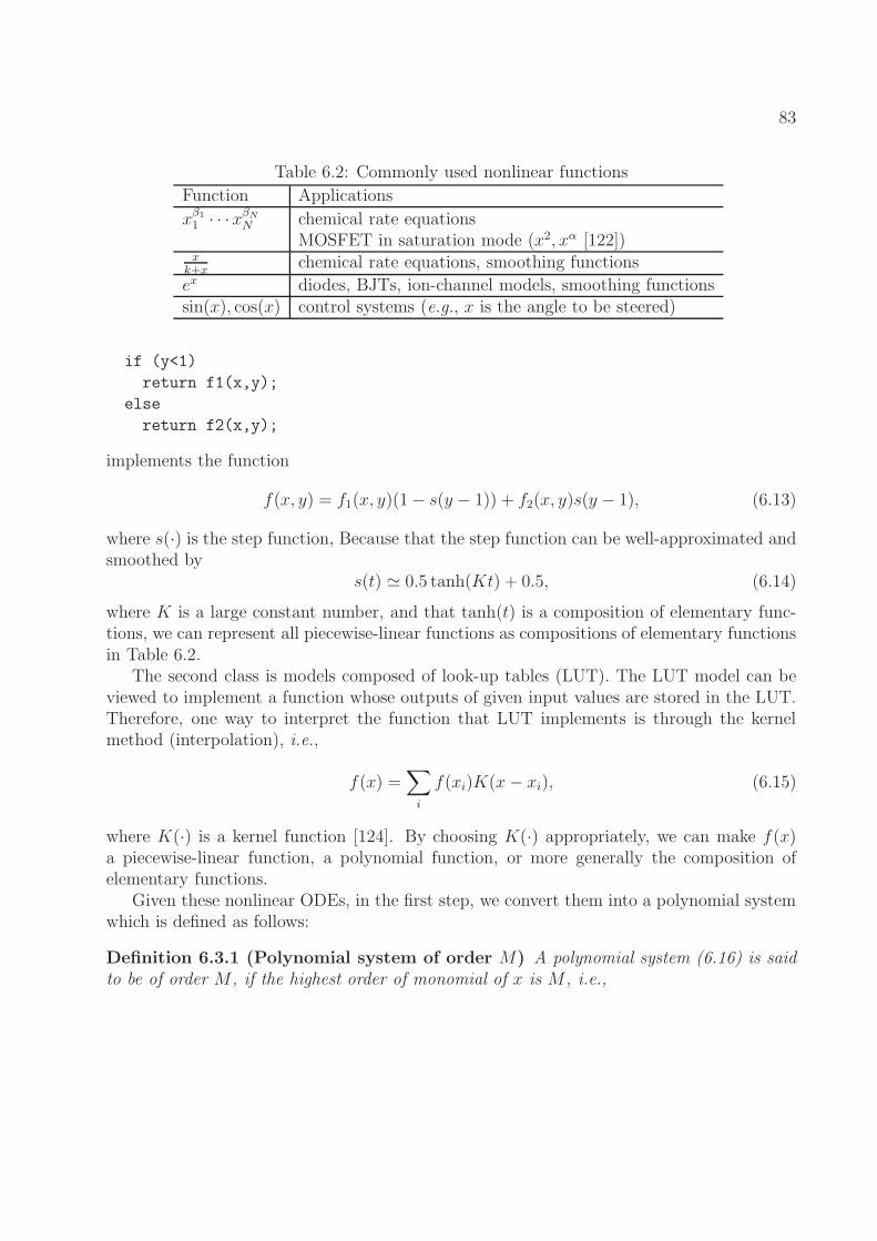
83

Table 6.2: Commonly used nonlinear functions

Function Applications

xβ1

1 · · ·xβN

N chemical rate equationsMOSFET in saturation mode (x2, xα [122])

xk+x

chemical rate equations, smoothing functions

ex diodes, BJTs, ion-channel models, smoothing functionssin(x), cos(x) control systems (e.g., x is the angle to be steered)

if (y<1)

return f1(x,y);

else

return f2(x,y);

implements the function

f(x, y) = f1(x, y)(1− s(y − 1)) + f2(x, y)s(y − 1), (6.13)

where s(·) is the step function, Because that the step function can be well-approximated andsmoothed by

s(t) ≃ 0.5 tanh(Kt) + 0.5, (6.14)

where K is a large constant number, and that tanh(t) is a composition of elementary func-tions, we can represent all piecewise-linear functions as compositions of elementary functionsin Table 6.2.

The second class is models composed of look-up tables (LUT). The LUT model can beviewed to implement a function whose outputs of given input values are stored in the LUT.Therefore, one way to interpret the function that LUT implements is through the kernelmethod (interpolation), i.e.,

f(x) =∑

i

f(xi)K(x− xi), (6.15)

where K(·) is a kernel function [124]. By choosing K(·) appropriately, we can make f(x)a piecewise-linear function, a polynomial function, or more generally the composition ofelementary functions.

Given these nonlinear ODEs, in the first step, we convert them into a polynomial systemwhich is defined as follows:

Definition 6.3.1 (Polynomial system of order M) A polynomial system (6.16) is saidto be of order M , if the highest order of monomial of x is M , i.e.,

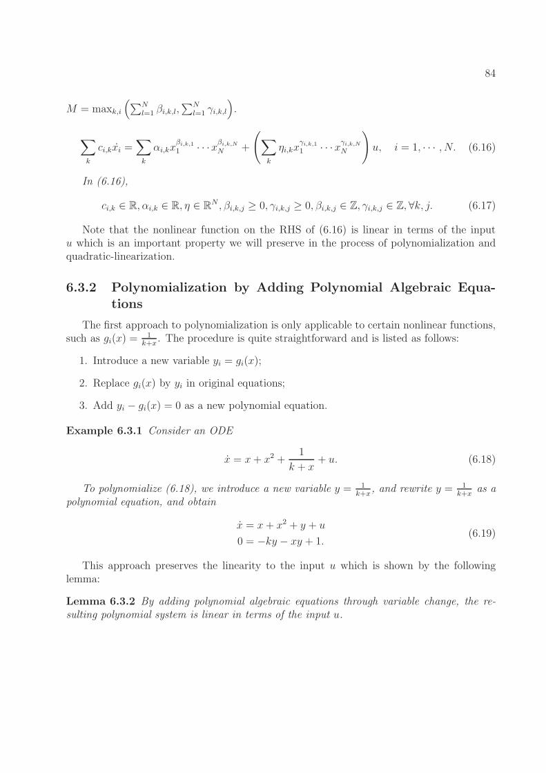
84

M = maxk,i

(

∑Nl=1 βi,k,l,

∑Nl=1 γi,k,l

)

.

∑

k

ci,kxi =∑

k

αi,kxβi,k,1

1 · · ·xβi,k,N

N +

(

∑

k

ηi,kxγi,k,11 · · ·xγi,k,N

N

)

u, i = 1, · · · , N. (6.16)

In (6.16),

ci,k ∈ R, αi,k ∈ R, η ∈ RN , βi,k,j ≥ 0, γi,k,j ≥ 0, βi,k,j ∈ Z, γi,k,j ∈ Z, ∀k, j. (6.17)

Note that the nonlinear function on the RHS of (6.16) is linear in terms of the inputu which is an important property we will preserve in the process of polynomialization andquadratic-linearization.

6.3.2 Polynomialization by Adding Polynomial Algebraic Equa-tions

The first approach to polynomialization is only applicable to certain nonlinear functions,such as gi(x) =

1k+x

. The procedure is quite straightforward and is listed as follows:

1. Introduce a new variable yi = gi(x);

2. Replace gi(x) by yi in original equations;

3. Add yi − gi(x) = 0 as a new polynomial equation.

Example 6.3.1 Consider an ODE

x = x+ x2 +1

k + x+ u. (6.18)

To polynomialize (6.18), we introduce a new variable y = 1k+x

, and rewrite y = 1k+x

as apolynomial equation, and obtain

x = x+ x2 + y + u

0 = −ky − xy + 1.(6.19)

This approach preserves the linearity to the input u which is shown by the followinglemma:

Lemma 6.3.2 By adding polynomial algebraic equations through variable change, the re-sulting polynomial system is linear in terms of the input u.

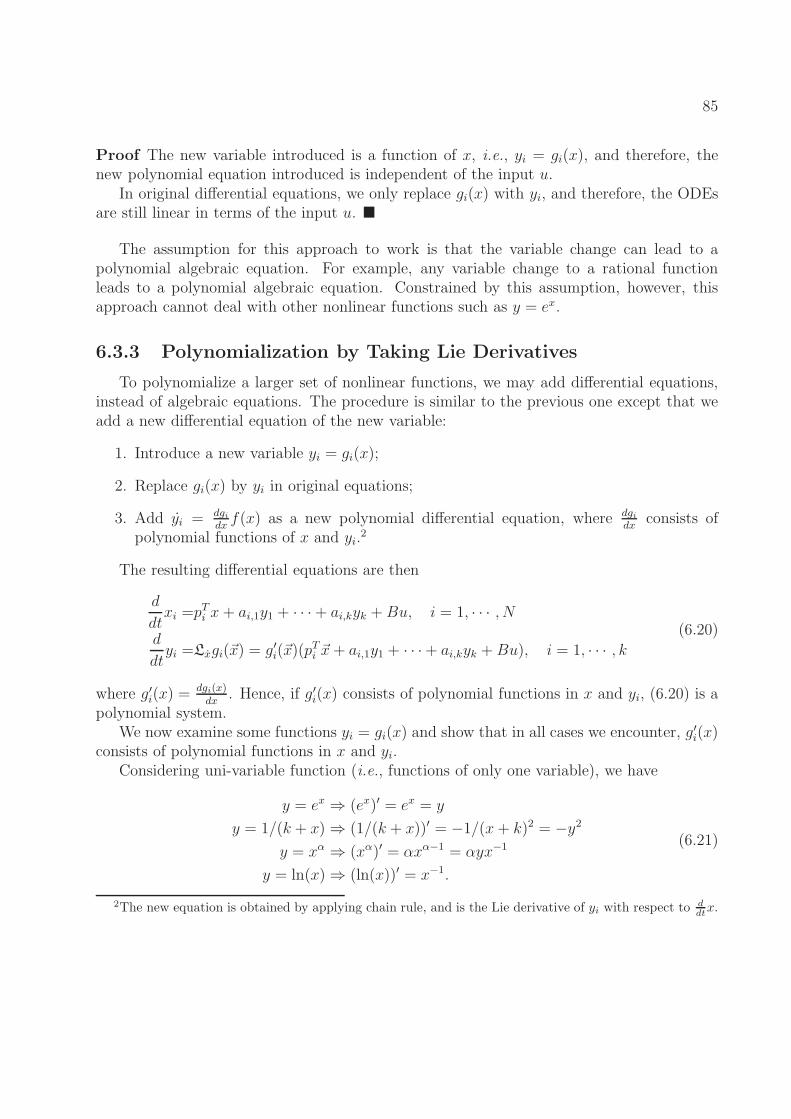
85

Proof The new variable introduced is a function of x, i.e., yi = gi(x), and therefore, thenew polynomial equation introduced is independent of the input u.

In original differential equations, we only replace gi(x) with yi, and therefore, the ODEsare still linear in terms of the input u.

The assumption for this approach to work is that the variable change can lead to apolynomial algebraic equation. For example, any variable change to a rational functionleads to a polynomial algebraic equation. Constrained by this assumption, however, thisapproach cannot deal with other nonlinear functions such as y = ex.

6.3.3 Polynomialization by Taking Lie Derivatives

To polynomialize a larger set of nonlinear functions, we may add differential equations,instead of algebraic equations. The procedure is similar to the previous one except that weadd a new differential equation of the new variable:

1. Introduce a new variable yi = gi(x);

2. Replace gi(x) by yi in original equations;

3. Add yi = dgidxf(x) as a new polynomial differential equation, where dgi

dxconsists of

polynomial functions of x and yi.2

The resulting differential equations are then

d

dtxi =pTi x+ ai,1y1 + · · ·+ ai,kyk +Bu, i = 1, · · · , N

d

dtyi =Lxgi(~x) = g′i(~x)(p

Ti ~x+ ai,1y1 + · · ·+ ai,kyk +Bu), i = 1, · · · , k

(6.20)

where g′i(x) =dgi(x)dx

. Hence, if g′i(x) consists of polynomial functions in x and yi, (6.20) is apolynomial system.

We now examine some functions yi = gi(x) and show that in all cases we encounter, g′i(x)consists of polynomial functions in x and yi.

Considering uni-variable function (i.e., functions of only one variable), we have

y = ex ⇒ (ex)′ = ex = y

y = 1/(k + x)⇒ (1/(k + x))′ = −1/(x+ k)2 = −y2

y = xα ⇒ (xα)′ = αxα−1 = αyx−1

y = ln(x)⇒ (ln(x))′ = x−1.

(6.21)

2The new equation is obtained by applying chain rule, and is the Lie derivative of yi with respect to ddtx.

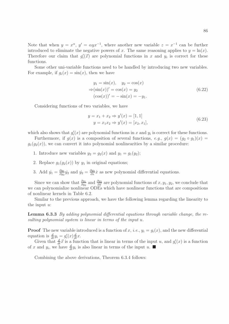
86

Note that when y = xα, y′ = αyx−1, where another new variable z = x−1 can be furtherintroduced to eliminate the negative powers of x. The same reasoning applies to y = ln(x).Therefore our claim that g′i(~x) are polynomial functions in x and yi is correct for thesefunctions.

Some other uni-variable functions need to be handled by introducing two new variables.For example, if gi(x) = sin(x), then we have

y1 = sin(x), y2 = cos(x)

⇒(sin(x))′ = cos(x) = y2

(cos(x))′ = − sin(x) = −y1.(6.22)

Considering functions of two variables, we have

y = x1 + x2 ⇒ y′(x) = [1, 1]

y = x1x2 ⇒ y′(x) = [x2, x1],(6.23)

which also shows that g′i(x) are polynomial functions in x and yi is correct for these functions.Furthermore, if g(x) is a composition of several functions, e.g., g(x) = (g2 g1)(x) =

g1(g2(x)), we can convert it into polynomial nonlinearities by a similar procedure:

1. Introduce new variables y2 = g2(x) and y1 = g1(y2);

2. Replace g1(g2(x)) by y1 in original equations;

3. Add y1 =∂y1∂y2

y2 and y2 =∂y2∂x

x as new polynomial differential equations.

Since we can show that ∂y1∂y2

and ∂y2∂~x

are polynomial functions of x, y1, y2, we conclude thatwe can polynomialize nonlinear ODEs which have nonlinear functions that are compositionsof nonlinear kernels in Table 6.2.

Similar to the previous approach, we have the following lemma regarding the linearity tothe input u:

Lemma 6.3.3 By adding polynomial differential equations through variable change, the re-sulting polynomial system is linear in terms of the input u.

Proof The new variable introduced is a function of x, i.e., yi = gi(x), and the new differentialequation is d

dtyi = g′i(x)

ddtx.

Given that ddt~x is a function that is linear in terms of the input u, and g′i(x) is a function

of x and yi, we have ddtyi is also linear in terms of the input u.

Combining the above derivations, Theorem 6.3.4 follows:

87

Theorem 6.3.4 By iteratively applying polynomialization by adding polynomial algebraicequations and taking Lie derivatives, a nonlinear system with nonlinear functions being com-positions of functions in Table 6.2 can be polynomialized into a polynomial system in theform of (6.16).

Moreover, the size of the equivalent polynomial system is linear with respect to the numberof elementary functions in original ODEs/DAEs.

Proof The proof for the first part is constructive – the procedure described in previoussubsections (also summarized in Algorithm 6 in Section 6.3.4) converts ODEs/DAEs to anequivalent polynomial system.

Regarding the size of the equivalent polynomial system, we note that for an elementaryfunction, we can always polynomialize it by adding constant number (O(1)) of new variablesand equations (normally 1 or 2); For a nonlinear function that is a composition of m elemen-tary functions, i.e., g(x) = g1(g2(· · · gm(x) · · · )), we can always polynomialize it by addingO(m) new variables and equations. Therefore, the size of the equivalent polynomial systemis linear with respect to the number of elementary functions in original ODEs/DAEs.

Remark In circuit applications, the number of elementary functions is linear with respectto the number of nonlinear devices in the circuit. Therefore, the polynomialization procedurescales well with the size of the circuit. Similar results can be obtained for other engineeringproblems.

6.3.4 Polynomialization Algorithm

Let the original nonlinear system be given in the form of (6.11), we summarize the polyno-mialization algorithm in Algorithm 63. Because the size of the equivalent polynomial systemis linear with respect to the number of elementary functions in original ODEs/DAEs, thecomputational complexity of Algorithm 6 is linear with respect to the number of elementaryfunctions in original ODEs/DAEs.


x =1

1 + ex. (6.24)

To polynomialize (6.24), we introduce two new variables

y2 =ex

y1 =1

1 + y2.

(6.25)

3In this algorithm, we perform polynomialization by only taking Lie derivatives, because it is more general.

88

Algorithm 6 Polynomialization of Nonlinear ODEs

Inputs: E = [x1, · · · , xn], the list of symbolic expressions of the ODEs.Outputs: Yvar, the set of new variables;Yexpr, the set of expressions of new variables;E, the list of symbolic expressions of the polynomialODEs.

1: Initialize Yvar ← , Yexpr ← ;2: repeat3: From E, the list of symbolic expressions of the nonlinear ODEs, pick a nonlinear

function g(x, v) that is not a polynomial function of x and v ∈ Yvar.4: Define a new state variable y = g(x, v).5: Add y into Yvar, and g(x, v) into Yexpr.6: Compute the symbolic expression of y = g′(x, v)[x; v].7: Add the symbolic expression of y to E.8: In E, replace occurrences of expressions in Yexpr by corresponding variables in Yvar.9: until All expressions in E are polynomial functions of x and variables in Yvar.

By adding differential equations for y1 and y2, we obtain a polynomial system

x = y1

y1 = −y21 y2 = −y2y31y2 = y2x = y2y1.

(6.26)

Example 6.3.6 (A MOS Circuit) Consider a MOSFET circuit shown in Fig. 6.2, wherex1 and x2 are two node voltages, u1 and u2 are inputs, the resistance of resistors is 1 andthe capacitance of capacitors is 1. We can write the differential equations in terms of nodevoltage x1 and x2 as follows:

x1 =− x1 + u1

x2 =− x2 + u2 − IDS(x1, x2),(6.27)

where IDS is defined in the CMOS device model.For illustration, we use a smoothed version of the Schichman-Hodges model [125]. The

Schichman-Hodges equations (also known as the SPICE level 1 model) for the MOSFET are

IDS =

β[

(VGS − VT )− VDS

2

]

VDS, if VDS < VGS − VTβ2(VGS − VT )

2 if VDS ≥ VGS − VT

IGS = 0,

(6.28)

where β and VT are constants. The smoothed version of the Schichman-Hodges equations

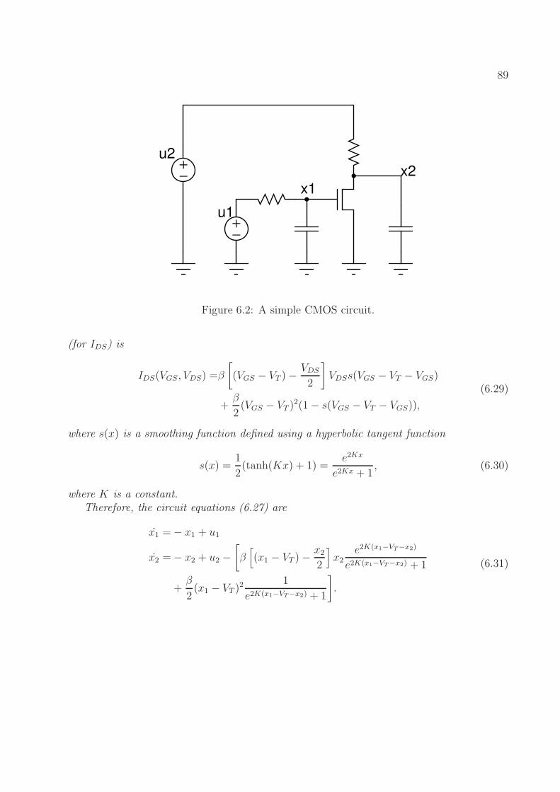
89

+

−

+

−

u1

u2

x1

x2

Figure 6.2: A simple CMOS circuit.

(for IDS) is

IDS(VGS, VDS) =β

[

(VGS − VT )−VDS

2

]

VDSs(VGS − VT − VGS)

+β

2(VGS − VT )

2(1− s(VGS − VT − VGS)),

(6.29)

where s(x) is a smoothing function defined using a hyperbolic tangent function

s(x) =1

2(tanh(Kx) + 1) =

e2Kx

e2Kx + 1, (6.30)

where K is a constant.Therefore, the circuit equations (6.27) are

x1 =− x1 + u1

x2 =− x2 + u2 −[

β[

(x1 − VT )−x2

2

]

x2e2K(x1−VT−x2)

e2K(x1−VT−x2) + 1

+β

2(x1 − VT )

2 1

e2K(x1−VT−x2) + 1

]

.

(6.31)

90

To polynomialize (6.31), we introduce two new variables

y1 = e2K(x1−VT−x2)

y2 =1

y1 + 1,

(6.32)

and add differential equations for y1 and y2. We then obtain a polynomial system

x1 =− x1 + u1

x2 =− x2 + u2 −[

β[

(x1 − VT )−x2

2

]

x2y1y2 +β

2(x1 − VT )

2y2

]

.

y1 =2Ke2K(x1−VT−x2)(x1 − x2) = 2Ky1(x1 − x2)

y2 =−1

(1 + y1)2y1 = −y22 y1.

(6.33)

Remark The polynomialization of a nonlinear system is not unique. In fact, there shouldexist a minimum-size polynomial system that corresponds to the original system. Thealgorithm to find this minimum-size polynomial system could be devised by symbolic com-putational tools. Methods in logic synthesis might also be applicable.

Despite the non-uniqueness, however, as long as the existence and uniqueness conditionsof solutions to differential equations are satisfied, the polynomial system is equivalent tothe original system since they have the same solution.

Formally, suppose the original DAEs have state variables x. We define new variablesy = g(x), and expand the DAEs by adding differential equations for y. Let x(0) be the ini-tial condition of the original DAEs, and (x(0), y(0)) be the initial condition of the expandedDAEs. If y(0) = g(x(0)) and x(t) is the solution to the original DAEs, then (x(t), g(x(t))) isthe solution to the expanded DAEs. Moreover, if the expanded DAEs satisfy the existenceand uniqueness condition of solutions, (x(t), g(x(t))) is also the unique solution.

After the polynomialization, we obtain (6.16), a polynomial system of order M . Now wepresent two approaches to convert a polynomial system (6.16) to a QLDAE system (6.8).

6.3.5 Quadratic-Linearization by Adding Quadratic Algebraic Equa-

tions

Similar to the polynomialization procedure, we iteratively define new variables y, suchthat

y = xβ1

1 · · ·xβN

N /x (6.34)

is satisfied. In (6.34), x is a variable chosen from the state variables of the expanded systemat each iteration – they include all the original state variables, as well as the newly added

91

state variables up to that iteration. We then replace xβ1

1 · · ·xβN

N in original equations by yx,and we add (6.34) into the original system. The equations in the form of (6.34) are thenre-written as quadratic algebraic equations, if possible, and are added to the original system.


x = x3 + u(t). (6.35)

To quadratic-linearize (6.35), we introduce a new variable y = x2 (i.e., x = x in (6.34)),and add it as a quadratic equation. The resulting quadratic-linear equations are

x = xy + u

0 = y − x2.(6.36)

Similar to the polynomialization procedure, quadratic-linearization procedure also pre-serves the linearity to the inputs u. Besides, we prove in the following theorem that apolynomial system can always be quadratic-linearized by adding quadratic algebraic equa-tions. As a byproduct, the theorem also provides an upper bound on the size of the QLDAEsystem derived from a polynomial system.

Theorem 6.3.8 For a polynomial system of order M , the maximum number of state vari-ables in the resulting QLDAE system does not exceed the number of state variables of

[xT , (xT ) 2©, (xT ) 3©, · · · , (xT )(⌈M2⌉)]T , by adding quadratic algebraic equations,

Proof Let y = [xT , (xT ) 2©, · · · , (xT ) p©]T , p ∈ Z+, then QLDAEs in y can generate any

nonlinear functions of the formG1y+G2y⊗y, which is essentially all the polynomial functionsin x of order not greater than 2p.

So, M ≤ 2p, i.e., p = ⌈M2⌉.

6.3.6 Quadratic-Linearization by Taking Lie Derivatives

Similarly, taking Lie derivatives of polynomial functions preserves the linearity to theinput u, and it can also lead to a QLDAE system, as proved in Theorem 6.3.9. However,the theoretical upper bound on the size of the resulting QLDAE system is more than thatby adding quadratic algebraic equations.

Theorem 6.3.9 For a polynomial system of order M , the maximum number of state vari-ables in the resulting QLDAE system does not exceed the number of state variables of

[xT , (xT ) 2©, (xT ) 3©, · · · , (xT )M© ]T , by adding differential equations that are derived by takingLie derivatives of changed variables.

92

Proof Let y = xi11 · · ·xiN

N , where∑N

k=1 ik ≤M . Then, y ∈ [xT , (xT ) 2©, (xT ) 3©, · · · , (xT )M© ]T .The differential equation of y is derived by taking its Lie derivative

d

dt(xi1

1 · · ·xiNN ) = Lx(x

i11 · · ·xiN

N )

=N∑

k=1

xi11 · · · ikxik−1

i

(

d

dtxi

)

· · ·xikN .

(6.37)

Since ddtxi is a polynomial function of maximum order M in x and linear in u, therefore

from (6.37), Lx(xi11 · · ·xiN

N ) is a polynomial function of maximum order 2M − 1 in x and

linear in u, i.e., this is a QLDAE system in [xT , (xT ) 2©, · · · , (xT )M©]T .

6.3.7 Quadratic-Linearization Algorithm

As a summary, we present the quadratic-linearization algorithm for polynomial ODEsin Algorithm 7, which quadratic-linearizes a polynomial system of order M in the form of(6.16) where ci,i = 1 and ci,j = 0, ∀i 6= j.

The computational complexity of Algorithm 7 is polynomial with respect to the orderof the polynomial system, because the size of the equivalent quadratic-linear system is apolynomial function of the order of the polynomial system.

6.3.8 Polynomialization and Quadratic-Linearization of DAEs

More generally, systems may be modeled by differential algebraic equations in the formof

d

dt(q(x)) = f(x) +Bu. (6.38)

Similarly, we deal with equations where each element in f(x), denoted by fi(x), and eachelement in q(x), denoted by qi(x), are summations of elementary functions, i.e.,

fi(x) =gi,1(x) + · · ·+ gi,ki(x),

qi(x) =hi,1(x) + · · ·+ hi,li(x),(6.39)

where ki, li are constant integers denoting the number of nonlinear functions in fi and qi,respectively.

93

Algorithm 7 Quadratic-Linearization of Polynomial ODEs

Inputs: E = [x1, · · · , xn], the list of symbolic expressions of the polynomial ODEs.Outputs: Yvar, the set of new variables;Yexpr, the set of expressions of new variables;E, the list of symbolic expressions of the QLDAEs.

1: Initialize Yvar ← , Yexpr ← ;2: repeat3: From E, the list of symbolic expressions of the ODEs, pick a monomial m(x) that has

degree > 2 (in terms of x and variables in Yvar).4: Find a decomposition of m(x), i.e., find g(x) and h(x) that satisfy m(x) = g(x)×h(x).5: Define a new state variable y = g(x).6: Add y into Yvar, and g(x) into Yexpr.7: Compute the symbolic expression of y = g′(x)x.8: Add the symbolic expression of y to E.9: for all monomials m(x) in E do10: if m(x) is linear or quadratic in terms of x and variables in Yvar then11: Replace m(x) as a linear or quadratic term.12: end if13: end for14: until All expressions in E are linear or quadratic functions of x and variables in Yvar.

Polynomialization

The polynomialization procedure is similar to the ODE case. We first introduce newvariables

yi,1 = gi,1(x), · · · , yi,ki = gi,ki(x),

zi,1 = hi,1(x), · · · , zi,li = hi,li(x).(6.40)

Therefore, (6.38) is converted to

d

dt(zi,1 + · · ·+ zi,li) = yi,1 + · · ·+ yi,ki + biu, i = 1, · · · , N. (6.41)

If equations in (6.40) can be written in the polynomial form, we can simply add them aspolynomial equations.

If equations in (6.40) cannot be written in the polynomial form, we add the differential

94

equations

d

dtyi,1 = g′i,1(x)

d

dtx, · · · , d

dtyi,ki = g′i,ki(x)

d

dtx,

d

dtzi,1 = h′

i,1(x)d

dtx, · · · , d

dtzi,li = h′

i,li(x)

d

dtx.

(6.42)

However, we may not have explicit expressions for ddtx, and we do not reach a polynomial

system in the form of (6.16). We therefore extend the definition of a polynomial system tobe the following:

Definition 6.3.2 (Generalized polynomial system) The generalized polynomial systemis defined to be of the form (6.43), and it is said to be of order M , if the highest order of

monomial of x is M , i.e., M = maxk,i

(

∑Nj=1 ζi,k,l,j,

∑Nl=1 βi,k,l,

∑Nl=1 γi,k,l

)

.

∑

l

[

∑

k

ξi,k,lxζi,k,l,11 · · ·xζi,k,l,N

N

]

xl

=∑

k

αi,kxβi,k,1

1 · · ·xβi,k,N

N +

(

∑

k

ηi,kxγi,k,11 · · ·xγi,k,N

N

)

u

i = 1, · · · , N, ζi,k,l,j ≥ 0, βi,k,j ≥ 0, γi,k,j ≥ 0,

ζi,k,l,j ∈ Z, βi,k,j ∈ Z, γi,k,j ∈ Z, ∀k, j, l.

(6.43)

With this new definition, and following the proof of 6.3.4, it is straightforward that DAEscan be converted to a generalized polynomial system.

Quadratic-Linearization

Similarly, we extend the definition of QLDAEs to a more general form

d

dt[C1x+ C2x⊗ x] = G1x+G2x⊗ x+ (D1x+D2x⊗ x)u+Bu. (6.44)

Similar to the proof of Theorems 6.3.8 and 6.3.9, it is easy to show that by addingquadratic algebraic equations and differential equations, we can convert a generalized poly-nomial system (6.43) to a generalized QLDAE system (6.44).

6.4 QLMOR

In this section, we focus on the reduction step for QLDAEs (6.8). Similar, but morecomplicated derivations can be performed for generalized QLDAEs (6.44).

95

We start by performing a variational analysis to show the validity of applying Krylov-subspace methods. We then derive the moments of transfer functions of (6.8), which providesa guideline of how to choose the proper Krylov subspace for generating a smallest reducedmodel in the sense of moment-matching. The derivations in this section unifies previousworks on polynomial systems and bilinear systems [106, 107].

6.4.1 Variational Analysis

The variational analysis [105] starts by assuming the QLDAE system is a combinationof a series of homogeneous nonlinear sub-systems, whose responses to u(t) are x1(t), x2(t),etc.. That is, when input is αu(t), the response x(t) is

x(t) = αx1(t) + α2x2(t) + α3x3(t) + α4x4(t) + · · · . (6.45)

Therefore, by inserting (6.45) into (6.8), and equating the terms corresponding to αi, i =1, 2, · · · , we obtain

Cd

dtx1 =G1x1 +Bu,

Cd

dtx2 =G1x2 +G2x1 ⊗ x1 +D1x1u,

Cd

dtx3 =G1x3 +G2(x1 ⊗ x2 + x2 ⊗ x1) +D1x2u+D2(x1 ⊗ x1)u,

Cd

dtx4 =G1x4 +G2(x1 ⊗ x3 + x2 ⊗ x2 + x3 ⊗ x1)

+D1x3u+D2(x1 ⊗ x2 + x2 ⊗ x1)u.

(6.46)

From (6.46), if in the i-th set of differential equations (i.e., equations where LHS is ddtxi),

we lump the terms without xi to be pseudo inputs, then the original system can be viewed asa series of linear systems. Therefore, the Krylov subspace that guarantees that the projectedsystem matches the moments of these linear systems is K(G−1

1 C,G−11 ([B,G2, D1, D2])), if G1

is non-singular. However, the size of this subspace can easily exceed the size of the originalsystem. Therefore, care must be taken to choose a useful subspace.

6.4.2 Matrix Transfer Functions

Following [105], we can show that transfer functions for (6.8) can be written as follows.(Only first three transfer functions are listed.)

H1(s) = (sC −G1)−1B, (6.47)

96

H2(s1, s2) =((s1 + s2)C −G1)−1

1

2

[

G2(H1(s1)⊗H1(s2) +H1(s2)⊗H1(s1))

+D1(H1(s1) +H2(s2))

]

,

(6.48)

H3(s1, s2, s3)

=((s1 + s2 + s3)C −G1)−1

1

6

G2

[

H1(s1)⊗H2(s2, s3) +H1(s2)⊗H2(s1, s3)

+H1(s3)⊗H2(s1, s2) +H2(s2, s3)⊗H1(s1)

+H2(s1, s3)⊗H1(s2) +H2(s1, s2)⊗H1(s3)

]

+D1

[

H2(s1, s2) +H2(s2, s3) +H2(s1, s3)

]

+D2

[

H1(s1)⊗H1(s2) +H1(s1)⊗H1(s3) +H1(s2)⊗H1(s1)

+H1(s2)⊗H1(s3) +H1(s3)⊗H1(s1) +H1(s3)⊗H1(s2)

]

.

(6.49)

Based on (6.47), (6.48) and (6.49), the Taylor expansion of these transfer functions can bederived. Correspondingly, we obtain the moments of the transfer functions, i.e., coefficientsof sk for H1(s), s

k1s

l2 for H2(s1, s2), etc.. For example,

H1(s) =

∞∑

k=0

M1,ksk =

∞∑

k=0

AkR1sk

H2(s) =∞∑

k=0

∞∑

l=0

M2,k,lsk1s

l2 =

∞∑

k=0

AkR1(s1 + s2)kG−1

1

1

2

G2

[

(

∞∑

k=0

AkR1sk1

)

⊗(

∞∑

k=0

AkR1sk2

)

+

(

∞∑

k=0

AkR1sk2

)

⊗(

∞∑

k=0

AkR1sk1

)

]

+D1

[

∞∑

k=0

AkR1sk2 +

∞∑

k=0

AkR1sk2

]

,

(6.50)

97

where A = G−11 C, R1 = −G−1

1 B, and M1,k, M2,k,l are the moments for H1(s) and H2(s1, s2),respectively. Similar derivations can be performed for higher order moments.

An interesting point to note is that H2(s1, s2) is the same as the summation of theH2(s1, s2) of a bilinear system C d

dtx = G1x +D1xu + Bu and the H2(s1, s2) of a quadratic

system C ddtx = G1x+G2x⊗ x+Bu.

6.4.3 Subspace Basis Generation for Moment Matching

To illustrate how QLMOR generates the projection matrix, we derive the theorem andalgorithm for H2(s1, s2) in the following. These derivations can be easily extended for higher-order moment-matching.

From (6.50), we can derive the vectors that are the coefficients for an n-th order moment.(E.g., forH2(s1, s2), the n-th order moments refers to the set of coefficients for sk1s

l2, k+l = n.)

As an example, those vectors forH2(s1, s2) are listed in Table 6.3. We then have the followingtheorem:

Theorem 6.4.1 Given a QLDAE system (6.8), suppose

R(V ) =AiR1, i ≤ q⋃

AiG−11 D1A

jR1, i+ j ≤ q⋃

AiG−11 G2(A

jR1)⊗ (AkR1), i+ j + k ≤ q, k ≤ j(6.51)

Then if

x = V xr, Cr = V TCV, Br = V TB,

Gr,1 = V TG1V, Gr,2 = V TG2V ⊗ V,

Dr,1 = V TD1V, Dr,2 = V TD2V ⊗ V,

(6.52)

the reduced system (6.53) matches the moments of H2(s1, s2) of the original system up toq-th order.

Crd

dtxr = Gr,1xr +Gr,2xr ⊗ xr +Dr,1xru+Dr,2(xr ⊗ xr)u+Bru (6.53)

Proof The proof is similar to that in [106].

Notice that the second and the third set of basis vectors in Theorem 6.4.1 count forthe moments of the corresponding bilinear system and quadratic system, respectively – thisresult also follows from the above theorem by setting G2 = D2 = 0 and D1 = D2 = 0 in theQLDAE system.

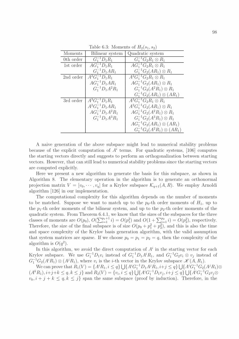
98

Table 6.3: Moments of H2(s1, s2)

Moments Bilinear system Quadratic system0th order G−1

1 D1R1 G−11 G2R1 ⊗R1

1st order AG−11 D1R1 AG−1

1 G2R1 ⊗R1

G−11 D1AR1 G−1

1 G2(AR1)⊗R1

2nd order A2G−11 D1R1 A2G−1

1 G2R1 ⊗R1

AG−11 D1AR1 AG−1

1 G2(AR1)⊗R1

G−11 D1A

2R1 G−11 G2(A

2R1)⊗ R1

G−11 G2(AR1)⊗ (AR1)

3rd order A3G−11 D1R1 A3G−1

1 G2R1 ⊗R1

A2G−11 D1AR1 A2G−1

1 G2(AR1)⊗R1

AG−11 D1A

2R1 AG−11 G2(A

2R1)⊗ R1

G−11 D1A

3R1 G−11 G2(A

3R1)⊗ R1

AG−11 G2(AR1)⊗ (AR1)

G−11 G2(A

2R1)⊗ (AR1)

A naive generation of the above subspace might lead to numerical stability problemsbecause of the explicit computation of Ai terms. For quadratic systems, [106] computesthe starting vectors directly and suggests to perform an orthogonalization between startingvectors. However, that can still lead to numerical stability problems since the starting vectorsare computed explicitly.

Here we present a new algorithm to generate the basis for this subspace, as shown inAlgorithm 8. The elementary operation in the algorithm is to generate an orthonormalprojection matrix V = [v0, · · · , vq] for a Krylov subspace Kq+1(A,R). We employ Arnoldialgorithm [126] in our implementation.

The computational complexity for this algorithm depends on the number of momentsto be matched. Suppose we want to match up to the p0-th order moments of H1, up tothe p1-th order moments of the bilinear system, and up to the p2-th order moments of thequadratic system. From Theorem 6.4.1, we know that the sizes of the subspaces for the threeclasses of moments are O(p0), O(

∑p1+1i=1 i) = O(p21) and O(1 +

∑p2i=1 i) = O(p22), respectively.

Therefore, the size of the final subspace is of size O(p0 + p21 + p22), and this is also the timeand space complexity of the Krylov basis generation algorithm, with the valid assumptionthat system matrices are sparse. If we choose p0 = p1 = p2 = q, then the complexity of thealgorithm is O(q2).

In this algorithm, we avoid the direct computation of Ai in the starting vector for eachKrylov subspace. We use G−1

1 D1vi instead of G−11 D1A

iR1, and G−11 G2vi ⊗ vj instead of

G−11 G2(A

iR1)⊗ (AjR1), where vi is the i-th vector in the Krylov subspace K (A,R1).We can prove thatR1(V ) = AiR1, i ≤ q

⋃

AiG−11 D1A

jR1, i+j ≤ q⋃

AiG−11 G2(A

jR1)⊗(AkR1), i+j+k ≤ q, k ≤ j andR2(V ) = vi, i ≤ q

⋃

AiG−11 D1vj , i+j ≤ q

⋃

AiG−11 G2vj⊗

vk, i + j + k ≤ q, k ≤ j span the same subspace (proof by induction). Therefore, in the

99

computation of the starting vector, no Ai terms are involved.We can also prove that vi1⊗vj1 is orthogonal to vi2⊗vj2 if i1 6= i2 or j1 6= j2 (by definition of

Kronecker product). Hence, the starting vectors have better numerical properties than [106].However, it is not always the case that G−1

1 G2vi1 ⊗ vj1 is orthogonal to G−11 G2vi2 ⊗ vj2, even

if vi1 ⊗ vj1 is orthogonal to vi2 ⊗ vj2 . Therefore, one further improvement of this algorithmis to perform an orthonormalization of the starting vector to the basis already generated.

Proofs are omitted here due to page limits.

Algorithm 8 Generation of basis for subspace in Theorem 6.4.1

Inputs: C,G1, G2, D1, D2 matrices defining the QLDAEs;q: the reduced model will match up to the q-th order moments of H1 and H2.Outputs: V : the projection matrix.

1: A = G−11 C, R1 = −G−1

1 B.2: Generate matrix V = [v0, · · · , vq] for Kq+1(A,R1)3: for i = 0 to q do4: Generate matrix W = [w0, · · · , wq−i]

for Kq−i+1(A,G−11 D1vi). subspace for moments of the bilinear system

5: V = qr([V,W ]).6: end for7: for i = 0 to q do8: for j = 0 to min(q − i, i) do9: Generate matrix W = [w0, · · · , wq−i−j] for Kq−i−j+1(A,G

−11 G2vi ⊗ vj). subspace

for moments of the quadratic system10: V = qr([V,W ]).11: end for12: end for

6.4.4 Discussion on Local Passivity Preservation

The loss of passivity in [106, 107, 121] are mainly caused by Taylor approximation. QL-MOR alleviates this problem in the sense that the conversions to the polynomial system andthe quadratic-linear system are exact, and no passivity loss is introduced in that step.

In the reduction step, however, the passivity may again be lost. One may show that ourreduced model linearized at any xr,0 ∈ R

Nr , is a congruence transformation of the originalsystem linearized at x0 = V xr,0 ∈ R

N . Under somewhat strict conditions such as the onesin [11], the passivity of the linearized system can be preserved.

100

6.4.5 Discussion on Constructing Appropriate QLDAEs

As mentioned in Section 6.3, different QLDAE formulations are all equivalent. How-ever, the reduced QLDAEs are generally not equivalent. We discuss how different QLDAEformulations lead to different reduced models.

Consider a nonlinear system,

d

dtx = f(x) +Bu, (6.54)

from which we can derive QLDAEs

d

dtxq = G1xq +G2xq ⊗ xq +D1xqu+D2xq ⊗ xqu+Bu, (6.55)

where the state variables are xq = (x, y) where y = g(x) are nonlinear functions of x.According to Theorem 6.4.1, by choosing appropriate projection matrices, we can match

the first few moments of (x, y). Therefore, by formulating different QLDAEs where differenty’s are added, the moments of different y’s are matched in different reduced models. Thisresult is of great importance in practice – depending on the output signal, which is a nonlinearfunction of state variables, we may compute reduced models that matches moments of theseoutput signals.

There is another subtle but important guideline of choosing new state variables – onlyadd variables y = g(x) so that yDC = g(xDC) = 0 where xDC is the DC solution of (6.54) foru = uDC. (Without loss of generality, we assume that xDC = 0.)

To see why this is useful, we consider two QLDAEs that are equivalent to (6.54), and arein terms of xα and xβ, respectively:

d

dtxα = G1,αxα +G2,αxα ⊗ xα +D1,αxαu+D2,αxα ⊗ xαu+Bαu, (6.56)

d

dtxβ = G1,βxβ +G2,βxβ ⊗ xβ +D1,βxβu+D2,βxβ ⊗ xβu+Bβu. (6.57)

The state variables xα and xβ satisfy 1) xα = 0 when u = uDC; 2) xβ = xα + x0, wherex0 is a non-zero constant vector.

Generally, G1,α 6= G1,β, G2,α 6= G2,β, D1,α 6= D1,β, D2,α 6= D2,β, Bα 6= Bβ . Thereforethe moments of two QLDAEs are not the same. This, however, does not imply that thetwo QLDAEs are not equivalent. Rather, loosely speaking, it implies that the moments ofsystems “quadratic-linearized around different states” are not the same.

To see that, we note that G1,α is the Jacobian matrix of RHS of (6.56) computed atxα = 0 = xα,DC , and G1,β is the Jacobian matrix of RHS of (6.57) computed at xβ = 0.However, when u = uDC , xβ = xα+x0 = x0 6= 0. Therefore, in order to match moments of theoriginal system (6.54) around xDC , it is inappropriate to use G1,β in moment computations,

101

and it is inappropriate to use (6.57) in QLMOR.Rather, we can show that the moments of (6.56) linearized around 0 match the moments of

(6.54) linearized around xDC , thus leading to the guideline of choosing y such that yDC = 0.The proof of this result involves a bit linear algebra, but is quite straightforward, and isomitted here.

6.4.6 Computational Cost of Simulation of the Reduced Model

The computational cost of simulating a dynamical system is composed of two parts:function (including Jacobian) evaluation and linear solve.

The quadratic-linear reduced models only involve quadratic nonlinearities, and thereforethe function computation only involves multiplications, and the Jacobian matrix is a linearfunction of x. This is an advantage over previous higher-order reduced models, as well ascomplex models that involve expensive exponential function computations and complicatedflow-control statements. Additionally, because the size of the model is Nr (much smallerthan N), the linear solve is also expected to be much faster.

However, there is one important source that slows down the computation – the sparsityof the system is destroyed in the reduced models. It is not easy to estimate how this sparsity-loss affect the computational cost, but in practice we observe speedups of reduced modelsover original models.

Compared to trajectory-based methods, our reduced model has a more tractable com-putational cost for the function and Jacobian evaluations. Assuming that we have Nr statevariables in the reduced model, the function evaluation is bounded by O(N3

r ) multiplica-tions (assuming the worst case where there are O(N2

r ) quadratic terms for q equations);the complexity of Jacobian matrix evaluation is O(N2

r ) because it is a linear function ofstate variables. On the other hand, trajectory-based methods try to compute V Tf(V xr) byusing interpolation among sample points stored in the reduced model. To obtain a modelwith high-fidelity, however, a very large number of sample points need to be stored, and thecomputation can become very slow.

6.4.7 Multi-Point Expansion

The multi-point Krylov subspace method [127] can be directly applied in QLMOR, andit potentially leads to a smaller and more accurate model for a specified frequency range ofinterest.

Also note that the quadratic-linearization procedure in Section 6.3 might render a QL-DAE system where G1 is singular. This can be a potential problem for generating Krylovsubspaces at s = 0. The current workaround for this problem is to generate Krylov subspacesat s = s0, s0 ≃ 0.

102


In this section, we illustrate the applicability of the QLMOR method presented in theprevious sections, demonstrating its efficiency and accuracy on example circuits and systems.

6.5.1 A System with a x1+x Nonlinearity

As noted in Section 6.3, x, x⊗x and xK+x

are common nonlinearities in biochemical rateequations. To test how QLMOR works, a random second-order polynomial system with ax

1+xfunction was generated to mimic a biochemical reaction system4:

d

dtx+G1x+G2x⊗ x+ e1

10x1

1 + x1

+Bu = 0. (6.58)

The size of (6.58) is 10, hence G1 ∈ R10×10, G2 ∈ R

10×100, B ∈ R10×1, e1 ∈ R

10×1 =[1, 0, · · · , 0]T . Notice that we manually make G1 dense, non-symmetric, and make its eigen-values uniformly distributed. Those factors all make MOR for this system more difficultthan for many real systems that are normally sparse and symmetric.

To compare with the QLMOR method, we first show that Taylor-expansion based meth-ods [106, 107] are not applicable. The Taylor series of the function 1

1+xis

1

1 + x=

∞∑

i=0

(−x)i = 1− x+ x2 − x3 + x4 − x5 + · · · , (|x| < 1). (6.59)

Notice that (6.59) converges only when |x| < 1 (also clearly seen in Fig. 6.3), making theTaylor approximation irrelevant and highly inaccurate for |x| ≥ 1; as a result, any reducedmodel derived from this approximation cannot be accurate for |x| ≥ 1. Indeed, the Taylorapproximation model turns out to be an unstable system for polynomial orders from 2 to7, i.e., the polynomial model has a finite escape time [73]. As mentioned in [107], suchapproximations do not preserve properties such as stability and passivity, except by chance.

To apply the QLMOR method, we perform quadratic-linearization of the original systemby making the variable change y = x1

1+x1. Following the procedure in Section 6.3, we obtain

a QLDAE system equivalent to (6.58):

d

dtx+G1x+G2x⊗ x+ e110y +Bu = 0,

−x1 + y + x1y = 0.(6.60)

4The eigenvalues of G1 were manipulated to be positive such that the linearized system at 0 is stable. Theeigenvalues are uniformly sampled on [0, 20]. G2 was made sparse (5% non-zeros), which is approximatelyof the same order in real rate equations and circuit equations. The coefficient in front of x1

1+x1

were madelarge enough to make the system exhibit high nonlinearity.

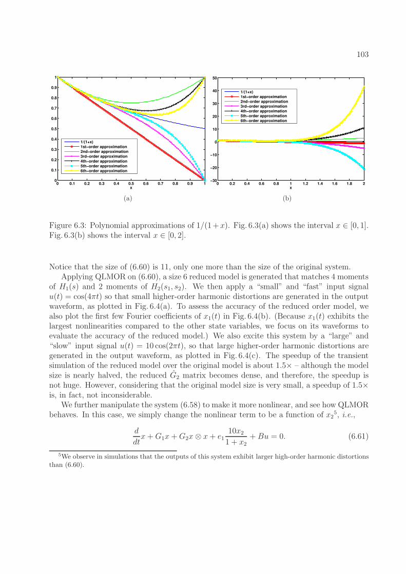
103

0 0.1 0.2 0.3 0.4 0.5 0.6 0.7 0.8 0.9 10

0.1

0.2

0.3

0.4

0.5

0.6

0.7

0.8

0.9

1

x

1/(1+x)

1st−order approximation

2nd−order approximation

3rd−order approximation

4th−order approximation



(a)

0 0.2 0.4 0.6 0.8 1 1.2 1.4 1.6 1.8 2−30

−20

−10

0

10

20

30

40

50

x

1/(1+x)

1st−order approximation

2nd−order approximation

3rd−order approximation




(b)

Figure 6.3: Polynomial approximations of 1/(1+x). Fig. 6.3(a) shows the interval x ∈ [0, 1].Fig. 6.3(b) shows the interval x ∈ [0, 2].

Notice that the size of (6.60) is 11, only one more than the size of the original system.Applying QLMOR on (6.60), a size 6 reduced model is generated that matches 4 moments

of H1(s) and 2 moments of H2(s1, s2). We then apply a “small” and “fast” input signalu(t) = cos(4πt) so that small higher-order harmonic distortions are generated in the outputwaveform, as plotted in Fig. 6.4(a). To assess the accuracy of the reduced order model, wealso plot the first few Fourier coefficients of x1(t) in Fig. 6.4(b). (Because x1(t) exhibits thelargest nonlinearities compared to the other state variables, we focus on its waveforms toevaluate the accuracy of the reduced model.) We also excite this system by a “large” and“slow” input signal u(t) = 10 cos(2πt), so that large higher-order harmonic distortions aregenerated in the output waveform, as plotted in Fig. 6.4(c). The speedup of the transientsimulation of the reduced model over the original model is about 1.5× – although the modelsize is nearly halved, the reduced G2 matrix becomes dense, and therefore, the speedup isnot huge. However, considering that the original model size is very small, a speedup of 1.5×is, in fact, not inconsiderable.

We further manipulate the system (6.58) to make it more nonlinear, and see how QLMORbehaves. In this case, we simply change the nonlinear term to be a function of x2

5, i.e.,

d

dtx+G1x+G2x⊗ x+ e1

10x2

1 + x2

+Bu = 0. (6.61)

5We observe in simulations that the outputs of this system exhibit larger high-order harmonic distortionsthan (6.60).

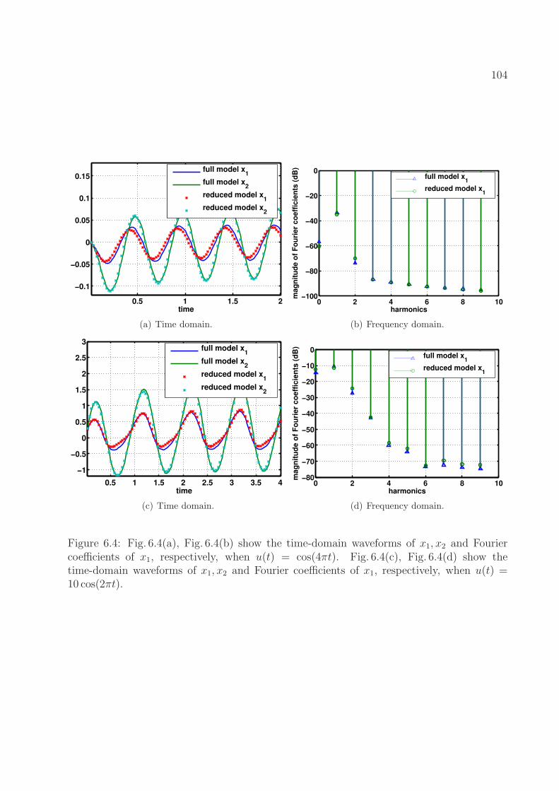
104

0.5 1 1.5 2

−0.1

−0.05

0

0.05

0.1

0.15

time

full model x1

full model x2

reduced model x1

reduced model x2

(a) Time domain.

0 2 4 6 8 10−100

−80

−60

−40

−20

0

harmonics

mag

nit

ud

e o

f F

ou

rier

co

eff

icie

nts

(d

B)

full model x1

reduced model x1

(b) Frequency domain.

0.5 1 1.5 2 2.5 3 3.5 4

−1

−0.5

0

0.5

1

1.5

2

2.5

3

time

full model x1

full model x2

reduced model x1

reduced model x2

(c) Time domain.

0 2 4 6 8 10−80

−70

−60

−50

−40

−30

−20

−10

0

harmonics

ma

gn

itu

de

of

Fo

uri

er

co

eff

icie

nts

(d

B)

full model x1

reduced model x1

(d) Frequency domain.

Figure 6.4: Fig. 6.4(a), Fig. 6.4(b) show the time-domain waveforms of x1, x2 and Fouriercoefficients of x1, respectively, when u(t) = cos(4πt). Fig. 6.4(c), Fig. 6.4(d) show thetime-domain waveforms of x1, x2 and Fourier coefficients of x1, respectively, when u(t) =10 cos(2πt).

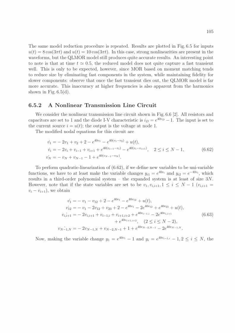
105

The same model reduction procedure is repeated. Results are plotted in Fig. 6.5 for inputsu(t) = 8 cos(3πt) and u(t) = 10 cos(3πt). In this case, strong nonlinearities are present in thewaveforms, but the QLMOR model still produces quite accurate results. An interesting pointto note is that at time t ≃ 0.5, the reduced model does not quite capture a fast transientwell. This is only to be expected, however, since MOR based on moment matching tendsto reduce size by eliminating fast components in the system, while maintaining fidelity forslower components: observe that once the fast transient dies out, the QLMOR model is farmore accurate. This inaccuracy at higher frequencies is also apparent from the harmonicsshown in Fig. 6.5(d).

6.5.2 A Nonlinear Transmission Line Circuit

We consider the nonlinear transmission line circuit shown in Fig. 6.6 [2]. All resistors andcapacitors are set to 1 and the diode I-V characteristic is iD = e40vD − 1. The input is set tothe current source i = u(t); the output is the voltage at node 1.

The modified nodal equations for this circuit are

v1 =− 2v1 + v2 + 2− e40v1 − e40(v1−v2) + u(t),

vi =− 2vi + vi−1 + vi+1 + e40(vi−1−vi) − e40(vi−vi+1), 2 ≤ i ≤ N − 1,

˙vN =− vN + vN−1 − 1 + e40(vN−1−vN ).

(6.62)

To perform quadratic-linearization of (6.62), if we define new variables to be uni-variablefunctions, we have to at least make the variable changes yi1 = e40vi and yi2 = e−40vi , whichresults in a third-order polynomial system – the expanded system is at least of size 3N .However, note that if the state variables are set to be v1, vi,i+1, 1 ≤ i ≤ N − 1 (vi,i+1 =vi − vi+1), we obtain

v1 =− v1 − v12 + 2− e40v1 − e40v12 + u(t),

˙v12 =− v1 − 2v12 + v23 + 2− e40v1 − 2e40v12 + e40v23 + u(t),

˙vi,i+1 =− 2vi,i+1 + vi−1,i + vi+1,i+2 + e40vi−1,i − 2e40vi,i+1

+ e40vi+1,i+2 , (2 ≤ i ≤ N − 2),

˙vN−1,N =− 2vN−1,N + vN−2,N−1 + 1 + e40vN−2,N−1 − 2e40vN−1,N .

(6.63)

Now, making the variable change y1 = e40v1 − 1 and yi = e40vi−1,i − 1, 2 ≤ i ≤ N , the

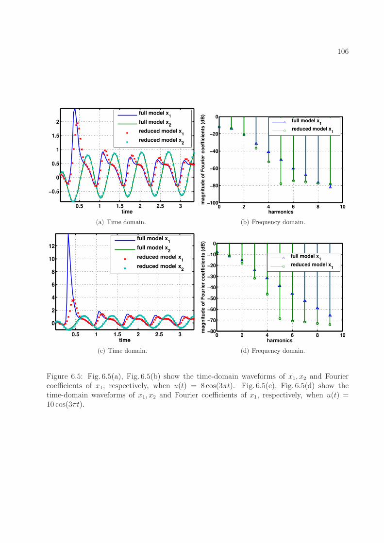
106

0.5 1 1.5 2 2.5 3

−0.5

0

0.5

1

1.5

2

time

full model x1

full model x2

reduced model x1

reduced model x2

(a) Time domain.

0 2 4 6 8 10−100

−80

−60

−40

−20

0

harmonics

mag

nit

ud

e o

f F

ou

rier

co

eff

icie

nts

(d

B)

full model x1

reduced model x1


0.5 1 1.5 2 2.5 3

0

2

4

6

8

10

12

time

full model x1

full model x2

reduced model x1

reduced model x2

(c) Time domain.

0 2 4 6 8 10−80

−70

−60

−50

−40

−30

−20

−10

0

harmonics

ma

gn

itu

de

of

Fo

uri

er

co

eff

icie

nts

(d

B)

full model x1

reduced model x1

(d) Frequency domain.

Figure 6.5: Fig. 6.5(a), Fig. 6.5(b) show the time-domain waveforms of x1, x2 and Fouriercoefficients of x1, respectively, when u(t) = 8 cos(3πt). Fig. 6.5(c), Fig. 6.5(d) show thetime-domain waveforms of x1, x2 and Fourier coefficients of x1, respectively, when u(t) =10 cos(3πt).

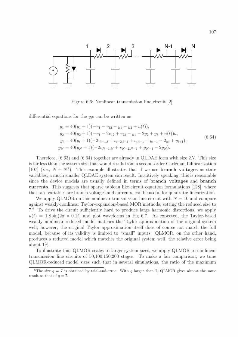
107

......

1 2 3 NN-1

Figure 6.6: Nonlinear transmission line circuit [2].

differential equations for the yis can be written as

y1 = 40(y1 + 1)(−v1 − v12 − y1 − y2 + u(t)),

y2 = 40(y2 + 1)(−v1 − 2v12 + v23 − y1 − 2y2 + y3 + u(t))a,

yi = 40(yi + 1)(−2vi−1,i + vi−2,i−1 + vi,i+1 + yi−1 − 2yi + yi+1),

˙yN = 40(yN + 1)(−2vN−1,N + vN−2,N−1 + yN−1 − 2yN).

(6.64)

Therefore, (6.63) and (6.64) together are already in QLDAE form with size 2N . This sizeis far less than the system size that would result from a second-order Carleman bilinearization[107] (i.e., N + N2). This example illustrates that if we use branch voltages as statevariables, a much smaller QLDAE system can result. Intuitively speaking, this is reasonablesince the device models are usually defined in terms of branch voltages and branchcurrents. This suggests that sparse tableau like circuit equation formulations [128], wherethe state variables are branch voltages and currents, can be useful for quadratic-linearization.

We apply QLMOR on this nonlinear transmission line circuit with N = 10 and compareagainst weakly-nonlinear Taylor-expansion-based MOR methods, setting the reduced size to7.6 To drive the circuit sufficiently hard to produce large harmonic distortions, we applyu(t) = 1.8 sin(2π × 0.1t) and plot waveforms in Fig. 6.7. As expected, the Taylor-basedweakly nonlinear reduced model matches the Taylor approximation of the original systemwell; however, the original Taylor approximation itself does of course not match the fullmodel, because of its validity is limited to “small” inputs. QLMOR, on the other hand,produces a reduced model which matches the original system well, the relative error beingabout 1%.

To illustrate that QLMOR scales to larger system sizes, we apply QLMOR to nonlineartransmission line circuits of 50,100,150,200 stages. To make a fair comparison, we tuneQLMOR-reduced model sizes such that in several simulations, the ratio of the maximum

6The size q = 7 is obtained by trial-and-error. With q larger than 7, QLMOR gives almost the sameresult as that of q = 7.

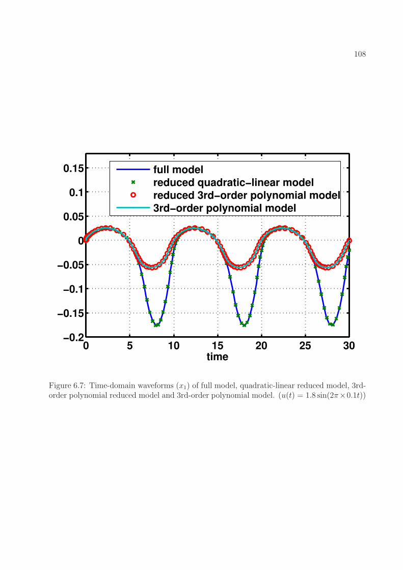
108

0 5 10 15 20 25 30−0.2

−0.15

−0.1

−0.05

0

0.05

0.1

0.15

time

full model

reduced quadratic−linear model

reduced 3rd−order polynomial model

3rd−order polynomial model

Figure 6.7: Time-domain waveforms (x1) of full model, quadratic-linear reduced model, 3rd-order polynomial reduced model and 3rd-order polynomial model. (u(t) = 1.8 sin(2π×0.1t))

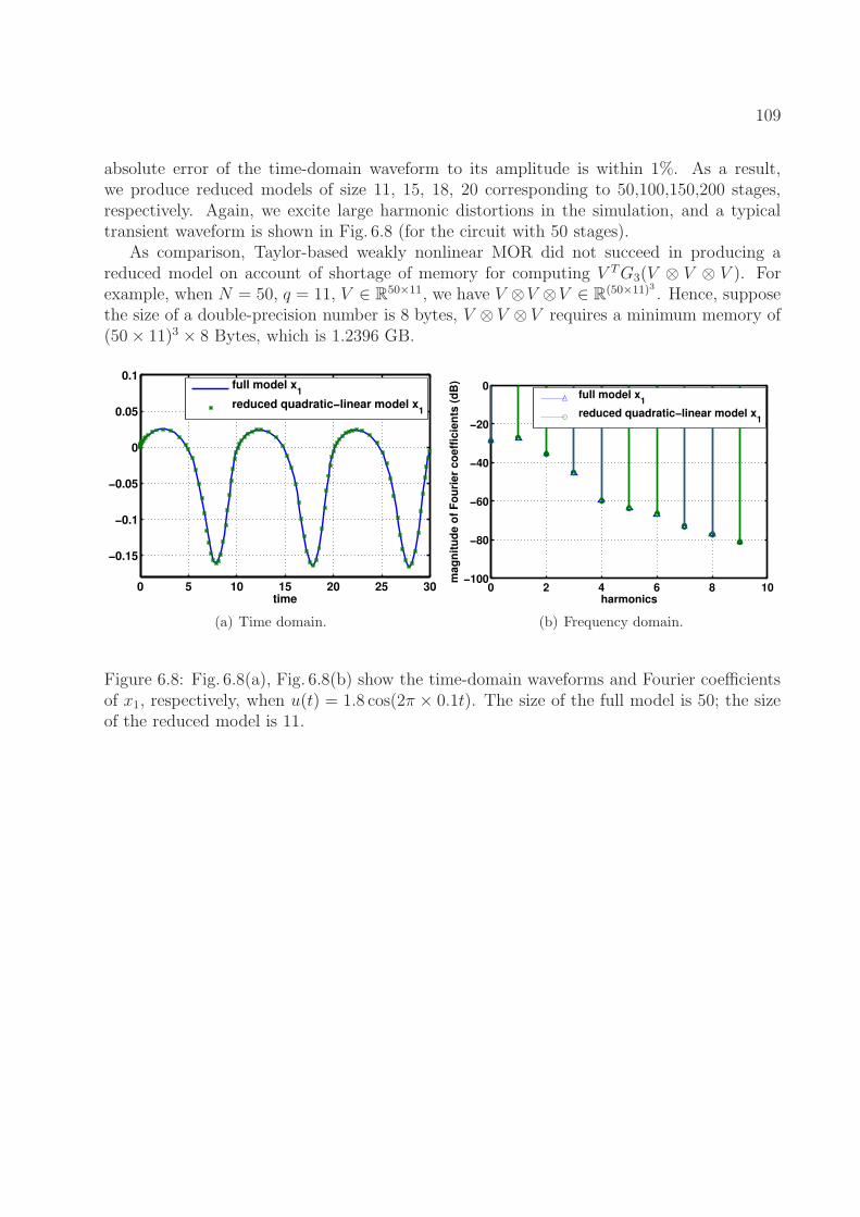
109

absolute error of the time-domain waveform to its amplitude is within 1%. As a result,we produce reduced models of size 11, 15, 18, 20 corresponding to 50,100,150,200 stages,respectively. Again, we excite large harmonic distortions in the simulation, and a typicaltransient waveform is shown in Fig. 6.8 (for the circuit with 50 stages).

As comparison, Taylor-based weakly nonlinear MOR did not succeed in producing areduced model on account of shortage of memory for computing V TG3(V ⊗ V ⊗ V ). Forexample, when N = 50, q = 11, V ∈ R

50×11, we have V ⊗V ⊗V ∈ R(50×11)3 . Hence, suppose

the size of a double-precision number is 8 bytes, V ⊗ V ⊗ V requires a minimum memory of(50× 11)3 × 8 Bytes, which is 1.2396 GB.

0 5 10 15 20 25 30

−0.15

−0.1

−0.05

0

0.05

0.1

time

full model x1

reduced quadratic−linear model x1

(a) Time domain.

0 2 4 6 8 10−100

−80

−60

−40

−20

0

harmonics

mag

nit

ud

e o

f F

ou

rier

co

eff

icie

nts

(d

B)

full model x1

reduced quadratic−linear model x1


Figure 6.8: Fig. 6.8(a), Fig. 6.8(b) show the time-domain waveforms and Fourier coefficientsof x1, respectively, when u(t) = 1.8 cos(2π × 0.1t). The size of the full model is 50; the sizeof the reduced model is 11.

110

Chapter 7

NTIM: Phase/Timing Macromodeling

In this chapter, we present a special macromodeling technique that captures phase re-sponses of nonlinear systems. While the phase response is yet to be defined, it can beintuitively thought of as timing behaviors such as delay or phase modulation, and thereforeis an extremely important behavior in many practical systems, especially in circuits.

We formally define the phase response and discuss its applications. We derive a phasemacromodel via a nonlinear perturbation analysis, and present numerical methods to com-pute the phase macromodel. We show its applications in modeling circuits and neurons, andcompare the results with the full model in terms of accuracy and computational cost.

7.1 Phase Response and its Applications

In many systems, due to design intents or physical constraints, the waveforms of statevariables are almost the same, and therefore can be characterized by the phase information.For example: in phase modulation circuits, we aim to design a system that transformsthe input signal u(t) and a carrier signal x(t) to a output signal y(t) = x(t + u(t)). Indigital circuits, outputs of waveforms typically saturate at the power supply voltages, andthe waveforms all look like a ramp waveform, either from “0” to “1” or from “1” to “0”.However, the exact shape of waveforms are not the same under different input signals, andthese shapes may be characterized by the point-to-point delay information, or equivalentlythe phase information.

In fact, using phase information alone, we may represent a very rich set of waveforms.

Example 7.1.1 Suppose x(t) = sin(2πt), and

y(t) = x(t+ z(t)) = sin(2π(t+ z(t))) (7.1)

By choosing z(t) carefully, y(t) can represent a very rich set of waveforms. As shown inFig. 7.1,

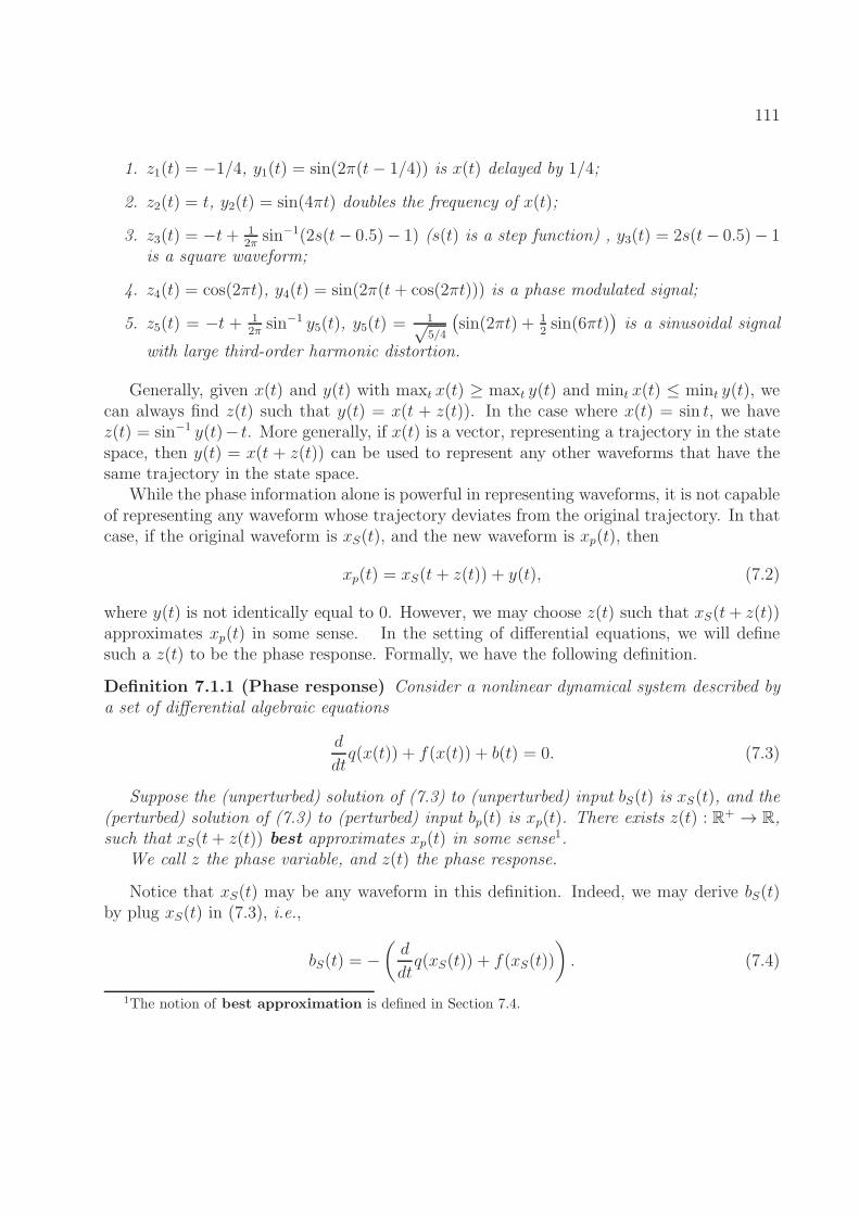
111

1. z1(t) = −1/4, y1(t) = sin(2π(t− 1/4)) is x(t) delayed by 1/4;

2. z2(t) = t, y2(t) = sin(4πt) doubles the frequency of x(t);

3. z3(t) = −t+ 12π

sin−1(2s(t− 0.5)− 1) (s(t) is a step function) , y3(t) = 2s(t− 0.5)− 1is a square waveform;

4. z4(t) = cos(2πt), y4(t) = sin(2π(t+ cos(2πt))) is a phase modulated signal;

5. z5(t) = −t + 12π

sin−1 y5(t), y5(t) =1√5/4

(

sin(2πt) + 12sin(6πt)

)

is a sinusoidal signal

with large third-order harmonic distortion.

Generally, given x(t) and y(t) with maxt x(t) ≥ maxt y(t) and mint x(t) ≤ mint y(t), wecan always find z(t) such that y(t) = x(t + z(t)). In the case where x(t) = sin t, we havez(t) = sin−1 y(t)− t. More generally, if x(t) is a vector, representing a trajectory in the statespace, then y(t) = x(t + z(t)) can be used to represent any other waveforms that have thesame trajectory in the state space.

While the phase information alone is powerful in representing waveforms, it is not capableof representing any waveform whose trajectory deviates from the original trajectory. In thatcase, if the original waveform is xS(t), and the new waveform is xp(t), then

xp(t) = xS(t+ z(t)) + y(t), (7.2)

where y(t) is not identically equal to 0. However, we may choose z(t) such that xS(t+ z(t))approximates xp(t) in some sense. In the setting of differential equations, we will definesuch a z(t) to be the phase response. Formally, we have the following definition.

Definition 7.1.1 (Phase response) Consider a nonlinear dynamical system described bya set of differential algebraic equations

d

dtq(x(t)) + f(x(t)) + b(t) = 0. (7.3)

Suppose the (unperturbed) solution of (7.3) to (unperturbed) input bS(t) is xS(t), and the(perturbed) solution of (7.3) to (perturbed) input bp(t) is xp(t). There exists z(t) : R+ → R,such that xS(t+ z(t)) best approximates xp(t) in some sense1.

We call z the phase variable, and z(t) the phase response.

Notice that xS(t) may be any waveform in this definition. Indeed, we may derive bS(t)by plug xS(t) in (7.3), i.e.,

bS(t) = −(

d

dtq(xS(t)) + f(xS(t))

)

. (7.4)

1The notion of best approximation is defined in Section 7.4.

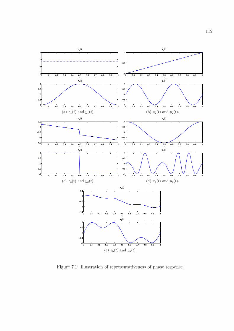
112

0 0.1 0.2 0.3 0.4 0.5 0.6 0.7 0.8 0.9 1−2

−1

0

1

t

z1(t)

0 0.1 0.2 0.3 0.4 0.5 0.6 0.7 0.8 0.9 1−1

−0.5

0

0.5

1

y1(t)

(a) z1(t) and y1(t).

0 0.1 0.2 0.3 0.4 0.5 0.6 0.7 0.8 0.9 10

0.5

1

t

z2(t)

0 0.1 0.2 0.3 0.4 0.5 0.6 0.7 0.8 0.9 1−1

−0.5

0

0.5

1

y2(t)

(b) z2(t) and y2(t).

0 0.1 0.2 0.3 0.4 0.5 0.6 0.7 0.8 0.9 1−1.5

−1

−0.5

0

0.5

t

z3(t)

0 0.1 0.2 0.3 0.4 0.5 0.6 0.7 0.8 0.9 1−1

−0.5

0

0.5

1

y3(t)

(c) z3(t) and y3(t).

0 0.1 0.2 0.3 0.4 0.5 0.6 0.7 0.8 0.9 1−1

−0.5

0

0.5

1

t

z4(t)

0 0.1 0.2 0.3 0.4 0.5 0.6 0.7 0.8 0.9 1−1

−0.5

0

0.5

1

y4(t)

(d) z4(t) and y4(t).

0 0.1 0.2 0.3 0.4 0.5 0.6 0.7 0.8 0.9 1−1.5

−1

−0.5

0

0.5

t

z5(t)

0 0.1 0.2 0.3 0.4 0.5 0.6 0.7 0.8 0.9 1−1

−0.5

0

0.5

1

y5(t)

(e) z5(t) and y5(t).

Figure 7.1: Illustration of representativeness of phase response.

113

This definition can also be understood from a geometrical view point. As shown inFig. 7.22, the solid (blue) orbit is the trajectory to input bS(t), and the dotted (red) orbit isthe trajectory to input bp(t). At time t, on the orbit of xS(t), there exists a point given byxS(t+ z(t)) which best approximates xp(t) on the perturbed orbit. The remaining differencey(t) = xp(t) − xS(t + z(t)) is called the amplitude deviation [29]. Therefore, we canview the response to input bp(t) as combined effects of the phase response and the amplitudedeviation, i.e.,

xp(t) = xS(t+ z(t)) + y(t). (7.5)

Figure 7.2: Illustration of phase response.

Remark This definition is dependent on the trajectory of xS(t), and therefore bS(t). There-fore, it may be called a xS-PR (phase response).

With this definition of phase response, it is worth noting that although the phase responseis an important characteristic of oscillators as pioneered by many researchers [29, 129], it is

2We show two closed orbits in Fig. 7.2 for simplicity, but there is no restriction of the orbit being closedin our definition. The orbit can be arbitrary.

114

not a special characteristic only for oscillators, but generally for all kinds of dynamicalsystems. It has broader applications in many fields.

Phase response is of great importance in circuits in particular. For examples, in os-cillators, phase noise or timing jitter is the phase response in a stochastic setting wherenoise/uncertainties are present; in digital gates and RC interconnects, timing informationsuch as delay and slope is essentially derived from the phase response; in a pulse generator,the pulse width can also be derived from the phase response.

Scientists in biology and neuroscience also place a great emphasis on quantitative under-standing of the phase response. For examples, normal human circadian rhythm disorders,which can be caused by insomnia, fatigue and jet lag, are phase responses of underlyingphysiological processes under different perturbations; synchronization of a neural network isa phenomenon where the phase responses of all neurons settle down to the same value; someneuron firing/bursting behaviors, which are exhibited when currents are injected, can alsobe understood as the phase response of the neuron.

7.2 Phase Macromodels

With the above definition of the phase response, the phase macromodel is a model thatdescribes the dynamics of the phase response. In another word, the phase macromodel iscomposed of a differential equation in terms of z(t), and therefore is a 1-dimensional reducedorder model.

To use the phase macromodel, we simulation the differential equation for z(t), instead of(7.3), and use xS(t+ z(t)) to approximate the original solution xp(t). With the assumptionthat y(t) is small, xS(t+ z(t)) will give a very good approximation to xp(t).

In many systems, the validity of this assumption depends on both the system propertiesas well as input perturbations. Fortunately, we see a lot of applications that this assumptionis satisfied. For examples: in oscillators that are asymptotically orbital stable, the periodicorbit is an attractor which by definition attracts all trajectories nearby; in digital appli-cations, although circuits never reside in a periodic steady state, their trajectories followalmost the same path since inputs are basically signals switching between “0” and “1” withvariations of the slope, to the first-order approximation.

Among all possible perturbations, there is also a special one that is very useful andnormally makes the above assumption satisfied. This is the phase perturbation, i.e., theperturbed input bp(t) = bS(t + p(t)) is only a phase-modulated version of bS(t) by somesignal p(t). For example, it can be used to represent an FM/PM signal in RF applications,or a delayed ramp signal with any slope in digital applications. In particular, when p(t)is a constant, the perturbed solution xp(t) lies exactly on the same orbit of xS(t) if initialcondition is set properly.

115

7.3 Preliminaries and Notations (of LPTV systems)

To understand derivations in the following sections, we need to introduce a few notationsand lemmas. For simplicity, we consider the system defined by a set of ordinary differentialequations

d

dtx(t) = f(x(t)) + b(t). (7.6)

Following [130], the results can be extended to differential algebraic equations.We assume that the input b(t) is a periodic signal bS(t) with period T , and that under

this input, the asymptotic response of the system is xS(t) which is also periodic with periodT .

A traditional perturbation analysis using linearization can then be carried out: assumingthat the response to the perturbed input bp(t) = bS(t) + bw(t) is xp(t) = xS(t) + w(t), andsubstituting xp(t) and bp(t) in (7.6), we obtain

d

dt(xS(t) + w(t)) = f (xS(t) + w(t)) + (bS(t) + bw(t)) . (7.7)

To the first order approximation, we have

d

dtw(t) = G(t)w(t) + bw(t), (7.8)

where G(t) = ∂f∂x

∣

∣

xS(t)is a time-varying matrix with period T .

(7.8) is an LPTV system, whose solution, according to Floquet theory [131], is

w(t) =Φ(t, 0)w0 +

∫ t

0

Φ(t, s)bw(s)ds

=U(t)D(t)V T (0)w0 + U(t)

∫ t

0

D(t− s)V T (s)bw(s)ds

=

n∑

i=1

ui(t)eµitvTi (0)w0 +

n∑

i=1

ui(t)

∫ t

0

eµi(t−s)vTi (s)bw(s)ds

=n∑

i=1

ui(t)

(

eµitvTi (0)w0 +

∫ t

0

eµi(t−s)vTi (s)bw(s)ds

)

,

(7.9)

where w0 is the initial condition for (7.8), Φ(t, s) = U(t)D(t − s)V T (s) is the state tran-sition matrix of (7.8), µis are the Floquet exponents, D(t) = diag(eµ1t, · · · , eµnt), U(t) =[u1(t), · · · , un(t)], V (t) = [v1(t), · · · , vn(t)], and V T (t)U(t) = In. More theories and proofsabout LPTV systems can be found in [131].

We now introduce a lemma showing that dxS(t)dt

, the time derivative of the periodic solution

116

xS(t) of (7.6), satisfies an LPTV system.

Lemma 7.3.1 The time derivative of the periodic solution xS(t) of (1.2), i.e., ddt(xS(t))

satisfiesd

dtw(t) = G(t)w(t) +

dbS(t)

dt, (7.10)

and can be written asdxS

dt(t) = U(t)c(t) =

N∑

i=1

ui(t)ci(t), (7.11)

where

ci(t) = limr=t+kT,k→∞

(

eµirvTi (0)dxS

dt(0) +

∫ r

0

eµi(r−s)vTi (s)

(

d

dsbS(s)

)

ds

)

. (7.12)

Proof Since xS(t) satisfies (7.6), we have

d

dtxS(t) = f(xS(t)) + bS(t). (7.13)

Take the time derivative of (7.13) on both sides, we obtain

d

dt

(

dxS(t)

dt

)

=d

dt(f(xS(t)) + bS(t)) =

∂f

∂x

∣

∣

∣

∣

xS(t)

dxS(t)

dt+

dbS(t)

dt. (7.14)

Therefore, ddt(xS(t)) satisfies (7.10).

Since ddtxS(t) is the asymptotic periodic solution to (7.10), according to (7.9), we further

have (7.11) with c(t) defined by (7.12).

7.4 Derivation of the Phase Macromodel via Nonlinear

Perturbation Analysis

With the important assumption that the trajectory of the perturbed system stays closeto the trajectory of xS(t), the key idea is to show that under the perturbed input bp(t), theperturbed response xp(t) can be decomposed into the phase response z(t) and the amplitudedeviation y(t) in a reasonable way, i.e.,

xp(t) = xS(t+ z(t)) + y(t), (7.15)

and that by defining the right differential equation for z(t), y(t) is minimized in some sense.

117

To show this, we start by defining the phase equation, i.e., the differential equation forthe phase response z(t). We then show that the input bp(t) can be decomposed into bz(t)and by(t) such that when only bz(t) is applied to (7.6), the perturbed response is exactlyxS(t + z(t)). We then derive the first-order approximation of y(t) by linearizing originaldifferential equations around the phase-shifted solution xS(t + z(t)), and show that certaindecomposition of y(t) is minimized.

Definition 7.4.1 (Phase Equation) We define the phase equation to be

cT (t+ z)c(t + z)dz

dt= cT (t+ z)V T (t+ z) [bp(t)− bS(t+ z)] , (7.16)

where c(t) = [c1(t), · · · , cN(t)] is defined in (7.12) and V (t) is defined in (7.9).

With the definition of z(t), we present a theorem showing that part of the input bp(t)contributes only to the phase response.

Theorem 7.4.1 Given any perturbed input ~bp(t), define

bz(t) =bS(t+ z) +cT (t + z)

cT (t+ z)c(t + z)V T (t + z)

· [bp(t)− bS(t+ z)]U(t+ z)c(t + z),

(7.17)

then xS(t+ z(t)) is the solution to

d

dt(x(t)) = f(x(t)) + bz(t). (7.18)

Proof Substituting xS(t+ z(t)) in (7.18), we have

d

dt[xS(t+ z(t))] = f(xS(t + z(t))) + bz(t)

=dxS

dt(t + z(t))

(

1 +dz

dt

)

.(7.19)

Substituting (7.11) in (7.19), and defining τ = t + z, we have

f(xS(τ)) + bS(τ) + U(τ)c(τ)dz

dt= f(xS(τ)) + bz(t)

U(τ)c(τ)dz

dt= bz(t)− bS(τ).

(7.20)

118

Substituting (7.17) in (7.20), we have

U(τ)c(τ)dz

dt=

[

cT (τ)

cT (τ)c(τ)V T (τ)(bp(t)− bS(τ))

]

U(τ)c(τ). (7.21)

Since U(τ)c(τ) is dxS

dt(τ) whose elements are not simultaneously zero, we obtain (7.16). Since

all above derivations are reversible, we have also shown that xS(t+ z(t)) solves (7.18).

It remains to show that by decomposing the perturbed response xp(t) into phase responseand amplitude deviation according to (7.16), the amplitude deviation is minimized in somesense. This is proven by the following theorem. The proof also gives another derivation ofthe phase equation (7.16).

Theorem 7.4.2 Suppose the perturbed response is xp(t) = xS(t + z(t)) + y(t), then to thefirst-order approximation, y(t) is

y(t) = U(τ)

∫ τ

0

eΛ(t−s)r(s)ds, (7.22)

where τ = t + z, Λ = diag(µ1, · · · , µn) are the Floquet exponents of (7.8), and y(t) isminimized in the sense that ||r(s)||2 is minimized.

Proof We first assume that the response to bz(t) is exactly xS(t + z), which gives

d

dtxS(t+ z(t)) =

dxS

dτ(τ)(1 +

dz

dt)

=f(x(τ)) + bS(τ) +dxS

dτ(τ)

d

dtz(t).

(7.23)

Suppose the phase equation is dzdt

= a(t), then

bz(t) = bS(t+ z) + a(t)dxS

dt(t+ z). (7.24)

Now substituting xp(t) = xS(t+ z) + y(t) into (1.2), we have

d

dt(xS(t + z) + y(t)) = f(xS(t+ z) + y(t)) + bp(t)

≃f(xS(t+ z)) +G(t+ z)y(t) + bz(t) + [bp(t)− bz(t))] .(7.25)

Therefore, we have

d

dty(t) = G(t + z)y(t) + [bp(t)− bz(t)] . (7.26)

119

With the assumption that dzdt

is small [29], we define t = t + z, y(t) = y(t), bw(t) =bp(t)− bz(t), and therefore

d

dty(t) = G(t)y(t) + bw(t). (7.27)

Therefore, applying (7.9), we have

y(t) = y(t) = U(t)

∫ t

0

eΛ(t−s)V T (s)bw(s)ds, (7.28)

Therefore, r(t) in (7.22) is

r(t) =V T (t)bw(t)

=V T (t+ z) (bp(t)− bS(t+ z)− a(t)U(t + z)c(t + z))

=V T (t+ z) (bp(t)− bS(t+ z))− a(t)c(t + z).

(7.29)

The minimization of ||r(t)||2 boils down to the problem of minimizing ||Ax− b||2 whereA = c(t+ z), x = a(t) and b = V T (t+ z) [bp(t)− bS(t+ z)]. The solution to this problem issimply

a(t) =cT (t + z)

cT (t+ z)c(t + z)V T (t + z)(bp(t)− bS(t+ z)), (7.30)

which again leads to (7.16).

7.4.1 Interpretation in the Projection Framework

The model shown in Section 7.4 can be interpreted as a special reduced order model inthe projection framework mentioned in Chapter 4, where state variables are forced to liein an Nr-dimensional manifold defined by x = v(xr), and the residual is forced to lie in aNr-dimensional manifold defined by rz = w(rx).

To derive the same phase macromodel under the projection framework, we first enforcethat the perturbed response xp(t) only induces a phase shift, i.e., the state variable lie on thesame orbit as that of the unperturbed solution. This is equivalent to saying that we projectthe state space onto the one-dimensional manifold defined by the unperturbed solution xS(t)which has a natural parameterization by time t. Therefore, the projection function is definedby

x(t) = v(z(t)) = xS(t + z). (7.31)


d

dtxS(t+ z) =f(xS(t+ z)) + bp(t). (7.32)

120

Therefore,

d

dt[xS(t+ z)] =

dxS

dτ(τ)

dτ

dt=

dxS

dτ(τ)

(

1 +dz

dt

)

=dxS

dτ(τ) +

dxS

dτ(τ)

dz

dt.

(7.33)

On the other hand, we have

d

dτxS(τ) = f(xS(τ)) + bS(τ), (7.34)

and therefore, (7.33) can be written as

d

dtxS(t+ z) =f(xS(τ)) + bS(τ) +

d

dτxS(τ)

dz

dt. (7.35)

Combining (7.32) and (7.35), we obtain

d

dτxS(τ)

dz

dt= bp(t)− bS(τ), (7.36)

or equivalently,

U(τ)c(τ)dz

dt= bp(t)− bS(τ). (7.37)

Therefore, after the projection onto the periodic orbit, we obtain N equations (7.37) and1 state variable z. To derive a reduced order model, we further project the residual, i.e.,(7.37), to a one-dimensional manifold. In our model, we have chosen the projection to be

w(rx) = cT (τ)V T (τ)rx, (7.38)

which is shown to minimize the amplitude deviation in the sense of Theorem 7.4.2.

7.4.2 Connections to PPV Macromodel

The PPV phase macromodel [29] is specifically devised to characterize the phase responseof an oscillatory system. Its limitation is that it is only applicable to oscillators. Thisexcludes it from wide applications such as traditional timing analysis and excitory firingneuron network simulations.

Following previous derivations, the PPV macromodel is indeed a special case of ourgeneral-purpose phase macromodel. We can obtain the PPV model for oscillators by choosingc(t) in (7.16) to be [1, 0, · · · , 0]T .

This choice of c(t) in fact is the definition in (7.12) for autonomous oscillators. To seethat, we note that for autonomous oscillators, the following two conditions are satisfied: (1)

121

one Floquet exponent of (7.10) to be 0 and others negative (e.g., µ1 = 0, µi < 0, 2 ≤ i ≤ n),and (2) bS(t) is constant. Therefore, (7.12) becomes

c1(t) = limt→∞

~vTi (0)d~xS

dt(0) = 1,

ci(t) = limt→∞

eµit~vTi (0)d~xS

dt(0) = 0, 2 ≤ i ≤ n.

(7.39)

which leads to c(t) = [1, 0, · · · , 0]T , and the PPV model.

7.4.3 Generalization for Non-Periodic Trajectories

Previous derivations are based on the assumption that xS(t) is the asymptotic periodicorbit in the state space. This is not generally the case for practical systems such as digitalcircuits. However, if we force the input to be a periodic signal (for example, a squarewave), then the system will converge to a periodic steady state, and transient behaviors (forexample, the rising and falling edge of waveforms) are well-approximated by its periodicsteady state. Hence, we can force the input to be periodic as long as the periodic trajectorywell-approximates the non-periodic ones. As a result, the derived phase model will alsocharacterize the transient phase responses.

7.5 Algorithm

Based on the above analysis, the algorithm to generate a general-purpose phase macro-model is shown as follows.

Algorithm 9 General-Purpose Phase Macromodeling

1: Given input bS(t), compute the periodic steady state xS(t).

2: Compute dxS(t)dt

, the time derivative of xS(t).3: Perform Floquet decomposition of the LPTV system

dwdt

= G(xS(t))w(t) (compute U(t), V (t), and D(t)).

4: Compute c(t) = V T (t)dxS(t)dt

.5: Precompute cT (t)c(t) and cT (t)V T (t) in (7.16) and store them in the model.

7.6 Numerical Methods for Computing the Phase Model

As shown in Algorithm 9, to compute the phase macromodel, we need to compute the pe-riodic steady state xS(t), its time derivative dxS(t)

dt, and perform a full Floquet decomposition

of an LPTV system.

122

PSS analysis has been widely adopted in commercial tools and usually uses shootingmethod [132], FDTD method [132] or harmonic balance [132]. The time derivative of thePSS solution can be computed either in the time domain directly by finite difference approx-imation or in the frequency domain and be transformed back to time domain.

The main numerical challenge lies in the Floquet decomposition, which is numericallymuch more ill-conditioned. Implementations according to textbook definitions using Mon-odromy matrix fail without question. In this section, we first demonstrate that methodsbased on explicitly computing the Monodromy matrix are numerically extremely bad. Wethen present3 two much better-behaved methods to solve this challenge, one based on har-monic balance, and the other based on finite-difference time-domain (FDTD) method.

7.6.1 Floquet Decomposition using Monodromy Matrix

We consider the Floquet decomposition of the LPTV system

d

dtx(t) +G(t)x(t) = 0. (7.40)

Floquet decomposition [131] refers to computing matrices U(t), V (t) and D = eΛt (whereΛ is a diagonal matrix of all Floquet exponents) such that the state transition matrix of(7.40) is

Φ(t, s) = U(t)D(t− s)V T (s). (7.41)

The definition for Floquet exponents are derived from the eigenvalues of themonodromymatrix defined by

B = Φ(T, 0) = PeΛTP−1, (7.42)

and U(t) is then defined as Φ(t, 0)Pe−Λt, and V (t) = U−1(t).This definition naturally gives a straightforward implementation of Floquet decomposi-

tion:

Algorithm 10 Floquet Decomposition using Monodromy Matrix

1: Starting with initial conditionX(0) = I, integrate (7.40) to compute Φ(t, 0) for t ∈ [0, T ].2: Compute the monodromy matrix B = Φ(T, 0).3: Eigen-decompose the monodromy matrix B = PeΛTP−1.4: Compute U(t) = Φ(t, 0)Pe−Λt and V (t) = U−1(t).

This algorithm will work in perfect precision. However, it almost never works in practice.For real systems, most Floquet exponents are normally negative. This means that using anyinitial condition P , the solution to (7.40) (which is Φ(t, 0)P ) tends to 0 exponentially. This

3While these methods seem to have been developed before, we present our derivation and also explainthe details in the derivation.

123

makes the computed monodromy matrix B extremely numerically singular, and the eigen-decomposition of B provides useless results. Also, computing V (t) using the inverse of U(t)is not a good choice since the smoothness of V (t) can easily be destroyed.

7.6.2 Equations in terms of U(t) and V (t)

As the first and the most important step to tackle the problems in the Monodromy matrixmethod, we derive equations whose unknowns are U(t) and V (t), respectively. Because U(t)and V (t) are periodic, the resulting differential equations have solutions that are periodic,instead of decaying to 0. Therefore, this avoids numerical errors in the Monodromy matrixcomputation. Moreover, having equations for U(t) and V (t) separately avoids computingV (t) = U−1(t).

To derive these equations, we start with a fundamental matrix

X(t) = Φ(t, 0) = U(t)D(t)V T (0), (7.43)

which solves (7.40). Substituting (7.43) in (7.40), we have

d

dt

[

U(t)D(t)V T (0)]

+G(t)U(t)D(t)V T (0) = 0

⇔ d

dt[U(t)D(t)] +G(t)U(t)D(t) = 0

⇔[

d

dtU(t)

]

eΛt + U(t)

[

d

dteΛt]

+G(t)U(t)eΛt = 0.

(7.44)

Therefore,d

dtU(t) + U(t)Λ +G(t)U(t) = 0. (7.45)

Similarly, to derive the equations for V (t), we apply the same technique to the adjointsystem of (7.40)

dy(t)

dt−GT (t)y(t) = 0, (7.46)

which has a fundamental matrix

Y (t) = V (t)D(−t)UT (0). (7.47)


d

dt(V (t)D(−t))−GT (t)V (t)D(−t) = 0

⇔(

d

dtV (t)e−Λt + V (t)(−Λ)e−Λ(t)

)

−GT (t)V (t)e−Λ(t) = 0.(7.48)

124

Therefore,d

dtV (t)− V (t)Λ−GT (t)V (t) = 0. (7.49)

Therefore, we have shown that U(t) and V (t) satisfy differential equations (7.45) and(7.49), respectively. To solve for U(t) and V (t), we note that they are by definition periodicwith period T , and therefore we need to force the their periodicity during the computation.Two numerical methods that force the periodicity are HB and FDTD, and we now show howto apply these methods to solve for U(t) and V (t).

7.6.3 Floquet Decomposition via Harmonic Balance

Notations

We follow the notations in [133]: For any periodic matrix or vector A(t) which has atruncated Fourier series A(t) =

∑Mi=−M Aie

jiωt (ω = 2πT), we define the block vector VA(t) of

Ais and the block-Toeplitz matrix TA(t) of Ais to be

VA(t) =

...A2

A1

A0

A−1

A−2...

, TA(t) =

......

......

...· · · A0 A1 A2 A3 A4 · · ·· · · A−1 A0 A1 A2 A3 · · ·· · · A−2 A−1 A0 A1 A2 · · ·· · · A−3 A−2 A−1 A0 A1 · · ·· · · A−4 A−3 A−2 A−1 A0 · · ·

......

......

...

. (7.50)

Using this notation, two lemmas follow [133]:

Lemma 7.6.1 If Z(t) = X(t)Y (t), and X(t), Y (t) are T -periodic, then,

VZ(t) = TX(t)VY (t), VZT (t) = TY T (t)VXT (t),

TZ(t) = TX(t)TY (t), TZT (t) = TY T (t)VXT (t).(7.51)

Lemma 7.6.2 If X(t) is T -periodic, then

VX(t) = ΩVX(t), TX(t) = ΩTX(t) − TX(t)Ω, (7.52)

where Ω = Ω0 ⊗ In, Ω0 = jωdiag(· · · , 2, 1, 0,−1,−2, · · · ). (7.53)

125

HB for Floquet decomposition

Theorem 7.6.3 The eigenvalues and eigenvectors of the HB Jacobian matrix for (7.40)(JHB = Ω+ TG(t)) are given by the diagonal of Ω0 ⊗ In − I2M+1 ⊗ Λ and TU(t), respectively.

The eigenvalues and eigenvectors of the HB Jacobian matrix for (7.46) (JHB = Ω−TGT (t))are given by the diagonal of Ω0 ⊗ In + I2M+1 ⊗ Λ and TV (t), respectively.

Proof Applying lemmas 7.6.1 and 7.6.2 to to (7.45), we have

ΩTU(t) − TU(t)Ω+ TU(t)TΛ + TG(t)TU(t) = 0

⇔ (Ω + TG(t))TU(t) + TU(t)(TΛ − Ω) = 0,(7.54)

which is already in the eigen-decomposed form of JHB = Ω + TG(t).Similarly, applying lemmas 7.6.1 and 7.6.2 to to (7.49), we have

(ΩTV (t) − TV (t)Ω)− TV (t)TΛ − TGT (t)TV (t) = 0

⇔ (Ω− TGT (t))TV (t) − TV (t)(Ω + TΛ) = 0,(7.55)

which is already in the eigen-decomposed form of JHB = Ω− TGT (t).

Therefore, solving for U(t) and V (t) boils down to the matrix eigenvalue problem of JHB

and JHB. To pick up the right eigenvectors for U(t) and V (t), we note that eigenvalues oftwo matrices are λi,k = jiω ∓ µk,−M ≤ i ≤ M, 1 ≤ k ≤ n. and the block vector VU(t) andVV (t) correspond to eigenvalues λ0,k = µk. Therefore, assuming µks are real, we can pick upthe eigenvectors corresponding to real eigenvalues to obtain VU(t) and VV (t). This leads tothe following algorithm:

Algorithm 11 Floquet Decomposition via Harmonic Balance

1: Construct Jacobian matrices JHB and JHB in Thm. 7.6.3.2: Eigen-decompose JHB and JHB.3: Select real eigenvalues to be the Floquet exponents µks, and eigenvectors corresponding

to µks to be VU(t) and VV (t).4: Perform inverse FFT to compute U(t) and V (t) in time-domain.

126

7.6.4 Floquet Decomposition via FDTD Method

Notations

Given any T -periodic matrix or vector A(t), sampled at N time points t0, · · · , tN−1, wedenote block vector VA(t) and the block diagonal matrix DA(t) to be

VA(t) =

A(t0)A(t1)...

A(tN−1)

, DA(t) =

A(t0)A(t1)

. . .

A(tN−1)

. (7.56)

Using these notations, two lemmas follow [133]:

Lemma 7.6.4 If Z(t) = X(t)Y (t), and X(t), Y (t) are T -periodic, then,

VZ(t) = DX(t)VY (t), DZ(t) = DX(t)DY (t). (7.57)

Lemma 7.6.5 If X(t) is T -periodic, then

VX(t) = ΩTDVx(t), (7.58)

where ΩTD depends on different finite difference schemes.

ΩTD = HΩ0,TD ⊗ In, H = diag(1

h0, · · · , 1

hN−1). (7.59)

For example, Ω0,TD for backward Euler and central difference schemes are

Ω0,BE =

1 −1−1 1

. . .. . .

−1 1

, Ω0,CE =

0 1 −1−1 0 1

. . .. . .

. . .

−1 0 1

. (7.60)

FDTD for Floquet decomposition

Theorem 7.6.6 The diagonal of −Λ and VU(t) are n eigenvalues and eigenvectors of theFDTD Jacobian matrix for (7.40) (JFDTD = ΩTD + TG(t)), and the diagonal of Λ and

VV (t) are n eigenvalues and eigenvectors of the FDTD Jacobian matrix for (7.46) (JFDTD =ΩTD − TGT (t)).

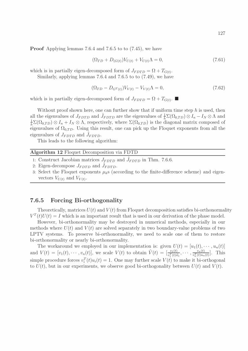
127

Proof Applying lemmas 7.6.4 and 7.6.5 to to (7.45), we have

(ΩTD +D(G(t))VU(t) + VU(t)Λ = 0, (7.61)

which is in partially eigen-decomposed form of JFDTD = Ω + TG(t).Similarly, applying lemmas 7.6.4 and 7.6.5 to to (7.49), we have

(ΩTD −DGT (t))VV (t) − VV (t)Λ = 0, (7.62)

which is in partially eigen-decomposed form of JFDTD = Ω + TG(t).

Without proof shown here, one can further show that if uniform time step h is used, thenall the eigenvalues of JFDTD and JFDTD are the eigenvalues of 1

hΣ(Ω0,TD)⊗ In− IN ⊗Λ and

1hΣ(Ω0,TD)⊗ In + IN ⊗ Λ, respectively, where Σ(Ω0,TD) is the diagonal matrix composed of

eigenvalues of Ω0,TD. Using this result, one can pick up the Floquet exponents from all the

eigenvalues of JFDTD and JFDTD.This leads to the following algorithm:

Algorithm 12 Floquet Decomposition via FDTD

1: Construct Jacobian matrices JFDTD and JFDTD in Thm. 7.6.6.2: Eigen-decompose JFDTD and JFDTD.3: Select the Floquet exponents µks (according to the finite-difference scheme) and eigen-

vectors VU(t) and VV (t).

7.6.5 Forcing Bi-orthogonality

Theoretically, matrices U(t) and V (t) from Floquet decomposition satisfies bi-orthonormalityV T (t)U(t) = I which is an important result that is used in our derivation of the phase model.

However, bi-orthonormality may be destroyed in numerical methods, especially in ourmethods where U(t) and V (t) are solved separately in two boundary-value problems of twoLPTV systems. To preserve bi-orthonormality, we need to scale one of them to restorebi-orthonormality or nearly bi-orthonormality.

The workaround we employed in our implementation is: given U(t) = [u1(t), · · · , un(t)]

and V (t) = [v1(t), · · · , vn(t)], we scale V (t) to obtain V (t) = [ v1(t)

vT1(t)~u1

, · · · , vn(t)vTn (t)un(t)

]. This

simple procedure forces vTi (t)ui(t) = 1. One may further scale V (t) to make it bi-orthogonalto U(t), but in our experiments, we observe good bi-orthogonality between U(t) and V (t).

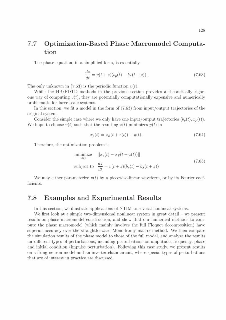
128

7.7 Optimization-Based Phase Macromodel Computa-

tion

The phase equation, in a simplified form, is essentially

dz

dt= v(t+ z)(bp(t)− bS(t+ z)). (7.63)

The only unknown in (7.63) is the periodic function v(t).While the HB/FDTD methods in the previous section provides a theoretically rigor-

ous way of computing v(t), they are potentially computationally expensive and numericallyproblematic for large-scale systems.

In this section, we fit a model in the form of (7.63) from input/output trajectories of theoriginal system.

Consider the simple case where we only have one input/output trajectories (bp(t), xp(t)).We hope to choose v(t) such that the resulting z(t) minimizes y(t) in

xp(t) = xS(t+ z(t)) + y(t). (7.64)

Therefore, the optimization problem is

minimizev(t)

||xp(t)− xS(t+ z(t))||

subject todz

dt= v(t+ z)(bp(t)− bS(t+ z))

(7.65)

We may either parameterize v(t) by a piecewise-linear waveform, or by its Fourier coef-ficients.


In this section, we illustrate applications of NTIM to several nonlinear systems.We first look at a simple two-dimensional nonlinear system in great detail – we present

results on phase macromodel construction, and show that our numerical methods to com-pute the phase macromodel (which mainly involves the full Floquet decomposition) havesuperior accuracy over the straightforward Monodromy matrix method. We then comparethe simulation results of the phase model to those of the full model, and analyze the resultsfor different types of perturbations, including perturbations on amplitude, frequency, phaseand initial condition (impulse perturbation). Following this case study, we present resultson a firing neuron model and an inverter chain circuit, where special types of perturbationsthat are of interest in practice are discussed.

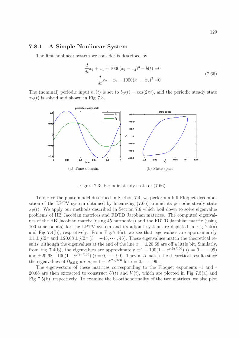
129

7.8.1 A Simple Nonlinear System

The first nonlinear system we consider is described by

d

dtx1 + x1 + 1000(x1 − x2)

3 − b(t) =0

d

dtx2 + x2 − 1000(x1 − x2)

3 =0.

(7.66)

The (nominal) periodic input bS(t) is set to bS(t) = cos(2πt), and the periodic steady statexS(t) is solved and shown in Fig. 7.3.

0 0.2 0.4 0.6 0.8 1

−0.1

−0.05

0

0.05

0.1

time

periodic steady state

x1

x2

(a) Time domain.

−0.1 −0.05 0 0.05 0.1 0.15−0.06

−0.04

−0.02

0

0.02

0.04

0.06

x1

x2

state space

(b) State space.

Figure 7.3: Periodic steady state of (7.66).

To derive the phase model described in Section 7.4, we perform a full Floquet decompo-sition of the LPTV system obtained by linearizing (7.66) around its periodic steady statexS(t). We apply our methods described in Section 7.6 which boil down to solve eigenvalueproblems of HB Jacobian matrices and FDTD Jacobian matrices. The computed eigenval-ues of the HB Jacobian matrix (using 45 harmonics) and the FDTD Jacobian matrix (using100 time points) for the LPTV system and its adjoint system are depicted in Fig. 7.4(a)and Fig. 7.4(b), respectively. From Fig. 7.4(a), we see that eigenvalues are approximately±1± ji2π and ±20.68± ji2π (i = −45, · · · , 45). These eigenvalues match the theoretical re-sults, although the eigenvalues at the end of the line x = ±20.68 are off a little bit, Similarly,from Fig. 7.4(b), the eigenvalues are approximately ±1 + 100(1 − eji2π/100) (i = 0, · · · , 99)and ±20.68+100(1− eji2π/100) (i = 0, · · · , 99). They also match the theoretical results sincethe eigenvalues of Ω0,BE are σi = 1− eji2π/100 for i = 0, · · · , 99.

The eigenvectors of these matrices corresponding to the Floquet exponents -1 and -20.68 are then extracted to construct U(t) and V (t), which are plotted in Fig. 7.5(a) andFig. 7.5(b), respectively. To examine the bi-orthonormality of the two matrices, we also plot

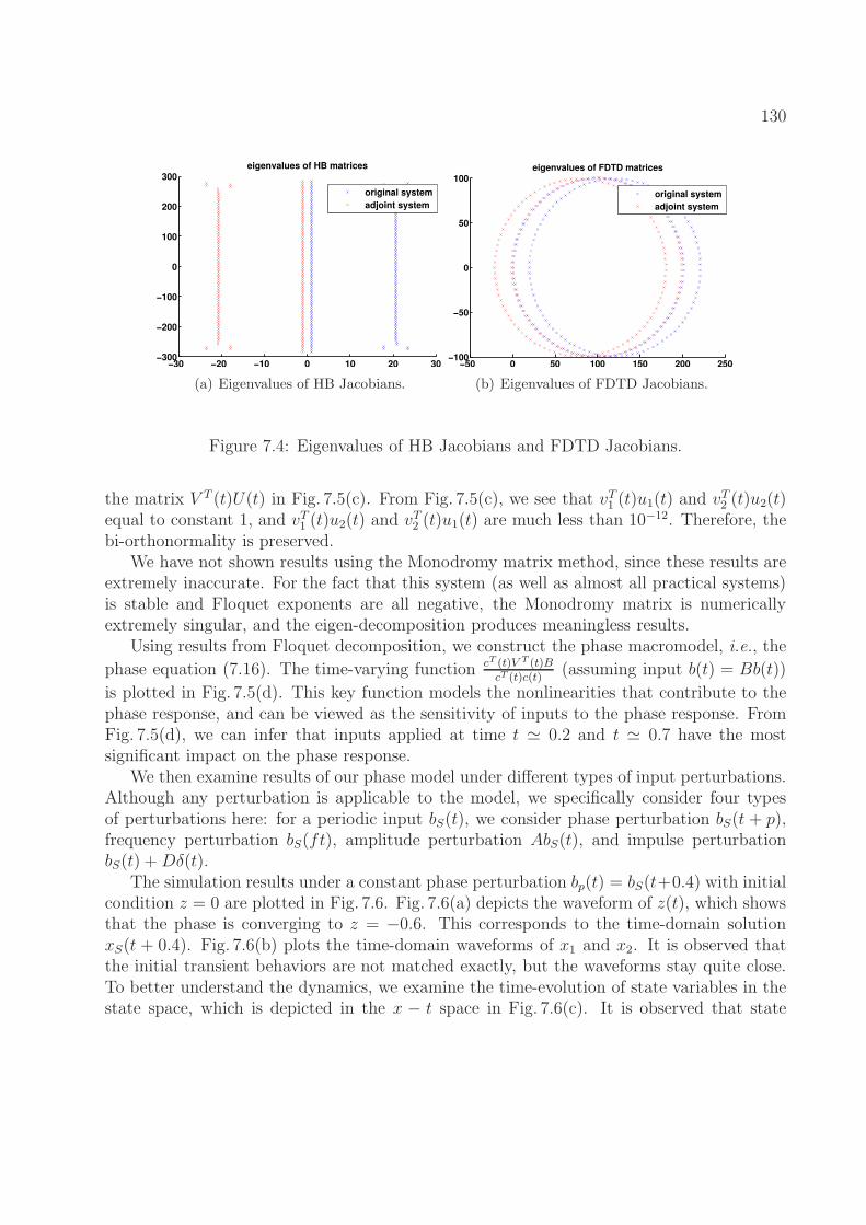
130

−30 −20 −10 0 10 20 30−300

−200

−100

0

100

200

300eigenvalues of HB matrices

original system

adjoint system

(a) Eigenvalues of HB Jacobians.

−50 0 50 100 150 200 250−100

−50

0

50

100eigenvalues of FDTD matrices

original system

adjoint system

(b) Eigenvalues of FDTD Jacobians.

Figure 7.4: Eigenvalues of HB Jacobians and FDTD Jacobians.

the matrix V T (t)U(t) in Fig. 7.5(c). From Fig. 7.5(c), we see that vT1 (t)u1(t) and vT2 (t)u2(t)equal to constant 1, and vT1 (t)u2(t) and vT2 (t)u1(t) are much less than 10−12. Therefore, thebi-orthonormality is preserved.

We have not shown results using the Monodromy matrix method, since these results areextremely inaccurate. For the fact that this system (as well as almost all practical systems)is stable and Floquet exponents are all negative, the Monodromy matrix is numericallyextremely singular, and the eigen-decomposition produces meaningless results.

Using results from Floquet decomposition, we construct the phase macromodel, i.e., the

phase equation (7.16). The time-varying function cT (t)V T (t)BcT (t)c(t)

(assuming input b(t) = Bb(t))

is plotted in Fig. 7.5(d). This key function models the nonlinearities that contribute to thephase response, and can be viewed as the sensitivity of inputs to the phase response. FromFig. 7.5(d), we can infer that inputs applied at time t ≃ 0.2 and t ≃ 0.7 have the mostsignificant impact on the phase response.

We then examine results of our phase model under different types of input perturbations.Although any perturbation is applicable to the model, we specifically consider four typesof perturbations here: for a periodic input bS(t), we consider phase perturbation bS(t + p),frequency perturbation bS(ft), amplitude perturbation AbS(t), and impulse perturbationbS(t) +Dδ(t).

The simulation results under a constant phase perturbation bp(t) = bS(t+0.4) with initialcondition z = 0 are plotted in Fig. 7.6. Fig. 7.6(a) depicts the waveform of z(t), which showsthat the phase is converging to z = −0.6. This corresponds to the time-domain solutionxS(t + 0.4). Fig. 7.6(b) plots the time-domain waveforms of x1 and x2. It is observed thatthe initial transient behaviors are not matched exactly, but the waveforms stay quite close.To better understand the dynamics, we examine the time-evolution of state variables in thestate space, which is depicted in the x − t space in Fig. 7.6(c). It is observed that state

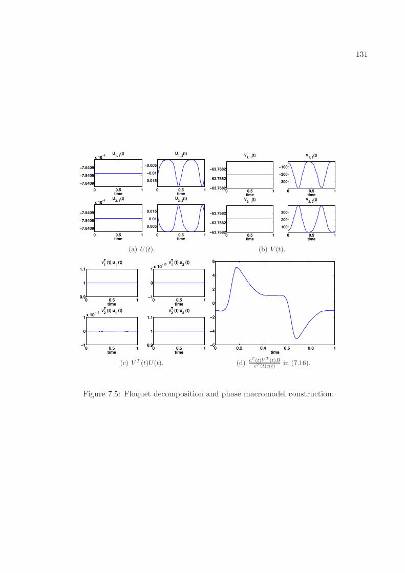
131

0 0.5 1

−7.8409

−7.8409

−7.8409

x 10−3

U1, 1

(t)

time0 0.5 1

−0.015

−0.01

−0.005

U1, 2

(t)

time

0 0.5 1

−7.8409

−7.8409

−7.8409

x 10−3

U2, 1

(t)

time0 0.5 1

0.005

0.01

0.015

U2, 2

(t)

time

(a) U(t).

0 0.5 1−63.7682

−63.7682

−63.7682

V1, 1

(t)

time0 0.5 1

−300

−200

−100

V1, 2

(t)

time

0 0.5 1−63.7682

−63.7682

−63.7682

V2, 1

(t)

time0 0.5 1

100

200

300

V2, 2

(t)

time

(b) V (t).

0 0.5 10.9

1

1.1

v1

T (t) u

1 (t)

time0 0.5 1

−1

0

1x 10

−12v

1

T (t) u

2 (t)

time

0 0.5 1−1

0

1x 10

−12v

2

T (t) u

1 (t)

time0 0.5 1

0.9

1

1.1

v2

T (t) u

2 (t)

time

(c) V T (t)U(t).

0 0.2 0.4 0.6 0.8 1−6

−4

−2

0

2

4

6

time

(d) cT (t)V T (t)BcT (t)c(t) in (7.16).

Figure 7.5: Floquet decomposition and phase macromodel construction.

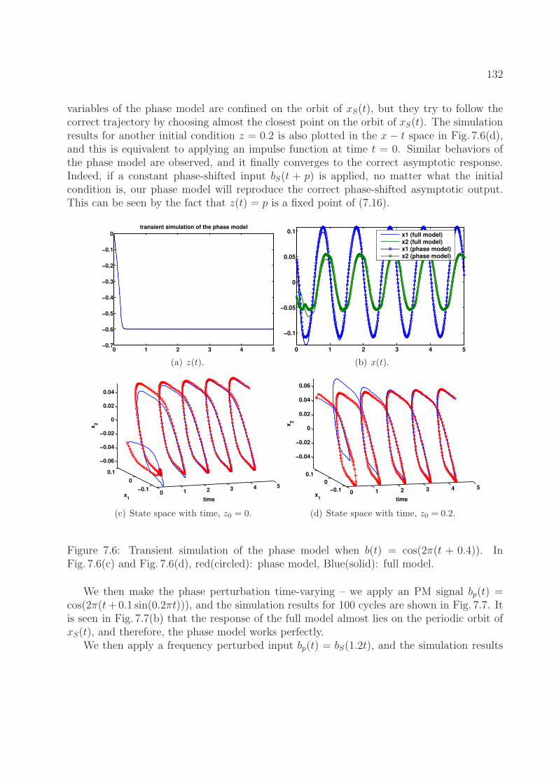
132

variables of the phase model are confined on the orbit of xS(t), but they try to follow thecorrect trajectory by choosing almost the closest point on the orbit of xS(t). The simulationresults for another initial condition z = 0.2 is also plotted in the x − t space in Fig. 7.6(d),and this is equivalent to applying an impulse function at time t = 0. Similar behaviors ofthe phase model are observed, and it finally converges to the correct asymptotic response.Indeed, if a constant phase-shifted input bS(t + p) is applied, no matter what the initialcondition is, our phase model will reproduce the correct phase-shifted asymptotic output.This can be seen by the fact that z(t) = p is a fixed point of (7.16).

0 1 2 3 4 5−0.7

−0.6

−0.5

−0.4

−0.3

−0.2

−0.1

0transient simulation of the phase model

(a) z(t).

0 1 2 3 4 5

−0.1

−0.05

0

0.05

0.1

x1 (full model)x2 (full model)x1 (phase model)x2 (phase model)

(b) x(t).

0 1 2 3 4 5−0.1

0

0.1

−0.06

−0.04

−0.02

0

0.02

0.04

timex

1

x2

(c) State space with time, z0 = 0.

0 1 2 3 4 5−0.1

0

0.1

−0.04

−0.02

0

0.02

0.04

0.06

timex

1

x2

(d) State space with time, z0 = 0.2.

Figure 7.6: Transient simulation of the phase model when b(t) = cos(2π(t + 0.4)). InFig. 7.6(c) and Fig. 7.6(d), red(circled): phase model, Blue(solid): full model.

We then make the phase perturbation time-varying – we apply an PM signal bp(t) =cos(2π(t+0.1 sin(0.2πt))), and the simulation results for 100 cycles are shown in Fig. 7.7. Itis seen in Fig. 7.7(b) that the response of the full model almost lies on the periodic orbit ofxS(t), and therefore, the phase model works perfectly.

We then apply a frequency perturbed input bp(t) = bS(1.2t), and the simulation results

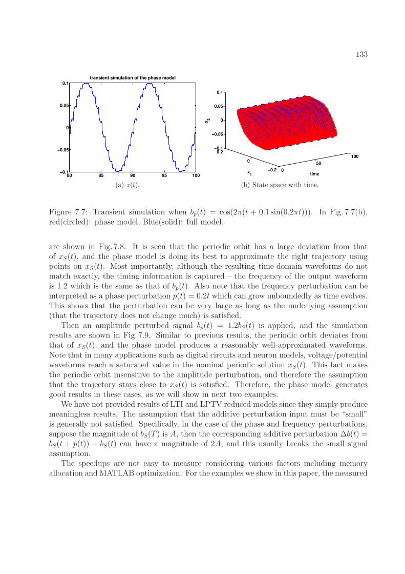
133

80 85 90 95 100−0.1

−0.05

0

0.05

0.1transient simulation of the phase model

(a) z(t).

0

50

100

−0.2

0

0.2−0.1

−0.05

0

0.05

0.1

timex1

x2

(b) State space with time.

Figure 7.7: Transient simulation when bp(t) = cos(2π(t + 0.1 sin(0.2πt))). In Fig. 7.7(b),red(circled): phase model, Blue(solid): full model.

are shown in Fig. 7.8. It is seen that the periodic orbit has a large deviation from thatof xS(t), and the phase model is doing its best to approximate the right trajectory usingpoints on xS(t). Most importantly, although the resulting time-domain waveforms do notmatch exactly, the timing information is captured – the frequency of the output waveformis 1.2 which is the same as that of bp(t). Also note that the frequency perturbation can beinterpreted as a phase perturbation p(t) = 0.2t which can grow unboundedly as time evolves.This shows that the perturbation can be very large as long as the underlying assumption(that the trajectory does not change much) is satisfied.

Then an amplitude perturbed signal bp(t) = 1.2bS(t) is applied, and the simulationresults are shown in Fig. 7.9. Similar to previous results, the periodic orbit deviates fromthat of xS(t), and the phase model produces a reasonably well-approximated waveforms.Note that in many applications such as digital circuits and neuron models, voltage/potentialwaveforms reach a saturated value in the nominal periodic solution xS(t). This fact makesthe periodic orbit insensitive to the amplitude perturbation, and therefore the assumptionthat the trajectory stays close to xS(t) is satisfied. Therefore, the phase model generatesgood results in these cases, as we will show in next two examples.

We have not provided results of LTI and LPTV reduced models since they simply producemeaningless results. The assumption that the additive perturbation input must be “small”is generally not satisfied. Specifically, in the case of the phase and frequency perturbations,suppose the magnitude of bS(T ) is A, then the corresponding additive perturbation ∆b(t) =bS(t + p(t)) − bS(t) can have a magnitude of 2A, and this usually breaks the small signalassumption.

The speedups are not easy to measure considering various factors including memoryallocation and MATLAB optimization. For the examples we show in this paper, the measured

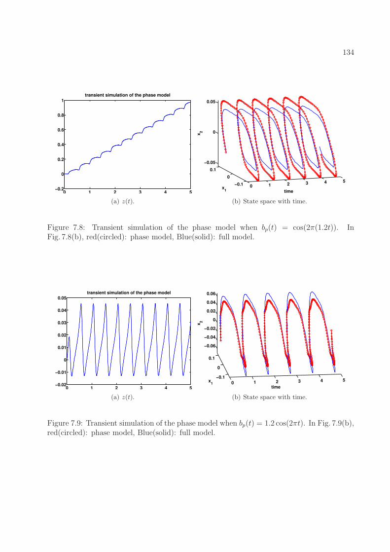
134

0 1 2 3 4 5−0.2

0

0.2

0.4

0.6

0.8


(a) z(t).

0 1 2 3 4 5−0.1

0

0.1

−0.05

0

0.05

timex

1

x2


Figure 7.8: Transient simulation of the phase model when bp(t) = cos(2π(1.2t)). InFig. 7.8(b), red(circled): phase model, Blue(solid): full model.

0 1 2 3 4 5−0.02

−0.01

0

0.01

0.02

0.03

0.04


(a) z(t).

0 1 2 3 4 5−0.1

0

0.1

−0.06

−0.04

−0.02

0

0.02

0.04

0.06

time

x1

x2


Figure 7.9: Transient simulation of the phase model when bp(t) = 1.2 cos(2πt). In Fig. 7.9(b),red(circled): phase model, Blue(solid): full model.

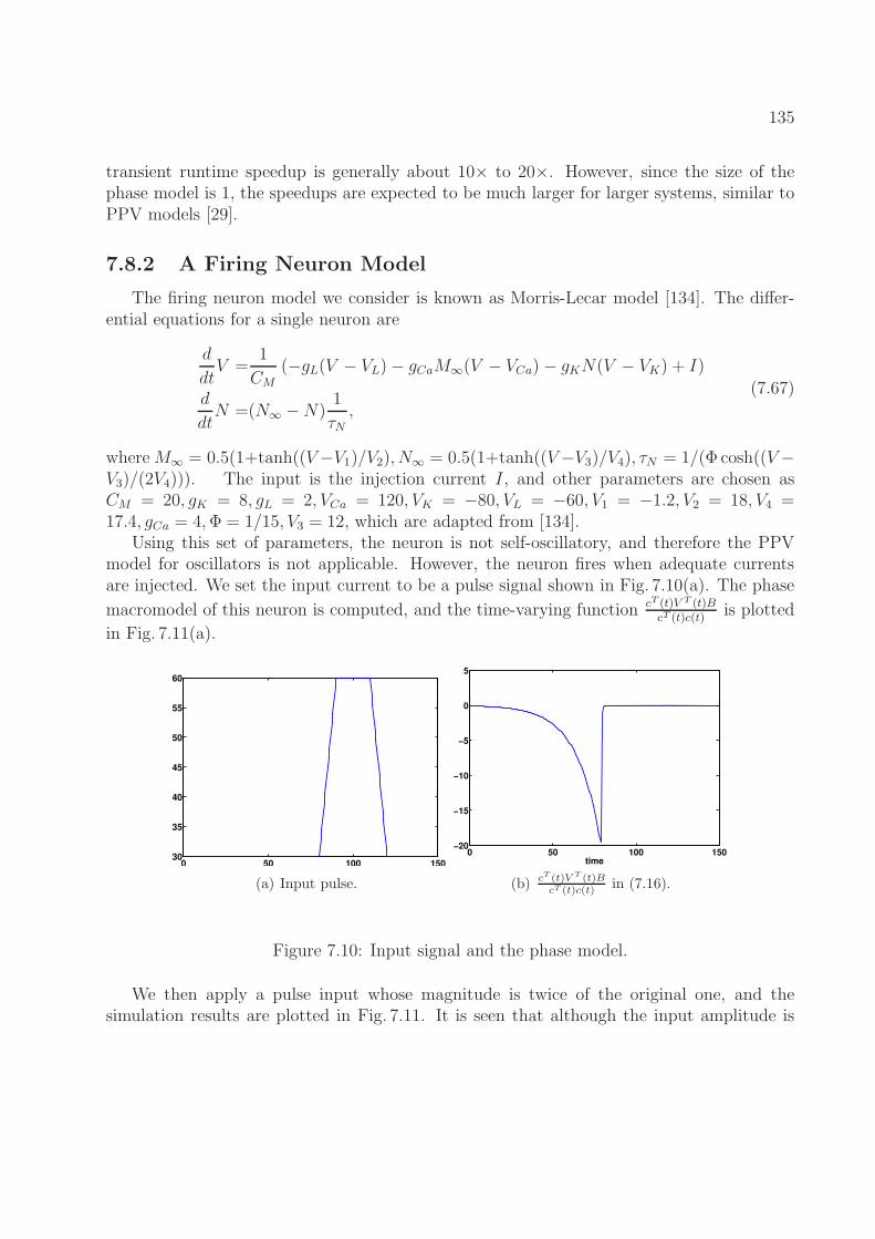
135

transient runtime speedup is generally about 10× to 20×. However, since the size of thephase model is 1, the speedups are expected to be much larger for larger systems, similar toPPV models [29].

7.8.2 A Firing Neuron Model

The firing neuron model we consider is known as Morris-Lecar model [134]. The differ-ential equations for a single neuron are

d

dtV =

1

CM

(−gL(V − VL)− gCaM∞(V − VCa)− gKN(V − VK) + I)

d

dtN =(N∞ −N)

1

τN,

(7.67)

whereM∞ = 0.5(1+tanh((V−V1)/V2), N∞ = 0.5(1+tanh((V−V3)/V4), τN = 1/(Φ cosh((V−V3)/(2V4))). The input is the injection current I, and other parameters are chosen asCM = 20, gK = 8, gL = 2, VCa = 120, VK = −80, VL = −60, V1 = −1.2, V2 = 18, V4 =17.4, gCa = 4,Φ = 1/15, V3 = 12, which are adapted from [134].

Using this set of parameters, the neuron is not self-oscillatory, and therefore the PPVmodel for oscillators is not applicable. However, the neuron fires when adequate currentsare injected. We set the input current to be a pulse signal shown in Fig. 7.10(a). The phase

macromodel of this neuron is computed, and the time-varying function cT (t)V T (t)BcT (t)c(t)

is plotted

in Fig. 7.11(a).

0 50 100 15030

35

40

45

50

55

60

(a) Input pulse.

0 50 100 150−20

−15

−10

−5

0

5

time

(b) cT (t)V T (t)BcT (t)c(t) in (7.16).

Figure 7.10: Input signal and the phase model.

We then apply a pulse input whose magnitude is twice of the original one, and thesimulation results are plotted in Fig. 7.11. It is seen that although the input amplitude is

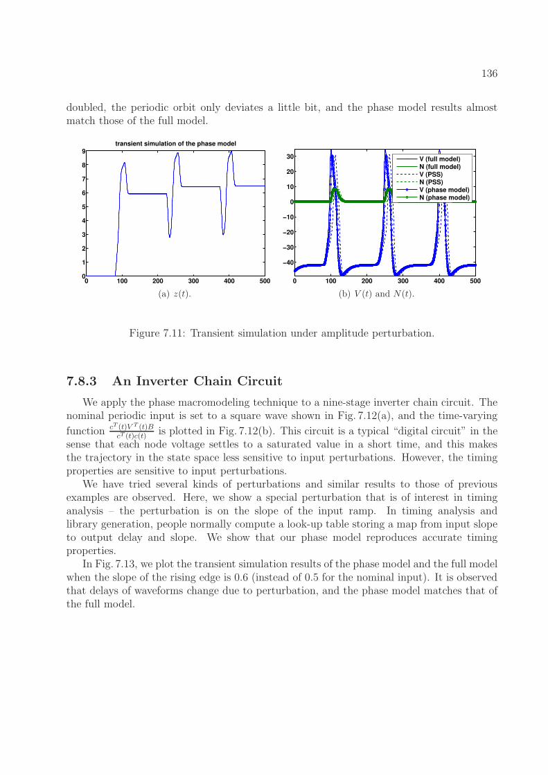
136

doubled, the periodic orbit only deviates a little bit, and the phase model results almostmatch those of the full model.

0 100 200 300 400 5000

1

2

3

4

5

6

7

8


(a) z(t).

0 100 200 300 400 500

−40

−30

−20

−10

0

10

20

30

V (full model)N (full model)V (PSS)N (PSS)V (phase model)N (phase model)

(b) V (t) and N(t).

Figure 7.11: Transient simulation under amplitude perturbation.

7.8.3 An Inverter Chain Circuit

We apply the phase macromodeling technique to a nine-stage inverter chain circuit. Thenominal periodic input is set to a square wave shown in Fig. 7.12(a), and the time-varying

function cT (t)V T (t)BcT (t)c(t)

is plotted in Fig. 7.12(b). This circuit is a typical “digital circuit” in thesense that each node voltage settles to a saturated value in a short time, and this makesthe trajectory in the state space less sensitive to input perturbations. However, the timingproperties are sensitive to input perturbations.

We have tried several kinds of perturbations and similar results to those of previousexamples are observed. Here, we show a special perturbation that is of interest in timinganalysis – the perturbation is on the slope of the input ramp. In timing analysis andlibrary generation, people normally compute a look-up table storing a map from input slopeto output delay and slope. We show that our phase model reproduces accurate timingproperties.

In Fig. 7.13, we plot the transient simulation results of the phase model and the full modelwhen the slope of the rising edge is 0.6 (instead of 0.5 for the nominal input). It is observedthat delays of waveforms change due to perturbation, and the phase model matches that ofthe full model.

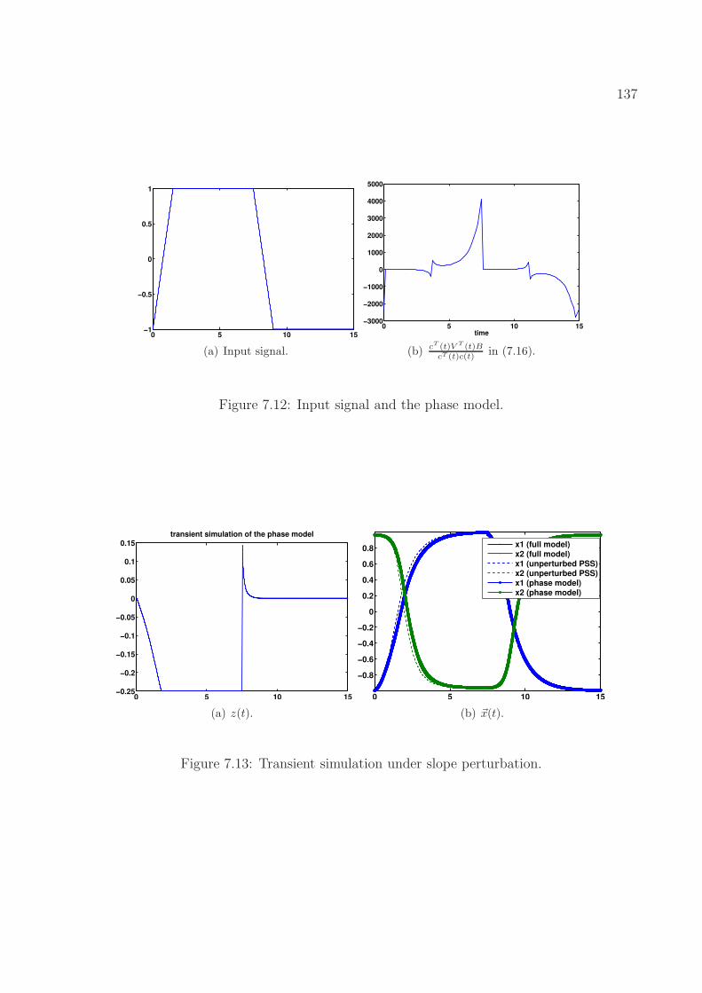
137

0 5 10 15−1

−0.5

0

0.5

1

(a) Input signal.

0 5 10 15−3000

−2000

−1000

0

1000

2000

3000

4000

5000

time

(b) cT (t)V T (t)BcT (t)c(t) in (7.16).

Figure 7.12: Input signal and the phase model.

0 5 10 15−0.25

−0.2

−0.15

−0.1

−0.05

0

0.05

0.1


(a) z(t).

0 5 10 15

−0.8

−0.6

−0.4

−0.2

0

0.2

0.4

0.6

0.8

x1 (full model)x2 (full model)x1 (unperturbed PSS)x2 (unperturbed PSS)x1 (phase model)x2 (phase model)

(b) ~x(t).

Figure 7.13: Transient simulation under slope perturbation.

138

Chapter 8

DAE2FSM: Finite State MachineAbstraction from DifferentialEquations

In this chapter, we study a different problem in which a finite state machine, insteadof a smaller set of differential equations, is abstracted from original differential equations.The problem is motivated by the fact that in modern digital designs, circuit behaviors maynot be accurately modeled by the ideal pre-specified finite state machines, due to parametervariations, crosstalk and coupling, environment changes, etc.. As a result, a ground-upabstraction of the finite state machine from differential equations, deemed as the goldenmodel, is needed. Other than the circuit applications, the model is also found useful in otherengineering problems, such as biological systems.

We start with a detailed comparison of DAE/ODE models and FSM models that shedlight on the validity of such abstractions and the approach we may follow. Then we re-view several existing approaches in the community of machine learning1, and discuss howwe adapt these algorithms in learning differential equations. The key challenge is to developcorresponding concepts/subroutines in those of machine learning, such as state merging andequivalence checking. We present experimental results of several systems, and show appli-cations of the finite state machines learned in further system-level simulation and analysis.

8.1 Problem Formulation

The problem of FSM abstraction is one variation of the problem (2.1) in Section 2.1,whereM is the set of ODEs/DAEs, andMr is the set of finite state machines. The funda-mental questions are similar, i.e.,

1The term machine learning here refers to the actual finite state machine learning, rather than statisticallearning such as learning Bayesian networks.

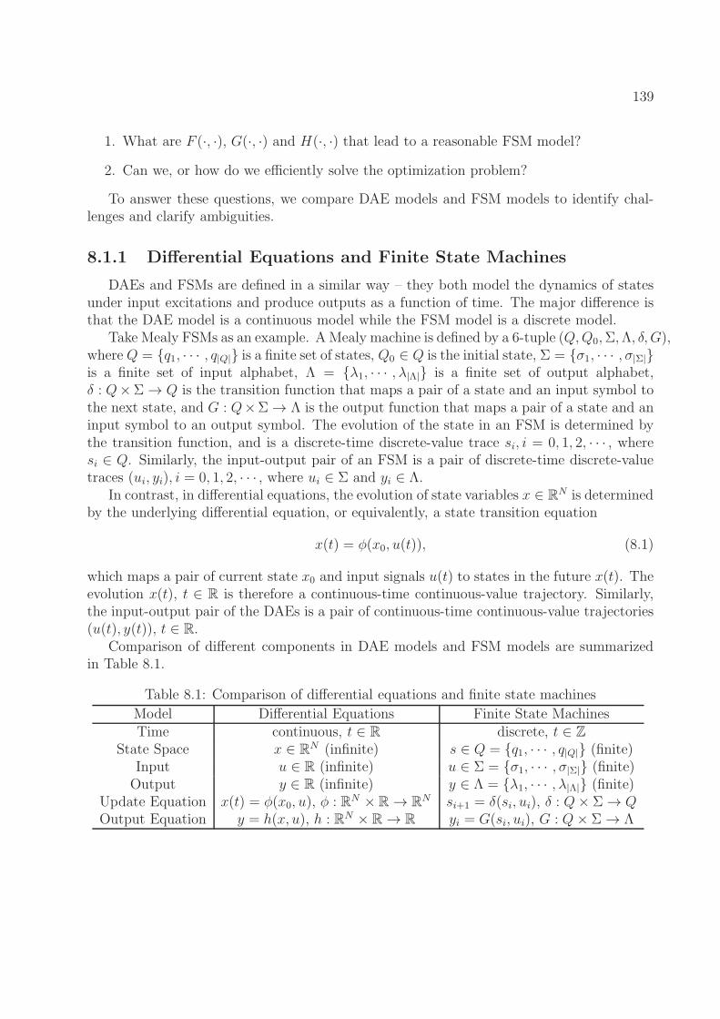
139

1. What are F (·, ·), G(·, ·) and H(·, ·) that lead to a reasonable FSM model?

2. Can we, or how do we efficiently solve the optimization problem?

To answer these questions, we compare DAE models and FSM models to identify chal-lenges and clarify ambiguities.

8.1.1 Differential Equations and Finite State Machines

DAEs and FSMs are defined in a similar way – they both model the dynamics of statesunder input excitations and produce outputs as a function of time. The major difference isthat the DAE model is a continuous model while the FSM model is a discrete model.

Take Mealy FSMs as an example. A Mealy machine is defined by a 6-tuple (Q,Q0,Σ,Λ, δ, G),where Q = q1, · · · , q|Q| is a finite set of states, Q0 ∈ Q is the initial state, Σ = σ1, · · · , σ|Σ|is a finite set of input alphabet, Λ = λ1, · · · , λ|Λ| is a finite set of output alphabet,δ : Q×Σ→ Q is the transition function that maps a pair of a state and an input symbol tothe next state, and G : Q×Σ→ Λ is the output function that maps a pair of a state and aninput symbol to an output symbol. The evolution of the state in an FSM is determined bythe transition function, and is a discrete-time discrete-value trace si, i = 0, 1, 2, · · · , wheresi ∈ Q. Similarly, the input-output pair of an FSM is a pair of discrete-time discrete-valuetraces (ui, yi), i = 0, 1, 2, · · · , where ui ∈ Σ and yi ∈ Λ.

In contrast, in differential equations, the evolution of state variables x ∈ RN is determined

by the underlying differential equation, or equivalently, a state transition equation

x(t) = φ(x0, u(t)), (8.1)

which maps a pair of current state x0 and input signals u(t) to states in the future x(t). Theevolution x(t), t ∈ R is therefore a continuous-time continuous-value trajectory. Similarly,the input-output pair of the DAEs is a pair of continuous-time continuous-value trajectories(u(t), y(t)), t ∈ R.

Comparison of different components in DAE models and FSM models are summarizedin Table 8.1.

Table 8.1: Comparison of differential equations and finite state machines

Model Differential Equations Finite State MachinesTime continuous, t ∈ R discrete, t ∈ Z

State Space x ∈ RN (infinite) s ∈ Q = q1, · · · , q|Q| (finite)

Input u ∈ R (infinite) u ∈ Σ = σ1, · · · , σ|Σ| (finite)Output y ∈ R (infinite) y ∈ Λ = λ1, · · · , λ|Λ| (finite)

Update Equation x(t) = φ(x0, u), φ : RN × R→ RN si+1 = δ(si, ui), δ : Q× Σ→ Q

Output Equation y = h(x, u), h : RN × R→ R yi = G(si, ui), G : Q× Σ→ Λ

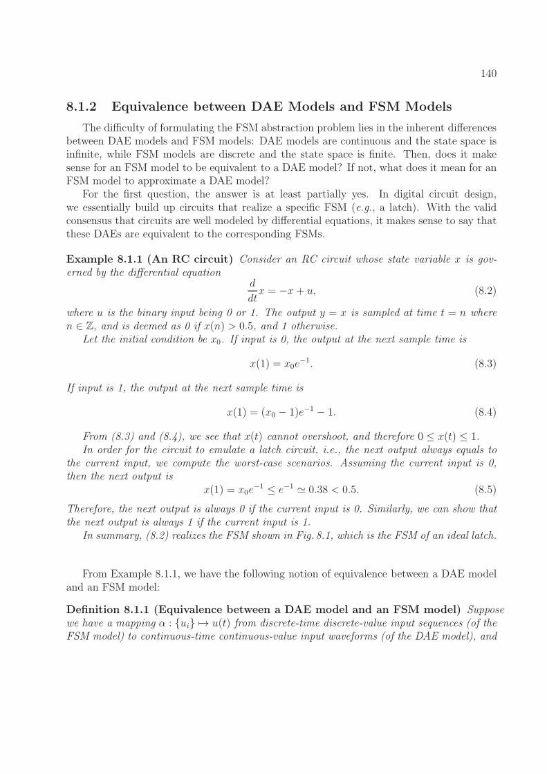
140

8.1.2 Equivalence between DAE Models and FSM Models

The difficulty of formulating the FSM abstraction problem lies in the inherent differencesbetween DAE models and FSM models: DAE models are continuous and the state space isinfinite, while FSM models are discrete and the state space is finite. Then, does it makesense for an FSM model to be equivalent to a DAE model? If not, what does it mean for anFSM model to approximate a DAE model?

For the first question, the answer is at least partially yes. In digital circuit design,we essentially build up circuits that realize a specific FSM (e.g., a latch). With the validconsensus that circuits are well modeled by differential equations, it makes sense to say thatthese DAEs are equivalent to the corresponding FSMs.

Example 8.1.1 (An RC circuit) Consider an RC circuit whose state variable x is gov-erned by the differential equation

d

dtx = −x+ u, (8.2)

where u is the binary input being 0 or 1. The output y = x is sampled at time t = n wheren ∈ Z, and is deemed as 0 if x(n) > 0.5, and 1 otherwise.

Let the initial condition be x0. If input is 0, the output at the next sample time is

x(1) = x0e−1. (8.3)

If input is 1, the output at the next sample time is

x(1) = (x0 − 1)e−1 − 1. (8.4)

From (8.3) and (8.4), we see that x(t) cannot overshoot, and therefore 0 ≤ x(t) ≤ 1.In order for the circuit to emulate a latch circuit, i.e., the next output always equals to

the current input, we compute the worst-case scenarios. Assuming the current input is 0,then the next output is

x(1) = x0e−1 ≤ e−1 ≃ 0.38 < 0.5. (8.5)

Therefore, the next output is always 0 if the current input is 0. Similarly, we can show thatthe next output is always 1 if the current input is 1.

In summary, (8.2) realizes the FSM shown in Fig. 8.1, which is the FSM of an ideal latch.

From Example 8.1.1, we have the following notion of equivalence between a DAE modeland an FSM model:

Definition 8.1.1 (Equivalence between a DAE model and an FSM model) Supposewe have a mapping α : ui 7→ u(t) from discrete-time discrete-value input sequences (of theFSM model) to continuous-time continuous-value input waveforms (of the DAE model), and

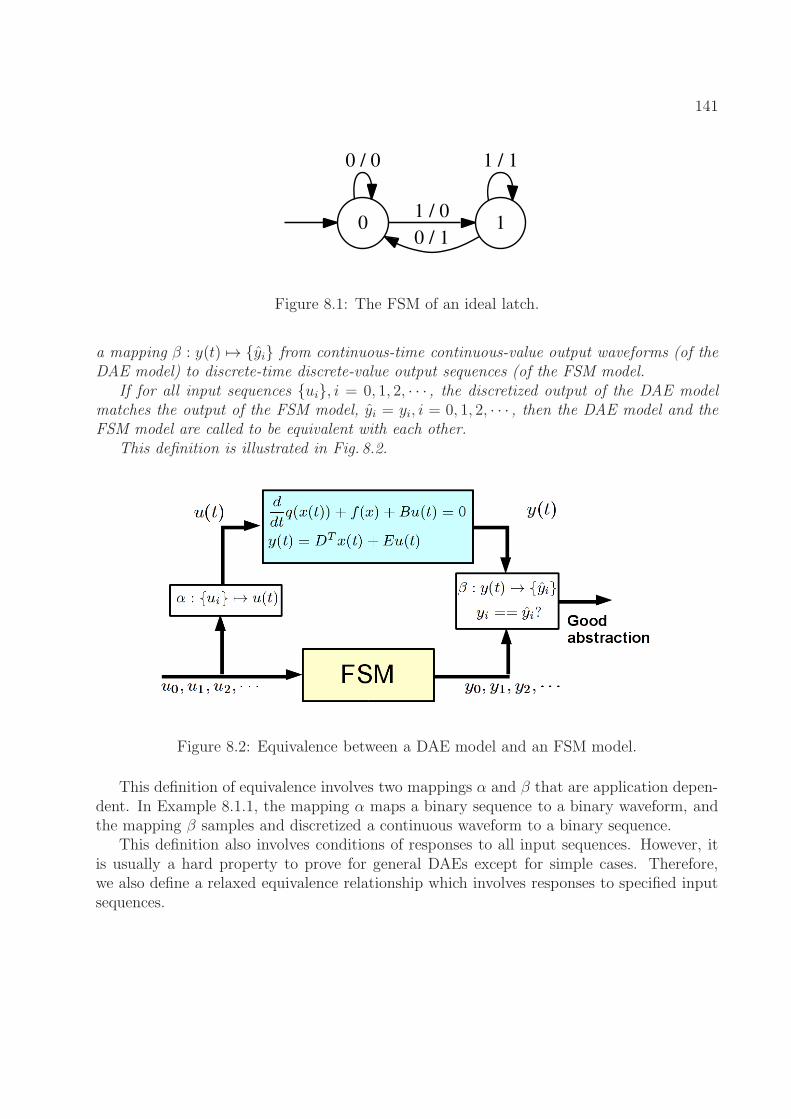
141

0

0 / 0

11 / 0

0 / 1

1 / 1

Figure 8.1: The FSM of an ideal latch.

a mapping β : y(t) 7→ yi from continuous-time continuous-value output waveforms (of theDAE model) to discrete-time discrete-value output sequences (of the FSM model.

If for all input sequences ui, i = 0, 1, 2, · · · , the discretized output of the DAE modelmatches the output of the FSM model, yi = yi, i = 0, 1, 2, · · · , then the DAE model and theFSM model are called to be equivalent with each other.

This definition is illustrated in Fig. 8.2.

Figure 8.2: Equivalence between a DAE model and an FSM model.

This definition of equivalence involves two mappings α and β that are application depen-dent. In Example 8.1.1, the mapping α maps a binary sequence to a binary waveform, andthe mapping β samples and discretized a continuous waveform to a binary sequence.

This definition also involves conditions of responses to all input sequences. However, itis usually a hard property to prove for general DAEs except for simple cases. Therefore,we also define a relaxed equivalence relationship which involves responses to specified inputsequences.

142

Definition 8.1.2 (U-Equivalence between a DAE model and an FSM model) Supposewe have a mapping α : ui 7→ u(t) from discrete-time discrete-value input sequences (of theFSM model) to continuous-time continuous-value input waveforms (of the DAE model), anda mapping β : y(t) 7→ yi from continuous-time continuous-value output waveforms (of theDAE model) to discrete-time discrete-value output sequences (of the FSM model.

If for all input sequences ui ∈ U which is a subset of input sequences, the discretizedoutput of the DAE model matches the output of the FSM model, yi = yi, i = 0, 1, 2, · · · , thenthe DAE model and the FSM model are called to be U-equivalent with each other.

For example, U can be the set of input sequences of fixed length L. This is indeedreasonable in many practical applications because system state evolves from a steady statefor some time and gets reset once in a while. For example, in a communication system or ahigh-speed link, the circuits are reset after each packet is transmitted/received. Therefore,the models will be good enough if they matches the responses to input sequences of lengthequal to the packet size.

This relaxed definition therefore specifies an FSM approximation to the original DAEmodel. By specifying different U ’s in different applications, we obtain different levels ofapproximations.

Another notion of equivalence may be defined by discretizing the continuous state spaceof the DAE model and adding transitions among different regions. Denote X(si) to be theregion in R

N corresponding to the state si. The transition from one state si to another state sjis added if there exists a point xi ∈ X(si) and an input ui ∈ Σ such that φ(xi, α(ui)) ∈ X(sj).For example, in Fig. 8.2, the state 0 corresponds to the half space x < 0.5 and the state 1corresponds to the half space x ≥ 0.5. and the transitions are added by the rule above.

While this conversion from a DAE model to an FSM model seems to be straightforwardfor the above simple example, it is not generally the case. Consider a similar example asExample 8.1.1, where the dynamics of x is defined by

d

dtx = −0.5x+ u. (8.6)

In this case, if we still use the same partitioning, then we may have an FSM with more than4 transitions, leading to a non-deterministic FSM. Also, in general, it may not be possible toexamine every point in a region, and some transitions may be lost. While a non-deterministicFSM may be useful, it may be useless if there are too many transitions that little informationof the DAE behaviors is modeled.

143

8.1.3 FSM Abstraction Formulation

Based on the above definition, we can formulate a simplistic FSM abstraction problemin the form of (2.1):

minimizeFSMs

1

subject to The FSM model is U-equivalent to the DAE model(8.7)

where we set F (·, ·) to be constant 1, H(·, ·) to be empty, and G(·, ·) is the difference betweenthe discretized outputs of the DAE model and the outputs of the FSM model.

In another word, in problem (8.7), we are given a set of input-output trajectories of aDAE model, and we try to find an FSM model that matches these input-output trajectories.It appears that there have been efficient algorithms developed in other areas such as soft-ware verification and machine learning that solves similar problems. We will study some ofthem in the following sections, and develop sufficient adaptations and modifications of thesealgorithms to solve our problem.

The optimization problem (8.7), however, does not have a unique solution. To ensure aunique solution, we may formulate more sophisticated problems by adding/choosing otherF,G,H functions. For example, we may minimize the number of states of the FSM model,or enforcing deterministicity of the FSM model, by modifying F and H respectively.

8.2 Review of FSM Abstraction Methods

8.2.1 Angluin’s DFA Learning Algorithm

ADFA (Deterministic Finite Automaton) is a machine consisting of a 5-tuple: (Q,Σ, δ, Q0, F ),where Q is a finite set of states, Σ is a finite set of input alphabet, δ : Q × Σ → Q is thetransition function, Q0 is the start state, F ⊂ Q is a set of accept states. Under the inputsequence w, if the final state is in the set of accept states, the machine is said to accept w.Otherwise, it rejects w.

Given a DFA, Angluin’s algorithm aims to learn the exact DFA from I/O traces of theDFA. The basic idea is to repeatedly conjecture machines according to I/O traces until anequivalent machine is obtained. The key data structure of the algorithm is an observa-tion table which keeps track of necessary simulation results from which a machine can beconjectured.

An example of the observation table T is shown Table 8.2, where λ means “empty”, theset of row labels is called S and the set of column labels is called E, according to Angluin’snotation. To fill in each cell of the table, we concatenate the row label with the column label,use that as the input sequence to the DFA to perform a membership query (simulation), andfill in the yes/no answer (to whether the DFA accepts this input sequence) in the cell. The

144

observation table is further split into the top part and the bottom part, where row labelsof the bottom part are obtained by concatenating row labels of the top part with all inputalphabets. We will regard each row in the top part of the table as one state in the statemachine, and therefore for each state in the top table, there must exist a row in the tablethat corresponds to its next state.

With the observation table, the key idea is then to differentiate different states by exper-iments, i.e., we regard two rows as the same state if entries of the two rows are the same.For example, row “1” has the same entries as row “110” in Table 8.2, and therefore representthe same state. However, to conjecture a DFA from an observation table, we need to placetwo constraints on the table:

1. The table is closed, i.e., every row in the bottom part of the table has a correspondingrow in the top part with identical results in all columns. This guarantees that none ofthe rows in the bottom part corresponds to a new state.

2. The table is consistent, i.e., every pair of rows in the top part of the table with identicalresults in all columns also has identical results when any alphabet symbol is added.Mathematically, ∀s1, s2 ∈ S, if row(s1) = row(s2), then ∀a ∈ Σ, row(s1 ·a) = row(s2 ·a).This guarantees that any pair of states that we think are the same are still the sameif the experiment string is extended by one input alphabet symbol.

The procedures to make the observation table closed and consistent are simple, and can befound in [135].

Given a closed and consistent observation table (S,E, T ), we can then conjecture a DFA(Q,Σ, δ, Q0, F ) defined by

Q = row(s) : s ∈ S of top table,Q0 = row(λ),

δ(row(s), a) = row(s · a), a ∈ Σ,

F = row(s) : T (s, λ) = 1.

(8.8)

Using this DFA, we can feed it to an “equivalence checker” to check if the DFA is equiv-alent to the original one. If equivalence checker returns “yes”, we terminate the algorithm.Otherwise, it returns an counter-example. In that case, we add the counter-example into theobservation table, and repeat the procedure of conjecturing a new DFA until convergence.

Summarizing the above procedure, the Angluin’s algorithm is sketched in Algorithm 13.

8.2.2 Extension to Learning Mealy Machines

As defined in Section 8.1.1, the Mealy machine is similar to a DFA. It does not haveaccept states in DFA, but has an output function. This difference requires us to re-define

145

Algorithm 13 Angluin’s DFA learning algorithm

1: Construct the initial observation table (S,E, T ) with S = λ and E = λ.2: repeat3: Make the observation table (S,E, T ) closed and consistent.4: Conjecture a DFA according to (8.8).5: Check the equivalence between the conjectured DFA and the original DFA.6: if not equivalent then7: Add the counter-example in the observation table.8: end if9: until Equivalence checker returns “yes”.

the meaning of the observation table.In Angluin’s algorithm, each cell in the table is filled in by yes/no answers to whether the

DFA accepts an input sequence. This can be viewed as the “output” of the DFA. Similarly,for Mealy machines, we can fill in each cell in the table by the output of the Mealy machine.It turns out that using this new definition of the observation table, the concepts of closed-ness and consistence of the observation table still holds [136], and we can conjecture a Mealymachine (Q,Q0,Σ,Λ, δ, G) from this new observation table by

Q = row(s) : s ∈ S of top table,Q0 = row(λ),

δ(row(s), a) = row(s · a), a ∈ Σ,

G(row(s), a) = T (s, a), a ∈ Σ.

(8.9)

Therefore, in order to learn a Mealy machine from another Mealy machine using Angluin’sidea, we just need to use the new observation table, and replace step 4 in Algorithm 13 by“Conjecture a Mealy machine according to (8.9)”.

8.3 Adaptation of Angluin’s Algorithm

In this section, we describe adaptations of Angluin’s algorithm to learn Mealy machinesfrom differential equations. We show how we implement two key subroutines that are re-peatedly called by Angluin’s algorithm, and we interpret the states in the resulting Mealymachine in terms of regions in the original continuous state space. This connection also leadsto a partitioning of the continuous state space.

In Angluin’s algorithm, there are two subroutines that are repeatedly called:

1. The simulator. When building the observation table, the table entries are obtainedby making membership queries (i.e., is w accepted by the DFA?). In the case oflearning Mealy machines, this corresponds to a simulation of the Mealy machine to

146

obtain the output. Therefore, we need a simulator that can produce I/O traces of amachine/system.

2. The equivalence checker. The algorithm decides whether to terminate by makingequivalence queries (i.e., is the new machine M equivalent to the original machine?).

8.3.1 Implementation of the Simulator

The simulation of circuit differential equations is straightforwardly implemented by SPICEtransient analysis (numerical integration of the differential equations). However, three prob-lems remain to initiate the simulation and interpret the results:

1. To start the simulation, we need to specify an initial condition that corresponds to theinitial state of the Mealy machine;

2. We need to transform the input sequence ui (to the FSM) to the input waveformu(t) (to differential equations).

3. After the simulation, we need to translate the continuous output waveforms to discreteoutputs of the FSM.

To determine the initial condition, we propose to use the DC solution of the circuit. Thisis usually an important state for circuits since circuits typically settle down to this statewhen the input is fixed (except for special cases like oscillators).

The transformation from the input sequence ui to the input waveform u(t) and thetransformation from the output waveform y(t) to output sequences yi are implemented bystandard interpolation and quantization. However, one can define arbitrary transformationsaccording to different applications. For example, the input sequence can specify phases ofthe input waveform at different time points, in which case the input waveforms are obtainedby a transformation from the phase-domain to the voltage-domain. We can also specifybinary values in the input sequence to be corresponding voltage levels of a digital squarewaveform during each clock cycle.

8.3.2 Implementation of the Equivalence Checker

To implement the equivalence checker, we use the U-equivalence defined in Section 8.1.2.Therefore, we call the SPICE simulator to perform a set of simulations of circuit differentialequations using u(t) derived from ui ∈ U . If the sampled outputs y(ih) lie in the cor-responding quantization regions defined for yi (the output of the FSM to input sequenceui), then we return “yes”, i.e., the FSM is equivalent to the differential equations. Other-wise, the input sequence is reported as an counter-example, and is added into the observationtable to refine the FSM.

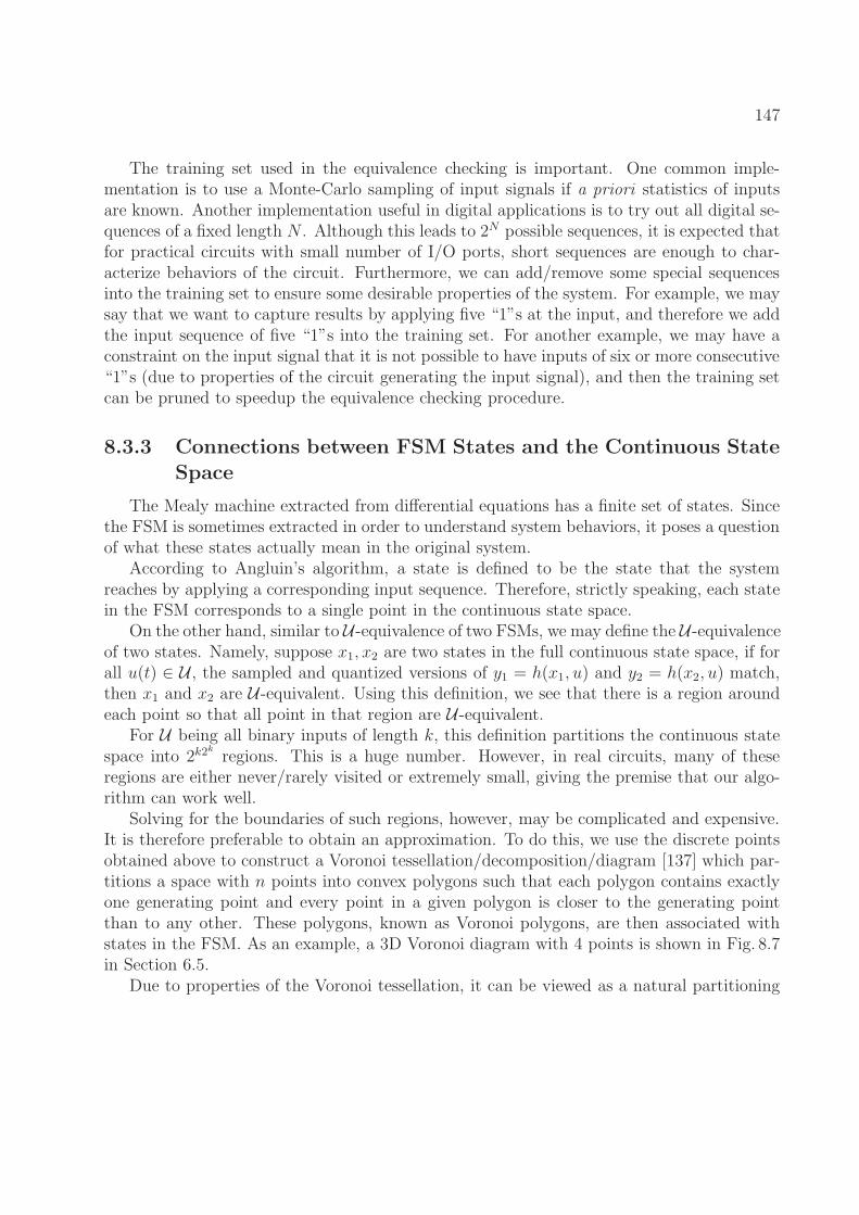
147

The training set used in the equivalence checking is important. One common imple-mentation is to use a Monte-Carlo sampling of input signals if a priori statistics of inputsare known. Another implementation useful in digital applications is to try out all digital se-quences of a fixed length N . Although this leads to 2N possible sequences, it is expected thatfor practical circuits with small number of I/O ports, short sequences are enough to char-acterize behaviors of the circuit. Furthermore, we can add/remove some special sequencesinto the training set to ensure some desirable properties of the system. For example, we maysay that we want to capture results by applying five “1”s at the input, and therefore we addthe input sequence of five “1”s into the training set. For another example, we may have aconstraint on the input signal that it is not possible to have inputs of six or more consecutive“1”s (due to properties of the circuit generating the input signal), and then the training setcan be pruned to speedup the equivalence checking procedure.

8.3.3 Connections between FSM States and the Continuous StateSpace

The Mealy machine extracted from differential equations has a finite set of states. Sincethe FSM is sometimes extracted in order to understand system behaviors, it poses a questionof what these states actually mean in the original system.

According to Angluin’s algorithm, a state is defined to be the state that the systemreaches by applying a corresponding input sequence. Therefore, strictly speaking, each statein the FSM corresponds to a single point in the continuous state space.

On the other hand, similar to U-equivalence of two FSMs, we may define the U-equivalenceof two states. Namely, suppose x1, x2 are two states in the full continuous state space, if forall u(t) ∈ U , the sampled and quantized versions of y1 = h(x1, u) and y2 = h(x2, u) match,then x1 and x2 are U-equivalent. Using this definition, we see that there is a region aroundeach point so that all point in that region are U-equivalent.

For U being all binary inputs of length k, this definition partitions the continuous statespace into 2k2

k

regions. This is a huge number. However, in real circuits, many of theseregions are either never/rarely visited or extremely small, giving the premise that our algo-rithm can work well.

Solving for the boundaries of such regions, however, may be complicated and expensive.It is therefore preferable to obtain an approximation. To do this, we use the discrete pointsobtained above to construct a Voronoi tessellation/decomposition/diagram [137] which par-titions a space with n points into convex polygons such that each polygon contains exactlyone generating point and every point in a given polygon is closer to the generating pointthan to any other. These polygons, known as Voronoi polygons, are then associated withstates in the FSM. As an example, a 3D Voronoi diagram with 4 points is shown in Fig. 8.7in Section 6.5.

Due to properties of the Voronoi tessellation, it can be viewed as a natural partitioning

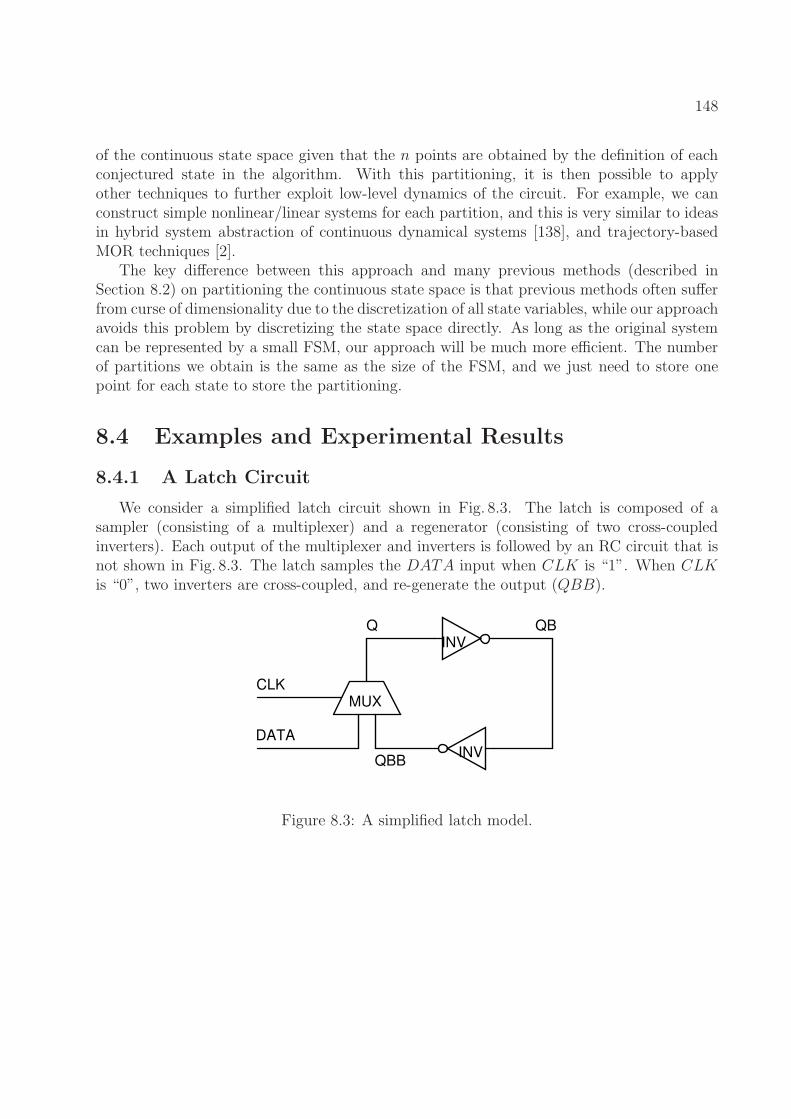
148

of the continuous state space given that the n points are obtained by the definition of eachconjectured state in the algorithm. With this partitioning, it is then possible to applyother techniques to further exploit low-level dynamics of the circuit. For example, we canconstruct simple nonlinear/linear systems for each partition, and this is very similar to ideasin hybrid system abstraction of continuous dynamical systems [138], and trajectory-basedMOR techniques [2].

The key difference between this approach and many previous methods (described inSection 8.2) on partitioning the continuous state space is that previous methods often sufferfrom curse of dimensionality due to the discretization of all state variables, while our approachavoids this problem by discretizing the state space directly. As long as the original systemcan be represented by a small FSM, our approach will be much more efficient. The numberof partitions we obtain is the same as the size of the FSM, and we just need to store onepoint for each state to store the partitioning.


8.4.1 A Latch Circuit

We consider a simplified latch circuit shown in Fig. 8.3. The latch is composed of asampler (consisting of a multiplexer) and a regenerator (consisting of two cross-coupledinverters). Each output of the multiplexer and inverters is followed by an RC circuit that isnot shown in Fig. 8.3. The latch samples the DATA input when CLK is “1”. When CLKis “0”, two inverters are cross-coupled, and re-generate the output (QBB).

INV

INV

MUX

CLK

DATA

Q QB

QBB

Figure 8.3: A simplified latch model.

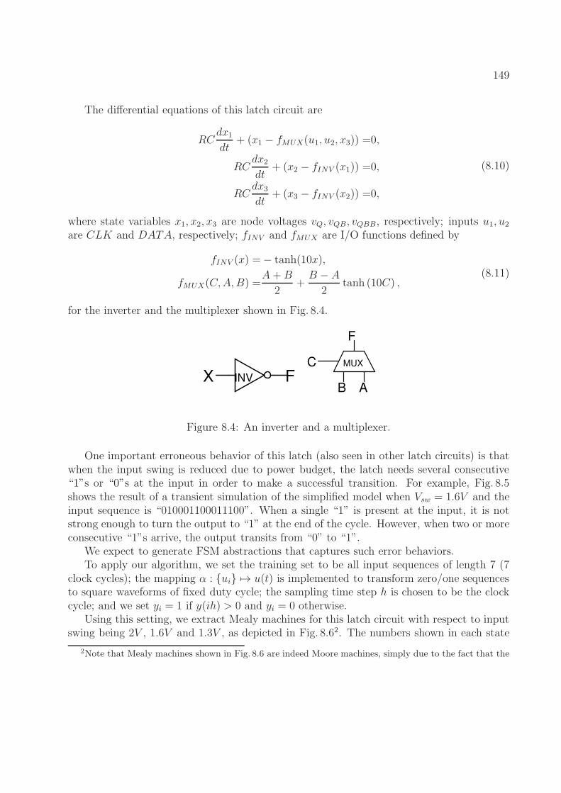
149

The differential equations of this latch circuit are

RCdx1

dt+ (x1 − fMUX(u1, u2, x3)) =0,

RCdx2

dt+ (x2 − fINV (x1)) =0,

RCdx3

dt+ (x3 − fINV (x2)) =0,

(8.10)

where state variables x1, x2, x3 are node voltages vQ, vQB, vQBB, respectively; inputs u1, u2

are CLK and DATA, respectively; fINV and fMUX are I/O functions defined by

fINV (x) =− tanh(10x),

fMUX(C,A,B) =A +B

2+

B − A

2tanh (10C) ,

(8.11)

for the inverter and the multiplexer shown in Fig. 8.4.

INVX FMUXC

B A

F

Figure 8.4: An inverter and a multiplexer.

One important erroneous behavior of this latch (also seen in other latch circuits) is thatwhen the input swing is reduced due to power budget, the latch needs several consecutive“1”s or “0”s at the input in order to make a successful transition. For example, Fig. 8.5shows the result of a transient simulation of the simplified model when Vsw = 1.6V and theinput sequence is “010001100011100”. When a single “1” is present at the input, it is notstrong enough to turn the output to “1” at the end of the cycle. However, when two or moreconsecutive “1”s arrive, the output transits from “0” to “1”.

We expect to generate FSM abstractions that captures such error behaviors.To apply our algorithm, we set the training set to be all input sequences of length 7 (7

clock cycles); the mapping α : ui 7→ u(t) is implemented to transform zero/one sequencesto square waveforms of fixed duty cycle; the sampling time step h is chosen to be the clockcycle; and we set yi = 1 if y(ih) > 0 and yi = 0 otherwise.

Using this setting, we extract Mealy machines for this latch circuit with respect to inputswing being 2V , 1.6V and 1.3V , as depicted in Fig. 8.62. The numbers shown in each state

2Note that Mealy machines shown in Fig. 8.6 are indeed Moore machines, simply due to the fact that the

150

Figure 8.5: Response of the latch when the input sequence is “10011000001001100000” andVsw = 1.6V .

are not arbitrary. They are values of rows in the observation table, i.e., the quantized outputwith respect to corresponding input sequences. As an example, the observation table of thelatch with input swing 1.6 is shown in Table 8.2. We see that the state “0,0,0,0” correspondsto row λ, the state “0,0,1,0” corresponds to row “1”, etc.. From Table 8.2, we can derive theFSM in Fig. 8.6(b) using (8.9).

Based on the Mealy machines in Fig. 8.6, we can claim that when input swing is 2V , thelatch behaves like an ideal latch; when input swing is 1.6V , the input signal must persistfor two consecutive cycles to avoid errors; when input swing is 1.3V , the input signal mustpersist for three consecutive cycles to avoid errors. These properties can either be directlyobserved in simple FSMs, or be checked by model checking tools. To validate these claims, weperform many further SPICE simulations, and the same qualitative behaviors are observed.

Using these Mealy machines, we then construct Voronoi diagrams using discrete pointscorresponding to each state. For example, the Voronoi diagram of the Mealy machine inFig. 8.6(b) is shown in Fig. 8.7. The four points correspond to four states in Fig. 8.6(b), andthe (blue) trajectories in Fig. 8.7 are simulation traces that leads to the discrete points ofdifferent states, and show typical transition dynamics of the latch. This partitioning of thestate space also provides direct intuition on how circuit behave: the two states at two cornersrepresent solid “0” and solid “1” states; the two states in the middle capture dynamics inthe metastable region, and can be viewed as weak “0” and weak “1” states.

output y is just the output voltage which corresponds to a state variable x3. This is very common in circuitsimulations, and a simple post-processing can be performed to obtain a Moore machine.

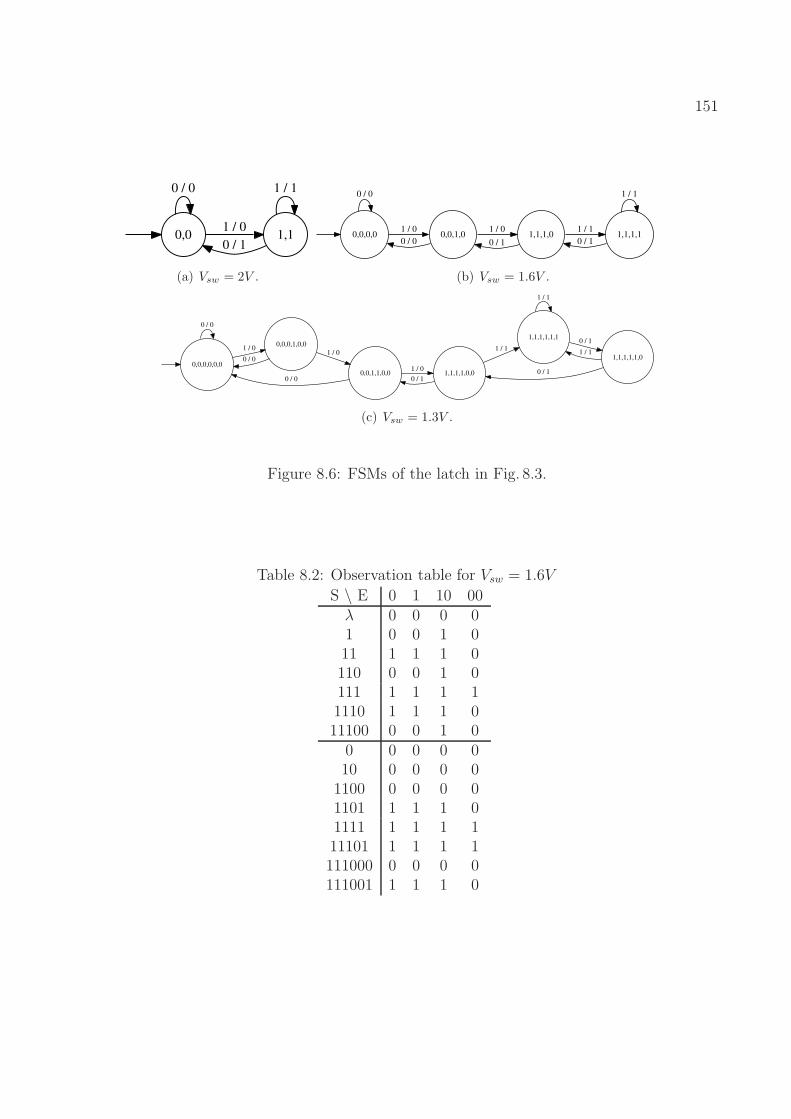
151

0,0

0 / 0

1,11 / 0

0 / 1

1 / 1

(a) Vsw = 2V .

0,0,0,0

0 / 0

0,0,1,01 / 0

0 / 01,1,1,0

1 / 0

0 / 11,1,1,1

1 / 1

0 / 1

1 / 1

(b) Vsw = 1.6V .

0,0,0,0,0,0

0 / 0

0,0,0,1,0,01 / 0

0,0,1,1,0,00 / 0

1,1,1,1,0,01 / 0

0 / 1

1,1,1,1,1,1

1 / 1

0 / 01 / 0

1,1,1,1,1,0

0 / 1

1 / 1

0 / 1

1 / 1

(c) Vsw = 1.3V .

Figure 8.6: FSMs of the latch in Fig. 8.3.

Table 8.2: Observation table for Vsw = 1.6V

S \ E 0 1 10 00λ 0 0 0 01 0 0 1 011 1 1 1 0110 0 0 1 0111 1 1 1 11110 1 1 1 011100 0 0 1 00 0 0 0 010 0 0 0 01100 0 0 0 01101 1 1 1 01111 1 1 1 111101 1 1 1 1111000 0 0 0 0111001 1 1 1 0

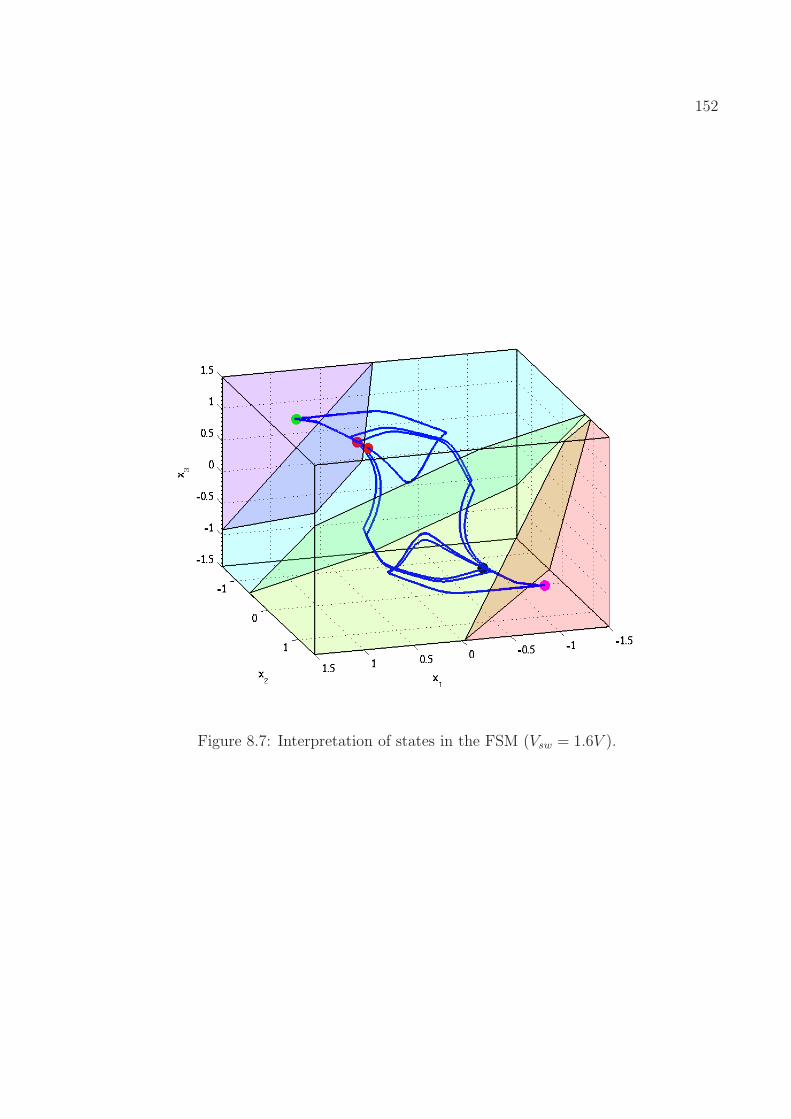
152

Figure 8.7: Interpretation of states in the FSM (Vsw = 1.6V ).

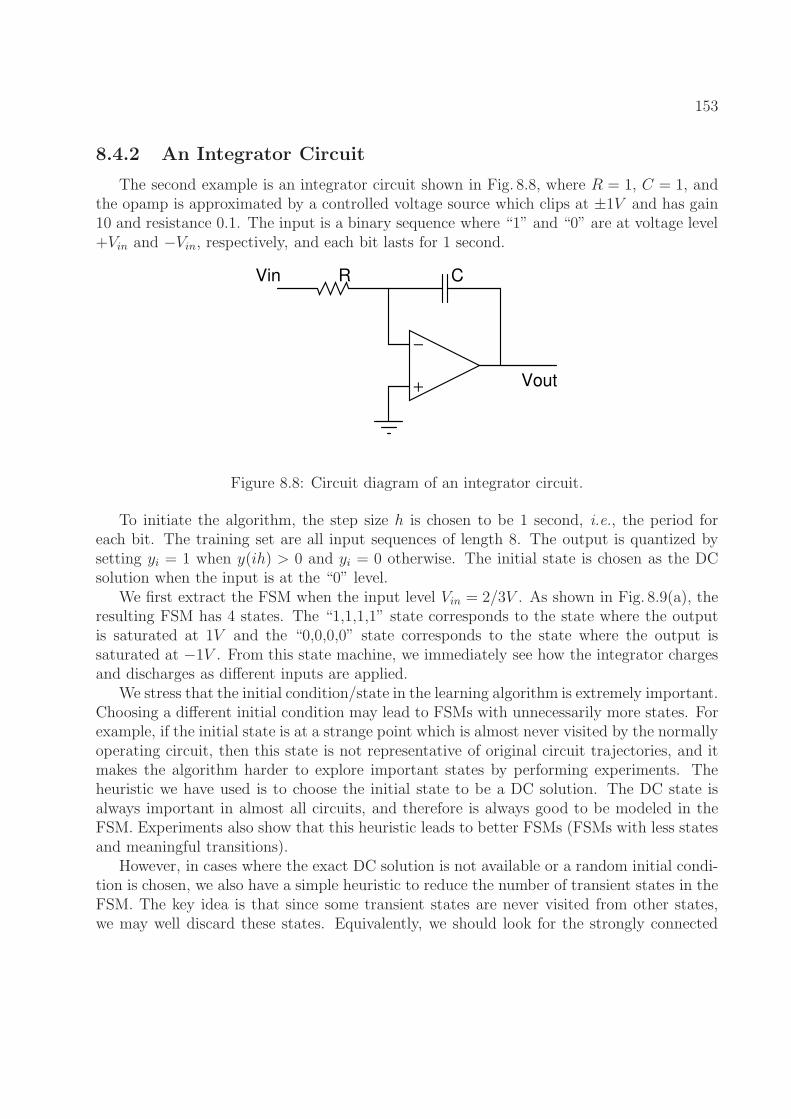
153

8.4.2 An Integrator Circuit

The second example is an integrator circuit shown in Fig. 8.8, where R = 1, C = 1, andthe opamp is approximated by a controlled voltage source which clips at ±1V and has gain10 and resistance 0.1. The input is a binary sequence where “1” and “0” are at voltage level+Vin and −Vin, respectively, and each bit lasts for 1 second.

−

+

Vin

Vout

R C

Figure 8.8: Circuit diagram of an integrator circuit.

To initiate the algorithm, the step size h is chosen to be 1 second, i.e., the period foreach bit. The training set are all input sequences of length 8. The output is quantized bysetting yi = 1 when y(ih) > 0 and yi = 0 otherwise. The initial state is chosen as the DCsolution when the input is at the “0” level.

We first extract the FSM when the input level Vin = 2/3V . As shown in Fig. 8.9(a), theresulting FSM has 4 states. The “1,1,1,1” state corresponds to the state where the outputis saturated at 1V and the “0,0,0,0” state corresponds to the state where the output issaturated at −1V . From this state machine, we immediately see how the integrator chargesand discharges as different inputs are applied.

We stress that the initial condition/state in the learning algorithm is extremely important.Choosing a different initial condition may lead to FSMs with unnecessarily more states. Forexample, if the initial state is at a strange point which is almost never visited by the normallyoperating circuit, then this state is not representative of original circuit trajectories, and itmakes the algorithm harder to explore important states by performing experiments. Theheuristic we have used is to choose the initial state to be a DC solution. The DC state isalways important in almost all circuits, and therefore is always good to be modeled in theFSM. Experiments also show that this heuristic leads to better FSMs (FSMs with less statesand meaningful transitions).

However, in cases where the exact DC solution is not available or a random initial condi-tion is chosen, we also have a simple heuristic to reduce the number of transient states in theFSM. The key idea is that since some transient states are never visited from other states,we may well discard these states. Equivalently, we should look for the strongly connected

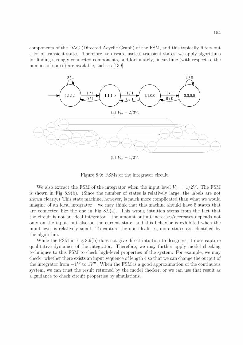
154

components of the DAG (Directed Acyclic Graph) of the FSM, and this typically filters outa lot of transient states. Therefore, to discard useless transient states, we apply algorithmsfor finding strongly connected components, and fortunately, linear-time (with respect to thenumber of states) are available, such as [139].

1,1,1,1

0 / 1

1,1,1,01 / 1

0 / 11,1,0,0

1 / 1

0 / 10,0,0,0

1 / 1

0 / 0

1 / 0

(a) Vin = 2/3V .

1,1,1,1,1,1,1,1,1,1,0,1,1,1,1

1,1,1,1,0,0,1,0,1,1,0,1,1,1,1

1 / 1

1,1,1,1,1,0,1,1,1,1,1,1,1,1,1

0 / 1

1,1,0,0,0,0,1,0,1,1,0,1,1,1,1

0,0,0,0,0,0,0,0,1,1,0,0,1,1,0

1 / 1

1,1,1,1,0,0,1,1,1,1,0,1,1,1,1

0 / 1 0,0,0,0,0,0,0,0,0,1,0,0,1,0,0

1 / 0

1,1,1,0,0,0,1,0,1,1,0,0,1,1,10 / 0

0 / 1

1,1,1,0,0,0,1,0,1,1,0,1,1,1,11 / 1

0 / 11,1,0,0,0,0,0,0,1,1,0,0,1,1,1

1 / 1

0 / 1

0,0,0,0,0,0,0,0,0,1,0,0,1,1,0

1 / 1

0 / 0

0,0,0,0,0,0,0,0,0,0,0,0,1,0,01 / 0

0 / 0

0,0,0,0,0,0,0,0,0,0,0,0,0,0,0

1 / 0

0 / 0

1 / 0

1,1,0,0,0,0,0,0,1,1,0,0,1,1,0

1 / 1

0 / 1

1,1,1,1,0,0,1,1,1,1,1,1,1,1,1

0 / 1

1,1,1,0,0,0,1,1,1,1,0,1,1,1,11 / 1

1 / 1

0 / 1

0 / 0

1 / 0

0 / 1

1 / 1

0 / 1

1,1,1,0,0,0,0,0,1,1,0,1,1,1,1

1 / 1

0 / 1

1 / 1

1 / 1

0 / 1

(b) Vin = 1/2V .

Figure 8.9: FSMs of the integrator circuit.

We also extract the FSM of the integrator when the input level Vin = 1/2V . The FSMis shown in Fig. 8.9(b). (Since the number of states is relatively large, the labels are notshown clearly.) This state machine, however, is much more complicated than what we wouldimagine of an ideal integrator – we may think that this machine should have 5 states thatare connected like the one in Fig. 8.9(a). This wrong intuition stems from the fact thatthe circuit is not an ideal integrator – the amount output increases/decreases depends notonly on the input, but also on the current state, and this behavior is exhibited when theinput level is relatively small. To capture the non-idealities, more states are identified bythe algorithm.

While the FSM in Fig. 8.9(b) does not give direct intuition to designers, it does capturequalitative dynamics of the integrator. Therefore, we may further apply model checkingtechniques to this FSM to check high-level properties of the system. For example, we maycheck “whether there exists an input sequence of length 4 so that we can change the output ofthe integrator from −1V to 1V ”. When the FSM is a good approximation of the continuoussystem, we can trust the result returned by the model checker, or we can use that result asa guidance to check circuit properties by simulations.

155

Chapter 9

Conclusion and Future Work

Model order reduction for nonlinear dynamical systems has been a difficult problem formany years. This dissertation provides a self-contained view of the MOR problem, andpresents several algorithms, ManiMOR, QLMOR, NTIM, DAE2FSM, to solve the problemfrom different perspectives.

Starting with the linear projection framework used by most previous techniques, we studyand analyze its drawbacks in applications to reduce nonlinear systems. With that, we presenta more general nonlinear projection framework which we believe is the natural and correctframework for nonlinear model order reduction. Indeed, the techniques presented in previouschapters may all be interpreted in this framework.

In its most straightforward form, we have presented ManiMOR which explicitly con-structs and parameterizes a nonlinear manifold, and projects the full model on the manifoldto obtain a reduced model. The projected model, by construction, matches the DC andAC responses of the full model, and can be proven to be much more efficient than linearprojection-based methods.

By exploiting internal structures of the full model, we have proposed QLMOR whichcreates a QLDAE reduced model. The key contribution of this work is the development of asymbolic transformation procedure that creates an equivalent quadratic-linear model to thefull model. By doing so, it has avoided all problems caused by Taylor series truncation, suchas local convergence, high computational cost, passivity/stability loss, etc.. The other keycontribution is the development of a reduction algorithm of QLDAEs which guarantees tomatch certain moments of the Volterra kernel for QLDAEs. Therefore, this reduced modelis especially of great use for capturing harmonic distortions in nonlinear systems.

Using a very specific nonlinear manifold/projection, we have presented NTIM, a phasemacromodel that is proven to capture phase responses in nonlinear systems. While we de-velop the model using Floquet theory, the phase macromodel naturally fits into the nonlinearprojection framework. Due to the importance of timing/phase responses in practical systems,this model is shown to be useful in many scenarios.

Besides reduced order models in the form of differential equations, we also try to see if

156

other types of reduced models are appropriate. In particular, we presented DAE2FSM thatabstracts a finite state machine from a set of differential equations. This model is especiallyuseful if the full model behaves as a finite state machine – in that case, the algorithmguarantees to find the corresponding finite state machine. FSMmodels can be further fed intomodel checking tools to verify higher-level system properties, and have various applicationssuch as mixed-signal system simulation and biological system abstraction.

Rather than completely solving the nonlinear MOR problem, our exploration leads tomany more research directions to pursue. In the following, we comment on further improve-ments that may be done for the methods we present in this dissertation. We then sketch afew potential theoretical and practical improvements/extensions/considerations.

9.1 Future Work on Proposed Methods

9.1.1 ManiMOR

1. The Krylov distribution defined by (4.22) is generally not involutive. However, thereare systems of which (4.22) is involutive. It is interesting to see what systems have suchproperties and what such properties correspond to in real circuit implementations.

2. By construction, ManiMOR ensures that the DC attractors are included in the mani-fold. This satisfies the necessary condition that the reduced order model can reproduceattractors of the full model. However, this is not sufficient for the stability to be pre-served. It is useful to show under what conditions can the stability be preserved.

3. In the derivation of ManiMOR, we have assumed that f(·) in the differential equationsis invertible. However, this does not always hold. For example, in bi-stable systemssuch as SRAMs, one DC input corresponds to two stable DC solutions. One possiblesolution is to find a manifold that covers all DC solutions. Another possible solution isto modify the circuit to a decoupled (open-loop) one such that f(·) becomes invertible,and then reduce the open-loop model.

4. MIMO systems may be handled by generalizing the manifold definition. For example,the DC manifold, which is a one-dimensional manifold for SIMO models, may bedefined as a manifold of larger size. For example, Fig. 9.1 shows a 2-input NANDcircuit and the 2-dimensional DC manifold. Following this idea, we may also extendthe definition of AC and ManiMOR manifolds.

5. For oscillators, DC equilibria are not the attractors. Instead, the periodic solution,or the limit cycle in the state space is the attractor. Therefore, the definition of themanifold should be changed for oscillators. It seems that this has several connectionsto the NTIM reduced model that deserve further investigations.

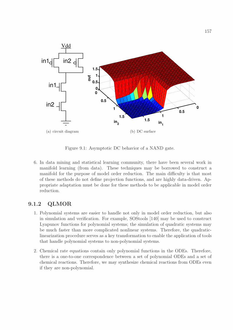
157

in1 in2

in1

in2

Vdd

(a) circuit diagram

00.5

11.5

0

0.5

1

1.5

0

0.5

1

1.5

in1

in2

ou

t

(b) DC surface

Figure 9.1: Asymptotic DC behavior of a NAND gate.

6. In data mining and statistical learning community, there have been several work inmanifold learning (from data). These techniques may be borrowed to construct amanifold for the purpose of model order reduction. The main difficulty is that mostof these methods do not define projection functions, and are highly data-driven. Ap-propriate adaptation must be done for these methods to be applicable in model orderreduction.

9.1.2 QLMOR

1. Polynomial systems are easier to handle not only in model order reduction, but alsoin simulation and verification. For example, SOStools [140] may be used to constructLyapunov functions for polynomial systems; the simulation of quadratic systems maybe much faster than more complicated nonlinear systems. Therefore, the quadratic-linearization procedure serves as a key transformation to enable the application of toolsthat handle polynomial systems to non-polynomial systems.

2. Chemical rate equations contain only polynomial functions in the ODEs. Therefore,there is a one-to-one correspondence between a set of polynomial ODEs and a set ofchemical reactions. Therefore, we may synthesize chemical reactions from ODEs evenif they are non-polynomial.

158

3. From a different perspective, the quadratic-linearization procedure shows that anynonlinear system may be written as a QLDAE. Therefore, the QLDAE form is anacceptable form for nonlinear system identification, and it represents a nonlinear systemby matrices. We may modify current system identification methods to identify QLDAEmodels.

9.1.3 NTIM

1. NTIM in Chapter 7 generates phase models for only single-input systems. It is notapplicable to multiple-input systems because these system will settle in a quasi-periodicsteady state. From a projection view point, the manifold is no longer the limit cycle,but a torus in the state space. It appears that multiple phase variables and multiplephase equations need to be defined for systems in quasi-periodic steady states.

2. The phase model may be used in timing analysis of a large digital circuit – we mayreplace each digital gate by its phase model, therefore reducing the number of equationsdescribing each gate to 1. This greatly speeds up the simulation, while preserves timingbehaviors.

9.1.4 DAE2FSM

1. DAE2FSM learns an FSM from trajectories. An alternative is to directly construct anFSM from the differential equations. This again requires us to define an appropriatenotion of equivalence between the DAEs and the FSMs. Some initial study show thatfor simple linear or nonlinear systems, we may have rigorous definitions and efficientalgorithms. We are following this line of research, and hope to reach more generalresults and algorithms.

2. With the FSM learned, we may apply model checking or probabilistic model checkingtools to check higher-level system behaviors. In particular, for the latch circuit (to beused in a communication link), we have developed an efficient algorithm to computethe BER (bit-error rate) of the link given the finite state machine of the latch, assumingthe errors are caused by non-idealities in the latch.

3. Besides deterministic FSM learning techniques, there have also been techniques tolearn non-deterministic or probabilistic machines. How to employ these techniques inlearning from DAE models remains a question. We are studying a few of these repre-sentative algorithms and exploring the possibility of adaptation of these algorithms.

159

9.2 Other Future Work

1. While we have mainly considered the model reduction of ODE/DAE models, the modelorder reduction of other models in Table 1.1 deserve further investigation. For example,we may reduce an FSM model by merging/removing states. The question is again whatare the “important” states, and how to identify these states. A straightforward ideais to preserve the attractors of the FSM. Similarly, we can explore the model orderreduction of other models.

2. Chemical reactions may also be viewed as a model, although it not listed in Table 1.1.While it describes chemical kinetics, it is not strictly a mathematical model because itmay be interpreted as many different models, deterministic or stochastic, finite-stateor infinite-state. The reduction of the chemical reactions is possible – by ignoring thereactions that have a high reaction rate, we may obtain a model that captures the slowkinetic dynamics. However, this method is not “optimal” generally in other senses(such as attractor-preserving, moment-matching, etc.). It is interesting to explore theapplication of other MOR techniques or develop new MOR techniques for the chemicalreactions.

3. We may also look at the problem of abstracting one model from another. For example,from an ODE/DAE model to a hybrid model. Such abstractions can have a lot ofapplications, e.g., to simplify the implementations/synthesis of a controller.

4. One important aspect of the projection framework is that it is computationally efficientto obtain a projection that leads to a reasonable reduced order model. However,recently there have been many progresses in improving the efficiency of optimizationalgorithms. The direct application of the state-of-the-art optimization routines maybe possible.

5. We have mentioned in Section 2.1.3 the problem of formal verification of analog/mixed-signal systems. However, such algorithms and tools are extremely immature, anddeserves further investigation. While this is not about model order reduction, it closelyrelates to MOR in that such tools may be used to check the correctness of reducedmodels.

6. Practical systems may be redundant. For example, the LTI system matrices may berank-deficient. It looks like MOR method may remove the redundancy in such systems.It is interesting to see if MOR methods can actually preserve certain redundancies.

7. In several structure-preserving MOR techniques, certain structures (of LTI systems)are preserved so that the reduced model corresponds to an RLC circuit implementation.A similar problem is how to obtain a nonlinear model that corresponds to a transistor-level implementation.

160

8. There have been some literature discussing how to do nonlinear balanced truncation toobtain a reduced model. However, the theory of nonlinear balancing has not reacheda consensus, and the existing methods are computationally extremely inefficient.

9. The theory for the balanced realization of LTV systems seems to be well-established.However, the circuit community have not been aware of these techniques. We may trythese techniques and see how they work for circuit examples.

10. We have shown that some nonlinear systems, under appropriate coordinate transfor-mations, may be converted to equivalent linear systems. However, the question is whywould we want to implement an LTI system using a nonlinear system? One possibil-ity is that the LTI implementation may require unrealistic resistance and capacitancevalues that cannot be mapped to an integrated circuit. In that case, it would be greatif we can map the LTI system to a nonlinear system that can be implemented on chip.

11. The sparsity is typically destroyed by MOR methods. However, the discussion inChapter 3 reveals that sometimes we have extra degree of freedom in choosing a pro-jected model. These degree of freedom may be used to achieve the sparsity of thereduced order model.

161

Bibliography

[1] R.T. Chang et al. Near Speed-of-Light Signaling Over On-chip Electrical Interconnects.Solid-State Circuits, IEEE Journal of, 38:834–838, May 2003.

[2] Michal Rewienski and Jacob White. A Trajectory Piecewise-Linear Approach to ModelOrder Reduction and Fast Simulation of Nonlinear Circuits and Micromachined De-vices. IEEE Transactions on Computer-Aided Design, 22(2), February 2003.

[3] Y. Wang and H.G. Dohlman. Pheromone Signaling Mechanisms in Yeast: A Proto-typical Sex Machine. Science, 306:1508–1509, Nov 2004.

[4] K.C. Sou, A. Megretski, and L. Daniel. A quasi-convex optimization approach toparameterized model order reduction. Computer-Aided Design of Integrated Circuitsand Systems, IEEE Transactions on, 27(3):456–469, 2008.

[5] L. Daniel, O.C. Siong, L.S. Chay, K.H. Lee, and J. White. A multiparameter moment-matching model-reduction approach for generating geometrically parameterized in-terconnect performance models. Computer-Aided Design of Integrated Circuits andSystems, IEEE Transactions on, 23(5):678–693, 2004.

[6] B.N. Bond and L. Daniel. A piecewise-linear moment-matching approach to param-eterized model-order reduction for highly nonlinear systems. Computer-Aided Designof Integrated Circuits and Systems, IEEE Transactions on, 26(12):2116–2129, 2007.

[7] P. Li, F. Liu, X. Li, L.T. Pileggi, and S.R. Nassif. Modeling interconnect variabilityusing efficient parametric model order reduction. In Proceedings of the conference onDesign, Automation and Test in Europe-Volume 2, pages 958–963. IEEE ComputerSociety, 2005.

[8] X. Li, P. Li, and L.T. Pileggi. Parameterized interconnect order reduction with explicit-and-implicit multi-parameter moment matching for inter/intra-die variations. In iccad,pages 806–812. IEEE, 2005.

[9] T. Bui-Thanh, K. Willcox, and O. Ghattas. Model reduction for large-scale systemswith high-dimensional parametric input space. SIAM Journal on Scientific Computing,30(6):3270–3288, 2008.

162

[10] Y. Liu, L.T. Pileggi, and A.J. Strojwas. Model order-reduction of RC (L) interconnectincluding variational analysis. In Proceedings of the 36th annual ACM/IEEE DesignAutomation Conference, pages 201–206. ACM, 1999.

[11] A. Odabasioglu, M. Celik, and L.T. Pileggi. PRIMA: Passive reduced-order intercon-nect macromodeling algorithm. In Proceedings of the 1997 IEEE/ACM internationalconference on Computer-aided design, pages 58–65. IEEE Computer Society, 1997.

[12] J.M. Wang, C.C. Chu, Q. Yu, and E.S. Kuh. On projection-based algorithms formodel-order reduction of interconnects. Circuits and Systems I: Fundamental Theoryand Applications, IEEE Transactions on, 49(11):1563–1585, 2002.

[13] I.M. Elfadel and D.D. Ling. A block rational Arnoldi algorithm for multipoint pas-sive model-order reduction of multiport RLC networks. In Proceedings of the 1997IEEE/ACM international conference on Computer-aided design, pages 66–71. IEEEComputer Society, 1997.

[14] Y. Shin and T. Sakurai. Power distribution analysis of VLSI interconnects using modelorder reduction. Computer-Aided Design of Integrated Circuits and Systems, IEEETransactions on, 21(6):739–745, 2002.

[15] A.C. Cangellaris, M. Celik, S. Pasha, and L. Zhao. Electromagnetic model order reduc-tion for system-level modeling. Microwave Theory and Techniques, IEEE Transactionson, 47(6):840–850, 1999.

[16] H. Wu and A.C. Cangellaris. Model-order reduction of finite-element approximations ofpassive electromagnetic devices including lumped electrical-circuit models. MicrowaveTheory and Techniques, IEEE Transactions on, 52(9):2305–2313, 2004.

[17] T. Wittig, I. Munteanu, R. Schuhmann, and T. Weiland. Two-step Lanczos algorithmfor model order reduction. Magnetics, IEEE Transactions on, 38(2):673–676, 2002.

[18] R.D. Slone, R. Lee, and J.F. Lee. Multipoint Galerkin asymptotic waveform evalu-ation for model order reduction of frequency domain FEM electromagnetic radiationproblems. Antennas and Propagation, IEEE Transactions on, 49(10):1504–1513, 2001.

[19] M.E. Kowalski and J.M. Jin. Model-order reduction of nonlinear models of electro-magnetic phased-array hyperthermia. Biomedical Engineering, IEEE Transactions on,50(11):1243–1254, 2003.

[20] H. Yu, Y. Shi, and L. He. Fast analysis of structured power grid by triangularizationbased structure preserving model order reduction. In Proceedings of the 43rd annualDesign Automation Conference, pages 205–210. ACM, 2006.

163

[21] H. Su, E. Acar, and S.R. Nassif. Power grid reduction based on algebraic multigridprinciples. 2003.

[22] T.V. Nguyen and J.M. Wang. Extended Krylov subspace method for reduced orderanalysis of linear circuits with multiple sources. In dac, pages 247–252. ACM, 2000.

[23] J. Wood, D.E. Root, and N.B. Tufillaro. A behavioral modeling approach to nonlinearmodel-order reduction for RF/microwave ICs and systems. Microwave Theory andTechniques, IEEE Transactions on, 52(9):2274–2284, 2004.

[24] P. Li and L.T. Pileggi. NORM: compact model order reduction of weakly nonlinearsystems. 2003.

[25] J.R. Phillips. Projection-based approaches for model reduction of weakly nonlinear,time-varying systems. Computer-Aided Design of Integrated Circuits and Systems,IEEE Transactions on, 22(2):171–187, 2003.

[26] X. Li, P. Li, Y. Xu, and L.T. Pileggi. Analog and RF circuit macromodels for system-level analysis. 2003.

[27] A. Zhu and T.J. Brazil. Behavioral modeling of RF power amplifiers based on prunedVolterra series. Microwave and Wireless Components Letters, IEEE, 14(12):563–565,2004.

[28] J. Roychowdhury. Reduced-order modeling of time-varying systems. Circuits andSystems II: Analog and Digital Signal Processing, IEEE Transactions on, 46(10):1273–1288, 1999.

[29] A. Demir, A. Mehrotra, and J. Roychowdhury. Phase noise in oscillators: A unifyingtheory and numerical methods for characterization. Circuits and Systems I: Funda-mental Theory and Applications, IEEE Transactions on, 47(5):655–674, 2000.

[30] X. Lai and J. Roychowdhury. TP-PPV: piecewise nonlinear, time-shifted oscillatormacromodel extraction for fast, accurate PLL simulation. In Proceedings of the 2006IEEE/ACM international conference on Computer-aided design, pages 269–274. ACM,2006.

[31] X. Lai and J. Roychowdhury. Macromodelling oscillators using Krylov-subspace meth-ods. In Proceedings of the 2006 Asia and South Pacific Design Automation Conference,pages 527–532. IEEE Press, 2006.

[32] B. Gu, K.K. Gullapalli, S. Hamm, B. Mulvaney, X. Lai, and J. Roychowdhury. Imple-menting nonlinear oscillator macromodels using Verilog-AMS for accurate predictionof injection locking behaviors of oscillators. In Behavioral Modeling and Simulation

164

Workshop, 2005. BMAS 2005. Proceedings of the 2005 IEEE International, pages 43–47. IEEE, 2005.

[33] J.S. Han, E.B. Rudnyi, and J.G. Korvink. Efficient optimization of transient dynamicproblems in MEMS devices using model order reduction. Journal of Micromechanicsand Microengineering, 15:822, 2005.

[34] J. Lienemann, E.B. Rudnyi, and J.G. Korvink. MST MEMS model order reduction:Requirements and benchmarks. Linear algebra and its applications, 415(2-3):469–498,2006.

[35] E. Rudnyi and J. Korvink. Model order reduction for large scale engineering modelsdeveloped in ANSYS. In Applied Parallel Computing, pages 349–356. Springer, 2006.

[36] J. Chen and S.M. Kang. Model-order reduction of nonlinear mems devices througharclength-based Karhunen-Loeve decomposition. In Circuits and Systems, 2001. IS-CAS 2001. The 2001 IEEE International Symposium on, volume 3, pages 457–460.IEEE, 2001.

[37] E.B. Rudnyi and J.G. Korvink. Review: Automatic Model Reduction for TransientSimulation of MEMS-based Devices. Sensors Update, 11(1):3–33, 2002.

[38] YC Liang, WZ Lin, HP Lee, SP Lim, KH Lee, and H. Sun. Proper orthogonal decom-position and its applications-part II: Model reduction for MEMS dynamical analysis.Journal of Sound and Vibration, 256(3):515–532, 2002.

[39] P. Benner, V. Mehrmann, and D.C. Sorensen. Dimension reduction of large-scalesystems. 2005.

[40] K. Willcox and J. Peraire. Balanced model reduction via the proper orthogonal de-composition. AIAA journal, 40(11):2323–2330, 2002.

[41] P.V. Kokotovic et al. Singular perturbations and order reduction in control theory–anoverview. Automatica, 12(2):123–132, 1976.

[42] M. Bordemann and J. Hoppe. The Dynamics of Relativistic Membranes I: Reductionto 2-dimensional Fluid Dynamics. Arxiv preprint hep-th/9307036, 1993.

[43] C.W. Rowley, T. Colonius, and R.M. Murray. Model reduction for compressible flowsusing POD and Galerkin projection. Physica D: Nonlinear Phenomena, 189(1-2):115–129, 2004.

[44] B.F. Farrell and P.J. Ioannou. Accurate low-dimensional approximation of the lineardynamics of fluid flow. Journal of the atmospheric sciences, 58(18):2771–2789, 2001.

165

[45] X. Ma and G.E. Karniadakis. A low-dimensional model for simulating three-dimensional cylinder flow. Journal of Fluid Mechanics, 458(-1):181–190, 2002.

[46] B.R. Noack, M. Schlegel, M. Morzynski, and G. Tadmor. System reduction strategyfor Galerkin models of fluid flows. International Journal for Numerical Methods inFluids, 63(2):231–248, 2010.

[47] I.K. Fodor. A survey of dimension reduction techniques. Center for Applied ScientificComputing, Lawrence Livermore National Laboratory, 2002.

[48] K.R. Schneider and T. Wilhelm. Model reduction by extended quasi-steady-stateapproximation. Journal of mathematical biology, 40(5):443–450, 2000.

[49] C.W. Rowley, I.G. Kevrekidis, J.E. Marsden, and K. Lust. Reduction and reconstruc-tion for self-similar dynamical systems. Nonlinearity, 16:1257, 2003.

[50] D. Lebiedz, V. Reinhardt, and J. Kammerer. Novel trajectory based concepts for modeland complexity reduction in (bio) chemical kinetics. Model Reduction and Coarse-Graining Approaches for Multiscale Phenomena, pages 343–364.

[51] S. Danø, M.F. Madsen, H. Schmidt, and G. Cedersund. Reduction of a biochemicalmodel with preservation of its basic dynamic properties. FEBS Journal, 273(21):4862–4877, 2006.

[52] T.B. Kepler, LF Abbott, and E. Marder. Reduction of conductance-based neuronmodels. Biological Cybernetics, 66(5):381–387, 1992.

[53] D. Golomb, J. Guckenheimer, and S. Gueron. Reduction of a channel-based model fora stomatogastric ganglion LP neuron. Biological cybernetics, 69(2):129–137, 1993.

[54] W.M. Kistler, W. Gerstner, and J.L. Hemmen. Reduction of the Hodgkin-Huxleyequations to a single-variable threshold model. Neural Computation, 9(5):1015–1045,1997.

[55] E.M. Izhikevich. Simple model of spiking neurons. Neural Networks, IEEE Transac-tions on, 14(6):1569–1572, 2003.

[56] D. Hansel, G. Mato, and C. Meunier. Phase dynamics for weakly coupled Hodgkin-Huxley neurons. EPL (Europhysics Letters), 23:367, 1993.

[57] Y. Maeda, K. Pakdaman, T. Nomura, S. Doi, and S. Sato. Reduction of a model foran Onchidium pacemaker neuron. Biological cybernetics, 78(4):265–276, 1998.

[58] B. Cartling. Response characteristics of a low-dimensional model neuron. Neuralcomputation, 8(8):1643–1652, 1996.

166

[59] K. Doya and A.I. Selverston. Dimension reduction of biological neuron models byartificial neural networks. Neural Computation, 6(4):696–717, 1994.

[60] S. Peles, B. Munsky, and M. Khammash. Reduction and solution of the chemicalmaster equation using time scale separation and finite state projection. The Journalof chemical physics, 125:204104, 2006.

[61] L. Petzold and W. Zhu. Model reduction for chemical kinetics: An optimizationapproach. AIChE journal, 45(4):869–886, 1999.

[62] M.S. Okino and M.L. Mavrovouniotis. Simplification of mathematical models of chem-ical reaction systems. Chemical reviews, 98(2):391–408, 1998.

[63] D. Lebiedz. Computing minimal entropy production trajectories: An approach tomodel reduction in chemical kinetics. The Journal of chemical physics, 120:6890, 2004.

[64] S. Lall, J.E. Marsden, and S. Glavaski. A subspace approach to balanced truncationfor model reduction of nonlinear control systems. International Journal of Robust andNonlinear Control, 12(6):519–535, 2002.

[65] U. Maas and S.B. Pope. Simplifying chemical kinetics: intrinsic low-dimensional man-ifolds in composition space. Combustion and Flame, 88(3-4):239–264, 1992.

[66] Z. Ren, S.B. Pope, A. Vladimirsky, and J.M. Guckenheimer. The invariant constrainedequilibrium edge preimage curve method for the dimension reduction of chemical ki-netics. The Journal of chemical physics, 124:114111, 2006.

[67] E.A. Mastny, E.L. Haseltine, and J.B. Rawlings. Two classes of quasi-steady-statemodel reductions for stochastic kinetics. The Journal of chemical physics, 127:094106,2007.

[68] G. Kerschen, J.C. Golinval, A.F. Vakakis, and L.A. Bergman. The method of properorthogonal decomposition for dynamical characterization and order reduction of me-chanical systems: an overview. Nonlinear Dynamics, 41(1):147–169, 2005.

[69] S. Lall, P. Krysl, and J.E. Marsden. Structure-preserving model reduction for mechan-ical systems. Physica D: Nonlinear Phenomena, 184(1-4):304–318, 2003.

[70] P. Koutsovasilis and M. Beitelschmidt. Comparison of model reduction techniques forlarge mechanical systems. Multibody System Dynamics, 20(2):111–128, 2008.

[71] V. Duindam and S. Stramigioli. Energy-based model-reduction of nonholonomic me-chanical systems. In Robotics and Automation, 2004. Proceedings. ICRA’04. 2004IEEE International Conference on, volume 5, pages 4584–4589. IEEE, 2004.

167

[72] T. Kailath. Linear systems, volume 1. Prentice-Hall Englewood Cliffs, NJ, 1980.

[73] S. Sastry. Nonlinear systems: analysis, stability, and control. Springer Verlag, 1999.

[74] A. Odabasioglu, M. Celik, and L. T. Pileggi. Prima: passive reduced-order interconnectmacromodeling algorithm. 17(8):645–654, 1998.

[75] C. Gu and J. Roychowdhury. ManiMOR: Model Reduction via Projection onto Non-linear Manifolds, with Applications to Analog Circuits and Biochemical Systems. InProceedings of the IEEE International Conference on Computer Aided Design, 10-13Nov. 2008.

[76] C. Gu. QLMOR: a New Projection-Based Approach for Nonlinear Model Order Re-duction. In Proceedings of the IEEE International Conference on Computer AidedDesign, 2-5 Nov. 2009.

[77] C. Gu and J. Roychowdhury. Generalized Nonlinear Timing/Phase Macromodeling:Theory, Numerical Methods and Applications. In Proceedings of the IEEE Interna-tional Conference on Computer Aided Design, 7-11 Nov. 2010.

[78] C. Gu and J. Roychowdhury. FSM Model Abstraction for Analog/Mixed-Signal Cir-cuits by Learning from I/O Trajectories. Proc. IEEE Asia and South Pacific DesignAutomation Conference, 2011.

[79] S. Gupta, B. H. Krogh, and R. A. Rutenbar. Towards formal verification of analogdesigns. In Proc. ICCAD-2004 Computer Aided Design IEEE/ACM Int. Conf, pages210–217, 2004.

[80] S. Blouin. Finite-state machine abstractions of continuous systems. PhD thesis,Queen’s University, 2003.

[81] P. Ye, E. Entcheva, R. Grosu, and S.A. Smolka. Efficient modeling of excitable cellsusing hybrid automata. In Proc. of CMSB, pages 216–227. Citeseer, 2005.

[82] E. Asarin, T. Dang, and A. Girard. Hybridization methods for the analysis of nonlinearsystems. Acta Informatica, 43(7):451–476, 2007.

[83] R. Alur, T.A. Henzinger, G. Lafferriere, and G.J. Pappas. Discrete abstractions ofhybrid systems. Proceedings of the IEEE, 88(7):971–984, 2000.

[84] J. Raisch and S.D. O’Young. Discrete approximation and supervisory control of con-tinuous systems. Automatic Control, IEEE Transactions on, 43(4):569–573, 1998.

[85] M.T. Heath. Scientific computing. McGraw-Hill, 1997.

168

[86] R.K. Brayton. Logic minimization algorithms for VLSI synthesis. Springer, 1984.

[87] S. Devadas, A. Ghosh, and K. Keutzer. Logic synthesis. McGraw-Hill, Inc. New York,NY, USA, 1994.

[88] R. Harjani, R.A. Rutenbar, and L.R. Carley. OASYS: A framework for analog circuitsynthesis. Computer-Aided Design of Integrated Circuits and Systems, IEEE Transac-tions on, 8(12):1247–1266, 1989.

[89] E.J. Grimme. Krylov Projection Methods for Model Reduction. PhD thesis, Universityof Illinois, EE Dept, Urbana-Champaign, 1997.

[90] B.N. Bond. Stability-Preserving Model Reduction for Linear and Nonlinear SystemsArising in Analog Circuit Applications. PhD thesis, Massachusetts Institute of Tech-nology, 2010.

[91] B.N. Bond and L. Daniel. Guaranteed stable projection-based model reduction forindefinite and unstable linear systems. In Proceedings of the 2008 IEEE/ACM Inter-national Conference on Computer-Aided Design, pages 728–735. IEEE Press, 2008.

[92] S.K. Tiwary, A. Gupta, J.R. Phillips, C. Pinello, and R. Zlatanovici. fSpice: a booleansatisfiability based approach for formally verifying analog circuits. In Proc. Workshopon Formal Verification of Analog Circuits (FAC), Princeton, 2008.

[93] S.K. Tiwary, A. Gupta, J.R. Phillips, C. Pinello, and R. Zlatanovici. First stepstowards SAT-based formal analog verification. In Proceedings of the 2009 InternationalConference on Computer-Aided Design, pages 1–8. ACM, 2009.

[94] A. Singh and P. Li. On behavioral model equivalence checking for large analog/mixedsignal systems. In Computer-Aided Design (ICCAD), 2010 IEEE/ACM InternationalConference on, pages 55–61. IEEE.

[95] David C. Walter. Verification of Analog and Mixed-Signal Circuits Using SymbolicMethods. PhD thesis, University of Utah, ECE Dept, 2007.

[96] Scott Little. Efficient Modeling and Verification of Analog/Mixed-Signal Circuits UsingLabeled Hybrid Petri Nets. PhD thesis, University of Utah, ECE Dept, 2008.

[97] L. Ljung and E.J. Ljung. System identification: theory for the user, volume 280.Prentice-Hall Upper Saddle River, NJ, 1987.

[98] Rolf Isermann and Marco Mnchhof. Identification of Dynamic Systems: An Introduc-tion with Applications. Springer, 2011.

[99] G.A. Baker and P.R. Graves-Morris. Pade approximants. Cambridge Univ Pr, 1996.

169

[100] L.T. Pillage and R.A. Rohrer. Asymptotic waveform evaluation for timing analysis.IEEE Transactions on Computer-Aided Design, 9:352–366, April 1990.

[101] P. Feldmann and R.W. Freund. Efficient linear circuit analysis by Pade approximationvia the Lanczos process. Computer-Aided Design of Integrated Circuits and Systems,IEEE Transactions on, 14(5):639–649, 1995.

[102] G.H. Golub and C.F. Van Loan. Matrix computations. Johns Hopkins Univ Pr, 1996.

[103] Y. Saad. Iterative methods for sparse linear systems. Society for Industrial Mathemat-ics, 2003.

[104] Bruce Moore. Principal Component Analysis in Linear Systems: Controllability, Ob-servability, and Model Reduction. IEEE Trans. Automatic Control, 26:17–32, February1981.

[105] W. Rugh. Nonlinear System Theory - The Volterra-Wiener Approach. Johns HopkinsUniv Press, 1981.

[106] P. Li and L.T. Pileggi. Compact reduced-order modeling of weakly nonlinear analogand rf circuits. Computer-Aided Design of Integrated Circuits and Systems, IEEETransactions on, 24(2):184–203, 2005.

[107] Joel R. Phillips. Projection-Based Approaches for Model Reduction of Weakly Nonlin-ear Time-Varying Systems. IEEE Transactions on Computer-Aided Design, 22(2):171–187, 2003.

[108] L. Pillage. Electronic circuit and system simulation methods. McGraw-Hill Profes-sional, 1998.

[109] J. Roychowdhury. Numerical Simulation and Modelling of Electronic and BiochemicalSystems. Foundations and Trends R© in Electronic Design Automation, 3(2-3):97–303,2008.

[110] D. Garfinkel, L. Garfinkel, M. Pring, S.B. Green, and B. Chance. Computer applica-tions to biochemical kinetics. Annual Review of Biochemistry, 39(1):473–498, 1970.

[111] P.A. Absil, R. Mahony, and R. Sepulchre. Optimization algorithms on matrix mani-folds. Princeton Univ Pr, 2008.

[112] J.M. Lee. Introduction to smooth manifolds. Springer Verlag, 2003.

[113] M. Spivak and M. Spivak. A comprehensive introduction to differential geometry.1979.

170

[114] Dmitry Vasilyev, Michal Rewienski, and Jacob White. A TBR-based TrajectoryPiecewise-Linear Algorithm for Generating Accurate Low-order Models for NonlinearAnalog Circuits and MEMS. Proceedings of the IEEE Design Automation Conference,2003.

[115] J. Savoj and B. Razavi. A 10-Gb/s CMOS clock and data recovery circuit with ahalf-rate linear phase detector. IEEE Journal of Solid-State Circuits, 36:761–768, May2001.

[116] Ning Dong and Jaijeet Roychowdhury. Piecewise Polynomial Nonlinear Model Reduc-tion. Proceedings of the IEEE Design Automation Conference, 2003.

[117] Ning Dong and Jaijeet Roychowdhury. Automated Nonlinear Macromodelling of Out-put Buffers for High-Speed Digital Applications. Proceedings of the IEEE DesignAutomation Conference, 2005.

[118] BSIM3. http://www-device.eecs.berkeley.edu/˜bsim3.

[119] B. Kofahl and E. Klipp. Modelling the dynamics of the yeast pheromone pathway.Yeast, 21:831–850, 2004.

[120] T.M. Thomson and D. Endy. Rapid Characterization of Cellular Pathways UsingTime-Varying Signals. In Sixth International Conference on Systems Biology, Oct2005.

[121] J. Roychowdhury. Reduced-order modelling of time-varying systems. IEEETrans. Ckts. Syst. – II: Sig. Proc., 46(10), November 1999.

[122] T. Sakurai and A.R. Newton. Alpha-power law MOSFET model and its applicationsto CMOS inverter delay and other formulas. Solid-State Circuits, IEEE Journal of,25(2):584–594, 1990.

[123] G. Gildenblat, X. Li, W. Wu, H. Wang, A. Jha, R. van Langevelde, G.D.J. Smit, A.J.Scholten, and D.B.M. Klaassen. PSP: An advanced surface-potential-based MOSFETmodel for circuit simulation. Electron Devices, IEEE Transactions on, 53(9):1979–1993, 2006.

[124] J. Shawe-Taylor and N. Cristianini. Kernel methods for pattern analysis. CambridgeUniv Pr, 2004.

[125] H. Shichman and D.A. Hodges. Modeling and simulation of insulated-gate field-effecttransistor switching circuits. Solid-State Circuits, IEEE Journal of, 3(3):285–289, 1968.

[126] D.L. Boley. Krylov space methods on state-space control models. IEEETrans. Ckts. Syst. – II: Sig. Proc., 13(6):733–758, 1994.

171

[127] J. Phillips. Model Reduction of Time-Varying Linear Systems Using Approximate Mul-tipoint Krylov-Subspace Projectors. In Proceedings of the IEEE International Confer-ence on Computer Aided Design, November 1998.

[128] G. Hachtel, R. Brayton, and F. Gustavson. The sparse tableau approach to networkanalysis and design. Circuit Theory, IEEE Transactions on, 18(1):101–113, 1971.

[129] E.M. Izhikevich. Dynamical systems in neuroscience: The geometry of excitability andbursting. The MIT press, 2007.

[130] A. Demir. Floquet theory and non-linear perturbation analysis for oscillators withdifferential-algebraic equations. International journal of circuit theory and applications,28(2):163–185, 2000.

[131] E.A. Coddington and N. Levinson. Theory of ordinary differential equations. TataMcGraw-Hill, 1972.

[132] K.S. Kundert, J.K. White, and A. Sangiovanni-Vincentelli. Steady-state methods forsimulating analog and microwave circuits. Kluwer Academic Publishers, 1990.

[133] A. Demir and J. Roychowdhury. A reliable and efficient procedure for oscillator PPVcomputation, with phase noise macromodeling applications. Computer-Aided Designof Integrated Circuits and Systems, IEEE Transactions on, 22(2):188–197, 2003.

[134] K. Tsumoto, H. Kitajima, T. Yoshinaga, K. Aihara, and H. Kawakami. Bifurcationsin Morris-Lecar neuron model. Neurocomputing, 69(4-6):293–316, 2006.

[135] D. Angluin. Learning regular sets from queries and counterexamples* 1. Informationand computation, 75(2):87–106, 1987.

[136] K. Li, R. Groz, and M. Shahbaz. Integration testing of components guided by incremen-tal state machine learning. In Testing: Academic and Industrial Conference-PracticeAnd Research Techniques, 2006. TAIC PART 2006. Proceedings, pages 59–70. IEEE,2006.

[137] M. De Berg, O. Cheong, M. Van Kreveld, and M. Overmars. Computational geometry:algorithms and applications. Springer-Verlag New York Inc, 2008.

[138] G.J. Pappas. Hybrid systems: Computation and abstraction. PhD thesis, UNIVER-SITY of CALIFORNIA, 1998.

[139] B. Aspvall. A linear-time algorithm for testing the truth of certain quantified booleanformulas. Inform. Process. Lett., 8:121–123, 1979.

172

[140] S. Prajna, A. Papachristodoulou, P. Seiler, and P. A. Parrilo. SOSTOOLS: Sum ofsquares optimization toolbox for MATLAB, 2004.

[141] B. law Jakubczyk. Introduction to Geometric Nonlinear Control; Controllability andLie Bracket.

[142] Michal Rewienski. A Trajectory Piecewise-Linear Approach to Model Order Reductionof Nonlinear Dynamical Systems. PhD thesis, MIT, 2003.

173

Appendix A

Introduction of Differential Geometry

The following introduction is based on notes in [141].

A.1 Vector Fields and Flows

Let X be an open set of RN . We denote TpX the space of tangent vectors to X at thepoint p.

A vector field on X is a mapping

p ∈ X −→ f(p) ∈ TpX, (A.1)

which assigns a tangent vector at p to any point p in X . In a given coordinate system, f isexpressed as a column vector f = (f1, · · · , fN)T .

For any vector field, we can write the differential equation

x = f(x). (A.2)

Then starting from a point p, the solution of (A.2), is denoted by a map (t, p) 7→ γt(p). Thefamily γt of local maps are called the flow of the vector field f . The following propertieshold for γt(p):

γt1 γt2 = γt1+t2 , γ−t = (γt)−1, γ0 = id. (A.3)

If ∀t, p, γt(p) are well-defined, the f is called complete, and its flow forms a one-parameter group of diffeomorphisms of X . On the other hand, given any γt(p), we candefine a unique vector field f(p) by

f(p) =∂

∂t

∣

∣

∣

∣

t=0

γt(p). (A.4)

We will denote the flow of f by γft or exp(tf).

174

A.2 Lie Bracket and its Properties

The Lie bracket of two vector fields is another vector field which, roughly speaking,measures the non-commutativeness of the flows of both vector fields. Non-commutativenessmeans the dependence of the result of applying these flows.

There are several definitions (interpretations) of the Lie bracket:Given a coordinate system, the Lie bracket of two vector fields f and g, denoted by [f, g]

is

[f, g](x) =∂g

∂x(x)f(x)− ∂f

∂x(x)g(x). (A.5)

We will call this the Jacobian definition of Lie bracket.

Proposition A.2.1 The Lie bracket of vector fields f and g is equal identically to zero ifand only if their flows commute, i.e.,

[f, g] ≡ 0 ⇔ γft γg

s (p) = γgs γf

t (p), ∀s, t ∈ RN , ∀p ∈ X. (A.6)

Two vector fields having the property in (A.6) are called commuting.

Proposition A.2.2 Consider a curve α(t) = γg−t γf

−t γgt γf

t (p). Then we have that itsfirst derivative at zero vanishes, α′(0) = 0, and the second derivative is given by the Liebracket α′′(0) = 2[f, g](p).

A.3 Coordinate Changes and Lie Bracket

We consider a global diffeomorphism Φ : X → X . Since tangent vectors are transformedthrough the Jacobian map of a diffeomorphism, the diffeomorphism defines a transformationof a vector field f

AdΦ(f)(p) = DΦ(q)f(q), q = Φ−1(p), (A.7)

where DΦ is the tangent map of Φ which in coordinates, is ∂Φ∂x. We also write

Φ∗f = AdΦf (A.8)

Note that the coordinate change p = Φ(q) transforms the differential equations p = f(p)to q = AdΦf(q). We also have AdΦ(λ1f1 + λ2f2) = λ1AdΦ(f1) + λ2AdΦ(f2), and AdΦΨ =AdΦAdΨ(f).

Proposition A.3.1 Consider the vector field AdΦ(f). The local flow of this vector field is

σt = Φ γt Φ−1. (A.9)

175

Geometric definition of Lie bracket: we define the Lie bracket of f and g as thederivative with respect t, at t = 0, of the vector field g transformed by the flow of f , i.e., wedefine

[f, g](p) =∂

∂tDγf

−t(γft (p))g(γ

ft (p)) =

∂

∂t(Adγf

−tg)(p). (A.10)

Proposition A.3.2 If Φ is a diffeomorphism of X, then

[AdΦf,AdΦg] = AdΦ[f, g]. (A.11)

In the following, we will also use adfg for [f, g], therefore adf is a linear operator in thespace of vector fields V (X). We also denote

ad0fg = g, adi

fg = adf · · · adfg. (A.12)

Proposition A.3.3 If the vector fields f and g are real analytic, then we have the followingexpansion formula for the vector field g transformed by the flow of the vector field f :

(Adγftg)(p) =

∞∑

i=0

(−t)ii!

(adifg)(p), (A.13)

where the series converges absolutely for t in a neighborhood of zero.

A.4 Vector Fields as Differential Operators

A smooth vector field f onX defines a linear operator Lf on the space of smooth functionsC∞(X) in the following way

(Lfφ)(p) =∂

∂t

∣

∣

∣

∣

t=0

φ(γft (p)) =

n∑

i=1

fi(p)∂

∂xi

φ(p). (A.14)

The operator is called directional derivative along f or Lie derivative along f .Any differential operator of order one can be written as

L =

n∑

i=1

ai(x)∂

∂xi, (A.15)

and it defines a unique vector field defined by f = (a1(x), · · · , an(x))T . Therefore, there is aone-to-one correspondence between the vector field f and the differential operator Lf .

Define the commutator of Lf and Lg by

[Lf , Lg] = LfLg − LgLf . (A.16)

176

We have[Lf , Lg] = L[f,g] (A.17)

The Lie bracket also satisfies two important properties, antisymmetry, and Jacobiidentity:

[f, g] = −[g, f ][f, [g, h]] + [g, [h, f ]] + [h, [f, g]] = 0

(A.18)

The linear space V (X) of smooth vector fields f and g on X , with the Lie bracket asproduct, is called the Lie algebra of vector fields on X .

A.5 Equivalence between Families of Vector Fields

Consider two general families of analyticvector fields on X and X , respectively, parame-terized by the same parameter u ∈ U , i.e.

F = fuu∈U , F = fuu∈U (A.19)

We shall see these points locally equivalent at the points p and p, respectively, if thereis a local analytic diffeomorphism Φ : X → X, p 7→ p which transforms the vector fields fuinto fu locally, i.e., AdΦfu = fu, ∀u ∈ U locally around p.

Denote by L and L the Lie algebras of vector fields generated by the families of F andF .

A family of vector fields is called transitive at a point if its Lie algebra is of full rankat this point, i.e., the vector fields in this Lie algebra span the whole tangent space at thispoint.

We will use the notation

f[u1,··· ,un] = [fu1, [fu2

, [· · · , [fuk−1, fuk

], · · · , ]] (A.20)

for any k ≥ 1, and for any u1, · · · , uk ∈ U . In particular, f[u1] = fu1.

Definition A.5.1 A distribution on X is a map ∆ which assigns to each point in X asubspace of the tangent space at this point, i.e.,

p ∈ X → ∆(p) ∈ TpX. (A.21)

The distribution ∆ is called of class C∞ if, locally around each point inX, there is a familyof vector fields fα (called local generators of ∆) which spans ∆, i.e., ∆(p) = spanαfα(p).

∆ is called locally generated if the above family of vector fields is finite.Finally, the distribution ∆ is called of dimension k, if dim∆(p) = k for all points in X.

177

Definition A.5.2 A vector field f belongs to a distribution ∆, i.e., f ∈ ∆, if f(p) ∈ ∆(p)for all p in X.

A distribution ∆ is called involutive if for any vector fields f, g ∈ ∆, the Lie bracket isalso in ∆, i.e., [f, g] ∈ ∆.

Theorem A.5.1 (Frobenius theorem (local)) If ∆ is an involutive distribution of classC∞ and of dimension k on X, then locally around any point in X, there exists a smoothchange of coordinates which transforms the distribution ∆ to the following constant distri-bution spane1, · · · , ek, where ei = (0, · · · , 0, 1, 0, · · · , 0)T with 1 at the i-th place.

Proof The proof consists of two steps.Firstly, we show the distribution ∆ is locally generated by k pairwise commuting vector

fields. We fix a point p in X and let F = (f1, · · · , fk) ∈ RN×k be any vector fields which

generate the distribution ∆ in a neighborhood of p. Multiplying F from the right by aninvertible k× k matrix of smooth functions does not change the distribution spanned by thecolumns of F (it only changes the generators). By a possible permutation of variables we canmake the upper k × k matrix of F to be identity matrix. Therefore, the first k coefficientsof the Lie bracket [fi, fj] are 0. On the other end, from involutivity, it follows that the Liebracket is a linear combination of columns of F , and therefore, the Lie bracket has to be 0.This shows that the new vector fields commute.

Secondly, assume that the vector fields f1, · · · , fk generate the distribution ∆ locallyaround p, and they commute. We can then choose fk+1, · · · , fN so that f1, · · · , fN arelinearly independent at p. Define a map Φ by

(t1, · · · , tn)→ exp(t1f1) exp(t2f2) · · · exp(tNfN)(p). (A.22)

Therefore, an integral curve of a vector field ei is transformed to an integral curve ofvector field fi. If follows that the map Φ sends the vector fields e1, · · · , ek to the vectorfields f1, · · · , fk and conversely does the inverse map Φ−1. This inverse map is the one thattransforms the distribution ∆ spanned by f1, · · · , fk to the constant distribution spannedby e1, · · · , ek.

A.6 Sub-Manifolds and Foliations

Definition A.6.1 A subset S ⊂ X is called a regular sub-manifold of X of dimension kif for any x ∈ S there exists a neighborhood U of x and a diffeomorphism Φ : U → V ⊂ R

N

onto an open subset V such that

Φ(U⋂

S) = x = (x1, · · · , xN ) ∈ V |xk+1 = 0, · · · , xN = 0 (A.23)

178

Definition A.6.2 We call a subset S ⊂ X an immersed sub-manifold ofX of dimensionk if

S =

∞⋃

i=1

Si, where S1 ⊂ S2 ⊂ · · · ⊂ S, (A.24)

and Si are regular sub-manifolds of X of dimension k.

Proposition A.6.1 If two vector fields f, g are tangent to an sub-manifold S, then alsotheir Lie bracket [f, g] is tangent to this sub-manifold.

Definition A.6.3 A foliation Sαα∈A of X of dimension k is a partition

X =⋃

α∈A

Sα (A.25)

of X into disjoint connected sub-manifolds Sα, called leaves, which has the following prop-erty: for any x ∈ X there exists a neighborhood U of x and a diffeomorphism Φ : U → V ⊂R

N onto an open subset V such that

Φ((U⋂

Sα)cc) = x = (x1, · · · , xN) ∈ V |xk+1 = ck+1α , · · · , xN = cNα , (A.26)

where Pcc denotes a connected component of the set P .

Proposition A.6.2 Assume that a vector field g is tangent to a foliation Sαα∈A, i.e.,it is tangent to its leaves. Then, if the flow of another vector field f locally preserves thisfoliation, the Lie bracket [f, g] is tangent to this foliation.

By saying that the flow of f locally preserves the foliation Sαα∈A, we mean that forany point p ∈ Sα, there is a neighborhood U of p such that the image of a piece of a leafγft (Sα

⋂

U) is contained in a leaf of the foliation, for any t sufficiently small.

A.7 Orbits of Families of Vector Fields

Consider a family of vector fields F = fuu∈U on X .

Definition A.7.1 We define the orbit of a point p ∈ X of this family as the set of thepoints of X reachable from p piecewise by trajectories of vector fields in the family, i.e.,

Orb(p) = γuk

tk · · · γu1

t1 |k ≥ 1, u1, · · · , uk ∈ U, t1, · · · , tk ∈ R, (A.27)

where γut denotes the flow of the vector field fu.

179

Definition A.7.2 Let Γ be the smallest distribution on X which contains the vector fieldsin the family F (i.e., fu(p) ∈ Γ(p) for all u ∈ U) and is invariant under any flow γu

t , u ∈ U, ie,

Dγut (p)Γ(p) ⊂ Γ(γu

t (p)) (A.28)

for all p ∈ X, u ∈ U .

Equivalently, we have

g ∈ Γ =⇒ Adγutg ∈ Γ, ∀u ∈ U, t ∈ R. (A.29)

Theorem A.7.1 (Orbit Theorem) Each orbit S = Orb(p) of a family of vector fieldsF = fuu∈U is an immersed sub-manifold. Moreover, the tangent space to this sub-manifoldis given by the distribution Γ, i.e.,

TpS = Γ(p), ∀p ∈ X. (A.30)

Corollary A.7.2 If the vector fields fu are analytic, then the tangent space to the orbit canbe computed as

TpX = L(p) = g(p)|g ∈ Liefuu∈U, (A.31)

where Liefuu∈U denotes smallest family of vector fields which contains the family F and isclosed under taking linear combinations and Lie bracket. In the smooth case, the followinginclusion holds

L(p) ⊂ Γ(p) (A.32)

A.8 Integrability of Distributions and Foliations

Definition A.8.1 A distribution of constant dimension p → ∆(p) on X is integrable ifthere exists a foliation Sαα∈A on X such that for any p ∈ X,

TpS = ∆(p), (A.33)

where S is the leaf passing through p.

Theorem A.8.1 (Global Frobenius theorem) A smooth distribution of constant dimen-sion ∆ is integrable if and only if it is involutive. The integral foliation of ∆ is the partitionof X into orbits of the family of vector fields g|g ∈ ∆.

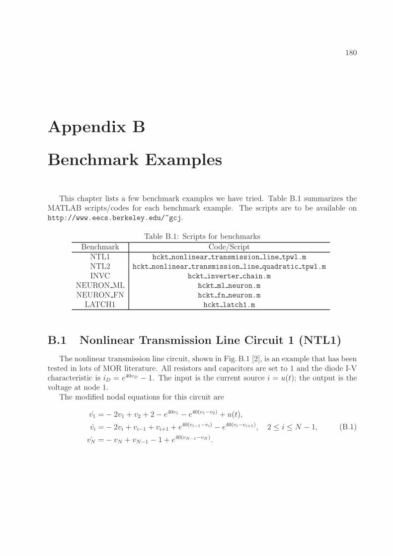
180

Appendix B

Benchmark Examples

This chapter lists a few benchmark examples we have tried. Table B.1 summarizes theMATLAB scripts/codes for each benchmark example. The scripts are to be available onhttp://www.eecs.berkeley.edu/~gcj.

Table B.1: Scripts for benchmarks

Benchmark Code/ScriptNTL1 hckt nonlinear transmission line tpwl.m

NTL2 hckt nonlinear transmission line quadratic tpwl.m

INVC hckt inverter chain.m

NEURON ML hckt ml neuron.m

NEURON FN hckt fn neuron.m

LATCH1 hckt latch1.m

B.1 Nonlinear Transmission Line Circuit 1 (NTL1)

The nonlinear transmission line circuit, shown in Fig. B.1 [2], is an example that has beentested in lots of MOR literature. All resistors and capacitors are set to 1 and the diode I-Vcharacteristic is iD = e40vD − 1. The input is the current source i = u(t); the output is thevoltage at node 1.

The modified nodal equations for this circuit are

v1 =− 2v1 + v2 + 2− e40v1 − e40(v1−v2) + u(t),

vi =− 2vi + vi−1 + vi+1 + e40(vi−1−vi) − e40(vi−vi+1), 2 ≤ i ≤ N − 1,

˙vN =− vN + vN−1 − 1 + e40(vN−1−vN ).

(B.1)

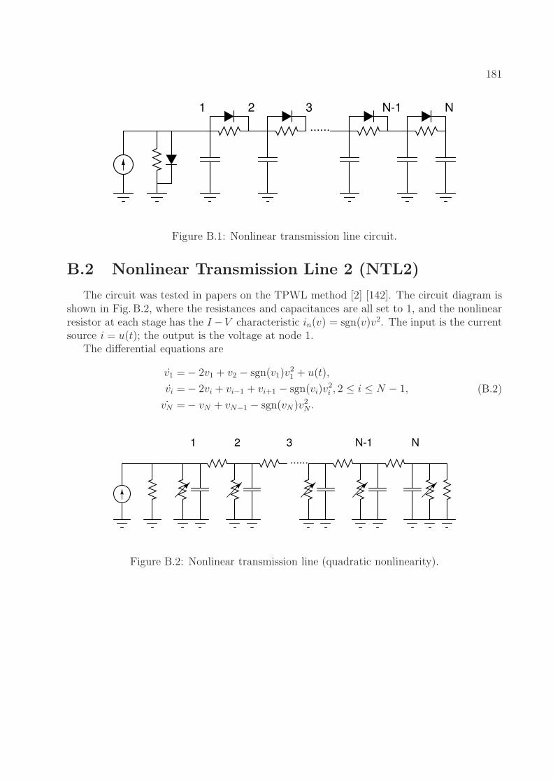
181

......

1 2 3 NN-1

Figure B.1: Nonlinear transmission line circuit.

B.2 Nonlinear Transmission Line 2 (NTL2)

The circuit was tested in papers on the TPWL method [2] [142]. The circuit diagram isshown in Fig. B.2, where the resistances and capacitances are all set to 1, and the nonlinearresistor at each stage has the I−V characteristic in(v) = sgn(v)v2. The input is the currentsource i = u(t); the output is the voltage at node 1.

The differential equations are

v1 =− 2v1 + v2 − sgn(v1)v21 + u(t),

vi =− 2vi + vi−1 + vi+1 − sgn(vi)v2i , 2 ≤ i ≤ N − 1,

˙vN =− vN + vN−1 − sgn(vN )v2N .

(B.2)

......

1 2 3 NN-1

Figure B.2: Nonlinear transmission line (quadratic nonlinearity).

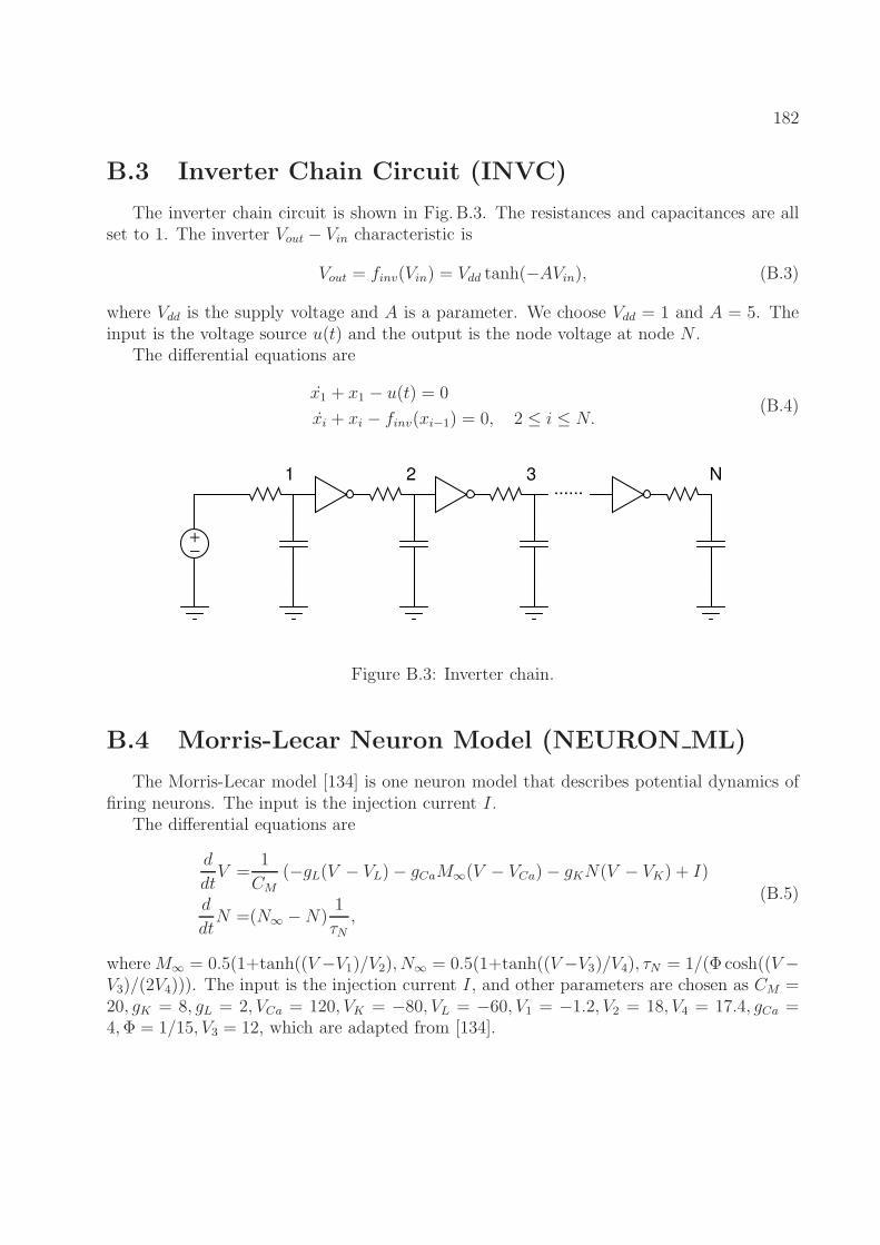
182

B.3 Inverter Chain Circuit (INVC)

The inverter chain circuit is shown in Fig. B.3. The resistances and capacitances are allset to 1. The inverter Vout − Vin characteristic is

Vout = finv(Vin) = Vdd tanh(−AVin), (B.3)

where Vdd is the supply voltage and A is a parameter. We choose Vdd = 1 and A = 5. Theinput is the voltage source u(t) and the output is the node voltage at node N .


x1 + x1 − u(t) = 0

xi + xi − finv(xi−1) = 0, 2 ≤ i ≤ N.(B.4)

......2 N

+

−

1 3

Figure B.3: Inverter chain.

B.4 Morris-Lecar Neuron Model (NEURON ML)

The Morris-Lecar model [134] is one neuron model that describes potential dynamics offiring neurons. The input is the injection current I.


d

dtV =

1

CM(−gL(V − VL)− gCaM∞(V − VCa)− gKN(V − VK) + I)

d

dtN =(N∞ −N)

1

τN,

(B.5)

whereM∞ = 0.5(1+tanh((V−V1)/V2), N∞ = 0.5(1+tanh((V−V3)/V4), τN = 1/(Φ cosh((V−V3)/(2V4))). The input is the injection current I, and other parameters are chosen as CM =20, gK = 8, gL = 2, VCa = 120, VK = −80, VL = −60, V1 = −1.2, V2 = 18, V4 = 17.4, gCa =4,Φ = 1/15, V3 = 12, which are adapted from [134].

183

B.5 FitzHugh-Nagumo Model (NEURON FN)

The FitzHugh-Nagumo model is a PDE neuron model. The input is the injection currenti0(t) which is included in the boundary condition.

Let x ∈ [0, L], t ≥ 0, the PDEs are

∂

∂tv(x, t) = ǫ

∂2

∂x2v(x, t) +

1

ǫ(f(v(x, t))− w(x, t) + c)

∂

∂tw(x, t) = bv(x, t)− γw(x, t) + c

(B.6)

withf(v) = v(v − 0.1)(1− v), (B.7)

boundary conditions∂

∂xv(0, t) = −i0(t),

∂

∂xv(L, t) = 0 (B.8)

and initial conditionsv(x, 0) = 0, w(x, 0) = 0, (B.9)

where the parameters are

L = 1, ǫ = 0.015, b = 0.5, γ = 2, c = 0.05. (B.10)

Applying finite difference on x-dimension, let

vi(t) = v(ih), wi(t) = w(ih), i = 1, · · · , N (B.11)

where h = 1/(N + 1).We obtain

∂

∂tvi(t) = ǫ

vi+1 − 2vi + vi−1

h2+

1

ǫ(f(vi(t))− wi(t) + c)) , i = 2, · · · , N − 1,

∂

∂tv1(t) = ǫ

1

h

(

v2 − v1h

+ i0(t)

)

+1

ǫ(f(v1(t))− w1(t) + c)) ,

∂

∂tvN(t) = ǫ

1

h

(

−vN − vN−1

h

)

+1

ǫ(f(vN(t))− wN(t) + c)) ,

∂

∂twi(t) = bvi(t)− γwi(t) + c, i = 1, · · · , N.

(B.12)

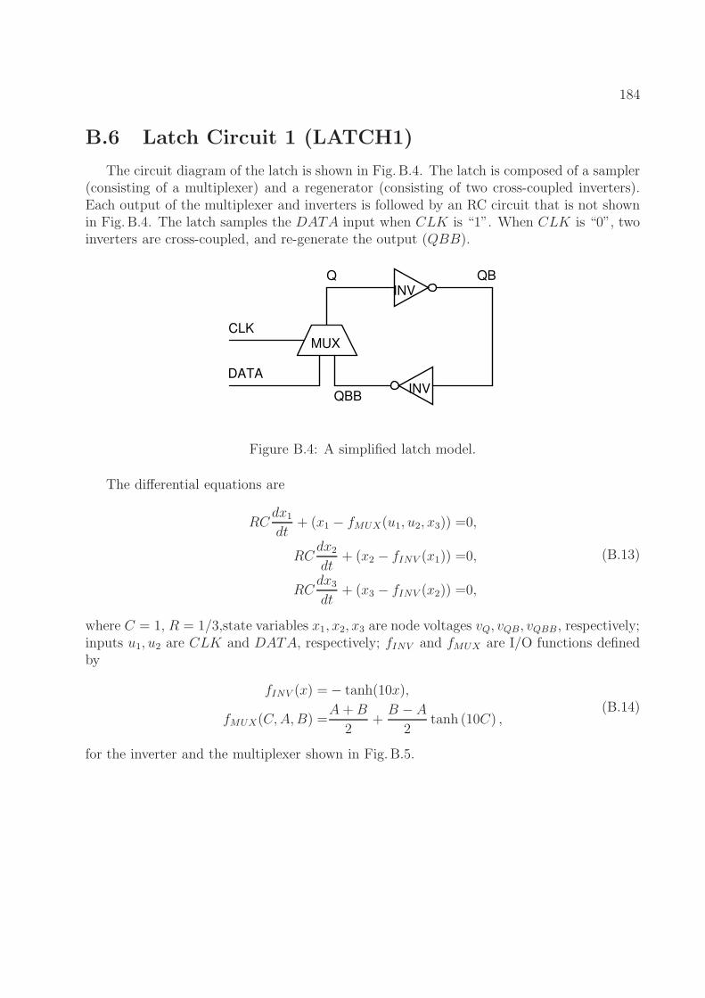
184

B.6 Latch Circuit 1 (LATCH1)

The circuit diagram of the latch is shown in Fig. B.4. The latch is composed of a sampler(consisting of a multiplexer) and a regenerator (consisting of two cross-coupled inverters).Each output of the multiplexer and inverters is followed by an RC circuit that is not shownin Fig. B.4. The latch samples the DATA input when CLK is “1”. When CLK is “0”, twoinverters are cross-coupled, and re-generate the output (QBB).

INV

INV

MUX

CLK

DATA

Q QB

QBB

Figure B.4: A simplified latch model.


RCdx1

dt+ (x1 − fMUX(u1, u2, x3)) =0,

RCdx2

dt+ (x2 − fINV (x1)) =0,

RCdx3

dt+ (x3 − fINV (x2)) =0,

(B.13)

where C = 1, R = 1/3,state variables x1, x2, x3 are node voltages vQ, vQB, vQBB, respectively;inputs u1, u2 are CLK and DATA, respectively; fINV and fMUX are I/O functions definedby

fINV (x) =− tanh(10x),

fMUX(C,A,B) =A +B

2+

B − A

2tanh (10C) ,

(B.14)

for the inverter and the multiplexer shown in Fig. B.5.

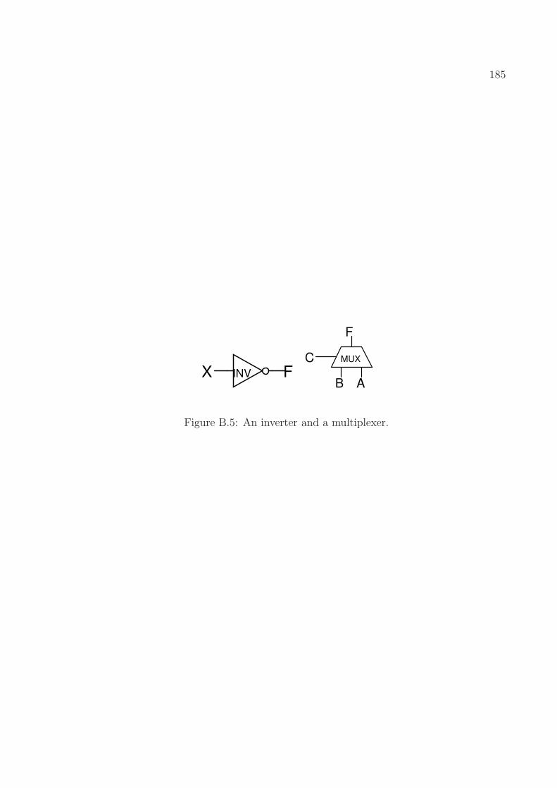
185

INVX FMUXC

B A

F

Figure B.5: An inverter and a multiplexer.

Documents

Model Order Reduction of Nonlinear Dynamical Systems · Model Order Reduction of Nonlinear Dynamical ... Model Order Reduction of Nonlinear Dynamical Systems by ... nonlinear and