Search III: Advanced Search - University of Wisconsin

CS 540 Introduction to Artificial Intelligence

Search III: Advanced Search

Fred Sala University of Wisconsin-Madison

April 15, 2021

Announcements

• Homeworks:

– HW9 in progress. All grades up to & including HW7 out.

• Class roadmap:

Tuesday, April 13 Search II

Thursday, April 15 Search III

Tuesday, April 20 Introduction to RL

Thursday, April 22 RL and Search Summary

Tuesday, April 27 AI in the Real World

Artificial In

telligence

Outline

• Advanced Search & Hill-climbing

– More difficult problems, basics, local optima, variations

• Simulated Annealing

– Basic algorithm, temperature, tradeoffs

• Genetic Algorithms

– Basics of evolution, fitness, natural selection

Search vs. Optimization

Before: wanted a path from start state to goal state

• Uninformed search, informed search

New setting: optimization

• States s have values f(s)

• Want: s with optimal value f(s) (i.e, optimize over states)

• Challenging setting: too many states for previous search approaches, but maybe not a continuous function for SGD.

Wiki TuringFin

Examples: n Queens

A classic puzzle:

• Place 8 queens on a 8 x 8 chessboard so that no two have same row, column, or diagonal.

• Can generalize to n x n chessboard.

• What are states s? Values f(s)? – State: configuration of the board

– f(s): # of conflicting queens

Wiki

Examples: TSP

Famous graph theory problem.

• Get a graph G = (V,E). Goal: a path that visits each node exactly once and returns to the initial node (a tour). – State: a particular tour (i.e., ordered list of nodes)

– f(s): total weight of the tour

(e.g., total miles traveled)

J. Yu

Examples: Satisfiability

Boolean satisfiability (e.g., 3-SAT)

• Recall our logic lecture. Conjunctive normal form

– Goal: find if satisfactory assignment exists.

– State: assignment to variables

– f(s): # satisfied clauses

(A B C) ∧ (A C D) ∧ (B D E) ∧ ( C D E) ∧ ( A C E)

Wiki

Hill Climbing

One approach to such optimization problems.

• Basic idea: move to a neighbor with a better f(s)

• Q: how do we define neighbor? – Not as obvious as our successors in search

– Problem-specific

– As we’ll see, needs a careful choice

Defining Neighbors: n Queens

In n Queens, a simple possibility:

• Look at the most-conflicting column (ties? right-most one)

• Move queen in that column vertically to a different location

…

s

f(s)=1

Neighborhood of s

f=1

f=2

Defining Neighbors: TSP

For TSP, can do something similar:

• Define neighbors by small changes

• Example: 2-change: A-E and B-F

A-B-C-D-E-F-G-H-A

A-E-D-C-B-F-G-H-A

flip

Defining Neighbors: SAT

For Boolean satisfiability,

• Define neighbors by flipping one assignment of one variable

Starting state: TFTTT

(A=F, B=F, C=T, D=T, E=T) (A=T, B=T, C=T, D=T, E=T) (A=T, B=F, C=F, D=T, E=T) (A=T, B=F, C=T, D=F, E=T) (A=T, B=F, C=T, D=T, E=F)

A B C

A C D

B D E

C D E

A C E

Hill Climbing Neighbors

Q: What’s a neighbor?

• Vague definition. For a given problem structure, neighbors are states that can be produced by a small change

• Tradeoff! – Too small? Will get struck.

– Too big? Not very efficient

• Q: how to pick a neighbor? Greedy

• Q: terminate? When no neighbor has bigger value

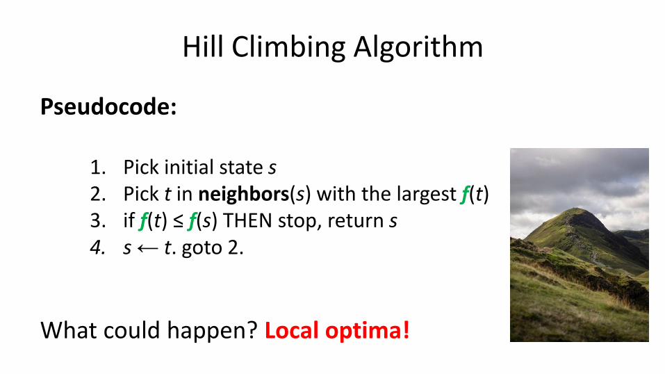
Hill Climbing Algorithm

Pseudocode:

What could happen? Local optima!

1. Pick initial state s 2. Pick t in neighbors(s) with the largest f(t) 3. if f(t) ≤ f(s) THEN stop, return s 4. s ← t. goto 2.

Hill Climbing: Local Optima

Q: Why is it called hill climbing?

L: What’s actually going on. R: What we get to see.

state

f Global optimum, where

we want to be

state

f fog

Hill Climbing: Local Optima

Note the local optima. How do we handle them?

Done?

state

f

state

f Where do I go?

Escaping Local Optima

Simple idea 1: random restarts

• Stuck: pick a random new starting point, re-run.

• Do k times, return best of the k.

Simple idea 2: reduce greed

• “Stochastic” hill climbing: randomly select between neighbors

• Probability proportional to the value of neighbors

Hill Climbing: Variations

Q: neighborhood too large?

• Generate random neighbors, one at a time. Take the better one.

Q: relax requirement to always go up?

• Often useful for harder problems

• 3SAT algorithm: Walk-SAT

D. Selsam

Break & Quiz

Q 1.1: Hill climbing and SGD are related by

(i) Both head towards optima

(ii) Both require computing a gradient

(iii) Both will find the global optimum for a convex problem

• A. (i)

• B. (i), (ii)

• C. (i), (iii)

• D. All of the above

Break & Quiz





• A. (i)

• B. (i), (ii)

• C. (i), (iii)

• D. All of the above

Break & Quiz





• A. (i) (No: (iii) also true since convexity->local optima are global)

• B. (i), (ii) (No: (ii) is false. Hill-climbing looks at neighbors only.)

• C. (i), (iii)

• D. All of the above (No: (ii) false, as above.)

Simulated Annealing

A more sophisticated optimization approach.

• Idea: move quickly at first, then slow down

• Pseudocode:

Pick initial state s For k = 0 through kmax:

T ← temperature( (k+1)/kmax ) Pick a random neighbour, t ← neighbor(s) If f(s) ≤ f(t), then s ← t Else, with prob. P(f(s), f (t), T) then s ← t

Output: the final state s

The interesting bit

Simulated Annealing: Picking Probability

How do we pick probability P? Note 3 parameters.

• Decrease with time

• Decrease with gap |f(s) - f(t)|

Pick initial state s For k = 0 through kmax:

T ← temperature( (k+1)/kmax ) Pick a random neighbour, t ← neighbor(s) If f(s) ≤ f(t), then s ← t Else, with prob. P(f(s), f (t), T) then s ← t

Output: the final state s

Simulated Annealing: Picking Probability

How do we pick probability P? Note 3 parameters.

• Decrease with time

• Decrease with gap |f(s) - f(t)|:

• Temperature cools over time. – So: high temperature, accept any t

– But, low temperature, behaves like hill-climbing

– Still, |f(s) - f(t)| plays a role: if big, replacement probability low.

Temp

tfsf |)()(|exp

Simulated Annealing: Visualization

What does it look like in practice?

Wiki

Simulated Annealing: Picking Parameters

• Have to balance the various parts., e.g., cooling schedule. – Too fast: becomes hill climbing, stuck in local optima

– Too slow: takes too long.

• Combines with variations (e.g., with random restarts) – Probably should try hill-climbing first though.

• Inspired by cooling of metals – We’ll see one more alg. inspired by nature

Break & Quiz

Q 2.1: Which of the following is likely to give the best cooling schedule for simulated annealing?

A. Tempt+1= Tempt* 1.25

B. Tempt+1= Tempt

C. Tempt+1= Tempt* 0.8

D. Tempt+1= Tempt* 0.0001

Break & Quiz


A. Tempt+1= Tempt* 1.25

B. Tempt+1= Tempt


D. Tempt+1= Tempt* 0.0001

Break & Quiz


A. Tempt+1= Tempt* 1.25 (No, temperate is increasing)

B. Tempt+1= Tempt (No, temperature is constant)


D. Tempt+1= Tempt* 0.0001 (Cools too fast---basically hill climbing)

Break & Quiz

Q 2.2: Which of the following would be better to solve with simulated annealing than A* search?

i. Finding the smallest set of vertices in a graph that involve all edges

ii. Finding the fastest way to schedule jobs with varying runtimes on machines with varying processing power

iii. Finding the fastest way through a maze

• A. (i)

• B. (ii)

• C. (i) and (ii)

• D. (ii) and (iii)

Break & Quiz


i. Finding the smallest set of vertices in a graph that involve all edges



• A. (i)

• B. (ii)

• C. (i) and (ii)

• D. (ii) and (iii)

Break & Quiz


i. Finding the smallest set of vertices in a complete graph (i.e., all nodes connected)



• A. (i) (No, (ii) better: huge number of states, don’t care about path)

• B. (ii) (No, (i) complete graph might have too many edges for A*)

• C. (i) and (ii)

• D. (ii) and (iii) (No, (iii) is good for A*: few successors, want path)

Another optimization approach based on nature

• Survival of the fittest!

Genetic Algorithms

Evolution Review

Encode genetic information in DNA (four bases)

• A/C/T/G: nucleobases acting as symbols

• Two types of changes

– Crossover: exchange between parents’ codes

– Mutation: rarer random process • Happens at individual level

Natural Selection

Competition for resources

• Organisms better fit ➔ better probability of reproducing

• Repeated process: fit become larger proportion of population

Goal: use these principles for optimization

– New terminology: state s ‘individual’

– Value f(s) is now the ‘fitness’

Genetic Algorithms Setup I

Keep around a fixed number of states/individuals

• A bit like beam search

• Call this the population

For our n Queens game example, an individual:

(3 2 7 5 2 4 1 1)

Genetic Algorithms Setup II

Goal of genetic algorithms: optimize using principles inspired by mechanism for evolution

• E.g., analogous to natural selection, cross-over, and mutation

Next generation

# of non-attacking pairs

prob. reproduction

fitness

Genetic Algorithms Pseudocode

Just one variant:

1. Let s1, …, sN be the current population 2. Let pi = f(si) / j f(sj) be the reproduction probability 3. for k = 1; k<N; k+=2

• parent1 = randomly pick according to p • parent2 = randomly pick another • randomly select a crossover point, swap strings of

parents 1, 2 to generate children t[k], t[k+1] 4. for k = 1; k<=N; k++

• Randomly mutate each position in t[k] with a small probability (mutation rate)

5. The new generation replaces the old: { s }{ t }. Repeat

Reproduction probability: pi = f(si) / j f(sj)

• Example: j f(sj) = 5+20+11+8+6=50

• p1=5/50=10%

Reproduction: Proportional Selection

Example: Scheduling Courses

Let’s run through an example:

• 5 courses: A,B,C,D,E

• 3 time slots: Mon/Wed, Tue/Thu, Fri/Sat

• Students wish to enroll in three courses

• Goal: maximize student enrollment

Courses Students

A B C 2

A B D 7

A D E 3

B C D 4

B D E 10

C D E 5


Let’s run through an example:

• State: course assignment to time slot

• Here:

– Courses A, B, E scheduled Mon/Wed

– Course D scheduled Tue/Thu

– Course C scheduled Fri/Sat

Courses Students

A B C 2

A B D 7

A D E 3

B C D 4

B D E 10

C D E 5

M M F T M

A B C D E = MMFTM


Value of a state? Say MMFTM

• Here 4+5=9 students can enroll in desired courses

Courses Students Can enroll?

A B C 2 No

A B D 7 No

A D E 3 No

B C D 4 Yes

B D E 10 No

C D E 5 Yes


First step:

• Randomly initialize and evaluate states

• Calculate reproduction probabilities

Courses Students

A B C 2

A B D 7

A D E 3

B C D 4

B D E 10

C D E 5

MMFTM = 9

TTFMM = 4

FMTTF = 19

MTTTF = 3

MMFTM = 26%

TTFMM = 11%

FMTTF = 54%

MTTTF = 9%


Next steps:

• Select parents using reproduction probabilities


• Randomly mutate new children


Continue:

• Now, get our function values for updated population


FMFTT = 11

MMTTF = 13

MMTFF = 4

FTTTF = 0

Courses Students

A B C 2

A B D 7

A D E 3

B C D 4

B D E 10

C D E 5

FMFTT = 39%

MMTTF = 46%

MMTFF = 14%

FTTTF = 0%

Variations & Concerns

Many possibilities:

• Parents survive to next generation

• Ranking instead of exact value of f(s) for reproduction probabilities

Some challenges

• State encoding

• Lack of diversity: converge too soon

• Must pick a lot of parameters

Summary

• Challenging optimization problems

– First, try hill climbing. Simplest solution

• Simulated annealing

– More sophisticated approach; helps with local optima

• Genetic algorithms

– Biology-inspired optimization routine

Acknowledgements: Adapted from materials by Jerry Zhu + Tony Gitter

(University of Wisconsin), Andrew Moore

Documents

Search III: Advanced Search - University of Wisconsin