(r|p)-Centroid Problems on Networks with Vertex and Edge

Demand†

Dominik Kress∗, Erwin Pesch

Department of Management Information Science, University of Siegen, Holderlinstraße 3, D-57068Siegen, Germany

Abstract

This paper analyzes (r|p)-centroid problems on networks with vertex and edge demandunder a binary choice rule. Bilevel programming models are presented for the discreteproblem class. Furthermore, NP-hardness proofs for the discrete and continuous (1|p)-centroid problem on general networks with edge demand only are provided. Nevertheless,an efficient algorithm to determine a discrete (1|p)-centroid of a tree network with vertexand edge demand can be derived.

Keywords: location, competitive location, centroid, edge demand, bilevel programming

1. Introduction

Location problems are concerned with the location of (physical or nonphysical) re-sources in some given space. Competitive location models (dating back to Hotelling [1])additionally incorporate the fact that location decisions have been or will be made by inde-pendent decision-makers who will subsequently compete with each other, e.g. for marketshare when we think of locating facilities such as gas stations or supermarkets. Severalreviews and classifications have appeared in this field. They include Drezner [2], Eiseltet al. [3], Eiselt and Laporte [4], Kress and Pesch [5], Plastria [6], Serra and ReVelle [7].

The representation of the location space may be divided into different classes. We fol-low ReVelle and Eiselt [8] in differentiating between d-dimensional real space and networklocation problems, each of which further being subdivided into continuous and discreteproblems. A discrete problem arises, when the set of candidate locations is assumed tobe finite and known a priori. In a continuous problem, any point of the network or thed-dimensional space is a potential location site. By identifying finite sets of points thatcapture optimal locations (finite dominating sets, Hooker et al. [9]), some continuousproblem classes can be transformed into equivalent discrete problem classes a posteriori.Customer behavior is represented by some kind of choice rule. A choice rule is said tobe binary (or deterministic), when the total demand of a customer is served by a single

∗Corresponding author, phone: +49 271 740 3402, fax: +49 271 740 2940Email addresses: dominik.kress@uni-siegen.de (Dominik Kress), erwin.pesch@uni-siegen.de

(Erwin Pesch)

† This is an Accepted Manuscript of an article published by Elsevier in Computers & OperationsResearch on 5 March 2012, available online: https://doi.org/10.1016/j.cor.2012.02.025c© 2012. This manuscript version is made available under the CC-BY-NC-ND 4.0 license http:

//creativecommons.org/licenses/by-nc-nd/4.0/

facility; it is said to be probabilistic (or proportional), if demand is split over multiple fa-cilities. Other fundamental categories of competitive location theory are related to gametheoretic aspects. Competition itself, for instance, may be static, dynamic, or competitorsmay enter in a simultaneous or sequential fashion. The latter mode of competition (rootedin the work of Hay [10] and Prescott and Visscher [11]) is characterized by two types ofplayers: leaders, who choose locations at given instants, anticipating the subsequent ac-tions of later entrants, and followers, who make their location decisions based on the pastdecisions of the leaders. The solution concept generally employed in sequential locationproblems is the Stackelberg equilibrium [12]: Assuming rational players, the location ofeach player is determined by backward induction.

Hakimi [13] formally introduced the terms (r|Xp)-medianoid problem and (r|p)-centroidproblem for sequential games with one leader (L) and one follower (F) locating p and rfacilities, respectively. Note that r and p are arbitrary input parameters. Knowing thep locations of L, denoted by Xp = (x1, ..., xp), F faces the problem of optimally locatingr facilities (with respect to some objective function): the (r|Xp)-medianoid problem. L’sproblem, the (r|p)-centroid problem, is to locate p facilities, anticipating F’s subsequentbehavior. In this paper we will consider the objective of maximizing market share forboth, L and F. We will generally precede the terms (r|p)-centroid and (r|Xp)-medianoidproblem with the terms discrete, continuous, binary or proportional throughout the restof the paper. This clarifies the type of choice rule (binary or proportional) and locationspace (discrete or continuous problems on networks) under consideration.

Whereas competitive location models in R1 typically assume the demand to be con-tinuously dispersed over the line segment, the majority of network models incorporatediscrete demand, i.e. demand arising in the vertices of the network. Dasci et al. [14]and Okunuki and Okabe [15] were among the first to consider demand densities over theedges of competitive location problems on general networks. In an urban context, themotivation is as follows: Cities are typically modeled as networks. Edges correspond tostreets and vertices represent intersections. The houses of a city are usually dispersedover the streets. Thus, demand is typically non-discrete. While Dasci et al. [14] andOkunuki and Okabe [15] consider (r|Xp)-medianoid problems, it is the aim of this paperto apply the concept of edge demand to (r|p)-centroid problems. We will show that thediscrete and continuous, binary (1|p)-centroid problem are NP-hard on general networkswith edge demand only. Furthermore, we will adapt the definition of ξ-bounding sets bySpoerhase and Wirth [16] to design an efficient algorithm to determine a discrete, binary(1|p)-centroid of a tree network with vertex and edge demand.

The remainder of this paper is organized as follows. The notation and definitions usedthroughout the paper are given in Section 2. Section 3 is devoted to the binary (r|p)-centroid problem with vertex and edge demand on general networks. We present bilevelprogramming formulations for the discrete problem class in Section 3.1. While the focusof the paper is on drawing the line between hard and easy problems, some computationalresults for the corresponding (r|Xp)-medianoid problem are given in Section 3.2 to illus-trate the need for approximate solution procedures when designing heuristic algorithmsfor the leader’s problem. The above-mentioned NP-hardness proofs are subject of Section3.3. Section 3.4 is concerned with the identification of finite dominating sets. The efficientalgorithm for the discrete, binary (1|p)-centroid problem on a tree network with vertex

2

and edge demand is given in Section 4. We introduce the basic ideas by restricting ourattention to chain networks in Section 4.1, before describing the algorithm itself in Section4.2. The paper ends with a conclusion in Section 5.

2. Basic notation and definitions

We extend and use the notation of Bandelt [17] in this paper (cf. also [18]). A networkN = (V,E, λ) consists of a finite set V (|V | = n), a finite set E (|E| = m) of two-elementsubsets of V and a mapping λ : E → R+. The pair (V,E) gives a graph in the usual sense(cf. [19]). The elements v of V are called vertices of the network. The elements e of E arethe edges. Every edge joins two distinct vertices of N . If e is an edge joining u and v thisis expressed by the shorthand e = [u, v]. We assume that all edges are undirected, hence[u, v] = [v, u]. The value λ(e) = λ(uv) is the length of e. An edge [u, u] is a loop. Thesum of the number of edges that join a vertex v ∈ V with other vertices of the networkand twice the number of loops at v is the degree of v. The points x of N (x ∈ N) are theelements of the edges (including all vertices). Two points x and y on an edge e (x, y ∈ e)determine a subedge [x, y] of e, the length of which is denoted by λ([x, y]). A path P (x, y)joining two points x ∈ [u, v] and y ∈ [w, z] is either a subedge or a sequence of edges and(at most two) subedges passing at most once through each point, where P (x, y) containsx and y but no proper connected subset of P (x, y) does. The points x and y are the endpoints of P (x, y). The length of P (x, y) is equal to the sum of the lengths of the edges andsubedges. If the length of P (x, y) is minimum among all paths connecting x and y, thenP (x, y) is a shortest path; its length is the distance d(x, y) between x and y. We defineD(p, Z) := min{d(p, z)|z ∈ Z} for a point p ∈ N and a set of points Z ⊆ N . A cycleconsists of an edge e joining two vertices u and v and some path P (u, v) 6= e connecting uand v. A network is connected if for any two points x and y there exists a path joining xand y. A connected network without cycles is a tree network. A tree network where everyvertex is incident to at most two edges is a chain network. We assume that the networksconsidered in this paper are connected and that there are no multiple edges. Moreover,we assume that there are no loops at the vertices.

Let V ′ be a subset of the vertex set of N . The network N ′ = (V ′, E ′, λ′) is thesubnetwork of N on the vertex set V ′, if E ′ is a subset of E such that each edge of Ejoining u and v belongs to E ′ if and only if u and v are in V ′. The mapping λ′ is therestriction of λ to E ′.

Let a tree network N = (V,E, λ) be rooted at some distinguished vertex r ∈ V . Foreach pair of vertices i ∈ V and j ∈ V , we call i a descendant of j, if j is on the uniquepath that connects i to the root r. If i is a descendant of j, we call j an ancestor ofi. A vertex v ∈ V is a common ancestor of two vertices x, y ∈ V , if it is an ancestorof both, x and y. A common ancestor of two vertices x, y ∈ V is the nearest commonancestor, nca(x, y), of these very vertices, if its distance to the root is the largest amongall common ancestors. If i ∈ V is a descendant of j ∈ V and [i, j] ∈ E, then i is saidto be a child of j and j is called the father of i. A vertex without children is a leaf ofthe tree network. For any vertex v ∈ V we denote the subnetwork (subtree) of N on thevertex set VTv := {v} ∪ {i ∈ V |i is a descendant of v} by Tv and the subnetwork on thevertex set V ′Tv := VTv \ {v} by T ′v.

3

We associate a (local) coordinate xuv ∈ [0, λ(uv)] with every edge [u, v] ∈ E of a graphN . Thus, we are able to define any point of the graph. The direction of counting can bedefined arbitrarily.

A finite number of users is located at the vertices of the network N (vertex demands,vertex customers). At each vertex there may be several users or none at all. Theirdemand is described by a weight function π : V → R+

0 . We define π(x) := 0 for all x /∈ V .Additionally, we consider a mapping δ : E → R+

0 with every edge e = [u, v] ∈ E. Thevalue δ(e) = δ(uv) is the uniform demand density (edge demand, edge customer) of theedge e = [u, v], i.e. the demand per unit of length (see Figure 1). δ and π may not beequal to the zero function at the same time.

uvx(uv )

(uv )

(u ) (v )

u v

Figure 1: Vertex and edge demand.

For a subnetwork N ′ of N we denote by π(V ′) the sum∑

u∈V ′ π(u) where V ′ is thevertex set of N ′. Analogously, we denote by δ(E ′) the sum

∑e∈E′ δ(e) · λ(e) where E ′

is the edge set of N ′. Finally, we define ξ(N ′) := π(V ′) + δ(E ′). We denote the ac-cumulated demand of the customers who accommodate their demand at F’s facilitiesby WF (Yr(Xp)|Xp), where Yr(Xp) corresponds to an arbitrary feasible set of F’s loca-tions, given the location decision Xp of L. The optimal follower’s market share is de-noted by W ∗

F (Yr(Xp)|Xp). Analogously, we denote L’s (optimal) market share by WL(r|p)(W ∗

L(r|p)).Let N = (V,E, λ) be a tree network. Add an artificial vertex n+ 1 with π(n+ 1) = 0

as the root of N and connect it to an arbitrary vertex s ∈ V by an artificial edge [s, n+ 1]with λ([s, n+ 1]) =∞ and δ([s, n+ 1]) = 0.

Definition 1 (Spoerhase and Wirth [16]). Let X ⊆ V \ {n + 1} be a vertex subset and0 ≤ ξ ≤ ξ(N). Set X is called ξ-bounding if

1. W ∗F (Y1(X)|X) ≤ ξ and

2. ∀ x ∈ X with father x′ we have W ∗F (Y1((X \ {x}) ∪ {x′})|(X \ {x}) ∪ {x′}) > ξ.

Finally, we define:

Definition 2. Let N = (V,E, λ) be a tree network. Furthermore, let X ⊆ V , v ∈ V andu be the father of v, {u, v} ∩ X = ∅. Then the X-subtracted subtree rooted in u is thesubnetwork on the vertex set

VXs := {u} ∪

VTv \ ⋃i∈{X∩VTv}

V ′Ti

.

4

3. The binary (r|p)-centroid problem with vertex and edge demand

In the remainder of this paper we will consider a binary choice rule, i.e. each customerchooses the closest facility to accommodate all of his demand. We additionally assumethat ties are broken in favor of the leader. This is a common assumption in the fieldof competitive location problems; see, for example, Hakimi [20] (binary (r|p)-centroidproblem with vertex demand only) or Hansen and Labbe [21], Hansen and Thisse [22](Condorcet and Simpson points). As a direct consequence we may assume that p+ r ≤ nfor the discrete version of the centroid problem under consideration.

3.1. Bilevel programming models for the discrete, binary (r|p)-centroid problem with vertexand edge demand

Consider the discrete, binary (r|p)-centroid problem with vertex and edge demand.For the remainder of this section, we assume – without loss of generality – that theunderlying network is complete. If this is not the case, we simply add missing edges withinfinite edge lengths and zero demand densities.

We define the following variables:

xFij :=

1 if the vertex customers located in vertex i are served

by a follower’s facility located in vertex j,0 else,

∀ i, j ∈ V, (1)

xLij :=

1 if the vertex customers located in vertex i are served

by a leader’s facility located in vertex j,0 else,

∀ i, j ∈ V, (2)

yFj :=

{1 if the follower locates in vertex j,0 else,

∀ j ∈ V, (3)

yLj :=

{1 if the leader locates in vertex j,0 else,

∀ j ∈ V. (4)

For all i, j = 1, ..., n, let Cij and Cij be the sets of vertices k with d(k, i) < d(i, j) ord(k, i) = d(i, j), respectively (cf. also Dobson and Karmarkar [23]). Furthermore, defineCij := Cij∪Cij. We can now state a binary bilevel nonlinear programming model (BBNP)for the problem under consideration (refer to Dempe [24] for an introduction to bilevelprogramming).

maxxL,yL

n∑i=1

n∑j=1

xLij

[π(i) +

n∑k=1

12δ(i, k)

(λ(i, k)− d(i, j) +

n∑l=1

(xLkl + xFkl)d(k, l)

)](5)

subject ton∑j=1

yLj = p, (6)

xLij ≤ yLj ∀ i, j = 1, ..., n, (7)n∑j=1

xLij ≤ 1 ∀ i = 1, ..., n, (8)

xLij + yLk ≤ 1 ∀ i, j = 1, ..., n, k ∈ Cij (9)

xLij + yFk ≤ 1 ∀ i, j = 1, ..., n, k ∈ Cij (10)

5

and xF , yF being a solution of

maxxF ,yF

n∑i=1

n∑j=1

xFij

[π(i) +

n∑k=1

12δ(i, k) (λ(i, k)− d(i, j)

+n∑l=1

(xLkl + xFkl)d(k, l))

](11)

subject ton∑j=1

yFj = r, (12)

xFij ≤ yFj ∀ i, j = 1, ..., n, (13)n∑j=1

(xFij + xLij

)= 1 ∀ i = 1, ..., n, (14)

xFij + yLk ≤ 1 ∀ i, j = 1, ..., n, k ∈ Cij (15)

xFij + yFk ≤ 1 ∀ i, j = 1, ..., n, k ∈ Cij (16)

xLij, xFij ∈ {0, 1} ∀ i, j = 1, ..., n, (17)

yLj , yFj ∈ {0, 1} ∀ j = 1, ..., n. (18)

The objective functions (5) and (11) correspond to the maximization of the marketshare of each of the players, taking into account vertex and edge demand. Constraints (6)and (12) ensure that the players locate exactly p and r facilities, respectively. Conditions(7) and (13) guarantee that a (vertex) customer can only be served if the correspondingfacility has been opened. Constraints (8) and (14) relate to the fact that the demand ofeach (vertex) customer must be served by exactly one facility, while conditions (9), (10),(15) and (16) guarantee that each (vertex) customer is served by its closest facility (cf.Dobson and Karmarkar [23]). Observe that edge customers are guaranteed to be servedimplicitly. Figure 2 depicts an example. Vertex i is served by a leader’s facility in vertexj, while vertex k is served by a follower’s facility in vertex l. Therefore, there must exist apoint xik = x on edge [i, k], where d(i, j) + x = λ(i, k)− x+ d(k, l). Every edge customerlocated at xik ≤ x (xik > x) will be served by the leader (follower).

([ i ,k ]),

([ i ,k ])

i kj l

ikx

d( j ,i ) d(k,l )

L

ijx 1 F

klx 1

Figure 2: Serving of edge customers.

Observe that

n∑i=1

n∑j=1

xLij

[π(i) +

n∑k=1

1

2δ(i, k)

(λ(i, k)− d(i, j) +

n∑l=1

(xLkl + xFkl)d(k, l)

)]

=n∑i=1

n∑j=1

xLijπ(i) +n∑i=1

n∑j=1

n∑k=1

1

2δ(i, k)xLij (λ(i, k)− d(i, j))

+

n∑i=1

n∑j=1

n∑k=1

n∑l=1

1

2δ(i, k)xLijx

Lkld(k, l) +

n∑i=1

n∑j=1

n∑k=1

n∑l=1

1

2δ(i, k)xLijx

Fkld(k, l).

6

An analogous result holds for the follower’s objective function. Thus, we may linearizeBBNP by defining binary variables zLLijkl, z

LFijkl, z

FLijkl and zFFijkl for all i, j, k, l = 1, ..., n and

introducing additional constraints. This results in a binary bilevel linear programmingmodel (BBLP).

maxxL,yL

n∑i=1

n∑j=1

xLijπ(i) +n∑i=1

n∑j=1

n∑k=1

12δ(i, k)xLij (λ(i, k)− d(i, j))

+n∑i=1

n∑j=1

n∑k=1

n∑l=1

12δ(i, k)zLLijkld(k, l) +

n∑i=1

n∑j=1

n∑k=1

n∑l=1

12δ(i, k)zLFijkld(k, l) (19)

subject to constraints (6)-(10)

zLLijkl ≤ 12(xLij + xLkl) ∀ i, j, k, l = 1, ..., n, (20)

zLFijkl ≤ 12(xLij + xFkl) ∀ i, j, k, l = 1, ..., n, (21)

and xF , yF being a solution of

maxxF ,yF

n∑i=1

n∑j=1

xFijπ(i) +n∑i=1

n∑j=1

n∑k=1

12δ(i, k)xFij (λ(i, k)− d(i, j))

+n∑i=1

n∑j=1

n∑k=1

n∑l=1

12δ(i, k)zFLijkld(k, l)

+n∑i=1

n∑j=1

n∑k=1

n∑l=1

12δ(i, k)zFFijkld(k, l) (22)

subject to constraints (12)-(18)

zFLijkl ≤ 12(xFij + xLkl) ∀ i, j, k, l = 1, ..., n, (23)

zFFijkl ≤ 12(xFij + xFkl) ∀ i, j, k, l = 1, ..., n, (24)

zLLijkl, zLFijkl ∈ {0, 1} ∀ i, j, k, l = 1, ..., n, (25)

zFLijkl, zFFijkl ∈ {0, 1} ∀ i, j, k, l = 1, ..., n. (26)

Constraints (20), (21), (23) and (24) can easily be rearranged to receive a disaggregatedmodel (BBLP2). Inequalities (20), for example, may be replaced by

zLLijkl ≤ xLij ∀ i, j, k, l = 1, ..., n, (27)

zLLijkl ≤ xLkl ∀ i, j, k, l = 1, ..., n. (28)

3.2. Potential solution approaches for the discrete, binary (r|p)-centroid problem on gen-eral networks with vertex and edge demand

The focus in the remainder of this paper is on drawing the line between hard and easy(r|p)-centroid problems with vertex and edge demand. Nevertheless, we give some basicresults concerning the design of solution approaches for the discrete, binary (r|p)-centroidproblem on general networks with vertex and edge demand in this section.

Due to their hierarchical structure, bilevel programming problems are very hard tosolve. The fact that even the linear bilevel programming problem in continuous variablesis NP-hard in the strong sense [25, Chap. 5] suggests, that we are unlikely to be confrontedwith polynomially time solvable problems. Indeed, as we will see in the following section,the discrete, binary (1|p)-centroid problem on a general network is NP-hard if we consider

7

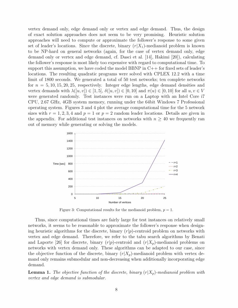
vertex demand only, edge demand only or vertex and edge demand. Thus, the designof exact solution approaches does not seem to be very promising. Heuristic solutionapproaches will need to compute or approximate the follower’s response to some givenset of leader’s locations. Since the discrete, binary (r|X1)-medianoid problem is knownto be NP-hard on general networks (again, for the case of vertex demand only, edgedemand only or vertex and edge demand, cf. Dasci et al. [14], Hakimi [20]), calculatingthe follower’s response is most likely too expensive with regard to computational time. Tosupport this assumption, we have coded the model BBNP in C++ for fixed sets of leader’slocations. The resulting quadratic programs were solved with CPLEX 12.2 with a timelimit of 1800 seconds. We generated a total of 50 test networks; ten complete networksfor n = 5, 10, 15, 20, 25, respectively. Integer edge lengths, edge demand densities andvertex demands with λ([u, v]) ∈ [1, 5], δ([u, v]) ∈ [0, 10] and π(u) ∈ [0, 10] for all u, v ∈ Vwere generated randomly. Test instances were run on a Laptop with an Intel Core i7CPU, 2.67 GHz, 4GB system memory, running under the 64bit Windows 7 Professionaloperating system. Figures 3 and 4 plot the average computational time for the 5 networksizes with r = 1, 2, 3, 4 and p = 1 or p = 2 random leader locations. Details are given inthe appendix. For additional test instances on networks with n ≥ 40 we frequently ranout of memory while generating or solving the models.

600

800

1000

1200

1400

1600

Time [sec] r=1

r=2

r=3

0

200

400

5 10 15 20 25

Number of vertices

r=4

Figure 3: Computational results for the medianoid problem, p = 1.

Thus, since computational times are fairly large for test instances on relatively smallnetworks, it seems to be reasonable to approximate the follower’s response when design-ing heuristic algorithms for the discrete, binary (r|p)-centroid problem on networks withvertex and edge demand. Therefore, we refer to the tabu search algorithms by Benatiand Laporte [26] for discrete, binary (r|p)-centroid and (r|Xp)-medianoid problems onnetworks with vertex demand only. These algorithms can be adapted to our case, sincethe objective function of the discrete, binary (r|Xp)-medianoid problem with vertex de-mand only remains submodular and non-decreasing when additionally incorporating edgedemand.

Lemma 1. The objective function of the discrete, binary (r|Xp)-medianoid problem withvertex and edge demand is submodular.

8

100

150

Time [sec] r=1

r=2

r=3

0

50

5 10 15 20 25

Number of vertices

r=4

Figure 4: Computational results for the medianoid problem, p = 2.

Proof. Let Yr be a solution to a discrete, binary (r|Xp)-medianoid problem with vertexand edge demand. Furthermore, let S ⊂ T ⊂ Yr and k ∈ V \T . We want to show thatWF (T ∪ {k}|Xp)−WF (T |Xp) ≤ WF (S ∪ {k}|Xp)−WF (S|Xp).

We define ∆v(T, k) (∆v(S, k)) to be the increase in the follower’s market share that isinduced by vertex customer v ∈ V when augmenting T (S) with an additional facility invertex k. Similarly, ∆[u,v](T, k) (∆[u,v](S, k)) is defined to be the increase in the follower’smarket share that is induced by the demand over edge [u, v]. Therefore, WF (T∪{k}|Xp)−WF (T |Xp) =

∑v∈V ∆v(T, k) +

∑[u,v]∈E ∆[u,v](T, k) and WF (S ∪ {k}|Xp) −WF (S|Xp) =∑

v∈V ∆v(S, k) +∑

[u,v]∈E ∆[u,v](S, k).One of the following cases holds for every vertex v ∈ V :

1. D(v, T ) ≥ D(v,Xp)

(a) and d(v, k) ≥ D(v,Xp),

(b) and d(v, k) < D(v,Xp),

2. D(v, T ) < D(v,Xp), D(v, S) ≥ D(v,Xp)

(a) and d(v, k) ≥ D(v,Xp),

(b) and d(v, k) < D(v,Xp), d(v, k) ≥ D(v, T ),

(c) and d(v, k) < D(v,Xp), d(v, k) < D(v, T ),

3. D(v, S) < D(v,Xp)

(a) and d(v, k) ≥ D(v, S),

(b) and d(v, k) < D(v, S), D(v, S) = D(v, T ),

(c) and d(v, k) < D(v, S), D(v, S) > D(v, T ).

Thus, for an arbitrary vertex v ∈ V , we have ∆v(S, k) = ∆v(T, k) = 0 for cases1.a, 2.a, 3.a, 3.b and 3.c; ∆v(S, k) = ∆v(T, k) = π(v) for case 1.b; ∆v(S, k) = π(v) ≥

9

∆v(T, k) = 0 for cases 2.b and 2.c. Similarly, for an arbitrary edge [u, v] ∈ E, we have∆[u,v](T, k) ≤ ∆[u,v](S, k). The related case differentiation is fairly simple but ratherlengthy (36 possible combinations of cases 1.a – 3.c). Hence, for the sake of brevity, weleave it to the reader.

Obviously, if S ⊂ T , then WF (S|Xp) ≤ WF (T |Xp). This is a direct consequence ofthe non-negativity of the vertex demands and edge demand densities. Hence, analogouslyto Benati and Laporte [26], one may apply Theorem 9.3 of Nemhauser and Wolsey [27,Chap. III.3]. Therefore, W ∗

F (r|Xp) ≤ (1 − [(r − 1)/r]r)−1W gF (r|Xp), where W g

F (r|Xp) isthe follower’s market share obtained through a greedy heuristic.

Another promising approach might be the use of genetic algorithms, as the study byJaramillo et al. [28] indicates (cf. also Arostegui Jr. et al. [29]).

3.3. Some complexity results

This section aims at extending some well known complexity results on (r|p)-centroidproblems. Hakimi [20] provides a NP-hardness proof for the continuous, binary (1|p)-centroid problem on a general network with vertex demand only. Spoerhase and Wirth[16] have recently extended this result by showing that Hakimi’s result remains trueon pathwidth bounded graphs with vertex demand only.1 Hence, we can immediatelyconclude:

Theorem 1. The problem of finding a continuous, binary (1|p)-centroid of a networkN = (V,E, λ) with vertex and edge demand is NP-hard.

Proof. The NP-hard [20] continuous, binary (1|p)-centroid problem with vertex demandonly is a special case of the continuous, binary (1|p)-centroid problem with vertex andedge demand.

In what follows, we will show that the problem remains NP-hard even if we drop thevertex weights. This is in line with the results of Dasci et al. [14] for the continuous,binary (r|X1)-medianoid problem with (vertex and) edge demand.

Theorem 2. The problem of finding a continuous, binary (1|p)-centroid of a networkN = (V,E, λ) with edge demand only, i.e. π(v) = 0 for all v ∈ V , is NP-hard.

Proof. The proof is in analogy to Hakimi [20] who considers networks with vertex demandonly. The theorem is proven by reducing the Vertex Cover (VC) problem (cf. Garey andJohnson [30, p. 190]).

Vertex Cover Problem: Given a graph G = (V,E) and an integer p ≤ |V |, is there asubset V ′ ⊆ V with |V ′| ≤ p such that for each edge e = [u, v] ∈ E at least one of u andv belongs to V ′?

Consider an instance I(V C) of the VC problem on graph G = (V,E) and replace eachedge ej = [u, v] ∈ E by the structure shown in Figure 5 (“diamond structure joining uand v” (Hakimi [20])) to construct a network N1 = (V1, E1) with the corresponding edgelengths λ and edge demand densities δ.

1See Spoerhase and Wirth [16] for a definition of pathwidth bounded graphs.

10

u v

(0,2)(0,2

)

(0,2)

(

0,2)

'''

je

''''

je Legend:

a b( ([ a,b]), ([ a,b]))

''

je

(0,1) (0,1)

(0,1)(0,1)

(0,1)

(0,1)

(1,1)

'

je

Figure 5: Diamond structure.

We will show that there exists a set of p points Xp on N1 such that WF (Y1(Xp)|Xp) ≤ 1for every point Y1(Xp) on N1 if and only if the VC instance has a solution. This will provethe theorem.

“If”: Suppose V ′ is a solution of I(V C) and let Xp = V ′ on N1. Then for any diamondstructure joining u and v in N1, either u, v or both belong to V ′ = Xp. Thus, we obviouslyhave WF (Y1(Xp)|Xp) ≤ 1 for any point Y1(Xp) on N1 (recall that ties are broken in favorof the leader).

“Only if”: Assume that a set of p points Xp on N1 is such that WF (Y1(Xp)|Xp) ≤ 1for every point Y1(Xp) on N1. If there exists at least one point of Xp on each diamondof N1, then one can move these points to (≤ p) vertices V ′ ⊆ V such that each diamondhas at least one vertex in V ′. Then V ′ is a solution to I(V C). Therefore, we mayassume that there exists a diamond structure in N1 joining, say, u and v such that thisdiamond structure contains no point of Xp. Suppose, min{D(u,Xp), D(v,Xp)} > 2. It isimmediately implied that WF (u|Xp) ≥ 2 or WF (v|Xp) ≥ 2 so that we may assume 0 <min{D(u,Xp), D(v,Xp)} ≤ 2. Without loss of generality, let min{D(u,Xp), D(v,Xp)} =D(u,Xp). Let us say there exists another diamond in N1 that corresponds to edge e =[u, v′] ∈ E and thus joins u and v′, where v 6= v′. If there is exactly one point xp ∈ Xp onthis diamond, then we can always select Y1(Xp) to lie on an edge of this diamond incidentto u such that WF (Y1(Xp)|Xp) > 1:

1. If xp is a point on edge [u, e′′′′

] (or, analogously, on edge [u, e′]) with 0 < d(u, xp) < 2,

then we select Y1(Xp) = u.

2. If xp is a point on edge [u, e′′′

] (or, analogously, on edge [u, e′′]) with 0 < d(u, xp) < 1,

then we choose Y1(Xp) = u as well.

3. If xp is a point on edge [v′, e′′′

] or [e′′′, e′′′′

] (including the vertices v′, e′′′

and e′′′′

),then we select Y1(Xp) to lie on edge [u, e

′′] such that d(u, Y1(Xp)) < D(v,Xp). The

case where xp is a point on edge [v′, e′′] or [e

′, e′′] is treated analogously (symmetry

of the diamond).

4. If xp is a point on edge [e′′, e′′′

] with xp 6= e′′

and xp 6= e′′′

, then we select Y1(Xp) = e′′

or Y1(Xp) = e′′′

.

11

Therefore, there must exist at least two points of Xp on the diamond structure joining uand v′. This implies that, if there exist no points of Xp on an arbitrary diamond structureof N1, then there are at least two points of Xp on one “adjacent” diamond structure ofN1. Therefore, there are enough points to be moved to all diamonds of N1 so that theexistence of a solution to VC is established.

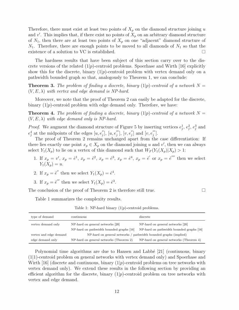
The hardness results that have been subject of this section carry over to the dis-crete versions of the related (1|p)-centroid problems. Spoerhase and Wirth [16] explicitlyshow this for the discrete, binary (1|p)-centroid problem with vertex demand only on apathwidth bounded graph so that, analogously to Theorem 1, we can conclude:

Theorem 3. The problem of finding a discrete, binary (1|p)-centroid of a network N =(V,E, λ) with vertex and edge demand is NP-hard.

Moreover, we note that the proof of Theorem 2 can easily be adapted for the discrete,binary (1|p)-centroid problem with edge demand only. Therefore, we have:

Theorem 4. The problem of finding a discrete, binary (1|p)-centroid of a network N =(V,E, λ) with edge demand only is NP-hard.

Proof. We augment the diamond structure of Figure 5 by inserting vertices e1j , e2j , e

3j and

e4j at the midpoints of the edges [u, e′′j ], [u, e

′′′j ], [v, e

′′j ] and [v, e

′′′j ].

The proof of Theorem 2 remains unchanged apart from the case differentiation: Ifthere lies exactly one point xp ∈ Xp on the diamond joining u and v′, then we can alwaysselect Y1(Xp) to lie on a vertex of this diamond such that WF (Y1(Xp)|Xp) > 1:

1. If xp = v′, xp = e1, xp = e2, xp = e3, xp = e4, xp = e′

or xp = e′′′′

then we selectY1(Xp) = u.

2. If xp = e′′

then we select Y1(Xp) = e4.

3. If xp = e′′′

then we select Y1(Xp) = e3.

The conclusion of the proof of Theorem 2 is therefore still true.

Table 1 summarizes the complexity results.

Table 1: NP-hard binary (1|p)-centroid problems.

type of demand continuous discrete

vertex demand only NP-hard on general networks [20] NP-hard on general networks [20]

NP-hard on pathwidth bounded graphs [16] NP-hard on pathwidth bounded graphs [16]

vertex and edge demand NP-hard on general networks / pathwidth bounded graphs (implied)

edge demand only NP-hard on general networks (Theorem 2) NP-hard on general networks (Theorem 4)

Polynomial time algorithms are due to Hansen and Labbe [21] (continuous, binary(1|1)-centroid problem on general networks with vertex demand only) and Spoerhase andWirth [16] (discrete and continuous, binary (1|p)-centroid problems on tree networks withvertex demand only). We extend these results in the following section by providing anefficient algorithm for the discrete, binary (1|p)-centroid problem on tree networks withvertex and edge demand.

12

3.4. Finite dominating sets

A finite dominating set for the continuous, binary (r|Xp)-medianoid problem withvertex demand only has been introduced by Megiddo et al. [31]. The authors prove thatthere always exists an optimal solution at a set of so called boundary points (cardinalityO(nm)) of the network. Dasci et al. [14] extend this result to the case of vertex and edgedemand. They show that an instance of the continuous, binary (r|Xp)-medianoid problemwith vertex and edge demand does not always possess an optimal solution. Therefore,they seek ε-optimal solutions, i.e. solutions that guarantee an objective function value atmost ε units away from a known upper bound, and establish a finite dominating set ofcardinality O(nm) by presenting a simple augmentation of the boundary point set. Oneneeds to additionally consider the set of all γ-points, i.e. points located γ units away froma vertex, where γ has to be sufficiently small.

Discretization results concerning (r|p)-centroid problems are rather limited in the lit-erature (cf. Kress and Pesch [5]). An optimal solution to the continuous, binary (r|1)-centroid problem of a general network with vertex demand only is always a vertex forr ≥ 2, while this is not the case for r = 1. If we restrict the network to be a tree, however,there always exists a vertex that is a (1|1)-centroid (see Hakimi [20] and the referencestherein). It is easy to see that the former result carries over to the case of vertex andedge demand, while the latter does not, i.e. there exist tree networks with vertex andedge demand without a (1|1)-centroid located in a vertex. Consider, for example, Figure1 with π(u) = π(v) = 0 and λ(uv) = δ(uv) = 1.

Proposition 1. Let r ≥ 2. Then there always exists a vertex v ∈ V that is an optimalsolution to the continuous, binary (r|1)-centroid problem with vertex and edge demand,defined on a network N = (V,E, λ).

The proof is straight forward. Assume that the leader locates in an arbitrary pointx /∈ V of the network. Then there exists an (ε-) optimal solution to the correspondingmedianoid problem with two follower’s facilities located infinitesimally close to x suchthat the leader’s gain is (arbitrarily close to) 0. Locating the leader’s facility in a vertexv ∈ V , in contrast, will enforce the corresponding vertex customers to accommodate theirdemand at the leader’s facility.

Spoerhase and Wirth [16] derive a finite dominating set for the continuous, binary(1|p)-centroid problem on tree networks with vertex demand only. They restrict λ :E → Q+ and π : V → Q+

0 . Thus, they may assume without loss of generality thatthe edge lengths and vertex demands are integer numbers (cf. Section 4). The authorsshow that there always exists an optimal solution to the leader’s problem, such that thedistance from any of the leader’s facilities to any vertex is an integer number or an integernumber divided by two. Note that this discretization result is not polynomial. While, asdescribed above, Dasci et al. [14] are able to show that the discretization result by Megiddoet al. [31] almost directly applies when additionally considering edge demand, the same isimplausible for the finite dominating set just described for the continuous, binary (1|p)-centroid problem on tree networks. Consider, for instance, a chain network N = (V,E, λ)with V = {1, 2, 3}, E = {[1, 2], [2, 3]}, δ([1, 2]) = 1, δ([2, 3]) = 2, λ([1, 2]) = λ([2, 3]) = 1and π(1) = π(2) = π(3) = 0. It is easy to see that the unique (1|1)-centroid x is locatedon edge [2, 3] with d(1, x) = 1.25. Moreover, Spoerhase and Wirth [16] show that, on a

13

chain network, the continuous version of the binary (r|p)-centroid problem with vertexdemand only is NP-hard, while the discrete version is not. Hence, they conjecture thata polynomial finite dominating set is unlikely to exist for the continuous, binary (r|p)-centroid problem on general networks with vertex demand only. This holds for the caseof vertex and edge demand as well. Hence, we leave the question of whether or not thereexists a more general discretization result than the one given in Proposition 1 for futureresearch and turn our attention to the discrete problem class.

4. An algorithm for the discrete, binary (1|p)-centroid problem on tree net-works with vertex and edge demand

Before describing the algorithm itself in Section 4.2, we will introduce the basic ideasby restricting our attention to chain networks in Section 4.1. We impose an additionalassumption on the networks under consideration, i.e. we assume λ : E → Q+, δ : E → Q+

0

and π : V → Q+0 . As a direct consequence, we may assume without loss of generality

that the edge lengths, demand densities and vertex demands are integer numbers forthe remainder of this paper: Let all edge lengths, demand densities and vertex demandsbe expressed as fractions of two integers and define c to be the least common multipleof their denominators. Then we can transform N into a network N ′ = (V,E, λ′) withλ′(uv) = cλ(uv), δ′(uv) = cδ(uv) for all [u, v] ∈ E and π′(u) = c2π(u) for all u ∈ Vwithout changing the ratio of the market shares of leader and follower for any feasiblelocation setting.

4.1. Chain networks

Consider a chain network N = (V,E, λ) with vertex set V = {u1, ..., un} and edgeset E = {[ui, ui+1]|i = 1, ..., n − 1} (see Figure 6). Global variables x and t allow thedefinition of any point of the chain network. For the sake of notational convenience, wewill denote the vertices by natural numbers, i.e. i instead of ui, whenever possible. Thedistinction of vertex numbers and distinct values of the global variables x and t will, ingeneral, become clear from the context.

1 2

1 2

([ u ,u ]),

([ u ,u ])

u1 u2 ui ui+1 un-1 un

1(u ) 2(u ) i(u ) i 1(u ) n 1(u ) n(u )

x,t

i i 1

i i 1

([ u ,u ]),

([ u ,u ])

n 1 n

n 1 n

([ u ,u ]),

([ u ,u ])

Figure 6: Chain network.

We define

f(x) :=∑

i∈V,d(1,i)<x

π(i) +

x∫0

δ(t)dt, (29)

where δ(t) := 0 for all t < 0 and t > d(1, n).

14

This results in

f(x) =

0 if x ≤ 0,

π(1) + δ([1, 2])x if 0 < x ≤ d(1, 2),...

...u−2∑i=1

[δ([i, i+ 1])λ([i, i+ 1]) + π(i)]

+ π(u− 1) + δ([u− 1, u])(x− d(1, u− 1))

if d(1, u− 1) < x ≤ d(1, u),

......

n−2∑i=1

[δ([i, i+ 1])λ([i, i+ 1]) + π(i)]

+ π(n− 1) + δ([n− 1, n])(x− d(1, n− 1))

if d(1, n− 1) < x ≤ d(1, n),

n−1∑i=1

[δ([i, i+ 1])λ([i, i+ 1]) + π(i)] + π(n) if x > d(1, n).

(30)

Note that, after applying a simple preprocessing procedure of linear time complexity,one can evaluate f(x) in constant time for any x. Figure 7 gives an example.

f(x)

30

15

3 4 5 6

(1) 4

([1,2 ]) 1,

([1,2 ]) 2

1 2

(6 ) 2 (5 ) 1 (4 ) 3 (3 ) 2 (2 ) 1

([ 2,3 ]) 2,

([ 2,3 ]) 1

([ 3,4 ]) 2,

([ 3,4 ]) 3

([ 4,5 ]) 1,

([ 4,5 ]) 1

([ 5,6 ]) 3,

([ 5,6 ]) 2

x

Figure 7: Function f(x).

Let the leader’s locations be the vertices j and k with j ≤ k and let the follower’slocation be vertex i 6= j, k. Then we can easily determine an open interval ]a, b[ witha < b and a, b ∈ [0, d(1, n)] of customers, who accommodate their demand at the follower’sfacility:

a =

0 if i < j,12(d(1, j) + d(1, i)) if j < i < k,

12(d(1, k) + d(1, i)) if i > k,

(31)

15

b =

12(d(1, j) + d(1, i)) if i < j,

12(d(1, k) + d(1, i)) if j < i < k,

d(1, n) if i > k.

(32)

The customers located at a and b have to be considered separately, so that the follower’smarket share can be calculated as follows:

WF (i|j, k) =

f(b)− f(a) if i < j,

f(b)− f(a)− π(a) if j < i < k,

f(b)− f(a)− π(a) + π(n) if i > k.

(33)

Thus, we can state:

Lemma 2. The problem of finding a discrete, binary (1|X2)-medianoid of a chain networkN = (V,E, λ) with vertex and edge demand can be solved in linear time O(n).

Proof. An algorithm is as follows. It determines (not necessarily all) (1|X2)-medianoids,stored in Y , as well as the corresponding market share of the follower, ξ∗s .

Algorithm 4.1 discrete, binary (1|X2)-medianoid of chain network with vertex and edgedemand

1: Y := ∅2: ξs := 0, ξ∗s := 03: for i = j − 1 to k + 1, i 6= j, i 6= k, i 6= 0, i 6= n+ 1 do4: ξs = WF (i|j, k) (Equations (31)-(33))5: if ξs > ξ∗s then6: Y = {i}7: ξ∗s = ξs8: else if ξs = ξ∗s then9: Y = Y ∪ {i}

10: end if11: end for12: if Y = ∅ then13: Y = Y ∪ {1}14: end if

We are now able to derive an efficient algorithm for the centroid problem by combiningAlgorithm 4.1 and the definition of ξ-bounding sets, presented by Spoerhase and Wirth[16] for the case of vertex demand only (see section 2). To this end we add an artificialvertex n+ 1 with π(n+ 1) = 0 and an artificial edge [n, n+ 1] with λ([n, n+ 1]) =∞ andδ([n, n+ 1]) = 0 to the chain network.

Lemma 3. Let 0 < p ≤ n with p ∈ N and 0 ≤ ξ ≤ ξ(N) with ξ ∈ R. If, for a chainnetwork N = (V,E, λ) with vertex and edge demand, there exists a ξ-bounding set with atmost p elements, we can determine one such set (or decide that there is no such set) inO(n2) time.

16

Proof. Observe that the cases ξ = 0 and ξ = ξ(N) are trivial, i.e. we can easily decideif a ξ-bounding set exists and if so, it is a simple matter to find such a set. Hence, weassume 0 < ξ < ξ(N) in the following.

Algorithm 4.2 determines a set X of at most p elements that form a ξ-bounding set inthe proposed running time. If there is no such set, the algorithm terminates with X = ∅.

Algorithm 4.2 ξ-bounding set X with |X| ≤ p of chain network with vertex and edgedemand

1: X := ∅2: ξs := π(1) + 1

2δ([1, 2])λ([1, 2])

3: i := 24: while ξs ≤ ξ and i ≤ n− 1 do5: i = i+ 16: ξs = ξs + 1

2δ([i− 2, i− 1])λ([i− 2, i− 1]) + π(i− 1) + 1

2δ([i− 1, i])λ([i− 1, i])

7: end while8: if i = n and ξs ≤ ξ then9: X := X ∪ {i}

10: else11: X = X ∪ {i− 1}12: end if13: while |X| ≤ p and i ≤ n do14: ξs = 015: while ξs ≤ ξ and i ≤ n do16: i = i+ 117: Call Algorithm 4.1 on subnetwork N ′ with vertex set V ′ = {max{l|l ∈ X}, ..., i}

and j = max{l|l ∈ X}, k = i. It results in ξ∗s and a set Y .18: ξs = ξ∗s19: end while20: if ξs > ξ then21: X = X ∪ {i− 1}22: end if23: end while24: if |X| = p+ 1 then25: X := ∅26: end if

Obviously, the set of all (1|p)-centroids of a chain network with follower gain ξ containsall ξ-bounding sets with at most p elements. Thus, we may state the main result of thissection:

Theorem 5. The problem of finding a discrete, binary (1|p)-centroid of a chain net-work N = (V,E, λ) with vertex and edge demand can be solved with time complexityO(n2 log ξ(N)).

17

Proof. We apply bisection on the interval [0, ξ(N)] to find the smallest value ξ such thata ξ-bounding set with at most p elements exists. Observe that (due to the additionalassumption in Section 4) we can terminate the bisection method when |ξbest−ξnobs| < 0.5,where ξbest corresponds to the follower’s market share in the best feasible solution foundso far, and ξnobs corresponds to the largest demand level in an iteration of the bisectionmethod that resulted in the nonexistence of a ξnobs-bounding set with at most p elements.This results in the proposed running time.

4.2. General tree networks

Suppose that the given network N = (V,E, λ) is a tree network with vertex setV = {u1, ..., un} and edge set E. We will denote the vertices by natural numbers, i.e. iinstead of ui, whenever possible. As in the case of a chain network, the set of all (1|p)-centroids of a tree network with follower gain ξ contains all ξ-bounding sets with at mostp elements. As we will show in the following, we can extend the ideas presented in Section4.1 to determine a discrete, binary (1|p)-centroid of a tree network.

Add an artificial vertex n + 1 with π(n + 1) = 0 as the root of N and connect itto an arbitrary vertex s ∈ V by an artificial edge [s, n + 1] with λ([s, n + 1]) = ∞and δ([s, n + 1]) = 0. A ξ-bounding set with at most p elements can be determined byperforming a depth first search traversal of the tree network (cf. Spoerhase and Wirth[16]).

Algorithm 4.3 ξ-bounding set X with |X| ≤ p of tree network with vertex and edgedemand

1: X := ∅2: Perform a depth first search traversal of the tree network, starting at the artificial

vertex n+1. Whenever the search tracks back from vertex v to vertex u, solve a (1|Xp)-medianoid problem on theX-subtracted subtree rooted in u withXp = (X∩VXs)∪{u}.If the follower’s optimal market share exceeds ξ, set X = X ∪ {v}.

3: if |X| > p then4: X = ∅5: end if

Suppose for now that we have an appropriate algorithm to solve discrete, binary(1|Xp)-medianoid problems on tree networks at hand. Then the main idea of how to finda discrete, binary (1|p)-centroid is in analogy to Section 4.1, i.e. we apply bisection onthe interval [0, ξ(N)] to find the smallest value ξ such that a ξ-bounding set with at mostp elements exists. The following example illustrates this basic idea. Suppose we wantto solve a (1|2)-centroid problem on the tree network depicted in Figure 8, with all edgelengths, demand densities and vertex demands equal to one. We arbitrarily choose s = 1.Figure 9 highlights and numbers all the subtrees that we will have to consider in thesolution process. Shaded vertices represent leader’s facilities. Table 2 lists correspondingoptimal solutions to the medianoid problems.

18

1

2

3

64

7

8 12

13

14

16

15

5

9

11

10

17 18

Figure 8: Example - tree network.

s

2

3

6

7

8 12

r

13

14

16

15

5

9

11

10

17 18

s

2

64

7

8 12

r

13

14

16

15

5

9

11

10

17 18

s

2

64

7

8 12

r

13

14

16

15

5

9

11

10

17 18

s

3

64

7

8 12

r

13

14

16

15

5

9

11

10

17 18

2

3

64

7

8 12

r

13

14

16

15

5

9

11

10

17 18

s

2

3

64

7

8 12

r

13

14

16

15

5

9

11 17 18

s

2

3

64

7

8 12

r

13

14

16

15

5

11

10

17 18

s

2

3

64

7

12

r

13

14

16

15

5

9

11

10

17 18

s

2

3

64

8 12

r

13

14

16

15

5

9

11

10

17 18

s

2

3

64

7

8

r

13

14

16

15

5

9

11

10

17 18

s

2

3

64

8 12

r

13

14

16

15

5

9

11

10

17 18

s

2

3

64

7

8 12

r

13

14

15

5

9

11

10

17 18

s

2

3

64

7

8 12

r

13

14

15

5

9

11

10

17 18

s

2

3

64

7

8 12

r

13

14

165

9

11

10

17 18

s

2

3

64

7

8 12

r

13

16

15

5

9

11

10

17 18

s

2

3

64

8 12

r

13

14

16

15

5

9

11

10

17 18

2

3

64

7

8 12

r

13

14

16

15

5

9

11

10

17 18

s

2

3

64

8 12

13

14

16

15

5

9

11

10

17 18

2

3

64

7

8 12

r

13

16

15

5

9

11

10

17 18

sub. 1 sub. 2 sub. 3 sub. 4 sub. 5

sub. 6 sub. 7 sub. 8 sub. 9 sub. 10

sub. 11 sub. 12 sub. 13 sub. 14 sub. 15

sub. 16 sub. 17 sub. 18 sub. 19

4

3 3

2

s

10

9

8

7

12

7

16 16

15

14

7

s

7

r

s

14 3

64

8 12

r

13

16

15

5

9

11

10

17 18

sub. 20s

14

2 7

Figure 9: Example - subtrees.

19

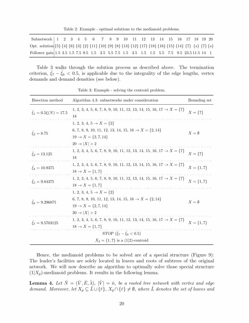
Table 2: Example - optimal solutions to the medianoid problems.

Subnetwork 1 2 3 4 5 6 7 8 9 10 11 12 13 14 15 16 17 18 19 20

Opt. solution {5} {4} {6} {3} {2} {11} {10} {9} {8} {13} {12} {17} {18} {16} {15} {14} {7} {s} {7} {s}Follower gain 1.5 3.5 1.5 7.5 9.5 1.5 3.5 5.5 7.5 1.5 3.5 1.5 1.5 5.5 7.5 9.5 23.5 11.5 14 1

Table 3 walks through the solution process as described above. The terminationcriterion, ξ7 − ξ6 < 0.5, is applicable due to the integrality of the edge lengths, vertexdemands and demand densities (see below).

Table 3: Example - solving the centroid problem.

Bisection method Algorithm 4.3: subnetworks under consideration Bounding set

ξ1 = 0.5ξ(N) = 17.51, 2, 3, 4, 5, 6, 7, 8, 9, 10, 11, 12, 13, 14, 15, 16, 17 → X = {7}

X = {7}18

ξ2 = 8.75

1, 2, 3, 4, 5 → X = {2}

X = ∅6, 7, 8, 9, 10, 11, 12, 13, 14, 15, 16 → X = {2, 14}19 → X = {2, 7, 14}20 → |X| > 2

ξ3 = 13.1251, 2, 3, 4, 5, 6, 7, 8, 9, 10, 11, 12, 13, 14, 15, 16, 17 → X = {7}

X = {7}18

ξ4 = 10.93751, 2, 3, 4, 5, 6, 7, 8, 9, 10, 11, 12, 13, 14, 15, 16, 17 → X = {7}

X = {1, 7}18 → X = {1, 7}

ξ5 = 9.843751, 2, 3, 4, 5, 6, 7, 8, 9, 10, 11, 12, 13, 14, 15, 16, 17 → X = {7}

X = {1, 7}18 → X = {1, 7}

ξ6 = 9.296875

1, 2, 3, 4, 5 → X = {2}

X = ∅6, 7, 8, 9, 10, 11, 12, 13, 14, 15, 16 → X = {2, 14}19 → X = {2, 7, 14}20 → |X| > 2

ξ7 = 9.57031251, 2, 3, 4, 5, 6, 7, 8, 9, 10, 11, 12, 13, 14, 15, 16, 17 → X = {7}

X = {1, 7}18 → X = {1, 7}

STOP (ξ7 − ξ6 < 0.5)

X2 = {1, 7} is a (1|2)-centroid

Hence, the medianoid problems to be solved are of a special structure (Figure 9):The leader’s facilities are solely located in leaves and roots of subtrees of the originalnetwork. We will now describe an algorithm to optimally solve those special structure(1|Xp)-medianoid problems. It results in the following lemma.

Lemma 4. Let N = (V , E, λ), |V | = n, be a rooted tree network with vertex and edgedemand. Moreover, let Xp ⊆ L∪{r}, Xp∩{r} 6= ∅, where L denotes the set of leaves and

20

r corresponds to the root of the tree network with degree 1. Then the problem of finding adiscrete, binary (1|Xp)-medianoid can be solved with time complexity O(np).

The algorithm is composed of six stages.

1. Collapse, O(n)

2. Label, O(n)

3. Rearrange, O(p2)

4. Construct chain functions, O(np)

5. Calculate distances of facilities in Xp, O(p2)

6. Evaluate, O(np)

In the following we will describe each of the six stages in detail. We denote the elementsof the set Xp by xi, i = 1, ..., p, where, without loss of generality, x1 corresponds to theleader’s facility located in the root r.

Collapse: Consider a leaf x /∈ Xp and let x′ 6= r be the father of x. It is easy to see thatWF (x|Xp) ≤ WF (x′|Xp). Therefore, we may construct an auxiliary tree network N ′ bymerging x and x′ to define a vertex vx,x′ with π(vx,x′) = π(x) + π(x′) + λ([x′, x])δ([x′, x])to replace x′. Any (1|Xp)-medianoid on N ′ corresponds to a (1|Xp)-medianoid on N .The transformation is straight forward: Let vx,x′ be an optimal solution to the (1|Xp)-medianoid problem on N ′; then x′ is the corresponding (1|Xp)-medianoid on N . Thisidea of merging vertices can be repeated until every leaf of the resulting auxiliary treenetwork is either a child of r or an element of Xp. This can be achieved by performing adepth first search traversal of the tree network of time complexity O(n). An example withXp = {x1, x2, x3, x4, x5} is given in Figure 10. Since vertex 13 is a leaf without being aleader’s location, we may merge vertices 13 and 12. The resulting vertex can subsequentlybe merged with vertices 11 and 6.

Observe that for p ≤ 2 we are left with a chain network (see Section 4.1). Therefore,in what follows, we will restrict our attention to the nontrivial case p > 2. Moreover, toease notation, we will omit the superscript ′ when referring to the collapsed tree networkand its vertex set, i.e. we will keep using the notation that has been introduced in Lemma4.

Label: It is well known that the vertices of a tree network can be labeled in lineartime such that hereafter the nearest common ancestor of any pair of vertices as well astheir distance can be computed in constant time. See, for example, Alstrup et al. [32] andthe references therein.

Rearrange: This stage aims at finding a permutation [xµ1 , ..., xµp−1] of the elements

xi, i = 2, ...p. Roughly speaking, this permutation is such that the customers located onthe unique path that connects a superordinated vertex of the permutation to the rootare guaranteed not to accommodate their demand at a leader’s facility located at a sub-ordinated element of the permutation (or to be indifferent about accommodating theirdemand at one of the two corresponding leader’s facilities). Additionally, in combinationwith the subsequent stages of the algorithm, the permutation eventually guarantees thateach customer accommodates his demand at a single facility by grouping the leader’s facil-ities according to their nearest common ancestors. The permutation is being determinedby applying a three stage algorithm:

21

1

2

3

4

5

6

7 8

10

9

x2

x3 x4

x1ˆ ˆ( ( r1), ( r1))

(1,1)

(1,1)

(1,1) (2,1)

(2,1)

(2,2 ) (3,1)

(1,1) (1,1) (1,1)

2

2

2

6

1

1

1

1

ˆ( r ) 1

1

7

x5

11

13

12

(1,1)

(2,1)

2

1

1

(1,1)

r

(a) Original tree network N .

1

2

3

4

5

6'

7 8

10

9

x2

x3 x4

x1

(1,1)

(1,1) (2,1)

(2,1)

(2,2 ) (3,1)

(1,1) (1,1) (1,1)

2

2

2

6

1

1

9

1

ˆ( r ) 1

1

7

x5

ˆ ˆ( ( r1), ( r1))

(1,1)

r

(b) Auxiliary tree network N ′.

Figure 10: Collapsing stage.

1. Calculate d(r, xi) for all i = 2, ...p by use of the vertex labels (Stage 2) (timecomplexity O(p)).

2. Sort the elements xi, i = 2, ...p, in the order of increasing distances d(r, xi). Wemay, for example, apply mergesort (time complexity O(p log p), cf. Cormen et al.[33]). The sorting algorithm results in an array L of length p− 1 with the smallestelement in the first position, denoted by L[1].

3. Call Algorithm 4.4 to determine the desired permutation P . We denote the i-thposition of the permutation P by P [i]. Using a linked list data structure, thealgorithm has time complexity O(p2).

Algorithm 4.4 Generate rearranged facilities.

1: initialize P2: pos := 0, lastpos := 2, depth := 03: P [1] = L[1], P [2] = L[2]4: for i = 3 to p− 1 do5: pos = 06: depth = d(r, nca(L[i], P [1]))7: for j = 2 to lastpos do8: if d(r, nca(L[i], P [j])) > depth then9: depth = d(r, nca(L[i], P [j]))

10: pos = j + 111: end if12: end for13: if pos = 0 then14: if d(r, nca(L[i], P [1])) > d(r, nca(L[i], P [2])) then15: pos = 216: else

22

17: pos = lastpos+ 118: end if19: end if20: P [pos] = L[i]21: lastpos = lastpos+ 122: end for

Let us denote the unique path that connects xµj to the root r by cµj for each j =1, ..., p − 1. Then the three stage rearranging process is such that for any pair k, l ∈{1, ..., p − 1} with k < l there exists a µm, m ≤ k such that d(xµm , z) ≤ d(xµl , z) for allpoints z on cµk , even if d(xµl , r) < d(xµk , r).

We conclude by revisiting the example of Figure 10b in Table 4.

Table 4: Rearranging stage for the example in Figure 10b.

Steps 1 and 2: distances: sorted distances:

i 2 3 4 5

d(r, xi) 5 4 3 5

i 4 3 2 5

d(r, xi) 3 4 5 5

Alg. 4.4, initialization: L = [x4, x3, x2, x5] P = [x4, x3]

Alg. 4.4, i = 3: insert x2:

nca(x4, x2) = 1, d(r, 1) = 1

nca(x3, x2) = 2, d(r, 2) = 3 P = [x4, x3, x2]

Alg. 4.4, i = 4: insert x5:

nca(x4, x5) = 6′, d(r, 6′) = 2

nca(x3, x5) = 1, d(r, 1) = 1

nca(x2, x5) = 1, d(r, 1) = 1 P = [x4, x5, x3, x2]

When inserting x2, the algorithm compares the “depth” of the nearest common an-cestors of x2 and the facilities x4 and x3 in the tree network. Since the latter nearestcommon ancestor is located deeper in the network, x2 is inserted after x3. Similarly, x5needs to be paired with facility x4. Thus, the procedure terminates with xµ2 = x5 andxµ3 = x3 although d(r, x3) = 4 < d(r, x5) = 5 because x4 will always be closer to anypoint on chain [r, 1, 6′, 8, 9, 10] than x3.

Construct chain functions: As in the case of chain networks (Section 4.1), we cannow define “chain functions” fµi(yµi) for all i = 1, ..., p− 1, where yµi are local variablesthat correspond to the distance of a point on chain cµi to the root r of the collapsed treenetwork. In the following we will denote the vertices of a chain cµi in the sequence of

increasing distance to the root r by v1µi , ..., vlµi+1µi , where lµi is the number of edges on the

unique path from r to xµi . In contrast to Section 4.1 we will now have to assign eachvertex/edge customer to a unique chain. We do so by considering the permutation P thatresults from the rearranging stage. For any i > 1, we denote the vertex nca(xµi−1

, xµi) by

23

vsµi , where 1 ≤ s ≤ lµi , and we define

fµi(yµi) :=

0 if yµi ≤ d(r, vsµi),

δ([vsµi , vs+1µi ])(yµi − d(r, vsµi)) if d(r, vsµi) < yµi ≤ d(r, vs+1

µi ),...

...u−1∑j=s

[δ([vjµi , vj+1µi ])λ([vjµi , v

j+1µi ]) + π(vjµi)]

− π(vsµi) + π(vuµi)

+ δ([vuµi , vu+1µi ])(yµi − d(r, vuµi))

if d(r, vuµi) < yµi ≤ d(r, vu+1µi ),

......

lµi−1∑j=s

[δ([vjµi , vj+1µi ])λ([vjµi , v

j+1µi ]) + π(vjµi)]

− π(vsµi) + π(vlµiµi )

+ δ([vlµiµi , v

lµi+1µi ])(yµi − d(r, v

lµiµi ))

if d(r, vlµiµi ) < yµi ≤ d(r, v

lµi+1µi ),

lµi∑j=s

[δ([vjµi , vj+1µi ])λ([vjµi , v

j+1µi ]) + π(vjµi)]

− π(vsµi) + π(vlµi+1µi )

if d(r, vlµi+1µi ) < yµi .

(34)

For i = 1 we define vsµ1 := r and fµ1(yµ1) in analogy to equation (30).A simple O(np) procedure to construct the chain functions determines the chains cµi

for all i = 1, ..., p − 1 by performing a depth first search traversal of the collapsed treenetwork and, afterwards, generates the needed coefficients by considering all edges of thecollapsed tree network at most p times. After having constructed a chain function cµi , wecan evaluate it in constant time for a given yµi .

For our example, the chain functions fµ1(yµ1), ..., fµ4(yµ4) for P = [x4, x5, x3, x2] aredepicted in Figure 11. Since, for instance, nca(x4, x5) = 6′, we have fx5(yx5) = 0 forall yx5 ≤ d(r, 6′). Hence, the vertex demand of the vertices r and 1 as well as the edgedemand of the edges [r, 1] and [1, 6′] is uniquely assigned to chain cx4 .

Calculate distances of facilities in Xp: Determine

D(xµi) := min{d(r, xµi),min{d(xµi , xµj)|j < i}} (35)

for all i = 2, ..., p−1 and denote one of the corresponding vertices by V (D(xµi)). This canobviously be achieved in O(p2) time. Moreover, we equivalently define D(xµ1) := d(r, xµ1)and V (D(xµ1)) := r. The example is revisited in Table 5.

Evaluate: Consider a vertex v ∈ V \{Xp} of the collapsed tree network as a potentialfollower’s location and let k = min{i|v is a vertex on chain cµi , i ∈ {1, ..., p − 1}}. Thenwe can easily determine an open interval ]acµj , bcµj [ with acµj ≤ bcµj of customers whoaccommodate their demand at v for each chain cµj , j = 1, ..., p− 1 in analogy to Section4.1.

24

1 2 3

4 4f ( y )

4

1 6' 7

1 1f ( y )

1 6' 10

2 2f ( y )

8 9

1 2 5

3 3f ( y )

5

10

15

5

10

5

10

15

5

10

1y

2y

3y

4y

r

r r

r

Figure 11: Functions fµi(yµi

), i = 1, ..., 4, for the example in Figure 10b.

Table 5: D(xµi) and V (D(xµi

)), i = 1, ..., 4, for the example in Figure 10b.

i 1 2 3 4

xµi x4 x5 x3 x2

D(xµi) 3 4 4 3

V (D(xµi)) r 7 r 5

25

• For all cµj with j > k:

acµj = 0, (36)

bcµj =

{d(r, xµj)−

d(v,xµj )

2if d(v, xµj) < D(xµj),

0 else.(37)

• For all cµj with j < k, j 6= 1:

acµj =

{d(r, v)− d(V (D(xµj )),v)

2if d(r, v) < d(r, xµj) and d(xµj , v) < D(xµj),

0 else,(38)

bcµj =

{d(r, xµj)−

d(v,xµj )

2if d(r, v) < d(r, xµj) and d(xµj , v) < D(xµj),

0 else.(39)

• For cµk :

acµk = d(r, v)− d(V (D(xµk)), v)

2, (40)

bcµk =d(r, xµk) + d(r, v)

2. (41)

• For cµ1 , if k 6= 1:

acµ1 =

{d(r,v)

2if d(r, v) < d(r, xµ1) > d(v, xµ1),

0 else,(42)

bcµ1 =

{d(r, xµ1)−

d(v,xµ1 )

2if d(r, v) < d(r, xµ1) > d(v, xµ1),

0 else.(43)

Observe that there might exist points of the collapsed tree network that are containedin multiple intervals ]acµj , bcµj [, j ∈ {1, ..., p− 1}. However, by definition of equation (34)

and fµ1(yµ1), only one of the corresponding chain functions fµj(yµj) may have a valuelarger than zero at each of these points, so that the related demand will only be consideredonce in the subsequent calculation of the actual follower’s market share WF (v|Xp). Inanalogy to Section 4.1 we get

WF (v|Xp) =

p−1∑j=1

WcµjF (v|Xp), (44)

where

WcµjF (v|Xp) =

{fµj(bcµj )− fµj(acµj ) if d(r, vsµj) ≥ acµj ,

fµj(bcµj )− fµj(acµj )− π(acµj ) else,(45)

corresponds to the portion of the total follower’s market share that is induced by chaincµj for any j ∈ {1, ..., p− 1}.

26

Equations (36)-(45) can be evaluated in constant time for a given v, so that we are nowable to determine a (special structure) discrete, binary (1|Xp)-medianoid with time com-plexity O(np) as claimed in Lemma 4. The following algorithm stores (1|Xp)-medianoidsin the set Y ; the corresponding follower’s market share equals W ∗.

Algorithm 4.5 Evaluate.

1: Y := ∅, W := 0, W ∗ := 02: for all v ∈ V \ {Xp} do3: W = 04: for j = 1 to p− 1 do5: W = W +W

cµjF (v|Xp) (Equations (36)-(45))

6: end for7: if W > W ∗ then8: Y = {v}9: W ∗ = W

10: else if W = W ∗ then11: Y = Y ∪ {v}12: end if13: end for14: if Y = ∅ then15: Y = {r}16: end if

Let us consider our example with the follower’s location in vertex v = 6′, i.e. k = 1.We get acµ1 = 2 − 2/2 = 1, bcµ1 = (3 + 2)/2 = 2.5, acµ2 = 0, bcµ2 = 5 − 3/2 = 3.5,acµ3 = 0, bcµ3 = 0, acµ4 = 0, bcµ4 = 0 and WF (6′|Xp) = 15.5. Analogously, one computesthe follower’s market share when locating in vertex 1, 2, 3, 8 or 9. By comparison of thesevalues we find vertex 6′ to be the (1|X5)-medianoid.

We may now conclude this section with the main result in Theorem 6.

Theorem 6. The problem of finding a discrete, binary (1|p)-centroid of a tree net-work N = (V,E, λ) with vertex and edge demand can be solved with time complexityO(n2p log ξ(N)).

Proof. We apply bisection on the interval [0, ξ(N)] to find the smallest value ξ such thata ξ-bounding set with at most p elements exists. The termination criterion described inthe proof of Theorem 5 can be adapted to the case at hand.

5. Conclusion

In this paper we have analyzed a classical sequential location problem on networks,the (r|p)-centroid problem under a binary choice rule. Differing from the majority ofprevious publications, we have considered networks with both, vertex and edge demand.The corresponding follower problem is known to be NP-hard even on networks with edgedemand only [14]. We have proven that this remains true for the (r|p)-centroid prob-lem. On tree networks, however, an efficient algorithm to determine a (1|p)-centroid has

27

been derived, after having restricted the location sites to the vertex set of the underlyingnetwork (discrete problem class). Bilevel programming models have been presented forthe discrete (r|p)-centroid problem on general networks with vertex and edge demand.Computational results based on these models indicate, that heuristics will need to ap-proximate the follower’s response to a given set of leader’s locations. An upper bound onthe follower’s optimal market share has previously been introduced for the case of vertexdemand only. We have shown that this bound can be adapted to the case of vertex andedge demand. Future research topics (cf. also Section 3.4) include the application of non-uniform demand densities or different types of choice rules, as, for example, proportionalor partially binary choice rules.

Appendix A. Computational results

Note: “-” marks trivial instances with r + p ≥ n.

Table A.6: Computational results - Model BBNP with fixed set of leader’s locations, p = 1.

avg. comp. time instances not solved to optimality

r # of vertices [sec.] # average gap [%]

1

5 0.0188 0 010 0.1062 0 015 0.3963 0 020 1.0048 0 025 2.6973 0 0

2

5 0.0967 0 010 0.4306 0 015 1.5272 0 020 3.9342 0 025 11.8092 0 0

3

5 0.0361 0 010 0.2915 0 015 6.0265 0 020 28.1928 0 025 202.638 0 0

4

5 - - -10 0.4084 0 015 35.2106 0 020 297.308 0 025 1424.61 4 29.05

Table A.7: Computational results - Model BBNP with fixed set of leader’s locations, p = 2.

avg. comp. time instances not solved to optimality

r # of vertices [sec.] # average gap [%]

1

5 0.0157 0 010 0.0875 0 015 0.2605 0 020 0.6396 0 025 2.0358 0 0

2

5 0.0188 0 010 0.0828 0 015 0.3199 0 020 1.0142 0 025 4.7645 0 0

3

5 - - -10 0.1014 0 0

28

15 0.5302 0 020 2.672 0 025 19.9147 0 0

4

5 - - -10 0.1329 0 015 1.2654 0 020 10.329 0 025 114.313 0 0

References

[1] Hotelling H. Stability in competition. The Economic Journal 1929;39(153):41–57.

[2] Drezner T. Competitive facility location in the plane. In: Drezner Z, editor. FacilityLocation - A Survey of Applications and Methods. New York: Springer; 1995, p.285–300.

[3] Eiselt HA, Laporte G, Thisse JF. Competitive location models: A framework andbibliography. Transportation Science 1993;27(1):44–54.

[4] Eiselt HA, Laporte G. Sequential location problems. European Journal of Opera-tional Research 1996;96(2):217–31.

[5] Kress D, Pesch E. Sequential competitive location on networks. European Journalof Operational Research 2012;217(3):483–99.

[6] Plastria F. Static competitive facility location: An overview of optimisation ap-proaches. European Journal of Operational Research 2001;129(3):461–70.

[7] Serra D, ReVelle C. Competitive location in discrete space. In: Drezner Z, editor.Facility Location - A Survey of Applications and Methods. New York: Springer; 1995,p. 367–86.

[8] ReVelle CS, Eiselt HA. Location analysis: A synthesis and survey. European Journalof Operational Research 2005;165(1):1–19.

[9] Hooker JN, Garfinkel RS, Chen CK. Finite dominating sets for network locationproblems. Operations Research 1991;39(1):100–18.

[10] Hay DA. Sequential entry and entry-deterring strategies in spatial competition.Oxford Economic Papers 1976;28(2):240–57.

[11] Prescott EC, Visscher M. Sequential location among firms with foresight. The BellJournal of Economics 1977;8(2):378–93.

[12] von Stackelberg H. Marktform und Gleichgewicht. Vienna: Springer; 1934.

[13] Hakimi SL. On locating new facilities in a competitive environment. EuropeanJournal of Operational Research 1983;12(1):29–35.

[14] Dasci A, Eiselt H, Laporte G. On the (r,Xp)-medianoid problem on a network withvertex and edge demands. Annals of Operations Research 2002;111(1):271–8.

29

[15] Okunuki KI, Okabe A. Solving the Huff-based competitive location model on anetwork with link-based demand. Annals of Operations Research 2002;111(1-4):239–52.

[16] Spoerhase J, Wirth HC. (r, p)-centroid problems on paths and trees. TheoreticalComputer Science 2009;410(47-49):5128–37.

[17] Bandelt HJ. Networks with Condorcet solutions. European Journal of OperationalResearch 1985;20(3):314–26.

[18] Bauer A, Domschke W, Pesch E. Competitive location on a network. EuropeanJournal of Operational Research 1993;66(3):372–91.

[19] Swamy MNS, Thulasiraman K. Graphs, Networks, and Algorithms. New York:Wiley; 1981.

[20] Hakimi SL. Locations with spatial interactions: Competitive locations and games. In:Mirchandani PB, Francis RL, editors. Discrete Location Theory. New York: Wiley;1990, p. 439–78.

[21] Hansen P, Labbe M. Algorithms for voting and competitive location on a network.Transportation Science 1988;22(4):278–88.

[22] Hansen P, Thisse JF. Outcomes of voting and planning: Condorcet, Weber andRawls locations. Journal of Public Economics 1981;16(1):1–15.

[23] Dobson G, Karmarkar US. Competitive location on a network. Operations Research1987;35(4):565–74.

[24] Dempe S. Foundations of Bilevel Programming. Kluwer Academic Publishers; 2002.

[25] Bard JF. Practical Bilevel Optimization - Algorithms and Applications. Dordrecht:Kluwer; 1998.

[26] Benati S, Laporte G. Tabu search algorithms for the (r|Xp)-medianoid and (r|p)-centroid problems. Location Science 1994;2(4):193–204.

[27] Nemhauser GL, Wolsey LA. Integer and Combinatorial Ooptimization. New York:Wiley; 1999.

[28] Jaramillo JH, Bhadury J, Batta R. On the use of genetic algorithms to solve locationproblems. Computers & Operations Research 2002;29(6):761–79.

[29] Arostegui Jr. MA, Kadipasaoglu SN, Khumawala BM. An empirical comparisonof tabu search, simulated annealing, and genetic algorithms for facilities locationproblems. International Journal of Production Economics 2006;103(2):742–54.

[30] Garey MR, Johnson DS. Computers and Intractability - A Guide to the Theory ofNP-Completeness. New York: Freeman; 1979.

30

[31] Megiddo N, Zemel E, Hakimi SL. The maximum coverage location problem. SIAMJournal on Algebraic and Discrete Methods 1983;4(2):253–61.

[32] Alstrup S, Gavoille C, Kaplan H, Rauhe T. Nearest common ancestors: A surveyand a new algorithm for a distributed environment. Theory of Computing Systems2004;37(3):441–56.

[33] Cormen TH, Leiserson CE, Rivest RL, Stein C. Introduction to Algorithms. Cam-bridge: The MIT press; 2nd ed.; 2001.

31