Embed Size (px)
Citation preview
HAL Id: tel-00608229https://tel.archives-ouvertes.fr/tel-00608229
Submitted on 12 Jul 2011
HAL is a multi-disciplinary open accessarchive for the deposit and dissemination of sci-entific research documents, whether they are pub-lished or not. The documents may come fromteaching and research institutions in France orabroad, or from public or private research centers.
L’archive ouverte pluridisciplinaire HAL, estdestinée au dépôt et à la diffusion de documentsscientifiques de niveau recherche, publiés ou non,émanant des établissements d’enseignement et derecherche français ou étrangers, des laboratoirespublics ou privés.
Research of Nonlinear System High Order Sliding ModeControl and its Applications for PMSM
Yi-Geng Huangfu
To cite this version:Yi-Geng Huangfu. Research of Nonlinear System High Order Sliding Mode Control and its Applica-tions for PMSM. Chemical and Process Engineering. Northwestern Polytechnical University (Chine),2010. English. <NNT : 2010BELF0130>. <tel-00608229>

A Dissertation for the Degree of Philosophy Doctor
Research of Nonlinear System High Order Sliding Mode Control and its Applications
for PMSM
by
Huangfu Yi-geng
Supervised by
Prof. Abdellatif MIRAOUI
and
Prof. LIU Wei-guo
University of Technology of Belfort-Montbéliard
And
Northwestern Polytechnical University
January, 2010
II
ACKNOWLEDGMENTS
My great gratitude goes primarily to my adviser, Professor Abdellatif MIRAOUI and
Professor Weiguo LIU, for intellectual support, encouragement, and enthusiasm which made this
dissertation possible.
I also wish to thank my committee members, Professor Taha BOUKHOBZA and Professor
Ruiqing MA, for their valuable advices on this dissertation.
Further, I am grateful to my parents for their prayers, guidance and support throughout my
education. Their inspiration and encouragement has been invaluable. Finally, thanks to my wife,
Di WU, for her love, support and patience especially during the write-up and viva preparation
when she has to handle all the housework alone.
I thank Chinese Scholarship Council (CSC) for their financial support when I studied in
France.
�
III
ABSTRACT
Nonlinear system control has been widely concern of the research. At present, the nonlinear
system decoupling control and static feedback linearization that based on the theory of differential
geometry brought the research getting rid of limitation for local linearization and small scale
motion. However, differential geometry control must depend on precise mathematical model. As a
matter of fact, the control system usually is with parameters uncertainties and output disturbance.
In this thesis, nonlinear system of control theory has been studied deeply. Considering sliding
mode variable structure control with good robust, which was not sensitive for parameters
perturbation and external disturbance, the combination idea of nonlinear system and sliding mode
controls was obtained by reference to the large number of documents. Thus, it not only can
improve system robustness but solve the difficulties problem of nonlinear sliding mode surface
structure. As known to all, traditional sliding mode had a defect that is famous chattering
phenomenon. A plenty of research papers focus on elimination/avoidance chattering by using
different methods. By comparing, the document is concerned with novel design method for high
order sliding mode control, which can eliminate chattering fundamentally. Especially, the
approach and realization of nonlinear system high order sliding mode control is presented in this
paper.
High order sliding mode technique is the latest study. This thesis from the theory analysis to
the simulation and experiment deeply study high order sliding mode control principle and its
applications. By comparison, the second order sliding mode control law (also known as dynamic
sliding mode control, DSM) may be effective to eliminate the chattering phenomenon. But it is
still unable to shake off the requirement of system relative degree. Therefore, arbitrary order
sliding mode controller is employed, whose relative degree can equal any values instead of one.
The robot car model adopted high order sliding mode is taken as an example. The simulation
results show that the tracking control is effective.
In the control systems design, it is very often to differentiate the variables. Through the
derivation of sliding mode, the expression of sliding mode differential value is obtained. The
simulation results certificate sliding mode differentiator with robustness and precision. At the
same time, the differentiator for arbitrary sliding mode is given to avoiding conventional complex
numerical calculation. It not only remains the precision of variables differential value, but also

IV
obtains the robustness. A direct application is simplification for high order sliding mode
controller.
Due to its inherent advantages, the permanent magnet synchronous motor (PMSM) deserves
attention and is the most used drive in machine tool servos and modern speed control applications.
For improving performance, this paper will applied nonlinear high order sliding mode research
achievement to MIMO permanent magnet synchronous motor. It changes the coupling nonlinear
PMSM to single input single output (SISO) linear subsystem control problem instead of near
equilibrium point linearization. Thereby, the problem of nonlinear and coupling for PMSM has
been solved. In addition, Uncertainty nonlinear robust control system has been well-received study
of attention. Because the robust control theory is essentially at the expense of certain performance.
This kind of robust control strategy often limits bandwidth of closed loop, so that system tracking
performance and robustness will be decreased. So, sliding mode control is an effective approach
for improving system robust. This thesis first proposed a robust high order sliding mode controller
for PMSM. The system has good position servo tracking precision in spite of parameters
uncertainties and external torque disturbance.
On this basis, According to the principle of high order sliding mode, as well as differentiator,
the state variables of PMSM are identified online firstly and successfully. The results of
simulation indicate observe value has high precision when sliding mode variable and its
differentials are convergent into zero. The same theory is used in external unknown torque
disturbance estimation online for PMSM. As if, load torque will no longer be unknown
disturbance. System performance can be improved greatly. It establishes theoretical foundation for
the future applications.
At the end of paper, using advanced half-physical platform controller dSPACE to drive a
PMSM, hardware experiment implement is structured completely. The experiment results
illustrate that PMSM adopting precious feedback linearization decoupling and high order sliding
mode controller can realize system servo tracking control with good dynamic and steady
character.
Keywords: Nonlinear system, Differential geometry theory, Precious feedback linearization,
High order sliding mode, Differentiator, Permanent magnet synchronous motor, dSPACE
5
CATALOGUE
ACKNOWLEDGMENTS ............................................................................................................. II
ABSTRACT ................................................................................................................................... III
CATALOGUE ................................................................................................................................. 5
Chapter 1 Introduction ................................................................................................................ 7
1.1 Introduction ....................................................................................................................... 7
1.2 The developing history and present state of nonlinear control theories .......................... 11
1.2.1 The developing history of nonlinear control theories ..................................................... 11
1.2.2 The present state of nonlinear control theories ............................................................... 12
1.3 The basic principle of sliding mode control theory ......................................................... 13
1.3.1 Basic concepts ................................................................................................................. 14
1.3.2 The principle, merits and drawbacks of sliding mode control ........................................ 18
1.3.3 Chattering problem and solving ...................................................................................... 21
1.4 The application and research of nonlinear sliding mode control systems ....................... 27
1.5 The main research contents of the paper ......................................................................... 28
Chapter 2 Nonlinear system high order sliding mode control ............................................... 31
2.1 Second order sliding mode control.................................................................................. 32
2.2 Simulation example (levant,2003) .................................................................................. 36
2.3 Arbitrary order sliding mode control .............................................................................. 41
2.4 Simulation example ......................................................................................................... 43
2.5 Quasi-continuous high order sliding mode control ......................................................... 47
2.6 Summary ......................................................................................................................... 51
Chapter 3 Robust exact high order sliding mode differentiator ............................................ 52
3.1 Robust sliding mode differentiator .................................................................................. 52
3.2 Numerical simulation ...................................................................................................... 54
3.3 Arbitrary order sliding mode differentiator ..................................................................... 56
3.4 Simulation example ......................................................................................................... 58
3.5 Summary ......................................................................................................................... 60
Chapter 4 Application — Nonlinear permanent magnetic synchronous motor high order
sliding mode control ...................................................................................................................... 62
4.1 Mathematical model of PMSM ....................................................................................... 63
4.2 Robust high order sliding mode control for PMSM ........................................................ 65
6
4.3 State variable estimation for PMSM ............................................................................... 74
4.4 Disturbance torque estimation for PMSM ...................................................................... 81
4.5 Summary of this chapter ................................................................................................. 83
Chapter 5 Experimental system based on dSPACE ................................................................ 84
5.1 Introduction of dSPACE control platform ....................................................................... 84
5.2 PMSM control system based dSPACE ............................................................................ 85
5.3 Development steps of control system.............................................................................. 87
5.4 Experiment results and analysis ...................................................................................... 89
5.5 Summary of this chapter ................................................................................................. 95
Chapter 6 Summary ................................................................................................................... 96
6.1 The chief work and research results of the paper ............................................................ 96
6.2 Several issues to be resolved ........................................................................................... 98
Reference...................................................................................................................................... 100
Publications ................................................................................................................................. 112

7
Chapter 1 Introduction
In recent years, the robustness control of nonlinear system has already become
one of the main research areas for numerous researchers. At present, the ideas applied
to solve the problem mainly include nonlinear ∞H ,adapting control,stepping control,
sliding mode control and so on. The document makes an intensive study into
nonlinear system control theories, and meanwhile combines with a technology named
high order sliding mode, which ensures the accuracy of decoupling control and
improves the robustness of systems.
The contents of chapter 1 are shown as follows. Section 1 simply summarizes the
application of nonlinear system and its technology background. Section 2 introduces
the development and current situation of nonlinear system control theories. Section 3
presents the fundamental principles of sliding mode control technology. Section 4
analyzes the application of sliding mode control in nonlinear system. Section 5 shows
chief research contents, structural arrangement and creative points of the paper.
1.1 Introduction
The historical process in which human beings know and change the world is
always a gradual developing process from low class to top grade, from simplicity to
complexity, from surface to inner. And the same to the aspect of control area, the early
research on control system is all linear. For example, Watt steam-engine regulator,
adjusting the liquid level and so on. It was limited by the current knowledge of human
being on the natural phenomena and the ability to deal with the practical problems, for
the linear system’s physical description and its mathematical solving is much easier to
achieve. In addition, it has already formed a perfect series of linear theories and
research methods. By contrast, for nonlinear systems, except for minority situations,
so far there hasn’t been a feasible series of general methods. Even if there are several
methods that will only solve problems belonging to one category, they can’t be
applied generally. Accordingly, that is to say, how we study and dispose the nonlinear
system control is still staying at the elementary stage on the whole. Besides, from the
viewpoint of the accuracy we need to control the system, it will get a satisfactory
result within limits to utilize the linear system theories to deal with the most
technology problems in engineering at present. Therefore, the nonlinear factors of one
8
real system are often neglected on purpose or substituted for various linear relations.
To sum up, that is the principal cause which prompts the linear system theories to
develop quickly and become correspondingly perfect day by day and restricts the
nonlinear system theories from getting much attention and developing over a long
term.
The present system has become more and more complicated, integrative and
intelligent, while the request on its performance has become more and more strict.
The research on the motion laws and analytical methods of the nonlinear system has
already become a significant branch in the automatic control theories. Strictly
speaking, the real systems mostly belong to nonlinear system. By contrast, linear
systems are ideal models in order to simplify the mathematic problems. The contrast
between linearity and non linearity is that the last one is a "non propriety". Yet, this
main characteristic is a negation of propriety and cannot be used to have any
unification in the methods or techniques used to analyze and control such systems. As
a result, it determines the complexity on research. For nonlinear systems, in the past
the researchers adopted the method of approximate linearization to linearize them,
such as Taylor unfolding method, Jacobian matrix method and so on. These methods
should be applied to nonlinear systems under the better initial value and the higher
accuracy, which are effective to dispose the systems with the working point moving
on a small scale. At the same time, the working point in practical systems is always
moving. If the point moves beyond the scale or some component works in the
nonlinear area, the output will bring strange phenomenon which can not be explained
by linear theories. In addition, there are still some running behaviors such as
asynchronous suppression, bifurcation, chaos, strange attractors from complicated
systems which belong to nonlinear phenomenon in substance. Obviously, they can’t
be analyzed by means of linear models. Therefore, the nonlinear problems in
mathematics should be solved with the theories and methods in the nonlinear science.
During the last two decades of the 20th century, differential geometry theory and
its applications have developed fast, so that the research on nonlinear system control
theories and their applications got a breakthrough improvement. With the help of
differential geometry theory, necessary and sufficient conditions (Hermann,1977;
Isidori,96) of controllability and observability and were set up systematically via the
research on the dependency relationships among the state, input and output of
nonlinear system, which were studied by the basic tools such as Lie bracket. The

9
research models of differential geometry control theory get rid of partial linearization
and movement on a small scale and realize the global analysis and synthesization on
the dynamic systems. Nonlinear system control theory based on differential geometry
theory realizes the linearization of nonlinear systems by means of state feedback and
coordinate transformation under some conditions on the control. The point that
doesn’t neglect any high order nonlinear item in the linearization progress is different
from traditional approximate linearization methods. So the linearization is not only
accurate but also global, that is to say, it can be applied to the whole scale with
definitions (Howze,1973). Among others, the linearization based on differential
geometry theory in the algorithm still need the accurate nonlinear system models.
However, it’s impractical to use an accurate mathematic model to describe the
dynamic character for a system. So it’s inevitable to exist the factors such as
parameter uncertainty, time-varying parameters, time delay, external disturbance
which will have an influence on controller design. Accordingly, it’s also considerably
crucial to research on the robustness of nonlinear systems.
In the recent years, nonlinear ∞H robust control, the fuzzy control, expert
system, neural nets, adapting control, stepping control, sliding mode control and etc.
have become the main research aspects. In addition, there are still several research
results from some literatures which combine the control technologies together to
improve them. Meanwhile, they are all accomplished under the more restrictive
conditions on mathematic models. Among the researches on various nonlinear control
techniques, each one has its own property. For it’s not sensitive for the changing
structure of sliding mode to react on the perturbation of system parameters and
external elements, while for it’s of strong robustness and its control structure design is
simple to come true, sliding mode control has been an indispensable branch in the
system robustness control theories. How to utilize the nonlinear coordinate change of
diffeomorphism to devise sliding controllers is a point for the sliding mode control of
nonlinear systems. In the process, it’s supposed to ensure sliding mode to be strong
robustness, to realize the linearization easily and to be immune to uncertain system
parameters.
As we known, permanent magnet synchronous motor has so many advantages
such as compact structure, high power density, high air-gap flux, no conversion spark
and high torque inertia ratio, which is widely used in servo systems (Caravani,1998;
Glumineau,1993; Ziribi,2001). Considering permanent magnet synchronous motor is

10
a nonlinear system with MIMO and coupling, which includes the product term of
angular velocity and d-q axis current, it must achieve decoupling and linearization of
the system to get the accurate control performance. Adopting permanent magnet
synchronous motor as a typical application example in nonlinear kinetic control servo
systems has universal significance. Permanent magnet synchronous motor is a MIMO
and nonlinear time-varying system. In the past, adopting the traditional linearization
can only realize partial approximation to get a mathematic model which can not
describe the dynamic and static process of system accurately. The practice
demonstrates that control method based on approximate linearization is so limited that
it can not adjust to the converting system parameters and satisfy the request of wide
speed regulation. And feedback linearization based on differential geometry
overcomes the shortcoming of traditional linearization that the balance point can only
keep steady on a small scale. So it’s desire to need a control algorithm with good
robustness to adapt the uncertain parameters. Recently, sliding mode control method
which basically overcomes the shortcomings of system in theory is widely used in
control systems of permanent magnet synchronous motor(), for it is not sensitive to
the inner parameters and external interferences when motor runs dynamically and can
avoid the conversion of load and parameters from affecting the dynamic performance
of motor. But chattering problem exists in traditional sliding mode control when
sliding mode surfaces switch, which would affect the stability of system if severe.
Accordingly, experts in each country advance several new type sliding mode control
methods with little or no chatter.
To sum up, the thesis shows that there are still some issues to study and solve in
the applications of nonlinear high order sliding mode control in the kinetic servo
system of permanent magnet synchronous motor as follows.
1. The feedback linearization of nonlinear system state needs the accurate
mathematic model of the system, that is to say, it’s a robustness problem of nonlinear
servo control.
2. If we can’t ensure that chattering exists in sliding mode control system, while
we must assure the global constringency, how to reduce or eliminate the chattering
effect as possible.
3. Permanent magnet synchronous motor is a typical nonlinear system with
MIMO and coupling. To realize the accurate control of motor servo system,
decoupling and linearization should be the main problems in the study of controller

11
design.
4. Because of some factors such as surroundings, the parameters of permanent
magnet synchronous motor will not steady. How to devise a strong robustness
controller is so critical under the external load disturbance.
5. Make good use of the advantages of sliding mode control to launch the
research on some key technologies of permanent magnet synchronous motor, such as
parameter identification, state estimation, load disturbance estimation and so on.
6. Adopt the advanced dSPACE semi-physical real-time experimental platform
to accomplish the construction of permanent magnet synchronous motor system based
on high order sliding mode control and demonstrate the validity of high order sliding
mode control and the ability to eliminate chattering.
The paper will make a deep study on the above problems.
1.2 The developing history and present state of nonlinear control theories
1.2.1 The developing history of nonlinear control theories
In the 1930s to the 1940s, so many scholars such as Nyquist, Bode, Weiner,
Nichols, Routh, Hurwitz strived to construct classic control theory based on frequency
domain method and root locus technique. They adopted Laplace conversion as the
mathematic tool and mainly studied the linear time-invariant system of SISO. They
also converted the differential equation and difference equation which describe the
system into complex number field in order to get transfer functions of the system.
Generally speaking, they used feedback control to form the so-called closed loop
control system. But there were still several obvious limitations in classic control
theory. Especially, the theory is very difficult to apply in time-varying systems and
nonlinear systems availably and to show the much deeper characteristics.
Consequently, the above promote modern control theory to develop.
In modern control theory, the multi input multi output system was studied
thoroughly. And then it is pretty significant to construct basic theory which depicts the
essences of control systems such as controllability, observability, realization theory,
decomposition theory and so on. Meanwhile, it prompts control to develop from a
class of engineering design methods to a new science. Based on state-space method,
modern control theory adopts linear algebra and differential equations as the main
mathematical tools to analyze and design control systems. The state-space method is

12
essentially a time domain approach, which not only describes the external
characteristics of the system, but also describes and reveals the internal states and
performances of the system. The goals of analysis and synthesis are to reveal the
inherent laws of the system and then to realize the optimization of the system in a
certain sense. In principle, it can be a single variable, linear, time-invariant and
continuous, and it can also be multi-variable, nonlinear, time-varying and discrete. At
the same time, its existence is to solve many practical control problems at a high level
from theory to application and to promote nonlinear control, adaptive control,
robustness control, etc. to be an independent science branch with fruitful
achievements.
Before the development of nonlinear control theory, nonlinear controller has
been applied in industry, such as a variety of relay control because of its reliable
structure and good performance. Early, the study of nonlinear system control has
made some significant progress. Main methods are describing function method,
phase-plane method and Lyapunov method. These methods have been widely used to
solve the practical problems of nonlinear systems. However, these methods still can
not become a general method to analyze nonlinear systems.
To summarize the study results in the historical stage, the researching problems
principally center on the absolute stability of the system, which limit the nonlinear
term to a fan-shaped domains and allow a linear function to replace the nonlinear
function.
1.2.2 The present state of nonlinear control theories
Since the 1970s, nonlinear control system theory and its application research
have achieved a breakthrough development. The successful application of modern
mathematical tools such as modern differential geometry and differential algebraic
theory played a key role in the area. For the input and output response of a nonlinear
system, Slotine, Khalil, Isidori and others adopted state feedback approach and used
Lie algebra to linearize it accurately.
Feedback linearization: its basic idea is to use algebraic transformation to
convert the motion characteristics of a nonlinear system all or partially into linear
dynamic characteristics. As a result, it can be analyzed by well-known linear control
theory. This approach is completely different from approximate linear method. The
difference is that, feedback linearization is achieved by means of the rigorous state
13
conversion and feedback rather than the linear approximation of dynamic
characteristics. Feedback linearization can be considered as a method that transforms
the original system model into the form of a relatively simple equivalent model.
The design method of feedback linearization also has some limitations. For
example, it does not apply to all nonlinear systems, when it only applies to the system
which is a smooth nonlinear system with precise mathematical model. When
parameters are uncertain or model dynamic characteristics are not created, the system
robustness will not be guaranteed. In order to overcome the above shortcomings,
people are launching the ongoing active research to process nonlinear essence and
then use feedback linearization to control, but also extend the feedback linearization
into the non-minimum phase system or the weak non-minimum phase system. At the
same time, we are also introducing robustness control, adaptive control and sliding
mode control to feedback linearization system in order to increase the robustness of
the system with uncertain parameters.
1.3 The basic principle of sliding mode control theory
The concept of sliding mode control first appeared in Russian literature in the
fifties of the twentieth century. The former Soviet Union experts Emelyanov first
proposed the concept of sliding mode variable structure. In fact, before that, 1932, V.
Kulebakin used in variable structure control and DC generator for an aircraft in 1934;
Nikolski used the relay to operate the ship trajectory, these can be considered as
earlier "Sliding Mode Control" (Utkin, 1999). Later, Utkin has written an English
summary of papers on the sliding mode control (Utkin, 1977). Then, the sliding mode
control theory was widely disseminated to the different areas. Seventies, sliding mode
variable structure system with its unique advantages and characteristics attracted
western scholars’ attention, which was subsequently a number of scholars from
different theoretical point of view, using a variety of mathematical tools for their
in-depth research. They make the sliding mode control theory gradually developed
into an independent research branch.
In the linear system control theory, after the single-input single-output (SISO)
and multiple-input multiple-output (MIMO) system establishing standard type, the
sliding mode control strategy had been further in-depth study (Edwards,1998;
Utkin,1992; Utkin,1999). In which, R. A. DeCarlo designed the sliding mode
controller for multi-variable nonlinear system (DeCarlo,1988); Later, the theory of
14
nonlinear systems differential geometry had been developed (Isidori,1995). This
theory will soon be applied to sliding mode control and related fields. The sliding
mode control itself is a nonlinear controller, so its application is not limited to linear
systems, also applies to nonlinear systems. If a nonlinear system using approximate
linearization into a linear system, then designing sliding mode controller, the effect is
clearly not as good as designing a controller for nonlinear system directly. However,
for the nonlinear systems, it should be converted to standard affine form usually,
which is not all nonlinear systems can be accomplished. Proceeding from the practical
problems, Slotine, who has designed a sliding mode based on input-output decoupling
controller (Slotine,1983; Slotine,1993), whose sliding mode surface is composed by
the Hurwitz polynomial on output error and error derivatives.
Differential algebraic theory first appeared in Fliess research results in (Fliess,
1990a; Fliess, 1990b). He has opened up a new direction for nonlinear systems sliding
mode control, who proposed a general algorithm about nonlinear system converting
into a controllable standard form. The algorithm used the dynamic system state and
input output decoupling. Sira-Ramirez presented a controllable standards design
approach based on sliding mode control, using this method designed a special sliding
surface (Sira-Ramirez, 1992; Sira-Ramirez, 1993; Sira -Ramirez, 2002). X.Y. Lu and
S.K. Spurgeon also raised the standard model based on general sliding mode control
strategy of nonlinear control system (Lu, 1998).
1.3.1 Basic concepts
The sliding mode control is the essence of high-frequency switching feedback
control. The switching value of its control law switches over according to the system
state. The design the sliding mode controller is composed mainly by two parts, the
sliding surface and control law. So that the dynamic system have been bound at the
sliding mode surface. This kind of state also is known as sliding mode state, which is
only relative with the choice of sliding surface. The dynamic system of the sliding
state is without outside influence.
1. Linear sliding mode and nonlinear sliding mode
The sliding mode control is to make the system slide into the sliding surface, and
thus into the sliding state. In other words, when the system goes into the sliding state,
the sliding mode variable also is able to converge to zero. In engineering applications,
people commonly use the error between control objectives and the reference input and
15
its derivative to form the sliding surface. If the sliding surface is the linear
combination of the error and its corresponding differentiation, it becomes a linear
sliding surface. In a similar way, if the sliding surface is the nonlinear combination of
the error and its corresponding differentiation, it becomes a nonlinear sliding surface
(Man, 1997). The linear sliding surface of the system state is an asymptotic
convergence into the reference, while the system requires input relative degree equal
to 1. But the nonlinear sliding surface ),( txS is a finite time convergence into zero
(Bhatt, 2000; Tang, 1998), it is not restricted by the relative degree.
For demonstration purposes, take an affine nonlinear system as an example.
1
32
21
)(),(),(xy
tutxgtxfx
xxxx
n
=+=
==
(1.1)
Where, nn Rxxxx ∈= ),,( 21 is the system state vector, )(tu is the system
input, y is the system output. Both of ),( txf and ),( txg are smooth bounded
functions. The control object is to let the system output track the reference trajectory
refy .
Set the sliding mode surface
),( txSs = (1.2)
Here, ),( txS is differential equation defined on state variable x. And t is the
system running time. Through the sliding mode control law, the system will enter in
sliding mode state on the sliding mode surface. In this way, the system can converge
into origin progressively or within limited time. When the system enters in sliding
mode state, it satisfies
0),( =txS (1.3)
Take linear sliding mode as an example, the design usually is
ecececes n012
)1( ++++= − … (1.4)
Where, refyye −= . It is the error between system output and reference value.
The coefficients of differential equation )1,,1,0( −= nici satisfy Hurwitz
16
polynomial. From this expression, when the sliding mode variable 0=s , the error
will converge into origin progressively. It means refyye =→= 0 . Thus, object track
is achieved. However, the linear sliding mode surface requires the relative degree of
input must equal to 1. The reason is
∑−
=
+ ++−=2
0
)1()( )(),(),(n
i
ii
nref tutxgecytxfs (1.5)
The next step of controller design should make the system (1.5) stable. At this
time, the tracking trajectory of n order affine nonlinear system (1.1) is transformed
into the solution of 1 order dynamic system stabilization. Because the linear sliding
mode surface strictly requires the relative degree of system input to equal to 1. The
nonlinear sliding mode surface design will be explained by following chapter.
2. Linear control law and nonlinear control law
The aim of the control law is to drive the system into sliding mode surface (also
called sliding mode manifold). And it retains sliding mode surface without influence
of parameters uncertainty and external disturbance. In other words, the controller
achieves sliding mode state as quickly by adjusting its control parameters. The
method of Lyaponov provides a dynamic system stable analysis approach. If we can
construct a positive definite function V so that its derivative 0<V , the system is
stable. This kind of method is usually used to design sliding mode controller.
Suppose the positive definite Lyapunov function selected as
2
21 sV = (1.6)
Thus,
ssV = (1.7)
So, the convergent condition of sliding mode variable is
0 <ss (1.8)
The equation (1.8) expresses the convergence condition of sliding mode surface.
The general definition about convergence condition is found in (Lu,1997b; 高为
炳,1996). In order to let the sliding mode variable s satisfy convergence condition, the
control law can be designed by following equations, where both of 1k and 2k are
positive constants.

17
)sgn(1 sks −= (1.10)
)sgn(21 sksks −−= (1.11)
If the control law satisfy above conditions, it guarantees 0 <ss . The
convergence speed is decided by positive constant 1k . Equation (1.10) and (1.11) are
nonlinear sliding mode control law, which let the sliding mode variable converges into
origin within finite time. And the convergence time is relevant to constant 1k , 2k
and system initial state.
3. Equivalent control
The equivalent control is average control in fact. This is not the actual control
applied but represents the average sense of the applied control. Its main idea is to
suppose the system existing ideal sliding mode state 0=s . In this case, the solution
of control vector is called equivalent control, written as equ .
The expression of equivalent control can be solved from equation (1.5)
)),((),(2
0
)1()(1 ∑−
=
+− −+−=n
i
ii
nrefeq ecytxftxgu (1.12)
The equivalent control is not control input in actual system, but a mean value of
actual control. The system goes along sliding mode state 0=s to the equilibrium
under the equivalent control. The actual control should be composed by the equivalent
control and sliding mode control.
stxguu eq1),( −+= (1.13)
For example, if the system adopts nonlinear control law (1.10), the actual control
should be
0 )sgn(),( 111 >−= − ksktxguu eq (1.14)
Now, we can design the parameter 1k to converge into origin within limited
time.

18
1.3.2 The principle, merits and drawbacks of sliding mode control
In order to clearly illustrate the work principle and advantage of sliding mode
control, a simple 2 order dynamic system is taken as an example to declare.
)(12 tfuxaxax +=++ (1.15)
Where, 1a and 2a are system parameters; u is control input; x is system
variables; )(tf is external bounded disturbance, which has ε<||)(|| tf . Suppose
xx =1 , xx =2 , the original 2 order dynamic system can be transformed to following
state equations.
)(10
1010
2
1
212
1 tfuxx
aaxx
⎥⎦
⎤⎢⎣
⎡+⎥
⎦
⎤⎢⎣
⎡+⎥
⎦
⎤⎢⎣
⎡⎥⎦
⎤⎢⎣
⎡−−
=⎥⎦
⎤⎢⎣
⎡ (1.16)
If the sliding mode surface is selected as
12 cxxs += (1.17)
Then,
utfxaxacxcxs ++−−=+= )()( 112212 (1.18)
Set the sliding mode control law as
)sgn(1 sku −= (1.19)
According to the Lyapunov Second Law, the function 2/2sV = is constructed,
thus
ssktfcxxxxacaccxaxac
sktfxaxaccxxssV
)sgn()()()()(
)]sgn()())[((
112211222
11222
112212
−++−−+−−=
−+−−+== (1.20)
Suppose system variables 1x and 2x are bounded, with max11 |||| Xx < ,
max22 |||| Xx < . Where, max1X and max2X are constants, expressing the maximum of
system variables. Then,
||)()()( 1max1max2max2max11222
max112
max22 skcXXXXacaccXaXacV −++−−+−−< ε
(1.21)

19
From the equation (1.21), it can be seen that 0<V if choosing parameter 1k .
In other word, the new system is stable. The sliding mode control is arriving at sliding
mode surface 0=s from the initial value after a period time rt . The sliding mode
trajectory is shown in figure 1-1.
1x
2x
012 =+= xcxs
o
Fig. 1-1 Phase plane trajectory of system sliding mode control
When the system goes into sliding mode motion, with 012 =+= cxxs , we can
get the solution
)(11 )( rttc
r etxx −−= (1.22)
From the equation (1.22), it is can be seen that the solution has nothing to do
with parameter 1a , 2a and disturbance )(tf . It also illustrates the controller is
insensitive to system parameter and disturbance with robustness. At the same time,
original 2 order dynamic system is transformed to 1 order system by sliding mode
control, achieving system deflation. The sliding mode controller design is very easy
only with a sign function, which is easy to realize. Because of these advantages, the
sliding mode control is widely spread in control field.
However, from the figure 1-1, the drawback is chattering problem due to the
discontinuous control law acting on the sliding mode when system goes into sliding
mode state. This is harmful in engineering control. For example, it can increase the
loss and reduce the life of component. So it is should be overcome as possible as we
can.
According to the above design step of sliding mode control, we do the simulation
for the 2 order dynamic system. Selecting sliding mode surface as 12 xxs += , we use
the control law )sgn(5 su −= . The initialization of system variables are 1)0(1 =x
20
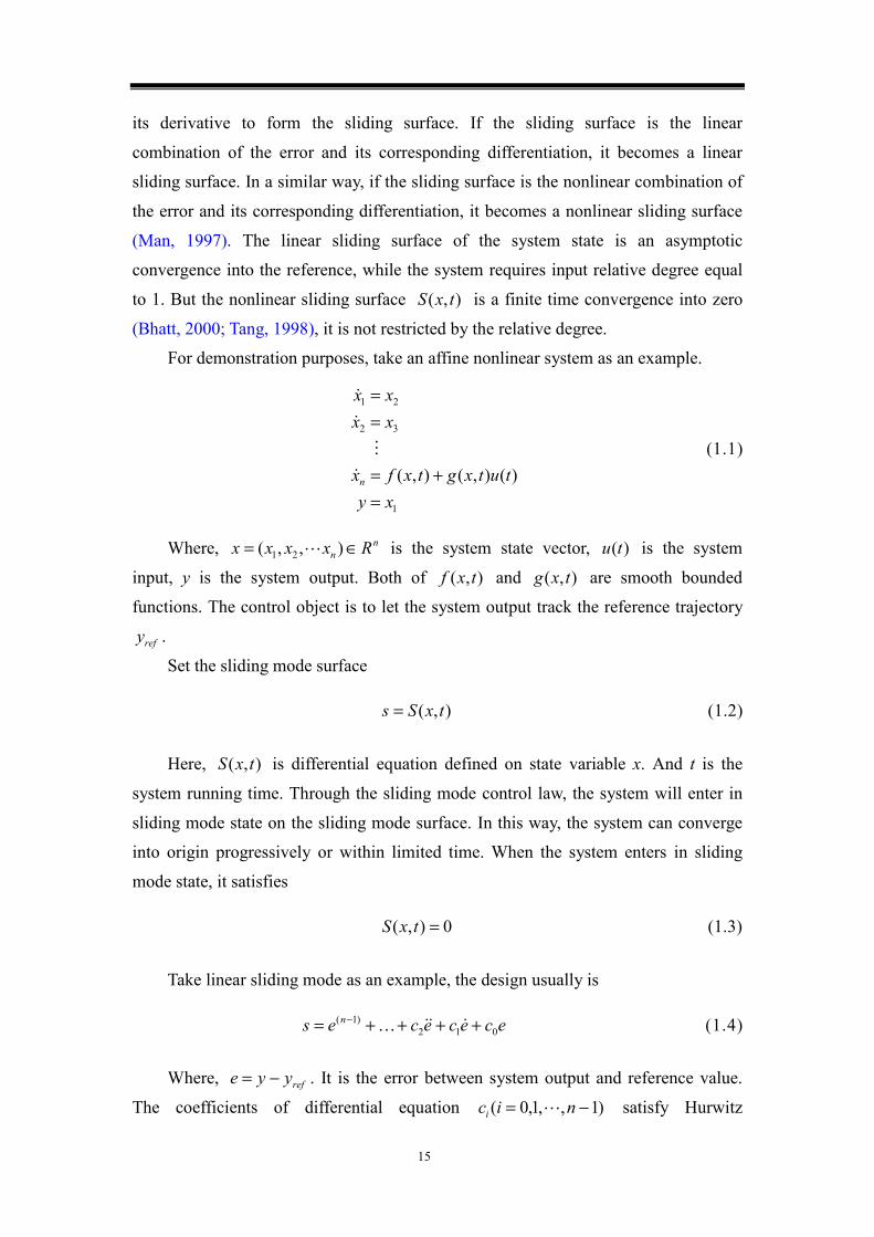
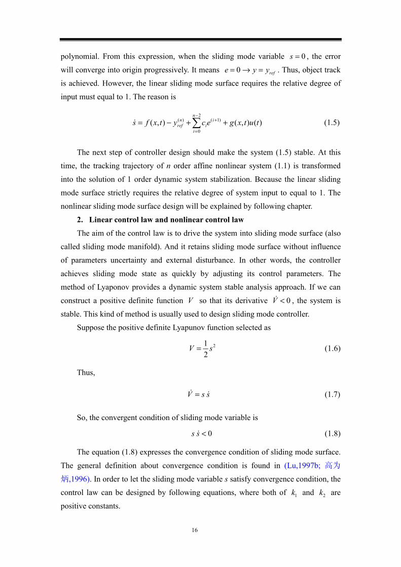
and 0)0(2 =x . Then, the phase plane of system is shown in figure 1-2. If we amplify
the partial sliding mode surface 0=s , the figure 1-3 displays the chattering.
-0.2 0 0.2 0.4 0.6 0.8 1 1.2-1
-0.8
-0.6
-0.4
-0.2
0
0.2
x1
x 2
0.08 0.082 0.084 0.086 0.088 0.09 0.092 0.094 0.096 0.098 0.1-0.096
-0.094
-0.092
-0.09
-0.088
-0.086
-0.084
-0.082
x1
x 2
Fig. 1-2 Phase plane of second order system Fig. 1-3 Partial enlarged drawing SM surface
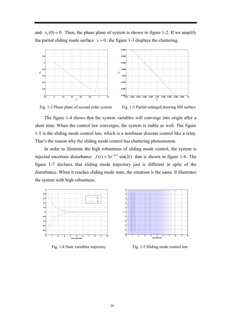
The figure 1-4 shows that the system variables will converge into origin after a
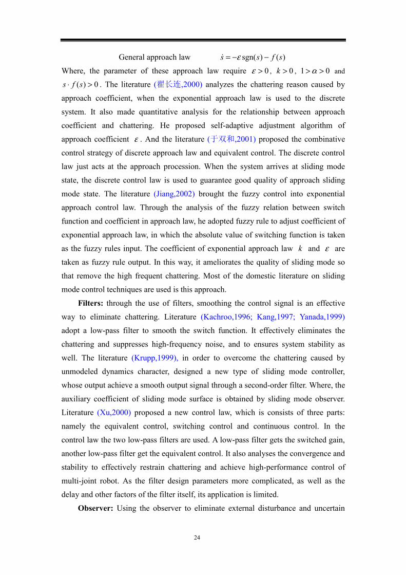
short time. When the control law converges, the system is stable as well. The figure
1-5 is the sliding mode control law, which is a nonlinear discrete control like a relay.
That’s the reason why the sliding mode control has chattering phenomenon.
In order to illustrate the high robustness of sliding mode control, the system is
injected uncertain disturbance )2sin(5)( 2.0 tetf t−= that is shown in figure 1-6. The
figure 1-7 declares that sliding mode trajectory just is different in spite of the
disturbance. When it reaches sliding mode state, the situation is the same. It illustrates
the system with high robustness.
0 1 2 3 4 5 6 7 8 9 10-1
-0.8
-0.6
-0.4
-0.2
0
0.2
0.4
0.6
0.8
1
time (second)
x1
x2
0 1 2 3 4 5 6 7 8 9 10-5
-4
-3
-2
-1
0
1
2
3
4
5
time (s)econd
u
Fig. 1-4 State variables trajectory Fig. 1-5 Sliding mode control law

21
0 1 2 3 4 5 6 7 8 9 10-4
-3
-2
-1
0
1
2
3
4
5
tiem (second)
f(t)
-0.2 0 0.2 0.4 0.6 0.8 1 1.2
-0.8
-0.6
-0.4
-0.2
0
0.2
0.4
x1
x 2
wihtout disturbance
with disturbance
2x
1x Fig. 1-6 Uncertainty bounded disturbance Fig. 1-7 System phase plane with disturbance
1.3.3 Chattering problem and solving
The sliding mode control actually is the structure of feedback controller occur
changes according to certain rules when the system state passes across the different
regions in state space. It makes the control systems has a certain adaptive ability to the
internal parameter variations and external disturbance so that the system performance
achieves the desired targets. However, due to the sliding mode control law with a
discrete switch control, it has chattering. Moreover, the ideal switching frequency of
sliding mode control is infinity, which can not be realized in the actual system. In
addition, in practical applications, the switch with time-delay, discontinuous sampling,
system inertia, and even the error of state measurement will cause the chattering
phenomenon in sliding mode control. In this way, the sliding mode control system is
equivalent to high gain system accompanied by high frequency jitter, which could
bring a very harmful consequence for control systems.
Therefore, the chattering phenomenon has become the biggest developing
obstacle of sliding mode control technology. The academics have continued to
weaken or prevent the chattering without interruption. In order to reduce or eliminate
chattering, a large number of researchers have put a lot of hard work in their
respective areas of research. To sum up, it is mainly in the following several ways.
Pseudo-sliding mode: to reduce the chattering, the first thought is to improve
the control law to weaken the impact of chattering. Literature (Slotine,1983)
introduced a concept of "pseudo-sliding mode" and the "boundary layer". It adopted
saturation function ),( δssat instead of sign function )sgn(s to realize the sliding
mode control.

22
0 ||/||)sgn(
),( >⎩⎨⎧
≤>
= δδδδ
δsifssifs
ssat
Outside the boundary layer, it uses switch sliding mode control. Otherwise, inside the
boundary layer, it uses continuous state feedback control. In this way, it reduces the
chattering, but loses the finite time convergence. The figure 1-8 is the saturation
function and sign function.
Fig. 1-8 sign function )sgn(s and saturation function ),( δssat
After that, many scholars start to study the switch function and boundary layer. Some
of them propose serialization of unit vector.
δ
δ+
=||
),(s
sksu (1.23)
Some literature calls it signum-like function. Where, the choose of δ can guarantee
precision. Besides, there is power law interpolation.
⎪⎩
⎪⎨
⎧∈
=≤<>
= − )1,0[ 00||0)sgn()||(||)sgn(
),( )1( qs
sssksifsk
su q δδδ
δ (1.24)
In addition, there are arc tangent function )(tan),( 1 δδ sksu −⋅= , hyperbolic curve
)tanh(),( δδ ssu = and etc. instead of original switch function )sgn(s . Their aim is
to reduce or remove the chattering. The various approximate functions are shown in
figure 1-9.

23
Fig. 1-9 Approximated function effect schematic plan
The smaller the boundary layer, the control effect will be better. But, at the same time,
this will enlarger the control gain and chattering enhancement; On the contrary, the
greater the boundary layer, the chattering will be smaller. But they will decrease the
control gain, and the effect of control become worse. In fact, this approximate sliding
mode control is the balance between the system performance and robustness.
Approach law: Prof. Gao Weibing proposed approach law (高为炳,1996) in
1989. Take the exponential approach law ksss −−= )sgn(ε as an example, through
the adjustment of parameter k and ε , it can not only guarantee the dynamic quality
of sliding mode arrival procession, but also weaken high frequent chattering of
control signal. But if the ε is too great, it will result in chattering. The approach law
is used to study dynamic quality of arrival procession, when the system converges
from the any initialization within limited time. According to the different system, we
can design the various approach law, such as
Uniform approach law )sgn(ss ε−=
Power approach law )sgn(|| ssks α−=
Exponential approach law ksss −−= )sgn(ε
24
General approach law )()sgn( sfss −−= ε
Where, the parameter of these approach law require 0>ε , 0>k , 01 >>α and
0)( >⋅ sfs . The literature (翟长连,2000) analyzes the chattering reason caused by
approach coefficient, when the exponential approach law is used to the discrete
system. It also made quantitative analysis for the relationship between approach
coefficient and chattering. He proposed self-adaptive adjustment algorithm of
approach coefficient ε . And the literature (于双和,2001) proposed the combinative
control strategy of discrete approach law and equivalent control. The discrete control
law just acts at the approach procession. When the system arrives at sliding mode
state, the discrete control law is used to guarantee good quality of approach sliding
mode state. The literature (Jiang,2002) brought the fuzzy control into exponential
approach control law. Through the analysis of the fuzzy relation between switch
function and coefficient in approach law, he adopted fuzzy rule to adjust coefficient of
exponential approach law, in which the absolute value of switching function is taken
as the fuzzy rules input. The coefficient of exponential approach law k and ε are
taken as fuzzy rule output. In this way, it ameliorates the quality of sliding mode so
that remove the high frequent chattering. Most of the domestic literature on sliding
mode control techniques are used is this approach.
Filters: through the use of filters, smoothing the control signal is an effective
way to eliminate chattering. Literature (Kachroo,1996; Kang,1997; Yanada,1999)
adopt a low-pass filter to smooth the switch function. It effectively eliminates the
chattering and suppresses high-frequency noise, and to ensures system stability as
well. The literature (Krupp,1999), in order to overcome the chattering caused by
unmodeled dynamics character, designed a new type of sliding mode controller,
whose output achieve a smooth output signal through a second-order filter. Where, the
auxiliary coefficient of sliding mode surface is obtained by sliding mode observer.
Literature (Xu,2000) proposed a new control law, which is consists of three parts:
namely the equivalent control, switching control and continuous control. In the
control law the two low-pass filters are used. A low-pass filter gets the switched gain,
another low-pass filter get the equivalent control. It also analyses the convergence and
stability to effectively restrain chattering and achieve high-performance control of
multi-joint robot. As the filter design parameters more complicated, as well as the
delay and other factors of the filter itself, its application is limited.
Observer: Using the observer to eliminate external disturbance and uncertain
25
items has become a study to solve the chattering problem. The literature (Kawamura,
1994) designed a new type observer of disturbance. Through feedforward
compensation for the external perturbation injected, it greatly reduced switching gain
of sliding mode controller, and effectively eliminated the chattering. Y. S. Kim
designed a disturbance observer based on binary control theory. In this paper, the
disturbance observed was used for feedforward compensation to reduce the chattering.
(Kin,1996). In addition, the literature (Edwards,2004) designed a sliding mode
observer to achieve a fault detection and fault-tolerant control.
Neural Sliding: neural network is a nonlinear continuous time dynamic system.
It has a very strong self-learning function and a powerful mapping ability for
nonlinear systems. The neural networks used for the sliding mode control, can reduce
the chattering. The literature (Morioka,1995) used neural network to estimate the
uncertainty and unknown external disturbance, and achieve the equivalent control
based on neural network. It effectively eliminated the chattering as well. The literature
(Ertugrul,2000) proposed a new type neural network method of sliding mode control,
using two neural networks to approach equivalent control and switch control of
sliding mode control respectively without the object model. It effectively eliminates
the chattering, which has been successfully applied to robot trajectory tracking. The
literature (Huang,2003) used the approximation capability of neural networks,
designed a sliding mode controller based RBF neural network. It will take the switch
function as network input. And the controller is realized entirely by continuous RBF
function, which eliminates the switching chattering. In the literature (Da,2000), the
sliding mode controller is divided into two parts. One part is for the neural network
sliding mode controller, the other part is a linear feedback controller. Using fuzzy
neural network sliding mode control to replace the output of the switching function, it
ensures the continuity of the control law, essentially eliminates the chattering.
Fuzzy sliding mode: According to experience, the fuzzy rules design can
effectively reduce the chattering in sliding mode control. Fuzzy sliding mode control
often the control signals, change the discontinuous control signals to continuous one.
It can reduce or avoid the chattering of sliding mode control. The fuzzy logic sliding
mode control can achieve parameters self-adjusting. The input of fuzzy control is not
),( ee but ),( ss . Through the design of fuzzy rule, it drives sliding mode surface to
zero, so that remove the switching part of the sliding mode control. Literature (Ha,
2001) used the equivalent control, switching control and fuzzy control constituting the

26
fuzzy sliding mode controller. In the fuzzy controller, the design of fuzzy rules
reduces the impact of the switching control, effectively eliminates the chattering.
Literature (Zhuang,2000) took the use of fuzzy control system to estimate the
uncertainty items online, achieving fuzzy switching gain self-adjust. It guarantees the
sliding mode to reach the condition satisfied as far as reducing the switching gain.
Literature (Ryu,2001) established the chattering indicators of sliding mode control in
order to reduce chattering to design fuzzy rules. The fuzzy rules, input indicators for
the current chattering size of the output of fuzzy rules for the boundary layer thickness,
through the fuzzy reasoning, realize the adaptive adjustment of boundary layer
thickness. Literature (张天平,1995) proposed a fuzzy logic based on continuous
sliding mode control method, using continuous fuzzy logic switch instead of
non-continuous sliding mode control to avoid chattering.
Higher-order sliding-mode: the high order sliding mode control is a new
method proposed in last decade (Levant,1993). The switch function in traditional
sliding mode control is generally dependent on the system state, has nothing to do
with the control input. Discontinuous items will be directly transferred to the
controller. But, the high order sliding mode control constitutes a new sliding mode
surface using the sliding mode control variable and its differentiations, transfers the
discrete items to the first order or higher order derivative of sliding mode variable.
That is expressed by }0{ )1( ===== −rsssS . It should be clear is that when the
differential order of sliding mode variables equals to 2, it is called the second order
sliding mode control in some reference (Koshkouei,2005;晁红敏,2001;吴玉香,2006).
Sometimes, it also is known as dynamic sliding mode control (dynamic sliding mode ,
DSM). Literature (Bartolini,1998; Bartolini,2001) through the design of the second
order derivative of sliding mode variable, it achieves to sliding mode control without
chattering in the un-modeled dynamics and uncertain systems. And the method is
extended to multiple-input multiple-output system. The high order sliding mode
controller has the advantage of simple design, easy to implement, without precise
mathematical models. It can effectively eliminate the chattering and improve the
convergence precision as well.
Using high order sliding mode control, it not only eliminates the chattering
problems that exist in the traditional sliding mode, but also avoids the requirements of
relative degree that must be equal to 1 in the control law design. In this paper, after
the analysis and comparison of several sliding mode control techniques, high order
27
sliding mode control is mainly used to eliminate chattering, implement model
uncertain robust control for nonlinear systems. The thesis also focuses on multi-input
multi-output nonlinear systems robust decoupling control.
1.4 The application and research of nonlinear sliding mode control systems
The sliding mode control system has strong robustness to the uncertainties in the
system. Therefore, there is a great deal of applied research on sliding mode control
theory in aviation, aerospace, electrical motor and power systems, robotics and
industrial control (Shtessel,1996; Galzi,2007; Laghrouche,2003).
Actually, the sliding mode control of nonlinear systems in the industry control
field has received considerable attention. In the initial stage of variable structure, it’s
mainly applied to the field of industry control. With the development of industrial
technologies, the requirements of control precision and robustness to multi-variable,
nonlinear practical equipments has gradually increased day by day and the application
of sliding mode control in the industry control field has prompted step by step
(Corradini,2000; Kim,2004; Rios-Gastelum, 2003). For the first time in 1983, the
sliding mode control was applied into robot control by Slotine, who designed the
sliding mode controller of time-varying referring trajectory. Subsequently, he
combined the sliding mode control and the feedback linearization technique to extend
research results to the sliding mode controller design of more general rigid-body robot
and to achieve the referring trajectory tracking control. Yeh studied the sliding mode
tracking control of satellites (Yeh,2000). Calise learned the robust sliding mode
control of helicopter movement system with uncertain nonlinear system. Lu X.Y.
designed trajectory tracking robust controller for the control problem of large aircraft
from aerospace controller (Lu,1997). Y.B. Shtessel used robust sliding mode control
to achieve the missile guidance control and wing flight control of F18 (Shtessel,2007).
Toumes achieved a high altitude rocket navigation control. McDuffie designed
decoupled sliding mode observer for satellite attitude control (McDuffie,1997). These
controllers must be strong robustness to the system parameter variations and external
disturbances. In recent years, the sliding mode control for nonlinear systems has been
widespread paid much attention and become a research hot spot.
There are so many characteristics for permanent magnet synchronous motor such
as compact structure, high power density, high air-gap flux and high-torque inertia
ratio, which in the servo system has been widely used. But the permanent magnet
28
synchronous motor is a nonlinear system, which includes the product term of angular
velocity and d-q axis electric current, it must achieve decoupling and linearization of
the system to get the accurate control performance. So, the feedback linearization in
nonlinear control theory can transform nonlinear systems into linear systems
(Bodson,1993). However, the parameters in motor dynamic model will be affected by
the complex environment and the effect is still changing. Accordingly, the robust
control has become an effective way to improve performances. M. Kadjoudj designed
a high performance permanent magnet synchronous motor with an adaptive fuzzy
controller (Kadjoudj,2001). J. Xu designed a robust adaptive stepping controller to
improve motor performance (J. Xu,1998). S. Laghrouche adopted second order
sliding mode control to design a nonlinear robustness controller for permanent magnet
synchronous motor (Laghrouche,2004). These high performance robust controllers in
synchronous motors have been very successful in the application. But because
permanent magnet motor is affected by external influences and its own changing
parameters and many other factors, there are still many issues worth studying, such as
motor parameter identification, state estimation, perturbation estimation and so on.
The requirements in the applications to the control performance point out the
direction for further study of sliding mode control theory and should be of great
significance to the development of sliding mode control. As there are a large number
of nonlinear problems in engineering, approximate linear model can not describe the
dynamic characteristics of the system. In the real production, because of the
environment in which a number of nonlinear controlled objects work is very complex,
many internal uncertainties and external disturbance affect the control systems.
Therefore, the robust control of uncertain system is an important research area in
nonlinear sliding mode control.
1.5 The main research contents of the paper
Based on the research of the current sliding mode control theory applied to
nonlinear systems, it chiefly launches an in-depth study and exploration in allusion to
several facing issues of nonlinear sliding mode control theory and gives the
corresponding research findings and results.
1. The thesis shows the research background and systematically introduces the
history and the current development situation of nonlinear control and sliding mode
control theory. At the same time, it describes the control superior advantages of their

29
combination. Meanwhile, it analyzes the problems in the current sliding mode control
and sum up various research directions to overcome the chattering. On this basis, it
illustrates the study significance of the topic.
2. It introduces the basic theory of differential geometry as well as the latest
research results of exact feedback linearization field in detail. The decoupling control
of nonlinear MIMO system has always been a critical study of nonlinear problems. In
sequence, decoupling controllers are designed for each nonlinear system. Through
simulation study, it has established a basic theoretical research for further application
of multi-variable complex systems.
3. As the chattering phenomenon which exists in the traditional sliding mode
controller is extremely negative to industrial control, adopting high order sliding
mode control algorithm can not only guarantee the control precision but also eliminate
the chatters. Besides, it uses simulation experiments to demonstrate the validity of
research results.
4. In the controller design, we frequently encounter the problem of solving
variables’ different order differentiations. But the traditional numerical method needs
a large quantity of calculation and its accuracy level is not high. We study the sliding
mode differentiator which uses high order sliding mode algorithm to achieve the
variable derivative of arbitrary order. In engineering, the differentiator with strong
robustness and high accuracy can not only greatly simplify the calculation of the
workload but also ensure the calculation accuracy. At last, the paper designs a precise
sliding mode differentiator and carries out application simulation research for MIMO
nonlinear systems.
5. It takes research results of the sliding mode control for nonlinear systems
studied to apply to servo system of the MIMO permanent magnet synchronous motor
system, and combines the multi-variable nonlinear decoupling control and recent
studied high order sliding mode control with strong robustness. In addition, it designs
the robust sliding mode controller for the system under the parameters uncertain and
external torque disturbance, in order to improve the performances of the motor.
Meanwhile, for several current research focused on synchronous motor, it uses high
order sliding mode control and its differential algorithm to achieve the items of state
estimation, parameter identification and disturbance torque estimation for permanent
magnet synchronous motor.
6. Finally, through real-time physical control platform dSPACE, it makes the

30
physical verification to robust sliding mode servo driving control MIMO system of
the permanent magnet synchronous motor, in order to validate the consistency of
experimental and theoretical research.

31
Chapter 2 Nonlinear system high order sliding mode control
In the introduction of first chapter, we have known the sliding mode control with
the strong robustness for the internal parameters and external disturbances. In addition,
the appropriate sliding surface can be selected to reduce order for control system.
However, due to the chattering phenomena of sliding mode control, the high
frequency oscillation of control system brings challenge for the application of sliding
mode control. On the other hand, the choice of sliding surface strictly requires system
relative degree to equal to 1, which limits the choice of sliding surface.
In order to solve the above problems, the introduction of first chapter also
illustrates the current developments and research methods in this field. This chapter
focuses on a new type of sliding mode control, that is, higher order sliding mode
control. The technology not only retains advantage of strong robustness in the
traditional sliding mode control, but also enables discontinuous item variables
transmit into the first order or higher order sliding mode derivative to eliminate the
chattering. Besides, the design of the controller no longer must require relative degree
to be 1. Therefore, it is greatly simplified to design parameters of sliding mode
surface.
Emelyanov and others first time propose the concept of high order differentiation
of sliding mode variable, but also provide a second order sliding mode twisting
algorithm, and prove its convergence (Emelyanov,1996). Another algorithm is super
twisting, which can completely eliminate chattering (Emelyanov,1990), although the
relative degree of sliding mode variable is required to equal to 1. In the second order
sliding mode control, Levant proved sliding mode accuracy is proportional to )( 2τo
the square of the switching delay time. It has also become one of the merits of high
order sliding mode control (Levant,1993). Since then, the high order sliding mode
controller has been developed and applied rapidly. For example, Bartolini and others
propose a second order sliding mode control applied the sub-optimal algorithm
(Bartolini,1997; Bartolini,1999). After the concept of high order sliding mode control
was applied to bound operator in (Bartolini,2000). Levant used high order sliding
mode control in aircraft pitch control (Levant,2000) as well as the exact robust
differentiator (Levant,1998). About the summary of high order sliding mode control is
also described in the literature (Fridman,2002).
This chapter is structured as follows: 2.1, introduce a second order sliding mode
32
control that eliminate the chattering essentially; 2.2, Give simulation examples of the
actual system against the algorithm of 2.1; 2.3, Introduce the algorithm arbitrary order
sliding model control in detail; 2.4, Take simulation research to the algorithm of 2.3;
2.5, Give a quasi-continuous high order sliding mode control algorithm so that state
variable can be more smooth; 2.6, Summary of this chapter.
2.1 Second order sliding mode control
Strictly speaking, second order sliding mode control is a special kind of high
order sliding mode control actually. But, in the design of the controller, the highest
order of sliding mode variable is 2, so called second order sliding mode control
(SOSM). Some literatures also call it as the dynamic sliding mode control (DSM).
Without losing generality, considering a state equation of single input nonlinear
system as
),(
)()(txsy
uxgxfx=
+= (2.1)
Where, nRx∈ is system state variable, t is time, y is output, u is control
input. Here, )(xf , )(xg and )(xs are smooth function. The control objective is
making output function 0≡s .
Differentiate the output variables continuously, we can get every order derivative
of s . According to the conception of system relative degree, there are two conditions.
I. Relative degree 1=r ,if and only if 0≠∂∂ su
II. Relative degree 2≥r ,if )1,2,1( 0)( −==∂∂ risu
i ,and 0)( ≠∂∂ rsu
If the relative degree 1=r , traditional sliding mode control can be used to
design controller. Else, it needs to design a second order sliding mode controller.
Second order sliding mode control is able to eliminate chattering.
Suppose system relative degree equals 1, differentiate sliding mode variable
twice continuously, then
])()()[,(),( uxgxftxsx
txst
s +∂∂+
∂∂= (2.2)
33
uxx
utxsu
uxgxftxsx
txst
s
xx
)()(
),(])()()[,(),(
)()(
γϕγϕ
+=
∂∂++
∂∂+
∂∂=
(2.3)
In order to achieve this aim of eliminating chattering, the u derivative of
control input u is made as actual control variable. The discontinuous control law u
will drive sliding mode variable 0=s in the second order sliding mode surface 2S .
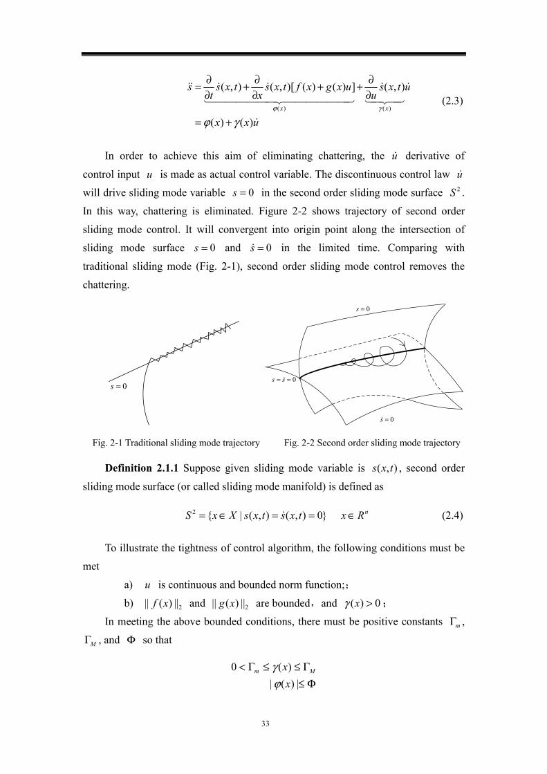
In this way, chattering is eliminated. Figure 2-2 shows trajectory of second order
sliding mode control. It will convergent into origin point along the intersection of
sliding mode surface 0=s and 0=s in the limited time. Comparing with
traditional sliding mode (Fig. 2-1), second order sliding mode control removes the
chattering.
0=s
0=s
0=s
0== ss
Fig. 2-1 Traditional sliding mode trajectory Fig. 2-2 Second order sliding mode trajectory
Definition 2.1.1 Suppose given sliding mode variable is ),( txs , second order
sliding mode surface (or called sliding mode manifold) is defined as
}0),(),(|{2 ==∈= txstxsXxS nRx∈ (2.4)
To illustrate the tightness of control algorithm, the following conditions must be
met
a) u is continuous and bounded norm function;;
b) 2||)(|| xf and 2||)(|| xg are bounded,and 0)( >xγ ;
In meeting the above bounded conditions, there must be positive constants mΓ ,
MΓ , and Φ so that
Φ≤Γ≤≤Γ<
|)(|)(0x
x Mm
ϕγ
34
Here are some of the control algorithms to make the dynamic system (2.3)
stability. And they ensure that the second order sliding mode convergence in finite
time.
Twisting algorithm:
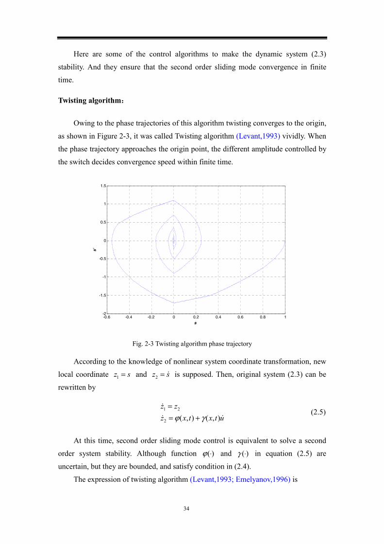
Owing to the phase trajectories of this algorithm twisting converges to the origin,
as shown in Figure 2-3, it was called Twisting algorithm (Levant,1993) vividly. When
the phase trajectory approaches the origin point, the different amplitude controlled by
the switch decides convergence speed within finite time.
-0.6 -0.4 -0.2 0 0.2 0.4 0.6 0.8 1-2
-1.5
-1
-0.5
0
0.5
1
1.5
s
s'
Fig. 2-3 Twisting algorithm phase trajectory
According to the knowledge of nonlinear system coordinate transformation, new
local coordinate sz =1 and sz =2 is supposed. Then, original system (2.3) can be
rewritten by
utxtxz
zz),(),(2
21
γϕ +==
(2.5)
At this time, second order sliding mode control is equivalent to solve a second
order system stability. Although function )(⋅ϕ and )(⋅γ in equation (2.5) are
uncertain, but they are bounded, and satisfy condition in (2.4).
The expression of twisting algorithm (Levant,1993; Emelyanov,1996) is
35
0
0
0
||,0||,0
||
)sgn()sgn(
uussuuss
uu
sVsV
uu
M
m
<≤<>
>
⎪⎩
⎪⎨
⎧
−−
−= (2.6)
Where, 0u , mV and MV are positive constant. The sufficient condition of
sliding mode surface convergence within limited time is
Φ+Γ>Φ−Γ
>ΓΦΓ>
mMMm
mM
mMm
VVVV
sV ),4max( 0
(2.7)
Similarly, if the system relative degree is 2, the control algorithm is
⎩⎨⎧
>≤
−−
=00
)sgn()sgn(
ssss
sVsV
uM
m (2.8)
Super twisting algorithm:
The phase trajectory of super twisting algorithm is shown in figure 2-4. It is also
twisting convergent to origin, which is similar with twisting algorithm. But only its
control algorithm is continuous. Control input u is composed by two parts
(Levant,1993). One is differentiation of discontinuous item. The other is continuous
functions of sliding mode variable. The expression is
0
002
1
21
||||
)sgn(||)sgn(||
)(
1||1||
)sgn(
)(
)()()(
ssss
ssss
tu
uu
sWu
tu
tututu
≤>
⎩⎨⎧
−−
=
⎩⎨⎧
≤>
−−
=
+=
ρ
ρ
λλ
(2.9)
Where, W , λ , 0s and ρ are positive constant. The sufficient condition of
second order sliding mode surface convergence within limited time is
5.00)()(4
22
≤<Φ−ΓΦ+Γ
ΓΦ≥
ΓΦ>
ρ
λWW
W
m
M
m
m
(2.10)
From the equation (2.9), we can see that this algorithm need not differentiate

36
sliding mode variable. In addition, if 1=ρ , super twisting algorithm is convergent to
origin exponentially. At the moment, control input u hasn’t requirement of bound.
When ∞=0s , Algorithm can be simplified as
)sgn(
)sgn(||
1
1
sWuussu
−=+−= ρλ
(2.11)
-1 -0.5 0 0.5 1 1.5 2-5
-4
-3
-2
-1
0
1
2
3
s
s'
Fig. 2-4 Super Twisting algorithm phase trajectory
From the results of second order sliding mode control algorithm, the design
object of controller u is to make }0),(),(|{2 ==∈= txstxsXxS in second order
sliding mode surface.
2.2 Simulation example (levant,2003)
Considering a single input single output nonlinear dynamic system of
double-wheel drive motion robot (figure 2-5), the mathematic model is
ulvvyvx
=
=
==
θ
θϕ
ϕϕ
tan
sin cos
(2.12)
Where, x and y are Cartesian coordinate, ϕ is orientation angle, v is
forward velocity, l is the length of two axle, θ is drive angle.

37
It is known that smv /10= and ml 5= . The trajectory tracked is
5)05.0sin(10)( += xxd . The initial value of state is 0)0()0()0()0( ==== θϕyx .
The control aim is to drive robot tracking given trajectory )(xdy = from the
initial position. So choosing the sliding mode variable )(xdys −= , according to the
principle of sliding mode control, it achieve the control aim when the sliding mode
variable converge into origin ( 0=s ) finally. However, in the second order sliding
mode, the control law requires the relative degree of sliding mode variable to equal 1.
Obviously, the relative degree of )(xdys −= doesn’t equal 1. So, under the
requirement of relative degree, the Hurwitz polynomial should be structured. That is
zzzzzP nn
n01
)1(1
)()( λλλ ++++= −− , the parameters )10( −≤≤ niiλ are positive
constant.
ϕ
θ
x
y
l
Fig. 2-5 Double drive motive robot model
Thus, the sliding surface satisfying relative degree can be redesigned as
))(())(()( 01 xdyxdyxdys −+−+−= λλ (2.13)
Differentiate sliding mode variable s , then
))(())(()( 01 xdyxdyxdys −+−+−= λλ (2.14)
Take the numerical calculation into (2.14), then
)cos)05.0cos(5sin10()tansin)05.0cos(10 cos)05.0sin(5.2tancos20(
secsin)05.0cos(10tancos)05.0cos(20 tansincos)05.0sin(5tansin)05.0sin(10 cos)05.0cos(25.1seccos20tansin40
0
21
22
322
ϕϕλθϕϕθϕλ
θϕθϕθϕϕθϕϕθϕθϕ
⋅−+⋅⋅+⋅+⋅+
⋅⋅⋅+⋅⋅+
⋅⋅⋅−⋅⋅−⋅+⋅⋅+⋅−=
xxx
uxxxx
xus
(2.15)

38
From the equation (2.15) we can see that the control input u first time appears
in the first order derivative of sliding mode variable s . That means the relative
degree of sliding mode variable to control input is 1. At the moment, according to the
twisting algorithm, controller u can be designed. Here, u is obtained by integral of
u . The value of the parameters mV and MV are smaller, the convergence time is longer.
But the value of the parameters mV and MV are greater, the chattering is more obvious.
Thus, the parameters in this controller are 10=mV and 30=MV . In addition, the
coefficient of Hurwitz polynomial are 21 =λ and 10 =λ . The track trajectory curve
of system is shown in figure 2-6.
0 20 40 60 80 100 120 140 160 180-10
-5
0
5
10
15
20
x
y
y
g(x)
Fig. 2-6 Track trajectory curve
From the figure 2-6 we can see that system dynamic effectiveness is good. After
a limited time, second order sliding mode control law converges into origin to
guarantee system track effectiveness. The figure 2-7 is convergence trajectory of
sliding mode variable within limited time. The system converges into origin at the
0.5s, at that time, for the control system 0)( =−= xdys . It achieve dynamic track of
given trajectory.
Figure 2-7 also shows that second order sliding mode control transfer chattering
to a higher order sliding mode surface. It is the biggest difference with the traditional
sliding mode control. Therefore, first order (or lower order) sliding surface become
smooth. So, the second order sliding mode control eliminates the impact of the
chattering essentially. But also precisely because of this reason, a strong impetus to
the second order sliding mode control and high order sliding mode control are greatly
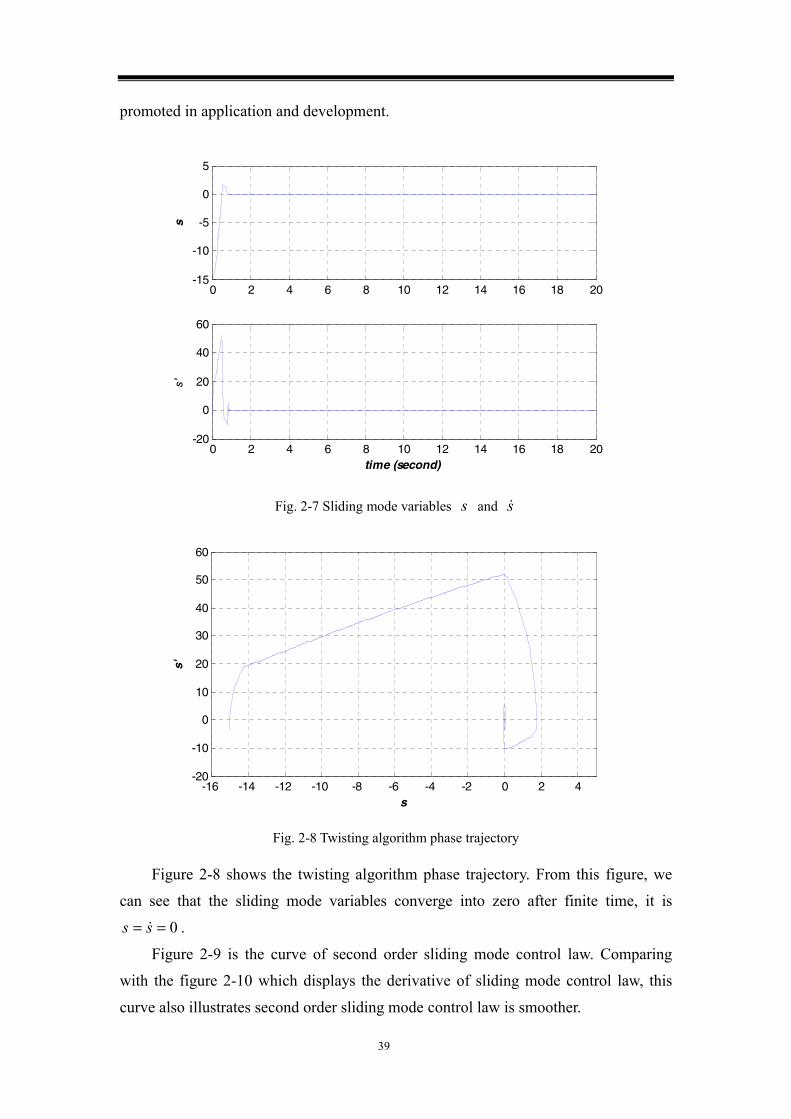
39
promoted in application and development.
0 2 4 6 8 10 12 14 16 18 20-15
-10
-5
0
5s
0 2 4 6 8 10 12 14 16 18 20-20
0
20
40
60
time (second)
s'
Fig. 2-7 Sliding mode variables s and s
-16 -14 -12 -10 -8 -6 -4 -2 0 2 4-20
-10
0
10
20
30
40
50
60
s
s'
Fig. 2-8 Twisting algorithm phase trajectory
Figure 2-8 shows the twisting algorithm phase trajectory. From this figure, we
can see that the sliding mode variables converge into zero after finite time, it is
0== ss .
Figure 2-9 is the curve of second order sliding mode control law. Comparing
with the figure 2-10 which displays the derivative of sliding mode control law, this
curve also illustrates second order sliding mode control law is smoother.

40
0 2 4 6 8 10 12 14 16 18 20-1.5
-1
-0.5
0
0.5
1
1.5
time (second)
con
tro
l la
w u
Fig. 2-9 Control law curve
0 2 4 6 8 10 12 14 16 18 20-40
-30
-20
-10
0
10
20
30
40
time (second)
con
tro
l la
w u
'
Fig. 2-10 Control law derivative curve
It should be noted that, the regulation of the system controller parameters (also
including a Hurwitz polynomial parameters) is actually not very easy. It need repeat
several times in order to meet the requirements of control. But in the actual system
applications, because of too many parameters to adjust and match, the problem
becomes more difficult. The following section will introduce an arbitrary order sliding
mode control to avoid the strict condition requirements of the relative degree equal to
1. In this case, the relative degree can be arbitrary values. So the corresponding
controller can be designed so as no longer afraid of suitable Hurwitz polynomial

41
parameters. And it greatly simplifies the design process and the application.
Here, we should give a summary. Besides the super-twisting and twisting
algorithm, second order sliding mode control law has many else control law algorithm.
In this field, many scholars have invested in a substantial amount of research. For
example, in some literatures (Bartolini,1998; Bartolini,1998b; Bartolini,1998c) also
introduced the Sub-optimal algorithm, the literature (Emelyanov,1986;Levant,1993)
introduced the Drift algorithm, and so on.
2.3 Arbitrary order sliding mode control
Second order sliding mode control takes the use of the differential role of control
law in the second order sliding surface, within the limited time to convergence, and to
eliminate the chattering in the first order sliding mode surface. However, the second
order sliding mode control algorithm requires the relative degree of system to equal to
1. If the relative degree of system is 2 or more, is there a general algorithm for it?
Fortunately, the answer to this question is yes.
In recent years, because arbitrary order sliding mode control technique not only
retains the traditional sliding mode control simple structure with strong robustness,
but also eliminates the chattering phenomenon in the traditional sliding mode, at the
same time, gets rid of the constraints of system relative degree. Therefore theoretical
research and engineering applications has caused widespread concern and has been
constant development. In arbitrary order sliding mode control, its core idea is the
discrete function acts on a higher order sliding mode surface, making
0),(),(),(),( )1( ==== − txstxstxstxs r (2.16)
Suppose the relative degree of system (2.1) equals to r , generally speaking,
when the control input u first time appears in r -order derivative of s , that is
0)( ≠duds r , then we take r -order derivative of s for the output of system (2.1), )1(,,, −rssss can be obtained. They are continuous function for all the x and t .
However, corresponding discrete control law u acts on )(rs . Selecting a new local
coordinate, then
),,(),,( )1(21
−== rr sssyyyy (2.17)
So,
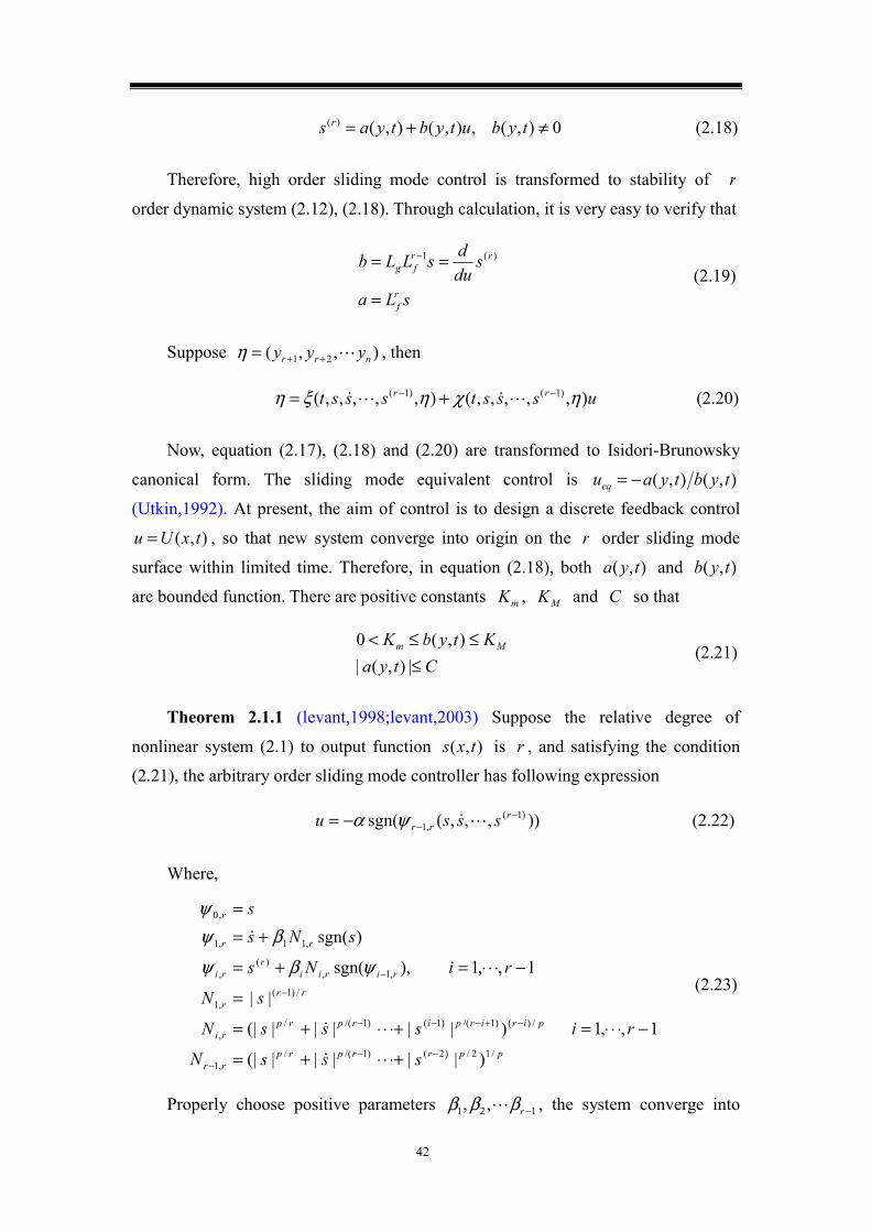
42
0),( ,),(),()( ≠+= tybutybtyas r (2.18)
Therefore, high order sliding mode control is transformed to stability of r
order dynamic system (2.12), (2.18). Through calculation, it is very easy to verify that
sLa
sdudsLLb
rf
rrfg
=
== − )(1
(2.19)
Suppose ),,( 21 nrr yyy ++=η , then
ussstssst rr ),,,,,(),,,,,( )1()1( ηχηξη −− += (2.20)
Now, equation (2.17), (2.18) and (2.20) are transformed to Isidori-Brunowsky
canonical form. The sliding mode equivalent control is ),(),( tybtyaueq −=
(Utkin,1992). At present, the aim of control is to design a discrete feedback control
),( txUu = , so that new system converge into origin on the r order sliding mode
surface within limited time. Therefore, in equation (2.18), both ),( tya and ),( tyb
are bounded function. There are positive constants mK , MK and C so that
Ctya
KtybK Mm
≤≤≤<
|),(|),(0
(2.21)
Theorem 2.1.1 (levant,1998;levant,2003) Suppose the relative degree of
nonlinear system (2.1) to output function ),( txs is r , and satisfying the condition
(2.21), the arbitrary order sliding mode controller has following expression
)),,,(sgn( )1(,1
−−−= r
rr sssu ψα (2.22)
Where,
pprrprprr
pirirpirprpri
rrr
ririir
ri
rr
r
sssN
risssN
sN
riNs
sNss
/12/)2()1/(/,1
/)()1/()1()1/(/,
/)1(,1
,1,)(
,
,11,1
,0
)|||||(|
1,,1 )|||||(|
||
1,,1 ),sgn(
)sgn(
−−−
−+−−−
−
−
⋅+⋅⋅+=
−⋅⋅⋅=⋅+⋅⋅+=
=
−⋅⋅⋅=+=
+==
ψβψ
βψψ
(2.23)
Properly choose positive parameters 121 ,, −rβββ , the system converge into

43
origin on the r order sliding mode surface within limited time. Finally, when 0≡s ,
it achieves control object.
The choice of positive parameters 121 ,, −rβββ is not unique. Here, 4≤r
order sliding mode controller is given, which is also tested.
))]}sgn(||5.0sgn()|| )((sgn[]||)()[(3sgn{ .4
)))sgn(||sgn()|||(|2sgn( .3))sgn(||sgn( .2
)sgn( .1
4/36/13
412/1346
3/26/123
2/1
ssssssssssu
ssssssusssu
su
++
++++−=
+++−=
+−=
−=
αααα
(2.24)
From the above equation (2.24) we can also see that, when 1=r , the controller
is traditional relay sliding mode control; when 2=r , in fact, the controller is super
twisting algorithm of second order sliding mode.
2.4 Simulation example
In order to explain the problem, arbitrary order sliding mode control law is still
used for the driven robot model. The aim of control is to let the system track the given
trajectory accurately. So, sliding mode variable can be selected for
)(xdys −= (2.25)
Differentiate sliding mode variable s continuously, then
ul
vxdlvs
xdl
vs
xdvs
)sec cos()(tansin
)(tancos
)(sin
22
22
3
2
θϕθϕ
θϕ
ϕ
+−−=
−=
−=
(2.26)
The control input u appears in the 3 order derivative of s . So the system
relative degree is 3. Here, if we adopt Lie derivative, we can get the same results.
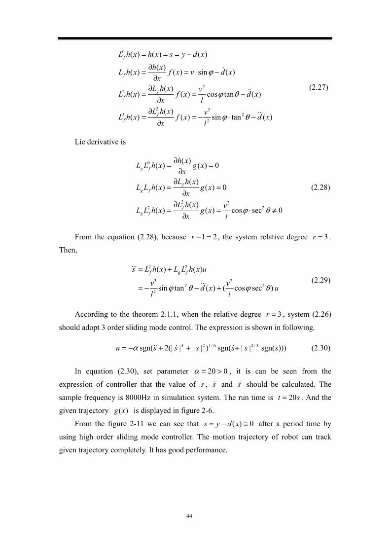
44
)(tansin)()(
)(
)(tancos)()(
)(
)(sin)()()(
)()()(
22
323
22
0
xdlvxf
xxhL
xhL
xdl
vxfx
xhLxhL
xdvxfxxhxhL
xdysxhxhL
ff
ff
f
f
−⋅−=∂
∂=
−=∂
∂=
−⋅=∂∂=
−===
θϕ
θϕ
ϕ
(2.27)
Lie derivative is
0seccos)()(
)(
0)()(
)(
0)()()(
222
2
0
≠⋅=∂
∂=
=∂
∂=
=∂∂=
θϕl
vxgx
xhLxhLL
xgx
xhLxhLL
xgxxhxhLL
ffg
ffg
fg
(2.28)
From the equation (2.28), because 21=−r , the system relative degree 3=r .
Then,
u
lvxd
lv
uxhLLxhLs fgf
)sec cos()(tansin
)()(
22
22
3
22
θϕθϕ +−−=
+= (2.29)
According to the theorem 2.1.1, when the relative degree 3=r , system (2.26)
should adopt 3 order sliding mode control. The expression is shown in following.
)))sgn(||sgn()|||(|2sgn( 3/26/123 ssssssu +++−= α (2.30)
In equation (2.30), set parameter 020 >=α , it is can be seen from the
expression of controller that the value of s , s and s should be calculated. The
sample frequency is 8000Hz in simulation system. The run time is st 20= . And the
given trajectory )(xg is displayed in figure 2-6.
From the figure 2-11 we can see that 0)( ≡−= xdys after a period time by
using high order sliding mode controller. The motion trajectory of robot can track
given trajectory completely. It has good performance.
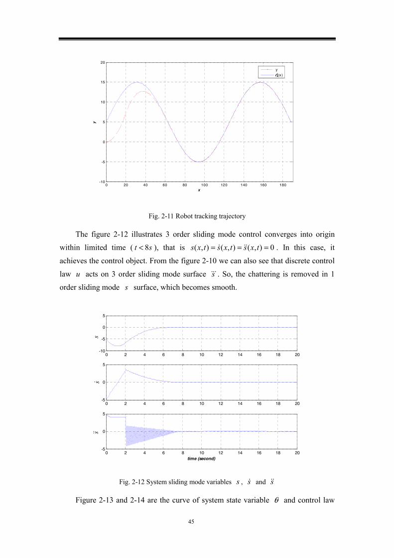
45
0 20 40 60 80 100 120 140 160 180-10
-5
0
5
10
15
20
x
y
y
g(x )
Fig. 2-11 Robot tracking trajectory
The figure 2-12 illustrates 3 order sliding mode control converges into origin
within limited time ( st 8< ), that is 0),(),(),( === txstxstxs . In this case, it
achieves the control object. From the figure 2-10 we can also see that discrete control
law u acts on 3 order sliding mode surface s . So, the chattering is removed in 1
order sliding mode s surface, which becomes smooth.
0 2 4 6 8 10 12 14 16 18 20-10
-5
0
5
s
0 2 4 6 8 10 12 14 16 18 20-5
0
5
s'
0 2 4 6 8 10 12 14 16 18 20-5
0
5
time (second)
s''
ss
s
Fig. 2-12 System sliding mode variables s , s and s
Figure 2-13 and 2-14 are the curve of system state variable θ and control law
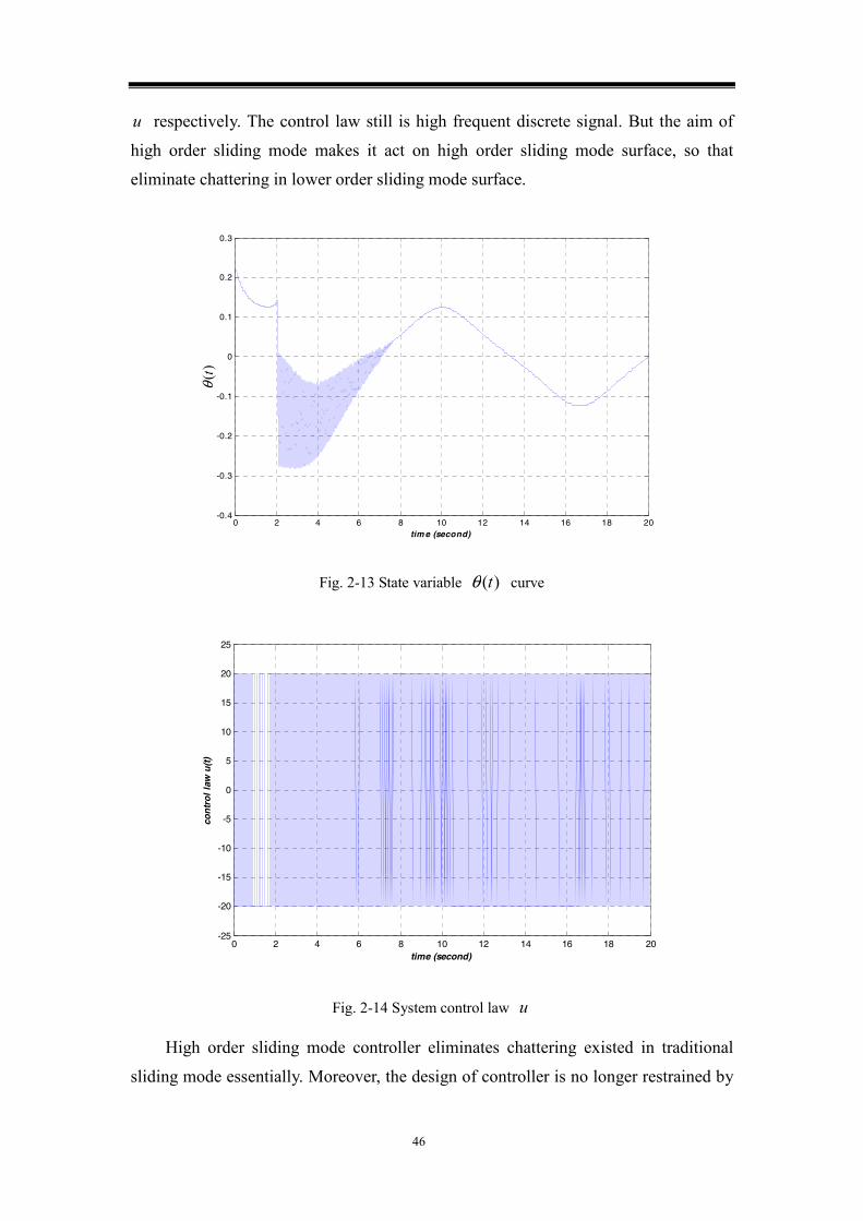
46
u respectively. The control law still is high frequent discrete signal. But the aim of
high order sliding mode makes it act on high order sliding mode surface, so that
eliminate chattering in lower order sliding mode surface.
0 2 4 6 8 10 12 14 16 18 20-0.4
-0.3
-0.2
-0.1
0
0.1
0.2
0.3
tim e (second)
θ (t
) )(tθ
Fig. 2-13 State variable )(tθ curve
0 2 4 6 8 10 12 14 16 18 20-25
-20
-15
-10
-5
0
5
10
15
20
25
time (second)
con
tro
l la
w u
(t)
Fig. 2-14 System control law u
High order sliding mode controller eliminates chattering existed in traditional
sliding mode essentially. Moreover, the design of controller is no longer restrained by

47
relative degree. It greatly enhances the applicability of the sliding mode control. In the
design of high order sliding mode controller, we only need to know sliding mode
variable and its corresponding derivatives. This controller has simple structure and is
easy to implement.
2.5 Quasi-continuous high order sliding mode control
In the design of high order sliding mode, the controller adopts high frequent sign
function. Because the relative degree ( 1=r ) of state variable θ to the control input
u is lowest, in the figure 2-8, the chattering phenomenon is the most serious as well.
In order to weaken or remove the effectiveness of chattering, according to the
homogeneous principle of high order sliding mode (Levant,2005), the control law is
),,(),,( )1(1)1( −−− = rrrr sssUsssU κκκ (2.31)
Where, 0>κ , it is arbitrary positive constant. When the system (2.18) satisfies
condition (2.21), then
uKKCCs Mmr ],[],[)( +−∈ (2.32)
Closed set differential equation (2.32) satisfies Filippov criterion (Filippov,1988).
That is the vector field in right half plane is extended to a special way to meet the
identified convex function and semi-continuous condition. Therefore, within the
limited time, the system (2.32) is stable at the origin. It is equivalent that the original
system (2.18) satisfies the conditions in (2.21) to converge into the origin.
0),(),(),( )1( ==== − txstxstxs r
Sufficiently large choice of parameters 121 ,, −rβββ , 0>α , according to the
homogeneous principle of high order sliding mode , a quasi-continuous sliding mode
controller can be designed, which is continuous except the points of
0)1( ==== −rsss . The detail expression is following.
),,,( )1(,1
−−Ψ−= r
rr sssu α (2.33)
Visually observe quasi-continuous sliding mode control (2.33), comparing with
high order sliding mode controller (2.22), the sign function is cancelled. The discrete
control law is transformed to continuous control law. Where,

48
1,1,0 ||
)sgn(||
,,,
)1/()(,1
)(,
,1)1/()(
,1)(
,
,0,0,0
,0
,0
−==Ψ+=
Ψ+=
==Ψ==
+−−−
−+−−
−
riNNsN
Ns
sNsN
s
ririri
irirrii
rri
riirir
riir
ri
rrr
r
r
ϕβ
βϕ
ϕ
ϕ
(2.34)
The controller (2.33) doesn’t erase sign function as well, so it is called
quasi-continuous high order sliding mode controller. In order to facilitate the use, let
11 =β , 22 =β , 33 =β , …, the expressions of 4≤r order is shown following
(Levant,2005).
2/13/24/3
2/13/24/34/33/14/3
2/13/2
3/22/13/2
2/1
2/1
])||5.0|(||[|3||])||5.0|(||))][|sgn(||5.0()||5.0|(|[3 .4
)|||(|2||)]sgn(||[)|||(|2 .3
||||)sgn(|| .2
)sgn( .1
ssssssssssssssu
sssssssssu
sssssu
su
+++++++++−=
+++++−=
++−=
−=
−−
−
α
α
α
α
If re-design the dynamic robot track trajectory system (2.12) adopting
quasi-continuous sliding mode controller, suppose other conditions unchanged, the
new controller can be written as
2/13/2
3/22/13/2
)|||(|2||)]sgn(||[)|||(|2
sssssssssu
+++++−=
−
α (2.35)
The figure 2-15 is tracking curve of robot motion trajectory. From this figure,
adopting quasi-continuous sliding mode control, the system output converges into
origin within limited time as well. In this case, it achieves higher precision tracking
control. In addition, the comparison of Figure 2-12 and 2-16, it is not difficult to find
the use of quasi-continuous high order sliding mode makes the first, second order
derivative of sliding mode variable more smooth than the previous high order sliding
mode control.

49
0 20 40 60 80 100 120 140 160 180-10
-5
0
5
10
15
20
x
y
yg(x)
Fig. 2-15 Robot tracking trajectory
0 2 4 6 8 10 12 14 16 18 20-10
-5
0
5
s
0 2 4 6 8 10 12 14 16 18 20-10
-5
0
5
s'
0 2 4 6 8 10 12 14 16 18 20-5
0
5
10
time (second)
s''
ss
s
Fig. 2-16 Sliding mode variables s , s and s
In high order sliding mode, because relative degree of state variable θ to
control input u equals to 1, θ is effected by discrete control law u greatly. From
the figure 2-13 we can see that the chattering is eliminated obviously. Through the
improvement of control law, without affecting the accuracy of the premise, as far as
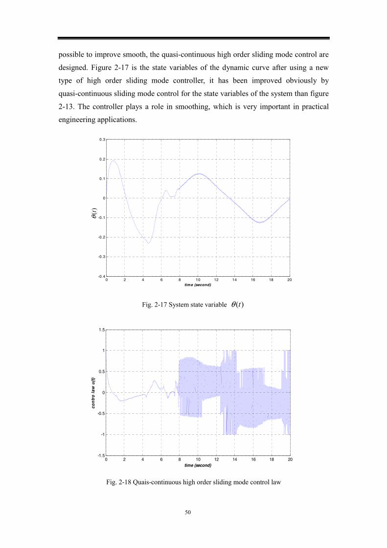
50
possible to improve smooth, the quasi-continuous high order sliding mode control are
designed. Figure 2-17 is the state variables of the dynamic curve after using a new
type of high order sliding mode controller, it has been improved obviously by
quasi-continuous sliding mode control for the state variables of the system than figure
2-13. The controller plays a role in smoothing, which is very important in practical
engineering applications.
0 2 4 6 8 10 12 14 16 18 20-0.4
-0.3
-0.2
-0.1
0
0.1
0.2
0.3
time (second)
θ(t) )
(tθ
Fig. 2-17 System state variable )(tθ
0 2 4 6 8 10 12 14 16 18 20-1.5
-1
-0.5
0
0.5
1
1.5
time (second)
con
tro
law
u(t)
Fig. 2-18 Quais-continuous high order sliding mode control law

51
Figure 2-18 is a quasi-continuous high-order sliding mode control law curve.
Comparing with the higher order sliding mode controller, especially before entering
the sliding mode, the switching frequency is reduced.
2.6 Summary
This chapter from a simple beginning of the second-order sliding mode control,
the step by step analyses the causes how the second order sliding mode control
eliminates chattering essentially. The second order sliding mode control algorithm is
still strict requirements of the system relative degree, so design of arbitrary order
controller is necessary. In view of this consideration, this chapter gives a high order
(arbitrary order) sliding mode control algorithm, combined with a simulation example
for the simulation studies. The simulation results show that the high order sliding
mode control achieves higher precious trajectory tracked. At the same time, the
quasi-continuous high-order sliding mode control algorithm is given to smooth the
system state variable.

52
Chapter 3 Robust exact high order sliding mode differentiator
To get the differentiation of a given signal is always to be studied. In automatic
control systems, we often need derivative a variable or function. So there are a lot of
numerical algorithms for this issue. The same situation also appears in the design of
high order sliding mode controller (2.24) that needs to calculate the derivative values
of sliding mode variable. In order to be able to accurately calculate, at the same time
simplifying the algorithm, this chapter directly uses own advantages of high order
sliding mode control due to high accuracy and robustness. We can design a high order
sliding mode differentiator used to calculate the numerical derivative of the variables
(Levant,2003).
Presentation in the previous chapter has been explained in detail the principles of
high order sliding mode control and sliding mode controller design method. This
chapter focuses on how to take use of high order sliding mode technique to solve the
differentiation of a given signal or variable function. And their simulation results are
verified.
This chapter is structured as follows: 3.1, derive a robust sliding mode
differentiator; 3.2, verify its feasibility with the numerical simulation; 3.3, give the
high order sliding mode differentiator used to solve arbitrary order derivative; 3.4 take
a simulation example of arbitrary order sliding mode differentiator applications; 3.5,
summary of this chapter.
3.1 Robust sliding mode differentiator
Suppose given signal is )(tf , now set a dynamic system as
ux = (3.1)
The control object is to make the variable x follow given signal )(tf , that is
)(tfx = (3.2)
Therefore, sliding mode surface is selected as
)(tfxs −= (3.3)
At this moment, according to the principle of sliding mode control, a proper
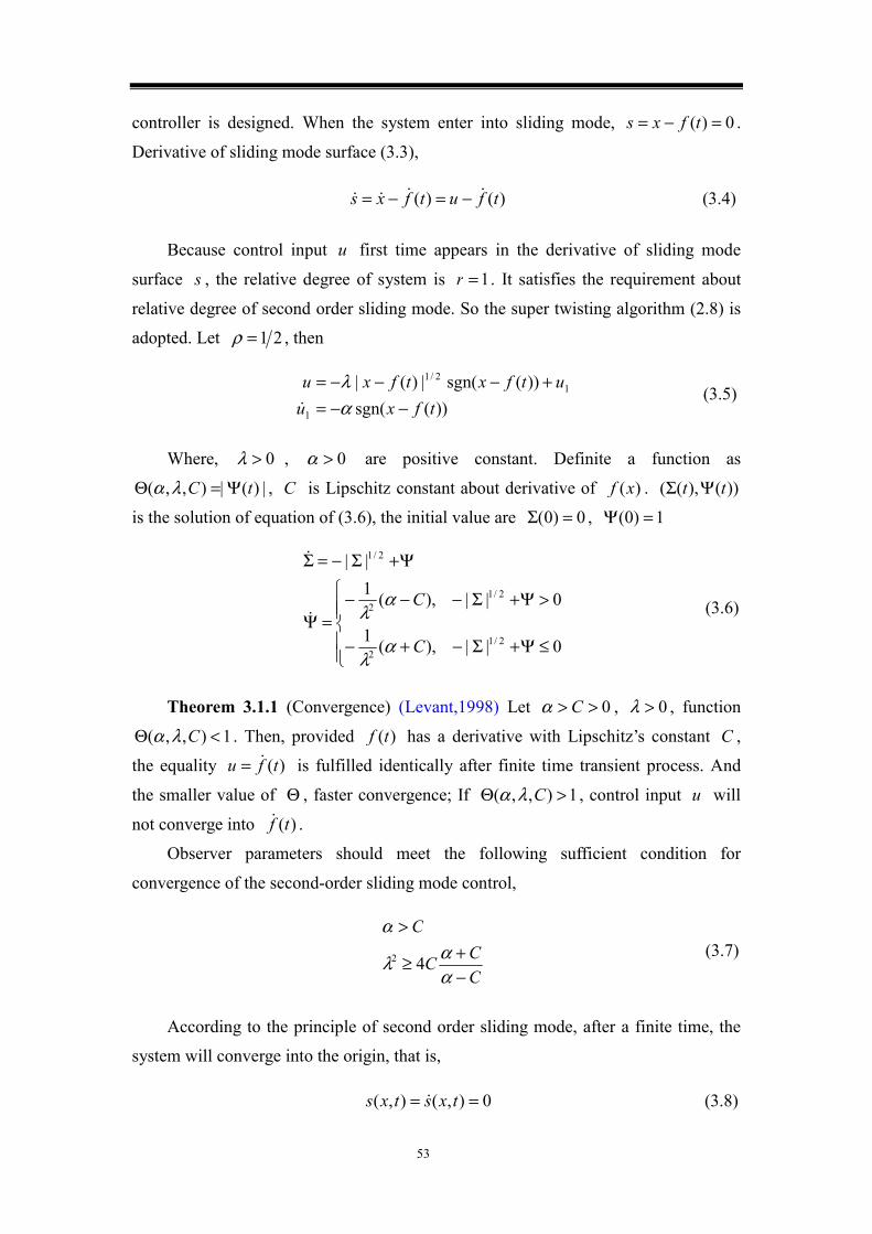
53
controller is designed. When the system enter into sliding mode, 0)( =−= tfxs .
Derivative of sliding mode surface (3.3),
)()( tfutfxs −=−= (3.4)
Because control input u first time appears in the derivative of sliding mode
surface s , the relative degree of system is 1=r . It satisfies the requirement about
relative degree of second order sliding mode. So the super twisting algorithm (2.8) is
adopted. Let 21=ρ , then
))(sgn(
))(sgn(|)(|
1
12/1
tfxuutfxtfxu
−−=+−−−=
αλ
(3.5)
Where, 0>λ , 0>α are positive constant. Definite a function as
|)(|),,( tC Ψ=Θ λα , C is Lipschitz constant about derivative of )(xf . ))(),(( tt ΨΣ
is the solution of equation of (3.6), the initial value are 0)0( =Σ , 1)0( =Ψ
⎪⎪⎩
⎪⎪⎨
⎧
≤Ψ+Σ−+−
>Ψ+Σ−−−=Ψ
Ψ+Σ−=Σ
0|| ),(1
0|| ),(1||
2/12
2/12
2/1
C
C
αλ
αλ (3.6)
Theorem 3.1.1 (Convergence) (Levant,1998) Let 0>> Cα , 0>λ , function
1),,( <Θ Cλα . Then, provided )(tf has a derivative with Lipschitz’s constant C ,
the equality )(tfu = is fulfilled identically after finite time transient process. And
the smaller value of Θ , faster convergence; If 1),,( >Θ Cλα , control input u will
not converge into )(tf .
Observer parameters should meet the following sufficient condition for
convergence of the second-order sliding mode control,
CCC
C
−+≥
>
ααλ
α
42 (3.7)
According to the principle of second order sliding mode, after a finite time, the
system will converge into the origin, that is,
0),(),( == txstxs (3.8)
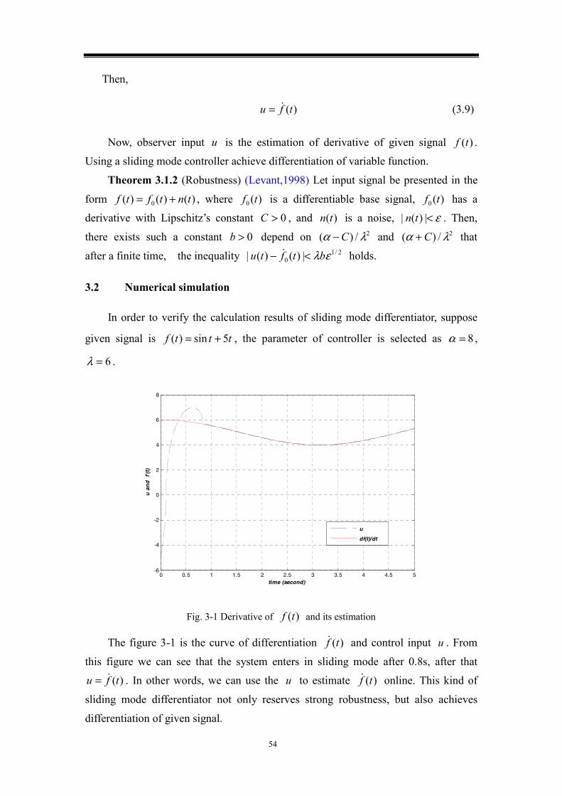
54
Then,
)(tfu = (3.9)
Now, observer input u is the estimation of derivative of given signal )(tf .
Using a sliding mode controller achieve differentiation of variable function.
Theorem 3.1.2 (Robustness) (Levant,1998) Let input signal be presented in the
form )()()( 0 tntftf += , where )(0 tf is a differentiable base signal, )(0 tf has a
derivative with Lipschitz’s constant 0>C , and )(tn is a noise, ε<|)(| tn . Then,
there exists such a constant 0>b depend on 2/)( λα C− and 2/)( λα C+ that
after a finite time, the inequality 2/10 |)()(| ελbtftu <− holds.
3.2 Numerical simulation
In order to verify the calculation results of sliding mode differentiator, suppose
given signal is tttf 5sin)( += , the parameter of controller is selected as 8=α ,
6=λ .
0 0.5 1 1.5 2 2.5 3 3.5 4 4.5 5-6
-4
-2
0
2
4
6
8
time (second)
u a
nd
f'(
t)
u
df(t)/dt
Fig. 3-1 Derivative of )(tf and its estimation
The figure 3-1 is the curve of differentiation )(tf and control input u . From
this figure we can see that the system enters in sliding mode after 0.8s, after that
)(tfu = . In other words, we can use the u to estimate )(tf online. This kind of
sliding mode differentiator not only reserves strong robustness, but also achieves
differentiation of given signal.

55
0 0.5 1 1.5 2 2.5 3 3.5 4 4.5 5-6
-4
-2
0
2
4
6
8
time (second)
u a
nd
f'(
t)
u without noise
df(t)/dt
u with noise
Fig. 3-2 Signal u is estimation of )(tf under disturbance
The figure 3-2 illustrates sliding mode differentiator has strong robustness for the
estimation of )(tf in spit of external disturbance. After a short time adjusting, the
system still can converge into origin.
0 1 2 3 4 5 6 7 8 9 10-0.8
-0.6
-0.4
-0.2
0
0.2
0.4
0.6
0.8
1
time (second)
dis
turb
ance
Fig. 3-3 Disturbance signal )2sin(2.0 ten t−=
The disturbance signal injected is )2sin()( 2.0 tetn t−= , which is shown in figure
3-3. The figure 3-4 is the error between differentiator estimation and actual derivative
of function )(tf . The error is less than 310− , that is 310|)(| −<− tfu .

56
1 1.5 2 2.5 3 3.5 4-0.01
-0.008
-0.006
-0.004
-0.002
0
0.002
0.004
0.006
0.008
0.01
time (second)
erro
r
Fig. 3-4 The error between u and )(tf despite disturbance
To sum up, sliding mode differentiator not only can achieve precious estimation
for derivative of given signal, but also has robust characteristics of its own. Therefore,
the differentiator has a broad application and practical value.
3.3 Arbitrary order sliding mode differentiator
Through the first order sliding mode differentiator description of the working
principle, it will naturally think, whether can design a sliding mode differentiator to
obtain the arbitrary order derivative of given signal. Well, the design of high order
sliding mode controller (2.24) needs to know all sliding mode variables and their
corresponding differentiation. If we can design an arbitrary order sliding mode
differentiator, which can be used to estimate the derivative value of sliding mode
variables, so as to achieve a simplified numerical differential purposes.
The same with first order sliding mode differentiator, suppose given signal is
)(tf , ),0[ ∞∈t . It has been known that the n order derivative of )(tf has
Lipschitz constant, recorded as 0>L . Now, the object of sliding mode differentiator
is estimating the value of )(,),(),( )( tftftf n in real time.
Arbitrary order sliding mode differentiator has the following recursive form,

57
)sgn(,)sgn(||
,)sgn(||
,))(sgn(|)(|
1
212/1
2111
11
201/)1(
0111
11
10)1/(
000
00
−
−−−−−−
−−
−
+
−−=+−−−=
=
+−−−=
=+−−−=
=
nnnn
nnnnnnn
nn
nn
nn
vzzzvzvzv
vz
zvzvzv
vzztfztfzv
vz
λλ
λ
λ
(3.10)
It can be verified, When 1=n , it is first order differentiator. Suppose )(0 tf is
basic value of given signal )(tf , )(tδ is uncertain part, but bounded, satisfying
εδ <|)(| t , then )()()( 0 ttftf δ+= .
Theorem 3.3.1 (Levant,2003) If properly choose parameter )0( nii ≤≤λ , the
following equalities are true in the absence of input noise after a finite time of a
transient process.
nitfvz
tfzi
ii ,,1 ),(
)()(
0
00
===
= (3.11)
The theorem 3.3.1 illustrates that arbitrary order sliding mode differentiator can
use differentiation )0( nizi ≤≤ to estimate any order derivative of input function
)(tf online within limited time.
Theorem 3.3.2 (Levant,2003) Let the input noise satisfy the inequality
εδ ≤−= |)()(|)( 0 tftft . Then the following inequality are established in finite time
for some positive constants iμ , iτ depending exclusively on the parameters of the
differentiator
1,,0 |)(|
,,0 |)(|)1/()()1(
0
)1/()1()(0
−=≤−
=≤−+−+
++−
nitfv
nitfznin
ii
i
nini
ii
ετεμ
(3.12)
By Theorem 3.3.2, we can see that the arbitrary order sliding mode differentiator
has robustness.
The arbitrary order sliding mode differentiator can accurately estimate any order
derivative of a given input. If this differentiator can be used in high order sliding
mode controller (2.24), any order derivative of sliding mode variable s can be
accurately estimated avoiding the complicated calculation, which greatly simplifies

58
the controller design. Adopting the differentiator, consider )(ts in high order sliding
mode controller as given input for differentiator. Then the output of differentiator
)0( nizi ≤≤ can substitute any order derivative of )(ts , that is
nisz
szi
i ,1 )(
0
==
= (3.13)
The sliding mode controller (2.22) can be rewritten by
)),,,(sgn( )1(10,1 −−−= rrr zzzu ψα (3.14)
The expression from this controller can also be clearly seen, with high order
sliding mode differentiator, the differentiation of arbitrary order sliding mode variable
will not be difficult to solve, which makes the high order sliding mode controller
design has been simplified greatly.
3.4 Simulation example
In order to facilitate description and comparison, the system still uses the robot
model (2.21). Owing to system relative degree with 3=r , the controller adopted
should be
)))sgn(||sgn()|||(|2sgn( 3/26/123 ssssssu +++−= α (3.15)
If without sliding mode differentiator, the controller should calculate the value of
s , s and s . Taking use of differentiator, variable s is considered as given input of
the differentiator. Then, the output of differentiator z can be used to estimate
corresponding order derivative of s . The following design of differentiator is given
||440
)sgn(||30 ,
)sgn(||7.14 ,
122
2012/1
01111
103/2
0000
ννννν
νν
−−=+−−−==
+−−−==
zzzzzz
zszszz
(3.16)
Now, according theorem 3.3.1, controller (3.15) can be rewritten by
)))sgn(||sgn()|||(|2sgn( 03/2
016/12
03
12 zzzzzzu +++−= α (3.17)
Where, control parameter 01>=α ; sliding mode differentiator parameters
7.140 =λ , 301 =λ and 4402 =λ .

59
0 20 40 60 80 100 120 140 160 180-10
-5
0
5
10
15
20
x
y
yg(x)
Fig. 3-5 Robot tracking trajectory curve
The figure 3-5 is the robot tracking trajectory curve using arbitrary order sliding
mode differentiator. Compared with figure 2-6, the system has the same tracking
effectiveness, which illustrates sliding mode differentiator with a good performance.
Its main advantage is any order differentiations only based on sliding mode variable
can be obtained. Thus, it eliminates the need of the arbitrary order derivative
calculations in high order sliding mode controller.
0 2 4 6 8 10 12 14 16 18 20-10
-5
0
5
z 0
0 2 4 6 8 10 12 14 16 18 20-10
-5
0
5
z 1
0 2 4 6 8 10 12 14 16 18 20-5
0
5
time (second)
z 20z
1z2z
Fig. 3-6 differentiator output 0z , 1z and 2z
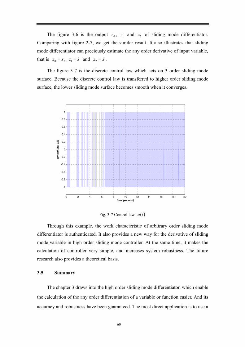
60
The figure 3-6 is the output 0z , 1z and 2z of sliding mode differentiator.
Comparing with figure 2-7, we get the similar result. It also illustrates that sliding
mode differentiator can preciously estimate the any order derivative of input variable,
that is sz =0 , sz =1 and sz =2 .
The figure 3-7 is the discrete control law which acts on 3 order sliding mode
surface. Because the discrete control law is transferred to higher order sliding mode
surface, the lower sliding mode surface becomes smooth when it converges.
0 2 4 6 8 10 12 14 16 18 20
-1
-0.8
-0.6
-0.4
-0.2
0
0.2
0.4
0.6
0.8
1
time (second)
con
tro
l la
w u
(t)
Fig. 3-7 Control law )(tu
Through this example, the work characteristic of arbitrary order sliding mode
differentiator is authenticated. It also provides a new way for the derivative of sliding
mode variable in high order sliding mode controller. At the same time, it makes the
calculation of controller very simple, and increases system robustness. The future
research also provides a theoretical basis.
3.5 Summary
The chapter 3 draws into the high order sliding mode differentiator, which enable
the calculation of the any order differentiation of a variable or function easier. And its
accuracy and robustness have been guaranteed. The most direct application is to use a

61
high order sliding mode differentiator to solve a sliding variable and its any order
derivative value. In this way, the calculation becomes simply, and the high order
sliding mode controller design is facilitating. At the same time, taking advantage of
this differentiator can be implemented with observation online.
62
Chapter 4 Application — Nonlinear permanent magnetic
synchronous motor high order sliding mode control
Permanent magnet synchronous motors (PMSM) are receiving increased
attention for electric drive applications due to their high power density, large torque to
inertia ratio and high efficiency over other kinds of motors (Glumineau,1993;
Ziribi,2001; Caravani,1998).
But the dynamic model of a PMSM is highly nonlinear because of the coupling
between the motor speed and the electrical quantities, such as the d, q axis currents. In
last years, many different control algorithms have been used to improve the
performance of the magnet motor. For example, as the dynamic model of the machine
is nonlinear, a natural approach is the exact feedback linearization control method, by
which the original nonlinear model can be transformed into a linear model through
proper coordinate transformation. However, in general, the dynamics of the
synchronous motors may not be fully known, since some of parameters appearing in
the equations will vary. For instance, the resistance and inductance will be changed
when the temperature alters. As a consequence, nonlinearities can only be partially
cancelled by the feedback linearization technique, and parameters uncertainties act on
the equations of the motion. Then an important aim of the control design is to develop
a robust controller which ensures good dynamic performances in spite of parameters
uncertainties and perturbation.
The sliding mode control is known to be a robust approach to solve the control
problems of nonlinear systems. Robustness properties against various kinds of
uncertainties such as parameter perturbations and external disturbances can be
guaranteed. However, this control strategy has a main drawback: the well known
chattering phenomenon. In order to reduce the chattering, the sign function can be
replaced by a smooth approximation. However, this technique induces deterioration in
accuracy and robustness. In last decade, another approach called higher order sliding
mode (HOSM) has been proposed and developed. It is the generalization of classical
sliding mode control and can be applied to control systems with arbitrary relative
degree r respecting to the considered output. In HOSM control, the main objective is
to obtain a finite time convergence in the non empty manifold
}0|{ )1( ==⋅⋅⋅===∈= −rssssXxS by acting discontinuously on r order
63
derivatives of the sliding variable s. Advantageous properties of HOSM are: the
chattering effect is eliminated, higher order precision is provided whereas all the
qualities of standard sliding mode are kept, and control law is not limited by relative
degree of the output.
This chapter is structured as follows: 4.1, derive mathematical model of PMSM;
4.2, propose the robust control for permanent magnet synchronous motor using high
order sliding mode control and nonlinear decoupling technique; 4.3, propose an
estimation method by using higher order sliding mode controller with differentiator to
achieve a synchronous motor state variable estimation online; 4.4, according to the
principle of high order sliding mode control and differentiator, the external
disturbance torque of the motor is estimated online successfully; 4.5, Summary of this
chapter.
4.1 Mathematical model of PMSM
The common analysis of permanent magnet synchronous motor is d-q axis
mathematical model. It can be used to analyze not only the permanent magnet
synchronous motor steady state operating characteristics, but also can be used to
analyze the transient performance motor (Tang Ren-Yuan, 2002). In order to establish
sinusoidal PMSM d-q axis mathematical model, firstly assume:
I. motor core saturation neglected;
II. Excluding the eddy current and magnetic hysteresis loss of motor;
III. The motor current is symmetrical three phase sine wave current.
Thereby, the following voltage, flux linkage, electromagnetic torque and
mechanical motion equations can be obtained, where all the values in equations are
transient.
The voltage equation:
qdq
q
dqd
d
Ridt
du
Ridt
du
++=
+−=
ωψψ
ωψψ
(4.1)
The flux linkage equation:
qqq
fddd
iLiL
=
+=
ψψψ
(4.2)

64
The electromagnetic torque equation:
])[(
)(
qfqdqd
dqqdem
iiiLLPiiPT
ψψψ
+−=
−= (4.3)
The motor motion equation:
Ω−−=Ω BTTdtdJ lem (4.4)
Where: du 、 qu —— d-q axis stator voltage;
di 、 qi —— d-q axis stator current;
dL 、 qL —— d-q axis stator inductance, when qd LL = , motor is
non-salient pole; when qd LL < , motor is salient pole;
dψ 、 qψ —— d-q axis stator flux linkage;
fψ —— magnetic potential generated by permanent magnet rotor;
ω—— motor’s electrical angular velocity;
R —— stator phase resistance;
P —— number of motor pole pairs;
emT —— electromagnetic torque;
lT —— load torque;
Ω—— motor’s mechanical angular velocity, with ωP=Ω ;
J —— total inertia of rotor and load;
B —— viscous friction coefficient.
Set of equations (4.1), (4.2), (4.3) and (4.4), we can get the state equation
expression of PMSM as following.
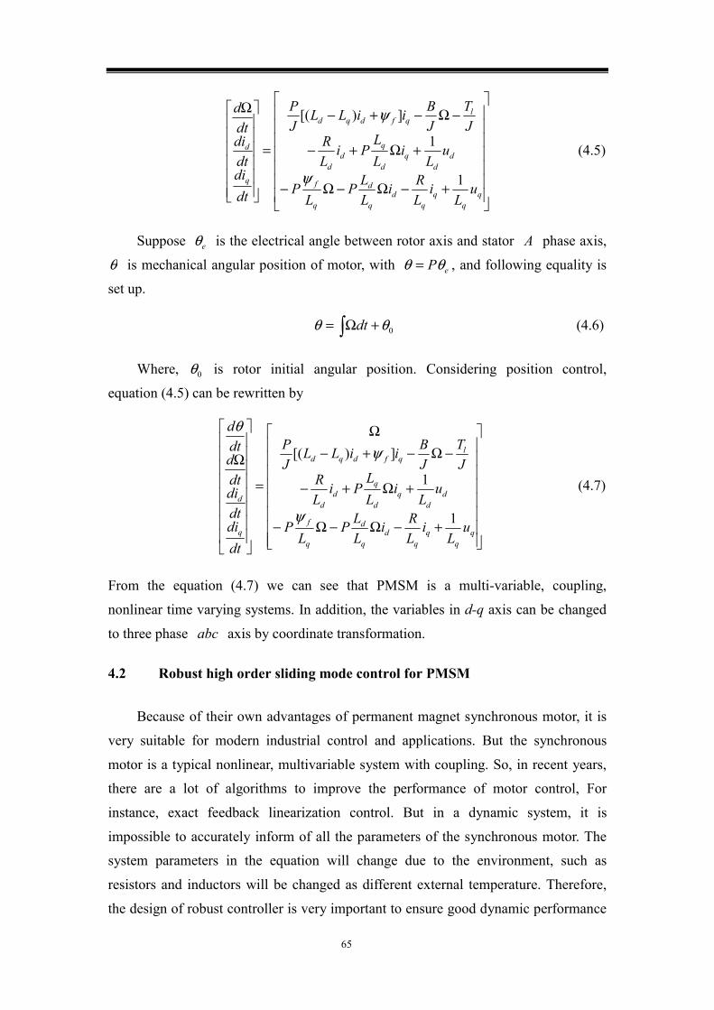
65
⎥⎥⎥⎥⎥⎥⎥
⎦
⎤
⎢⎢⎢⎢⎢⎢⎢
⎣
⎡
+−Ω−Ω−
+Ω+−
−Ω−+−
=
⎥⎥⎥⎥⎥⎥
⎦
⎤
⎢⎢⎢⎢⎢⎢
⎣
⎡ Ω
dq
d
q
f
dd
qd
qd
d
lqfdqd
q
d
uL
iLRi
LLP
LP
uL
iLL
PiLR
JT
JBiiLL
JP
dtdidtdidtd
1
1
])[(
ψ
ψ
(4.5)
Suppose eθ is the electrical angle between rotor axis and stator A phase axis,
θ is mechanical angular position of motor, with ePθθ = , and following equality is
set up.
∫ +Ω= 0θθ dt (4.6)
Where, 0θ is rotor initial angular position. Considering position control,
equation (4.5) can be rewritten by
⎥⎥⎥⎥⎥⎥⎥⎥
⎦
⎤
⎢⎢⎢⎢⎢⎢⎢⎢
⎣
⎡
+−Ω−Ω−
+Ω+−
−Ω−+−Ω
=
⎥⎥⎥⎥⎥⎥⎥⎥
⎦
⎤
⎢⎢⎢⎢⎢⎢⎢⎢
⎣
⎡
Ω
dq
d
q
f
dd
qd
qd
d
lqfdqd
q
d
uL
iLRi
LLP
LP
uL
iLL
PiLR
JT
JBiiLL
JP
dtdidtdidtddtd
1
1
])[(
ψ
ψ
θ
(4.7)
From the equation (4.7) we can see that PMSM is a multi-variable, coupling,
nonlinear time varying systems. In addition, the variables in d-q axis can be changed
to three phase abc axis by coordinate transformation.
4.2 Robust high order sliding mode control for PMSM
Because of their own advantages of permanent magnet synchronous motor, it is
very suitable for modern industrial control and applications. But the synchronous
motor is a typical nonlinear, multivariable system with coupling. So, in recent years,
there are a lot of algorithms to improve the performance of motor control, For
instance, exact feedback linearization control. But in a dynamic system, it is
impossible to accurately inform of all the parameters of the synchronous motor. The
system parameters in the equation will change due to the environment, such as
resistors and inductors will be changed as different external temperature. Therefore,
the design of robust controller is very important to ensure good dynamic performance
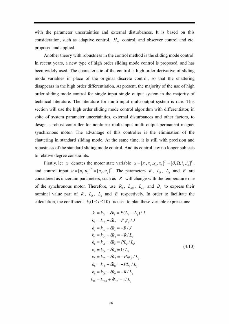
66
with the parameter uncertainties and external disturbances. It is based on this
consideration, such as adaptive control, ∞H control, and observer control and etc.
proposed and applied.
Another theory with robustness in the control method is the sliding mode control.
In recent years, a new type of high order sliding mode control is proposed, and has
been widely used. The characteristic of the control is high order derivative of sliding
mode variables in place of the original discrete control, so that the chattering
disappears in the high order differentiation. At present, the majority of the use of high
order sliding mode control for single input single output system in the majority of
technical literature. The literature for multi-input multi-output system is rare. This
section will use the high order sliding mode control algorithm with differentiator, in
spite of system parameter uncertainties, external disturbances and other factors, to
design a robust controller for nonlinear multi-input multi-output permanent magnet
synchronous motor. The advantage of this controller is the elimination of the
chattering in standard sliding mode. At the same time, it is still with precision and
robustness of the standard sliding mode control. And its control law no longer subjects
to relative degree constraints.
Firstly, let x denotes the motor state variable Tqd
T iixxxxx ],,,[],,,[ 4321 Ω== θ ,
and control input Tqd
T uuuuu ],[],[ 21 == . The parameters R , dL , qL and B are
considered as uncertain parameters, such as R will change with the temperature rise
of the synchronous motor. Therefore, use 0R , 0dL , 0qL and 0B to express their
nominal value part of R , dL , qL and B respectively. In order to facilitate the
calculation, the coefficient )101( ≤≤ iki is used to plan these variable expressions:
q
q
qd
qf
d
dq
d
f
qd
LkkkLRkkk
LPLkkkLPkkk
Lkkk
LPLkkkLRkkkJBkkk
JPkkkJLLPkkk
/1/
//
/1
///
//)(
1001010
9099
8088
7077
6066
5055
4044
3033
2022
1011
=+=
−=+=
−=+=
−=+==+=
=+=−=+=−=+=
=+=
−=+=
δδδ
ψδδδδδ
ψδδ
(4.10)

67
Where, )101(0 ≤≤ ik i is the nominal value of the concerned parameter, ikδ is
the uncertainty on the concerned parameter such that |||| 00 iii kkk ≤≤ δδ , with ik0δ a
known positive bound. The state variable 4Rx∈ , such that )42(|| ≤≤≤ ixx iMAXi ,
MAXx2 is the maximum values of the angular velocity, MAXx3 and MAXx4 are the
maximum values of the current di and qi respectively. And control input 2Ru∈
such that )21(,|| ≤≤≤ iuu iMAXi . Where, MAXu1 and MAXu2 are the maximum values
of the voltage input dv and qv respectively.
Then the state space model of the synchronous motor can be changed as
following nonlinear system.
⎥⎦
⎤⎢⎣
⎡
⎥⎥⎥⎥
⎦
⎤
⎢⎢⎢⎢
⎣
⎡
+
⎥⎥⎥⎥
⎦
⎤
⎢⎢⎢⎢
⎣
⎡
+++
−++=
⎥⎥⎥⎥
⎦
⎤
⎢⎢⎢⎢
⎣
⎡
2
1
),(
10
6
),(
4932827
42534
234231
2
4
3
2
1
000000
/)(uu
kk
xkxxkxkxxkxk
JTxkxkxkx
xxxx
txgtxf
l (4.11)
The aim is to design an appropriate control which guarantees robust performance
in presence of parameters and load variations. The control objective is double aspect.
First, the rotor angular position θ=1x must track a reference trajectory angular
position refx1 . Second, the nonlinear electromagnetic torque must be linearized to
avoid reluctance effects and torque ripple. This objective is equivalent to constrain
dix =3 to track a constant direct current reference 03 =refx .
As we known that PMSM is a multi-input multi-output nonlinear dynamic
system. It is assumed that the position and current are available for measurement. A
first sliding variable s for the tracking of direct current 3x towards its equilibrium
point refx3 f is defined from the direct current error. So, the first sliding mode
variable is
refxxxhs 3311 )( −== (4.12)
Derivative of 1s , we can see that the relative degree of sliding mode variable 1s
equals 1, that is
ref
ref
xukxxkxkxxs
31642534
331
−++=
−= (4.13)
To track the angular position θ=1x , another sliding manifold is proposed so
that the error dynamics follows a desired third order dynamic. Denoting refx1 the
desired trajectory, following form can be obtained.
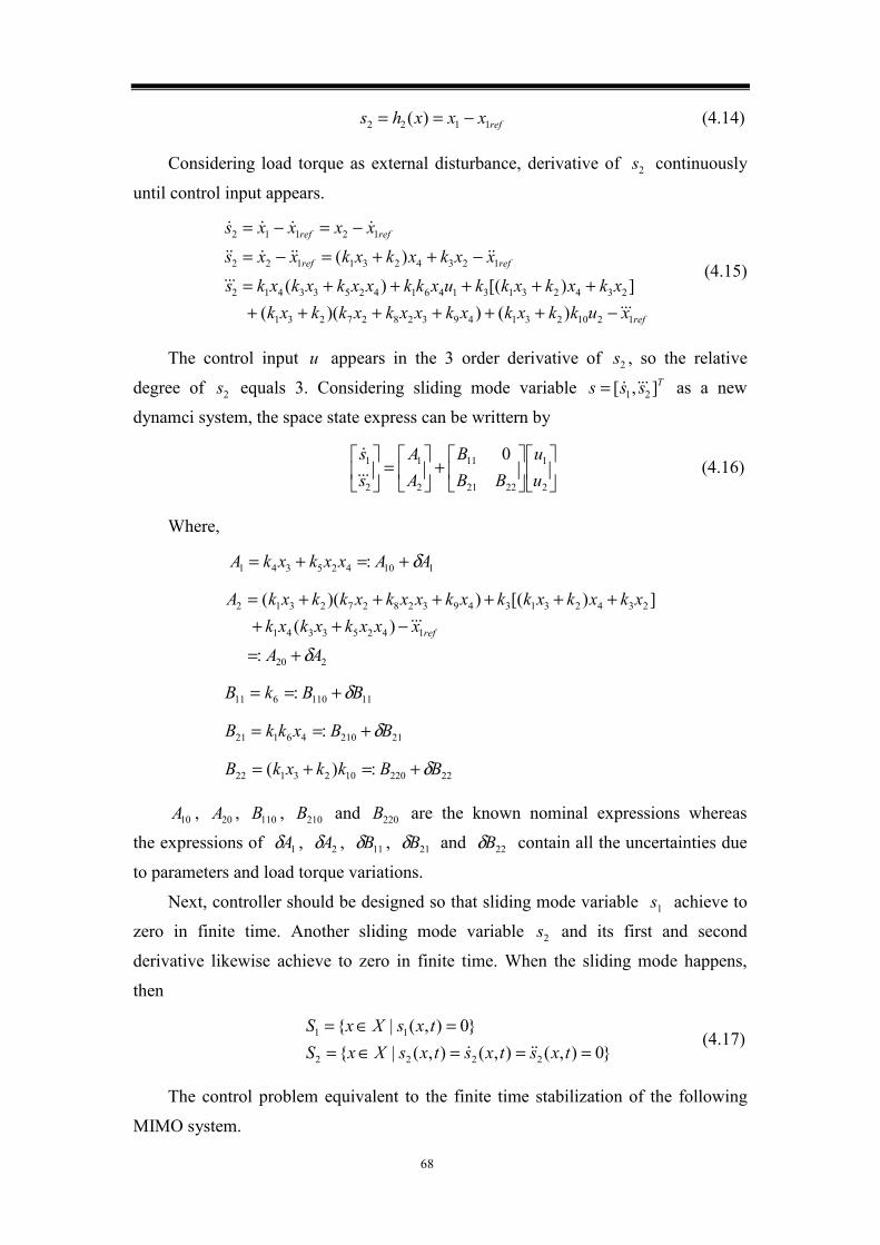
68
refxxxhs 1122 )( −== (4.14)
Considering load torque as external disturbance, derivative of 2s continuously
until control input appears.
ref
refref
refref
xukkxkxkxxkxkkxkxkxkxkkuxkkxxkxkxks
xxkxkxkxxs
xxxxs
12102314932827231
2342313146142533412
1234231122
12112
)())((])[()(
)(
−+++++++++++=
−++=−=
−=−=
(4.15)
The control input u appears in the 3 order derivative of 2s , so the relative
degree of 2s equals 3. Considering sliding mode variable Tsss ],[ 21= as a new
dynamci system, the space state express can be writtern by
⎥⎦
⎤⎢⎣
⎡⎥⎦
⎤⎢⎣
⎡+⎥
⎦
⎤⎢⎣
⎡=⎥
⎦
⎤⎢⎣
⎡
2
1
2221
11
2
1
2
1 0uu
BBB
AA
ss
(4.16)
Where,
110425341 : AAxxkxkA δ+=+=
220
14253341
234231349328272312
:
)(])[())((
AA
xxxkxkxkxkxkxkkxkxxkxkkxkA
ref
δ+=
−++++++++=
11110611 : BBkB δ+==
2121046121 : BBxkkB δ+==
222201023122 :)( BBkkxkB δ+=+=
10A , 20A , 110B , 210B and 220B are the known nominal expressions whereas
the expressions of 1Aδ , 2Aδ , 11Bδ , 21Bδ and 22Bδ contain all the uncertainties due
to parameters and load torque variations.
Next, controller should be designed so that sliding mode variable 1s achieve to
zero in finite time. Another sliding mode variable 2s and its first and second
derivative likewise achieve to zero in finite time. When the sliding mode happens,
then
}0),(),(),(|{
}0),(|{
2222
11
===∈==∈=
txstxstxsXxStxsXxS
(4.17)
The control problem equivalent to the finite time stabilization of the following
MIMO system.

69
⎥⎦
⎤⎢⎣
⎡+=⎥
⎦
⎤⎢⎣
⎡
2
1
2
1
uu
BAss
(4.18)
Where,
AAAA
AA
A δδδ
+=⎥⎦
⎤⎢⎣
⎡+⎥
⎦
⎤⎢⎣
⎡= 0
2
1
20
10 : (4.19)
BBBB
BBB
BB δ
δδδ
+=⎥⎦
⎤⎢⎣
⎡+⎥
⎦
⎤⎢⎣
⎡= 0
2221
11
220210
110 :00
(4.20)
From the equation (4.15), the outputs of this MIMO system are coupled since 2s
is affected by 1u and 2u . So a input-output feedback linearization technique can be
used
][ 01
0 wABu +−⋅= − (4.21)
Now, if considering influence of external disturbance and parameter
uncertainties , equation (4.18) can be rewritten by
)]()[(
)(
01
000
00
wABBBAA
uBBAABuAs
+−+++=
+++=+=
−δδδδ (4.22)
Evolute and ordinate, then
⎥⎦
⎤⎢⎣
⎡⎥⎦
⎤⎢⎣
⎡+⎥
⎦
⎤⎢⎣
⎡=⎥
⎦
⎤⎢⎣
⎡⇒
2
1
2221
11
2
1
2
1
ˆˆ0ˆ
ˆˆ
ww
BBB
AA
ss
(4.23)
Where,
10110
1111
ˆ ABBAA δδ −=
20220
2210
220110
21022
110
2122 ][ˆ A
BBA
BBBB
BBAA δδδδ −−−=
110
1111 1ˆ
BBB δ+=
220110
21022
110
2121
ˆBBBB
BBB δδ −=
220
2222 1ˆ
BBB δ+=
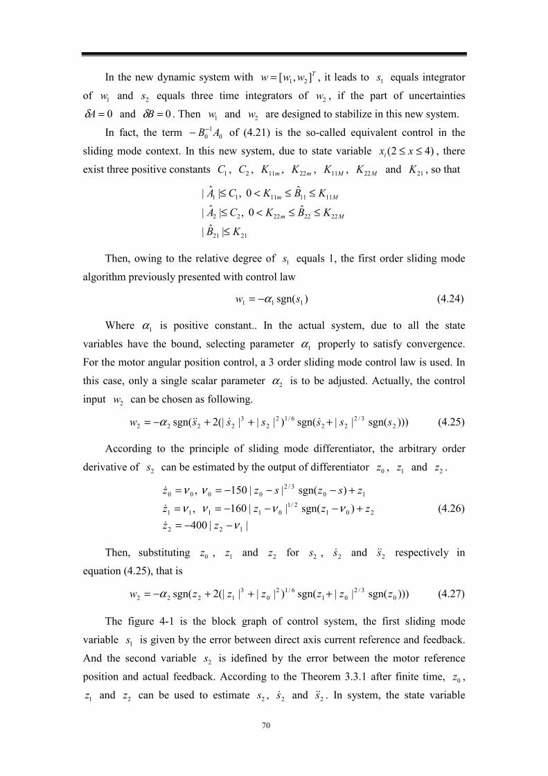
70
In the new dynamic system with Twww ],[ 21= , it leads to 1s equals integrator
of 1w and 2s equals three time integrators of 2w , if the part of uncertainties
0=Aδ and 0=Bδ . Then 1w and 2w are designed to stabilize in this new system.
In fact, the term 01
0 AB−− of (4.21) is the so-called equivalent control in the
sliding mode context. In this new system, due to state variable )42( ≤≤ xxi , there
exist three positive constants 1C , 2C , mK11 , mK22 , MK11 , MK22 and 21K , so that
2121
22222222
11111111
|ˆ|
ˆ0 ,|ˆ|
ˆ0 ,|ˆ|
KB
KBKCA
KBKCA
Mm
Mm
≤
≤≤<≤
≤≤<≤
Then, owing to the relative degree of 1s equals 1, the first order sliding mode
algorithm previously presented with control law
)sgn( 111 sw α−= (4.24)
Where 1α is positive constant.. In the actual system, due to all the state
variables have the bound, selecting parameter 1α properly to satisfy convergence.
For the motor angular position control, a 3 order sliding mode control law is used. In
this case, only a single scalar parameter 2α is to be adjusted. Actually, the control
input 2w can be chosen as following.
)))sgn(||sgn()|||(|2sgn( 23/2
226/12
23
2222 ssssssw +++−= α (4.25)
According to the principle of sliding mode differentiator, the arbitrary order
derivative of 2s can be estimated by the output of differentiator 0z , 1z and 2z .
||400
)sgn(||160 ,
)sgn(||150 ,
122
2012/1
01111
103/2
0000
ννννν
νν
−−=+−−−==
+−−−==
zzzzzz
zszszz
(4.26)
Then, substituting 0z , 1z and 2z for 2s , 2s and 2s respectively in
equation (4.25), that is
)))sgn(||sgn()|||(|2sgn( 03/2
016/12
03
1222 zzzzzzw +++−= α (4.27)
The figure 4-1 is the block graph of control system, the first sliding mode
variable 1s is given by the error between direct axis current reference and feedback.
And the second variable 2s is idefined by the error between the motor reference
position and actual feedback. According to the Theorem 3.3.1 after finite time, 0z ,
1z and 2z can be used to estimate 2s , 2s and 2s . In system, the state variable

71
speed of motor 2w is obtained by differentiator of angle position signal θ . Finally,
the nonlinear dynamic system must be linearized by input-output feedback
linearization, then the control input 1u and 2u are used to drive the synchronous
motor.
drefi
refθ
1s
2s
1u
2u0z1z2z
1w
2w
qi
di
][ 01
0 wABu +−⋅= −
refz•
+= θω 1
θ
Fig. 4-1 The block graph of dynamic system structure
In the simulation, The PMSM is a DutymAx 95DSC060300 (Leroy Somer Co.)
drive. Two sensors give measurements of phase currents, a optical encoder is used to
measure the position of the motor. The parameters of synchronous motor are 3=P ,
smNB ⋅⋅= 0034.0 , Ω= 3.3R , HLd 027.0= , HLq 0034.0= , Wbf 341.0=ψ ,200037.0 mkgJ ⋅= 。A phase current of the maximum accepted value is A0.6 , the
load torque maximum value is mN ⋅6 , and angular velocity is rpm3000 .
To achieve the efficiency of controller, the parameter in (4.24) and (4.27) are
chosen by 51 =α , 33002 =α . In the differentiator, the coefficient of (4.26) are
selected by 1500 =λ , 1601 =λ , 4002 =λ in order to allow the convergence of the
differentiator. The system sampling frequency is Hz8000 .
To show the system robustness of the controller, consider permanent magnet
synchronous motor parameters uncertainties (with RR %50±=δ , with dd LL %250 ±=δ
and qq LL %250 ±=δ and with B%20± ).
The trajectory of motor angular position reference and feedback are shown in
figure 4-2(a) in spit of PMSM parameters uncertainities. From this figure, we can see
that the servo system track trajectory has good performance. The precision can
achieve 310− . In addition, using high order sliding mode control, the chattering is
eliminated in lawer sliding mode surface so that the track trajectroy become more
smooth.
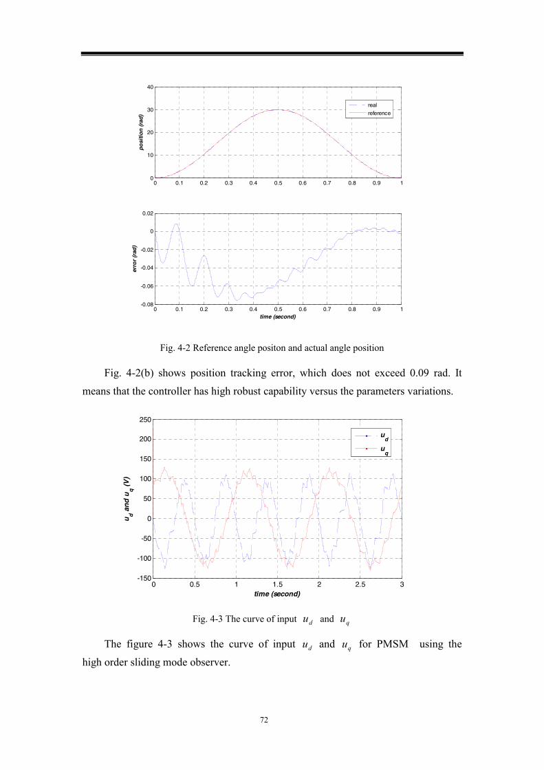
72
0 0.1 0.2 0.3 0.4 0.5 0.6 0.7 0.8 0.9 10
10
20
30
40
po
siti
on
(rad
)
real
reference
0 0.1 0.2 0.3 0.4 0.5 0.6 0.7 0.8 0.9 1-0.08
-0.06
-0.04
-0.02
0
0.02
time (second)
erro
r (r
ad)
Fig. 4-2 Reference angle positon and actual angle position
Fig. 4-2(b) shows position tracking error, which does not exceed 0.09 rad. It
means that the controller has high robust capability versus the parameters variations.
0 0.5 1 1.5 2 2.5 3-150
-100
-50
0
50
100
150
200
250
time (second)
ud a
nd
uq (
V)
ud
uq
Fig. 4-3 The curve of input du and qu
The figure 4-3 shows the curve of input du and qu for PMSM using the
high order sliding mode observer.
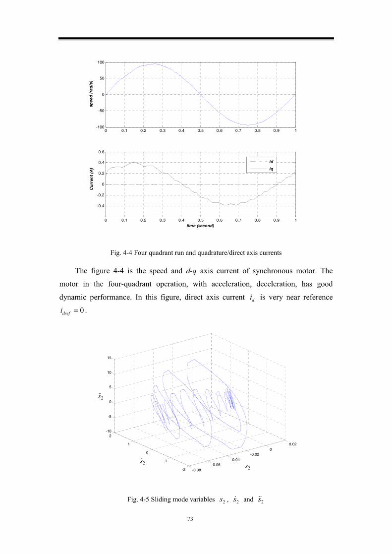
73
0 0.1 0.2 0.3 0.4 0.5 0.6 0.7 0.8 0.9 1-100
-50
0
50
100
spee
d (
rad
/s)
0 0.1 0.2 0.3 0.4 0.5 0.6 0.7 0.8 0.9 1
-0.4
-0.2
0
0.2
0.4
0.6
time (second)
Cu
rren
t (A
)
id
iq
Fig. 4-4 Four quadrant run and quadrature/direct axis currents
The figure 4-4 is the speed and d-q axis current of synchronous motor. The
motor in the four-quadrant operation, with acceleration, deceleration, has good
dynamic performance. In this figure, direct axis current di is very near reference
0=drefi .
-0.08-0.06
-0.04-0.02
00.02
-2
-1
0
1
2-10
-5
0
5
10
15
s2
s2'
s 2''
2s2s
2s
Fig. 4-5 Sliding mode variables 2s , 2s and 2s
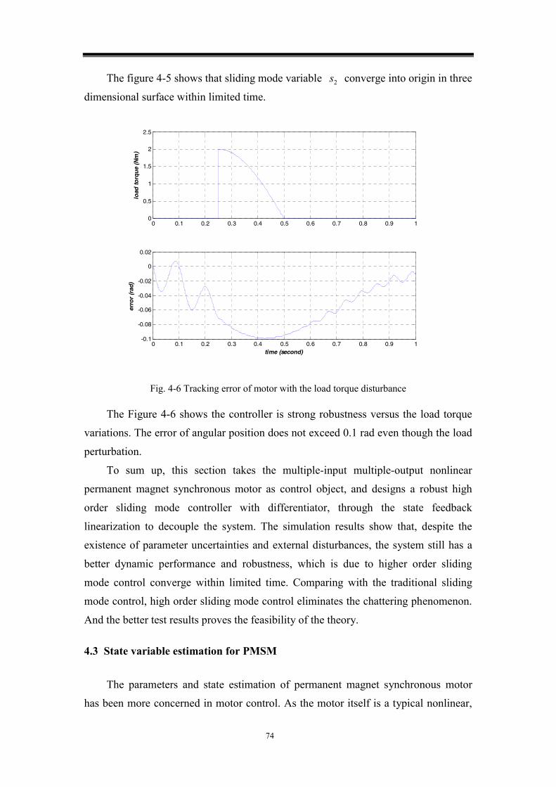
74
The figure 4-5 shows that sliding mode variable 2s converge into origin in three
dimensional surface within limited time.
0 0.1 0.2 0.3 0.4 0.5 0.6 0.7 0.8 0.9 10
0.5
1
1.5
2
2.5lo
ad t
orq
ue
(Nm
)
0 0.1 0.2 0.3 0.4 0.5 0.6 0.7 0.8 0.9 1-0.1
-0.08
-0.06
-0.04
-0.02
0
0.02
time (second)
erro
r (r
ad)
Fig. 4-6 Tracking error of motor with the load torque disturbance
The Figure 4-6 shows the controller is strong robustness versus the load torque
variations. The error of angular position does not exceed 0.1 rad even though the load
perturbation.
To sum up, this section takes the multiple-input multiple-output nonlinear
permanent magnet synchronous motor as control object, and designs a robust high
order sliding mode controller with differentiator, through the state feedback
linearization to decouple the system. The simulation results show that, despite the
existence of parameter uncertainties and external disturbances, the system still has a
better dynamic performance and robustness, which is due to higher order sliding
mode control converge within limited time. Comparing with the traditional sliding
mode control, high order sliding mode control eliminates the chattering phenomenon.
And the better test results proves the feasibility of the theory.
4.3 State variable estimation for PMSM
The parameters and state estimation of permanent magnet synchronous motor
has been more concerned in motor control. As the motor itself is a typical nonlinear,

75
multivariable system with strong coupling, there are a lot algorithms to improve the
motor control performance in recent years. Earlier off-line estimation of the static
dynamic system can not satisfy the control requirements; the use of extended Kalman
filter (EKF) usually have a group of high order nonlinear equations, which is not
conducive to the calculation (Yan,2006), and its stability is also a local stable; In least
squares procedure, the matrix forgotten factor (Poznyak,1999; Poznyak,1999b) is
used to solve non-static parameter identification; as a result of sliding mode control
with strong robustness and global convergence, In recent years, sliding mode observer
(Floret-Pontet,2001; Koshkouei,2002) has been used for dynamic system state and
parameter estimation, but the observer feedback gain is usually not easy to choose.
With the development of nonlinear theory, in order to enhance the performance
of permanent magnet synchronous motor, many advanced control strategies have been
proposed and used in motor control, which requires the state of motor can be
measured, such as mechanical angular position, rotational speed, the electrical current
and so on. Hence mechanical, electromagnetic or photoelectric sensor are needed, as
well known to all, the sensors have many other shortcomings such as drift, friction,
high costs, as well as electromagnetic interference caused by additional conductors.
Therefore, the control system should be as possible as release the use of sensors to
ensure the reliability and stability, which requires the system observer to precisely
estimate the value of the state.
The high order sliding mode control is widely used in last decade, which take
high order derivetives of sliding mode variables to substitute original discrete control,
so that the chattering disappears in the high order differentiation. This section uses a
high order sliding mode observer with differentiator algorithm to estimates the value
of state variables. In this case, it removes the speed and current sensors of motor, and
a better control precision and accurate state estimation are obtained.
In this section, the mathematical model of PMSM is the same with above section
(4.11). In order to make control effectiveness more smooth, the relative order is raised
artificially. Considering control input u as a new input, original sliding mode
variable (4.13) and (4.15) are transformed into
2221212
)4(2
11111
'''''
uBuBAsuBAs
++=
+= (4.28)
Then, the coefficient matrix of original system 1A , 2A , 11B , 21B and 22B
become new matrixes '1A , '2A , '11B , '21B and '22B . Where,
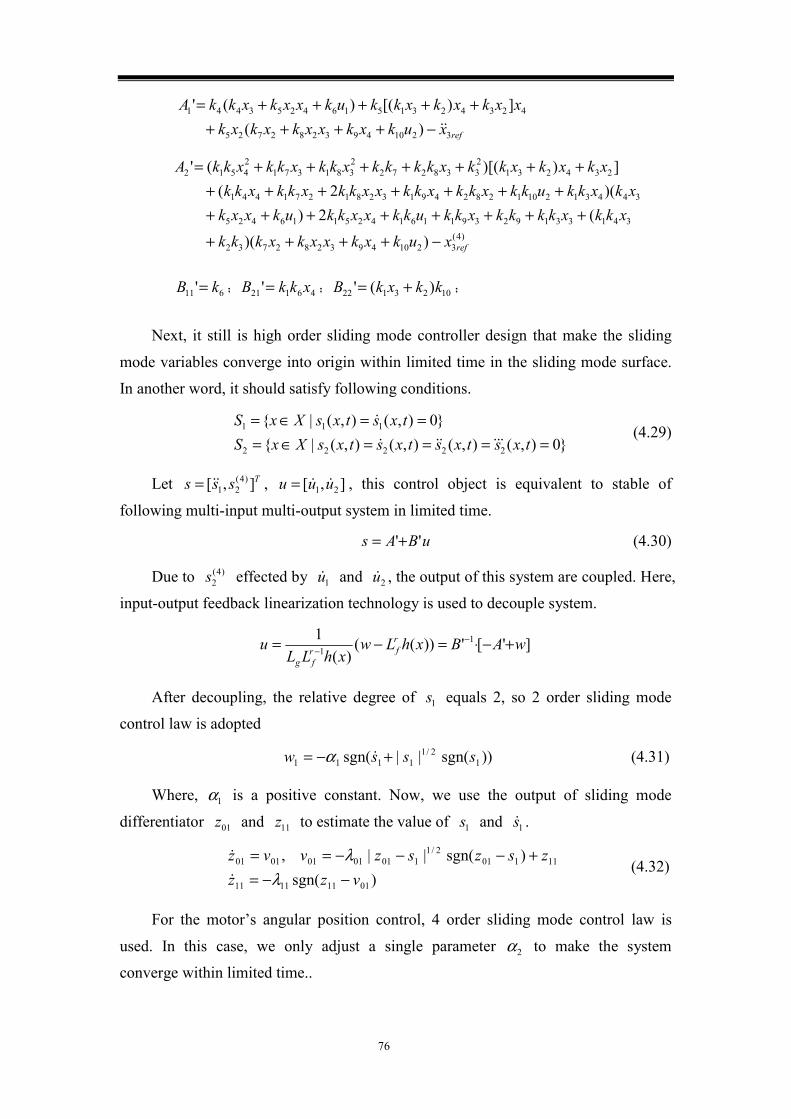
76
refxukxkxxkxkxkxxkxkxkkukxxkxkkA
3210493282725
42342315164253441
)( ])[()('
−+++++++++=
)4(3210493282732
34133192391161425116425
3443121012824913281271441
2342312338272
2381371
24512
))(
(2) )(2(
]))[(('
refxukxkxxkxkkk
xkkxkkkkxkkukkxxkkukxxkxkxkkukkxkkxkkxxkkxkkxkk
xkxkxkkxkkkkxkkxkkxkkA
−++++
++++++++++++++++++++++=
611' kB = ; 46121' xkkB = ; 1023122 )(' kkxkB += ;
Next, it still is high order sliding mode controller design that make the sliding
mode variables converge into origin within limited time in the sliding mode surface.
In another word, it should satisfy following conditions.
}0),(),(),(),(|{
}0),(),(|{
22222
111
====∈===∈=
txstxstxstxsXxStxstxsXxS
(4.29)
Let Tsss ],[ )4(21= , ],[ 21 uuu = , this control object is equivalent to stable of
following multi-input multi-output system in limited time.
uBAs ''+= (4.30)
Due to )4(2s effected by 1u and 2u , the output of this system are coupled. Here,
input-output feedback linearization technology is used to decouple system.
]'['))(()(
1 11 wABxhLw
xhLLu r
frfg
+−⋅=−= −−
After decoupling, the relative degree of 1s equals 2, so 2 order sliding mode
control law is adopted
))sgn(||sgn( 12/1
1111 sssw +−= α (4.31)
Where, 1α is a positive constant. Now, we use the output of sliding mode
differentiator 01z and 11z to estimate the value of 1s and 1s .
)sgn(
)sgn(|| ,
01111111
111012/1
10101010101
vzzzszszvvz
−−=+−−−==
λλ
(4.32)
For the motor’s angular position control, 4 order sliding mode control law is
used. In this case, we only adjust a single parameter 2α to make the system
converge within limited time..
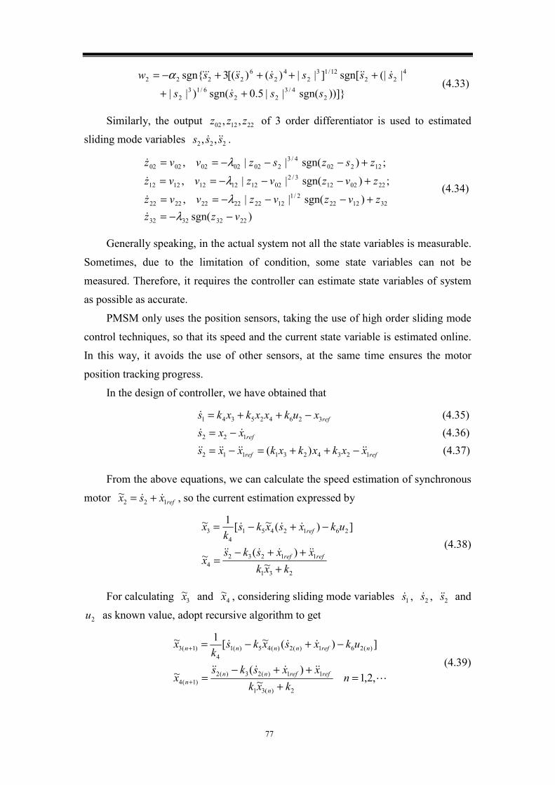
77
))]}sgn(||5.0sgn()||
|(|sgn[]||)()[(3sgn{
24/3
226/13
2
422
12/132
42
62222
ssss
ssssssw
++
++++−= α (4.33)
Similarly, the output 221202 ,, zzz of 3 order differentiator is used to estimated
sliding mode variables 222 ,, sss .
)sgn()sgn(|| ,
;)sgn(|| ,
;)sgn(|| ,
22323232
3212222/1
122222222222
2202123/2
021212121212
122024/3
20202020202
vzzzvzvzvvz
zvzvzvvz
zszszvvz
−−=+−−−==
+−−−==
+−−−==
λλλλ
(4.34)
Generally speaking, in the actual system not all the state variables is measurable.
Sometimes, due to the limitation of condition, some state variables can not be
measured. Therefore, it requires the controller can estimate state variables of system
as possible as accurate.
PMSM only uses the position sensors, taking the use of high order sliding mode
control techniques, so that its speed and the current state variable is estimated online.
In this way, it avoids the use of other sensors, at the same time ensures the motor
position tracking progress.
In the design of controller, we have obtained that
refxukxxkxks 326425341 −++= (4.35)
refxxs 122 −= (4.36)
refref xxkxkxkxxs 1234231112 )( −++=−= (4.37)
From the above equations, we can calculate the speed estimation of synchronous
motor refxsx 122~ += , so the current estimation expressed by
231
112324
26124514
3
~)(~
])(~[1~
kxkxxsks
x
ukxsxksk
x
refref
ref
+++−
=
−+−= (4.38)
For calculating 3~x and 4
~x , considering sliding mode variables 1s , 2s , 2s and
2u as known value, adopt recursive algorithm to get
,2,1 ~
)(~
])(~[1~
2)(31
11)(23)(2)1(4
)(261)(2)(45)(14
)1(3
=+
++−=
−+−=
+
+
nkxk
xxsksx
ukxsxksk
x
n
refrefnnn
nrefnnnn
(4.39)

78
Where, n is the n th sample point of system, 1+n is the next sample point.
Through the above recursive equation, current estimation 3~x and 4
~x are obtained.
Take these estimation into the control system so that save the sensors. Thereby,
system become more simple and reliability.
In the simulation, we use the DutyMAX95-BSC060300 permanent magnetic
synchronous motor. The parameters of motor are 3=P , smNB ⋅⋅= 0034.0 ,
Ω= 3.3R , HLd 027.0= , HLq 0034.0= , Wbf 341.0=ψ , 20037.0 mkgJ ⋅= . A phase
current of the maximum accepted value is A0.6 , the load torque maximum value is
mN ⋅6 , and angular velocity is rpm3000 .
The parameter of controller are 51 =α and 502 =α ; the parameter of sliding
mode differentiator are 201 =λ , 5.111 =λ , 2502 =λ , 2512 =λ , 3322 =λ and
50032 =λ .
From the figure 4-7(a) we can see that the permanent magnet synchronous motor
control system has good performance. This figure shows the permanent magnet
synchronous motor can precisely track the given position. And the error between
reference and the actual position feedback is shown in Figure 4-7(b) below. The
maximal error does not exceed to 0.08 rad.
0 1 2 3 4 5 6 7 8 9 100
10
20
30
posi
tion
(rad
)
a
real
reference
0 1 2 3 4 5 6 7 8 9 10-0.08
-0.06
-0.04
-0.02
0
0.02
time (second)
erro
r (r
ad)
Fig. 4-7 Position tracking and error curve of PMSM

79
0 1 2 3 4 5 6 7 8 9 10-10
-5
0
5
10
spee
d (r
ad/s
)
(a)
0 1 2 3 4 5 6 7 8 9 10-0.1
-0.05
0
0.05
0.1
erro
r (r
ad/s
)
time (second)
(b)
Fig. 4-8 Speed estimation and error curve of PMSM
The figure 4-8(a) shows the motor angular speed by derivative of the motor’s
angular position. The figure 4-8(b) shows the error between the estimation of the
electrical angular speed and the value calculated by the formula (4.36).
0 5 10-0.02
0
0.02
id-e
stim
atio
n (A
) (a)
0 5 10-0.04
-0.02
00.020.04
iq-e
stim
atio
n (A
) (b)
0 5 10-0.02
0
0.02
id (
A)
(c)
0 5 10-0.04-0.02
00.020.04
iq (
A)
(d)
0 5 10-1
0
1x 10
-4
time (second)
erro
r (A
)
(e)
0 5 10-2
0
2x 10
-3
time (second)
erro
r (A
)
(f)
Fig. 4-9 The quadrature/direct axis currents and their estimations

80
For permanent magnet synchronous motor, its angular position, speed and
current are system state values. The figure 4-9(a), (b), (c), (d) shows that the estimated
value and actual current value of direct axis and quadrature axis respectively. The
figure 4-9(e), (f) are the error between actual current value and the estimated value. In
this figure, the error of direct axis current is between )(100.1 4 A−×± , and the error of
quadrature axis is between )(100.1 3 A−×± .
0 5 10-0.08
-0.06
-0.04
-0.02
0
0.02
s
0 5 10-0.3
-0.2
-0.1
0
0.1
s'
0 5 10-4
-3
-2
-1
0
1
time (second)
s''
0 5 10-30
-20
-10
0
10
20
30
time (second)
s(3)
s s
s s
Fig. 4-10 System sliding mode variables curve
The figure 4-10 is the convergence curve of sliding mode variable and its high
order derivatives. From the figure we can clearly see that the discrete control law acts
on the high order sliding mode surface, which makes the lower sliding mode surface
smooth. That is the reason why high order sliding mode control can eliminate the
chattering.
This subsection focuses on a state estimation of PMSM online. In the practical
systems, not all the state variables are measurable, or because of objective reasons
they are often not easy to measure. In this section, we just use the motor position
sensor, through the high order sliding mode control with differentiator, to achieve the
state variables of motor estimation online. The simulation results show that the
PMSM control system has good dynamic performance, while the electrical angular
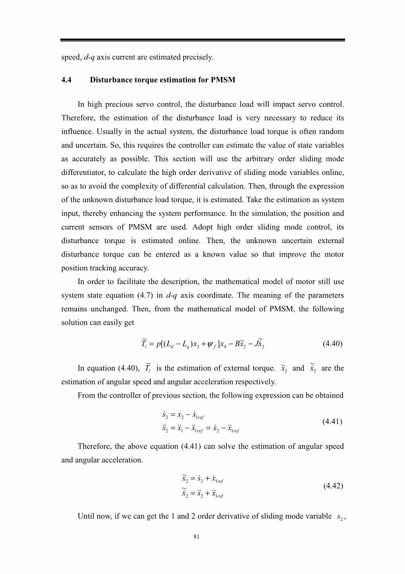
81
speed, d-q axis current are estimated precisely.
4.4 Disturbance torque estimation for PMSM
In high precious servo control, the disturbance load will impact servo control.
Therefore, the estimation of the disturbance load is very necessary to reduce its
influence. Usually in the actual system, the disturbance load torque is often random
and uncertain. So, this requires the controller can estimate the value of state variables
as accurately as possible. This section will use the arbitrary order sliding mode
differentiator, to calculate the high order derivative of sliding mode variables online,
so as to avoid the complexity of differential calculation. Then, through the expression
of the unknown disturbance load torque, it is estimated. Take the estimation as system
input, thereby enhancing the system performance. In the simulation, the position and
current sensors of PMSM are used. Adopt high order sliding mode control, its
disturbance torque is estimated online. Then, the unknown uncertain external
disturbance torque can be entered as a known value so that improve the motor
position tracking accuracy.
In order to facilitate the description, the mathematical model of motor still use
system state equation (4.7) in d-q axis coordinate. The meaning of the parameters
remains unchanged. Then, from the mathematical model of PMSM, the following
solution can easily get
2243~~])[(~ xJxBxxLLpT fqdl −−+−= ψ (4.40)
In equation (4.40), lT~ is the estimation of external torque. 2~x and 2
~x are the
estimation of angular speed and angular acceleration respectively.
From the controller of previous section, the following expression can be obtained
refref
ref
xxxxsxxs
12112
122
−=−=
−= (4.41)
Therefore, the above equation (4.41) can solve the estimation of angular speed
and angular acceleration.
ref
ref
xsx
xsx
122
122
~~
+=
+= (4.42)
Until now, if we can get the 1 and 2 order derivative of sliding mode variable 2s ,
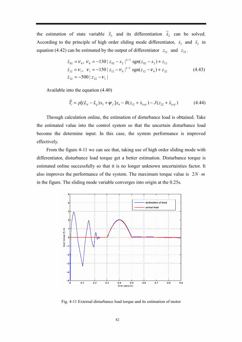
82
the estimation of state variable 2~x and its differentiation 2
~x can be solved.
According to the principle of high order sliding mode differentiator, 2s and 2s in
equation (4.42) can be estimated by the output of differentiator 12z and 22z .
||500
)sgn(||150 ,
)sgn(||130 ,
12222
220122/1
0121112
122023/2
2020002
ννννν
νν
−−=+−−−==
+−−−==
zzzzzz
zszszz
(4.43)
Available into the equation (4.40)
)()(])[(~12211243 refreffqdl xzJxzBxxLLpT +−+−+−= ψ (4.44)
Through calculation online, the estimation of disturbance load is obtained. Take
the estimated value into the control system so that the uncertain disturbance load
become the determine input. In this case, the system performance is improved
effectively.
From the figure 4-11 we can see that, taking use of high order sliding mode with
differentiator, disturbance load torque get a better estimation. Disturbance torque is
estimated online successfully so that it is no longer unknown uncertainties factor. It
also improves the performance of the system. The maximum torque value is mN ⋅2
in the figure. The sliding mode variable converges into origin at the 0.25s.
Fig. 4-11 External disturbance load torque and its estimation of motor
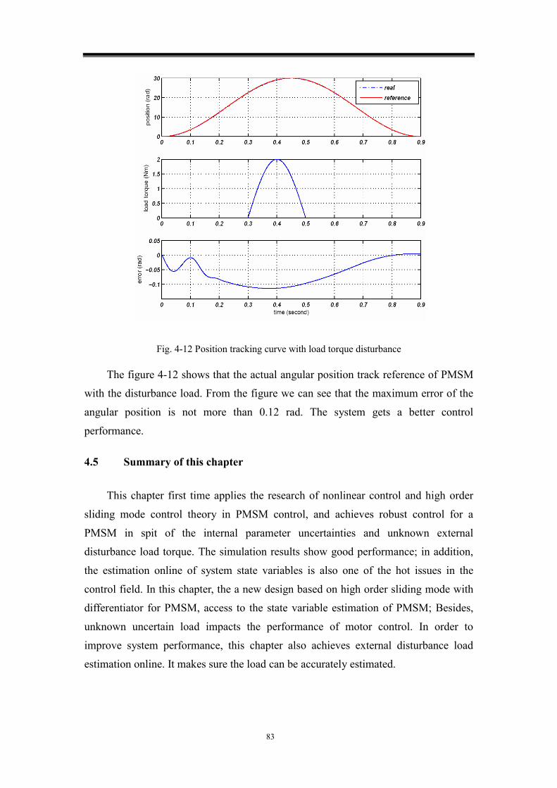
83
Fig. 4-12 Position tracking curve with load torque disturbance
The figure 4-12 shows that the actual angular position track reference of PMSM
with the disturbance load. From the figure we can see that the maximum error of the
angular position is not more than 0.12 rad. The system gets a better control
performance.
4.5 Summary of this chapter
This chapter first time applies the research of nonlinear control and high order
sliding mode control theory in PMSM control, and achieves robust control for a
PMSM in spit of the internal parameter uncertainties and unknown external
disturbance load torque. The simulation results show good performance; in addition,
the estimation online of system state variables is also one of the hot issues in the
control field. In this chapter, the a new design based on high order sliding mode with
differentiator for PMSM, access to the state variable estimation of PMSM; Besides,
unknown uncertain load impacts the performance of motor control. In order to
improve system performance, this chapter also achieves external disturbance load
estimation online. It makes sure the load can be accurately estimated.
84
Chapter 5 Experimental system based on dSPACE
dSPACE is a equipment of control exploitation and test system based on
MATLAB/Simulink that is from Germany. It implements seamless link with the
MATLAB/Simulink completely. It can complete the control algorithm design, test and
implementation, overcoming the shortage of the traditional control system, for
example, the difficult to achieve the complex algorithm and the long development
cycle. It has advantages of high speed, ease to use and user-friendly.
This chapter is structured as follows: 5.1, introduce the basic functions of the
dSPACE real time control platform; 5.2, design a permanent magnet synchronous
motor control system based the dSPACE; 5.3, describe development process of the
control system in detail; 5.4 experiment results confirm the feasibility of high order
sliding mode control for the nonlinear permanent magnet synchronous motor, and
compared with the traditional sliding mode control; 5.5, Summary of this chapter.
5.1 Introduction of dSPACE control platform
In the design and development process of permanent magnet synchronous motor
control system, the traditional digital/analog circuit exist the following questions:
(1) In the situation of the control law or control features not yet fully grasped, if
the hardware circuit has been manufactured, but do not know whether the program
can satisfy the requirements, it will result in a waste of hardware costs;
(2) As a result of manual programming, so the code would have the unreliable
problem. If in the course of test, it is difficult to determine the fault reason due to
unsatisfactory control program or software code with an error;
(3) Even if the software does not exist, if control program is not satisfactory,
needed for modification, both of hardware and software must be revised. It is based
on the above considerations, a high-tech company in Germany dSPACE provides
hardware and software platform for development and test of control projects.
Due to the dSPACE with the powerful real time systems, it can be connected to
the actual control object (known as rapid control prototyping), when it played the role
of the main controller; and can be connected to the actual controller (known as
hardware-in-the-loop simulation), when it played the role of the object. Thus the
development cycle is shorted and the development cost is reduced, which based on the
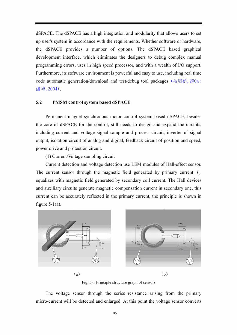
85
dSPACE. The dSPACE has a high integration and modularity that allows users to set
up user's system in accordance with the requirements. Whether software or hardware,
the dSPACE provides a number of options. The dSPACE based graphical
development interface, which eliminates the designers to debug complex manual
programming errors, uses in high speed processor, and with a wealth of I/O support.
Furthermore, its software environment is powerful and easy to use, including real time
code automatic generation/download and test/debug tool packages (马培蓓,2004;
潘峰,2004).
5.2 PMSM control system based dSPACE
Permanent magnet synchronous motor control system based dSPACE, besides
the core of dSPACE for the control, still needs to design and expand the circuits,
including current and voltage signal sample and process circuit, inverter of signal
output, isolation circuit of analog and digital, feedback circuit of position and speed,
power drive and protection circuit.
(1) Current/Voltage sampling circuit
Current detection and voltage detection use LEM modules of Hall-effect sensor.
The current sensor through the magnetic field generated by primary current pI
equalizes with magnetic field generated by secondary coil current. The Hall devices
and auxiliary circuits generate magnetic compensation current in secondary one, this
current can be accurately reflected in the primary current, the principle is shown in
figure 5-1(a).
(a) (b)
Fig. 5-1 Principle structure graph of sensors
The voltage sensor through the series resistance arising from the primary
micro-current will be detected and enlarged. At this point the voltage sensor converts
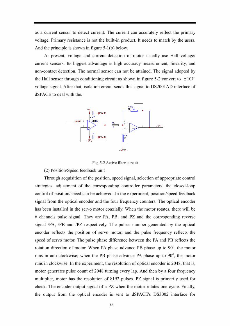
86
as a current sensor to detect current. The current can accurately reflect the primary
voltage. Primary resistance is not the built-in product. It needs to match by the users.
And the principle is shown in figure 5-1(b) below.
At present, voltage and current detection of motor usually use Hall voltage/
current sensors. Its biggest advantage is high accuracy measurement, linearity, and
non-contact detection. The normal sensor can not be attained. The signal adopted by
the Hall sensor through conditioning circuit as shown in figure 5-2 convert to V10±
voltage signal. After that, isolation circuit sends this signal to DS2001AD interface of
dSPACE to deal with the.
Fig. 5-2 Active filter curcuit
(2) Position/Speed feedback unit
Through acquisition of the position, speed signal, selection of appropriate control
strategies, adjustment of the corresponding controller parameters, the closed-loop
control of position/speed can be achieved. In the experiment, position/speed feedback
signal from the optical encoder and the four frequency counters. The optical encoder
has been installed in the servo motor coaxially. When the motor rotates, there will be
6 channels pulse signal. They are PA, PB, and PZ and the corresponding reverse
signal /PA, /PB and /PZ respectively. The pulses number generated by the optical
encoder reflects the position of servo motor, and the pulse frequency reflects the
speed of servo motor. The pulse phase difference between the PA and PB reflects the
rotation direction of motor. When PA phase advance PB phase up to 90o, the motor
runs in anti-clockwise; when the PB phase advance PA phase up to 90o, the motor
runs in clockwise. In the experiment, the resolution of optical encoder is 2048, that is,
motor generates pulse count of 2048 turning every lap. And then by a four frequency
multiplier, motor has the resolution of 8192 pulses. PZ signal is primarily used for
check. The encoder output signal of a PZ when the motor rotates one cycle. Finally,
the output from the optical encoder is sent to dSPACE's DS3002 interface for
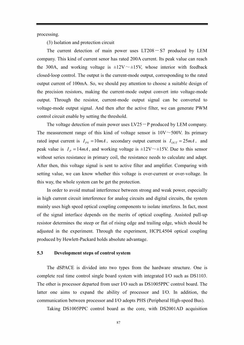
87
processing.
(3) Isolation and protection circuit
The current detection of main power uses LT208-S7 produced by LEM
company. This kind of current senor has rated 200A current. Its peak value can reach
the 300A, and working voltage is ±12V~±15V, whose interior with feedback
closed-loop control. The output is the current-mode output, corresponding to the rated
output current of 100mA. So, we should pay attention to choose a suitable design of
the precision resistors, making the current-mode output convert into voltage-mode
output. Through the resistor, current-mode output signal can be converted to
voltage-mode output signal. And then after the active filter, we can generate PWM
control circuit enable by setting the threshold.
The voltage detection of main power uses LV25-P produced by LEM company.
The measurement range of this kind of voltage sensor is 10V~500V. Its primary
rated input current is mAIPN 10= , secondary output current is mAIOUT 25= , and
peak value is mAI P 14= , and working voltage is ±12V~±15V. Due to this sensor
without series resistance in primary coil, the resistance needs to calculate and adapt.
After then, this voltage signal is sent to active filter and amplifier. Comparing with
setting value, we can know whether this voltage is over-current or over-voltage. In
this way, the whole system can be get the protection.
In order to avoid mutual interference between strong and weak power, especially
in high current circuit interference for analog circuits and digital circuits, the system
mainly uses high speed optical coupling components to isolate interferes. In fact, most
of the signal interface depends on the merits of optical coupling. Assisted pull-up
resistor determines the steep or flat of rising edge and trailing edge, which should be
adjusted in the experiment. Through the experiment, HCPL4504 optical coupling
produced by Hewlett-Packard holds absolute advantage.
5.3 Development steps of control system
The dSPACE is divided into two types from the hardware structure. One is
complete real time control single board system with integrated I/O such as DS1103.
The other is processor departed from user I/O such as DS1005PPC control board. The
latter one aims to expand the ability of processor and I/O. In addition, the
communication between processor and I/O adopts PHS (Peripheral High-speed Bus).
Taking DS1005PPC control board as the core, with DS2001AD acquisition

88
board, DS2002/2003 multi-channel AD acquisition board, CP4002 Multi-I/O board,
DS2102DA output board, DS3002 incremental encoder interface board, we constitute
a standard component hardware parts of dSPACE DS1005 system, which is used in
this experiment.
After the completion of the experimental platform, the development steps of
control system for PMSM based on the dSPACE include the following points:
(1) MATLAB/Simulink modeling and off-line simulation. Take use of
MATLAB/Simulink to establish a mathematical model for the simulation object, and
design control programs. At the same time, complete the system off-line simulation.
(2) Input/output interface (I/O) experimental model. In the MATLAB/Simulink
environment, we need to retain module that is downloaded to the dSPACE. Select the
real-time control required for I/O modules from the RTI library. Replace the original
connection relationship with the hardware interface, and configure I/O parameters. In
some special cases, we also need to set up hardware and software interrupt priority
levels.
Fig. 5-6 MATLAB/Simulink environment based on dSPACE/RTI control system
The figure 5-6 is a control system in MATLAB/Simulink environment with the

89
dSPACE/RTI module. In detail, PWM interface RTI modules produce a variety of
optional items depending on the PWM methods. The PWM output has 8-channel at
most. But for the three phase motor, we only need to select the 3-channel PWM
interface RTI module from DS4002PWM3_OUT. Usually, motor speed can be
obtained by coaxial encoder. The RTI module DS3002POS_B1_C1 can get the
position and delta position signals. The module of DS3002HW_INDEX_B1_C1 can
get a zero-position signal. Due to the requirement of current and voltage sample, we
use the AD interface DS2001_B1/ DS2002_B1 /DS2003_B1. Among them,
DS2001_B1 can sample 5-channel analog signal (±5V or ±10V) at the same time. In
addition, for the output analog signals, we can use the DA interface DS2102_B1 that
creates analog signals (±5V, ±10V or 0~10V) easily. It's worth noting that the output
value ±1 of MATLAB/Simulink corresponds analog output ±5V or ±10V, and the
output value 0~1 corresponds analog output 0~10V.
(3) The dSPACE/RTW provides tools to automatically generate code and
download. Since MATLAB and dSPACE with seamless connectivity features, a
simple operation can complete real-time C code generation, compile, link and
download for the target system. In other word, model is downloaded into target board
DS1005PPC as running program.
(4) The dSPACE integrated experiment and debugging. The dSPACE provides
real-time ControlDesk software as well, which changes the parameters and real-time
control.
5.4 Experiment results and analysis
I. Content and intention:
1. Validate feasibility of high order sliding mode control in PMSM;
2. Test system using high sliding mode control whether it can release chattering
phenomenon;
3. Test system using high sliding mode control whether it has robustness.
II. Equipments:
Name Type Unit Amount
dSPACE controller DS1005 Dais 1
DC regulated power WYK-303B2 Dais 1
90
Slide-wire rheostat BX8D-3/7 Dais 3
Switch regulated power S-100-24 Dais 1
Universal meter LINI-T/UT58A Dais 1
Ondoscope Tektronix/TDS2024 Dais 1
Industrial computer ADLINK Dais 1
III. Experimental procession:
Step 1: Off-line simulation. According to the principle of high order sliding mode
control and differentiator, combining with chapter 5 of the application for permanent
magnet synchronous motor, the theoretical simulation is researched in the
MATLAB/Simulink firstly. In detail, set the sampling frequency and differential
equation solution, and save the .mdl model file;
Step 2: After the control algorithm verification, remove the inverter model and
motor model replaced by the physical prototypes of actual system. And then complete
all of the system interface, including the A /D, D/A, I/O, PWM and other interfaces of
the dSPACE. Afterwards, compile on-line to generate. cof configuration file;
Step 3: Check all connections are correct. After that, start the dSPACE. Compile
and download files real-time (RTI) in the environment of MATLAB/Simulink. At this
moment, algorithm program code is downloaded to the DSP core program area of
dSPACE controller;
Step 4: Start the dSPACE/ControlDesk. Create an experimental file .prj in the
interface, and design the required .lay layer file. Observe compiler-generated variable
file .sdf in order to facilitate observe the real-time dynamic performance of the
system;
Step 5: After the completion of the above, check the status of external devices is
good or not. Finally, start bus power, while start system operation in
dSPACE/ControlDesk interface.
IV. Controlled device:
The controlled object in experiments uses non-salient pole permanent magnet
synchronous motor of Delta's ASMT series, whose main parameters are as follows
Table 5-1:
Tab. 5-1 Parameters of PMSM in experiment
91
Name Resistance Inductance Rating Power Torque
Value 052.2=R 4.8=L 0.1=P 3.3=T
Unit Ω mH kW mN ⋅
Name Pole-pairs Voltage Speed Rotary inertia
Value 4=pN 300=U 3000=Nn 00026.0=J
Unit —— V min/r 2mkg ⋅
Host-computer control surface adopts visual man-machine surface the
dSPACE/ControDesk to realize data acquisition and display. Fig. 5-8 is pictorial
diagram based on the dSPACE control system. The system consists of inverter,
isolation circuit, detection circuit, power circuit and etc.
Fig. 5-8 Control system hardware circuit with dSPACE interface
V. Waveform:
Because the research of nonlinear system high order sliding mode control theory
still is in primary stage, it is face with much challenge. For example, it strictly
requires all of the system functions are smooth, and norm-bounded. Otherwise, there
is the higher derivative of reference value in control law. In our experiment, 60V DC
regulated power is supplied. Experiment is tested under the conditions above. The
main test results are following.
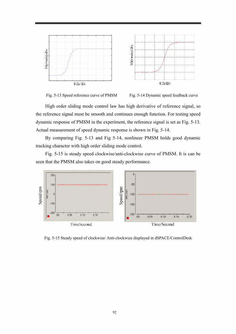
92
Fig. 5-13 Speed reference curve of PMSM Fig. 5-14 Dynamic speed feedback curve
High order sliding mode control law has high derivative of reference signal, so
the reference signal must be smooth and continues enough function. For testing speed
dynamic response of PMSM in the experiment, the reference signal is set as Fig. 5-13.
Actual measurement of speed dynamic response is shown in Fig. 5-14.
By comparing Fig. 5-13 and Fig 5-14, nonlinear PMSM holds good dynamic
tracking character with high order sliding mode control.
Fig. 5-15 is steady speed clockwise/anti-clockwise curve of PMSM. It is can be
seen that the PMSM also takes on good steady performance.
Fig. 5-15 Steady speed of clockwise/ Anti-clockwize displayed in dSPACE/ControlDesk
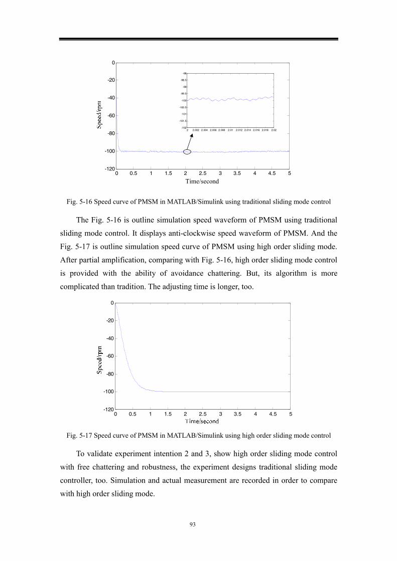
93
0 0.5 1 1.5 2 2.5 3 3.5 4 4.5 5-120
-100
-80
-60
-40
-20
0
? ? /?
?/?
?
2 2.002 2.004 2.006 2.008 2.01 2.012 2.014 2.016 2.018 2.02-102
-101.5
-101
-100.5
-100
-99.5
-99
-98.5
-98
? ? /?
?/?
?
Time/second
Fig. 5-16 Speed curve of PMSM in MATLAB/Simulink using traditional sliding mode control
The Fig. 5-16 is outline simulation speed waveform of PMSM using traditional
sliding mode control. It displays anti-clockwise speed waveform of PMSM. And the
Fig. 5-17 is outline simulation speed curve of PMSM using high order sliding mode.
After partial amplification, comparing with Fig. 5-16, high order sliding mode control
is provided with the ability of avoidance chattering. But, its algorithm is more
complicated than tradition. The adjusting time is longer, too.
0 0.5 1 1.5 2 2.5 3 3.5 4 4.5 5-120
-100
-80
-60
-40
-20
0
? ? /?
?/?
?
Fig. 5-17 Speed curve of PMSM in MATLAB/Simulink using high order sliding mode control
To validate experiment intention 2 and 3, show high order sliding mode control
with free chattering and robustness, the experiment designs traditional sliding mode
controller, too. Simulation and actual measurement are recorded in order to compare
with high order sliding mode.

94
Fig. 5-18 Speed curve in dSPACE/ControlDesk using traditional (high order) sliding mode control
Due to the traditional sliding mode control uses discontinues control law acting
on sliding mode manifold surface, chattering problem is caused. The great of the
coefficient in sliding mode control law, the faster of convergence, when the system
enter into sliding mode, chattering phenomenon is more obvious. Fig. 5-18(a) is
actual measurement speed curve of PMSM, which adopts conventional sliding mode
control. The control law is sKu i sgn−= , in current loop 51 =K , in speed loop
2.82 =K . From the Fig. 5-18, we can obtain a conclusion that chattering is released
in high order sliding mode.
Hereto, both of simulation and experiment results prove that high order sliding
mode control can reduce the chattering phenomenon which exists in conventional.
Following experiment will test the robustness of high order sliding mode control.
time/second
Load
Fig. 5-19 Speed curve of 0.5 mN ⋅ disturbance load in dSPACE/ControlDesk
The PMSM is a typical complex system because of elevated temperature,
saturation, time delay and a good many elements. These reasons lead to the
synchronous motor is nonlinear, variation parameter, close coupled system. For the
sake of testing high order sliding control, which is insensitive to the parameter

95
uncertainness and disturbance, experiment is injected about 0.5 mN ⋅ external load
disturbance at the 0.01 second. The speed actual measurement waveform is shown in
Fig. 5-19. From this figure, speed curve is smooth without flutter. The experiment
result illuminates high order sliding mode control reserves robustness of conventional
sliding mode.
Experimentally verified, high order sliding mode control provides an effective
method to improve accuracy and robustness further for nonlinear systems.
5.5 Summary of this chapter
This chapter first described dSPACE physics experiment control platform the
build and development process in detail. Through the dSPACE real-time control
platform, the nonlinear high order sliding mode control theory research is applied to
the control of permanent magnet synchronous motor. The experimental results and
simulation results are consistently indicate that synchronous motor has better dynamic
performance and steady accuracy, proves the feasibility of this technology in practical
application systems; It is also verified by high order sliding mode control technique
that preserves the robustness of traditional sliding mode control. The high order
sliding mode essentially eliminates the chattering caused by discrete control law.
From another point of view, the simulation and physical experiment provide a certain
reference value for the nonlinear systems high order sliding mode control further
application.
96
Chapter 6 Summary
This paper focuses on the nonlinear system control theory and high order sliding
mode control theory. The exact feedback linearization technology of nonlinear
systems needs to be applied under the accurate model of the technical requirements,
which is not easy to achieve in the actual system. High order sliding mode control
technology preserves the strong robustness of the traditional sliding mode control,
which is not sensitive to the uncertain parameters of systemic model and the unknown
external disturbances. But in comparison with the traditional sliding mode control,
high order sliding mode control technique uses high order differential of sliding mode
variable to transfer the chattering phenomenon generated in discontinuous discrete
control into higher order sliding surface, making the low order sliding surface
eliminate the chattering and improving the control precision. Considered all above
together, this paper will organically integrate nonlinear control and high order sliding
mode control with their full strengths to improve the overall performances of system.
For permanent magnet synchronous motor is a typical MIMO nonlinear system, we
conduct a high order sliding mode control experiment, mainly including the research
areas of servo control, robustness, state estimation and disturbance estimation so that
it can get a better good application effect.
6.1 The chief work and research results of the paper
1. As the differential geometry theory is based on precise mathematical models,
but in the actual system the uncertain system parameters and the unknown external
disturbances can not be avoided, so the application of exact feedback linearization
theory has been somewhat restricted. In this paper, use the robustness of sliding mode
control on parameter uncertainty and external disturbance to design a high order
sliding mode controller with the combination of exact linearization theory. It can not
only eliminate the chattering in traditional sliding mode control and improve the
control precision, but also circumvent the application condition that the relevant
degree requirement is stringently equal to 1.
2. In the design of high order sliding mode controller, we often need to know
the arbitrary order derivative of sliding variable values, so how to get each variable
differential becomes considerable complex and cumbersome. This paper presents an
97
arbitrary order differentiator designed by high order sliding mode observer, which can
avoids the large number of numerical method calculation. From the application
example, it can be seen that the differentiator is not only high accurate but also strong
robust. This paper will also use the differentiator to apply to the on-line observation of
MIMO nonlinear system state and input variables, and consequently get more ideal
control effect. This lays the foundation for the next application of the actual system.
3. For permanent magnet synchronous motor commonly used in industrial
control, taking into account its nonlinear characteristics and the strong coupling
relationship between multiple variables of the system as well as the impact of the
working environment, this paper designs a robust high order sliding mode controller
applied to permanent magnet synchronous motor at the first time. First, it conducts the
exact feedback linearization to the mathematical model of nonlinear MIMO motor
and achieves a decoupling control. In this way, the design of complex nonlinear
systems is converted to control a number of SISO linear subsystems so that control
objectives are easy to implement. Then, based on high order sliding mode control
theory, it designs the double closed-loop robustness controller in position and current
for permanent magnet motor. Through the simulation, it can be seen the position
tracking of the system tracks with high precision and the maximum error is only
0.09rad. Although there are some factors such as the parameter uncertainty and
external unknown torque disturbance in the system, it still has a strong robustness. In
addition, chattering phenomenon has been significantly ameliorated after the
application of higher order sliding mode controller.
4. Taking into account that the arbitrary order sliding mode differentiator has
the role of observer, this paper uses sliding mode differentiator to construct on-line
accurate observation on the motor state variables for the permanent magnet
synchronous motor at the first time. The sliding mode observer is designed to achieve
the observation on motor speed, d-q axis current state variables. From another
viewpoint, the value of state variable feedback for motor controller can not be
obtained only through sensors but be directly obtained from the output of the
observations. Thus it eliminates the effect of mechanical or electronic sensors,
reducing the cost and improving the reliability of the system. Simulation results show
that the high order sliding mode controller with differentiator, its speed and current
values are observed with high accuracy.
5. In the motor control technologies, we often encounter the external unknown
98
and uncertain disturbances. The most primary is the external load torque which poses
a severe challenge to the system control performances. The application of robustness
control techniques has become the studying hot point. This thesis uses high order
sliding mode observer to present on-line estimate expression of external torque.
Through the real-time calculation of the expression, we can estimate the more
accurate value of disturbance torque by using high order sliding mode differentiations
and related system variable values. As a result, the external disturbance signal of
system is no longer unknown but can be accurately estimated. Therefore, the system’s
capacity to resist external disturbances has further improved.
6. In order to verify the simulation results, this paper adopts dSPACE
semi-physical simulation experimental platform to complete the physical experiment
at last. Through the results from the MATLAB/Simulink simulation, the system
downloads software programs of nonlinear high order sliding mode control algorithm
into the memorizer of dSPACE's subordinate computer in order to control the motor
drivers to work, and ultimately it achieves on-line and real-time experiment of
synchronous motor. Experimental results show the high order sliding mode control
theory of nonlinear systems can be successfully applied to permanent magnet
synchronous motor control system. The method not only retains the robustness of
traditional sliding mode control, but also effectively eliminates the chattering
problems in the traditional sliding mode control. This lays the foundation for the
widespread application in the future.
6.2 Several issues to be resolved
The study of nonlinear system control theory is one difficult and challenging
topic in present control theories. And the sliding mode control of nonlinear system
develops at the initial stage. In terms of high order sliding mode control of nonlinear
system studied in this paper, there are still some important issues need to be explored
and further studied.
1. Nonlinear control is a subject with relatively broad range and rather deep
content. This paper focuses on the affine and matching high order sliding mode
control of nonlinear system. For non-affine or non-matching non-linear systems, it
doesn’t carry out study, which is to be in-depth study area for nonlinear sliding mode
control.
2. The application of quasi-continuous high order sliding mode control

99
technique with smooth control law has not yet been generalized, because the theory
itself has certain limitations. Its core idea is to minimize discrete sign function items
in the control law. But for some specific practical systems, it is possible to appear
uncertain items when the denominator of control law approaches zero. Nevertheless,
this idea is still very useful, which is the problem to be solved in the future.
3. It is well known that using sliding mode control with differentiator can
achieve state estimation and external disturbance estimation for nonlinear permanent
magnet synchronous motor. With the thought, it should also be able to achieve the
on-line parameter identification of system. In the simulation experiments, it’s showed
that the stator resistances as well as the value of motor flux can be better identified.
For motors, the inductance is undoubtedly a more important parameter. However, the
inductance identification results found in many simulation experiments were
unsatisfactory. It is due to under normal circumstances the unit of the electrical
inductance is millihenry, when we use sliding mode variable and relevant state
variables to estimate it, occurring a zero-zero phenomenon. Specifically, when the
sliding variable is converging to zero in finite time, the molecular and denominator of
the inductance are also converging to zero. Thus, the identification reliability of the
method remains to be further studied.
4. High order sliding mode control technology with higher control accuracy
essentially eliminates the chattering phenomenon and keeps the robustness of the
traditional sliding mode control. However, a fly in the ointment is that the technology
needs to seek high order derivatives under a given reference value. So a given
function is required to be continuously differentiable everywhere in the time domain.
In fact, that is much harsher in a real system. Therefore, how to relax the using
conditions is also an important research area for high order sliding mode control
technology.

100
Reference
[Baik,1998] I. C. Baik, K. H. Kim and M. Y. Youn. Robust nonlinear speed control of
PM synchronous motor using adaptive and sliding mode control techniques[J]. IEEE
Proceedings of Electrical Power Application, vol. 145(4), pp. 369–375, 1998
[Bartolini,1997] G. Bartolini, A. Ferrara and E. Usai. Application of a sub-optimal
discontinuous control algorithm for uncertain second order systems[J]. International
Journal of Robust and Nonlinear Control, Vol. 7, 299-319, 1997
[Bartolini,1998] G. Bartolini, A. Ferrara and E. Usai. Chattering avoidance by second
order sliding mode control[J]. IEEE Transactions on Automatic Control, Vol. 43(2),
241-246, 1998
[Bartolini,1998b] G. Bartolini, M. Coccoli and A. Ferrara. Vibration damping and
second order sliding modes in the control of a single finger of the AMADEUS
gripper[J]. International Journal of Systems Science, Vol. 29(5), 497-512, 1998
[Bartolini,1998c] G. Bartolini, A. Ferrara, A. Levant and Usai E. On second order
sliding mode controllers[J]. Processing of 5th International Workshop on VSS,
Longboat Key, Florida. 1998
[Bartolini,1999] G. Bartolini, A. Ferrara and Giacomini. A robust control design for a
class of uncertain nonlinear systems featuring a second order sliding mode[J].
International Journal of Control, Vol. 72(4), 321-331, 1999
[Bartolini,1999b] G. Bartolini, A. Levant, E. Usai and A. Pisano. 2-Sliding Mode with
Adaptation[J]. Proceedings of the 7th Mediterranean Conference on Control and
Automation, pp. 2421–2429, 1999
[Bartolini,2000] G. Bartolini, A. Ferrara and E. Punta. Multi-input second order
sliding mode hybrid control of constrained manipulators[J]. Dynamics and Control,
Vol. 10, 277-296, 2000
[Bartolini,2000b] G. Bartolini, A. Ferrara and E. Usai and V.I. Utkin. On multi-input
chattering free second order sliding mode control[J]. IEEE Transaction on Automatic
Control, Vol. 45(9), 1711-1718, 2000

101
[Bartolini,2001] G. Bartolini, A. Ferrara, A. Pisano and E. Usai. On the convergence
of 2-order sliding algorithm for nonlinear uncertain systems[J]. International Journal
of Control, Vol. 74(7), 718-731, 2001
[Bartolini,2003] G. Bartolini, A. Pisano, E. Punta and E. Usai. A survey of
applications of second-order sliding mode control to mechanical systems[J]. Int.
Journal of Control, Vol. 76, pp. 875–892, 2003
[Baumann,1988] W.T. Baumann. Feedback control of multi-input nonlinear systems
by extended linearization[J]. IEEE Transactions on Automatic Control ,
33(2):193-197,1988
[Bhatt,2000] S.P. Bhatt. and D.S. Bernstein. Finite-time stability of continuous
autonomous systems[J]. SIAM Journal of Control and Optimization, Vol. 38(3),
751-766, 2000
[Bodson,1993] M. Bodson, J. Chiasson, R. Novotnak, and R. Rekowski. High
performance nonlinear feedback control of a permanent magnet stepper motor[J].
Control System Technology, Vol. 1, pp. 5-14, 1993.
[Byrnes,1989] C.I. Byrnes and A. Isidori. New results and examples in nonlinear
feedback[J]. Systems and Control Letters. Vol. 12:437-442, 1989
[Caravani,1998] P. Caravani and S. D. Gennaro. Robust control of synchronous motor
with non-linear and parameter uncertainties[J]. Automatica, vol. 34, pp. 445–450,
1998.
[Corradini,2000] M. L. Corradini, T. Leo and G. Orlando. Robust stabilization of a
class of nonlinear systems via multiple model sliding mode control[J]. Proceedings of
the American Control Conference. Vol. 1, 631-635, 2000
[dSPACE,2003] dSPACE Release New Features and Migration (release 3.5)
[Z].Paderborn:Dspace GmbH,2003
[Da,2000] F.P. Da. Decentralized sliding mode adaptive controller design based on
fuzzy neural networks for interconnected uncertain nonlinear systems[J]. IEEE Trans
on Neural Networks, Vol. 11(6), 1471 –1480, 2000
[Davila,2005] J. Davila, L. Fridman and A. Levant. Second-Order Sliding-Mode
Observer for Mechanical Systems[J]. IEEE transactions on automatic control, Vol.
102
50(11), 1785-1789, 2005
[DeCarlo,1988] R.A. DeCarlo, S.H. Zak and G.P. Matthews. Variable structure control
of nonlinear multivariable systems: A tutorial[J]. Proceeding of IEEE, Vol.
76(3):212-232, 1988
[Edwards,1998] C. Edwards and S.K. Spurgeon. Sliding mode control: Theory and
applications[M]. Tayler & francis, 1998
[Edwards,2003] C. Edwards. A practical method for the design of sliding mode
controller using linear matrix inequalities[J]. 42rd IEEE Conference on Decision and
Control, Vol. 3, 9-12, 2003
[Edwards,2004] C. Edwards and P.T. Chee. Fault tolerant control using sliding mode
observer[J]. 43rd IEEE Conference on Decision and Control. Vol. 5, 5254-5259, 2004
[Emelyanov,1986] S.V. Emelyanov, S.K. Korovin and A. Levantovskiy. Drift
algorithm in control of uncertain processes[J]. Problems of Control and Information
Theory, Vol. 15(6), 425-438, 1986
[Emelyanov,1990] S.V. Emelyanov, S.K. Korovin and A. Levantovskiy. New class of
second order sliding algorithm[J]. Mathematical modeling, Vol. 2(3), 85-100, 1990
[Emelyanov,1996] S.V. Emelyanov, S.K. Korovin and A. Levant. High-order sliding
modes in control systems[J]. Computational mathematics and modeling, Vol. 7(3),
294-318, 1996
[Ertugrul,2000] M. Ertugrul, and O. Kaynak. Neuro Sliding Mode Control of Robotic
Manipulators[J]. Mechatronics, Vol. 10(1-2), 239 – 263, 2000
[Filippov,1988] A. F. Filippov. Differential Equations with Discontinuous Right Hand
Side[J]. Dordrecht, The Netherland: Kluwer, 1988
[Fliess,1990a] M. Fliess. Generalized controller canonical form for linear and
nonlinear dynamics[J]. IEEE Transaction on Automatic Control, Vol. 35(9), 994-1001,
1990
[Fliess,1990b] M. Fliess. What the Kalman state variable representation is food for[J].
Proceeding of 29th Conference on Decision and Control, Honolulu, Hawaii,
1282-1287, 1990
[Floret-Pontet,2001] F. Floret-Pontet and F. Lamnabhi-Lagarrigue. Parameter

103
identification methodology using sliding mode observers[J]. International Journal of
Control, vol. 74, pp. 1743–1753, 2001.
[Fridman,2002] L. Fridman and A. Levant. High order sliding modes. In W.
Perruquetti and J.P. Barbot, editors, Sliding Mode Control in Engineering[M], Control
Engineering, Pages 53-102. Marcel Dekker, New York, 2002
[Fridman,2007] L. Fridman, Y. Shtessel, C. Edwards and Xing-Guang Yan. State
Estimation and Input Reconstruction in Nonlinear Systems via Higher Order Sliding
Mode Observer[J]. Proceedings of the 2007 American Control Conference, pp.
3807–3812, 2007
[Galzi,2007] D. Galzi and Y. Shtessel. Closed-Coupled Formation Flight Control
Using Quasi-Continuous High-Order Sliding-Mode. Proceedings of the 2007
American Control Conference, pp. 1799-1804, 2007
[Glumineau,1993] A. Glumineau, M. Hamy, C. Lanier and C. Moog. Robust control
of a brushless servo motor via sliding mode[J]. International Journal of Control, vol.
58, pp. 979–990, 1993.
[Ha,2001] Q.P. Ha, Q.H. Nguyen, D.C. Rye and H.F. Durrant-Whyte. Fuzzy
sliding-mode controllers with applications[J]. IEEE Trans on Industrial Electronics,
Vol. 48(1), 38 – 41, 2001
[Hermann,1977] Hermann, R. and Krener, A.J., Nonlinear controllability and
Observability, IEEE Transactions on Automation and Control, 22, No 9, pp.
728–740,1977
[Howze,1973] J.W. Howze. Necessary and sufficient condition for decoupling using
output feedback[J]. IEEE Transactions on Automatic Control, 1973, 18:44-46
[Huang,2003] S.J. Huang, K.S. Huang and K.C. Chiou. Development and application
of a novel radial basis function sliding mode controller[J]. Mechatronics, Vol. 13(4),
313 – 329, 2003
[Isidori,1995] A. Isidori. Nonlinear Control Systems[M]. Springer-Verlag, London,
third edition, 1995
[Jiang,2002] K. Jiang, J.G. Zhang and Z.M. Chen. A new approach for the sliding
mode control based on fuzzy reaching law[J]. Processing of the 4th World Congress on

104
Intelligent Control and Automation. Shanghai, China. Vol. 6, 656-660, 2002
[Kachroo,1996] P. Kachroo and M. Tomizuka. Chattering reduction and error
convergence in the sliding mode control of a class of nonlinear systems[J]. IEEE
Transactions on Automatic Control, Vol. 41(7), 1063-1068, 1996
[Kadjoudj,2001] M. Kadjoudj, R. Abdessemed, N. Golea and M. E. Benbouzid.
Adaptive fuzzy logic control for high performance pm synchronous drives[J]. Electric
Power Components and Systems, Vol. 29(19), 789-807, 2001
[Kang,1997] B.P. Kang and J.L. Ju. Sliding mode controller with filtered signal for
robot manipulators using virtual plant/controller[J]. Mechatronics, Vol. 7(3), 277-286,
1997
[Kawamura,1994] A. Kawamura, H. Itoh and K. Sakamoto. Chattering reduction of
disturbance observer based sliding mode control[J]. IEEE Transactions on Industry
Applications, Vol. 30(2), 456-461, 1994
[Kim,1996] Y. S. Kim, Y. S. Han and W. S. You. Disturbance observer with binary
control theory. Power Electronics Specialists Conference, 2:1229~1234, 1996
[Kim,2002] K. H. Kim and M. J. Youn. A Nonlinear Speed Control for a PM
Synchronous Motor Using a Simple Disturbance Estimation Technique[J]. IEEE
Transaction on Industrial Electronics, vol. 49(3), pp. 524–535, 2002
[Kim,2004] Y.K. Kim and G.J. Jeon. Error reduction of sliding mode control using
sigmoid-type nonlinear interpolation in the boundary layer[J]. International Journal
of Control, Automation and Systems. Vol. 2(4), 523-529, 2004
[Kim,2005] K. H. Kim. Nonlinear speed control for a PM synchronous motor with a
sequential parameter auto-tuning algorithm[J]. IEEE Proceedings of Electrical and
Power Application, Vol. 152(5), pp. 1253–1262, 2005
[Koshkouei,2002] A. Koshkouei and A. Zinober. Sliding mode observers for a class of
nonlinear systems[J]. Proceedings of American Control Conference, vol. 8, pp. 2106 –
2111, 2002.
[Koshkouei,2002] A. Koshkouei and A. Zinober. Sliding mode observers for a class of
nonlinear systems[J]. Proceedings of American Control Conference, vol. 8, pp. 2106 –
2111, 2002.
105
[Koshkouei,2005] A.J. Koshkouei, K.J. Burnham and A.S. Zinober. Dynamic sliding
mode control design[J]. IEEE Proceeding of Control Theory Application. Vol. 152(4),
392-396, 2005
[Krupp,1999] D. Krupp and Y.B. Shtessel. Chattering-free sliding mode control with
unmodeled dynamics[J]. Processing of American Control Conference. San Diego:
IEEE Press, vol.6, pp.530-534, 1999
[Laghrouche,2004] S. Laghrouche, F. Plestan and A. Glumineau. A higher order
sliding mode controller for a class of mimo nonlinear systems: application to pm
synchronous motor control[J]. Proceeding of the 2004, American Control Conference,
Vol. 3 2592-2597, 2004
[Laghrouche,2005] S. Laghrouche, F. Plestan and A. Glumineau. Multivariable
practical higher order sliding mode control[J]. Proceedings of the 44th IEEE
Conference on Decision and Control, pp. 1252–1257, 2005
[Laghrouche,2005b] S. Laghrouche, M. Smaoui, X. Brun and F. Plestan. Robust
second order sliding mode controller for electropneumatic acurator[J]. American
Control Conference, pp. 5090–5095, 2005
[Laghrouche,2007] S. Laghrouche, F. Plestan and A. Glumineau. Higher order sliding
mode control based on integral sliding mode[J]. Automatica, Vol. 43, pp. 531–537,
2007
[Levant,1993] A. Levant. Sliding order and sliding accuracy in sliding mode
control[J]. International Journal of Control, Vol. 58(6), 1247-1263, 1993
[Levant,1998] A. Levant. Robust exact differentiation via sliding mode technique[J].
Automatica, Vol. 34(3), 379-384, 1998
[Levant,2000] A. Levant, A. Pridor, J.Z. Ben-Asher, R. Gitizadeh and I. Yaesh.
2-sliding mode implementation in aircraft pitch control[J]. Journal of Guidance
Control and Dynamics, Vol. 23(4), 586-594, 2000
[Levant,2003] A. Levant. Higher-order sliding modes, differentiation and output
feedback control[J]. International Journal of Control, Vol. 76, 924-941, 2003
[Levant,2005] A. Levant. Homogeneity approach to high-order sliding mode design[J].
Automatica, Vol. 41(5), 823-830, 2005
106
[Levant,2005b] A. Levant. Quasi-Continuous High-Order Sliding-Mode
Controllers[J]. IEEE Transactions on Automatic and Control, Vol. 50(11), 1812-1815,
2005
[Levant,2007] A. Levant. Principle of 2-sliding mode design[J]. Automatica, Vol. 43,
576-586, 2007
[Lu,1997] X.Y. Lu, S.K. Spurgeon and I. Postlethwaite. Robust variable structure
control of a PVTOL aircraf[J]t. International Journal of Systems Science. Vol. 28(6),
547-558, 1997
[Lu,1997b] X.Y. Lu, S.K. Spurgeon. Robust sliding mode control of uncertain
nonlinear systems[J]. Systems and Control Letters, Vol. 32, 75-90, 1997
[Lu,1998] X.Y. Lu and S.K. Spurgeon. Asymptotic stabilization of multiple input
nonlinear systems via sliding modes[J]. Dynamics and Control, Vol. 8, 231-254, 1998
[Man,1997] Z. Man and X.H. Yu. Terminal sliding mode control of MIMO linear
systems[J]. IEEE Trans. on Circuit and Systems-I, Vol. 44(11), 1065-1070, 1997
[Morioka,1995] H. Morioka, K. Wada, A. Sabanovic and K. Jezernik. Neural network
based chattering free sliding mode control[J]. Processing of the 34th SICE Annual
Conf. Tokyo, Japan. Vol. 7, 1303 –1308, 1995
[Plestan,2006] F. Plestan, S. Laghrouche and A. Glumineau. Robust control of
uncertain nonlinear system: a new higher order sliding mode based solution[J].
Proceedings of the 2006 American Control Conference, pp. 5401-5406, 2006
[Poznyak,1999] A. S. Poznyak and J. Medel. Matrix forgetting with adaptation[J].
International Journal of Systems Science, vol. 30, pp. 865–878, 1999.
[Poznyak,1999b] A. S. Poznyak, Matrix forgetting factor[J]. International Journal of
Systems Science, vol. 2, pp. 165–174, 1999.
[Riso-Gastelum,2003] O.G. Riso-Gastelum, B. Castillo-Toledo and A.G. Loukianov.
Proceeding of the IEEE Conference on Decision and Control. Vol. 3, 3124-3129,
2003
[Ryu,2001] S.H. Ryu and J.H. Park. Auto-tuning of sliding mode control parameters
using fuzzy logic[J]. Processing of American Control Conf. Arlington, USA. Vol. 6,
618 – 623, 2001
107
[Shtessel,2007] Yuri B. Shtessel, Ilya A. Shkolnikov and A. Levant, Smooth
second-order sliding modes: Missile guidance application[J]. Automatica, Vol. 43,
1470-1476, 2007
[Sira-Ramirez,1992] H. Sira-Ramirez. On the sliding mode control of nonlinear
systems[J]. Systems and Control Letters, Vol. 19, 303-312, 1992
[Sira-Ramirez,1993] H. Sira-Ramirez. On the dynamic sliding mode control of
nonlinear systems[J]. International Journal of Control, Vol. 57(5), 1039-1061, 1993
[Sira-Ramirez,2002] H. Sira-Ramirez and V.M. Hernandez. Sliding modes,
differential flatness and integral reconstructors. In Xinghuo Yu and Jian-Xin Xu,
editors[J], Variable structure systems: towards the 21st century, volume 274 of Lecture
Notes in Control and Optimization, 315-340. Springer, London, 2002
[Shtessel,1996] Yuri Shtessel and Christian Tournes. Nonminimum Phase Output
Tracking in Dynamic Sliding Manifolds with Application to Aircraft Control.
Proceedings of the 35th Conference on Decision and Control, pp.2071-2076, 1996
[Slotine,1983] J.J. Slotine and S.S. Sastry. Tracking control of non-linear system
using sliding surfaces with application to robot manipulators[J]. International Journal
of Control, Vol. 38(2), 465-492, 1983
[Slotine,1993] J.J Slotine and J.K. Hedrick. Robust input output feedback
linearization[J]. International Journal of Control, Vol. 57(5), 1133-1139, 1993
[Smaoui,2007] M. Smaoui, X. Brun and D. Thomasset. High-order sliding mode for
an electropneumatic system: A robust differentiator-controller design[J]. International.
Journal of Robust and Nonlinear Control (in press), 2007
[Solsona,2000] J. Solsona, M. I. Valla and C. Muravchik. Nonlinear Control of a
Permanent Magnet Synchronous Motor with Disturbance Torque Estimation[J]. IEEE
Transactions on Energy Conversion, Vol. 15(2), pp. 163–168, 2000
[Tang,1998] Y. Tang. Terminal sliding mode control for rigid robots[J]. Automatia,
Vol. 34, 51-56, 1998
[Utkin,1977] V.I. Utkin. Variable structure systems with sliding mode[J]. IEEE Trans.
on Automatic Control, AC-22:212-222, 1977
[Utkin,1992] V.I. Utkin. Sliding modes in control and optimization[M]. Springer-
108
Verlag, 1992
[Utkin,1999] V.I. Utkin, J. Guldner and J. Shi. Sliding mode control in electro-
mechanical systems[M]. Tayler & Francis, 1999
[Xu,1998] J. Xu, T. Heng Lee, Q. Jia and M. Wang. On adaptive robust backstepping
control schemes suitable for pm synchronous motors[J]. International Journal of
Control, Vol. 70, 893-920, 1998
[Xu,2000] J.X. Xu, Y.J. Pan and T.H. Lee. Again scheduled sliding mode control
scheme using filtering techniques with applications to multi-link robotic
manipulators[J]. International Journal of Dynamic Systems, Measurement and
Control, vol.122(4), 641-649, 2000
[Yan,2005] X. G. Yan and C. Edwards. Robust sliding mode observer-based actuator
fault detection and isolation for a class of nonlinear systems[J]. 44th IEEE Conference
on Decision and Control, and the European Control Conference 2005, pp: 987-992,
2005
[Yan,2006] Y. Yan, J. Zhu, Y. Guo, and H. Lu. Modeling and simulation of direct
torque controlled pmsm drive system incorporating structural and saturation
saliencies[J]. Industry Applications Conference, 2006. 41st IAS Annual Meeting.
Conference Record of the 2006 IEEE, vol. 1, Oct. 2006, pp. 76–83.
[Yanada,1999] H. Yanada and H. Frequency-shaped sliding mode control of an
electro-hydraulic servomotor[J]. Journal of Systems and Control and Dynamics, Vol.
213(1), 441-448, 1999
[Yeh,2000] Yeh H. H., Nelson E. and Sparks A. Nonlinear tracking control for
satellite formations. Proceedings of the IEEE Conference on Decision and Control. pp.
328-333, 2000
[Zhuang,2000] K.Y. Zhuang, H.Y. Su, J. Chu and K.Q. Zhuang. Globally stable robust
tracking of uncertain systems via fuzzy integral sliding mode control[J]. World
Congress Intelligent Control and Automation. Hefei, China. Vol. 6, 1827 – 1831, 2000
[Ziribi,2001] M. Ziribi, Sira H. Ramirez and A. Ngai. Static and dynamic sliding
mode control schemes for a permanent magnet stepper motor[J]. International
Journal of Control, vol. 74, pp. 103–117, 2001

109
[晁红敏,2001] 晁红敏, 胡跃明. 动态滑模控制及其在移动机器人输出跟踪中的
应用[J]. 控制与决策. 第 16 卷 5 期, 565-568, 2001
[陈伯时,1998] 陈伯时. 交流调速系统[M]. 北京:机械工业出版社, 1998
[陈硕,2003] 陈硕, 辻峰男, 山田英二. 感应电机无速度传感器矢量控制系统
的定子电阻在线辨识[J].中国电机工程学报. 第 23 卷 2 期, 88-92, 2003
[董景新,2007] 董景新, 吴秋平. 现代控制理论与方法概论[M]. 清华大学出版
社, 2007
[段学超,2007] 段学超, 仇原鹰, 段宝岩. 平面倒立摆自适应滑模模糊控制[J].控
制与决策. 第 22 卷 7 期, 774-777, 2007
[富立新,2003] 富立新, 苟智德, 丘昌涛. 同步电机参数辨识[J]. 大电机技术,
2003, (2): 8-10.
[葛宝明,2007] 葛宝明, 林飞, 李国国. 先进控制理论及其应用[M]. 机械工业出
版社, 2007
[高为炳,1996] 高为炳. 变结构控制理论和设计方法[M]. 科学出版社, 1996
[辜承林,2005] 辜承林, 陈乔夫, 熊永前. 电机学[M]. 武汉:华中科技出版社
(第 2 版), 2007
[胡军,1997] 胡军, 朱东起, 高景德. 滑模观测器及其在无机械传感器永磁
同步电机驱动系统的应用[J].清华大学学报. 第 37 卷 1 期, 13-17, 1997
[李崇坚,2007] 李崇坚. 交流同步电机调速系统[M]. 北京:科学出版社, 2007
[李会艳,2001] 李会艳, 王江, 胡龙根. 基于滑模观测器的故障诊断及在主动悬
架系统中的应用[J].上海海运学院学报,2001,22(3):30-34
[李发海,2007] 李发海, 朱东起. 电机学[M]. 北京:科学出版社(第4版), 2007
[李永东,2002] 李永东. 交流电机数字控制系统[M]. 北京:机械工业出版社,
2002
[李志明,1996] 李志明, 张遇杰. 同步电动机调速系统[M]. 北京:机械工业出
版社, 1996
[李钟明,1996] 李钟明, 刘卫国. 稀土永磁电机[M]. 北京:国防工业出版社,
2001
[刘栋良,2005] 刘栋良, 严伟灿, 赵光宙. 基于转矩扰动估计的电机反馈线性
110
化控制[J].电力系统及其自动化学报. 第 17 卷 5 期, 60-63, 2005
[刘金琨,2005] 刘金琨. 滑模变结构控制 MATLAB 仿真[M]. 北京:清华大学
出版社, 2005
[刘金琨,2007] 刘金琨, 孙富春. 滑模变结构控制理论及其算法研究与发展[J].
控制理论与应用. 第 24 卷 3 期, 407-418, 2007
[刘智平,2007] 刘智平, 周凤岐, 周军. 具有参数不确定性的飞行器的变结构
姿态控制[J].宇航学报. 第 28 卷 1 期, 43-48, 2007
[马培蓓,2004] 马培蓓, 吴进华, 纪军等.dSPACE 实时仿真平台软件环境及应
用[J].系统仿真学报,2004,16(4):667-670
[潘峰,2004] 潘峰, 薛定宇, 徐心和.基于 dSPACE 半物理仿真技术的伺服控
制研究与应用[J].系统仿真学报,2004,16(5):936-939
[米增强,1998] 米增强, 陈志忠, 南志远. 同步发电机动态参数辨识[J]. 中国电
机工程学报. 1998, 18(2): 101-105.
[孙宜标,2004] 孙宜标, 郭庆鼎. 基于滑模观测器的直线伺服系统反馈线性化速
度跟踪控制[J]. 控制理论与应用. 第 21 卷 3 期, 391-397, 2004
[唐任远,2002] 唐任远. 现代永磁电机理论与设计[M]. 北京: 机械工业出版社,
2002
[王广雄,2007] 王广雄, 何联. 控制系统设计[M]. 北京:清华大学出版社, 2007
[吴强,2006] 吴强, 李槐树, 向东, 让余奇. 同步电机参数在线小扰动辨识技
术研究[J]. 海军工程大学学报. 第 18 卷 4 期, 70-74, 2006
[吴守箴,2003] 吴守箴, 臧英杰. 电气传动的脉宽调制控制技术[M]. 北京:机械
工业出版社(第二版), 2003
[吴玉香,2006] 吴玉香, 胡跃明. 二阶动态滑模控制在移动机械臂输出跟踪中的
应用[J]. 控制理论与应用. 第 23 卷 3 期, 411-415, 2006
[夏长亮,2006] 夏长亮, 刘均华, 俞卫, 李志强. 基于扩张状态观测的永磁无刷
直流电机滑模变结构控制[J]. 中国电机工程学报. 第 26 卷 20 期, 139-143, 2006
[于双和,2001] 于双和, 强文义, 傅佩琛. 无抖振离散准滑模控制[J]. 控制与决
策. 第 16 卷 3 期, 380-382, 2001
[翟长连,2000] 翟长连, 吴智铭. 一种离散时间系统的变结构控制方法[J]. 上海
111
交通大学学报. 第 34 卷 5 期, 719-722, 2000
[张涛,2001] 张涛, 蒋静坪, 张国宏. 交流永磁同步电机伺服系统的线性化控
制[J]. 中国电机工程学报. 第 21 卷 6 期, 40-43, 2001
[张天平,1995] 张天平, 冯纯伯. 基于模糊逻辑的连续滑模控制[J]. 控制与决策,
第 10 卷 6 期, 503 – 507, 1995
[张燕宾,2005] 张燕宾. SPWM 变频调速应用技术[M]. 北京:机械工业出版社
(第 3 版), 2005
[Cathey,2005] J. J. Cathey 著, 戴文进译. 电机原理与设计的 MATLAB 分析[M].
北京:电子工业出版社, 2005
[Dorf,2007] Richard C. Dorf, Robert H. Bishop 著, 谢卫红, 邹逢兴, 张明, 李鹏
波, 李琦译. 现代控制系统[M]. 北京:高等教育出版社(第 8版), 2007

112
Publications
1. HUANGFU Yigeng, LIU Weiguo, MA Ruiqing. Permanent Magnet Synchronous
Motor Fault Detection and Isolation Using Second Order Sliding Mode Observer. 3rd
IEEE Conference on Industrial Electronics and Application, pp:639-644, Singapore,
2008.6 (EI: 083911591076, ISTP: 000258323800125)
2. HUANGFU Yi-geng, LIU Wei-guo, MA Rui-qing. Robust High Order Sliding
Mode for PMSM with Differentiator Controller Design. 20th Chinese Control and
Decision Conference, pp:4957-4961, Yantai, China, 2008. (EI: 084011610642, ISTP:
000260562703119)
3. Yigeng Huangfu, Weiguo Liu, S. Laghrouche, A. Miraoui. Quasi-continuous High
order sliding mode controller design for PMSM. 11th International Conference on
Electrical Machines and Systems, pp:3785-3788, Wuhan, China, 2008. (EI:
20092812172753, ISTP: 000265395402083)
4. HUANGFU Yigeng, LIU Weiguo, S. Laghrouche, A. Miraoui. A Chattering
Avoidance Sliding Mode Controller for Nonlinear PMSM. 21th Chinese Control and
Decision Conference, Guilin, Guangxi, 2009.6 (EI: 20094712470243)
5. Weiguo Liu, Yigeng Huangfu, Luo Guangzhao. Key Technology Research of
BLDCM for High Performance Driving System. 11th International Conference on
Electrical Machines and Systems, pp:2797-2801, Wuhan, China, 2008. (EI:
20092712171015, ISTP: 000265395401223)
6. Ruiqing Ma, Yigeng Huangfu, Ping Fan. Speed Regulation of Wider Range for
Rare Earth Permanent Magnet Brushless DC Motor. 11th International Conference on
Electrical Machines and Systems, pp:3254-3256, Wuhan, China, 2008. (EI:
20092712171104, ISTP: 000265395401313)
7. Huangfu Yigeng, Liu Weiguo, Ma Ruiqing. High Order Sliding Mode Control for a
PMSM with Disturbance Torque Estamation. Journal of Northwestern Polytechnical
University. Vol.27(5), pp:630-634, 2009; 皇甫宜耿, 刘卫国, 马瑞卿. 永磁同步电
机高阶滑模控制与扰动转矩估计[J]. 西北工业大学学报. 第 27卷第 5期, 630-634

113
页, 2009 年
8. HUANGFU Yi-geng, LIU Wei-guo, MA Rui-qing. State Estamation Online for
PMSM via High Order Sliding Mode Control. Proceedings of the CSU-EPSA.
Vol.21(5), pp:18-23, 2009; 皇甫宜耿, 刘卫国, 马瑞卿. 基于高阶滑模控制的永磁
同步电机在线状态估计[J]. 电力系统及其自动化学报. 第 21 卷第 5 期, 18-23 页,
2009
9. 皇甫宜耿, 刘卫国, 马瑞卿, 杨永亮. 基于鲁棒高阶滑模的电动舵机伺服控制
[J]. 火力与指挥控制. (已录用)
10. 皇甫宜耿, 刘卫国, 马瑞卿. 二阶滑模控制在速度伺服系统中的应用[J]. 微
特电机. 第 36 卷第 2 期,32-34 页,2008 年。
11. 皇甫宜耿, 刘卫国, 马瑞卿. 非线性永磁同步电机建模方法与仿真[J]. 电气
传动自动化. 第 30 卷第 6 期,30-33 页,2008 年。
12. 皇甫宜耿, 刘卫国, 马瑞卿. 基于二阶滑模观测器永磁同步电动机伺服控制
[J]. 微特电机. 第 36 卷第 11 期,32-34 页,2008 年。
13. 皇甫宜耿, 马瑞卿, 杨永亮. 基于 RS232 串口通信的双余度无刷直流电动机
控制系统[J]. 微特电机. 第 35 卷第 5 期,43-45 页,2007 年。
14. 皇甫宜耿, 马瑞卿, 杨永亮. 窗口过滤测速法在无刷直流电机测控系统中的
应用[J]. 测控技术. 第 25 卷第 9 期,64-66 页,2006 年。
![Robust Fuzzy-Second Order Sliding Mode based …thesai.org/...Robust_Fuzzy_Second_Order_Sliding_Mode_based...Con… · Robust Fuzzy-Second Order Sliding Mode based ... [3]. Sliding-mode](https://img.dokumen.tips/doc/110x75/5b7a16407f8b9a483c8b5dce/robust-fuzzy-second-order-sliding-mode-based-robust-fuzzy-second-order-sliding.jpg)


![Improved Sliding Mode Nonlinear Extended State …...nonlinear systems in the presence of mismatched disturbances and uncertainties. People in [23] presented an adaptive fuzzy observer](https://img.dokumen.tips/doc/110x75/5f5d5027bd05ee195d603c85/improved-sliding-mode-nonlinear-extended-state-nonlinear-systems-in-the-presence.jpg)


![FEEDBACK LINEARIZATION AND BACKSTEPPING ...Control for Coupled Tanks using Labview [3], A Neuro-fuzzy sliding Mode Controller Using Nonlinear Sliding Surface Applied to theCoupled](https://img.dokumen.tips/doc/110x75/5f2e03a0d96511286f11b1ec/feedback-linearization-and-backstepping-control-for-coupled-tanks-using-labview.jpg)


